RESEARCH REPORT SERIES(Statistics #2004-02)

An Adaptive String Comparator for Record Linkage

William E. Yancey

Statistical Research DivisionU.S. Bureau of the CensusWashington D.C. 20233

Report Issued: February 19, 2004

Disclaimer: This report is released to inform interested parties of ongoing research and to encourage discussion of work

in progress. The views expressed are those of the author and not necessarily those of the U.S. Census Bureau.

An Adaptive String Comparator for RecordLinkage∗

William E. YanceyU.S. Bureau of the Census

March 4, 2004

Abstract

We develop a string comparator based on edit distance that uses vari-able edit-step costs derived from training data. Using first and lastname data from Census files, we compare the performance of this stringcomparator with one without variable edit step costs and with the Jaro-Winkler string comparator, which is standardly used in the Census Bu-reau’s record linkage software.

1 IntroductionA string comparator is a function that returns a numerical comparison valuefor a pair of strings. Specifically, if Σ is an alphabet of characters and Σ∗ isthe set of strings (finite character sequences) from this alphabet, then a stringcomparator is a function c where

c : Σ∗ ×Σ∗ → R.

One uses different string comparators for different purposes. For example, theC computer language utility strcmp(s1, s2) applied to strings s1, s2 returns aninteger whose absolute value is the position of the first character pair that dis-agrees and whose sign is given by the lexicographical order of these disagreeingcharacters. This string comparator is useful for sorting a set of strings intolexicographical order or for searching for a given string in a set of sorted strings.The study of approximate string matching is generally directed toward a some-what different application. Instead of searching a set of strings for an exactmatch of a given key string, one wants to search a set of strings for those stringsthat “nearly” match a given string. In this case, one wants a string compara-tor that is a metric that computed the “distance” between two strings, so that

∗This report is released to inform interested parties of ongoing research and to encouragediscussion of work in progress. The views expressed are those of the authors and not necessarilythose of the U. S. Census Bureau.

1

one can retrieve all of the strings within a given distance of the key string. Acandidate for such a metric is edit distance, which is discussed below in Section3.2.For record linkage, the application is somewhat different. Instead of a

searching task, we have a decision problem. Given two strings, we must decidewhether they agree, where by “agree” we really mean that the two strings wereboth intended to represent the same word. Of course it is not going to be pos-sible for the algorithm to determine intent. We want a number that representsa degree of similarity between the strings where increasing similarity will beinterpreted as our increasing confidence that the two strings both represent thesame underlying entity.The Census Bureau’s record linkage software has a string comparator that

is used for probabilistic record linkage. Below we develop another string com-parator based on edit distance which can be trained to adapt its evaluationsto a body of data. Below we describe the record linkage application for thestring comparator, then we describe the current Census Jaro-Winkler stringcomparator, then we describe a string comparator based on edit distance, andthen we describe the adaptive version of this string comparator. We then com-pare the performance of these string comparators applied to the record linkageapplication.

2 Record Linkage ApplicationFor Fellegi-Sunter record linkage theory, under the conditional independenceassumption, the comparison weight of two records is computed as the sum ofthe comparison weights of the individual comparison field values. For a givencomparison field, the agreement weight is computed as

aw = logPr (γ = 1 |M )

Pr (γ = 1 |U )and the disagreement weight is given by

dw = logPr (γ = 0 |M )

Pr (γ = 0 |U )where γ = 1 indicates that the field values of the record pair agree and γ = 0indicates that they disagree. The probabilities are conditioned on M , thetwo records are a match (i.e.in truth represent the same entity) and U , thetwo records are not a match. The agreement probabilities Pr (γ = 1 |M ) andPr (γ = 1 |U ) are given as input parameters to the record linkage procedure.The assignment of either agreement weight or disagreement weight is straight-forward if, for instance, the given comparison field represents a categorical vari-able such as sex or race, but when the field contains strings, the linkage canbe more robust if we allow more than two possible results. Suppose we con-sider γ to be the value of a string comparator that takes the value 1 when the

2

two strings are identical and the minimum value 0 when the strings are totallydifferent. We can then assign a field comparison weight to a string field pair of

w (x) = logPr (γ = x |M )

Pr (γ = x |U ) (1)

where w (1) = aw, w (0) = dw, and w (x) is an increasing function on [0, 1]. Ifthe string comparator value effectively reflects our level of confidence that thetwo strings both represent the same underlying word, then an approximation ofw can produce a comparison weight that can interpolate between full agreementand full disagreement weights and quantitatively reflect the level of likelihoodthat the field values are a match.We will next present three candidate string comparators. Later we will

compare their results from applying them to real data to try to determine towhat extent we are confident that we can use them to compute comparisonweights for record linkage.

3 String Comparator Functions

3.1 Jaro-Winkler String Comparator

3.1.1 The Basic Comparator

The Jaro-Winkler string comparator [Winkler] is the comparator developed atthe U.S. Census Bureau and used in the Census Bureau record linkage software.The basis of this comparator is the count of common characters between thestrings, where a character is counted as common if it occurs in the other stringwithin a position distance that depends on the string length. That is, supposewe are comparing the two strings

α = (a1, a2, . . . , am)

β = (b1, b2, . . . , bn)

where m ≤ n. The search range distance d is defined to be

d =jn2

k− 1,

less than half the length of the longer string. Generally speaking, for 1 ≤ i ≤ m,the character ai will count as common with the character bj when ai = bj ,provided

i− d ≤ j ≤ i+ d

and1 ≤ j ≤ n.

Characters are counted as common only once, so that (x, a, b, c) and (x, x,w, y, z)have just one common character. For example, with (b, a, r, n, e, s) and (a, n, d, e, r, s, o, n),

3

we have d = 3, so that a, r, n, e, s are common for a count of 5 common charac-ters.The value of the string comparator is further determined by a count of

transpositions. Transpositions are determined by pairs of common charactersout of order. The above example would count one transposition since thecorresponding common characters (r, n) , (n, e) , (e, r) are out of order, so thesethree contain one pair. If c is the common character count and t is the numberof transpositions of the strings α, β, then the basic Jaro string comparator scoresJ is computed by

sJ =1

3

µc

m+

c

n+

c− t

c

¶.

We can see that if the strings are identical, then we have m = n = c and t = 0,so that s = 1. If the strings are not identical, then we must have either c < mor c < n or t > 0, so that s < 1. For all compared pairs of strings, we haves ≥ 0. For the above example, the basic score is

sJ =1

3

µ5

6+5

8+4

5

¶=271

360.= 0.7528.

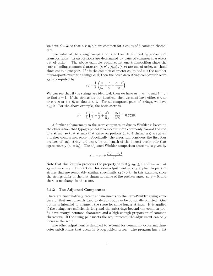
A further enhancement to the score computation due to Winkler is based onthe observation that typographical errors occur more commonly toward the endof a string, so that strings that agree on prefixes (1 to 4 characters) are givena higher comparison score. Specifically, the algorithm considers the first fourprefixes of each string and lets p be the length of the longest prefix pair thatagree exactly (ai = bi). The adjusted Winkler comparison score sW is given by

sW = sJ +p (1− sJ)

10.

Note that this formula preserves the property that 0 ≤ sW ≤ 1 and sW = 1⇔sJ = 1⇔ α = β. In practice, this score adjustment is only applied to pairs ofstrings that are reasonably similar, specifically sJ > 0.7. In this example, sincethe strings differ in the first character, none of the prefixes agree, so p = 0, andthere is no change in the score.

3.1.2 The Adjusted Comparator

There are two relatively recent enhancements to the Jaro-Winkler string com-parator that are currently used by default, but can be optionally omitted. Oneoption is intended to augment the score for some longer strings. It is appliedif the strings are sufficiently long and the substrings beyond the common pre-fix have enough common characters and a high enough proportion of commoncharacters. If the string pair meets the requirements, the adjustment can onlyincrease the score.The other adjustment is designed to account for commonly occurring char-

acter subtitutions that occur in typographical error. The program has a list

4

of pairs of similar characters, which represent common typographical substitu-tions, based on common spelling mistakes, visual similarity, or keyboard prox-imity. The current version uses 36 such pairs. After the common charactershave been matched, the program looks through the unmatched characters to seeif an unmatched character in one string is similar to an unmatched character inthe other string, allowing character in the other string to be similar to at mostone character from the first string. If s is the total number of similar characterpairs counted, then the adjusted count cs of common characters is given by

cs = c+ 0.3s

and if this adjustment is in force then the basic Jaro score sJ is actually com-puted by

sJ =1

3

µcsm+

csn+

c− t

c

¶.

In our example, the only unmatched character in the first string is b, and theonly characters similar to b in the list of similar characters are v and 8, whichdo not occur in the second string, so no similar character adjustment is made.

3.2 Edit Distance String Comparator

Another approach to string comparison is based on edit (or Levinshtein) dis-tance. These measures are determined by the minimum number of edit stepsrequired to convert one string to the other. We will call edit distance themethod that uses insertion, deletion, or substitution for possible edit steps. An-other possibility is to restrict the edit steps to just insertion or deletion. Theminimum number of edit steps can be computed using a straightforward dy-namic programming algorithm with complexity O

¡n2¢, where n is the length

of the strings. The idea of the dynamic programming algorithm is to computethe shortest distance for all prefix pairs, where we compute the cost of the cur-rent prefix pair from the minimum of the previous minimal prefix costs plus thecost of the edit step that converts the earlier prefix to the current one. Sincethe strings representing Census names are fairly short (generally less than 20characters), the algorithm executes very quickly. These distance measures havethe property that they are metrics. It is clear that the distance functions arereflexive and symmetric, and the triangle inequality can be verified by inductionon the length of the strings. In our studies, we have used edit distance sincethis seems to capture an appropriate edit process. Many misspellings involvesubstituting one letter for another.In order to use one of these distance functions as a string comparator and

to compare its performance to the Jaro-Winkler string comparator, we see from(1) that it is helpful to convert the distance value to a number between 0 and 1,with 1 representing complete agreement. The resulting function may be called asimilarity function [Navarro]. We do this by considering the maximum numberof edit steps possible to convert one string to another. For edit distance, if thestrings of length m and n with m ≤ n have no characters in common, then the

5

minimum edit sequence is to do m substitutions followed by n−m insertions ordeletions, for a total of n edit steps. Thus we can scale edit distance into our[0, 1] comparison measure by letting the comparison value x be given by

x = 1− d

n

where d is the edit distance between the two strings and n is their maximumlength.When first experimenting with this edit similarity function, we found that it

could be too severe, penalizing a string pair for every difference without givingsufficient credit for common features. For example, the pair {Stan, Stanley}has an adjusted Jaro-Winkler score of 0.9142 while this edit distance similarityfunction evaluates the pair at 0.5714. We decided to modify the edit distancesimilarity score by taking into consideration the length of the longest commonsubsequence (lcs) of the two strings. This length can be computed similarly asthe edit distance by counting the number of identity steps (no edit required)in the shortest edit sequence. However, this is only necessarily true when theavailable edit steps are restricted to insertion and deletion [Wagner]. This canbe done with a separate but parallel distance computation. Since the maximumpossible length of an lcs is m, the length of the shorter string, we can get an lcssimilarity score y from

y =l

m

where l is the length of an lcs. We derive a modified edit distance similarityscore sedt taking the average of these two scores

sedt =x+ y

2.

We note that the modified edit distance score for {Stan,Stanley} is 0.7857.

3.3 Adaptive String Comparator

The edit distance metric counts the minimum number of character edits requiredto convert one string to another, each edit having a unit cost. We consider theproblem of having the edit cost function, instead of being constant, depend onthe characters involved. If we are trying to decide whether two strings bothrepresent the same word, then edit changes that represent common misspellingsor typographical errors could cost less than rare changes, so that the scoremight better reflect the plausibility that the two strings are equivalent. Sourcesof typographical error could be written misspelling, phonetic misspelling, keystroke errors, or scanning errors. Since different data sets might be subjectto different proportions of these error sources, it might be helpful if the editcost function could adapt to the data sets at hand. We describe a method forassigning these costs and define an adaptive string comparator based on the editcomparator model.

6

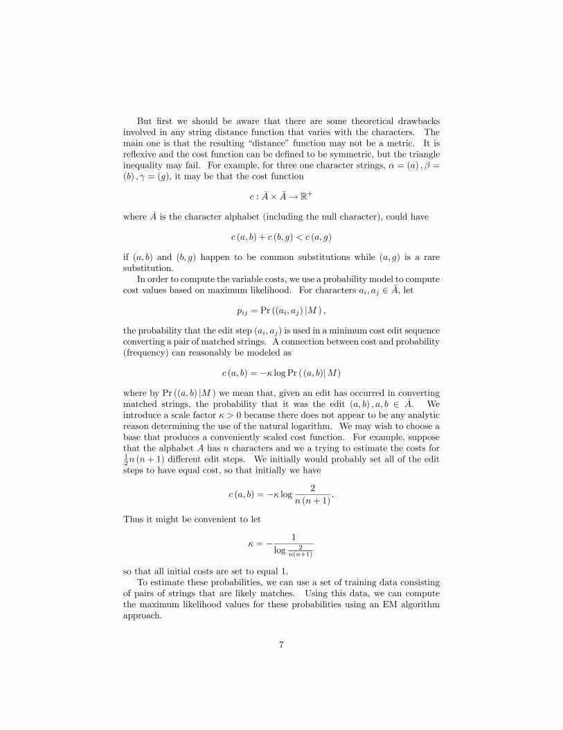
But first we should be aware that there are some theoretical drawbacksinvolved in any string distance function that varies with the characters. Themain one is that the resulting “distance” function may not be a metric. It isreflexive and the cost function can be defined to be symmetric, but the triangleinequality may fail. For example, for three one character strings, α = (a) , β =(b) , γ = (g), it may be that the cost function

c : A× A→ R+

where A is the character alphabet (including the null character), could have

c (a, b) + c (b, g) < c (a, g)

if (a, b) and (b, g) happen to be common substitutions while (a, g) is a raresubstitution.In order to compute the variable costs, we use a probability model to compute

cost values based on maximum likelihood. For characters ai, aj ∈ A, let

pij = Pr ((ai, aj) |M ) ,

the probability that the edit step (ai, aj) is used in a minimum cost edit sequenceconverting a pair of matched strings. A connection between cost and probability(frequency) can reasonably be modeled as

c (a, b) = −κ log Pr ((a, b)|M)

where by Pr ((a, b) |M ) we mean that, given an edit has occurred in convertingmatched strings, the probability that it was the edit (a, b) , a, b ∈ A. Weintroduce a scale factor κ > 0 because there does not appear to be any analyticreason determining the use of the natural logarithm. We may wish to choose abase that produces a conveniently scaled cost function. For example, supposethat the alphabet A has n characters and we a trying to estimate the costs for12n (n+ 1) different edit steps. We initially would probably set all of the editsteps to have equal cost, so that initially we have

c (a, b) = −κ log 2

n (n+ 1).

Thus it might be convenient to let

κ = − 1

log 2n(n+1)

so that all initial costs are set to equal 1.To estimate these probabilities, we can use a set of training data consisting

of pairs of strings that are likely matches. Using this data, we can computethe maximum likelihood values for these probabilities using an EM algorithmapproach.

7

3.3.1 Maximum Likelihood

For each edit step (ai, bj) ∈ S ⊂ C∗ × C∗, we want to maximize

L =Yi,j

Pr ((ai, bj)|M)nij

where the data nij is the count of times the edit step was used and the param-eters are Pr ((ai, bj)|M), which is the probability of using the edit step (ai, bj)in a minimum cost edit of a pair of strings which both represent the same word.For a given count of the edit steps, the maximum likelihood occurs for

Pr ((ai, bj)|M) = nijN

(2)

where N is the total of all edit steps used. That is, we count the edit stepsused in the least cost edit path for all pairs of likely matching strings. Ristad[Ristad] also uses a probabilistic approach, but counts all edit step through allpossible paths. Using the least cost path seemed to be the more reasonablemodel for this application.Using the EM algorithm to maximize likelihood, we can initialize the param-

eter values with equal probabilities; for the E-step, we can count the numbernij of each edit steps used; for the M-step, we use the edit frequencies to revisethe edit probability parameters according to (2).

3.3.2 Developing a Similarity Score

While the above calculation is simple and converges quickly, the resulting costsmay lack some rationality. For example, for a given pair of characters (a, b),we may get a cost function c where

c (a, b) > c (a, ε) + c (ε, b)

that is, the cost of substitution can exceed cost of the equivalent insertion anddeletion. We modify the cost function by replacing the substitution cost by theminimum of these two. For a given pair of strings, we can then use the dynamicprogramming algorithm to compute their adaptive edit “distance”. To convertthis to a comparison score, we still need to divide by the maximum distance.The concept of maximum distance between two unrelated strings is less clear.Instead of simply counting the maximum number of edit steps, we have to decideon what costs to assign to each step. By analogy to the edit step count, wecompute a maximum distance ma by

ma =mXk=1

c0 (ak, bk) +nX

k=m+1

c (bk, )

where

c0 (a, b) =½

c (a, b) if a 6= b1 if a = b

8

If ca is the total minimum adaptive edit cost, we compute an adaptive similarityscore sadp by

sadp =1

2

µcama

+l

m

¶where l is the lcs length as before.

3.3.3 The Training Data Set

In order to calculate our maximum likelihood costs, we need a set of trainingdata. To produce a training data set, we run the matching software on the testfiles and get a printout of matched record pairs sorted by match score. As withstandard matching procedure, we examine the list and choose a cutoff scoreabove which all the pairs are designated matches. We then read in the pairsof designated matched records and write out the pairs of first or last nameswhere neither name is blank and the names are not identical strings. Thisforms the initial training data set of pairs of names that come from matchedrecords but have some spelling discrepancy. We want pairs of strings that likelyboth represent the same name. This file is edited further to eliminate the mostunlikely agreeing pairs. We read in these name pairs and compute the standardJaro-Winkler string comparator score. We then sort the pairs by this scoreand eliminate low scoring pairs that do not appear to be different spellingsof the same name. The result is a set that represents pairs of strings thatare matched but which have spelling errors. This procedure could be used toproduce training data from any pair of files designated for record linkage.

4 Testing the String ComparatorsOur test data consists of the three 1990 Census/PES file pairs that have beenclerically reviewed. So far we have used the largest set (STL) to explore themethodology for our comparison tests. In the future we can apply the samemethods to the other two sets to see if the results are consistent. We use theCensus Bureau matcher software to produce our training data and test data.The standard blocking strategy for these sets has been to use the cluster numberand the first character of the last name. We used this to produce the first namedata, but it presumably introduces a bias for the last name data, so we reran thesoftware blocking on cluster number and first character of first name to producethe last name data.Specifically, for each of these two runs, we ran the counting program and

used the output of the EM algorithm to obtain parameter estimates for theagreement probabilities. Then we used these parameter estimates to run thematching program. As described above, we used the output of the matcherto produce training data sets. For the test data, we considered every recordpair brought together by the blocking criterion. When blocking on last namecharacter, we printed out every pair of first names from these record pairs.Since we had clerically reviewed truth data, we printed these first name pairs

9

to two different files, depending on whether the pair came from a match pair ora non-match pair. We did the analogous thing for last names under the otherblocking criterion.

4.1 Linear Regression

Although we have scaled all of the string comparator functions to produce scoresbetween 0 and 1, these scores are not modeled as probabilities. The specificscores have no particular significance. It does not make much sense to comparethe scores of two string comparators directly. However, increasing comparatorscores are supposed to indicate increasing confidence of string pair matching.Thus valid string comparators should exhibit a common trend. Thus we com-pare two comparators by computing a linear regression of the scores of one ontothe other.We computed separate regressions for first name pairs and last name pairs.

In both cases, we used the set of pairs that came from the designated matchrecords. We reduced the sets by eliminating all identical string pairs and allrepetitions of the same string pairs to arrive at a set of unique, unequal stringpairs. We then computed residuals for both the sets from match pairs and fromnon-match pairs.

4.1.1 The Jaro-Winkler String Comparators

We compared the results of the Jaro-Winkler string comparators, with andwithout the two adjustments for long strings and similar characters. We didthis partially to try to perceive the effects of the adjustments and partially toget a baseline for similar string comparators.Not surprisingly, the two J-W versions are highly correlated (0.99) and the

linear regressions are a tight fit, the last name pairs slightly better than the firstname pairs (first R2 = 0.98, last R2 = 0.99). The first name pairs have veryfew residuals greater than 0.1, the last name pairs have none (first 99.8%, last100.0% have |r| < 0.1).

4.1.2 Edit Distance and Adaptive String Comparators

When we compare the edit distance and adaptive string comparators, the resultsare very similar. The are similarly correlated (0.99) and the regression fit isabout as good (first R2 = 0.97, last 0.99). There are only slightly more residualslarger than 0.1 (first 99.4%, last 98.8% have |r| < 0.1).

4.1.3 The Jaro-Winkler and Edit Distance String Comparators

We compared the adjusted Jaro-Winkler string comparator to both the editdistance string comparator and the adaptive string comparator. Although thesestill show strong similarities, they are not as similar as the previous comparisons.The J-W and edit distance comparators are strongly correlated (first 0.93, last0.95) and have good regression fits (first R2 = 0.86, last R2 = 0.90). The

10

number of larger residuals is greater (first 91.9%, last 90.0% have |r| < 0.1).The J-W and adaptive string comparators are almost as correlated (first 0.92,last 0.94) and slightly less good regression fits (first R2 = 0.85, last R2 = 0.89)with slightly fewer large residual pairs (first 92.8%, last 90.5% have |r| < 0.1).

4.2 Comparison Weight Function

We have so far compared the string comparator functions by regressing one oftheir scores on the other, observing how much one set of scores explains theother, and examining cases where the actual and predicted score most differ.We note that for pairs where the scores were low, a larger residual probably didnot matter for the record linkage application. This is because in the recordlinkage application, we use the comparator scores to evaluate a comparisonweight function

w (x) = logPr (γ = x |M )

Pr (γ = x |U )to assign a comparison weight. To evaluate the performance of a string com-parator for the record linkage application, we need to compare the results ofthe comparison weight function. In order to do this, we need an appropriatecomparison weight function for each comparator.As we see from its definition, the evaluation of the comparison weight func-

tion depends on probabilities that are conditioned on the true match status ofthe records. While this may not be known in general, we take advantage ofour Census test decks with reviewed match status to approximate a reasonablecomparison weight function for each comparator. For first and last names,we use the full sets of pairs from matches and pairs from non-matches, not re-moving duplicates or exact matches. We calculate the string comparator valuefor each pair and count the number of pairs whose values fall within each cellof a partition of [0, 1]. To summarize the results, we see by inspection thatgenerally the cell values of w (x) decrease as x decreases from 1, until x gets toa point c where the values of w (x) tend to level out. This corresponds to ournotion that string comparator scores below a certain level should indicate totaldisagreement. In the region [c, 1] where w (x) seems to be increasing, we fit astraight line. The final approximated comparison weight function is a straightline truncated below by the total disagreement weight and truncated above bythe total agreement weight.For this data set, we found that for all four comparators, the first names

resulted in a better fit than the last names. The worst fitting cases suggestthat a logistic curve might be a better fit. The regression lines for all of theJ-W cases were similar and those of the edit and adaptive methods were allsimilar. The J-W slopes were greater than the edit or adaptive slopes. This isconsistent with the score regressions, where edit or adaptive scores the predictedby the J-W scores are always larger than the original edit or adaptive scores on[0, 1].

11

4.3 Matching Weight Comparison

We compare the performance of the string comparators by comparing the agree-ment weights assigned to string pairs, using the estimated comparison weightfunction for each comparator. We looked at the four sets of first and last name,match and non-match records separately. Again our sets are reduced to theunique, non-identical pairs. We compute the weight differences between pairsof comparators, the same pairs for which we computed regression lines.Again, as we might anticipate from the regression results, on the whole, the

differences are not great. To give a snapshot example, suppose we consider asubstantial weight difference to be 1.75. For the first and last name agreementand disagreement weights, this represents roughly 25% of the length of the totalweight interval. The following is a table shows the percentage of pairs in ourdata sets for which [∆] < 1.75, where ∆ is the difference between the two weightassignments.

First Mat First Non Last Mat Last NonBasic & Adjusted J-W 99.1 99.8 99.9 99.8Edit & Adaptive 100.0 99.9 99.8 99.9J-W & Edit 96.1 97.8 98.0 99.2J-W & Adaptive 96.4 98.0 97.8 99.3

(3)Table (3) indicates that the string comparators assign agreement weights thatare fairly similar for the preponderance of the sample data pairs. The non-matches have a lot of agreement since most of the pairs have very little similarityand thus get assigned the full disagreement weight.The weight difference distributions suggest very modest differences between

the basic and adjusted J-W comparators, which is not too surprising since theyare highly similar. If anything, the differences between the edit and adaptivecomparators are even less. This calls into question the benefit of all of the extrawork involved in calibrating and computing the variable edit weights. Althoughthe results are similar, the edit and adaptive string comparators show somewhatgreater differences with the adjusted J-W comparator. This reflects that theyhave different structures.On the one hand this is reassuring that reasonably valid string comparators

should all provide fairly consistent results to the record linkage algorithm. Onthe other hand, it does not help us to choose between them. The differentcomparators might significantly affect the record linkage results for the caseswith the most extreme differences, so we considered these individual cases.Subjectively there does not appear to be a strong case for favoring the results

of any of these comparators over the others. In general when one looks at theextreme cases for a matched pair set, the comparator assigning the higher weightappears to be doing a better job. When one looks at the extreme cases fromthe non-match pairs, the comparator assigning the higher weight appears to bedoing worse.

12

For example, when we look at the differences between the basic and adjustedJ-W comparators, as the Table (3) suggests, there are not many cases of largechanges. The changes that improve the matching are countered by similarchanges that do not improve the matching. Likewise, comparing the edit andadaptive comparators, there are even fewer large changes. Among these, thecomparator giving the better weight assignment is fairly evenly balanced. Inthese direct comparisons, there does not appear to be a case for using thecharacter specific adjustments.When we compare the adjusted J-W comparator to either the edit or adap-

tive comparator, we do see more sizable differences. These differences point outthe distinct properties of the two types of string comparator, but they do notclearly establish which comparator is doing the better record linkage job. Thebasic difference is that the J-W string comparator is good for identifying pairsof strings with permuted common characters, while the edit-based comparatorsare good for finding pairs of strings with significant common substrings.To cite some specific examples, there are cases where the J-W compara-

tor assigns the full disagreement weight and the edit and adaptive weight aremore than 5 points higher, resulting in a strong agreement weight. The J-Wcomparator is exacting on short strings, so that pairs such as {UZ, U Z} and{JK, JIK} that receive full disagreement weight from J-W almost or more than6 points higher weights from the edit and adaptive comparators respectively.Likewise, the substring property gives similarly strong weight increases to {Ivy,Ivory}, {Sara, Asara}, {Tony, Anthony}, {Dale, Lyndale}, and {Leroy, Roy},which are subjectively credible as positive agreement weight pairs. On theother hand, these comparators give similar weight increases to {Amy, Tammy},{Randy, Ray}, and {Tracy, Ray}, which appear to be less likely matched names.Likewise among last names, the edit and adaptive comparators give a weightincrease of from 3 to 5 points to double names like {Shell Gladney, Gladney} or{Cohee-Wheeler, Wheeler}. On the other hand, there are also strong increasesfor {Edwards, Ward}, {Hermann, Mann}, and {Ore, Moore}.The differences where the J-W weight exceeds the edit or adaptive weight

are not as large as the largest of the above differences. On the positive side, theJ-W exceeds the others by around 3 points for {Tolando, Talonda}, {Bilenda,Belinda}, and Louanda, Lavonda}, but also less convincingly for {Geraldine,Regna}, {Cornelius, Rocile}, and {Lenora, Veronica}. Actually there aresmaller differences for the last name match pairs, and the largest differencelast name non-match pairs appear to be awarding slightly positive agreementweight to unlikely agreement pairs. By just looking at the largest weight differ-ences for last name pairs, the edit and adaptive comparators appear to performa little better than the adjusted J-W comparator.By just subjectively evaluating the comparators’ performance on some ex-

amples, we can get an idea about how they perform differently, but it does notprovide convincing evidence for evaluating their relative performance for therecord linkage application. Of course, the relevant test for that would be tocompare the effects of the different comparators on the linkage of the recordpairs. Since many other factors are involved in the record linkage, it would be

13

difficult to isolate particular comparator effects. Since it is difficult to observedefinitive evidence of superiority by examining the comparator results directly,it would be even harder to discern when masked by many other contributions.

5 SummaryWe have length of the longest common substring along with edit distance to de-fine a string similarity function to compare with the Jaro-Winkler string com-parator. We create an adaptive variation on the edit distance cost functionto adjust edit costs based on frequency of use. We compare the results ofthe different comparators on first and last name pairs from Census files. Re-gression analysis shows that they all have strong common linear trends. Bydeveloping a record linkage weight assignment function for each comparator, wecan examine differences in weight assignments between the comparators. Inboth the Jaro-Winkler case and the edit/adaptive case, we do not detect anyreal advantage from using either adjustment for commonly used substitutions.While largely very similar, the Jaro-Winkler comparator does have some largeweight differences with the edit or adaptive comparators. There is some slightindication that the edit approach is doing more good than harm, but this wouldhave to be confirmed using other data sets.

References[Navarro] Navarro, G. “A Guided Tour to Approximate String Matching.”

ACM Computing Surveys. Vol. 33, No. 1, March 2001, pp. 31—88.

[Ristad] Ristad, E. S. and Yianilos, P. N. “Learning String Edit Distance.”IEEE Transactions on Pattern Analysis and Machine Intelligence.1998, 20(5):522—532.

[Wagner] Wagner, R. and Fisher, M. “The String to String Correction Prob-lem.” Journal of the Association for Computing Machinery. Vol. 21,No. 1, January 1974, pp.168—173.

[Winkler] Winkler, W. E. The State of Record Linkage and Cur-rent Research Problems. Statistics of Income Division, In-ternal Revenue Service Publication R99/04. Available fromhttp://www.census.gov/srd/www/byname.html.

A Appendix

A.1 Linear Regression

We provide a sample of the linear regression graphs of the scores from one stringcomparator onto the scores of another. In Fig (1) we see a strong linear relation

14

Figure 1: Basic and Adjusted Jaro-Winkler Scores

between the Jaro-Winkler scores with and without the adjustments for similarcharacters and longer strings.

In Fig (2), the edit scores with and without adjusted costs also show a stronglinear relation. Several of the more outlying points have scores low enough thatthey likely both receive full disagreement weight.

In Fig (3), the adjusted Jaro-Winkler and adaptive edit scores show a domi-nant linear relationship, but there are more outliers and some of these representscores high enough to result in some significant weight differences.

A.2 Comparison Weight Function

In Fig (4) we have plotted the binned comparison weights adjusted Jaro-Winklerscores for first names. The weights appear to line up well for scores above 0.6.In Fig (5) we plot the regression line for these points.In Fig (6) we plot the last name comparison weights for edit distance. The

weights for scores above 0.4 are not as linearly aligned, but the linear regressionin Fig (7) provides a fair approximation.

A.3 Matching Weight Comparison

As we have seen in Table (3), using the computed weight comparison functions,the different string comparators assign weights of small differences to the bulkof name pairs. To give a little idea of where the comparators differ the most,we give some tables representing the largest differences.

15

Figure 2: Edit and Adaptive Scores

Figure 3: Adjusted Jaro-Winkler Score and Adaptive Edit Score

16

Figure 4: Adjusted Jaro-Winkler Comparison Weights

17

Figure 5: Adjusted Jaro-Winkler Weight Regression Line

Figure 6: Edit Distance Comparison Weights

18

Figure 7: Edit Distance Weight Regression Line

A.3.1 The Jaro-Winkler String Comparators

In Table (4) we are looking at the last name pairs coming from matching recordswhere the adjusted J-W weight most exceeds the basic J-W weight. Even thelargest differences produced by the adjustments are not too dramatic and it isnot clear that all of the pairs should have their comparison weight increased.

Adjusted Weight > Basic WeightLast Name Match Pairs J-W Scores J-W Weights

Name 1 Name 2 Basic Adj Basic Adj DiffGRICE GRIFFIN 0.6762 0.7973 −2.8908 −0.6981 2.1927GORDON JORDAN 0.7778 0.8778 −0.6127 1.1317 1.7444HAMER HAYMOND 0.6762 0.7684 −2.8908 −1.3566 1.534JONES JAMES 0.7600 0.8488 −1.0114 0.4726 1.4839THOMPSON JOHNSON 0.7131 0.8011 −2.0632 −0.6127 1.4504CURRUTHERS CORORRETHRS 0.7832 0.8697 −0.4915 0.9474 1.4389

(4)In Table (5) we see the last name pairs coming from non-matching records

where the adjusted J-W weight most exceeds the basic J-W weight. Here thelargest differences arise from raising basic weights at or near full disagreementweight to adjusted weights that are still negative but nearer zero. Again it is

19

not clear that these adjustments would be helpful for the matching.

Adjusted Weight > Basic WeightLast Name Non-Match Pairs J-W Scores J-W WeightsName 1 Name 2 Basic Adj Basic Adj Diff

MASEK MASCARE 0.6762 0.8213 −2.8908 −0.1522 2.7386GARANZINI GARAVAGLIA 0.6852 0.8238 −2.6891 −0.0966 2.5925THURMAN THOMPSON 0.6905 0.8167 −2.5704 −0.2583 2.3121MCCULLOUGH MCCASKILL 0.6852 0.8092 −2.6891 −0.4285 2.2606SCHMIDT SCHUH 0.6762 0.7973 −2.8908 −0.6981 2.1927COLEMAN KOMADINA 0.6905 0.8113 −2.5704 −0.3810 2.1894GRIFFIN GREEN 0.6762 0.7958 −2.8908 −0.7327 2.1580JACKSON JAMES 0.6762 0.7958 −2.8908 −0.7327 2.1580

(5)Since the J-W adjustments can only raise the basic score, the basic weight

exceeds the adjusted weight most in cases where the adjustments had no effectand the scores remained the same. Tables (6) and (7) list the largest weightdifferences for match pairs and non-match pairs respectively. There a severalother pairs with weight differences of size about 0.5. These differences shouldhave small effect on the record linkage.

Basic Weight > Adjusted WeightLast Name Match Pairs J-W Scores J-W WeightsName 1 Name 2 Basic Adj Basic Adj DiffSTUBBS STUDES 0.8444 0.8444 0.8823 0.3735 −0.5088BOYD BOLDY 0.8267 0.8267 0.4836 −0.0309 −0.5145DOWD DOWELL 0.8250 0.8250 0.4462 −0.0688 −0.5150VAUHNS VAUGHER 0.8222 0.8222 0.3839 −0.1320 −0.5159COAD JACOAD 0.8056 0.8056 0.0102 −0.5110 −0.5213TIMM TZMMS 0.8050 0.8050 −0.0023 −0.5237 −0.5214BUNCH BUNTIT 0.7900 0.7900 −0.3386 −0.8649 −0.5263HEE YEE 0.7778 0.7778 −0.6127 −1.1429 −0.5302

(6)

20

Basic Weight > Adjusted WeightLast Name Non-Match Pairs J-W Scores J-W WeightsName 1 Name 2 Basic Adj Basic Adj Diff

ALT BALL 0.7222 0.7222 −1.8585 −2.4065 −0.5480ORE COLE 0.7222 0.7222 −1.8585 −2.4065 −0.5480WARD EDWARD 0.7222 0.7222 −1.8585 −2.4065 −0.5480KEY HUEY 0.7222 0.7222 −1.8585 −2.4065 −0.5480OGE LOVE 0.7222 0.7222 −1.8585 −2.4065 −0.5480RICHARDSON CARR 0.7167 0.7167 −1.9831 −2.5329 −0.5498BILL WILLIAMS 0.7083 0.7083 −2.1700 −2.7225 −0.5525HALL CHANDLER 0.7083 0.7083 −2.1700 −2.7225 −0.5525MCDOWELL COLE 0.7083 0.7083 −2.1700 −2.7225 −0.5525HULL FULLAURD 0.7083 0.7083 −2.1700 −2.7225 −0.5525WILLIAMS HILL 0.7083 0.7083 −2.1700 −2.7225 −0.5525KERR MAYBERRY 0.7083 0.7083 −2.1700 −2.7225 −0.5525

(7)

A.3.2 Adaptive and Edit Weight

The differences between edit weight and adaptive weight are generally smallerbut more symmetric than between the two forms of J-W weight. For the lastname pairs where the adaptive weight most exceeds the edit weight, we see thatfor the match pairs in Table (8) and non-match pairs in Table (9), the largestadaptive weight differences do not generally appear to benefit record linkage.

Adaptive Weight > Edit WeightLast Name Match Pairs Scores WeightsName 1 Name 2 Adapt Edit Adapt Edit DiffPOLK POKE 0.8600 0.7000 2.3178 0.3345 1.9833YABER YORBRO 0.6175 0.4667 −1.4263 −2.9108 1.4845GANES GAINS 0.8539 0.7333 2.2246 0.8332 1.3914JONES JOHNSON 0.7690 0.6476 0.9129 −0.4490 1.3619YATES YAT 0.8943 0.8000 2.8487 1.8304 1.0183

(8)Adaptive Weight > Edit Weight

Last Name Non-Match Pairs Scores WeightsName 1 Name 2 Adapt Edit Adapt Edit DiffBAKER BLACK 0.7083 0.5000 −0.0242 −2.6572 2.6330HARRIS SHEARER 0.7598 0.5714 0.7716 −1.5887 2.3603OWENS BROWN 0.6735 0.4667 −0.5616 −2.9108 2.3492BLASE SIEBELS 0.6725 0.4381 −0.5763 −2.9108 2.3345YATES BRYANT 0.6699 0.4833 −0.6161 −2.9065 2.2904PHILLIPS HEMPHILL 0.7261 0.5417 0.2508 −2.0339 2.2847AWLS WELLS 0.7557 0.5750 0.7084 −1.5353 2.2437

(9)In Tables (10) and (11) we have examples of last name pairs where the edit

21

weight most exceeds the adaptive weight. Again in the match pair and non-match pair cases, the differences are fairly small and do not appear to indicategenerally better weight assignment for matching.

Edit Weight > Adaptive WeightLast Name Match Pairs Scores WeightsName 1 Name 2 Adp Edit Adp Edit DiffBLEIN KLEIN 0.7616 0.8000 0.7993 1.8304 −1.0311HAYES BANES 0.5586 0.6000 −2.3359 −1.1613 −1.1746WEST WEBB 0.5570 0.6000 −2.3605 −1.1613 −1.1992HEE YEE 0.5819 0.6667 −1.9755 −0.1641 −1.8114

(10)Edit Weight > Adaptive Weight

Last Name Non-Match Pairs Scores WeightsName 1 Name 2 Adp Edit Adp Edit DiffPEPPERS SELLERS 0.5058 0.5714 −2.9108 −1.5887 −1.3221MAIER LABER 0.5482 0.6000 −2.4963 −1.1613 −1.3350REEDER KREIGER 0.6122 0.6667 −1.5082 −0.1641 −1.3441JORDAN MORGAN 0.6095 0.6667 −1.5493 −0.1641 −1.3852WILSON DIXSON 0.6078 0.6667 −1.5764 −0.1641 −1.4123REEDER KRIEGER 0.5999 0.6667 −1.6983 −0.1641 −1.5342WARNER PARKER 0.5965 0.6667 −1.7498 −0.1641 −1.5857TINKER BINGER 0.5943 0.6667 −1.7836 −0.1641 −1.6195TEIBER BERNER 0.5283 0.6071 −2.8028 −1.0545 −1.7483BOND BOXX 0.4822 0.6000 −2.9108 −1.1613 −1.7495PALMER WALKER 0.5824 0.6667 −1.9678 −0.1641 −1.8037

(11)

A.3.3 J-W and Edit Weight

There are larger differences between either edit or adaptive weight and basicor adjusted Jaro-Winkler weight than are found between either pair of similarcomparators. In Table (12) we see the largest weight differences for last namesfrom matched pairs. Here we see one of the properties of edit score is that itgives credit for large common substrings even when they do not occur in thesame parts of each string. For last names, this picks up some cases of double lastnames where the other string just has the second part of the name. Instead oftotal disagreement weight, they get assigned a small positive agreement weight.Incidentally, for the first name pairs, the largest weight differences involved shortstrings, especially initials. When comparing, for example, “L C” and “LC",the J-W comparator results in a low disagreement weight while the edit andadaptive comparators produce a high agreement weight.

22

Edit Weight > J-W WeightLast Name Match Pairs Scores Weights Diff

Name 1 Name 2 Edit J-W Edit J-WCOHEE-WHEELER WHEELER 0.7692 0.6264 1.3701 −2.9108 4.2809SHELL GLADNEY GLADNEY 0.7692 0.3352 1.3701 −2.9108 4.2809STRUB-TURNAGE TURNAGE 0.7692 0.4860 1.3701 −2.9108 4.2809JONES-ATKINS ATKINS 0.7500 0.5500 1.0825 −2.9108 3.9933FOSTER-ARNITZ ARNITZ 0.7308 0.4021 0.7948 −2.9108 3.7056JONES GOSBY GOSBY 0.7273 0.5855 0.7425 −2.9108 3.6533JONES PARKER JONES 0.7083 0.4561 0.4592 −2.9108 3.3700SKAGGE SLOAN SLOAN 0.7083 0.5506 0.4592 −2.9108 3.3700COAD JACOAD 0.8333 0.8056 2.3290 −0.5110 2.8401

(12)In Table (13) we see the last name non-match pairs for which the edit weight

most exceeds the J-W weight. While these pairs may not be matches, the editcomparator is registering a recognizable similarity between the strings.

Edit Weight > J-W WeightLast Name Non-Match Pairs Scores WeightsName 1 Name 2 Edit J-W Edit J-W Diff

ORE MOORE 0.8000 0.5644 1.8304 −2.9108 4.7412WARD EDWARD 0.8333 0.7222 2.3290 −2.4065 4.7356EDWARDS WARD 0.7857 0.6905 1.6167 −2.9108 4.5275HERMANN MANN 0.7857 0.5821 1.6167 −2.9108 4.5275WOODARD WARD 0.7857 0.6345 1.6167 −2.9108 4.5275WARD STEWARD 0.7857 0.0000 1.6167 −2.9108 4.5275BAUER WOLFBAUER 0.7778 0.0000 1.4980 −2.9108 4.4088BELL CAMPBELL 0.7500 0.4958 1.0825 −2.9108 3.9933WARD POWLLARD 0.7500 0.5333 1.0825 −2.9108 3.9933MAY MCNALLY 0.7143 0.6508 0.5482 −2.9108 3.4590

(13)In Table (14) we see the last name match pairs where the J-W weight most

exceeds the edit weight. The differences here are not as large as in Table(12),and although these pair come from match records, only about half of them looklike likely matching strings, so that the justification for the higher weight is notobvious..

23

J-W Weight > Edit WeightLast Name Match Pairs Scores Weights

Name 1 Name 2 Edit J-W Edit J-W DiffJONES JOHNSON 0.6476 0.8738 −0.4490 1.0419 −1.4909THOMPSON JOHNSON 0.5357 0.8011 −2.1230 −0.6127 −1.5102HAINES HAYMES 0.6667 0.8880 −0.1641 1.3642 −1.5283DOLIE DOYLE 0.7333 0.9347 0.8332 2.4257 −1.5925GANES GAINS 0.7333 0.9347 0.8332 2.4257 −1.5925JONES JAMES 0.6000 0.8488 −1.1613 0.4726 −1.6339WRATHY WORTHY 0.7500 0.9475 1.0825 2.7176 −1.6351CURRUTHERS CORORRETHRS 0.6227 0.8697 −0.8214 0.9474 −1.7688COVINGTON COUTION 0.5794 0.8463 −1.4700 0.4168 −1.8868CHEATHER CHEETMA 0.5893 0.8932 −1.3216 1.4821 −2.8037

(14)In Table (15) we have the largest differences with the J-W weight exceeding

the edit weight for non-match last name pairs. Here most of the differencesare larger than in Table (14), generally raising a near total disagreement editweight to a near zero to slightly positive J-W weight. The name pairs generallylook convincingly unmatched.

J-W Weight > Edit WeightLast Name Non-Match Pairs Scores WeightsName 1 Name 2 Edit J-W Edit J-W Diff

ADAMS KAMADULSKI 0.4833 0.8216 −2.9065 −0.1468 −2.7597CARNAGHI CUNNINGHAM 0.4500 0.8252 −2.9108 −0.0644 −2.8464OWENS JONES 0.5000 0.8375 −2.6572 0.2155 −2.8727LEWIS WILLIS 0.4667 0.8274 −2.9108 −0.0153 −2.8955WILSON LEWIS 0.3833 0.8274 −2.9108 −0.0153 −2.8955HOLLINS ALLISON 0.4464 0.8286 −2.9108 0.0124 −2.9232STEWART ATWATER 0.4464 0.8286 −2.9108 0.0124 −2.9232THOMPSON MCPHERSON 0.4792 0.8332 −2.9108 0.1174 −3.0282BEANS BASKIN 0.4167 0.8347 −2.9108 0.1525 −3.0633WALKER FOWLER 0.5000 0.8516 −2.6572 0.5360 −3.1932FOWLER WALTER 0.5000 0.8516 −2.6572 0.5360 −3.1932STOKER KUSTER 0.5000 0.8516 −2.6572 0.5360 −3.1932SPINKS PERKINS 0.4762 0.8405 −2.9108 0.2844 −3.1952HAMILTON HOLMAN 0.4375 0.8458 −2.9108 0.4044 −3.3152NICHOLSON JOHNSON 0.5079 0.8636 −2.5385 0.8088 −3.3472

(15)

24