wiiw Working Paper 148 · Based on a newly constructed multi-country input-output table including...
52
MAY 2018
Transcript of wiiw Working Paper 148 · Based on a newly constructed multi-country input-output table including...
MAY 2018


Based on a newly constructed multi-country input-output table including all European countries, we
structural gravity framework. The results point towards strong positive effects on trade for the SAA
countries, but only small effects for the EU Member States. Conducting a counterfactual analysis, the
paper gives an indication of the magnitude of the positive impacts on GDP for these countries. In
addition, a detailed industry breakdown of these effects is provided.
- -

ff
Table 1: Summary of SAA process.............................................................................................................8
Table 2: Estimation results .......................................................................................................................11
Table 3: Estimation results .......................................................................................................................11
Table 4: Total exports, by industry group .................................................................................................13
Table 5: Value added exports, by industry group .....................................................................................14
Table 6: Total exports, by detailed manufacturing industry ......................................................................15
.........................................................................17
Table 8: Full equilibrium changes, Western Balkan EU enlargement.......................................................18
Figure 1: Export growth of Westbalkan countries with the EU28, by type of export .................................10
Figure 2: ....................................................................17
Figure 3: Change in real GDP in case of Western Balkan EU accession.................................................19
Appendix
.......................................................................26
Table A.2: Country coverage of Supply and Use Tables ..........................................................................27
Table C.3: Estimation results ....................................................................................................................33
Table C.4: Estimation results ....................................................................................................................34
Table C.5: Estimation results ....................................................................................................................34
Table C.6: Estimation results ....................................................................................................................35
Table C.7: Estimation results ....................................................................................................................36
Table C.8: Estimation results ....................................................................................................................37

1 Introduction
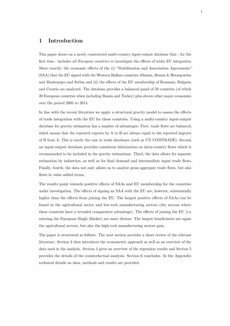
This paper draws on a newly constructed multi-country input-output database that - for the
first time - includes all European countries to investigate the effects of wider EU integration.
More exactly, the economic effects of the (i) “Stabilisation and Association Agreements”
(SAA) that the EU signed with the Western Balkan countries Albania, Bosnia & Herzegowina
and Montenegro and Serbia and (ii) the effects of the EU membership of Romania, Bulgaria
and Croatia are analysed. The database provides a balanced panel of 50 countries (of which
39 European countries when including Russia and Turkey) plus eleven other major economies
over the period 2005 to 2014.
In line with the recent literature we apply a structural gravity model to assess the effects
of trade integration with the EU for these countries. Using a multi-country input-output
database for gravity estimation has a number of advantages: First, trade flows are balanced,
which means that the reported exports by A to B are always equal to the reported imports
of B from A. This is rarely the case in trade databases (such as UN COMTRADE). Second,
an input-output database provides consistent information on intra-country flows which is
recommended to be included in the gravity estimations. Third, the data allows for separate
estimation by industries, as well as for final demand and intermediate input trade flows.
Finally, fourth, the data not only allows us to analyse gross aggregate trade flows, but also
flows in value added terms.
The results point towards positive effects of SAAs and EU membership for the countries
under investigation. The effects of signing an SAA with the EU are, however, substantially
higher than the effects from joining the EU. The largest positive effects of SAAs can be
found in the agricultural sector and low-tech manufacturing sectors (the sectors where
these countries have a revealed comparative advantage). The effects of joining the EU (i.e.
entering the European Single Market) are more diverse: The largest beneficiaries are again
the agricultural sectors, but also the high-tech manufacturing sectors gain.
The paper is structured as follows: The next section provides a short review of the relevant
literature. Section 3 then introduces the econometric approach as well as an overview of the
data used in the analysis. Section 4 gives an overview of the regression results and Section 5
provides the details of the counterfactual analysis. Section 6 concludes. In the Appendix
technical details on data, methods and results are provided.
1
2 Literature Review
2.1 Gravity Model
Methodologically, the paper follows the recent strand of literature which started with
Anderson and Van Wincoop (2003). They introduced the concept of “multilateral resistances”
which solved the econometric problem that trade between two nations depends not only on
the distance (or trade friction) between the two nations, but also on the distances to other
nations. Furthermore, they popularised the idea that these multilateral resistances can be
estimated using exporter-time and importer-time fixed effects.
Silva and Tenreyro (2006) showed that the gravity estimates are biased when using ordinary
least squares and suggested estimating the equation with Poisson pseudo-maximum likelihood
(PPML) instead. Recently, Fally (2015) argued that estimating a gravity specification with
exporter-time and importer-time fixed effects using PPML has the additional advantage
of being immediately consistent with the multilateral resistances from theory and the
equilibrium constraints they entail.
Baier and Bergstrand (2007) stressed the importance of controlling for the endogeneity of
FTAs. Their recommendation to use country-pair fixed effects is now standard practice in
the empirical implementation. P. H. Egger and Nigai (2015) reiterate this point by arguing
that trade costs are best accounted for by asymmetric pair fixed effects. They demonstrate
that – using simulations – pair fixed effects lead to substantially less biased coefficients
compared to empirical specifications which use a parameterised function for trade costs
(such as bilateral distance, common language, etc).
Larch, Wanner, Yotov, and Zylkin (2017) re-asses the effect of a currency union (not to be
confused with custom union, which is also sometimes abbreviated with ”CU”) using data on
trade flows from more than 200 countries over 65 years. They rely on a “full set” of fixed
effects, i.e., exporter-time, importer-time and pair fixed effects. Using the recommended
PPML estimator for this exercise, they find that currency unions, in general, have a large
positive and significant effect, except the European Monetary Union (EMU). The effect of
the EMU is small, though positive, however insignificant (when using the recommended
clustered standard errors). Though they analyse the effects of the EMU, their result is
indicative for our case looking at the effects of a European customs union as done in this
paper.
Finally, Anderson, Larch, and Yotov (2015) show how the structural gravity framework
can be employed for counterfactual analysis, using iterations of constraint regressions. In
2
section 5 we follow their recommendations when we estimate scenarios of EU accession for
the Western Balkan countries.
So, the recommendations about how to estimate the gravity equation are quite clear: use
exporter-time and importer-time fixed effects to account for the multilateral resistances and
use (asymmetric) pair fixed effects to take care of the bilateral trade costs. Trade policy
variables are bilateral and time-varying and can be additionally included in the estimation.
The findings and best practices of this research area were summarised comprehensively in
the “Advanced Guide to Trade Policy Analysis: The Structural Gravity Model” by Yotov,
Piermartini, Monteiro, and Larch (2016).
2.2 Stabilisation and Association Agreements
This paper particularly considers the potential economic effects of the EU “Stabilisation and
Association Agreements” (SAA). These are signed by countries that are candidates to join
the European Union (EU). Before signing such a SAA, the “Stabilisation and Agreement
Process” needs to be passed. This process aims at initiating reforms that contribute to
stability and the democratic development and will eventually lead to EU membership.
The literature on the economic effects of the SAA is rather scarce and most of the contribu-
tions focus on particular countries. For example, Zahariadis (2007) using the GTAP model
estimates that the Stabilisation and Assocation Process could bring an increase in GDP of
as much as 1.5% in Albania. He proposes that even 2% could be possible, if Albania would
fully implement all EU legislation on trade related standards and modernise all custom
administration.
Pula (2014) provides an overview concerning the impacts on various countries and draws
conclusions for Kosovo. Monastiriotis, Kallioras, and Petrakos (2014) study the impact
of pre-accession agreements in Central and Eastern European countries and argue that
such agreements accelerate growth, though highly unevenly across regions. Based on these
results they derive similar conclusions on the new European Neighbourhood Policy (ENP)
framework.
Sebastian (2008) is more cautious and raises questions if the current Western Balkan
candidate countries are able to fulfill the required reforms and if the EU’s policies were
adequate. She concludes that the “lack of clear benchmarks, the EU’s divisions, and the
uncertainty around the SAP” may “have diminished the effectiveness of EU inducements”.
This paper contributes to this literature providing evidence from a cross-country perspective
3
based on the newly created multi-country input-output database and applying a structural
gravity modelling approach.
3 Estimation strategy and data
3.1 Gravity equation approach
To assess impacts of SAA and EU accession we apply a gravity model to bilateral international
trade flows which allows us to capture the effects of various trade policy measures on these
flows. These equations can be derived from several different angles, from supply side or from
demand side oriented models as neatly summarised in Head (2014) or Yotov et al. (2016).
These contributions provide an overview over the possible theoretical underpinnings of the
gravity equation as well as practical guidelines for estimation and trade policy analysis.
Specifically, we employ a “standard” formulation1 of the gravity equation:
Xij,t = exp[πi,t + χj,t + µij + β1FTAij,t + β2SAAij,t
+ β3EFTAij,t + β4CUij,t + βτ τ̃ij,t
]× εij (1)
where i and j are the exporter and importer indices and t is a time index. The dependent
variable Xij,t denotes either gross exports or value-added exports between the exporter and
the importer.
Country-pair fixed effects are denoted by µij . We also include a set of exporter-time and
importer-time fixed effects given by πi,t and χj,t. For capturing trade policy effects two
sets of variables are included: First, τ̃ij,t denotes bilateral tariffs. Second, the four variables
FTAij,t, SAAij,t, EFTAij,t and CUij,t capture whether a free trade agreement (FTA), a
“Stabilisation and Assocation Agreement” (SAA), a free trade agreement with a EFTA
member (EFTA) or a customs union (CU) exists between the two countries i and j at time
t.
Equation (1) is the recommended specification by Yotov et al. (2016) as the country-time
fixed effects control for any unobservable multilateral resistances. Additionally, the pair fixed
effects take care of potential endogenous trade policy as stressed by Baier and Bergstrand
(2007).1For the interested reader we provide results for another formulation of the gravity model, one using
economic mass variables instead of fixed effects, in part C in the appendix.
4
This gravity equation is estimated at the national but also industry level as well as for final
demand and intermediate trade flows. Estimating equation (1) at the industry level (or for
demand components) is, due to the so-called “separability” property of structural gravity
models, analogous to estimating the equation at the country level.
3.2 Data
3.2.1 Country sample and time period
The data on gross exports and value added exports are based on multi-country input-output
tables (MC-IOTs) that include all European countries (except Kosovo and Belarus) together
with a couple of other major economies in the world. We refer to this database as the “wiiw
Wider Europe Multi-Country Input-Output Database”. It contains 50 countries and 32
industries and comprises the period 2005-2014.
This database resulted from an effort to provide data for a larger set of countries as so
far available in the World-Input-Output Database (WIOD); see Timmer, Dietzenbacher,
Los, Stehrer, and Vries (2015) and the recent WIOD release 2016 documented in Timmer,
Los, Stehrer, and de Vries (2016). In particular this effort aimed at including all European
countries to be able to capture production linkages between all European countries. At this
stage all EU-28 countries together with the non-EU European countries Iceland, Norway,
Switzerland, the five Western Balkan countries (Albania, Bosnia & Herzegovina, Former
Yugoslav Republic of Macedonia (Macedonia hereafter), Montenegro and Serbia), Russia,
Turkey and Ukraine are included.2 Additionally, the data covers the biggest non-European
economies, such as Australia, Brazil, Canada, China, India, Indonesia, Japan, Mexico, South
Korea, Taiwan, the United States of America. The Input-Output database furthermore
includes a Rest-of-the-World region, which however is not used in the gravity estimations.
These MC-IOTs have been constructed similarly to the approach used for the World Input-
Output Database as documented in Timmer et al. (2015) and the recent update which has
been undertaken Timmer et al. (2016). For most European countries a full set of supply
and use tables has been available for at least one year according to ESA2010 (SNA2008)
methodology. Particularly, most countries now also provide use tables in basic prices
as well as import use tables. Concerning the EU-28 countries, import use tables were
however missing for Germany, Latvia and Luxembourg while for Greece, Netherlands and
Spain no valuation matrices have been available (i.e. the use tables are only provided in2Unfortunately, Kosovo and Belarus are still missing from a full coverage of all European countries due
to severe data constraints.
5
purchaser’s prices) and therefore also no import use matrices are reported. In these cases
import use tables have been constructed according to WIOD methodology. Concerning
the European non-EU Member States decent data have been available for Norway and
Switzerland. Iceland’s supply and use tables are benchmarked on Norway’s tables. For
the Western Balkan countries data for Albania and Macedonia could be collected; however,
import use tables have not been available. For Bosnia & Herzegovina and Serbia the tables
from Macedonia have been used as a benchmark. Similarly, we use the Croatian supply
and use tables for Montenegro and the Polish tables for Ukraine as a benchmark. Supply
and use tables for the remaining non-European countries have been taken from the WIOD
release 2016.
To arrive at a proper time series the supply and use tables have been benchmarked to
official National Accounts data which have generally been available for all countries (though
some slight adjustments had to be made in some cases at the industry level). However,
data availability forced us to aggregate to 32 industries, as more detailed data on services
industries have been missing for a number of European non-EU countries. There are further
some distinct differences between the construction process of our database and that of the
WIOD (release 2016) which are reported in detail in the Appendix A).3 The most important
difference is that we use import use tables in the construction process to the extent available
which has implications for the size of re-exports and the size of gross export flows reported
in the MC-IOTs. In particular, the levels of re-exports have been calculated based on the
information provided in the export column of the import use tables.4
A second difference exists concerning the calculation of domestic transport margins on
exports which in this case have been assumed to be zero.5
Third, bilateral trade flows might differ because the RAS-procedure which has to be applied
to balance trade flows and reconcile them with values from the global supply and use tables
start from a different set of benchmark values. Finally, the construction of the rest-of-world
category has been undertaken in a different manner. In particular, the strategy was that we
calculate a consistent supply and use system for the rest-of-world. Only after this step, the3It should be noted that in this effort the construction process for all European countries differ from
the WIOD approach though the same method has been applied for all countries. For the non-Europeancountries WIOD Release 2016 data have been taken.
4In the WIOD Release 2016 re-exports have been calculated as the difference between imports and totaluse in case the total use is smaller than imports. The figures provided in the import use tables howevershow that re-exports take a much larger amount. As re-exports vanish from the system in the way theinternational use tables are calculated the level of gross trade flows tends to be lower. It should however benoted that this does not impact on the share of value added exports in GDP or the domestic and foreigncontent of exports.
5In In the WIOD Release 2016 part of the domestic transport margins have been allocated to exportstherefore reducing the level of exports.
6
global supply and use tables are transformed to an global input-output tables by assuming
an fixed product sales structure (called “Model D”).6
3.2.2 Inter- and intranational trade flows
In the estimation, we use two types of dependent variables: First, as usually done, bilateral
gross trade flows are investigated. Secondly, the MC-IOTs allow us to take bilateral value
added exports as a dependent variable. These are computed according to Johnson and
Noguera (2012); see Stehrer (2012) for an explanation of the calculation of value-added
exports. This allows us to investigate if bilateral value added trade flows behave differently
compared to the gross trade flows.
Yotov et al. (2016) argue that the inclusion of intra-national trade flows is a very important
condition to arrive at unbiased gravity estimates. Fortunately, these can be extracted
from the the intra- and international trade flows of both the gross exports and the value-
added exports on sectoral level from the “wiiw Wider Europe Multi-Country Input-Output
database”. The intra-national value added flow is simply the total produced value added
minus the sum of all value added exports.
3.2.3 Trade agreements
Data capturing free trade agreements and custom unions are taken from Mario Larch’s
database of regional trade agreements (see P. Egger and Larch (2008)). Because we already
include bilateral fixed effects, bilateral trade agreements that are in effect over the whole time
period (in our case 2005 to 2014) are deleted from the database to avoid collinearity. For
example, the effect of the custom union between Austria and Germany is already subsumed
in the bilateral dummy of Austria and Germany.
There are in total five countries in our sample that initiated trade agreements between 2005
and 2014. The first four countries are Albania, Bosnia & Herzegowina and Montenegro and
Serbia. They signed “Stabilisation and Association Agreements” (SAA) with the members
of the European Union and – more or less at the same time – free trade agreements with the
EFTA states7. Table 18 gives an overview of the dates of these agreements for the countries
of our interest.6In the WIOD release Model D is applied to all countries in the database; then in a second step the
IOT of the rest-of-world is calibrated. See Eurostat (2008) for a detailed explanation of the “Model D” thetransformation of supply and use tables to a symmetric input-output table.
7Iceland, Norway and Switzerland. Liechtenstein is also a member of EFTA, but not in our countrysample.
8“IA” stands for “Interim Agreement”.
7
An SAA is usually implemented by a potential EU accession candidate in which it commits to
certain political and economical reforms. We separate SAA and EFTA free trade agreements
in our analysis into an SAA and an EFTA dummy as they may have different effects.
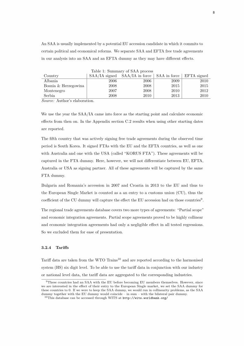
Table 1: Summary of SAA processCountry SAA/IA signed SAA/IA in force SAA in force EFTA signedAlbania 2006 2006 2009 2010Bosnia & Herzegowina 2008 2008 2015 2015Montenegro 2007 2008 2010 2012Serbia 2008 2010 2013 2010
Source: Author’s elaboration.
We use the year the SAA/IA came into force as the starting point and calculate economic
effects from then on. In the Appendix section C.2 results when using other starting dates
are reported.
The fifth country that was actively signing free trade agreements during the observed time
period is South Korea. It signed FTAs with the EU and the EFTA countries, as well as one
with Australia and one with the USA (called “KORUS FTA”). These agreements will be
captured in the FTA dummy. Here, however, we will not differentiate between EU, EFTA,
Australia or USA as signing partner. All of these agreements will be captured by the same
FTA dummy.
Bulgaria and Romania’s accession in 2007 and Croatia in 2013 to the EU and thus to
the European Single Market is counted as a an entry to a customs union (CU), thus the
coefficient of the CU dummy will capture the effect the EU accession had on those countries9.
The regional trade agreements database covers two more types of agreements: “Partial scope”
and economic integration agreements. Partial scope agreements proved to be highly collinear
and economic integration agreements had only a negligible effect in all tested regressions.
So we excluded them for ease of presentation.
3.2.4 Tariffs
Tariff data are taken from the WTO Trains10 and are reported according to the harmonised
system (HS) six digit level. To be able to use the tariff data in conjunction with our industry
or national level data, the tariff data are aggregated to the corresponding industries.9These countries had an SAA with the EU before becoming EU members themselves. However, since
we are interested in the effect of their entry to the European Single market, we set the SAA dummy forthese countries to 0. If we were to keep the SAA dummy, we would run in collinearity problems, as the SAAdummy together with the EU dummy would coincide – in sum – with the bilateral pair dummy.
10This database can be accessed through WITS at http://wits.worldbank.org/
8
It is, however, not fully clear what the best way of aggregation is: One could simply use
the arithmetic mean of tariffs over all HS codes. This may lead to misleading and arbitrary
results, since all products have the same weight in this procedure, irrespective of their
importance in the bilateral trade flow. The second option, aggregation by weighted means,
has a similar caveat: Since tariffs influence the trade flows quantitatively, products with
high tariffs will have lower trade volumes and thus also lower weights11. Bouët, Decreux,
Fontagné, Jean, and Laborde (2004) recommend to use a “reference group weighted method”
to aggregate tariffs: This method assigns a given importer country X to a reference group
and uses then the exports of the trade partner country Y to the reference group of X as
weights in the aggregation. See Bouët et al. (2004) for a more thorough treatment of the
issue.
We observe, however, no big (systematic) differences in the aggregated tariffs. All three
types of aggregated tariffs follow the same path over time and are already very low at the
beginning of our observed period. Thus it comes as no surprise that the results in the gravity
estimation do not differ much between the three types of tariffs. For this reason and for
easier interpretation we only report results with the weighted tariffs12.
11It is revealing to think of two extreme cases: One, where there is a tariff so high that it completelyinhibits trade (and there is no trade of that product). Secondly, a situation where there is no tariff at allbut the traded quantity is huge. In both cases, the contribution of that product to the aggregated tariff willbe 0.
12Results with the mean tariff and reference group weighted tariffs are given in the Appendix in sectionC.1.
9
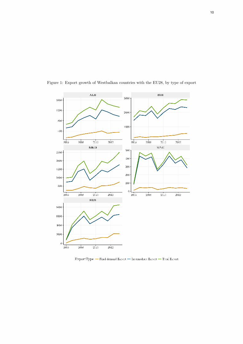
Figure 1: Export growth of Westbalkan countries with the EU28, by type of export
10
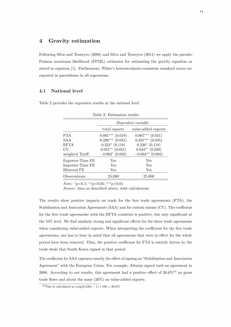
4 Gravity estimation
Following Silva and Tenreyro (2006) and Silva and Tenreyro (2011) we apply the pseudo-
Poisson maximum likelihood (PPML) estimator for estimating the gravity equation as
stated in equation (1). Furthermore, White’s heteroscedastic-consistent standard errors are
reported in parentheses in all regressions.
4.1 National level
Table 2 provides the regression results at the national level.
Table 2: Estimation results
Dependent variable:total exports value-added exports
FTA 0.091∗∗∗ (0.019) 0.067∗∗∗ (0.021)SAA 0.236∗∗∗ (0.031) 0.231∗∗∗ (0.035)EFTA 0.224∗ (0.118) 0.226∗ (0.118)CU 0.051∗∗ (0.021) 0.044∗∗ (0.020)weighted Tariff −0.003∗ (0.002) −0.004∗∗ (0.002)Exporter-Time FE Yes YesImporter-Time FE Yes YesBilateral FE Yes YesObservations 25,000 25,000
Note: ∗p<0.1; ∗∗p<0.05; ∗∗∗p<0.01Source: data as described above, wiiw calculations
The results show positive impacts on trade for the free trade agreements (FTA), the
Stabilisation and Assocation Agreements (SAA) and for custom unions (CU). The coefficient
for the free trade agreements with the EFTA countries is positive, but only significant at
the 10% level. We find similarly strong and significant effects for the three trade agreements
when considering value-added exports. When interpreting the coefficient for the free trade
agreements, one has to bear in mind that all agreements that were in effect for the whole
period have been removed. Thus, the positive coefficient for FTA is entirely driven by the
trade deals that South Korea signed in that period.
The coefficient for SAA captures exactly the effect of signing an “Stabilisation and Association
Agreement” with the European Union. For example, Albania signed such an agreement in
2006. According to our results, this agreement had a positive effect of 26.6%13 on gross
trade flows and about the same (26%) on value-added exports.13This is calculated as (exp(0.236) − 1) ∗ 100 = 26.6%
11
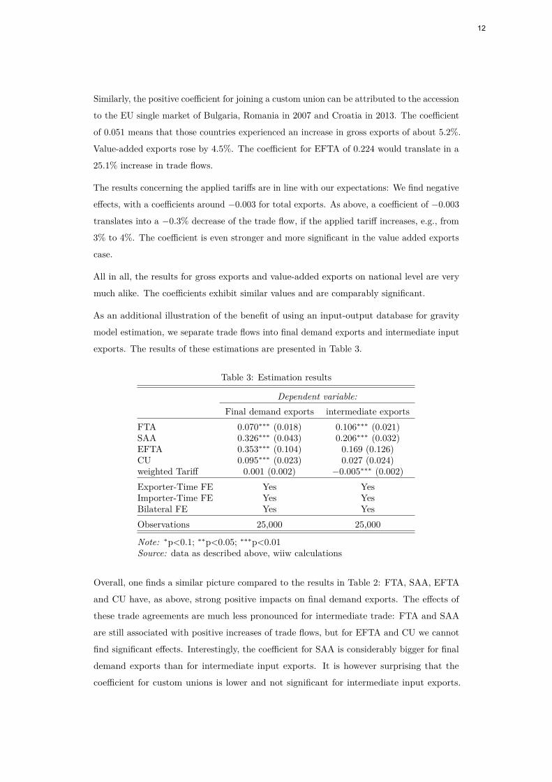
Similarly, the positive coefficient for joining a custom union can be attributed to the accession
to the EU single market of Bulgaria, Romania in 2007 and Croatia in 2013. The coefficient
of 0.051 means that those countries experienced an increase in gross exports of about 5.2%.
Value-added exports rose by 4.5%. The coefficient for EFTA of 0.224 would translate in a
25.1% increase in trade flows.
The results concerning the applied tariffs are in line with our expectations: We find negative
effects, with a coefficients around −0.003 for total exports. As above, a coefficient of −0.003
translates into a −0.3% decrease of the trade flow, if the applied tariff increases, e.g., from
3% to 4%. The coefficient is even stronger and more significant in the value added exports
case.
All in all, the results for gross exports and value-added exports on national level are very
much alike. The coefficients exhibit similar values and are comparably significant.
As an additional illustration of the benefit of using an input-output database for gravity
model estimation, we separate trade flows into final demand exports and intermediate input
exports. The results of these estimations are presented in Table 3.
Table 3: Estimation results
Dependent variable:Final demand exports intermediate exports
FTA 0.070∗∗∗ (0.018) 0.106∗∗∗ (0.021)SAA 0.326∗∗∗ (0.043) 0.206∗∗∗ (0.032)EFTA 0.353∗∗∗ (0.104) 0.169 (0.126)CU 0.095∗∗∗ (0.023) 0.027 (0.024)weighted Tariff 0.001 (0.002) −0.005∗∗∗ (0.002)Exporter-Time FE Yes YesImporter-Time FE Yes YesBilateral FE Yes YesObservations 25,000 25,000
Note: ∗p<0.1; ∗∗p<0.05; ∗∗∗p<0.01Source: data as described above, wiiw calculations
Overall, one finds a similar picture compared to the results in Table 2: FTA, SAA, EFTA
and CU have, as above, strong positive impacts on final demand exports. The effects of
these trade agreements are much less pronounced for intermediate trade: FTA and SAA
are still associated with positive increases of trade flows, but for EFTA and CU we cannot
find significant effects. Interestingly, the coefficient for SAA is considerably bigger for final
demand exports than for intermediate input exports. It is however surprising that the
coefficient for custom unions is lower and not significant for intermediate input exports.
12
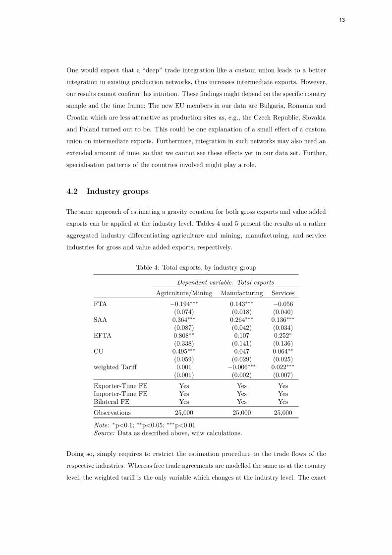
One would expect that a “deep” trade integration like a custom union leads to a better
integration in existing production networks, thus increases intermediate exports. However,
our results cannot confirm this intuition. These findings might depend on the specific country
sample and the time frame: The new EU members in our data are Bulgaria, Romania and
Croatia which are less attractive as production sites as, e.g., the Czech Republic, Slovakia
and Poland turned out to be. This could be one explanation of a small effect of a custom
union on intermediate exports. Furthermore, integration in such networks may also need an
extended amount of time, so that we cannot see these effects yet in our data set. Further,
specialisation patterns of the countries involved might play a role.
4.2 Industry groups
The same approach of estimating a gravity equation for both gross exports and value added
exports can be applied at the industry level. Tables 4 and 5 present the results at a rather
aggregated industry differentiating agriculture and mining, manufacturing, and service
industries for gross and value added exports, respectively.
Table 4: Total exports, by industry group
Dependent variable: Total exportsAgriculture/Mining Manufacturing Services
FTA −0.194∗∗∗ 0.143∗∗∗ −0.056(0.074) (0.018) (0.040)
SAA 0.364∗∗∗ 0.264∗∗∗ 0.136∗∗∗
(0.087) (0.042) (0.034)EFTA 0.808∗∗ 0.107 0.252∗
(0.338) (0.141) (0.136)CU 0.495∗∗∗ 0.047 0.064∗∗
(0.059) (0.029) (0.025)weighted Tariff 0.001 −0.006∗∗∗ 0.022∗∗∗
(0.001) (0.002) (0.007)Exporter-Time FE Yes Yes YesImporter-Time FE Yes Yes YesBilateral FE Yes Yes YesObservations 25,000 25,000 25,000
Note: ∗p<0.1; ∗∗p<0.05; ∗∗∗p<0.01Source: Data as described above, wiiw calculations.
Doing so, simply requires to restrict the estimation procedure to the trade flows of the
respective industries. Whereas free trade agreements are modelled the same as at the country
level, the weighted tariff is the only variable which changes at the industry level. The exact
13
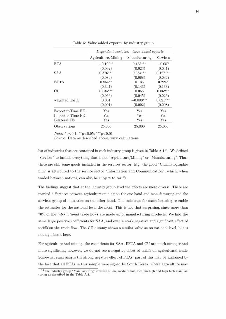
Table 5: Value added exports, by industry group
Dependent variable: Value added exportsAgriculture/Mining Manufacturing Services
FTA −0.192∗∗ 0.138∗∗∗ −0.057(0.092) (0.023) (0.041)
SAA 0.376∗∗∗ 0.364∗∗∗ 0.127∗∗∗
(0.089) (0.068) (0.034)EFTA 0.864∗∗ 0.135 0.224∗
(0.347) (0.143) (0.133)CU 0.535∗∗∗ 0.056 0.062∗∗
(0.066) (0.045) (0.026)weighted Tariff 0.001 −0.008∗∗∗ 0.021∗∗∗
(0.001) (0.002) (0.008)Exporter-Time FE Yes Yes YesImporter-Time FE Yes Yes YesBilateral FE Yes Yes YesObservations 25,000 25,000 25,000
Note: ∗p<0.1; ∗∗p<0.05; ∗∗∗p<0.01Source: Data as described above, wiiw calculations.
list of industries that are contained in each industry group is given in Table A.114. We defined
“Services” to include everything that is not “Agriculture/Mining” or “Manufacturing”. Thus,
there are still some goods included in the services sector. E.g. the good “Cinematographic
film” is attributed to the service sector “Information and Communication”, which, when
traded between nations, can also be subject to tariffs.
The findings suggest that at the industry group level the effects are more diverse: There are
marked differences between agriculture/mining on the one hand and manufacturing and the
services group of industries on the other hand. The estimates for manufacturing resemble
the estimates for the national level the most. This is not that surprising, since more than
70% of the international trade flows are made up of manufacturing products. We find the
same large positive coefficients for SAA, and even a stark negative and significant effect of
tariffs on the trade flow. The CU dummy shows a similar value as on national level, but is
not significant here.
For agriculture and mining, the coefficients for SAA, EFTA and CU are much stronger and
more significant, however, we do not see a negative effect of tariffs on agricultural trade.
Somewhat surprising is the strong negative effect of FTAs: part of this may be explained by
the fact that all FTAs in this sample were signed by South Korea, where agriculture may14The industry group “Manufacturing” consists of low, medium-low, medium-high and high tech manufac-
turing as described in the Table A.1.
14
not feature that prominently.
We find a negative (though insignificant) impact of FTA for services, but also positive signs
for SAAs and custom unions. The coefficient for tariffs is positive and significant.
Services play a minor (but growing) role only in international trade, with about 19% of total
exports being services. These are, however, a major part (67%) of intranational trade flows.
This circumstance, along with the fact that trade in services is a more complex phenomenon
(e.g. the modes of services trade play an important role) and its statistical recording is still
developing allows only for cautious interpretations of the estimation results for service trade.
As at the national level, the results for gross exports and value added exports resemble each
other very much. When comparing Tables 4 and 5 we see that the coefficients are again
very similar. The coefficients for value added exports are in general slightly larger, implying
that they seem to react more to all sorts of regional trade agreements and tariffs than gross
exports.
Finally, we disaggregate the manufacturing industries even further into low, medium-low,
medium-high and high tech manufacturing industries. Again, the free trade agreements
are the same as at the national level, but the trade flows and the tariffs are at the specific
industry level. Since the results for value added and gross exports are again similar, we only
report results for gross exports.
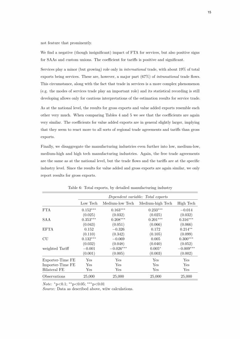
Table 6: Total exports, by detailed manufacturing industry
Dependent variable: Total exportsLow Tech Medium-low Tech Medium-high Tech High Tech
FTA 0.152∗∗∗ 0.163∗∗∗ 0.233∗∗∗ −0.014(0.025) (0.032) (0.025) (0.032)
SAA 0.353∗∗∗ 0.208∗∗∗ 0.201∗∗∗ 0.316∗∗∗
(0.043) (0.051) (0.066) (0.066)EFTA 0.152 −0.326 0.172 0.214∗∗
(0.110) (0.342) (0.105) (0.099)CU 0.132∗∗∗ −0.069 0.005 0.300∗∗∗
(0.032) (0.048) (0.040) (0.052)weighted Tariff −0.001 −0.026∗∗∗ 0.005∗ −0.009∗∗∗
(0.001) (0.005) (0.003) (0.002)Exporter-Time FE Yes Yes Yes YesImporter-Time FE Yes Yes Yes YesBilateral FE Yes Yes Yes YesObservations 25,000 25,000 25,000 25,000
Note: ∗p<0.1; ∗∗p<0.05; ∗∗∗p<0.01Source: Data as described above, wiiw calculations.
15
We see from the results in Table 6 that the benefits of trade agreements are not evenly
distributed among the manufacturing industries. Gains from SAAs are found in all man-
ufacturing subgroups, but low and high tech industries tend to gain more than the two
“medium”-tech industries. The coefficient for custom unions is positive and significant in the
low and high tech sector, but not in the medium tech sectors. We even find a negative effect
in the medium-low sector, however not significant. The EFTA dummy is only significant in
the high tech sector.
Tariffs have a negative and highly significant impact in the medium-low tech and the high
tech sector, as well as a positive effect in the medium-high sector which is significant at the
10% level.
5 Counterfactual exercises
In this section we provide estimates of the effects of signing an SAA or joining the EU on
GDP using a general equilibrium setting. A short overview over the estimation process is
given in Appendix B, but interested readers are referred to the comprehensive explanations
given in Yotov et al. (2016) or Anderson et al. (2015).
In the first part we investigate the effects of signing an SAA with Serbia in 2010. In the
second part we investigate the economic effects of a potential EU enlargement of the Western
Balkan countries in this framework.
5.1 Effect of SAA on Serbia
First, we use our results from Table 2 to answer the question “By how much did Serbia’s
economy grow, due to the enforcement of the SAA in 2010?”. We have already seen that the
SAAs substantially increased trade flows. But it will be also interesting to see what impact
the SAA had on GDP in Serbia and other countries.
To carry out this counterfactual scenario, we set the SAA dummy for Serbia and the EU
countries to 0. Then, we follow the steps as described in Appendix B. The results will then
tell us what the GDP of Serbia would have been (and thus how much it profited), had they
not signed the SAA in 2010.
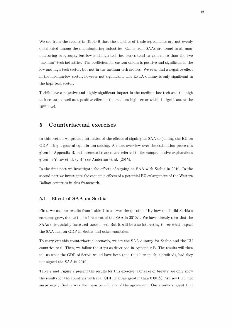
Table 7 and Figure 2 present the results for this exercise. For sake of brevity, we only show
the results for the countries with real GDP changes greater than 0.001%. We see that, not
surprisingly, Serbia was the main beneficiary of the agreement: Our results suggest that
16
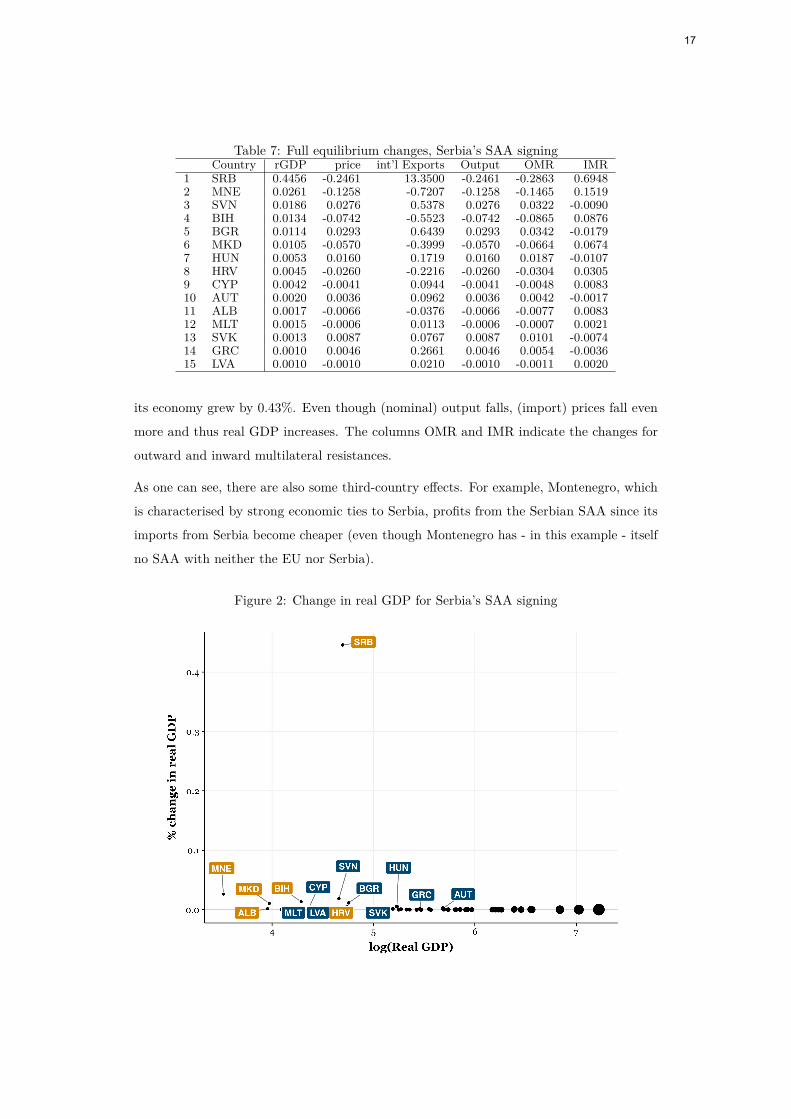
Table 7: Full equilibrium changes, Serbia’s SAA signingCountry rGDP price int’l Exports Output OMR IMR
1 SRB 0.4456 -0.2461 13.3500 -0.2461 -0.2863 0.69482 MNE 0.0261 -0.1258 -0.7207 -0.1258 -0.1465 0.15193 SVN 0.0186 0.0276 0.5378 0.0276 0.0322 -0.00904 BIH 0.0134 -0.0742 -0.5523 -0.0742 -0.0865 0.08765 BGR 0.0114 0.0293 0.6439 0.0293 0.0342 -0.01796 MKD 0.0105 -0.0570 -0.3999 -0.0570 -0.0664 0.06747 HUN 0.0053 0.0160 0.1719 0.0160 0.0187 -0.01078 HRV 0.0045 -0.0260 -0.2216 -0.0260 -0.0304 0.03059 CYP 0.0042 -0.0041 0.0944 -0.0041 -0.0048 0.008310 AUT 0.0020 0.0036 0.0962 0.0036 0.0042 -0.001711 ALB 0.0017 -0.0066 -0.0376 -0.0066 -0.0077 0.008312 MLT 0.0015 -0.0006 0.0113 -0.0006 -0.0007 0.002113 SVK 0.0013 0.0087 0.0767 0.0087 0.0101 -0.007414 GRC 0.0010 0.0046 0.2661 0.0046 0.0054 -0.003615 LVA 0.0010 -0.0010 0.0210 -0.0010 -0.0011 0.0020
its economy grew by 0.43%. Even though (nominal) output falls, (import) prices fall even
more and thus real GDP increases. The columns OMR and IMR indicate the changes for
outward and inward multilateral resistances.
As one can see, there are also some third-country effects. For example, Montenegro, which
is characterised by strong economic ties to Serbia, profits from the Serbian SAA since its
imports from Serbia become cheaper (even though Montenegro has - in this example - itself
no SAA with neither the EU nor Serbia).
Figure 2: Change in real GDP for Serbia’s SAA signing
17
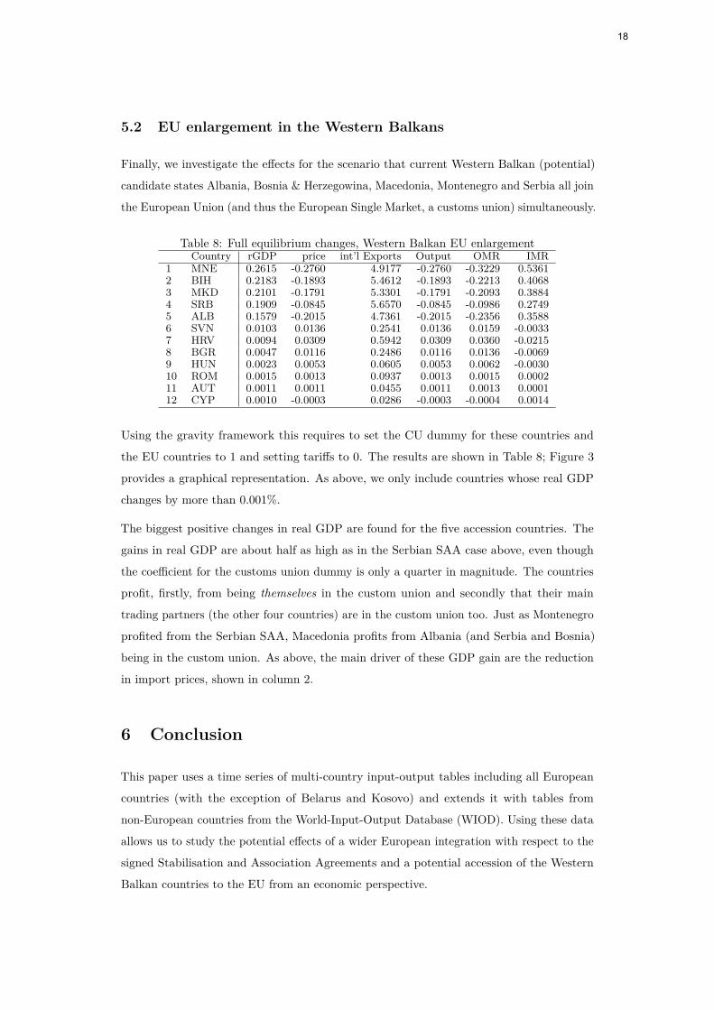
5.2 EU enlargement in the Western Balkans
Finally, we investigate the effects for the scenario that current Western Balkan (potential)
candidate states Albania, Bosnia & Herzegowina, Macedonia, Montenegro and Serbia all join
the European Union (and thus the European Single Market, a customs union) simultaneously.
Table 8: Full equilibrium changes, Western Balkan EU enlargementCountry rGDP price int’l Exports Output OMR IMR
1 MNE 0.2615 -0.2760 4.9177 -0.2760 -0.3229 0.53612 BIH 0.2183 -0.1893 5.4612 -0.1893 -0.2213 0.40683 MKD 0.2101 -0.1791 5.3301 -0.1791 -0.2093 0.38844 SRB 0.1909 -0.0845 5.6570 -0.0845 -0.0986 0.27495 ALB 0.1579 -0.2015 4.7361 -0.2015 -0.2356 0.35886 SVN 0.0103 0.0136 0.2541 0.0136 0.0159 -0.00337 HRV 0.0094 0.0309 0.5942 0.0309 0.0360 -0.02158 BGR 0.0047 0.0116 0.2486 0.0116 0.0136 -0.00699 HUN 0.0023 0.0053 0.0605 0.0053 0.0062 -0.003010 ROM 0.0015 0.0013 0.0937 0.0013 0.0015 0.000211 AUT 0.0011 0.0011 0.0455 0.0011 0.0013 0.000112 CYP 0.0010 -0.0003 0.0286 -0.0003 -0.0004 0.0014
Using the gravity framework this requires to set the CU dummy for these countries and
the EU countries to 1 and setting tariffs to 0. The results are shown in Table 8; Figure 3
provides a graphical representation. As above, we only include countries whose real GDP
changes by more than 0.001%.
The biggest positive changes in real GDP are found for the five accession countries. The
gains in real GDP are about half as high as in the Serbian SAA case above, even though
the coefficient for the customs union dummy is only a quarter in magnitude. The countries
profit, firstly, from being themselves in the custom union and secondly that their main
trading partners (the other four countries) are in the custom union too. Just as Montenegro
profited from the Serbian SAA, Macedonia profits from Albania (and Serbia and Bosnia)
being in the custom union. As above, the main driver of these GDP gain are the reduction
in import prices, shown in column 2.
6 Conclusion
This paper uses a time series of multi-country input-output tables including all European
countries (with the exception of Belarus and Kosovo) and extends it with tables from
non-European countries from the World-Input-Output Database (WIOD). Using these data
allows us to study the potential effects of a wider European integration with respect to the
signed Stabilisation and Association Agreements and a potential accession of the Western
Balkan countries to the EU from an economic perspective.
18
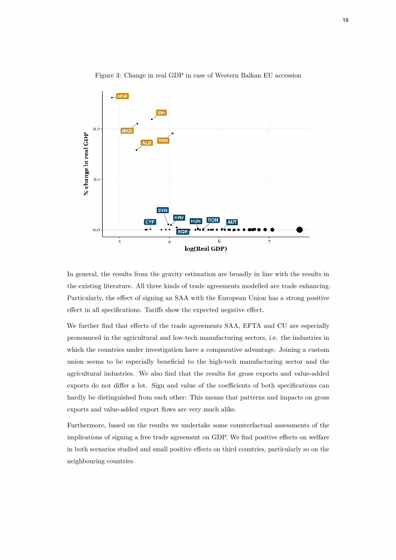
Figure 3: Change in real GDP in case of Western Balkan EU accession
In general, the results from the gravity estimation are broadly in line with the results in
the existing literature. All three kinds of trade agreements modelled are trade enhancing.
Particularly, the effect of signing an SAA with the European Union has a strong positive
effect in all specifications. Tariffs show the expected negative effect.
We further find that effects of the trade agreements SAA, EFTA and CU are especially
pronounced in the agricultural and low-tech manufacturing sectors, i.e. the industries in
which the countries under investigation have a comparative advantage. Joining a custom
union seems to be especially beneficial to the high-tech manufacturing sector and the
agricultural industries. We also find that the results for gross exports and value-added
exports do not differ a lot. Sign and value of the coefficients of both specifications can
hardly be distinguished from each other: This means that patterns and impacts on gross
exports and value-added export flows are very much alike.
Furthermore, based on the results we undertake some counterfactual assessments of the
implications of signing a free trade agreement on GDP. We find positive effects on welfare
in both scenarios studied and small positive effects on third countries, particularly so on the
neighbouring countries.
19
References
Anderson, J. E., Larch, M., & Yotov, Y. (2015). Estimating general equilibrium trade policy
effects: GE PPML.
Anderson, J. E., & Van Wincoop, E. (2003). Gravity with gravitas: A solution to the border
puzzle. The American Economic Review, 93 (1), 170–192.
Baier, S. L., & Bergstrand, J. H. (2007). Do free trade agreements actually increase members’
international trade? Journal of International Economics, 71 (1), 72–95.
Baldwin, R., & Taglioni, D. (2011). Gravity chains: Estimating bilateral trade flows when
parts and components trade is important (Tech. Rep.). National Bureau of Economic
Research.
Bouët, A., Decreux, Y., Fontagné, L., Jean, S., & Laborde, D. (2004). A consistent, ad-
valorem equivalent measure of applied protection across the world: The MAcMap-HS6
database.
Dowle, M., & Srinivasan, A. (2017). data.table: Extension of ‘data.frame‘ [Computer software
manual]. Retrieved from https://CRAN.R-project.org/package=data.table (R
package version 1.10.4)
Egger, P., & Larch, M. (2008). Interdependent preferential trade agreement memberships:
An empirical analysis. Journal of International Economics, 76 (2), 384–399.
Egger, P. H., & Nigai, S. (2015). Structural gravity with dummies only: Constrained
anova-type estimation of gravity models. Journal of International Economics, 97 (1),
86–99.
Eurostat. (2008). Eurostat manual of supply, use and input–output tables. Eurostat
Luxembourg.
Fally, T. (2015). Structural gravity and fixed effects. Journal of International Economics,
97 (1), 76–85.
Head, K. (2014). Gravity equations: Workhorse, toolkit, and cookbook. Handbook of
International Economics, 4 , 131.
Head, K., Mayer, T., & Ries, J. (2010). The erosion of colonial trade linkages after
independence. Journal of International Economics, 81 (1), 1–14.
Johnson, R. C., & Noguera, G. (2012). Accounting for intermediates: Production sharing
and trade in value added. Journal of International Economics, 86 (2), 224–236.
Larch, M., Wanner, J., Yotov, Y., & Zylkin, T. (2017). The currency union effect: A PPML
re-assessment with high-dimensional fixed effects.
Monastiriotis, V., Kallioras, D., & Petrakos, G. C. (2014). The regional impact of EU
association agreements: Lessons for the ENP from the CEE experience.
20
Pula, E. (2014). The trade impact of the kosovo-EU Stabilization and Association Agreement:
An assessment of outcomes and implications. A policy report by the group of legal
and political studies, No. 3.
R Core Team. (2017). R: A language and environment for statistical computing [Computer
software manual]. Vienna, Austria. Retrieved from https://www.R-project.org/
Sebastian, S. (2008). The Stabilisation and Association Process: Are EU inducements
failing in the Western Balkans. Fundación para las Relaciones Internacionales y el
Diálogo Exterior (FRIDE), Madrid.
Silva, J. S., & Tenreyro, S. (2006). The log of gravity. The Review of Economics and
Statistics, 88 (4), 641–658.
Silva, J. S., & Tenreyro, S. (2011). Further simulation evidence on the performance of the
Poisson Pseudo-Maximum Likelihood estimator. Economics Letters, 112 (2), 220–222.
Stadler, K., Steen-Olsen, K., & Wood, R. (2014). The ‘Rest of the World’ - Estimating
the economic structure of missing regions in global multi-regional input–output tables.
Economic Systems Research, 26 (3), 303–326.
Stehrer, R. (2012). Trade in Value Added and the Valued Added in trade. WIOD Working
Paper .
Streicher, G., & Stehrer, R. (2015). Whither Panama? Constructing a consistent and
balanced world SUT system including international trade and transport margins.
Economic Systems Research, 27 (2), 213–237.
Temurshoev, U., & Timmer, M. P. (2011). Joint estimation of supply and use tables. Papers
in Regional Science, 90 (4), 863–882.
Timmer, M. P., Dietzenbacher, E., Los, B., Stehrer, R., & Vries, G. J. (2015). An illustrated
user guide to the World Input–Output Database: The case of global automotive
production. Review of International Economics, 23 (3), 575–605.
Timmer, M. P., Los, B., Stehrer, R., & de Vries, G. J. (2016). Peak trade? An anatomy of
the global trade slowdown. GGDC Research Memorandum(162).
Yotov, Y. V., Piermartini, R., Monteiro, J.-A., & Larch, M. (2016). An advanced guide
to trade policy analysis: The structural gravity model. World Trade Organization,
Geneva.
Zahariadis, Y. (2007). The effects of the Albania-EU stabilization and association agreement:
Economic impact and social implications. London: Overseas Development Institute,
20 , 2007–2008.
21
A Appendix: Construction issues of the “wiiw Wider
Europe Multi-Country Input-Output Table”
A.1 Coverage
In the first phase the underlying data for the construction the multi-country input-output
tables (MC IOTs) have been collected and harmonized. Data on the European countries -
including all EU-28 Member States, Switzerland, Iceland and Norway, five Western Balkan
countries (Albania (AL), Bosnia and Herzegovina (BA), Montenegro (ME), Macedonia
(MK), Serbia (RS)) and the Ukraine (UA) - have been collected from Eurostat and national
sources. These data include time series of National Accounts data for gross output, value
added and intermediate inputs as well as total exports and imports. Further, benchmark
supply and use tables when available have been collected and harmonised. If available use
tables have been gathered both in basic and purchaser’s prices and import use tables (in
basic prices) have been collected as well. Furthermore, all these supply and use tables are
based on the newest classification of activities (NACE Rev. 2) and commodities (according
to CPA 2008) and were compiled according to the recent methodology of the Systems of
National Accounts (SNA2008/ESA2010). The only exception to this is Montenegro which
has published SNA data according to ESA 1995 only.
Data for the other thirteen biggest economies outside Europe – including Australia (AU),
Brazil (BR), Canada (CA), China (CN), Indonesia (ID), India (IN), Japan (JP), Korea
(KR), Mexiko (MX), Russia (RU), Turkey (TR), Taiwan (TW) and the United States (US) -
have been taken over from the WIOD database (see Timmer et al. (2015) for documentation).
The WIOD release 2016 also covers the EU-28 countries. However, data for these countries
have been computed and updated in the same way as for the other countries; particularly
information from purchaser’s and basic price tables and import use tables have been taken
into account. The advantage is that our slightly different methodological approach allows to
us to effectively make use of the full information set by country provided by Eurostat and
does less rely on assumptions about, e.g., the import structure of a country. Compared to
the data in WIOD this has some implications on the level of export data and export/GDP
ratios, the treatment of re-exports and a different assumption concerning the allocation of
intermediate trade in services.
Based on these available benchmark supply and use tables (SUTs) and system of national
accounts data (SNA) the so-called “SUT-RAS” algorithm (see Temurshoev and Timmer
(2011)) has been applied to back- and forecast SUTs according to the most recently available
22
SNA data. It should be noted that – differently to the WIOD approach – in this exercise
the full information from available datasets (i.e. tables in purchaser and basic prices, import
use tables) have been used to construct a consistent time series.
The data for these three country groups have been harmonised across countries and time to
make them as consistent and comparable as possible: SUTs and SNA data were available
on the different level of disaggregation for different countries. While all Eurostat-based
data is available for 64 industries, data for the West Balkan countries are only available for
about 20 to 30 industries. We chose to use an industry aggregation of 32 industries. For
countries which reported more aggregated data we applied shares from more detailed SUT
data or used shares of countries with similar industry structure. Therefore, due to these data
constraints on industry details in some of the interesting countries the final version of the
data comprises 32 industries (see Appendix Table A.1). Furthermore, missing information
in the national SUTs has been imputed by various steps: Missing import use tables (or
valuation matrices) have been estimated from the total use tables, missing product data in
either the supply or use table have also been imputed.
The resulting set of data is documented in Appendix Table A.2 which provides information
on raw data (which still had to be harmonised) and estimated time series. The final database
therefore covers 50 countries, 32 industries and over the period 2005 to 2014. Some more
details concerning construction and assumptions are provided below.
A.2 Benchmarking and estimation of SUTs
Based on these data we have benchmarked SUTs to the most recent SNA data and estimated
SUTs for years where this information hasn’t been available (again on the basis of the recent
SNA data) using the SUT-RAS algorithm as outlined in Temurshoev and Timmer (2011).
This resulted in the coverage as presented in Appendix Table A.2.
1. A dark-green colour indicates that for these years SUTs according to ESA2010 and
corresponding to NACE Rev. 2 / CPA 2008 have been available and were only
benchmarked to the most recent SNA data. In these cases countries also provide
valuation matrices - for trade and transport margins (TTM) and taxes less subsidies
(TLS) – implying that use tables are available both in purchasers’ prices (USEp) and
basic prices (USEb). The countries in this category are also reporting import use
tables.
2. For a second set of countries – indicated in dark-blue – SUTs are available according
23
to ESA2010 and corresponding to NACE Rev. 2 / CPA 2008 which have been
benchmarked to recent SNA data. Again these countries provide valuation matrices,
however import use tables have to be estimated.
3. The third group of countries – indicated in orange – provide SUTs again according
to ESA2010 and corresponding to NACE Rev. 2 / CPA 2008 but without valuation
matrices, i.e. the use tables are only reported in basic prices. Thus for these countries
use tables in purchaser prices have to be estimated using data on trade and transport
margins and taxes.
4. Finally, for five countries – Bosnia and Herzegovina (BA), Iceland (IS), Montenegro
(ME), Serbia (RS) and Ukraine (UA) – only SNA data are available. Montenegro and
Bosnia & Herzegovina published the SNA data using ESA 1995 methodology, while
the data for the other three countries is compiled according to ESA 2010. To estimate
the SUTs for these countries, we assume that their economic structure is comparable
to another country and use those SUTs to estimate the whole SUT time series. The
SUT replacements have been indicated by the country codes, as can be seen in Table
A.2.
Based on these harmonised benchmark SUTs we then used the SUT-RAS algorithm and
SNA data to estimate a whole time series of SUTs from 2005 to 2014.
A.3 Trade data
The next step that followed was the construction of international SUTs, i.e. the breakdown
of the import use tables by source country. For this purpose detailed trade data from UN
COMTRADE for trade in goods and from the UN Services Trade Database for trade in
services have been collected. Both data sources have been harmonised and reconciled with
the information in the SUTs. Data on trade in services are patchy, which was another reason
for us to aggregate the data to 32 industries, to remedy some of the quality problems that
come with even more disaggregated data.
A.4 Estimating Rest-of-the-World region and inter-country IOTs
Additionally, a Rest-of-World country is included in the international SUTs. The structure
of the SUTs for Rest-of-World country is based on the average of all 50 countries in the
database (see Stadler, Steen-Olsen, and Wood (2014)) and benchmarked to GDP data of the
remaining 150 countries (taken from UN) so that we finally arrive at picture of the world’s
24

economic structure that is as accurate as possible. This is again done differently as in the
WIOD approach where the Rest-of-World has been estimated only after the construction of
the international input-output table (see also Streicher and Stehrer (2015) on this).
The resulting international SUTs were then used to derive symmetric, industry-by-industry
Input-Output Tables using the assumption of a fixed sales structure. This method of
calculating input-output tables has the two advantages: First, it seems the least restrictive
to us, and second, it does not produce negative elements in the resulting intermediates
matrix, thus does not require any further adjustments.
25
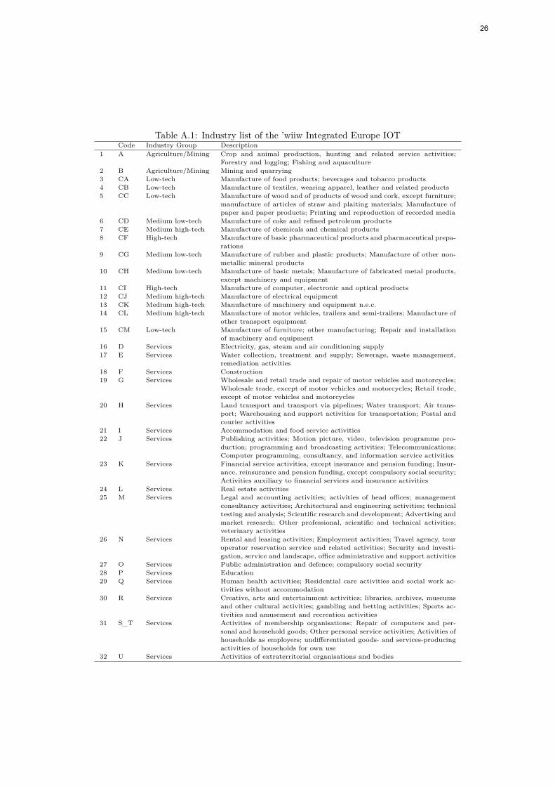
Table A.1: Industry list of the ’wiiw Integrated Europe IOTCode Industry Group Description
1 A Agriculture/Mining Crop and animal production, hunting and related service activities;Forestry and logging; Fishing and aquaculture
2 B Agriculture/Mining Mining and quarrying3 CA Low-tech Manufacture of food products; beverages and tobacco products4 CB Low-tech Manufacture of textiles, wearing apparel, leather and related products5 CC Low-tech Manufacture of wood and of products of wood and cork, except furniture;
manufacture of articles of straw and plaiting materials; Manufacture ofpaper and paper products; Printing and reproduction of recorded media
6 CD Medium low-tech Manufacture of coke and refined petroleum products7 CE Medium high-tech Manufacture of chemicals and chemical products8 CF High-tech Manufacture of basic pharmaceutical products and pharmaceutical prepa-
rations9 CG Medium low-tech Manufacture of rubber and plastic products; Manufacture of other non-
metallic mineral products10 CH Medium low-tech Manufacture of basic metals; Manufacture of fabricated metal products,
except machinery and equipment11 CI High-tech Manufacture of computer, electronic and optical products12 CJ Medium high-tech Manufacture of electrical equipment13 CK Medium high-tech Manufacture of machinery and equipment n.e.c.14 CL Medium high-tech Manufacture of motor vehicles, trailers and semi-trailers; Manufacture of
other transport equipment15 CM Low-tech Manufacture of furniture; other manufacturing; Repair and installation
of machinery and equipment16 D Services Electricity, gas, steam and air conditioning supply17 E Services Water collection, treatment and supply; Sewerage, waste management,
remediation activities18 F Services Construction19 G Services Wholesale and retail trade and repair of motor vehicles and motorcycles;
Wholesale trade, except of motor vehicles and motorcycles; Retail trade,except of motor vehicles and motorcycles
20 H Services Land transport and transport via pipelines; Water transport; Air trans-port; Warehousing and support activities for transportation; Postal andcourier activities
21 I Services Accommodation and food service activities22 J Services Publishing activities; Motion picture, video, television programme pro-
duction; programming and broadcasting activities; Telecommunications;Computer programming, consultancy, and information service activities
23 K Services Financial service activities, except insurance and pension funding; Insur-ance, reinsurance and pension funding, except compulsory social security;Activities auxiliary to financial services and insurance activities
24 L Services Real estate activities25 M Services Legal and accounting activities; activities of head offices; management
consultancy activities; Architectural and engineering activities; technicaltesting and analysis; Scientific research and development; Advertising andmarket research; Other professional, scientific and technical activities;veterinary activities
26 N Services Rental and leasing activities; Employment activities; Travel agency, touroperator reservation service and related activities; Security and investi-gation, service and landscape, office administrative and support activities
27 O Services Public administration and defence; compulsory social security28 P Services Education29 Q Services Human health activities; Residential care activities and social work ac-
tivities without accommodation30 R Services Creative, arts and entertainment activities; libraries, archives, museums
and other cultural activities; gambling and betting activities; Sports ac-tivities and amusement and recreation activities
31 S_T Services Activities of membership organisations; Repair of computers and per-sonal and household goods; Other personal service activities; Activities ofhouseholds as employers; undifferentiated goods- and services-producingactivities of households for own use
32 U Services Activities of extraterritorial organisations and bodies
26
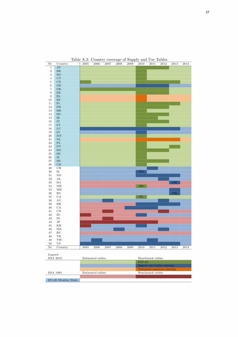
Table A.2: Country coverage of Supply and Use TablesNr Country 2005 2006 2007 2008 2009 2010 2011 2012 2013 20141 AT2 BE3 BG4 CY5 CZ6 DE7 DK8 EE9 EL
10 ES11 FI12 FR13 HR14 HU15 IE16 IT17 LT18 LU19 LV20 MT21 NL22 PL23 PT24 RO25 SE26 SI27 SK28 UK29 CH30 IS NO31 NO32 AL33 BA MK34 ME HR35 MK36 RS MK37 UA PL38 AU39 BR40 CA41 CN42 ID43 IN44 JP45 KR46 MX47 RU48 TR49 TW50 USNr Country 2005 2006 2007 2008 2009 2010 2011 2012 2013 2014
Legend:ESA 2010 Estimated tables Benchmark tables
Full setImport use tables missingValuation matrices missing
ESA 1995 Estimated tables Benchmark tables
EU-28 Member State
27
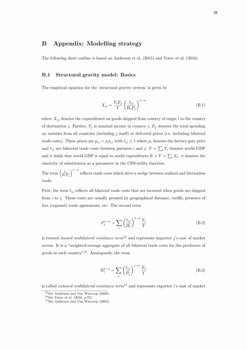
B Appendix: Modelling strategy
The following short outline is based on Anderson et al. (2015) and Yotov et al. (2016).
B.1 Structural gravity model: Basics
The empirical equation for the ’structural gravity system’ is given by
Xij = YiEjY
(tij
ΠiPj
)1−σ
(B.1)
where Xij denotes the expenditures on goods shipped from country of origin i to the country
of destination j. Further, Yj is nominal income in country j, Ej denotes the total spending
on varieties from all countries (including j itself) at delivered prices (i.e. including bilateral
trade costs). These prices are pij = pitij with tij ≥ 1 where pi denotes the factory-gate price
and tij are bilateral trade costs between partners i and j. Y =∑i Yi denotes world GDP
and it holds that world GDP is equal to world expenditures E = Y =∑iEi. σ denotes the
elasticity of substitution as a parameter in the CES-utility function.
The term(
tijΠiPj
)1−σreflects trade costs which drive a wedge between realized and frictionless
trade.
First, the term tij reflects all bilateral trade costs that are incurred when goods are shipped
from i to j. These costs are usually proxied by geographical distance, tariffs, presence of
free (regional) trade agreements, etc. The second term
P 1−σj =
∑i
(tijΠi
)1−σYiY
(B.2)
is termed inward multilateral resistance term15 and represents importer j’s ease of market
access. It is a “weighted-average aggregate of all bilateral trade costs for the producers of
goods in each country”16. Analogously, the term
Π1−σi =
∑j
(tijPj
)1−σEjY
(B.3)
is called outward multilateral resistance term17 and represents exporter i’s ease of market15See Anderson and Van Wincoop (2003).16See Yotov et al. (2016, p.72)17See Anderson and Van Wincoop (2003).
28
access.
Further, the term
pi =∑j
(YiY
) 11−σ 1
αiΠi(B.4)
denotes the factory-gate price for each variety of goods in country i. Finally,
Ei = ϕiYi = ϕipiQi (B.5)
denotes total expenditures in country i with Qi denoting the endowment or quantity supplied
of each variety of goods in country i. Here, ϕ denotes the relation between value of output
and aggregate expenditure. If ϕ = 1 the economy is characterised by balanced trade, if
ϕ > 1 the country faces a trade deficit (expenditures are larger than value of output) and if
ϕ < 1 the country faces a trade surplus.
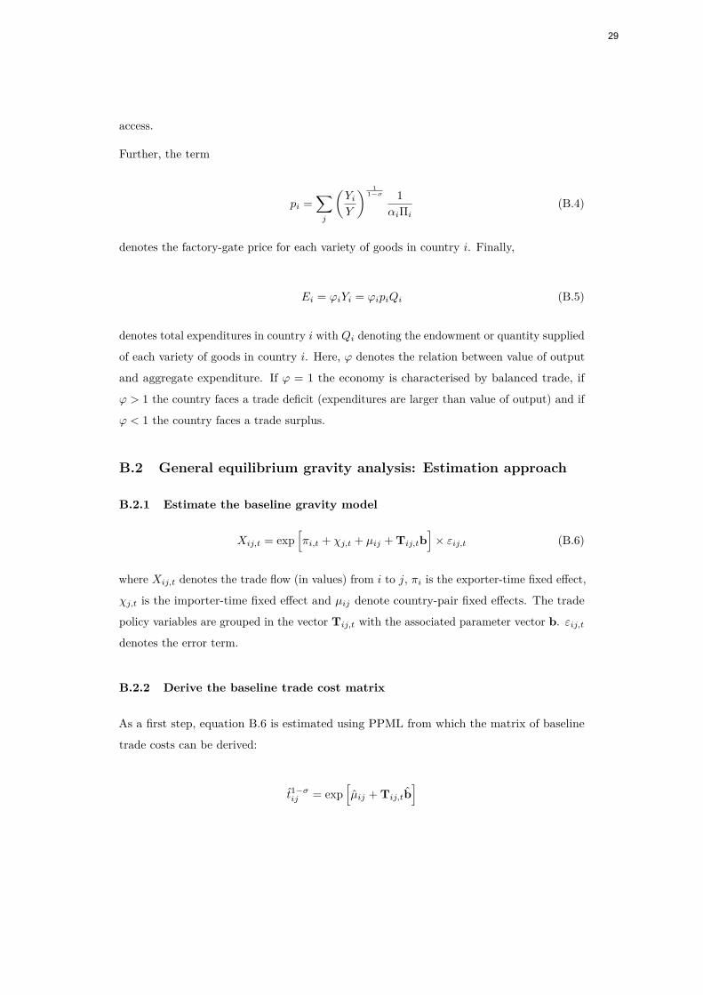
B.2 General equilibrium gravity analysis: Estimation approach
B.2.1 Estimate the baseline gravity model
Xij,t = exp[πi,t + χj,t + µij + Tij,tb
]× εij,t (B.6)
where Xij,t denotes the trade flow (in values) from i to j, πi is the exporter-time fixed effect,
χj,t is the importer-time fixed effect and µij denote country-pair fixed effects. The trade
policy variables are grouped in the vector Tij,t with the associated parameter vector b. εij,tdenotes the error term.
B.2.2 Derive the baseline trade cost matrix
As a first step, equation B.6 is estimated using PPML from which the matrix of baseline
trade costs can be derived:
t̂1−σij = exp
[µ̂ij + Tij,tb̂
]
29
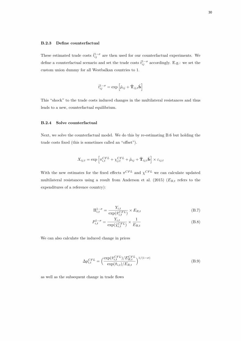
B.2.3 Define counterfactual
These estimated trade costs t̂1−σij are then used for our counterfactual experiments. We
define a counterfactual scenario and set the trade costs t̃1−σij accordingly. E.g.: we set the
custom union dummy for all Westbalkan countries to 1.
t̃1−σij = exp
[µ̂ij + T̃ij,tb̂
]This “shock” to the trade costs induced changes in the multilateral resistances and thus
leads to a new, counterfactual equilibrium.
B.2.4 Solve counterfactual
Next, we solve the counterfactual model. We do this by re-estimating B.6 but holding the
trade costs fixed (this is sometimes called an “offset”).
Xij,t = exp[πCFLi,t + χCFLj,t + µ̂ij + T̃ij,tb̂
]× εij,t
With the new estimates for the fixed effects πCFL and χCFL we can calculate updated
multilateral resistances using a result from Anderson et al. (2015) (ER,t refers to the
expenditures of a reference country):
Π1−σi,t = Yi,t
exp(π̂CFLi,t )× ER,t (B.7)
P 1−σi,t = Yi,t
exp(χ̂CFLi,t )× 1ER,t
(B.8)
We can also calculate the induced change in prices
∆pCFLi,t =(exp(π̂CFLi,t )/ECFLR,t
exp(π̂i,t)/ER,t
)1/(1−σ)(B.9)
as well as the subsequent change in trade flows
30
XCFLij,t =
[t̂1−σij
]CFLt̂1−σij
×Y CFLi,t ECFLj,t
Yi,tEj,t×
Π1−σi,t[
Π1−σi,t
]CFL ×P 1−σj,t[
P 1−σj,t
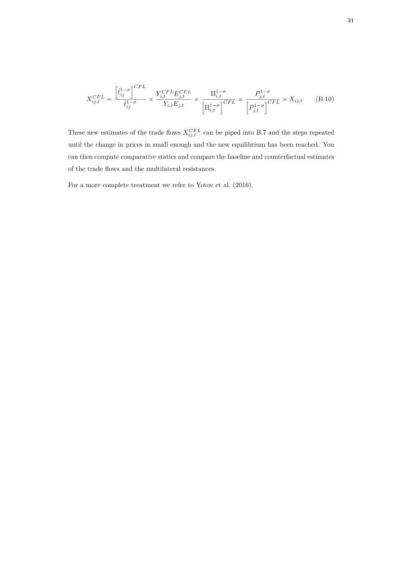
]CFL ×Xij,t (B.10)
These new estimates of the trade flows XCFLij,t can be piped into B.7 and the steps repeated
until the change in prices in small enough and the new equilibrium has been reached. You
can then compute comparative statics and compare the baseline and counterfactual estimates
of the trade flows and the multilateral resistances.
For a more complete treatment we refer to Yotov et al. (2016).
31
C Appendix: Using gross output as mass variable
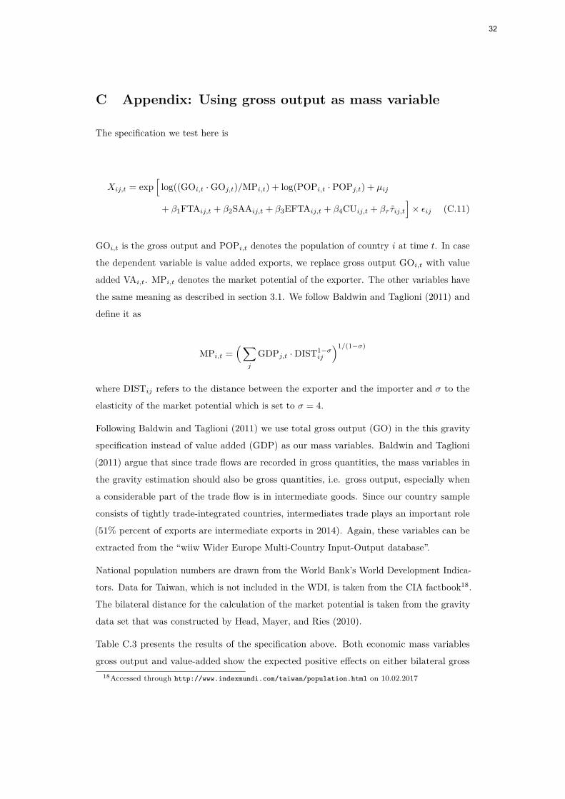
The specification we test here is
Xij,t = exp[
log((GOi,t · GOj,t)/MPi,t) + log(POPi,t · POPj,t) + µij
+ β1FTAij,t + β2SAAij,t + β3EFTAij,t + β4CUij,t + βτ τ̃ij,t
]× εij (C.11)
GOi,t is the gross output and POPi,t denotes the population of country i at time t. In case
the dependent variable is value added exports, we replace gross output GOi,t with value
added VAi,t. MPi,t denotes the market potential of the exporter. The other variables have
the same meaning as described in section 3.1. We follow Baldwin and Taglioni (2011) and
define it as
MPi,t =(∑
j
GDPj,t · DIST1−σij
)1/(1−σ)
where DISTij refers to the distance between the exporter and the importer and σ to the
elasticity of the market potential which is set to σ = 4.
Following Baldwin and Taglioni (2011) we use total gross output (GO) in the this gravity
specification instead of value added (GDP) as our mass variables. Baldwin and Taglioni
(2011) argue that since trade flows are recorded in gross quantities, the mass variables in
the gravity estimation should also be gross quantities, i.e. gross output, especially when
a considerable part of the trade flow is in intermediate goods. Since our country sample
consists of tightly trade-integrated countries, intermediates trade plays an important role
(51% percent of exports are intermediate exports in 2014). Again, these variables can be
extracted from the “wiiw Wider Europe Multi-Country Input-Output database”.
National population numbers are drawn from the World Bank’s World Development Indica-
tors. Data for Taiwan, which is not included in the WDI, is taken from the CIA factbook18.
The bilateral distance for the calculation of the market potential is taken from the gravity
data set that was constructed by Head, Mayer, and Ries (2010).
Table C.3 presents the results of the specification above. Both economic mass variables
gross output and value-added show the expected positive effects on either bilateral gross18Accessed through http://www.indexmundi.com/taiwan/population.html on 10.02.2017
32
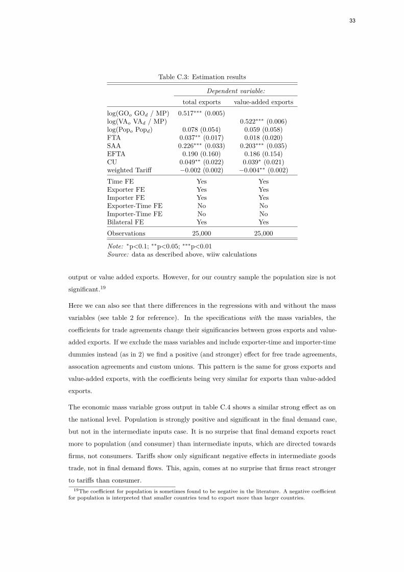
Table C.3: Estimation results
Dependent variable:total exports value-added exports
log(GOo GOd / MP) 0.517∗∗∗ (0.005)log(VAo VAd / MP) 0.522∗∗∗ (0.006)log(Popo Popd) 0.078 (0.054) 0.059 (0.058)FTA 0.037∗∗ (0.017) 0.018 (0.020)SAA 0.226∗∗∗ (0.033) 0.203∗∗∗ (0.035)EFTA 0.190 (0.160) 0.186 (0.154)CU 0.049∗∗ (0.022) 0.039∗ (0.021)weighted Tariff −0.002 (0.002) −0.004∗∗ (0.002)Time FE Yes YesExporter FE Yes YesImporter FE Yes YesExporter-Time FE No NoImporter-Time FE No NoBilateral FE Yes YesObservations 25,000 25,000
Note: ∗p<0.1; ∗∗p<0.05; ∗∗∗p<0.01Source: data as described above, wiiw calculations
output or value added exports. However, for our country sample the population size is not
significant.19
Here we can also see that there differences in the regressions with and without the mass
variables (see table 2 for reference). In the specifications with the mass variables, the
coefficients for trade agreements change their significancies between gross exports and value-
added exports. If we exclude the mass variables and include exporter-time and importer-time
dummies instead (as in 2) we find a positive (and stronger) effect for free trade agreements,
assocation agreements and custom unions. This pattern is the same for gross exports and
value-added exports, with the coefficients being very similar for exports than value-added
exports.
The economic mass variable gross output in table C.4 shows a similar strong effect as on
the national level. Population is strongly positive and significant in the final demand case,
but not in the intermediate inputs case. It is no surprise that final demand exports react
more to population (and consumer) than intermediate inputs, which are directed towards
firms, not consumers. Tariffs show only significant negative effects in intermediate goods
trade, not in final demand flows. This, again, comes at no surprise that firms react stronger
to tariffs than consumer.19The coefficient for population is sometimes found to be negative in the literature. A negative coefficient
for population is interpreted that smaller countries tend to export more than larger countries.
33
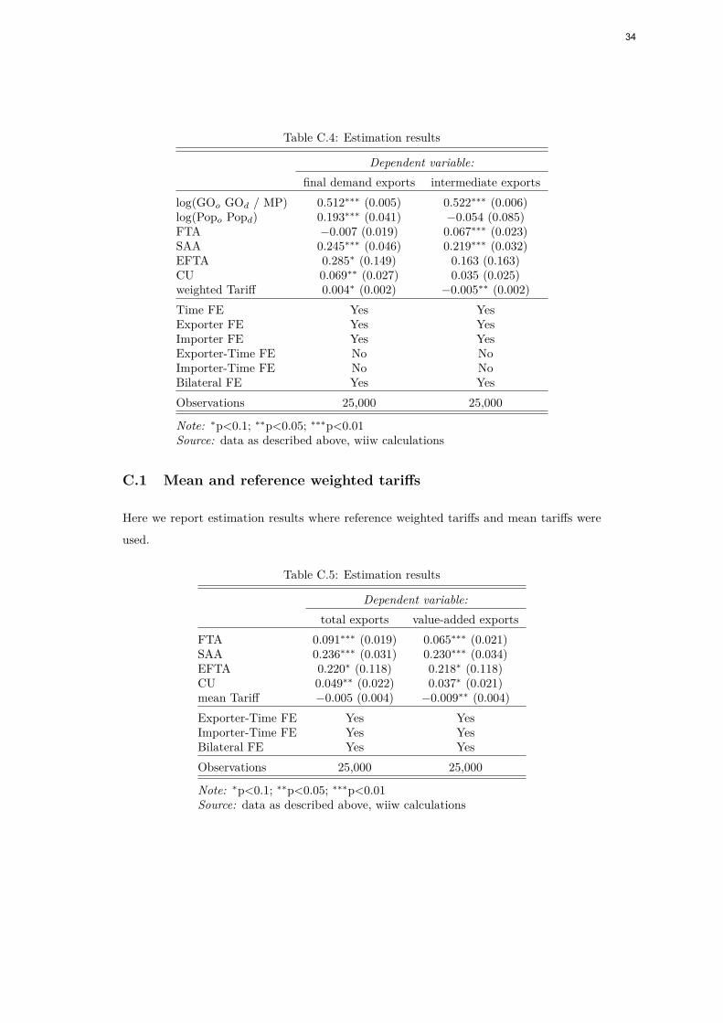
Table C.4: Estimation results
Dependent variable:final demand exports intermediate exports
log(GOo GOd / MP) 0.512∗∗∗ (0.005) 0.522∗∗∗ (0.006)log(Popo Popd) 0.193∗∗∗ (0.041) −0.054 (0.085)FTA −0.007 (0.019) 0.067∗∗∗ (0.023)SAA 0.245∗∗∗ (0.046) 0.219∗∗∗ (0.032)EFTA 0.285∗ (0.149) 0.163 (0.163)CU 0.069∗∗ (0.027) 0.035 (0.025)weighted Tariff 0.004∗ (0.002) −0.005∗∗ (0.002)Time FE Yes YesExporter FE Yes YesImporter FE Yes YesExporter-Time FE No NoImporter-Time FE No NoBilateral FE Yes YesObservations 25,000 25,000
Note: ∗p<0.1; ∗∗p<0.05; ∗∗∗p<0.01Source: data as described above, wiiw calculations
C.1 Mean and reference weighted tariffs
Here we report estimation results where reference weighted tariffs and mean tariffs were
used.
Table C.5: Estimation results
Dependent variable:total exports value-added exports
FTA 0.091∗∗∗ (0.019) 0.065∗∗∗ (0.021)SAA 0.236∗∗∗ (0.031) 0.230∗∗∗ (0.034)EFTA 0.220∗ (0.118) 0.218∗ (0.118)CU 0.049∗∗ (0.022) 0.037∗ (0.021)mean Tariff −0.005 (0.004) −0.009∗∗ (0.004)Exporter-Time FE Yes YesImporter-Time FE Yes YesBilateral FE Yes YesObservations 25,000 25,000
Note: ∗p<0.1; ∗∗p<0.05; ∗∗∗p<0.01Source: data as described above, wiiw calculations
34
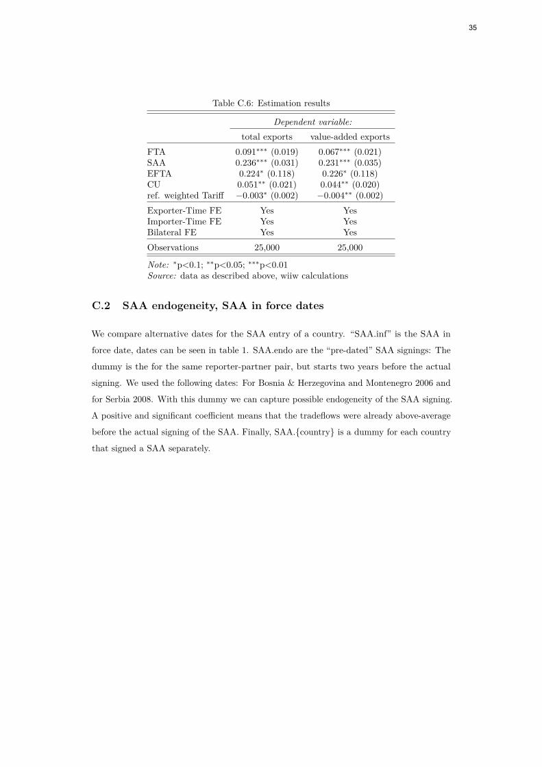
Table C.6: Estimation results
Dependent variable:total exports value-added exports
FTA 0.091∗∗∗ (0.019) 0.067∗∗∗ (0.021)SAA 0.236∗∗∗ (0.031) 0.231∗∗∗ (0.035)EFTA 0.224∗ (0.118) 0.226∗ (0.118)CU 0.051∗∗ (0.021) 0.044∗∗ (0.020)ref. weighted Tariff −0.003∗ (0.002) −0.004∗∗ (0.002)Exporter-Time FE Yes YesImporter-Time FE Yes YesBilateral FE Yes YesObservations 25,000 25,000
Note: ∗p<0.1; ∗∗p<0.05; ∗∗∗p<0.01Source: data as described above, wiiw calculations
C.2 SAA endogeneity, SAA in force dates
We compare alternative dates for the SAA entry of a country. “SAA.inf” is the SAA in
force date, dates can be seen in table 1. SAA.endo are the “pre-dated” SAA signings: The
dummy is the for the same reporter-partner pair, but starts two years before the actual
signing. We used the following dates: For Bosnia & Herzegovina and Montenegro 2006 and
for Serbia 2008. With this dummy we can capture possible endogeneity of the SAA signing.
A positive and significant coefficient means that the tradeflows were already above-average
before the actual signing of the SAA. Finally, SAA.{country} is a dummy for each country
that signed a SAA separately.
35
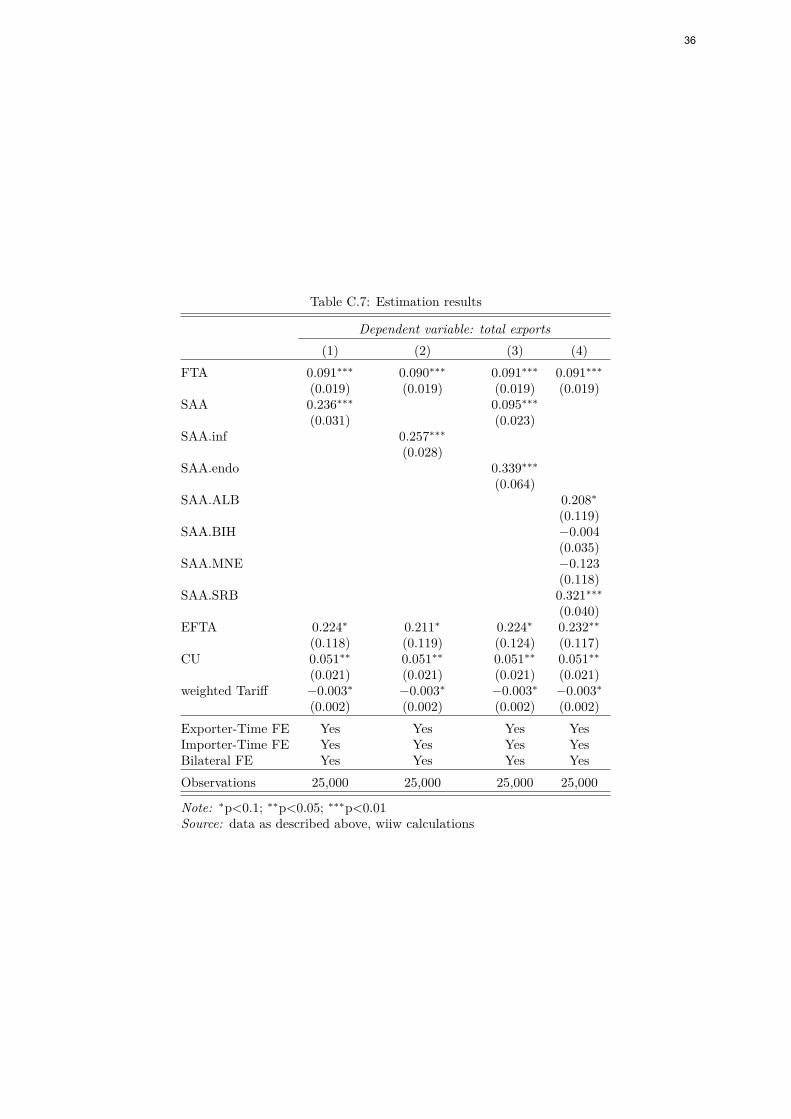
Table C.7: Estimation results
Dependent variable: total exports(1) (2) (3) (4)
FTA 0.091∗∗∗ 0.090∗∗∗ 0.091∗∗∗ 0.091∗∗∗
(0.019) (0.019) (0.019) (0.019)SAA 0.236∗∗∗ 0.095∗∗∗
(0.031) (0.023)SAA.inf 0.257∗∗∗
(0.028)SAA.endo 0.339∗∗∗
(0.064)SAA.ALB 0.208∗
(0.119)SAA.BIH −0.004
(0.035)SAA.MNE −0.123
(0.118)SAA.SRB 0.321∗∗∗
(0.040)EFTA 0.224∗ 0.211∗ 0.224∗ 0.232∗∗
(0.118) (0.119) (0.124) (0.117)CU 0.051∗∗ 0.051∗∗ 0.051∗∗ 0.051∗∗
(0.021) (0.021) (0.021) (0.021)weighted Tariff −0.003∗ −0.003∗ −0.003∗ −0.003∗
(0.002) (0.002) (0.002) (0.002)Exporter-Time FE Yes Yes Yes YesImporter-Time FE Yes Yes Yes YesBilateral FE Yes Yes Yes YesObservations 25,000 25,000 25,000 25,000
Note: ∗p<0.1; ∗∗p<0.05; ∗∗∗p<0.01Source: data as described above, wiiw calculations
36
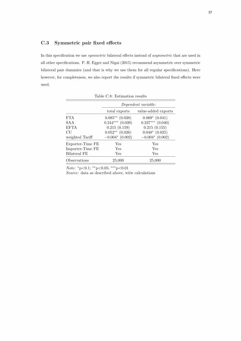
C.3 Symmetric pair fixed effects
In this specification we use symmetric bilateral effects instead of asymmetric that are used in
all other specifications. P. H. Egger and Nigai (2015) recommend asymmetric over symmetric
bilateral pair dummies (and that is why we use them for all regular specifications). Here
however, for completeness, we also report the results if symmetric bilateral fixed effects were
used.
Table C.8: Estimation results
Dependent variable:total exports value-added exports
FTA 0.085∗∗ (0.038) 0.069∗ (0.041)SAA 0.244∗∗∗ (0.039) 0.237∗∗∗ (0.040)EFTA 0.215 (0.159) 0.215 (0.155)CU 0.052∗∗ (0.026) 0.048∗ (0.025)weighted Tariff −0.004∗ (0.002) −0.004∗ (0.002)Exporter-Time FE Yes YesImporter-Time FE Yes YesBilateral FE Yes YesObservations 25,000 25,000
Note: ∗p<0.1; ∗∗p<0.05; ∗∗∗p<0.01Source: data as described above, wiiw calculations
37

For current updates and summaries see also wiiw's website at www.wiiw.ac.at
No. 148 Oliver Reiter and Robert Stehrer: Trade Policies and Integration of the Western Balkans, May 2018
No. 147 Philipp Heimberger: The Dynamic Effects of Fiscal Consolidation Episodes on Income Inequality: Evidence for
17 OECD Countries over 1978-2013, April 2018
No. 146 Mahdi Ghodsi: The Impact of Chinese Technical Barriers to Trade on its Manufacturing Imports, March 2018
No. 145 Amat Adarov: Financial Cycles Around the World, March 2018
No. 144 Mario Holzner: Corporatism and the Labour Income Share. Econometric Investigation into the Impact of Institutions
on the Wage Share of Industrialised Nations, March 2018
No. 143 Claudius Gräbner, Philipp Heimberger, Jakob Kapeller, Bernhard Schütz: Structural Change in Times of Increasing
Openness: Assessing Path Dependency in European Economic Integration, March 2018
No. 142 Loredana Fattorini, Mahdi Ghodsi and Armando Rungi: Cohesion Policy Meets Heterogeneous Firms, March 2018
No. 141 Neil Foster-McGregor, Michael Landesmann and Isilda Mara: Migration and FDI Flows, March 2018
No. 140 Amat Adarov: Financial Cycles in Credit, Housing and Capital Markets: Evidence from Systemic Economies,
December 2017
No. 139 Eddy Bekkers, Michael Landesmann and Indre Macskasi: Trade in Services versus Trade in Manufactures: The
Relation between the Role of Tacit Knowledge, the Scope for Catch-up, and Income Elasticity, December 2017
No. 138 Roman Stöllinger: Global Value Chains and Structural Upgrading, September 2017
No. 137 Stefan Jestl, Mathias Moser and Anna K. Raggl:
Pushes Internal Migration in Austria, September 2017
No. 136 Claudius Gräbner, Philipp Heimberger, Jakob Kapeller and Bernhard Schütz: Is Europe Disintegrating?
Macroeconomic Divergence, Structural Polarisation, Trade and Fragility, September 2017
No. 135 Mahdi Ghodsi and Robert Stehrer: EU Trade Regulations and Imports of Hygienic Poultry, April 2017
No. 134 Roman Stöllinger: Tradability of Output and the Current Account: An Empirical Investigation for Europe,
January 2017
No. 133 Tomislav Globan: Financial Supply Index and Financial Supply Cycles in New EU Member States, December 2016
No. 132 Mahdi Ghodsi, Julia Grübler and Robert Stehrer: Import Demand Elasticities Revisited, November 2016
No. 131 Leon Podkaminer: Has Trade Been Driving Global Economic Growth?, October 2016
No. 130 Philipp Heimberger: Did Fiscal Consolidation Cause the Double-Dip Recession in the Euro Area?, October 2016
No. 129 Julia Grübler, Mahdi Ghodsi and Robert Stehrer: Estimating Importer-Specific Ad Valorem Equivalents of Non-
Tariff Measures, September 2016
No. 128 Sebastian Leitner and Robert Stehrer: Development of Public Spending Structures in the EU Member States:
Social Investment and its Impact on Social Outcomes, August 2016
No. 127 Roman Stöllinger: Structural Change and Global Value Chains in the EU, July 2016
No. 126 Jakob Kapeller, Michael Landesmann, Franz X. Mohr and Bernhard Schütz: Government Policies and Financial
Crises: Mitigation, Postponement or Prevention?, May 2016
No. 125 Sandra M. Leitner and Robert Stehrer: The Role of Financial Constraints for Different Innovation Strategies:
Evidence for CESEE and FSU Countries, April 2016
No. 124 Sandra M. Leitner: Choosing the Right Partner: R&D Cooperations and Innovation Success, February 2016
No. 123 Michael Landesmann, Sandra M. Leitner and Robert Stehrer: Changing Patterns in M&E-Investment-Based
Innovation Strategies in CESEE and FSU Countries: From Financial Normalcy to the Global Financial Crisis,
February 2016
No. 122 Sebastian Leitner: Drivers of Wealth Inequality in Euro-Area Countries. The Effect of Inheritance and Gifts on
Household Gross and Net Wealth Distribution Analysed by Applying the Shapley Value Approach to
Decomposition, January 2016
No. 121 Roman Stöllinger: Agglomeration and FDI: Bringing International Production Linkages into the Picture,
December 2015
No. 120 Michael Landesmann and Sandra M. Leitner: Intra-EU Mobility and Push and Pull Factors in EU Labour Markets:
Estimating a Panel VAR Model, August 2015
No. 119 Michael Landesmann and Sandra M. Leitner: Labour Mobility of Migrants and Natives in the European Union:
Greasing of the Wheel Effect' of Migrants, August 2015
No. 118 Johannes Pöschl and Katarina Valkova: Welfare State Regimes and Social Determinants of Health in Europe,
July 2015
No. 117 Mahdi Ghodsi: Distinguishing Between Genuine and Non-Genuine Reasons for Imposing TBTs; A Proposal Based
on Cost Benefit Analysis. July 2015
No. 116 Mahdi Ghodsi: Role of Specific Trade Concerns on TBT in the Import of Products to EU, USA, and China.
June 2015

IMPRESSUM
Herausgeber, Verleger, Eigentümer und Hersteller:
Wien 6, Rahlgasse 3
ZVR-Zahl: 329995655
Postanschrift: A 1060 Wien, Rahlgasse 3, Tel: [+431] 533 66 10, Telefax: [+431] 533 66 10 50
Internet Homepage: www.wiiw.ac.at
Nachdruck nur auszugsweise und mit genauer Quellenangabe gestattet.
Offenlegung nach § 25 Mediengesetz: Medieninhaber (Verleger): Verein "Wiener Institut für
Internationale Wirtschaftsvergleiche", A 1060 Wien, Rahlgasse 3. Vereinszweck: Analyse der
wirtschaftlichen Entwicklung der zentral- und osteuropäischen Länder sowie anderer
Transformationswirtschaften sowohl mittels empirischer als auch theoretischer Studien und ihre
Veröffentlichung; Erbringung von Beratungsleistungen für Regierungs- und Verwaltungsstellen,
Firmen und Institutionen.