WiFeS data reduction - draft manual

November 1, 2009

The WiFeS IRAF package consists of a set of IRAF CL scripts that can be used to process raw WiFeSintegral-field spectroscopic data to calibrate and remove instrumental/atmospheric effects from thedata and construct a 3D data set. Descriptions of the individual tasks can be found in their help files(the command ‘cl> help wifes’ lists those tasks with associated help files), and those of the subsidiarytasks that are used.

** The help files contained in the package are out of date and may contain some incorrect or incon-sistent information - please refer to this document first - 31/10/09.

1 Installing the wifes IRAF package

The instructions below are for installing a new version of the external wifes package on your system.

1. Download the current IRAF WiFeS package from the ANU/RSAA ftp site: the package is tem-porarily available from http://www.mso.anu.edu.au/~cfarage/ftp/wifes_package/. TheWiFeS package contains IRAF scripts, data files, some standard calibration data and docu-mentation files. Extract the subfolders and files to a location on your local system where usershave read and execute permissions.

2. The WiFeS package scripts rely on tasks in the Gemini IRAF package (particularly the gem-ini.gnirs and gemini.nifs sub-packages), which therefore need be installed before the WiFeSscripts can be used. Gemini version 1.9.1 is required, and is available, with installation instruc-tions, from: http://www.gemini.edu/sciops/data/dataSoftware.html. (Note: there is nowa PyRAF-compatible version of the Gemini package - v1.10, however the WiFeS package is notcompatible with PyRAF and has only been minimally tested with the new version in the CL)

3. To install the WiFeS package, you need to set some package-level variables. This can be doneusing either of the following options:

(a) Adding the following lines to your iraf$hlib/extern.pkg file (this will cause wifes to be listedas an available package when IRAF is loaded)

set wifes = /path/to/wifes/scripts/task wifes.pkg = wifes$wifes.cltask $expand $tr = $foreign

1

and in the statement setting the parameter helpdb in that file, add between the quotationmarks of the value:

,wifes$helpdb.mip

(b) Including the following lines in your login.cl or loginuser.cl file (in this case the package willnot be printed in the list of available packages at startup):

set wifes = “/path/to/wifes/scripts/”task wifes.pkg = “wifes$wifes.cl”task $expand $tr = “$foreign”reset helpdb = (envget( “helpdb”) // “,wifes$helpdb.mip”)

2 Setting up for data reduction

It is assumed here that you are already familiar with the basic use of IRAF - you can refer to onlinetutorials (e.g. http://iraf.net/irafdocs/) if necessary.

• Open an xgterm window, and increase its width to at least 150 screen pixels. Start IRAF (fromyour IRAF directory) with the ‘ecl’, ‘ncl’ or ‘cl’ command, as per your IRAF installation.

• Load the wifes package at the IRAF command line:cl> wifesThis will load other required packages: images, imutil, gemini, gemtools, gnirs, nifs.

• Before running the wifes scripts, start an image viewer (eg. DS9). This will be needed duringthe data reduction process. You can start DS9 as a background process from a terminal shell(> ds9 &), or from within IRAF as a foreign task (cl> !ds9 &).

• Set up the wifes package environment by editing the package parameters:cl> epar wifesThis requires that you select locations for your raw and reduced data files, and any user-createdcalibration, telluric and flux standard files.

You will need to set some or all of the following wifes path name parameters. As parameters ofthe wifes task, these values can be accessed through variable names: wifes.<parameter>; e.g. tochange the current directory to the raw data directory, type ‘cl> cd (wifes.wfsraw)’.

– wfsraw = ‘/<path-to-raw-data-files>/’wfcal and wfreduce look for the raw image files and files lists in this location

– wfsred = ‘/<path-to-reduced-data-files >/’This is the destination for most of the output files produced by wfreduce (other than theextracted standard star spectra used for calibration, if the wfsteluser and wfsflxuser are notleft empty).

– wfscaluser = ‘/<path-to-user-created-calibration-files >/’This is the output directory for wfcal if that task’s own output directory parameter (wfcal.outdir)is not defined. Additionally, this parameter gives wfreduce the location of calibration datahere if wfreduce.calchoose=yes.

2

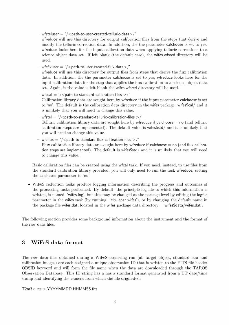
– wfsteluser = ‘/<path-to-user-created-telluric-data>/’wfreduce will use this directory for output calibration files from the steps that derive andmodify the telluric correction data. In addition, the the parameter calchoose is set to yes,wfreduce looks here for the input calibration data when applying telluric corrections to ascience object data set. If left blank (the default case), the wifes.wfsred directory will beused.

– wfsflxuser = ‘/<path-to-user-created-flux-data>/’wfreduce will use this directory for output files from steps that derive the flux calibrationdata. In addition, the the parameter calchoose is set to yes, wfreduce looks here for theinput calibration data for the step that applies the flux calibration to a science object dataset. Again, it the value is left blank the wifes.wfsred directory will be used.

– wfscal = ‘/<path-to-standard-calibration-files >/’Calibration library data are sought here by wfreduce if the input parameter calchoose is setto ‘no’. The default is the calibration data directory in the wifes package: wifes$cal/ and itis unlikely that you will need to change this value.

– wfstel = ‘/<path-to-standard-telluric-calibration-files >/’Telluric calibration library data are sought here by wfreduce if calchoose = no (and telluriccalibration steps are implemented). The default value is wifes$std/ and it is unlikely thatyou will need to change this value.

– wfsflux = ‘/<path-to-standard-flux-calibration-files >/’Flux calibration library data are sought here by wfreduce if calchoose = no (and flux calibra-tion steps are implemented). The default is wifes$std/ and it is unlikely that you will needto change this value.

Basic calibration files can be created using the wfcal task. If you need, instead, to use files fromthe standard calibration library provided, you will only need to run the task wfreduce, settingthe calchoose parameter to ‘no’.

• WiFeS reduction tasks produce logging information describing the progress and outcomes ofthe processing tasks performed. By default, the principle log file to which this information iswritten, is named ‘wifes.log’, but this may be changed at the package level by editing the logfileparameter in the wifes task (by running ‘cl> epar wifes’), or by changing the default name inthe package file wifes.dat, located in the wifes package data directory: ‘wifes$data/wifes.dat’.

The following section provides some background information about the instrument and the format ofthe raw data files.

3 WiFeS data format

The raw data files obtained during a WiFeS observing run (all target object, standard star andcalibration images) are each assigned a unique observation ID that is written to the FITS file headerOBSID keyword and will form the file name when the data are downloaded through the TAROSObservation Database. This ID string has a has a standard format generated from a UT date/timestamp and identifying the camera from which the file originated:

T2m3< xx >.YYYYMMDD.HHMMSS.fits

3

where xx are characters that represent the camera of origin: ‘wr’ for the WiFeS red camera, ‘wb’ forthe WiFeS blue camera and ‘Ap’ for the field viewing camera; and YYYYMMDD is the UT date andHHMMSS the UT time associated with the file’s creation.

The layout of a raw WiFeS image is shown in Figure 1. There are four detector quadrants (A, B, C,D) that are each read out through a separate amplifier with overscan columns at the left of quadrantsA and D and to the right of B and C. The horizontal axis is the dispersion axis, and the verticalaxis contains the 2D sky plane in 25 horizontal slices (perpendicular to the slices on the sky) eachapproximately 80 pixels in height (the direction along the slices sky). There are 25 ‘primary’ slicepositions (Figure 1, left), and these are interleaved by the 25 ’secondary’ slice positions to which thecharge is shuffled in ‘nod-and-shuffle’ observing mode (the final location of the ’secondary’, or sky,image). The data reduction scripts reconstruct the raw, dispersed data into a data cube consisting ofa set of wavelength calibrated image planes.

1:2069

1:2

04

8

(A)

4:21

22:2069

1:2048

2049:20661:2

04

8

1:3

2070:4117

4118:4135

4136:4138

2067:2069

20

49

:40

96

22:2069

4:21

1:3

2069:4138

4:2069 2070:4135

4:2069 1:2066

1:2069 1:2069

(1,1)

(4138, 4096)

1

(B)

2

(D)

4

(C)

3

6

The row of slit images is formed half-way between theslicer and the collimator. In this configuration, the raybundle associated with each slitlet strikes the collimatorat normal incidence and the returning collimated beamsfrom all slitlets form a common pupil at the plane ofthe grating which is co-planar with the image slicer. Byminimizing off-axis angles, this ‘concentric’ approachensures excellent and uniform image quality across thefield.

The slicer and stacker presents to the WiFeS spec-trograph what is in effect a very long-slit format withseparated segments corresponding to each slice. Indeed,the effective slit is so long that field angle effects on thegrating are appreciable. The fan angle on the imageslicer is chosen so that the slitlet image at the stackeris separated by just over its own length from its neigh-bours. Together these provide an image format on thedetector shown in Figure 3.

This format may look wasteful from the viewpointof efficient use of the detector real estate, but it doesoffer a notable advantage for the detection of very faintobjects, since it allows for what we have termed “in-terleaved nod-and-shuffle" on the CCD. The techniqueof nod-and-shuffle is well-developed Cuillandre (1994);Tinney (2000); Glazebrook (2001), and provides for ex-cellent sky-subtraction because, for any spatial or spec-tral position, both object and sky are observed virtuallyat the same time, for the same time, and on the samepixel. This allows for

√N statistics in the removal of

unwanted sky signal from the object signal.The implementation of nod-and-shuffle in WiFeS is

to expose for a short period of time, typically 30s. Theshutters are closed, and the charge on the CCDs trans-ferred in the x−direction by the width of each slitlet(∆x pixels) to move the object signals into the inter-slit space. The telescope is nodded to the reference skyposition and a sub-exposure of the same length is taken.The shutter is again closed, charge shuffled back to itsoriginal coordinate, and the telescope returned to thetarget position. The whole process is then repeated asmany times as necessary. Sky subtraction is achievedby subtracting each part of object signal from the sig-nal located ∆x pixels from the object signal. An on-frame bias signal is provided along the chip edge wherethe charge shuffling causes charge to be repeatedly lost‘overboard’.

Since there remains a risk that the de-rotator axisand the telescope field rotation axis are not preciselyaligned, both offset guiding and through entrance slotacquisition cameras are provided (but not shown in Fig-ure 1. The second camera is fed by a flip mirror im-mediately in front of, and mechanically coupled to, theimage slicer. This enables the observer to re-centre the

Fig. 2.— The WiFeS image slicer in its final fannedconfiguration mounted in its mandril which also servesas a mounting block for the slicer in the instrument.

Fig. 3.— The image format on the detector for theB7000 grating. The long wavelength part of the spec-trum is on the left. Other gratings give very similar for-mats, but the spectral dispersion direction is reversed inthe red arm. Note the spaces between adjacent spectraallow ‘nod-and-shuffle’ sky subtraction to be achieved.The sky spectra are accumulated in these spaces, andsky subtraction is acheived by shifting the image withrespect to itself by 80 pixels, and then subtracting itfrom the unshifted image.

Overs

can

extra columns

Overs

can

Overs

can

Overs

can

extra columns

Primary / 'object' slice positions

Secondary / shuffled sky

slice positions

Figure 1. Left: layout of amplifier regions in the raw images. Grey arrows show pixel dimensions / rangeswithin the individual (‘local’) amplifier coordinate systems, and the black arrows and labels refer to ‘global’positions and dimensions in the raw image, within the whole array of amplifier regions. Right: an exampleraw (blue camera) image showing the positions of the primary, or object, slit positions on the detectorilluminated by an arc calibration lamp and the secondary positions that will be filled by sky observationsor nodded object exposures in nod-and-shuffle mode.

WiFeS raw images are single-extension FITS files, about 32 MB in size (pixel values stored as 8 bitunsigned short integers). The data are converted to multi-extension FITS (MEF) files with two fileextensions by the WiFeS data reduction script wftable. Header information is written to the primaryheader unit (PHU) in extension [0], and image data is placed in extension [1]. The WiFeS pipelinetasks add header information during processing to document important parameter values and the datareduction steps that have been completed. The image data are converted to ’real’ data type early inprocessing, so the file size of the original data increases by a factor of four even before any additionalinformation is added.

Pre-processing with package task wfprepare trims the overscan regions from the images, after optionallyusing it to subtract an averaged bias signal, and generates and adds variance [VAR] and data quality

4

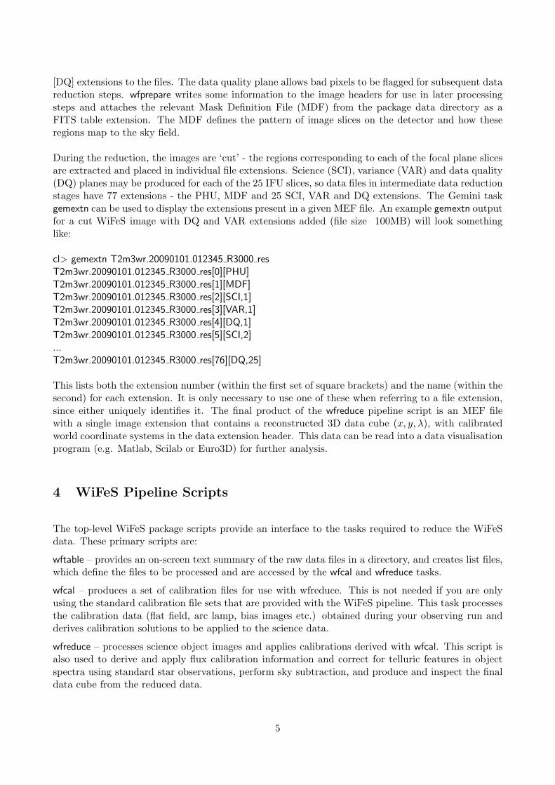
[DQ] extensions to the files. The data quality plane allows bad pixels to be flagged for subsequent datareduction steps. wfprepare writes some information to the image headers for use in later processingsteps and attaches the relevant Mask Definition File (MDF) from the package data directory as aFITS table extension. The MDF defines the pattern of image slices on the detector and how theseregions map to the sky field.

During the reduction, the images are ‘cut’ - the regions corresponding to each of the focal plane slicesare extracted and placed in individual file extensions. Science (SCI), variance (VAR) and data quality(DQ) planes may be produced for each of the 25 IFU slices, so data files in intermediate data reductionstages have 77 extensions - the PHU, MDF and 25 SCI, VAR and DQ extensions. The Gemini taskgemextn can be used to display the extensions present in a given MEF file. An example gemextn outputfor a cut WiFeS image with DQ and VAR extensions added (file size 100MB) will look somethinglike:

cl> gemextn T2m3wr.20090101.012345 R3000 resT2m3wr.20090101.012345 R3000 res[0][PHU]T2m3wr.20090101.012345 R3000 res[1][MDF]T2m3wr.20090101.012345 R3000 res[2][SCI,1]T2m3wr.20090101.012345 R3000 res[3][VAR,1]T2m3wr.20090101.012345 R3000 res[4][DQ,1]T2m3wr.20090101.012345 R3000 res[5][SCI,2]...T2m3wr.20090101.012345 R3000 res[76][DQ,25]

This lists both the extension number (within the first set of square brackets) and the name (within thesecond) for each extension. It is only necessary to use one of these when referring to a file extension,since either uniquely identifies it. The final product of the wfreduce pipeline script is an MEF filewith a single image extension that contains a reconstructed 3D data cube (x, y, λ), with calibratedworld coordinate systems in the data extension header. This data can be read into a data visualisationprogram (e.g. Matlab, Scilab or Euro3D) for further analysis.

4 WiFeS Pipeline Scripts

The top-level WiFeS package scripts provide an interface to the tasks required to reduce the WiFeSdata. These primary scripts are:

wftable – provides an on-screen text summary of the raw data files in a directory, and creates list files,which define the files to be processed and are accessed by the wfcal and wfreduce tasks.

wfcal – produces a set of calibration files for use with wfreduce. This is not needed if you are onlyusing the standard calibration file sets that are provided with the WiFeS pipeline. This task processesthe calibration data (flat field, arc lamp, bias images etc.) obtained during your observing run andderives calibration solutions to be applied to the science data.

wfreduce – processes science object images and applies calibrations derived with wfcal. This script isalso used to derive and apply flux calibration information and correct for telluric features in objectspectra using standard star observations, perform sky subtraction, and produce and inspect the finaldata cube from the reduced data.

5

These tasks are described in more detail in the following sections.

There is also a simple task available to generate a ‘log’ of the properties of a set of WiFeS image files.The task wflog extracts and lists values of selected keywords from the image headers. If an output filename is be provided in the logfile input parameter, the table of image header values will be printed to atext file of that name. This file will be created if it does not already exist, or the data will be appendedto an existing file. If the field is left blank, or the value ‘stdout’ is provided, the log information willbe printed to the screen in the command window. The filestr parameter is used to tell the routinewhich files should be included in the log and is a template of the sort that can be input to the IRAFsystem.files task to be expanded into a list of file names. For example, the default is to include allfiles in the current directory with the template ‘*.fits’, and providing the string ‘T2m3wr*.04*fits’ willcause observation data for only the red camera images in the current directory observed between 04:00and 05:00 UT (for raw files with the standard filenames written by the TAROS software) to be listed.

The remaining parameters correspond to a set of keywords from WiFeS image headers. Assigning anon-zero integer to those required in the log file indicates the column in which that keyword valueshould appear in the log. The first column will contain the image file name and each of the parametersspecified will be in the following columns, ordered by the input value given (and then alphabeticallyby the parameter name if the same integer is assigned to multiple parameters). The final two pairsof input parameters allow custom header keywords that are not included in the parameter list to beselected for inclusion in the log file. A keyword as it appears in the headers is required as the key1and/or key2 parameter values, and the column index is specified in the col1 and/or col2 parameters(which must be changed to values greater than zero for the parameter to be written to the log).

4.1 WFTABLE: Reformat, summarise and sort image files

USAGE

cl> wftablecl> wftable image=<image file>cl> wftable grating=<grating name>cl> wftable grating=<grating name> dichroic=<dichroic name>

PARAMETERS

grating = <grating name> : WiFeS grating (U7000, B7000, R7000, I7000, B3000 or R3000) A gratingidentifier is given here to define the set of files to be described and included in list files (name may begiven as upper or lower case).dichroic = <dichroic name> : WiFeS dichroic (RT480, RT560, RT615)A dichroic (beam splitter) identifier (may be upper or lower case) can also be provided to constrainthe set of files to be described and included in the lists. If this parameter is not specified when agrating value is, the ‘standard’ combination for the grating will be assumed.image = <image file> : Image to be processed (“*” for all)

If an image file name is provided as the value of this parameter, only this specified image will beprocessed with wftable. By default (if image=“*”) all images found in the current directory will beaccessed by the task.

DESCRIPTION AND INSTRUCTIONS

6

wftable tabulates key data from raw image file headers, reformats raw data into multi-extension FITS(MEF) files and creates reduction file lists to which wfcal and wfreduce refer. This task needs to berun in two steps: first without the grating and dichroic parameter values set to convert the data toMEF files and produce a summary of all the raw data, and second with the grating and optionallythe dichroic value set to produce the list files.

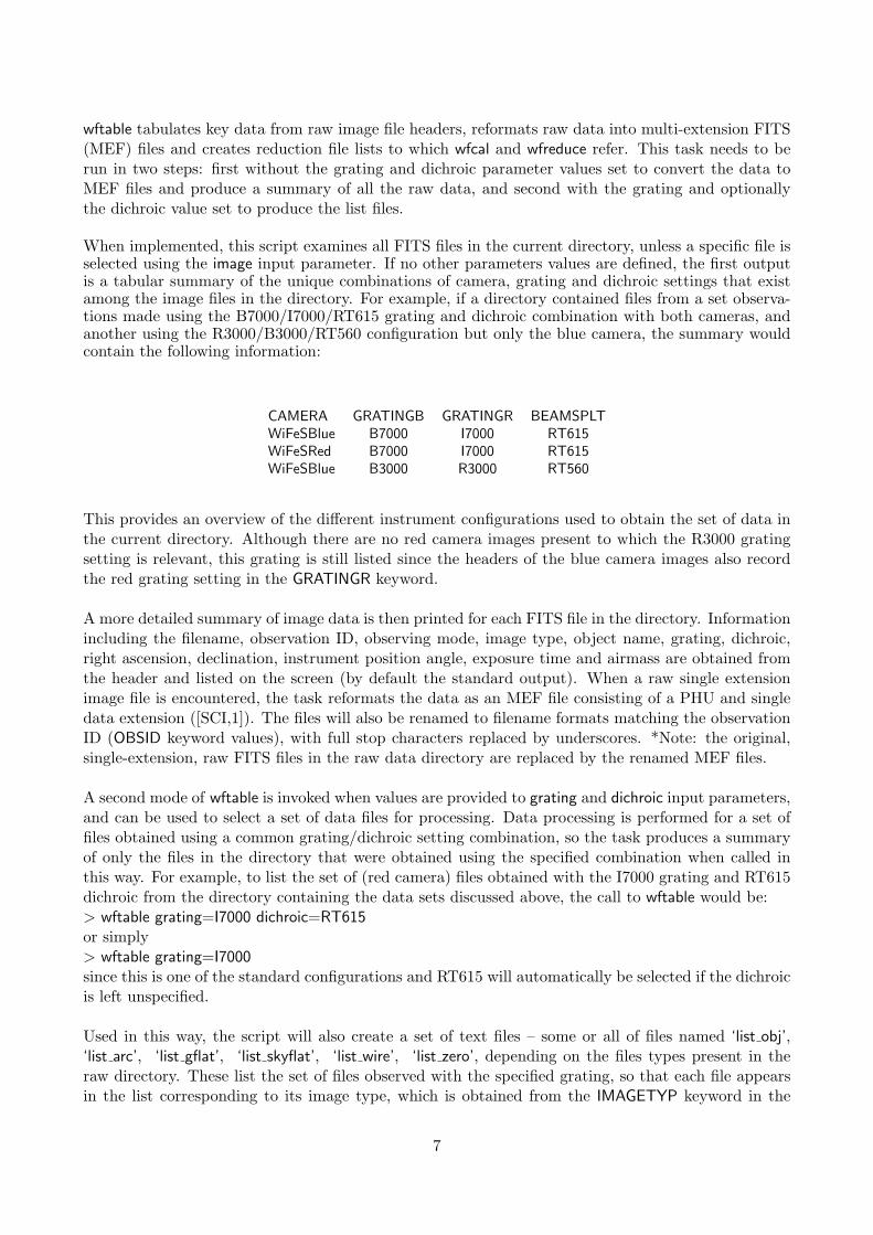
When implemented, this script examines all FITS files in the current directory, unless a specific file isselected using the image input parameter. If no other parameters values are defined, the first outputis a tabular summary of the unique combinations of camera, grating and dichroic settings that existamong the image files in the directory. For example, if a directory contained files from a set observa-tions made using the B7000/I7000/RT615 grating and dichroic combination with both cameras, andanother using the R3000/B3000/RT560 configuration but only the blue camera, the summary wouldcontain the following information:

CAMERA GRATINGB GRATINGR BEAMSPLTWiFeSBlue B7000 I7000 RT615WiFeSRed B7000 I7000 RT615WiFeSBlue B3000 R3000 RT560

This provides an overview of the different instrument configurations used to obtain the set of data inthe current directory. Although there are no red camera images present to which the R3000 gratingsetting is relevant, this grating is still listed since the headers of the blue camera images also recordthe red grating setting in the GRATINGR keyword.

A more detailed summary of image data is then printed for each FITS file in the directory. Informationincluding the filename, observation ID, observing mode, image type, object name, grating, dichroic,right ascension, declination, instrument position angle, exposure time and airmass are obtained fromthe header and listed on the screen (by default the standard output). When a raw single extensionimage file is encountered, the task reformats the data as an MEF file consisting of a PHU and singledata extension ([SCI,1]). The files will also be renamed to filename formats matching the observationID (OBSID keyword values), with full stop characters replaced by underscores. *Note: the original,single-extension, raw FITS files in the raw data directory are replaced by the renamed MEF files.

A second mode of wftable is invoked when values are provided to grating and dichroic input parameters,and can be used to select a set of data files for processing. Data processing is performed for a set offiles obtained using a common grating/dichroic setting combination, so the task produces a summaryof only the files in the directory that were obtained using the specified combination when called inthis way. For example, to list the set of (red camera) files obtained with the I7000 grating and RT615dichroic from the directory containing the data sets discussed above, the call to wftable would be:> wftable grating=I7000 dichroic=RT615or simply> wftable grating=I7000since this is one of the standard configurations and RT615 will automatically be selected if the dichroicis left unspecified.

Used in this way, the script will also create a set of text files – some or all of files named ‘list obj’,‘list arc’, ‘list gflat’, ‘list skyflat’, ‘list wire’, ‘list zero’, depending on the files types present in theraw directory. These list the set of files observed with the specified grating, so that each file appearsin the list corresponding to its image type, which is obtained from the IMAGETYP keyword in the

7

header. The expected set of keyword values and the list files to which images with these values willbe assigned are summarised in Table 1.

Table 1. Image type keyword values and the list files in which an image will be included if it has thatIMAGETYP value in the header.

IMAGETYP List file Image typevalue

flat list gflat usually calibration lamp flat field framesskyflat list skyflat twilight / sky flat field imageswire list wire flat field images with coronograph/‘wire’ aperturearc list arc arc lamp imageszero list zero bias frames

The wfcal and wfreduce routines use these list files to determine the input files for the various processingsteps. The files can, of course, be created or edited by hand to add or remove the files to be includedin the processing. When the data reduction for files in the identified data set has been completed, youcan run wftable with another combination of grating and dichroic values, to re-write the list files andset up to reduce the next set of data.

4.2 WFCAL: Reducing calibration data

USAGE

To edit the input parameters that control the script functions:cl> epar wfcal

To run the script:cl> wfcal

PARAMETERS

The following parameters determine which steps in the data reduction are carried out:dounlearn = yes : Unlearn all Gemini parameter sets?dowfprepare = yes : Do wfprepare steps?dooverscanbias = no : Use overscan regions for bias subtraction?dorefflat = yes : Create reference flat frame?dozero = yes : Create median-averaged bias frame?dogflat = yes : Create flat field frame?dosflat = yes : Process sky flat field frames and correct flat field?doarc = yes : Create wavelength scale calibration?dowire = yes : Create spatial scale calibration?

The following parameters allow several input and output directories and file names to be redefined, ifdesired:outdir = “ ” : Output directory for calibration filesoutname = “ ” : Output file root (no spaces, filename format)reference = “ ” : Name of slitlet geometry reference filebiasframe = “ ” : Existing bias frame to be usedinter flat = yes : Run flat field steps interactively (dogflat, dosflat)?sflat dir = “ ” : Directory from which to copy reduced sky flat imageslit sample = “ ”, Sample region for flat field fit to profile along slits?

8

arcidx = “ ” : Index to identify arc framedatabase = ‘database’ : Name of directory for database fileskeepfiles = no : Keep intermediate data reduction files?

DESCRIPTION AND PROCEDURES

wfcal is used to process WiFeS calibration data (including flat field, arc lamp, bias and corono-graphic/‘wire’ flat field images). The solutions and data that are produced by this task can then beapplied in the reduction of science observations with wfreduce. The input data is supplied to wfcalthrough the wifes.wfsraw directory definition and a set of list files located there (which can be generatedby wftable).

The series of ‘do<step>’ input parameters essentially describe the steps that can be implemented inwfcal and most correspond to processing the different types of calibration data. Though these stepsto do not all have to be implemented in series, there are some dependencies among them.

The dowfprepare parameter determines whether wfprepare is called at the beginning of each processingstage. The images need to be ‘prepared’ before further processing can be undertaken, but onceprepared images have been produced (these have the same file name as the raw image, but with an ‘n’prefix), this step can be skipped to save time if processing steps are being repeated. wfprepare trimsoff the overscan columns (after optionally using them to average and subtract a bias level from theimage - see the description of the dozero step below), calculates and attaches a variance image as anew extension and forms a data quality extension in which bad pixels and pixel values exceeding 95%of the saturation limit are flagged. The appropriate MDF is located and also attached as an imageextension and the required offsets of the MDF obtained (calculated by cross-correlation if the imageis a reference flat or obtained from the reference image if it is not) and written to the image header.

At several points, the script prompts for input from the user and runs interactive tasks in the IRAFgraphics terminal. These sequences are discussed further in the descriptions of the relevant processingsteps below.

Various intermediate and temporary files are created as part of the calibration process. These aredeleted by the automatic ‘cleanup’ at the end of the task (which is invoked if the script safely haltsexecution after a known error occurs or successfully finishes), unless the keepfiles parameter to ‘yes’.This could rapidly fill up your available disk space, so it may be best to set this parameter to yes onlyif you are encountering problems.

The individual stages of the wfcal script is described in some detail below.

Prepare IRAF environment:The script prepares to process the calibration files by checking that the various input and outputdirectories can be accessed (some required directories may be created), opening the log file, obtainingnecessary WiFeS header keywords using the wfheaders task, and setting file and other variable values.The current directory is changed to the calibration directory where output files will be written. If anaccessible directory is provided in the input parameter outdir, this will be used for output; otherwise,output files will be placed in the location defined by the package parameter wifes.wfscalu. If this valueis an empty string (the default), the directory ‘caluser’, inside the ‘wifes.wfsred’ directory will be used(it will be created if it does not already exist).

A database directory, by default named ‘database’, will be created or accessed in the output directory

9

to store calibration solution files produced by the identify routines in deriving the wavelength andspatial calibrations. The directory name can be altered by changing the default in the database inputparameter, but this should not generally be necessary and is not recommended.

The names of output files are constructed from the calibration type and a root string that is appended.By default the file name root is formed from the names of the grating and dichroic used for the obser-vations: that is, it has the form: ‘[grating name] [dichroic name]’. This can be changed by providingan alternative string to the outname parameter, however.

Prepare reference flat and determine shifts (dorefflat):A single image is used to register the geometry of the illumination pattern on the detector. wfpreparecross-correlates the illumination profile in a selected flat field (or similar) frame with the appropriatemask-definition file (MDF) that defines the expected slitlet geometry, to determine any shifts thatneed to be applied when the MDF is used to extract the individual slice regions. This step requiresthe user to interactively fit a profile to the correlation function, using the Gaussian fit function of theinteractive IRAF splot environment, to locate the peak (use the ‘k’ key to mark the left and rightedges of the wings of the function).If the input parameter reference is left empty, wfcal will attempt to use a flat field images as thereference frame (the last image in the ‘list gflat’ or ‘list sflat’ list, in that order). The prepared referenceimage file has the name of the input image with an ‘s’ prefix. A copy is also output with the ‘standard’filename: ‘refflat <outname>.fits’ or ‘refflat <grating name> <dicroic name>.fits’.If a reference flat exists and this step is not implemented (dorefflat=no), the task looks for an existinggeometry reference frame to use for the other images in a similar way to choosing a frame to reduceas above. A raw image filename can be provided in the reference parameter and wfcal will check if aversion of this file that has been prepared as a reference flat exists in the output directory (given inoutdir or wifes.wfscalu); i.e. there should be a file ‘s<reference>’ in this directory. If this file can’t befound, a check is made for a reference flat formed from either the last image in the list of lamp flatfield images or the sky flat field images (as would be used by default when creating a reference flat).If neither reference flat can be found, wfcal exits with an error.

Reduce and combine the zero or bias frames (dozero):If dozero is ‘yes’ each bias image in the ‘list zero’ file is prepared and combined into a single biasframe using the median in each pixel. The output filename has the format ‘zero <camera>.fits’. Thisframe will be used in subsequent steps to subtract the bias signal from each of the calibration images,unless the parameter dooverscanbias is ‘yes’, in which case the detector overscan regions will always beaveraged and used for bias subtraction during the wfprepare in each step. If dozero and dooverscanbiasare not set, the script runs through a series of options to determine whether there is a bias image isavailable for bias subtraction. First, the biasframe input parameter is checked for an accessible biasimage file name, which is used if found. If this parameter is empty the script checks if a previouslygenerated bias with the standard name exists in the output directory. If not, an appropriately-namedbias image is sought in the calibration library directory (wifes.wfscal). If this is not found, a promptappears in the terminal notifying the user that a bias frame couldn’t be found and asking whether touse the overscan regions for bias subtraction. If the response given is not ‘yes’, the task gives up indespair and exits.

Reduce and combine the flat field images (dogflat):The pipeline is set up to form a ‘master’ flat field image with the dogflat step (most likely fromcalibration lamp or ‘ground’ flat field images: quartz-iodide lamps are available in the DBS calibrationsystem), and then to correct this flat field image for uneven illumination along the slitlets using a ‘sky’(or twilight) flat field image in the dosflat step. If you are using only sky flats for flat fielding (as

10

must be done when observing with the U7000 grating, as neither the QI or dome flat lamps producesufficient UV flux), these can be reduced using the dogflat step: for example, copy the wftable sky flatlist to the ground flat list: > cp list sflat list gflat and run wfcal with dogflat=yes (and dosflat=no).

If dogflat is set, the flat field images listed in the file ‘list gflat’ are prepared, combined and reduced. Thewfflat task is used to fit a polynomial to the illumination in the dispersion direction – if the parameterinter flat is ‘yes’, this fit is displayed and can be altered interactively – and produce a normalised flatfield image in each slice extension. If dosflat is ‘no’, the flat field image output by wfflat is assumed tobe the final flat field frame and wfslitfunction is used to restore the relative illumination between theslices in different image extensions (wfflat normalises each extension independently of one another).

Reduce the sky flats (dosflat):If dosflat is on, it is assumed that a flat field image has already been produced with dogflat. When thisstep is also set , the images listed in the ‘list sflat’ file (twilight sky flats) are prepared, combined andreduced. This combined ‘sky’ flat is then used by the wfslitfunction task to correct the illuminationprofile in the spatial direction along the slit in the calibration lamp / or ‘master’ flat that was createdin the dogflat step that preceded.

If your sky flats were obtained on a different night and/or were most appropriately prepared andreduced with another set of calibrations (e.g. from that night), you can provide the output calibra-tion directory for that previous set of (reduced) calibrations in the wfcal input parameter sflat dir.The pre-prepared and combined sky flat field frame found in that directory (with default name‘rsflat <grating name> <dicroic name>.fits’ or custom name ‘rsflat <outname>.fits’) will then be usedto correct the lamp flat. It is important to make sure that this parameter is empty if you are reducingraw sky flats with the current set of calibrations.

If the interactive flag in the input parameters, inter flat, is set to ‘yes’ the profile fitting can be inspectedand changed interactively. The task divides the spectral axis into ten bins along the dispersion directionand derives a fit to the illumination over the direction along the slice length in each of these bins foreach slice. This means that potentially you can look at 250 profile fits, which would be just a littletedious. However, the principal aim is to ensure that the sample region (along the slit) over which thefit is made is appropriate and excludes sufficient portions at either end of the slit where the sensitivityfalls off rapidly. You may want to inspect the results for the first couple of slices, several in the middle(slice 13) and the last few, checking that the region is appropriate (and the profile is well fit) acrossthe whole image. If the default sample region needs to be changed, re-run the dogflat and dosflatsteps of wfcal after providing a new sample region in the slit sample parameter (a string of the form‘[pixel1]:[pixel2]’). You can set the inter flat parameter to ‘no’ to turn off the interactive mode for thesesteps.

Reduce arc lamp images and determine wavelength solution (doarc):Arc lamp images listed in ‘list arc’ are prepared, combine and reduced if doarc is ‘yes’. There aretwo options for running the arc line identification procedures in wfcal. The script stops and asks theuser whether to use a ‘reference’ wavelength solution to assist in the arc line identification or whetherto run the autoidentify routine and have the opportunity to inspect, edit or manually match the lineidentifications and dispersion solution. If the user responds with ‘yes’, a previous solution for the givengrating and dichroic combination and the arc lamp spectrum is sought from the calibration library.This is used as the starting point for the wavelength solution, allowing the autoidentify routine to beskipped. The reidentify task takes this previous result for the first row considered in each slice andtraces it through the rest of the image to derive the complete calibration. Unfortunately, there is not yeta set of reference solutions for all of the arc lamp and grating/dichroic combinations in the calibration

11

library, so if the one you require does not exist, this option will not work. There are currently referencesolutions for the NeAr lamp with each of the standard grating/dichroic combinations, and solutionsfor the CuAr lamp with the B3000/R3000/RT560 and B7000/I7000/RT615 configurations.

If the reference solution method is not selected (answering ‘no’ to the first prompt - the default),autoidentify attempts to match the detected lamp lines with the provided line list (with varying degreesof success for the different gratings). Labelled arc spectra are provided in the calibration library forreference and more details about the arc line matching is provided in the task help files.

It is likely that a set of calibrations includes multiple arc frames obtained at different times throughoutthe night. The arcidx input parameter to wfcal can be used to distinguish between these. The valueprovided can consist of any string, which will be appended to the processed arc file name and associatedcalibration solution files in the database directory. So, for example, you can sequentially change thearc file names in the list arc file and process each by running wfcal with just doprepare and doarc turnedon, changing arcidx for each one: e.g. use ‘1’, ‘2’, ‘3’, etc. for arcidx. When reducing a science objectobservation with wfreduce, the same identifying string can be input to its arcidx parameter to indicatewhich wavelength solution to apply.

Align the spatial scales along each slit (dowire):Flat field images obtained with the coronographic aperture mask (or ‘wire’) in the field are used in thisstep to align the slitlets. The wire extends across the WiFeS field, so it is imaged at a fixed positionin all slitlets, and this forms the reference ‘zero’ point for the spatial scale in this direction.If the dowire step is selected, the wire images are prepared, combined and reduced, and a check is madeto ensure there is a corresponding flat field image available (either from the current output directoryor the default calibration library). Two new wire images are formed by shifting the combined frame byset offsets (+10 and -15 pixels) and an image containing three positive traces is produced by combiningthese and subtracting from a flat frame. The IRAF identify tasks are then employed by wfsdist tolocate and obtain a coordinate scale using these peaks in the column profiles and to trace this alongthe image rows. The solution data are output to the database directory.Before this process begins, the script prompts the user about whether to run the trace detectionautomatically (without the opportunity for user input) or to run the identification ‘manually’ so thatthe results can be confirmed and modified if required. If ‘yes’, a profile of each slice will be displayedin turn, and typing an ‘e’ prompts the task to attempt to locate the peaks of the wire traces. This isusually successful - all three are marked and typing a full stop with the cursor positioned over eachshows the position that it corresponds to (the expected positions are printed in the command window).If a line is missed, it can be marked with an ‘m’ and the correct value entered. In the non-interactivemode, the task simply performs these steps automatically and displays the result of the each matchto the graphics window. You can check that all traces are successfully found, but not alter the result.If any are missed you will have to re-run the dowire step again interactively.

4.3 WFREDUCE: Reducing and calibrating science data

USAGE

To edit the input parameters and control the script functions:cl> epar wfreduce

To run the script:cl> wfreduce

12

PARAMETERS

The following parameters select which steps in the data reduction are carried out:quicklook = no : Run a quicklook reduction to view data?calchoose = yes : Use your own calibration data (from wifes.wfscalu)?telchoose = yes : Use your own telluric/flux data (from wifes.wfstelu)?dounlearn = yes : Unlearn parameter sets?dowfprepare = yes : Do wfprepare steps?docombine = yes : Combine multiple object frames?dozero = yes : Subtract averaged zero from combined object and sky frames?dooverscanbias = no : Use overscan region average to subtract bias level?dosubshuffled = no : Subtract shuffled sky from object data?doskyframes = no : Reduce and subtract sky images (listed in list sky)?doskycal = no : Derive wavelength calibration from separate sky frame?doreduce = yes : Reduce combined object image?dofixbad = no : Fix bad pixels flagged in DQ array?dofitcoords = yes : Fit coordinates to correct for spectral and spatial distortion?dotransform = yes : Produce transformed 3D data cube using nftransform?dotrimcube = yes : Trim low-signal border regions from cube?dosubsky = no : Subtract averaged sky spectrum from within cube?dotelextract = no : Extract a telluric star spectrum?dofixtell = no : Fix stellar absorption in telluric spectrum?dotelcorrect = no : Apply telluric correction to data cube?dofluxextract = no : Extract a flux standard spectrum?dofluxcalibrate = no : Apply flux calibration to data cube?dodar = no : Correct data cube for differential atmospheric refraction?doscience = yes : Extract a science object spectrum and projected image?dointcube = no : Interpolate to form cube with 0.5′ square pixels?dosimcube = no : Output a simple FITS cube for NF3D?dothroughput = no : Plot throughput over band?

The remaining parameters provide information used by various steps in the processing:keepfiles = no : Keep intermediate data reduction files?calname : Calibration file name baseskyfactor = 1.000 : Factor by which to scale sky signalreftrans = “ ” : File defining coordinate transformation to match

The next six parameters are used to extract an integrated spectrum and projected image from thereduced data cube:sciaper = 5.0 : Science object aperture diameter (arc sec.)emission = yes : Spectral feature is an emission line?waverest = 0.65628 : Feature rest wavelength (microns)redshift = 0.05 : Object redshiftvstart = -200.0 : Start velocity range (km/s)vstop = 200.0 : Stop velocity range (km/s)

arcidx = “ ” : Index of arc frame for wavelength calibrationtelluric = “ ” : Filename of spectrum extracted for telluric correctiontelaper = 5.0 : Telluric aperture diameter (arcsec)tellfile = ‘wifes$data/smooth star redlines.dat’ : Data file providing stellar absorption feature datafluxstd = “ ” : Filename of spectrum extracted for flux calibrationfluxaper = 15.0 : Flux standard aperture diameter (arc sec.)

13

fluxstar = “ ” : Flux standard star name skyfile = “ ” : Sky line list file name

DESCRIPTION AND PROCEDURES

Target object data files are processed with wfreduce. This routine applies the calibration solutionsderived using wfcal to science and standard star frames, performs sky-subtraction, constructs the 3Ddatacube from the processed images, and derives and applies corrections for telluric features in spectraand for flux calibration. wfreduce identifies the input image files to be processed by accessing text listfiles, such as those that can be produced with wftable, in the raw data directory (wifes.wfsraw).

During the processing, wfreduce displays processed files at intermediate stages in the image viewer(e.g. DS9) and prints information and progress information to the terminal window and to a log file.In some case it is possible to activate more extensive debugging information by editing the parametersof individual tasks called by the wfreduce script. Several of the reduction steps are interactive andrequire user input in the IRAF command line terminal, in the graphics terminal or in the image frame.These are discussed further below in the descriptions of each stage of processing.

The task produces new files during some steps in the reduction, generally when the data format ischanged, however many steps will work on and alter the output file, so that the process can be startedfrom intermediate stages. If a particular step needs to be repeated, it may be necessary to also repeatpreceding steps to recreate the file in the current format and avoid simply applying the procedure tothe output file multiple times.

Various intermediate and temporary files are created during the data processing. These are deletedby the automatic ‘cleanup’ at the end of the task (which is invoked if the script safely halts executionafter a known error occurs or successfully finishes), unless the keepfiles parameter is set to ‘yes’. Thiswill rapidly generate a number of cryptically-named temporary files, so it may be best to set thisparameter only if you are encountering problems and searching for results at a particular intermediatepoint.

A number of output files are produced by the processing steps. Many of these files have file namesconstructed from an OBSID (from the last raw image file name in the object list), of the form:obsid = T2m3w[r/b] [ddmmyy] [hhmmss], an ID string identifying the grating and dichroic used forthe observation, of the form: idstr = [grating] [dichroic], and a suffix that depends on the stage ofprocessing at which it was produced.

There is a ‘quick-look’ option in wfreduce that can be used to construct a data cube from a rawframe in the minimum time (for example, to examine data at the telescope while observing).1 It isinvoked by setting the quicklook input parameter to ‘yes’, which will automatically select the set ofdata processing steps to be applied (when the script is run). Calibration data is obtained from the setof ‘standard’ calibrations included in the wifes package (by default found in the wifes$cal/ directory),so approximate solutions are applied to the data.A single image is reduced in quick-look mode. The input file is still obtained from a ‘list obj’ text filein the raw directory, but only the last frame in the file will be processed if more than one image islisted. A projected image and integrated spectrum will be extracted from the cube and displayed. Theimage is saved as file ‘quickim.fits’ in the reduction output directory (wifes.wfsred), and is formed usingthe emission, waverest, redshift, vstart and vstop parameters (set emission=no for an image formed bycollapsing the whole cube along the dispersion axis; see descriptions below). After the cube is formed,

1On MSO machines ‘moron’ and ‘maggot’ this takes about 2 minutes.

14

the projected image is displayed in the image viewer and the user is prompted to mark the centre ofthe aperture from which an integrated spectrum will be formed (the aperture diameter is specifiedwith the sciaper parameter). The integrated spectrum is interactively plotted using the IRAF splottask and when this is quit (type ‘q’), the projected image is redisplayed in the image window. Thisoutput image file is resampled to a 50×76 pixel grid, so that the pixels are approximately square(∼ 0.5′ × 0.5′).

A basic wrapper task for the quick-look mode is available in the package: wfquick. The input to thistask is a raw image file name, and optionally the file location on a remote computer, and the taskconstructs the image list with wftable, and sets up and runs wfreduce in the quick-look mode. See thehelp file in the package for more detail on the use of this task (i.e. type > help wfquick after loadingwifes).

The key stages in the processing implemented with wfreduce are discussed below.

Set up the IRAF environmentwfreduce prepares to process the object files by selecting input and output directories based on thewifes parameters and the calchoose and telchoose parameter values, and checking that the requireddirectories can be accessed (some directories may be created). The log file is opened, the necessaryWiFeS header keywords are imported using the wfheaders task, various file and other variable values areset and the calibration data is copied from the wifes.wfscaluser (if calchoose=yes) or the wifes.wfscal (ifcalchoose=no) directory to the ‘database/’ directory in the output location (wifes.wfsred). Calibrationfiles with the default name formats are sought, unless a file name base is provided in the calnameparameter. This is useful if a non-default name was assigned to the calibration files through thewfcal.outname when they were created with wfcal (the default naming system uses a base stringcomprised of the grating and dichroic identifiers: [grating] [dichroic].fits).The current directory is changed to the reduction directory, wifes.wfsred, where output files will bewritten.If dounlearn is selected, the input parameters for tasks in the packages used by the wifes scripts (gemini,gemtools, gnirs, nifs) will be reset using the IRAF unlearn command.If the quick-look mode is selected, the input do[step] parameter values are changed as necessary to turnon the steps and parameters needed to use the package calibration data, perform minimal processingand construct a 3D data cube from a raw frame.

Prepare raw images (dowfprepare)During this step the wfprepare task pre-processes each raw data file listed in the ‘list obj’ text file (whichmay have been created by wftable). The output image file names are the raw file names prefixed withthe letter ‘n’. You can set dowfprepare parameter to ‘no’ to skip this step if the object files have alreadybeen prepared. wfprepare also attaches a bad pixel mask if one is found, creates variance and dataquality image extensions, and trims the overscan regions from the raw image. If the dooverscanbiasparameter is ‘yes’, an average column is obtained from the overscan regions and subtracted from eachdata column to remove the detector bias signals. wfprepare can also implement a cosmic ray rejectionalgorithm, but this needs to be activated in the wfreduce script. The appropriate mask definition fileis attached to the prepared files and the shifts that need to be applied are obtained from the referenceflat field image that is found amongst the calibration files.

Combine images (docombine)The prepared object images (from ‘list obj’) are combined into a single frame by a median ‘average’.A statistical clipping routine is used and the images are weighted by exposure time (this behaviourcan be altered by changing the parameters given to the nfcombine routine in the script). If there is

15

only one object image this step will have no effect. If there is more than one image in the object list,but the step has not been selected (docombine=no) the user is prompted as to whether the combineshould be implemented (entering ‘n’ or ‘no’ will halt the execution of wfreduce, or you can enter ‘y’ or‘yes’ to combine all the images in the object list. The output image file name has the suffix ‘ obj a.fits’appended: i.e. the form of the name is [obsid] [idstr] obj a.fits.

Bias subtraction (dozero)The median bias image created with wfcal is subtracted from the combined image if the parameterdozero is ‘yes’. As for other calibration data, the bias frame will be sought in the wifes.wfscal orwifes.wfscaluser directories, according to the value of the calchoose parameter. If dozero is ‘yes’, thebias frame subtraction will occur, regardless of whether the dooverscanbias parameter is switched on, soit is possible to subtract both the average overscan level and a bias frame if both parameters dozero anddooverscanbias are set to ‘yes’. The input image (with file name of the form: [obsid] [idstr] obj a.fits)is replaced by the bias-subtracted result.

Sky subtraction (dosubshuffled, doskyframe, dosubsky)Several methods are available for subtracting the background sky signal from the data. If the nod-and-shuffle observing mode was used to obtain sky observations in the interslit, or secondary, slicepositions on the detector, the dosubshuffled step can be used to subtract the sky signal from the ‘object’observations in the primary slit positions. The image is shifted by 80 pixels to move the sky regionsinto the primary slit positions and the shifted image is subtracted from the original. The shiftedsky image is stored in a file with the same file name base as the object image, but with the ending‘ obj b.fits’. A message is printed in the terminal notifying the user that the sky subtraction has notbeen carried out if this step is selected but a different observing mode is indicated by information inthe image header.

Separate sky frames can be used for sky subtraction by employing the doskyframe step. In this case,the raw sky images need to be defined in a separate list file in the raw directory: ‘list sky’. The imageslisted in this file will be prepared, combined and the bias level subtracted, and the result is subtractedfrom the combined object image. The combined sky frame is again stored with the filename format‘[obsid] [idstr] obj b.fits’. You may need to repeat this step several times to find the most appropriatescaling factor for the sky frame, and since the input file (‘[obsid] [idstr] obj a.fits’) is overwritten bythe sky-subtracted image, this requires repeating the seqence beginning with the step where this file iscreated (which is doprepare if there is only one file being reduced, or docombine if there are multiple).The method for subtracting the bias level in the sky frames is provided by the dooverscanbias inputparameter to wfreduce: if dooverscanbias==no the median bias frame will be subtracted from thecombined sky frames. If dooverscanbias is set to yes, the overscan columns will be used to subtractthe bias level.

The dosubsky step allows sky regions from within the object data cube itself to be used for skysubtraction. A rectangular aperture is interactively selected by the user from a projected image fromthe cube. The image is displayed and the cursor needs to be positioned, and the <space> or <return>key pressed, at one corner of the sky region to be used and at the opposite corner. The apertureselected will be drawn on the image. The spectra from the pixels in this sky region are averaged andsubtracted from the spectrum at each spatial pixel in the image. The 1D sky spectrum is saved witha name of the form ‘[obsid] [idstr] skysp.fits’

In the doskyframe and sky subtraction, a scaling factor, entered in the input parameter skyfactor, isapplied to the sky image or spectrum prior to subtraction, but by default has a value of 1.0 (i.e. noscaling).

16

Nod and shuffle modes (dosubshuffled)There are two modes for nod and shuffle observations with WiFeS. The detector ‘shuffle’ behaviour ofboth is the same, but whereas in the so-called ‘nod’ mode the telescope is nodded between primary(object) and secondary (sky) fields that are nearby but do not overlap, in ‘subnod’ mode, the telescope‘nod’ moves the field by a fixed distance (19′′), in a fixed direction (along the orientation of the slitlets)so that half of the first field is reimaged. The subnod mode is designed for the object to be positionedin one half of the field in the primary integration and moved along the slitlets to the other half by thenod, to be imaged in the secondary positions of the detector.The observing mode is recorded in the WIFESOBS keyword in the image header as ‘NodAndShuffle’ andthe nod-and-shuffle mode will be recorded in the NODSHUFL keyword (values are ‘Nod’ or ‘Subnod’).The dosubshuffled step of wfreduce handles the sky subtraction in both cases and and in subnod modecombines the two object images that are obtained in different positions in the field. The secondarypositions are subtracted from the primary slice images (so the image contains positive and negativeimages of the object) and then a version of this frame that has been shifted by the subnod offset (19′′)is subtracted, combining the images in one half of the field.

‘Reduce’ combined object frame (doreduce)In this step the flat field frame from the calibration drectory is used to flat field the object frame andthe MDF is used to extract the individual slice regions in the image into separate image extensions.The variance and data quality extensions are similarly cut, so the output file contains three extensionsper slice as well as primary header and MDF extensions (for a total of 77). The output file name hasthe form: ‘[obsid] [idstr] res.fits’.

Fix bad pixels (dofixbad)This step interpolates over the known bad pixels in the object image using a bad pixel map, if oneis available. IRAF taskfixpix is used to interpolate over bad pixels flagged in the data quality imageextension, but it may take some time to complete.

Derive wavelength calibration from sky emission lines (doskycal)In some cases a wavelength calibration solution can be derived from the atmospheric emission linesin a sky frame rather than using solution that have been produced from an arc lamp image usingwfcal. This is only useful for images obtained with the red gratings (R3000, I7000 and R7000) whichcover a wavelength range that contains a significant number of sky features. The process requiresan input frame that has been ‘prepared’ and has a file name of the form ‘[obsid] [idstr] obj b.fits’;such frames are produced by the doskyframe and dosubshuffled steps. The sky frame is reduced (flatfielded and individual slices extracted and placed in new file extensions) and the fixpix task is used tointerpolate over bad pixels flagged in the data quality extension. The line identification step uses theIRAF identify task, and the line matching currently needs to be done (there is a labelled reference skyspectrum provided with the package in the wifes$cal/linelists directory). When complete, the outputwavelength calibration image is named ‘[obsid] [idstr] skycal.fits’ and the derived solutions are stored inthe database directory. A keyword, SKYWCAL, is added to the primary header of the target object file(‘[obsid] [idstr] res.fits[0]’) to indicate that these wavelength solutions have been generated and shouldbe used when applying the calibrations and constructing the data cube in subsequent steps.

Fit coordinate system solutions (dofitcoords)The dofitcoords step fits the spatial and spectral calibration functions obtained with wfcal from thecalibration data to the coordinates of the object image using the IRAF fitcoords function. The rou-tine checks the input image ([obsid [idstr] res.fits) header for the keyword added by the doskycal step(SKYWCAL) to determine whether to use the wavelength solutions obtained from a sky frame or thosefrom an arc lamp are to be applied. If the arc lamp frame for wavelength calibration was created

17

using the arcidx parameter in wfcal (e.g. to distinguish between multiple wavelength solutions), thenthe appropriate solution can be selected to be applied to the object being reduced by providing thesame identifying string to the arcidx parameter of wfreduce. The output file of the dofitcoords step hasthe name of the input image with the prefix ‘f’, and the transformation solutions derived are writtento the database directory in wifes.wfsred.

Form data cube (dotransform)The data in each image extension are transformed using the coordinate system solutions calculatedby fitcoords and the data cube is constructed by stacking the calibrated slices into a single three-dimensional image extension. The name of the output transformed data cube file has the form:‘[obsid] [idstr] res t.fits’.In applying the derived coordinate systems, a reference image can be provided to fix the scales sothat they will be consistent among a set of images. The name of a previously calibrated and/orreconstructed image (e.g. the output from dofitcoords or dotransform) can be provided to the inputparameter reftrans. If this is this case, values defining the range of the coordinate systems, which werewritten to this reference image header by dofitcoords, will be obtained and used by the dotransformtask to match the scales in the image being reduced.

Trim cube to remove low-sensitivity regions (dotrimcube)The dotrimcube step removes data from regions around the edges of the cube where the shape ofthe grating+dichroic transmission profile results in poor sensitivity. This is particularly relevant forthe low-resolution gratings where the grating profile does not fill the detector length in the dispersiondirection. The low-signal regions add complex structure to the spectra that creates difficulties in fittingthe dispersion profile and removing these pixels hopefully avoids such issues during later processingsteps (in particular when trying to flux-calibrate the cube). The cube dimensions after trimming areprinted to the output window and log file. The regions removed are directly available in the wfreducetask at approximately lines 993-1002 within the code that implements the dotrimcube step, and ifnecessary can be adjusted by altering the values found here for each grating.

Extract spectrum for telluric correction (dotelextract)During the reduction of a smooth-spectrum star that is to be used to correct atmospheric absorptionfeatures in the target spectra, this step is used to extract the integrated 1D spectrum that will be usedfor the correction. A projected image from the standard star cube is displayed in the image viewer,and the centre of a circular aperture can be marked at the position of the standard star by positioningthe cursor and pressing either of the <space> or <return> keys. The diameter (in arc sec.) of theaperture is set by the telaper input parameter. The spectra from each spatial pixel in this aperture aresummed to form the resulting telluric spectrum, which is displayed in the graphics window with splot(where it can be interactively inspected) and stored as an image file. If the telchoose parameter is‘yes’, this file is placed in the directory specified by the package parameter wifes.teluser. If wifes.telusercontains an empty string, or if the value of telchoose is ‘no’, the output spectrum file will be directedto the reduction output directory, wifes.wfsred. By default the output file is given a name with theform: ‘<grating name> <dicroic name> tel.fits’, but an alternative filename can be specified in thetelluric parameter.

Fix stellar spectral features in telluric spectrum (dofixtell)The telluric spectrum extracted with the dotelextract step may contain intrinsic stellar absorptionfeatures. The dofixtell step attempts to remove such features by matching them with model profiles.The model is provided in the form of a FITS table file, which contains parameters – the centralwavelength, normalised peak value, profile type, a Gaussian full-width at half maximum (FWHM)and Lorentzian FWHM – that describe a set of line profiles. The name of the model file is specified

18

in the tellfile parameter and the default model is found in the data directory of the WiFeS package:wifes$data/Vegalines.tab.The nffixa0 task in the wifes package performs the correction in this step. The telluric spectrum isdisplayed in the graphics window with a 1D function fit to the continuum (the IRAF fit1d task isused here - see the help file for details) and when ‘q’ is typed, the spectrum is divided by the fit toremove the shape and normalise. The model table is then displayed in the terminal in edit mode, sothe parameters of the line profiles that are included can be altered. When changes have been madeyou can exit by typing <Control>-d, followed by ‘exit’ when the prompt appears. The script forms aspectrum from the model absorption feature table and this is plotted in the graphics window usingthe IRAF splot task. The normalised telluric spectrum can be overplotted by typing the <shift>-9(an opening bracket symbol), to compare how well the features in the spectrum are matched by themodel. Line profile fits can also be made to the absorption lines seen in the telluric spectrum usingthe splot line-fitting function: position the cursor in the continuum to one side of a feature and press‘k’, then move to the continuum on the other side and press ‘k’ again for a Gaussian fit, ‘v’ to fit aVoigt profile or ‘l’ to for a Lorentzian profile fit. The fit parameters are printed at the bottom of thegraphics window.When a ‘q’ is typed to quit the interactive plotting, a prompt appears in the terminal asking whetherto accept the current model to be used for correction. If you are happy with the current model, type‘y’ or ‘yes’ and the corrected telluric spectrum will be displayed before processing continues. If youanswer ‘no’, you’ll be returned to the table editor and process of editing the table and measuring andinspecting the spectral lines can be repeated iteratively until you are satisfied.Note that this task will overwrite the original spectrum file with the corrected version, so to repeatthis step, you’ll need to extract the spectrum again (or make a duplicate copy of the original beforeundertaking the correction). The table file that defines the model is copied to the telluric outputdirectory, and the changes you make will be written to this file. The default model is located at‘wifes$data/smoothspec redlines.tab’.

Correct telluric features in object spectrum (dotelcorrect)dotelcorrect uses the ‘telluric’ spectrum extracted from a smooth-spectrum star observation (e.g. withthe dotelextract step) to remove atmospheric absorption features in object spectra. When the stepbegins, the telluric spectrum found in the wifes.wfsteluser or wifes.wfstel directory is displayed so thatyou can interactively adjust a 1D fit to the continuum. Select appropriate sample regions, fit orderand type to fit the continuum as closely as possible. The smooth function obtained will be used tonormalise the spectrum (which consists essentially of only continuum and telluric features), leavingonly the absorption features.Next, a spectrum is extracted from the object cube and displayed (type ‘q’ to exit). The 1D fittingprocedure is invoked now to fit the object continuum. Again this is to normalise the spectrum so thatthe telluric features in the science spectrum can be compared to the ‘model’ spectrum from the telluricstar, to determine if shift and/or scaling adjustments are required in removing the telluric features.The script prompts whether to search interactively for the shift and scale factor values that need tobe applied to the telluric spectrum to best remove the features in the object spectrum. Entering ‘yes’will initiate the interactive sequence in which you can view the corrected result when different shiftand scale values are applied and determine the most appropriate values. See the help file for the IRAFtask telluric for further details on how this task is used. The derived corrections are applied to theinput data cube file, so the output file from this task has the file name form: ‘[obsid] [idstr] res t.fits’.A version of the ‘telluric-corrected’ output is also saved as a file with name ‘[obsid] [idstr] res t tlc.fits’,which can be used to begin from this point if needed.

Extract a flux standard spectrum (dofluxextract)The dofluxextract step extracts a flux standard spectrum during the data reduction of a spectrophoto-

19

metric standard star, which can later be used to calibrate the flux scale in a data cube. The diameterof the circular aperture from which the integrated spectrum will be formed is specified using thefluxaper parameter (the default is 15′). A projected image from the cube is displayed and the positionof the aperture centre is selected by positioning the cursor over the standard star image and pressingeither of the <space> or <return> keys. The spectra at each of the spatial pixels inside the aperturewill be summed to form the flux standard spectrum, which is displayed in the graphics window usingsplot and stored in a new 1D image file.The filename of the output spectrum can be specified using the fluxstd parameter, but if this is left asan empty string, the output spectrum is given a standard filename with the form:‘[idstr] flux.fits’. If the telchoose parameter value is ‘yes’, indicating that user-created calibration filesare being used, the flux standard spectrum is placed in the directory specified by the wifes.wfsfluxuserparameter value. If this is empty, the output file is saved in the wifes.wfsred directory. If telchoose=no,the extracted spectrum file is also output to the wifes.wfsred directory.

Apply flux calibration (dofluxcorrect)With dofluxcorrect, a spectrophotometric standard star spectrum (e.g. output from the dofluxextractstep during reduction of a standard star observation), is used to calibrate the flux scale in the objectimage being processed. The location of the input flux spectrum file is determined in the same wayas the output for the dofluxextract step. The spectrum filename can be specified in the fluxstd inputparameter, but if this is an empty string, the script expects a file name of the form ‘[idstr] flux.fits’ tobe present in the relevant directory.The flux calibration is an interactive process that employs the IRAF tasks standard, sensfunc andcalibrate. Please see the help files of these tasks for details.The script needs locate the relevant absolute flux data file for the standard star that is being usedfor flux calibration. If the starname parameter is left blank, a list of the standard star data files thatare available in the default flux data directory (wifes$fluxstd/all/) is printed to the screen and you willbe prompted to select the file that corresponds to the flux standard star being reduced. Otherwise,the value entered in the starname input parameter must correspond to one of the data files in thisdirectory (without the .dat file extension). The file containing the 3D datacube is overwritten by theflux-calibrated version, so the output file from this step has a name of the form ‘[obsid] [idstr] res t.fits’.

Correct for differential atmospheric refraction (dodar)When the parameter dodar is set to ‘yes’, the weighted mean zenith distance and parallactic angleare computed for the observation using tasks provided by the Starlink SLALIB library that is dis-tributed with IRAF (since version 2.11). These are used, together with telescope and atmosphericdata, to compute and apply wavelength dependent image shifts in the spatial (x-y) plane to cor-rect for the wavelength-dependent distortion introduced by atmospheric refraction. Again the cube(‘[obsid] [idstr] res t.fits’) is overwritten by the corrected version, however an uncorrected version ofthe file is saved with the name: ‘[obsid] [idstr] res t nodar.fits’.

Extract an integrated spectrum and projected image (doscience)The doscience step is used to extract an integrated spectrum and a 2D projected image over a specifiedrange of wavelengths from a processed data cube. The sciaper parameter is used to specify the size ofthe circular aperture (the diameter in arc sec.) in the spatial field from within which the spectra willbe extracted and integrated.If the parameter emission is set to ‘no’, the whole wavelength range of the cube is used in creating animage: at each spatial position the emission at every wavelength pixel is summed to form a ‘broadband’image. If the emission input parameter is ‘yes’, the projected image is formed by summing over awavelength range in the cube that is defined by the waverest, redshift, vstart and vstop parameter

20

values. The central wavelength of the range for summation is waverest × (1+redshift). By default thewaverest parameter has a value of 0.0 and in this case will be assigned either the rest wavelength ofthe Hβ transition at 4861 A or the Hα line at 6563 A, if either line lies in the wavelength range of thegrating used to obtain the data. If a waverest value is given that is outside the wavelength range ofthe grating (when the redshift has been applied), the value is reset to be approximately at the centreof the grating waveband (this will occur for the U7000 and I7000 gratings if waverest=0., since thewavelength range of these gratings do not include the Hβ or Hα line positions). Again, if the centralwavelength is ‘redshifted’ beyond the waveband, the band centre will be used and a message is printedin the window to indicate that the value has been changed. The values provided in vstart and vstopprovide the wavelength range limits as velocities in km/s with respect to the central wavelength ofthe projection region: v = c(λ−λc)/λc, where λc is the central wavelength and c is the speed of light.The default values are vstart=-200 km/s and vstop=200 km/s.

The image formed from the summed spectral slices is displayed in the image viewer and centre ofthe aperture for the spectrum extraction can be marked by positioning the cursor (which will ap-pear in the IRAF image cursor mode) and pressing either of the <space> or <return> keys. Theintegrated spectrum within this aperture is displayed in the graphics terminal using the interactivesplot task and the spectrum is stored in the science extension of an MEF file with a name of theform ‘[obsid] [idstr] sci.fits’. The projected image is saved as ‘[obsid] [idstr] res tds9.fits’. In addition,a version of the image with the pixels rebinned to 0.5′ per pixel in the direction across the slitlets,so that the spatial pixels are approximately square. This image is given a file name of the form‘[obsid] [idstr] res tds9 x2.fits’.

Manipulating the fits cube (dosimcube, dointcube)The two steps dosimcube and dointcube produce new versions of the reduced data cube with modifiedproperties. dointcube transforms the 25× 76× 4096 pixel cube to one with dimensions 50× 76× 4096by interpolating throughout the whole cube to produce spatial pixels that are approximately square.This may allow the cube to be viewed or opened more easily with other applications; for example,the cube can be directly opened in DS9 and will be displayed at close to the correct aspect ratio.More of the colour scale featured are available when a file is opened this way, rather than throughIRAF, and the data cube feature can be used to scan through the 2D image planes at each dispersionpixel. The interpolated cube file name has the form ‘[obsid] [idstr] res t x2.fits’, but we warned thatthe interpolation is a fairly lengthy process.

The dosimcube step creates a ‘simple’ FITS file with a single image extension containing the data cubeand selected header information. The pixel values are scaled by a factor of 1015 so that the units of thepixel value scale in a flux-calibrated cube will be 10−15 erg s−1 cm2 A−1. The wavelength coordinatesystem in the image header is also adjusted so that its units are microns rather than Angstroms. Theoutput cube file name format is: ‘[obsid] [idstr] res c.fits’.

Calculate throughput (dothroughput)The dothroughput step can be used to make a calculation of the throughput of the observing system asa function of wavelength, using the measurement of a spectrophotometric standard star. A standardstar spectrum extracted with dofluxextract contains the detected signal as a function of wavelengthin ADUs - Smeas(λ) [ADU]. When the flux scale in the standard star data has been calibrated usingthe known emitted spectrum of the star, we extract a spectrum with doscience that provides the‘actual’ flux density of the emission from the star before it passes through our observing system (i.e.traverses the Earth’s atmosphere and the optics of the telescope and instrument) in physical units:Fact(λ) [erg/s/cm2/A]. Note that it is important to use the same size aperture to extract the fluxstandard spectrum and the science spectrum if an accurate comparison is to be made: i.e. set fluxaper

21

= sciaper.The throughput of the system is the fraction of the actual signal that is detected and measured:τ = Smeas/Sact, where the signal Sactual in ADU is:

Sactual =1G

Fact(λ)AT Texp ∆λ(hc/λ)

E

where G is the gain in e−/ADU, AT is the light-collecting area of the telescope in square centimetres,Texp is the exposure time in seconds, ∆λ and λ are the wavelength scale and pixel wavelength inAngstroms, h is Planck’s constant in erg . s, c is the speed of light in cm/s and E is a factor thataccounts for the light lost by extinction in the atmosphere. Therefore, the throughput is calculatedfrom:

τ = Smeas(λ) G(Factual(λ)AT Texp ∆λ

hc/λE

)−1

The values assumed in the calculation in wfreduce are E = 1.1, G = 0.9 (e−/ADU), and AT =π4 (2302 − 252) ≈ 4.1× 104 cm2. The exposure time is read from the standard star image file header.

The throughput function is saved as a 1D image in a filename of the form ‘[obsid] [idstr] res thr.fits.

22

APPENDIX

A File names

Raw data file names will have the form of the file observation ID (which is written to the OBSID key-word in the image header, and uniquely identifies a single image file): obsid = T2m3w[r/b] [ddmmyy] [hhmmss].A number of output files are produced during the processing with wfreduce, which include the targetimage itself at different stages of reduction and various byproducts generated by the different sub-tasks. A summary of the output file name formats and when they are produced is provided in Table 2.Most of the file names contain an image OBSID obtained from the target images in the list obj file(the last image in the list if multiple images are being combined) and an ID string that is formed fromstrings identifying the grating and dichroic used in the observation: [idstr] = [grating] [dichroic]. Sothe general form of such file names is [obsid] [idstr] [suffix].fits, where the suffix is appended at differentstages in the reduction procedure.

Table 2. Summary of the crazy wfreduce output file names. Approximate file sizes are indicated in the(usual) case where variance and data quality extensions are added.

File name format Description(approx. file size)

n[obsid](195 MB)

‘Prepared’ raw image, output by the doprepare step: data in a single imageextension (SCI); MDF, DQ and VAR extensions have been added; input todocombine step and copied to [obsid] [idstr] obj a if there is only one object file(no combine step)

[obsid] [idstr] obj a(195 MB)

Result of combining the prepared object image(s) (or just the prepared imageif there is only one file in object list); input to and output of (i.e. is overwrittenby) dozero and doskyframe steps, input to doskycal, and doreduce steps.

[obsid] [idstr] obj b(195 MB)

combined sky frames - generated by combining separate sky frames withdoskyframe, dosubsky, or shifted target file from doshuffledsky (inter-slit re-gions shifted to the primary positions – sky image in ‘nod’ mode and objectshifted by 19′′ in ‘subnod’ mode).

s[obsid] [idstr] obj a(195 MB)

Generated in dosubshuffed step: in ’nod’ mode, the sky-subtracted result; in’sub-nod’ mode, the final result of shifting, subtracting and combining the twoimages; deleted at end of step if keepfiles==no.

[obsid] [idstr] skycal(100 MB)

Wavelength calibration image file produced by doskycal, correspond-ing to wavelength scale calibration solutions derived from a sky image([obsid] [idstr] obj b) in database directory.

[obsid] [idstr] sky(100 MB)

Reduced sky frame (from [obsid] [idstr] obj b) used to derive wavelength cal-ibration in doskycal step. Deleted at the end of the doskycal step if keep-files==no.

[obsid] [idstr] res(100 MB)

Cut object frame produced by doreduce - each slice is in its own file extension.Input to and overwritten by dofixbad step; input to dofitcoords.

f[obsid] [idstr] res(100 MB)

Output of dofitcoords step; associated with wavelength and spatial scale so-lutions that are stored in corresponding database files; input to dotransformstep

[obsid] [idstr] res t(70 MB)

The important one: 3D data cube first created in dotransform step and the finaldata product name. Consists of PHU and one data extension; input to andoverwritten by dotrimcube, dosubsky, dotelcorrect, dofluxcalibrate, dodar; inputto dotelextract, dofluxextract, doscience, dosimcube,dointcube, dothroughput

23

Table 2. Output file names (cont.)

[obsid] [idstr] skysp(80 kB)

- Average sky spectrum extracted from within object cube and subtractedfrom each pixel

[idstr] tel[telluric] tel(80 kB)

Extracted telluric standard spectrum - input parameter telluric used as filename base if provided. Created by dotelextract step and input to dotelcorrectstep.

[obsid] [idstr] tel(80 kB)

Copy of extracted telluric standard spectrum with object OBSID in file name:deleted from the reduction directory at the end of dotelextract step if keep-files==no.

[idstr] flux[fluxstd] flux(80 kB)

Extract flux standard spectrum - input parameter fluxstd used as file namebase if provided. Created by dofluxextract step and input to dofluxcalibratestep.

[obsid] [idstr] flux(80 kB)

Copy of extracted flux standard spectrum with object OBSID in file name:deleted from the reduction directory at the end of dofluxextract step if keep-files==no.

t [obsid] [idstr] res tlc(70 MB)

Data cube after telluric correction has been applied; created during dotelcorrectstep. Stored so that, if required, the flux calibration step can be repeated after,but without repeating, the telluric correction process.

[obsid] [idstr] res t nodar(70 MB)

Copy of the data cube prior to applying the atmospheric refraction correctionin the dodar step (created during this step).

[obsid] [idstr] sci(45 kB)

Spectrum extracted during doscience step; single 1D data extension

[obsid] [idstr] res tds9(15 kB)

Projected image extracted during doscience step

[obsid] [idstr] res tds9 x2(25 kB)

Projected image created in doscience step ([obsid] [idstr] res tds9) interpolatedonto pixel grid that is twice as large in the shorter spatial direction (i.e. sopixels are approximately square)

[obsid] [idstr] res thr(30 kB)

Throughput profile produced by dothroughput step; 1D spectrum in simplefile.

[obsid] [idstr] res c(22 MB)

‘Simplified’ version of data cube created by dosimcube step: simple file andreduced header information. Data values scaled by 1015 if the data is flux-calibrated.

[obsid] [idstr] res t x2(45 MB)

Data cube interpolated onto pixel grid that is twice as large along the shorterspatial direction (so pixels are approximately square), produced by dointcubestep.

24

B Example reduction procedure

Outlined here is a basic method that might be used to reduce a set of data consisting of scienceobservation(s), separate sky frame(s), spectrophotometric standard star and smooth spectrum starobservations, and calibration data. The example input parameter sets for wfcal and wfreduce areintended to illustrate the steps that will be needed, but of course they don’t need to be all be run ina single call to those routines. A few notes are made to indicate different steps that might be used forother types of data.

1. Sort files, convert to MEF files with wftable and generate file lists.

2. Process calibration data and derive calibration solutions with wfcal.a. Set up appropriate directory definitions in wifes task: provide the location of the set of raw cali-bration files in wifes.wfsraw and the output directory for calibration results in wifes.wfscaluser.b. Run wfcal to reduce calibration files and generate calibration solutions.Note: If you have no sky (twilight) flat frames, then set dosflat=no.If you only have sky flats (no lamp flats, as in the case of the U7000 grating), then you need to copythe sky flat field file names to the list gflat file (i.e. if your list files were generated by wftable, you canjust rename list skyflat to list gflat).If you have multiple arc lamp images from over the course of the night in the raw data directory,you will need to edit the list arc file generated by wftable so it contains only frames that are to becombined. Use the arcidx parameter to distinguish between different solutions if you want to reduce aset of arcs, as in step 2d below.

dounlearn = yes : Unlearn all Gemini parameter sets?dowfprepare = yes : Do wfprepare steps?dooverscanbias = no : Use overscan regions for bias subtraction?dorefflat = yes : Create reference flat frame?dozero = yes : Create median-averaged bias frame?dogflat = yes : Create flat field frame?dosflat = yes : Process sky flat field frames & correct master flat image?doarc = yes : Create wavelength scale calibration?dowire = yes : Create spatial scale calibration?

outdir = “ ” : Output directory for calibration filesoutname = “ ” : Output file root (no spaces, filename format)reference = “ ” : Name of slitlet geometry reference filebiasframe = “ ” : Existing bias frame to be usedinter flat = yes : Run flat field steps interactively (dogflat, dosflat)?slit sample = “ ”, Sample region for flat field fit to profile along slits?arcidx = “ ” : Index to identify arc framedatabase = ‘database’ : Name of directory for database fileskeepfiles = no : Keep intermediate data reduction files?

The first time through the dogflat and dosflat steps, run in interactive mode (inter flat==yes) andcheck that the fits along and across the slices look appropriate and that the sample region along theslices in the profile fitting for the sky flats is appropriate.

c. If necessary, repeat flat field steps with an updated slit sample value, turning off the interactive flag

25

inter flat if you don’t need to further inspect the results:

dounlearn = no : Unlearn all Gemini parameter sets?dowfprepare = no : Do wfprepare steps?dooverscanbias = no : Use overscan regions for bias subtraction?dorefflat = no : Create reference flat frame?dozero = no : Create median-averaged bias frame?dogflat = yes : Create flat field frame?dosflat = yes : Process sky flat field frames & correct master flat image?doarc = no : Create wavelength scale calibration?dowire = no : Create spatial scale calibration?

outdir = “ ” : Output directory for calibration filesoutname = “ ” : Output file root (no spaces, filename format)reference = “ ” : Name of slitlet geometry reference filebiasframe = “ ” : Existing bias frame to be usedinter flat = no : Run flat field steps interactively (dogflat, dosflat)?For example, if using pixels 12 to 76 is a better range than the default:slit sample = “12:76”, Sample region for flat field fit to profile along slits?arcidx = “ ” : Index to identify arc framedatabase = ‘database’ : Name of directory for database fileskeepfiles = no : Keep intermediate data reduction files?

d. If you have multiple arc lamp frames from throughout the night, update the list arc file with thenext arc frame and repeat the doarc step for the new arc image, providing a unique identifying string‘n’ (e.g. n = ‘1’, ‘2’, ...).

dounlearn = no : Unlearn all Gemini parameter sets?dowfprepare = yes : Do wfprepare steps?dooverscanbias = no : Use overscan regions for bias subtraction?dorefflat = no : Create reference flat frame?dozero = no : Create median-averaged bias frame?dogflat = no : Create flat field frame?dosflat = no : Process sky flat field frames & correct master flat image?doarc = yes : Create wavelength scale calibration?dowire = no : Create spatial scale calibration?

outdir = “ ” : Output directory for calibration filesoutname = “ ” : Output file root (no spaces, filename format)reference = “ ” : Name of slitlet geometry reference filebiasframe = “ ” : Existing bias frame to be usedinter flat = no : Run flat field steps interactively (dogflat, dosflat)?slit sample = “ ”, Sample region for flat field fit to profile along slits?arcidx = “n” : Index to identify arc framedatabase = ‘database’ : Name of directory for database fileskeepfiles = no : Keep intermediate data reduction files?

− Repeat for each of the arc frames

3. Extract ‘telluric’ spectrum from red smooth-spectrum star data to be used to correctatmospheric absorption features

26

a. Set up directory definitions in wifes task as required, including an output directory for the telluricspectrum (wifes.wfsteluser) if it is to be different from the output directory for the reduction files(wifes.wfsred).b. Reduce red smooth-spectrum star data and form the data cube, using dosubsky to subtract thesky background.If necessary, select the arc frame wavelength calibration solution to apply with the arcidx parameter.Extract telluric spectrum with the dotelextract step (if you use the ‘telluric’ input parameter thespectrum file will be named [telluric] tel.fits, otherwise it will be [grating] [dichroic] tel.fits. If you havea telluric directory defined in wifes.wfsteluser, the spectrum will be saved to that directory, otherwiseit will be placed in the wifes.wfsred directory).If there are intrinsic stellar absorption features in the star’s spectrum you should run the dofixtel stepto remove them from the telluric spectrum.

quicklook = no : Run a quicklook reduction to view data?calchoose = yes : Use your own calibration data (from wifes.wfscalu)?telchoose = yes : Use your own telluric/flux data (from wifes.wfstelu)?dounlearn = yes : Unlearn parameter sets?dowfprepare = yes : Do wfprepare steps?docombine = yes : Combine multiple object frames?dozero = yes : Subtract averaged zero from combined object and sky frames?dooverscanbias = no : Use overscan region average to subtract bias level?dosubshuffled = no : Subtract shuffled sky from object data?doskyframes = no : Reduce and subtract sky images (listed in list sky)?doskycal = no : Derive wavelength calibration from separate sky frame?doreduce = yes : Reduce combined object image?dofixbad = no : Fix bad pixels flagged in DQ array?dofitcoords = yes : Fit coordinates to correct for spectral and spatial distortion?dotransform = yes : Produce transformed 3D data cube using nftransform?dotrimcube = yes : Trim low-signal border regions from cube?dosubsky = yes : Subtract averaged sky spectrum from within cube?dotelextract = yes : Extract a telluric star spectrum?If needed -dofixtell = (yes) : Fix stellar absorption in telluric spectrum?dotelcorrect = no : Apply telluric correction to data cube?dofluxextract = no : Extract a flux standard spectrum?dofluxcalibrate = no : Apply flux calibration to data cube?dodar = no : Correct data cube for differential atmospheric refraction?doscience = no : Extract a science object spectrum and projected image?dointcube = no : Interpolate to form cube with 0.5′ square pixels?dosimcube = no : Output a simple FITS cube for NF3D?dothroughput = no : Plot throughput over band?

If the smooth-spectrum star is also the spectrophotometric standard star for flux calibration:c. Correct the red cube for telluric correction with the dotelcorrect step (the shift and scale applied willjust be 0 and 1, since the telluric spectrum was extracted from the cube that you are now correcting).Use the dofluxextract step to obtain a (telluric-corrected, in the case of the red data) spectrum for fluxcalibration. Otherwise, if using another standard star for flux calibration...

4. Reduce spectrophotometric standard star data and extract a spectrum for flux-calibration

27

a. Set up directory definitions as required in wifes task, including an output directory for the fluxspectrum, and the location of the telluric spectrum for correcting telluric features in the red data.b. Reduce the spectrophotometric standard star frame(s) and form the data cube (using dosubsky tosubtract sky background).For red data, run the dotelcorrect step, providing the path to the telluric spectrum extracted fromthe smooth-spectrum star in the wifes.wfsteluser directory (and the telluric spectrum file name in thetelluric parameter, if the standard name was not used in extracting the spectrum).Extract a flux standard spectrum with dofluxextract step.

quicklook = no : Run a quicklook reduction to view data?calchoose = yes : Use your own calibration data (from wifes.wfscalu)?telchoose = yes : Use your own telluric/flux data (from wifes.wfstelu)?dounlearn = yes : Unlearn parameter sets?dowfprepare = yes : Do wfprepare steps?docombine = yes : Combine multiple object frames?dozero = yes : Subtract averaged zero from combined object and sky frames?dooverscanbias = no : Use overscan region average to subtract bias level?dosubshuffled = no : Subtract shuffled sky from object data?doskyframes = no : Reduce and subtract sky images (listed in list sky)?doskycal = no : Derive wavelength calibration from separate sky frame?doreduce = yes : Reduce combined object image?dofixbad = no : Fix bad pixels flagged in DQ array?dofitcoords = yes : Fit coordinates to correct for spectral and spatial distortion?dotransform = yes : Produce transformed 3D data cube using nftransform?dotrimcube = yes : Trim low-signal border regions from cube?dosubsky = yes : Subtract averaged sky spectrum from within cube?dotelextract = no : Extract a telluric star spectrum?dofixtell = no : Fix stellar absorption in telluric spectrum?When reducing red data -dotelcorrect = (yes) : Apply telluric correction to data cube?dofluxextract = yes : Extract a flux standard spectrum?dofluxcalibrate = no : Apply flux calibration to data cube?dodar = yes : Correct data cube for differential atmospheric refraction?doscience = no : Extract a science object spectrum and projected image?dointcube = no : Interpolate to form cube with 0.5′ square pixels?dosimcube = no : Output a simple FITS cube for NF3D?dothroughput = no : Plot throughput over band?

5. Reduce the science object frame(s)a. Set up directory definitions as required in wifes task. (e.g. change wifes.wfsred to point to theoutput directory for the science object data, and select appropriate telluric and flux calibration userdirectories).b. Run wfreduce to process the frames and apply calibration solutions.For classical mode data with separate sky frames - the steps that you probably will need to implementare:quicklook = no : Run a quicklook reduction to view data?calchoose = yes : Use your own calibration data (from wifes.wfscalu)?telchoose = yes : Use your own telluric/flux data (from wifes.wfstelu)?dounlearn = yes : Unlearn parameter sets?dowfprepare = yes : Do wfprepare steps?

28

docombine = yes : Combine multiple object frames?dozero = yes : Subtract averaged zero from combined object and sky frames?dooverscanbias = no : Use overscan region average to subtract bias level?dosubshuffled = no : Subtract shuffled sky from object data?doskyframe = yes : Reduce and subtract sky images (listed in list sky)?doskycal = no : Derive wavelength calibration from separate sky frame?doreduce = yes : Reduce combined object image?dofixbad = no : Fix bad pixels flagged in DQ array?dofitcoords = yes : Fit coordinates to correct for spectral and spatial distortion?dotransform = yes : Produce transformed 3D data cube using nftransform?dotrimcube = yes : Trim low-signal border regions from cube?dosubsky = no : Subtract averaged sky spectrum from within cube?dotelextract = no : Extract a telluric star spectrum?dofixtell = no : Fix stellar absorption in telluric spectrum?When reducing red data -dotelcorrect = (yes) : Apply telluric correction to data cube?dofluxextract = no : Extract a flux standard spectrum?dofluxcalibrate = yes : Apply flux calibration to data cube?dodar = yes : Correct data cube for differential atmospheric refraction?doscience = yes : Extract a science object spectrum and projected image?dointcube = no : Interpolate to form cube with 0.5′ square pixels?dosimcube = no : Output a simple FITS cube for NF3D?dothroughput = no : Plot throughput over band?

You may need to run the task with the sequence of steps doprepare, docombine, dozero, anddoskyframetogether several times, to determine the value of the skyfactor parameter (factor by which the skyframe is scaled) that is needed to achieve the best sky-subtraction result.

− For nod and shuffle data, activate the dosubshuffled step instead of doskyframe.

29