WIDE-FIELD TIME-DOMAIN FLUORESCENCE LIFETIME IMAGING MICROSCOPY

WIDE-FIELD TIME-DOMAIN FLUORESCENCE LIFETIME IMAGING MICROSCOPY (FLIM): MOLECULAR SNAPSHOTS OF METABOLIC

FUNCTION IN BIOLOGICAL SYSTEMS

by

Dhruv Sud

A dissertation submitted in partial fulfillment of the requirements for the degree of

Doctor of Philosophy (Biomedical Engineering)

in The University of Michigan 2008

Doctoral Committee:

Associate Professor Mary-Ann Mycek, Chair Professor David G. Beer Professor Nicholas Kotov Associate Professor Shuichi Takayama

ii

ACKNOWLEDGEMENTS

There are several people who’s support made this thesis possible, and I would like to take

a moment to acknowledge them.

First and foremost, I am thankful to my parents and siblings for their unwavering support

during the course of my studies. My parents instilled in me the value of a good education

very early on, something which has held me in good stead.

I would like to extend my gratitude to my Research Advisor, Prof. Mary-Ann Mycek, for

her guidance. Her patience and encouragement while I was learning about the wide world

of biomedical optics was key to the success of this work. Above all I appreciate her

constant, constructive input; I am a better Researcher, Writer and Presenter for it.

I thank Professors David Beer, Nick Kotov and Shuichi Takayama for taking the time

and effort to serve on my Dissertation Committee.

I am grateful to all the members of the Biomedical Optics Laboratory over the years, who

made for a stimulating working environment. In particular, I would like to thank Dr. Wei

Zhong, a Colleague and now a Research Fellow at Massachusetts General Hospital

(Harvard Medical School), for aiding in all aspects of my research. Her attention to detail

set a great example of research quality and thoroughness, which I follow to this day.

I would like to thank several UM colleagues for their collaborative work. Geeta

Mehta/Prof. Shu Takayama for our work on imaging in bioreactors, and Khamir

iii

Mehta/Prof. Jennifer Linderman for providing the Computational bioreactor model; Prof.

David Beer for providing the human esophageal cell lines, and his constant input on the

oxygen sensing and lysate studies; Elly Liao, Claire Jeong and Prof. Scott Hollister for

our initial imaging studies on tissue engineered articular cartilage.

I would like to thank Dr. Periannan Kuppusamy (Ohio State University) for providing the

LiNc-BuO particulates for EPR studies. I appreciate Arjun Khullar’s early efforts on this

project.

I also spend significant time under the guidance of Dr. Denise Kirschner before I started

working with Mary-Ann. I thank her for introducing me to the mystery of Computational

Pathology. The Kirschner Lab members remain friends till this day.

Joe Delli (Nuhsbaum) and Jonathan Girroir (Media Cybernetics) provided the Autoquant

software for image restoration experiments, for which I am grateful as well.

I gratefully acknowledge financial support from the Whitaker Foundation and the

National Institute of Health.

Last, but not the least, thanks to all my friends and colleagues for providing the social and

recreational outlets that made my academic experience all the more wholesome.

iv

TABLE OF CONTENTS ACKNOWLEDGEMENTS .......................................................................................................... ii

LIST OF FIGURES....................................................................................................................viii

LIST OF TABLES.......................................................................................................................xii

ABSTRACT.................................................................................................................................xiii

Chapter 1 INTRODUCTION .................................................................................................... 1

1.1 Background and Motivation................................................................................................ 1

1.1.1 Biomedical Imaging ......................................................................................................... 1

1.1.2 Fundamentals of Fluorescence Microscopy ..................................................................... 3

1.1.2.1 Principles of Fluorescence ......................................................................................... 3

1.1.2.2 Basics of Fluorescence Microscopes ......................................................................... 6

1.1.3 Fluorescence Lifetime Imaging Microscopy (FLIM)....................................................... 8

1.1.3.1 Overview of FLIM ..................................................................................................... 8

1.1.3.2 FLIM of Endogenous Fluorescence ......................................................................... 11

1.1.3.3 FLIM and Exogenous Fluorescence: Potential for Oxygen Sensing ....................... 13

1.1.3.4 Noise Removal and Resolution Enhancement for FLIM ......................................... 16

1.2 Goals of this Work.............................................................................................................. 20

1.3 Dissertation Overview ........................................................................................................ 21

Chapter 2 INSTRUMENTATION AND ANALYSIS .............................................................. 23

2.1 Introduction ........................................................................................................................ 23

2.2 FLIM.................................................................................................................................... 24

2.2.1 Concept........................................................................................................................... 24

v

2.2.2 Instrumentation............................................................................................................... 25

2.2.3 Rapid Lifetime Analysis................................................................................................. 29

2.2.4 Noise Removal ............................................................................................................... 31

Chapter 3 INTRACELLULAR OXYGEN SENSING IN LIVING CELLS .......................... 37

3.1 Introduction ........................................................................................................................ 37

3.2 Materials, Instrumentation, and Methods........................................................................ 40

3.2.1 Fluorescence Lifetime Imaging Microscope (FLIM)..................................................... 40

3.2.2 Image Analysis ............................................................................................................... 41

3.2.3 Temperature Control ...................................................................................................... 41

3.2.4 Confocal Microscopy ..................................................................................................... 42

3.2.5 RTDP Characterization .................................................................................................. 42

3.2.6 Calibration of Oxygen Sensitivity of RTDP .................................................................. 43

3.2.7 Cell Preparation.............................................................................................................. 45

3.2.8 RTDP Lifetime Measurement in Cells ........................................................................... 46

3.3 Results.................................................................................................................................. 48

3.3.1 NADH Measurements in HET and SEG........................................................................ 48

3.3.2 RTDP Calibration........................................................................................................... 50

3.3.3 Oxygen Measurements in HET and SEG....................................................................... 53

3.4 Discussion ............................................................................................................................ 57

Chapter 4 CALIBRATION AND VALIDATION OF INTRACELLULAR OXYGEN MEASUREMENTS ..................................................................................................................... 64

4.1 Introduction ........................................................................................................................ 64

4.2 Materials and Methods ...................................................................................................... 67

4.2.1 FLIM and Oxygen Sensing. ........................................................................................... 67

4.2.2. Cellular Lysate Generation and FLIM Analysis ........................................................... 67

4.2.3 EPR Oximetry ................................................................................................................ 68

4.3 Results.................................................................................................................................. 70

vi

4.3.1 RTDP-FLIM Analysis of Cellular Lysate ...................................................................... 70

4.3.2 EPR Oximetry ................................................................................................................ 71

4.4 Conclusion ........................................................................................................................... 72

Chapter 5 OXYGEN MONITORING FOR CONTINUOUS CELL CULTURE ............... 75

5.1 Introduction ........................................................................................................................ 75


5.2.1 FLIM and Quantitative Oxygen Sensing........................................................................ 77

5.2.2. Bioreactor Fabrication and Cell Seeding....................................................................... 78

5.2.3. Bioreactor Imaging and Computational Validation ...................................................... 79

5.3 Results.................................................................................................................................. 79

5.3.1 Effect of Cell Density..................................................................................................... 80

5.3.2 Heterogeneity of Oxygen Distribution ........................................................................... 81

5.4 Conclusion ........................................................................................................................... 83

Chapter 6 IMAGE RESTORATION IN FLIM........................................................................ 86

6.1 Introduction ........................................................................................................................ 86


6.2.1 Sample Preparation ........................................................................................................ 90

6.2.2 Image Acquisition and Analysis..................................................................................... 91

6.2.3 Image Restoration .......................................................................................................... 91

6.3 Results.................................................................................................................................. 93

6.3.1 Computational Restoration of Gated Images ................................................................. 93

6.3.2 Weighted Intensity-Lifetime Mapping........................................................................... 95

6.4 Conclusion ........................................................................................................................... 98

Chapter 7 CONCLUSIONS AND FUTURE WORK............................................................. 101

7.1 Conclusions ....................................................................................................................... 101

7.2 Future Experiments.......................................................................................................... 107

vii

7.2.1 Validation of Mitochondrial Dysfunction .................................................................... 107

7.2.2 Microfluidic Bioreactor Study...................................................................................... 108

7.2.3 Lysis Study................................................................................................................... 108

7.2.4 FLIM Image Restoration .............................................................................................. 108

7.3 Future Applications.......................................................................................................... 109

7.4 Closing Remarks............................................................................................................... 110

REFERENCES........................................................................................................................... 113

viii

LIST OF FIGURES

Figure 1. A typical Jablonski diagram (courtesy of Karthik Vishwanath). The singlet ground, first, and second electronic states are depicted by S0, S1, and S2, respectively. Following light absorption, a fluorophore is usually excited to some higher vibrational level of either S1 or S2. With few exceptions, it rapidly relaxes to the lowest vibrational level of S1 through internal conversion before it returns to the ground state S0 via radiative or non-radiative decays. .............. 4 Figure 2: Illustration of the microscope as a convolution operator: Convolution of the ‘true’ object image with the PSF yields the final image as seen by the observer. Image coutesy of Media Cybernetics. ..................................................................................................................................... 7 Figure 3. Schematics of epi-illumination. Excitation light passes through the excitation filter and is reflected by a dichroic mirror. It then travels through the microscope objective to excite the sample. Fluorescence emission is collected with the same objective and passes through the dichroic mirror and the emission filter before it reaches the detector.............................................. 8 Figure 4. A cuvette of fluorescent dye excited by single photon excitation (top line, indicated by green arrow) and multiphoton excitation (localized spot of fluorescence, indicated by blue arrow) illustrating that two photon excitation is confined to the focus of the excitation beam (courtesy of Brad Amos MRC, Cambridge). ..................................................................................................... 17 Figure 5. FLIM concept. The system captures fluorescence intensity image at a time tG after the excitation pulse over the interval Δt. Lifetime image can be created using intensity images captured at several different tG [63]. .............................................................................................. 24 Figure 6: Fluorescence Lifetime Imaging Microscopy (FLIM) setup. Abbreviations: CCD—charge coupled device; HRI—high rate imager; INT—intensifier; TTL I/O—TTL input/output card; OD—optical discriminator. Abbreviations for optical components: BS—beam splitter; DC—dichroic mirror; FM—mirror on retractable ‘flip’ mount; L1, L2, L3, L4, L5—quartz lenses; M—mirror. Thick solid lines—light path; thin solid lines —electronic path. ................... 25 Figure 7: Illustration of lifetime determination for a single pixel with the 2-gate RLD approach........................................................................................................................................................ 29 Figure 8: Illustration of adaptive and baseline noise removal for a fluorescent structure (inner green circle) with haze (outer green circle). G1,G2,G3,G4 = Gated images 1-4. The inset square area denote the user-defined haze region. Note how it changes intensity for each gated image for adaptive technique, but retains the same value for the baseline approach..................................... 31 Figure 9: Comparison of adaptive (A) and baseline (B) approaches applied to images of RTDP-labeled living adenocarcinoma (SEG) cells. Line profiles are shown are shown for three lines as

ix

plots of lifetime (hundreds of ns, y-axis) and pixel number (x-axis), for both adaptive (green lines) and baseline (red lines) approaches...................................................................................... 34 Figure 10: A) Plot of RTDP intensity (pink squares) and lifetime (blue diamonds) vs. RTDP concentration. Lifetime was contant over a large range, while intensity varied with concentration before saturating. B) RTDP Calibration Curve: Plot of relative lifetime (τ0/ τ) vs. oxygen levels (μM). RTDP calibration indicated a linear relationship between oxygen levels and relative lifetime, which was in good agreement with the Stern-Volmer equation. Over multiple runs Kq = 4.5±0.4x10-3 µM-1.The intercept ≠ 1, indicating some degree of experimental variance. The calibration could differentiate between oxygen levels differing by as little as 8µM. .................... 40 Figure 11: A) Oxidative phosphorylation in mitochondria. Complex I (NADH dehydrogenase) converts NADH to NAD+ and passes on electrons to carrier CoenzymeQ (CoQ) while pumping hydrogen ions into the intermembrane space. Complex II (succinate dehydrogenase) can also generate and pass on electrons to CoQ via a complex internal mechanism which is initiated by conversion of succinate to fumarate, a step in the Krebs cycle. CoQ transfers the electrons to an intermediary complex III (CoQ – cytochrome C oxidoreductase), which in turns enhances the proton gradient by pumping hydrogen ions against the gradient. The electrons are transferred to complex IV (cytochrome oxidase) via cytochrome C (CytC) which in turn hydrolyses oxygen to water and also pumps protons against the gradient. The ATP synthase complex (complex V) moves protons down the gradient, converting osmotic energy to chemical energy via ATP synthesis from ADP in a process known as chemiosmotic coupling. A more detailed explanation of the process and the unique structure of ATP synthase can be found in any standard biochemistry text. B) NADH fluorescence and C) Mitotracker-stained SEG images. For the Mitotracker, excitation = 543 nm and emission = 636 nm. Mitotracker Red is a commercially available stain used for tracking mitochondria within living cells. Fluorescent signals from both markers were found to co-localize. Confocal intensity images of NADH fluorescence in HET (D) and SEG (E): Illustration of differences observed with the Zeiss 5 LSM. The SEG consistently presented a brighter signature than the HET by approximately 2.5-fold. F) Plot of differences in NADH fluorescence intensity and lifetime observed between the HET and SEG over multiple measurements with the FLIM system. No significant differences in NADH lifetime were observed. ........................................................................................................................................ 49 Figure 12: (A) confocal fluorescence and (B) Differential Interference Contrast, or DIC images of SEG. SEG were incubated with the RTDP dye prior to imaging (see Methods section). FLIM images of SEG incubated with RTDP: (C) DIC, (D) fluorescence intensity in counts, (E) lifetime in ns and (F) oxygen in µM. Note that one cell in the bottom of (C) shifted position in (D) in the time lapse between these two images. (G) The results of depletion experiments on SEG (see Methods section). Cellular viability is compromised with the passage of time and this results in the lifetime / oxygen content leveling off towards the end............................................................ 54 Figure 13: RTDP fluorescence intensity (A,B), lifetime in ns (C,D) and oxygen in μM (E,F) maps of HET (A,C,E) and SEG (B,D,F). The intensity images (A,B) could not be reliably used to discriminate between the two different cell lines. The binary lifetime maps (C,D), on the other hand, plainly indicate different lifetimes for these two cellular species, with the SEG recording lower lifetimes than the HET. For the given case, τHET = 225 ns and τSEG = 170 ns. The mean lifetime difference was found to be Δτ = 44 ± 7.48 ns. Logically, this translated into higher oxygen levels in the SEG vs. the HET using the calibration derived earlier, as can be seen in the oxygen distribution maps (C,F). G) illustrates the differences in oxygen levels within the HET and SEG as measured over multiple runs and assessed using the RTDP calibration. The mean

x

difference between the two cell lines was hence evaluated as Δ[O]2 = 78 ± 13 µM and this value was statistically significant (p< 0.001). ......................................................................................... 57 Figure 14: Illustration of FLIM (imaging) and EPR (Spectroscopy) methods for quantitative oxygen sensing in living cells. For FLIM, RTDP lifetime images serve as the raw data. Oxygen sensitivity of RTDP can be calibrated via the Stern-Volmer equation and applied to every pixel in the lifetime image to yield an oxygen distribution image..............................................................66 Figure 15. Illustration of EPR theory and operation. A) Energy absorption by the electron to shift between parallel (-1/2) and anti-parallel (+1/2) states results in a peak in the absorption spectrum, denoted as a plot of absorption (ab) vs. Magnetic Field (M). B) The derivation of the absorption spectrum is a measure of the slope and indicative of the environment of the spin probe.............. 69 Figure 16. Illustration of fluorescence intensity and lifetime imaging in microfluidic devices. Top: perspective view of a device that contained C2C12 mouse myoblasts and was perfused with media containing RTDP at a rate of approximately 0.5 nl/s by gravity-driven flows. Channel height = 50 μm, width = 300 μm. Bottom: representative images of RTDP fluorescence intensity (scale in counts), lifetime (microseconds), and oxygen (μM) obtained via FLIM. ....................... 80 Figure 17. Simulation (white squares) and experimental FLIM (red squares) results of oxygen levels vs. cell densities in channels illustrated in Fig. 16. Oxygen levels were estimated by averaging pixel values in oxygen distribution images of the channel. The model simulations were carried out according to the equations described in [106], with the model parameters set at: maximum oxygen uptake rate Vmax = 2e-16 mol/cell/s; oxygen level at half-saturation Km = 0.0059 mol/m3; overall mass transfer coefficient kla = 4.5e-7 m/s, and estimated velocity of gravity flow <u> = 0.003 m/s. Error bars for some experimental data were within the red squares..................81 Figure 18. FLIM-based oxygen measurements from a closed-loop PDMS bioreactor for continuous cell culture of C2C12 mouse myoblasts. a) Device schematic. Channel shape was an isosceles trapezoid with a height of 30 μm and an upper (lower) PDMS layer of 180 μm (402 μm). Each of the six loops has a right and left valve separating it from the others. b) Oxygen distribution images at different points of a single loop (binary scale in μM). ............................... 82 Figure 19: Illustration of lateral smearing, or haze, with an image-intensified CCD camera. A) Blue fluorescence from a fixed mouse intestine section imaged with a CCD alone. B) Same region when imaged with an ICCD. The demagnification due to the lens-coupling between the intensifier and CCD (=2.17) is evident in the image. C) Red rectangular region from (B) magnified to show loss of resolution. The excitation source for all images was a mercury lamp. 88 Figure 20: Illustration of ICCD operation. The CCD camera is denoted by the CCD chip at the end of the diagram which provides the digital readout to the PC; all other components are part of the image intensifier....................................................................................................................... 89 Figure 21. A,B: Native fluorescence intensity, lifetime images of 3-micron diameter YG spheres. C,D: Corresponding restored images. The previously indistinguishable pair of spheres are evident in the restored lifetime image, as is a reduction in edge pixels with large lifetime values. ........... 94 Figure 22. A,B: Native fluorescence intensity, lifetime images of RTDP-incubated SEGs. C,D: Corresponding restored images...................................................................................................... 95

xi

Figure 23. A: Native fluorescence intensity of five 10-micron YG beads. B. Native fluorescence lifetime map C: Restored intensity image. Note the reduction in haze. D. Restored intensity weighted-lifetime map. .................................................................................................................. 97 Figure 24. A: Low resolution (10x) native intensity image of a fixed mouse intestine section exhibiting Alexa 350 fluorescence. B. Native fluorescence lifetime map. C. Restored intensity image. D. Restored intensity weighted-lifetime map.....................................................................98

xii

LIST OF TABLES Table 1. Lifetime of commonly studied endogenous fluorophores [22]. Excitation (emission) denotes the wavelength value at the maximum of the excitation (emission) spectrum. ................ 13 Table 2. Lifetime of commonly studied exogenous fluorophores [22]. Excitation (emission) denotes the wavelength value at the maximum of the excitation (emission) spectrum. ................ 14 Table 3. Specifications of FLIM components................................................................................ 28 Table 4: Lifetime differences and oxygen data from FLIM experiments on both living cells as well as for cellular lysates (data in grey boxes). All lifetime differences were computed as Δτ = τHET-τSEG. Revised values of Δτ were computed as (a-b) and used to correct [O2]SEG levels. K values were estimated via the Stern Volmer equation with known lifetime and corrected oxygen values for both HET and SEG cell lines. ....................................................................................... 71 Table 5. List parameters used as input for computational image restoration................................. 92

xiii

ABSTRACT

Steady-state fluorescence imaging is routinely employed to obtain physiological

information but is susceptible to artifacts such as absorption and photobleaching. FLIM

provides an additional source of contrast oblivious to these but is affected by factors such

as pH, gases, and temperature. Here we focused on developing a resolution-enhanced

FLIM system for quantitative oxygen sensing. Oxygen is one of the most critical

components of metabolic machinery and affects growth, differentiation, and death.

FLIM-based oxygen sensing provides a valuable tool for biologists without the need of

alternate technologies. We also developed novel computational approaches to improve

spatial resolution of FLIM images, extending its potential for thick tissue studies.

We designed a wide-field time-domain UV-vis-NIR FLIM system with high temporal

resolution (50 ps), large temporal dynamic range (750 ps – 1 μs), short data

acquisition/processing times (15 s) and noise-removal capability. Lifetime calibration of

an oxygen-sensitive, ruthenium dye (RTDP) enabled in vivo oxygen level measurements

(resolution = 8 μM, range = 1 – 300 μM). Combining oxygen sensing with endogenous

imaging allowed for the study of two key molecules (NADH and oxygen) consumed at

the termini of the oxidative phosphorylation pathway in Barrett’s adenocarcinoma

columnar (SEG-1) cells and Esophageal normal squamous cells (HET-1). Starkly higher

xiv

intracellular oxygen and NADH levels in living SEG-1 vs. HET-1 cells were detected by

FLIM and attributed to altered metabolic pathways in malignant cells.

We performed FLIM studies in microfluidic bioreactors seeded with mouse myoblasts.

For these systems, oxygen concentrations play an important role in cell behavior and

gene expression. Oxygen levels decreased with increasing cell densities and were

consistent with simulated model outcomes. In single bioreactor loops, FLIM detected

spatial heterogeneity in oxygen levels as high as 20%.

We validated our calibration with EPR spectroscopy, the gold standard for intracellular

oxygen measurements. Differences between FLIM and EPR results were explained by

cell lysate-FLIM studies. We proposed a new protocol for estimating oxygen levels by

using a reference cell line and cellular lysate analysis. Lastly, we proposed and compared

two different image restoration approaches, direct lifetime vs. intensity-overlay. Both

approaches improve resolution while maintaining veracity of lifetime.

1

Chapter 1 INTRODUCTION

1.1 Background and Motivation

1.1.1 Biomedical Imaging Biomedical imaging refers to the techniques and processes used to create images of parts

of the human body for clinical purposes or medical sciences. Imaging techniques form a

critical tool for diagnosis and examination of diseases, as well as studying normal

anatomy and physiology, in the modern healthcare scenario [1-5]. Integral to biomedical

imaging is the non-invasive generation of images of internal aspects of the body.

Prevalent approaches span the gamut of 2D and 3D imaging and include Computed

Tomography (CT), Ultrasound, Magnetic Resonance Imaging (MRI), X-ray, Nuclear

Medicine, Positron Emission Tomography (PET), Endoscopy and Microscopy [6-9].

While important and (often) complementary information is revealed by these techniques,

most of them yield structural and anatomical information, and mostly at the tissue/organ

scale (low resolution) [10]. In order to develop novel imaging-based techniques to aid in

preventive and early stage diagnosis of life-threatening diseases such as cancer, it

becomes imperative to understand these disorders at a molecular/cellular level, rather

than the physical manifestation of the disease alone.

2

Optical imaging, or the response of biological systems to light as a means of contrast, is a

promising technique. Contrast is based on spatial variation of properties such as

absorption, scattering, reflection and fluorescence [11]. Despite the relative opacity of

skin, light in the near-IR region has been demonstrated to penetrate deep into tissues [12,

13]. Typical penetration depths for commonly used lasers, such as Argon and Nd:YAG,

are 0.5-2mm and 2-6mm, respectively [14]. Lastly, several organs are accessible via non-

invasive or minimally invasive endoscopic systems for high resolution in vivo imaging

[15-18].

In particular, fluorescence-based imaging methods provide a means of contrast not

readily available with other optical techniques. Fluorescence imaging can provide both

structural and chemical information down to the nanometer scale, thereby enabling single

cell and even single molecule studies [19-21]. Hence, complex biological entities can be

probed with high sensitivity and selectivity. Several parameters can be simultaneously

probed such as spectra, quantum efficiency, intensity, lifetime and polarization [22].

From a biologic perspective, a variety of specimens exhibit self or autofluorescence

(without the application of fluorophores) when they are irradiated, a phenomenon that has

been exploited in the fields of botany, petrology, and even semiconductor biology [23,

24]. In contrast, the study of animal tissues and pathogens is often complicated with

either extremely faint or bright, nonspecific autofluorescence. Of far greater value for the

latter studies are exogenous fluorophores, which are excited by specific wavelengths and

emit light of defined and useful intensity. Exogenous fluorophores are stains that attach

3

themselves to visible or sub-visible structures, are often highly specific in their

attachment targeting, and have a significant quantum yield (the ratio of photon absorption

to emission). The widespread growth in the utilization of fluorescence microscopy is

closely linked to the development of new synthetic and naturally occurring fluorophores

with known intensity profiles of excitation and emission, along with well-understood

biological targets.

1.1.2 Fundamentals of Fluorescence Microscopy

The concept of fluorescence was put forth by British scientist Sir George G. Stokes in

1852, and he was responsible for coining the term when he observed that the mineral

fluorspar emitted red light upon illumination with ultraviolet excitation [25]. Stokes noted

that fluorescence emission always occurred at a longer wavelength than the excitation

light, a phenomenon labeled the Stokes Shift. Early investigations in the 19th century

showed that many specimens (including minerals, crystals, resins, crude drugs, butter,

chlorophyll, vitamins, and inorganic compounds) fluoresce when irradiated with

ultraviolet light [14]. However, it was not until the 1930s that the use of fluorochromes

was initiated in biological investigations to stain tissue components, bacteria, and other

pathogens [14]. Several of these stains were highly specific and stimulated the

development of the fluorescence microscope.

1.1.2.1 Principles of Fluorescence Fluorescence is the result of a multi-stage process that occurs in certain compounds

(prominently in polyaromatic hydrocarbons or heterocycles) called fluorophores or

fluorochromes, as illustrated by a typical Jablonski diagram [22] (Fig. 1).

4

Figure 1. A typical Jablonski diagram (courtesy of Karthik Vishwanath). The singlet ground, first, and second electronic states are depicted by S0, S1, and S2, respectively. Following light absorption, a fluorophore is usually excited to some higher vibrational level of either S1 or S2. With few exceptions, it rapidly relaxes to the lowest vibrational level of S1 through internal conversion before it returns to the ground state S0 via radiative or non-radiative decays.

A fluorophore is excited to the higher vibrational level of S1 or S2 following light

absorption. With a few exceptions, it rapidly relaxes to the lowest energy level (S1)

through internal conversion in 10-12 seconds or less. At this level, the fluorophore is also

subject to a multitude of possible interactions with its molecular environment. After this,

a photon is released when the excited electron returns to the original ground state S0.

Due to energy dissipation in these processes, the energy of the emitted photon is lower,

and hence of longer wavelength, than the excitation photon. The difference in energy and

wavelength is called the Stokes Shift [25]. The Stokes Shift is fundamental to the

sensitivity of fluorescence techniques because it allows emission photons to be detected

against a high background of excitation photons.

Fluorescence lifetime and quantum yield are two significant quantities associated with a

fluorophore. Quantum yield is the number of photons emitted relative to the number

absorbed. Since fluorescence decays radiatively (i.e. with the emission of photons) as

5

well as non-radiatively (no emission), the quantum yield is always less than one.

Fluorescence lifetime is defined by the average time the molecule spends in the excited

state prior to returning to the ground state [26]. Lifetime determination is indicative of the

time spent by the fluorophore in the excited state, which in turn depends on the

surrounding and is affected by factors such as pH, dissolved gases, viscosity, binding, etc.

Lifetime determination is therefore key for biological studies and for studying the

biological milieu of the fluorophore.

For the two-state model shown in Fig. 1, a system with N fluorophores in the excited

state depopulates stochastically at a rate:

)()()( tNKdttdN

nr+Γ−= (1)

where Γ is the radiative decay rate and Knr is the nonradiative decay rate. The resulting

decay is exponential in time with a lifetime τ given by:

)(1

nrK+Γ=τ (2)

Therefore, τ reflects the average time a molecule spends in the excited state.

The radiative decay rate Γ is dependent on the electronic properties of an isolated

fluorophore, whereas the nonradiative decay rate Knr is dependent on interactions

between the fluorophore and its local environment, including mechanisms like dynamic

or collisional quenching, molecular associations and energy transfer [22].

Fluorescence quenching is a process that reduces the fluorescence quantum yield without

changing the fluorescence emission spectrum; it can result from transient excited-state

6

interactions (collisional quenching), which reduces the fluorescence lifetime, or from

formation of non-fluorescent ground-state species (static quenching), which does not

affect the lifetime [22]. Note that lifetime is intrinsically not sensitive to factors affecting

steady state intensity measurements such as fluorophore concentration and

photobleaching.

1.1.2.2 Basics of Fluorescence Microscopes Image resolution and contrast in the microscope can only be fully understood by

considering light as a train of waves. Light emitted by a particular point on a specimen is

not actually focused to an infinitely small point in the conjugate image plane, but instead

light waves converge and interfere near the focal plane to produce a diffraction pattern.

The ensemble of individual diffraction patterns spatially oriented in two dimensions,

often termed Airy patterns, is what constitutes the image observed when viewing

specimens through the eyepieces of a microscope.

The impulse response of the microscope can be recorded as the image of an infinitely

small point source. Practically, this can be realized by imaging a fluorescent microsphere

the size of which is below the resolution of the system, or theoretically from the

numerical aperture of the objective lens, the refractive index of the sample, the pixel

spacing on the CCD, and wavelength of light. The 2D Airy pattern, when observed in 3D,

gives rise to the impulse response, or the point spread function (PSF) of the microscope.

Every microscope image can then be (ideally) modeled as a convolution between the

actual object and the PSF (see Fig. 2). In reality the PSF can be distorted by aberrations

such as chromatic, spherical, blur, coma, astigmatism, etc. The basis of most

7

computational image restoration techniques is the recovery of the original object image

using the final image and knowledge of the PSF.

Figure 2: Illustration of the microscope as a convolution operator: Convolution of the ‘true’ object image with the PSF yields the final image as seen by the observer. Image courtesy of Media Cybernetics.

The basic function of a fluorescence microscope is to excite the specimen with a desired

and specific band of wavelengths, and then to separate the much weaker emitted

fluorescence from the excitation. In a properly aligned and configured microscope, only

the emission should reach the detector, so that the resulting fluorescent structures are

superimposed with high contrast against a very dark (ideally black) background. The

limits of detection are generally governed by the darkness of the background and by the

ability to eliminate excitation light, since it is typically several hundred thousand to a

million times brighter than the emitted fluorescence.

Epi-fluorescence illumination (Fig. 3) is the overwhelming choice of configuration in

modern microscopy. The illumination is designed to direct light onto the specimen by

first passing the excitation light through the microscope objective onto the specimen, and

then using that same objective to capture the emitted fluorescence [14]. This type of

illuminator has several advantages. The microscope objective serves first as a well-

X =

8

corrected condenser and secondly as the image-forming light gatherer. Being a single

component, the objective/condenser is always in perfect alignment. A majority of the

excitation light reaching the specimen passes through without interaction and travels

away from the objective, and the illuminated area is restricted to that which is observed

through the eyepieces (in most cases). Unlike the situation in some contrast enhancing

techniques, the full numerical aperture of the objective is available when the microscope

is properly configured. If desired, it is possible to combine with or alternate between

reflected light fluorescence and transmitted light observation and the capture of digital

images.

Figure 3. Schematics of epi-illumination. Excitation light passes through the excitation filter and is reflected by a dichroic mirror. It then travels through the microscope objective to excite the sample. Fluorescence emission is collected with the same objective and passes through the dichroic mirror and the emission filter before it reaches the detector.

1.1.3 Fluorescence Lifetime Imaging Microscopy (FLIM)

1.1.3.1 Overview of FLIM While methods of steady-state fluorescence microscopy are widely used in biology and

medicine to reveal information on anatomical features, cellular morphology, cellular

9

function, and intracellular microenvironments, measurements of fluorophore excited-state

lifetimes offer an additional source for contrast for imaging applications because

fluorescence lifetimes are highly sensitive to physical conditions in the fluorophores local

environment, such as temperature, pH, oxygen levels, polarity, binding to

macromolecules and ion concentration, while being generally independent of factors

affecting steady-state measurements such as fluorophore concentration, photobleaching,

absorption and scattering.

Fluorescence lifetime imaging microscopy (FLIM), as a method for producing spatially

resolved images of fluorescence lifetime, was first introduced in 1989 [27]. Fluorophore

lifetimes can be measured in the time domain, where the system’s impulse response to

pulsed excitation is probed, or the frequency domain, in which the system’s harmonic

response to a modulated excitation is measured [28, 29].

Measuring lifetime (t) via TD is more intuitive. It exploits the fact that the fluorescence

emission is theoretically proportional to the number of molecules in the first excited state,

and hence it decays exponentially. The exponential decay can be reconstructed in

different ways, most commonly used of which are gated integration and time-correlated

single photon counting (TCSPC). For FD FLIM, a sinusoidally modulated light source is

used for excitation. The resulting sample emission is also sinusoidally modulated at the

same frequency as the excitation, but is shifted in phase and is demodulated to some

extent, that is has a reduced modulation depth. Fluorescence lifetime can be directly

calculated by changes in phase delay and demodulation. For measuring different

10

lifetimes, different modulating frequencies need to be used. A more detailed description

of FD FLIM can be found elsewhere [30].

In principle, time- and frequency-domain (TD and FD) methods are equivalent and

related by a Fourier transformation [11]. Historically, FD FLIM had been easier to

implement due to the ability to extract 100 MHz information by means of cross-

correlated detection, eliminating the need for fast electronics. Low signal strengths and

slow image processing times were major disadvantages, though currently, real-time in

vivo FD FLIM systems have been developed [31, 32]. By comparison, TD FLIM had

been harder to implement due to the lack of available femto- and picosecond pulsed laser

sources and the difficulty in implementing subnanosecond gated detectors. The

development of femtosecond Ti:sapphire sources and high-power (>100 mW),

picosecond pulsed diode lasers, along with picosecond gated intensified CCD detectors,

has eliminated major technological difficulties and is implemented in TD systems [31,

33-35]. Presently, both methods have comparable temporal resolution and discrimination,

and both benefit from rapidly advancing technologies. Therefore, the choice of FLIM

implementation depends on the specific application, availability of experimental

equipment, and the nature of the lifetime information to be extracted. TD methods have a

greater temporal dynamic range and are better suited for detection of long lifetimes [30].

FLIM has been successfully applied in biology and biomedicine for determination of

spatial ion and metabolite distributions, monitoring of interactions between cellular

components by fluorescence/Förster resonance energy transfer (FRET), and for detection

11

of abnormal tissues [36-39]. The simplicity of the FLIM method makes it attractive for

many applications that may otherwise require tedious calibration processes to minimize

artifacts that influence steady-state intensity measurement.

For example, FLIM was reported for quantitative pH determination in living cells and

contrasted with the traditional ratiometric technique. In the FLIM method, the different

lifetimes of the protonated and ionized forms of the probe (BCECF-AM) revealed

intracellular pH [40]. FLIM was also applied to phthalocyanine photosensitizer

distribution measurement in V79-4 Chinese hamster lung fibroblast cells [41]. The

detailed lifetime image obtained was used to distinguish between inhomogeneous

distributions of photosensitizers and localized intracellular quenching. The distinction

between the two processes could only be made with lifetime imaging and would be

impossible with conventional fluorescence intensity-based microscopy.

1.1.3.2 FLIM of Endogenous Fluorescence An important application of FLIM is the imaging of endogenous fluorescence in cells and

tissues. Endogenous fluorophores are considered as potential probes of metabolic

function, tissue morphology and, therefore, have potential diagnostic importance in

medicine with tissue fluorescence lifetime being a potential source for contrast. The

diagnostic potential of lifetime-based imaging has been repeatedly demonstrated by

distinguishing lifetime differences between normal and diseased states [42-45]. Lifetime

studies on the endogenous fluorescence of human skin revealed variations in metabolic

states of the cells and indicated a possibility of using FLIM for dermatological diagnosis

of basal cell carcinoma [46]. Because exogenous agents are not employed, endogenous

12

fluorescence methods raise no concerns regarding issues of contrast agent toxicity or

delivery, shortening FDA approval times as well. Fluorescence lifetime information

complements minimally invasive steady-state endogenous fluorescence methods for

disease detection and metabolic imaging.

Endogenous fluorophores found in cells and tissues include amino acids (tryptophan,

tyrosine, phenylalanine), metabolic cofactors (oxidized flavins, reduced pyrindine

dinucleotides), structural proteins (collagen, elastin, keratin), vitamins (retinols,

pyridoxines, riboflavins), lipids (lipofuscin, ceroid), and tetrapyrroles (porphyrins,

chlorophylls). Table 1 lists optical properties of commonly studied endogenous

fluorophores. Note that NADH (nicotinamide adenine dinucleotide or reduced pyridine

nucleotides) and NADPH (nicotinamide adenine dinucleotide phosphate) have almost

identical excitation-emission spectra. The abbreviation NAD(P)H is often used to

emphasize the spectral indistinguishability of NADH and NADPH in cellular systems.

Fluorophore Excitation (nm)

Emission (nm)

Quantum Yield

Mean Lifetime(ns)

Tryptophan 295 353 0.13 3.1

Tyrosine 275 304 0.14 3.6

Phenylalanine 260 282 0.02 6.8

NAD(P)H 350 460 0.05 0.4

Flavins: 450 525

FAD 0.03 4.7

FMN 0.25 2.3

Collagen,type 1 325 400 0.40 5.3

Elastin, bovine neck ligament 350 410 0.09 2.3

13

Table 1. Lifetime of commonly studied endogenous fluorophores [22]. Excitation (emission) denotes the wavelength value at the maximum of the excitation (emission) spectrum.

1.1.3.3 FLIM and Exogenous Fluorescence: Potential for Oxygen Sensing While endogenous fluorophores have several benefits, they often suffer from poor

quantum efficiency, overlapping excitation and emission spectra, and limited

applicability. Since the discovery of fluorescence, persistent efforts have been made to

create fluorescent dyes with specific properties of excitation/emission, high quantum

yield, photostability, specificity/sensitivity to certain biological structures/molecules, and

low photoxicity/cytotoxicity. Several are variants of naturally occurring fluorophores in

the animal kingdom (e.g. Lucifer yellow and green fluorescent protein, or GFP), though

most are engineered. Table 2 is an illustration of some commonly used exogenous

fluorophores and their optical properties.

Fluorophore Excitation (nm)

Emission (nm)

Quantum Yield

Mean Lifetime(ns)

Fluorescein 495 519 0.93 3.25

Lucifer yellow 425 528 0.21 7.81

DAPI 345 455 0.58 0.2-2.8

EGFP 489 508 0.60 2.8

EYFP 514 527 0.61 3.27

Hoechst 33342 343 483 0.66 0.35-2.21

RTDP 460 600 0.04 350

Rose Bengal 540 550-600 0.05 0.09

Rhodamine 6G 526 555 0.95 4.08

14

Table 2. Lifetime of commonly studied exogenous fluorophores [22]. Excitation (emission) denotes the wavelength value at the maximum of the excitation (emission) spectrum. Combining studies of exogenous and endogenous fluorescence provide a unique

perspective into biological function that is unavailable with either approach alone. While

such studies are usually ex vivo in nature, they provide important insight that can later be

translated into a more clinic-friendly approach. A significant area of interest for such an

approach is metabolic function, especially in tumor cell models [47, 48]. Metabolism in

cancer cells is invariably linked to oxygen consumption (or the lack of it), and the

oxidative phosphorylation (OXPHOS) chain in the mitochondria [49, 50]. Fortunately,

endogenous fluorophores, such as NAD(P)H and FAD, are important metabolic cofactors

and part of OXPHOS. In fact some of the early work on endogenous NAD(P)H

fluorescence was motivated by the discovery that NAD(P)H signatures of normal and

diseased tissue (e.g. tumors) were different [51].

Oxygen in living systems governs growth, differentiation and death, and hence forms an

important area of study. Older approaches for biological oxygen sensing include Clark-

type electrochemical electrodes and colorimetry [52, 53]. More recent approaches are

electron paramagnetic resonance (EPR) and nuclear magnetic resonance (NMR) [54-57].

Fluorescence-based methods for oxygen sensing gained notice in the mid-1990s and offer

the opportunity for non-invasive measurements with the high sensitivity and spatial

resolution required for intracellular oxygen sensing, which remains a challenge. Most

other methods assess intracellular oxygen levels by measuring extracellular oxygen

concentration, under the assumption that oxygen levels remain the same throughout the

cells, which may not always be valid. Furthermore, the accuracy of oxygen consumption

15

measurements, when applied to groups or suspensions of cells, is limited by factors such

as cell counting accuracy. In addition, there are inherent uncertainties associated with

some oxygen-sensing methods, such as Clark-type electrodes, which consume oxygen

during the measurement [58]. The current gold standard for intracellular oxygen sensing

remains EPR, a spectroscopic method that is not routinely accessible to biologists.

Intracellular fluorescence lifetime imaging of ruthenium-based dyes has been reported

using FLIM [59, 60]. One major advantage of fluorescence lifetime methods is their

insensitivity to fluorophore concentration, thereby minimizing artifacts if oxygen-

sensitive probes are heterogeneously distributed within the biological sample. While

ruthenium-based oxygen sensing shows promise, many current FLIM systems do not

temporal dynamic ranges large enough to image long fluorescence lifetime dyes. Since

most biological fluorophores have lifetimes in the 10-9 – 10-8 s range, as compared with

10-6 s for ruthenium-based dyes, FD FLIM systems often use an excitation source

modulated in the GHz range to optimize the detection sensitivity of the system to

nanosecond lifetime fluorophores. However, FD FLIM systems may be limited in

temporal dynamic range. TD FLIM systems have a greater dynamic range, though the

increasingly common use of modelocked Ti:Sapphire lasers operating at 110 MHz makes

long lifetime measurements difficult without the use of cavity dumpers or pulse pickers

to lower the repetition rate. Therefore, high repetition rate systems may not be optimized

for sensing both nanosecond lifetime fluorophores and microsecond lifetime ruthenium-

based dyes. The use of tunable nitrogen lasers circumvents several of these issues.

Nitrogen (UV) lasers for microscopy-based studies provide better correlation with

16

clinical data since several clinical systems that employ laser-induced fluorescence (LIF)

[61-63]. The lower repetition rate and single-shot ability of N2 lasers also allows for

imaging of long-lived fluorescence and even phosphorescence. Several ruthenium and

platinum-based indicators exist with lifetimes on the order of microseconds and find wide

application for oxygen sensing; nitrogen laser based FLIM is readily applicable for such

purposes [64-66].

1.1.3.4 Noise Removal and Resolution Enhancement for FLIM In theory, the spatial resolution of a conventional microscope is limited by diffraction to

about 0.2 μm in the lateral direction and about 0.6 μm in the axial direction [67, 68]. In

practice, the theoretical resolution of optical microscopy, however, is never achieved,

because scattering by thick and turbid biological media causes light to enter the focal

plane from above and below, thus blurring images [69]. Noise and further distortion in

FLIM instrumentation itself can arise from both optical and digital sources. For example,

nitrogen gas lasers exhibit intensity and temporal jitter during laser discharge, and ICCDs

commonly have thermal noise, read-out noise, flicker noise, quantum noise and image

degradation [70].

The past two decades have seen spectacular advances in fluorescence microscopy, with

fundamental innovations in instrumentation for obtaining high resolution images, which

provide new insights into organization and function of biological systems. The most

prominent of these are the practical implementation of various forms of confocal

microscopy and the invention of multiphoton microscopy [68]. In confocal microscopy,

the essential component is a pinhole, which is conjugated to the focal point in the sample.

17

As a laser beam rapidly scans across a sample, the resulting fluorescence travels through

the pinhole, which rejects defocused light before it reaches the detector. This means that

the only light detected comes from a thin section of the object near the focal plane. This

process is known as optical sectioning.

Figure 4. A cuvette of fluorescent dye excited by single photon excitation (top line, indicated by green arrow) and multiphoton excitation (localized spot of fluorescence, indicated by blue arrow) illustrating that two photon excitation is confined to the focus of the excitation beam. Image courtesy of Brad Amos MRC, Cambridge. Multi-photon microscopy is another optical sectioning technique that uses infrared (IR)

light to excite fluorophores usually excited by ultra-violet (UV) or visible light [68].

Multi-photon excitation works by using femtosecond pulses of low energy light to excite

fluorophores. As the laser beam is focused, the spatial density of photons increases, and

the probability of two of them interacting simultaneously to excite a single fluorophore

increases. The laser focal point is the only location along the optical path where the

photons are crowded enough to generate significant occurrence of two-photon excitation.

The fall-off of photon density outside the focal volume is so steep that nothing outside of

18

it is excited. Thus, optical sectioning with multi-photon imaging is intrinsic to the

excitation process without any need for confocal apertures (see Fig. 4).

Both confocal microscopy and multiphoton microscopy produce images with finer details

than conventional wide-field microscopy. Resolution in multiphoton microscopy does not

exceed that achieved with confocal microscopy and, in fact, the utilization of longer

wavelengths (red to near-infrared; 700 to 1200 nanometers) results in a larger point

spread function for multiphoton excitation [71]. This translates into a slight reduction of

both lateral and axial resolution. In practice, confocal resolution can be degraded by the

finite pinhole aperture, chromatic aberration, and imperfect alignment of the optical

system, all of which serve to reduce resolution differences between confocal and

multiphoton microscopy. If structures are not adequately resolved with a confocal

microscopy, they will not fare any better (and may be worse) when imaged with

multiphoton excitation.

With confocal microscopy, although fluorescence is excited throughout the sample

illuminated volume, only signal originating in the focal plane passes through the confocal

pinhole, resulting in reduced signals. Moreover, the large excitation volume can cause

significant photobleaching and phototoxicity problems, especially in live specimens.

With multiphoton microscopy, the sample penetration depth is deeper than with both

confocal microscopy and conventional wide-field microscope because IR light is less like

to be absorbed and scattered by turbid tissue samples than UV light. Moreover,

photobleaching and photodamage is minimized in multiphoton microscopy because there

19

is no absorption in out-of-focus sample areas. However, because the photophysics

governing two-photon excitation is different from that of conventional fluorescence

excitation, deleterious effects are occasionally observed with two-photon excitation of

certain fluorophores, which in turn limits the applicability of this method for optical

sectioning in thin specimens. In addition, the instrumentation, particularly the lasers

required for this technique are very specialized and expensive.

Although conventional wide-field microscopy does not offer as high resolution as

confocal microscopy and multiphoton microscopy, it allows capturing images of the

entire object field simultaneously in a parallel processing system, as compared to the

scanning-based confocal microscopy and multiphoton microscopy. The whole-field

nature of this approach can provide a very high data acquisition rate, making it attractive

for imaging transient biological processes [72].

The classical challenge in wide-field microscopy is to reduce defocused light in order to

obtain resolutions comparable to those achieved via confocal microscopy and

multiphoton microscopy [73]. With FLIM systems that use image intensifiers, further

resolution loss is observable due to smearing of the image (discussed in later chapters)

[74, 75]. Image intensifiers are, however, a necessary evil for imaging of weakly

fluorescent molecules, such as NADH and collagen.

Surprisingly little work has been done for improving spatial resolution of fluorescence

lifetime images. Optical approaches such as structured illumination (SI) were recently

20

demonstrated to improve resolution and reduce temporal blurring in FLIM [74]. SI and

other optical approaches, however, result in a reduction of SNR in acquired images,

which is detrimental for low-light imaging. Among computational approaches, a single

paper describing image restoration in a frequency domain FLIM system was found [76].

Arguments against computational methods for FLIM analysis include lack of quantitative

options and long processing times [77, 78]. With recent advances in development of

constrained algorithms and improved desktop computing ability, it now becomes possible

to consider such approaches for FLIM. Quantitative image restoration provides several

benefits over optical approaches, such as improvement of SNR, no need for additional

hardware, fidelity of lifetime information, widespread availability of research and

commercial tools, and applicability to previously acquired data.

1.2 Goals of this Work The specific aim of this work was to develop fluorescence lifetime imaging microscopy

(FLIM) with computational image restoration capability as an effective tool for

accurate studies of metabolic function via combined endogenous (NADH) and

exogenous (oxygen) sensing.

To achieve this aim, the following steps were performed:

1. Development of a wide-field time-domain FLIM system with wide spectral

tunability (UV-vis-NIR), large temporal dynamic range (750 ps – 1 µs), high

sensitivity (50 ps), sample perfusion and temperature control, and with noise

removal capability.

21

2. Characterization and development of a calibration procedure for the oxygen

sensitivity of ruthenium tris(2,2’-dipyridyl) dichloride hexahydrate (RTDP)

fluorescence lifetime, and to apply it to living cells.

3. Exhibit the potential for oxygen sensing for high resolution studies (single

cell) of metabolic function in normal and diseased cells.

4. Validate oxygen measurements with electron paramagnetic resonance (EPR);

correct by accounting for intracellular biochemical information via lysate

studies. Propose generic protocol for accurate intracellular oxygen

measurements, extensible to any probe.

5. Demonstrate wide applicability of quantitative oxygen sensing by applying it

to oxygenation imaging in microfluidic bioreactors containing living cells in a

3D matrix.

6. Develop FLIM spatial resolution enhancement techniques via the 2D blind

image restoration technique. Demonstrate effectiveness on various realistic

biological samples.

1.3 Dissertation Overview Chapter 2 describes wide-field time-domain FLIM instrumentation, data analysis, and

various noise removal techniques.

Chapter 3 described application of RTDP-FLIM for intracellular oxygen sensing, and to

living cancer cell models in particular.

Chapter 4 details the validation and calibration of the RTDP-FLIM oxygen sensing

approach, including results from lysate and EPR studies.

22

Chapter 5 describes application of the RTDP-FLIM approach to extracellular oxygen

sensing in microfluidic bioreactors.

Chapter 6 details our work on reducing noise and on resolution enhancement in FLIM

via computational means.

Chapter 7 concludes this dissertation, describes potential future experiments and

mentions possible applications.

23

Chapter 2 INSTRUMENTATION AND ANALYSIS

2.1 Introduction Developments in imaging technologies allow researchers to extract information from

biological systems, including cell morphology, intracellular ionic concentrations, and

membrane integrity [79]. In particular, fluorescence lifetime studies have gained

prominence as molecular timers that can be used to study a plethora of cellular events.

Lifetime is an inherent property of the excited electronic state of the fluorescent molecule

(fluorophore) and is defined as the average time the fluorophore spends in the excited

state before returning to the ground state. While lifetime is independent of fluorophore

concentration, photobleaching, absorption, and scattering, it is influenced by the local

microenvironment of the fluorophore (e.g., pH, ions such as Ca2+, molecular associations)

and hence can be used to probe the intracellular milieu [80]. While fluorescence lifetime

imaging has been put to a variety of uses, the most common has been for studying energy

transfer during molecular associations in living cells as a function of intermolecular

distance, thereby measuring molecular gaps below the resolution of current imaging

capabilities [81, 82].

In this chapter we describe a wide-field, time-domain fluorescence lifetime imaging

microcopy (FLIM) system that was developed to probe cellular metabolic function and

24

detect molecular activity in living cells [70]. We introduce lifetime image analysis via the

Rapid Lifetime Determination (RLD) method. Finally, we present two different

approaches to noise removal, baseline and adaptive.

2.2 FLIM 2.2.1 Concept

Figure 5. FLIM concept. The system captures fluorescence intensity image at a time tG after the excitation pulse over the interval Δt. Lifetime image can be created using intensity images captured at several different tG [70]. The concept of gated FLIM imaging is shown in Fig. 5. An excitation pulse E(t)

illuminates the sample. The fluorescence emission is collected by the microscope and

imaged by an intensified CCD (ICCD) camera at a controllable delay tG with a gate width

(similar to ‘shutter time’ for cameras) of Δt. Fluorescence lifetime is then determined by

obtaining intensity images at several different tG (gate delays) and fitting the intensity

values to an exponential decay. When done for each pixel in an image, this results in a

25

FLIM image, where contrast is based solely on fluorescence lifetime. Fitting method(s)

are discussed later in the chapter.

2.2.2 Instrumentation

Figure 6: Fluorescence Lifetime Imaging Microscopy (FLIM) setup. Abbreviations: CCD—charge coupled device; HRI—high rate imager; INT—intensifier; TTL I/O—TTL input/output card; OD—optical discriminator. Abbreviations for optical components: BS—beam splitter; DC—dichroic mirror; FM—mirror on retractable ‘flip’ mount; L1, L2, L3, L4, L5—quartz lenses; M—mirror. Thick solid lines—light path; thin solid lines —electronic path.

Our wide-field time-domain FLIM system is illustrated in Fig. 6. Excitation light was

coupled into a 20 m long optical fiber (SFS600/660N, Fiberguide, Stirling, NJ). The light

exiting the fiber was projected into the back port of a Zeiss Axiovert S100 inverted

microscope. A dichroic mirror delivered the beam into a 10x, 40x, or 100x Fluar (Zeiss,

Jena, Germany) objective for sample excitation. Artifacts due to temporal jitter in the

laser discharge were minimized by using a reference beam split from the main laser as

the timing reference via an electronic pulse generated by means of a constant fraction

optical discriminator (OD) (OCF-400, Becker&Hickl GmbH, Berlin, Germany), the

26

output from which was sent to a picosecond delay generator (DEL350, Becker & Hickl

GmbH) that provided an adjustable time delay to trigger an ultrafast gated (min. 200 ps,

maximum jitter of 10 ps), intensified CCD camera (Picostar HR, La Vision, Goettingen,

Germany) that was used for image detection. It is important to note the need of the

optical fiber, that performs a vital optical delay function for FLIM. Since fluorescence

lifetimes are typically a few nanoseconds, the ICCD shutter must open within

picoseconds after sample excitation to collect the fluorescence decay. However, intrinsic

delays arise due to electronic and cabling propagation of signal. The 20-m optical fiber

hence serves as a time delay to bring the timing of fluorescence emission within an

accessible measurement regime for the delay card and ICCD.

For temperature control, the Delta T controlled culture dish system (Bioptechs, Butler,

PA) was implemented along with the Delta T perfused heated lid (Bioptechs) and was

used for all experiments, unless noted otherwise. The heated lid had two ports which

could be used for perfusion purposes. A remote controller was used to adjust temperature

settings. For closed chamber experiments the FCS2 chamber system and controller

(Bioptechs) was used, where cells were enclosed between a cell plate and a perfusable

gasket with a media holding capacity of 1 ml. Due to the large thermal mass of the

objective, a separate Objective Heater (Bioptechs) with its own controller was also

installed. All temperature control systems had an operating range from ambient to 45°C

with accuracy within ±0.2°C.

27

The FLIM system can excite in the UV-NIR range, from 337-960 nm depending on the

laser dye used. The nitrogen laser is a pulsed source with peak energy of approximately

1.3 mJ with reproducibility within ± 2%. FLIM has a spatial resolution of 1.4 μm and

(with structured illumination) can achieve an optical section down to 10 μm. A key

advantage of this FLIM implementation is its ability to measure lifetimes of long-lived

fluorophores, ranging from 750 ps to almost 1 μs with a resolution of 50 ps. Being a

wide-field system where the entire image is captured simultaneously, our FLIM is

capable of rapid image acquisition. This is advantageous for future clinical applications,

where sample motion demands quick image capture capability. Finally, as indicated in

Fig. 6, two different culture dish systems provide temperature controlled, perfused units

for cellular study under more physiologically-apt conditions. Complete specifications of

various FLIM components are listed in Table 3 [83].

The spatial resolution of FLIM images is dependent on the intensifier, which is listed as

having a resolution of 35lp/mm. This resolution, however, only applies in the DC mode.

In the gated mode, the resolution drops to 10-15lp/mm due to reduced voltage in the

photocathode-MCP gap (lowered from 400V to 25V). This is mostly to prevent severe

heating effects due to switching 400V at the maximum repetition rate (110 MHz) of the

ICCD. The spatial resolution of fluorescence intensity images was determined to be

approximately 1 µm [70]. More details on loss of spatial resolution in ICCDs and some

possible solutions are presented in Chapter 6.

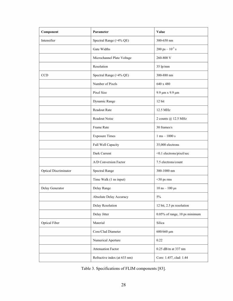
28

Component Parameter Value

Intensifier Spectral Range (>4% QE) 300-650 nm

Gate Widths 200 ps – 10-3 s

Microchannel Plate Voltage 260-800 V

Resolution 35 lp/mm

CCD Spectral Range (>4% QE) 300-880 nm

Number of Pixels 640 x 480

Pixel Size 9.9 μm x 9.9 μm

Dynamic Range 12 bit

Readout Rate 12.5 MHz

Readout Noise 2 counts @ 12.5 MHz

Frame Rate 30 frames/s

Exposure Times 1 ms – 1000 s

Full Well Capacity 35,000 electrons

Dark Current <0.1 electrons/pixel/sec

A/D Conversion Factor 7.5 electrons/count

Optical Discriminator Spectral Range 300-1000 nm

Time Walk (1 ns input) <30 ps rms

Delay Generator Delay Range 10 ns – 100 μs

Absolute Delay Accuracy 5%

Delay Resolution 12 bit, 2.5 ps resolution

Delay Jitter 0.05% of range, 10 ps minimum

Optical Fiber Material Silica

Core/Clad Diameter 600/660 μm

Numerical Aperture 0.22

Attenuation Factor 0.25 dB/m at 337 nm

Refractive index (at 633 nm) Core: 1.457, clad: 1.44

Table 3. Specifications of FLIM components [83].

29

2.2.3 Rapid Lifetime Analysis

FLIM imaging and analysis was done via an intensified CCD camera controlled by the

DaVis 6 software (LaVision, Goettingen, Germany). A dark background was taken to

account for thermal current in the CCD and was subtracted from each intensity image.

The CCD camera is operated within its specified linear intensity-response range, which

was controlled by two separate settings: 1) Adjusting the gain on the intensifier via the

HRI and 2) modulating the gate width via the software interface. No adjustments were

made to the intensity images other than those during image capture.

Since fluorescence lifetimes must be calculated on a per pixel basis for FLIM, iterative

algorithms can be time-consuming and computationally intensive. Alternate approaches

such as Rapid Lifetime Determination (RLD) are more amenable for imaging systems

where speed/time is of value. The RLD approach in its simplest form (2-gates) is shown

in Fig. 7.

Figure 7: Illustration of lifetime determination for a single pixel with the 2-gate RLD approach.

Assuming an extremely short excitation pulse and a single exponential decay τ, imaged

with an ICCD gate width GW, the detected photon counts at any pixel is given by:

30

[ ] 100

/0

0

0

/0 .)( CeIdteICcounts GWt

tt

GWt

t

t =−=≈+−

+−∫ ττ τ (3)

Two consecutive points, given by total counts C1 and C2 (Fig. 7), then define the single

exponential decay:

⎟⎠⎞⎜

⎝⎛−

=

2

1

12

ln CC

ttτ (4)

2-gate schemes are susceptible to noise, so we extend our acquisition to multiple gates

and implement a version of the RLD that is extensible to an arbitrary number of gates.

Lifetime maps were calculated from multiple intensity maps on a per-pixel basis by

fitting the lifetime of pixel p to the logarithm of the intensity (assuming single-

exponential decay):

Ctt

Ip

ipi +−=,ln (5)

where Ii,p is the intensity of pixel p in image i, ti is the time delay of image i, and C is a

constant. Least squares lifetime fits were:

( ) ( )( )( )∑∑∑∑∑

−

−−=

piipii

iip ItItN

ttN

,,

22

lnlnτ (6)

where N was the number of images. All sums are over i. At each delay, the average of

five intensity images was recorded to compensate for excitation laser intensity. All

images were pre-processed via a uniform threshold filter where pixels below a minimum,

non-zero intensity value were set to zero. The nitrogen laser was operated at about 3 Hz

and 640×480 pixel lifetime images using 4 gates were generated using a PC with an Intel

Pentium-IV processor at 3.2 GHz, for total acquisition and analysis times <15 s. Accurate

lifetimes were obtained by creating a histogram based on the lifetime map, fitting it to

31

log-normal functions and calculating the average time from the regression. The resulting

image is the final lifetime map.

2.2.4 Noise Removal

Figure 8: Illustration of adaptive and baseline noise removal for a fluorescent structure (inner green circle) with haze (outer green circle). G1,G2,G3,G4 = Gated images 1-4. The inset square area denote the user-defined haze region. Note how it changes intensity for each gated image for adaptive technique, but retains the same value for the baseline approach.

ICCDs form an important component of low-light imaging systems, but also lead to loss

of spatial resolution. One issue with ICCD use is the lateral smearing of fluorescence,

which manifests in the form of haze around fluorescent structures. We have already

described how thermal and background noise is removed during image acquisition and

processing; here we describe two additional approaches which allow the User to pick and

remove haze as much as possible for 2D imaging. More sophisticated noise removal for

32

3D imaging via image restoration will be discussed in later chapters. Adaptive and

baseline noise removal is illustrated in Fig. 8.

4 gated images (i.e. taken at different delays) were acquired via FLIM and analyzed to

yield lifetime maps as described previously [70]. The lifetime macro was modified to

implement both adaptive and baseline haze removal.

a) Adaptive – The user was prompted to select a rectangular region representative of haze

in the first gated image (highest SNR). For each gated image then, the macro averaged

the pixel intensity in the selected rectangular area and subtracted the average value on a

per pixel basis from that gated image alone. The term ‘adaptive’ hence comes from the

fact that the haze removal from each gated image is dependent on that particular image

alone.

b) Baseline – The baseline approach is similar to the adaptive, except that the User

selected a haze area from the last gated image (lowest SNR), which was then averaged

and subtracted on a per pixel basis from ALL gated images. This approach is hence

equivalent to a single offset value applied to all gated images.

Since haze is almost always greater than background noise, both adaptive and baseline

methods also serve to remove background and, to some extent, dim defocused

fluorescence as well.

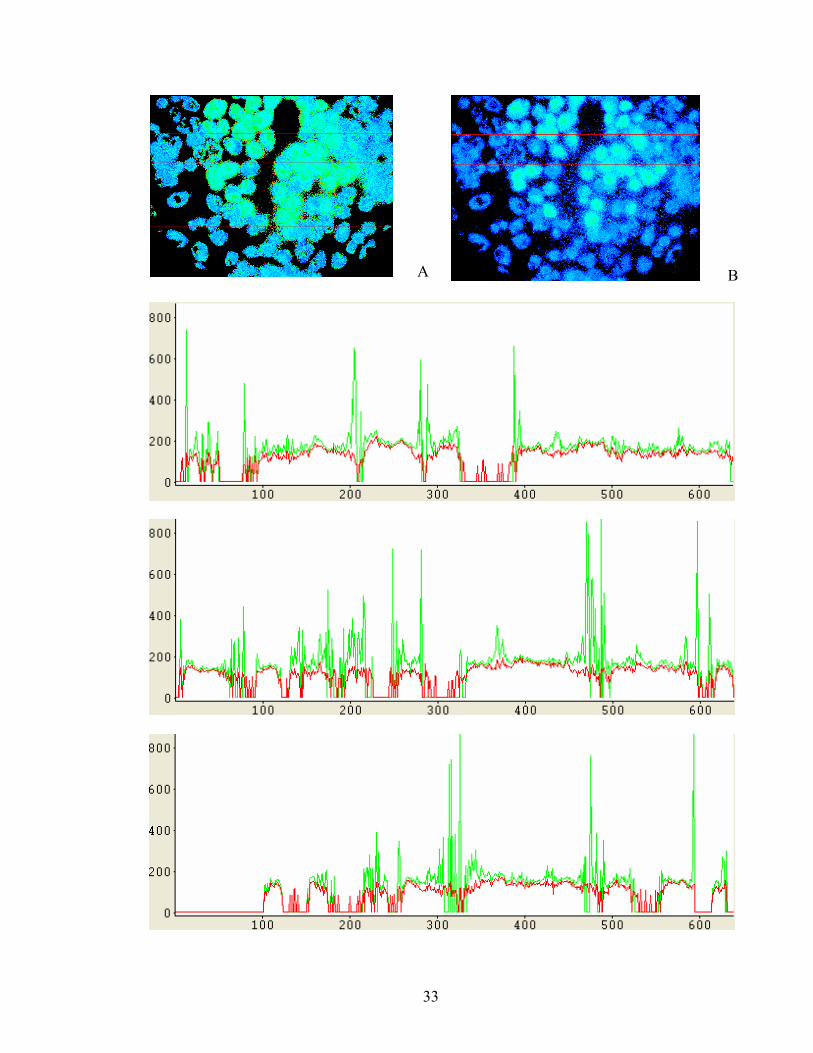
33

A B

34

Figure 9: Comparison of adaptive (A) and baseline (B) approaches applied to images of RTDP-labeled living adenocarcinoma (SEG) cells. Line profiles are shown are shown for three lines as plots of lifetime (hundreds of ns, y-axis) and pixel number (x-axis), for both adaptive (green lines) and baseline (red lines) approaches. The effect of both baseline and adaptive haze removal on a fluorescence lifetime image

of living SEGs incubated with RTDP is shown in Fig. 9. Also illustrated are the lifetime

values at three different horizontal profiles within the image. Several differences between

the two methods are evident from the images. Firstly, haze and background removal is

more effective for the adaptive approach. As a result spatial resolution is slightly better

for the adaptive approach as well. Secondly, the lifetime profiles for the adaptive

approach show significant spikes of inordinately high value and are likely inaccurate.

Notably, the ‘spiky’ values are seen only on the boundaries of the fluorescent cells,

something observable with other samples too (data not shown). The lifetime profiles for

the baseline image, on the other hand, are relatively flat and require no filtering for

spikes. Lastly, it is observable that lifetime values for the baseline approach are lower as

compared to the adaptive approach. This is again consistently observed for any

fluorescent sample, and is a property of the difference in analysis between the adaptive

and baseline approaches.

For a more mathematical reasoning of these observed differences, we can use a simple 2-

gate model of single-exponential decay (as described earlier), lifetime at any given pixel

can be evaluated as:

⎟⎠⎞⎜

⎝⎛−

=

2

1

12

ln CC

ttτ (7)

35

Where t2 (second gate) > t1 (first gate), and hence intensity counts C1 > C2. With adaptive

haze removal, a variable intensity value (say x1, x2) that is is subtracted from every pixel:

⎟⎠⎞⎜

⎝⎛

−−

−=

22

11

12

ln xCxC

ttτ (8)

Since C1>C2 and x1>x2, the ln term does not undergo significant change and lifetime

information is generally conserved. With baseline haze removal, a fixed intensity value

(say ‘x’) is removed from every pixel:

⎟⎠⎞⎜

⎝⎛

−−−

=

xCxC

tt

2

1

12

lnτ (9)

The denominator can be rewritten as:

⎥⎥⎥

⎦

⎤

⎢⎢⎢

⎣

⎡

−

−∗⎟⎠⎞⎜

⎝⎛=

2

1

2

1

1

1ln

Cx

Cx

CC (10)

⎥⎥⎥

⎦

⎤

⎢⎢⎢

⎣

⎡

−

−+⎥⎦

⎤⎢⎣⎡

⎟⎠⎞⎜

⎝⎛=

2

1

2

1

1

1lnln

Cx

Cx

CC (11)

It follows that:

01

1ln

2

1 >⎥⎥⎥

⎦

⎤

⎢⎢⎢

⎣

⎡

−

−=

Cx

Cx

(12)

The additional positive term in the denominator results in a decrease in estimated

lifetime, which explains why the baseline process consistently yields lower lifetime

values than the adaptive approach. The additional term also likely explains the edge

effect/spiky lifetime values; at low SNR, C1 is only slightly higher than C2, so C1/C2 is

close (but never equal) to 1, hence ln(C1/C2) is close to 0. This explains the inordinately

36

high lifetime values seen with the adaptive approach. Due to the additional ln [(1-

x/C1)/(1– x/C2)] denominator term in the baseline approach, this effect is mitigated, at the

cost of resolution and limited error in lifetime determination.

For all work reported in this dissertation, the adaptive noise removal approach was used.

Spiky lifetime values were removed by setting the pixel lifetime value to zero. Given the

flexibility of the imaging algorithm, it is quite possible to use alternate actions (e.g. set

pixel value to image average or to a programmable maximum value).

37

Chapter 3 INTRACELLULAR OXYGEN SENSING IN LIVING CELLS

3.1 Introduction Cancer mortality presents one of the leading medical challenges in the United States,

accounting for almost 25% of all deaths [84]. While research has been extensive in this

area, loss of life due to cancer was unchanged from 1950 to 2002 (193 deaths per

100,000), a trend explained to some extent by increased diagnosis and awareness in the

general populace [84]. Cancer prevention through lifestyle changes and early detection is

the most effective means of lowering these mortality rates.

Given the success of endoscopy as a minimally-invasive imaging modality for early

cancer detection in the esophagus, the identification of an optically discernable

mechanism that is consistently altered in a malignant process could prove very useful, not

only for further developing therapeutic targets, but also for understanding disease

pathogenesis and developing minimally invasive optical technologies for early detection.

A recent clinical study presented evidence for the presence of detectable levels of

NAD(P)H fluorescence in human epithelial tissues in vivo and demonstrated that

NAD(P)H may be used as a quantitative fluorescence biomarker for in vivo detection of

dysplasia in the esophagus [51]. Here, the underlying biological basis for endogenous

38

fluorescence changes that occur during the course of esophageal cancer progression was

investigated by employing a unique, time-resolved optical molecular imaging approach

that provides a molecular snapshot of metabolic function in living human esophageal

cancer cell models.

Knowing the complicated nature of cellular machinery, it is not surprising that pervasive

changes in metabolic function almost always manifest as ill health at the anatomic level.

The oxidative phosphorylation cycle is an attractive point of analysis in this regard:

several key biomolecules such as NAD(P)H, FADH2, oxygen, and ATP are

consumed/generated during this process. Of these, NAD(P)H provides a bright,

endogenous fluorescence signature that is detectable optically without the use of

exogenous dyes [85]. Oxygen, while not fluorescent, can quench fluorescence in

transition-metal complexes [11] and a class of ruthenium dyes has emerged as the

biological probe of choice for oxygen sensing that has been studied for photochemistry,

oxygen response, and toxicity [86, 87].

The large temporal dynamic range (600 ps – infinity) of FLIM are unique and essential

for the purpose of this study: UV excitation and an ultrafast gated camera enable imaging

of endogenous fluorophores such as NAD(P)H with sub-nanosecond lifetimes, while

visible excitation from a low repetition rate laser source and large gates enable measuring

lifetimes for ruthenium dyes, which are typically hundreds of nanoseconds. FLIM has

been successfully applied to the study of NAD(P)H fluorescence, as well as lifetime

modulation of oxygen sensitive ruthenium tris(2,2’-dipyridyl) dichloride hexahydrate

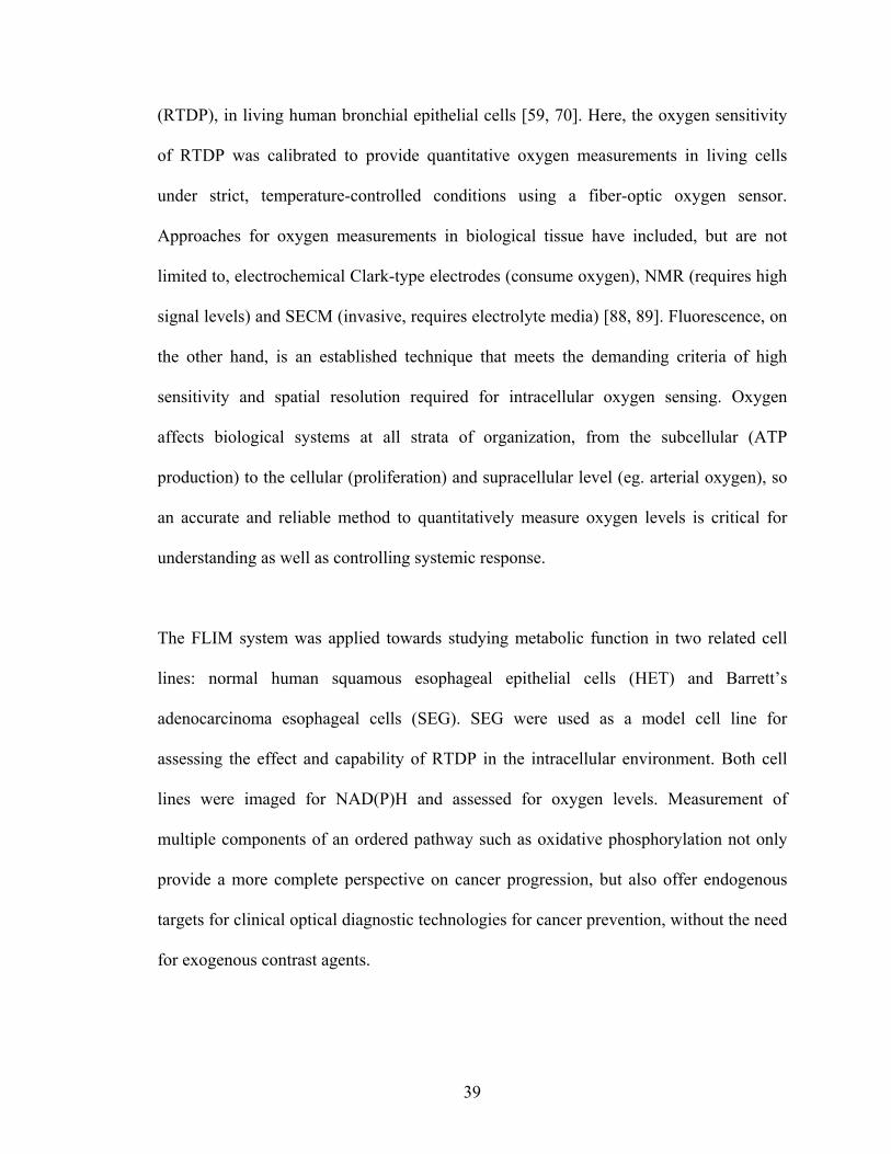
39

(RTDP), in living human bronchial epithelial cells [59, 70]. Here, the oxygen sensitivity

of RTDP was calibrated to provide quantitative oxygen measurements in living cells

under strict, temperature-controlled conditions using a fiber-optic oxygen sensor.

Approaches for oxygen measurements in biological tissue have included, but are not

limited to, electrochemical Clark-type electrodes (consume oxygen), NMR (requires high

signal levels) and SECM (invasive, requires electrolyte media) [88, 89]. Fluorescence, on

the other hand, is an established technique that meets the demanding criteria of high

sensitivity and spatial resolution required for intracellular oxygen sensing. Oxygen

affects biological systems at all strata of organization, from the subcellular (ATP

production) to the cellular (proliferation) and supracellular level (eg. arterial oxygen), so

an accurate and reliable method to quantitatively measure oxygen levels is critical for

understanding as well as controlling systemic response.

The FLIM system was applied towards studying metabolic function in two related cell

lines: normal human squamous esophageal epithelial cells (HET) and Barrett’s

adenocarcinoma esophageal cells (SEG). SEG were used as a model cell line for

assessing the effect and capability of RTDP in the intracellular environment. Both cell

lines were imaged for NAD(P)H and assessed for oxygen levels. Measurement of

multiple components of an ordered pathway such as oxidative phosphorylation not only

provide a more complete perspective on cancer progression, but also offer endogenous

targets for clinical optical diagnostic technologies for cancer prevention, without the need

for exogenous contrast agents.

40

3.2 Materials, Instrumentation, and Methods

3.2.1 Fluorescence Lifetime Imaging Microscope (FLIM)

150

200

250

300

350

400

450

0 1 2 3 4 5

RTDP Conc. (mg/ml)

Inte

nsity

(cou

nts)

and

Li

fetim

e(ns

)

Lifetime(ns)

Intensity(counts)

A

y = 0.0044x + 1.0346R2 = 0.9862

0

0.5

1

1.5

2

2.5

0 50 100 150 200 250 300Oxygen (μM)

Rel

ativ

e Li

fetim

e (τ

0/τ)

B Figure 10: A) Plot of RTDP intensity (pink squares) and lifetime (blue diamonds) vs. RTDP concentration. Lifetime was contant over a large range, while intensity varied with concentration before saturating. B) RTDP Calibration Curve: Plot of relative lifetime (τ0/ τ) vs. oxygen levels (μM). RTDP calibration indicated a linear relationship between oxygen levels and relative lifetime, which was in good agreement with the Stern-Volmer equation. Over multiple runs Kq = 4.5±0.4x10-3 µM-1.The intercept ≠ 1, indicating some degree of experimental variance. The calibration could differentiate between oxygen levels differing by as little as 8µM.

41

The FLIM system has been described in Chapter 2. For RTDP experiments, a dichroic

mirror (Q495lp, Chroma Technology Corp., Brattleboro, VT) delivered the beam into a

40× Fluar (1.3NA, Zeiss, Jena, Germany) objective for sample excitation with an

illumination diameter of 150 μm. Gate widths were controlled by slaving the ICCD gate

to an external logic signal. Intensifier (MCP) voltage was set at 700 V for the RTDP

solution and 800 V for cell samples. For imaging cellular NADH, the ICCD was operated

in Comb mode and the dichroic mirror (350lpDC Chroma Technology Corp.) was

changed accordingly.

3.2.2 Image Analysis Image acquisition and processing for FLIM was described in Chapter 2. For RTDP

imaging, the linear scale of the lifetime map was converted to a binary, two-color scale

for the sole purpose of easier visualization. The oxygen distribution image was generated

by directly applying the calibration (described below) to the lifetime map without pre-

processing. Finally, threshold filters were applied that set pixels with unlikely oxygen

levels (both low and high) to zero. This is reasonable given the range of physiological

oxygen values [90].

3.2.3 Temperature Control For temperature control, the Delta T controlled culture dish system (Bioptechs, Butler,

PA) was implemented along with the Delta T perfused heated lid (Bioptechs) and was

used for all experiments, unless noted otherwise. The heated lid had two ports which

could be used for perfusion purposes. A remote controller was used to adjust temperature

settings. For closed chamber experiments the FCS2 chamber system and controller

42

(Bioptechs) was used, where cells were enclosed between a cell plate and a perfusable

gasket with a media holding capacity of 1 ml. Due to the large thermal mass of the

objective, a separate Objective Heater (Bioptechs) with its own controller was also

installed. All temperature control systems had an operating range from ambient to 45°C

with accuracy within ±0.2°C.

3.2.4 Confocal Microscopy An independent Zeiss LSM 510 microscope (Zeiss, Jena, Germany) was used to acquire

confocal NADH fluorescence images via 364 nm excitation (emission: 435 nm-485 nm).

Images were acquired via LSM 5 Software Release 3.2 (Zeiss) in real time. Detector gain

and offset were configurable via the software interface and were adjusted to avoid

detector saturation. Offline image analysis was done using LSM Image Browser 3.2

(Zeiss). The only image parameters adjusted for enhancement were brightness and

contrast and these changes were uniformly applied across the entire image. A range

indicator function in the software provided information on color saturation (via

brightness enhancement) or zero pixel values (via increased contrast). The function used

a pseudo-color scheme where all saturated pixels were colored red, all zero pixels were

colored blue and all other were plotted on a linear grayscale. Adjusting brightness and

contrast while maintaining the entire image within the grayscale range allowed

preservation of image information while avoiding loss or generation of data.

3.2.5 RTDP Characterization

0.025 g of RTDP (ruthenium tris(2,2’-dipyridyl) dichloride hexahydrate) powder

obtained from Sigma-Aldrich (#224758, St. Louis, MO) was dissolved in 25 ml

43

phosphate buffer saline (PBS, Invitrogen, Carlsbad, CA) to create a stock solution of 1

mg/ml, or 1.34 mM. Absorption spectra of RTDP were obtained from a Beckman-Coulter

DU-800 Spectrophotometer (Ontario, Canada) over a range of 200-800 nm. The

fluorescence emission spectrum was extracted using a Jobin-Yvon Fluorolog-3 (Edison,

NJ) in a range of 300-700 nm. Temperature response of RTDP lifetime was studied using

2 ml of stock solution and FLIM. Initially, ambient temperature was 22°C and the

solution was exposed to normal atmospheric conditions. Temperature was varied in the

range of 25-45°C in steps of 2.5°C. At each temperature point, lifetime images were

acquired three times and averaged. Multiple runs were used to validate the slope of the

plot obtained. FLIM was used to study RTDP lifetime independence of its concentration.

Six different RTDP concentrations in the range 0.5-5 mg/ml were used for intensity and

lifetime studies (Fig. 10A). The temperature was set to 37°C (physiologic value), gate

width at 50 ns and the HRI gain at 700 V. The settings were selected to maximize signal

at the CCD without saturation when the highest concentration of 5 mg/ml was measured

for lifetime. Below 0.5 mg/ml, the intensity was too weak to reliably evaluate lifetimes

without changing gain settings to manipulate intensity. Three readings were obtained per

concentration and were averaged for intensity and lifetime.

3.2.6 Calibration of Oxygen Sensitivity of RTDP Independent oxygen measurements for RTDP calibration were performed using a

commercial fiber-optic oxygen sensing system (FOXY, Ocean Optics, Dunedin, FL). The

FOXY system is a fluorescence-based, spectrometer-coupled chemical sensor used for

spectral analysis of both dissolved and gaseous oxygen with a manufacturer specified

range of 0-40 ppm (>1 mM) for oxygen dissolved in water, a resolution of 0.02 ppm, and

44

response time < 1 sec. The FOXY was calibrated using a two-point linear fit. The first

point was obtained by immersing the FOXY probe in a solution of sodium hydrosulfite

(dithionite) dissolved in DI water through which nitrogen had been bubbled, yielding a

solution with near-zero oxygen concentration (sodium dithionite is a potent oxygen

scavenger and bubbling nitrogen removed virtually any traces left). The second point was

obtained by immersing the FOXY probe in a solution of DI water, which has a known

oxygen concentration of 7.1 ppm or 222 μM at 37°C under normal atmospheric O2. Data

from these two points was used to calibrate the FOXY via a software interface.

Next, a lifetime-oxygen calibration of RTDP was performed on the stock solution using

FLIM. Gas tubing was attached to one port on the heated, perfused lid while the FOXY

was inserted into the solution via the other port. Under equilibrium conditions, the

oxygen level was similar to the calibration value, i.e., 7.1 ppm. Nitrogen was flowed over

the sample and a drop in oxygen was recorded via FOXY. Once the FOXY output

stabilized at <0.1 ppm, the lifetime was recorded, the flow of nitrogen was stopped and

the solution was allowed to recover by equilibrating with atmospheric oxygen. During

this process, several concurrent lifetime and oxygen measurements were taken.

Once the solution reached equilibrium, the solution was perfused with oxygen and an

increase in levels was correspondingly observed by the FOXY. The oxygen flow was

then cut-off and while the solution stabilized toward equilibrium, readings were taken in

a manner similar to that described above. The data was verified by repeating the

calibration multiple times. Average values were used for cell studies.

45

Data analysis - Stern-Volmer Equation: Oxygen is one of the best known collisional

quenchers and its effect on RTDP can be effectively described by using the Stern-Volmer

Equation [11]. Since increased temperatures lead to faster diffusion for both fluorophore

and quencher and hence higher collision quenching rates, it is characteristic for Kq to

increase with temperature [11]. To evaluate Kq, the highest lifetime value attained (when

[O2] <0.1 ppm) was set equal to τ0. This was reasonable, since the FOXY had a minimum

detection limit of 0.02 ppm and it is near impossible to completely deplete oxygen. For

all other values, τ0/ τ was evaluated and plotted as a function of [O2]. Line fitting of all

data points and regression analysis was carried out using statistical software. The slope of

the line yielded a single value of Kq. Over multiple runs, Kq was averaged to provide a

mean value that was used for analyzing cell lifetimes (see below). A key advantage of the

relative lifetime, Stern-Volmer approach was that any variability in RTDP lifetime

associated with aging or other ambient conditions was systematically eliminated by

determining τ0 from the known (stock) solution for each experiment.

3.2.7 Cell Preparation The HET-1 is a human squamous epithelial cell line immortalized by transfection of the

SV40 T antigen early region gene [91]. The SEG-1 (Barrett’s) adenocarcinoma

esophageal cell line was derived from Barrett’s-associated adenocarcinoma of the distal

esophagus [92]. HET and SEG were propagated in 100 cm2 culture flasks in DMEM

media (Invitrogen) containing 10% fetal bovine serum (FBS) and cultured at 37°C under

standard conditions. Upon reaching 70% confluence, the cell cultures were split using

trypsin and divided at a ratio of 1:4. For open-air studies, the cells were plated a day

before experimentation. About 6 hours before analysis, 1 ml of RTDP stock solution was

46

added to the cells. The cells were washed with PBS or media (without phenol red) before

being transferred to the microscope stage. This process was mirrored for both cell lines

whenever comparative studies were done. Cell viability tests (Trypan Blue) yielded

>85% viability after 6 hrs of incubation with RTDP, indicating that significant

cytotoxicity was not occurring within the incubation period. No staining was necessary

for NADH studies.

For closed chamber RTDP studies, the cells were plated a day before on cell plates (see

Temperature Control) and the RTDP stock solution was added about 6 hours before

experimentation. After washing with PBS, the plates were assembled into the closed

chamber system, sealed shut with media and mounted onto the microscope stage.

3.2.8 RTDP Lifetime Measurement in Cells All controllers were set at 37°C after the cells were loaded onto the stage. The objective

was used to focus on an appropriate region with the cells clearly visible and lifetime

measurements were taken. Each measurement was repeated multiple times. For time-

lapse experiments, measurements were taken periodically. Lastly, for each experiment,

the lifetime of the stock solution was also obtained. The calibration (Kq) was applied to

determine intracellular oxygen concentration. Values of lifetime (τ) was evaluated for the

stock solution of known oxygen level and fed into the Stern-Volmer equation to obtain τ0.

A software macro was implemented to generate oxygen distribution images based on the

calibration data and using the lifetime images as input. The oxygen distribution was

evaluated on a pixel by pixel basis for each lifetime image by feeding back the value of τ

into the Stern-Volmer equation. For each cell visible in the lifetime image, τcell was

47

evaluated as the average of all pixels comprising the image of the cell. Hence, oxygen

levels were assumed to be uniform within a cell. Average intracellular oxygen levels

were evaluated from the oxygen distribution in a similar manner. For each experiment,

oxygen levels from at least 5 cells were averaged to obtain mean values.

48

3.3 Results

3.3.1 NADH Measurements in HET and SEG

A

B C

D E

13 40

2.512.21

0

10

20

30

40

50

60

HET SEG

NA

DH

Inte

nsity

0

1

2

3

4

5

6

NA

DH

Life

time

(ns)

IntensityLifetime

F

49

Figure 11: A) Oxidative phosphorylation in mitochondria. Complex I (NADH dehydrogenase) converts NADH to NAD+ and passes on electrons to carrier CoenzymeQ (CoQ) while pumping hydrogen ions into the intermembrane space. Complex II (succinate dehydrogenase) can also generate and pass on electrons to CoQ via a complex internal mechanism which is initiated by conversion of succinate to fumarate, a step in the Krebs cycle. CoQ transfers the electrons to an intermediary complex III (CoQ – cytochrome C oxidoreductase), which in turns enhances the proton gradient by pumping hydrogen ions against the gradient. The electrons are transferred to complex IV (cytochrome oxidase) via cytochrome C (CytC) which in turn hydrolyses oxygen to water and also pumps protons against the gradient. The ATP synthase complex (complex V) moves protons down the gradient, converting osmotic energy to chemical energy via ATP synthesis from ADP in a process known as chemiosmotic coupling. A more detailed explanation of the process and the unique structure of ATP synthase can be found in any standard biochemistry text. B) NADH fluorescence and C) Mitotracker-stained SEG images. For the Mitotracker, excitation = 543 nm and emission = 636 nm. Mitotracker Red is a commercially available stain used for tracking mitochondria within living cells. Fluorescent signals from both markers were found to co-localize. Confocal intensity images of NADH fluorescence in HET (D) and SEG (E): Illustration of differences observed with the Zeiss 5 LSM. The SEG consistently presented a brighter signature than the HET by approximately 2.5-fold. F) Plot of differences in NADH fluorescence intensity and lifetime observed between the HET and SEG over multiple measurements with the FLIM system. No significant differences in NADH lifetime were observed.

NADH reduction by complex I to NAD+ along with electron transfer to the carrier

coenzyme-Q (CoQ) is one of the first steps in oxidative phosphorylation (Fig. 11A). This

step contributes not only to oxygen consumption downstream but also to the proton

gradient which ultimately results in ATP production. Since NADH is generated during

glycolysis and consumed during oxidative phosphorylation, it is one measure of

completion for these processes.

The term NAD(P)H is used to point out the spectral similarity of NADH and NADPH,

both of which have a wide excitation range centered at approximately 350 nm and an

emission peak at 460 nm. Since other endogenous fluorophores have overlapping

excitation in the UV range, preliminary studies were conducted to observe the sub-

cellular origin of fluorescence. Fig. 11 presents confocal fluorescence intensity images of

SEG incubated with a commercial mitochondrial stain (Mitotracker Red). Fig. 11B shows

50

that NAD(P)H fluorescence clearly has the same origin as the Mitotracker fluorescence

(Fig. 11C), indicating that fluorescence observed arose mostly from mitochondrial

NADH and not NADPH.

Figs. 11D, 11E provide confocal NADH fluorescence intensity images from HET and

SEG, respectively, under identical measurement settings. It is visually evident that the

SEG have a starkly brighter fluorescence signature than the HET. Similar results were

also obtained with FLIM and overall the SEG exhibited 2-5 fold higher fluorescence

signals than the HET. This difference in signal from NADH was observed to be

statistically significant (p<0.05, Fig. 11F).

FLIM measurements were made for NADH lifetime in both cell lines. Values obtained

were τHET = 2.51 ± 0.16 ns and τSEG = 2.21 ± 0.16 ns and were within the range of values

reported in literature [93]. The differences in lifetimes were not statistically significant,

therefore it can be established that the fluorescence intensity differences between the

HET and the SEG were mainly attributable to differences in intracellular NADH levels.

The observation reported here that esophageal cancer cells have higher absolute NADH

levels than normal esophageal cells could explain the higher levels of NAD(P)H reported

in dysplastic vs. nondysplastic esophageal tissues via clinical studies described earlier

(see introduction) [51].

3.3.2 RTDP Calibration RTDP has been studied for its photophysical and photochemical properties and recently

found application in biomedical research as a molecular oxygen sensor [86]. With a long

51

fluorescence lifetime (hundreds of nanoseconds), easy uptake by cells, and minimal

cytotoxic and phototoxic effects, RTDP provides a nearly ideal means of assessing

intracellular oxygen.

Measurements made with the FLIM system indicated that RTDP lifetime decreased with

increasing temperature and that this decrease was almost linear:

τ = -4.4975*T + K, r2 = 0.9867 (13)

where τ = lifetime and T = temperature in degree Celsius and K was a constant,

emphasizing the need for temperature control in lifetime studies. The slope was in good

agreement with previous work, which measured RTDP lifetimes within a similar

temperature range [87].

RTDP calibration results at 37°C indicated a linear relationship between oxygen levels

and relative lifetime, which was in good agreement with the Stern-Volmer equation (Fig.

10B):

τ0/ τ x = 1 + Kq[O2]x (14)

where Kq is the Stern-Volmer quenching constant. Relative lifetime at a given oxygen

level [O2]x was evaluated as the ratio of uninhibited RTDP lifetime (i.e. 0% oxygen, or τ

0) to τ x. Over multiple runs, the value of Kq was evaluated to be Kq = 4.5±0.4 x 10-3 μM-1.

This is higher than other reported values which were measured at room temperature,

confirming that Kq increases with temperature [90]. System resolution was determined by

a) the resolution of the oxygen sensor used for calibration (±0.6 μM) (see Methods

section) and b) the lifetime variance of the FLIM system (±2% of lifetime, or ±6 ns for

52

RTDP). Using these values in Eq. 14, it was estimated that the calibration could reliably

differentiate between oxygen levels differing by as little as 8 μM.

53

3.3.3 Oxygen Measurements in HET and SEG

A B

C D

E F

270

275

280

285

290

295

300

305

310

315

0 10 20 30 40 50 60Time(mins)

Life

time(

ns)

200

210

220

230

240

250

260

270

Oxy

gen(μM

)

LifetimeOxygen level

G

54

Figure 12: (A) confocal fluorescence and (B) Differential Interference Contrast, or DIC images of SEG. SEG were incubated with the RTDP dye prior to imaging (see Methods section). FLIM images of SEG incubated with RTDP: (C) DIC, (D) fluorescence intensity (0-400 counts), (E) lifetime (0-1000 ns) and (F) oxygen (0-500 µM). Note that one cell in the bottom of (C) shifted position in (D) in the time lapse between these two images. (G) The results of depletion experiments on SEG (see Methods section). Cellular viability is compromised with the passage of time and this results in the lifetime / oxygen content leveling off towards the end.

Confocal measurements indicated that RTDP distributed uniformly in the cytoplasm

without any evident aggregation or adherence to organelles (Fig. 12A,B). It yielded a

strong intracellular luminescent signal without visible cytotoxic effects or membrane

damage. Similar results were obtained with the FLIM system for both HET and SEG with

excellent cell viability (>85%).

Fig. 12C-F presents representative images of SEG cell lines after analysis for lifetime and

oxygen levels. The cell positions (C) overlaps with RTDP fluorescence (D). Note that the

fluorescence intensity image (D) is non-uniform, indicating that the cells differentially

absorb RTDP. The lifetime map (E) generated from the intensity map (D) indicated a

clear uniformity across different cells, signifying similar oxygen levels and reflecting

intensity independence of lifetime. RTDP calibration was used to generate an oxygen

distribution map (F) that implied uniform oxygen levels of approximately 285 μM. The

oxygen levels were found to be [O2]SEG = 260.16 ± 17 μM. While higher than reported in

vivo values, these levels were comparable to values generally observed in living

biological samples during ex vivo measurements. This is a leap forward from

measurements of extracellular oxygen alone, which assume linear correlation with

intracellular oxygen. Gradients between intracellular compartments and extracellular

space are known to exist but cannot be explained by simple diffusion rates alone [59, 90].

55

Time-lapse FLIM measurements were made on SEG under airtight conditions to verify

that decrease in oxygen levels due to cellular consumption would be reflected in RTDP

lifetime increase. The results are plotted in Fig. 12G. As expected, RTDP lifetime

increased by 35 ns over the course of an hour, reflecting a decrease in oxygen levels (Δ

≈-50 μM) due to gradual consumption by cells. These experiments demonstrate the

sensitivity of FLIM for oxygen sensing in living cells.

56

A D

B E

C F

182.1

260.5

0

50

100

150

200

250

300

HET SEG

Oxy

gen

(μM

)

G

57

Figure 13: RTDP fluorescence intensity (0-600 count) (A,B), lifetime (0-1000 ns) (C,D) and oxygen (0 – 500 μM) (E,F) maps of HET (A,C,E) and SEG (B,D,F). The intensity images (A,B) could not be reliably used to discriminate between the two different cell lines. The binary lifetime maps (C,D), on the other hand, plainly indicate different lifetimes for these two cellular species, with the SEG recording lower lifetimes than the HET. For the given case, τHET = 225 ns and τSEG = 170 ns. The mean lifetime difference was found to be Δτ = 44 ± 7.48 ns. Logically, this translated into higher oxygen levels in the SEG vs. the HET using the calibration derived earlier, as can be seen in the oxygen distribution maps (C,F). G) illustrates the differences in oxygen levels within the HET and SEG as measured over multiple runs and assessed using the RTDP calibration. The mean difference between the two cell lines was hence evaluated as Δ[O]2 = 78 ± 13 µM and this value was statistically significant (p< 0.001).

RTDP calibration was applied to measure quantitative differences in intracellular oxygen

between HET and SEG. Fig. 13A-F presents comparative images of HET (A,C,E) and

SEG (B,D,F) incubated with RTDP. Intensity images (A,B) do not yield any useful

information. Lifetime maps (C,D) are plotted on the same bicolor lifetime scale to better

illustrate disparities: the SEG clearly exhibit lower lifetimes than the HET, which in turn

translates to higher oxygen levels (E,F). This trend was consistent, with [O2]HET = 182.08

± 9.38 μM and [O2]SEG = 260.16 ± 17 μM (Fig. 13G). The difference between [O2]HET

and the extracellular media (222 μM) was within the range of gradients reported in

literature for various other cell models [94, 95]. Interestingly, the opposite trend is

observed in the SEG. The difference between HET and SEG for the images provided was

approximately 60 μM.

3.4 Discussion Patients diagnosed with esophageal cancer have one of the lowest 5-year survival rates

(14%) [84]. Several reports describe the use of endogenous tissue fluorescence (e.g.,

autofluorescence from NAD(P)H, collagen, FAD) as a biomarker for dysplasia in the

esophagus, and recent studies have corrected for signal distortions from other sources

58

(e.g., hemoglobin absorption) to yield quantitative trends (differences) between

fluorescence signatures of NAD(P)H and collagen in normal and dysplastic tissue in vivo

[51, 96, 97]. Thus, it was possible to observe consistent changes in absolute NAD(P)H

and collagen fluorescence levels of multiple patients and accurately correlate them with

the degree of neoplastic change [51]. A key strength of tissue spectroscopy is the

acquisition of data in the appropriate local environment. Although cellular NAD(P)H is a

marker of esophageal cancer progression, the exact mechanisms are unknown in part due

to the poor spatial resolution of fiber-optic based spectroscopic measurements. Thus,

spectroscopy is unable to distinguish between cellular NADH in mitochondria and

NADPH in the cytoplasm, due to their spectral similarity (hence the term NAD(P)H).

Both these components, however, have contrary roles: NADH takes part in the electron

transport chain in mitochondria to generate ATP, while NADPH is the reducing agent for

anabolic reactions such as fatty acid synthesis that consume ATP. This article reports

results from a dual confocal-FLIM approach towards measuring NAD(P)H fluorescence

in cell models characteristic of normal and adenocarcinoma esophageal state (HET and

SEG, respectively). High resolution confocal images of NAD(P)H and Mitotracker

fluorescence (Fig. 13B,C) provided sub-cellular imaging of co-localization of these two

signals, indicating that endogenous fluorescence arose primarily from mitochondria and

was NADH. Using FLIM, differences in NADH fluorescence intensity were observed

between HET and SEG, while there was no significant variation in NADH lifetime

between cell lines (Fig. 13F), indicating that differences in fluorescence intensity were

mainly attributed to differences in NADH concentration, and did not arise from

fluorescence quenching. Intensity results were corroborated with the confocal system

59

(Fig. 13D,E) and confirmed that SEG contained significantly higher NADH levels than

the HET, a trend similar to and supporting clinical observations.

Elevated NADH levels in SEG raises the question whether it is being excessively

produced during glycolysis or consumed less due to possible mitochondrial dysfunction.

Mitochondria provide a more logical starting point for further analysis: they are well

characterized, complex organelles which play key roles in several cellular functions such

as fatty acid metabolism, calcium homeostasis and most importantly, ATP production via

the oxidative phosphorylation (OXPHOS) pathway (Fig. 13A) [98]. It is clear that

defects/alterations in OXPHOS enzymes have links to some forms of cancer,

neurogenerative diseases, diabetes and aging [98, 99]. The first step in OXPHOS

involves the reduction of naturally fluorescent NADH to its non-fluorescent analog

NAD+ via the membrane-bound complex I enzyme. Given the sequential nature of

OXPHOS, it is logical that variations in NADH will affect the rate of downstream

processes; i.e., consumption of oxygen and generation of ATP. ATP is the energy

currency of the cell but is not an intrinsic fluorophore and commercial fluorescence

indicators for ATP do no differentiate between ADP and ATP, making analysis difficult

[100]. Oxygen, on the other hand, is likely the most pertinent indicator of completion of

cellular respiration, in general, and OXPHOS, ATP production, in particular.

Experiments conducted on HET and SEG indicated the potential of RTDP as an oxygen

sensitive ruthenium dye that was well tolerated by living cells and yields a bright

fluorescence signal to provide a molecular capability for analyzing intracellular oxygen

levels in these cell models (Fig. 13A-F). After calibrating the oxygen sensitivity of RTDP

60

lifetime via FLIM, modulation of intracellular RTDP lifetime was demonstrated via the

gradual depletion of oxygen supply to SEG (Fig. 13G). Using FLIM, it was estimated

that [O2]SEG = 260.16 ± 17 μM under cell culture conditions. Oxygen levels in HET were

lower than SEG, observed as [O2]HET = 182.08 ± 9.38 μM, bearing an average difference

Δ[O2]SEG-HET ≈ 80 μM (Fig. 13A-G). This difference was statistically significant

(p<0.05). It is important to note that cells in culture are exposed to higher oxygen levels

than in vivo (especially for cancer cells which normally inhabit a hypoxic environment in

vivo) and their behavior under these conditions can be meaningfully interpreted to

understand causal behavior. This comparative tactic of tracking differences between

normal and altered cell lines is easily extensible to other disease models and/or analytes

other than NADH and oxygen.

The phototoxicity of RTDP in living cells was extensively documented previously [86].

The protocol used in that study included supplementation of the culture media by a

solution of RTDP immediately prior to 457 nm excitation in a Bio-Rad MRC1024 laser

scanning confocal system. Based on the data provided, we estimate that each illumination

delivered approximately 0.8 J/cm2 of energy on the sample. Depending on the

concentration of RTDP used, photodamage to living cells occurred when the cumulative

light dose exceeded 20-80 J/cm2 (2-0.2 mM). In contrast, the protocol employed here

involved incubating the cells with 1.3 mM RTDP stock solution for 6 hours and washing

away the dye with PBS prior to experimentation. The intracellular concentration of

RTDP, while not measurable, was clearly lower than the stock solution as inferred from

intensity based fluorescence measurements. For the study described here, the laser pulse

61

energy at the sample was 15 μJ and the illumination area was approximately 0.5 mm in

diameter. Hence, the energy per unit area was 1.9 mJ/cm2 for a single measurement.

Further, the lifetime analysis protocol required intensity images captured at six different

delays, at five measurements per delay. Therefore, it required thirty measurements to

deduce lifetime, resulting in a total energy exposure of 0.057 J/cm2 at the sample. Lastly,

six lifetime measurements were taken for oxygen depletion experiments and the

cumulative energy deposited was 0.34 J/cm2. This is significantly lower than the

threshold observed previously [86]. Coupled with the extremely low levels of RTDP

being excited, we reasonably infer that the FLIM-based experiments presented here do

not cause photodamage.

The studies presented here confirm that optical measurements of fluorescence from

endogenous mitochondrial NADH might be useful for non-invasively detecting altered

metabolic function in esophageal cancers in vivo. Use of exogenous agents such as

RTDP, provide a complementary, highly specific approach for quantitative, intracellular

oxygen sensing in living cells. Results presented here indicate that a possible alteration in

cellular metabolism in SEG early in the OXPHOS pathway could cause decreased NADH

consumption (higher intracellular levels), which would then lead to lower oxygen

consumption downstream and hence elevated intracellular oxygen levels relative to HET,

as observed. While reports on basal cell carcinoma indicate that OXPHOS complex I

gene and/or protein modification might result in impaired activity, no such report was

found for esophageal cancers [101].

62

The flexibility of FLIM to detect endogenous cellular fluorescence from NADH, as well

as exogenous fluorescent tags and labels, makes the method compatible with endoscopic

clinical imaging studies in living human tissues. A large temporal dynamic range and a

microscopy imaging modality provide the ability of measuring both fluorescence and

phosphorescence with subcellular spatial resolution. High temporal resolution and single-

shot imaging aid in resolving molecular events such as conformational and viscosity

changes. Temperature and perfusion control of the cellular environment are beneficial for

viable cell imaging under physiologic conditions and to observe cellular response to

conditions such as hypoxia and heat shock. Further, thick biological specimens can be

imaged in layers by rejection of out of focus light (optical sectioning) via structured

illumination to yield 3-D distribution of analytes (e.g., oxygen gradients in thick tissues).

The oxygen sensing capability of FLIM was recently exploited to provide one of the first

few reports on oxygen gradients in microfluidic bioreactors containing living cells

(submitted).

The approach described here employed time-resolved optical imaging to probe metabolic

pathways in living cells using endogenous and/or exogenous fluorescence agents. A

calibrated approach for quantitatively estimating oxygen levels in HET and SEG using a

tunable, temperature-controlled FLIM was presented, with the potential to perform

absolute oxygen measurements in living biological systems with a resolution of 8 μM

over the entire physiological range (0-300 μM). Previous studies provided a calibration

curve for RTDP dissolved in growth buffer, but measurements were performed at room

temperature and were made using electrodes, which consumed oxygen and required

63

constant stirring of the media [90, 102]. Given the temperature-dependence of lifetime,

oxygen solubility, and cellular biochemical response, a controlled study like this provides

more accurate results. Precise measurements of intracellular oxygen provide important

information in areas such as pharmaceutical research or systems biology and may aid in a

better understanding of systemic disorders and their control.

64

Chapter 4 CALIBRATION AND VALIDATION OF INTRACELLULAR OXYGEN MEASUREMENTS

4.1 Introduction Oxygen is the terminal electron acceptor of oxidative phosphorylation in the

mitochondria and a key indicator of metabolic function in aerobic cells and organisms.

Information obtained from accurate oxygen estimation has been applied for studying

mitochondrial function, signaling pathways, effects of various stimuli, membrane

permeability, differentiation between normal and disease, or to screen for new drugs [94,

103-105]. Various methods exist for estimating oxygen at different scales, whether in

whole organs (MRI, NMR), in the blood (absorption), in tissues (electrochemical

microelectrodes) or in individual cells (phosphorescence, fluorescence, EPR) [54, 59,

106, 107]. Optical approaches such as fluorescence microscopy provide the most viable

approach for intracellular oxygen sensing with high sensitivity and spatial resolution.

Fluorescence lifetime-based methods additionally circumvent most issues associated with

intensity-based intracellular studies, such as photobleaching, scattering, variable uptake

by cells, etc [70].

Chapter 3 presented a FLIM-based approach for intracellular oxygen sensing using the

oxygen-sensitive dye RTDP. One concern that consistently arises is the validity of

65

applying an oxygen calibration derived in PBS solution to measurements made in living

cells, including how other intracellular factors might affect RTDP lifetime. Oxygen

sensitivity of RTDP is widely accepted and exploited [87]. It has been demonstrated that

RTDP lifetime is unaffected by solvent pH and ionic concentration (including Na+, Ca2+,

Cl-) within physiologic ranges, but is dependent on temperature, which is controlled by

the FLIM approach. Solvent viscosity is also known to affect fluorophore lifetime, not

only by changing the microenvironment but also by altering diffusion rates of both

fluorophore and quencher. In one study, RTDP lifetime changes were reported over a

range of solvent viscosities that is extreme in comparison to that encountered in

biological systems (liquid media vs. rigid glass). Combined with previous studies, results

presented here indicate that it is unlikely for viscosity to vary between HET and SEG or

between cell cytoplasm and culture media/PBS. One question that remains unanswered is

how intracellular biochemistry might affect RTDP lifetime, if at all, and provides the

impetus for this study.

Irrespective of origin of the oxygen-dependent signal (i.e. for any oxygen-sensitive

probe), a robust calibration method is necessary for quantification. Since excited-state

fluorophore intensity and lifetime is inherently dependent on the microenvironment, a

simple solution is to reproduce the intracellular molecular environment as the calibration

media. Several kinds of solvents have been used, including PBS and varied culture media

[36, 108]. While convenient, such media does not approach the molecular complexity of

intracellular cytosol. Other work involved ‘poisoning’ the fluorophore-incubated cells to

prevent oxygen consumption, followed by measuring variation of fluorescent signal with

66

change in extracellular oxygenation [8]. While such an approach is more relevant,

working with poisoned cells raises concerns about cellular response to hypoxia at very

low oxygen levels, which could potentially affect the calibration curve. Hence, there is a

need for a more accurate protocol for estimating intracellular oxygen in such in vitro

samples.

Data Calibration Oxygen

FLIM

[O2] = (τ0/ τ -1)/Kq

EPR HET - EPR Oximetry

-200.000

-150.000

-100.000

-50.000

0.000

50.000

100.000

150.000

200.000

3480 3485 3490 3495 3500 3505

G

Inte

nsity

[O2] = (ΔG-G0)/8.5

[O2]HET = 180μM

Figure 14: Illustration of FLIM (imaging) and EPR (Spectroscopy) methods for quantitative oxygen sensing in living cells. For FLIM, RTDP lifetime images serve as the raw data. Oxygen sensitivity of RTDP can be calibrated via the Stern-Volmer equation and applied to every pixel in the lifetime image to yield an oxygen distribution image. EPR methods yield a spectral response of signal intensity vs. magnetic field strength. The peak-to-peak separation (designated by ΔG) of the EPR probe is oxygen sensitive and can be calibrated to provide a single oxygen value for the entire sample. This value for HET is comparable to that obtained via FLIM.

In this work, for the first time, lysate-FLIM studies were performed to refine the

calibration derived earlier to make it sample specific. The revised calibration was then

used to correct intracellular oxygen measurements that were previously reported [36].

Further, all fluorescence oxygen measurements were compared by complementary

67

measurements via ‘the gold standard’ EPR (Electron Paramagnetic Resonance) oximetry

technique. We propose a protocol for accurate in vitro oxygen estimation in living cells.

An illustration of quantitative oxygen sensing via the FLIM and ‘gold-standard’ EPR

Oximetry methods is shown in Fig. 14.

4.2 Materials and Methods

4.2.1 FLIM and Oxygen Sensing.

The FLIM system and RTDP calibration have been described previously [36, 59, 70].

4.2.2. Cellular Lysate Generation and FLIM Analysis Cellular lysate of the HET-1 (human squamous esophageal epithelial cells) and SEG-1

(Barrett’s adenocarcinoma esophageal cells) were generated using the NP-40 buffer and

protocol. NP-40 was thawed on ice and 10μL/ml of Halt Protease Inhibitor was added for

inhibition of serine-, cysteine-, metallo-, and aspartic acid-proteases in addition to

aminopeptidases. 50μL/ml each of DNAse and RNAse was added to reduce viscosity due

to DNA/RNA release.

Cells grown in culture flasks were scraped off into PBS, centrifuged and washed twice

with ice-cold PBS. The NP-40 formulation was added in a ratio of 1ml buffer / 108 cells.

The solution was placed on ice and vortexed for 30 seconds every 10 minutes. After 30

minutes, the solution was transferred to microcentrifuge tubes and run at 13000RPM for

10 minutes at 4°C. This allows the heavier debris (e.g. cell membrane components) to

sediment, and the clear aliquot was removed and frozen at -80C. For lysate-FLIM

68

experiments, 0.8ml of lysate was combined with 0.2ml of 50mg/ml RTDP in a 37°C

heated dish, and lifetime measurements were immediately taken.

4.2.3 EPR Oximetry EPR Oximetry is a spectroscopic technique to detect materials with unpaired electrons,

such as free radicals and transition metal ions. It is considered the electron equivalent of

NMR (nuclear magnetic resonance), except that it utilizes weaker magnetic fields at

higher frequencies. The theory of EPR is as follows: all electrons have a magnetic

moment, and can hence align along a magnetic field. Parallel alignment is the lower,

stable energy state, while anti-parallel alignment is the higher, more unstable state. The

magnetic field can cause the electron to oscillate between these two states upon

absorption, yielding a bump in the absorption spectrum (Fig. 15). The extent (i.e.

intensity) of the absorption peak as well as its width are informative about quenching of

absorption, which results in broadening of the spectrum. The derivation of the absorption

spectrum provides two parameters of note: peak intensity, and peak-to-peak width.

Spectral line broadening then affects the peak-to-peak value.

69

hν = E1/2 – E-1/2

+1/2

-1/2

ab

M Magnetic Field B0

Slop

e

Abs

orpt

ion

Der

ivat

ive

ofA

bsor

ptio

n

B

hν = E1/2 – E-1/2

+1/2

-1/2

ab

M Magnetic Field B0

Slop

e

Abs

orpt

ion

Der

ivat

ive

ofA

bsor

ptio

n

B

Figure 15. Illustration of EPR theory and operation. A) Energy absorption by the electron to shift between parallel (-1/2) and anti-parallel (+1/2) states results in a peak in the absorption spectrum, denoted as a plot of absorption (ab) vs. Magnetic Field (M). B) The derivation of the absorption spectrum is a measure of the slope and indicative of the environment of the spin probe.

Even though molecular oxygen is paramagnetic, having a triplet ground state, no EPR

spectrum has been recorded for oxygen dissolved in liquids near physiological

temperatures. Fortunately, EPR methods exist where bimolecular collisions of molecular

oxygen with spin-label probes are used to monitor oxygen levels, that can be calibrated

for purposes of quantitative estimation.

The oxygen sensitive spin probe used, lithium 5,9,14,18,23,27,32,36-octa-n-butoxy-

naphthalocyanine (LiNc-BuO), has been described previously[95]. Microcrystalline

LiNc-BuO particles were suspended in 10mg/ml of MEM. A sonicator was used to create

particles with sizes <200nm by pulsing the sample 10 times for 30 seconds each, with 1

70

minute cooling time (on ice) between successive pulses. The sample was placed on ice

for 10-15 minutes to allow heavier, larger particles to settle. The supernatant liquid was

then aliquoted out. For treatment with the EPR particles, both HET and SEG were grown

to 70% confluence in 35mm dishes, then suspended in 1ml MEM. To this suspension, 50

μL of the LiNc-BuO suspension was added and the cells were incubated for 48 hours.

The media was then replaced, the cells were resuspended and 20 μL of the suspension

(~4000 cells) was drawn into a glass tube. The tube was placed in a flat cell resonator that

was carefully aligned in the microwave cavity of an EPR spectrometer. EPR spectra was

acquired for both cell lines as specified in the manufacturers guidelines. A previously

reported calibration was used to convert spectra bandwidth to oxygen levels (0% [O]2 =

210 mG line width, 8.5 mG/mmHg oxygen sensitivity for LiNc-Buo) [95].

4.3 Results

4.3.1 RTDP-FLIM Analysis of Cellular Lysate The analysis from previous results and lysate-FLIM studies are shown in Table 4. Both

HET-l and SEG-l are exposed to similar oxygen levels (227μM in solution), yet exhibit

different RTDP lifetimes. Given that both lysates were generated in an identical fashion,

differences in lifetime are likely indicative of intracellular biochemistry and of greater

dynamic quenching in SEG vs. HET. The difference is small compared to RTDP lifetime

(~13.4/300ns, or approximately 4.5%) and is statistically significant (p<0.05).

Sample Δτ (ns) [O2](μM) revised Δτ (ns)

[O2]Fl (μM)

[O2]EPR (μM)

Estimated Kq

HET cells 182.1 182.1 180.0 0.0044 SEG cells

44(a) 260.5

30.6 225.8 210.1 0.0054

71

HET-lysate

227

SEG-lysate

13.4(b)

227

Table 4: Lifetime differences and oxygen data from FLIM experiments on both living cells as well as for cellular lysates (data in grey boxes). All lifetime differences were computed as Δτ = τHET-τSEG. Revised values of Δτ were computed as (a-b) and used to correct [O2]SEG levels. Quenching Constant Kq values were re-estimated via the Stern Volmer equation with known lifetime and corrected oxygen values for SEGs.

FLIM in living cells indicates an average difference of 44ns between the intracellular

RTDP fluorescence in HET and SEG cell lines, which lead to estimates of [O2]HET =

182μM and [O2]SEG = 260μM. Given that extracellular oxygen is approximately 227μM

and no known mechanisms of active oxygen transport exists in cells, it is likely that

[O2]SEG is overestimated by the current calibration. Indeed, lysate studies indicate that the

potential lifetime (and corresponding) difference might have been overestimated by 13.4

ns. When corrected by this factor, we obtain Δτ = 30.6 ns and a revised value of [O2]SEG

= 225 μM. When compared to extracellular oxygen levels of 227 μM, this value is

logical.

4.3.2 EPR Oximetry EPR oximetry provides an established means of validating intracellular oxygen studies.

Lysate studies on the experimental probe LiNc-BuO indicate little or no effect of the

intracellular environment [95]. As indicated in Table 4, EPR oximetry studies on living

HET and SEG cells yields several significant results. The HET oxygen levels compare

favorably with fluorescence results, while the corrected SEG oxygen levels are similar to

those reported by EPR. It is worth noting, however, that the trend of [O2]SEG > [O2]HET is

conserved, despite some expected variation due to the differences between the

72

fluorescence imaging and EPR spectroscopic methods (e.g. adherent vs. suspended cell

sample). Fig. 14 illustrates the two methods of oxygen sensing (FLIM and EPR), and the

data yielded by each.

4.4 Conclusion The application of spin-label oximetry to biological systems dates back almost 35 years,

and EPR oximetry has come a long way since. Several other techniques exist for oxygen

sensing, including (but not limited to) polarographic oxygen electrodes, PEBBLEs and

EF5 binding. With an emphasis on measuring intracellular oxygen, EPR and fluorescence

remain the only techniques currently capable of this. EPR, with the use of established and

patient-friendly oximetry probes such as India Ink, remains the tool of choice. It is

worthy to note that all the touted benefits of EPR are applicable to FLIM studies of

oxygen as well; intensity independence (via peak-to-peak measurements for EPR and

lifetime for FLIM) and true intracellular capability. In fact, while FLIM is applicable for

both imaging and spectroscopic measurements of oxygen, EPR remains a spectroscopic

tool. EPR imaging systems have been reported, but these are custom instruments with

low resolution and (to our knowledge) not available commercially [109-111].

Cellular lysate has long been demonstrated to retain ‘molecular viability’ and have hence

been used for functional studies of enzymatic activity as well as for protein extraction. As

such, they form a logical starting point when ascertaining intracellular biochemical

differences between two different biological species. Given our results, it is now possible

to define a new protocol for intracellular oxygen sensing in living cells by using a

‘reference cell line’ with known oxygenation. For this work, that purpose is served by the

73

HET cells due to their stable oxygen levels across both fluorescence and EPR studies.

However, any established cell line can be used in this role. For example, Chinese

Hamster Ovary (CHO) cells, commercially available from ATCC have been used for

EPR oxygenation studies with reproducible results ([O2]CHO = 180 μM) [94].

A sample protocol, extensible for any oxygen-sensitive fluorophore, would be as follows:

1. Measure τ0 for the fluorophore. Incubate the reference cells (with known

oxygenation [O2]ref) with the fluorophore and measure τref.

2. Calculate Kref using the Stern Volmer equation for collisional quenching of

fluorescence by oxygen, τ0/ τref = 1 + Kref[O2]ref.

3. Measure τexp for the experimental cell line with unknown oxygenation [O2]exp.

4. Correct τexp → τexp-corr with lysate studies using both the reference and

experimental cell line.

5. Use the Stern Volmer equation to evaluate oxygenation [O2]exp as τ0/ τexp-corr = 1 +

Kref[O2]exp.

6. Further, it is also possible once [O2]exp is known to calculate a corrected Kexp-corr

that is specific to the experimental cell line. This can be calculated as τ0/ τexp = 1 +

Kexp-corr[O2]exp. Since Kexp-corr now contains the cell-specific biochemical

information, there is no need to correct τ values for future experiments.

As compared to previous calibration efforts, this approach is a bit more time consuming,

but beneficial for using a living reference biological sample, as well as accounting for

intracellular biochemical information. Fluorescence imaging of oxygen provides a

74

quantitative tool for metabolic studies using routine laboratory instrumentation that

complements high resolution fluorescent detection of other metabolic indicators such as

NADH, Ca2+, ATP, etc. A fluorescence lifetime approach, while requiring advanced

electronics, ensures that intensity based artifacts are minimized.

75

Chapter 5 OXYGEN MONITORING FOR CONTINUOUS CELL CULTURE

5.1 Introduction Microfluidic devices have promising applications in cell-based assays and microscale

tissue engineering, where spatio-temporal conditions are readily manipulated. Recently,

PDMS-based microfluidic systems have been developed as biocompatible and rapidly

prototyped systems for microscale-cell culture. For example, cells could be seeded and

cultured successfully under continually perfused conditions to achieve an extracellular

fluid-to-cell (volume) ratio close to the physiological value of 0.5 [112]. This small ratio

facilitates heterogeneous chemical distribution, which may be critical in specifying cell

fate in developing tissues. It is hence of great interest to quantitatively and with minimal

perturbation characterize components (e.g., mitogens, nutrients, oxygen) in microfluidic

bioreactors that influence cellular responses.

By association, it is necessary to develop tools to enable quantitative real-time control of

microenvironment of cell culture in microbioreactors. This approach requires three main

components: (i) the ability to actuate the spatio-temporal distribution of nutrients, growth

factors, and adhesive signals in the cellular microenvironments, (ii) the ability to

sense/measure nutrients, metabolites, growth factors, cytokines, and other cell-secreted

76

products, and (iii) the ability to quantitatively model the relationship between various

design and operating parameters to enable control and operation of the bioreactor. Our

previous studies with development of highly versatile computerized microfluidic

bioreactor arrays (Gu et al., 2004) are hence still incomplete in that they lack integration

of chemical sensors and quantitative understanding of the bioreactors involved through

modeling. This paper, alongwith other published work specifically addresses these issues

for a crucial cell substrate, oxygen, by developing an optics-based method to quantify

dissolved oxygen in PDMS microbioreactors and by applying a quantitative mathematical

model to explain how key parameters control the spatial distribution of oxygen inside

them [113-115].

Oxygen in cell cultures influences cell signaling, growth, differentiation, and death [112].

PDMS bioreactors are popular due to their high diffusivity of oxygen, which has been

repeatedly demonstrated [116]. It has been observed, however, that diffusivity of PDMS

can vary, depending on protein adsorption (e.g. when cells are cultured) or surface

modification (e.g. plasma oxidization for bioreactors) [117]. It is hypothesized that this

variability in PDMS permeability, along with cellular uptake and culture media

perfusion, can affect spatial variations in oxygen within PDMS bioreactors.

Optical measurements of oxygen sensitive agents have advantages over more traditional,

electrode-based approaches that make them uniquely applicable for bioreactor systems:

they are well suited for small volumes, are relatively non-perturbing, and do not consume

oxygen during the measurement. For long term cell culture, optical sensing enables time-

77

lapse studies (hours or days) without disturbing the set-up, as well as imaging spatial

oxygen distributions, which is useful for long-term cell culture.

Fluorescence intensity studies based on the oxygen-sensitivity of ruthenium complexes

embedded in matrix have been performed [118, 119]; these studies were intensity-based,

did not employ imaging, and did not report local oxygen concentration variations.

Intensity-based fluorescence measurements are sensitive to instrumental variations

(changes in excitation intensity or optical loss) and are affected by fluorophore

concentration and photobleaching. Fluorescence lifetime, however, is an intrinsic

property of the fluorophore’s excited electronic state and is insensitive to intensity

artifacts. FLIM in microfluidic structures was reported for studying solvent mixing by

monitoring viscosity in channels without cells [120]. In this work, calibration of the

oxygen sensitivity of RTDP lifetime [36] on a unique wide-field, time-domain FLIM

system [59, 70] was applied for quantitative oxygen estimation. To our knowledge, this is

the first demonstration of using a lifetime imaging modality for extracellular oxygen

monitoring in PDMS bioreactors containing living cells.


5.2.1 FLIM and Quantitative Oxygen Sensing The FLIM system and RTDP calibration was described earlier. RTDP calibration at 22°C

[90] was verified using FLIM and an oxygen sensor (FOXY, Ocean Optics) [36]. RTDP

fluorescence quenching by oxygen is a collisional process described by the Stern-Volmer

78

equation: τ0/ τx = 1 + Kq[O2]x, where τ0 = uninhibited RTDP lifetime (i.e. 0% oxygen),

τx= RTDP lifetime at oxygen level [O2]x, and Kq is the Stern-Volmer quenching constant.

For our measurements, Kq was determined to be = 2.7 10-3 μM-1 [36]. RTDP fluorescence

images from bioreactor loops were collected by a 10X, 0.3NA objective (Zeiss, Jena,

Germany) at 600 nm (HQ500lp, Chroma Technology Corp.) emission via 460 nm

excitation at gates of 40, 140, 240, 340, and 440 ns, with the intensifier gate width set to

100 ns. A lifetime macro applying the rapid lifetime determination (RLD) algorithm was

used to generate lifetime images on a per pixel basis from gated intensity images. Oxygen

levels were ascertained by fitting the Stern-Volmer equation to calculated lifetimes at

each pixel to generate oxygen distribution images (Fig. 16).

5.2.2 Bioreactor Fabrication and Cell Seeding Each PDMS bioreactor was fabricated using backlight soft photolithography [121]. Each

chip is composed of poly(dimethylsiloxane) (PDMS) and fabricated by using soft

lithography (29). Prepolymer (Sylgard 184, Dow-Corning) at a 1:10 curing agent-to-base

ratio was cast against positive relief features to form a flat, 1-mm-thick, negative replica

for channel features. The relief features were composed of SU-8 (MicroChem, Newton,

MA) and fabricated on a thin glass wafer (200 μm thick) by using backside diffused-light

photolithography (30). The prepolymer was then cured at 60°C for 60 min, and holes

were punched in it by a sharpened 14-gauge blunt needle. Channel indentations in the

negative replica were sealed by a flat PDMS sheet. This sheet was 140 μm thick and

formed by spin coating (200 rpm, 4 min) of a 1:10 ratio prepolymer onto glass wafers

that were silanized with tridecafluoro-1,1,2,2-tetrahydrooctyl-1-trichlorosilane (United

Chemical Technologies, Bristol, PA). This sheet was cured at 150°C for 60 min before

79

sealing channels. An additional reservoir level was added only for cell culture devices.

This layer was formed by adding prepolymer on machined brass molds to depths of 1 cm.

This component was then cured at 60°C for 60 min. To irreversibly seal all cured

components, they were oxidized for 30 s in oxygen plasma and sealed together.

The seed channel was injected with fibronectin to promote cell attachment. C2C12 cells

(mouse myoblasts) were cultured under standard conditions and injected into the

channels after being suspended in PBS [112]. RTDP (3 mg/ml) dissolved in PBS was

injected into the media reservoir 1-2 hours after cell seeding and the bioreactor was

perfused by peristaltic pumping action of an array of pin actuators adapted from Braille

displays for three more hours to allow RTDP to distribute along bioreactor channels

[112].

5.2.3 Bioreactor Imaging and Computational Validation For imaging, the bioreactor was removed from the pumping system and placed on the

microscope stage. RTDP yielded a bright signal within the PDMS bioreactor, which by

itself was optically transparent. RTDP was well tolerated by the myoblasts within the

bioreactor, as evidenced by cytotoxic and phototoxic studies done using Trypan Blue

(Sigma-Aldrich). A published partial differential equation (PDE) model describing

oxygen diffusion, convection, and uptake by cells within the device was developed and

solved using FEMLAB (Consol AB Inc.) [114].

5.3 Results

80

5.3.1 Effect of Cell Density The cell seeding procedure resulted in variable cellular densities across different

microfluidic devices, so a basic bioreactor design was used to study effects of cell density

on oxygen levels.

Figure 16. Illustration of fluorescence intensity and lifetime imaging in microfluidic devices. Top: perspective view of a device that contained C2C12 mouse myoblasts and was perfused with media containing RTDP at a rate of approximately 0.5 nl/s by gravity-driven flows. Channel height = 50 μm, width = 300 μm. Bottom: representative images of RTDP fluorescence intensity (scale in counts), lifetime (microseconds), and oxygen (μM) obtained via FLIM.

Fig. 16 illustrates the 3D design as well as typical intensity, lifetime, and oxygen images

that were obtained via FLIM. The results from FLIM studies and computational

simulations (accounting for channel geometry) were in good agreement and are shown in

Fig. 17. As expected, the observed extracellular oxygen level in the bioreactor decreased

in a cell-density dependent manner by almost 35% after incubation for 2 hours.

0 750ns

Intensity

Lifetime

0 200c

Oxygen 0 700μM

5mm

60mm

81

4

6

8

10

0 50 100 150 200

Cell Density (106cells/m2)

Dis

solv

ed O

xyge

n (m

g/L)

SimulationExperiment

Figure 17. Simulation (white squares) and experimental FLIM (red squares) results of oxygen levels vs. cell densities in channels illustrated in Fig. 16. Oxygen levels were estimated by averaging pixel values in oxygen distribution images of the channel. The model simulations were carried out according to the equations described in [114], with the model parameters set at: maximum oxygen uptake rate Vmax = 2e-16 mol/cell/s; oxygen level at half-saturation Km = 0.0059 mol/m3; overall mass transfer coefficient kla = 4.5e-7 m/s, and estimated velocity of gravity flow <u> = 0.003 m/s. Error bars for some experimental data were within the red squares.

Oxygen levels measured here are lower compared to conventional macroscopic cell

culture systems due to higher cell densities and low media levels. Lowered oxygen levels

are still conducive to cell growth in vitro, as indicated by proliferation of cells in the

bioreactor over a 12-14 hour period (data not shown).

5.3.2 Heterogeneity of Oxygen Distribution

82

Figure 18. FLIM-based oxygen measurements from a closed-loop PDMS bioreactor for continuous cell culture of C2C12 mouse myoblasts. a) Device schematic. Channel shape was an isosceles trapezoid with a height of 30 μm and an upper (lower) PDMS layer of 180 μm (402 μm). Each of the six loops has a right and left valve separating it from the others. b) Oxygen distribution images at different points of a single loop (binary scale in μM).

A PDMS cell culture device with six loops is illustrated in Fig. 18a. The device was small

scale, optically transparent and ideal for microscopic analysis. FLIM images of oxygen

levels were taken at different points along each loop as illustrated in Fig. 18b. FLIM

detection revealed that oxygen levels differed by as much as 20% within a loop and this

trend was consistently observed across multiple devices. Differences in measurements

made at different points within the same loop were statistically significant (ANOVA and

student’s t-test, p < 0.001). Comparisons across loops are not logical since each loop can

potentially harbor different cell densities, which, as shown earlier, can significantly affect

oxygen levels.

(a)

(b) μM O2

300

83

5.4 Conclusion In conclusion, FLIM of RTDP was applied for the first time to measure oxygen in

microfluidic bioreactors containing living cells. Measured extracellular oxygen levels

correlated with cell densities in the channels and were verified with model simulations

(Figs. 16,17). Initial results on a bioreactor with six loops (Fig. 18) revealed statistically

significant variations in oxygen levels within each bioreactor loop. An implicit

assumption in FLIM measurements was that oxygenation did not vary significantly in the

axial dimension due to the small height of the channel cross-section (30 μm), an aspect

that has been explored in more detail in simulation scenarios [114]. Future work will

involve long-term oxygen monitoring under continually perfused conditions. Modeling

results indicate that media recycling might be beneficial to retain growth factor(s)

secreted by cells [114]; such a scheme will potentially affect oxygen levels, which can be

tracked almost real-time due to fast data acquisition (<10 s) by the FLIM approach. All

these endeavors are ultimately aimed at controlling long-term cellular responses (such as

differentiation) in PDMS micro-bioreactors. A molecular, fluorescence lifetime-based

approach to oxygen sensing in PDMS bioreactors, such as that described here, offers

several advantages including replacing a macroscopic chemical electrode with a non-

destructive (and minimally perturbing) optical imager, which could potentially be

customized and scaled-down using optoelectronic technologies, making this approach

more economical and portable.

These results are important not only for characterization of the specific device we

describe in this report but also for formulating general guidelines for designing PDMS

84

devices in regards to their oxygen microenvironment for mammalian cell culture. In

related work, the relationship that describes the minimum flow rate that will offset

specific oxygen consumption rates will be useful to the microfluidics community for

designing devices and experimental conditions for microfluidic cell culture. Our results

also underscore the importance of characterizing the oxygen transfer rate of each type of

PDMS device made under different conditions such as plasma oxidation and protein

coating to explain cell behaviors observed as the oxygen permeability of a given device

cannot always be predicted by simply using the permeability values of native bulk

PDMS. The methods described here also provide an efficient method to perform such

analyses.

Some drawbacks exist to this approach. Significantly, high levels of RTDP are required

to achieve respectable SNR, which could affect cellular viability. This problem can be

circumvented by more sensitive detection, or using a higher NA objective, both of which

would allow for lower RTDP levels to be used. It is also quite possible that the RTDP

signal recorded is a hybrid intra/extracellular RTDP signal, which could lead to

misleading lifetime and oxygen values. We do not anticipate this to be the case with our

experiments due to the relatively quick time frame, but it should be accounted for when

more long-term studies are performed. Lastly, no temperature control was present for the

studies performed; a temperature controller for the bioreactor has now been developed,

and should provide more realistic oxygen level estimates for future experiments.

85

Advances in FLIM and spatial resolution could supplement our results with high-

resolution (~single cell) imaging of intracellular oxygen. As described before, individual

cells can be incubated with RTDP, which can be washed away from the media to provide

exclusively intracellular RTDP fluorescence signal. Without the high background signal

from media, a high resolution objective (100x for example) could be used for oxygen

estimation in single cells in a 3D arrangement, similar to tissues. 3D imaging with wide-

field systems, however, raises the issue of resolution degradation due to out-of-focus

fluorescence, an issue we try to address in the next chapter.

86

Chapter 6 IMAGE RESTORATION IN FLIM

6.1 Introduction Fluorescence lifetime is defined as the rate constant associated with an exponentially

decaying fluorophore population [30]. Given the independence of fluorescence lifetimes

from intensity associated artifacts such as concentration, scattering and absorption, FLIM

is uniquely applicable for high resolution studies of biological systems and their milieu.

Lifetime studies have hence been used to study physiological parameters such as (but not

limited to) membrane dynamics, metabolism, oxygenation and molecular associations

[36, 81, 122, 123].

While theoretically independent of intensity, several fluorescence lifetime imaging

microscopy (FLIM) techniques derive lifetime images via intensity image analysis [124].

As a result, quality of the lifetime map is directly affected by the acquisition of intensity

images. It is commonly known that the imaging properties of any optical microscope give

rise to distortions [125].

FLIM is increasingly applicable for studies of intrinsic fluorescence, with an eye on

clinical applications. Naturally-occurring fluorophores such as NADH, collagen, keratin,

87

flavins, porphyrins, etc. provide promise for non-invasive analysis of living cells and

tissues. A key issue is that the low quantum yield of such fluorophores, coupled with the

use of low energy and pulsed laser sources, results in weak, barely detectable signals

[126]. This necessitates the use of signal amplification techniques, such as Intensified-

CCD cameras, that are a key component of several wide-field FLIM systems [70, 127,

128]. The resulting images, however, suffer from haze and corresponding loss of spatial

resolution. Fig. 19 illustrates the effect of an intensifier on a high SNR biological image

with almost no background, yet significant haziness or ‘lateral smearing’ is observed. The

occurrence of haze due to image intensifiers is explained by several reasons, including

low gating voltages for ultrafast intensifiers and degradation by the phosphor screen

[129].

88

Figure 19: Illustration of lateral smearing, or haze, with an image-intensified CCD camera. A) Blue fluorescence from a fixed mouse intestine section imaged with a CCD alone. B) Same region when imaged with an ICCD. The demagnification due to the lens-coupling between the intensifier and CCD (=2.17) is evident in the image. C) Red rectangular region from (B) magnified to show loss of resolution. The excitation source for all images was a mercury lamp.

The operation of an ICCD camera is shown in Fig. 20. Signal received from the optical

system (microscope) is converted to photoelectrons by the photocathode. Note that

ultrafast gating of the ICCD is possible by applying a bias voltage directly to the

photocathode; a negative voltage will inhibit ICCD operation since the photoelectrons

will not enter the microchannel plate (MCP). When a positive bias is applied, the

electrons fly to the MCP, which is equivalent to an array of PMTs and consists of hollow

channels lined with the appropriate material for signal amplification. The extent of

amplification is controlled by the MCP voltage. The photoelectrons are then converted

back to photons by the phosphor screen. Finally, the output of the phosphor screen is

lens-coupled to the CCD.

Intensifier distortion occurs primarily at the photocathode; photoelectrons released here

take divergent paths, and a high voltage must be applied to make them enter the

appropriate MCP channel. However, it is very difficult to switch high voltages at ultrafast

speed (>100 MHz), and rapid overheating can occur. Hence, lower voltages are used at

the cost of resolution, which occurs due to photoelectrons spilling into neighboring MCP

channels, resulting in lateral ‘smearing’ of the image.

89

Figure 20: Illustration of ICCD operation. The CCD camera is denoted by the CCD chip at the end of the diagram which provides the digital readout to the PC; all other components are part of the image intensifier.

While haze can be qualified as unwanted signal or noise, it is inherently more difficult to

remove while maintaining the quantitative relationships within the intensity image (for

accurate lifetime estimation). Further, since the source of haze is the signal itself, it has a

near-identical lifetime and is virtually indistinguishable in lifetime images. This leads to

lateral smearing in lifetime maps as well, where the footprint of the fluorescent structure

is larger in the lifetime image as compared to intensity images, leading to a loss of

resolution.

Limited work has been performed towards computational image restoration in FLIM.

Among optical methods, structured illumination has been used to improve spatial

resolution of intensity and lifetime maps based on the Moiré effect, albeit at the loss of

SNR, which is an issue when working with dim fluorophores [130]. Squire et al.

illustrated the possibility of reconstructing 3D lifetime images from a frequency-domain

FLIM system via the established Iterative Constrained Tikhonov-Miller (ICTM)

algorithm [76]. Intensity-based image restoration, on the other hand, has seen extensive

90

interest, both research and commercial. Approaches include prior knowledge of the

object, known or estimated noise characteristics, known or estimated PSF, constrained

methods, etc [131-135].

In this work, an iterative constrained 2D blind deconvolution algorithm was applied to

FLIM intensity images (direct lifetime restoration), and the effect on lifetime images and

values were observed. By combining both restored-intensity and lifetime maps, a new

approach to fluorescence lifetime representation, intensity-overlay restoration, was

proposed. Utilization of current intensity-based image restoration techniques to FLIM

provides promise for more lifetime-specific restoration algorithms in the future. With

advances in desktop computing power, numerical methods provide increasingly better

resolution without compromising SNR (sometimes improving it) or the need for

additional optical hardware, and are readily applicable to previously acquired data as

well.

For experimental purposes, a wide-field, time-domain fluorescence lifetime imaging

microcopy (FLIM) system was utilized to probe fluorescence in microspheres, living

cells and fixed tissues.


6.2.1 Sample Preparation Fluorescent Microspheres – Yellow-green fluorescent microspheres were purchased in

three sizes of 1μm, 3μm, 10μm diameter (Polysciences, Warrington, PA) and each was

diluted in PBS to a concentration of approximately 104 spheres/ml. 20μl of each was

91

dried between a glass slide and coverslip for imaging. All YG spheres has an

excitation/emission maximum of 441/486nm as specified by the manufacturer.

RTDP stained cancer cells – RTDP (460/600nm) incubation and temperature-controlled

imaging of living Barrett’s adenocarcinoma columnar cells (SEGs) has been described

earlier [36].

Fixed Mouse Intestine section – A fixed cryostat mouse intestine section of

approximately 16 μm thickness was purchased (Molecular Probes, Carlsbad, CA). The

slide is multiply-stained; Alexa Fluor 350 wheat germ agglutinin (346/442nm), a blue-

fluorescent lectin, was used to stain the mucus of goblet cells. The filamentous actin

prevalent in the brush border was stained with red-fluorescent Alexa Fluor 568 phalloidin

(578/600). The nuclei were stained with SYTOX Green nucleic acid stain (504/523).

6.2.2 Image Acquisition and Analysis 4 gated images (i.e. taken at different delays) were acquired via FLIM and analyzed to

yield lifetime maps as described earlier [70]. Adaptive noise removal, as described

earlier, was used for all image analysis.

6.2.3 Image Restoration Intensity image restoration of each gated image was carried out by the Autoquant (Media

Cybernetics, Bethesda, MD) software. For the purpose of this study, the adaptive PSF

estimation capability of the algorithm was used. The underlying Maximum Likelihood

Estimation (MLE) algorithm, a mathematical optimization strategy that is generally used

92

for producing estimates of quantities corrupted by some form of random noise, forms the

basis of the 2D Blind approach and has been explained elsewhere [136, 137].

For each images series (i.e. 4 gated intensity images), the first gated image was analyzed

with the blind/derived PSF setting. The output was the restored image, as well as a PSF

file. The PSF file was saved and used to analyze the next 3 gated images (i.e., non-blind).

Each image was restored with 10 iterations and medium-high noise specification. For

each image the optical parameters specified are listed in Table 5. Note that the pixel

spacing parameter accounted for demagnification due to the image intensifier:

Parameter Setting

Modality Wide-field fluorescence

Pixel Spacing (in μm) 0.219 x 0.219 (100x)

0.54 x 0.54 (40x)

2.19 x 2.19 (10x)

Objective Magnification (NA) 100x (1.3)

40x (1.3)

10x (0.25)

Immersion Medium Glycerin(RI = 1.47) for the 100x/40x

Air (RI = 1) for the 10x

Emission Wavelength sample-dependent

Table 5. List parameters used as input for computational image restoration.

The computationally-restored images were then analyzed for lifetime. Unless specified

otherwise, all lifetime analysis was conducted using the adaptive haze removal technique.

93

6.3 Results

6.3.1 Computational Restoration of Gated Images Development of computational methods that preserve quantitative aspects of images hold

promise for lifetime studies. The 2D Blind algorithm is constrained to preserve total

photon counts during computational restoration (personal communication). This is

especially useful for analyzing ICCD-generated images, where the haze, instead of being

removed, is reassigned to the (apparent) source of origin. Hence, not only is the haze in

the image greatly reduced, but the SNR of the fluorescent source is increased.

Fig. 21A-D illustrates the effect of restoration on both intensity and lifetime images on 3

micron-diameter YG fluorescent microspheres. Overlap of haze from the 2 spheres (Fig.

21A) leads to a lifetime map where one is indistinguishable from the other (Fig. 20B). As

expected, the restored intensity map (Fig. 21C) has improved SNR, spheres are brighter.

The reduction in haze is evident in the lifetime map (Fig. 21D), where the 2 spheres are

now clearly distinguishable. Important as well, there is only a 3% change in lifetime

(from 1.65 to 1.60ns). It is also worthy to note that the edge effect that arises with

adaptive noise removal is almost eliminated in, and might even explain the change in

lifetime value.

94

Figure 21. A,B: Native fluorescence intensity, lifetime images of 3-micron diameter YG spheres. C,D: Corresponding restored images. The previously indistinguishable pair of spheres are evident in the restored lifetime image, as is a reduction in edge pixels with large lifetime values. Fig. 22A-D illustrates the effect of image restoration on a living biological sample.

Again, image restoration leads to improved resolution (Fig. 22C), smaller footprint for

the fluorescent structures (Fig. 22D), and similar lifetimes. The edge effect is also

reduced, though the result is not as profound as for the microspheres. Applying a

previously calculated RTDP lifetime calibration for oxygen sensitivity to this image will

not affect the calculated oxygen levels, hence preserving the quantitative nature of the

image. One artifact, however, that arises with the cell images is the presence of spindly

features at the cellular boundaries. Another synthetic feature that manifests is the

patchiness of the cells themselves. The patchiness was seen to arise with almost every

biological sample studied (data not shown) and was not evident in any of the intensity

images, native or restored. This indicates it is likely a product of the RLD analysis rather

than an actual, underlying biological structure.

95

Figure 22. A,B: Native fluorescence intensity, lifetime images of RTDP-incubated SEGs. C,D: Corresponding restored images.

6.3.2 Weighted Intensity-Lifetime Mapping Both fluorophore intensity and lifetime provide complementary information; while

lifetime is indicative of the milieu of the fluorescent molecule, intensity provides

concentration, and sometimes morphological information. It has previously been

suggested that whether a given pixel contributes to the information in an image should be

weighted by both its lifetime and intensity content [138]. Such an approach attenuates

haze to a great extent due to its low SNR, even though haze has virtually the same

lifetime as the source. It is now possible to use advances in image restoration to

significantly improve the quality of such weighted intensity-lifetime maps. By simply

96

restoring the first gated image (highest SNR) alone and using it to weigh the native

lifetime image, we can obtain a highly resolved lifetime distribution image for the

fluorescent beads. A key strength of some of the robust intensity-based restoration

algorithms (such as 2D Blind) is they seldom create structural artifacts within a given

image. By using the native lifetime image (as opposed to one derived from restored

intensity images), the lifetime/quantitative content has been fully conserved as well. In

fact, due to de-emphasis of the edge pixels, the spiky lifetime values (red pixels) are

missing from the restored I-τ maps, thereby yielding a more realistic lifetime distribution.

One approach to do this is illustrated in Fig. 23 for a star arrangement of 10-micron YG

fluorescent beads. The intensity images are represented in gray scale (Fig. 23A,C), while

the lifetime image is color coded (Fig. 23B). The haze from the five spheres is

significant, resulting in a single lifetime blob. A simple product of the two images,

though, yields a stark improvement in resolution (Fig. 23D). Every pixel in the resulting

image is defined by brightness=intensity and color=lifetime.

97

Figure 23. A: Native fluorescence intensity of five 10-micron YG beads. B. Native fluorescence lifetime map C: Restored intensity image. Note the reduction in haze. D. Restored intensity weighted-lifetime map.

Fig. 24 again illustrates how the I-τ approach can be applied to study only relevant

content in biological systems without sacrificing SNR. The mucus of goblet cells are

stained with Alexa Fluor 350, a blue-emitting fluorophore that is excited by UV light.

Since most endogenous fluorophores also excite/emit in the UV/blue, a dim background

fluorescence from the tissue is also observed. While it is barely detectable in the intensity

image (Fig. 24A), it is clearly evident in the lifetime map (Fig. 24B) and has comparable

lifetime to the stained cells, making them difficult to visualize. The hybrid map, however,

restored the focus on the lifetime of the brightly fluorescent cells (Fig. 24D). Using the

restored intensity images provide even better resolution without generating any structural

anomalies.

98

A B

C D

Figure 24. A: Low resolution (10x) native intensity image of a fixed mouse intestine section exhibiting Alexa 350 fluorescence. B. Native fluorescence lifetime map. C. Restored intensity image. D. Restored intensity weighted-lifetime map.

6.4 Conclusion Wide-field microscopes are routinely used to collect 2D data sets. Such images contain

sharp in-focus features as well as blur due to signal originating above or below the plane

of focus. With the use of ultrafast gated image intensifiers for FLIM, further in-plane

smearing (haze) is observed, which leads to reduced resolution for intensity and

especially for lifetime imaging. To recover true image heterogeneity, it is advantageous

to not only eliminate some of the haze, but to be able to reassign it to its source, so as to

99

improve SNR. This article reports results from an approach involving resolution

enhancement via computational image restoration in wide-field FLIM.

Direct image restoration of gated intensity images is the most straightforward approach

for improving resolution of FLIM images. Restoration techniques have been in

development for >20 years now and form a mature foundation to base future work on

FLIM-specific algorithms. Constrained approaches allow for selective retention of

relevant quantitative information in a fluorescence image while improving resolution.

Further, blind deconvolution provides the convenience of not requiring the PSF of the

optical system, but generating a reconstructed estimate instead, also with constraints

[133]. PSF measurement via fluorescent beads, as is the most commonly used approach,

suffers from potential photobleaching effects and statistical noise due to low SNR [139].

The PSF is also distorted by variations in refractive index in biological samples, which

makes computationally-generated, adaptive PSF approaches more relevant. This work

indicates that iterative, constrained 2D blind deconvolution holds potential for improving

spatial resolution in wide-field FLIM by using restored intensity images for evaluation

fluorescence lifetimes via the RLD approach. The commercial availability of this

algorithm makes it easy to adopt. Image restoration also lead to reduction in noise, an

observation explained by the inherent assumption of quantum photon noise in MLE.

Adaptive haze removal further improves image quality. Future work in this regard could

involve development of FLIM specific constraints that correct some of the observed

structural artifacts associated with biological samples.

100

Correlation of fluorescence intensity-weighted lifetime images has been reported

previously as a means to provide morphological (intensity) and functional (lifetime)

information in the same image, and also improves FLIM spatial resolution. A significant

enhancement, however, is afforded by using restored intensity images to balance the

native lifetime image. The benefit of this approach is that not only quantitative algorithms

like the 2D blind, but any restoration/deblurring algorithm can be used without

sacrificing lifetime information. Note that all the data presented in this work is largely

2D, as is the analysis. We also assume the veracity of all lifetime information obtained. In

reality, there is always the prospect of lifetime ‘blurring’ due to out of focus haze.

Removal of haze due to the 3D nature of thicker samples (and its effect on fluorescence

lifetime) has been reported in a limited sense so far and provides impetus for future work

in the 3D blind restoration-FLIM regime. Wide-field FLIM has its limitations for

studying 3D samples, especially those with high background [140]. Restoration

techniques hold promise for extending these limits without the use of additional optics

and while increasing SNR.

101

Chapter 7 CONCLUSIONS AND FUTURE WORK

7.1 Conclusions The primary goal of this dissertation was to develop resolution enhanced-fluorescence

lifetime imaging microscopy (FLIM) as an effective tool for accurate studies of metabolic

function via combined endogenous (NADH) and exogenous (oxygen) sensing. It was

hypothesized that intracellular oxygen sensing was possible by not only calibrating the

lifetime dependence of RTDP on oxygen, but also that verifying (via EPR studies) and

correcting (via lysate-FLIM studies) this process would yield an accurate estimate of

oxygenation. Resolution enhancement via computational means provides the possibility

of extending wide-field FLIM capability deeper into the 3D realm.

In Chapter 2, we described the concept and instrumentation behind our wide-field time-

domain FLIM system. Lifetime data analysis was carried out via the Rapid Lifetime

Determination (RLD) approach and was extensible to an arbitrary number of gates.

Noise/haze removal was achievable by two separate approaches, adaptive and baseline,

each with its own benefits and drawbacks. The adaptive approach was utilized for all

experiments thereafter.

102

In Chapter 3 we developed a quantitative, calibrated approach to oxygen sensing using

tris(2,2'-bipyridyl)dichloro-ruthenium(II) hexahydrate (RTDP). The calibration process

was temperature controlled and carried out with a fluorescent optical sensor, which

minimizes artifacts. Our approach is applicable to a wide range of oxygen estimation (0-

300µM of oxygen) with high sensitivity (±8µM). We were able to show oxygen decrease

in living cells enclosed in an airtight compartment. Intracellular oxygen in both living

HET and SEG cells was measured using RTDP and FLIM. Mean oxygen levels were

higher in the SEG vs. the HET.

We showed FLIM and confocal imaging of endogenous NAD(P)H in living normal

(HET) and cancerous (SEG) esophageal cells. Intensity-based measurements indicated

consistently higher NAD(P)H levels in cancer vs. normal cells, which is similar to

clinical observations. Similarity of NAD(P)H lifetimes indicated the differences between

the two cell lines was likely due to concentration differences. Mitochondrial stains were

used to verify that the origin of endogenous fluorescence was the mitochondria and not

the cytoplasm, indicating that NADH (and not NADPH) was likely the observable

fluorescent entity.

Combined with previously obtained results for NADH fluorescence, it is likely indicative

of mitochondrial dysfunction in SEG. Special FLIM properties hence allows for near-

simultaneous sensing of nanosecond endogenous NAD(P)H (UV excitation and ultrafast

gating) as well as exogenous oxygen sensing via long-lived RTDP fluorescence (single-

shot operation).

103

Chapter 4 addressed a key concern with calibration for quantification of biological

parameters; the validity of the calibration protocol, an accepted issue with oxygen

sensing. Specifically, it is near impossible to replicate the intracellular environment as a

media for calibration. We use a two-pronged approach (cellular lysate studies and EPR)

to address this issue and correct our previously reported oxygen levels in HET and SEG.

We use a solution of RTDP dissolved in cellular lysate of HET and SEG. We determined

that RTDP lifetime differed between the two lysates when normalized for oxygen,

indicating intracellular biochemical differences. The intracellular oxygen data was

corrected based on lysate results. Then the revised oxygen levels were accurately

verified via EPR studies, widely considered the gold standard for intracellular oxygen

sensing. A generic protocol for correcting in vitro calibration, and the use of reference

cell line, was proposed and is extensible to other oxygen-sensitive fluorescent probes as

well. Given the significant differences in oxygenation observed after correction via lysate

studies, it is evident that more sophisticated processed such as those proposed here are a

necessary step for accurate quantification of intracellular biological parameters.

Chapter 5 - While RTDP-based FLIM finds great impact for intracellular oxygen

sensing, it is almost as readily applicable for extracellular sensing as well. PDMS-based

bioreactors, which are continuous cell culture microfluidic systems capable of culturing

cells to near tissue-level densities, benefit enormously from better characterization of

gradients (of oxygen, nutrients, mitogens, etc) that arise during such cultures. This is

because in turn, oxygen levels can influence differentiation and viability of cultures cells.

104

RTDP dissolved in media and pumped through the device provides a simple application

for FLIM. Oxygen levels were found to decrease with increasing cell density. This

logical observation was verified with a computational model of oxygen diffusion

generated using partial differential equations. The FLIM image was also observed to

change at different points along flow loops within the bioreactors, with differences as

high as 20% between end points. Since RTDP concentration was well-controlled,

intensity-based studies were used to corroborate FLIM results and conduct further studies

as well.

In Chapter 6 we addressed the issue of noise and loss of resolution in ICCD-based FLIM

systems, an area that has seen little improvement. Specifically, we addressed the problem

of lateral smearing and haze induced due to image intensifier use. As a first step, we

introduced the concept of user-defined baseline and adaptive haze removal, two

approaches that are also beneficial for background removal. We exploited current

advances in iterative constrained image restoration of fluorescence intensity images (2D

blind deconvolution in particular) to further refine our approach by developing two

different approaches; direct lifetime restoration, which entailed restoration of each gated

image followed by lifetime map generation via the RLD approach described earlier, and

intensity-overlay restoration, which was achieved by restoring the first gated image, and

then using its intensity information to weigh the original lifetime map. Both approaches

were shown to improve spatial resolution of FLIM maps in a variety of fluorescent

samples, including microspheres, living cells, and fixed tissue samples, and indicate a

significant advance for the field. An important concern was veracity of lifetime after the

105

restoration process. FLIM restoration was shown to improve resolution without

significantly affecting lifetime, and indicates the potential for further, FLIM-specific

research.

The major contributions of this dissertation can be summarized as follows:

• Developed calibration and demonstrated capability of FLIM for quantitative oxygen

sensing in living cells via RTDP.

• Developed a FLIM system with approaches for noise removal in FLIM images,

baseline and adaptive.

• Demonstrated FLIM study of metabolic function in normal and cancer cells via a

hybrid NADH (endo)-RTDP (exo) approach.

• Validation and further calibration of quantitative oxygen measurements by EPR and

cell lysate studies. Proposed new protocol for accurate estimation of intracellular

oxygen.

• Demonstrated FLIM study of oxygenation gradients in microfluidic bioreactors with

3D cell distribution.

• Developed new lifetime and intensity-overlay image restoration (blind) techniques for

enhancing FLIM spatial resolution and extension of capability into the 3D realm.

The work in this dissertation has been presented and documented as cited below:

Chapter 2:

106

• Sud D, Zhong W, Beer D, Mycek M-A: Measurement of intracellular oxygen

levels using fluorescence lifetime imaging microscopy (FLIM). In: European

Conference on Biomedical Optics; 2005; Munich, Germany. 585907.

Chapter 3:

• Sud D, Zhong W, Beer DG, Mycek MA: Time-resolved optical imaging provides

a molecular snapshot of altered metabolic function in living human cancer cell

models. Optics Express 2006, 14:4412-4426.

Chapter 4:

• Manuscript submitted. Chapter 5:

• Mehta G, Mehta K, Sud D, Song JW, Bersano-Begey T, Futai N, Heo YS, Mycek

MA, Linderman JJ, Takayama S: Quantitative measurement and control of

oxygen levels in microfluidic poly(dimethylsiloxane) bioreactors during cell

culture. Biomedical Microdevices 2007, 9:123-134.

• Sud D, Mehta G, Mehta K, Linderman J, Takayama S, Mycek MA: Optical

imaging in microfluidic bioreactors enables oxygen monitoring for continuous

cell culture. Journal of Biomedical Optics 2006, 11.

• D. Sud, G. Mehta, K. Mehta, J. Linderman, S. Takayama, and M.-A. Mycek ,

"Fluorescence lifetime imaging microscopy (FLIM) measures oxygen gradients in

107

microfluidic bioreactors," in Biomedical Optics 2006 Technical Digest (Optical

Society of America, Washington, DC, 2006), TuI52

• G. Mehta, K. Mehta, J. Linderman, D. Sud, M.-A. Mycek, and S. Takayama,

“Oxygen Measurement in Perfused Micro-Bioreactors Using FLIM,” Biomedical

Engineering Society (BMES) Annual Meeting, 2005, Baltimore, Maryland

Chapter 6:

• Manuscript submitted.

7.2 Future Experiments This dissertation reflects the first demonstration of a) temperature-controlled oxygen

calibration with an optical oxygen sensor, b) lifetime imaging of extracellular oxygen in

PDMS bioreactors containing living cells, c) lysate-FLIM analysis as a measure of

biochemical information, and d) computational improvement of spatial resolution in

wide-field TD FLIM. Hence, future experiments are needed to advance this work.

7.2.1 Validation of Mitochondrial Dysfunction Our hypothesis (Chapter 2) of mitochondrial dysfunction in SEG cells can be validated

via proteomic/genomic analysis. It is worthy to note that dysfunction in Complex I has

been reported for basal cell carcinoma [101]. For a more ‘big picture’ analysis, it would

be of interest to investigate whether the parallel oxygen-consuming Complex II pathway

is also affected. This would be possible via FAD consumption studies. FAD is a

fluorescent derivative of the non-fluorescent FADH2 generated during glycolysis and

consumed by Complex II.

108

7.2.2 Microfluidic Bioreactor Study More detailed analysis of oxygenation in microfluidic bioreactors would be possible.

Different cell lines (with different oxygen consumption rates), and bioreactors with

complicated geometries could be employed. In particular, stem cells can be used to

determine how oxygenation exclusively affects differentiation, if all other parameters are

kept constant. To prevent cellular uptake and interaction, RTDP can be combined with

delivery technologies such as PEBBLEs as well [102].

7.2.3 Lysis Study Given the results in Chapter 4, several possibilities exist for validating the lysate-FLIM

approach. Multiple lysis protocols can be tested, such as douncing, freeze-and-thaw, etc

to check for reproducibility. Multiple cell lines can also be used as references. The

possibility of Chinese Hampster Ovary (CHO) cells, routinely available from ATCC, was

proposed; any cell line, however, that yields good agreement between fluorescent and

EPR approaches can be applied. Due to the generic nature of the proposed protocol,

different oxygen-sensitive probes (e.g. platinum-based porphyrins) can also be tested.

7.2.4 FLIM Image Restoration Due to the lack of previous efforts in computational image restoration for FLIM, this

work can be extended in several ways. Notably, extension into the 3D realm provides the

most exciting probability. The first step is likely to see whether image restoration can

correct for temporal blurring, i.e., distortion of in-focus lifetime due to out-of-focus

fluorescent structures with different lifetimes. This likely involves creating phantoms

with spheres of varying lifetimes. Haze in 3D images will have 2 sources, lateral

109

smearing and defocused fluorescence. Specific constrained can be developed to balance

the two during image processing, since ideally laterally smeared signal must be

reassigned, while defocused signal much be removed. Finally, since most wide-field

imaging systems break down when background signal is comparable to the in-focus

fluorescent structure, it is likely image restoration would be able to extend those limits as

well.

7.3 Future Applications Future applications of the work described in this dissertation lie largely in the

3D/tissue/in vivo realm. No current method exists for high resolution imaging of oxygen

distribution inside living animals. Most measurements are absorption based (hemoglobin)

and limited to blood. Clark-type probes can be used to provide tissue oxygenation, but

suffer from poor resolution and invasiveness.

The most logical approach to extend RTDP-FLIM to (for example) small animal imaging

is to perfuse the animal with the dye, and to use a technique such as intravital microscopy

or confocal scanning microendoscopy to image the region of interest. Diffusion of dye

into the tissue will provide oxygenation-based contrast via FLIM without being sensitive

to variable distribution. A single study demonstrated that from a viability standpoint, this

would indeed be possible without harming the animal subject [141]. High resolution

(single cell) imaging of oxygen gradients inside living animals would be a significant

advance for the life sciences. Improved resolution for such imaging applications would

also be possible via the proposed 3D image restoration techniques described earlier.

110

7.4 Closing Remarks

The potential of FLIM has become well established over the years [71, 142]. Our vision

of the future FLIM instrument is an affordable real-time apparatus that pushes the limits

for wide-field 3D lifetime imaging capability. Here, we presented a novel widefield time-

domain FLIM system capable of UV-visible-NIR excitation for picosecond biological

sensing and demonstrated its wide applicability to imaging biological systems at both the

cellular and molecular levels [26, 36, 59]. We would like to note that while FLIM is

broadly applicable by design and for research purposes, each and every component (laser,

camera, optics, etc.) can be scaled and customized for particular applications such as

clinical, environmental fieldwork, and bench-top research.

This system has a broad excitation range (UV-visible-NIR), thereby providing access to

excitation wavelengths used most often in biological fluorescence microscopy. Direct UV

excitation of endogenous fluorophores with a nitrogen laser source provides a less

expensive and potentially portable alternative to multi-photon excitation. While concerns

may arise about the potentially harmful effects of direct UV excitation, nitrogen sources

are commonly used in clinical endogenous fluorescence studies [143, 144].

Metabolic function of living systems forms a complex intracellular network, where

defects can manifest at the physiologic level as disorders; some benign (lactose

intolerance), others life-threatening (cancer). Endogenous NAD(P)H fluorescence was

speculated to reflect aerobic respiration in mitochondria, in which oxygen plays an

important role [50]. Quantitative oxygen sensing by itself is widely applicable, as

111

evidenced by our work with microfluidic bioreactors [36, 113, 114]. In additional to the

suggested experiments and the potential for 3D in vivo oxygen sensing described earlier,

we expect significant advances on the probe development aspect as well. Most oxygen

probes available are non-specific; the recent development of AM (-acetoxlmethyl ester)

bound probes, which are fluorescent only upon cleavage by non-specific esterases inside

living cells, provides promise for more localized measurements and will likely form the

next wave of innovation.

We acknowledge that questions arise about the application of an in vitro calibration to

intracellular studies, and about the veracity of the calibration media as a true

representation of the intracellular environment. To this end, we reported the first attempt

of lysate-FLIM studies to estimate differences in intracellular milieu between two

difference cell lines. It is indeed possible that the lysis media and/or process can itself

affect RTDP fluorescence lifetime; however, since both cells were identically treated for

lysate extraction, it is reasonable to assume that observed differences are mostly cellular

in nature. Even the small, reproducible lifetime differences observed were shown to

affect oxygen levels significantly.

We have previously achieved optical sectioning via structured illumination on our FLIM

system. While resolution improvement is seen, we also observe decrease in SNR of our

images. We propose several FLIM-specific approaches for haze removal and resolution

enhancement. Compared to raster scanning mode used in confocal and multiphoton

microscopy, the whole-field nature of this approach can provide a very high data

112

acquisition rate and (for certain samples) improved SNR as well. For samples with

significant background, scanning microscopy remains the only option, although it would

indeed be possible to develop images restoration approaches for confocal and

multiphoton FLIM as well.

113

REFERENCES 1. Driehuys B, Nouls J, Badea A, Bucholz E, Ghaghada K, Petiet A, Hedlund LW: Small animal

imaging with magnetic resonance microscopy. Ilar Journal 2008, 49:35-53.

2. Srinivasan G, Bhargava R: Fourier transform-infrared spectroscopic imaging: The emerging evolution from a microscopy tool to a cancer imaging modality. Spectroscopy 2007, 22:30-+.

3. Stock SR: Recent advances in X-ray microtomography applied to materials. International Materials Reviews 2008, 53:129-181.

4. Vikram DS, Zweier JL, Kuppusamy P: Methods for noninvasive imaging of tissue hypoxia. Antioxidants & Redox Signaling 2007, 9:1745-1756.

5. Wang G, Cong WX, Shen HO, Qian X, Henry M, Wang Y: Overview of bioluminescence tomography-a new molecular imaging modality. Frontiers in Bioscience 2008, 13:1281-1293.

6. de Certaines JD, Le Moyec L, Seguin F, Eliat PA, Constans JM: Nuclear magnetic resonance spectroscopy of lipids in cancer. Current Organic Chemistry 2007, 11:529-546.

7. de la Fuente M, Ohnsorge JAK, Schkommodau E, Jetzki S, Wirtz DC, Radermacher K: Fluoroscopy-based 3-D reconstruction of femoral bone cement: A new approach for-revision total hip replacement. Ieee Transactions on Biomedical Engineering 2005, 52:664-675.

8. O'Riordan TC, Zhdanov AV, Ponomarev GV, Papkovsky DB: Analysis of intracellular oxygen and metabolic responses of mammalian cells by time-resolved fluorometry. Anal Chem 2007, 79:9414-9419.

9. Pauwels EKJ, Erba P: Towards the use of nanoparticles in cancer therapy and imaging. Drug News & Perspectives 2007, 20:213-220.

10. Li G, Citrin D, Camphausen K, Mueller B, Burman C, Mychalczak B, Miller RW, Song YL: Advances in 4D medical imaging and 4D radiation therapy. Technology in Cancer Research & Treatment 2008, 7:67-81.

11. Lakowicz JR: Principles of Fluorescence Spectroscopy, 2nd edn. New York: Kluwer Academic/Plenum; 1999.

12. Levenson RM, Lynch DT, Kobayashi H, Backer JM, Backer MV: Multiplexing with multispectral imaging: From mice to microscopy. Ilar Journal 2008, 49:78-88.

114

13. Tagaya N, Yamazaki R, Nakagawa A, Abe A, Hamada K, Kubota K, Oyama T: Intraoperative identification of sentinel lymph nodes by near-infrared fluorescence imaging in patients with breast cancer. American Journal of Surgery 2008, 195:850-853.

14. Prasad PN: Introduction to biophotonics. Hoboken, New Jersey: John Wiley & Sons, Inc.; 2003.

15. Fu L, Gu M: Polarization anisotropy in fiber-optic second harmonic generation microscopy. Optics Express 2008, 16:5000-5006.

16. Kim P, Puoris'haag M, Cote D, Lin CP, Yun SH: In vivo confocal and multiphoton microendoscopy. Journal of Biomedical Optics 2008, 13:-.

17. Li X, Yu WM: Deep tissue microscopic imaging of the kidney with a gradient-index lens system. Optics Communications 2008, 281:1833-1840.

18. Rochon P, Jourdain M, Mangalaboyi J, Fourrier F, Soulie-Begu S, Buys B, Dehlin G, Lesage JC, Chambrin MC, Mordon S: Evaluation of BCECF fluorescence ratio imaging to properly measure gastric intramucosal pH variations in vivo. Journal of Biomedical Optics 2007, 12:-.

19. Crawford DJ, Hoskins AA, Friedman LJ, Gelles J, Moore MJ: Visualizing the splicing of single pre-mRNA molecules in whole cell extract. Rna-a Publication of the Rna Society 2008, 14:170-179.

20. Hintersteiner M, Auer M: Single-bead, single-molecule, single-cell fluorescence - Technologies for drug screening and target validation. Fluorescence Methods and Applications: Spectroscopy, Imaging, and Probes 2008, 1130:1-11.

21. Nechyporuk-Zloy V, Dieterich P, Oberleithner H, Stock C, Schwab A: Dynamics of single potassium channel proteins in the plasma membrane of migrating cells. American Journal of Physiology-Cell Physiology 2008, 294:C1096-C1102.

22. Mycek M-A, Pogue BW (eds.): Handbook of Biomedical Fluorescence. New York: Marcel Dekker, Inc.; 2003.

23. So MK, Xu CJ, Loening AM, Gambhir SS, Rao JH: Self-illuminating quantum dot conjugates for in vivo imaging. Nature Biotechnology 2006, 24:339-343.

24. Wild E, Dent J, Thomas GO, Jones KC: Use of two-photon excitation microscopy and autofluorescence for visualizing the fate and behavior of semivolatile organic chemicals within living vegetation. Environmental Toxicology and Chemistry 2007, 26:2486-2493.

25. Jenkins F, White H: Fundamentals of Optics. New York: McGraw-Hill Book Company, Inc.; 1957.

26. Urayama PK, Mycek M-A: Fluorescence lifetime imaging microscopy of endogenous biological fluorescence. In: Handbook of Biomedical Fluorescence Edited by Mycek M-A, Pogue BW. pp. 211-236. New York, New York: Marcel-Dekker Inc.; 2003: 211-236.

27. Bugiel I, König K, Wabnitz H: Investigation of cell by fluorescence laser scanning microscopy with subnanosecond time resolution. Lasers in the Life Sciences 1989, 3:47-53.

115

28. Patterson MS, Pogue BW: Mathematical model for time-resolved and frequency-domain fluorescence spectroscopy in biological tissues. Applied Optics 1994, 33:1963-1974.

29. Szmacinski H, Lakowicz JR: Frequency-domain lifetime measurements and sensing in highly scattering media. Sensors and Acutators B 1996, 30:207-215.

30. Chang CW, Sud D, Mycek MA: Fluorescence lifetime imaging microscopy. Methods Cell Biol 2007, 81:495-524.

31. Holub O, Seufferheld MJ, Gohlke C, Govindjee, Clegg RM: Fluorescence lifetime imaging (FLI) in real-time - a new technique in photosynthesis research. Photosynthetica 2000, 38:581-599.

32. Niesner RA, Andresen V, Gunzer M: Intravital two-photon microscopy: focus on speed and time resolved imaging modalities. Immunological Reviews 2008, 221:7-25.

33. Elson DS, Munro I, Requejo-Isidro J, McGinty J, Dunsby C, Galletly N, Stamp GW, Neil MAA, Lever MJ, Kellett PA, Dymoke-Bradshaw A, Hares J, French PMW: Real-time time-domain fluorescence lifetime imaging including single-shot acquisition with a segmented optical image intensifier. New Journal of Physics 2004, 6:-.

34. Grant DM, McGinty J, McGhee EJ, Bunney TD, Owen DM, Talbot CB, Zhang W, Kumar S, Munro I, Lanigan PMP, Kennedy GT, Dunsby C, Magee AI, Courtney P, Katan M, Neil MAA, French PMW: High speed optically sectioned fluorescence lifetime imaging permits study of live cell signaling events. Optics Express 2007, 15:15656-15673.

35. Munro I, McGinty J, Galletly N, Requejo-Isidro J, Lanigan PMP, Elson DS, Dunsby C, Neil MAA, Lever MJ, Stamp GWH, French PMW: Toward the clinical application of time-domain fluorescence lifetime imaging. Journal of Biomedical Optics 2005, 10:-.

36. Sud D, Zhong W, Beer DG, Mycek MA: Time-resolved optical imaging provides a molecular snapshot of altered metabolic function in living human cancer cell models. Optics Express 2006, 14:4412-4426.

37. Lee JD, Chang YF, Kao FJ, Kao LS, Lin CC, Lu AC, Shyu BC, Chiou SH, Yang DM: Detection of the interaction between SNAP25 and rabphilin in neuroendocrine PC12 cells using the FLIM/FRET technique. Microscopy Research and Technique 2008, 71:26-34.

38. Kirschner N, Moll I, Behne MJ: Imaging the pH in intact and recovering mouse skin by FLIM. Journal of Investigative Dermatology 2007, 127:S61-S61.

39. Agronskaia AV, Tertoolen L, Gerritsen HC: Fast fluorescence lifetime imaging of calcium in living cells. Journal of Biomedical Optics 2004, 9:1230-1237.

40. Wang HP, Nakabayashi T, Tsujimoto K, Miyauchi S, Kamo N, Ohta N: Fluorescence lifetime image of a single halobacterium. Chemical Physics Letters 2007, 442:441-444.

41. Scully AD, MacRobert AJ, Botchway S, O'Neill P, Parker AW, Ostler RB, Phillips D: Development of a laser-based fluorescence microscope with subnanosecond time resolution. Journal of Fluorescence 1996, 6:119-125.

116

42. Thomas AV, Berezovska O, Hyman BT, von Arnim CAF: Visualizing interaction of proteins relevant to Alzheimer's disease in intact cells. Methods 2008, 44:299-303.

43. Tadrous PJ, Siegel J, French PMW, Shousha S, Lalani EN, Stamp GWH: Fluorescence lifetime imaging of unstained tissues: early results in human breast cancer. Journal of Pathology 2003, 199:309-317.

44. Koh CJ, Lee M: Fluorescence lifetime imaging microscopy of amyloid aggregates. Bulletin of the Korean Chemical Society 2006, 27:477-478.

45. Ghukasyan V, Hsu YY, Kung SH, Kao FJ: Application of fluorescence resonance energy transfer resolved by fluorescence lifetime imaging microscopy for the detection of enterovirus 71 infection in cells. Journal of Biomedical Optics 2007, 12:-.

46. Galletly NP, McGinty J, Dunsby C, Teixeira F, Requejo-Isidro J, Munro I, Elson DS, Neil MAA, Chu AC, French PMW, Stamp GW: Fluorescence lifetime imaging distinguishes basal cell carcinoma from surrounding uninvolved skin. British Journal of Dermatology 2008, 159:152-161.

47. Russell JA, Diamond KR, Collins TJ, Tiedje HF, Hayward JE, Farrell TJ, Patterson MS, Fang QY: Characterization of fluorescence lifetime of Photofrin and delta-aminolevulinic acid induced protoporphyrin IX in living cells using single- and two-photon excitation. Ieee Journal of Selected Topics in Quantum Electronics 2008, 14:158-166.

48. Keese M, Offterdinger M, Tischer C, Girod A, Lommerse PHM, Yagublu V, Magdeburg R, Bastiaens PIH: Quantitative imaging of apoptosis commitment in colorectal tumor cells. Differentiation 2007, 75:809-818.

49. Skala MC, Riching KM, Bird DK, Gendron-Fitzpatrick A, Eickhoff J, Eliceiri KW, Keely PJ, Ramanujam N: In vivo multiphoton fluorescence lifetime imaging of protein-bound and free nicotinamide adenine dinucleotide in normal and precancerous epithelia. Journal of Biomedical Optics 2007, 12:-.

50. Levitt JM, Baldwin A, Papadakis A, Puri S, Xylas J, Munger K, Georgakoudi I: Intrinsic fluorescence and redox changes associated with apoptosis of primary human epithelial cells. Journal of Biomedical Optics 2006, 11:-.

51. Georgakoudi I, Jacobson BC, Muller MG, Sheets EE, Badizadegan K, Carr-Locke DL, Crum CP, Boone CW, Dasari RR, Van Dam J, Feld MS: NAD(P)H and collagen as in vivo quantitative fluorescent biomarkers of epithelial precancerous changes. Cancer Research 2002, 62:682-687.

52. Petit C, Pietri-Rouxel F, Lesne A, Leste-Laserre T, Mathez D, Naviaux RK, Sonigo P, Bouillaud F, Leibowitch J: Oxygen consumption by cultured human cells is impaired by a nucleoside analogue cocktail that inhibits mitochondrial DNA synthesis. Mitochondrion 2005, 5:154-161.

53. Jacquot C, Labrousse J, Balestre MN, Lequang NT, Lissac J: Measurement of Blood Oxygen-Content - Comparison between Colorimetry and Other Methods. Coeur Et Medecine Interne 1975, 14:299-303.

117

54. Swartz HM, Dunn J: The difficulties in comparing in vivo oxygen measurements: Turning the problems into virtues. Oxygen Transport to Tissue Xxvi 2005, 566:295-301.

55. Samouilov A, Caia GL, Kesselring E, Petryakov S, Wasowicz T, Zweier JL: Development of a hybrid EPR/NMR coimaging system. Magnetic Resonance in Medicine 2007, 58:156-166.

56. Khan N, Williams BB, Hou H, Li H, Swartz HM: Repetitive tissue pO(2) measurements by electron paramagnetic resonance oximetry: Current status and future potential for experimental and clinical studies. Antioxidants & Redox Signaling 2007, 9:1169-1182.

57. Bourke VA, Zhao DW, Gilio J, Chang CH, Jiang L, Hahn EW, Mason RP: Correlation of radiation response with tumor oxygenation in the Dunning prostate R3327-At1 tumor. International Journal of Radiation Oncology Biology Physics 2007, 67:1179-1186.

58. Leong CL, O'Connor PM, Eppel GA, Anderson WP, Evans RG: Measurement of renal tissue oxygen tension: systematic differences between fluorescence optode and microelectrode recordings in anaesthetized rabbits. Nephron Physiol 2008, 108:p11-17.

59. Zhong W, Urayama P, Mycek MA: Imaging fluorescence lifetime modulation of a ruthenium-based dye in living cells: the potential for oxygen sensing. Journal of Physics D-Applied Physics 2003, 36:1689-1695.

60. Hartmann P, Ziegler W, Holst G, Lubbers DW: Oxygen flux fluorescence lifetime imaging. Sensors and Actuators B-Chemical 1997, 38:110-115.

61. Marcu L, Fishbein MC, Maarek JM, Grundfest WS: Discrimination of human coronary artery atherosclerotic lipid-rich lesions by time-resolved laser-induced fluorescence spectroscopy. Arterioscler Thromb Vasc Biol 2001, 21:1244-1250.

62. Mycek MA, Schomacker KT, Nishioka NS: Colonic polyp differentiation using time-resolved autofluorescence spectroscopy. Gastrointest Endosc 1998, 48:390-394.

63. Subhash N, Thomas SS, Mallia RJ, Jose M: Tooth caries detection by curve fitting of laser-induced fluorescence emission: a comparative evaluation with reflectance spectroscopy. Lasers Surg Med 2005, 37:320-328.

64. Babilas P, Liebsch G, Schacht V, Klimant I, Wolfbeis OS, Szeimies RM, Abels C: In vivo phosphorescence imaging of pO2 using planar oxygen sensors. Microcirculation 2005, 12:477-487.

65. Bowman RD, Kneas KA, Demas JN, Periasamy A: Conventional, confocal and two-photon fluorescence microscopy investigations of polymer-supported oxygen sensors. J Microsc 2003, 211:112-120.

66. Sud D, Zhong W, Beer D, Mycek M-A: Measurement of intracellular oxygen levels using fluorescence lifetime imaging microscopy (FLIM). In: European Conference on Biomedical Optics; 2005; Munich, Germany. 585907.

67. Gustafsson MGL: Nonlinear structured-illumination microscopy: Wide-field fluorescence imaging with theoretically unlimited resolution. Proceedings of the National Academy of Sciences of the United States of America 2005, 102:13081-13086.

118

68. Dumas D, Grossin L, Cauchois G, Gentils M, Santus R, Stoltz JF: Comparison of wide-field/deconvolution and confocal microscopy in bioengineering. Interest of multi-photon microscopy in the study of articular cartilage. Biorheology 2003, 40:253-259.

69. Scalettar BA, Swedlow JR, Sedat JW, Agard DA: Dispersion, aberration and deconvolution in multi-wavelength fluorescence images. Journal of Microscopy-Oxford 1996, 182:50-60.

70. Urayama PK, Zhong W, Beamish JA, Minn FK, Sloboda RD, Dragnev KH, Dmitrovsky E, Mycek M-A: A UV-visible fluorescence lifetime imaging microscope for laser-based biological sensing with picosecond resolution. Applied Physics B: Lasers and Optics 2003, 76:483-496.

71. Elson D, Requejo-Isidro J, Munro I, Reavell F, Siegel J, Suhling K, Tadrous P, Benninger R, Lanigan P, McGinty J, Talbot C, Treanor B, Webb S, Sandison A, Wallace A, Davis D, Lever J, Neil M, Phillips D, Stamp G, French P: Time-domain fluorescence lifetime imaging applied to biological tissue. Photochemical & Photobiological Sciences 2004, 3:795-801.

72. Wolf DE, Samarasekera C, Swedlow JR: Quantitative analysis of digital microscope images. Digital Microscopy, 3Rd Edition 2007, 81:365-396.

73. Swedlow JR: Quantitative fluorescence microscopy and image deconvolution. Digital Microscopy, 3Rd Edition 2007, 81:447-+.

74. Webb SED, Gu Y, Leveque-Fort S, Siegel J, Cole MJ, Dowling K, Jones R, French PMW, Neil MAA, Juskaitis R, Sucharov LOD, Wilson T, Lever MJ: A wide-field time-domain fluorescence lifetime imaging microscope with optical sectioning. Review of Scientific Instruments 2002, 73:1898-1907.

75. Bastiaens PIH, Squire A: Fluorescence lifetime imaging microscopy: spatial resolution of biochemical processes in the cell. Trends in Cell Biology 1999, 9:48-52.

76. Squire A, Bastiaens PI: Three dimensional image restoration in fluorescence lifetime imaging microscopy. J Microsc 1999, 193:36-49.

77. Bozinovic N, Ventalon C, Ford T, Mertz J: Fluorescence endomicroscopy with structured illumination. Optics Express 2008, 16:8016-8025.

78. Fixler D, Garcia J, Zalevsky Z, Weiss A, Deutsch M: Speckle random coding for 2D super resolving fluorescent microscopic imaging. Micron 2007, 38:121-128.

79. Rudolph W, Kempe M: Topical review: Trends in optical biomedical imaging. Journal of Modern Optics 1997, 44:1617-1642.

80. Tadrous PJ: Methods for imaging the structure and function of living tissues and cells: 2. fluorescence lifetime imaging. Journal of Pathology 2000, 191:229-234.

81. Chen Y, Mills JD: Protein localization in living cells and tissues using FRET and FLIM. Differentiation 2003, 71:528-541.

82. Day RN, Piston DW: Spying on the hidden lives of proteins. Nat Biotechnol 1999, 17:425-426.

119

83. Zhong W: Developing a Novel Fluorescence Lifetime Imaging Microscope with Applications to Sensing Metabolic Function and Oncogene Activity in vivo. Ann Arbor: University of Michigan; 2005.

84. Cancer Facts and Figures 2005. In: Book Cancer Facts and Figures 2005 (Editor ed.^eds.). City: American Cancer Society; 2005.

85. Schneckenburger H, König K: Fluorescence decay and imaging of NAD(P)H and flavins as metabolic indicators. Optical Engineering 1992, 31:1447-1451.

86. Dobrucki JW: Interaction of oxygen-sensitive luminescent probes Ru(phen)32+ and Ru(bipy)3

2+ with animal and plant cells in vitro: Mechanism of phototoxicity and conditions for non-invasive oxygen measurements. Journal of Photochemistry and Photobiology B: Biology 2001, 65:136-144.

87. Houten JV, Watts RJ: Temperature dependence of the photophysical and photochemical properties of the Tris(2,2'-bipyridyl) ruthenium(II) ion in aqueous solution. Journal of the American Chemical Society 1976, 96:4853-4858.

88. Lubbers DW: Oxygen electrodes and optodes and their application in vivo.20-34.

89. Pandian RP, Kutala VK, Parinandi NL, Zweier JL, Kuppusamy P: Measurement of oxygen consumption in mouse aortic endothelial cells using a microparticulate oximetry probe. Arch Biochem Biophys 2003, 420:169-175.

90. Gerritsen HC, Sanders R, Draaijer A, Levine YK: Fluorescence lifetime imaging of oxygen in living cells. Journal of Fluorescence 1997, 7:11-16.

91. Stoner GD, Kaighn ME, Reddel RR, Resau JH, Bowman D, Naito Z, Matsukura N, You M, Galati AJ, Harris CC: Establishment and characterization of SV40 T-antigen immortalized human esophageal epithelial cells. Cancer Research 1991, 51:365-371.

92. Soldes OS, Kuick RD, Thompson IA, 2nd, Hughes SJ, Orringer MB, Iannettoni MD, Hanash SM, Beer DG: Differential expression of Hsp27 in normal oesophagus, Barrett's metaplasia and oesophageal adenocarcinomas. Br J Cancer 1999, 79:595-603.

93. Lakowicz JR, Szmacinski H, Nowaczyk K, Johnson ML: Fluorescence lifetime imaging of free and protein-bound NADH. Proceedings of the National Academy of Sciences 1992, 89:1271-1275.

94. Khan N, Shen J, Chang TY, Chang CC, Fung PC, Grinberg O, Demidenko E, Swartz H: Plasma membrane cholesterol: a possible barrier to intracellular oxygen in normal and mutant CHO cells defective in cholesterol metabolism. Biochemistry 2003, 42:23-29.

95. Kutala VK, Parinandi NL, Pandian RP, Kuppusamy P: Simultaneous measurement of oxygenation in intracellular and extracellular compartments of lung microvascular endothelial cells. Antioxid Redox Signal 2004, 6:597-603.

96. Georgakoudi I, Jacobson BC, Van Dam J, Backman V, Wallace MB, Muller MG, Zhang Q, Badizadegan K, Sun D, Thomas GA, Perelman LT, Feld MS: Fluorescence, Reflectance, and

120

Light-Scattering Spectroscopy for Evaluating Dysplasia in patients With Barrett'e Esopghagus. Gastroenterology 2001, 120:1620-1629.

97. Glasgold R, Glasgold M, Savage H, Pinto J, Alfano R, Schantz S: Tissue Autofluorescence as an intermediate endpoint in NMBA-induced esophageal carcinogenesis. Cancer Letters 1994, 82:33-41.

98. Gibson BW: The human mitochondrial proteome: oxidative stress, protein modifications and oxidative phosphorylation. Int J Biochem Cell Biol 2005, 37:927-934.

99. Chen LB, Welss MJ, Davis S, Bleday RS, Wong JR, Song J, Terasaki M, Shepherd EL, Walker ES, Steele GD, Jr.: Mitochondria in living cells: effects of growth factors and tumor promoters, alterations in carcinoma cells, and targets for therapy. Cancer Cells 1985, 3:433-443.

100.Brogan AP, Widger WR, Kohn H: Bicyclomycin fluorescent probes: synthesis and biochemical, biophysical, and biological properties. J Org Chem 2003, 68:5575-5587.

101.Mamelak AJ, Kowalski J, Murphy K, Yadava N, Zahurak M, Kouba DJ, Howell BG, Tzu J, Cummins DL, Liegeois NJ, Berg K, Sauder DN: Downregulation of NDUFA1 and other oxidative phosphorylation-related genes is a consistent feature of basal cell carcinoma. Exp Dermatol 2005, 14:336-348.

102.Xu H, Aylott JW, Kopelman R: Fluorescent nano-PEBBLE sensors designed for intracellular glucose imaging. Analyst 2002, 127:1471-1477.

103.Simpkins C, Balderman S, Mensah E: Mitochondrial oxygen consumption is synergistically inhibited by metallothionein and calcium. Journal of Surgical Research 1998, 80:16-21.

104.Swartz HM: Using EPR to measure a critical but often unmeasured component of oxidative damage: Oxygen. Antioxidants & Redox Signaling 2004, 6:677-686.

105.Swartz HM, Khan N, Buckey J, Comi R, Gould L, Grinberg O, Hartford A, Hopf H, Hou HG, Hug E, Iwasaki A, Lesniewski P, Salikhov I, Walczak T: Clinical applications of EPR: overview and perspectives. Nmr in Biomedicine 2004, 17:335-351.

106.Evans SM, Judy KD, Dunphy I, Jenkins WT, Nelson PT, Collins R, Wileyto EP, Jenkins K, Hahn SM, Stevens CW, Judkins AR, Phillips P, Geoerger B, Koch CJ: Comparative measurements of hypoxia in human brain tumors using needle electrodes and EF5 binding. Cancer Research 2004, 64:1886-1892.

107.Gallez B, Swartz HM: In vivo EPR: when, how and why? Nmr in Biomedicine 2004, 17:223-225.

108.Grauw CJ, Gerritsen HC: Fluorescence lifetime imaging of oxygen in dental biofilm. Proceedings of SPIE 2003, 4164:70-78.

109.Ahmad R, Clymer B, Vikram DS, Deng YM, Hirata H, Zweier JL, Kuppusamy P: Enhanced resolution for EPR imaging by two-step deblurring. Journal of Magnetic Resonance 2007, 184:246-257.

121

110.Deng YM, Petryakov S, He GL, Kesselring E, Kuppusamy P, Zweier JL: Fast 3D spatial EPR imaging using spiral magnetic field gradient. Journal of Magnetic Resonance 2007, 185:283-290.

111.Matsumoto K, Subramanian S, Devasahayam N, Aravalluvan T, Murugesan R, Cook JA, Mitchell JB, Krishna MC: Electron paramagnetic resonance imaging of tumor hypoxia: Enhanced spatial and temporal resolution for in vivo pO(2) determination. Magnetic Resonance in Medicine 2006, 55:1157-1163.

112.Gu W, Zhu XY, Futai N, Cho BS, Takayama S: Computerized microfluidic cell culture using elastomeric channels and Braille displays. Proceedings of the National Academy of Sciences of the United States of America 2004, 101:15861-15866.

113.Mehta G, Mehta K, Sud D, Song J, Bersano-Begey T, Futai N, Mycek M-A, Linderman J, Takayama S: Quantitative Oxygen Measurements and Analysis of Cell Respiration in Microfluidic Bioreactors. Submitted for publication to Lab on a Chip 2006.

114.Mehta K, Linderman JJ: Model-based analysis and design of a microchannel reactor for tissue engineering. Biotechnology and Bioengineering 2006, 94:596-609.

115.Sud D, Mehta G, Mehta K, Linderman J, Takayama S, Mycek M-A: Optical Imaging in Microfluidic Bioreactors Enables Oxygen Monitoring for Continuous Cell Culture. Journal of Biomedical Optics Letters 2006, in press.

116.Leclerc E, Sakai Y, Fujii T: Cell culture in 3-dimensional microfluidic structure of PDMS (polydimethylsiloxane). Biomedical Microdevices 2003, 5:109-114.

117.Shiku H, Saito T, Wu CC, Yasukawa T, Yokoo M, Abe H, Matsue T, Yamada H: Oxygen permeability of surface-modified poly(dimethylsiloxane) characterized by scanning electrochemical microscopy. Chemistry Letters 2006, 35:234-235.

118.Gao FG, Jeevarajan AS, Anderson MM: Long-term continuous monitoring of dissolved oxygen in cell culture medium for perfused bioreactors using optical oxygen sensors. Biotechnology and Bioengineering 2004, 86:425-433.

119.Sin A, Chin KC, Jamil MF, Kostov Y, Rao G, Shuler ML: The design and fabrication of three-chamber microscale cell culture analog devices with integrated dissolved oxygen sensors. Biotechnology Progress 2004, 20:338-345.

120.Benninger RKP, Hofmann O, McGinty J, Requejo-Isidro J, Munro I, Neil MAA, deMello AJ, French PMW: Time-resolved fluorescence imaging of solvent interactions in microfluidic devices. Optics Express 2005, 13:6275-6285.

121.Futai N, Gu W, Takayama S: Rapid prototyping of microstructures with bell-shaped cross-sections and its application to deformation-based microfluidic valves. Advanced Materials 2004, 16:1320-+.

122.Konig I, Schwarz JP, Anderson KI: Fluorescence lifetime imaging: Association of cortical actin with a PIP3-rich membrane compartment. Eur J Cell Biol 2008.

122

123.Schweitzer D, Schenke S, Hammer M, Schweitzer F, Jentsch S, Birckner E, Becker W, Bergmann A: Towards metabolic mapping of the human retina. Microsc Res Tech 2007, 70:410-419.

124.Sharman KK, Periasamy A, Ashworth H, Demas JN, Snow NH: Error analysis of the rapid lifetime determination method for double-exponential decays and new windowing schemes. Analytical Chemistry 1999, 71:947-952.

125.Goodwin PC: Evaluating optical aberration using fluorescent microspheres: methods, analysis, and corrective actions. Methods Cell Biol 2007, 81:397-413.

126.Petty HR: Fluorescence microscopy: established and emerging methods, experimental strategies, and applications in immunology. Microsc Res Tech 2007, 70:687-709.

127.Cole MJ, Siegel J, Webb SE, Jones R, Dowling K, French PM, Lever MJ, Sucharov LO, Neil MA, Juskaitis R, Wilson T: Whole-field optically sectioned fluorescence lifetime imaging. Opt Lett 2000, 25:1361-1363.

128.Uchimura T, Kawanabe S, Maeda Y, Imasaka T: Fluorescence lifetime imaging microscope consisting of a compact picosecond dye laser and a gated charge-coupled device camera for applications to living cells. Anal Sci 2006, 22:1291-1295.

129.Pietka E, Huang HK: Correction of Aberration in Image-Intensifier Systems. Computerized Medical Imaging and Graphics 1992, 16:253-258.

130.Cole MJ, Siegel J, Webb SE, Jones R, Dowling K, Dayel MJ, Parsons-Karavassilis D, French PM, Lever MJ, Sucharov LO, Neil MA, Juskaitis R, Wilson T: Time-domain whole-field fluorescence lifetime imaging with optical sectioning. J Microsc 2001, 203:246-257.

131.Boutet de Monvel J, Le Calvez S, Ulfendahl M: Image restoration for confocal microscopy: improving the limits of deconvolution, with application to the visualization of the mammalian hearing organ. Biophys J 2001, 80:2455-2470.

132.Guan YQ, Cai YY, Zhang X, Lee YT, Opas M: Adaptive correction technique for 3D reconstruction of fluorescence microscopy images. Microsc Res Tech 2008, 71:146-157.

133.Pankajakshan P, Zhang B, Blanc-Feraud L, Kam Z, Olivo-Marin JC, Zerubia J: Parametric blind deconvolution for confocal laser scanning microscopy. Conf Proc IEEE Eng Med Biol Soc 2007, 2007:6532-6535.

134.Sibarita JB: Deconvolution microscopy. Adv Biochem Eng Biotechnol 2005, 95:201-243.

135.Vermolen BJ, Garini Y, Young IT: 3D restoration with multiple images acquired by a modified conventional microscope. Microsc Res Tech 2004, 64:113-125.

136.Markham J, Conchello JA: Fast maximum-likelihood image-restoration algorithms for three-dimensional fluorescence microscopy. J Opt Soc Am A Opt Image Sci Vis 2001, 18:1062-1071.

123

137.Verveer PJ, Gemkow MJ, Jovin TM: A comparison of image restoration approaches applied to three-dimensional confocal and wide-field fluorescence microscopy. J Microsc 1999, 193:50-61.

138.Siegel J, Elson DS, Webb SE, Lee KC, Vlandas A, Gambaruto GL, Leveque-Fort S, Lever MJ, Tadrous PJ, Stamp GW, Wallace AL, Sandison A, Watson TF, Alvarez F, French PM: Studying biological tissue with fluorescence lifetime imaging: microscopy, endoscopy, and complex decay profiles. Appl Opt 2003, 42:2995-3004.

139.de Monvel JB, Scarfone E, Le Calvez S, Ulfendahl M: Image-adaptive deconvolution for three-dimensional deep biological imaging. Biophys J 2003, 85:3991-4001.

140.Murray JM, Appleton PL, Swedlow JR, Waters JC: Evaluating performance in three-dimensional fluorescence microscopy. J Microsc 2007, 228:390-405.

141.Paxian M, Keller SA, Cross B, Huynh TT, Clemens MG: High-resolution visualization of oxygen distribution in the liver in vivo. American Journal of Physiology-Gastrointestinal and Liver Physiology 2004, 286:G37-G44.

142.Wang XF, Periasamy A, Herman B, Coleman D: Fluorescence lifetime imaging microscopy (FLIM): Instrumentation and applications. Critical Reviews in Analytical Chemistry 1992, 23:369-395.

143.Borisova EG, Troyanova PP, Avramov LA: Fluorescence spectroscopy for early detection and differentiation of cutaneous pigmented lesions. Optoelectronics and Advanced Materials-Rapid Communications 2007, 1:388-393.

144.Marcu L, Fang QY, Jo JA, Papaioannou T, Dorafshar A, Reil T, Qiao JH, Baker JD, Freischlag JA, Fishbein MC: In vivo detection of macrophages in a rabbit atherosclerotic model by time-resolved laser-induced fluorescence spectroscopy. Atherosclerosis 2005, 181:295-303.

WIDE-FIELD TIME-DOMAIN FLUORESCENCE LIFETIME IMAGING MICROSCOPY

Documents

Transcript of WIDE-FIELD TIME-DOMAIN FLUORESCENCE LIFETIME IMAGING MICROSCOPY