Why Optimal Diversification Cannot Outperform Naive Diversification
55
1 Why optimal diversification cannot outperform naive diversification: Evidence from tail risk exposure Stephen J. Brown ab , Inchang Hwang a , Francis In c Version of January 2013 Abstract This paper examines the outperformance of naive diversification relative to optimal diversification. From out-of-sample analysis using portfolios consisting of individual stocks as well as diversified equity portfolios, we find that optimal diversification fails to consistently outperform naive diversification. Our results show that naive diversification increases tail risk measured by skewness and kurtosis and makes portfolio returns more concave relative to equity benchmarks. In addition, tail risk exposure and concavity increases with the number of stocks in the portfolio. These results imply that the outperformance of naive diversification relative to optimal diversification represents a compensation for the increase in tail risk and the reduced upside potential associated with the concave payoff. EFM classification: 310, 370, 380 , Keywords: portfolio selection; naive portfolio; mean–variance optimization; tail risk a Department of Finance, Leonard N. Stern School of Business, New York University, Henry Kaufman Management Center, 44 West 4th Street (at Greene Street), New York, NY 10012, USA; e-mail [email protected] (S. Brown) and [email protected] (I. Hwang). b Department of Finance, University of Melbourne c Department of Accounting and Finance, Monash University, Clayton, Victoria 3800, Australia; e-mail francis.in@m onash.edu.
-
Upload
johnolavin -
Category
Documents
-
view
78 -
download
1
description
A critique of portfolio optimization.
Transcript of Why Optimal Diversification Cannot Outperform Naive Diversification
1
Why optimal diversification cannot outperform naive diversification:
Evidence from tail risk exposure
Stephen J. Brownab, Inchang Hwanga, Francis Inc
Version of January 2013
Abstract
This paper examines the outperformance of naive diversification relative to optimal
diversification. From out-of-sample analysis using portfolios consisting of individual stocks as
well as diversified equity portfolios, we find that optimal diversification fails to consistently
outperform naive diversification. Our results show that naive diversification increases tail risk
measured by skewness and kurtosis and makes portfolio returns more concave relative to equity
benchmarks. In addition, tail risk exposure and concavity increases with the number of stocks in
the portfolio. These results imply that the outperformance of naive diversification relative to
optimal diversification represents a compensation for the increase in tail risk and the reduced
upside potential associated with the concave payoff.
EFM classification: 310, 370, 380
,
Keywords: portfolio selection; naive portfolio; mean–variance optimization; tail risk
a Department of Finance, Leonard N. Stern School of Business, New York University, Henry Kaufman Management Center, 44 West 4th Street (at Greene Street), New York, NY 10012, USA; e-mail [email protected] (S. Brown) and [email protected] (I. Hwang). b Department of Finance, University of Melbourne cDepartment of Accounting and Finance, Monash University, Clayton, Victoria 3800, Australia; e-mail [email protected].
2
1. Introduction
Although Markowitz’s (1952) mean–variance framework provides the basic concept of
modern portfolio theory and is still widely used in practice today in asset allocation and active
portfolio management, 1
The naive 1/N diversification rule is the strategy in which a fraction 1/N of wealth is
allocated to each of the N assets available for investment at each rebalancing date. The naive
strategy does not align with the mean–variance framework of optimal asset allocation strategy,
which suggests giving more weight to those assets that contribute to higher mean–variance
efficiency. Compared with the optimal portfolio, the most appealing feature of the 1/N portfolio
is that it is easy to implement because it does not require any estimation of the moments of asset
returns, optimization, and short sales. Furthermore, previous literature documents that optimal
portfolio strategy does not dominate the naive 1/N strategy. For instance, Bloomfield, Leftwich,
and Long (1977) show that sample-based mean–variance optimal strategies do not outperform a
simpler strategy of maintaining equal dollar investments in each available stock. Jorion (1991)
finds that the equally weighted and value-weighted indices have out-of-sample performance
individual investors tend to use naive diversification rather than
sophisticated diversification. For example, Benartzi and Thaler (2001) and Liang and
Weisbenner (2002) find that investors follow the naive 1/N strategy to allocate their wealth
across assets. Huberman and Jiang (2006) document that participants tend to allocate their
contributions evenly across the funds they use, with the tendency weakening with the number of
funds used.
1 See Grinold and Kahn (1999), Litterman (2003), and Meucci (2005) for practical applications of the mean–variance framework. For a general survey of the literature on portfolio selection, see Campbell and Viceira (2002) and Brandt (2010).

3
similar to that of the minimum-variance and tangency portfolios obtained with Bayesian
shrinkage methods.
In the literature on optimal portfolio choice, the outperformance of the 1/N portfolio
strategy relative to the optimal portfolio strategy in out-of-sample asset allocation tests is largely
attributed to estimation error in the optimal portfolio strategy. To implement the optimization
model in practice, model parameters, such as the vector of expected excess returns over the risk-
free rate and the variance–covariance matrix of asset returns, have to be estimated from the data.
However, due to estimation error,2 the estimated optimal portfolio rule can substantially differ
from the true optimal rule. In other words, the estimation error in the optimal portfolio strategy
produces extreme weights that fluctuate substantially over time and results in poor out-of-sample
performance. For this reason, academic research proposes various extensions of the Markowitz
model to reduce estimation errors with the goal of improving the performance of the Markowitz
model.3
However, despite the considerable effort required to handle estimation error in the
optimal portfolio strategy, this approach does not consistently dominate naive diversification.
Recently, DeMiguel, Garlappi, and Uppal (2009b) report that none of the sample-based mean–
variance models and almost none of the sophisticated extensions of the Markowitz rule
consistently outperform the 1/N strategy.
4
2 Merton (1980) documents that a very long history of returns is required to obtain an accurate estimate of expected returns. In addition, Green and Hollifield (1992) and Jagannathan and Ma (2003) report that the estimate of the variance–covariance matrix is poorly behaved. 3 For examples of the asset allocation models proposed to reduce estimation error, see Bawa, Brown, and Klein (1979), Jorion (1986), Best and Grauer (1992), MacKinlay and Pastor (2000), Pastor (2000), Jagannathan and Ma (2003), Garlappi, Uppal, and Wang (2007), and Kan and Zhou (2007).
4 This finding triggered a new wave of research that seeks to develop portfolio strategies superior to 1/N and to reaffirm the practical value of portfolio theory (e.g., DeMiguel et al., 2009a; Tu and Zhou, 2011; Behr, Guettler, and True
4
Our objective in this paper is to explore why optimal diversification cannot outperform
naive diversification. In contrast to the previous literature, we focus on the tail risk exposure of
the 1/N strategy rather than the estimation error of the optimal strategy.5 Goetzmann et al. (2007)
argue that strategies can enhance their performance at the expense of increased tail risk without
additional information by changing the distribution of future returns. For example, when
portfolio payoffs are concave relative to a benchmark, portfolio returns can be enhanced merely
by compensation for the (modest) increase in tail risk and the reduced upside potential associated
with the concave payoff.6
Our first contribution is to show that optimal diversification fails to outperform naive
diversification in any consistent way. Unlike the previous literature, we construct a portfolio by
using individual stocks as well as diversified portfolios. Compared with the case of using
The 1/N strategy can lead to a concave pattern of returns relative to the
equity benchmark because it is similar to a conservative long-term asset mix strategy that causes
the investor to buy equities as the equity market falls and sell them when it rises.
In this paper, using individual stock data as well as diversified equity portfolio data, we
compare the out-of-sample performances and tail risks of the naive and optimal portfolio
strategies. We use the following performance and tail risk measures: the Sharpe ratio, certainty
equivalent (CEQ) returns, turnover, manipulation-proof performance measures (MPPMs),
skewness, kurtosis, value at risk (VaR), and expected shortfall (ES). We also compare the return
distributions of the naive and optimal portfolio strategies. Last, we examine whether the naive
strategy has a concave payoff relative to the benchmark.
benbach, 2012; Kourtis, Dotsis, and Markellos, 2012). Since it is not the focus of this study, we do not discuss this issue in detail. 5 Recently, Pflug, Pichler, Wozabal (2012) explain that the relative success of the 1/N rule is the result of an inaccurate specification of the data generating process, that is, a lack of accuracy in modeling the distributions of the random asset returns, in a stochastic portfolio optimization context. 6 For example, see Brown et al. (2006) and Brown, Gregoriou, and Pascalau (2012).

5
diversified portfolios, optimal diversification is more likely to outperform naive diversification in
the case of using individual stocks because individual stocks have higher idiosyncratic volatility
than diversified portfolios. Nevertheless, naive diversification outperforms optimal
diversification in both cases. Second, our paper contributes to the literature on the effect of
diversification on tail risk because we show that the 1/N diversification increases tail risk
measured by skewness and kurtosis as the number of stocks in portfolio increases. Last, our
paper contributes to the literature on optimal portfolio choice because we focus on the tail risk
exposure of the 1/N strategy rather than the estimation error of the optimal strategy as a source of
the outperformance of the 1/N strategy. Our results imply that the outperformance of naive
diversification is due to compensation for the increase in tail risk and the reduced upside
potential associated with the concave payoff.
The rest of the paper is organized as follows. Section 2 introduces two asset allocation
models: naive diversification and optimal diversification. Section 3 describes the dataset and
methodology, including portfolio construction and measures of performance and tail risk. Section
4 presents our main empirical results and Section 5 presents our conclusions.
2. Naive and optimal diversification
In this section, we introduce the asset allocation models employed in this paper. While
we use the 1/N portfolio strategy as the naive diversification, we use the sample-based mean–
variance portfolio strategy and the sample-based mean–variance portfolio strategy with short sale
constraints as the optimal diversification.7
7 To confirm whether our main results depend on the asset allocation model considered, we also use the other models considered by DeMiguel et al. (2009b). In Section 4.1 (the analysis using diversified equity portfolios), we report t

6
2.1 The portfolio choice problem
Consider the standard portfolio choice problem in which an investor chooses his optimal
portfolio weight among N risky assets.8 Let Rt be the N-vector of excess returns over the risk-
free asset on the N risky assets available for investment at time t. We assume that Rt is
independent and identically distributed over time and has a multivariate normal distribution with
expected returns on the risky asset in excess of the risk-free μt N N× and variance–covariance
matrix of returns ∑t.
According to the standard mean–variance framework (Markowitz, 1952, 1959; Sharpe,
1970), the investor chooses his vector of portfolio weights invested in the N risky assets, xt
max ,2t
T Tt t t t tx
x x xγµ − Σ
, to
maximize the following quadratic expected utility function:
(1)
where the scalar γ is the investor’s risk aversion parameter. The solution of the above problem is
* 11 .t t tx µγ
−= Σ (2)
The vector of relative portfolio weights invested in the N risky assets at time t, *tw , is
* 1
** 1
,1 1
t t tt T T
N t N t t
xwx
µµ
−
−
Σ= =
Σ (3)
he results of all the models. In Section 4.2 (the analysis using individual stocks), however, we report only three models—the 1/N portfolio strategy, the sample-based mean–variance portfolio strategy, and the sample-based mean–variance portfolio strategy with short sale constraints—because the main empirical results are similar and qualitatively unchanged. 8 In the paper, we consider the portfolio with only risky assets instead of the overall portfolio, which consists of both risk-free and risky assets, because we want to focus on the effect of asset allocation alone. The overall portfolio would contain the effect of market timing ability as well. In addition, since the optimization problem is expressed in terms of returns in excess of the risk-free rate, we do not need the constraint that the weights sum to one.

7
where 1N is an N-vector of ones. The relative weight is normalized by the absolute value of the
sum of the portfolio weights to preserve the direction of the portfolio position in the few cases
where the sum of the weights on the risky assets is negative.
2.2 Naive 1/N portfolio
The naive 1/N strategy is a special estimator of w*
1/1 .NwN
=
that can be expressed as
(4)
This strategy ignores all data information and does not implement any optimization or estimation.
From Equation (3), this strategy can also be considered a strategy that estimates the moments μt
and ∑t with the restriction that μt is proportional to ∑t1N
µ̂
for all t, which implies that the
expected returns are determined by total risk rather than systematic risk.
2.3 Sample-based mean–variance portfolio
To implement Markowitz’s (1952) mean–variance model, the optimal portfolio weights
are usually calculated by using a two-step procedure. First, the mean and covariance matrices of
asset returns are estimated by their sample counterparts and Σ̂ , respectively. Second, these
sample estimates are simply plugged into Equation (3) to compute the optimal portfolio weights.
Note that this portfolio strategy completely ignores the possibility of estimation risk.
2.4 Sample-based mean–variance portfolio with short sale constraints
The sample-based mean–variance portfolio with short sale constraints is obtained by
solving Equation (1) with additional nonnegativity constraints on the portfolio weights.
8
DeMiguel et al. (2009b) note that imposing a short sale constraint on the sample-based mean–
variance problem is equivalent to shrinking the expected return toward the average. Similarly,
Jagannathan and Ma (2003) show that imposing a short sale constraint on the minimum-variance
portfolio is equivalent to shrinking the extreme elements of the covariance matrix. This simple
constraint deals with estimation error in the mean–variance portfolio very well.
3. Data and methodology
3.1 Data
This paper uses two primary datasets, diversified equity portfolios and individual stocks,
to construct portfolios from the naive 1/N and optimal portfolio strategies. The first primary
dataset, which we consider the diversified equity portfolios, is the set of portfolios from the
Fama–French four-factor model (the “FF-4-factor” dataset of DeMiguel et al., 2009b).
Specifically, this dataset consists of 20 size- and book-to-market portfolios and the MKT, SMB,
HML, and UMD portfolios. The number of risky assets in this dataset is 24. Following Wang
(2005) and DeMiguel et al. (2009b), of the 25 size- and book-to-market portfolios, we exclude
the five portfolios containing the largest firms, because the MKT, SMB, and HML portfolios are
almost a linear combination of the 25 Fama–French portfolios. This dataset is collected from Ken
French’s website9
9 http://mba.tuck.dartmouth.edu/pages/faculty/ken.french/data_library.html
. The second primary dataset, which we consider individual stocks, comprises
the monthly individual stock returns from the Center for Research in Security Prices (CRSP).
The CRSP database covers all stocks on the NYSE, Amex, NASDAQ, and NYSE Arca. Our

9
sample spans the period January 1963 to December 2011, for a total of 588 monthly
observations.10
In the analysis using diversified equity portfolios, we use all 24 assets in the dataset to
construct portfolios. However, to examine not only the comparison between naive and optimal
diversification in terms of performance and tail risk but also the effect of diversification on
performance and tail risk, we construct a portfolio consisting of randomly selected stocks in the
analysis, using individual stocks across various numbers of stocks in the portfolio. The number
of individual stocks in the portfolio, N, ranges from two to 50. For each N, N stocks are randomly
3.2 Portfolio construction
To compare the out-of-sample performance and tail risk of the naive and optimal
portfolio strategies, we use a rolling-sample approach adopted from the work of DeMiguel et al.
(2009b). Let T be the length of asset returns and M be the length of the estimation window for
parameters in the asset allocation model (in our study, M = 120 months). In each month t, starting
from t = M + 1, we estimate the vector of expected excess asset returns over the risk-free rate and
the variance–covariance matrix of asset returns by using nonmissing return observations over the
past M months. These estimated parameters are then used to calculate the relative portfolio
weights in the portfolio of only risky assets. Then, we use these weights to obtain the portfolio
return in month t + 1. This process is repeated by adding the return for the next period in the
dataset and dropping the earliest return, until the end of the dataset is reached. For this reason,
the outcome of this rolling-sample approach is a series of T – M monthly out-of-sample returns
generated by each of the portfolio strategies.
10 Since our major finding may be an artifact of the financial crisis and excessive tail risk, our analysis uses a sample that does not include the period of the US subprime crisis. For further information, see Section 4.3.

10
selected B times to construct portfolios (in our study, B = 10,000). To obtain sensible measures of
performance and tail risk for portfolios from the time-series regressions, we require that all N
stocks that are randomly selected to construct a portfolio have at least 120 months of overlapping
return history. Moreover, while we use all T – M monthly portfolio returns in the analysis using
diversified equity portfolios, we use only the first 120 months of portfolio returns in the analysis
using individual stocks to avoid oversampling returns in the period of the US subprime crisis.
3.3 Measures of performance and tail risk
3.3.1 Performance measures
We compute the out-of-sample Sharpe ratio, CEQ returns, portfolio turnover, and
MPPMs to measure portfolio performance. The out-of-sample Sharpe ratio of strategy k is
defined as the sample mean of out-of-sample excess returns (over the risk-free asset), ˆkµ ,
divided by their sample standard deviation, ˆkσ :
ˆSR .
ˆk
k
k
µσ
= (5)
The CEQ return is defined as the risk-free rate that an investor is willing to accept rather
than take the risky portfolio from a particular strategy. The CEQ return of strategy k is calculated
as
2ˆˆCEQ ,2k k kγµ σ= − (6)
where ˆkµ and ˆkσ are the mean and variance, respectively, of out-of-sample excess returns for
strategy k and γ is risk aversion. Our paper reports the results for the case of 1γ = .

11
Portfolio turnover is defined as the average sum of the absolute value of the trades across
the N available stocks. The portfolio turnover of strategy k is calculated as
( ), , 1 , ,1 1
1 ˆˆ ,T M N
k k j t k j tt j
Turnover w wT M +
−
+= =
= −− ∑∑ (7)
where , , 1ˆ k j tw + is the portfolio weight in stock j at time t under strategy k; , ,
ˆk j t
w + is the portfolio
weight before rebalancing at time 1t + and , , 1ˆ k j tw + is the targeted portfolio weight after
rebalancing at time 1t + . The turnover defined above can be interpreted as the average
percentage of wealth traded in each period.
Goetzmann et al. (2007) point out that single-valued performance measures such as the
Sharpe ratio are subject to dynamic manipulation that enhances performance scores without
additional information by changing the distribution of future returns. To avoid this, we use the
MPPM proposed by Goetzmann et al. (2007) to measure portfolio performance. The MPPM of
the portfolio for strategy k, ˆkΘ , is computed as
1, , ,
1
1 1ˆ = ln [(1 ) / (1 )] ,(1 )
T
k k t f t f tt M
r r rt T M
ρ
ρ−
= +
Θ + + + − ∆ −
∑ (8)
where rk,t is the out-of-sample excess return for strategy k at time t, rf,t
Θ̂
is the risk-fee rate at time
t, Δt is the length of time between observations, and ρ is risk aversion. The MPPM in Equation
(8) does not require any specific distribution of return. The estimated MPPM, , is such that
investors with a constant relative aversion ρ can earn ˆexp( )tΘ⋅∆ above the risk-free rate from a
risk-free portfolio. This measure penalizes negative excess returns more as relative risk aversion
increases, since the scores also decrease, given observed return data, as ρ increases. In our paper,
we report the results for the case of 3ρ = .
12
3.3.2 Tail risk measures
We compute the out-of-sample skewness, kurtosis, VaR, and ES to measure portfolio tail
risk. The skewness and kurtosis of a portfolio for strategy k are computed as
3
3
ˆ( )SK = ˆ
k kk
k
E r µσ− , (9)
4
4
ˆ( )KU = ˆ
k kk
k
E r µσ− , (10)
where rk ˆkµ is the out-of-sample excess return for strategy k, is the mean of rk ˆkσ, and is the
variance of rk
1 α−
. Skewness is a measure of the symmetry of the probability density function. A
positive (negatively) skewed distribution has a larger and longer right (left) tail and more
probability mass is concentrated on the left-hand (right-hand) side of the mean. Kurtosis is
generally regarded as a measure of a distribution’s tail heaviness relative to that of the normal
distribution; however, it also measures a distribution’s peakedness. Due to the higher-power
terms in Equations (9) and (10), the measure of skewness and kurtosis tend to be influenced by
one or more outliers in the data of interest.
The measures VaR and ES are widely used risk measures of the risk of loss on a specific
portfolio of financial assets. The VaR is the potential maximum loss for a given confidence level
and the ES is the expected loss, conditional on the loss being greater than or equal to the
corresponding VaR. We compute the VaR and ES of the portfolio for strategy k as
Pr( ) ,kr VaRα α< − = (11)
[ ],k kES E r r VaRα α= − ≤ − (12)

13
where rk 1 α− is the out-of-sample excess return for strategy k and is the confidence level. Our
paper reports the results for the case of 0.05α = . Compared with the VaR, the ES is more
sensitive to the shape of the loss distribution in the tail of the distribution.
4. Empirical results
In this section, to investigate why optimal diversification cannot outperform naive
diversification, we empirically compare naive diversification to optimal diversification in terms
of performance, tail risk, return distribution, and portfolio return concavity. Section 4.1 reports
the empirical results using diversified equity portfolios, the extended results of DeMiguel et al.
(2009b),11
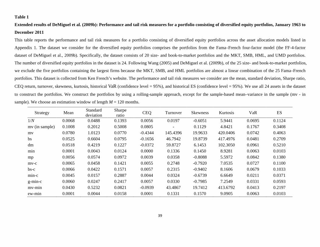
Table 1 reports the performance and tail risk measures for a portfolio consisting of
diversified equity portfolios across the asset allocation models considered by DeMiguel et al.
(2009b). The asset allocation models are listed in Appendix 1.
whose sample period includes the recent US subprime crisis. Section 4.2 reports the
empirical results using individual stocks.
4.1 Results from the analysis of diversified equity portfolios
4.1.1 Performance and tail risk measures
[Insert Table 1 about here]
12
11 The sample period of DeMiguel et al. (2009b) is from July 1963 to November 2004. 12 We construct portfolios by using a rolling-sample approach, except for the sample-based mean–variance in sample (mv - in sample).

14
Analyzing the performance measures, we find several results that are consistent with
those of DeMiguel et al. (2009b). First, none of the strategies from the optimizing models
consistently outperform the 1/N strategy. While the constrained strategies have higher Sharpe
ratios than the 1/N strategy, none of the strategies from the optimal models is better than the 1/N
strategy in terms of CEQ and turnover. In particular, the sample-based mean–variance strategy
(mv) is worse than the 1/N strategy. In Table 1, while the Sharpe ratio, CEQ, and turnover of the
1/N strategy are 0.1393, 0.0056, and 0.0197, respectively, those of the sample-based mean–
variance strategy (mv) are 0.0770, -0.4344, and 145.4396, respectively. Second, Bayesian
strategies seem to improve performance, but not very effectively. While the Bayes–Stein strategy
(bs) and the Bayesian data-and-model strategy (dm) outperform the sample-based mean–variance
strategy (mv), the 1/N strategy outperforms these Bayesian strategies. Third, constrained policies
help improve performance, but not sufficiently. Constrained strategies do better than their
corresponding unconstrained strategies. For example, while the Sharpe ratio, CEQ, and turnover
of the Bayes–Stein strategy (bs) are 0.0795, -0.1656, and 46.7942, respectively, those of the
Bayes–Stein strategy with short sale constraints (bs-c) are 0.1571, 0.0057, and 0.2315,
respectively. However, the constrained strategies do not consistently outperform the 1/N strategy.
Although some of the constrained strategies, such as the minimum-variance strategy with short
sale constraints (min-c) and minimum-variance with generalized constraints (g-min-c), have
significantly higher Sharpe ratios than the 1/N strategy, none of the constrained strategies has a
higher CEQ than the 1/N strategy in a statistically significant way. Furthermore, the 1/N strategy
has the lowest turnover.
From analysis of the tail risk measures, first, we find that the strategy that exhibits better
performance tends to have negative skewness and positive kurtosis. In particular, the skewness of

15
the 1/N strategy and the constrained strategies, which outperform the other strategies, is less than
-0.6 and the kurtosis of those strategies is greater than five. This result implies that the better –
performing strategy tends to increase tail risk exposure. Second, the strategy that contains
outliers from extreme portfolio weights tends to have extremely large skewness and kurtosis.
For example, the skewness of the sample-based mean–variance strategy (mv) and the Bayes–
Stein strategy (bs) is greater than 19 and their kurtosis is greater than 400. Third, the strategy that
has a lower standard deviation tends to have lower VaR and ES. Specifically, the minimum-
variance strategy (min) and the mixture of minimum-variance and 1/N strategies (ew-min) have
the lowest VaR and ES values, as well as standard deviation.
4.1.2 Return distribution
To illustrate the difference in tail risk exposure across strategies, we compare the return
distributions of the naive 1/N and optimal portfolio strategies.
[Insert Figure 1 about here]
Figure 1 reports the kernel smoothed histogram for the return distributions of portfolios
consisting of both diversified stock portfolios from the naive 1/N strategy as well as optimal
portfolio strategies. To simplify the graph, we consider only the sample-based mean–variance
(mv) and the sample-based mean–variance with short sale constraints (mv-c) as the optimal
portfolio strategy. To compare these return distributions to a normal distribution, in Figure 1 we
also report the corresponding normal distribution generated by the pooled mean and pooled
standard deviation from the return distributions of the naive 1/N and optimal portfolio strategies.

16
Figure 1 shows that all strategies exhibit leptokurtic distribution, which means positive
excess kurtosis and heavier tails than the normal distribution. However, only the strategies that
have better performance, the naive 1/N strategy and the sample-based mean–variance portfolio
strategy with short sale constraints (mv-c), have negatively skewed distribution, which means a
larger and longer left tail than the normal distribution. In other words, the strategy that has better
performance tends to have increased left tail risk exposure and reduced upside potential. This
tendency is clearer in the naive 1/N strategy than in the other strategies. This result implies that
the strategy that has better performance, especially the naive 1/N strategy, may have a more
concave payoff than the strategy with poor performance.
4.1.3 Concavity of the portfolio payoff
In this section, we examine whether the portfolio from the naive 1/N strategy or the
optimal portfolio strategies has concave payoff relative to the equity benchmark. More
specifically, to examine the concavity of a portfolio’s payoff, we use the coefficients of
Henriksson and Merton (1981) and Treynor and Mazuy (1966). Henriksson and Merton (1981)
and Treynor and Mazuy (1966) propose a test of market timing ability in an extended market
model regression since they argue that a fund manager who can successfully time the market
should demonstrate convex returns relative to a benchmark. However, nonlinear return patterns
are not limited to market timing strategies. For example, Agarwal and Naik (2004) argue that
concave payoff patterns in hedge fund returns result from exposure to option-based risk factors
rather than to negative timing ability. While intent to limit tail risk exposure through portfolio
insurance–type strategies will lead to convex returns relative to a benchmark, increases in tail
risk exposure will lead to concave returns.

17
The coefficients of Henriksson and Merton (1981) and Treynor and Mazuy (1966) are
computed from the regression
0 1 2 ,t t t tr m cγ γ γ ε= + + + (13)
where rt and mt
( ,0)t tc Max m= −
are the excess returns on the portfolio and the market, respectively. The timing
variable is for Henriksson and Merton (1981) and 2t tc m= for Treynor and
Mazuy (1966).
[Insert Table 2 about here]
Table 2 reports the timing coefficients for a portfolio consisting of diversified equity
portfolios across the asset allocation models listed in Appendix 1. The t-statistics are given in
parentheses. Numbers in bold denote the coefficients’ statistical significance. In Table 2, we find
that the strategies that show higher performance in Table 1—such as the naive 1/N strategy,
MacKinlay and Pastor’s (2000) missing-factor model (mp), the sample-based mean–variance
with short sale constraints (mv-c), the Bayes–Stein strategy with short sale constraints (bs-c), and
the minimum-variance strategy with generalized constraints (g-min-c)—have a concave payoff
relative to the equity benchmark. In particular, these strategies have a significantly positive
coefficient for the market portfolio ( 1γ ) and a significantly negative coefficient for the timing
variable ( 2γ ). On the other hand, the strategies that show lower performance in Table 1—such as
the sample-based mean–variance (mv) and the Bayes–Stein (bs)—seem to have a convex payoff
rather than a concave payoff.
In summary, we find that none of the strategies from the optimizing models consistently
outperforms the naive 1/N strategy in the analysis of diversified equity portfolios. A high-
18
performance strategy tends to have increased left tail risk exposure, reduced upside potential, and
a concave payoff relative to the equity benchmark. This tendency is clearer in the naive 1/N
strategy than in the optimal portfolio strategies.
4.2 Results from the analysis of individual stock portfolios
4.2.1 Performance and tail risk measures
[Insert Figure 2 about here]
In this section, we use individual stocks to construct portfolios while we use diversified
equity portfolios to construct the portfolios in Section 4.1. Figure 2 shows the mean value of the
performance and tail risk measures for the naive 1/N portfolio, the sample-based mean–variance
portfolio, and the sample-based mean–variance portfolio with short sale constraints. 13
Analyzing the performance measures, we find several results that are consistent with the
literature on optimal portfolio choice in the presence of estimation error. First, we find that the
naive diversification strategy consistently outperforms the optimal diversification strategies.
Regardless of the kind of performance measure or the number of stocks in a portfolio, the naive
To
investigate not only the comparison between naive and optimal diversification in terms of
performance and tail risk but also the effect of diversification on performance and tail risk, we
plot the performance and tail risk measures as a function of the number of stocks in a portfolio.
In addition to the mean value of measures, the dotted line in Figure 2 shows the confidence band
of each measure. The range of the confidence band is between -2 and 2 standard deviations.
13 Appendix 2 reports the tables for the mean values of these measures.

19
1/N portfolio has a higher Sharpe ratio, CEQ return, MPPM, and lower turnover than the mean–
variance portfolios. In particular, in the case of N = 30, the Sharpe ratio of the naive 1/N portfolio
is 0.1921, while those for the sample-based mean–variance portfolio and the sample-based
mean–variance portfolio with short sale constraints are -0.0079 and 0.0717, respectively. The
CEQ return of the naive 1/N portfolio is 0.0079, but those of the sample-based mean–variance
portfolio and the sample-based mean–variance portfolio with short sale constraints are
only -2.9122 and 0.0024, respectively. The sample-based mean–variance portfolio has an
extremely large turnover of 24.6812 compared to 0.0686 for the naive 1/N portfolio. Last, only
the naive 1/N strategy has a positive value of MPPM (0.0640), while the other optimal strategies
have a negative value of MPPM (-4.3921 for the sample-based mean–variance portfolio and -
0.0791 for the sample-based mean–variance portfolio with short sale constraints).
Second, the short sale constraints improve performance, but not sufficiently. The sample-
based mean–variance portfolio with short sale constraints consistently outperforms that without
constraints. The short sale constraints seem to help reduce extreme weights that fluctuate
substantially over time to a certain degree. However, the sample-based mean–variance portfolio
with short sale constraints still underperforms the naive 1/N portfolio.
Third, the magnitude of the difference between the performance measures for the naive
1/N strategy and for the optimal portfolio strategies increases as the number of stocks in the
portfolios increases. For example, in the case of N = 10, the differences in the Sharpe ratio, CEQ
return, turnover, and MPPM between the naive 1/N strategy and the sample-based mean–
variance portfolio are 0.1288, 1.1876, -8.3135, and 2.9902, respectively. As the number of stocks
in the portfolios increases to N = 40, the differences also increase to 0.2135, 3.9855, -33.9899,
and 5.0607, respectively. Especially for the sample-based mean–variance portfolio, the standard

20
deviation of the portfolio return is an increasing function of the number of stocks in the portfolio,
although it should be a decreasing function if it is a truly optimal portfolio. As DeMiguel et al.
(2009b) point out, the larger number of stocks implies more parameters to be estimated and,
therefore, more room for estimation error. Moreover, all other things being equal, the larger
number of stocks in a portfolio makes naive diversification more effective relative to optimal
diversification.
From analyzing tail risk measures, first, we find that the skewness for the naive 1/N
strategy is more negative than that for the optimal portfolio strategies. In particular, in the case of
N = 30, the skewness measure for the naive 1/N portfolio is -0.6108, while those for the sample-
based mean–variance portfolio and the sample-based mean–variance portfolio with short sale
constraints are -0.4804 and 0.0628, respectively. Moreover, as the number of stocks in the
portfolios increases, the skewness for the naive 1/N portfolio decreases than the mean–variance
portfolios. For example, the change in skewness from the naive 1/N portfolios with N = 10 to
those with N = 40 is -0.4490, while those for the sample-based mean–variance portfolio and the
sample-based mean–variance portfolio with short sale constraints are -0.2636 and -0.0305,
respectively. This tendency in skewness for the naive 1/N portfolio implies that naive
diversification increases tail risk.
Second, the kurtosis for the naive 1/N strategy is more positive than for the sample-based
mean–variance portfolio with short sale constraints. Although the sample-based mean–variance
portfolio has the largest value of the kurtosis among the strategies we consider, this is largely due
to outliers resulting from extreme portfolio weights. Furthermore, we find that the kurtosis for
the naive 1/N strategy is an increasing function of the number of stocks in the portfolios while
that for the sample-based mean–variance portfolio with short sale constraints is a decreasing

21
function of the number of portfolio stocks. Similar to the skewness results, this tendency in the
kurtosis of the naive 1/N portfolio implies that naive diversification increases tail risk.
Third, the values of VaR and ES for the optimal portfolio strategies are higher than for the
naive 1/N strategy. Moreover, while the VaR and ES for the sample-based mean–variance
portfolio are increasing functions of the number of portfolio stocks, these measures for the naive
1/N portfolio are decreasing functions of the number of portfolio stocks. As for the results from
the standard deviation (Panel B in Figure 2), this is due to the extreme weights that fluctuate
substantially over time due to the estimation error of the optimal portfolio strategy.
4.2.2 Return distribution
[Insert Figure 3 about here]
Figure 3 shows the kernel smoothed histogram for the return distributions of portfolios
consisting of randomly selected stocks from the naive 1/N strategy as well as the optimal
portfolio strategies with N = 5 and N = 50. We normalize the portfolio return by using the mean
and standard deviation of each portfolio. For this reason, the x-axis in Figure 3 is the mean
deviation normalized by the standard deviation. From this normalization, we obtain 1,200,000
returns (120ⅹ10,000) for each strategy. Figure 3 also reports the corresponding normal
distribution generated by the pooled mean and pooled standard deviation from the normalized
return distributions of the naive 1/N and optimal portfolio strategies.
Consistent with the results in Section 4.2.1, for both N = 5 and N = 50 Figure 3 shows
that all strategies exhibit leptokurtic distribution, which means positive excess kurtosis and
22
heavier tails than the normal distribution. However, the naive 1/N strategy has a more negatively
skewed distribution than the optimal portfolio strategies. This means that the naive 1/N strategy
has a larger and longer left tail distribution than the optimal portfolio strategies. In other words,
the naive 1/N strategy tends to increase in left tail risk exposure and reduce upside potential.
Moreover, this tendency gets stronger as the number of portfolio stocks increases. This result
implies that the naive 1/N strategy may have a more concave payoff than the optimal portfolio
strategies.
4.2.3 Concavity of portfolio payoff
[Insert Figure 4 about here]
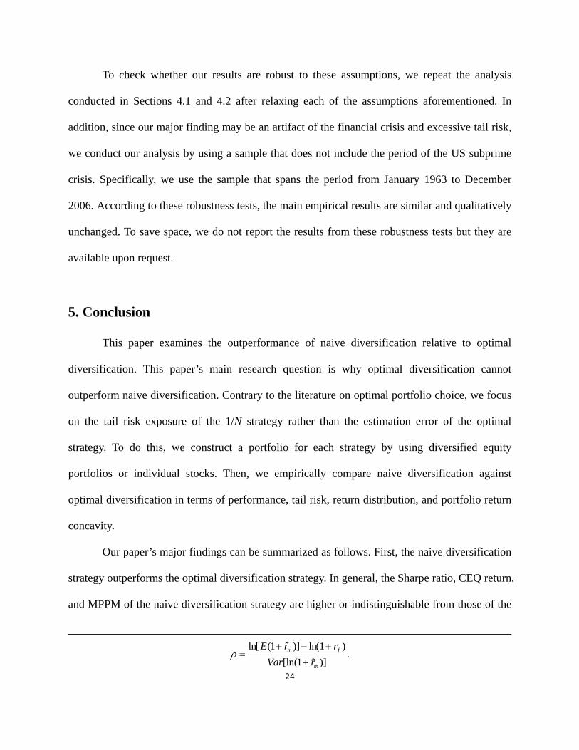
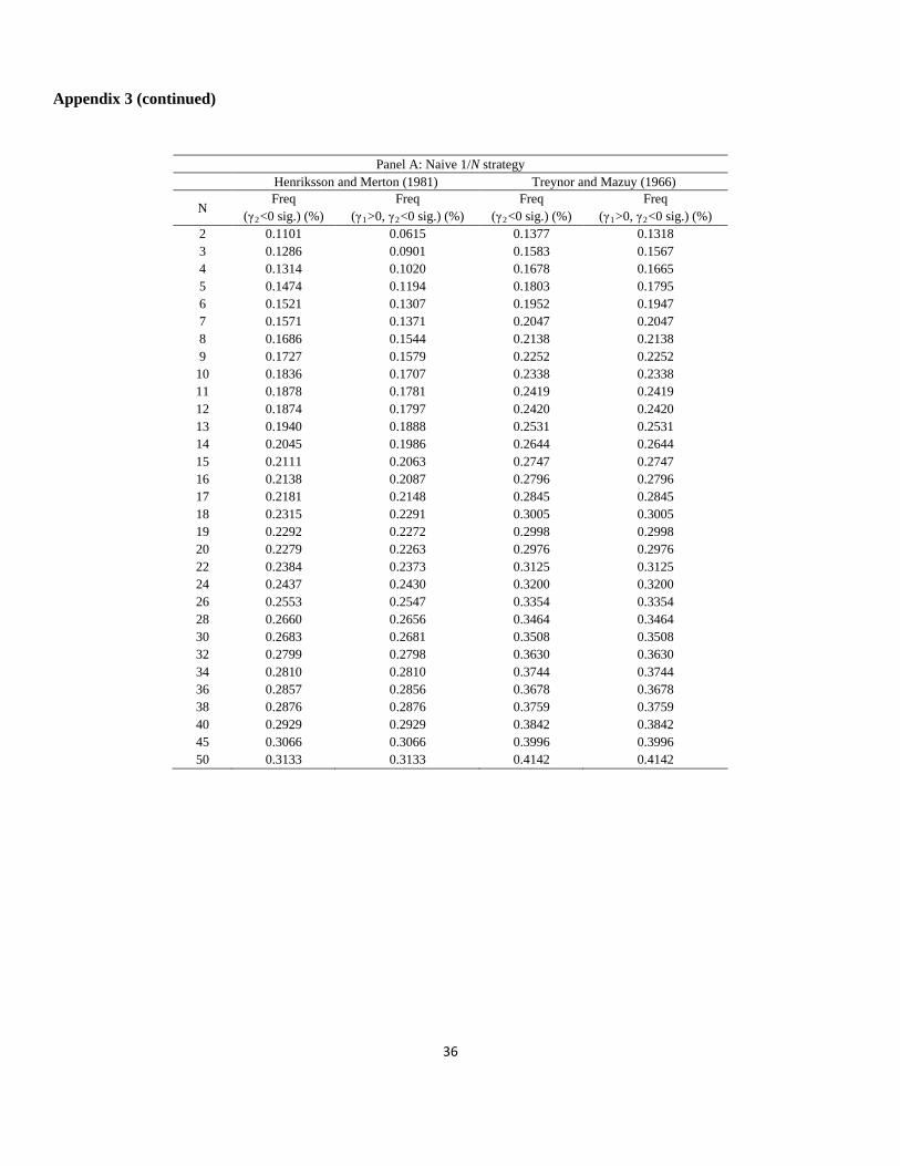
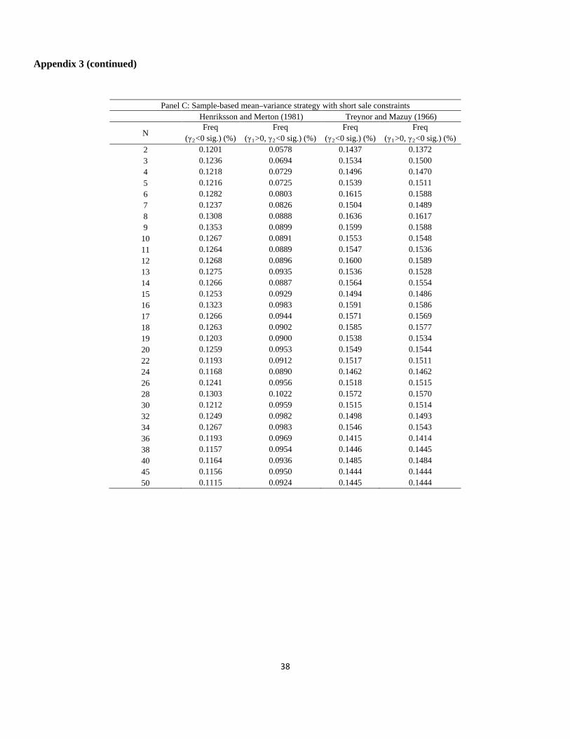
Figure 4 presents the fraction of times that the portfolio exhibits a concave payoff.14
2 0γ <
Panels A and B report the results for Henriksson and Merton (1981) and Treynor and Mazuy
(1966), respectively. In each panel, the upper figure shows the fraction of times the portfolio
showed a significant at the 5% level. The lower figure shows the fraction of times the
portfolio showed a significant 1 0γ > and 2 0γ < at the 5% level. From the results of Henriksson
and Merton (1981) and of Treynor and Mazuy (1966), we find that the fraction of times the
portfolio exhibits a concave payoff in the naive 1/N strategy is much higher than for the optimal
portfolio strategies. In particular, in the case of N = 30, from the results for Treynor and Mazuy
(1966), 35.1% of the naive 1/N portfolio shows a concave payoff relative to the equity
benchmark, while only 5.3% of the sample-based mean–variance portfolio and 15.1% of the 14 Appendix 3 reports the tables for the fraction of times the portfolio exhibits a concave payoff.

23
sample-based mean–variance portfolio with short sale constraints show a concave payoff.
Moreover, the fraction of times the portfolio shows a concave payoff in the naive 1/N strategy
increases as the number of portfolio stocks increases. This implies that the 1/N diversification
increases the concavity of the portfolio’s payoff.
To summarize the results in Sections 4.1 and 4.2, using individual stocks as well as
diversified equity portfolios, we find that the naive diversification strategy consistently
outperforms optimal diversification strategies. In addition, naive diversification increases tail risk
and makes portfolio returns more concave relative to an equity benchmark. Last, the tendency
toward naive diversification increases as the number of portfolio stocks increases. Therefore, the
outperformance of naive diversification relative to optimal diversification results from
compensation for the increase in tail risk and the reduced upside potential associated with a
concave payoff.
4.3 Results from robustness tests
In the benchmark case reported in Sections 4.1 and 4.2, we assume the following: (i) The
length of the estimation window is M = 120 months, rather than M = {60, 180}; (ii) the holding
period is one month rather than one year; (iii) the portfolio evaluated consists of only risky assets
rather than also including risk-free assets; (iv) the 1/N-with-rebalancing strategy is used rather
than the 1/N-buy-and-hold strategy; (v) in calculating CEQ, the investor has a risk aversion of
1γ = rather than some other value, say {3,5,10}γ = ; and (vi) in calculating the MPPM, the
investor has a risk aversion of 3ρ = rather than the value estimated from the market portfolio.15
15 If the market portfolio has a lognormal return, 1+rm, then the risk aversion parameter ρ can be selected so that
24
To check whether our results are robust to these assumptions, we repeat the analysis
conducted in Sections 4.1 and 4.2 after relaxing each of the assumptions aforementioned. In
addition, since our major finding may be an artifact of the financial crisis and excessive tail risk,
we conduct our analysis by using a sample that does not include the period of the US subprime
crisis. Specifically, we use the sample that spans the period from January 1963 to December
2006. According to these robustness tests, the main empirical results are similar and qualitatively
unchanged. To save space, we do not report the results from these robustness tests but they are
available upon request.
5. Conclusion
This paper examines the outperformance of naive diversification relative to optimal
diversification. This paper’s main research question is why optimal diversification cannot
outperform naive diversification. Contrary to the literature on optimal portfolio choice, we focus
on the tail risk exposure of the 1/N strategy rather than the estimation error of the optimal
strategy. To do this, we construct a portfolio for each strategy by using diversified equity
portfolios or individual stocks. Then, we empirically compare naive diversification against
optimal diversification in terms of performance, tail risk, return distribution, and portfolio return
concavity.
Our paper’s major findings can be summarized as follows. First, the naive diversification
strategy outperforms the optimal diversification strategy. In general, the Sharpe ratio, CEQ return,
and MPPM of the naive diversification strategy are higher or indistinguishable from those of the
ln[ (1 )] ln(1 )
.[ln(1 )]
m f
m
E r rVar r
ρ+ − +
=+

25
optimal diversification strategy. Moreover, the naive diversification strategy has the lowest
turnover. Second, naive diversification increases left tail risk exposure. The naive 1/N portfolio
tends not only to have negative skewness and positive excess kurtosis but also to diminish the
upside return potential. Third, naive diversification makes the portfolio returns more concave
relative to the equity benchmark. From the test of Henriksson and Merton (1981) and Treynor
and Mazuy (1966), we find that the portfolio return from naive diversification exhibits a much
more concave payoff pattern than the optimal diversification. Fourth, these tendencies of naive
diversification get stronger as the number of portfolio stocks increases.
We do not want to imply that naive diversification is a generally recommendable
investment strategy. Instead, we imply that the outperformance of naive diversification relative to
optimal diversification can be explained as due to compensation for the increase in tail risk and
the reduced upside potential associated with a concave payoff. In addition, this paper suggests
that to evaluate the performance of a particular asset allocation strategy, tail risk exposure should
be taken into account in addition to portfolio risk.
26
References
Agarwal, V., Naik, N., 2004. Risks and portfolio decisions involving hedge funds. Review of Financial Studies 17, 63–98.
Bawa, V. S., Brown, S. J., Klein, R., 1979. Estimation Risk and Optimal Portfolio Choice. Amsterdam: North Holland.
Behr, P., Guettler, A., Truebenbach, F., 2012. Using industry momentum to improve portfolio performance, Journal of Banking and Finance 36, 1414–1423.
Benartzi, S., Thaler, R., 2001. Naive diversification strategies in defined contribution saving plan. American Economic Review 91, 79–98.
Best, M. J., Grauer, R. R., 1992. Positively weighted minimum-variance portfolios and the structure of asset expected returns. Journal of Financial and Quantitative Analysis 27, 513–537.
Bloomfield, T., Leftwich, R., Long, J., 1977. Portfolio strategies and performance. Journal of Financial Economics 5, 201–218.
Brandt, M. W., 2010. Portfolio choice problems, in Y. Ait-Sahalia and L.P. Hansen (eds.), Handbook of Financial Econometrics, Volume 1: Tools and Techniques. Amsterdam: North Holland, 269–336.
Brown, S. J., Gallagher, D. R., Steenbeek, O. W., Swan, P. L., 2006. Concave payoff patterns in equity fund holdings and transactions. Working paper, New York University.
Brown, S. J., Gregoriou, G. N., Pascalau, R., 2012. Diversification in funds of hedge funds: Is it possible to overdiversify? Review of Asset Pricing Studies 2, 89–110.

27
Campbell, J. Y., Viceira, L. M., 2002. Strategic Asset Allocation. New York: Oxford University Press.
DeMiguel, V., Garlappi, L., Nogales, F. J., Uppal, R., 2009a. A generalized approach to portfolio optimization: Improving performance by constraining portfolio norms. Management Science 55, 798–812.
DeMiguel, V., Garlappi, L., Uppal, R., 2009b. Optimal versus naive diversification: How inefficient is the 1/N portfolio strategy? Review of Financial Studies 22, 1915–1953.
Garlappi, L., Uppal, R., Wang, T., 2007. Portfolio selection with parameter and model uncertainty: A multi-prior approach. Review of Financial Studies 20, 41–81.
Goetzmann, W., Ingersoll, J., Spiegel, M., Welch, I., 2007. Portfolio performance manipulation and manipulation-proof performance measures. Review of Financial Studies 20, 1503–1546.
Green, R., Hollifield, B., 1992. When will mean–variance efficient portfolios be well diversified? Journal of Finance 47, 1785–1809.
Grinold, R. C., Kahn, R. N., 1999. Active Portfolio Management: Quantitative Theory and Applications. New York: McGraw-Hill.
Henriksson, R. D., Merton, R. C., 1981. On market timing and investment performance. II. Statistical procedures for evaluating forecasting skills. Journal of Business 54, 513–533.
Huberman, G., Jiang, W., 2006. Offering versus choice in 401(k) plans: Equity exposure and number of funds. Journal of Finance 61, 763–801.
28
Jagannathan, R., Ma, T., 2003. Risk reduction in large portfolios: Why imposing the wrong constraints helps. Journal of Finance 58, 1651–1684.
Jorion, P., 1986. Bayes–Stein estimation for portfolio analysis. Journal of Financial and Quantitative Analysis 21, 279–292.
Jorion, P., 1991. Bayesian and CAPM estimators of the means: Implications for portfolio selection. Journal of Banking and Finance 15, 717–727.
Kan, R., Zhou, G., 2007. Optimal portfolio choice with parameter uncertainty. Journal of Financial and Quantitative Analysis 42, 621–656.
Kourtis, A., Dotsis, G., Markellos, R. N., 2012. Parameter uncertainty in portfolio selection: Shrinking the inverse covariance matrix. Journal of Banking and Finance 36, 2522–2531.
Liang, N., Weisbenner, S., 2002. Investor behavior and the purchase of company stock in 401(k) plans—The importance of plan design. Working paper, Board of Governors of the Federal Reserve System and University of Illinois.
Litterman, B., 2003. Modern Investment Management: An Equilibrium Approach. New York: Wiley.
MacKinlay, A.C., Pastor, L., 2000. Asset pricing models: Implications for expected returns and portfolio selection. Review of Financial Studies 13, 883–916.
Markowitz, H. M., 1952. Mean–variance analysis in portfolio choice and capital markets. Journal of Finance 7, 77–91.
29
Markowitz, H.M., 1959. Portfolio Selection. New York: Wiley.
Merton, R. C., 1980. On estimating the expected return on the market: An exploratory investigation. Journal of Financial Economics 8, 323–361.
Meucci, A., 2005. Risk and Asset Allocation. New York: Springer-Verlag.
Pastor, L., 2000. Portfolio selection and asset pricing models. Journal of Finance 55, 179–223.
Pflug, G. C., Pichler, A., Wozabal, D., 2012. The 1/N investment strategy is optimal under high model ambiguity. Journal of Banking and Finance 36, 410–417.
Sharpe, W. F., 1970. Portfolio Theory and Capital Markets. New York: McGraw-Hill.
Treynor, J., Mazuy, K., 1966. Can mutual funds outguess the market? Harvard Business Review 44, 131–136.
Tu, J., Zhou, G., 2011. Markowitz meets Talmud: A combination of sophisticated and naive diversification strategies. Journal of Financial Economics 99, 204–215.
Wang, Z., 2005. A shrinkage approach to model uncertainty and asset allocation. Review of Financial Studies 18, 673–705.

30
Appendix 1
List of various asset allocation models considered by DeMiguel et al. (2009b)
This table lists the various asset allocation models considered by DeMiguel et al. (2009b). The last
column of the table gives the abbreviation used to refer to the strategy in Tables 1 and 2.
# Model Abbreviation Naive 1 Naive 1/N 1/N Classical approach 2 Sample-based mean–variance in sample mv (in sample) 3 Sample-based mean–variance mv Bayesian approach 4 Bayes–Stein bs 5 Bayesian data-and-model dm Moment restrictions 6 Minimum variance min 7 MacKinlay and Pastor’s (2000) missing-factor model mp Portfolio constraints 8 Sample-based mean–variance with short sale constraints mv-c 9 Bayes–Stein with short sale constraints bs-c 10 Minimum-variance with short sale constraints min-c 11 Minimum-variance with generalized constraints g-min-c Optimal combinations of portfolios 12 Kan and Zhou’s (2007) “three-fund” model mv-min 13 Mixture of minimum variance and 1/N ew-min
31
Appendix 2
Performance and tail risk measures for a portfolio consisting of randomly selected stocks, January 1963 to
December 2011
This table reports the mean value of the performance and tail risk measures for portfolios consisting of randomly selected
stocks from the naive 1/N and optimal portfolio strategies. Panels A to C report the results for the naive 1/N strategy, the
sample-based mean–variance strategy, and the sample-based mean–variance strategy with short sale constraints,
respectively. The performance and tail risk measures we consider are the mean, standard deviation, Sharpe ratio, CEQ
return, turnover, MPPM (ρ = 3), skewness, kurtosis, historical VaR (confidence level = 95%), and historical ES
(confidence level = 95%). The number of portfolio stocks, N, ranges from two to 50. For each N, N stocks are randomly
selected B times to construct portfolios (in our study, B = 10,000). To obtain sensible measures of performance and tail
risk for the portfolios from the time-series regressions, we require that all N stocks that are randomly selected to construct
portfolios have at least 120 months of overlapping return history. We construct portfolios by using a rolling-sample
approach. We choose an estimation window of length M = 120 months. To avoid oversampling returns in the period of the
US subprime crisis, we generate the first 120 months of portfolio returns.
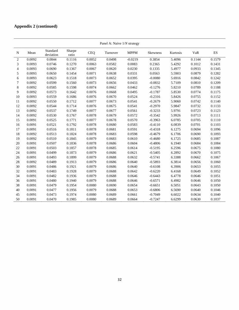
32
Appendix 2 (continued)
Panel A: Naive 1/N strategy
N Mean Standard deviation
Sharpe ratio CEQ Turnover MPPM Skewness Kurtosis VaR ES
2 0.0092 0.0844 0.1116 0.0052 0.0498 -0.0219 0.3854 5.4096 0.1144 0.1579 3 0.0093 0.0746 0.1270 0.0063 0.0582 0.0083 0.2365 5.4292 0.1012 0.1431 4 0.0093 0.0690 0.1367 0.0067 0.0620 0.0230 0.1335 5.4977 0.0933 0.1345 5 0.0093 0.0650 0.1454 0.0071 0.0638 0.0331 0.0563 5.5903 0.0879 0.1282 6 0.0093 0.0623 0.1518 0.0073 0.0652 0.0395 -0.0080 5.6916 0.0842 0.1242 7 0.0092 0.0599 0.1560 0.0073 0.0656 0.0433 -0.0832 5.7109 0.0810 0.1209 8 0.0092 0.0585 0.1598 0.0074 0.0662 0.0462 -0.1276 5.8210 0.0789 0.1188 9 0.0092 0.0573 0.1642 0.0076 0.0668 0.0495 -0.1787 5.8530 0.0774 0.1175
10 0.0093 0.0559 0.1686 0.0076 0.0670 0.0524 -0.2316 5.8426 0.0755 0.1152 11 0.0092 0.0550 0.1712 0.0077 0.0673 0.0541 -0.2679 5.9060 0.0742 0.1140 12 0.0092 0.0544 0.1714 0.0076 0.0675 0.0541 -0.2970 5.9847 0.0732 0.1133 13 0.0092 0.0537 0.1749 0.0077 0.0677 0.0561 -0.3233 5.9791 0.0723 0.1123 14 0.0092 0.0530 0.1767 0.0078 0.0679 0.0572 -0.3542 5.9926 0.0713 0.1111 15 0.0091 0.0525 0.1771 0.0077 0.0678 0.0570 -0.3963 6.0785 0.0705 0.1110 16 0.0091 0.0521 0.1792 0.0078 0.0680 0.0583 -0.4110 6.0839 0.0701 0.1103 17 0.0091 0.0516 0.1811 0.0078 0.0681 0.0591 -0.4318 6.1275 0.0694 0.1096 18 0.0092 0.0513 0.1824 0.0078 0.0683 0.0598 -0.4679 6.1706 0.0690 0.1093 19 0.0092 0.0510 0.1845 0.0079 0.0683 0.0610 -0.4680 6.1725 0.0685 0.1087 20 0.0091 0.0507 0.1836 0.0078 0.0686 0.0604 -0.4806 6.1940 0.0684 0.1084 22 0.0091 0.0503 0.1857 0.0078 0.0685 0.0614 -0.5195 6.2596 0.0675 0.1080 24 0.0091 0.0499 0.1873 0.0079 0.0686 0.0621 -0.5405 6.2892 0.0670 0.1075 26 0.0091 0.0493 0.1899 0.0079 0.0688 0.0632 -0.5741 6.3388 0.0662 0.1067 28 0.0092 0.0489 0.1913 0.0079 0.0686 0.0640 -0.5893 6.3814 0.0656 0.1060 30 0.0091 0.0486 0.1921 0.0079 0.0686 0.0640 -0.6108 6.3906 0.0653 0.1055 32 0.0091 0.0483 0.1928 0.0079 0.0688 0.0642 -0.6220 6.4168 0.0649 0.1052 34 0.0091 0.0482 0.1936 0.0079 0.0688 0.0646 -0.6443 6.4778 0.0646 0.1051 36 0.0091 0.0480 0.1940 0.0079 0.0688 0.0646 -0.6571 6.4982 0.0646 0.1050 38 0.0091 0.0479 0.1954 0.0080 0.0690 0.0654 -0.6651 6.5051 0.0643 0.1050 40 0.0091 0.0477 0.1956 0.0079 0.0688 0.0653 -0.6806 6.5690 0.0640 0.1046 45 0.0091 0.0473 0.1974 0.0080 0.0689 0.0661 -0.7049 6.6022 0.0634 0.1040 50 0.0091 0.0470 0.1985 0.0080 0.0689 0.0664 -0.7247 6.6299 0.0630 0.1037
33
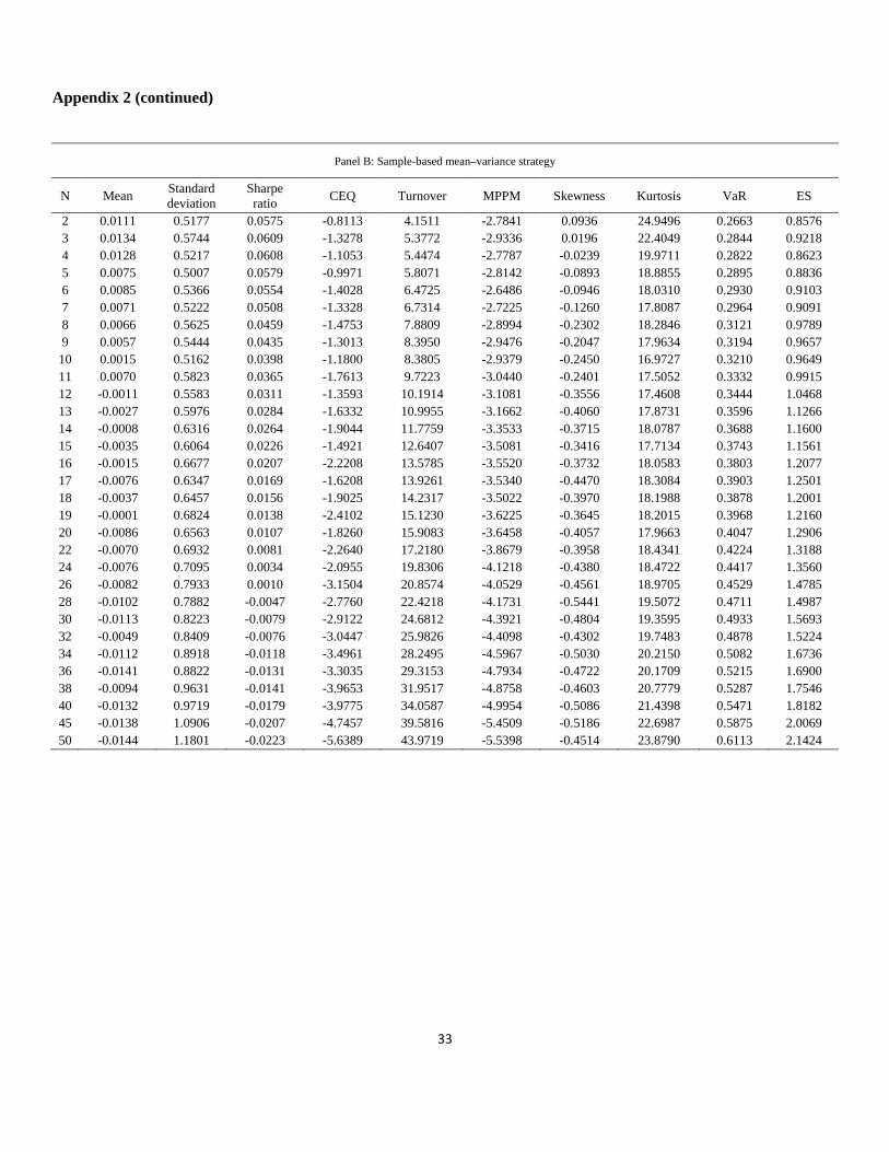
Appendix 2 (continued)
Panel B: Sample-based mean–variance strategy
N Mean Standard deviation
Sharpe ratio CEQ Turnover MPPM Skewness Kurtosis VaR ES
2 0.0111 0.5177 0.0575 -0.8113 4.1511 -2.7841 0.0936 24.9496 0.2663 0.8576 3 0.0134 0.5744 0.0609 -1.3278 5.3772 -2.9336 0.0196 22.4049 0.2844 0.9218 4 0.0128 0.5217 0.0608 -1.1053 5.4474 -2.7787 -0.0239 19.9711 0.2822 0.8623 5 0.0075 0.5007 0.0579 -0.9971 5.8071 -2.8142 -0.0893 18.8855 0.2895 0.8836 6 0.0085 0.5366 0.0554 -1.4028 6.4725 -2.6486 -0.0946 18.0310 0.2930 0.9103 7 0.0071 0.5222 0.0508 -1.3328 6.7314 -2.7225 -0.1260 17.8087 0.2964 0.9091 8 0.0066 0.5625 0.0459 -1.4753 7.8809 -2.8994 -0.2302 18.2846 0.3121 0.9789 9 0.0057 0.5444 0.0435 -1.3013 8.3950 -2.9476 -0.2047 17.9634 0.3194 0.9657
10 0.0015 0.5162 0.0398 -1.1800 8.3805 -2.9379 -0.2450 16.9727 0.3210 0.9649 11 0.0070 0.5823 0.0365 -1.7613 9.7223 -3.0440 -0.2401 17.5052 0.3332 0.9915 12 -0.0011 0.5583 0.0311 -1.3593 10.1914 -3.1081 -0.3556 17.4608 0.3444 1.0468 13 -0.0027 0.5976 0.0284 -1.6332 10.9955 -3.1662 -0.4060 17.8731 0.3596 1.1266 14 -0.0008 0.6316 0.0264 -1.9044 11.7759 -3.3533 -0.3715 18.0787 0.3688 1.1600 15 -0.0035 0.6064 0.0226 -1.4921 12.6407 -3.5081 -0.3416 17.7134 0.3743 1.1561 16 -0.0015 0.6677 0.0207 -2.2208 13.5785 -3.5520 -0.3732 18.0583 0.3803 1.2077 17 -0.0076 0.6347 0.0169 -1.6208 13.9261 -3.5340 -0.4470 18.3084 0.3903 1.2501 18 -0.0037 0.6457 0.0156 -1.9025 14.2317 -3.5022 -0.3970 18.1988 0.3878 1.2001 19 -0.0001 0.6824 0.0138 -2.4102 15.1230 -3.6225 -0.3645 18.2015 0.3968 1.2160 20 -0.0086 0.6563 0.0107 -1.8260 15.9083 -3.6458 -0.4057 17.9663 0.4047 1.2906 22 -0.0070 0.6932 0.0081 -2.2640 17.2180 -3.8679 -0.3958 18.4341 0.4224 1.3188 24 -0.0076 0.7095 0.0034 -2.0955 19.8306 -4.1218 -0.4380 18.4722 0.4417 1.3560 26 -0.0082 0.7933 0.0010 -3.1504 20.8574 -4.0529 -0.4561 18.9705 0.4529 1.4785 28 -0.0102 0.7882 -0.0047 -2.7760 22.4218 -4.1731 -0.5441 19.5072 0.4711 1.4987 30 -0.0113 0.8223 -0.0079 -2.9122 24.6812 -4.3921 -0.4804 19.3595 0.4933 1.5693 32 -0.0049 0.8409 -0.0076 -3.0447 25.9826 -4.4098 -0.4302 19.7483 0.4878 1.5224 34 -0.0112 0.8918 -0.0118 -3.4961 28.2495 -4.5967 -0.5030 20.2150 0.5082 1.6736 36 -0.0141 0.8822 -0.0131 -3.3035 29.3153 -4.7934 -0.4722 20.1709 0.5215 1.6900 38 -0.0094 0.9631 -0.0141 -3.9653 31.9517 -4.8758 -0.4603 20.7779 0.5287 1.7546 40 -0.0132 0.9719 -0.0179 -3.9775 34.0587 -4.9954 -0.5086 21.4398 0.5471 1.8182 45 -0.0138 1.0906 -0.0207 -4.7457 39.5816 -5.4509 -0.5186 22.6987 0.5875 2.0069 50 -0.0144 1.1801 -0.0223 -5.6389 43.9719 -5.5398 -0.4514 23.8790 0.6113 2.1424
34
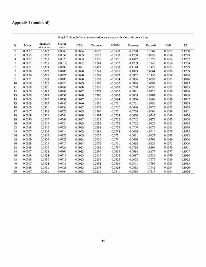
Appendix 2 (continued)
Panel C: Sample-based mean–variance strategy with short sale constraints
N Mean Standard deviation
Sharpe ratio CEQ Turnover MPPM Skewness Kurtosis VaR ES
2 0.0077 0.0892 0.0863 0.0034 0.0678 -0.0590 0.2728 5.1567 0.1273 0.1758 3 0.0075 0.0868 0.0854 0.0035 0.1017 -0.0538 0.1700 5.0858 0.1256 0.1749 4 0.0073 0.0868 0.0826 0.0033 0.1220 -0.0561 0.1477 5.1372 0.1264 0.1762 5 0.0071 0.0865 0.0812 0.0032 0.1361 -0.0562 0.1289 5.1240 0.1266 0.1764 6 0.0071 0.0869 0.0793 0.0031 0.1472 -0.0588 0.1148 5.1429 0.1273 0.1779 7 0.0070 0.0872 0.0785 0.0030 0.1541 -0.0606 0.1023 5.0661 0.1279 0.1789 8 0.0070 0.0876 0.0777 0.0030 0.1599 -0.0619 0.0952 5.1135 0.1290 0.1800 9 0.0071 0.0883 0.0783 0.0030 0.1652 -0.0634 0.0896 5.0559 0.1303 0.1816
10 0.0070 0.0882 0.0774 0.0029 0.1702 -0.0638 0.0846 5.0294 0.1302 0.1813 11 0.0070 0.0891 0.0762 0.0028 0.1733 -0.0670 0.0798 5.0056 0.1317 0.1835 12 0.0069 0.0892 0.0749 0.0027 0.1777 -0.0685 0.0891 5.0728 0.1319 0.1836 13 0.0070 0.0893 0.0757 0.0028 0.1798 -0.0678 0.0869 4.9787 0.1324 0.1838 14 0.0069 0.0897 0.0751 0.0027 0.1832 -0.0694 0.0850 4.9864 0.1329 0.1847 15 0.0069 0.0899 0.0746 0.0026 0.1850 -0.0711 0.0791 4.9790 0.1331 0.1854 16 0.0069 0.0901 0.0752 0.0027 0.1871 -0.0707 0.0696 4.9773 0.1337 0.1859 17 0.0067 0.0902 0.0727 0.0025 0.1898 -0.0731 0.0729 4.9606 0.1339 0.1861 18 0.0069 0.0906 0.0740 0.0026 0.1907 -0.0734 0.0636 4.9545 0.1346 0.1874 19 0.0070 0.0907 0.0749 0.0027 0.1921 -0.0722 0.0742 4.9176 0.1345 0.1868 20 0.0068 0.0909 0.0724 0.0025 0.1951 -0.0753 0.0722 4.9425 0.1351 0.1875 22 0.0068 0.0910 0.0729 0.0025 0.1981 -0.0753 0.0706 4.9076 0.1354 0.1876 24 0.0067 0.0916 0.0714 0.0023 0.1988 -0.0788 0.0689 4.8814 0.1370 0.1893 26 0.0068 0.0916 0.0725 0.0025 0.2035 -0.0771 0.0681 4.9227 0.1365 0.1892 28 0.0069 0.0920 0.0725 0.0024 0.2036 -0.0781 0.0636 4.8766 0.1369 0.1900 30 0.0068 0.0919 0.0717 0.0024 0.2072 -0.0791 0.0628 4.8626 0.1372 0.1900 32 0.0068 0.0920 0.0726 0.0024 0.2082 -0.0787 0.0715 4.8567 0.1375 0.1901 34 0.0067 0.0922 0.0707 0.0022 0.2104 -0.0813 0.0614 4.8277 0.1377 0.1907 36 0.0068 0.0924 0.0718 0.0023 0.2115 -0.0805 0.0617 4.8233 0.1379 0.1910 38 0.0068 0.0930 0.0719 0.0023 0.2131 -0.0825 0.0603 4.7679 0.1390 0.1922 40 0.0067 0.0924 0.0716 0.0023 0.2152 -0.0810 0.0541 4.7799 0.1383 0.1913 45 0.0068 0.0931 0.0721 0.0023 0.2178 -0.0826 0.0552 4.7942 0.1394 0.1926 50 0.0067 0.0931 0.0704 0.0022 0.2219 -0.0841 0.0585 4.7617 0.1394 0.1926
35
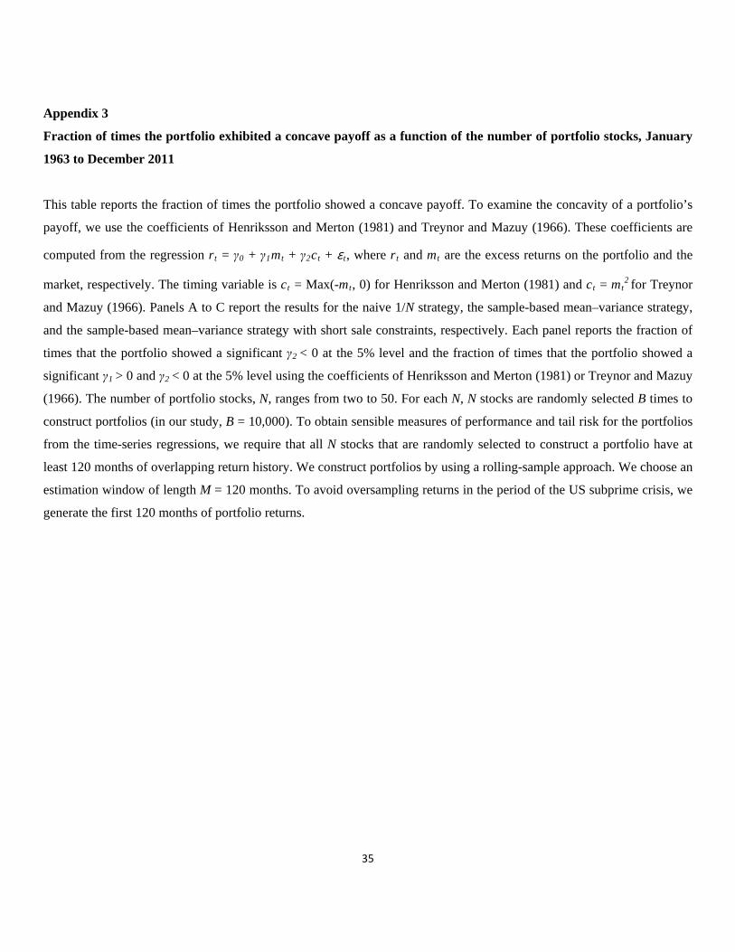
Appendix 3
Fraction of times the portfolio exhibited a concave payoff as a function of the number of portfolio stocks, January
1963 to December 2011
This table reports the fraction of times the portfolio showed a concave payoff. To examine the concavity of a portfolio’s
payoff, we use the coefficients of Henriksson and Merton (1981) and Treynor and Mazuy (1966). These coefficients are
computed from the regression rt = γ0 + γ1mt + γ2ct + ε t, where rt and mt are the excess returns on the portfolio and the
market, respectively. The timing variable is ct = Max(-mt, 0) for Henriksson and Merton (1981) and ct = mt2 for Treynor
and Mazuy (1966). Panels A to C report the results for the naive 1/N strategy, the sample-based mean–variance strategy,
and the sample-based mean–variance strategy with short sale constraints, respectively. Each panel reports the fraction of
times that the portfolio showed a significant γ2 < 0 at the 5% level and the fraction of times that the portfolio showed a
significant γ1 > 0 and γ2 < 0 at the 5% level using the coefficients of Henriksson and Merton (1981) or Treynor and Mazuy
(1966). The number of portfolio stocks, N, ranges from two to 50. For each N, N stocks are randomly selected B times to
construct portfolios (in our study, B = 10,000). To obtain sensible measures of performance and tail risk for the portfolios
from the time-series regressions, we require that all N stocks that are randomly selected to construct a portfolio have at
least 120 months of overlapping return history. We construct portfolios by using a rolling-sample approach. We choose an
estimation window of length M = 120 months. To avoid oversampling returns in the period of the US subprime crisis, we
generate the first 120 months of portfolio returns.
36
Appendix 3 (continued)
Panel A: Naive 1/N strategy Henriksson and Merton (1981) Treynor and Mazuy (1966)
N Freq
(γ2
Freq (γ<0 sig.) (%) 1>0, γ2
Freq (γ<0 sig.) (%) 2
Freq (γ<0 sig.) (%) 1>0, γ2<0 sig.) (%)
2 0.1101 0.0615 0.1377 0.1318 3 0.1286 0.0901 0.1583 0.1567 4 0.1314 0.1020 0.1678 0.1665 5 0.1474 0.1194 0.1803 0.1795 6 0.1521 0.1307 0.1952 0.1947 7 0.1571 0.1371 0.2047 0.2047 8 0.1686 0.1544 0.2138 0.2138 9 0.1727 0.1579 0.2252 0.2252
10 0.1836 0.1707 0.2338 0.2338 11 0.1878 0.1781 0.2419 0.2419 12 0.1874 0.1797 0.2420 0.2420 13 0.1940 0.1888 0.2531 0.2531 14 0.2045 0.1986 0.2644 0.2644 15 0.2111 0.2063 0.2747 0.2747 16 0.2138 0.2087 0.2796 0.2796 17 0.2181 0.2148 0.2845 0.2845 18 0.2315 0.2291 0.3005 0.3005 19 0.2292 0.2272 0.2998 0.2998 20 0.2279 0.2263 0.2976 0.2976 22 0.2384 0.2373 0.3125 0.3125 24 0.2437 0.2430 0.3200 0.3200 26 0.2553 0.2547 0.3354 0.3354 28 0.2660 0.2656 0.3464 0.3464 30 0.2683 0.2681 0.3508 0.3508 32 0.2799 0.2798 0.3630 0.3630 34 0.2810 0.2810 0.3744 0.3744 36 0.2857 0.2856 0.3678 0.3678 38 0.2876 0.2876 0.3759 0.3759 40 0.2929 0.2929 0.3842 0.3842 45 0.3066 0.3066 0.3996 0.3996 50 0.3133 0.3133 0.4142 0.4142
37
Appendix 3 (continued)
Panel B: Sample-based mean–variance strategy Henriksson and Merton (1981) Treynor and Mazuy (1966)
N Freq
(γ2
Freq (γ<0 sig.) (%) 1>0, γ2
Freq (γ<0 sig.) (%) 2
Freq (γ<0 sig.) (%) 1>0, γ2<0 sig.) (%)
2 0.1163 0.0249 0.1284 0.0940 3 0.1109 0.0281 0.1242 0.0945 4 0.1095 0.0284 0.1203 0.0913 5 0.1138 0.0249 0.1218 0.0919 6 0.1133 0.0253 0.1234 0.0938 7 0.1201 0.0215 0.1221 0.0883 8 0.1219 0.0187 0.1347 0.0980 9 0.1248 0.0174 0.1309 0.0938
10 0.1223 0.0138 0.1274 0.0928 11 0.1210 0.0122 0.1278 0.0900 12 0.1253 0.0110 0.1343 0.0903 13 0.1216 0.0087 0.1257 0.0831 14 0.1258 0.0078 0.1330 0.0902 15 0.1236 0.0066 0.1281 0.0831 16 0.1278 0.0060 0.1332 0.0791 17 0.1325 0.0055 0.1352 0.0790 18 0.1228 0.0049 0.1324 0.0754 19 0.1261 0.0024 0.1321 0.0722 20 0.1243 0.0022 0.1258 0.0702 22 0.1289 0.0017 0.1272 0.0615 24 0.1311 0.0013 0.1339 0.0648 26 0.1231 0.0004 0.1256 0.0577 28 0.1241 0.0003 0.1279 0.0537 30 0.1210 0.0001 0.1293 0.0528 32 0.1194 0.0002 0.1249 0.0477 34 0.1269 0.0001 0.1275 0.0419 36 0.1271 0.0000 0.1257 0.0391 38 0.1207 0.0001 0.1197 0.0346 40 0.1198 0.0000 0.1198 0.0327 45 0.1089 0.0000 0.1105 0.0259 50 0.1019 0.0000 0.1024 0.0228
38
Appendix 3 (continued)
Panel C: Sample-based mean–variance strategy with short sale constraints Henriksson and Merton (1981) Treynor and Mazuy (1966)
N Freq
(γ2
Freq (γ<0 sig.) (%) 1>0, γ2
Freq (γ<0 sig.) (%) 2
Freq (γ<0 sig.) (%) 1>0, γ2<0 sig.) (%)
2 0.1201 0.0578 0.1437 0.1372 3 0.1236 0.0694 0.1534 0.1500 4 0.1218 0.0729 0.1496 0.1470 5 0.1216 0.0725 0.1539 0.1511 6 0.1282 0.0803 0.1615 0.1588 7 0.1237 0.0826 0.1504 0.1489 8 0.1308 0.0888 0.1636 0.1617 9 0.1353 0.0899 0.1599 0.1588
10 0.1267 0.0891 0.1553 0.1548 11 0.1264 0.0889 0.1547 0.1536 12 0.1268 0.0896 0.1600 0.1589 13 0.1275 0.0935 0.1536 0.1528 14 0.1266 0.0887 0.1564 0.1554 15 0.1253 0.0929 0.1494 0.1486 16 0.1323 0.0983 0.1591 0.1586 17 0.1266 0.0944 0.1571 0.1569 18 0.1263 0.0902 0.1585 0.1577 19 0.1203 0.0900 0.1538 0.1534 20 0.1259 0.0953 0.1549 0.1544 22 0.1193 0.0912 0.1517 0.1511 24 0.1168 0.0890 0.1462 0.1462 26 0.1241 0.0956 0.1518 0.1515 28 0.1303 0.1022 0.1572 0.1570 30 0.1212 0.0959 0.1515 0.1514 32 0.1249 0.0982 0.1498 0.1493 34 0.1267 0.0983 0.1546 0.1543 36 0.1193 0.0969 0.1415 0.1414 38 0.1157 0.0954 0.1446 0.1445 40 0.1164 0.0936 0.1485 0.1484 45 0.1156 0.0950 0.1444 0.1444 50 0.1115 0.0924 0.1445 0.1444
39
Table 1
Extended results of DeMiguel et al. (2009b): Performance and tail risk measures for a portfolio consisting of diversified equity portfolios, January 1963 to
December 2011
This table reports the performance and tail risk measures for a portfolio consisting of diversified equity portfolios across the asset allocation models listed in
Appendix 1. The dataset we consider for the diversified equity portfolios comprises the portfolios from the Fama–French four-factor model (the FF-4-factor
dataset of DeMiguel et al., 2009b). Specifically, the dataset consists of 20 size- and book-to-market portfolios and the MKT, SMB, HML, and UMD portfolios.
The number of diversified equity portfolios in the dataset is 24. Following Wang (2005) and DeMiguel et al. (2009b), of the 25 size- and book-to-market portfolios,
we exclude the five portfolios containing the largest firms because the MKT, SMB, and HML portfolios are almost a linear combination of the 25 Fama–French
portfolios. This dataset is collected from Ken French’s website. The performance and tail risk measures we consider are the mean, standard deviation, Sharpe ratio,
CEQ return, turnover, skewness, kurtosis, historical VaR (confidence level = 95%), and historical ES (confidence level = 95%). We use all 24 assets in the dataset
to construct the portfolios. We construct the portfolios by using a rolling-sample approach, except for the sample-based mean–variance in the sample (mv - in
sample). We choose an estimation window of length M = 120 months.
Strategy Mean Standard deviation
Sharpe ratio CEQ Turnover Skewness Kurtosis VaR ES
1/N 0.0068 0.0488 0.1393 0.0056 0.0197 -0.6051 5.9441 0.0695 0.1124 mv (in sample) 0.1008 0.2012 0.5008 0.0805 - 0.1129 4.8421 0.1767 0.3408 mv 0.0780 1.0123 0.0770 -0.4344 145.4396 19.9633 420.0406 0.0742 0.4063 bs 0.0525 0.6604 0.0795 -0.1656 46.7942 19.8739 417.4976 0.0481 0.2709 dm 0.0518 0.4219 0.1227 -0.0372 59.8727 6.1453 102.3050 0.0961 0.5210 min 0.0001 0.0043 0.0124 0.0000 0.1336 0.1450 8.9281 0.0063 0.0103 mp 0.0056 0.0574 0.0972 0.0039 0.0358 -0.8088 5.5972 0.0842 0.1380 mv-c 0.0065 0.0458 0.1421 0.0055 0.2748 -0.7920 7.0535 0.0727 0.1100 bs-c 0.0066 0.0422 0.1571 0.0057 0.2315 -0.9402 8.1606 0.0679 0.1033 min-c 0.0045 0.0157 0.2887 0.0044 0.0324 -0.6739 6.6649 0.0211 0.0371 g-min-c 0.0060 0.0247 0.2417 0.0057 0.0330 -0.7985 7.2549 0.0331 0.0593 mv-min 0.0430 0.5232 0.0821 -0.0939 43.4867 19.7412 413.6792 0.0413 0.2197 ew-min 0.0001 0.0044 0.0158 0.0001 0.1331 0.1570 9.0905 0.0063 0.0103
40
Table 2
Timing coefficients for a portfolio consisting of diversified equity portfolios, January 1963 to
December 2011
This table reports the timing coefficients for a portfolio consisting of diversified equity portfolios across
the asset allocation models listed in Appendix 1. The diversified equity portfolios dataset we consider is
the set of portfolios from the Fama–French four-factor model (the FF-4 factor dataset in DeMiguel et al.,
2009b). Specifically, the dataset consists of 20 size- and book-to-market portfolios and the MKT, SMB,
HML, and UMD portfolios. The number of diversified equity portfolios in the dataset is 24. Following
Wang (2005) and DeMiguel et al. (2009b), of the 25 size- and book-to-market portfolios, we exclude the
five portfolios containing the largest firms, because the MKT, SMB, and HML portfolios are almost a
linear combination of the 25 Fama–French portfolios. This dataset is collected from Ken French’s website.
To examine the portfolio payoff concavity, we use the coefficients of Henriksson and Merton (1981) and
Treynor and Mazuy (1966). The coefficients are computed from the regression rt = γ0 + γ1mt + γ2ct + ε t,
where rt and mt are the excess returns on the portfolio and the market, respectively. The timing variable is
ct = Max(-mt, 0) for Henriksson and Merton (1981) and ct = mt2
Strategy
for Treynor and Mazuy (1966). We use
all 24 assets in the dataset to construct portfolios. We construct portfolios by using a rolling-sample
approach, except for the sample-based mean–variance in sample (mv - in sample). We choose an
estimation window of length M = 120 months. The t-statistics are given in parentheses. Numbers in bold
denote the coefficients’ statistical significance.
Henriksson and Merton (1981) Treynor and Mazuy (1966) γ γ0 γ1 γ2 γ0 γ1
1/N 2
0.0057 0.8568 -0.1660 0.0041 0.9337 -0.6007 (4.00) (23.26) (-2.76) (3.92) (47.85) (-2.82)
mv (in sample) 0.1069 0.5138 -0.5195 0.1039 0.7386 -2.8301 (7.40) (1.38) (-0.86) (9.94) (3.75) (-1.32)
mv 0.0067 4.0512 3.3301 0.0530 2.4161 6.4085 (0.09) (2.14) (1.08) (0.99) (2.41) (0.59)
bs 0.0071 2.6170 2.1073 0.0373 1.5763 3.6992 (0.15) (2.12) (1.05) (1.07) (2.41) (0.52)
dm 0.0623 0.1132 -0.6820 0.0597 0.3989 -4.2791 (2.02) (0.14) (-0.53) (2.68) (0.95) (-0.94)
min 0.0005 0.0046 -0.0309 0.0002 0.0190 -0.1028 (1.73) (0.58) (-2.39) (0.91) (4.54) (-2.25)
mp 0.0111 0.7298 -0.5410 0.0066 0.9741 -2.3335 (4.96) (12.70) (-5.77) (4.14) (32.56) (-7.16)
mv-c 0.0118 0.3892 -0.4329 0.0083 0.5833 -1.9421 (4.63) (5.95) (-4.05) (4.58) (17.01) (-5.20)
bs-c 0.0122 0.3228 -0.4308 0.0087 0.5164 -1.9126 (5.09) (5.25) (-4.29) (5.08) (16.04) (-5.45)
41
min-c 0.0080 0.0035 -0.2194 0.0057 0.1062 -0.7234 (7.71) (0.13) (-5.02) (7.51) (7.46) (-4.66)
g-min-c 0.0080 0.2740 -0.1987 0.0058 0.3676 -0.6214 (6.50) (8.70) (-3.86) (6.47) (21.94) (-3.40)
mv-min 0.0081 2.0498 1.6089 0.0320 1.2487 2.4297 (0.21) (2.10) (1.01) (1.16) (2.41) (0.43)
ew-min 0.0006 0.0066 -0.0318 0.0002 0.0214 -0.1066 (1.80) (0.83) (-2.47) (0.97) (5.12) (-2.34)
Figure 1
Return distribution of a portfolio of diversified stock portfolios
This figure shows the kernel smoothed histogram for the return distributions of portfolios consisting of
diversified stock portfolios from the naive 1/N and optimal portfolio strategies. This figure also shows the
corresponding normal distribution generated by the pooled mean and pooled standard deviation from the
return distributions of the naive 1/N and optimal portfolio strategies. The dataset we consider the
diversified stock portfolios is the set of portfolios from the Fama–French four-factor model. Specifically,
the dataset consists of 20 size- and book-to-market portfolios and the MKT, SMB, HML, and UMD
portfolios. The number of diversified assets in the dataset is 24. Following Wang (2005) and DeMiguel et
al. (2009b), of the 25 size- and book-to-market portfolios, we exclude the five portfolios containing the
largest firms, because the MKT, SMB, and HML portfolios are almost a linear combination of the 25
Fama–French portfolios. This dataset is collected from Ken French’s website. We use all 24 assets in the
dataset to construct portfolios. We construct portfolios by using a rolling-sample approach. We choose an
estimation window of length M = 120 months.
42
-0.2 -0.15 -0.1 -0.05 0 0.05 0.1 0.15 0.20
10
20
30
40
50
60
Naive portfolioMean-variance portfolioMean-variance portfolio with shortsale constraintsNormal
43
Figure 2
Performance and tail risk measures of a portfolio consisting of randomly selected stocks as a
function of the number of portfolio stocks, January 1963 to December 2011
This figure shows the mean value of the performance and tail risk measures for portfolios consisting of
randomly selected stocks from the naive 1/N and optimal portfolio strategies. The performance and tail
risk measures we consider are the mean, standard deviation, Sharpe ratio, CEQ return, turnover, MPPM
(ρ = 3), skewness, kurtosis, historical VaR (confidence level = 95%), and historical ES (confidence level
= 95%). The number of stocks in the portfolio, N, ranges from two to 50. For each N, N stocks are
randomly selected B times to construct portfolios (in our study, B = 10,000). To obtain sensible measures
of performance and tail risk for portfolios from the time-series regressions, we require that all N stocks
that are randomly selected to construct portfolios have at least 120 months of overlapping return history.
We construct portfolios by using a rolling-sample approach. We choose an estimation window of length
M = 120 months. To avoid oversampling returns in the period of the US subprime crisis, we generate the
first 120 months of portfolio returns. The dotted line in the figure shows the confidence band of each
measure. The range of the confidence band is between -2 and 2 standard deviations.
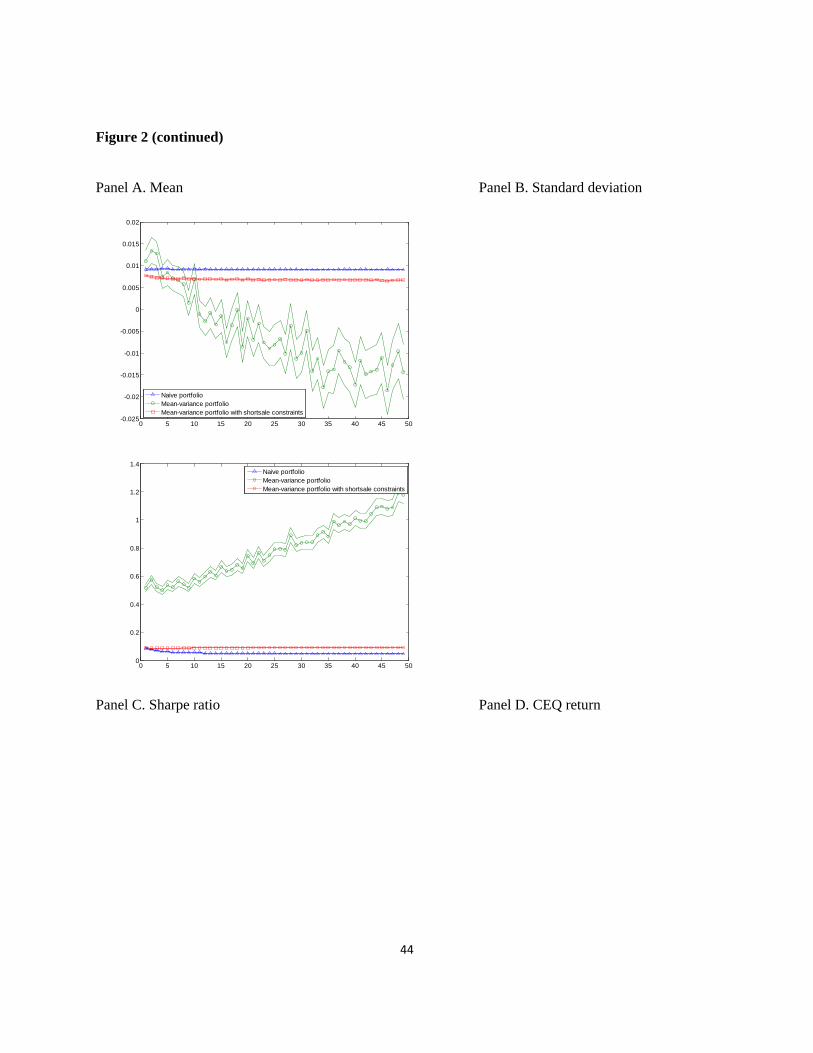
44
Figure 2 (continued)
Panel A. Mean Panel B. Standard deviation
0 5 10 15 20 25 30 35 40 45 50-0.025
-0.02
-0.015
-0.01
-0.005
0
0.005
0.01
0.015
0.02
Naive portfolioMean-variance portfolioMean-variance portfolio with shortsale constraints
0 5 10 15 20 25 30 35 40 45 500
0.2
0.4
0.6
0.8
1
1.2
1.4
Naive portfolioMean-variance portfolioMean-variance portfolio with shortsale constraints
Panel C. Sharpe ratio Panel D. CEQ return
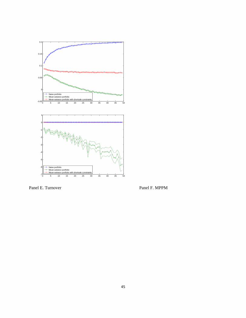
45
0 5 10 15 20 25 30 35 40 45 50-0.05
0
0.05
0.1
0.15
0.2
Naive portfolioMean-variance portfolioMean-variance portfolio with shortsale constraints
0 5 10 15 20 25 30 35 40 45 50-7
-6
-5
-4
-3
-2
-1
0
1
Naive portfolioMean-variance portfolioMean-variance portfolio with shortsale constraints
Panel E. Turnover Panel F. MPPM
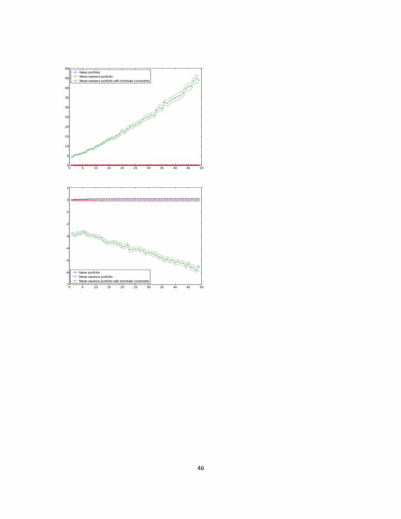
46
0 5 10 15 20 25 30 35 40 45 500
5
10
15
20
25
30
35
40
45
50
Naive portfolioMean-variance portfolioMean-variance portfolio with shortsale constraints
0 5 10 15 20 25 30 35 40 45 50-7
-6
-5
-4
-3
-2
-1
0
1
Naive portfolioMean-variance portfolioMean-variance portfolio with shortsale constraints
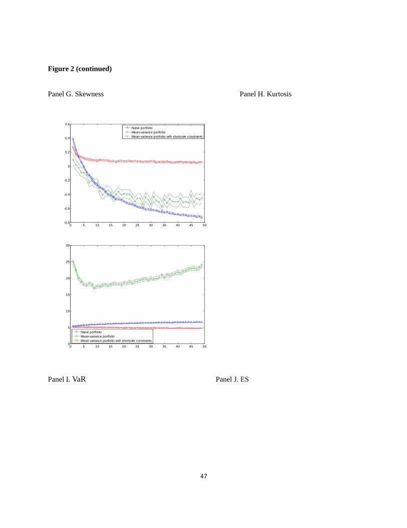
47
Figure 2 (continued)
Panel G. Skewness Panel H. Kurtosis
0 5 10 15 20 25 30 35 40 45 50-0.8
-0.6
-0.4
-0.2
0
0.2
0.4
0.6
Naive portfolioMean-variance portfolioMean-variance portfolio with shortsale constraints
0 5 10 15 20 25 30 35 40 45 500
5
10
15
20
25
30
Naive portfolioMean-variance portfolioMean-variance portfolio with shortsale constraints
Panel I. VaR Panel J. ES
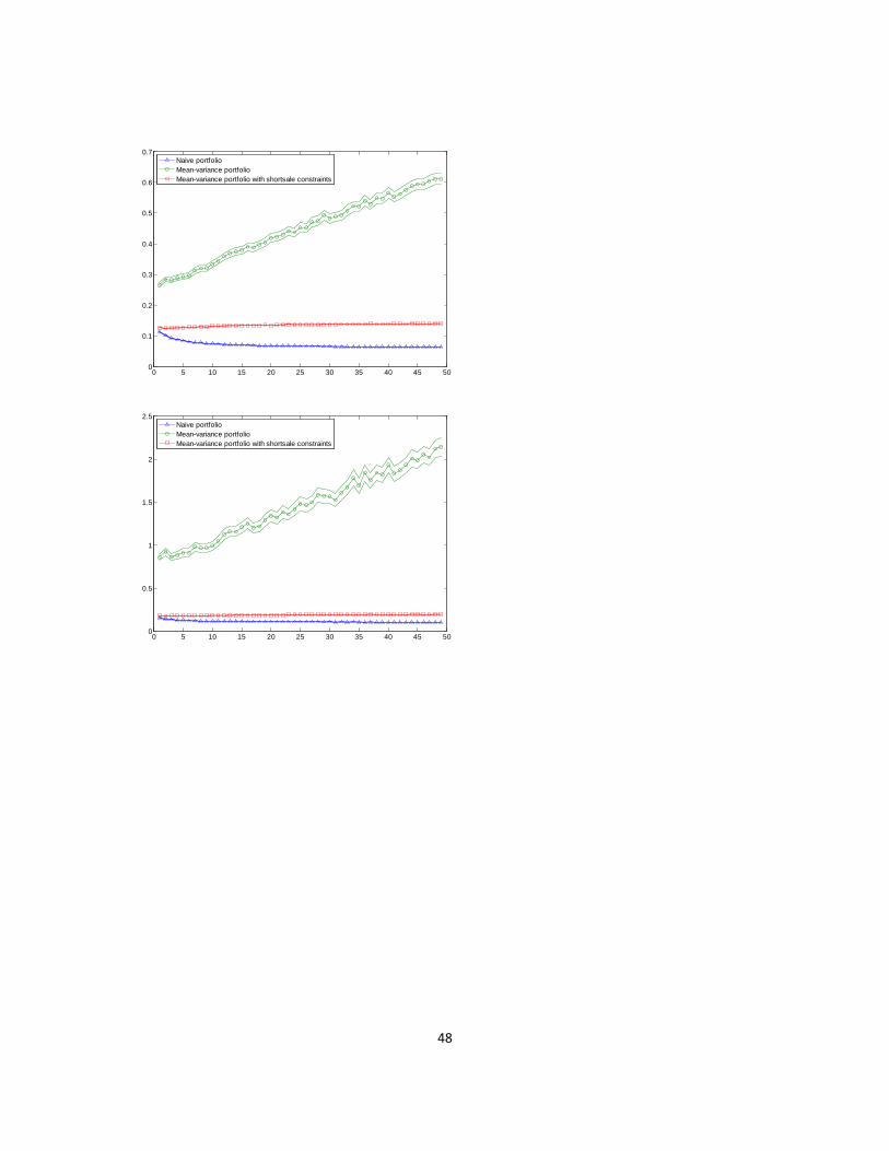
48
0 5 10 15 20 25 30 35 40 45 500
0.1
0.2
0.3
0.4
0.5
0.6
0.7
Naive portfolioMean-variance portfolioMean-variance portfolio with shortsale constraints
0 5 10 15 20 25 30 35 40 45 500
0.5
1
1.5
2
2.5
Naive portfolioMean-variance portfolioMean-variance portfolio with shortsale constraints
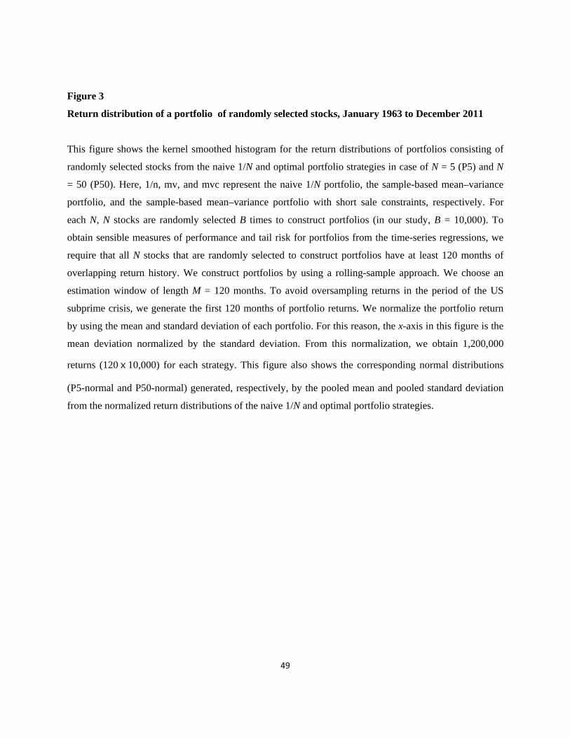
49
Figure 3
Return distribution of a portfolio of randomly selected stocks, January 1963 to December 2011
This figure shows the kernel smoothed histogram for the return distributions of portfolios consisting of
randomly selected stocks from the naive 1/N and optimal portfolio strategies in case of N = 5 (P5) and N
= 50 (P50). Here, 1/n, mv, and mvc represent the naive 1/N portfolio, the sample-based mean–variance
portfolio, and the sample-based mean–variance portfolio with short sale constraints, respectively. For
each N, N stocks are randomly selected B times to construct portfolios (in our study, B = 10,000). To
obtain sensible measures of performance and tail risk for portfolios from the time-series regressions, we
require that all N stocks that are randomly selected to construct portfolios have at least 120 months of
overlapping return history. We construct portfolios by using a rolling-sample approach. We choose an
estimation window of length M = 120 months. To avoid oversampling returns in the period of the US
subprime crisis, we generate the first 120 months of portfolio returns. We normalize the portfolio return
by using the mean and standard deviation of each portfolio. For this reason, the x-axis in this figure is the
mean deviation normalized by the standard deviation. From this normalization, we obtain 1,200,000
returns (120ⅹ10,000) for each strategy. This figure also shows the corresponding normal distributions
(P5-normal and P50-normal) generated, respectively, by the pooled mean and pooled standard deviation
from the normalized return distributions of the naive 1/N and optimal portfolio strategies.
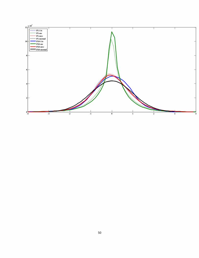
50
-4 -3 -2 -1 0 1 2 3 40
2
4
6
8
10
12x 10
4
P5-1/nP5-mvP5-mvcP5-normalP50-1/nP50-mvP50-mvcP50-normal

51
Figure 4
Fraction of times that the portfolio exhibits a concave payoff as a function of the number of
portfolio stocks, January 1963 to December 2011
This figure presents the fraction of times that the portfolio shows a concave payoff. To examine the
portfolio payoff concavity, we use the coefficients of Henriksson and Merton (1981) and Treynor and
Mazuy (1966). The coefficients are computed from the regression rt = γ0 + γ1mt + γ2ct + εt, where rt and
mt are the excess returns on the portfolio and the market, respectively. The timing variable is ct = Max(-
mt, 0) for Henriksson and Merton (1981) and ct = mt2 for Treynor and Mazuy (1966). Panels A and B
report the results for Henriksson and Merton (1981) and Treynor and Mazuy (1966), respectively. In each
panel, the upper figure shows the fraction of times that the portfolio shows a significant γ2 < 0 at the 5%
level. The lower figure shows the fraction of times that the portfolio shows a significant γ1 > 0 and γ2 < 0
at the 5% level. The number of stocks in the portfolio, N, ranges from two to 50. For each N, N stocks are
randomly selected B times to construct portfolios (in our study, B = 10,000). To obtain sensible measures
of performance and tail risk for the portfolios from the time-series regressions, we require that all N
stocks that are randomly selected to construct portfolio have at least 120 months of overlapping return
history. We construct portfolios by using a rolling-sample approach. We choose an estimation window of
length M = 120 months. To avoid oversampling returns in the period of the US subprime crisis, we
generate the first 120 months of portfolio returns.
52
Figure 4 (continued)
Panel A. Henriksson and Merton’s (1981) timing coefficients
1) Fraction of times the portfolio shows a significant γ2
0 5 10 15 20 25 30 35 40 45 500
0.05
0.1
0.15
0.2
0.25
0.3
0.35
Naive portfolioMean-variance portfolioMean-variance portfolio with shortsale constraints
< 0 at the 5% level (%)
2) Fraction of times the portfolio shows a significant γ1 > 0 and γ2 < 0 at the 5% level (%)
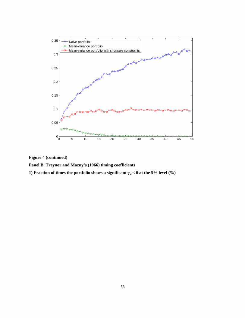
53
0 5 10 15 20 25 30 35 40 45 500
0.05
0.1
0.15
0.2
0.25
0.3
0.35
Naive portfolioMean-variance portfolioMean-variance portfolio with shortsale constraints
Figure 4 (continued)
Panel B. Treynor and Mazuy’s (1966) timing coefficients
1) Fraction of times the portfolio shows a significant γ2 < 0 at the 5% level (%)
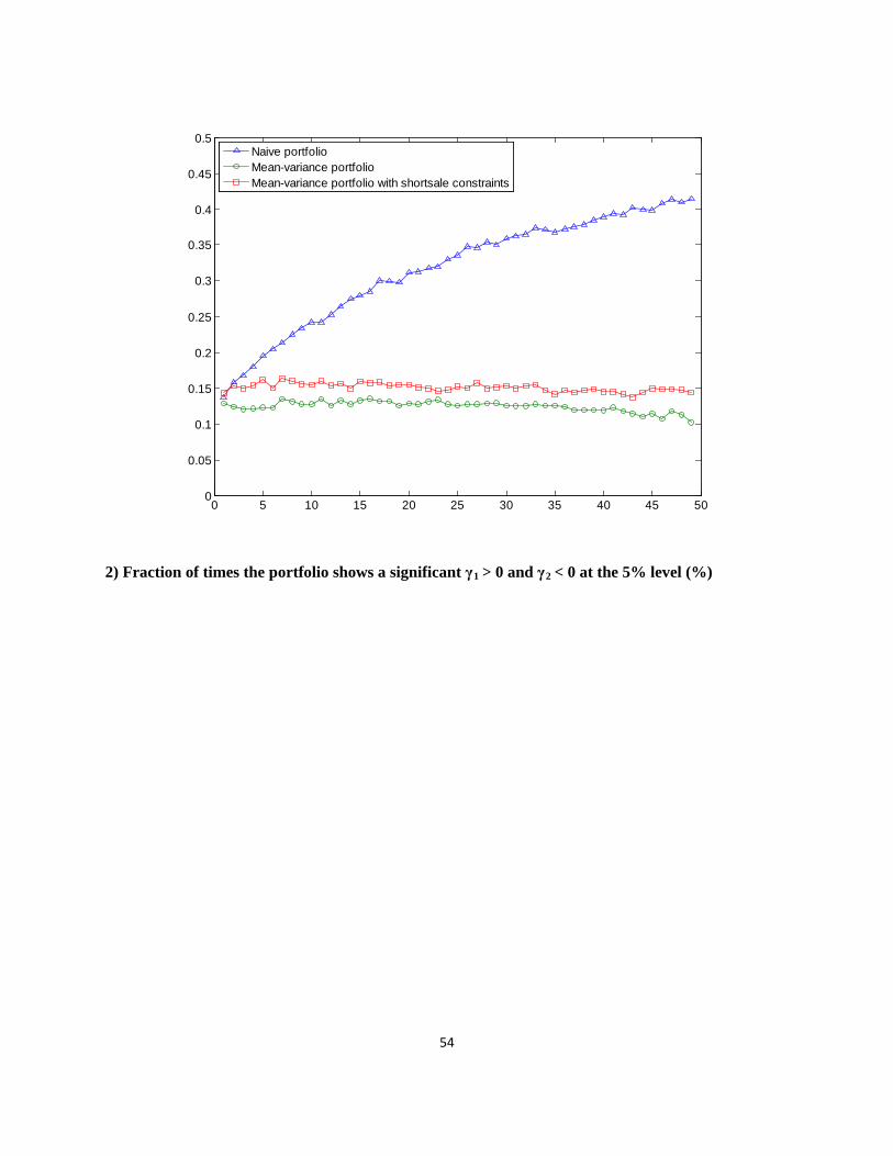
54
0 5 10 15 20 25 30 35 40 45 500
0.05
0.1
0.15
0.2
0.25
0.3
0.35
0.4
0.45
0.5
Naive portfolioMean-variance portfolioMean-variance portfolio with shortsale constraints
2) Fraction of times the portfolio shows a significant γ1 > 0 and γ2 < 0 at the 5% level (%)
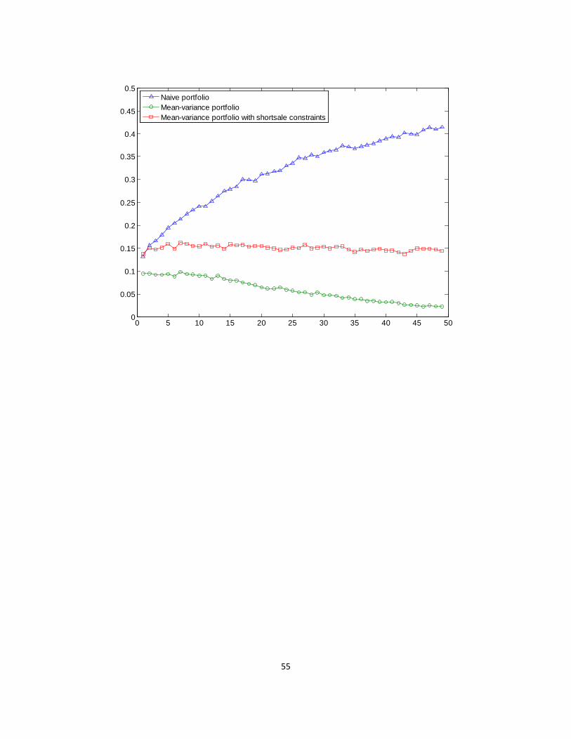
55
0 5 10 15 20 25 30 35 40 45 500
0.05
0.1
0.15
0.2
0.25
0.3
0.35
0.4
0.45
0.5
Naive portfolioMean-variance portfolioMean-variance portfolio with shortsale constraints