Why Is Africa Urbanized But Poor? Evidencefrom Resource Booms in Ghana and Ivory Coast

Remi Jedwab∗

PSE and LSE

JOB MARKET PAPER

Abstract

Africa is highly urbanized for its level of economic development. I argue thatthis paradox results from African countries exporting natural resources: re-source windfalls drive urbanization, but not necessarily long-term economicgrowth. I develop a structural transformation model where the Engel curveimplies that windfalls are disproportionately spent on urban goods and ser-vices. This drives urbanization through a rise of consumer cities. I illustratethe model by studying cocoa booms and urbanization at the district level inGhana and Ivory Coast over one century. As an identification strategy, I usethe fact that cocoa is produced by consuming the forest: (a) for agronomicreasons, farmers have to deforest a new region every 25 years, and (b) forhistorical reasons, the cocoa frontier has shifted westward in each country.I find that cities boom in newly producing regions, but persist in old onesdespite the fact those regions are poor. I discuss possible explanations forboth urban irreversibility and the lack of long-term economic growth.

JEL classification codes: O18, R00, O13, R12, N97Keywords: Urbanization, Structural Transformation, Resource Curse, Africa

∗Paris School of Economics (e-mail: jedwab@pse.ens.fr) and STICERD, London School ofEconomics (e-mail: r.c.jedwab@lse.ac.uk). I am extremely grateful to Denis Cogneau, RobinBurgess and Guy Michaels for their encouragement and support. I would like to thank DougGollin, Will Masters, Tim Besley, Sylvie Lambert, Thomas Piketty, Francois Bourguignon, Ste-fan Dercon, Marcel Fafchamps, Francis Teal, Jean-Philippe Platteau, Karen Macours, HenryOverman, Tony Venables, Gareth Austin, James Fenske, and seminar audiences at PSE, LSE,Namur, Oxford (CSAE Seminar, CSAE Conference, Oxcarre Conference), Paris (EUDN Scien-tific Conference, ABCDE World Bank), Mombasa (IGC Agriculture Workshop), Sussex, Berkeley(PACDEV) and Tinbergen (EUDN) for very helpful comments. I thank the Ivorian NationalInstitute for Statistics and the Ghanaian Statistical Service for giving me access to the surveys.I am also grateful to Francois Moriconi-Ebrard from GEOPOLIS, Vincent Anchirinah, FrancisBaah and Frederick Amon-Armah from CRIG, and Sandrine Mesple-Somps from DIAL-IRD andElise Huillery from Science-Po for their help with data collection.

“I had a marvelous dream [...]. Close to a castle, I have seen a man all dressed in

white who told me: several years ago, this region was covered with forests. It was

only missing hands to work. Compassionately, some men have come. [...] The

forest has been gradually disappearing in front of laborers, tractors have replaced

the daba [hoe] and beautiful cities, beautiful villages, beautiful roads have replaced

the tracks only practicable during the dry season.”

Houphouet-Boigny’s Presidential Address, 25 March 1974.

1 Introduction

In 1950, Sub-Saharan Africa and Asia were poor and relatively unurbanized: their

per capita GDP was less than 1,000 $1990 and their urbanization rate was around

10-15%. Interestingly, development experts were more optimistic about economic

prospects in Africa than in Asia.1 Sixty years later, Asia is three times wealthier

than Sub-Saharan Africa, but the urbanization rate is around 40% for both (see

Figure 1). Africa has thus urbanized without any concomitant increase in income.

This is at odds with historical and cross-country evidence on urbanization and

economic development (Acemoglu, Johnson and Robinson, 2002; Henderson, 2010).

What accounts for this paradox? The structural transformation literature sees

urbanization as a consequence of economic development. As a country develops,

people move out of the rural-based agricultural sector into the urban-based man-

ufacturing and service sectors. Standard models distinguish labor push and labor

pull factors as the main drivers of this transition (Alvarez-Cuadrado and Poschke,

2011). The labor push approach shows how a rise in agricultural productivity -

a green revolution - reduces the “food problem” and releases labor for the mod-

ern sector (Schultz, 1953; Gollin, Parente and Rogerson, 2002, 2007). The labor

pull approach describes how a rise in non-agricultural productivity - an industrial

revolution - attracts underemployed labor from agriculture into the modern sector

(Lewis, 1954; Harris and Todaro, 1970; Hansen and Prescott, 2002).2 Similarly, a

1I alternatively use the expressions “Sub-Saharan Africa” and “Africa” in the rest of the paper(41 countries).“Asia” includes Eastern Asia, South-Eastern Asia and South Asia (22 countries).

2A rise in manufacturing productivity also helps the modernization of agriculture throughbetter agricultural intermediate inputs. This industry-led agricultural transformation acceleratesthe structural transformation (Restuccia, Yang and Zhu, 2008; Yang and Zhu, 2010).

2

country with a comparative advantage in manufacturing or services can open up to

trade and use imports to solve its food problem (Matsuyama, 1992; Yi and Zhang,

2011). If these two approaches describe well the historical experience of developed

countries (Bairoch, 1988; Voigtlander and Voth, 2006; Allen, 2009) and successful

developing economies in Asia (Young, 2003; Bosworth and Collins, 2008; Brandt,

Hsieh and Zhu, 2008), they do not account for Africa’s urbanization.

Agricultural yields have remained low in Sub-Saharan Africa (Evenson and

Gollin, 2003; Caselli, 2005; Restuccia, Yang and Zhu, 2008). In 2009, cereal yields

were 2.8 and 5.0 times lower than in Asia and the U.S., while yields were 2.1

and 5.1 times lower for starchy roots. The African manufacturing and service

sectors are relatively small and unproductive (McMillan and Rodrik, 2011). In

2007, employment shares in industry and services were 9.6% and 25.7% for Africa,

23.9% and 34.9% for Asia and 20.6% and 78.0% in the U.S.. Labor productivity in

industry was respectively 1.7 and 15.1 times lower than in Asia and the U.S., while

labor productivity in services was respectively 3.5 and 26.0 times lower. What

has driven African urbanization? Figure 2 plots the urbanization rate and GDP

shares of “manufacturing and services” and “primary exports” (fuels, minerals

and cash crops) for Asia and Africa in 2000. While manufacturing and services

drive Asian urbanization, African urbanization is correlated with primary exports.3

If natural resource booms spur urbanization, but produce short-lived economic

growth or even economic decline due to the “resource curse” (Sachs and Warner,

2001; Robinson, Torvik and Verdier, 2006), this can solve the puzzle.4

I explore this hypothesis by developing a new structural transformation model

where resource booms lead to urbanization, through a relaxation of the “food prob-

lem”. The Engel curve implies that resource windfalls are disproportionately spent

on urban goods and services and this leads to an expansion of consumer cities. This

model is in line with the labor pull approach, except that primary exports are the

main driver of the whole process. It also shows how primary exports result in

327 out of 41 Sub-Saharan African countries and 4 out of 22 Asian countries have more than10% of their GDP originating from primary exports.

4This African paradox has been attributed to urban bias (Bates, 1981; Bairoch, 1988; Fay andOpal, 2000) or rural poverty (Barrios, Bertinelli and Strobl, 2006; Poelhekke, 2010; de Janvryand Sadoulet, 2010). Without discarding those analyzes, I wish to provide evidence for anotherchannel, natural resources. At the continental level, resource rich countries are wealthier andmore urbanized. They are also more likely to experience urbanization without growth.

3

a different type of structural change than manufacturing exports, as it produces

the following sectoral composition of cities: relatively more (non-tradable) services

and relatively less (tradable) manufacturing. I discuss how factors such as capi-

tal accumulation (e.g., durable housing and infrastructure) and the demographic

transition can result in urban irreversibility. I then discuss how limited production

linkages and rent-seeking can explain the retardation of economic growth.

I provide reduced form evidence consistent with the model by studying the

impact of cocoa production booms on urbanization in 20th century Ghana and

Ivory Coast. Figure 1 confirms that they have also experienced dramatic urban-

ization while remaining poor. I combine decadal district-level panel data on cocoa

production and cities from 1891 to 2000 for Ghana, and 1948 to 1998 in Ivory

Coast. As an identification strategy, I use the fact that cocoa is produced by

consuming the forest: (i) only forested areas are suitable to cocoa cultivation, i.e.

the South in each country, (ii) for agronomic reasons, each cocoa farmer moves to

a new forest every 25 years, thus causing regional cycles, and (iii) for historical

reasons, the cocoa front has started in the East of each country. This resulted in

the cocoa front moving across the South of each country from East to West. I can

thus instrument district production with a westward wave that I model using the

25-year agronomic cycles at the cocoa plantation level. Results suggest that local

cocoa production explains at least three-fourths of local urbanization (excluding

capital cities). Cities boom in newly producing regions, but persist in old ones

despite the fact they become poor. I provide some evidence for factors of urban

irreversibility and constraints on long-term economic growth.

In addition to the structural transformation literature, this paper is related to a

large body of work on the relationship between urbanization and growth. It could

be argued that cities promote growth in developing countries (Duranton, 2008;

Venables, 2010; McKinsey, 2011).5 Those works are based on previous studies

showing there are agglomeration economies in developed countries (Rosenthal and

Strange, 2004; Henderson, 2005; Combes et al., 2011) and developing countries (see

5For instance, McKinsey (2011) writes (p.3-19): “Africa’s long-term growth also will increas-ingly reflect interrelated social and demographic trends that are creating new engines of domesticgrowth. Chief among these are urbanization and the rise of the middle-class African consumer.[...] In many African countries, urbanization is boosting productivity (which rises as workersmove from agricultural work into urban jobs), demand and investment.”

4

Overman and Venables (2005) and Henderson (2010) for references). Yet, empirical

evidence on the positive impact of urbanization on growth is scarce (Henderson,

2003). I show that economic growth from natural resources produces a specific

type of urbanization, consisting mostly of consumer cities producing non-tradable

services. In the long run, urbanization can coexist with poverty, which casts doubt

on the ability of cities that arise due to resource booms to generate growth.

My focus on cocoa means this paper also contributes to the resource curse

literature (Sachs and Warner, 2001; Caselli and Michaels, 2009; Michaels, 2011).

Relatively little is known about the effect of cash crop windfalls (Bevan, Collier and

Gunning, 1987; Angrist and Kugler, 2008). Although the cash crop sector is also

taxed by the state, a large share of profits go to producing areas. If urbanization

can be used as a proxy for development, my study informs on the local benefits of

cash crops. Whether such effects hold in the long run is an important issue. African

countries appeared to have benefited from primary exports till the early 1980s, but

the subsequent period was characterized by macroeconomic disequilibria, social

unrest and general impoverishment. Growth has resumed, but it could be due

to favorable terms of trade. Michaels (2011) explains that resource rich regions

can have higher population densities and better infrastructure, which gives rise to

agglomeration economies. I show that producing areas are more urbanized and

have better infrastructure, but I do not find any long-term effect on per capita

income. Dercon and Zeitlin (2009) and Collier and Dercon (2009) also argue that

linkages observed in African agriculture are small.

Finally, my research is related to the literature on the respective roles of geog-

raphy and history in the spatial distribution of economic activity. The locational

fundamentals theory argues that natural advantages have a long-term impact on

economic activity (e.g. Sokoloff and Engerman, 2000; Davis and Weinstein, 2002;

Holmes and Lee, 2009; Bleakley and Lin, 2010; Nunn and Qian, 2011). The in-

creasing returns theory explains that there is path dependence in the location of

economic activity (e.g. Krugman, 1991; Rosenthal and Strange, 2004; Henderson,

2005; Combes et al., 2011; Redding, Sturm and Wolf, 2011). In my context, the

Southern forests of each country were relatively uninhabited until they provided a

natural advantage for cocoa cultivation. Booming production then launched a self-

reinforcing urbanization process. Yet, former producing regions are not wealthier

5

today, casting doubt on the existence of cumulative agglomeration effects.

The paper is organized as follows. The next section presents the background

of cocoa and cities in Ghana and Ivory Coast and the data used. In section 3,

I outline a model of structural transformation. Section 4 presents the empirical

strategy and results. Section 5 discusses the results. Section 6 concludes.

2 Background and Data

I discuss some essential features of the Ghanaian and Ivorian economies, and the

data I have collected to analyze how cash crops have contributed to urbanization.

Data Appendix A contains more details on how I construct the data.

2.1 New Data on Ghana and Ivory Coast, 1891-2000

To evaluate the impact of cash crop production on urbanization, I construct a new

panel data set on 79 Ghanaian districts, which I track almost decadally from 1891

to 2000, and 50 Ivorian districts, which I track decadally from 1948 to 1998.6 As

described below, I have collected data on cocoa production and urbanization.

I first collect data on cocoa production in tons for Ghanaian and Ivorian dis-

tricts, for as many years as possible. I use linear interpolation for missing years.

Knowing the producer price for each year, I calculate the district production value

in constant $2000. Since Ivory Coast is also a major coffee exporter, I proceed

similarly for this crop. In the end, I obtain an annual panel data set with the value

of cash crop production (cocoa and coffee) in $2000 from 1891 to 2000 in Ghana

and from 1948 to 1998 in Ivory Coast.

I then construct a GIS database of cities using census reports and administra-

tive counts. My analysis is thus limited to those years for which I have urban data:

1901, 1911, 1921, 1931, 1948, 1960, 1970, 1984 and 2000 in Ghana, and 1901, 1911,

1921, 1931, 1948, 1955, 1965, 1975, 1988 and 1998 in Ivory Coast. Historical stud-

ies on urbanization define as a city any locality with more than 5,000 inhabitants

6Ghanaian data is available using cocoa district boundaries in 1960, while Ivorian data usesadministrative district boundaries in 1998. The number of Ghanaian districts has been decreasingover time, while the number of Ivorian districts has been increasing over time. I use varioussources and GIS to reconstruct the data set using the same boundaries for the whole period.

6

(e.g. Bairoch, 1988; Acemoglu, Johnson and Robinson, 2002).7 Using the same

approach, Ghana and Ivory Coast had respectively 9 and 0 cities in 1901 and 324

cities in 2000 and 376 cities in 1998. Since I only have cash crop production data

for 79 cocoa districts in Ghana and 50 administrative districts in Ivory Coast, I

use GIS to construct district urban population for the above-mentioned years.8

I also add district total and rural populations to the Ivorian panel. This is not

possible for Ghana, as cocoa districts differ from administrative districts. Addi-

tionally, I complement the panel data set with various statistics at the country,

regional or district levels, such as income, migration and sectoral composition.

This data was obtained from household surveys, census microdata or reports,

country-level databases and agronomic studies.

2.2 Agronomic Background on Cocoa

Cocoa is produced by consuming tropical forests (Ruf, 1991, 1995a,b; Petithugh-

enin, 1995). Cocoa farmers go to a patch of virgin forest and replace forest trees

with cocoa trees. Pod production starts after 5 years, peaks after 20 and continues

up to 50 years. After 25 years, pod production has already been declining for a

few years, which farmers use as the sign to start a new cycle in a new forest.

Why is that? The forest initially provides agronomic benefits (Ruf, 1995b, p.7):

“weed control, soil fertility, protection against erosion, moisture retention for soil

and plants, protection against disease and pests, protection against drying winds,

[...] stabilizing effect on precipitation.” After 25 years, cocoa trees are too old and

the farmer can either establish a new plantation in a virgin forest or replant new

trees. But the agronomic benefits of the forest are also extinguished after 25 years

of local deforestation, and replanted cocoa trees die or are much less productive

(Petithughenin, 1995, p.96-97). Establishing a new cocoa farm in a cleared primary

forest requires 86 days of manual labor, against 168 days for manual replanting

(Ruf, 1995b, p.9). Furthermore, it is twice more expensive to opt for a replanting

strategy as intermediate inputs (fertilizers, pesticides) are needed to compensate

7Urbanization rates displayed in Figure 1 use official urban definitions, which are consistentwith the 5,000 population threshold for most census years.

8Cash crop production only booms from the 1960s in Ivory Coast. I use urban data before1948 to understand urban patterns before the boom.

7

for tree mortality and low yields (Ruf, 1995a, p.240). These agronomic cycles

at the plantation level, and the availability of forested land, explain why African

cocoa farmers have always privileged an extensive production strategy.

The aggregation of plantation cycles gives regional cycles that last several

decades (Ruf, 1995a, p.190-203). Regional production at a given point in time

is equal to cocoa land area times cocoa yields. Cocoa land area depends on the

regional forest endowment and the number of farmers, while yields reflect soil

nutrients and the age distribution of trees. Booming regions experience massive

in-migration of cocoa farmers. In the words of Ruf (1995b, p.15), “It seems that

all it takes is for people to see money from the first sale of a crop in the hands of

the first migrant planters before a cocoa migration and boom is triggered”. First,

land is cheap to buy.9 Second, farmers do not need much capital to start their own

plantation (Ruf, 1995b, p.22). Indeed, they only use land, axes, machetes, hoes,

cocoa beans and labor to produce cocoa. Lastly, yields are originally high.

A few decades later, trees are old, yields have decreased and regional production

declines. But production stagnates for a while if formerly protected forests are

open to cultivation. Cocoa cultivation is less profitable than before and farmers

must accept an income loss. Ruf (1991, p.87) writes: “Planting cocoa gives social

status, reflecting the ownership of capital yielding a huge profit. It’s the golden age

[...]. Then comes the phase of ageing cocoa trees: owning an old farm, attacked by

insects, bearing a produce whose price has fallen, does not give any status anymore.

Everything happens as if a biological curse [...] was inherent to any golden age,

as if a recession should succeed any cocoa boom.” After 25 years, a few members

of producing households move to a new forest, participating into a new regional

cycle. Here is an interesting quote of a cocoa farmer in Ruf (1991, p.107): ”An

old plantation is like an old dying wife. Medicine would be too expensive to keep

her alive. It’s better to keep the money for a younger woman [a new plantation]”.

When the forest is exhausted, cocoa moves to another country or continent.

Production was dominated by Caribbean and South American countries till the

early 20th century, then moved to Africa and is now spreading in Asia (Ruf, 1995a,

9Ruf (1995a, p.252-260) documents how the land price is initially low in unexploited forests.Migrant farmers buy large amounts of land from the chiefs of forest tribes, which causes theprice to rise. This land colonization process was then encouraged by the state. Ivorian PresidentHouphouet-Boigny liked to say that “land belongs to him who cultivates it.”

8

p.63-70). Economic and political factors can accelerate or decelerate regional cycles

(Ruf, 1995a, p.300-359): a change in the international and producer prices, land

regulations, migration policy, demographic growth, etc.

2.3 The Cash Crop Revolution in Ghana and Ivory Coast

Ghana and Ivory Coast have been two leaders of the African “cash crop revolution”

(Austin, 2008). They are the largest cocoa producers, and cocoa has been the main

motor of their economic development (Teal, 2002; Cogneau and Mesple-Somps,

2002). Figure 3 shows that production boomed after the 1920s in Ghana and the

1960s in Ivory Coast. The cocoa boom was accompanied by a coffee boom in

Ivory Coast, as cocoa farmers also produce coffee there. Cocoa and coffee have

accounted for 60.2% of exports and 20.6% of GDP in Ivory Coast in 1948-2000,

while cocoa has amounted to 56.9% of exports and 12.1% of GDP in Ghana.

The South of each country is covered with dense tropical forest, while the North

is mostly savanna. In the Southern forest, some areas are more suitable to cocoa

cultivation due to richer soil nutrients. Figure 4 shows the provinces of Ghana

and Ivory Coast, districts suitable to cocoa, highlighting highly suitable and poorly

suitable, and the two capitals, Accra and Abidjan.10 Figure 5 displays the total

value of cocoa production in 1891-2000 for each Ghanaian district and in 1948-

1998 for each Ivorian district. The comparison of Figures 4 and 5 confirms that

cocoa production has been concentrated in highly suitable districts.

Cocoa was introduced to Ghana by missionaries in 1859, but production did

not develop before 1900 (Hill, 1963; Austin, 2008). Production first spread out

in the South-East of Ghana, in the vicinity of Aburi Botanical Gardens which

were opened in 1890 (Figure 4 shows the location of Aburi). British Governor

W.B. Griffith wrote in 1888 (Hill, 1963, p.174): ”It was mainly with the view

of teaching the natives to cultivate economic plants in a systematic manner for

purposes of export that I have contemplated for some time the establishment of an

agricultural and botanical farm and garden where valuable plants could be raised

and distributed in large numbers to the people.” Cocoa seedlings were imported

10A district is suitable if more than 25% of its area consists of cocoa soils, i.e. the tropicalforest. A district is highly suitable if more than 50% of district area consists of forest ochrosols,the best cocoa soils. A district is poorly suitable if it is suitable but not highly suitable.

9

from Sao Tome and distributed to local farmers. Since cocoa cultivation was very

profitable, many farmers adopted the crop and production boomed. It peaked in

the Eastern province in 1931 (see Figures 6 and 7), before plummeting due to

the Cocoa Swollen Shoot Disease and World War II which reduced international

demand. A second cycle then started in the Ashanti province (see Figures 7, 8

and 9). But low producer prices after 1958, restrictive migratory policies after

1969 and droughts in the early 1980s precipitated the end of this cycle (see Figure

10).11 High producer prices from 1983 pushed farmers to launch a third cycle in

the Western province, the last tropical forest of Ghana (see Figure 11).

It was not till the early 1910s that the French authorities promoted cocoa

in Ivory Coast (Ruf, 1995a,b). Ivorians were originally reluctant to grow cocoa,

except in Indenie (Centre-East, see Fig. 4) where farmers heard of the wealth of

Ghanaian farmers (Ruf, 1995b, p.29). However, production did not boom until

the 1960s.12 Cocoa also moved from the East to the West (see Figures 6-11). Due

to mounting government deficits, the producer price was halved in 1989 and it

remained low thereafter, but this did not stop land colonization. Production is

now concentrated in the South-West region, the last tropical forest of Ivory Coast.

To conclude, in both countries, cocoa production was confined to the South and

started in the South-East, for exogenous reasons. Due to the 25-year agronomic

cycles at the plantation level, it moved westward (as it could not do otherwise).13

As population growth was high and cocoa was profitable, many people specialized

in it and participated to land expansion. Yet, the colonization process has not

11Ghana (from 1948) and Ivory Coast (from 1960) have fixed the producer price to protectfarmers against fluctuant international prices. The Ghana Cocoa Marketing Board (COCOBOD)and the Ivorian Caisse de stabilisation et de soutien des prix des productions agricoles (CSSPPA,or ”Caistab”) were responsible for organizing the cocoa system. Yet, since the producer price wasbelow the international price, this served as a taxation mechanism of the sector (Bates, 1981).

12Three factors explain this Ivorian ”lateness”. First, cocoa did not reach the Ghanaian borderbefore the 1910s. Second, the French forced the Ivorians to grow cocoa through a system ofmandatory labour (the corvee) and Ivorians only saw it as an European crop. Third, productionincreased in the 1920s but the boom was stopped by the Great Depression and World War II.

13Data on regional cocoa yields for post-1948 census years also displays a westward movementin yields. The largest producing region has always the highest yields. For Ghana, it was Ashantiin the 1960s (22% higher than the national average), Brong-Ahafo in the 1970s (27%) andWestern in the 1990s (40%). For Ivory Coast, it was Centre in the 1960s (32%), Centre-Westin the 1970s (19%) and early 1980s (45%), and South-West in the late 1980s (107%) and 1990s(28%). Data on regional cocoa production per rural capita confirms this analysis.

10

been as linear in Ghana as in Ivory Coast, due to natural events and economic and

political factors. Both countries have extracted almost the same quantity of cocoa

in total: 24 million tons in Ghana versus 22 in Ivory Coast. But Ivory Coast did

so in a much shorter time period. As the tropical forest is about to disappear, so

will cocoa production, unless farmers switch to intensive production strategies.14

2.4 The Urban Revolution in Ghana and Ivory Coast

While both countries were unurbanized at the turn of the 20th century, their

respective urbanization rate (using the 5,000 threshold) is 43.8% and 55.2% in

2000, making them two of the most urbanized African countries. Ghana started its

urban transition earlier than Ivory Coast, but both experienced rapid urbanization

after 1948. This is all the more impressive considering that the population of

Ghana and Ivory Coast have respectively increased by 9.7 and 15.7 times between

1900 and 2000. Ghana had 324 cities in 2000, while Ivory Coast had 376 in 1998.

Then, respectively 53.4% and 54.8% of urban inhabitants in Ghana and Ivory

Coast lived in small cities in the population range 5,000-20,000.

I calculate that national cities explain respectively 45.7% and 46.1% of urban

growth in 1901-2000 Ghana and 1948-1998 Ivory Coast.15 Respectively 66.3% and

80.0% of remaining urban growth was in areas suitable to cocoa. This strong

correlation between historical cash crop production and the emergence of cities

is documented in Figures 4 and 5. This correlation is also spatio-temporal as

cities have followed the cash crop front (see Figures 6-11). As production moves

westward, new cities appear in the West. But cities in the East do not collapse. If

anything, our analysis must account for both city formation and city persistence.

14The forested surface of Ivory Coast has decreased from 15 million hectares in 1900 to 2.5millions in 2000, while it has decreased from 9 millions in 1900 to 1.6 million in 2001 in Ghana.

15I define as national cities the capital city (Accra in Ghana, Abidjan and Yamoussoukro inIvory Coast, since Houphouet-Boigny made his village of birth the new capital in 1983) and thesecond most important city (Kumasi in Ghana, Bouake in Ivory Coast). The growth of thosecities is disconnected from the local context and entirely depends on the national context.

11

3 Model of Natural Resources and Urbanization

I now develop a model where natural resource exports generate a surplus, which is

mainly spent on urban goods and services due to the Engel curve. Urbanization is

driven by consumption linkages and takes the form of consumer cities. The model is

in line with the literature that sees the structural transformation as a consequence

of income effects (Matsuyama, 1992; Caselli and Coleman II, 2001; Gollin, Parente

and Rogerson, 2002, 2007). Non-homothetic preferences and rising incomes mean

a reallocation of expenditure shares towards urban goods and services.16 A few

models consider an open economy and look at the effects of trade on structural

transformation (Matsuyama, 1992; Echevarria, 2008; Galor and Mountford, 2008;

Matsuyama, 2009; Teigner, 2011; Yi and Zhang, 2011). Yet, in such models, man-

ufacturing exports drive urbanization. Besides, these models predict that a rise

in agricultural productivity leads to deurbanization, as the country specializes in

agricultural exports and deindustrializes. My model predicts the contrary. To

highlight the role of resource booms in urbanization as clearly as possible, the

model assumes a small open economy, only one production factor labor , and

four sectors: food, natural resources, manufacturing and services. Only services

are not tradable. The country has a comparative advantage in natural resources,

which it exports in exchange for food and manufactured goods. Resource booms

and non-homothetic preferences imply an expansion of the service sector and ur-

banization. I then discuss under which conditions natural resources can drive

urbanization while income stagnates, advancing possible explanations for urban

irreversibility and the lack of long-term economic growth.

16Other articles privileging this approach are Echevarria (1997), Laitner (2000), PiyabhaKongsamut, Sergio Rebelo and Danyang Xie (2001), Voigtlander and Voth (2006), Matsuyama(2002, 2009), Galor and Mountford (2008), Diego Restuccia, Dennis Tao Yang and Xiaodong Zhu(2008), Yang and Zhu (2010), Duarte and Restuccia (2010) and Alvarez-Cuadrado and Poschke(2011). Ngai and Pissarides (2007) and Acemoglu and Guerrieri (2008) see structural changeas a consequence of price effects: assuming a low elasticity of substitution across consumptiongoods, any relative increase in the productivity of one sector leads to a relative decrease in itsemployment share. Michaels, Rauch and Redding (2008), Buera and Kaboski (2009) and Yi andZhang (2011) adopt or compare the two approaches.

12

3.1 Set-Up

3.1.1 Technologies

The economy consists of four sectors i: food (f), natural resources (c), manufac-

turing (m) and services (s). Food, primaries and manufactured goods are tradable,

but services are not. There is one representative agent endowed with one unit of

labor. The production technologies are given by:

(1) Yi = AiLi

where Yi, Ai and Li are the output, productivity and labor share of sector i.17

Productivity is exogenous. Then, assuming the production of manufactured goods

and services is located in urban areas, the urbanization rate is Lurban = Lm+Ls.18

3.1.2 Preferences

The representative agent has the following non-homothetic preferences:

(2) U(Cf , Cc, Cm, Cs) = (Cf − Cf )αf (Cc)αc(Cm)αm(Cs)

αs

where Cf , Cc, Cm and Cs denote the consumption of food, natural resources, man-

ufactured goods and services. For the sake of simplicity, natural resources cannot

be used as intermediary goods in other sectors and only serve as consumption

goods. The sum of consumption weights is equal to one (Σiαi = 1). Cf is a food

subsistence requirement. With Cf > 0, the income elasticity of the demand for

food is below one, in line with the Engel’s law. The representative agent maximizes

her utility (2) subject to the budget constraint:

(3) w = pfCf + pcCc + pmCm + psCs

where w, pf , pc, pm and ps are the wage rate, and the prices of food, natural

resources, manufactured goods and services.

17Considering decreasing returns to scale should not change the results of the model.18This assumption is supported by the fact that the primary sector represents 87.0% and 93.9%

of rural employment in Ghana (1987-88) and Ivory Coast (1985-88). Conversely, the secondaryand tertiary sectors account for 66.8% and 76.9% of urban employment in Ghana and IvoryCoast. The model could be enriched by distinguishing urban and rural versions of each sector.

13

3.2 A Closed Subsistence Economy

3.2.1 Solving for Equilibrium

I first consider that the economy is closed. The consumer maximizes utility subject

to the budget constraint. This yields the following demands:

(4) Cf = αfw

pf+ (1− αf )Cf and Cj = αj

w

pj− αj

pfpjCf for j = {c,m, s}

The consumption of i is increasing in the wage rate w and i’s utility weight αi, and

decreasing in i’s price pi. The food subsistence requirement Cf increases food con-

sumption Cf but decreases the consumption of other goods. Perfect competition

for labor implies that:

(5) w = pfAf = pcAc = pmAm = psAs

Goods and labor markets clearing conditions are:

(6) Ci = Yi = AiLi and ΣiLi = 1

Combining (4)-(6), we find the following demands and labor shares:

(7) Cf = αfAf + (1− αf )Cf and Cj = αjAj − αjAjAf

Cf for j = {c,m, s}

(8) Lf = αf + (1− αf )CfAf

and Lj = αj − αjCfAf

for j = {c,m, s}

The food labor share is always greater than αf but converges to it as food produc-

tivity increases, since it reduces the food constraint. Conversely, the labor share

of other sectors is lower than the consumption weight, but converges to it as the

food constraint is released.

3.2.2 A Subsistence Economy

The representative agent lives at the subsistence level if food productivity is low

enough. Assuming Af = Cf , market clearing in the food sector gives:

(9) Cf = Yf = AfLf = CfLf

Consumption Cf is below the subsistence requirement Cf (and U < 0) unless

Lf = 1. In other words, when food productivity is sufficiently low, the agent only

consumes food and only works in the food sector:

14

(10) Cf = Cf and Cj = 0 for j = {c,m, s}

(11) Lf = 1 and Lj = 0 for j = {c,m, s}

This is a simple illustration of the food problem (Gollin, Parente and Rogerson,

2002, 2007): the movement of labor out of the food sector into other sectors

is constrained by the need to satisfy food requirements. The urbanization rate

Lurban = Lm +Ls is nil. Thus, there cannot be urbanization without food surplus.

3.3 Natural Resource Exports in a Small Open Economy

3.3.1 Solving for Equilibrium

I now study the pattern of structural transformation considering a small open

economy. The country takes international prices p∗f , p∗c and p∗m as given. Assum-

ing that the economy has a comparative advantage in natural resources (and a

comparative disadvantage in food and manufacturing), the autarky relative price

of natural resources is lower than the international relative price:19

(12)pcpf

<p∗cp∗f

andpcpm

<p∗mp∗m

The comparative advantage in natural resources implies that the country special-

izes in the export of natural resources and imports its consumption of food and

manufactured goods. While demands (4) are not modified, the country has two

producing sectors and perfect competition for labor means that:20

(13) w = p∗cAc = psAs

Goods and labor markets clearing conditions are:

(14) Xc + Cc = Yc = AcLc and Cs = Ys = AsLs

19There are a few reasons why the country could be “closed” before. If the economy did notknow how to produce natural resources (Ac = 0) and manufactured goods (Am = 0), and giventhat food productivity was only covering the food requirement (Af = Cf ), there was no tradeopportunity. Then, one could assume that trade costs were too high.

20The basic Ricardian trade model implies full specialization. The current model is overlysimplistic as it predicts that the domestic food and manufacturing sectors disappear. The modelcould be enriched by modeling imperfect substitutability between domestic and foreign goods ofa same sector (e.g., using Armington aggregators).

15

(15) Cf = Mf and Cm = Mm

(16) ΣiLi = 1

The balanced trade assumption stipulates that imports equal exports:

(17) p∗cXc = p∗fXf + p∗mXm

Using (4) and (13), we find that the following demands:

(18) Cf = Cf+αfp∗cAc − p∗f Cf

p∗fand Cj = αj

p∗cAc − p∗f Cfp∗j

for j = {c,m, s}

Since Cf = Af and pc

pf< p∗c

p∗f, p∗cAc − p∗f Cf > 0 and Cf > Cf . The country gains

from trade as it can now exploit its comparative advantage in natural resources.

Once the food requirement is satisfied, the share of available income p∗cAc − p∗f Cfallocated to sector i increases with i’s consumption weight αi and decreases with

i’s price pi. Combining (18) and (14)-(17), we find the following labor shares:

(19) Ls = αs(1−p∗f Cf

p∗cAc) and Lc = (1− αs)(1−

p∗f Cf

p∗cAc)︸ ︷︷ ︸

Effect A

+p∗f Cf

p∗cAc︸ ︷︷ ︸Effect B

If p∗f Cf = 0 or p∗cAc = ∞, there is no ”food problem”. A rise in natural resource

exports increases the labor share of services, which converges to the consumption

weight αs. There are then two contradictory effects on the labor share of the

natural resource sector. First, the country gets richer thanks to natural resource

exports and increases its consumption of food, natural resources and manufactur-

ing. The representative agent has then a strong incentive to work in the natural

resource sector (effect A). Second, as the country gets richer, it also increases its

consumption of services, which means a necessary reallocation of workers to the

latter sector (effect B). The second effect dominates the first, and the service sector

expands with natural resource exports. The country urbanizes, but it takes the

form of consumer cities, that consist of consumer services.21

21The model is purposely simplistic. As discussed above, the ”no manufacturing” result comesfrom the assumption that home and foreign manufactured goods are perfectly substitutable. In2000, respectively 55.1% and 64.1% of manufacturing consumption was coming from imports inGhana and Ivory Coast. For food, those shares were 12.1% and 33.8%.

16

3.3.2 Discussion

The model explains how the surplus generated by natural resource exports drives

urbanization as a result of non-homothetic preferences. But it does not tell us why

the country gets more urbanized while income stagnates. I now discuss possible

explanations for urban irreversibility and the lack of long-term economic growth.

I especially focus on the case of cocoa in Ghana and Ivory Coast.

If cities arise in new producing regions and persist in old ones, aggregate ur-

banization rises over time. Natural resources pay the fixed cost of building cities.

As production shifts westward, new cities also arise following a westward pattern.

Then, a few factors can account for urban persistence. First, if people show pref-

erence for urban living due to higher consumption amenities (“city lights”), and

if people are mobile enough to maximize utility across space, they accept a lower

income to live in town (Glaeser, Kolko and Saiz, 2001). Second, the model is

blind to capital accumulation, whether private or public. Cities are places where

people accumulate human capital and obtain higher wages (Glaeser and Mare,

2001; Lucas, 2004). Cities also have durable housing and durable infrastructure:

negative shocks reduce housing prices more than they decrease population, which

explains why urban decline is not frequent (Glaeser and Gyourko, 2005). Third,

the demographic transition can boost urban growth. If human capital accumula-

tion and health infrastructure decrease more urban mortality than they decrease

urban fertility, natural increase will multiply the effect of natural resources.

There are a few reasons why aggregate income might stagnate. First, if income

rises in booming regions but stagnates or declines in old ones, aggregate income

only slightly increases. Second, income only increases if the surplus is invested to

transform the economy. If it is consumed, if there are no production linkages from

the cocoa sector or agglomeration effects from being more urbanized, a positive

productivity shock related to cocoa only has temporary effects. Thus, a country

with a comparative advantage in natural resources experiences economic growth in

the short run. But it grows less in the long run than a country with a comparative

advantage in manufacturing, where skill accumulation, linkages and agglomeration

effects are supposedly larger (Young, 1991; Matsuyama, 1992; Galor and Mount-

ford, 2008; McMillan and Rodrik, 2011). Third, there may be negative political

17

implications of resource booms such as weak institutions, which then impacts

policies and growth (Sachs and Warner, 2001). Rent-seeking could also produce

inequality and conflict, as the political elites compete for the surplus (Robinson,

Torvik and Verdier, 2006; Angrist and Kugler, 2008; Caselli and Michaels, 2009).22

4 Method and Results

I test the hypothesis that cash crop production drives urbanization, focusing on

1891-2000 Ghana and 1948-1998 Ivory Coast. I now describe my empirical strategy

and display the results.

4.1 Panel Estimation

I run panel data regressions for districts d and years t of the following form:

(20) 4Urband,t = βd + γt + δCocoad,t + θtSd + µd,t

where βd and γt are district and year fixed effects, and my dependent variable

4Urband,t is the annual number of new urban inhabitants of district d between

each pair of years. My variable of interest Cocoad,t is the annual value of cash

crop production (in million 2000$) during the same period. µd,t are individual

disturbances clustered at the district level. I have 50 districts and 6 time periods

in Ivory Coast, hence 300 observations. I have 79 districts and 10 time periods

in Ghana, hence 790 observations. Since I look at the number of new urban

inhabitants, I drop one round and obtain respectively 250 and 711 observations.

Sd is the set of baseline controls I interact with a time trend to account for po-

tentially contaminating factors. The basic regression includes a district dummy for

containing a national city and district area. National cities (Abidjan, Bouake and

Yamoussoukro in Ivory Coast, Accra and Kumasi in Ghana) grow without it be-

ing related to local production. Other controls are: (i) Political economy: dummy

for containing a regional capital, for the same reason as for national cities; (ii)

Economic geography: dummies for having an international port, being connected

22In Web Appendix C, I discuss an extension of the model where the government taxes thecocoa sector to pay civil servants in the capital city. This leads to primacy. I also discuss therole of the capital city as a “port of entry” for traders.

18

to the railway network or the paved road network, all measured at independence

(1958 in Ghana, 1960 in Ivory Coast), as this could drive both urban growth and

production; (iii) Physical geography: dummy for being a coastal district and 1900-

2000 average annual precipitations to control for pre-existing settlement patterns.

My identification strategy exploits the fact that cocoa cultivation was confined

to the (forested) South and had to move westward in both countries, for agronomic

and historical reasons. I instrument production by a measure of the distance to the

predicted cocoa frontier, using 25-year agronomic cycles at the plantation level. I

describe at length how I construct my instrument in Web Appendix D. First, using

the GIS map of suitable area, I find that Ghana and Ivory Coast respectively had

an endowment of 896,919 and 1,462,578 plantations of 10 ha in 1900.23 Second, I

use the agronomic literature to posit that each producing household owns 10 ha

and uses it in 25 years (Ruf 1995a, p.281-283). Third, knowing the national number

of producing households for each census year and the starting point of production

in each country, I can reconstruct the predicted cocoa frontier for each year (e.g.,

the Ivorian predicted cocoa frontier is at longitude -3.34◦ in 1955, -3.57◦ in 1965,

-4.25◦ in 1975, -5.36◦ in 1988 and -6.68◦ in 1998). I create Predicted Cocoa Frontier

District Dummy, a dummy equal to one if the longitude of the centroid of district

d is less than 1◦ (≈ 110 km) from the predicted frontier. This is equivalent to

including first-order and sometimes second-order contiguous neighboring districts

of the frontier. Fourth, I expect a much smaller effect of being on the predicted

frontier for non-suitable and poorly suitable districts. That is why I instrument

cash crop production with the interaction of Predicted Cocoa Frontier District

Dummy and Highly Suitable District Dummy (see Figure 12 for an example in

1960-65). As a placebo check of my instrumentation strategy, I verify there is no

significant positive effect of Predicted Cocoa Frontier District Dummy.

4.2 Econometric Concerns

The causality is unlikely to run from cities to cash crops. First, settlement is

limited in tropical forests due to high humidity and disease incidence, and there are

few cities in regions that have not boomed yet (see Fig. 6-11). Farmers overcome

23Those figures are very close to historical approximations of the forest area in 1900: 9 millionhectares in Ghana, 15 millions in Ivory Coast.

19

these constraints when they get a high income, which is the case with cash crops.

Second, cocoa cultivation does not depend on cities for the provision of capital and

inputs, as it only requires forested land, axes, machetes, hoes, cocoa beans and

labor, and farmers use small amounts of fertilizers and insecticides. Third, West

African labor markets are highly integrated, with many laborers originating from

Northern regions or other countries. The ability of farmers to find labor thus did

not depend on urban proximity.

There could be omitted factors. First, one could argue that logging enables

cash crop production and urbanization, but farmers do not need logging companies

to cut trees. Furthermore, if logging companies open forest tracks, this might influ-

ence the location of production within districts, but it is unlikely to account for the

westward wave. Then, the export of forest products has only amounted to 10.1%

and 16.1% of exports in Ghana and Ivory Coast. Logging has been dominated by

a few parastatal companies, and profits were repatriated to national cities rather

than spent locally. Even if there were such local channels, this would not alter the

message of the paper that primary exports drives urbanization, as forestry exports

also belong to this category. My coefficients then capture the effects of cocoa,

coffee and forestry. Second, transport networks could drive both production and

urbanization. Again, while roads could influence the location of production within

districts, it cannot explain the westward wave. Cocoa beans have a high value

per ton and are easily storable. That makes cocoa “a product relatively easy to

transport, which contributes to explain the remoteness of production from roads.

[...] Very often, production precedes in time the infrastructure supposed to facil-

itate the evacuation of cocoa. [...] Migrants establish their own network of forest

tracks. As production expands, farmers widens their tracks, transform them into

motor tracks, maintain them. The State later invests to transform those tracks into

motor roads.” (Ruf, 1995b, p.334-335). I also control for infrastructure.24 Third,

local demographic growth could foster rural-urban migration and provide cheap

labor for cocoa cultivation. As argued above, settlement was limited in forested

24In Jedwab and Moradi (2011), we argue that railway construction at the beginning of the20th century has allowed cocoa farmers to start colonizing the Ashanti province (see Fig. 4).Production had to shift westward for agronomic and historical reasons, but railroads explainwhy production shifted northwestward, instead of westward or southwestward. As I instrumentproduction with a westward wave, my estimates are not contaminated by this channel.

20

areas and most migrants were coming from other regions. Integrated labor markets

imply that cocoa did not exclusively depend on local labor supply.

Lastly, the westward movement has been spatially “linear”, as no spatial jumps

are observed (see Fig. 6-11). Indeed, some farmers could have initiated another

front from the Western border rather than being on the cocoa frontier. First,

farmers spatially cluster as they belong to cooperatives, which helps them to buy

and deforest land at a lower cost. Second, most cocoa landowners are from Eastern

ethnic groups, since this is where it all began. As they still own land and have

family members (including wives and children) in the East, they commute quite

often between their two regions of residence (Hill, 1963; Ruf, 1995b). This gives

them a strong incentive to remain as close as possible to their village of origin

while looking for new plots in the West. Then, even if the westward movement

had not been linear, the instrument would instrument it with a linear movement,

which is exogenous to unobservable local factors determining spatial jumps.

4.3 Results

Table 1 presents the results for 1948-1998 Ivory Coast (columns (1)-(4)) and 1891-

2000 Ghana (columns (5)-(8)). OLS and 2SLS estimates without and with controls

are not significantly different within and across each country. Focusing on 2SLS

estimates with controls (see col. (4) and (8)), and accounting for the fact that the

2SLS estimate for Ivory Coast might be upward biased, I find that 1 million $2000

gives around 69 urban inhabitants in both countries.25

I then run a few robustness checks. Results for Ivory Coast are presented in

Table 2, while results for Ghana are presented in Table 3. Columns (1) reproduce

the main results from Table 1 (see col. (4) and (8)). First, results are robust

to using production in volume (see col. (2)). Second, I modify the definition

of the Predicted Cocoa Frontier District Dummy. Instead of considering districts

less than 1◦ (≈ 110 km) in longitude from the predicted frontier, I consider the

100 km and 50 km thresholds. If results are robust to the former (see col. (3)),

25The Kleibergen-Paap rk Wald F Stat is 9.0 for Ivory Coast, and the critical value for 15%maximal IV size is 9.0. This indicates that the IV estimate could be biased by 15-20%. If weassume conservatively that it is upward biased by 20%, this gives a coefficient of 71.2 in IvoryCoast compared to 66.8 in Ghana. The average between the two is 69.

21

estimates are 30-40% lower and only significant at 15% using the latter (see col.

(4)). 50 km is a small threshold given the average district size, and only a few

districts are selected as “treated”, which limits comparisons. Third, results are

robust to correcting for spatial autocorrelation, whether clustering at the regional

level (see col. (5)) or directly accounting for it using standard spatial techniques.26

Fourth, estimates are lower and less significant when using other urban thresholds:

10,000 (see col. (6)) and 20,000 (see col. (7)). A large share of urban growth is

coming from cities in the 5,000-20,000 population range. This also means that

local production has a large (but heterogenous) effect on cities in the 20,000-+

population range. Fifth, production has a strong impact on city formation (see

col. (8)). Lastly, I find that the cash crop effect is 4 times lower when considering

rural population in Ivory Coast as an outcome (see col. (9)), which makes the

urbanization rate increase.27

I calculate the magnitude of the cash crop effect, i.e. how much of national

urban growth over the period is attributed to this sole effect.28 Excluding national

cities, I find that cash crop production explains 73.5% of urban growth in Ivory

Coast between 1948 and 1998 and 39.4% in Ghana between 1891 and 2000. I then

investigate why magnitude is lower in Ghana. First, if I run the same regression

model with production in volume, I find that 1,000 tons of cocoa-coffee respectively

gives 118.4 and 83.6 urban inhabitants in Ivory Coast and Ghana. Given one

million $2000 of cash crop production has the same urbanization return in both

countries (69 inhabitants), the difference comes from production in volume being

relatively less profitable for Ghanaian producing areas. I calculate that Ivorian and

26I test two different approaches of spatial clustering. The plug-in HAC covariance matrixapproach is to plug-in a covariance matrix estimator that is consistent under heteroskedasticityand autocorrelation of unknown form (Conley, 1999). The cluster covariance matrix approachis to cluster observations so that group-level averages are independent. Clustering observationsusing few groups (e.g., regions) can thus ensure spatial independence (Bester, Conley and Hansen,2011). My results are robust to those various forms of clustering (results not reported butavailable upon request).

27If cash crop production increases the number of inhabitants of district d by 10,000, this couldgive one city of 10,000 or 10 villages of 1,000. This increases urban population by 10,000 in thefirst case and rural population by 10,000 in the second case.

28If δ is the impact of cocoa production on urban growth and if the total changes in urbanpopulation and cash crop production over the study period are respectively φ and τ , an approx-imation of the magnitude of this effect is τ×δ

φ ∗ 100.

22

Ghanaian farmers have respectively received 1.65 $2000 and 1.16 $2000 per ton in

the last century. This difference comes from Ivory Coast taxing relatively less its

export of cocoa and coffee, thus allowing producing areas to receive more profits

for the same output 29 If Ghanaian production had been as profitable as Ivorian

production, the magnitude would have risen to 46.5%. Second, mining (gold,

bauxite, manganese and diamonds) has represented 24.6% of Ghanaian exports

since 1948. If I run the same regression model as before but include the district

value of mining, I find that one million 2000$ of mineral production gives 15.0

urban inhabitants (significant at 1%), while the cash crop effect is unchanged. As

this effect accounts for 8.0% of local urbanization, the magnitude due to primary

exports rises to 54.4%.30

4.4 Long-Difference Estimation

As a robustness check, I run the following long-difference model for districts d:

(21) 4Urband = α + δ′Cocoad + ηSd + εd

where my dependent variable 4Urband is the annual number of new urban inhab-

itants of district d between the first and last years of the country sample (e.g.,

1891 and 2000 in Ghana). My variable of interest Cocoad is the annual value of

cash crop production (cocoa and coffee, in million 2000$) during the same period.

I have 79 districts in Ghana and 50 districts in Ivory Coast. Controls are un-

changed. I also instrument the value of cash crop production with High Suitability

Dummy, a dummy equal to one if more than 50% of district area is highly suitable

to cocoa cultivation. This instrumentation exploits the spatial discontinuity in

land suitability (see Figure 4) and echoes the strategy used by Nunn and Qian

(2011) when studying the impact of potatoes on population and urbanization. As

I relate urban change over a very long period to the total cash crop production

over the same period, δ′ captures the long-term effect of the latter on the former,

while δ from the panel estimation captures the short-term effect.

29The 1948-2000 average tax rate has been 40.5% for cocoa and coffee in Ivory Coast, and49.9% for cocoa in Ghana.

30The local urbanizing effect is much lower for mining than for cash crop production. Thisis logical if a high share of mining profits goes to the government, which then spends them innon-mining districts. Mining production is also much less labor-intensive than cocoa production.

23

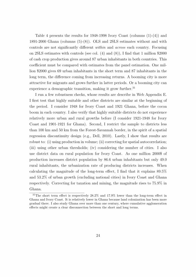
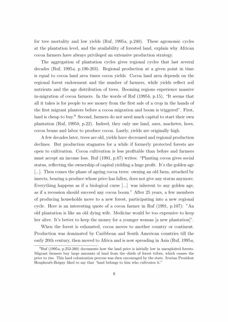
Table 4 presents the results for 1948-1998 Ivory Coast (columns (1)-(4)) and

1891-2000 Ghana (columns (5)-(8)). OLS and 2SLS estimates without and with

controls are not significantly different within and across each country. Focusing

on 2SLS estimates with controls (see col. (4) and (8)), I find that 1 million $2000

of cash crop production gives around 87 urban inhabitants in both countries. This

coefficient must be compared with estimates from the panel estimation. One mil-

lion $2000 gives 69 urban inhabitants in the short term and 87 inhabitants in the

long term, the difference coming from increasing returns. A booming city is more

attractive for migrants and grows further in latter periods. Or a booming city can

experience a demographic transition, making it grow further.31

I run a few robustness checks, whose results are describe in Web Appendix E.

I first test that highly suitable and other districts are similar at the beginning of

the period. I consider 1948 for Ivory Coast and 1921 Ghana, before the cocoa

boom in each country. I also verify that highly suitable districts do not experience

relatively more urban and rural growths before (I consider 1921-1948 for Ivory

Coast and 1901-1921 for Ghana). Second, I restrict the sample to districts less

than 100 km and 50 km from the Forest-Savannah border, in the spirit of a spatial

regression discontinuity design (e.g., Dell, 2010). Lastly, I show that results are

robust to: (i) using production in volume; (ii) correcting for spatial autocorrelation;

(iii) using other urban thresholds; (iv) considering the number of cities. I also

use district data on rural population for Ivory Coast. As one million 2000$ of

production increases district population by 86.6 urban inhabitants but only 49.0

rural inhabitants, the urbanization rate of producing districts increases. When

calculating the magnitude of the long-term effect, I find that it explains 89.5%

and 53.2% of urban growth (excluding national cities) in Ivory Coast and Ghana

respectively. Correcting for taxation and mining, the magnitude rises to 75.9% in

Ghana.

31The short term effect is respectively 28.2% and 17.9% lower than the long-term effect inGhana and Ivory Coast. It is relatively lower in Ghana because land colonization has been moregradual there. I also study Ghana over more than one century, where cumulative agglomerationeffects might create a clear disconnection between the short and long terms.

24

5 Discussion

I now discuss rural-urban linkages in newly producing regions and the long-term

effects of cash crop production, focusing on old producing regions. Due to the

poverty of data in both countries, I do not have repeated measurements of income

and other relevant dimensions at the district level and cannot carry out the same

type of estimations as for the main results. Instead, I rely on historical data at a

more aggregate spatial level and rough cross-sectional correlations on contempo-

rary data. The full analysis, including econometric results, is available in Appendix

B, while the next sections only summarize its content.

5.1 Rural-Urban Linkages in New Producing Regions

The effect of rural-based cocoa production on urban growth could be explained

either by “consumption linkages” or “production linkages”. I emphasize the former

in the model. The Engel curve implies that a disproportionate share of the cocoa

windfall is spent on urban goods and services, which gives rise to consumer cities.

If manufacturing goods are imported, the expansion of the urban sector takes the

form of non-tradable services. A related channel which is not discussed in the

model is that farmers could choose to live in town and commute to their farm

when needed. Cocoa production could then have backward production linkages,

through a higher demand for intermediate inputs, and forward production linkages,

through the development of an agro-processing sector. Urbanization then happens

through agriculture-led industrialization. I now contrast the two sets of channels.

Using as an example two regions that have recently boomed in each country,

I find that more than 1/3 of urban employment growth comes from the primary

sector (in particular cocoa farmers) and around 50% from the service sector (in

particular traders and personal service workers), while the contribution of industry

is small.32 This argues in favor of consumption linkages. I provide some evidence

that new producing regions experience a massive in-migration of cocoa farmers. As

those spend a large share of their wealth on urbanizing goods and services (“tasty

32Wholesale and retail trade and personal services account for two thirds of employment growthin the service sector. Transport, communications, education and health explain around 25%,while the contribution of business and banking services and administration is small.

25

food”, clothing, education, health, transfers and events, etc.), this is likely to drive

local urbanization. Since they spend more on services than on manufacturing

and a large share of manufactured goods are imported (around 60%), this can

potentially account for the growth of services. The fact that many cocoa farmers

live in town may also indicate a preference for urban living.

Cocoa cultivation has few backward production linkages and its production

technology has remained largely unchanged for the last century. Cultivation re-

quires only forested land, axes, machetes, hoes, cocoa beans and labor, and cocoa

farmers have made limited use of fertilizers and insecticides. Cocoa also has few

forward production linkages. Cocoa beans are not processed locally as chocolate

manufacturing is highly capital-intensive and require refrigerated factories and

ships. Profits from the cocoa sector were consumed or reinvested in land accumu-

lation, rather than used to start new sectors.

5.2 The Long-Term Effects of Cash Crop Production

Using contemporary cross-sectional data, I compare new, old and non-producing

districts along various dimensions. Interestingly, old producing districts are rela-

tively more urbanized today, despite the fact they have remained as “poor” as the

rest of the country (see Appendix B.2.1 and Appendix Tables B.1 and B.2). Their

urbanization rate is around 40-70% although their per capita income has remained

around 1,000 1990 $ (the country’s level of economic development in 1950). How

can this shed light on Figure 1, which shows that both countries have urbanized

while aggregate income has almost stagnated over half a century?

There are a few reasons why aggregate income might have stagnated. First, if

income rises in booming regions but stagnates or declines in old ones, aggregate

income only slightly increases. I document that old cocoa farms in old producing

regions have probably been reconverted to grow food crops for urban markets, thus

providing cocoa farmers with another, less profitable, source of income. Second,

aggregate income only increases if the surplus of the cocoa sector has been invested

to transform the economy. In particular, we could expect production linkages aris-

ing from the cocoa sector. But the previous analysis of rural-urban linkages, and

the fact that the sectoral composition of old producing districts is not that dif-

26

ferent from other districts (see Appendix Tables B.1 and B.2), cast doubt on the

economic significance of such linkages in this context. The employment share of

industry was still below 10% in 2000. This (lack of) new linkages is interesting,

given historical examples where natural resources had spillover effects on indus-

trialization. Wright (1981) describes how the cotton-producing South of the U.S.

developed its own textile industry from 1880, catching-up with the New England

industry. Campante and Glaeser (2009) explain that Buenos Aires and Chicago

originally grew as “conduits for moving meat and grain from fertile hinterland to

eastern markets”. It later became transformers of raw commodities and industrial

producers. Michaels (2011) shows that oil-abundant counties in the Southern U.S.

have more manufacturing today. But my result is in line with Dercon and Zeitlin

(2009) and Collier and Dercon (2009) who argue that current linkages observed in

African agriculture are small, probably due to the production structure and poor

institutions. The fact that old producing districts have urbanized without any per-

manent rise of standards of living could indicate that agglomeration economies are

limited in this context. This is contrast with Bleakley and Lin (2010) and Michaels

(2011) who show that natural advantages (portage sites or oil endowments) have

led to rising population densities and/or infrastructure investments, with positive

effects on industrialization. Third, there have been macro-institutional factors

behind the inability of the two countries to use the windfalls to transform their

economy. I describe how their institutions have remained weak. As in Sachs and

Warner (2001), their governments have sometimes adopted the “wrong” economic

policies. Then, as in Robinson, Torvik and Verdier (2006) or Caselli and Michaels

(2009), part of the windfall has been directly appropriated by the political elite.

There are then several reasons why cities persist. First, capital accumulation

make cities better places to live than villages (Glaeser, Kolko and Saiz, 2001; Lucas,

2004). I find that cities are correlated with advantages in production, such as skill

accumulation and infrastructure. But there is no direct evidence for the existence

or lack of agglomeration effects. Cities also have with advantages in consumption,

such as leisure and recreational activities, durable housing and infrastructure. I

also find that cities of the old producing regions are better places to live than other

cities. Second, I document how the demographic transition has been “urban first”

in Ghana and Ivory Coast; Natural increase the difference between fertility and

27

mortality peaked in the early 1970s for cities and the late 1980s for rural areas.

African cities are thus very different from cities of the Industrial Revolution, where

mortality was higher than in the countryside (Clark and Cummins, 2009). Using

a simple model of demographic growth, I find that natural increase has become

a significant factor in urban growth. For instance, it accounted for 45% of urban

growth in the 1990s (excluding the capital city). This means that any district

sees its urban population double in 20 years as a result of internal growth, making

urban decline very unlikely.

To conclude, in this context, resource booms have driven urbanization and

infrastructure development, but this was maybe not enough to compensate for

non-industrialization and weak institutions. Assuming two initially poor coun-

tries, the country with a comparative advantage in natural resources experiences

both economic growth and urbanization in the short term. But it grows less

in the long run than a country with a comparative advantage in manufacturing,

where skill accumulation, linkages and agglomeration effects are supposedly larger

(Young, 1991; Matsuyama, 1992; Galor and Mountford, 2008; McMillan and Ro-

drik, 2011). Despite this, it remains as urbanized. That there could be a “right”

and a “wrong” structural transformations is purely speculative and left for future

research. But it is clearly a promising avenue to understand the role of cities on

economic development.

6 Conclusion

I look at the effect of cash crop production on urbanization in two African coun-

tries, Ghana and Ivory Coast, during the 20th century. In line with the theoretical

model, I show that consumer cities arise in booming regions. Cities persist in old

producing regions although they become poor. I discuss possible explanations for

both urban irreversibility and the lack of long-term economic growth. In terms

of public policy, this means that: (i) Africa has followed a different urbanization

pattern, as its structural transformation was driven by natural resource exports;

(ii) the ability of cities to promote economic growth might depend on the type of

structural transformation. If the sectors behind the urbanization process display

small production linkages and agglomeration effects, a country can urbanize with-

28

out long-term growth; (iii) resource booms have positive economic effects in the

short term, as producing regions accumulate cities and infrastructure. But this

might not be enough to increase per capita income, probably due to missing pro-

duction linkages and weak state institutions; and (iv) natural advantages interact

with path dependence to explain the spatial distribution of economic activity.

Both countries are consuming their last tropical forest and cocoa production

will end in 20 years, unless they adopt intensive production strategies. In the mean-

time, the 2002-2011 Ivorian civil conflict was linked to the scramble for forested

land. Since independence, Baoules from the Centre region were encouraged to col-

onize the West, Northern migrants worked on Baoule farms and western Betes were

getting rich by selling land rights. This ethnic division of labor was working well

till the 1980s, when the economic crisis and land pressure fueled ethnic tensions.

Baoules and Betes complained about Northerners “stealing” their jobs, and Betes

resented the wealth of Baoules. The catalyst to the conflict was the refusal by the

government to recognize the Northern presidential candidate as “Ivorian” enough.

Ghana has not experienced any conflict, but instead has discovered offshore oil

and gas reserves. The Financial Times writes (see December 15th 2010): “Ghana

expects Jubilee’s oil and gas to help double its growth rate to more than 12 per

cent next year, funding projects to boost infrastructure and laying the foundation

for new industrial sectors.” Whether the country will experience another resource

curse is impossible to say, but the paper sheds some light on its first.

29

References

Acemoglu, Daron, and Veronica Guerrieri. 2008. “Capital Deepening andNonbalanced Economic Growth.” Journal of Political Economy, 116(3): 467–498.

Acemoglu, Daron, Simon Johnson, and James A. Robinson. 2002. “Re-versal Of Fortune: Geography And Institutions In The Making Of The ModernWorld Income Distribution.” The Quarterly Journal of Economics, 117(4): 1231–1294.

Allen, Robert. 2009. The British Industrial Revolution in Global Perspective.Cambridge: Cambridge University Press.

Alvarez-Cuadrado, Francisco, and Markus Poschke. 2011. “StructuralChange Out of Agriculture: Labor Push versus Labor Pull.” American Eco-nomic Journal: Macroeconomics, 3(3): 127–58.

Angrist, Joshua D., and Adriana D. Kugler. 2008. “Rural Windfall or a NewResource Curse? Coca, Income, and Civil Conflict in Colombia.” The Reviewof Economics and Statistics, 90(2): 191–215.

Austin, Gareth. 2008. “Resources, Techniques, and Strategies South of the Sa-hara: Revising The Factor Endowments Perspective on African Economic De-velopment, 1500-2000.” Economic History Review, 61(3): 587–624.

Bairoch, Paul. 1988. Cities and Economic Development: Frow the Dawn of His-tory to the Present. Chicago: The University of Chicago Press.

Barrios, Salvador, Luisito Bertinelli, and Eric Strobl. 2006. “ClimaticChange and Rural-Urban Migration: The Case of Sub-Saharan Africa.” Journalof Urban Economics, 60(3): 357–371.

Bateman, Merrill. 1965. Cocoa in the Ghanaian Economy. Unpublished Ph.D.dissertation, Massachussets Institute of Technology.

Bates, Robert. 1981. Markets and States in Tropical Africa: The Political Basisof Agricultural Policies. Berkeley: University of California Press.

Bester, Alan, Timothy Conley, and Christian Hansen. 2011. “Inferencewith Dependent Data Using Cluster Covariance Estimators.” Journal of Econo-metrics, Forthcoming.

Bevan, David L., Paul Collier, and Jan W. Gunning. 1987. “Consequencesof a Commodity Boom in a Controlled Economy: Accumulation and Redistri-bution in Kenya 1975-83.” World Bank Economic Review, 1(3): 489–513.

Bleakley, Hoyt, and Jeffrey Lin. 2010. “Portage: Path Dependence and In-creasing Returns in U.S. History.” NBER Working Papers 16314.

30

Bosworth, Barry, and Susan M. Collins. 2008. “Accounting for Growth:Comparing China and India.” The Journal of Economic Perspectives, 22(1): 45–66.

Brandt, Loren, Chang-Tai Hsieh, and Xiaodong Zhu. 2008. “Growth andStructural Transformation in China.” In China’s Great Economic Transforma-tion. , ed. L. Brandt and T. G. Rawski, 683–728. Cambridge: Cambridge Uni-versity Press.

Buera, Francisco J., and Joseph P. Kaboski. 2009. “Can Traditional The-ories of Structural Change Fit The Data?” Journal of the European EconomicAssociation, 7(2-3): 469–477.

Campante, Filipe, and Edward L. Glaeser. 2009. “Yet Another Tale of TwoCities: Buenos Aires and Chicago.” NBER Working Papers 15104.

Cardinal, Allan W. 1931. The Gold Coast. Government Printer.

Caselli, Francesco. 2005. “Accounting for Cross-Country Income Differences.” InHandbook of Economic Growth. Vol. 1, , ed. P. Aghion and S. Durlauf, Chapter9, 679–741. Elsevier.

Caselli, Francesco, and Guy Michaels. 2009. “Do Oil Windfalls Improve Liv-ing Standards? Evidence from Brazil.” NBER Working Papers 15550.

Caselli, Francesco, and Wilbur John Coleman II. 2001. “The U.S. Struc-tural Transformation and Regional Convergence: A Reinterpretation.” Journalof Political Economy, 109(3): 584–616.

Chaleard, Jean-Louis. 2000. Temps des villes, temps des vivres : L’Essor duvivrier marchand en Cote-d’Ivoire. Paris: Editions Karthala.

Clark, Gregory, and Neil Cummins. 2009. “Urbanization, Mortality, andFertility in Malthusian England.” American Economic Review, 99(2): 242–47.

Cogneau, Denis, and Sandrine Mesple-Somps. 2002. “L’economie ivoirienne,la fin du mirage ?” DIAL Working Papers DT/2002/18.

Collier, Paul, and Stefan Dercon. 2009. “African Agriculture in 50 Years:Smallholders in a Rapidly Changing World?” Paper prepared for the FAOExpert Meeting on How to Feed the World in 2050, FAO.

Combes, Pierre-Philippe, Gilles Duranton, Laurent Gobillon, andSebastien Roux. 2011. “Estimating Agglomeration Economies with History,Geology, and Worker Effects.” In The Economics of Agglomeration. , ed. E. L.Glaeser. NBER and University of Chicago Press.

Conley, Timothy. 1999. “GMM estimation with cross sectional dependence.”Journal of Econometrics, 92(1): 1–45.

31

Davis, Donald R., and David E. Weinstein. 2002. “Bones, Bombs, and BreakPoints: The Geography of Economic Activity.” American Economic Review,92(5): 1269–1289.

de Janvry, Alain, and Elisabeth Sadoulet. 2010. “Agriculture for Develop-ment in Africa: Business-as-Usual or New Departures?” Journal of AfricanEconomies, 19(suppl 2): ii7–ii39.

Dell, Melissa. 2010. “The Persistent Effects of Peru’s Mining Mita.” Economet-rica, 78(6): 1863–1903.

Dercon, Stefan, and Andrew Zeitlin. 2009. “Rethinking Agriculture andGrowth in Ethiopia: A Conceptual Discussion.” In Review of the AgriculturalStrategy in Ethiopia.

Dercon, Stefan, and John Hoddinott. 2005. “Livelihoods, Growth, and Linksto Market Towns in 15 Ethiopian villages.”

Dickson, Kwamina. 1968. A Historical Geography of Ghana. Cambridge: Cam-bridge University Press.

Duarte, Margarida, and Diego Restuccia. 2010. “The Role of the Struc-tural Transformation in Aggregate Productivity.” The Quarterly Journal of Eco-nomics, 125(1): 129–173.

Duranton, Gilles. 2008. “Viewpoint: From Cities to Productivity and Growthin Developing Countries.” Canadian Journal of Economics, 41(3): 689–736.

Echevarria, Cristina. 1997. “Changes in Sectoral Composition Associated withEconomic Growth.” International Economic Review, 38(2): pp. 431–452.

Echevarria, Cristina. 2008. “International trade and the sectoral compositionof production.” Review of Economic Dynamics, 11(1): 192–206.

Evenson, Robert E., and Douglas Gollin. 2003. “Assessing the Impact of theGreen Revolution, 1960 to 2000.” Science, 300(5620): 758–762.

FAO. 2010. FAOSTAT. Rome: Food and Agricultural Organization.

Fay, Marianne, and Charlotte Opal. 2000. “Urbanization without growth :a not-so-uncommon phenomenon.” The World Bank Policy Research WorkingPaper Series 2412.

Galor, Oded, and Andrew Mountford. 2008. “Trading Population for Produc-tivity: Theory and Evidence.” Review of Economic Studies, 75(4): 1143–1179.

Geopolis. 2010. Africapolis: Urbanization Trends: A Geo-Statistical Approach,West Africa. Paris: Agence Francaise de Developpement et SEDET.

32

Glaeser, Edward L., and David C. Mare. 2001. “Cities and Skills.” Journalof Labor Economics, 19(2): 316–42.

Glaeser, Edward L., and Joseph Gyourko. 2005. “Urban Decline and DurableHousing.” Journal of Political Economy, 113(2): 345–375.

Glaeser, Edward L., Jed Kolko, and Albert Saiz. 2001. “Consumer city.”Journal of Economic Geography, 1(1): 27–50.

Globcover. 2009. Globcover Africa. Louvain: European Space Agency Ionia.

Gollin, Douglas, Stephen L. Parente, and Richard Rogerson. 2002. “TheRole of Agriculture in Development.” American Economic Review, 92(2): 160–164.

Gollin, Douglas, Stephen L. Parente, and Richard Rogerson. 2007. “Thefood problem and the evolution of international income levels.” Journal of Mon-etary Economics, 54(4): 1230–1255.

Hansen, Gary D., and Edward C. Prescott. 2002. “Malthus to Solow.” Amer-ican Economic Review, 92(4): 1205–1217.

Harris, John R., and Michael P. Todaro. 1970. “Migration, Unemployment &Development: A Two-Sector Analysis.” American Economic Review, 60(1): 126–42.

Henderson, J. Vernon. 2003. “The Urbanization Process and Economic Growth:The So-What Question.” Journal of Economic Growth, 8(1): 47–71.

Henderson, J. Vernon. 2005. “Urbanization and Growth.” In Handbook of Eco-nomic Growth. Vol. 1, , ed. P. Aghion and S. Durlauf, Chapter 24, 1543–1591.Elsevier.

Henderson, J. Vernon. 2010. “Cities and Development.” Journal of RegionalScience, 50(1): 515–540.

Hill, Polly. 1963. The migrant cocoa-farmers of southern Ghana: a study in ruralcapitalism. Cambridge: Cambridge University Press.

Holmes, Thomas J., and Sanghoon Lee. 2009. “Economies of Density versusNatural Advantage: Crop Choice on the Back Forty.” NBER Working Papers14704.

Jedwab, Remi, and Alexandre Moradi. 2011. “Transportation Infrastructureand Development in Ghana.” PSE Working Papers halshs-00607207.

Kongsamut, Piyabha, Sergio Rebelo, and Danyang Xie. 2001. “BeyondBalanced Growth.” Review of Economic Studies, 68(4): 869–82.

33

Krugman, Paul. 1991. “History and Industry Location: The Case of the Manu-facturing Belt.” American Economic Review, 81(2): 80–83.

Laitner, John. 2000. “Structural Change and Economic Growth.” Review ofEconomic Studies, 67(3): 545–61.

Lewis, Arthur. 1954. “Economic Development with Unlimited Supplies ofLabour.” The Manchester School, 22(2): 139–191.

Lucas, Robert E. 2004. “Life Earnings and Rural-Urban Migration.” Journal ofPolitical Economy, 112(S1): S29–S59.

Maddison, Angus. 2008. Statistics on World Population, GDP and Per CapitaGDP, 1-2008 AD. Groningen: GGDC.

Matsuyama, Kiminori. 1992. “Agricultural Productivity, Comparative Advan-tage, and Economic Growth.” Journal of Economic Theory, 58(2): 317–334.

Matsuyama, Kiminori. 2002. “The Rise of Mass Consumption Societies.” Jour-nal of Political Economy, 110(5): 1035–1070.

Matsuyama, Kiminori. 2009. “Structural Change in an Interdependent World:A Global View of Manufacturing Decline.” Journal of the European EconomicAssociation, 7(2-3): 478–486.

McKinsey. 2011. Lions on the Move: The Progress and Potential of AfricanEconomies. London : Mc Kinsey Global Institute.

McMillan, Margaret S., and Dani Rodrik. 2011. “Globalization, StructuralChange and Productivity Growth.” NBER Working Papers 17143.

Michaels, Guy. 2011. “The Long Term Consequences of Resource-Based Special-isation.” The Economic Journal, 121(551): 31–57.

Michaels, Guy, Ferdinand Rauch, and Stephen J. Redding. 2008. “Urban-ization and Structural Transformation.” CEPR Discussion Papers 7016.

Ngai, L. Rachel, and Christopher A. Pissarides. 2007. “Structural Changein a Multisector Model of Growth.” American Economic Review, 97(1): 429–443.

Nunn, Nathan, and Nancy Qian. 2011. “The Potato’s Contribution to Popula-tion and Urbanization: Evidence from an Historical Experiment.” The QuaterlyJournal of Economics, 126(2).

Overman, Henry, and Anthony J. Venables. 2005. “Cities in the DevelopingWorld.” Centre for Economic Performance, LSE CEP Discussion Papers dp0695.

Petithughenin, Philippe. 1995. “Regeneration of Cocoa Cropping Systems: TheIvorian and Togolese Experience.” In The Economics of Cocoa Supply. , ed.Francois Ruf and P S Siswputranto. Cambridge: Woodhead Publishing Limited.

34

Petithuguenin, Philippe. 1998. “Les conditions naturelles de production ducacao en Cote d’Ivoire, au Ghana et en Indonesie.” Plantations, Recherche,Developpement, 5(6): 393–411.

Poelhekke, Steven. 2010. “Urban Growth and Uninsured Rural Risk: BoomingTowns in Bust Times.” Journal of Development Economics, In Press.

Redding, Stephen J., Daniel M. Sturm, and Nikolaus Wolf. 2011. “Historyand Industry Location: Evidence from German Airports.” Review of Economicsand Statistics, 93(3): 814–831.

Restuccia, Diego, Dennis Tao Yang, and Xiaodong Zhu. 2008. “Agricultureand aggregate productivity: A quantitative cross-country analysis.” Journal ofMonetary Economics, 55(2): 234–250.

Robinson, James A., Ragnar Torvik, and Thierry Verdier. 2006. “Po-litical foundations of the resource curse.” Journal of Development Economics,79(2): 447–468.

Rosenthal, Stuart S., and William C. Strange. 2004. “Evidence on TheNature and Sources of Agglomeration Economies.” In Handbook of Regional andUrban Economics. Vol. 4, , ed. J. V. Henderson and J. F. Thisse, Chapter 49,2119–2171. Elsevier.

Ruf, Francois. 1991. “Les crises cacaoyeres. La malediction des ages d’or ?”Cahiers d’etudes africaines, 31(121): 83–134.

Ruf, Francois. 1995a. Booms et crises du cacao: Les vertiges de l’or brun. Paris:Ministere de la Coopeeration, CIRAD-SAR and Karthala.

Ruf, Francois. 1995b. “From ”Forest Rent” to ”Tree Capital”: Basic Laws ofCocoa Supply.” In The Economics of Cocoa Supply. , ed. F. Ruf and P S Sisw-putranto. Cambridge: Woodhead Publishing Limited.

Sachs, Jeffrey D., and Andrew M. Warner. 2001. “The Curse of NaturalResources.” European Economic Review, 45(4-6): 827–838.

Schultz, Theodore W. 1953. The Economic Organization of Agriculture. NewYork: McGraw-Hill.

Sokoloff, Kenneth L., and Stanley L. Engerman. 2000. “Institutions, Fac-tor Endowments, and Paths of Development in the New World.” Journal ofEconomic Perspectives, 14(3): 217–232.

Tapinos, Georges, Philippe Hugon, and Patrice Vimard. 2003. La Coted’Ivoire a l’aube du XXIe siecle : Defis demographiques et developpementdurable. Paris: Ed. Karthala.

35

Teal, Francis J. 2002. “Export Growth and Trade Policy in Ghana in the Twen-tieth Century.” The World Economy, 25(9): 1319–1337.

Teal, Francis J., Andrew Zeitlin, and Haruna Maamah. 2006. Ghana CocoaFarmers Survey 2004: Report to Ghana Cocoa Board. CSAE-Oxford University.

Teigner, Marc. 2011. “The Role of Trade in Structural Transformation.” Un-published manuscript, University of Chicago, Department of Economics.

United Nations. 2009. World Urbanization Prospects: The 2009 Revision. NewYork: United Nations, Department of Economic and Social Affairs.

USGS. 2010. Mineral Industry Surveys 1960-2000. Reston, Virginia: U.S.G.S.

Venables, Anthony J. 2010. “Economic Geography and African Development.”Papers in Regional Science, 89(3): 469–483.

Voigtlander, Nico, and Hans-Joachim Voth. 2006. “Why England? Demo-graphic factors, structural change and physical capital accumulation during theIndustrial Revolution.” Journal of Economic Growth, 11(4): 319–361.

World Bank. 2010a. International Financial Statistics. Washington D.C.: WorldBank.

World Bank. 2010b. World Development Indicators. Washington D.C.: WorldBank.

Wright, Gavin. 1981. “Cheap Labor and Southern Textiles, 1880-1930.” TheQuarterly Journal of Economics, 96(4): 605–29.

Yang, Dennis, and Xiaodong Zhu. 2010. “Modernization of Agriculture andLong-Term Growth.” IZA Discussion Papers, 5239.

Yi, Kei-Mu, and Jing Zhang. 2011. “Structural change in an open economy.”Federal Reserve Bank of Minneapolis Staff Report, 456.

Young, Alwyn. 1991. “Learning by Doing and the Dynamic Effects of Interna-tional Trade.” The Quarterly Journal of Economics, 106(2): 369–405.

Young, Alwyn. 2003. “Gold into Base Metals: Productivity Growth in the Peo-ple’s Republic of China during the Reform Period.” Journal of Political Econ-omy, 111(6): 1220–1261.

36

Figure 1: Urbanization and Economic Development, Asia versus Africa, 1950-2010.

Sources: Maddison 2008, WUP 2009, WDI 2010, Author’s calculations. Per capita GDP datais reported in 1990 Geary-Khamis dollars (constant, PPP). The urbanization rate is reportedusing national urban definitions. This figure shows the weighted average of per capita GDP andurbanization rate for 22 Asian countries (Eastern Asia, South-Eastern Asia and South Asia) and41 Sub-Saharan Africa countries, and separately for Ghana and Ivory Coast.

Figure 2: Urbanization and Composition of GDP, Asia versus Africa, 2000.

Sources: WUP 2009, WDI 2010, USGS 2010, FAO 2010, Author’s calculations. The urban-ization rate is reported using national urban definitions. The GDP is decomposed betweenmanufacturing and services, primary exports (fuel, mining and cash crop exports) and agricul-ture (for domestic consumption). The share of agriculture in GDP is not reported. The figuredistinguishes 22 Asian countries (Eastern Asia, South-Eastern Asia and South Asia) and 41Sub-Saharan Africa countries. I display in red the quadratic prediction plots.

Figure 3: Cocoa Production, Ghana and Ivory Coast, 1900-2010.

Sources: See Data Appendix A for more details. Both countries have extracted almost the samequantity of cocoa beans throughout the 20th century: 24 million tons in Ghana, 22.1 milliontons in Ivory Coast. Production first boomed in the 1920s in Ghana, 1960s in Ivory Coast.

Figure 4: Cocoa Land Suitability and Regional and District Boundaries.

Sources: Historical soil classification maps, Globcover 2009 (see Data Appendix A for moredetails). The South of each country is covered with dense tropical forest. A district is definedas suitable if more than 25% of its area consists of cocoa soils (= tropical forest). A district isdefined as highly suitable if more than 50% of its area consists of forest ochrosols, the best cocoasoils. It is defined as poorly suitable if it is suitable, but not highly suitable.

Figure 5: Value of Cash Crop Production (1900-2000) and Cities (2000).

Note: The value of cash crop production includes the district total value (in thousand 2000$ persq.km.) of cocoa production in Ghana from 1891 to 2000, and cocoa and coffee production inIvory Coast from 1948 to 2000 (not much was produced before 1948). As there were very fewcities one century ago, cities in 2000 represent the change in urbanization over one century.

Figure 6: District Density of Cocoa Production and Cities in 1931.

Note: See Data Appendix A for more details. Production first boomed around Aburi BotanicalGardens (Eastern province) where the British colonizer has distributed cocoa seedlings to localfarmers in the 1890s. Maps for previous years (1891, 1901, 1911, 1921) are available upon request.

Figure 7: District Density of Cocoa Production and Cities in 1948.

Note: See Data Appendix A for more details.

Figure 8: District Density of Cocoa Production and Cities in 1960-1965.

Note: See Data Appendix A for more details. The map is for 1960 in Ghana and 1965 in IvoryCoast, as the population census years differ for both countries.

Figure 9: District Density of Cocoa Production and Cities in 1970-1975.

Note: See Data Appendix A for more details. The map is for 1970 in Ghana and 1975 in IvoryCoast, as the population census years differ for both countries.

Figure 10: District Density of Cocoa Production and Cities in 1984-1988.

Note: See Data Appendix A for more details. The map is for 1984 in Ghana and 1988 in IvoryCoast, as the population census years differ for both countries.

Figure 11: District Density of Cocoa Production and Cities in 1998-2000.

Note: See Data Appendix A for more details. The map is for 2000 in Ghana and 1998 in IvoryCoast, as the population census years differ for both countries.

Figure 12: Instrumentation for Cash Crop Production, 1960-1965.

Note: See Web Appendix D for more details how I construct the instrument. The map shows theinstrument (Predicted Cocoa Frontier × Highly Suitable) for 1960 in Ghana, 1965 in Ivory Coast.Knowing the total endowment of forested land, the spatial starting point of cocoa productionand the number of cocoa-producing households, and given that farmers change location every 25years for agronomic reasons, I predict the longitude of the cocoa frontier for each census year. Ithen define as Predicted Cocoa Frontier District any district which is less than 1◦ in longitudefrom the predicted cocoa frontier. As the frontier only has a large impact for highly suitabledistricts, the instrument is Predicted Cocoa Frontier × Highly Suitable. I expect no independenteffect of Predicted Cocoa Frontier District.

Tab

le1:

Cash

Cro

ps

an

dU

rban

izati

on

,P

an

el

Est

imati

on

,M

ain

Resu

lts

Dep

enden

tV

aria

ble

:D

istr

ict

Annual

Urb

anG

row

th(A

nnual

Num

ber

ofN

ewU

rban

Inhab

itan

ts,

Bet

wee

nt−

1an

dt)

Ivory

Coast

,1948-1

998

Gh

an

a,

1891-2

000

OL

SO

LS

2SL

S2S

LS

OL

SO

LS

2SL

S2S

LS

(1)

(2)

(3)

(4)

(5)

(6)

(7)

(8)

Pan

el

A:

Main

Equati

on

Dis

tric

tA

nnual

Val

ue

ofC

ash

Cro

pP

rod.

107.

5***

73.8

***

166.

9**

89.0

**24

.9**

24.0

*65

.0*

66.8

*(M

illion

sof

2000

$,B

etw

eent−

1an

dt)

(19.

8)(1

5.0)

(82.

7)(4

3.2)

(11.

6)(1

3.2)

(38.

5)(3

8.4)

Pre

dic

ted

Coco

aF

ronti

erD

istr

ict

Dum

my

-1,0

35.5

-154

.6-4

88.2

-494

.9(D

istr

ict

Lon

gitu

de≤

1◦fr

omP

redic

ted

Coco

aF

ronti

er)

(1,2

60.4

)(4

94.2

)(3

99.0

)(3

61.5

)

Pan

el

B:

Fir

stSta

ge

Pre

dic

ted

Coco

aF

ronti

erD

ist.×

Hig

hly

Suit

able

Dis

t.D

um

my

20.0

***

16.6

***

13.0

***

12.9

***

(6.6

)(5

.3)

(1.8

)(1

.8)

Pre

dic

ted

Coco

aF

ronti

erD

istr

ict

Dum

my

-2.8

-0.6

-0.9

*-1

.2**

(Dis

tric

tL

ongi

tude≤

1◦fr

omP

redic

ted

Coco

aF

ronti

er)

(3.2

)(2

.3)

(0.5

)(0

.5)

Kle

iber

gen-P

aap

rkW

ald

FSta

t8.

69.

050

.451

.5O

bse

rvat

ions

250

250

250

250

711

711

711

711

R-s

quar

ed0.

530.

810.

510.

810.

650.

670.

650.

67D

istr

ict

and

Yea

rF

ixed

Eff

ects

YY

YY

YY

YY

Bas

elin

eC

ontr

ols×

Yea

rN

YN

YN

YN

Y

Not

es:

Rob

ust

stan

dard

erro

rscl

uste

red

atth

edi

stri

ctle

vel

inpa

rent

hese

s.*

sign

ifica

ntat

10%

;**

sign

ifica

ntat

5%;

***

sign

ifica

ntat

1%.

The

rear

e50

dist

rict

san

d6

year

sin

Ivor

yC

oast

,and

79di

stri

cts

and

10ye

ars

inG

hana

.Si

nce

Ilo

okat

the

num

ber

ofne

wur

ban

inha

bita

nts,

Idr

opon

ero

und.

All

regr

essi

ons

incl

ude

dist

rict

and

year

fixed

effec

ts,

and

adu

mm

yeq

ual

toon

eif

the

dist

rict

cont

ains

ana

tion

alci

tyan

ddi

stri

ctar

ea(s

qkm

).D

istr

ict

Ann

ual

Urb

anG

row

this

the

annu

alnu

mbe

rof

new

urba

nin

habi

tant

sin

the

dist

rict

betw

eent−

1an

dt.

Dis

tric

tA

nnua

lVal

ueof

Cas

hC

rop

Pro

d.is

the

annu

alva

lue

ofca

shcr

oppr

oduc

tion

inth

edi

stri

ctbe

twee

nt−

1an

dt.

Pre

dict

edC

ocoa

Fron

tier

Dis

t.×

Hig

hly

Suit

able

Dis

t.D

umm

yis

adu

mm

yeq

ualt

oon

eif

the

dist

rict

ishi

ghly

suit

able

and

its

long

itud

e(m

easu

reby

its

cent

roid

)is

less

than

1◦fr

omth

epr

edic

ted

coco

afr

onti

er(≈

110

km).

Adi

stri

ctis

high

lysu

itab

leif

mor

eth

an50

%of

its

area

cons

ists

offo

rest

ochr

osol

s.I

incl

ude

vari

ous

cont

rols

.P

olit

ical

econ

omy:

adu

mm

yeq

ual

toon

eif

the

dist

rict

cont

ains

are

gion

alca

pita

l.E

cono

mic

geog

raph

y:du

mm

ies

for

whe

ther

the

dist

rict

has

apa

ved

road

,a

railw

ayor

anin

tern

atio

nal

port

atin

depe

nden

ce(1

958

inG

hana

,19

60in

Ivor

yC

oast

).P

hysi

cal

geog

raph

y:di

stri

ctdu

mm

yfo

rbe

ing

aco

asta

ldi

stri

ctan

d19

00-2

000

aver

age

annu

alpr

ecip

itat

ions

(mm

).D

ata

App

endi

xA

expl

ains

inde

tails

how

Ico

nstr

uct

the

vari

able

s.

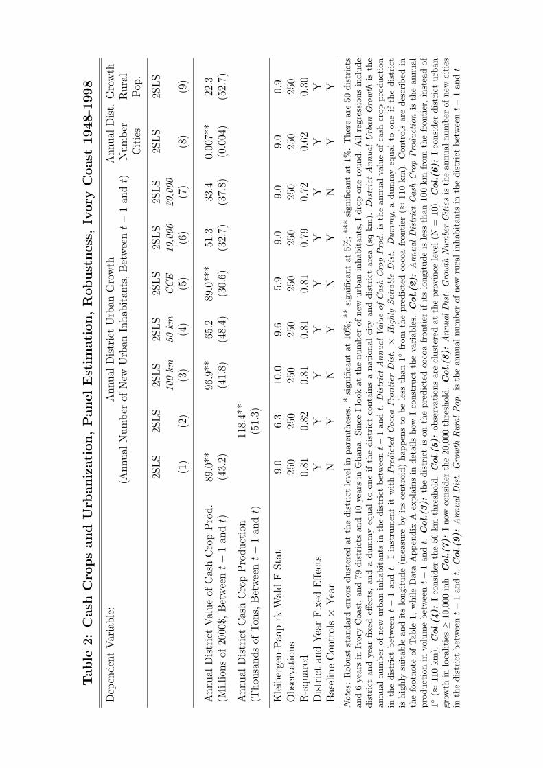
Tab

le2:

Cash

Cro

ps

an

dU

rban

izati

on

,P

an

el

Est

imati

on

,R

ob

ust

ness

,Iv

ory

Coast

1948-1

998

Dep

enden

tV

aria

ble

:A

nnual

Dis

tric

tU

rban

Gro

wth

Annual

Dis

t.G

row

th(A

nnual

Num

ber

ofN

ewU

rban

Inhab

itan

ts,

Bet

wee

nt−

1an

dt)

Num

ber

Cit

ies

Rura

lP

op.

2SL

S2S

LS

2SL

S2S

LS

2SL

S2S

LS

2SL

S2S

LS

2SL

S10

0km

50km

CC

E10

,000

20,0

00(1

)(2

)(3

)(4

)(5

)(6

)(7

)(8

)(9

)

Annual

Dis

tric

tV

alue

ofC

ash

Cro

pP

rod.

89.0

**96

.9**

65.2

89.0

***

51.3

33.4

0.00

7**

22.3

(Million

sof

2000

$,B

etw

eent−

1an

dt)

(43.

2)(4

1.8)

(48.

4)(3

0.6)

(32.

7)(3

7.8)

(0.0

04)

(52.

7)

Annual

Dis

tric

tC

ash

Cro

pP

roduct

ion

118.

4**

(Thou

sands

ofT

ons,

Bet

wee

nt−

1an

dt)

(51.

3)

Kle

iber

gen-P

aap

rkW

ald

FSta

t9.

06.

310

.09.

65.

99.

09.

09.

00.

9O

bse

rvat

ions

250

250

250

250

250

250

250

250

250

R-s

quar

ed0.

810.

820.

810.

810.

810.

790.

720.

620.

30D

istr

ict

and

Yea

rF

ixed

Eff

ects

YY

YY

YY

YY

YB

asel

ine

Con

trol

s×

Yea

rN

YN

YN

YN

YY

Not

es:

Rob

ust

stan

dard

erro

rscl

uste

red

atth

edi

stri

ctle

vel

inpa

rent

hese

s.*

sign

ifica

ntat

10%

;**

sign

ifica

ntat

5%;

***

sign

ifica

ntat

1%.

The

rear

e50

dist

rict

san

d6

year

sin

Ivor

yC

oast

,and

79di

stri

cts

and

10ye

ars

inG

hana

.Si

nce

Ilo

okat

the

num

ber

ofne

wur

ban

inha

bita

nts,

Idr

opon

ero

und.

All

regr

essi

ons

incl

ude

dist

rict

and

year

fixed

effec

ts,

and

adu

mm

yeq

ual

toon

eif

the

dist

rict

cont

ains

ana

tion

alci

tyan

ddi

stri

ctar

ea(s

qkm

).D

istr

ict

Ann

ual

Urb

anG

row

this

the

annu

alnu

mbe

rof

new

urba

nin

habi

tant

sin

the

dist

rict

betw

eent−

1an

dt.

Dis

tric

tA

nnua

lVal

ueof

Cas

hC

rop

Pro

d.is

the

annu

alva

lue

ofca

shcr

oppr

oduc

tion

inth

edi

stri

ctbe

twee

nt−

1an

dt.

Iin

stru

men

tit

wit

hP

redi

cted

Coc

oaFr

onti

erD

ist.×

Hig

hly

Suit

able

Dis

t.D

umm

y,a

dum

my

equa

lto

one

ifth

edi

stri

ctis

high

lysu

itab

lean

dit

slo

ngit

ude

(mea

sure

byit

sce

ntro

id)

happ

ens

tobe

less

than

1◦fr

omth

epr

edic

ted

coco

afr

onti

er(≈

110

km).

Con

trol

sar

ede

scri

bed

inth

efo

otno

teof

Tab

le1,

whi

leD

ata

App

endi

xA

expl

ains

inde

tails

how

Ico

nstr

uct

the

vari

able

s.Col.(2

):A

nnua

lD

istr

ict

Cas

hC

rop

Pro

duct

ion

isth

ean

nual

prod

ucti

onin

volu

me

betw

eent−

1an

dt.

Col.(3

):th

edi

stri

ctis

onth

epr

edic

ted

coco

afr

onti

erif

its

long

itud

eis

less

than

100

kmfr

omth

efr

onti

er,

inst

ead

of1◦

(≈11

0km

).Col.(4

):I

cons

ider

the

50km

thre

shol

d.Col.(5

):ob

serv

atio

nsar

ecl

uste

red

atth

epr

ovin

cele

vel

(N=

10).

Col.(6

):I

cons

ider

dist

rict

urba

ngr

owth

inlo

calit

ies≥

10,0

00in

h.Col.(7

):I

now

cons

ider

the

20,0

00th

resh

old.

Col.(8

):A

nnua

lDis

t.G

row

thN

umbe

rC

itie

sis

the

annu

alnu

mbe

rof

new

citi

esin

the

dist

rict

betw

eent−

1an

dt.

Col.(9

):A

nnua

lD

ist.

Gro

wth

Rur

alP

op.

isth

ean

nual

num

ber

ofne

wru

ral

inha

bita

nts

inth

edi

stri

ctbe

twee

nt−

1an

dt.

Tab

le3:

Cash

Cro

ps

an

dU

rban

izati

on

,P

an

el

Est

imati

on

,R

ob

ust

ness

,G

han

a1891-2

000

Dep

enden

tV

aria

ble

:A

nnual

Dis

tric

tU

rban

Gro

wth

Annual

Dis

t.G

row

th(A

nnual

Num

ber

ofN

ewU

rban

Inhab

itan

ts,

Bet

wee

nt−

1an

dt)

Num

ber

Cit

ies

Rura

lP

op.

2SL

S2S

LS

2SL

S2S

LS

2SL

S2S

LS

2SL

S2S

LS

2SL

S10

0km

50km

CC

E10

,000

20,0

00(1

)(2

)(3

)(4

)(5

)(6

)(7

)(8

)(9

)

Annual

Dis

tric

tV

alue

ofC

ash

Cro

pP

rod.

66.8

*75

.6*

40.5

66.8

**55

.244

.40.

003*

(Million

sof

2000

$,B

etw

eent−

1an

dt)

(38.

4)(4

2.1)

(27.

6)(3

0.6)

(37.

4)(3

6.2)

(0.0

01)

Annual

Dis

tric

tC

ash

Cro

pP

roduct

ion

83.6

*(T

hou

sands

ofT

ons,

Bet

wee

nt−

1an

dt)

(48.

5)

Kle

iber

gen-P

aap

rkW

ald

FSta

t51

.538

.542

.041

.011

3.1

51.5

51.5

51.5

Obse

rvat

ions

711

711

711

711

711

711

711

711

R-s

quar

ed0.

670.

670.

670.

670.

480.

670.

670.

26D

istr

ict

and

Yea

rF

ixed

Eff

ects

YY

YY

YY

YY

Bas

elin

eC

ontr

ols×

Yea

rN

YN

YN

YN

Y

Not

es:

Rob

ust

stan

dard

erro

rscl

uste

red

atth

edi

stri

ctle

vel

inpa

rent

hese

s.*

sign

ifica

ntat

10%

;**

sign

ifica

ntat

5%;

***

sign

ifica

ntat

1%.

The

rear

e50

dist

rict

san

d6

year

sin

Ivor

yC

oast

,and

79di

stri

cts

and

10ye

ars

inG

hana

.Si

nce

Ilo

okat

the

num

ber

ofne

wur

ban

inha

bita

nts,

Idr

opon

ero

und.

All

regr

essi

ons

incl

ude

dist

rict

and

year

fixed

effec

ts,

and

adu

mm

yeq

ual

toon

eif

the

dist

rict

cont

ains

ana

tion

alci

tyan

ddi

stri

ctar

ea(s

qkm

).D

istr

ict

Ann

ual

Urb

anG

row

this

the

annu

alnu

mbe

rof

new

urba

nin

habi

tant

sin

the

dist

rict

betw

eent−

1an

dt.

Dis

tric

tA

nnua

lVal

ueof

Cas

hC

rop

Pro

d.is

the

annu

alva

lue

ofca

shcr

oppr

oduc

tion

inth

edi

stri

ctbe

twee

nt−

1an

dt.

Iin

stru

men

tit

wit

hP

redi

cted

Coc

oaFr

onti

erD

ist.×

Hig

hly

Suit

able

Dis

t.D

umm

y,a

dum

my

equa

lto

one

ifth

edi

stri

ctis

high

lysu

itab

lean

dit

slo

ngit

ude

(mea

sure

byit

sce

ntro

id)

happ

ens

tobe

less

than

1◦fr

omth

epr

edic

ted

coco

afr

onti

er(≈

110

km).

Con

trol

sar

ede

scri

bed

inth

efo

otno

teof

Tab

le1,

whi

leD

ata

App

endi

xA

expl

ains

inde

tails

how

Ico

nstr

uct

the

vari

able

s.Col.(2

):A

nnua

lD

istr

ict

Cas

hC

rop

Pro

duct

ion

isth

ean

nual

prod

ucti

onin

volu

me

betw

eent−

1an

dt.

Col.(3

):th

edi

stri

ctis

onth

epr

edic

ted

coco

afr

onti

erif

its

long

itud

eis

less

than

100

kmfr

omth

efr

onti

er,

inst

ead

of1◦

(≈11

0km

).Col.(4

):I

cons

ider

the

50km

thre

shol

d.Col.(5

):ob

serv

atio

nsar

ecl

uste

red

atth

epr

ovin

cele

vel

(N=

10).

Col.(6

):I

cons

ider

dist

rict

urba

ngr

owth

inlo

calit

ies≥

10,0

00in

h.Col.(7

):I

now

cons

ider

the

20,0

00th

resh

old.

Col.(8

):A

nnua

lDis

t.G

row

thN

umbe

rC

itie

sis

the

annu

alnu

mbe

rof

new

citi

esin

the

dist

rict

betw

eent−

1an

dt.

Col.(9

):A

nnua

lD

ist.

Gro

wth

Rur

alP

op.:

this

dist

rict

vari

able

isno

tav

aila

ble

for

Gha

na.

Tab

le4:

Cash

Cro

ps

an

dU

rban

izati

on

,L

on

g-D

iffere

nce

Est

imati

on

,M

ain

Resu

lts

Dep

enden

tV

aria

ble

:D

istr

ict

Annual

Urb

anG

row

th(A

nnual

Num

ber

ofN

ewU

rban

Inhab

itan

ts,

Bet

wee

nt 0

andT

)

Ivory

Coast

,1948-1

998

Gh

an

a,

1891-2

000

OL

SO

LS

2SL

S2S

LS

OL

SO

LS

2SL

S2S

LS

(1)

(2)

(3)

(4)

(5)

(6)

(7)

(8)

Panel

A:

Main

Equati

on

Dis

tric

tA

nnual

Val

ue

ofC

ash

Cro

pP

rod.

133.

6**

100.

6***

71.0

***

86.6

***

63.9

***

82.0

***

74.5

***

87.3

***

(Million

sof

2000

$,B

etw

eent 0

andT

)(5

7.7)

(23.

0)(2

0.9)

(31.

3)(1

5.7)

(18.

4)(1

8.8)

(23.

0)

Panel

B:

Fir

stSta

ge

Hig

hly

Suit

able

Dis

tric

tD

um

my

26.1

***

24.6

***

9.1*

**7.

8***

(5.2

)(4

.5)

(1.0

)(1

.1)

Kle

iber

gen-P

aap

rkW

ald

FSta

t23

.623

.764

.143

.9O

bse

rvat

ions

5050

5050

7979

7979

R-s

quar

ed0.

560.

810.

540.

810.

860.

900.

860.

90B

asel

ine

Con

trol

sN

YN

YN

YN

Y

Not

es:

Rob

ust

stan

dard

erro

rsin

pare

nthe

ses.

*si

gnifi

cant

at10

%;*

*si

gnifi

cant

at5%

;***

sign

ifica

ntat

1%.

The

rear

e50

dist

rict

sin

Ivor

yC

oast

,and

79di

stri

cts

inG

hana

.A

llre

gres

sion

sin

clud

ea

dum

my

equa

lto

one

ifth

edi

stri

ctco

ntai

nsa

nati

onal

city

and

dist

rict

area

(sq

km).

Dis

tric

tA

nnua

lU

rban

Gro

wth

isth

ean

nual

num

ber

ofne

wur

ban

inha

bita

nts

inth

edi

stri

ctbe

twee

nt 0

andT

,the

first

and

the

last

year

sof

the

data

set:

1948

and

1998

for

Ivor

yC

oast

,189

1an

d20

00fo

rG

hana

.D

istr

ict

Ann

ual

Val

ueof

Cas

hC

rop

Pro

d.is

the

annu

alva

lue

ofca

shcr

oppr

oduc

tion

inth

edi

stri

ctbe

twee

nt 0

andT

.I

inst

rum

ent

itw

ith

Hig

hly

Suit

able

Dis

tric

tD

umm

y,a

dist

rict

dum

my

equa

lto

one

ifm

ore

than

50%

ofit

sar

eaco

nsis

tsof

fore

stoc

hros

ols,

the

best

coco

aso

ils.

Con

trol

sar

ede

scri

bed

inth

efo

otno

teof

Tab

le1,

whi

leD

ata

App

endi

xA

expl

ains

inde

tails

how

Ico

nstr

uct

the

vari

able

s.

Appendices

A Data Description

This appendix describes in details the data I use in my analysis.

Spatial Units:I assemble data for a panel of 79 districts in Ghana, from 1891 to 2000, and apanel of 50 districts in Ivory Coast, from 1948 to 1998. Ghanaian districts corre-spond to cocoa districts in 1960, which significantly differ from administrative dis-tricts.33 Ivorian districts correspond to administrative districts or departements

in 1998.34 Both Ghanaian and Ivorian districts belong to 10 regions.

Urban and Population Data:

I collect urban population data from various decadal statistical publications.35

Defining as a city any locality with more than 5,000 inhabitants, I obtain a geospa-tialized sample of 364 cities in Ghana (1891, 1901, 1911, 1921, 1931, 1948, 1960,1970, 1984 and 2000) and 398 cities in Ivory Coast (1901, 1911, 1921, 1931, 1948,1955, 1965, 1975, 1988, 1998). Using GIS, I can recalculate district urban pop-ulation for any spatial decomposition, but I am limited by the type of cash cropproduction data at my disposal. In Ivory Coast, cash crop production data isreported at the administrative district level. After reaggregating data to accountfor administrative changes, I obtain a consistent sample of 50 districts. I only havetotal population and rural population data from 1948. In Ghana, cash crop pro-duction is available at the cocoa district level (79). As cocoa districts differ fromadministrative districts, I privilege the former decomposition when creating theurban data set. Besides, administrative boundaries have been considerably mod-ified across years, this impeding any consistent reaggregation. This also means Icannot have total population and rural population for Ghanaian districts.

Cash Crop Production and Price Data:

The data on cash crop production was collected from a variety of sources.36

33Historical production data is not available at the administrative district level. The numberof Ghanaian cocoa districts has been decreasing over time, but I use various sources and GIS toreconstruct the data set using the same boundaries for the whole period.

34The number of Ivorian districts has been increasing over time, but I use various sources andGIS to reconstruct the data set using the same boundaries for the whole period.

35Publications for Ghana are:Population and Housing Censuses 1891, 1901, 1911, 1921, 1931,1948, 1960, 1970, 1984 and 2000. Publications for Ivory Coast are: Rapports statistiques 1900-1920; Rapports periodiques des gouverneurs et chefs des services 1895-1940; Annuaire statistiquede l’A.O.F. 1949-1951 and 1950-1954 ; Population de l’A.O.F. par canton et groupe ethnique1950-1951 ; Repertoire des villages de la Cote d’Ivoire 1955 ; Inventaire economique de la Coted’Ivoire 1947-1958 ; Cote d’Ivoire 1965: Population; Recensement general de la population 1975 ;Population de la Cote d’Ivoire, Analyse des donnees demographiques disponibles 1984 ; Recense-ment general de la population et de l’habitat 1988 and 1998. I also use Geopolis (2010), a previousattempt by geographers to collect urban data for African countries.

36Sources for Ghana are: 1927 Yearbook of the Gold Coast ; Ghana Population Atlas 1960;Annual Reports and Accounts of the Ghana Marketing Board 1957-1962, 1965, 1970; Dickson(1968); Reports of the Department of Botanical and Agricultural Department 1904-1955; Analysisof Cocoa Purchases by Societies, Districts and Regions 1961-1975, 1989 and 1994-1999; GhanaCocoa Marketing Board Newsletter 1966-1974; Ghana Cocoa Marketing Board Monthly ProgressReports 1972-1985; and a summary of 2001-2009 district purchases (Ghana Cocoa Marketing

Whether for Ghana or Ivory Coast, I am able to create a consistent dataset ofcash crop production (cocoa in Ghana, cocoa and coffee in Ivory Coast) for mostyears. When a year is missing, it is obtained by linear interpolation. In theend, my data set corresponds to 79 districts in Ghana every year between 1891and 2009, and 50 districts in Ivory Coast every year between 1948 and 2009.37

I then use those same sources and additional sources to obtain the internationaland producer prices in 2000$.38 By multiplying cocoa production and the deflatedproducer price, I get the annual deflated total value (also in 2000$) of cocoa pro-duction going to farmers. Similarly, using the difference between the internationaland producer prices, I get the annual deflated total value of cocoa production be-ing captured by the state. I proceed similarly for coffee in Ivory Coast. Lastly, Icalculate how much 2000$ of production were earned between each census year foreach district to match the temporal structure of the urban database.

Geographical Data:Forest data comes from land cover GIS data compiled by Globcover (2009). Thedata displays those areas with virgin forest or mixed virgin forest/croplands, whichwere areas with virgin forest before it was cleared for cash crop production. I verifythat the GIS of tropical forest matches historical cocoa soil classification maps.39

A district is defined as suitable if more than 25% of district area consists of cocoasoils, which perfectly correspond with the tropical forest. A district is then highlysuitable if more than 50% of district area consists of forest ochrosols, the bestcocoa soils. It is defined as poorly suitable if it is suitable, but not highly suitable.The Forest-Savanna border is obtained using GIS. Then, climate data comes fromTerrestrial Air Temperature and Precipitation: 1900-2006 Gridded Monthly TimeSeries, Version 1.01, 2007, University of Delaware.

Mining Production and Price Data:I use annual mining production data for Ghanaian mines in 1891-2000 for four com-modities: gold (ounces), bauxite (tons), manganese (tons) and diamond (carats).40

As I have the geographical coordinates of each mine and the export price (2000$),I reconstruct the total value of mining production annually for each district.

Board). Sources for Ivory Coast are: Annuaire Statistique de l’A.O.F. 1949-1951; InventaireEconomique de la Cote d’Ivoire 1947-1958 ; Documentary Material on Cacao 1947; Annuaireretrospectif de statistiques agricoles et forestieres 1900-1983 ; Atlas de Cote d’Ivoire, 1971-1979 ;Caisse de stabilisation et de soutien des prix des productions agricoles; and Pesage systematiquedu cafe et du cacao a l’entree des usines de conditionnement et de transformation 2009.

37Ghanaian cocoa production data only corresponds to the main crop (October-July). This isnot an issue as it amounts to 94.7% of total production in 1948-2000.

38Additional sources are: Bateman (1965), Teal (2002), FAO (2010) and World Bank (2010a).I use parallel exchange rate data when the black market premium is significantly different from0, which was the case for several years in Ghana.

39The documents I use for obtaining cocoa soil maps are: Survey of Ghana: Classification Mapof Cocoa Soils 1958, Atlas de Cote d’Ivoire: Carte pedologique 1976 and Petithuguenin (1998).

40Mining production and price data is collected from the following documents: The Mineral In-dustry of the British Empire and Foreign Countries 1913-1919 ; Reports of the Mines Departmentof the Gold Coast 1931-1958; and The Mineral Industry of Ghana 1963-2000 (USGS 2010).

Household Survey and Census Data:I use household surveys and census microdata to calculate a range of statistics. InIvory Coast, those are: the 1985-1988 Living Standards and Measurement Study(LSMS), the 1998 and 2002 Enquetes sur le niveau de vie des menages (ENV). InGhana, those are: the 1987-1988, 1997-1998 and 2005-2006 Ghana Living StandardSurvey (GLSS), and the 2000 Population and Housing Census IPUMS sample.

Agronomic Data:I have used various agronomic statistics at the national or regional levels. Inaddition to household surveys, those are the sources which I have exploited: Ruf(1995a), Ruf (1995b), Teal, Zeitlin and Maamah (2006) and FAO (2010). Thenumber of cocoa farmers is obtained from census reports and household surveydata.

Infrastructure Data:I collect data from various sources on the spatial allocation of infrastructure. First,I create three controlling variables supposed to capture transportation infrastruc-ture at independence (1958 in Ghana, 1960 in Ivory Coast). A GIS data set ofrailways and roads today is obtained from Digital Chart of the World. I then usevarious sources to reconstruct the railway network around 1960: Dickson 1968 andAtlas de Cote d’Ivoire, 1971-1979. I use Michelin road maps to reconstruct in GISthe road network around 1960. Michelin road maps allow me to distinguish pavedand unpaved roads. Lastly, I know from Dickson 1968 and Atlas de Cote d’Ivoire,1971-1979 the location of international ports around 1960. I then use GIS to cre-ate district dummies for whether a district is connected to the railway network in1960, the paved road network in 1960 and contains an international port in 1960.Second, I collect infrastructure data for a cross-section of districts around 2000.For Ghana, I use the 2000 Facility Census to calculate for each district the share ofrural and urban inhabitants less than 10 Km from the following facility: primaryschool, junior secondary school, senior secondary school, hospital, health centre,post office and telephone. I then use the 2000 Population and Housing Census tocalculate for each district the share of rural and urban inhabitants with access toelectricity and tapwater. For Ivory Coast, I first use the official publication Ele-phants d’Afrique 1995-2000 to obtain an index of the number of primary schoolsat the sous-prefecture level (N = 185) and the number of secondary schools at thedistrict level in 1994.41 I then use WHO Public Health Mapping for Ivory Coast2003 to obtain the number of hospitals and health centres for each district in 2003.I use the 1998 EP and 2002 ENV household surveys to estimate for each districtthe share of rural and urban inhabitants with access to electricity, tapwater anda phone. Lastly, I use a recent Michelin road map to estimate for each district ineach country the density of paved roads (in meters per sq.km.).

41The primary school index is categorized as follows: 0 (0-5 primary schools per sous-prefecture), 1 (5-10), 2 (10-20), 3 (20-50), 4 (50-100), 5 (100-150) and 6 (> 150). The secondaryschool index is categorized as follows: 0 (1 secondary school per district), 1 (2-5), 2 (5-10), 3(10-15), 4 (15-30) and 5 (> 30).

Demographic Data:Using various sources, I am able to track the evolution of birth and death ratesseparately for urban and rural 1960-2000 Ghana and 1965-1998 Ivory Coast.42

Urban and Income Cross-Country Data:I use various sources to obtain the urbanization rates and per capita GDP (inconstant 1990$, PPP) for 41 Sub-Saharan African countries and 22 Asian countriesbetween 1950 and 2010: Maddison (2008), United Nations (2009), and WorldBank (2010b). I then collect data on the structure of their GDP in 2000 using thefollowing sources: World Bank (2010b), FAO (2010) and USGS (2010).

B Evidence on Linkages and Long-Term Effects

This appendix provides historical and cross-sectional evidence on rural-urban link-ages in new producing regions and the long-term effects of cash crop production.The sources I use for my analysis are household survey and census data (the 1985-88 LSMS, 1998 and 2002 ENV in Ivory Coast; the 1987-88, 1997-98 and 2005-06GLSS, the 2000 Population Census and Facility Census in Ghana), administrativereports, cross-country databases and agronomic studies.

B.1 Rural-Urban Linkages in New Producing Regions

I first use as an example two regions that have recently boomed (see Figure 4):(i) the Centre-West region of Ivory Coast between 1988 and 1998, where cocoaproduction density increased from 7.0 to 14.5 tons per sq km and urban populationby 69.5%, and (ii) the Western province of Ghana between 1984 and 2000, wherecocoa production density increased from 2.3 to 16.8 tons per sq km and urbanpopulation by 112.4%. Combining household survey and census data, I look at thesectoral decomposition of urban employment growth. More than 1/3 comes fromthe primary sector, and around 50% from the service sector. The contributionof industry is small, and even negative in Ivory Coast.43 Interestingly, cocoafarmers have notably contributed to the primary sector effect, as they respectivelyexplain 32.1% and 16.9% of urban employment growth in Ivory Coast and Ghana.The main sectors behind the tertiary sector effect are trade, personal services,transport, communications, education and health. Altogether, they account formore than 90% of this effect. This decomposition argues in favor of consumptionlinkages, but I now discuss the roles of consumption and production linkages.

42The main sources for Ghana are: The Population of Ghana 1974 ; Demographic and House-hold Survey 1988; and Ghana’s Development Agenda and Population Growth 2006. The mainsources for Ivory Coast are: Chaleard (2000); Tapinos, Hugon and Vimard (2003); and Recense-ment general de la population et de l’habitation 1998.

43At the national level, the employment share of industry was only 6.0% in 1985-88 (6.3% in2002) in Ivory Coast, and 9.4% (12.3% in 2005) in Ghana. The same share is less than 25%when considering Abidjan or Accra only.

B.1.1 Consumption Linkages

The main hypothesis is that urbanization is driven by consumption linkages, thefact that cocoa farmers spend their rising income on urban goods and services. Ruf(1995a) writes (p.379): “The possibility to enter the cocoa sector without muchcapital contributes to limit investments and fuels consumption fever.” I focus onmy two regional examples. First, the influx of cocoa-producing households hasrespectively accounted for 79.7% and 62.9% of total population change in theCentre-West region of Ivory Coast between 1988 and 1998 and Western province ofGhana between 1984 and 2000. Second, cocoa farmers are wealthier than the non-cocoa farmers of the same region. Using household survey data, I regress householdexpenditure on a dummy equal to one if the household produces cocoa and I includevillage fixed effects to compare cocoa and non-cocoa farmers within the samelocality. Cocoa (and coffee) farmers are respectively 33.4% and 28.4% wealthierthan other farmers in the forested areas of Ivory Coast in 1985-88 and 1998-2002.In the forest regions of Ghana, they are respectively 22.1% and 20.2% relativelywealthier in 1987-88 and 1998-2005.44 I also find that cocoa farmers own relativelymore durable goods.45 Third, I look at the structure of household expenditure forcocoa and non-cocoa farmers in forest areas. I find that cocoa farmers allocatearound 30% of total consumption to home food production (mostly starchy roots,vegetables and cereals), 30% on food expenses (mostly seafood, cereals, sweetsand meat) and 40% on other goods and services (mostly clothing, transfers andevents, education, health and housing). The whole structure is stable across spaceand time. Although I cannot identify which good is urban per se, I assume thatexpenses imply the growth of the urban sector.46 To summarize, cocoa farmersaccount for around 2/3 of population change in a booming region. Those farmersare around 30% wealthier than other farmers, and they spend around 70% of theirincome on urbanizing goods. If production had not boomed and if cocoa farmershad been counter-factually replaced by half less non-cocoa farmers, back-of-the-envelope calculations suggest that the aggregate income spent on urban goods andservices would have been 2.9 times lower.47 What share of urban employment

44In Jedwab and Moradi (2011), we describe a very similar story for the Eastern province in1931. As production boomed there, there was a massive influx of migrants who were getting richby working on cocoa farms. Cardinal (1931) writes (p.84): “An influx of strangers drawn hereas it were to El Dorado has opened up the country to an extent that no man could have foreseenas possible within so short a period.” and “The industrious planter has been forced to hire laborin order to cope with the fruits of his industry and is gradually ceasing to be a working farmerwith the inevitable result that in course of time he will be a non-working landlord.”

45For each good, I regress a dummy equal to one if the household owns it on a dummy equalto one if the household produces cocoa, including village fixed effects. Results not reproducedhere show that they more often own a fan, a radio, a TV, a bicycle, a bike and a car.

46Dercon and Hoddinott (2005) show on Ethiopian data that rural households go to the nearestmarket town to: (i) buy 47% of crop inputs, (ii) sell a large share of crop production, (iii) get non-agricultural income by selling artisanal products, and (iv) purchase 55% of their consumables.

47Assuming that cocoa farmers would have been replaced by half less non-cocoa farmers with-out any cocoa boom is a more than reasonable hypothesis, given the high fixed costs of defor-estation. As argued earlier, farmers were willing to overcome those costs only when agricultural

growth can be explained by booming urban expenditure is difficult to say, butevidence converges towards large consumption linkages.

The analysis in section 4 has confirmed that small cities significantly con-tributes to urban growth. In the Centre-West region of Ivory Coast, cities between5,000 and 20,000 inhabitants explained 63.3% of urban growth between 1988-1998.They explained 53.9% of urban growth in the Western province in Ghana between1984 and 2000. Although I do not have data on the composition of such cities,they are likely to be more “agricultural” than larger cities, where economic activ-ities are more diverse and disconnected from the rural context. The fact that theprimary sector explains more than 1/3 of urban employment growth is in line withthis feature of the evolution of cities. Then, cocoa farmers living in city are mostlylandowners. They are wealthier, are more likely to have sold or rented land in thelast year and invest more in education than cocoa farmers living in countryside.Their urban residency could represent a preference for urban living.

B.1.2 Production Linkages

Cocoa cultivation could have backward production linkages if it requires inputsproduced and distributed by the urban sector. This is very unlikely given thesmall level of “urban” inputs used in cocoa production. First, average cocoa yieldshave almost doubled between 1960 and 2009.48 But this increase has been per-mitted by the diffusion of high-yielding cocoa trees (Upper Amazon variety andhybrids) from the 1960s (Ruf 1995a, p.75-79). Aside from this innovation, pro-duction has remained traditional and has not evolved much in one century. Cocoacultivation only requires forested land, axes, machetes, hoes, cocoa beans and la-bor. Farmers can use fertilizers and pesticides to increase yields. Yet, only 6.9% ofIvorian cocoa farmers were using fertilizers in 1985-88 (12.0% in 2002). This sharewas 0.4% in Ghana in 1987-88 (10.0% in 2002). Then, 23.5% of Ivorian cocoafarmers were using insecticides in 1985-88 (40.6% in 2002). This share was 11.6%in Ghana in 1987-88 (86% in 2002). From Ghanaian data reported by Teal, Zeitlinand Maamah (2006), I calculate that cocoa farmers only used 3.6 kg of fertilizerand 0.14 liter of insecticide per hectare in 2002. FAOSTAT data indicates thatIndonesian cocoa farmers used 95 kg of fertilizer and 0.80 liter of insecticide perhectare. By comparison, the world used 94 kg of fertilizer and 3 kg of insecticideper hectare considering all crops. The data also reveals that each country importsits consumption of chemical fertilizers and insecticides. Those imports could ne-cessitate traders for their distribution, but low adoption rates till very recentlycast doubt on the magnitude of this channel.

Cocoa production has few forward production linkages. First, cocoa beansare not processed locally but directly exported. Cocoa farmers harvest cocoapods during the peak season, which are open to collect fresh cocoa beans. Thoseare fermented between banana leaves, and dried by being spread in the sun on

production was profitable, which was the case with cocoa and coffee.48Cocoa yields have increased from 327 to 611 kg per hectare in Ivory Coast between 1960 and

2009, and from 236 to 400 kg per hectare in Ghana over the same period.

mats. The cocoa beans are later bagged and transported to the internationalport for export. The whole process provides no incentive for capital investments.Ruf (1995a, p.296) writes: ”Unlike rubber or palm oil, no factory is needed toexport cocoa beans. This relative absence of capital and technology contributes toslow down the development of agro-industries.” Asian cocoa-producing countriesare penalized by the lack of dry season, which forced them to invest in artificialdrying equipment. African countries are favored by their dry season, which has”maybe contributed, in Africa even more than in the rest of the world, to limitinvestment expenditures” (Ruf 1995a, p.296). Then, chocolate manufacturing ishighly capital-intensive and high temperatures require refrigerated factories andships so that chocolate does not melt. Those constraints and the failure of Africancountries to boost manufacturing due to rent-seeking (e.g., Bates, 1981) couldexplain why cocoa processing did not develop in Africa. Using FAOSTAT, I findthat Ghana and Ivory Coast were responsible for 49.9% of cocoa exports in 2008,but only 0.9% of chocolate exports. Second, profits from cocoa cultivation couldbe reinvested to start new sectors. Yet, as explained by Laitner (2000), savingstake the form of land accumulation in poor countries. The agronomic literaturehas shown how the proceeds of cocoa farming were mainly reinvested in buyingnew land, building houses and sending children to school (Hill, 1963; Ruf, 1995a).The cocoa sector is dominated by a myriad of smallholders and they have beenreluctant to deposit their savings in the formal bank system (Ruf, 1995a, p.379).Proceeds from the cocoa industry were unlikely to fund local industrial projects.Third, cocoa beans must be transported from producing areas to the port. Thelogistics of cocoa beans export involves local and regional depots, transportationcompanies and port administration. Since their activity is mostly urban-based,this could translates into more urbanization. But I find that people working inthe export of cash crops only represent 0.8% of the tertiary sector in the forestcities of Ivory Coast (1985-88). The contribution of “transport” to the growth ofservices in booming regions was thus related to the trade of other goods.

B.2 The Long-Term Effects of Cash Crop Production

Given the lack of historical data at a fine spatial level for both Ghana and IvoryCoast, I limit my analysis to rough cross-sectional correlations on contemporarydata. I compare new, old and non-producing districts. I discuss possible explana-tions for both aggregate income stagnation and urban irreversibility.

B.2.1 Urbanized But Poor in Old Producing Regions

For each country, I collect district data along various dimensions around 2000. ForIvory Coast, I use the same decomposition of 50 districts as for the panel data seton cocoa and cities. For Ghana, data is available for 110 administrative districtsaround 2000, which are significantly different from the 79 cocoa districts of mypanel data set. Using historical data on cocoa suitability, production and yields,I create four district dummies: Very Old Cocoa District if production boomed

there in the 1930s-1940s, Old Cocoa District if production boomed there in the1950s-1960s, New Cocoa District if production boomed there in the 1970s-1980sand Very New Cocoa District if production boomed there in the 1990s-2000s. Dis-tricts where production never boomed are taken as a control group. This includesdistricts where land is not suitable and districts where land is suitable but pro-duction has never exceeded a certain threshold.49 In Ghana, no district boomed inthe 1970s-1980s, while in Ivory Coast no district boomed before the 1950s. I thenregress various outcomes on the set of district dummies, including the same controlsas before and clustering standard errors at the regional level. Results are reportedin Table B.1 for Ivory Coast in 1998-2002 and Table B.2 for Ghana in 1998-2005.First, columns (1) confirm that producing districts are relatively more urbanized.Second, there is no clear relationship between the urban hierarchy and the incomehierarchy of districts (see col.(1) and col.(2)). Third, very new cocoa districtshave a relatively higher rural per capita income (see col.(3)). Other districts havethe same rural income as non-producing districts. Fourth, the effects on urbanper capita incomes depends on the context (see col.(4)). Cities in Ivory Coasthave been directly hit by the economic crisis and adjustment programs. Ivorianproducing districts had more cities but those cities were not necessarily wealth-ier. On the contrary, Ghana was experiencing economic growth, and this directlybenefitted cities in producing districts (see Figure 1 which shows GDP for Ghanaand Ivory Coast). Fifth, very new cocoa areas are receiving more interregionalmigrants (see col.(5)). Sixth, there is no clear pattern as regards the structuralcomposition of producing districts. If new producing districts are slightly moreindustrialized in Ivory Coast, they are more agricultural in Ghana. Overall, theemployment share of industry remains small in both countries. Although based oncross-district evidence, these results point to the following story: booming regionsare wealthier and attract migrants. This creates job opportunities in the urbansector and cities arise. When cocoa production leaves the region, income decreasesand there are potentially few production linkages. As cities persist, old producingdistricts are more urbanized but they remain poor. Income figures reported hereuse per capita consumption, which is around 70% of per capita GDP. This meansthat old producing regions have a per capita GDP of around 1,000 $1990 and anurbanization rate around 40-70%. This is consistent with aggregate figures.

49Ideally, we would identify district booms by using years in which district cocoa yields peak.Indeed, focusing on production hides the fact that farmers can compensate decreasing yieldsby exploiting formerly protected forests. In the absence of district yield data, I use districtproduction per rural capita in Ivory Coast. I categorize districts according to which year thesurplus per capita was at its highest. I then verify that this categorization is in line withregional yields data. For Ghana, I have historical production data for 79 cocoa districts butno data on rural population. Instead, I use the fact that the westward shift has been highlysequential. Production per capita (and regional yields) peaked in the Eastern, Central and Voltaprovinces in the 1930s-1940s. It peaked in the Ashanti and Brong-Ahafo provinces in 1950s-1960s. Production declined everywhere in the 1970s and 1980s as the producer price was low.It peaked in the Western province in the 1990s. I can thus identify the decade each suitabledistrict has boomed by using the decade its province has boomed.

B.2.2 Aggregate Income Stagnation

Income figures reported in tables B.1 and B.2 use per capita consumption, whichis around 70% of per capita GDP. This means that old producing regions havea per capita GDP of around 1,000 $1990 and an urbanization rate around 40-70%. How can this shed light on Figure 1, which shows that aggregate incomehas almost stagnated over half a century? First, the contemporaneity of regionalcocoa booms and busts implies that aggregate income only slightly increases, sincerising incomes in new producing regions are compensated by constant or decliningincomes in old producing regions. Income does not collapse there, as cocoa treescan bear produce for up to 50 years. Around one third of the inhabitants of oldproducing regions still belong to a cocoa-producing household. Then, farmers canconvert their old cocoa farms to the production of food crops for urban centers.In Ghana, the area devoted to maize and cassava has been multiplied by 2.7 inthe old producing regions. In Ivory Coast, it is mostly yams which have benefitedfrom reconversion. Second, evidence from the previous section indicates that oldproducing districts are more urbanized but not significantly richer than districtsthat have never experienced any boom. The lack of production linkages and limitedagglomeration effects probably account for this result. Third, cocoa booms haveprobably contributed to the persistence of inefficient institutions in both countries,which have then affected economic development. According to Polity IV data,between 1960 and 2000, Ivory Coast has never been a fully-fledged democracywhile Ghana has been one only for two years (1979, 1980). During the 1948-2000period, the government has captured 40.5 cents in Ivory Coast and 49.9 centsin Ghana for each dollar of cocoa and coffee production. During the 1961-2000period, the “cocoa tax” has then represented 17.8% and 18.8% of governmentexpenditure in Ivory Coast and Ghana (with around two third being allocated toconsumption and one third to investments). Their governments have adopted the“wrong” economic policies, such as high tariffs, large black market exchange ratepremia or sovereign overborrowing (Teal, 2002; Cogneau and Mesple-Somps, 2002).Historians have then documented how the rent was grabbed by the political eliteand wasted on “white elephants”. In particular, as a large share of governmentexpenditure was concentrated in the main city (Accra and Abidjan), both countrieshave a high primacy rate around 2000 (30.5% in Ghana, 34.8% in Ivory Coast).50

Weak institutions and the unequal distribution of the rent could then explain whythe economy has not developed much despite the cocoa windfall.

50Houphouet-Boigny made his village of birth Yamoussoukro the capital of the country from1983. Its population was multiplied by 119.2 between 1955 and 1998, which made it the fastest-growing city in the country. He built there an university, an international airport, and evena basilica, which costed the country 3.1% of the GDP in 1989. According to TransparencyInternational and CCFD-Terre Solidaire, Houphouet-Boigny would have grabbed around 8 billion$2000, which makes him the fourth more corrupt dictator in the world.

B.2.3 Factors of Urban Irreversibility

There are a few reasons why cities persist despite a low income level. The model isblind to capital accumulation and population growth. First, capital accumulationmake cities better places to live than villages. Cities in old producing districts couldalso be better places to live than other cities. Cities have advantages in production.Urban inhabitants are 74.7% and 90.0% wealthier than rural inhabitants in Ghanaand Ivory Coast. Those premiums decrease to 29.5% and 32.5% when excludingthe capital city and accounting for local prices. The difference could then comefrom urban inhabitants being more skilled and cities offering a higher return tohuman capital. Urban inhabitants are 57.2% and 101.4% more literate than ruralinhabitants in Ghana and Ivory Coast. Another culprit behind the productionadvantage of cities is infrastructure. Using the same methodology and districtdecomposition as for the income analysis, I verify that both cities and villages inold producing districts have relatively better infrastructure around 2000. AppendixTable B.3 shows the main results for Ghana. Rural and urban inhabitants of oldproducing districts are more likely to have access to a primary school (col.(1)-(2)), a health centre (col.(3)-(4)), a post office (col.(5)-(6)), electricity (col.(7)-(8))or a road (col.(9)). Results for Ivory Coast and other types for infrastructure(secondary schools, hospitals, telephone lines and water development) are similar(see Web Appendix F). Lastly, I cannot provide direct evidence on (the lack of)agglomeration economies, but the fact that the sectoral composition is not thatdifferent between old and other producing districts cast doubt on their magnitude.Cities have then advantages in consumption. People can show preference for urbanliving. The share of people working in leisure and recreational activities is 2.8times higher in cities than in villages. Cities also have durable housing. I find thaturban inhabitants are 3.8 and 3.0 times more likely to have their house built in hardmaterial (concrete, stone, wood). Lastly, infrastructure also represent consumptionadvantages. For instance, urban inhabitants are 5.1 more likely to have accessto electricity, i.e. light at night time. I find that cities of the old producingdistricts also have more advantages in consumption than other cities. Second,the demographic transition boosts urban growth. If human capital accumulationand health infrastructure decrease more urban mortality than they decrease urbanfertility, the effect of natural resources is multiplied the next generation as a resultof natural increase. I have collected data on mortality and fertility in capital cities,other cities and villages in both countries from 1960. The demographic transitionhas been “urban” first as mortality has decreased in cities first. The crude rateof natural increase the difference between the crude rates of birth and the cruderate of death reached its highest point (3.1% in Ghana, 3.7% in Ivory Coast) inthe early 1970s for cities and the late 1980s for villages. Using the census dataand a simple model of demographic growth as a function of natural increase andmigration, I find that natural increase has become a major factor of urban growth.Its contribution was around 45% in the 1990s, excluding the capital city. Thismeans that any district sees its urban population double in 20 years as a result ofinternal growth. Those results are described in Web Appendix F.

Ap

pen

dix

Tab

leB

.1:

Th

eL

on

g-T

erm

Eff

ect

sof

Coco

aP

rod

uct

ion

inIv

ory

Coast

,1998-2

002.

Dep

enden

tV

aria

ble

:U

rb.

Rat

eP

erC

apit

aC

onsu

mpti

onM

igr.

Oth

erE

mplo

yed

inSec

tor:

(%)

($19

90)

Reg

ion

(%)

Agr

icult

ure

Indust

rySer

vic

es

Sam

ple

:A

llR

ura

lU

rban

15-4

5y.

o.15

-45

y.o.

15-4

5y.

o.15

-45

y.o.

(1)

(2)

(3)

(4)

(5)

(6)

(7)

(8)

Ver

yN

ewC

oco

aD

istr

ict

20.5

***

39.1

*15

3.0*

-30.

90.

27**

*-0

.07

0.05

***

0.04

Boo

min

the

1990

s(1

.5)

(13.

1)(5

9.6)

(21.

9)(0

.02)

(0.0

5)(0

.01)

(0.0

3)

New

Coco

aD

istr

ict

33.1

***

-98.

6**

-24.

8-1

62.9

***

0.07

*-0

.05

0.06

**0.

00B

oom

inth

e19

70s-

80s

(3.7

)(2

5.2)

(45.

4)(1

6.8)

(0.0

3)(0

.07)

(0.0

2)(0

.06)

Old

Coco

aD

istr

ict

16.0

***

-41.

8*48

.6-7

0.9

0.01

0.18

-0.0

4-0

.14

Boo

min

the

1950

s-60

s(2

.2)

(16.

4)(3

3.8)

(51.

5)(0

.04)

(0.1

4)(0

.03)

(0.1

0)

Nat

ional

Ave

rage

39.7

702.

364

5.1

841.

60.

320.

610.

070.

31

Obse

rvat

ions

5050

4850

5050

5050

R-s

quar

ed0.

750.

580.

330.

470.

650.

290.

270.

26B

asel

ine

Con

trol

sY

YY

YY

YY

Y

Not

es:

Rob

ust

stan

dard

erro

rscl

uste

red

atth

egr

oup

leve

l=[v

ery

new

,new

,old

]in

pare

nthe

ses.

*si

gnifi

cant

at10

%;*

*si

gnifi

cant

at5%

;***

sign

ifica

ntat

1%.

Ius

eth

eda

tase

tof

citi

esan

dth

e19

98an

d20

02E

NV

hous

ehol

dsu

rvey

sto

crea

teva

riab

les

atth

edi

stri

ctle

vel

arou

nd20

00,

usin

gth

edi

stri

ctde

com

posi

tion

of19

98(N

=50

).V

ery

New

Coc

oaD

istr

ict

isa

dum

my

equa

lto

one

ifth

edi

stri

ctha

sex

peri

ence

dit

sm

ain

coco

abo

omin

the

1990

s.N

ewC

ocoa

Dis

tric

tis

adu

mm

yeq

ual

toon

eif

the

dist

rict

has

expe

rien

ced

its

mai

nco

coa

boom

inth

e19

70s-

1980

s.O

ldC

ocoa

Dis

tric

tis

adu

mm

yeq

ual

toon

eif

the

dist

rict

has

expe

rien

ced

its

mai

nco

coa

boom

inth

e19

50s-

1960

s.Col.

(1):

Urb

.R

ate

isth

edi

stri

ctur

bani

zati

onra

te(%

)in

1998

.Col.

(2)-

(4):

Per

Cap

ita

Con

sum

ptio

nis

1998

-200

2di

stri

ctm

ean

per

capi

taco

nsum

ptio

nin

cons

tant

$199

0P

PP

for

allt

helo

calit

ies,

rura

lloc

alit

ies

only

and

urba

nlo

calit

ies

only

.A

loca

lity

isde

fined

asur

ban

ifit

has

mor

eth

an5,

000

inha

bita

nts.

Col.

(5):

Mig

r.O

ther

Reg

ion

isth

e19

98-2

002

dist

rict

shar

e(%

)of

15-4

5ye

ar-o

ldac

tive

indi

vidu

als

born

inan

othe

rre

gion

.Col.

(6)-

(8):

Em

ploy

edin

Sect

or:

isth

e19

98-2

002

dist

rict

shar

e(%

)of

15-4

5ye

ar-o

ldac

tive

indi

vidu

als

empl

oyed

inag

ricu

ltur

e,in

dust

ryan

dse

rvic

es.

Con

trol

sar

ede

scri

bed

inth

efo

otno

teof

Tab

le1,

whi

leD

ata

App

endi

xA

expl

ains

inde

tails

how

Ico

nstr

uct

the

vari

able

s.

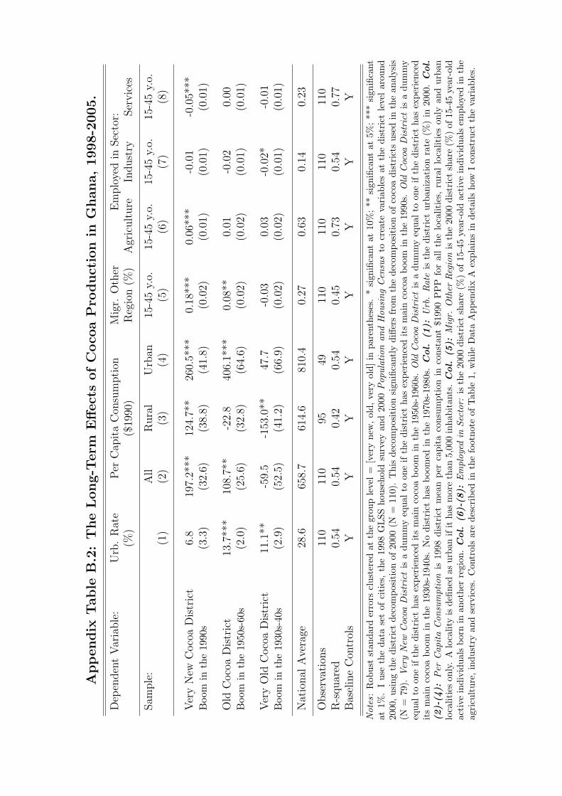
Ap

pen

dix

Tab

leB

.2:

Th

eL

on

g-T

erm

Eff

ect

sof

Coco

aP

rod

uct

ion

inG

han

a,

1998-2

005.

Dep

enden

tV

aria

ble

:U

rb.

Rat

eP

erC

apit

aC

onsu

mpti

onM

igr.

Oth

erE

mplo

yed

inSec

tor:

(%)

($19

90)

Reg

ion

(%)

Agr

icult

ure

Indust

rySer

vic

es

Sam

ple

:A

llR

ura

lU

rban

15-4

5y.

o.15

-45

y.o.

15-4

5y.

o.15

-45

y.o.

(1)

(2)

(3)

(4)

(5)

(6)

(7)

(8)

Ver

yN

ewC

oco

aD

istr

ict

6.8

197.

2***

124.

7**

260.

5***

0.18

***

0.06

***

-0.0

1-0

.05*

**B

oom

inth

e19

90s

(3.3

)(3

2.6)

(38.

8)(4

1.8)

(0.0

2)(0

.01)

(0.0

1)(0

.01)

Old

Coco

aD

istr

ict

13.7

***

108.

7**

-22.

840

6.1*

**0.

08**

0.01

-0.0

20.

00B

oom

inth

e19

50s-

60s

(2.0

)(2

5.6)

(32.

8)(6

4.6)

(0.0

2)(0

.02)

(0.0

1)(0

.01)

Ver

yO

ldC

oco

aD

istr

ict

11.1

**-5

9.5

-153

.0**

47.7

-0.0

30.

03-0

.02*

-0.0

1B

oom

inth

e19

30s-

40s

(2.9

)(5

2.5)

(41.

2)(6

6.9)

(0.0

2)(0

.02)

(0.0

1)(0

.01)

Nat

ional

Ave

rage

28.6

658.

761

4.6

810.

40.

270.

630.

140.

23

Obse

rvat

ions

110

110

9549

110

110

110

110

R-s

quar

ed0.

540.

540.

420.

540.

450.

730.

540.

77B

asel

ine

Con

trol

sY

YY

YY

YY

Y

Not

es:

Rob

ust

stan

dard

erro

rscl

uste

red

atth

egr

oup

leve

l=

[ver

yne

w,

old,

very

old]

inpa

rent

hese

s.*

sign

ifica

ntat

10%

;**

sign

ifica

ntat

5%;

***

sign

ifica

ntat

1%.

Ius

eth

eda

tase

tof

citi

es,

the

1998

GL

SSho

useh

old

surv

eyan

d20

00P

opul

atio

nan

dH

ousi

ngC

ensu

sto

crea

teva

riab

les

atth

edi

stri

ctle

vel

arou

nd20

00,u

sing

the

dist

rict

deco

mpo

siti

onof

2000

(N=

110)

.T

his

deco

mpo

siti

onsi

gnifi

cant

lydi

ffers

from

the

deco

mpo

siti

onof

coco

adi

stri

cts

used

inth

ean

alys

is(N

=79

).V

ery

New

Coc

oaD

istr

ict

isa

dum

my

equa

lto

one

ifth

edi

stri

ctha

sex

peri

ence

dit

sm

ain

coco

abo

omin

the

1990

s.O

ldC

ocoa

Dis

tric

tis

adu

mm

yeq

ual

toon

eif

the

dist

rict

has

expe

rien

ced

its

mai

nco

coa

boom

inth

e19

50s-

1960

s.O

ldC

ocoa

Dis

tric

tis

adu

mm

yeq

ual

toon

eif

the

dist

rict

has

expe

rien

ced

its

mai

nco

coa

boom

inth

e19

30s-

1940

s.N

odi

stri

ctha

sbo

omed

inth

e19

70s-

1980

s.Col.

(1):

Urb

.R

ate

isth

edi

stri

ctur

bani

zati

onra

te(%

)in

2000

.Col.

(2)-

(4):

Per

Cap

ita

Con

sum

ptio

nis

1998

dist

rict

mea

npe

rca

pita

cons

umpt

ion

inco

nsta

nt$1

990

PP

Pfo

ral

lth

elo

calit

ies,

rura

llo

calit

ies

only

and

urba

nlo

calit

ies

only

.A

loca

lity

isde

fined

asur

ban

ifit

has

mor

eth

an5,

000

inha

bita

nts.

Col.

(5):

Mig

r.O

ther

Reg

ion

isth

e20

00di

stri

ctsh

are

(%)

of15

-45

year

-old

acti

vein

divi

dual

sbo

rnin

anot

her

regi

on.Col.

(6)-

(8):

Em

ploy

edin

Sect

or:

isth

e20

00di

stri

ctsh

are

(%)

of15

-45

year

-old

acti

vein

divi

dual

sem

ploy

edin

the

agri

cult

ure,

indu

stry

and

serv

ices

.C

ontr

ols

are

desc

ribe

din

the

foot

note

ofT

able

1,w

hile

Dat

aA

ppen

dix

Aex

plai

nsin

deta

ilsho

wI

cons

truc

tth

eva

riab

les.

Ap

pen

dix

Tab

leB

.3:

Coco

aP

rod

uct

ion

an

dIn

frast

ruct

ure

Invest

ments

inG

han

a,

2000.

Dep

enden

tV

aria

ble

:Shar

eof

Inhab

itan

ts≤

10K

ms

Fro

m(%

)Shar

eof

Inhab

itan

tsD

ensi

tyof

Pav

edP

rim

ary

Sch

ool

Hea

lth

Cen

tre

Pos

tO

ffice

wit

hE

lect

rici

ty(%

)R

oads

(Met

ers/

Sq.K

m.)

Sam

ple

:R

ura

lU

rban

Rura

lU

rban

Rura

lU

rban

Rura

lU

rban

(1)

(2)

(3)

(4)

(5)

(6)

(7)

(8)

(9)

New

Coco

aD

istr

ict

0.01

**0.

00-0

.06*

**0.

01**

-0.0

3**

-0.0

3**

0.06

**0.

14**

*-4

.08

Boo

min

the

1990

s(0

.00)

(0.0

0)(0

.01)

(0.0

0)(0

.01)

(0.0

1)(0

.02)

(0.0

1)(4

.58)

Old

Coco

aD

istr

ict

0.02

**0.

000.

08**

0.00

0.16

***

0.06

**0.

06**

0.11

***

4.09

*B

oom

inth

e19

50s-

1960

s(0

.00)

(0.0

0)(0

.02)

(0.0

0)(0

.02)

(0.0

1)(0

.02)

(0.0

1)(1

.55)

Ver

yO

ldC

oco

aD

istr

ict

0.03

***

0.00

0.10

**0.

02*

0.19

**0.

05**

0.06

*0.

06**

*21

.8**

*B

oom

inth

e19

30s-

1940

s(0

.00)

(0.0

0)(0

.02)

(0.0

1)(0

.03)

(0.0

1)(0

.02)

(0.0

1)(1

.61)

Nat

ional

Ave

rage

0.98

0.99

0.77

0.98

0.57

0.94

0.16

0.61

34.8

Obse

rvat

ions

110

106

110

106

110

106

108

106

110

R-s

quar

ed0.

610.

990.

610.

580.

650.

380.

400.

340.

69B

asel

ine

Con

trol

sY

YY

YY

YY

YY

Not

es:

Rob

ust

stan

dard

erro

rscl

uste

red

atth

egr

oup

leve

l=

[ver

yne

w,

old,

very

old]

inpa

rent

hese

s.*

sign

ifica

ntat

10%

;**

sign

ifica

ntat

5%;

***

sign

ifica

ntat

1%.

Ius

eth

e20

00Fa

cilit

yC

ensu

san

dP

opul

atio

nan

dH

ousi

ngC

ensu

sto

crea

teva

riab

les

atth

edi

stri

ctle

vela

roun

d20

00,u

sing

the

dist

rict

deco

mpo

siti

onof

2000

(N=

110)

.T

his

deco

mpo

siti

onsi

gnifi

cant

lydi

ffers

from

the

deco

mpo

siti

onof

coco

adi

stri

cts

used

inth

ean

alys

is(N

=79

).V

ery

New

Coc

oaD

istr

ict

isa

dum

my

equa

lto

one

ifth

edi

stri

ctha

sex

peri

ence

dit

sm

ain

coco

abo

omin

the

1990

s.O

ldC

ocoa

Dis

tric

tis

adu

mm

yeq

ualt

oon

eif

the

dist

rict

has

expe

rien

ced

its

mai

nco

coa

boom

inth

e19

50s-

1960

s.O

ldC

ocoa

Dis

tric

tis

adu

mm

yeq

ual

toon

eif

the

dist

rict

has

expe

rien

ced

its

mai

nco

coa

boom

inth

e19

30s-

1940

s.N

odi

stri

ctha

sbo

omed

inth

e19

70s-

1980

s.Col.

(1)-

(6):

%sh

are

ofru

ral

orur

ban

inha

bita

nts

who

are

less

than

10km

from

apr

imar

ysc

hool

,he

alth

cent

rean

dpo

stoffi

cein

2000

.A

loca

lity

isde

fined

asur

ban

ifit

has

mor

eth

an5,

000

inha

bita

nts.Col.

(7)-

(8):

%sh

are

ofru

ral

orur

ban

inha

bita

nts

wit

hac

cess

toel

ectr

icit

yin

2000

.Col.

(9):

dist

rict

dens

ity

ofpa

ved

road

sm

eter

s/

sqkm

in20

00.

Con

trol

sar

ede

scri

bed

inth

efo

otno

teof

Tab

le1,

whi

leD

ata

App

endi

xA

expl

ains

inde

tails

how

Ico

nstr

uct

the

vari

able

s.