Why Do Loans Contain Covenants? Evidence fromLending Relationships∗

Robert Prilmeier†

November 21, 2011

Abstract

The use of financial covenants varies widely across loans. While existing theoretical papers

provide hypotheses as to why some loans have more financial covenants than others, the

empirical evidence on these theories is very limited. In this paper, I test these theories

comprehensively using a novel identification approach based on lending relationships. Using

a large sample of corporate loans, I find that borrowers trade off monitoring benefits with

covenant-created hold-up costs, such that the effect of lending relationship intensity on

the number of covenants included in a loan follows an inverted U shape. Consistent with

covenant tightness addressing information asymmetry concerns, tightness is relaxed over the

course of a relationship.

∗I would like to thank my dissertation committee, Rene Stulz (chair), Isil Erel, and Mike Weisbach, for valuablediscussions and suggestions. I am also grateful for helpful comments from Jack Bao, Andrea Beltratti, Jian Cai,Phil Davies, E. Han Kim, Rose Liao, Ulrike Malmendier, Bernadette Minton, Berk Sensoy, Jerome Taillard andseminar participants at the Ohio State University.†PhD candidate at the Ohio State University, Fisher College of Business, 700 Fisher Hall, 2100 Neil Avenue,

Columbus, OH 43210, prilmeier 1@fisher.osu.edu.

1

1 Introduction

Finance theory predicts that giving state-contingent control rights to creditors can enhance firm

value (Aghion and Bolton, 1992; Dewatripont and Tirole, 1994). Financial covenants provide

for such a shift of control rights outside of bankruptcy when borrower performance falls below

a predefined accounting threshold. Recent studies document that covenants play an important

role in protecting creditors’ rights and that the presence of covenants is associated with lower

interest rates.1 Despite their role in improving value, there is substantial variation in covenant

use across loans of the same credit quality. Why do some loans provide for more frequent control

shifts than others?

Any answer to this question requires a theory of why covenants should be part of an optimal

debt contract. Monitoring incentive theories argue that state-contingent control shifts overcome

free-rider problems among a firm’s creditors (Rajan and Winton, 1995; Park, 2000). When a

firm’s cash flows are pledged to multiple creditors, it becomes difficult to implement monitoring

since other creditors will free-ride on the monitor. A covenant breach allows the lender to

renegotiate her debt ahead of other creditors, but only if she can prove that the covenant has

indeed been violated. Thus, her payoff becomes contingent on monitoring, which increases her

incentive to monitor. However, covenants can be costly because they allow lenders to hold

up borrowers and extract rents (Garleanu and Zwiebel, 2009). In addition, covenants protect

against moral hazard (Smith and Warner, 1979) and information asymmetries between the

borrower and the lender (Garleanu and Zwiebel, 2009).

To identify the way in which each of these effects impacts covenant use, I rely on the fact

that these theories offer different predictions about how covenant use should vary in a lending

relationship. Monitoring incentive theories predict that covenants should be given to the lender

with the lowest monitoring costs. Consequently, to the extent that monitoring costs decline in

a lending relationship, covenant use should increase. In particular, I argue that covenant use

should increase in relationship intensity at a decreasing rate because monitoring costs should fall

more strongly at the beginning of a lending relationship when the lender starts learning firm-

specific information. At the same time, state-contingent hold-up opportunities should increase

in relationship intensity at an increasing rate. As long as the current lender is not the one

1See Bradley and Roberts (2004), Chava and Roberts (2008), Roberts and Sufi (2009a), Nini et al. (2009,2010), Reisel (2010).

2

that has the most intensive relationship with the borrower, she will be unable to hold up the

borrower in case of a covenant violation since the borrower has access to another, potentially

better informed, lender. However, once a lender has become the best informed lender, her

state-contingent hold-up opportunities will increase in her information distance towards other

lenders. Taken together, these arguments predict that covenant use will increase in relationship

intensity at first, but then decrease again after a certain point.

The information asymmetry theory of covenant use generates an alternative prediction. To

the extent that lending relationships reduce information asymmetries about the potential for

wealth transfers from creditors to shareholders, this theory predicts a monotonically declining

need for covenants in a lending relationship.

I test these explanations for covenant use with a sample of 7,923 loans taken from the

DealScan database. I measure relationship intensity as the proportion of the firm’s borrowings

over the previous five years that have been arranged by the same lead arranger.2 I test the effect

of relationship intensity on covenant intensity, defined as the number of financial covenants

attached to a loan. Consistent with a trade-off between the incentive benefits and the hold-

up costs of using covenants to implement monitoring, I find that financial covenant intensity

increases with relationship intensity for low levels of relationship intensity, but decreases as the

relationship becomes more and more exclusive. These results are robust to alternative measures

of financial covenant intensity and relationship intensity.

Further, I investigate the effect of variation in the borrower’s bargaining power and the

lender’s stake in the loan. I argue that the decrease in covenant intensity in exclusive lending

relationships should be stronger for borrowers with better access to the public debt market.

These borrowers should enjoy higher bargaining power when contracting the loan, but not

after a covenant violation has occurred since public bondholders are likely to be even more

uninformed about the nature of the violation than any potential bank lenders. The evidence

supports this hypothesis. In addition, in a syndicated loan, all loan participants are entitled

to the same covenants. Therefore, covenant intensity does not prevent loan participants or

multiple lead arrangers for the same loan from free-riding on each other. If covenants are used

as a monitoring incentive, they should perform this role more effectively for sole lender loans or

2In loan syndication, the lead arranger (typically a bank) acts as an intermediary between the borrower andthe participant lenders and is responsible for performing the monitoring function (Ivashina, 2009).

3

loans with only one lead arranger. Indeed, I find that covenant use increases more strongly in

relationship intensity for such loans. Ex post competition from participant lenders or other lead

arrangers in the loan syndicate at the time of a covenant violation might alleviate the covenant-

created hold-up problem, provided that these lenders also learn about the firm’s prospects. I

find some evidence that the decrease in covenant intensity is concentrated in loans with one lead

arranger. I do not find evidence that covenant intensity is driven by a reduction in information

asymmetries between the borrower and the relationship lender.

The choice to borrow from a relationship lender is likely endogenous. To rule out that the

results are driven by selection effects, I employ three different strategies. First, I investigate

the relationship effect on loan contract terms to which the monitoring incentive and covenant-

created hold-up theories do not apply. I do not find an inverted U effect of relationship intensity

on these contract terms. In addition, I use propensity score matching (PSM) methods and

instrumental variables (IV) estimation. The instruments include the distance between the

borrower and the lead arranger as well as an indicator that both parties are located in the

same state, both of which should affect relationship formation. Moreover, I use the age of a

firm’s industry and the size of the median firm in the same industry to obtain an unconditional

expectation of relationship intensity. The results from the PSM and IV methods are consistent

with a causal effect of relationship intensity on covenant intensity.

Loan contracts not only involve a choice of how many covenants are included in the loan,

but also how tight they are. I define covenant tightness as the probability that the loan’s

most restrictive covenant will be violated. Predictions for covenant tightness are not necessarily

the same as for covenant intensity. In the model of Rajan and Winton (1995), the covenant

incentivizes the lender to monitor if it gives her control in bad states of nature, but it need not

be particularly tight. Since syndicated loan covenants are quite tight in general (Chava and

Roberts, 2008), monitoring incentive considerations may not induce variation in tightness. In

addition, while the average covenant may subject the borrower to state-contingent hold-up, the

violation of a very tight covenant is unlikely to be taken as a negative signal by outside lenders.

Demiroglu and James (2010) document that the violation of a tight covenant has little impact

on the borrower. I find that covenant tightness decreases in relationship intensity, and more so

when a reduction in information asymmetries is likely to be important.

4

My paper contributes to the growing literature on why debt contains covenants. Previous

work shows that covenants are used to mitigate agency costs and to flexibly monitor borrower

performance.3 However, the empirical literature thus far provides little evidence on the theory

that covenants are used as an incentive to monitor. In a recent study, Drucker and Puri (2009)

document that loans sold on the secondary markets contain more covenants, consistent with both

information asymmetry and monitoring incentive theories. The key innovation in this paper is

that it analyzes a situation – a lending relationship – where monitoring incentive theories and

information asymmetry stories generate different empirical predictions. This setup enables me

to provide direct evidence that covenant-created monitoring incentives matter.

The paper also contributes to the large literature on lending relationships. While this litera-

ture has traditionally focused on small, unlisted firms, several recent papers investigate lending

relationship effects on publicly listed borrowers. Bharath et al. (2011) find that relationships

reduce the cost of borrowing for listed firms. Schenone (2010) documents that unlisted borrow-

ers in exclusive relationships suffer ex ante hold-up costs in the form of larger yield spreads,

while listed borrowers do not. In this paper, I find that listed borrowers do care about state-

contingent hold-up and structure their loans to trade off this cost with the monitoring benefits

of covenants. This result is consistent with Murfin (2010) and Wardlaw (2010), who show that

relationship borrowers are more strongly affected by a bank’s tightening of credit standards

after the bank suffers defaults on other loans. However, in my paper the state contingency

arises at the borrower level rather than the bank level. Finally, I provide further evidence that

covenant intensity and covenant tightness are used in different ways, consistent with Demiroglu

and James (2010) who find that covenant tightness contains private information about the firm’s

prospects, but covenant intensity does not.

The remainder of this paper is structured as follows. Section 2 provides an institutional

background on financial covenants and describes the predictions from finance theory. Section

3 details the data collection process. Section 4 discusses the results for covenant intensity, and

section 5 addresses endogeneity concerns. Section 6 presents the results for covenant tightness,

section 7 performs additional robustness checks, and section 8 concludes.

3See, for example, Billett et al. (2007), Chava et al. (2010), Miller and Reisel (2011), Qi and Wald (2008),and Qi et al. (2011), in addition to the papers mentioned earlier.

5

2 Institutional background and theoretical framework

2.1 Financial covenants as a monitoring device

Financial covenants require the borrower to maintain certain accounting measures of financial

health, such as a minimum net worth or a maximum debt-to-EBITDA ratio. If the borrower

fails to comply with the covenant, he is deemed to be in technical default. This gives creditors

the right to accelerate the debt, i.e. demand immediate repayment. In practice, creditors rarely

exercise this right (Nini et al., 2010). Instead, covenant violations trigger a renegotiation process

in which the right to accelerate assigns a high amount of bargaining power to the creditors.

Recent studies document that creditors use this bargaining power to increase interest rates,

reduce the size of the credit line, or require additional collateral. However, they also push for

performance improvements and replacement of poorly performing CEOs.4 This distinction is

important because it means that covenants create benefits that accrue only to the lender with

covenants, but the lender’s monitoring of the covenants then leads to actions that benefit other

claimholders as well. A recent study by Moody’s Investors Service shows that recovery rates

for subordinated debtholders are substantially lower for defaulted covenant-lite loans than for

regular loans with covenants (5% vs. 30%).5

The following two cases provide good examples of how covenants work and how a lack

of covenants can erode value. In September 1998, Key Energy Services Inc (KES) entered a

revolving credit agreement with two term loans for $550 million with a loan syndicate led by

PNC Bank. The deal contained four covenants with a maximum debt/EBITDA covenant that

was set at slightly less than one quarterly standard deviation above KES’s debt/EBITDA ratio.

Between September and December 1998, the company’s stock lost roughly 50% in value, and the

company reported a net loss and a violation of its covenants. The loan syndicate responded by

reducing the credit available, increasing the interest rate, loosening some covenants, and adding

new covenants and restrictions. Ultimately, the firm recovered. In this case, creditors used their

control rights to reassess the company’s risk, reduce their exposure, and add restrictions to curb

moral hazard. While the firm might have recovered even without creditor intervention in this

4See Chava and Roberts (2008), Roberts and Sufi (2009a), Nini et al. (2009, 2010).5See Bullock, Nicole, “Private equity firms capture cov-lite benefits”, FT.com Financial Times, June 8,

2011. Interestingly, the covenant-lite lenders themselves did not have worse recoveries than lenders of loanswith covenants due to heavy collateralization, underscoring the unique monitoring role of covenants.

6

particular example, the above-mentioned findings of Nini et al. (2010) suggest that creditors do

play a positive role in a firm’s recovery after a covenant violation.

Creditors were less fortunate in the case of HomeBase Inc. This company entered a revolving

credit agreement for $250 million with a loan syndicate led by BankBoston. The loan contained

only one tangible net worth covenant that was loosely set. In fiscal year 2000, HomeBase

reported a net loss of $70 million, which did not trigger the covenant. On October 27, 2001,

$117.8 million were outstanding under the facility and the company reported a net loss of $188

million year-to-date, resulting in a covenant violation. On November 7, 2001, the company filed

for Chapter 11. Eventually it went into liquidation, and creditors lost 70 cents on the dollar.

This illustrates that when the covenant package is too weak, a violation may arrive too late for

the creditors to be able to protect themselves.

2.2 Monitoring incentive theories and state-contingent hold-up

When a firm’s cash flows are pledged to multiple claimholders, it becomes difficult to implement

monitoring since other claimholders will free-ride on the monitor. Rajan and Winton (1995) and

Park (2000) develop models that show how covenants can provide a solution to this problem. A

covenant breach allows the lender to renegotiate her debt ahead of other claimholders, but only

if she can prove that the covenant has indeed been violated. This makes her payoff contingent

on monitoring, which increases her incentive to monitor. In the model of Rajan and Winton

(1995), the lender will monitor if the monitoring benefit she receives exceeds monitoring costs.

In Park’s model, the optimal debt structure involves delegating monitoring to the lender with

the lowest monitoring cost. This lender receives the most restrictive set of covenants. To the

extent that relationships lower monitoring costs, both models predict that covenant use should

increase in a lending relationship.

However, this increase is likely nonlinear since monitoring costs should fall at a decreasing

rate. At the beginning of a relationship, the lender needs to determine what data to request, how

to interpret it and so forth, and she needs to learn about the firm-specific market environment.

Covenants tend to be tailored to the borrower’s situation. The definition of an accounting

ratio such as e.g. the fixed charge coverage ratio varies widely across loans and often these

definitions contain rules about how specific projects of the firm should be taken into account.

7

This suggests that lenders need to exert effort to determine appropriate definitions. In addition,

firm-specific information needs to be acquired in order to interpret covenant violations. When

making a second loan, the lender will have learned much of this information, so monitoring

costs will be lower. After several repeated interactions, monitoring costs should stabilize such

that subsequent interactions yield only minor or no cost reductions. This argument suggests

that covenant use due to monitoring incentives should rise most sharply at the beginning of a

lending relationship. Figure 1a illustrates this prediction.

Covenants come at a cost, however, since the imperfect correlation between accounting ratios

and financial health leads to uncertainty about the meaning of a covenant violation. On average,

covenant violators will have worse financial health than non-violators, but many violators are not

in serious trouble.6 Due to ongoing monitoring, relationship lenders are likely to be better able

to assess the information content of the covenant violation than uninformed lenders. Outside

lenders will tend to pool the firm with the set of all violators, which allows inside lenders to

extract rents from borrowers with good future prospects who violated a covenant due to a

random negative realization in an accounting ratio. Thus, covenants can create a potential for

state-contingent hold-up, which would not exist had the covenant not been written into the

contract. If the borrower foresees this problem when entering into the loan agreement, one

would expect him to negotiate for fewer restrictive covenants to be included in the contract.

Again, this effect is likely to increase nonlinearly in relationship intensity as shown in figure

1b. As long as some other lender has a more intensive relationship with the borrower than

the current lender, state-contingent hold-up by the current lender is unlikely since the other

lender should be able to correctly assess the violation. As the lending relationship becomes

increasingly exclusive, however, the information advantage of the current lender over potential

outside lenders becomes increasingly large. Hence, concerns about state-contingent hold-up

should play little role when relationship intensity is low, but become increasingly stronger as the

lending relationship moves towards exclusivity. Together, the countervailing forces of covenant

costs and benefits predict that the effect of relationship intensity on covenant use follows an

inverted U (see figure 1c). For low levels of relationship intensity, reductions in monitoring costs

6Nini et al. (2010) find that covenant violators have a one-year probability of exiting their sample due todistress of 6.4% compared to 2.6% for non-violators.

8

should lead to an increase in covenant use, while for high level of relationship intensity, concerns

about state-contingent hold-up should dominate and lead to a decrease in covenant use.

2.3 Information asymmetries

Garleanu and Zwiebel (2009) present an alternative theory on covenant use. They develop a

model that seeks to explain why covenants assign control to creditors remarkably often. In

their model, there is an information asymmetry between a lender and an entrepreneur about

the potential for future wealth transfers. They show that in this situation firm value can be

enhanced by giving the less informed party – the lender – strong decision rights. As the lender

collects information about the borrower, ex post renegotiation will be biased towards the lender

relinquishing these excessive rights. This model has two clear-cut implications in the context of

a lending relationship. First, to the extent that information asymmetries decline in a lending

relationship, covenants should become less restrictive. Second, this effect should be stronger for

more opaque borrowers where ex ante information asymmetries are likely to be larger.7

3 Data

I obtain data on syndicated and large sole lender loans from Loan Pricing Corporation’s

DealScan database. DealScan reports yield spreads, covenants, maturities and other loan char-

acteristics and accounts for a large proportion of the U.S. private loan market.8 Information on

financial covenants stems mainly from firms’ SEC filings making use of the fact that Regulation

S-K requires material contracts to be filed as exhibits (§229.601). Since firms started filing with

the SEC electronically in 1995, the sample ranges from January 1995 to December 2008.

The sample consists of U.S. currency denominated loans obtained by U.S. firms that are not

a member of the financial, utility, or public administration sectors. I merge this dataset with

the borrowers’ accounting data in Compustat for the fiscal year prior to loan inception using

a link file kindly provided by Michael Roberts and Sudheer Chava.9 Given that these publicly

7The point that the variation in covenant use enhances firm value is an important one. It implies that thebenefits of a reduction in information asymmetries in a lending relationship cannot be fully realized simply byaltering the interest rate. Rather, the interest rate would be a mechanism to redistribute the surplus generatedby a reduction in excessive renegotiation.

8According to Carey and Hrycay (1999), DealScan covers between 50 and 75% of all commercial loans (byvalue) in the U.S. in the early 1990s and coverage further increases thereafter.

9Details on the construction of this link file can be found in Chava and Roberts (2008).

9

listed firms tend to have a diverse set of claimholders, this sample provides a good setting to test

theories related to monitoring incentives. In addition, recent work has shown that information

asymmetries are an important determinant of contract terms (Bharath et al., 2011; Schenone,

2010) and syndicate structure (Sufi, 2007) for the firms covered in DealScan.

Borrowers’ S&P long-term issuer ratings are taken at the month before loan inception to

reflect the borrower’s risk assessment at the time the loan is made. After applying all filters,

the final sample for which the required information is available consists of 7,923 loans incurred

by 3,169 borrowers. Loans are reported in DealScan as packages (or deals), which contain one

or more facilities. Information such as yield spreads, loan amounts, and maturities are available

at the facility level, whereas covenants are reported at the package level. To avoid artificially

weighting covenant observations by the number of facilities in the package, I aggregate all data

to the package level.10

Numerous bank mergers and acquisitions occurred during the sample period. To account

for the M&A activity, I match the DealScan lenders to FDIC institution IDs (RSSD IDs) based

on name, geographical location and time. I perform this match at the individual bank level

rather than the bank holding company level on the theory that firm-specific information is

learned through direct interaction and possible transfer of this knowledge across individual

banks is subject to frictions. Using this match, the Federal Reserve’s National Information

Center allows me to track bank mergers over time and attribute an acquired bank’s relationships

to the surviving entity.

I measure both financial covenant and non-financial covenant intensity as count variables

that add one for each financial and non-financial covenant, respectively, as recorded in DealScan.

Table 1 details the various types of financial and non-financial covenants. Financial covenants

are grouped into six categories: debt to balance sheet, coverage, debt to cash flow, liquidity, net

worth, and EBITDA covenants. Debt to balance sheet and debt to cash flow covenants restrict

the maximum indebtedness the borrower is allowed to incur relative to the various balance sheet

and cash flow items detailed in table 1. Coverage, liquidity, net worth, and EBITDA covenants

all require the maintenance of certain minimum coverage or liquidity ratios or of a minimum

10One might wonder to what extent the results are influenced by firms incurring multiple loans within oneyear. It turns out that in the final sample, 91.6% of the firm-year combinations are unique, while for 7.7% of thefirm years there are two loans in the sample, and for 0.7% of the firm years there are three or four loans in thesample. Consequently, aggregating observations to firm-years does not change results.

10

net worth or EBITDA. Among financial covenants, coverage covenants are the most frequent,

with 79% of all loans containing at least one such covenant. Debt to cash flow covenants and

net worth covenants are included in 60% and 43% of the loans, respectively.

Non-financial covenants include sweep provisions, dividend restrictions and capital expen-

diture restrictions. Sweep provisions require the borrowing firm to repay part or all of the loan

prematurely if it takes certain actions. For example, if a loan carries an asset sales sweep, the

borrowing firm must use asset sale proceeds in excess of certain allowances to repay the loan.

Close to 80% of all loans have a dividend restriction, while about one fifth of the loans have a

capital expenditure restriction. Among the 38% of all loans that carry a sweep provision, the

majority has more than one such provision.11

The empirical predictions require measuring relationship intensity in a way that captures

both the lender’s prior experience with the borrower as well as the exclusiveness of the relation-

ship. I define the lender as the loan’s lead arranger since the lead arranger acts as an interme-

diary between the borrower and the participant lenders and is better informed (Ivashina, 2009;

Guerin, 2007). I designate as lead arrangers any lender for which the field “lead arranger credit”

is marked “Yes” in DealScan as well as the lenders of all sole lender loans. In addition, I search

the field “lender roles” and define the following roles as lead arrangers: agent, administrative

agent, arranger, lead bank. These definitions coincide with Bharath et al. (2011), who describe

these roles in more detail. I then identify all instances in DealScan where the borrower obtained

funding in the five years prior to the current loan (including loans that are not in the final

sample due to missing information) and measure relationship intensity as follows:12

Relation (Max Amt) = maxk

∑j Loan amountj ∗ I(k)∑

j Loan amountj, (1)

where I(k) indicates lead arranger k’s participation in loan j. In words, I determine relationship

intensity as the total amount of loans over the past five years for which the current lead arranger

11Note that data on non-financial covenants in DealScan is often missing, even when data on financial covenantsis available. Since the vast majority of DealScan’s covenant information comes from loan documents filed withthe SEC, whenever there is information on financial covenants, information on non-financial covenants should beavailable to LPC. Thus, I set non-financial covenants to zero if the information is missing, but data on financialcovenants is available. This method appears to be similar to practitioners’ approach (e.g. May and Verde (2006)).In any case, non-financial covenants are not the focus of this study.

12This measure is also used by Bharath et al. (2011) and Schenone (2010). Assuming that a lending relationshipends if borrower and lender have not had a lending contact within five years appears reasonable since 84% of allloans in the sample have a maturity of five years or less.

11

acted as a lead arranger divided by the total amount of all loans over the past five years.13 If

there are no loans in the previous five years, the measure is undefined. Thus, I require at

least one prior loan to be observable. If the current loan has more than one lead arranger, I

take the maximum of that ratio across all lead arrangers since the monitoring effort is likely

to be led by the lead arranger with the lowest monitoring cost. As an alternative, I consider a

relationship intensity measure that gives equal credit to each lead arranger involved in the loan

and calculates the sum of relationship intensities across lead arrangers:

Relation (Sum Amt) =∑k

∑j Loan amountj/Nj ∗ I(k)∑

j Loan amountj, (2)

where Nj indicates the number of lead arrangers participating in loan j. Relative to the Relation

(Max Amt) measure, this measure has the advantage that it equals one if and only if there is no

lender outside of the current syndicate who has ever acted as a lead arranger to the firm. The

disadvantage is that it is not clear why a lead arranger should experience a smaller reduction

in monitoring cost over time if there is another lead arranger present in the syndicate. In any

case, the two measures differ only if multiple lead arrangers are involved in any of the firm’s

loans.14 Consequently, they have a correlation of 0.957 and lead to very similar results.

Table 2 shows the number of loans available per firm for the final sample and for the sample

used to determine relationship intensity. The median firm has two loans in the final sample and

four loans in the sample used to determine relationship status. Thus, using all available loans

in DealScan to calculate relationship intensity is important if one wants to be able to detect any

nonlinear effect. Section 7 discusses the reasons why certain loans drop out of the final sample

and perform robustness checks to ensure that this does not affect results.

Table 3 presents univariate tests of differences in firm and loan characteristics conditional on

relationship intensity. Relationship intensity is categorized as “low” if Relation (Max Amt) is less

than 30%, “high” if it is more than 70%, and “medium” if it is in between. The results show that

financial covenant use increases by about 4% from the low to the medium category and decreases

13It should be noted that a substantial number of the observations in DealScan are renegotiations, ratherthan new loan originations (Roberts and Sufi, 2009b; Roberts, 2010). I assume that more frequent renegotiationimplies a higher relationship intensity. The distinction between originations and renegotiations is not materialfor this study, since I investigate the dynamics over the course of a lending relationship, rather than examiningan effect that is limited to loan originations.

14Among the loans in the sample, 74.4% have one lead arranger, 22.1% have two lead arrangers and 3.5% havemore than two lead arrangers.

12

by about 7% from the medium to the high category. The changes are highly statistically

significant. Covenant tightness declines in relationship intensity. Yield spread, non-financial

covenant use, and collateral requirements decrease in relationship intensity, whereas maturity

is largely unchanged. However, table 3 also shows that firm characteristics are correlated with

relationship intensity, with firms with high relationship intensities being larger, more likely to

be a member of the S&P 500, more likely to be rated, having better ratings, and having a lower

current ratio. Therefore, I now turn to multiple regressions.15

4 Multiple Regressions for Covenant Intensity

4.1 Baseline Tests

Since the number of financial covenants is a count variable, I test the effect of relationship

intensity on financial covenant intensity by estimating Poisson regressions. One way to allow

for the inverted U shape described in section 2 is to use a quadratic form:

log(FinCovi) = α1 + β1 Relationi + γ1 Relation2i + δ1 Controlsi + ε1,i , (3)

where FinCov is the number of financial covenants included in a deal and Relation is one of the

two relationship intensity measures. Since the linear and squared terms of relationship intensity

are highly correlated, one may be concerned that regression estimates are an artifact of this

correlation. Therefore, I focus on presenting results using a dummy variable specification:

log(FinCovi) = α2 + β2 LowRelationi + γ2 HighRelationi + δ2 Controlsi + ε2,i , (4)

where Low Relation and High Relation are dummy variables that equal one if relationship inten-

sity is below 30% and at least 70%, respectively. Consequently, loans with medium relationship

intensities become the base group, which allows testing for the existence of any U-shape. Con-

trols include various loan and firm characteristics as displayed in table 3 as well as industry

fixed effects at the one-digit SIC industry level, year fixed effects, and loan purpose and loan

15In unreported regressions, I confirm the negative effect of relationship intensity on spreads, collateral re-quirements, and maturity found by Bharath et al. (2011) and obtain very similar coefficients. Although dataavailability on financial covenants is not as extensive as for the terms they investigate, this similarity in resultslends support to the quality of my sample.

13

type fixed effects. If one deal contains two different types of loans, e.g. a revolver and a term

loan, then both these dummy variables equal one for that deal.16 As is customary in studies

using Compustat data, the top and bottom 1% of all financial ratios are winsorized to control

for outliers.17

Table 4 shows the results. The effect of relationship intensity on financial covenant inten-

sity appears to follow an inverted U-shape. For the quadratic specifications, the linear term

is significantly positive and the quadratic term significantly negative. For the dummy vari-

able specifications, both the low and high relationship dummies indicate a significantly lower

covenant intensity compared to loans with a medium relationship intensity. Table 4 also shows

that financial covenant use decreases in the size of the loan and in firm size. The coefficient

of leverage is positive as expected, but not significant. Covenant use increases in the number

of lenders participating in the loan, which mirrors the result in Drucker and Puri (2009) that

loans sold on the secondary market contain more covenants than loans that banks keep on their

balance sheet. Both the current ratio and the coverage ratio enter positively in the regression.

Many covenants are written on ratios related to these two. Such covenants may be more infor-

mative if these ratios are above a certain threshold.18 Firms with a worse credit rating or no

credit rating at all are subject to more covenants, while loans to members of the S&P 500 carry

fewer covenants.19

The relationship effect is economically significant. Figure 2 plots the effect of relationship

intensity on covenant intensity using the quadratic specification from regression (2) in table

4 and a stepwise dummy variable specification using the same controls (not reported in the

table). Financial covenant intensity increases by about 8% from low to medium relationship

intensity and decreases by about 4% from medium to high relationship intensity. These changes

are equivalent to the effect of a change in the rating by two to three notches and by one to two

notches, respectively. For further comparison, a one standard deviation increase in leverage is

16I exclude loan purpose and loan type dummies that have fewer than ten nonzero observations in the sample.17These winsorizations have an effect on the coefficients of some of these ratios, but they do not change the

results regarding the relationship effect.18Current ratio covenants typically stipulate a minimum ratio of 1.0 or higher, while interest coverage ratio

covenants typically stipulate a minimum of 1.25 or higher. If one excludes loans from borrowers whose ratios arebelow one of these thresholds, the current ratio and coverage ratio are no longer significant in the regressions.

19A potential problem with Poisson models is over- or underdispersion of the data relative to the model.Calculating the deviance for the models in table 4 and dividing by the degrees of freedom gives a value of 0.324,which is smaller than one and hence suggests that underdispersion is present. Standard errors scaled by thesquare root of the deviance-based dispersion are slightly smaller than standard errors clustered at the firm level.

14

associated with an increase in financial covenant intensity by about 1% (or 2% if one removes

the rating variable from the regression) and a one standard deviation increase in the log of

assets leads to a decrease by about 4% (or 7% after removing the S&P 500 dummy). The

relationship effect on covenants is also similar in size to the effect on other loan terms. For

example, Bharath et al. (2011) find that a change in relationship intensity from 0% to 100%

leads to a decrease in the all-in-spread drawn by 5% (evaluated at their sample average). The

stepwise specification in figure 2 also shows that the relationship intensity thresholds of 30%

and 70% used for the dummy variable specification in regression (3), while somewhat arbitrary,

capture the curve quite well. A variety of alternative cutoffs exists that would yield similar or

stronger results.

4.2 Bargaining Power and Syndicate Structure

An important way of distinguishing state-contingent hold-up from information asymmetry ef-

fects is to consider the borrower’s bargaining power. If covenant violations provide an exclusive

lender with an opportunity to hold up the borrower, borrowers should seek to avoid this hold-

up potential by writing fewer covenants into their loans. However, their effectiveness at doing

so is likely to depend on their bargaining power when contracting the loan. A borrower with

better access to outside capital should be better able to adjust his loan contracts for the state-

contingent hold-up problem. Because borrowers with access to outside capital markets tend to

be more transparent, an information asymmetry story would predict the opposite: The decrease

in covenant intensity for high relationship intensities should be more pronounced for opaque

firms that do not have access to outside capital markets. I use the existence of an S&P long-

term issuer rating as well as a firm’s access to the commercial paper market (as evidenced by

a short-term rating of A-2 or better (Murfin, 2010)) as proxies for the firm’s access to public

debt markets.20

Columns 1 and 5 of table 5 show that the decrease in covenant intensity for firms in exclusive

relationships is concentrated in rated firms. Among rated firms, covenant intensity is between

6% and 7% lower for borrowers in exclusive relationships as compared to borrowers in medium

20One might wonder whether the state-contingent hold-up problem itself is smaller for rated borrowers. How-ever, note that investors on the public debt market are most likely even more uninformed than potential outsidebank lenders. Thus, access to the public debt market provides the borrower with bargaining power ex ante, butnot necessarily after a covenant violation has occurred. In any case, this would hurt my identification strategy.

15

intensity relationships.21 Figure 3 plots the difference in the relationship effect for rated vs.

unrated firms using a quadratic specification (not reported in table 5). For rated firms, covenant

intensity increases until a relationship intensity of about 53% and decreases strongly thereafter,

while for unrated firms covenant intensity increases until a relationship intensity of about 60%

and remains relatively constant for higher relationship intensities.22 Columns 2 and 6 of table 5

show that the interaction between high relationship intensity and access to the commercial paper

market has similar coefficients to the interaction with being rated, but is at best marginally

significant statistically. Consequently, it appears that having any rating is more important than

having a rating that indicates a particularly high credit quality.

I next turn to the impact of syndicate structure on the relationship effect. This matters

for two reasons. First, an increase in the number of participants limits the extent to which

monitoring benefits accrue to the lead arranger. In the Rajan and Winton (1995) model,

covenants incentivize the lender to monitor because a covenant violation allows her to demand

early repayment or adjustments to the contract without having to share these benefits with other

creditors. In a borrowing syndicate with multiple loan participants or lead arrangers, every

lender is treated equally in the event of a covenant breach, which reintroduces the free-rider

problem. Consequently, if monitoring incentives motivate the inclusion of financial covenants in

contracts with relationship lenders, the increase in covenant use from low to medium relationship

intensities should be stronger for sole lender loans than for syndicated loans and it should be

stronger for loans with one lead arranger than for loans with multiple lead arrangers. Second,

to the extent that other loan participants, or especially, co-lead arrangers become informed

about the borrower, the potential to hold up a borrower when he violates a covenant may be

reduced. If a hold-up attempt occurs, an informed competitor within the syndicate could offer

the borrower better terms and win his business. This incentive to deviate may reduce the need

to decrease covenant intensity for high relationship intensities.

21This effect does not appear to be driven by the fact that controlling for the level of the rating helps theregression model better measure credit quality for rated borrowers than for unrated borrowers. When dropping theordinal rating variable and thus leveling the playing field, coefficients on the interaction terms remain qualitativelyand quantitatively similar.

22Ai and Norton (2003) point out that the interpretation of interaction terms can be difficult in nonlinearmodels. This problem does not apply here since the Poisson model is linear in the log of the covenant count,which makes analyzing percentage changes in incidence rates straightforward. Couching the discussion in termsof percentage changes appears reasonable since financial covenants are written on correlated accounting ratios.On average, adding a second covenant should increase restrictiveness more than adding a tenth covenant.

16

Columns 3 and 7 of table 5 show the increase in covenant intensity with an increase from

low to medium relationship intensity is stronger for sole lender loans. According to columns

4 and 8, the inverted U curve is flatter for loans with multiple lead arrangers, although the

difference is significant only for the relationship measure that gives 1/N credit to each of the N

lead arrangers. These results are consistent with both covenant-created monitoring incentives

and within-syndicate competition among lead arrangers.

4.3 The Borrower’s Information Opacity

As described in section 2, a reduction in information asymmetries over the course of a lending

relationship might result in a lower need for giving the lender decision rights through financial

covenants. I now test whether this is the case and whether the reduction in covenant intensity

for exclusive relationships is driven by such an effect. Proxies for information opacity include

dummy variables indicating whether the borrower’s total assets are below the sample median

during the start year of the loan, whether the borrower’s stock is a member of the S&P 500

index, whether the borrower is a high tech firm (defined as in Loughran and Ritter (2004)),

whether the number of analysts following the borrower’s stock is below the sample median for

that year, whether the dispersion of analyst forecasts for the borrower’s earnings per share is

above the median, and whether the borrower is listed on NASDAQ as opposed to NYSE or

Amex. It should be noted that many of these proxies are negatively related to a firm’s access to

capital markets and, hence, its ex ante bargaining power. To the extent that bargaining power

matters more than information asymmetries, one would expect results to mirror those of the

previous section. Although opaque firms might be easier to hold up after a covenant violation,

they are likely to lack the bargaining power to adapt the loan contract to this hold up potential

in the first place.

Table 6 presents results using the Relation (Max Amt) measure. Results using the Relation

(Sum Amt) measure are qualitatively and quantitatively similar and are omitted for brevity.

Table 6 shows that the evidence is inconsistent with a lower need for covenants due to a reduction

of information asymmetries over the course of a relationship. The downward sloping part of the

inverted U is stronger for large borrowers, borrowers with a large analyst following and borrowers

whose stock is part of the S&P 500. The first two of these interactions are statistically significant

17

at the 5% level, while the interaction with S&P 500 membership is marginally significant at

the 10% level. There is no difference for high tech vs. other firms, NASDAQ vs. NYSE/Amex

firms, or firms with high vs. low dispersion of analyst forecasts, proxies that arguably are less

related to capital markets access and more related to pure information asymmetries.23

Taken together, the results presented thus far support the theory that covenant choice

involves a trade-off between monitoring incentives and state-contingent hold-up. The evidence

is inconsistent with covenant intensity being driven by a reduction in information asymmetry

between the borrower and the relationship lender since I find that the reduction in covenant

intensity in exclusive relationships is driven by large, rated firms rather than small, opaque

firms. The evidence is also inconsistent with the idea that the initial increase in covenant

intensity may be driven by hold-up when contracting the loan (Rajan, 1992). Under this story,

the initial increase should be concentrated in opaque borrowers, but the evidence shows it is

also present (or stronger, if anything) for large and rated firms which succeed in negotiating

a lower financial covenant intensity even in exclusive relationships. Another story is that the

increase in covenant use is not due to monitoring incentives, but due to the lead arranger’s

monitoring commitment towards participant lenders. This story predicts a stronger upward

slope for syndicated loans than for sole lender loans, which is the opposite of what I find.

5 Endogeneity of relationship choice

The choice of forming, developing, and breaking a banking relationship is likely to be endoge-

nous. Perhaps firms that do not form relationships differ from firms that have relationships

with several banks and firms that have an exclusive relationship in ways that explain the in-

verted U-effect documented thus far. Note that any such endogeneity story would also have

to account for the finding that the reduction in covenant intensity is concentrated in rated

firms that have higher ex ante bargaining power. While it seems difficult to construct such a

story, this section employs three different ways to test whether results are driven by selection

on observable or unobservable firm characteristics. The first strategy analyzes loan terms to

which neither the monitoring incentive argument nor the covenant-created hold-up argument

23Firm size, being rated, and the propensity to use multiple lead arrangers are all correlated. When I estimateregressions with interaction terms for all three, results for the interaction terms with having a rating and withusing multiple lead arrangers are consistent with the results shown earlier, while the size interaction is notsignificant.

18

applies. There should not be an inverted U-effect for these loan terms. The second strategy

discusses relationship effects estimated by propensity score matching methods and the third

uses an instrumental variables approach.

5.1 Relationship effects on yield spreads and non-financial covenants

Yield spreads do not offer the state-contingent control feature embedded in financial covenants.

For this reason, neither the monitoring incentive theory nor state-contingent hold-up concerns

are applicable to yield spreads. However, to the extent that relationships mitigate information

asymmetries between the borrower and the relationship lender, yield spreads should decrease in

relationship intensity. Given these theories, finding an inverted U-effect of relationship intensity

on yield spreads would call into question the conclusions drawn above. It would mean that the

inverted U could be driven by sample selection effects or, since yield spreads are related to

credit risk, by failing to control for an important risk factor. Bharath et al. (2011) study the

effect of relationship intensity on yield spreads for a sample of borrowers contained in DealScan

and find that yield spreads decrease in relationship intensity, and more so for informationally

opaque borrowers, consistent with the information asymmetry theories. Nevertheless, it appears

worthwhile to perform a similar analysis for my sample since their sample selection criteria differ

from mine24 and since they do not allow for nonlinearity of the relationship effect.

In table 7, I regress the all-in spread drawn provided by DealScan on relationship intensity

and the same controls that are used in the previous regressions. The relationship intensity

measure used is Relation (Max Amt) as defined in equation 1, but conclusions are not affected

by using the Relation (Sum Amt) measure. Column (1) shows that yield spreads decrease in

relationship intensity. Column (2) allows for an inverted U shape, but does not find such an

effect. I further analyze the effect of the relationship asymmetry and bargaining power proxies.

Columns (3) and (4) show that the decrease of yield spreads in relationship intensity is driven

by unrated and small borrowers who are likely more opaque. The result is exactly the opposite

of what I find for financial covenants. This finding reduces the likelihood that the documented

decrease of financial covenant intensity in exclusive relationships for large, rated borrowers is due

to unobserved risk. Columns (5) and (6) show that the relationship effect on yield spreads is not

24Most notably, I require the availability of information on financial covenant intensity and I analyze loans atthe deal level, while they focus on the facility level.

19

significantly larger for borrowers listed on NASDAQ, but it is significantly larger for borrowers

with higher dispersion of analysts’ earnings forecasts. Importantly, column (7) does not reject

the hypothesis that the effect of relationship intensity on yield spreads for loans with multiple

lead arrangers is the same as the effect for loans with one lead arranger. This result supports

the interpretation that the weaker inverted U-shape for loans with multiple lead arrangers is

due to loan-level financial covenants’ inability to overcome monitoring incentive problems and

due to within-syndicate competition at the covenant violation point. It is inconsistent with the

argument that loans with multiple lead arrangers are simply transactional loans.

A further test in table 7 concerns non-financial covenants. While financial covenants define

certain financial health criteria that the borrower might fail to meet for a plethora of reasons,

non-financial covenants restrict specific actions that typically involve some form of moral haz-

ard, such as capital expenditures, dividend payouts, and asset sales. Financial covenants are

thus written on quantities that are more volatile and less directly controllable by managers than

those that non-financial covenants contract on (Kahan and Tuckman, 1993). This means that

financial covenants require a larger effort on the part of the monitor to evaluate the implica-

tions of a violation and that they are less transparent to uninformed lenders. Consequently,

monitoring incentive and violation hold-up considerations should be more pronounced for finan-

cial covenants, whereas non-financial covenants should be more strongly related to information

asymmetries.

Columns (8) and (9) in table 7 test this prediction. Allowing for a linear term shows a

significantly negative effect of relationship intensity on non-financial covenants. When allowing

for non-linearity, there is no evidence of an inverted U-shape for non-financial covenants. The

difference between medium and low relationship intensity loans is insignificant,25 whereas high

relationship intensity loans carry significantly fewer non-financial covenants. This result is

again inconsistent with the interpretation that the inverted U-effect of relationship intensity on

financial covenant use is driven by a background factor that affects the choice of loan terms in

general.

25While the sign is negative using the Relation (Max Amt) measure, it is positive and still insignificant usingthe Relation (Sum Amt) measure.

20

5.2 Propensity score matching

While the results using yield spreads and non-financial covenants are instructive and corroborate

the interpretation of the results presented in section 4, I now turn to direct strategies for

accounting for endogeneity. Ideally, one would like to randomly assign firms to groups that are

treated with either low, medium, or high relationship intensity and then observe their covenant

choices. In reality, however, firms are not assigned to treatment groups at random, and one

cannot observe what outcome a firm choosing a relationship loan would have experienced had

it chosen a non-relationship loan. However, for each firm that receives treatment, one can

try to find untreated firms that ex ante had the same likelihood to receive treatment and

estimate the average treatment effect on the treated (ATT) as the average of the difference

in financial covenant intensity between the matches. This can be done using propensity score

matching (PSM) as described in Rosenbaum and Rubin (1983) and Heckman et al. (1997, 1998).

Assuming that all factors affecting selection into treatment groups are observable, the resulting

estimate of the ATT is unbiased. Selection on unobservables, however, cannot be cured with

PSM and requires the use of an instrumental variables approach (see section 5.3). I implement

the PSM technique using the following steps.

First, I estimate each firm’s probability to be assigned to the low, medium, or high relation-

ship intensity group using an ordered probit model where the dependent variable equals one for

low, two for medium, and three for high relationship intensity, respectively. The ordered probit

model uses firm and loan characteristics from table 4 with year, industry, loan purpose and loan

type fixed effects as independent variables. I exclude the maturity of the loan and syndicate

size from the regression to address concerns that these may be endogenous themselves. Results

including these variables are qualitatively and quantitatively similar. The ordered probit model

yields three propensity scores – one for each relationship category.

Next, I estimate the ATT for medium relationship borrowers by matching each borrower

with medium relationship intensity to a set of borrowers with low relationship intensity based

on each borrower’s propensity to be treated with medium relationship intensity. In the same

fashion, the ATT for high relationship intensity borrowers is obtained by matching them with

medium relationship intensity borrowers based on the propensity to be in the high intensity

group. There are many ways to implement the matching estimator. For increased comparability

21

and transparency, I use the same estimators that Bharath et al. (2011) use.26 Nearest neighbor

estimators calculate the difference in financial covenant intensity between each treated loan and

the arithmetic average for the n loans in the untreated group with the closest propensity scores.

Following Bharath et al. (2011), I report results using n = 10 and n = 50. Kernel estimators

construct a counterfactual using a weighted average of financial covenant intensities for loans of

untreated firms. Weights decrease in the propensity score difference between the treated and the

untreated firms. The Gaussian kernel uses all untreated observations as matches, but weights

decrease faster the lower the bandwidth chosen to estimate the kernel. The Epanechnikov kernel

only uses untreated observations within the propensity score bandwidth. I employ a bandwidth

of 0.01. For the nearest neighbor matching, I estimate standard errors using the Abadie-

Imbens (2006) variance estimator. Standard errors for the kernel estimators are obtained from

bootstrapping with 1,000 replications.27

Table 8 shows the results for the PSM technique. Column (1) matches all medium rela-

tionship intensity loans with low relationship intensity loans and finds an ATT for financial

covenant intensity of about 0.13, or 5.1% relative to the sample average financial covenant in-

tensity of 2.54. This effect is slightly smaller than in the Poisson model, but highly statistically

significant. Column (4) matches all high relationship intensity loans to medium relationship

intensity loans, yielding a statistically significant ATT of about -0.09, or -3.5% relative to the

sample average, in line with the results from the Poisson model.

As Bharath et al. (2011) point out, there are two distinct groups of non-relationship borrow-

ers: those that never form relationships and those that just broke up an existing relationship

to borrow from a non-relationship lender. These groups may differ from each other in financial

covenant use, e.g. because borrowers break up relationships when a new lender offers them par-

ticularly favorable contract terms or, to the contrary, because the new lender needs to guard

against an adverse selection problem (Detragiache et al., 2000). Following Bharath et al. (2011),

26I implement all estimators using the Stata module PSMATCH2 provided by Leuven and Sianesi (2003).27Estimating standard errors for PSM poses some challenges. Abadie and Imbens (2008) show that the boot-

strap is not valid for nearest neighbor matching estimators due to a lack of smoothness. The variance estimator inAbadie and Imbens (2006) is asymptotically consistent assuming that propensity scores are known. In practice,however, propensity scores are estimated. Interestingly, Abadie and Imbens (2009) show for the variance of theaverage treatment effect (ATE) that adjusting for the estimation of propensity scores in the first step reducesthe asymptotic variance of the estimator. While it is not clear whether this finding also applies to the varianceof the ATT reported here, note that results for the ATE are virtually identical. To my knowledge, it is notclear whether the kernel estimators are smooth enough for the bootstrap to be valid. However, conclusions areunaffected by instead using the unconditional variance estimator provided in Lechner (2001).

22

I split the sample of low relationship intensity loans into two groups. The first group, which

becomes the untreated group in column (2) of table 8, consists of loans where the previous loan

had a relationship intensity larger than zero, but the current loan is a non-relationship loan,

thus breaking up an existing relationship. The second group, used as the untreated group in

column (3) of table 8, consists of loans that do not represent such a break up of an existing

relationship.28 It turns out that the increase in financial covenant intensity when moving from

low to medium relationship intensity is statistically significant regardless of comparison group,

although coefficients are somewhat larger when using firms that just broke up a relationship.

In a similar fashion, high relationship intensity borrowers can be distinguished into two

groups: those that always borrow from the same lead arranger and those that have at least

once in the past five years borrowed from some other lead arranger. It may be the case that the

first group is completely locked into their relationship, whereas the second group has the ability

to borrow from other lead arrangers, but chooses not to do so. Columns (5) and (6) address

this concern by restricting the treatment group to loans with a relationship intensity of exactly

one (column (5)), and a relationship intensity of more than 0.7, but less than one (column (6)).

As table 8 shows, this distinction does not matter. Coefficients are highly similar across the

two columns and the high relationship intensity effect is statistically significant in both.

5.3 Instrumental variables

Selection into a particular relationship status may be driven by unobservable factors such as

the firm’s and lender’s private information about the future prospects of the firm. Perhaps

firms with good unobservable credit quality tend to either borrow only transactional loans

(never forming a relationship) or focus on a relationship with one bank, while firms with poor

unobservable credit quality maintain relationships with more than one bank, thus creating the

observed inverted U-effect of relationship intensity. From a theoretical standpoint, it is not clear

why this should be the case. Nor is it consistent with the findings for yield spreads and the fact

that the inverted U is concentrated in loans obtained by rated firms, for which the information

on credit quality that is available to the researcher is more precise, if anything. Nevertheless,

such a concern can be addressed using instrumental variables (IV) estimation.

28If the previous loan has an undefined relationship status (because it is that borrower’s first loan in DealScan),this determination cannot be made and the loan is excluded from this part of the analysis.

23

The key to IV estimation is to find an instrument that is correlated with relationship status,

but has no effect on financial covenant intensity other than through relationship status. Since

this study uses two endogenous variables — low and high relationship intensity indicators —, at

least two instruments are needed to identify both endogenous variables. Bharath et al. (2011)

use the distance between the borrower and the lead arranger as an instrument. They argue

that geographical proximity fosters the gathering and processing of firm-specific information

and hence the formation of relationships, while not affecting loan terms per se.29 I use this

instrument as well. Historical addresses (city, state, and ZIP code) of borrowers’ headquarters

are obtained from the header of the corresponding 10-K filing using DirectEDGAR.30 Historical

lender addresses are from Call Reports and the National Information Center (NIC) of the

Federal Reserve System, which means that foreign lenders and non-bank lenders not covered by

the NIC are excluded from this analysis. I translate these data into geographical longitudes and

latitudes using the WebGIS application provided by the University of Southern California.31 I

then compute the log of one plus the spherical distance in miles between the borrower and the

lead arranger using the formula given in Dass and Massa (2011).32

A similar geographical argument can be made when the borrower and the lender are located

in the same state. In this case, the lender’s familiarity with the state-level economic, legal, and

political environment is likely to positively affect the processing of firm-specific information in a

relationship. At the same time, this proximity should not affect loan terms other than through

its effect on relationship formation. Hence, as a second instrument, I use an indicator variable

that equals one if at least one lead arranger is located in the same state as the borrower.

One concern with using two geographical instruments is that they may be too close in mean-

ing to be able to identify two distinct endogenous variables. For this reason, I also employ two

proxies for the unconditional expectation of relationship formation in the borrower’s industry.

Older and more established industries in which the average firm is relatively large are likely to

be more transparent and have access to a wider variety of capital sources. Consequently, bank-

ing relationships are less likely to be exclusive. I proxy for this using the median size of a firm

29See their paper for a discussion of the literature on geography and banking relationships.30I thank Burch Kealey for help with this data.31At the time of writing, this service is available at https://webgis.usc.edu/Default.aspx.32If the loan has more than one lead arranger, I take the distance between the borrower and the closest lead

arranger on the theory that the group of lead arrangers as a whole will be at least as informed as the mostwell-informed lead arranger.

24

in the borrower’s industry in the year prior to the loan start date as well as industry age, which

I define as 2008 minus the year of the earliest Compustat IPO date of any firm in the borrower’s

industry.33 These variables are likely to be correlated with relationship status of firms in the

borrower’s industry, but should not affect the loan terms of that particular borrower.34

Since the endogenous regressors represent a nonlinear function of the same variable, the

potential of instrument weakness is an immediate concern. To my knowledge, no procedure

is available to test for instrument weakness in the nonlinear generalized method of moments

setting, whereas tests and implications in the linear model are better understood (see Stock

et al. (2002)). For this reason, I implement a two-stage least squares (2SLS) estimation of

equation 4.35 Because Low Relation and High Relation are indicator variables, I follow the

recommendation in Wooldridge (2002) to first estimate a probability model for the relationship

dummies with the instruments described above and then use the predicted probabilities as the

actual instruments in the first stage of the 2SLS estimation.36 To account for the dependence

between the indicator variables, I choose an ordered probit model, but results using two separate

binary probit models are similar.

Results from the IV estimation are displayed in table 9.37 I present three models to assess

whether results depend on the choice of instruments. All four instruments are statistically

significant predictors of relationship intensity in the first stage ordered probit. The coefficients

on the instrumented relationship dummies remain negative and statistically significant.38 When

examining the IV results, it is apparent that the coefficients are very large compared to the

Poisson regressions. Two instrument weakness tests are reported: the Cragg-Donald F-statistic,

which assumes homoskedastic i.i.d. errors, and the Kleibergen-Paap rk F-statistic, which is

robust to firm-level clustering of standard errors. The Stock and Yogo (2005) critical value

33I group firms into industries using the Fama-French 38 industry classification.34The industry median size instrument is also used in Dass and Massa (2011).35To justify the application of the linear model to the log transformation of financial covenant intensity, I

re-estimate the results obtained thus far using ordinary least squares. The results are very similar qualitativelyand quantitatively to those presented in the previous sections.

36Note that this method is not the same as plugging the predicted probabilities into the second stage, whichwould amount to a case of “forbidden regression” (Wooldridge, 2002).

37Estimation uses the Stata module IVREG2 provided by Baum et al. (2010).38One might be concerned that geographical instruments harbor bias if a borrower that needs to be monitored

more closely cannot obtain a loan from a geographically distant lender. This would bias the IV estimationtowards finding a higher covenant use for higher relationship intensities. It would not explain an inverted U.Nevertheless, I estimate another IV model using only the industry-level instruments. These instruments bythemselves are somewhat weaker than the geographical instruments, but I again find a statistically significantinverted U with somewhat larger coefficients. Results are omitted for brevity.

25

for instrument weakness is reported as well. If the Cragg-Donald F-statistic is larger than this

critical value, one rejects the hypothesis that the actual maximal size of a 5% Wald test of joint

significance of the endogenous regressors exceeds 10%. Critical values for the Kleibergen-Paap

rk F-statistic as well as for individual regressors are not available in the literature to the best

of my knowledge. The table shows that the model with all four instruments marginally rejects

instrument weakness for the joint test, while the models with fewer instruments fail to reject.

In sum, it appears fair to conclude that IV weakness-robust inference methods are necessary to

draw conclusions.

Fully robust inference can be achieved using the Anderson-Rubin (AR) 1949 statistic. This

methodology is described in detail in Stock et al. (2002). In a nutshell, defining y as the

dependent variable, Y as the endogenous regressors with coefficients β, and X1 as the exogenous

regressors and X2 as the instruments for Y , one can test the hypothesis β = β0 by running the

regression:

y − Y β0 = X1γ1 +X2γ2 + η, (5)

and performing a Wald test of γ2 = 0 to obtain AR(β0), which is distributed FK,T−K . This

test always has the correct size, regardless of instrument weakness. However, it loses power

when instruments are weak, which makes it more difficult to find any significant effect.39 As

shown in table 9, the AR-statistic strongly rejects the hypothesis that the relationship dummies

jointly equal zero. To determine whether they are individually significant, the AR-statistic can

be inverted to construct a fully robust confidence set. For example, the 95% confidence set

contains all β0 for which AR(β0) fails to reject at the 5% significance level.

For each of the models in table 9, I find the AR confidence set using a grid search that allows

either relationship effect to range from [−10, 5] at increments of 0.05. In percentage terms, the

true parameters are allowed to be located anywhere between -99.9% to +15,000%, a range that

should include any reasonable value. Figure 4 shows the 95% and 90% AR confidence sets.

Consistent with the limited power of the AR test under instrument weakness, the confidence

sets are large and they become smaller as one moves from model 1 to models 2 and 3, where

39In the presence of overidentifying restrictions, the AR-test assesses the joint hypothesis that β = β0 andthat the overidentifying restrictions are valid. Because I use two predicted probabilities as instruments for twoendogenous regressors, the AR-statistic reduces to a test of β = β0.

26

the instruments have been shown to be somewhat stronger. Importantly, however, the AR

confidence sets are strictly contained in the third quadrant, with the exception of the 95%

confidence set for model 3, which touches the zero axis for the coefficient on high relationship

intensity. The figure also shows the highest p-values encountered at any grid point at or above

zero. This p-value is always below 0.01 for low relationship intensity and it ranges between

0.004 and 0.057 for high relationship intensity. The upshot is that the IV estimation does not

provide precise point estimates for the relationship effects, but even under weak-instrument

robust inference, the effects are statistically significant.

6 Covenant tightness

In this section, I explore the effects of relationship intensity on covenant tightness. To the

extent that lending relationships reduce information asymmetries, the model by Garleanu and

Zwiebel (2009) predicts a decrease in tightness. In terms of creating monitoring incentives,

covenant tightness may be less important than covenant intensity. In the model of Rajan and

Winton (1995), the monitoring incentive is created by giving the lender covenants that allow

her to renegotiate loan contract terms and demand liquidation of poor projects if she monitors

the borrower. Covenants need not be excessively tight, however. The crucial point is that

the covenant is tight enough for the lender to gain control in bad states of nature. Previous

work has shown that bank debt covenants are quite tight in general (Chava and Roberts, 2008).

Hence monitoring incentive considerations may not create much variation in tightness across

loans. In addition, it is unlikely that tightness is systematically affected by borrowers’ concern

about covenant-created hold-up opportunities. This is due to two reasons. First, the violation

of a particularly tight covenant is unlikely to lead outside lenders to a revision of their opinion

about the borrower. The tighter the covenant, the more likely the violation arises from random

variation. Second, Demiroglu and James (2010) show that covenants are set more tightly for

firms with positive private information about their future prospects. Thus, tight covenants

could in fact reduce hold-up problems from the perspective of the borrower since they signal

the borrower’s quality to outside investors.

27

I measure covenant tightness as follows. As discussed in Murfin (2010), for a covenant that

stipulates a minimum value r for the financial ratio r that is normally distributed with standard

deviation σ, tightness can be measured as the probability of a covenant violation:

p = 1− Φ

(rt − rσ

), (6)

where Φ denotes the cumulative standard normal distribution function. If the covenant limits

r to a maximum ratio, the numerator in the parentheses (the covenant slack) is multiplied

by minus one. I use this equation to estimate the tightness of each financial covenant that is

attached to a loan.40 Slack is measured using the difference between the financial ratio in the

quarter prior to the loan start date and the covenant trigger. The quarterly standard deviation

is estimated using the past twelve quarters.41 Exactly which covenants are set tightly may

depend on the individual borrower’s situation and the purpose of the loan. For example, if the

loan is used to finance a leveraged buy-out, the debt to EBITDA covenant is likely to be most

important (Ivashina and Kovner, 2011). Therefore, I measure each loan’s covenant tightness as

the tightness of the tightest covenant.42 As shown in the appendix (table A-1), this measure

strongly predicts actual covenant violations over the course of the loan. Moreover, its predictive

power is independent of covenant intensity, which also is a strong predictor on its own. This

finding suggests that tightness and intensity are used to accomplish different goals and are not

mere substitutes.

Regressions of covenant tightness on relationship intensity are shown in table 10. Tightness

is marginally negatively related to relationship intensity. No non-linear effect is found. This

40I exclude senior leverage covenants and senior debt to EBITDA covenants since quarterly data on senior debtis unavailable. I also exclude loan to value covenants, since they are based on valuations that are not availableto me. This exclusion is unlikely to matter: senior leverage covenants are used in nine loans, and loan to valuecovenants are used in twelve loans (see table 1). Senior debt to EBITDA covenants are used in 11% of the loans,but they are almost always used in conjunction with a debt to EBITDA covenant, for which I do have data.

41Data on intangible assets is frequently unavailable in Compustat Quarterly, which poses a problem in esti-mating the tightness of tangible net worth and debt to tangible net worth covenants. For cases where data onintangible assets is unavailable, I measure the tightness of these covenants using the covenant slack as of theend of the previous fiscal year and using the median standard deviation of the financial ratio for all firms in theborrower’s two-digit SIC industry whose book value of total assets are within a range of plus or minus 25% ofthe borrower’s total assets.

42As mentioned by other researchers (e.g. Dichev and Skinner (2002), Chava and Roberts (2008), Murfin(2010)), some covenants appear to be violated at loan origination, which may be due to heterogeneity in covenantdefinitions and unmeasurable adjustments. I exclude such covenants from the analysis, and measure tightnessusing the data on the remaining covenants of the loan. This is likely to make the tightness measure more noisy.I deem this method preferable to excluding the entire loan, which might induce selection bias since loans withhigher covenant intensity are more likely to have one covenant that appears violated.

28

is consistent with tightness being driven by borrower-lender information asymmetries. How-

ever, none of the interactions with various proxies for information asymmetries is statistically

significant.

There is reason to expect OLS estimates of the relationship effect on covenant tightness to

be biased. As discussed earlier, Demiroglu and James (2010) show that covenants are set more

tightly when borrowers and lenders have private information indicating future improvements

in the firm’s financial performance, whereas covenant intensity does not exhibit this pattern.

Private information in turn is likely to affect the choice to borrow from a relationship lender as

well. I address this problem by estimating 2SLS regressions shown in table 11. The table does

not show the first stage regressions as these are similar to the ones shown in the IV estimation

for covenant intensity (table 9). The difference is that the first stage is linear here, since the

endogenous variable I use is continuous. Using a relationship dummy with a first stage probit

instead does not affect conclusions.

Column (1) in table 11 uses the log of the borrower-lender distance as the instrumental

variable. The relationship coefficient is much larger than in the OLS regression and is negatively

significant.43 The instrument weakness test statistics strongly reject the hypothesis that the

true size of a 5% significance test exceeds 10%. Column (2) adds the same state dummy and

the industry size and industry age measures as instruments in the first stage. The relationship

coefficient is smaller and marginally significant at the 10% level. However, the combined set of

instruments is weaker than the distance measure alone. The hypothesis that the instruments

are weak is not rejected. The Hansen’s J test does not reject the validity of the overidentifying

restrictions. Since the just-identified estimation is better behaved, columns (3) through (10)

use the log of the borrower-lender distance as the instrument (see also Angrist and Pischke

(2009) for a discussion of the median-unbiasedness of just-identified IV). Columns (3) through

(10) show results of IV estimation for the interaction of relationship intensity with measures

of information asymmetries and certification needs. As discussed in Wooldridge (2002), it

is easy to construct an additional instrument for these interaction terms: one simply uses a

linear regression to predict relationship intensity, then interacts the predicted values with the

43This should mitigate any concern that a geographical instrument might proxy for the need for closer monitor-ing. That story would predict that proximity is associated with tighter covenants. Since proximity is positivelycorrelated with relationship intensity, this would bias the results against finding a negative coefficient in the IVestimation.

29

information asymmetry measure and uses this fitted interaction term as an instrument in the

first stage of the 2SLS estimation.

Columns (3) through (5) show that the reduction in covenant tightness is less strong for

highly rated borrowers that have access to the commercial paper market, and stronger for small

borrowers, consistent with tightness being driven by information asymmetries. These results are

statistically significant at the 10% level. The coefficient on the interaction term for borrowers

with a rating is positive, but not significant. Column (6) shows that the reduction in covenant

tightness is concentrated in syndicated loans and is less pronounced in sole lender loans, an

effect that is statistically significant at the 5% level. This is consistent with syndicated loans

having a greater need for certification by the lead arranger, where loan participants are more

comfortable with looser covenants when the lead arranger knows the borrower well.

Covenant definitions can vary across loans, which likely induces noise in the estimation.

For this reason, columns (7) through (10) present estimates based on a tightness measure that

only uses covenants for which the definitions are relatively standard across loans: net worth,

tangible net worth, EBITDA, debt to EBITDA, and liquidity covenants.44 These are likely to

be measured with less noise. As shown in columns (6) through (10), all results are stronger when

focusing on these covenant types. The interaction terms for the rating dummy, access to the

commercial paper market, small borrowers and sole lender loans are all statistically significant

and the signs are consistent with the information asymmetry theory.

I also test for nonlinearity in the relationship effect using the ordered probit IV strategy

from table 9 (omitted from the table for brevity). I do not find evidence of such a nonlinear

effect. As a further validity check of the IV estimation for interaction terms, I also repeat this

estimation for the all-in spread drawn, to which the private information effect uncovered by

Demiroglu and James (2010) does not apply (i.e. firms with positive private information about

themselves are unlikely to accept higher yield spreads as a “signal” of their quality). For yield

spreads, the IV estimation of interaction terms yields the same conclusions as OLS estimation.

44To determine this, I read the covenant definitions in the loan contracts collected by Nini et al. (2009). Foreach covenant type I randomly sampled twenty contracts containing the covenant from the intersection of mysample with their sample. I classify covenants as relatively standard if at least fifteen of the twenty covenantsuse the same definition (disregarding unmeasurable non-GAAP adjustments). For all covenant types that donot meet this criterion, less than ten covenants use the same definition, hence this seems a natural cut-off point.Also note that recent studies focus on the same covenant types as they are easier to measure (e.g. Chava andRoberts (2008) use net worth, tangible net worth, and current ratio covenants, and Demiroglu and James (2010)use current ratio and debt to EBITDA covenants).

30

In sum, the results in this section suggest that the reduction in information asymmetries during

a relationship allows for the setting of looser covenants. This is consistent with the private

information content of covenant tightness found by Demiroglu and James (2010) and with the

finding of Ivashina and Kovner (2011) who show that banking relationships result in a looser

debt to EBITDA covenant for loans used to finance leveraged buy-outs.45 It also provides

evidence supportive of the result in Demiroglu and James (2010) that covenant intensity and

covenant tightness have different functions.

7 Further robustness checks

I perform a number of further robustness tests. First, the final sample of loans for which all

necessary information is available is only half as large as the sample used to calculate relationship

intensity. One may wonder whether there is something special about the loans that do not end

up in the final sample. To this end, table 12 details why these loans are excluded. In 29%

of the cases, covenant information is missing in DealScan. Since data availability for financial

covenants requires the sample to start in 1995 and the relationship intensity measure uses a

five-year lookback period, loans made in 1990-1994 are used to determine relationship intensity,

but are not used in the final sample. These loans make up 23% of the excluded loans and are

not a concern. Company financials and loan maturities are each missing in 14% of the cases. In

13% of the cases, relationship status is unknown as there was no loan in the previous five years.

The other reasons are of negligible magnitudes. From this analysis, one might be concerned

that there is something special about a) loans for which covenant information is missing and b)

loans which are a borrower’s first loan in five years.

I estimate Heckman sample selection models for equation 4 to address these concerns. Re-

sults are displayed in table 13. The first column shows results using a simple OLS estimation of

equation 4 for comparison purposes since the Heckman sample selection procedure also uses a

linear model as the outcome equation. These results are highly similar to the Poisson regression

shown earlier. The second and third columns show the selection and outcome equations of the

Heckman sample selection model that addresses sample selection according to the availability

of covenant information. It seems unlikely that one could find a reasonable instrument for the

45The results presented here do not change when excluding leveraged buy-outs. This suggests that the impor-tance of information asymmetries for covenant tightness holds in a more general setting.

31

availability of covenant information. As stated earlier, most of the covenant data is collected

taking advantage of the fact that the SEC requires material contracts to be filed as exhibits.

While measures of materiality can be conceived (e.g. the size of the loan relative to the size

of the firm), it seems unreasonable to assume that the materiality of the loan is unrelated to

covenant intensity. Thus, the Heckman selection model relies on the non-linearity in the first

stage probit for identification. This may result in collinearity that could reduce the power of

the model in finding a selection effect.

The results for the outcome equation are nearly identical to those in the OLS regression.

The χ2 test does not reject the null hypothesis that the selection and outcome equations are

independent. Hence, the fact that covenant information is missing for some loans does not

appear to be an issue. The availability of covenant information is strongly predicted by the

number of lenders involved in a loan, consistent with loans with many participants being rela-

tively large and complex and thus more likely to be filed. Loan amounts, on the other hand,

appear negatively related to the availability of covenant information. Note, however, that loan

amounts, the number of lenders and the borrower’s size are all correlated. In any case, this does

not affect the relationship results.46

Columns (4) through (6) examine the effect of omitting the loans for which relationship

status is unknown because the loan is the borrower’s first loan recorded in DealScan in the past

five years. In column (4), this is done by an OLS regression that includes a dummy variable

that equals one for such loans. This dummy is negative significant, but the relationship terms

retain roughly the same coefficients. Since we now know that first-time borrowers are different

from the average, if the Heckman selection model has sufficient power despite the lack of an

instrument, we would expect it to pick up this difference. Columns (5) and (6) show that it

does. The χ2 test strongly rejects the hypothesis that the selection and outcome equations are

independent. Nevertheless, after accounting for the selection effect, the relationship dummies

are still negative significant. The fact that the Heckman selection model does pick up this

difference without using an instrument also lends support to the validity of the results for

sample selection on missing covenant information.

46Replacing the loan amount with the materiality of the loan or dummy variables for various levels of materialitydoes not affect conclusions.

32

I perform various additional robustness tests. First, one may be worried that the results are

driven by the credit boom that occurred before the onset of the financial crisis in mid-2007. To

test this, I split the sample into two parts, separating the observations during the credit boom

from those outside of it. Following Kahle and Stulz (2010), I define the period from the year

2005 through mid-2007 as the credit boom period. I do not find evidence that the credit boom

drives the results (regressions not reported). Allowing the credit boom to start in 2004 does

not change these results.

Many loans have a relationship intensity of either zero or one. In fact, for borrowers that have

only two loans in DealScan, relationship intensity has to equal either zero or one by construction.

To check whether this affects results, I re-estimate the regressions in table 4 for only those loans

where relationship intensity is larger than zero and smaller than one. Alternatively, I also

re-estimate these results using only the loans from borrowers that have at least four loans in

DealScan. Either way, results are quantitatively and qualitatively similar.

A further worry may be that results are sensitive to the definition of financial covenant

intensity. The results presented thus far use a simple count of the number of financial covenants

attached to the loan. I also estimate the regressions in table 4 using a binary dependent variable

that equals one if the loan contains more than two financial covenants (the sample median), and

zero otherwise. An alternative way of counting covenants is to consider the six groups presented

in table 1 and adding one for each covenant group included in the loan: debt to balance sheet,

coverage, debt to cash flow, liquidity, net worth, and EBITDA covenants. This avoids potential

double counting of similar covenants. Results are robust to these changes.

A related concern is that some covenant types may trigger violations more frequently than

others. For an extreme example, suppose that the only covenants that are ever violated are

net worth, current ratio, and EBITDA covenants. In this case, covenant intensity results based

on the simple count of all covenants would not be very informative. While I have argued and

found evidence that a particular loan’s covenant tightness is affected differently by a lending

relationship than covenant intensity, one can assess this issue using the average tightness of the

various covenants across all loans. If some covenants are systematically more important than

others, they will have a higher average tightness. It turns out that the vast majority of covenant

types have an average violation probability of 10-15%. Among the covenants that are included

33

in more than one percent of the loans, only the leverage covenant has a substantially smaller

average violation probability of 6%. Results using an alternative covenant intensity measure

that weights covenants by their average violation probability are highly similar to those using

the simple count.

As table 2 documents, the number of loans per firm in the final sample varies from 1 to 14.

One may be concerned that firm-level dependence or an overweighting of certain firms relative

to others drive the results. To address this concern, standard errors allow for clustering at the

firm level throughout the paper. In additional robustness checks, I also allow standard errors

to be clustered at the firm and time level (Petersen, 2009). Moreover, I re-estimate results by

averaging all variables at the firm level so that there is one observation per firm. In addition, I

randomly select one observation per firm to estimate the relationship coefficients and construct

a confidence interval for the coefficients by repeating this analysis 1,000 times. The inverted U

shape effect holds and is statistically significant across all these methods.

Finally, loan contract terms such as covenant intensity, tightness, loan maturity, amount,

collateral, syndicate size, and yield spreads are likely to be determined jointly. Estimating

a system of equations for all these terms does not seem practical due to the lack of credible

instruments. Following the suggestion of Murfin (2010), I estimate the relationship effects

including all these variables as controls as well as excluding them. Results for covenant intensity

and tightness are qualitatively and quantitatively highly similar regardless of whether these

terms are included or excluded.

8 Conclusion

In this paper, I use lending relationships to identify monitoring incentive and information asym-

metry theories for the use of financial covenants. Consistent with covenants being used as an

incentive to monitor, I find that financial covenant intensity increases when a borrower and a

lender develop a lending relationship. However, I find that when a relationship becomes exclu-

sive, concerns about hold-up opportunities created by covenant violations prevail and covenant

use is reduced. This reduction in covenant use for exclusive relationships is contingent on the

borrower’s ex ante bargaining power and is concentrated in large borrowers with access to the

public debt market. Since covenants provide monitoring incentives by giving the lender control

34

rights that other creditors do not have and cannot free-ride on, I argue that covenants should

be more effective if the lead arranger does not need to share the covenant benefits with other

lenders. Consistent with this, the increase in covenant intensity in a lending relationship is

stronger for sole lender loans and loans with only one lead arranger. I also find some evidence

that information acquisition by multiple lead arrangers and the resulting within-syndicate com-

petition limits the lenders’ ability to hold up the borrower when a covenant breach occurs. The

measured relationship effects are robust to various ways of accounting for endogeneity.

In contrast to covenant intensity, I find that covenant tightness is driven by information

asymmetries. Covenant tightness decreases in a lending relationship, especially if borrowers are

opaque and if participant lenders have a need for certification by the lead arranger. These results

are stronger after accounting for endogeneity, consistent with the finding of Demiroglu and

James (2010) that covenant tightness, but not covenant intensity, contains private information

about the borrower’s prospects, especially when information asymmetries are large.

In sum, the empirical setup of the paper allows testing monitoring incentive theories for

covenant use against information asymmetry theories. The results show that both motives

are important determinants of covenant use, but they play different roles. While the creation

of monitoring incentives has an impact on how many accounting dimensions are monitored,

information asymmetries affect the renegotiation frequency for an already monitored dimension.

They also show that even large and rated borrowers worry about state-contingent hold-up by

their lenders, although prior research suggests that they are not subject to hold-up when entering

the loan contract.

35

References

Abadie, A. and G. W. Imbens (2006). Large sample properties of matching estimators for

average treatment effects. Econometrica 74 (1), 235–267.

Abadie, A. and G. W. Imbens (2008). On the failure of the bootstrap for matching estimators.

Econometrica 76 (6), 1537–1557.

Abadie, A. and G. W. Imbens (2009). Matching on the estimated propensity score. Working

paper, Harvard University.

Aghion, P. and P. Bolton (1992). An incomplete contracts approach to financial contracting.

The Review of Economic Studies 59 (3), 473–494.

Ai, C. and E. C. Norton (2003). Interaction terms in logit and probit models. Economics

Letters 80 (1), 123–129.

Anderson, T. W. and H. Rubin (1949). Estimation of the parameters of a single equation in a

complete system of stochastic equations. The Annals of Mathematical Statistics 20 (1), 46–63.

Angrist, J. D. and J.-S. Pischke (2009). Mostly Harmless Econometrics. Princeton, New Jersey:

Princeton University Press.

Baum, C. F., M. E. Schaffer, and S. Stillman (2010). ivreg2: Stata module for ex-

tended instrumental variables/2SLS, GMM and AC/HAC, LIML and k-class regression.

http://ideas.repec.org/c/boc/bocode/s425401.html. This version 3.0.05 (17 June 2010).

Bharath, S. T., S. Dahiya, A. Saunders, and A. Srinivasan (2011). Lending relationships and

loan contract terms. Review of Financial Studies 24 (4), 1141–1203.

Billett, M. T., T.-H. D. King, and D. C. Mauer (2007). Growth opportunities and the choice

of leverage, debt maturity, and covenants. The Journal of Finance 62 (2), 697–730.

Bradley, M. and M. R. Roberts (2004). The structure and pricing of corporate debt covenants.

Working paper, Duke University.

Carey, M. and M. Hrycay (1999). Credit flow, risk, and the role of private debt in capital

structure. Working paper, Federal Reserve Board.

36

Chava, S., P. Kumar, and A. Warga (2010). Managerial agency and bond covenants. Review of

Financial Studies 23 (3), 1120–1148.

Chava, S. and M. R. Roberts (2008). How does financing impact investment? The role of debt

covenants. The Journal of Finance 63 (5), 2085–2121.

Dass, N. and M. Massa (2011). The impact of a strong bank-firm relationship on the borrowing

firm. Review of Financial Studies 24 (4), 1204–1260.

Demiroglu, C. and C. James (2010). The information content of bank loan covenants. Review

of Financial Studies 23, 3700–3737.

Detragiache, E., P. Garella, and L. Guiso (2000). Multiple versus single banking relationships:

theory and evidence. Journal of Finance 55 (3), 1133–1161.

Dewatripont, M. and J. Tirole (1994). A theory of debt and equity: Diversity of securities and

manager-shareholder congruence. The Quarterly Journal of Economics 109 (4), 1027–1054.

Dichev, I. D. and D. J. Skinner (2002). Large-sample evidence on the debt covenant hypothesis.

Journal of Accounting Research 40 (4), 1091–1123.

Drucker, S. and M. Puri (2009). On loan sales, loan contracting, and lending relationships.

Review of Financial Studies 22 (7), 2835–2872.

Garleanu, N. and J. Zwiebel (2009). Design and renegotiation of debt covenants. Review of

Financial Studies 22 (2), 749–781.

Guerin, C. A. (2007). The top 10 surprising things about syndicated loans. Real Estate Fi-

nance 24 (4), 13–15.

Heckman, J. J., H. Ichimura, and P. E. Todd (1997). Matching as an econometric evaluation esti-

mator: Evidence from evaluating a job training program. Review of Economic Studies 64 (4),

605–654.

Heckman, J. J., H. Ichimura, and P. E. Todd (1998). Matching as an econometric evaluation

estimator. Review of Economic Studies 65 (2), 261–294.

37

Ivashina, V. (2009). Asymmetric information effects on loan spreads. Journal of Financial

Economics 92 (2), 300–319.

Ivashina, V. and A. Kovner (2011). The private equity advantage: Leveraged buyout firms and

relationship banking. Review of Financial Studies 24 (7), 2462–2498.

Kahan, M. and B. Tuckman (1993). Private vs. public lending: Evidence from covenants.

Working paper no. 1152, UCLA Anderson Graduate School of Management.

Kahle, K. M. and R. M. Stulz (2010). Financial policies and the financial crisis: How important

was the systemic credit contraction for industrial corporations? Working paper 2010-03-013,

Fisher College of Business.

Lechner, M. (2001). Identification and estimation of causal effects of multiple treatments under

the conditional independence assumption. In M. Lechner and F. Pfeiffer (Eds.), Econometric

Evaluation of Labour Market Policies, pp. 43–58. Heidelberg: Physica.

Leuven, E. and B. Sianesi (2003). PSMATCH2: Stata module to perform full Mahalanobis

and propensity score matching, common support graphing, and covariate imbalance testing.

http://ideas.repec.org/c/boc/bocode/s432001.html. This version 4.0.4 (10 November 2010).

Loughran, T. and J. Ritter (2004). Why has IPO underpricing changed over time? Financial

Management 33 (3), 5–37.

May, W. and M. Verde (2006). Loan volumes surge, covenants shrink in 2005. Credit Market

Research, Fitch Ratings.

Miller, D. P. and N. Reisel (2011). Do country level investor protections impact security level

contract design? Evidence from foreign bond covenants. Review of Financial Studies, forth-

coming .

Murfin, J. (2010). The supply-side determinants of loan contract strictness. Working paper,

Duke University.

Nini, G., D. C. Smith, and A. Sufi (2009). Creditor control rights and firm investment policy.

Journal of Financial Economics 92, 400–420.

38

Nini, G., A. Sufi, and D. C. Smith (2010). Creditor control rights, corporate governance, and

firm value. Working paper, University of Pennsylvania.

Park, C. (2000). Monitoring and structure of debt contracts. The Journal of Finance 55 (5),

2157–2195.

Petersen, M. A. (2009). Estimating standard errors in finance panel data sets: comparing

approaches. Review of Financial Studies 22 (1), 435–480.

Qi, Y., L. Roth, and J. K. Wald (2011). How legal environments affect the use of bond covenants.

Journal of International Business Studies 42 (2), 235–262.

Qi, Y. and J. K. Wald (2008). State laws and debt covenants. Journal of Law and Eco-

nomics 51 (1), 179–207.

Rajan, R. G. (1992). Insiders and outsiders: The choice between informed and arm’s length

debt. The Journal of Finance 50 (4), 1367–1400.

Rajan, R. G. and A. Winton (1995). Covenants and collateral as incentives to monitor. The

Journal of Finance 50 (4), 1113–1146.

Reisel, N. (2010). On the value of restrictive covenants: Empirical investigation of public bond

issues. Working paper, Southern Methodist University.

Roberts, M. R. (2010). The role of dynamic renegotiation and asymmetric information in

financial contracting. Working paper, University of Pennsylvania.

Roberts, M. R. and A. Sufi (2009a). Control rights and capital structure: An empirical inves-

tigation. The Journal of Finance 64 (4), 1657–1695.

Roberts, M. R. and A. Sufi (2009b). Renegotiation of financial contracts: Evidence from private

credit agreements. Journal of Financial Economics 93 (1), 159–184.

Rosenbaum, P. R. and D. B. Rubin (1983). The central role of the propensity score in observa-

tional studies for causal effects. Biometrika 70 (1), 41–55.

Schenone, C. (2010). Lending relationships and information rents: Do banks exploit their

information advantages? Review of Financial Studies 23 (3), 1149–1199.

39

Smith, C. W. and J. B. Warner (1979). On financial contracting: An analysis of bond covenants.

Journal of Financial Economics 7, 117–161.

Stock, J. H., J. H. Wright, and M. Yogo (2002). A survey of weak instruments and weak identi-

fication in generalized method of moments. Journal of Business & Economic Statistics 20 (4),

518–529.

Stock, J. H. and M. Yogo (2005). Testing for weak instruments in linear IV regression. In

D. W. K. Andrews and J. H. Stock (Eds.), Identification and Inference for Econometric Mod-

els: Essays in Honor of Thomas Rothenberg, pp. 80–108. Cambridge: Cambridge University

Press.

Sufi, A. (2007). Information asymmetry and financing arrangements: Evidence from syndicated

loans. The Journal of Finance 62, 629–668.

Wardlaw, M. (2010). The impact of bank health on the investment of its corporate borrowers.

Working paper, University of Texas at Austin.

Wooldridge, J. M. (2002). Econometric Analysis of Cross Section and Panel Data. Cambridge,

Massachusetts: The MIT Press.

40

Fin

anci

al c

oven

ant u

se

Relationship intensity

(a) Monitoring incentive effect

Fin

anci

al c

oven

ant u

se

Relationship intensity

(b) State-contingent hold-up effect

Fin

anci

al c

oven

ant u

se

Relationship intensity

(c) Combined effect

Figure 1: Predictions on covenant use in a lending relationship from monitoring incentivetheories and state-contingent hold-upThis figure shows the predicted effects of monitoring incentives (Rajan and Winton, 1995; Park, 2000)and state-contingent hold-up on covenant use in a lending relationship. Figure 1a illustrates the increasein covenant use in a lending relationship due to the monitoring incentive effect. The increase should benonlinear since monitoring costs should fall more strongly at the beginning of a relationship. Figure 1bvisualizes the prediction that state-contingent hold-up concerns suggest a decrease in covenant use inexclusive relationships, but should have little effect at low relationship intensities where the borrowerhas access to another, potentially better informed lender. Figure 1c shows the combined effect of thesetwo predictions.

41

11.

021.

041.

061.

081.

1C

oven

ant i

nten

sity

(in

cide

nce

rate

rat

io)

0 20 40 60 80 100Relationship intensity (%)

Quadratic specification Stepwise dummies

Figure 2: Plot of the effect of relationship intensity on covenant intensityThis figure plots the incidence rate ratio of financial covenant intensity for different levels of relationshipintensity. The effect for the quadratic specification is plotted using the coefficients for the Relation(Max Amt) measure from table 4. The stepwise dummy specification shows the effect using ten dummyvariables that equal one if relationship intensity is at least 0% (omitted from the regression), 10%, 20%,30%, ..., 90%, and zero if it is below that dummy’s threshold. The dummy specification (not reportedin table 4) controls for the same variables as the quadratic specification.

42

11.

021.

041.

061.

08C

oven

ant i

nten

sity

(in

cide

nce

rate

rat

io)

0 20 40 60 80 100Relationship intensity (%)

Unrated firms Rated firms

Figure 3: Plot of the effect of relationship intensity on covenant intensity for rated vs.unrated firmsThis figure plots the incidence rate ratio of financial covenant intensity for different levels of relationshipintensity, comparing firms with an S&P rating to those without a rating. Control variables are the sameas in table 4.

43

−10

−9

−8

−7

−6

−5

−4

−3

−2

−1

01

2Lo

w R

elat

ion

−10 −9 −8 −7 −6 −5 −4 −3 −2 −1 0 1 2High Relation

90% Confidence Set 95% Confidence Set

Largest p−values along or beyond the axes:Low Relation: 0.001High Relation: 0.025

Anderson−Rubin Confidence Sets from IV Model 1

(a)−

6−

5−

4−

3−

2−

10

12

Low

Rel

atio

n

−6 −5 −4 −3 −2 −1 0 1 2High Relation

90% Confidence Set 95% Confidence Set

Largest p−values along or beyond the axes:Low Relation: 0.000High Relation: 0.004

Anderson−Rubin Confidence Sets from IV Model 2

(b)

−6

−5

−4

−3

−2

−1

01

2Lo

w R

elat

ion

−6 −5 −4 −3 −2 −1 0 1 2High Relation

90% Confidence Set 95% Confidence Set

Largest p−values along or beyond the axes:Low Relation: 0.001High Relation: 0.057

Anderson−Rubin Confidence Sets from IV Model 3

(c)

Figure 4: Anderson-Rubin Confidence Sets from Instrumental Variables EstimationThis figure shows instrument weakness-robust Anderson-Rubin confidence sets for the coefficients ofthe relationship indicator variables based on the IV estimation shown in table 9. Confidence sets infigures (a), (b), and (c) are based on the specifications in the IV models 1, 2, and 3, respectively. Theconfidence sets are constructed by inverting the Anderson-Rubin (AR) statistic for joint significance ofthe endogenous variables (see Stock et al. (2002)). This process uses a grid search allowing the coefficientsfor the Low Relation and High Relation dummies to vary from [−10, 5] at increments of 0.05. The ARstatistic is calculated for each point on the grid, and the 95% (90%) confidence set encompasses allpoints where the p-value for the AR statistic exceeds 0.05 (0.10). The figures also show the largestp-value that was found at any point on the grid at or above the zero line for Low Relation and HighRelation, respectively. Note that the scale in figure (a) differs from those in figures (b) and (c) in orderto include the entire confidence set.

44

Table 1: Frequency of financial and non-financial covenanttypesThis table shows the frequency of inclusion of the different covenanttypes reported in Dealscan for the sample of loans incurred by non-financial and non-utility US borrowers from 1995 to 2008 for whichcovenant information is available in Dealscan.

Percent

Financial CovenantsDebt to Equity Covenant 0.76Debt to Tangible Net Worth Covenant 10.72Leverage Ratio Covenant 17.61Loan to Value Covenant 0.11Senior Leverage Covenant 0.15Any Debt to Balance Sheet Covenant 28.88

Cash Interest Coverage Covenant 1.27Debt Service Coverage Covenant 8.07Fixed Charge Coverage Covenant 40.38Interest Coverage Covenant 41.10Any Coverage Covenant 79.46

Debt to EBITDA Covenant 57.42Senior Debt to EBITDA Covenant 10.90Any Debt to Cash Flow Covenant 59.84

Current Ratio Covenant 11.25Quick Ratio Covenant 2.33Any Liquidity Covenant 13.48

Net Worth Covenant 22.81Tangible Net Worth Covenant 20.02Any Net Worth Covenant 42.82

EBITDA Covenant 9.24

Non-Financial CovenantsAsset Sales Sweep 35.29Equity Issuance Sweep 23.59Debt Issuance Sweep 25.79Any Sweep Provision 38.13

Capital Expenditure Restriction 22.33

Dividend Covenant 77.80

Observations 7923

45

Table 2: Comparison of the number of loans per firm used inthe final sample and the number of loans used to determinerelationship intensityThis table compares the number of loans per firm that enter thefinal sample with the number of loans per firm that are available inthe sample used to determine relationship intensity. Figures shownare for the firms that have at least one loan that enters the finalsample. There is no firm with only one loan in the relationshipsample since the definition of relationship intensity requires at leasttwo loans (relationship intensity cannot be determined for the firstloan agreement that a firm enters).

Final sample Relationship sample

Loans per firm Number Percent Number Percent

1 1292 40.77 0 0.002 736 23.22 753 23.763 405 12.78 602 19.004 287 9.06 443 13.985 193 6.09 332 10.486 116 3.66 274 8.657 60 1.89 209 6.608 44 1.39 160 5.059 17 0.54 107 3.3810 8 0.25 78 2.4611 7 0.22 55 1.7412 1 0.03 42 1.3313 1 0.03 30 0.9514 2 0.06 22 0.6915 or more 0 0.00 62 1.96

Total 3169 100.00 3169 100.00

46

Table 3: Univariate Tests of Differences in Firm Characteristics and Debt Issue Char-acteristics Conditional on Relationship IntensityThis table presents averages and univariate t-tests of differences in covenant use, loan, and firmcharacteristics across three categories of relationship intensity. I classify relationship intensity as“low” if relationship intensity as measured by Relation (Max Amt) is less than 30%, “high” if it isat least 70%, and “medium” if relationship intensity is between 30% and 70%. Relation (Max Amt)and Relation (Sum Amt) denote the proportion of the total amount borrowed in the previous fiveyears where the current lead arranger acted as a lead arranger. For previous loans with more thanone lead arranger, Relation (Max Amt) gives each lead arranger credit for the full loan amount, andit equals the maximum of the lead arrangers’ relationship intensities. Relation (Sum Amt) giveseach of N lead arrangers on a previous loan credit for 1/N times the amount of the loan and takesthe sum of relationship intensities across lead arrangers. FinCov and NonFinCov count the num-ber of financial and non-financial covenants included in the loan, respectively. Tightness denotesthe tightness of the tightest financial covenant attached to the loan. For each covenant type, theprobability of a covenant violation is estimated by evaluating the cumulative normal distributionfunction using the slack of the covenant in the quarter immediately prior to the start date of thedeal divided by the standard deviation of the corresponding financial ratio over the previous twentyquarters. The weighted average maturity and yield spread over LIBOR for each dollar drawn downon the loan are given by Maturity and AllInDrawn, respectively. Collateral is a dummy variablethat equals one if at least one of the facilities that form a loan is collateralized and zero otherwise.Loan amount is the total amount of the deal, and Assets are the borrowing firm’s total assets.All dollar amounts are converted to 2008 US dollars using the Consumer Price Index for all urbanconsumers. Leverage is defined as the book value of debt divided by total assets. Tangibility isthe ratio of net property, plant and equipment to total assets. Rating is a categorical variable thatequals zero if the firm has no S&P long-term issuer credit rating, 1, 2, 3, 4, if the rating is AAA,AA+, AA, AA-, respectively, and so on. Not rated is a dummy variable that equals one if the firmhas no S&P rating and zero if it does have a rating. MTB is the market-to-book ratio, calculatedas the market value of the firm’s shares outstanding plus the book value of debt and preferredstock divided by the book value of assets. Current Ratio is the ratio of current assets to currentliabilities and Coverage Ratio is calculated as EBITDA divided by interest expense. Membershipin the S&P 500 index is indicated by the dummy variable S&P 500.

Low Medium High M – L H – M H – L

Relation (Max Amt) 0.0199 0.5194 0.9644 0.4995∗∗∗ 0.4450∗∗∗ 0.9446∗∗∗

Relation (Sum Amt) 0.0169 0.4741 0.8887 0.4572∗∗∗ 0.4146∗∗∗ 0.8718∗∗∗

FinCov 2.5789 2.6751 2.4845 0.0962∗ −0.1905∗∗∗ −0.0944∗∗∗

Tightness 0.1755 0.1674 0.1426 −0.0081 −0.0248∗∗∗ −0.0329∗∗∗

NonFinCov 1.9580 1.9916 1.7394 0.0336 −0.2523∗∗∗ −0.2186∗∗∗

AllInDrawn 212.5960 185.0169 158.8755 −27.5791∗∗∗−26.1414∗∗∗−53.7205∗∗∗

Maturity 45.0508 46.8235 45.5494 1.7727∗ −1.2741 0.4986Collateral 0.7137 0.6258 0.5476 −0.0879∗∗∗ −0.0782∗∗∗ −0.1661∗∗∗

Loan amount 337.5120 569.2621 630.6822 231.7501∗∗∗ 61.4201 293.1702∗∗∗

Assets 1538.5240 3602.3168 4255.0816 2063.7928∗∗∗ 652.7649 2716.5577∗∗∗

Leverage 0.3122 0.3483 0.3017 0.0361∗∗∗ −0.0466∗∗∗ −0.0105∗

Tangibility 0.3305 0.3496 0.3326 0.0191∗ −0.0170∗ 0.0021Rating 11.9204 11.4808 10.5923 −0.4396∗∗ −0.8885∗∗∗ −1.3281∗∗∗

Not rated 0.6410 0.4549 0.4799 −0.1861∗∗∗ 0.0250 −0.1611∗∗∗

MTB 1.3603 1.4000 1.4615 0.0397 0.0615 0.1012∗∗∗

Current Ratio 2.0235 1.9321 1.8762 −0.0914 −0.0559 −0.1473∗∗∗

Coverage Ratio 18.6451 13.7383 19.8726 −4.9068∗∗∗ 6.1343∗∗∗ 1.2275S&P 500 0.0801 0.1635 0.1908 0.0834∗∗∗ 0.0272∗ 0.1106∗∗∗

Observations 2833 954 4136

47

Table 4: The Effect of Relationship Intensity on Financial Covenant UseThis table reports Poisson regressions of financial covenant intensity on relationship intensity andcontrol variables for the sample of loans incurred by non-financial, non-public administration,non-utility US borrowers from 1995 - 2008. Regressions in columns 1 through 3 use Relation(Max Amt) as the measure of relationship intensity, and regressions in columns 4 through 6 useRelation (Sum Amt). The independent variables are defined in table 3. All regressions controlfor industry fixed effects at the one-digit SIC level, year fixed effects at the respective loan’sorigination date, as well as loan purpose and loan type fixed effects. Numbers in parenthesesare z statistics adjusted for heteroskedasticity and firm-level clustering. ∗∗∗, ∗∗, and ∗ indicatestatistical significance at the 1%, 5%, and 10% levels, respectively.

Relation (Max Amt) Relation (Sum Amt)

(1) (2) (3) (4) (5) (6)

Relation 0.0407∗∗∗ 0.2275∗∗∗ 0.0416∗∗∗ 0.1981∗∗∗

(3.83) (4.38) (3.89) (4.13)

(Relation)2 −0.1858∗∗∗ −0.1563∗∗∗

(−3.57) (−3.27)

Low Relation −0.0732∗∗∗ −0.0647∗∗∗

(−5.40) (−5.37)

High Relation −0.0332∗∗ −0.0276∗∗

(−2.40) (−2.31)

Ln(Loan Amount) −0.0159∗ −0.0164∗ −0.0166∗ −0.0158∗ −0.0165∗ −0.0163∗

(−1.87) (−1.93) (−1.96) (−1.85) (−1.94) (−1.93)

Ln(Maturity) 0.0134 0.0144 0.0145 0.0132 0.0145 0.0143(1.15) (1.25) (1.25) (1.13) (1.25) (1.23)

Ln(Lenders) 0.0426∗∗∗ 0.0414∗∗∗ 0.0421∗∗∗ 0.0428∗∗∗ 0.0414∗∗∗ 0.0423∗∗∗

(5.83) (5.68) (5.79) (5.86) (5.68) (5.81)

Ln(Assets) −0.0241∗∗∗ −0.0247∗∗∗ −0.0242∗∗∗ −0.0236∗∗∗ −0.0248∗∗∗ −0.0245∗∗∗

(−3.24) (−3.33) (−3.26) (−3.17) (−3.34) (−3.30)

Leverage 0.0460 0.0440 0.0446 0.0470 0.0433 0.0447(1.32) (1.26) (1.27) (1.34) (1.24) (1.28)

Tangibility −0.0667∗∗ −0.0675∗∗ −0.0674∗∗ −0.0672∗∗ −0.0672∗∗ −0.0674∗∗

(−2.49) (−2.53) (−2.53) (−2.52) (−2.52) (−2.53)

Current Ratio 0.0095∗∗ 0.0090∗∗ 0.0091∗∗ 0.0094∗∗ 0.0092∗∗ 0.0093∗∗

(2.26) (2.17) (2.19) (2.25) (2.21) (2.22)

Ln(1+Coverage Ratio) 0.0210∗∗∗ 0.0216∗∗∗ 0.0215∗∗∗ 0.0209∗∗∗ 0.0213∗∗∗ 0.0215∗∗∗

(3.27) (3.38) (3.36) (3.25) (3.33) (3.35)

Rating 0.0278∗∗∗ 0.0273∗∗∗ 0.0275∗∗∗ 0.0279∗∗∗ 0.0276∗∗∗ 0.0277∗∗∗

(7.55) (7.42) (7.47) (7.57) (7.47) (7.55)

Not rated 0.3748∗∗∗ 0.3714∗∗∗ 0.3725∗∗∗ 0.3756∗∗∗ 0.3737∗∗∗ 0.3751∗∗∗

(7.90) (7.85) (7.88) (7.92) (7.89) (7.94)

MTB −0.0097∗ −0.0099∗ −0.0100∗ −0.0097∗ −0.0097∗ −0.0095∗

(−1.71) (−1.74) (−1.75) (−1.70) (−1.70) (−1.68)

S&P 500 −0.1677∗∗∗ −0.1689∗∗∗ −0.1688∗∗∗ −0.1672∗∗∗ −0.1684∗∗∗ −0.1680∗∗∗

(−7.53) (−7.63) (−7.63) (−7.51) (−7.58) (−7.57)

48

Table 4: The Effect of Relationship Intensity on Financial Covenant Use — Continued

Relation (Max Amt) Relation (Sum Amt)

(1) (2) (3) (4) (5) (6)

Constant 0.6370∗∗∗ 0.6332∗∗∗ 0.7059∗∗∗ 0.6340∗∗∗ 0.6337∗∗∗ 0.6951∗∗∗

(6.81) (6.82) (7.50) (6.79) (6.82) (7.41)

Industry effects Yes Yes Yes Yes Yes Yes

Year effects Yes Yes Yes Yes Yes Yes

Loan purpose effects Yes Yes Yes Yes Yes Yes

Loan type effects Yes Yes Yes Yes Yes Yes

Observations 7923 7923 7923 7923 7923 7923

49

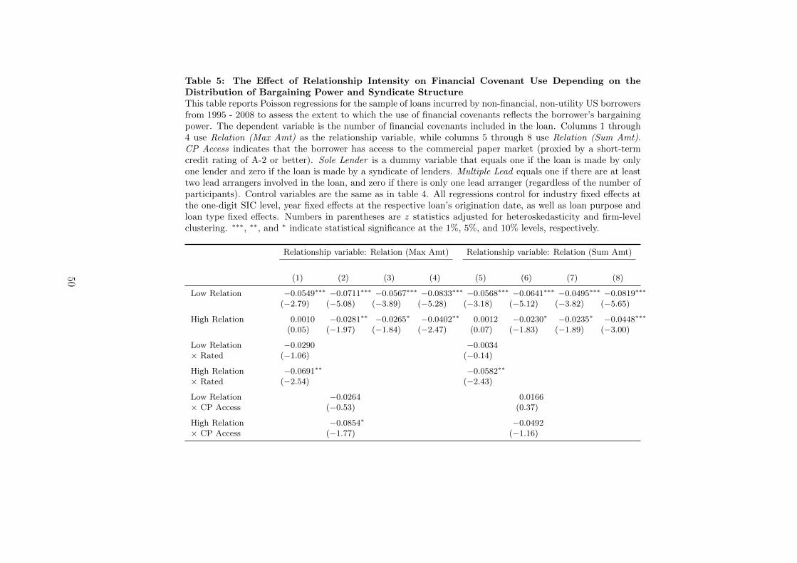
Table 5: The Effect of Relationship Intensity on Financial Covenant Use Depending on theDistribution of Bargaining Power and Syndicate StructureThis table reports Poisson regressions for the sample of loans incurred by non-financial, non-utility US borrowersfrom 1995 - 2008 to assess the extent to which the use of financial covenants reflects the borrower’s bargainingpower. The dependent variable is the number of financial covenants included in the loan. Columns 1 through4 use Relation (Max Amt) as the relationship variable, while columns 5 through 8 use Relation (Sum Amt).CP Access indicates that the borrower has access to the commercial paper market (proxied by a short-termcredit rating of A-2 or better). Sole Lender is a dummy variable that equals one if the loan is made by onlyone lender and zero if the loan is made by a syndicate of lenders. Multiple Lead equals one if there are at leasttwo lead arrangers involved in the loan, and zero if there is only one lead arranger (regardless of the number ofparticipants). Control variables are the same as in table 4. All regressions control for industry fixed effects atthe one-digit SIC level, year fixed effects at the respective loan’s origination date, as well as loan purpose andloan type fixed effects. Numbers in parentheses are z statistics adjusted for heteroskedasticity and firm-levelclustering. ∗∗∗, ∗∗, and ∗ indicate statistical significance at the 1%, 5%, and 10% levels, respectively.

Relationship variable: Relation (Max Amt) Relationship variable: Relation (Sum Amt)

(1) (2) (3) (4) (5) (6) (7) (8)

Low Relation −0.0549∗∗∗ −0.0711∗∗∗ −0.0567∗∗∗ −0.0833∗∗∗ −0.0568∗∗∗ −0.0641∗∗∗ −0.0495∗∗∗ −0.0819∗∗∗

(−2.79) (−5.08) (−3.89) (−5.28) (−3.18) (−5.12) (−3.82) (−5.65)

High Relation 0.0010 −0.0281∗∗ −0.0265∗ −0.0402∗∗ 0.0012 −0.0230∗ −0.0235∗ −0.0448∗∗∗

(0.05) (−1.97) (−1.84) (−2.47) (0.07) (−1.83) (−1.89) (−3.00)

Low Relation −0.0290 −0.0034× Rated (−1.06) (−0.14)

High Relation −0.0691∗∗ −0.0582∗∗

× Rated (−2.54) (−2.43)

Low Relation −0.0264 0.0166× CP Access (−0.53) (0.37)

High Relation −0.0854∗ −0.0492× CP Access (−1.77) (−1.16)

50

Table 5: The Effect of Relationship Intensity on Financial Covenant Use Depending on theDistribution of Bargaining Power and Syndicate Structure — Continued

Relationship variable: Relation (Max Amt) Relationship variable: Relation (Sum Amt)

(1) (2) (3) (4) (5) (6) (7) (8)

Low Relation −0.0718∗ −0.0873∗∗

× Sole Lender (−1.77) (−2.29)

High Relation −0.0368 −0.0507× Sole Lender (−0.84) (−1.21)

Low Relation 0.0433 0.0575∗∗

× Multiple Lead (1.41) (2.22)

High Relation 0.0262 0.0544∗∗

× Multiple Lead (0.92) (2.26)

CP Access −0.1380∗∗∗ −0.1772∗∗∗

(−2.89) (−4.32)

Sole Lender −0.0398 −0.0271(−0.97) (−0.70)

Multiple Lead −0.0376 −0.0532∗∗

(−1.41) (−2.49)

Control variables Yes Yes Yes Yes Yes Yes Yes Yes

Industry effects Yes Yes Yes Yes Yes Yes Yes Yes

Year effects Yes Yes Yes Yes Yes Yes Yes Yes

Loan purpose effects Yes Yes Yes Yes Yes Yes Yes Yes

Loan type effects Yes Yes Yes Yes Yes Yes Yes Yes

Observations 7923 7923 7923 7923 7923 7923 7923 7923

51

Table 6: The Effect of Relationship Intensity on Financial Covenant Use Dependingon the Borrower’s Information OpacityThis table reports Poisson regressions for the sample of loans incurred by non-financial, non-utility US borrowers from 1995 - 2008 to assess the extent to which the use of financial covenantsreflects the borrower’s information opacity. The dependent variable is the number of financialcovenants included in the loan. Relation (Max Amt) is used as the relationship variable, butresults using Relation (Sum Amt) are qualitatively and quantitatively similar. Small Borrower isa dummy variable indicating that the borrower’s size is below the median size of borrowers in thesame year. Hightech is a dummy variable that equals one if the borrower is a member of a hightechindustry as defined in Loughran and Ritter (2004). Low Analyst indicates that the number ofanalysts covering the borrower according to the I/B/E/S detail files is below the median numberof analysts for borrowers in that year. High Forecast Disp. equals one if the dispersion of analystforecasts for a firm’s earnings per share (EPS) is above the sample median in that year, andzero otherwise. Forecast dispersion for a firm is measured as the standard deviation of EPSforecasts divided by the absolute value of the mean EPS forecast in the I/B/E/S summary file.The dummy variable NASDAQ indicates that the firm’s stock traded on NASDAQ at the pointof contracting the loan, according to CRSP. Control variables are the same as in table 4. Allregressions control for industry fixed effects at the one-digit SIC level, year fixed effects at therespective loan’s origination date, as well as loan purpose and loan type fixed effects. Numbersin parentheses are z statistics adjusted for heteroskedasticity and firm-level clustering. ∗∗∗, ∗∗,and ∗ indicate statistical significance at the 1%, 5%, and 10% levels, respectively.

(1) (2) (3) (4) (5) (6)

Low Relation −0.0798∗∗∗ −0.0690∗∗∗ −0.0690∗∗∗ −0.0594∗∗∗ −0.0743∗∗∗ −0.0555∗∗∗

(−4.24) (−4.77) (−4.75) (−3.24) (−3.58) (−3.10)

High Relation −0.0643∗∗∗ −0.0260∗ −0.0306∗∗ −0.0613∗∗∗ −0.0631∗∗∗ −0.0473∗∗∗

(−3.59) (−1.74) (−2.07) (−3.50) (−3.17) (−2.67)

Low Relation 0.0228× Small Borrower (0.82)

High Relation 0.0660∗∗

× Small Borrower (2.44)

Low Relation −0.0261× S&P 500 (−0.63)

High Relation −0.0597× S&P 500 (−1.63)

Low Relation −0.0316× Hightech (−0.82)

High Relation −0.0162× Hightech (−0.40)

Low Relation −0.0089× Low Analyst (−0.33)

High Relation 0.0575∗∗

× Low Analyst (2.21)

Low Relation 0.0022× High Forecast Disp. (0.07)

High Relation 0.0268× High Forecast Disp. (0.98)

52

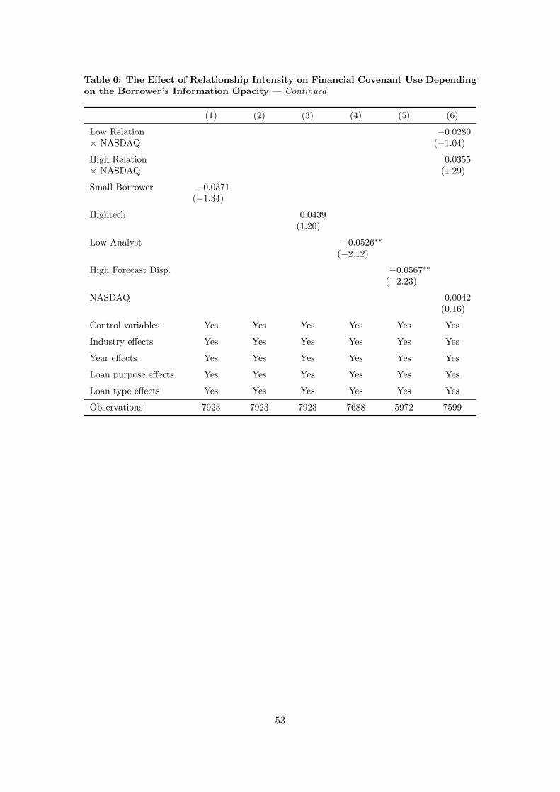
Table 6: The Effect of Relationship Intensity on Financial Covenant Use Dependingon the Borrower’s Information Opacity — Continued

(1) (2) (3) (4) (5) (6)

Low Relation −0.0280× NASDAQ (−1.04)

High Relation 0.0355× NASDAQ (1.29)

Small Borrower −0.0371(−1.34)

Hightech 0.0439(1.20)

Low Analyst −0.0526∗∗

(−2.12)

High Forecast Disp. −0.0567∗∗

(−2.23)

NASDAQ 0.0042(0.16)

Control variables Yes Yes Yes Yes Yes Yes

Industry effects Yes Yes Yes Yes Yes Yes

Year effects Yes Yes Yes Yes Yes Yes

Loan purpose effects Yes Yes Yes Yes Yes Yes

Loan type effects Yes Yes Yes Yes Yes Yes

Observations 7923 7923 7923 7688 5972 7599

53

Table 7: The Relationship Effect on Yield Spreads and Non-financial CovenantsThis table reports the effect of relationship intensity on the all-in spread drawn and non-financial covenants for the sample of loans incurredby non-financial, non-utility US borrowers from 1995 - 2008. Regressions (1) through (7) are ordinary least squares regressions where thedependent variable is the all-in yield spread over LIBOR that the borrower pays on each dollar drawn down on the loan. Regressions (8) and(9) are Poisson regressions where the dependent variable is the number of non-financial covenants attached to the loan. The regressions usethe Relation (Max Amt) measure described in table 3 as the measure of relationship intensity. Control variables are the same as in table 4.Variables used in the interaction terms are explained in tables 5 and 6. All regressions control for industry fixed effects at the one-digit SIClevel, year fixed effects at the respective loan’s origination date, as well as loan purpose and loan type fixed effects. Numbers in parenthesesare t-statistics (regressions (1) through (7)) and z statistics (regressions (8) and (9)) adjusted for heteroskedasticity and firm-level clustering.∗∗∗, ∗∗, and ∗ indicate statistical significance at the 1%, 5%, and 10% levels, respectively.

All-In Spread Drawn Non-financial Covenants

(1) (2) (3) (4) (5) (6) (7) (8) (9)

Relation −9.5481∗∗∗ −15.3146∗∗∗ −3.6334 −5.7208∗ 0.6450 −9.8641∗∗∗ −0.0547∗∗∗

(−3.64) (−4.22) (−1.06) (−1.82) (0.20) (−3.27) (−2.78)

Low Relation 1.7109 −0.0125(0.50) (−0.51)

High Relation −6.7575∗∗ −0.0590∗∗

(−2.06) (−2.37)

Relation 14.1106∗∗∗

× Rated (2.84)

Relation −10.2848∗∗

× Small Borrower (−2.06)

Relation −3.2219× NASDAQ (−0.62)

Relation −8.8281∗

× High Forecast Disp. (−1.70)

Relation 0.7034× Multiple Lead (0.12)

54

Table 7: The Relationship Effect on Yield Spreads and Non-financial Covenants — Continued

All-In Spread Drawn Non-financial Covenants

(1) (2) (3) (4) (5) (6) (7) (8) (9)

Small Borrower 22.5165∗∗∗

(4.32)

NASDAQ 11.4741∗∗

(2.43)

High Forecast Disp. 26.7162∗∗∗

(6.25)

Multiple Lead 7.0896(1.32)

Control variables Yes Yes Yes Yes Yes Yes Yes Yes Yes

Industry effects Yes Yes Yes Yes Yes Yes Yes Yes Yes

Year effects Yes Yes Yes Yes Yes Yes Yes Yes Yes

Loan purpose effects Yes Yes Yes Yes Yes Yes Yes Yes Yes

Loan type effects Yes Yes Yes Yes Yes Yes Yes Yes Yes

Observations 7649 7649 7649 7649 7371 5816 7649 7923 7923

55

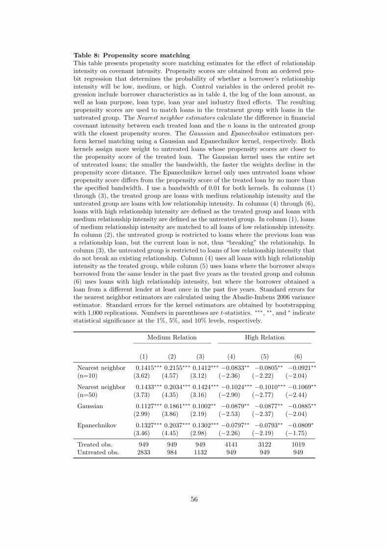
Table 8: Propensity score matchingThis table presents propensity score matching estimates for the effect of relationshipintensity on covenant intensity. Propensity scores are obtained from an ordered pro-bit regression that determines the probability of whether a borrower’s relationshipintensity will be low, medium, or high. Control variables in the ordered probit re-gression include borrower characteristics as in table 4, the log of the loan amount, aswell as loan purpose, loan type, loan year and industry fixed effects. The resultingpropensity scores are used to match loans in the treatment group with loans in theuntreated group. The Nearest neighbor estimators calculate the difference in financialcovenant intensity between each treated loan and the n loans in the untreated groupwith the closest propensity scores. The Gaussian and Epanechnikov estimators per-form kernel matching using a Gaussian and Epanechnikov kernel, respectively. Bothkernels assign more weight to untreated loans whose propensity scores are closer tothe propensity score of the treated loan. The Gaussian kernel uses the entire setof untreated loans; the smaller the bandwidth, the faster the weights decline in thepropensity score distance. The Epanechnikov kernel only uses untreated loans whosepropensity score differs from the propensity score of the treated loan by no more thanthe specified bandwidth. I use a bandwidth of 0.01 for both kernels. In columns (1)through (3), the treated group are loans with medium relationship intensity and theuntreated group are loans with low relationship intensity. In columns (4) through (6),loans with high relationship intensity are defined as the treated group and loans withmedium relationship intensity are defined as the untreated group. In column (1), loansof medium relationship intensity are matched to all loans of low relationship intensity.In column (2), the untreated group is restricted to loans where the previous loan wasa relationship loan, but the current loan is not, thus “breaking” the relationship. Incolumn (3), the untreated group is restricted to loans of low relationship intensity thatdo not break an existing relationship. Column (4) uses all loans with high relationshipintensity as the treated group, while column (5) uses loans where the borrower alwaysborrowed from the same lender in the past five years as the treated group and column(6) uses loans with high relationship intensity, but where the borrower obtained aloan from a different lender at least once in the past five years. Standard errors forthe nearest neighbor estimators are calculated using the Abadie-Imbens 2006 varianceestimator. Standard errors for the kernel estimators are obtained by bootstrappingwith 1,000 replications. Numbers in parentheses are t-statistics. ∗∗∗, ∗∗, and ∗ indicatestatistical significance at the 1%, 5%, and 10% levels, respectively.

Medium Relation High Relation

(1) (2) (3) (4) (5) (6)

Nearest neighbor 0.1415∗∗∗ 0.2155∗∗∗ 0.1412∗∗∗ −0.0833∗∗ −0.0805∗∗ −0.0921∗∗

(n=10) (3.62) (4.57) (3.12) (−2.36) (−2.22) (−2.04)

Nearest neighbor 0.1433∗∗∗ 0.2034∗∗∗ 0.1424∗∗∗ −0.1024∗∗∗ −0.1010∗∗∗ −0.1069∗∗

(n=50) (3.73) (4.35) (3.16) (−2.90) (−2.77) (−2.44)

Gaussian 0.1127∗∗∗ 0.1861∗∗∗ 0.1002∗∗ −0.0879∗∗ −0.0877∗∗ −0.0885∗∗

(2.99) (3.86) (2.19) (−2.53) (−2.37) (−2.04)

Epanechnikov 0.1327∗∗∗ 0.2037∗∗∗ 0.1302∗∗∗ −0.0797∗∗ −0.0793∗∗ −0.0809∗

(3.46) (4.45) (2.98) (−2.26) (−2.19) (−1.75)

Treated obs. 949 949 949 4141 3122 1019Untreated obs. 2833 984 1132 949 949 949

56

Table 9: Instrumental Variables EstimationThis table shows results for the relationship effects on financial covenant intensity from two-stageleast squares (2SLS) estimation. Three different models are presented that use different sets of in-struments. For each model, the column denoted 1st Stage shows the results of an ordered probitmodel, where the dependent variable equals one for low, two for medium, and three for high relation-ship intensity. Predicted probabilities for low and high relationship intensity from this model are usedas instruments in the first stage of the 2SLS estimation. The column denoted IV shows the 2SLSresult for financial covenant intensity. Relationship intensity is calculated using the Relation (MaxAmt) measure defined in table 3. The instruments include the log of one plus the distance betweenthe borrower’s headquarters and the headquarters of the closest lead arranger, a dummy variablethat indicates whether the borrower’s and the lead arranger’s headquarters are in the same state,the log of the total assets of the median firm in the borrower’s Fama-French 38 industry in the yearprior to entering the loan agreement, as well as the log of the age of the oldest firm in the borrower’sFama-French 38 industry. Firm age is calculated as 2008 minus the year of the initial public offeringas recorded in Compustat. Control variables are described in table 4. Cut 1 and Cut 2 refer to thecut points for the latent variable in the ordered probit model. All regressions control for industryfixed effects at the one-digit SIC level, year fixed effects at the respective loan’s origination date, aswell as loan purpose and loan type fixed effects. Numbers in parentheses are t statistics (z statisticsin the case of the ordered probit) adjusted for heteroskedasticity and firm-level clustering. ∗∗∗, ∗∗,and ∗ indicate statistical significance at the 1%, 5%, and 10% levels, respectively. The Cragg-DonaldF-statistic and the Kleibergen-Paap rk F-statistic are tests for instrument weakness, where the for-mer assumes homoskedastic i.i.d. errors, while the latter is robust to clustered standard errors. Thecritical value from Stock and Yogo (2005) is the value that the Cragg-Donald F-statistic needs toexceed to reject the hypothesis that a test for the joint significance of the endogenous regressors withnominal size 5% has a true size of more than 10%. The Anderson-Rubin F-statistic tests whether theendogenous regressors are jointly zero and is robust to instrument weakness.

Model 1 Model 2 Model 3

1st Stage IV 1st Stage IV 1st Stage IV

Low Relation −2.0129∗∗∗ −2.1060∗∗∗ −1.5934∗∗∗

(−2.87) (−3.36) (−3.06)

High Relation −1.5611∗∗ −1.6120∗∗ −1.0471∗∗

(−2.07) (−2.51) (−2.02)

Ln(1+Distance) −0.0330∗∗ −0.0659∗∗∗ −0.0326∗∗

(−2.20) (−6.15) (−2.18)

Same State 0.2028∗∗∗ 0.2041∗∗∗

(3.22) (3.24)

Ln(Industry Median Size) −0.0605∗∗ −0.0823∗∗∗

(−2.35) (−3.07)

Ln(Industry Age) −0.1790∗∗

(−2.52)

Ln(Loan Amount) 0.2260∗∗∗ −0.0559∗∗∗ 0.2210∗∗∗ −0.0584∗∗∗ 0.2243∗∗∗ −0.0537∗∗∗

(8.61) (−2.91) (8.43) (−2.86) (8.58) (−3.21)

Ln(Assets) 0.0016 −0.0262∗ 0.0044 −0.0259∗ 0.0086 −0.0256∗∗

(0.06) (−1.84) (0.16) (−1.76) (0.31) (−2.05)

Leverage 0.2241∗ −0.0197 0.2219∗ −0.0252 0.2199∗ −0.0048(1.79) (−0.25) (1.77) (−0.32) (1.76) (−0.07)

57

Tangibility 0.0136 −0.0822∗ 0.0444 −0.0829∗ 0.0288 −0.0783∗

(0.14) (−1.69) (0.46) (−1.67) (0.30) (−1.84)

Current Ratio −0.0153 0.0052 −0.0127 0.0048 −0.0148 0.0084(−1.00) (0.55) (−0.83) (0.52) (−0.96) (1.08)

Ln(1+Coverage Ratio) 0.0798∗∗∗ 0.0348∗∗ 0.0786∗∗∗ 0.0343∗∗ 0.0788∗∗∗ 0.0290∗∗

(3.35) (2.35) (3.29) (2.35) (3.30) (2.39)

Rating −0.0340∗∗∗ 0.0204∗∗∗ −0.0335∗∗∗ 0.0205∗∗∗ −0.0344∗∗∗ 0.0234∗∗∗

(−3.03) (2.58) (−2.98) (2.68) (−3.07) (3.66)

Not rated −0.4148∗∗∗ 0.3309∗∗∗ −0.4018∗∗∗ 0.3329∗∗∗ −0.4147∗∗∗ 0.3566∗∗∗

(−2.81) (3.78) (−2.72) (3.85) (−2.81) (4.87)

MTB −0.0012 −0.0179 −0.0050 −0.0180 −0.0053 −0.0175∗

(−0.05) (−1.56) (−0.22) (−1.52) (−0.24) (−1.79)

S&P 500 −0.1618∗∗ −0.2148∗∗∗ −0.1608∗∗ −0.2157∗∗∗ −0.1740∗∗ −0.1964∗∗∗

(−2.30) (−4.73) (−2.27) (−4.94) (−2.47) (−5.45)

Ln(Maturity) 0.0553∗∗ 0.0582∗∗ 0.0555∗∗

(2.24) (2.21) (2.58)

Ln(Lenders) 0.0118 0.0079 0.0049(0.53) (0.31) (0.26)

Constant 2.2062∗∗∗ 2.2716∗∗∗ 1.7901∗∗∗

(3.11) (3.60) (3.49)

Cut 1 0.6248 0.6302 0.4041(1.38) (1.33) (0.78)

Cut 2 0.9784∗∗ 0.9835∗∗ 0.7583(2.16) (2.07) (1.47)

Industry effects Yes Yes Yes Yes Yes Yes

Year effects Yes Yes Yes Yes Yes Yes

Loan purpose effects Yes Yes Yes Yes Yes Yes

Loan type effects Yes Yes Yes Yes Yes Yes

Observations 6643 6643 6643 6643 6643 6643

Weak ID testsCragg-Donald F-stat. 4.32 6.26 7.00Kleibergen-Paap rk F-stat. 4.45 6.71 7.26Stock-Yogo (2005) crit. 7.03 7.03 7.03

Weak ID robust inferenceAnderson-Rubin F-stat. 18.100 18.028 17.092Anderson-Rubin p-value 0.000 0.000 0.000

58

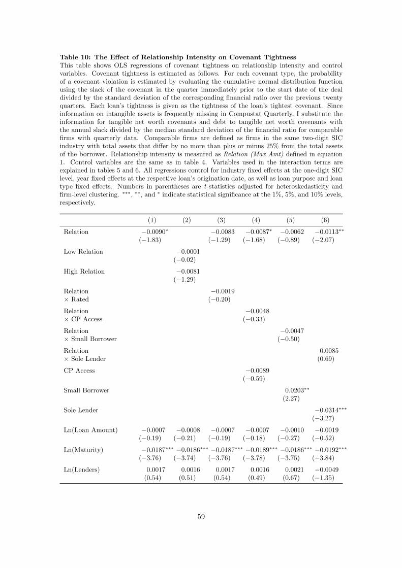
Table 10: The Effect of Relationship Intensity on Covenant TightnessThis table shows OLS regressions of covenant tightness on relationship intensity and controlvariables. Covenant tightness is estimated as follows. For each covenant type, the probabilityof a covenant violation is estimated by evaluating the cumulative normal distribution functionusing the slack of the covenant in the quarter immediately prior to the start date of the dealdivided by the standard deviation of the corresponding financial ratio over the previous twentyquarters. Each loan’s tightness is given as the tightness of the loan’s tightest covenant. Sinceinformation on intangible assets is frequently missing in Compustat Quarterly, I substitute theinformation for tangible net worth covenants and debt to tangible net worth covenants withthe annual slack divided by the median standard deviation of the financial ratio for comparablefirms with quarterly data. Comparable firms are defined as firms in the same two-digit SICindustry with total assets that differ by no more than plus or minus 25% from the total assetsof the borrower. Relationship intensity is measured as Relation (Max Amt) defined in equation1. Control variables are the same as in table 4. Variables used in the interaction terms areexplained in tables 5 and 6. All regressions control for industry fixed effects at the one-digit SIClevel, year fixed effects at the respective loan’s origination date, as well as loan purpose and loantype fixed effects. Numbers in parentheses are t-statistics adjusted for heteroskedasticity andfirm-level clustering. ∗∗∗, ∗∗, and ∗ indicate statistical significance at the 1%, 5%, and 10% levels,respectively.

(1) (2) (3) (4) (5) (6)

Relation −0.0090∗ −0.0083 −0.0087∗ −0.0062 −0.0113∗∗

(−1.83) (−1.29) (−1.68) (−0.89) (−2.07)

Low Relation −0.0001(−0.02)

High Relation −0.0081(−1.29)

Relation −0.0019× Rated (−0.20)

Relation −0.0048× CP Access (−0.33)

Relation −0.0047× Small Borrower (−0.50)

Relation 0.0085× Sole Lender (0.69)

CP Access −0.0089(−0.59)

Small Borrower 0.0203∗∗

(2.27)

Sole Lender −0.0314∗∗∗

(−3.27)

Ln(Loan Amount) −0.0007 −0.0008 −0.0007 −0.0007 −0.0010 −0.0019(−0.19) (−0.21) (−0.19) (−0.18) (−0.27) (−0.52)

Ln(Maturity) −0.0187∗∗∗ −0.0186∗∗∗ −0.0187∗∗∗ −0.0189∗∗∗ −0.0186∗∗∗ −0.0192∗∗∗

(−3.76) (−3.74) (−3.76) (−3.78) (−3.75) (−3.84)

Ln(Lenders) 0.0017 0.0016 0.0017 0.0016 0.0021 −0.0049(0.54) (0.51) (0.54) (0.49) (0.67) (−1.35)

59

Table 10: The Effect of Relationship Intensity on Covenant Tightness — Continued

(1) (2) (3) (4) (5) (6)

Ln(Assets) −0.0101∗∗∗ −0.0101∗∗∗ −0.0101∗∗∗ −0.0101∗∗∗ −0.0058 −0.0096∗∗∗

(−3.00) (−3.01) (−3.00) (−3.01) (−1.54) (−2.88)

Leverage 0.0617∗∗∗ 0.0616∗∗∗ 0.0617∗∗∗ 0.0623∗∗∗ 0.0606∗∗∗ 0.0605∗∗∗

(3.72) (3.71) (3.72) (3.75) (3.65) (3.65)

Tangibility −0.0626∗∗∗ −0.0625∗∗∗ −0.0626∗∗∗ −0.0624∗∗∗ −0.0626∗∗∗ −0.0635∗∗∗

(−5.55) (−5.55) (−5.55) (−5.54) (−5.57) (−5.64)

Current Ratio −0.0109∗∗∗ −0.0109∗∗∗ −0.0109∗∗∗ −0.0110∗∗∗ −0.0109∗∗∗ −0.0109∗∗∗

(−5.81) (−5.83) (−5.81) (−5.87) (−5.79) (−5.81)

Ln(1+Coverage Ratio) −0.0206∗∗∗ −0.0206∗∗∗ −0.0206∗∗∗ −0.0206∗∗∗ −0.0206∗∗∗ −0.0209∗∗∗

(−6.56) (−6.56) (−6.57) (−6.57) (−6.56) (−6.66)

Rating 0.0107∗∗∗ 0.0107∗∗∗ 0.0107∗∗∗ 0.0099∗∗∗ 0.0106∗∗∗ 0.0104∗∗∗

(7.63) (7.62) (7.58) (6.37) (7.52) (7.41)

Not rated 0.1433∗∗∗ 0.1432∗∗∗ 0.1418∗∗∗ 0.1337∗∗∗ 0.1392∗∗∗ 0.1384∗∗∗

(8.40) (8.40) (7.69) (7.03) (8.12) (8.11)

MTB −0.0016 −0.0016 −0.0016 −0.0016 −0.0014 −0.0014(−0.58) (−0.58) (−0.58) (−0.58) (−0.52) (−0.53)

S&P 500 −0.0095 −0.0096 −0.0095 −0.0064 −0.0119 −0.0079(−1.14) (−1.14) (−1.13) (−0.73) (−1.40) (−0.94)

Constant 0.1327∗∗ 0.1322∗∗ 0.1337∗∗ 0.1433∗∗∗ 0.1011∗ 0.1574∗∗∗

(2.43) (2.41) (2.43) (2.62) (1.83) (2.81)

Industry effects Yes Yes Yes Yes Yes Yes

Year effects Yes Yes Yes Yes Yes Yes

Loan purpose effects Yes Yes Yes Yes Yes Yes

Loan type effects Yes Yes Yes Yes Yes Yes

Observations 6947 6947 6947 6947 6947 6947Adj. R-squared 0.144 0.144 0.144 0.144 0.145 0.146

60

Table 11: Instrumental Variables Regressions for the Effect of Relationship Intensity on Covenant TightnessThis table shows 2SLS estimates of the effect of relationship intensity on covenant tightness. Relationship intensity is measured as Relation (MaxAmt) defined in equation 1. Columns (1) through (6) show results using the tightness measure as defined in table 10. Columns (7) through (10)measure tightness using only those covenants for which definitions across loans are relatively standardized (i.e. out of a random sample of twentycovenants, at least fifteen use the same definition (disregarding non-GAAP adjustments)): net worth, tangible net worth, EBITDA, debt to EBITDA,and liquidity covenants. For all other financial covenant types, less than ten contracts use the same definition. Column (1) uses the log of oneplus the distance between the borrower and the nearest lead arranger as the instrument. Column (2) shows the result when adding the three otherinstruments: a dummy variable that indicates whether the borrower’s and the lead arranger’s headquarters are in the same state, the log of the totalassets of the median firm in the borrower’s Fama-French 38 industry in the year prior to entering the loan agreement, as well as the log of the ageof the oldest firm in the borrower’s Fama-French 38 industry. The estimations in columns (3) through (10) again use the log of the borrower-lenderdistance as the instrument for relationship intensity. The interaction terms are instrumented by regressing relationship intensity on the log of theborrower-lender distance and the control variables, and interacting the predicted value for relationship intensity with the interaction variable. Theresulting variable is used as an instrument in the first stage of the 2SLS estimation, as discussed in Wooldridge (2002). Control variables are thesame as in table 4. Variables used in the interaction terms are explained in tables 5 and 6. All regressions control for industry fixed effects atthe one-digit SIC level, year fixed effects at the respective loan’s origination date, as well as loan purpose and loan type fixed effects. Numbers inparentheses are t-statistics adjusted for heteroskedasticity and firm-level clustering. ∗∗∗, ∗∗, and ∗ indicate statistical significance at the 1%, 5%,and 10% levels, respectively.

Tightness Tightness (Narrow Def.)

(1) (2) (3) (4) (5) (6) (7) (8) (9) (10)

Relation −0.1560∗∗ −0.0800 −0.1694∗∗ −0.1615∗∗ −0.1222 −0.2078∗∗∗ −0.2991∗∗∗ −0.2767∗∗∗ −0.2231∗∗ −0.3330∗∗∗

(−2.17) (−1.60) (−2.24) (−2.23) (−1.57) (−2.62) (−3.30) (−3.16) (−2.38) (−3.35)

Relation 0.0353 0.0949∗∗

× Rated (0.96) (2.15)

Relation 0.0957∗ 0.1774∗∗∗

× CP Access (1.73) (3.45)

Relation −0.0619 −0.0784∗

× Small Borrower (−1.64) (−1.77)

Relation 0.1506∗∗ 0.1725∗∗

× Sole Lender (2.28) (2.26)

CP Access −0.0850∗ −0.1450∗∗∗

(−1.91) (−3.60)

61

Table 11: Instrumental Variables Regressions for the Effect of Relationship Intensity on Covenant Tightness — Continued

Tightness Tightness (Narrow Def.)

(1) (2) (3) (4) (5) (6) (7) (8) (9) (10)

Small Borrower 0.0446∗ 0.0363(1.77) (1.17)

Sole Lender −0.1024∗∗∗ −0.1109∗∗∗

(−3.32) (−3.01)

Control variables Yes Yes Yes Yes Yes Yes Yes Yes Yes Yes

Industry effects Yes Yes Yes Yes Yes Yes Yes Yes Yes Yes

Year effects Yes Yes Yes Yes Yes Yes Yes Yes Yes Yes

Loan purpose effects Yes Yes Yes Yes Yes Yes Yes Yes Yes Yes

Loan type effects Yes Yes Yes Yes Yes Yes Yes Yes Yes Yes

Observations 5845 5845 5845 5845 5845 5845 4682 4682 4682 4682

Hansen’s J 2.76Hansen’s J p-value 0.431

Weak ID testsCragg-Donald F-stat. 37.30 17.24 18.66 18.60 18.65 17.71 15.03 14.80 14.86 13.94Kleibergen-Paap rk F-stat. 29.66 13.50 14.71 14.78 14.88 13.96 11.75 11.66 11.80 10.95Stock-Yogo (2005) crit. 16.38 24.58 7.03 7.03 7.03 7.03 7.03 7.03 7.03 7.03

62

Table 12: Reasons for exclusion of relationship sample loans from the final sampleFor all borrowers with at least one loan in the final sample, this table details why a loan that was used todetermine relationship intensity was not included in the final sample. Since data availability for financialcovenants requires the sample to start in 1995 and the relationship intensity measure uses a five-yearlookback period, loans made in 1990-1994 are used to determine relationship intensity, but are not usedin the final sample. For the same reason, loans where there was no previous loan during the past fiveyears are excluded from the final sample. Observations with a coverage ratio of less than minus one areexcluded from the final sample since the log of one plus the coverage ratio is one of the control variablesin the regressions. A few observations are excluded from the final sample because the firms are classifiedas financial, public administration or utility firms for these observations, even though they are classifiedas not belonging to these industries for other observations.

Number Percent

Covenant information missing 2316 29.36Loan prior to 1995 1815 23.01Company financials missing 1131 14.34Maturity missing 1086 13.77No loan in previous five years 1059 13.43No record in Compustat for fiscal year prior to loan start 169 2.14Coverage ratio less than minus one 147 1.86Link to Compustat unavailable for this package 63 0.80Foreign currency 41 0.52Firm classified as financial, public administration or utility during this year 39 0.49Syndication country foreign or unknown 18 0.23SIC code missing 4 0.05

Total 7888 100.00

63

Table 13: Heckman selection modelsThis table shows estimates of the effect of relationship intensity on financial covenant intensityusing OLS regressions and Heckman selection models. The dependent variable is the log of thefinancial covenant count. Columns 1 through 3 ask whether a selection effect is present in the loanswhere information on financial covenants is missing. Columns 4 through 6 assess selection effects inloans that are excluded from the final sample because they constitute a borrower’s first borrowing(during the previous five years) in DealScan. The total number of observations in columns 4and 5 does not match because some first borrowings also lack information on covenant intensity.Moving these observations to the analysis on missing covenant information yields qualitativelyand quantitatively similar results. Control variables are the same as in table 4. All regressionscontrol for industry fixed effects at the one-digit SIC level, year fixed effects at the respective loan’sorigination date, as well as loan purpose and loan type fixed effects. Numbers in parentheses are zstatistics adjusted for heteroskedasticity and firm-level clustering. ∗∗∗, ∗∗, and ∗ indicate statisticalsignificance at the 1%, 5%, and 10% levels, respectively.

Missing covenant information First borrowing

OLS Heckman model OLS Heckman modelOutcome Selection Outcome Selection

Low Relation −0.0822∗∗∗ −0.0822∗∗∗ −0.0818∗∗∗ −0.0631∗∗∗

(−5.32) (−5.34) (−5.29) (−4.66)

High Relation −0.0368∗∗ −0.0368∗∗ −0.0359∗∗ −0.0274∗∗

(−2.35) (−2.36) (−2.29) (−1.99)

First Borrowing −0.0421∗∗

(−2.08)

Ln(Loan Amount) −0.0238∗∗ −0.0236∗∗ −0.0897∗∗∗ −0.0193∗∗ −0.0194∗ 0.0092(−2.49) (−2.46) (−3.06) (−2.12) (−1.90) (0.32)

Ln(Maturity) 0.0127 0.0124 0.0383 0.0127 0.0244∗ −0.0890∗∗

(0.97) (0.96) (1.03) (1.05) (1.79) (−2.38)

Ln(Lenders) 0.0557∗∗∗ 0.0544∗∗∗ 0.4180∗∗∗ 0.0521∗∗∗ 0.0245∗∗∗ 0.0845∗∗∗

(6.88) (6.46) (17.04) (6.68) (2.84) (3.20)

Ln(Assets) −0.0230∗∗∗ −0.0223∗∗∗ −0.2071∗∗∗ −0.0236∗∗∗ −0.0338∗∗∗ 0.0728∗∗∗

(−2.69) (−2.61) (−7.42) (−2.85) (−3.73) (2.91)

Leverage 0.0633 0.0642 −0.3015∗∗ 0.0465 0.0475 0.0451(1.59) (1.63) (−2.44) (1.22) (1.17) (0.39)

Tangibility −0.0605∗∗ −0.0606∗∗ 0.0183 −0.0549∗ −0.0613∗∗ −0.0074(−2.02) (−2.04) (0.20) (−1.94) (−2.04) (−0.10)

Current Ratio 0.0107∗∗ 0.0106∗∗ 0.0382∗∗ 0.0097∗∗ 0.0101∗ −0.0038(2.18) (2.16) (2.16) (2.10) (1.93) (−0.26)

Ln(1+Coverage Ratio) 0.0358∗∗∗ 0.0357∗∗∗ 0.0408 0.0345∗∗∗ 0.0372∗∗∗ −0.0840∗∗∗

(4.75) (4.75) (1.63) (4.90) (4.78) (−3.93)

Rating 0.0272∗∗∗ 0.0271∗∗∗ 0.0121 0.0283∗∗∗ 0.0259∗∗∗ 0.0201(6.63) (6.65) (1.11) (6.92) (6.14) (1.32)

Not rated 0.3756∗∗∗ 0.3752∗∗∗ 0.1319 0.3863∗∗∗ 0.3668∗∗∗ 0.1842(7.18) (7.21) (0.93) (7.47) (6.82) (0.96)

MTB −0.0102 −0.0101 −0.0220 −0.0108∗ −0.0076 −0.0206(−1.60) (−1.59) (−0.92) (−1.78) (−1.12) (−1.11)

64

Table 13: Heckman selection models — Continued

Missing covenant information First borrowing

OLS Heckman model OLS Heckman modelOutcome Selection Outcome Selection

S&P 500 −0.1725∗∗∗ −0.1727∗∗∗ 0.0498 −0.1698∗∗∗ −0.1504∗∗∗ −0.0891(−7.25) (−7.29) (0.75) (−7.34) (−6.21) (−1.12)

Constant 0.6180∗∗∗ 0.6239∗∗∗ 0.3962 0.6320∗∗∗ 0.8542∗∗∗ 0.3659(5.51) (5.55) (1.09) (5.83) (7.08) (1.02)

Industry effects Yes Yes Yes Yes Yes Yes

Year effects Yes Yes Yes Yes Yes Yes

Loan purpose effects Yes Yes Yes Yes Yes Yes

Loan type effects Yes Yes Yes Yes Yes Yes

Observations 7923 10237 8708 8982Censored Observations 2314 1059Rho −0.024 −0.955χ2 0.18 1023.51p-value 0.67 0.00

65

Table A-1: Covenant intensity and tightness as predictors ofcovenant violationsThis table shows marginal effects from Probit regressions predicting whethera new covenant violation occurs during the time a loan is active. Quarterlycovenant violation data are from Nini et al. (2010). As suggested in theirpaper, covenant violations are judged as new if the firm has not reported aviolation in the previous four quarters. Ln(FinCov) is the log of the numberof financial covenants attached to the loan (covenant intensity). Covenanttightness is defined as in table 10. Control variables are the same as in table4. All regressions control for industry fixed effects at the one-digit SIC level,year fixed effects at the respective loan’s origination date, as well as loanpurpose and loan type fixed effects. Numbers in parentheses are z statisticsadjusted for heteroskedasticity and firm-level clustering. ∗∗∗, ∗∗, and ∗ indicatestatistical significance at the 1%, 5%, and 10% levels, respectively.

(1) (2) (3)

Ln(FinCov) 0.0598∗∗∗ 0.0588∗∗∗

(4.20) (3.58)

Tightness 0.1869∗∗∗ 0.1665∗∗∗

(5.28) (4.65)

Ln(Loan Amount) −0.0174∗ −0.0183∗ −0.0178∗

(−1.87) (−1.84) (−1.78)

Ln(Maturity) 0.1153∗∗∗ 0.1177∗∗∗ 0.1164∗∗∗

(8.17) (7.88) (7.82)

Ln(Lenders) 0.0029 0.0089 0.0064(0.34) (0.97) (0.70)

Ln(Assets) −0.0253∗∗∗ −0.0255∗∗∗ −0.0240∗∗

(−2.85) (−2.67) (−2.50)

Leverage −0.0111 −0.0293 −0.0318(−0.27) (−0.68) (−0.74)

Tangibility −0.0015 −0.0041 −0.0008(−0.04) (−0.12) (−0.02)

Current Ratio 0.0085 0.0116∗∗ 0.0108∗

(1.53) (1.99) (1.85)

Ln(1+Coverage Ratio) −0.0130∗ −0.0082 −0.0095(−1.69) (−0.98) (−1.14)

Rating 0.0166∗∗∗ 0.0156∗∗∗ 0.0142∗∗∗

(3.89) (3.40) (3.05)

Not rated 0.2300∗∗∗ 0.2130∗∗∗ 0.1951∗∗∗

(4.12) (3.58) (3.22)

MTB −0.0247∗∗∗ −0.0264∗∗∗ −0.0260∗∗∗

(−3.16) (−3.24) (−3.19)

S&P 500 0.0438 0.0310 0.0412(1.51) (1.01) (1.34)

Industry effects Yes Yes Yes

Year effects Yes Yes Yes

Loan purpose effects Yes Yes Yes

Loan type effects Yes Yes Yes

Observations 7354 6490 6490

66