Why did bank stocks crash during COVID-19?

1

Why did bank stocks crash during COVID-19?

Viral V. Acharya† Robert Engle‡ Sascha Steffen*

March 8, 2021

Abstract

We study the crash of bank stock prices during the COVID-19 pandemic. We find evidence

consistent with a “credit line drawdown channel”. Stock prices of banks with large ex-ante exposures to undrawn credit lines as well as large ex-post gross drawdowns decline more. The

effect is attenuated for banks with higher capital buffers. These banks reduce term loan lending, even after policy measures were implemented. We conclude that bank provision of credit lines

appears akin to writing deep out-of-the-money put options on aggregate risk; we show how the resulting contingent leverage and stock return exposure can be incorporated tractably into bank

capital stress tests.

Keywords: Credit lines, liquidity risk, bank capital, loan supply, stress tests, pandemic,

COVID-19 JEL-Classification: G01, G21.

We thank Jennie Bai, Tobias Berg, Allen Berger, Christa Bouwman, Olivier Darmouni, Darrel Duffie, Max Jager, Rafael Repullo, Phil Strahan, Daniel Streitz, Anjan Thakor, Josef Zechner and participants at the 2020 Federal Reserve Stress Testing Conference and seminar participants at the Annual Columbia SIPA/BPI Bank Regulation Research Conference, Banco de Portugal, Bank of England, CAF, Federal Reserve Bank of Cleveland, NYU Stern Finance, RIDGE Workshop on Financial Stability, University of Southern Denmark, University of Durham, Villanova Webinars in Financial Intermediation, the Volatility and Risk Institute, World Bank, WU Vienna, for comments and suggestions and Sophie-Dorothee Rothermund and Christian Schmidt for excellent research assistance. Robert Engle would like to thank NSF 2018923, Norges Bank project “Financial Approach to Climate Risk” and Interamerican Development Bank Contract #C- RG-T3555-P001 for research support to the Volatility and Risk Institute of NYU Stern. †NYU Stern School of Business, 44 West Fourth Street, Suite 9-65, New York, NY 10012-1126, Email: [email protected], Tel: +1 212 998 0354. ‡NYU Stern School of Business, 44 West Fourth Street, Suite 9-62, New York, NY 10012-1126, Email: [email protected], Tel: +1 212 998 0710. *Frankfurt School of Finance & Management, Adickesallee 32-34, 60323 Frankfurt, Germany, Email: [email protected], Tel: +49 (0)69 154008-794.

2

1. Introduction

This paper investigates the crash of bank stocks during the COVID-19 pandemic and studies

its causes, consequences and policy implications.

The pandemic and subsequent government-imposed lockdowns put the liquidity-

insurance function of banks for the U.S. economy to a real-life test, as firms’ cash flows dropped

as much as 100%, while operating and financial leverage remained sticky. As a consequence,

U.S. firms with pre-arranged credit lines from banks drew down their undrawn facilities at a far

greater intensity than in past recessions. Panel A of Figure 1 shows a sharp acceleration of

credit-line drawdowns of publicly listed U.S. firms since March 1, 2020.1 Within three weeks,

public firms drew down more than USD 300bn, with drawdowns particularly concentrated

among riskier BBB-rated and non-investment-grade firms.2 Recent data shows that firms

benefited from having access to credit lines during the pandemic when capital market funding

froze (e.g., Acharya and Steffen, 2020a; Chodorow-Reich et al., 2020; Greenwald et al., 2020).

Banks, however, faced unprecedented aggregate demand for credit-line drawdowns when the

pandemic broke out at the beginning of March 2020. Since then, banks’ share prices have

persistently underperformed those of non-financial firms (Panel B of Figure 1).3

[Figure 1 about here]

We construct a new measure of the balance-sheet liquidity risk of banks defined as

undrawn commitments plus wholesale finance minus cash or cash equivalents (all relative to

1 Ford Motor Company was one of the largest U.S. firms to draw down its credit lines in March 2020, withdrawing USD 15.4bn (Appendix I shows the SEC filings). It was still BBB- rated by S&P at this time. With USD 20bn in cash, credit lines make up a large part of its overall liquidity. Based on its loan contracts, Ford pays 15bps in commitment fees for any dollar-undrawn credit and 125bps once credit lines have been drawn down. Ford thus paid USD 23.1mn as long as the credit line was undrawn, and USD 192.5mn annually once the credit line was fully utilized. Importantly, once Ford was downgraded to non-investment grade, commitment fees increased to 25bps and credit spreads to 175bps, an increase of 67% and 40%, respectively. 2 Li et al. (2020) show – using call report data – that drawdowns amounted to more than USD 500bn, likely because of private firms, even further increasing the pressure on bank balance sheets. 3 Bank stock prices hardly recovered even after the monetary and fiscal measures (i.e., after 3/23/2020) until the end of Q2 2020. However, average stock returns increased about 17% during this period (relative to a mean decline of 65% in the month before).

3

assets).4 We show that our measure of the liquidity risk of banks is important to understand the

decline of bank stock prices during the first phase of the pandemic, i.e. from 1/1/2020 until

3/23/2020, before decisive monetary and fiscal support measures were introduced. During this

phase of the pandemic, stock prices of banks with high balance-sheet liquidity risk

underperformed relative to those of banks with low balance-sheet liquidity risk, controlling for

market beta and key bank performance measures (capitalization, asset quality, profitability,

liquidity and investments).5 A one-standard-deviation increase in liquidity risk decreased stock

returns by about 5% during this period, or 7.4% of the unconditional mean return.

We also posit alternative explanations for the underperformance of bank stock prices

such as real estate exposure, warehousing activities of dealer-banks, or the presence of large

derivative portfolios. Several other bank exposures came under stress during the pandemic (e.g.,

to the retail, hotel and leisure sectors). Exposure to oil prices also emerged as an important risk

that might have contributed to the crash of bank stocks.6 Moreover, bank exposures to retail

credit line commitments and consumer loans were also at risk of losses when unemployment

rates and furloughs rose. Using bank-loan-level exposure data to these sectors sourced from the

Dealscan database, we show that these risk factors do significantly affect bank stock returns.

These exposures, however, appear to be orthogonal to balance-sheet liquidity risk. Furthermore,

4 We develop and use a comprehensive measure of liquidity risk because the relative importance of its components (unused C&I commitments or wholesale funding) might change over time. For example, bank reliance on wholesale funding has continued to decline since the global financial crisis while unused C&I loans have increased over 2017-2019. 5 In contrast to bank capital, there is no consensus in the literature on how to measure liquidity, and those measures that have been used follow different concepts. For example, Deep and Schaefer (2004) use the difference between scaled liquid assets and liabilities, focusing on on-balance-sheet components of liquidity. Berger and Bouwman (2009) construct a comprehensive liquidity measure using on- and off-balance-sheet components. Both measures follow the concept of liquidity creation. Our measure focuses on liquidity risk, particularly during aggregate economic downturns, through credit lines and short-term wholesale funding. Bai et al. (2018) use on- and off-balance-sheet items to construct a measure of liquidity risk incorporating current market liquidity conditions. While their measure is more complex and reacts (contemporaneously) once market liquidity conditions deteriorate, our measure is a relatively simple (ex-ante) measure of bank exposure to liquidity risk. We compare our measure to both previous measures, highlighting similarities and differences in section 8 of this paper. 6 The energy sector was severely hit when on March 9, 2020 oil prices dropped by more than 20% on a single day. Both Saudi Arabia and Russia, two of the world’s largest oil producers, decided to increase their oil output considerably having failed to reach an agreement with OPEC on possible production cuts. After this oil price shock, oil price volatility increased by more than six times (to more than 100% on an annualized basis) and energy stocks crashed. Banks are heavily exposed through loans provided to this sector.

4

when we include measures of a bank’s capital shortfall conditional on a severe market

correction (for example, SRISK7, which relies in turn on LRMES, a measure of stock returns

conditional on market downturns), but do not take into account the role of undrawn credit lines,

the explanatory power for bank stock returns remains unaffected.

To summarize, while other factors are important in understanding the performance of

bank stock prices at the beginning of the pandemic, the aggregate drawdown risk associated

with bank credit lines does not appear to be captured in traditional measures of bank exposure

or systemic risk. That is, a bank’s “contingent leverage” associated with aggregate drawdowns

is akin to a deep out-of-the-money put option that is neither captured by a bank’s stock beta nor

by its (long-run) marginal expected shortfall (MES), or is possibly captured only ex-post, i.e.

with a lag, as the event causing aggregate drawdowns unfolds.

We then show that this cross-sectional explanatory power of balance-sheet liquidity risk

for bank stock returns is episodic in nature. Using separate cross-sectional regressions during

the months of January 2020, February 2020 and during the 3/1/2020 to 3/23/2020 period, we

show that liquidity risk explains stock returns only during the last period, when firms’ liquidity

demand through credit line drawdowns becomes highly correlated, but not before. We then

employ time-series tests for bank stock returns to shed further light on this result. Interacting

our bank-level liquidity risk measure with the aggregate measure of realized cumulative credit

line drawdowns, we show that (daily) bank stock returns are significantly lower when aggregate

drawdowns in the economy increase and banks have more balance-sheet liquidity risk. Further,

stock returns for banks with greater liquidity risk are lower, particularly when drawdowns of

riskier firms accelerate. Finally, these effects reverse only after monetary policy and fiscal

policy measures. There is a reversal of undrawn C&I credit lines on banks’ balance sheets in

Q2 and Q3 2020, but not to pre-COVID-19 levels. Consistently, we find that the episodic

7 See NYU Stern Volatility & Risk Institute, https://vlab.stern.nyu.edu/welcome/srisk, Acharya et al. (2016) and Brownlees and Engle (2017) for definition and estimation of LRMES and SRISK.

5

explanatory power of balance-sheet liquidity risk for bank stock returns also reverses following

policy measures.8

We confirm that the episodic co-movement of stock returns and the balance-sheet

liquidity risk of banks is not specific to aggregate drawdown risk during the pandemic, but was

also a feature of the global financial crisis (GFC) during 2007 to 2009. We use the same cross-

sectional tests as before and run them quarterly over the Q1 2007 to Q1 2009 period. We show

that liquidity risk for banks ignited in Q3 2007, i.e., in the first phase of the GFC when the

Asset Backed Commercial Paper (ABCP) market froze, as documented in Acharya et al.

(2013). Liquidity risk remained priced in the cross-section of bank stock returns (even increased

in economic magnitude) until the end of Q2 2008. The Federal Reserve and the U.S.

government responded to the economic fallout of the Lehman Brothers default with a variety

of measures to support the banking sector, following which we do not see any effect of liquidity

risk on bank stock returns. Acharya and Mora (2015) show that banks had deposit shortfalls

relative to credit line drawdowns during the GFC, unlike during the pandemic. In other words,

the episodic nature of liquidity risk contributing to bank stock returns during the pandemic finds

similar undertones during the GFC; the former caused by aggregate drawdown risk (credit lines)

and the latter by aggregate rollover risk (wholesale finance). Our liquidity risk measure for

banks spans both of these risks.

Next, we examine the reasons why bank stock prices were particularly sensitive to

undrawn C&I credit lines when the pandemic broke out. Does funding liquidity to source new

loans become a binding constraint for banks as deposit funding does not keep pace with credit

line drawdowns (the “funding channel”)? Or, does the drawdown of credit lines lock up bank

capital against term loans and impair bank loan origination, preventing banks from making

8 Interestingly, the Fed already conducted large interventions in the repo market on 3/12/2020. The OIS-spread, a measure for liquidity conditions in financial markets, reverted already following these interventions. They were, however, insufficient to stop the further decline of bank stock prices suggesting that liquidity was not the binding constraint for banks at the beginning of the COVID-19 pandemic.

6

possibly more profitable loans (the “capital channel”)?9 To distinguish between these channels,

we construct two proxies: (1) Gross drawdowns as the percentage change in credit line

drawdowns; and (2) Net drawdowns as the percentage change in drawdowns minus the change

in deposit funding. Holding gross drawdowns fixed, our measure of net drawdowns helps us

understand the importance of changes in bank deposits for bank stock returns. We find that

while bank stock returns during 1/1/2020 to 3/23/2020 are particularly sensitive to gross

drawdowns, they do not load significantly on net drawdowns. Importantly, a higher level of

bank capital buffer attenuates the negative effect of gross drawdowns on stock returns. These

results suggest that at the onset of the pandemic bank capital and not bank liquidity appears to

have been perceived as the binding constraint causing liquidity risk to adversely affect bank

stock returns. In this regard, the pandemic fallout for banks differs from that during the GFC

when banks struggled on the liquidity front to meet drawdowns (Acharya and Mora, 2015).

The development of credits spreads at the beginning of the pandemic suggests that this

phenomenon might have also affected loan market originations. We plot the time-series of

credit spreads in the loan and bond market over the Q1 2019 to Q3 2020 period in Figure 2. In

particular, we plot the loan-bond differential (Panel A of Figure 2) and find that that difference

between loan and bond spreads increased from about 2.5% to 3.5% following the outbreak of

COVID-19 and remained highly elevated, particularly driven by loans to riskier firms (Panel B

of Figure 2). Bond spreads, however, reverted back almost to pre-COVID levels (not shown).

This is consistent with the interpretation that bank health was materially affected by the

9 For the banks that provided credit lines to Ford Motors (as described in our introductory example in footnote 1 above), these commitments were (in aggregate) a USD 15.4bn off-balance-sheet C&I loan commitment as of 12/31/2019. The capital treatment of their commitment depends on whether banks follow the standardized (SA) or internal ratings-based (IRB) approach for credit risk. Under Basel III, the standardized approach differentiates between irrevocable and revocable commitments. Revocable commitments carry a credit conversion factor (CCF) of 10% and irrevocable commitments (with a maturity of more than 12 months) a CCF of 50%. Assuming an 8% capital requirement, an undrawn credit line thus requires funding in the range of 0.8% to 4% for banks using the SA. For IRB banks – as applies to most of our sample banks – the CCF might be considerably lower (Behn et al., 2016). In other words, a bank might need to fund 90% or more of the required capital when a credit line is drawn down and becomes a balance-sheet loan, which adversely impacts other business activities, particularly in an aggregate downturn.

7

pandemic, and not just temporarily, impacting the access of firms to bank loans as well as the

cost of bank credit.10

[Figure 2]

Investigating new loan originations, we find that banks with large credit-line drawdowns indeed

significantly reduced their supply of newly issued loans.11 We use a Khwaja and Mian (2008)

estimator and aggregate our data at a borrower x bank x loan type x month level, collapse the

sample into a pre- and post-COVID-19 period (where “post” is the period after 4/1/2020), and

saturate the estimation with borrower x bank x loan type fixed effects. We show that both the

number of loans as well as loan amounts are lower for banks with both higher gross and net

drawdowns after the breakout of the COVID-19 pandemic. Importantly, when we estimate

separately the effect on term loans and credit lines (using borrower x bank fixed effects), term

loan originations are substantially lower for banks with higher gross drawdowns, whereas new

credit line commitments decrease mainly for banks with higher net drawdowns. This confirms

that gross drawdowns reduce the capital available to banks and thus term lending, whereas

banks experiencing net drawdowns are reluctant to take on additional liquidity risk, but they

can issue term loans as long as they have capital to provide for them. Overall, there appear to

be long-term real consequences because of banks’ contingent leverage materializing from a

drawdown of credit lines during an aggregate shock.

A final key question is how can policy makers address aggregate drawdown risk in an

ex-ante manner? One possible way is for regulators to add the effect of drawdowns to stress

tests and require banks to fund these exposures with equity.12 In our last step, we therefore

10 The Senior Loan Officer Survey of the Federal Reserve also shows that at the end of Q3 2020, about 75% of loan officer reported a tightening of bank lending standards for small and medium/large firms. 11 The theoretical literature argues that a key function of bank capital is to absorb risk, i.e., more capital facilitates bank lending. Bhattacharya and Thakor (1993), Repullo (2004), von Thadden (2004), and Coval and Thakor (2005), among others, argue that capital increases risk-bearing capacity. Allen and Santomero (1998) and Allen and Gale (2004) show that banks with less capital might have to dispose of illiquid assets when facing an adverse shock. 12 We find that banks do not account for aggregate drawdown risk in fees or spreads when initiating new loan contracts. Moreover, drawdowns do also not appear to be constrained through covenants. We investigate all loan amendments during the post-COVID period and find that not a single loan amendment was initiated through a

8

quantify the capital shortfall that arises due to banks’ balance-sheet liquidity risk and show how

it can be incorporated tractably into bank stress tests. Acharya et al. (2012), Acharya et al.

(2016) and Brownlees and Engle (2017) developed the concept of SRISK, a measure of the

capital shortfall of a stressed aggregate market correction (e.g., 40% decline in the S&P 500

index), measured relative to an 8% requirement in terms of market value of equity to debt plus

market value of equity. This measure, however, does not account for the impact of credit lines,

which are off-balance-sheet or contingent liabilities. Given our results, such an impact can be

broken down into two components. First, contingent liabilities enter banks’ balance sheets as

realized liabilities during periods of stress. Using drawdown data during the COVID crisis, the

GFC and the 2000-2003 recession, we extrapolate the expected drawdown in a stress scenario

with a 40% market correction based on each of these three stressed periods. We find the

expected (incremental) drawdown rates in such a stress scenario to be in the range 11% to 23%.

Using these expected drawdown rates, we calculate the additional equity capital that would be

required to maintain adequacy against higher realized liabilities in periods of stress. Second,

we have to account for the negative episodic effect of liquidity risk on bank stock prices during

periods of stress. Using the loadings from our cross-sectional regressions of bank stock returns

on balance-sheet liquidity risk during the COVID-19 crisis, we estimate the additional equity

shortfall of banks based on their end of Q4 2019 market values of equity.

Summing both components, we show that the additional capital shortfall for the U.S.

banking sector as a whole due to balance-sheet liquidity risk amounted to more than USD 270bn

as of 12/31/2019 in a stress scenario of a 40% correction to the global stock market with the

top 10 banks contributing about USD 230bn. The incremental capital shortfall of the top 10

banks is about 1.5 times larger than the capital shortfall estimate without accounting for

contingent liabilities.

covenant violation. On the contrary, banks and firms regularly negotiated a covenant relief period early in the pandemic. In other words, contractual mechanisms also did not attenuate aggregate drawdowns at the start of the pandemic.

9

The paper proceeds as follows. We first describe the related literature. In Section 3, we

present the data. In Section 4, we describe our measure of balance-sheet liquidity risk and

investigate the effect of liquidity risk on bank stock returns. We investigate the liquidity

measure’s components in Section 5. Section 6 analyzes the funding vis-à-vis the capital channel

and also studies the consequences for the real economy. Section 7 illustrates how to incorporate

episodic liquidity risk of bank balance sheets in stress tests and assess capital shortfalls. We

provide a discussion of our results in section 8. Section 9 concludes.

2. Related literature

Our paper relates to the literature highlighting the role of banks as liquidity providers. Kashyap

et al. (2002) proposed a risk-management motive to understand the unique role of banks as

liquidity providers to both households and firms. As long as demand for deposits and loans is

not too highly correlated, banks can pool both types of customers and hold less (costly) liquid

assets. Gatev and Strahan (2006) build this idea and argue that banks can insure firms even

against systematic declines in liquidity because of deposit inflows during crises. Ivashina and

Scharfstein (2010) provide evidence of an acceleration of credit-line drawdowns during the

2007-2009 crisis as well as an increase in deposits. Acharya and Mora (2015) show that during

the 2007-2009 crisis – in which the banking system itself was at the center of the crisis – banks

faced a crisis as liquidity providers and could only perform this role because of significant

support from the government. Li et al. (2020) show that during the COVID-19 crisis, aggregate

deposit inflows were sufficient to fund the increase in liquidity demand. Acharya and Steffen

(2020b) use simulations based on drawdown scenarios from prior crises and arrive at similar

conclusions. Kapan and Minoiu (2020) show that banks exposed to larger credit-line

drawdowns reduce lending. None of these papers, however, explores the implications of banks

as liquidity providers for bank stock returns when drawdowns affect bank capital availability

for other intermediation functions, and especially when the realized risk is aggregate in nature.

10

There is a growing literature on the implications of COVID-19 for corporate finance,

and the use of credit lines in particular. Chodorow-Reich et al. (2020) show that drawdowns of

credit lines came exclusively from large firms during the first phase of the pandemic and

document that banks did not honor commitments to smaller firms. Greenwald et al. (2020) also

show that particularly large firms used their credit lines and banks with larger drawdowns

reduced term lending to small firms more relative to other banks. Darmouni and Siani (2020)

show that a large percentage of credit lines were repaid through bond issuances in Q2 and Q3

2020. By examining both gross drawdowns and net (of deposit inflows) drawdowns, we

demonstrate that credit-line drawdowns reduce banks’ franchise value because of binding

capital constraints. While banks with higher gross drawdowns reduce term lending, banks with

higher net drawdowns reduce credit line originations.13

Other papers consider stock price reactions to the COVID-19 pandemic, emphasizing

the importance of financial policies (Ramelli and Wagner forthcoming), financial constraints

and the cash needs of affected firms (Fahlenbrach, Rageth, and Stulz 2020), changing discount

rates because of higher uncertainty (Gormsen and Koijen 2020, Landier and Thesmar 2020),

and social-distancing measures (Pagano, Wagner and Zechner 2020). These papers focus on

stock prices of non-financial firms, not banks. Demirguc-Kunt et al. (2020) investigate the bank

stock market response to the COVID-19 pandemic and policy responses globally. They

highlight that the effectiveness of policy measures was dependent on bank capitalization and

fiscal space in the respective country. We focus instead on the implications of credit line

drawdowns for bank stock returns and the consequences for bank lending.

13 Other papers explore the determinants of credit-line drawdowns in previous crises. Ivashina and Scharfstein (2010) document an acceleration of credit line drawdowns during the 2007-2009 crisis; their evidence is consistent with ours. Berg et al. (2016) show that credit lines are more likely to be used if a borrower’s economic performance deteriorates, particularly for non-IG and unrated firms. Berg et al. (2017) show that U.S. firms’ drawdown behavior is particularly sensitive to the overall market return. We show that pandemic drawdowns have been more intense but similar in spirit.

11

Our paper also contributes methodologically to the literature on bank stress tests. After

the 2007-2009 crisis, a variety of measures were developed to quantify the systemic risk of the

banking sector. In addition to the SRISK measure of Acharya et al. (2012), Acharya et al.

(2016) and Brownlees and Engle (2017), which we discussed in the introduction, Adrian and

Brunnermeier (2015) develop the concept “CoVaR”, which measures the risk to the financial

system conditional on a bank being in distress. These measures, however, do not look at the

role of contingent liabilities of banks or their episodic impact on bank returns; we show how

these important considerations can be embedded into bank stress tests.

3. Data

We collect data for all publicly listed bank-holding companies of commercial banks in the U.S.

To construct or main dataset, we follow Acharya and Mora (2015) and drop all banks with total

assets below USD 100mn at the end of 2019 and also only keep those banks that we can match

to the CRSP/Compustat database. All financial variables (on the holding-company level) are

obtained from the call reports (FR-Y9C) and augmented with data sourced from SNL Financial.

We keep only those banks for which we have all data available for our main specifications

during the COVID-19 pandemic, which limits our sample to 127 U.S. bank-holding companies

(accounting for about 80% of all outstanding credit lines).14 All variables are explained below

or in Appendix II.

We obtain daily stock returns for our sample banks from CRSP. We manually match

these banks to the Thomson Reuter Dealscan database to obtain loan-level exposure data for

the banks in our data set. For some tests and statistics, we use secondary market data about

different industry sectors (e.g., the oil or retail sector) from Refinitiv. We obtain information

14 Berger and Bouwman (2009), among others, document that off-balance-sheet credit commitments are important for large banks, but not medium-sized and small banks. The smaller number of banks in our dataset is a consequence of changes in reporting requirements over time (i.e. an increase in the size threshold above which banks have to provide specific information).

12

about a bank’s systemic risk from the Volatility and Risk Institute at NYU Stern. Other market

information is downloaded from Bloomberg (e.g. oil volatility (CVOX), VIX, S&P 500 market

return).

4. Can balance-sheet liquidity risk explain bank stock returns?

4.1. Balance-sheet liquidity risk of banks

To construct our measure of balance-sheet liquidity risk, we collect bank balance sheet

information as of Q4 2019 from call reports and construct three key variables associated with

bank liquidity risk following Acharya and Mora (2015): (1) Unused Commitments: The sum of

credit lines secured by 1-4 family homes, secured and unsecured commercial real estate credit

lines, commitments related to securities underwriting, commercial letter of credit, and other

credit lines (which includes commitments to extend credit through overdraft facilities or

commercial lines of credit); (2) Wholesale Funding: The sum of large time deposits, deposits

booked in foreign offices, subordinated debt and debentures, gross federal funds purchased,

repos, and other borrowed money; (3) Liquidity: The sum of cash, federal funds sold and reverse

repos, and securities excluding MBS/ABS securities. All variables are defined in Appendix II.

We construct a comprehensive measure of bank balance-sheet liquidity risk (Liquidity

Risk):

!"#$"%"&')"*+ = -.$*/%0122"&2/.&* +4ℎ16/*76/8$.%".9 − !"#$"%"&'

;1&76<**/&*

Figure 3 shows the time-series of the mean of Liquidity Risk (using our sample banks and

weighted by total assets) quarterly since January 2010 as well as its components, i.e. Unused

C&I Credit Lines and Wholesale Funding, both relative to total assets.


13

Liquidity Risk has decreased since Q1 2010 to a level of about 20% relative to total assets (Panel

A of Figure 3). In 2017, Liquidity Risk started to increase until Q4 2019, i.e. before the start of

the COVID-19 pandemic. At the beginning of the pandemic in Q1 2020, liquidity risk dropped

about 40% and continued to decline somewhat in Q2 and Q3 of 2020.

Panel B of Figure 3 shows the components. The decrease is driven by the declining

share of wholesale funding relative to total assets that accelerated during the COVID-19

pandemic. Since 2017, the marginal increase in the importance of unused C&I loans has been

larger than the marginal decline in wholesale funding exposure and Liquidity Risk started to

increase again. The large decline of Liquidity Risk during the first quarter in 2020 was driven

by the decrease in unused C&I credit lines consistent with the increase in drawdowns

documented in Figure 1 above. We saw an immediate reversal of Unused C&I Credit Lines in

Q2 and Q3 2020; however, not to pre-COVID-19 levels, pointing to a partial repayment of

credit lines by U.S. firms. In Online Appendix B, we show that particularly non-investment

grade rated firms did not repay their credit lines, likely as they only gradually regained access

to capital markets as documented by Acharya and Steffen (2020). Banks experience only

limited capital relief when high-quality firms repay their credit lines, with possible implications

for their lending and investment activities. We investigate the importance of unused C&I credit

lines for the stock price crash of U.S. banks as well as their lending activities further in this

paper.

4.2. Methodology

To show that balance-sheet liquidity risk is priced in the cross-section of bank stock returns,

we run the following ordinary-least-squares (OLS) regressions:

=! = > + ?!"#$"%"&')"*+! + ∑AB! + C! (1)

14

We compute daily excess returns (=!), which we define as the log of one plus the total return on

a stock minus the risk-free rate defined as the one-month daily Treasury bill rate. X is a vector

of control variables (e.g., bank balance-sheet characteristics) that have been shown to affect

bank stock returns. All control variables are measured at the end of 2019 and capture key bank

performance measures (capitalization, asset quality, profitability, liquidity and investments)

that prior literature has shown to be important determinants of bank stock returns (e.g.,

Fahlenbrach et al., 2012; Beltratti and Stulz, 2012). More specifically, these variables include

among others: a bank’s Equity Beta, constructed using monthly data over the 2015 to 2019

period and the S&P 500 as market index, the natural logarithm of total assets (Log(Assets)), the

non-performing loans to loan ratio (NPL/Loans), the equity-asset-ratio (Equity Ratio), Non-

Interest Income15, return-on-assets (ROA) and the deposit-loan-ratio (Deposits). All variables

are described in detail in Appendix II and are shown in the regression specifications in the

sections below. Standard errors in all cross-sectional regressions are heteroscedasticity robust.

4.3. Descriptive evidence

We first investigate graphically whether differences in ex-ante liquidity risk across banks can

explain their stock price development since the outbreak of COVID-19. We classify banks into

two categories, with high or low balance-sheet liquidity risk using a median split of our

Liquidity Risk variable. We then create a stock index for each subsample of banks indexed at

1/2/2020 using the (market-value weighted) average stock returns of banks in each sample. The

difference between both subsamples is shown in Panel A of Figure 4. Bank stock prices

collapsed as the COVID-19 pandemic started at the beginning of March 2020. Consistent with

the idea that liquidity risk explains bank stock return, we find that banks with higher liquidity

risk perform worse than other banks. In Panel B of Figure 4, we show bank stock returns on

our measure of Liquidity Risk. The regression line through the scatter plot has a negative (and

15 Demsetz and Strahan (1997) use non-interest income to net interest income ratio as a measure how bank holding companies rely on off-balance sheet activities more broadly (e.g. through derivatives contracts).

15

statistically significant) slope. That is, banks with higher Liquidity Risk had lower stock returns

in the cross-section of our sample banks.


Panel A of Table 1 shows the stock returns of the firms in our sample for different

periods, January 2020, February 2020 and the 3/1/2020 to 3/23/2020 period, and we calculate

excess returns over these time periods. The average excess return is negative in all periods,

ranging from -7.9% in January 2020 to -47.1% during the period 3/1/2020 to 3/23/2020 (and

even -67.5% from 1/1/2020 to 3/23/2020).

Panel B of Table 1 shows descriptive statistics of bank characteristics as of Q4 2019. In

addition to the control variables used in our regression, we also provide summary statistics of

Liquidity Risk and its components. All these risk measures appear to be economically relevant.

For example, the average Liquidity Risk is 0.209, the average bank has unused C&I loan

commitments of about 8.1% relative to total assets, and the average wholesale funding-asset-

ratio is 13.2%. The average bank has a beta of 1.2 measured against the S&P 500 (i.e. it broadly

resembles the U.S. economy) and a capitalization (equity-asset ratio) of 12%. We have omitted

a discussion of the other variables but include their summary statistics to facilitate the

interpretation of our estimates in the coming sections.

[Table 1 about here]

4.4. Multivariate results

The estimation results for regression (1) are reported in Panel A of Table 2.


As a dependent variable we use bank stock returns measured as excess returns in

1/1/2020 to 3/23/2020, i.e. the first phase of the current COVID-19 pandemic and before the

decisive fiscal and monetary interventions. In column (1), we only include Liquidity Risk and

Equity Beta and show that banks with a higher ex-ante balance-sheet liquidity risk and (as

expected) high beta have lower stock returns during this period. When we add the different

16

control variables, the coefficient of Liquidity Risk becomes, if anything, economically stronger

and the explanatory power of the regressions increases as well (by more than 50% from column

1 to column 5). Economically, a one standard deviation increase in Liquidity Risk reduces stock

returns during this period by about 5%. The other control variables behave as expected

(focusing on those that turn out to have significant explanatory power): banks with more non-

performing loans (NPL/Loans), lower return-on-assets (ROA), lower Distance-to-Default and

higher deposit ratios (Deposits/Assets) have lower stock returns during this period.16

A possible explanation for bank stock returns during this period could be a large

exposure to the real estate sector (as measured using a Real Estate Beta), large warehouses as

banks act as dealer banks (Current Primary Dealer Indicator) or larger derivative portfolios

(Derivates/Assets). Our regressions show, however, that stock returns do not load significantly

on these factors (columns 3 to 5) once the other control variables are accounted for.

Robustness tests. Panel B of Table 2 shows the results of our robustness tests. For example, it

could be that those banks with high unused C&I credit lines are also those with high retail credit

card commitments. Given the potential stress in the retail sector due to e.g. lay-offs and

furloughs, our Liquidity Risk measure might pick up these effects. We collected each bank’s

exposure (though we could not identify this clearly for one bank in our sample) to off-balance-

sheet credit card commitments and add this to our regression model (we use the model from

column 5 of Panel A of Table 2). This variable does not enter significantly in our regression

(column 1), more importantly, the coefficient on Liquidity Risk remains unchanged. Using on-

balance-sheet Consumer Loans / Assets (column 2) does not change our results either.

Exposure to oil price risk is another important (macro) risk factor that might have also

contributed to the crash of bank stocks. After the oil price shock on March 9, 2020, the market

performance of the oil & gas sector considerably deteriorated.17 Moreover, other sectors were

16 Gatev and Strahan (2006) show that banks with large credit-line commitments are also high deposit banks. 17 We provide some descriptive evidence consistent with this in Online Appendix A. Figure A.1 shows the performance of the oil & gas sector vis-à-vis other sectors directly affected by the pandemic (e.g., retail, leisure

17

particularly impacted by the pandemic, e.g., the retail, leisure, and hotel & gaming industry.

Banks with large exposures to these sectors (through credit-line and also term loan exposures)

might experience larger stock price declines. We evaluate a bank’s exposure to the oil & gas

and other sectors using its loan exposures as of 12/31/2019. We obtain this data from Thomson

Reuters LPC and allocate loan amounts among syndicate banks following the prior literature

(e.g., Ivashina, 2009). We construct a new variable, Oil Exposure / Assets, which is the sum of

a bank’s active loan exposures to oil & gas firms scaled by total assets. Similarly, we construct

a similar measure of exposures to firms in the retail, leisure, and hotel & gaming industry, add

all these exposures and scale them by total assets (Other Sectoral Exposures / Assets).

We include both exposure variables in our regression (columns 3 and 4). Moreover, as

all oil & gas and sectoral exposures are based on loans reported in Dealscan and thus available

only for a subset of banks, we include a dummy for those banks for which we could not find

exposure data (unreported). The results show that banks with larger exposures to oil and the

other sectors experienced lower stock returns during the first phase of the pandemic. Stock

returns still load significantly on Liquidity Risk, but the economic magnitude is somewhat

lower, which was expected given the smaller subset of banks for which exposure data is

available.18

5. Understanding balance-sheet liquidity risk of banks

and hotel & gaming) using returns from loans traded in the secondary market in these sectors. While the returns in the loan market declined substantially in all sectors, the loan return of oil & gas and mining firms significantly underperformed the other sectors even after the announcement of the interventions by the Fed on March 23, 2020. Figure A.2 shows the time-series of oil-price volatility using the CVOX oil price volatility index. While oil price volatility increases episodically during economic downturns (e.g., during the global financial crisis (GFC) of 2007 to 2009), the European sovereign debt crisis (2011-2012), and the oil & gas crisis in 2015-2016), volatility increased by more than six times (to more than 100% on an annualized basis) around March 9, 2020 and energy stocks crashed. 18 We also compute a bank’s beta with respect to the oil and other sectors (based on Fama-French (FF) 49 industry portfolios) over the 12-month period prior to the pandemic and included these betas as proxy for bank exposures. E.g., the correlation between the beta with respect to the oil sector and banks’ Dealscan exposure to the oil sector is about 50%. Estimating regression (1) using the beta does not change the coefficient of Liquidity Risk. Interaction the exposure beta with the realized performance in March of the same FF industry portfolio does not change our results.

18

Our previous results show that the liquidity risk of banks helps to explain bank stock returns

during the first phase of COVID-19. The pandemic started in western economies at the

beginning of March 2020; before then, firms had no problems accessing liquidity. But at the

beginning of March 2020, it became a major concern for most firms (e.g., compare the increase

in aggregate drawdowns in Figure 1 above).19 Does liquidity risk also become apparent as an

explanatory risk factor when aggregate drawdown risk increased? Which components of

Liquidity Risk matter and how important are undrawn C&I credit lines relative to, e.g. wholesale

funding, during the COVID-19 pandemic? Did the fiscal and monetary response help attenuate

aggregate drawdown risk? And, is this pattern unique for the COVID-19 pandemic or do we

observe the same dynamic repeatedly during episodes of aggregate drawdown risk? These are

the questions we set out to address in this section.

5.1. Does balance-sheet liquidity risk have an impact on bank stock returns?

Panel A of Table 3 shows the estimation results from equation (1) separately for the three

periods.


The coefficient estimates for January 2020 are shown in columns 1 to 2, for February

2020 in columns 3 to 4 and for the 3/1/2020 to 3/23/2020 period in column 5 to 6, with and

without the control variables described above. During the first two months in 2020, bank stock

returns do not load significantly on liquidity risk. However, during the March 1 to March 23

period, it emerges as an important risk factor, i.e., banks with higher balance-sheet liquidity

risk had significantly lower stock returns during this period. Also, the economic magnitude of

the equity beta increases substantially during this stress period.

19 Refinitiv surveyed banks as to the key risks (investment grade) corporate clients were concerned about in March 2020. The key risks mentioned include cash flow impact, availability and access to liquidity, and access to future capital, highlighting the aggregate demand for credit-line drawdowns at the beginning of the pandemic.

19

Time-series evidence. Using time-series regressions, we show aggregate drawdowns

can explain bank stock returns with high ex-ante exposure to Liquidity Risk during the 3/1/2020

to 3/23/2020 period. We run the following time-series regression:

=!,# = > + ?!"#$"%"&')"*+! DE=7F%1F.*# + A=$&&,# +G! + C!,# (2)

We interact Liquidity Risk with the natural logarithm of the realized daily aggregate credit line

drawdowns (Log(Cumulative Total Drawdowns)) and add the daily realized return of the S&P

500 stock index (=$&&,#) as well as a bank fixed effect (G!). We use Newey-West standard errors.

The results are reported in Panel B of Table 3.

Column 1 shows total aggregate credit-line drawdowns. We aggregate credit-line

drawdowns across BBB-rated firms (column 2, non-investment-grade rated firms (column 3)

and unrated firms (column 4).20 Bank (daily) stock returns are significantly lower when

aggregate drawdowns in the economy increase and banks have more balance-sheet liquidity

risk. Stock returns for banks with greater liquidity risk are lower, particularly when drawdowns

of riskier firms accelerate. Overall, both our cross-sectional and time-series tests suggest that

bank balance-sheet liquidity risk can episodically explain bank stock returns, emerging in an

aggregate downturn with an increase aggregate liquidity demand for credit lines.

5.2. Components of liquidity risk and bank stock returns

Figure 2 shows that Liquidity Risk decreased since the global financial crisis but has increased

again since 2016. This increase is driven by a surge in unused C&I credit lines, while wholesale

funding (a major driver of liquidity risk during the GFC) continued to decrease relative to total

assets. In the next step, we split Liquidity Risk into its components to investigate their

differential impact on bank stock returns during the first phase of the pandemic. The results are

20 Due to the high correlations between cumulative credit-line drawdowns across different rating classes, common variance inflator tests reject using them together in a single regression.

20

reported in Table 4. We include all control variables described in model (5) in Panel A of Table

2.


We first include only Unused C&I Loans / Assets (column 1), then add Liquidity / Assets

(column 2) and then add Wholesale Funding / Assets (column 3) to the regression model. The

results suggest that ex-ante balance-sheet liquidity risk of banks is driven by banks’ exposure

to unused C&I loans. Bank stock returns load significantly on this factor while the coefficients

on both wholesale funding and liquidity are economically small and statistically insignificant.

In other words, banks’ exposure to unused C&I loans are key to understanding bank stock

returns during the early stages of the pandemic.

In columns 4 and 5, we add oil exposure and other sectoral exposure to the hotel, leisure

and retail industry (all scaled by total assets) to the regression model. All oil & gas and sectoral

exposures are based on loans reported in DealScan and thus are available only for a subset of

banks. In column 6, we add SRISK/Assets as an additional control. These regressions include a

dummy for banks for which we do not find exposure data or no SRISK (unreported). As before,

banks with more exposure to the oil and other affected sectors as well as higher systemic risk

have lower stock returns but the coefficient on Unused C&I Loans / Assets does not change.

5.3. Reversal of the effect of liquidity risk on bank stock prices

Our previous tests show that liquidity risk explains bank stock returns during the first few weeks

of the COVID-19 pandemic, i.e. before the monetary and fiscal response in the U.S. toward the

end of March 2020. In a related paper, Acharya and Steffen (2020) show that capital market

funding became immediately available after the Federal Reserve interventions on 3/23/2020,

stopping the credit line drawdowns for all but the riskier firms as bond market access still eluded

them. Aggregate demand for credit-line drawdowns attenuated after the interventions.

Importantly, Figure 2 above suggests that high-quality firms have repaid credit lines, leading to

21

a reversal of unused C&I credit lines on bank balance sheets. We thus investigate whether we

observe a similar reversal in bank stock prices following the Fed interventions in March 2020.

Panel A of Table 5 shows descriptive statistics of bank stock returns in April, May and

June 2020 and during the 3/24/2020 to 6/30/2020 period. On average, the stock prices of our

sample banks increased about 18% over the entire period, which is small given the mean drop

of 67% during the 1/1/2020 to 3/23/2020 period. In other words, bank market capitalization

has, on average, hardly improved during this period.


We show the results from regressions of bank stock return on Liquidity Risk and its

components and all control variables used before in Panel B of Table 5. Columns 1 and 2 show

the results for April and May 2020. While the coefficient of Liquidity Risk is positive, it does

not significantly enter into the regression. The effects somewhat increase in June 2020 and

become statistically significant (column 3) but are driven largely by banks with high ex-ante

unused C&I lines of credit (column 4). The results become less noisy when measuring stock

returns over the 3/24/2020 to 6/30/2020 period and also become economically larger (columns

5 and 6). That is, stock prices of those banks that have experienced a large decline in stock price

during the first weeks of the pandemic recover somewhat in the period after the Fed

interventions. The control variables (not reported) show a similar reversal.

Taken together, our results so far show that liquidity risk episodically explains bank

stock returns. Banks with high liquidity risk experience a stock price decline during the first

phase of the COVID-19 pandemic, i.e. during a period of high aggregate liquidity demand for

bank credit lines of firms, but not before. This relationship even reverses when capital market

funding became available after policy stabilization measures were put in place.

5.4. Balance-sheet liquidity risk of banks during the global financial crisis (2007-2009)

22

Are these effects specific to the COVID-19 pandemic or did liquidity risk also episodically

explain stock returns during other times of aggregate risk? To understand whether this effect

occurs more generally during aggregate economic downturns, we first plot the stock prices of

banks with high vs. low Liquidity Risk over the 2007 to 2009 period in Figure 5.


We plot the difference in the stock price of banks with high vs. low Liquidity Risk

indexed at January 1, 2007. The difference in the stock price performance between the two

groups of banks is even more pronounced than during the COVID-19 crisis. Stock of banks

with high Liquidity Risk fell by about 40% more than banks with low liquidity risk between Q2

2007 and Q3 2008. The stock price performance was then similar until the end of 2009.

We construct our variables at the end of Q4 2006 for our regressions in 2007 and at the

end of Q4 2007 for the regressions in 2008 and 2009, and estimate equation (1) quarterly over

the Q1 2007 to Q1 2009 period. The estimation results are reported in Table 6.


In Panel A of Table 6, we confirm that liquidity risk also episodically explained bank

stock returns during the GFC, i.e., during the 2007 to 2009 period. Liquidity risk for banks rose

in Q3 2007, i.e., in the first phase of the GFC, when the Asset Backed Commercial Paper

(ABCP) market froze as documented in Acharya et al. (2013). Thereafter, liquidity risk

remained priced in the cross-section of bank stock returns (and even increased in economic

magnitude) until the end of Q2 2008. The Federal Reserve and U.S. government responded to

the economic fallout of the Lehman Brothers default with a variety of measures to support the

liquidity of the banking sector including large guarantee programs, following which we do not

see any effect of liquidity risk on bank stock returns.

In Panel B of Table 6, we split Liquidity Risk into its components. While unused C&I

credit lines are clearly important, the results also show that wholesale funding exposure as well

as having access to liquidity (i.e. cash) impacts bank stock returns, highlighting that a holistic

23

measure of balance-sheet liquidity risk is useful. Otherwise we would force an average effect

across banks for individual components.

Overall, episodes in which the balance-sheet liquidity risk of banks explains their stock

returns seem to occur more broadly in aggregate economic downturns, when an aggregate

liquidity demand for bank credit lines emerges.

6. Understanding the mechanisms: Funding versus bank capital

In this section, we investigate the mechanisms as to the effect of balance-sheet liquidity risk on

bank stock returns during the COVID-19 pandemic. Does funding liquidity to source new loans

become a binding constraint for banks when deposit funding dries up (the “funding channel”)?

Or, does the drawdown of credit lines lock up bank capital against term loans and impair bank

loan origination, preventing banks from making possibly more profitable loans (the “capital

channel”)?

6.1. Net versus gross credit-line drawdowns and bank stock returns

To distinguish between the funding and capital channels, we construct two measures based on

actual drawdowns experienced by our sample banks during the first quarter in 2020. Gross

Drawdowns are defined as the percentage change of banks’ off-balance-sheet unused C&I loan

commitments between Q4 2019 and Q1 2020 using call report data. Ivashina and Strahan (2012)

and Li et al. (2020) show that lagged unused C&I credit commitments are a good predictor for

changes in banks’ C&I loans. We construct a second proxy, Net Drawdowns, which is defined

as the absolute change in banks’ unused C&I commitments minus the change in deposits (all

relative to total assets) over the same period. Holding gross drawdowns fixed, our measure of

net drawdowns helps us understand the importance of changes in bank deposits on bank stock

returns. In other words, Gross Drawdowns proxies for the importance of capital, while Net

Drawdowns is a proxy for the importance of bank deposit funding; both measures help us

identify the importance of the funding vs. capital channel.

24

We plot the time-series of both measures since Q1 2010 in Figure 6. Panel A of Figure

6 shows the evolution of Gross Drawdowns. While Gross Drawdowns have been relatively

stable since 2015, we observe a sudden increase in credit-line drawdowns by about 13.5% from

Q4 2019 to Q1 2020. As observed for banks’ off-balance-sheet levels of unused C&I loans,

gross drawdowns had already reverted back to pre-COVID-19 levels by the end of Q2 2020.


Panel B of Figure 6 displays the development of Net Drawdowns since Q1 2010. Net

Drawdowns have been relatively stable since 2015 and decreased by about 5% in Q1 2020. In

other words, the change in deposits during the first quarter 2020 has been larger than the change

in unused C&I commitments, suggesting that funding of new loans should not be a binding

constraint for banks. Similar to gross drawdowns, net drawdowns also returned to pre-COVID-

19 levels over the next two quarters (i.e. in Q3 2020).

We investigate the effect of gross and net drawdowns on bank stock returns more

formally using the model specification and control variables from column 5 of Panel A of Table

2. Instead of Liquidity Risk, we use our two new proxies to understand the importance of the

funding vis-à-vis the capital channel. Table 7 reports the results.


We introduce both proxies sequentially in columns 1 and 2 and then together in column

(3). The coefficient of Net Drawdowns is small and insignificant, while the coefficient of Gross

Drawdowns is statistically significant and economically meaningful (column 2). A one-

standard-deviation increase in Gross Drawdowns reduces bank stock returns by about 4.2%,

which is large. In magnitude it is similar to our Liquidity Risk proxy used in Table 2 earlier in

this paper. We include both proxies in column 3 and find that, holding gross drawdowns fixed,

net drawdowns have still no significant effect on bank stock returns. That is, as variation in net

drawdowns is driven by changes in bank deposits (holding gross drawdowns fixed), funding of

drawdowns through bank deposits does not appear to be a binding constraint for banks.

25

In column 4, we observe the interaction between Gross Drawdowns and the Capital

Buffer, which is the difference between a bank’s equity-asset ratio and the cross-sectional

average of the equity-asset-ratio of all sample banks in Q4 2019. A larger difference implies

that a bank has a higher capital buffer. The coefficient of the interaction term is positive and

significant emphasizing that the negative effect of drawdowns on stock returns is attenuated if

banks fund their credit line exposure with more capital. Consistently, the coefficient of the

interaction term of Capital Buffer and Net Drawdowns is not significant (column (5)). Using

the change in bank deposits (Change Deposits) instead of net drawdowns provides qualitatively

the same results (column (6)). Finally, adding SRISK/Assets as additional control (column 5)

does not change the coefficient of Gross Drawdowns, suggesting that SRISK does not capture

systemic implications associated with aggregate credit-line drawdowns.

6.2. Implications for bank lending during the COVID-19 pandemic

What does balance-sheet liquidity risk mean for bank lending during the COVID-19 pandemic?

The increase in loan vis-à-vis bond spreads documented in Figure 2 in the introduction suggests

that bank health was materially affected by the pandemic, and not just temporarily, impacting

the access of firms to bank loans as well as the cost of bank credit. Loan-level data shows that

bank issuance of new corporate loans has indeed substantially declined since the start of the

COVID-19 pandemic. It is a testable hypothesis that banks with more balance-sheet liquidity

risk reduced lending more relative to other banks. Moreover, if banks’ capital constraints

matter, we expect (term loan) lending to be particularly sensitive to gross (but not to net)

drawdowns.

We use data from Dealscan to investigate these important issues. We use data on new

loan originations in January 2019 to October 2020 and divide our sample into a pre and post

period, where post is defined as the period starting April 1, 2020 (Q2 2020), i.e. during the

COVID-19 pandemic. In unreported tests, we collapse our sample at the bank x month level

and show that banks with higher Liquidity Risk and higher Gross Drawdowns decrease lending

26

in the post relative to the pre-period and relative to banks with lower exposures using bank and

month fixed effects. Net Drawdowns have no effect on lending. Banks reduce lending

particularly to riskier borrowers consistent with higher capital requirements associated with

these loans. However, while these tests are promising they do not allow us to control for loan

demand. A plausible alternative explanation could be a reduction in loan demand due to lower

investments from firms in a period characterized by high uncertainty. Another alternative

explanation for a reduction in lending could be a loss of intermediation rents due to the low-

interest-rate environment.

Methodology. We use a Khwaja and Mian (2008) estimator to formally disentangle

demand and supply in a regression framework, investigating the change in lending of banks to

the same borrower before and after the outbreak of the COVID-19 pandemic. We construct a

new variable, Loani,b,m,t, which is the loan amount (or number of loans) issued to firm i by bank

b as loan-type m in month t. As our data contains syndicated loans, we use all banks and their

lending to firm i in a syndicate in the pre- and post-COVID-19 period. Absorbing loan demand

shocks using borrower (!!), x bank (!"), x loan-type fixed effect (!#), we can isolate the effect

of balance-sheet liquidity risk on bank loan supply:

!17.!,',( =A) × I1*& +A* × EE' × I1*& + J!$ × !% × !&K +&$,%,&

Following Bertrand et al. (2004), we collapse our data on a firm x bank x loan-type level

into a pre- and post-COVID-19 period to account for possible autocorrelation in the standard

errors. Loani,b,m is the natural log of the loan amount (or natural log of 1 plus the number of

loans) issued to firm i by bank b as loan-type m. A negative A* implies that a bank with more

exposure to drawdown risk (EE') – measured as either Gross or Net Drawdowns – decrease

lending more than banks with less exposure during the COVID-19 pandemic after controlling

for loan demand and other bank- and loan-specific effects via borrower x bank x tranche type

27

fixed effects J!$ × !% × !&K. Gross and Net Drawdowns are measured over the Q1 2020 period

and the post period starts, as explained above, in Q2 2020. We cluster standard errors on the

borrower x bank x tranche level in all regressions.

Results. We provide results with the nat. log of loan amounts as dependent variable in

Panel A of Table 8.


Banks that experienced larger gross drawdowns during Q1 2020 reduced lending more

during the COVID-19 pandemic. The effect is highly statistically significant and economically

large (column 1). A one-standard-deviation increase in Gross Drawdowns decreases loan

amounts by 5%. While the effect of Net Drawdowns is also significant (column 2), its economic

meaning is smaller than Gross Drawdowns. When including both proxies in the regression, we

find that the coefficient of Gross Drawdowns becomes smaller and statistically insignificant

(column 3). A) is negative and significant suggesting that bank lending has, on average,

decreased after the outbreak of COVID-19 across all banks. A possible explanation is the loss

of intermediation rents for banks at large.

This regression, however, might mask the fact that both proxies are important but that

capital or liquidity might play different roles depending on whether or not the loan needs to be

fully funded at origination. We thus split the sample into term loans (column 4) and credit lines

(column 5) and run the same regressions. As expected, banks with larger Gross Drawdowns

reduce term lending more post-COVID-19 and banks with larger Net Drawdowns reduce credit

commitments. That is, banks that experience net drawdowns appear to be reluctant to take on

additional liquidity risk. Banks, however, can make term loans as long as they have capital to

provide for them. Gross drawdowns reduce the available capital and thus term lending. The

economic magnitudes of both proxies are similar to columns 1 and 2. The statistical

28

significance, however, is somewhat lower, as standard errors have increase, likely due to the

smaller samples. 21

We find very similar results when using the nat. log of 1 plus the number of loans as the

dependent variable. The economic magnitude of Gross Drawdowns and thus the relative

importance of the capital vis-à-vis the funding channel is even more pronounced.

7. Contingent capital shortfall in a crisis

Balance-sheet liquidity risk of banks – mainly driven by undrawn credit lines – has severe

implications on their ability to extend new loans, because it requires capital once these credit

lines are drawn. How can policy makers address aggregate drawdown risk in an ex-ante

manner? One possible way is for regulators to add the effect of drawdowns to stress tests and

require banks to fund these exposures with equity. In the last part of the paper, we quantify the

capital shortfall that arises due to balance-sheet liquidity risk and show how balance sheet

liquidity risk can be incorporated tractably into bank stress tests. Existing stress tests do not

account for the impact of banks’ contingent liabilities in times of stress. This is what we set out

to do in this section.

7.1. Methodology

Capital shortfall in a systemic crisis (SRISK). SRISK is defined as the capital that a firm is

expected to need if we have another financial crisis. Symbolically it can be defined as:

L)MLN!,# = O#(07Q"&76Lℎ1=&R766!|0="*"*)

That is,

21 Several papers provide evidence consistent with a reduction of banks’ intermediation activity during COVID-19. Chodorow-Reich et al. (2020) and Greenwald et al. (2020) show that banks cut credit lines and term lending to small firms because of credit line drawdowns of large firms, likely due to capital constraints. Moreover, we show in the Online Appendix that loan spreads of small firms in secondary loan markets have significantly increased vis-à-vis spreads of large firms since the beginning of the pandemic, consistent with a loss of intermediation activity for small firms dependent on bank financing.

29

L)MLN!,# = O [+(E/V& + O#$"&') − O#$"&' |0="*"*]

= NE/V&!,# − (1 − N)(1 − !)YOL!,#)O#$"&'!,#

where E/V&!,# is assumed to be constant between time t and Crisis over t to t+h. LRMES is the

Long Run Marginal Expected Shortfall, approximated in Acharya et al. (2012) as

1 − /(,)-×/0$), where MES is the one-day loss expected in bank i’s return if market returns

are less than -2% and Crisis is taken to be a scenario where the broad index falls by 40% over

the next six months (h=6m). K is the regulatory capital ratio of 8%.

As described above, such an impact can be broken down into two components. First,

off-balance-sheet (i.e., contingent) liabilities enter banks’ balance sheets as loans and need to

be funded with capital. Second, we also have to account for the effects on stock returns as

demonstrated in our calculations above.

“Contingent” capital shortfall in a systemic crisis (SRISK-C). We calculate the capital

shortfall of banks in a systemic crisis with contingent liabilities as follows:

'()'*!,() = ),-./0/,123'()'*!,()* + ),-./0/,123'()'*!,(*+,-.!

(i) M.Z=/2/.&76L)MLN!,#12 recognizes that drawdowns of credit lines in crisis states represent

contingent liabilities of banks ( E/V&!,#34|0="*"* ≠ E/V&!,#):

M.Z=/2/.&76L)MLN!,#12 = N\O\E/V&!,#34|0="*"*] − E/V&!,#]

= N × O[E=7F%1F.=7&/|0="*"*] × -.$*/%0122"&2/.&*!,#

O[E=7F%1F.=7&/|0="*"*] is estimated using past drawdown rates extrapolated for a market

index fall of 40%.

30

(ii) M.Z=/2/.&76L)MLN!,#25/0$! recognizes that LRMES estimated using “small” (or local) -

2% market corrections in normal times does not account for the episodic effect of balance-sheet

liquidity risk on bank stock returns:

M.Z=/2/.&76L)MLN!,#25/0$! = (1 − N) ×∆!)YOL!,#

1 × O#$"&'!,#,

where ∆!)YOL!,#1 =?_ ×!"#$"%"&')"*+!,# and ?_ is the estimated episodic effect from our

tests on balance-sheet liquidity risk.

7.2. Estimating the drawdown function

To calculate the expected percentage drawdown in a crisis, we use drawdown data

during the COVID-19 pandemic as well as the GFC crisis and estimate the expected drawdown

in a stress scenario with a 40% market correction for both stressed periods. We show plots of

this exercise in Figure 7.

[Figure 7]

In Panel A of Figure 7, we plot the cumulative quarterly drawdown rates during the

COVID-19 pandemic (i.e. Q4 2019 and Q1 2020) and the GFC (i.e. the Q1 2007 to Q4 2009

period) on the respective quarterly S&P 500 returns. We also show the linear regressions for

both periods. In Panel B of Figure 7, we use the lowest cumulative daily S&P 500 return within

each quarter (instead of the quarterly return). This presentation has two advantages. First, it

shows that for quarters with relatively low negative S&P 500 returns (i.e. “normal times”),

drawdowns are somewhat clustered.22 Second, drawdown decisions are arguably based on how

bad a quarter has actually been rather than on the situation at the end of each quarter. We

therefore calculate drawdown rates based on Panel B of Figure 7.

We find that the sensitivity of credit-line drawdowns to changes in market returns was

higher during the COVID-19 pandemic (the slope coefficient, the A, is -0.57) compared with

22 The intercept in the COVID-19 pandemic and the GFC are 17% and 15%, respectively.

31

the GFC (the slope coefficient is -0.27). The projected drawdown rate in a market downturn of

40% (-40% xA) is thus also substantially higher in the COVID-19 pandemic (22.91% vs.

10.82%). A possible explanation of the differential impact on absolute drawdowns could be

that corporate balance sheets were less impacted during the GFC, which originated in the

banking and household sector. The COVID-19 pandemic, however, had an immediate effect on

firms’ balance sheets, resulting in elevated demand for liquidity from pre-arranged credit lines

compared with the GFC.

The quarterly drawdown rates in both stress scenarios or crises are summarized together

with the sensitivities of the drawdown rates in a market correction in Panel A of Table 9.


7.3. Incremental SRISK due to credit line drawdowns

Using these expected drawdown rates, we calculate the equity capital that would be required to

fund these new loans based on banks’ unused commitments at the end of Q4 2019

(M.Z=/2/.&76L)MLN!12). We use the Q4 2019 unused credit line commitments of banks and

apply the drawdown rates calculated in the three different stress scenarios assuming a prudential

capital ratio of 8%:

M.Z=/2/.&76L)MLN!12 = E=7F%1F.=7&/ × 8% × -.$*/%0122"&2/.&* (4)

In Panel B of Table 9, we show the top 10 banks with the largest undrawn commitments as of

Q4 2019 and report M.Z=/2/.&76L)MLN!12 individually for each of these banks. We also report

the total M.Z=/2/.&76L)MLN12 for the top 10 and for all banks in our sample. Overall, we find

that M.Z=/2/.&76L)MLN12 , i.e, the additional capital, amounts to about USD 36bn to USD

65bn depending on the estimates of the drawdown rate.

7.4. Incremental SRISK due to MESC and contingent SRISK (SRISKC)

32

We also accounte for the effect of liquidity risk on bank stock returns as demonstrated in our

calculations above. Using the loadings from our regressions of bank stock returns on balance-

sheet liquidity risk during the COVID-19 crisis (i.e, the ? in equation (2)), we estimate the

additional (marginal) equity shortfall of banks based on their end of Q4 2019 market values of

equity (MV), called the M.Z=/2/.&76L)MLN!25/0$!:

M.Z=/2/.&76L)MLN!25/0$! = (1 − +) × Yb! × !)YOL!

1

=(1 − +) × Yb! ×?_ × !"#$"%"&')"*+! (5)

!)YOL!1is contingent marginal expected shortfall due to the impact of liquidity risk on

bank stock returns. We report the M.Z=/2/.&76L)MLN!25/0$! in Panel C of Table 9.

We use a minimum and maximum loading (?) estimated from different regressions based

on equation (1) and calculate a range of !)YOL(!61 and !)YOL(781 , which is between 6.9%

and 24.9%. The corresponding M.Z=/2/.&76L)MLN!25/0$! amounts to USD 158bn to USD

250bn.

In a final step, we calculate the conditional SRISK (L)MLN1) adding the two incremental

SRISK components. Adding both components we show that the additional capital shortfall for

the U.S. banking sector due to balance-sheet liquidity risk amounts to more than $300 billion

as of 31 December 2019 in a stress scenario of a 40% correction to the global stock market,

with the top 10 banks contributing USD 265bn. The incremental capital shortfall of the top 10

banks is about 1.6 times the SRISK estimate without accounting for contingent liabilities and

the effect of liquidity risk.

Overall, our estimates show that the incremental capital shortfall in an aggregate

economic downturn due to banks’ contingent liabilities is sizeable, because it requires an

additional amount of capital to fund the new loans on their balance sheets, and, importantly,

33

because of an (even larger) incremental capital requirement due to an episodic impact of bank

balance-sheet liquidity risk on bank stock returns.

8. Discussion

Finally, we discuss the robustness of our results and their extensions along three dimensions:

(1) alternative liquidity proxies used in the literature; (2) pricing of contingent drawdown

options through credit-line fees; and (3) the role of covenants during the pandemic.

8.1 Liquidity proxies

We propose and developed a new measure of balance-sheet liquidity risk as there is no

consensus in the literature on how to measure liquidity risk. In this section, we compare our

measure with two frequently used measures in the literature, the Berger and Bouwman (2009)

liquidity creation measure (BB) and the Bai et al. (2018) liquidity risk measure (LMI). BB is a

stock measure including banks’ on and off-balance-sheet positions. In contrast, the LMI is a

contemporaneous measure as it incorporates current market liquidity conditions (using the OIS

- 3m Treasury Bill spread as a liability weight). We create two LMIs, one using liquidity

conditions as of Q4 2019 (LMI – 2019) and one using the worst liquidity condition in March

2020 (LMI – 2020). We provide a more detailed discussion of the creation of the liquidity

measures and the results in Online Appendix D. Below is a brief summary.

We estimate regression (1) using the alternative liquidity proxies. We find that the BB

measure is negatively and significantly related to stock returns during the 3/1/2020 to3/23/2020

period; however, the effect is somewhat moderate compared with both Liquidity Risk and

Unused C&I / Assets. In unreported tests, we run a horse race of Liquidity Risk and both

alternative liquidity measures in separate regressions. Both LMI and BB become small and

insignificant, while Liquidity Risk remains negative and significant, suggesting that Liquidity

Risk contains information not captured in these alternative liquidity proxies. LMI – 2019 has

only a small and statistically insignificant effect due to benign liquidity conditions in financial

34

markets at the end of 2019. LMI – 2020, however, has a large, significant impact on stock

returns and is also highly correlated with Liquidity Risk. This is consistent with the

interpretation that a worsening of liquidity conditions in financial markets increases aggregate

drawdown risk for banks, thereby increasing the value of the put option, which negatively

impacts bank stock returns.

8.2. Credit line fees

Do banks price aggregate drawdown risk through fees and/or credit spreads when issuing new

credit lines? In Online Appendix E, we investigate this question using all credit lines issued to

U.S. non-financial firms over the 2010 to 2019 period, sourced from Refinitiv Dealscan. We

first show that idiosyncratic drawdown risk (measured using a firm’s realized equity volatility

over the past 12 months) and systematic drawdown risk (measured using a firm’s stock beta)

are priced in both commitment fee (AISU) and spread (AISD). This is consistent with, for

example, Acharya et al. (2013) and Berg et al. (2015).

However, while a higher Bank Beta and LRMES both somewhat increase the price of

credit lines, Liquidity Risk or Unused C&I / Assets, on average, do not. Also, SRISK / Assets,

which measures bank capital shortfall in times of aggregate market downturn, does not appear

to be priced either. In other words, banks do not appear to be considering the deep out-of-the-

money put option associated with aggregate drawdown risk when setting ex-ante price terms of

credit lines. This may partly explain their need to fund aggregate drawdown risk with equity

capital, as witnessed during the pandemic.

8.3. Covenants

Did covenants constrain drawdowns of credit lines at the beginning of the pandemic in March

2020, or later during the year when firms’ financial situation had deteriorated? We follow the

extant literature (e.g., Roberts and Sufi, 2008) and use textual analysis to identify all loan

amendments of publicly listed U.S. non-financial firms in SEC filings sourced from EDGAR

from March to Q3 2020. We found that not a single loan amendment was initiated through a

35

covenant violation. On the contrary, banks and firms regularly negotiated a covenant relief

period (usually up to Q1 2021 or later) early in the pandemic to account for its fallout. In

summary, credit line drawdowns (also by firms in the hardest-hit industries) did not appear to

be constrained by possible covenant violations during the pandemic.

9. Conclusion

We document that the balance-sheet liquidity risk of banks is an explanation for the significant

and persistent underperformance of bank stocks relative to other financial and non-financial

firms during the COVID-19 pandemic. It explains both the cross-section and the time-series of

bank returns during the pandemic but not before. This episodic impact of balance-sheet liquidity

risk on bank stock returns is not unique to the COVID-19 crisis, and was also seen during the

global financial crisis, i.e., during the 2007 to 2009 crisis. That is, balance-sheet liquidity risk

of banks affects bank stock prices during an aggregate economic downturn when firms’

liquidity demand through credit-line drawdowns becomes highly correlated, but not before.

Importantly, bank stock returns react adversely to gross drawdowns rather than net

drawdowns (which account for inflows in bank deposits), suggesting that bank capital is a

binding constraint to intermediation activity by banks as perceived by markets. Consistently,

we show that banks with large gross drawdowns reduce their immediate supply of term loans

(not credit lines); banks with less deposit inflows, however, reduce credit line originations. We

demonstrate how the episodic nature of credit-line drawdowns and balance-sheet liquidity risk

can be incorporated tractably into bank stress tests.

Darmouni and Siani (2020) show that U.S. non-financial firms issued bonds following

the monetary policy and fiscal interventions in March 2020 and used the proceeds to repay

credit lines. While a large proportion of credit lines has been repaid in Q2 and Q3 2020,

corporate preference for cash of firms has remained high (Online Appendix B) and total debt

on firms’ balance sheet has substantially increased. The non-financial-sector leverage and

36

exposure to capital markets has thus increased further during the COVID-19 pandemic. In other

words, ex-ante aggregate drawdown risk of banks is again high (e.g., in case of another wave

of the pandemic or due to another aggregate shock). In turn, the value of the put option in the

form of bank credit lines for corporates and capital markets would be even more pronounced if

liquidity conditions were to severely deteriorate. In summary, additional corporate leverage

accumulated during the initial phase of the pandemic has increased the likelihood of future

impact on bank stock returns via the credit-line drawdown channel.

37

References

Acharya, V., R. Engle, and M. Richardson, 2012, Capital shortfall: a new approach to ranking

and regulating systemic risks. American Economic Review 102, 59–64.

Acharya, V. and N. Mora, 2015, A Crisis of Banks as Liquidity Providers, Journal of Finance,

2015, 70(1), 1-44.

Acharya, V., L. Pedersen, T. Philippon, and M. Richardson, 2016, Measuring systemic risk,

Review of Financial Studies, 30, 2-47.

Acharya, V., P. Schnabl, G. Suarez, 2013, Securitization Without Risk Transfer, Journal of

Financial Economics, 107, 515-536

Acharya, V., and S. Steffen, 2020a, ‘Stress tests’ for banks as liquidity insurers in a time of

COVID. CEPR VoxEU.org.

Acharya, V., and S. Steffen, 2020b, The risk of being a fallen angel and the corporate dash for

cash in the midst of COVID. Review of Corporate Finance Studies 9 (3), 430-471.

Adrian, T. and M. Brunnermeier, 2016, American Economic Review 106 (7), 1705-1741.

Allen, F., and D. Gale. 2004. Financial Intermediaries and Markets. Econometrica 72:1023–61.

Allen, F., and A. M. Santomero. 1998. The Theory of Financial Intermediation. Journal of

Banking and Finance 21:1461–85.

Bai, J., A. Krishnamurthy, C.-H. Weymuller, 2018, Measuring liquidity mismatch in the

banking sector. Journal of Finance 73, 51-93.

Behn, M., R. Haselmann, and V. Vig, 2016, The limits of model-based regulation, Working

Paper.

Berg, T., A. Saunders and S. Steffen, 2016, The Total Cost of Borrowing in the Loan Market –

Don’t Ignore the Fees, Journal of Finance, 71(3), 1357-1392.

Berg, T., A. Saunders, S. Steffen and D. Streitz, 2017, Mind the Gap: The Difference between

U.S. and European Loan Rates, Review of Financial Studies, 30(3), 948-987.

38

Berger, A., and C. Bouwman, 2009, Bank liquidity creation, Review of Financial Studies, 22(9),

3779-3837.

Bhattacharya, S., and A. V. Thakor. 1993. Contemporary Banking Theory. Journal of Financial

Intermediation 3:2–50

Brownlees, C., and R. Engle, 2017, SRISK: A Conditional Capital Shortfall Measure of

Systemic Risk, Review of Financial Studies, 30 (1), 48–79.

Chodorow-Reich, G., O. Darmouni, S. Luck, and M. Plosser, 2020, Bank liquidity provision

across the firm size distribution, Working Paper.

Cornett, M., J. McNutt, P. Strahan, and H. Tehranian, 2011, Liquidity risk management and

credit supply in the financial crisis. Journal of Financial Economics, 101(2), pp.297-

312.

Coval, J. D., and A. V. Thakor. 2005. Financial Intermediation as a Beliefs-Bridge between

Optimists and Pessimists. Journal of Financial Economics 75:535–69.

Darmouni, O., and K. Y. Siani, 2020. Crowding Out Bank Loans: Liquidity-Driven Bond

Issuance. Working Paper, Columbia University.

Deep, A., and G. Schaefer. 2004. Are Banks Liquidity Transformers? Working Paper, Harvard

University.

Demsetz, R., and P. Strahan, 1997, Diversification, size, and risk at bank holding companies,

Journal of Money, Credit and Banking 29(3), 300-313.

Gatev, E., and P. Strahan, 2006, Banks' Advantage in Hedging Liquidity Risk: Theory and

Evidence from the Commercial Paper Market. Journal of Finance 61(2), 867-892.

Demirguc-Kunt, A., A. Pedraza, and C. Ruiz-Ortega, 2020, Banking sector performance during

the COVID-19 crisis, Working Paper, World Bank.

Egan, M., S. Lewellen, A. Sunderam, 2020, The cross section of bank value. Working Paper.

39

Fahlenbrach, R., R. Prilmeier, and R.s M. Stulz, 2012, This Time is the Same: Using Bank

Performance in 1998 to Explain Bank Performance During the Recent Financial

Crisis, Journal of Finance 67, 2139-2185.

Fahlenbrach, R., K. Rageth, and R. M. Stulz, 2020, How valuable is financial flexibility when

revenue stops? Evidence from the Covid-19 crisis. Review of Financial Studies,

forthcoming.

Gilchrist, S., and E. Zakrajšek. 2012. "Credit Spreads and Business Cycle

Fluctuations." American Economic Review 102 (4): 1692-1720.

Gormsen, N. J., and R. S. J. Koijen. 2020. Coronavirus: Impact on stock prices and growth

expectations. Review of Asset Pricing Studies 10 (4), 574-597.

Greenwald, D. L., J. Krainer, and P. Paul, 2020, The credit line channel, Working Paper.

Holmstrom, B., and J. Tirole. 1998. Public and Private Supply of Liquidity. Journal of Political

Economy 106:1–40.

Ivashina, V., and D. Scharfstein, 2010, Bank Lending During the Financial Crisis of 2008,

Journal of Financial Economics, 97(3), 319–338.

Kapan, T., and C. Minoiu, 2020, Liquidity Insurance vs. Credit Provision: Evidence from the

COVID-19 Crisis, Working Paper.

Kashyap, A., R. Rajan and J. Stein, 2002, Banks as Liquidity Providers: An Explanation for the

Coexistence of Lending and Deposit-taking, Journal of Finance 57(1) 33.73.

Landier, A., and D. Thesmar, 2020, Earnings Expectations in the COVID Crisis, MIT Working

Paper.

Li, L., and P. Strahan, 2020, Who Supplies PPP Loans (And Does it Matter)? Banks,

Relationships and the COVID Crisis, NBER Working Paper.

Li, L., P. Strahan, and S. Zhang, 2020, Banks as Lenders of First Resort: Evidence from the

COVID-19 Crisis, Review of Corporate Finance Studies 9(3), 472-500.

40

Pagano, M., C. Wagner, and J. Zechner, 2020, Disaster resilience and asset prices. Working

Paper, University of Naples.

Ramelli, S., and A. F. Wagner, 2020, Feverish stock price reactions to COVID-19. Review of

Corporate Finance Studies 9 (3), 622-655.

Repullo, R. 2004. Capital Requirements, Market Power, and Risk-Taking in Banking. Journal

of Financial Intermediation 13:156–82.

Saunders, A., A. Spina, S. Steffen, and D. Streitz, 2021, Corporate loan spreads and economic

activity, Working Paper.

Von Thadden, E.-L. 2004. Bank Capital Adequacy Regulation under the New Basel Accord.

Journal of Financial Intermediation 13:90–95.

41

Figure 1. Cumulative drawdowns and bank stock prices Panel A shows the cumulative credit line drawdowns of U.S. firms over the March 1, 2020 to July 1, 2020 period in billion USD. Panel B shows the stock prices of U.S. firms by sector, specifically firms from the energy, banking and other sectors, since Jan 1st, 2020. All variables are defined in Appendix II.

Panel A. Cumulative drawdowns (in USD bn)

Panel B. Stock prices of banks vs. non-financial firms

42

Figure 2. Loan vs. bond spreads This figure shows the time-series difference of loan and bond spreads (Panel A) and splitting loans by rating classes (Panel B). The loan spread is calculated based on Saunders et al. (2021). The sample is based on all loans traded in 2020 that were traded in the U.S. Leveraged Loan Index (LLI) obtained from Leveraged Commentary and Data (LCD) and matched to secondary loan market trading data from Refinitiv. The sample thus comprises about 1,000 U.S. non-financial firms. 3% of the observations are unrated (based on S&P ratings), 25% are CCC-C rated, 54% are B rated, 15% BB rated and 3% BBB rated. Loans with a “D” rating are dropped from the sample (35 firms). Loan spreads are constructed using a weighted average (with facility amounts as weights). Bond spreads are constructed based on Gilchrist and Zakrajšek (2012) and obtained from the Federal Reserve website. Panel A. Loan-bond-spread difference

Panel B. Loan-bond-spread difference (by rating)

43

Figure 3. Bank balance-sheet liquidity risk This figure shows the time-series of balance-sheet Liquidity Risk over the Q1 2010 to Q3 2020 period. We measure Liquidity Risk as undrawn commitments plus wholesale finance minus cash or cash equivalents (all relative to assets). All variables are defined in Appendix II.

Panel A. Liquidity risk

Panel B. Components of liquidity risk

44

Figure 4. Stock prices and liquidity risk of U.S. banks This figure shows stock prices of U.S. banks with Low or High Liquidity Risk. We measure Liquidity Risk as undrawn commitments plus wholesale finance minus cash or cash equivalents (all relative to assets) and use a median split to distinguish between banks with Low vs. High Liquidity Risk. Panel A shows the stock prices of both group of banks indexed at Jan 1, 2020, Panel B shows the difference between the stock prices (in percentage point). Panel B plots bank stock returns during the March 1 – March 23, 2020 period on Liquidity Risk. All variables are defined in Appendix II. Panel A. Bank stock returns

Panel B. Bank stock return and liquidity risk

45

Figure 5. Stock prices and liquidity risk of U.S. banks (2007-2009) This figure shows stock prices of U.S. banks with Low or High Liquidity Risk for the Jan 2007 to Jan 2010 period. We measure Liquidity Risk.as undrawn commitments plus wholesale finance minus cash or cash equivalents (all relative to assets) and use a median split to distinguish between banks with Low vs. High Liquidity Risk. Panel A shows the stock prices of both group of banks indexed at Jan 1, 2007, Panel B shows the difference between the stock prices (in percentage point). All variables are defined in Appendix II.

46

Figure 6. Net vs. gross drawdowns This figure shows the time-series of Gross Drawdowns (Panel A) and Net Drawdowns (Panel B) over the Q1 2010 to Q3 2020 period. Gross Drawdowns is the percentage change in a bank’s off balance sheet unused C&I loan commitments (measured during Q1 2020). Net Drawdowns are defined as the change in a bank’s off balance sheet unused C&I loan commitments minus the change in deposits (all measured during Q1 2020) relative to total assets. All variables are defined in Appendix II. Panel A. Gross Drawdowns

Panel B. Net Drawdowns

47

Figure 7. Credit line drawdowns and market returns This figure plots the cumulative drawdown of credit lines of non-financial firms on the cumulative market return (using the S&P 500 as the market). In Panel A, we plot the cumulative quarterly drawdown rates during the COVID-19 pandemic (i.e. Q4 2019 and Q1 2020) and the GFC (i.e. the Q1 2007 to Q4 2009 period) on the respective quarterly S&P 500 returns. We also show the linear regressions for both periods. In Panel B of Figure 6, we use the lowest cumulative daily S&P 500 return within each quarter (instead of the quarterly return). All variables are defined in Appendix II.

Panel A. Quarterly drawdowns vs quarterly S&P 500 returns

Panel B. Quarterly drawdowns vs lowest cumulative S&P 500 return in each quarter

48

Table 1. Descriptive statistics Table 1 shows descriptive statistics of the variables included in the cross-sectional regressions. All variables are defined in Appendix II. Panel A. Bank stock returns Variable Obs. Mean Std. dev. Min Max Return January 2020 127 -0.079 0.039 -0.181 0.024 Return February 2020 127 -0.125 0.037 -0.194 0.011 Return 3/1-3/23 2020 127 -0.471 0.184 -1.084 -0.131 Return 1/1-3/23 2020 127 -0.675 0.204 -1.225 -0.260

Panel B. Bank characteristics Variable Obs. Mean Std. dev. Min Max Liquidity Risk 127 0.209 0.128 -0.453 0.590 Unused LC / Assets 127 0.081 0.051 0.000 0.263 Liquidity / Assets 127 0.117 0.079 0.029 0.513 Wholesale Funding / Assets 127 0.132 0.075 0.013 0.544 Beta 127 1.173 0.310 0.390 2.313 NPL / Loans 127 0.007 0.007 0.000 0.044 Non-Interest Income 127 0.227 0.118 0.005 0.732 Log(Assets) 127 16.785 1.267 14.638 21.712 ROA 127 0.012 0.003 0.003 0.020 Deposits / Loans 127 1.124 0.338 0.756 4.272 Income Diversity 127 0.445 0.213 0.010 0.993 Distance-to-Default 127 3.648 0.522 1.859 5.060 Loans / Assets 127 0.702 0.113 0.196 0.899 Deposits / Assets 127 0.766 0.062 0.549 0.874 Idiosyncratic Volatility 127 0.202 0.044 0.121 0.417 Real Estate Beta 127 0.555 0.193 -0.266 1.136 Primary Dealer 127 0.031 0.175 0.000 1.000 Derivatives / Assets 127 0.648 2.515 0.000 19.565

49

Table 2. Liquidity risk and bank stock returns This table reports the results of OLS regressions of U.S. bank’ beta adjusted stock returns over the 1/1/2020 – 3/23/2020 period with different set of control variables. Panel A shows baseline results sequentially adding control variables (as described in Table 1 and defined in Appendix A). Panel B shows robustness tests adding off-balance-sheet credit card exposures (column (1)), consumer loans (column (2)), exposure to the oil & gas industry (column (3)) and other sectoral exposures (to hotel, leisure and retail industry) (column (4)) as additional control variables. Column (5) includes SRISK/Assets as additional control. All oil & gas and sectoral exposures are based on loans reported in DealScan and thus available only for a subset of banks. SRISK is only available for banks in the vlab database. These regressions include a dummy for banks for whom we do not find exposure data (unreported). P-values based on robust standard errors are in parentheses. All variables are defined in Appendix II. Panel A. Baseline results (1) (2) (3) (4) (5) Liquidity Risk -0.363*** -0.341* -0.532*** -0.526** -0.538**

(0.003) (0.072) (0.004) (0.010) (0.016) Equity Beta -0.266*** -0.271*** -0.165** -0.122 -0.123

(0.000) (0.000) (0.025) (0.112) (0.113) NPL / Loans -6.641*** -5.726** -4.728** -4.671**

(0.001) (0.013) (0.034) (0.050) Equity Ratio 0.206 -0.00843 -1.017 -0.996

(0.790) (0.990) (0.240) (0.294) Non-Interest Income 0.0231 0.0543 -0.218 -0.212

(0.894) (0.806) (0.368) (0.405) Log(Assets) 0.00892 -0.0299* -0.0295

(0.588) (0.097) (0.169) ROA 8.735 13.56** 13.41**

(0.110) (0.041) (0.048) Deposits / Loans 0.0262 0.0289 0.0279

(0.594) (0.631) (0.654) Income Diversity 0.0106 0.191 0.189

(0.942) (0.198) (0.217) Distance-to-Default 0.0582 0.0695** 0.0722*

(0.102) (0.045) (0.052) Loans / Assets -0.00441 0.115 0.128

(0.984) (0.735) (0.713) Deposits / Assets -0.263 -0.841** -0.815*

(0.457) (0.038) (0.094) Idiosyncratic Volatility -0.741 -0.733 -0.733

(0.139) (0.156) (0.169) Real Estate Beta 0.00727 -0.00554 -0.00561

(0.958) (0.968) (0.968) Current Primary Dealer Indicator -0.0652

(0.677) Derivatives / Assets 0.00551

(0.626) R-squared 0.243 0.334 0.361 0.392 0.392 Number obs. 127 127 127 127 127

50

Panel B. Robustness tests (1) (2) (3) (4) (5) Liquidity Risk -0.522** -0.542** -0.409* -0.369* -0.552**

(0.010) (0.016) (0.051) (0.082) (0.014) Credit Card Commitments /Assets 0.616

(0.120) Consumer Loans / Assets 0.0668

(0.878) Oil Exposures / Assets -2.325*** -2.001***

(0.007) (0.010) Other Sectoral Exposures / Assets -6.326**

(0.050) SRISK / Assets -8.209***

(0.005)

Controls Yes Yes Yes Yes Yes R-squared 0.423 0.392 0.399 0.415 0.444 Number obs. 126 127 127 127 127

51

Table 3. Liquidity risk and bank stock returns by month This table reports the results of OLS regressions of U.S. bank’ realized stock returns during January 2020 (columns (1)-(2), February 2020 (columns (4) to (4)) and 1-23 March 2020 (columns (5) to (6)). Regressions with control variables are based on column (5) in Panel A of Table 2. Panel B reports the results of the regression of U.S. banks’ daily stock returns on Liquidity Risk interacted with natural logarithm of cumulative drawdowns from credit line by U.S. firms until this day over the 1 – 23 March 2020 period. We include all firms (column (1)), the BBB-rated firms only (column (2)), then focus on non-investment grade rated firms (column (3)) and then on unrated firms (column (4)). We always include the contemporaneous return of the S&P 500 and bank fixed effects. P-values based on robust standard errors are in parentheses. All variables are defined in Appendix II. Panel A. Cross-sectional test (1) (2) (3) (4) (5) (6) January 2020 February 2020 3/1-3/23/2020 Liquidity Risk -0.0254 -0.0521 -0.0001 -0.0138 -0.338*** -0.472**

(0.231) (0.208) (0.997) (0.739) (0.002) (0.020) Equity Beta -0.0112 -0.0200 -0.0404*** -0.0002 -0.214*** -0.103

(0.362) (0.212) (0.000) (0.985) (0.002) (0.190) Controls Yes Yes Yes R-squared 0.0167 0.157 0.113 0.282 0.211 0.359 Number obs. 127 127 127 127 127 127

Panel B. Time-series test

Dependent Variable: Banks' Daily Stock Returns (3/1 – 3/23/2020) (1) (2) (3) (4) Liquidity Risk x Log(Cumulative Total Drawdowns) -0.007**

(0.031) Liquidity Risk x Log(Cumulative BBB Drawdowns) -0.017***

(0.002) Liquidity Risk x Log(Cumulative NonIG Drawdowns) -0.0091**

(0.024) Liquidity Risk x Log(Cumulative Not Rated Drawdowns) -0.014***

(0.01) S&P 500 1.194*** 1.203*** 1.193*** 1.193***

(0.000) (0.000) (0.000) (0.000) Bank Fixed Effects Yes Yes Yes Yes R-squared 0.632 0.630 0.632 0.630 Number obs. 2595 2465 2595 2465

52

Table 4. Components of liquidity risk This table reports the results of OLS regressions of U.S. bank’ beta adjusted stock returns over the 1/3/2020 – 3/23/2020 period on the different components of Liquidity Risk with control variables as in column (5) in Panel A of Table 2. We add the different components sequentially in columns (1)-(3) and add exposure to the oil & gas industry (column (4)) and other sectoral exposures (to hotel, leisure and retail industry) as additional control variables (column (5)). We add SRISK/Assets as additional control (column (6)). All oil & gas and sectoral exposures are based on loans reported in DealScan and thus available only for a subset of banks. SRISK is only available for banks in the vlab database. These regressions include a dummy for banks for whom we do not find exposure data (unreported). P-values based on robust standard errors are in parentheses. All variables are defined in Appendix II. (1) (2) (3) (4) (5) (6) Unused C&I Loans / Assets -1.278*** -1.308*** -1.383*** -1.148** -1.012** -1.278***

(0.002) (0.002) (0.001) (0.013) (0.043) (0.002) Liquidity / Assets 0.284 0.293 0.204 0.153 0.347

(0.376) (0.357) (0.541) (0.642) (0.273) Wholesale Funding / Assets -0.349 -0.401 -0.349 -0.290

(0.430) (0.376) (0.440) (0.462) Equity Beta -0.140** -0.135* -0.124* -0.107 -0.122* -0.0841

(0.043) (0.052) (0.089) (0.132) (0.096) (0.205) Oil Exposure -2.187*** -2.000**

(0.009) (0.012) Other Sectoral Exposures -4.763

(0.194) SRISK /Assets -7.173**

(0.016) Controls Yes Yes Yes Yes Yes Yes R-squared 0.386 0.390 0.393 0.417 0.425 0.450 Number obs. 127 127 127 127 127 127

53

Table 5. Reversal of liquidity risk Panel A reports descriptive statistics of bank stock returns for the months April, May and June 2020 (i.e. after the Federal Reserve Intervention on 3/23/2020). Panel B reports the results of OLS regressions of U.S. bank’ realized stock returns on Liquidity Risk and its components during each of these months (columns (1) – (4)) and then for the period 3/24/2020 – 6/30/2020 (columns (5) and (6)). Control variables as in column (5) in Panel A of Table 2 are included. P-values based on robust standard errors are in parentheses. All variables are defined in Appendix II. Panel A. Descriptive statistics of bank stock returns Obs. Mean Std Dev Min Max Return April 2020 127 .1140058 .0878647 -.0997281 .385558 Return May 2020 127 -.039326 .080453 -.4542235 .2228914 Return June 2020 127 .0119836 .0528534 -.1546759 .1514292 Return 3/24-6/30/2020 127 .1793604 .1639635 -.3437108 .6509989

Panel B. Pricing of liquidity risk (1) (2) (3) (4) (5) (6) Apr 20 May 2020 June 2020 3/24/-6/30/2020 Liquidity Risk 0.0876 0.0626 0.103* 0.349

(0.466) (0.433) (0.089) (0.108) Unused C&I Loans / Assets 0.282** 1.048***

(0.028) (0.002) Liquidity / Assets -0.0920 0.0260

(0.461) (0.949) Wholesale Funding / Assets -0.0185 1.206***

(0.908) (0.004) Controls Yes Yes Yes Yes Yes Yes R-squared 0.284 0.275 0.154 0.174 0.304 0.358 Number obs. 127 127 127 127 127 127

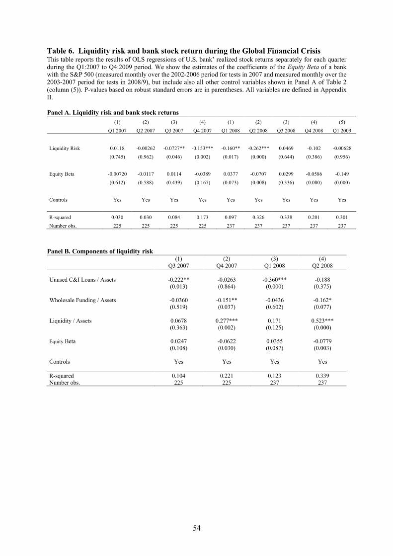
54

Table 6. Liquidity risk and bank stock return during the Global Financial Crisis This table reports the results of OLS regressions of U.S. bank’ realized stock returns separately for each quarter during the Q1:2007 to Q4:2009 period. We show the estimates of the coefficients of the Equity Beta of a bank with the S&P 500 (measured monthly over the 2002-2006 period for tests in 2007 and measured monthly over the 2003-2007 period for tests in 2008/9), but include also all other control variables shown in Panel A of Table 2 (column (5)). P-values based on robust standard errors are in parentheses. All variables are defined in Appendix II. Panel A. Liquidity risk and bank stock returns (1) (2) (3) (4) (1) (2) (3) (4) (5)

Q1 2007 Q2 2007 Q3 2007 Q4 2007 Q1 2008 Q2 2008 Q3 2008 Q4 2008 Q1 2009

Liquidity Risk 0.0118 -0.00262 -0.0727** -0.153*** -0.160** -0.262*** 0.0469 -0.102 -0.00628

(0.745) (0.962) (0.046) (0.002) (0.017) (0.000) (0.644) (0.386) (0.956)

Equity Beta -0.00720 -0.0117 0.0114 -0.0389 0.0377 -0.0707 0.0299 -0.0586 -0.149

(0.612) (0.588) (0.439) (0.167) (0.073) (0.008) (0.336) (0.080) (0.000)

Controls Yes Yes Yes Yes Yes Yes Yes Yes Yes

R-squared 0.030 0.030 0.084 0.173 0.097 0.326 0.338 0.201 0.301

Number obs. 225 225 225 225 237 237 237 237 237

Panel B. Components of liquidity risk (1) (2) (3) (4) Q3 2007 Q4 2007 Q1 2008 Q2 2008 Unused C&I Loans / Assets -0.222** -0.0263 -0.360*** -0.188 (0.013) (0.864) (0.000) (0.375) Wholesale Funding / Assets -0.0360 -0.151** -0.0436 -0.162* (0.519) (0.037) (0.602) (0.077) Liquidity / Assets 0.0678 0.277*** 0.171 0.523*** (0.363) (0.002) (0.125) (0.000) Equity Beta 0.0247 -0.0622 0.0355 -0.0779 (0.108) (0.030) (0.087) (0.003) Controls Yes Yes Yes Yes R-squared 0.104 0.221 0.123 0.339 Number obs. 225 225 237 237

55

Table 7. Understanding the mechanisms: Funding versus capital This table reports the results of OLS regressions of U.S. bank’ realized stock returns during the 1/1/2020 to 3/23/2020 period on Net Drawdowns (column (1)) and Gross Drawdowns (column (2)) and control variables. Net Drawdowns are defined as the change in a bank’s off balance sheet unused C&I loan commitments minus the change in deposits (all measured during Q1 2020) relative to total assets. Gross Drawdowns is the percentage change in a bank’s off-balance sheet unused C&I loan commitments (measured during Q1 2020). Column (4) includes an interaction term of Gross Drawdowns with Capital Buffer. Column (5) includes an interaction term of Net Drawdowns with Capital Buffer. In column (6), we use the change in bank deposits (Change Deposits) instead of Net Drawdowns. Column (7) adds SRISK/Assets as additional control. SRISK is only available for banks in the vlab database. These regressions include a dummy for banks for whom we do not find SRISK (unreported). Control variables as in column (5) in Panel A of Table 2 are included. P-values based on robust standard errors are in parentheses. All variables are defined in Appendix II. (1) (2) (3) (4) (5) (6) (7) Net Drawdowns 0.0926 0.219 0.128 0.133 0.0866

(0.885) (0.736) (0.844) (0.815) (0.889) Gross Drawdowns -4.457** -4.593** -3.929** -4.485** -4.276* -4.172**

(0.034) (0.023) (0.044) (0.026) (0.052) (0.046) Change Deposits / Assets -0.0697

(0.904) Gross Drawdowns x Capital Buffer 1.588*

(0.084) Net Drawdowns x Capital Buffer -0.109

(0.688) Change Deposits / Assets x Capital Buffer 0.175

(0.516) SRISK / Assets -6.706*

(0.071) Capital Buffer -1.442 -0.759 -0.944

(0.164) (0.415) (0.343) Controls Yes Yes Yes Yes Yes Yes Yes R-squared 0.353 0.378 0.379 0.393 0.381 0.383 0.424 Number obs. 127 127 127 127 127 127 127

56

Table 8. Implications for bank lending during the COVID-19 pandemic This table provides results of difference-in-differences regressions of the change in amount/number of loan issuance pre- and post-COVID-19 on credit line drawdowns. The analysis is based on data on firm-bank-loan type level between Jan 2019 October 2020 that is collapsed to a pre- and post-COVID-19 period (post is denoted as the period starting 4/1/2020). Panel A (B) shows the results using gross (net) drawdowns. The dependent variables are the natural log of 1 + the loan amount or the natural log of 1 + the number of loans issued. Columns (1)-(2) controls for the demand side with borrower fixed effects; column (3) additionally controls for the supply side with borrower x bank fixed effects; and column (4) additionally controls for tranche type effects with borrower x bank x tranche-type fixed effects. Detailed variable definitions can be found Appendix A. Standard errors are clustered at level of the fixed effect in each column. ***, **, * denote significance at the 1%, 5% and 10% level, respectively. All variables are defined in Appendix II. Panel A. Loan amount (1) (2) (3) (4) (5) Term Loans Credit Lines Post x Gross Drawdowns -15.69*** -8.651 -16.35* -3.129

(0.001) (0.117) (0.070) (0.657) Post x Net Drawdowns -5.676*** -4.267** -5.232 -4.099*

(0.001) (0.028) (0.141) (0.078) Post -2.270*** -2.758*** -2.544*** -2.290*** -2.710***

(0.000) (0.000) (0.000) (0.000) (0.000) Borrower x Bank x Loan Type FE Yes Yes Yes Borrower x Bank FE Yes Yes R-squared 0.200 0.200 0.200 0.186 0.208 Number obs. 17944 17944 17944 5770 12174

Panel B. Number of loans (1) (2) (3) (4) (5) Term Loans Credit Lines Post x Gross Drawdowns -2.609*** -1.710** -2.315* -1.086

(0.000) (0.040) (0.067) (0.323) Post x Net Drawdowns -0.824*** -0.545** -0.741 -0.548*

(0.001) (0.048) (0.137) (0.098) Post -0.342*** -0.419*** -0.377*** -0.315*** -0.416***

(0.000) (0.000) (0.000) (0.000) (0.000) Borrower x Bank x Loan Type FE Yes Yes Yes Borrower x Bank FE Yes Yes R-squared 0.223 0.223 0.223 0.189 0.240 Number obs. 17944 17944 17944 5770 12174

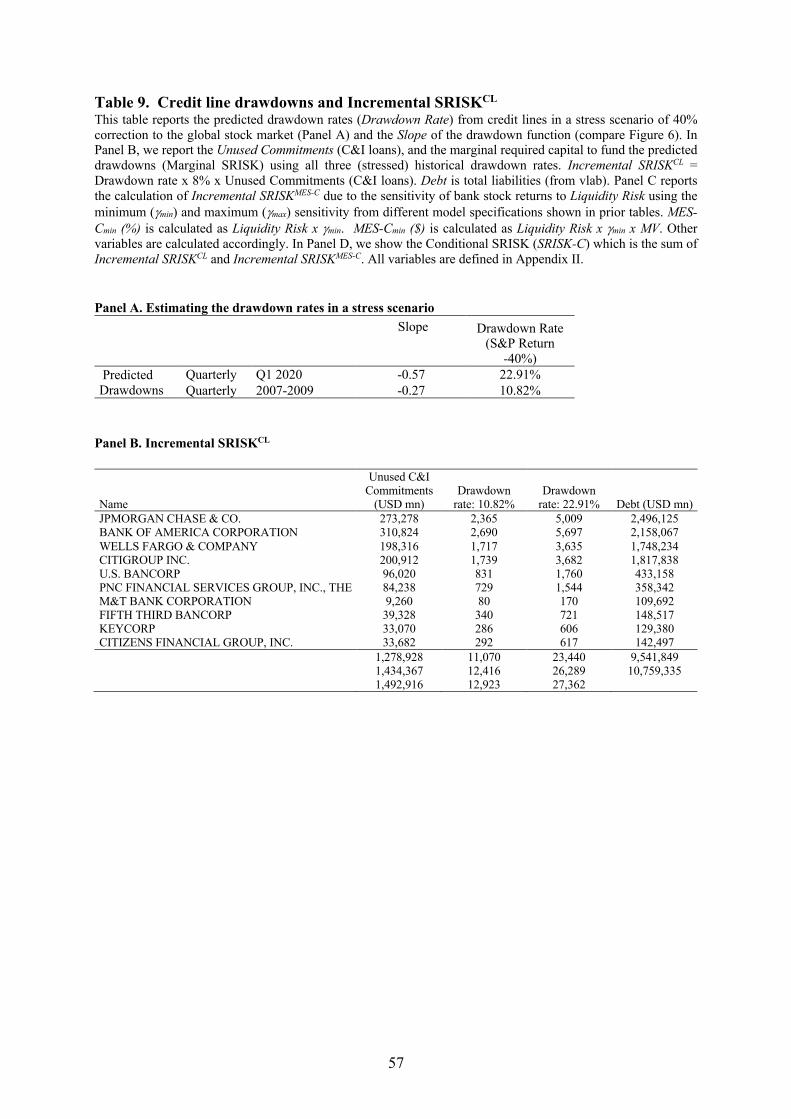
57

Table 9. Credit line drawdowns and Incremental SRISKCL This table reports the predicted drawdown rates (Drawdown Rate) from credit lines in a stress scenario of 40% correction to the global stock market (Panel A) and the Slope of the drawdown function (compare Figure 6). In Panel B, we report the Unused Commitments (C&I loans), and the marginal required capital to fund the predicted drawdowns (Marginal SRISK) using all three (stressed) historical drawdown rates. Incremental SRISKCL = Drawdown rate x 8% x Unused Commitments (C&I loans). Debt is total liabilities (from vlab). Panel C reports the calculation of Incremental SRISKMES-C due to the sensitivity of bank stock returns to Liquidity Risk using the minimum (gmin) and maximum (gmax) sensitivity from different model specifications shown in prior tables. MES-Cmin (%) is calculated as Liquidity Risk x gmin. MES-Cmin ($) is calculated as Liquidity Risk x gmin x MV. Other variables are calculated accordingly. In Panel D, we show the Conditional SRISK (SRISK-C) which is the sum of Incremental SRISKCL and Incremental SRISKMES-C. All variables are defined in Appendix II. Panel A. Estimating the drawdown rates in a stress scenario Slope Drawdown Rate (S&P Return -40%) Predicted Drawdowns

Quarterly Q1 2020 -0.57 22.91% Quarterly 2007-2009 -0.27 10.82%

Panel B. Incremental SRISKCL

Name

Unused C&I Commitments

(USD mn) Drawdown

rate: 10.82% Drawdown

rate: 22.91% Debt (USD mn) JPMORGAN CHASE & CO. 273,278 2,365 5,009 2,496,125 BANK OF AMERICA CORPORATION 310,824 2,690 5,697 2,158,067 WELLS FARGO & COMPANY 198,316 1,717 3,635 1,748,234 CITIGROUP INC. 200,912 1,739 3,682 1,817,838 U.S. BANCORP 96,020 831 1,760 433,158 PNC FINANCIAL SERVICES GROUP, INC., THE 84,238 729 1,544 358,342 M&T BANK CORPORATION 9,260 80 170 109,692 FIFTH THIRD BANCORP 39,328 340 721 148,517 KEYCORP 33,070 286 606 129,380 CITIZENS FINANCIAL GROUP, INC. 33,682 292 617 142,497

1,278,928 11,070 23,440 9,541,849 1,434,367 12,416 26,289 10,759,335

1,492,916 12,923 27,362

58

Panel C. Incremental SRISKLRMESC Incremental SRISK LRMESC Name MV LRMES Liquidity Risk gmin gmax LRMESCmin LRMESCmax LRMESC

min LRMESCmax

JPMORGAN CHASE & CO. 437,226 43.4% 20.3% -0.34 -0.54 6.9% 10.9% 30,276 47,766 BANK OF AMERICA CORPORATION 316,808 45.9% 25.7% -0.34 -0.54 8.8% 13.8% 27,761 43,799 WELLS FARGO & COMPANY 227,540 44.9% 24.2% -0.34 -0.54 8.2% 13.0% 18,768 29,610 CITIGROUP INC. 174,415 47.3% 37.1% -0.34 -0.54 12.6% 19.9% 22,047 34,784 U.S. BANCORP 92,603 36.6% 46.3% -0.34 -0.54 15.8% 24.9% 14,631 23,084 PNC FINANCIAL SERVICES GROUP, INC., THE 69,945 40.1% 39.9% -0.34 -0.54 13.6% 21.5% 9,514 15,011 M&T BANK CORPORATION 22,400 38.7% 22.6% -0.34 -0.54 7.7% 12.1% 1,724 2,720 FIFTH THIRD BANCORP 21,815 51.1% 29.9% -0.34 -0.54 10.2% 16.1% 2,222 3,506 KEYCORP 19,936 45.2% 41.7% -0.34 -0.54 14.2% 22.4% 2,834 4,472 CITIZENS FINANCIAL GROUP, INC. 17,654 48.3% 46.1% -0.34 -0.54 15.7% 24.8% 2,772 4,374 Total (Top 10 Banks) 1,400,341 132,550 209,126 Total (Vlab Banks) 1,601,754 149,543 235,935 Total (All Sample Banks) 1,756,619 158,024 249,316

Panel D. SRISKC SRISK (Q4 2019) SRISKC

min SRISKCmax

w/o neg w/ neg Name SRISK SRISK JPMORGAN CHASE & CO. 0 -27,848 32,641 52,775 BANK OF AMERICA CORPORATION 14,898 14,898 30,452 49,496 WELLS FARGO & COMPANY 24,425 24,425 20,485 33,245 CITIGROUP INC. 60,887 60,887 23,786 38,467 U.S. BANCORP 0 -19,352 15,462 24,843 PNC FINANCIAL SERVICES GROUP, INC., THE 0 -9,895 10,243 16,555 M&T BANK CORPORATION 0 -3,862 1,804 2,890 FIFTH THIRD BANCORP 2,067 2,067 2,562 4,227 KEYCORP 299 299 3,121 5,078 CITIZENS FINANCIAL GROUP, INC. 3,005 3,005 3,064 4,991 Total (Top 10 Banks) 105,581 44,623 143,621 232,566 Total (Vlab Banks) 111,135 36,680 161,958 262,224 Total (All Sample Banks) 170,947 276,678

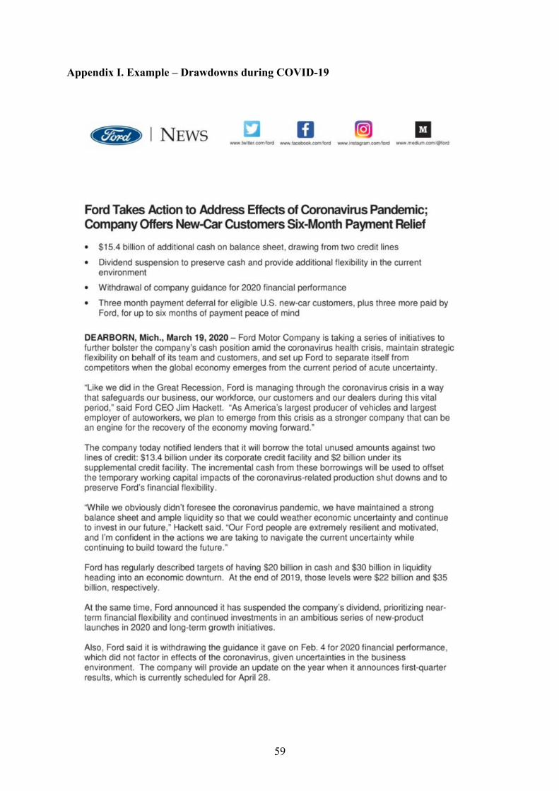
59

Appendix I. Example – Drawdowns during COVID-19

60

Appendix II. Variable definitions

Variable name Definition Source Assets Total Assets Call Reports Capital Buffer Difference between a bank’s equity-asset ratio and the cross-sectional average of the equity-asset-ratio of all sample

banks in Q4 2019 Call Reports

Consumer Loans / Assets Consumer loans (%Assets) Call Reports Credit Card Commitments / Assets Unused credit card commitments (%Assets) Call Reports Credit Lines Indicator if loan type within list: Dealscan Cumulative Total Drawdowns Natural logarithm of the realized daily cumulative credit line drawdowns across all firms 8-K Cumulative BBB Drawdowns Natural logarithm of the realized daily cumulative credit line drawdowns across all BBB-rated firms 8-K Cumulative NonIG Drawdowns Natural logarithm of the realized daily cumulative credit line drawdowns across all NonIG rated firms 8-K Cumulative Not Rated Drawdowns Natural logarithm of the realized daily cumulative credit line drawdowns across all unrated firms 8-K Current Primary Dealer Indicator Indicator = 1 if bank is current primary dealer bank (https://www.newyorkfed.org/markets/primarydealers#primary-

dealers) NY Fed

Debt Market value of bank liabilities (12/31/2019) Vlab Deposits / Assets Deposits (%Assets) Call Reports Deposits / Loans Deposits (%Loans) Call Reports Derivatives / Assets Interest rate, exchange rat and credit derivatives (% Assets) Call Reports Distance-to-Default Mean(ROA+CAR)/volatility(ROA) where CAR is the capital-to-asset ratio and ROA is return on assets Call Reports Drawdown Rate Sensitivity of changes in credit line drawdowns to changes in the market returns (projected in a market downturn of

40%) Capital IQ, 8-K, CRSP

Equity Beta Constructed using monthly data over the 2015 to 2019 period and the S&P 500 as market index CRSP Equity Ratio Equity (%Assets) Call Reports Gross Drawdowns Percentage change of banks’ off-balance sheet unused C&I commitments between Q4 2019 and Q1 2020 Call Reports Idiosyncratic Volatility Annualized standard deviation of the residuals from the market model CRSP Income Diversity 1 minus the absolute value of the ratio of the difference between net interest income and other operating income to total

operating income Call Reports

Incremental SRISKCL Equity capital that would be required to fund new loans based on banks’ unused commitments (CL = credit lines) at the end of Q4 2019

Call Reports

Incremental SRISKLRMESC (Marginal) equity shortfall of banks based on their end of Q4 2019 market values of equity due to effect of liquidity risk on stock returns

Call Reports

Liquidity The sum of cash, federal funds sold & reverse repos, and securities excluding MBS/ABS securities. Call Reports Liquidity Risk Unused Commitments plus Wholesale Funding minus Liquidity (% Assets) Call Reports Loan Either natural log of loan amount or natural log of 1+number of loans Dealscan Loans / Assets Total loans (%Assets) Call Reports Log(Assets) Natural log of Assets Call Reports LRMES LRMES is the Long Run Marginal Expected Shortfall, approximated in Acharya et al. (2012) as

1-e^((-18×MES)), where MES is the one-day loss expected in bank i’s return if market returns are less than -2% Call Reports

LRMESC Contingent marginal expected shortfall due to the impact of liquidity risk on bank stock returns. Call Reports, CRSP MV Market value of equity (12/31/2019) Vlab Net Drawdowns Absolute change in banks’ unused C&I commitments minus the change in deposits (% Assets) over the same period Call Reports

61

Non-Interest Income Non-interest-income (%Operating revenues) Call Reports NPL / Loans Non-performing loans (%Loans) Call Reports Oil Exposure / Assets Sum of a bank’s active loan exposures to oil & gas firms (%Assets) Dealscan Other Sectoral Exposures / Assets Sum of a bank’s active loan exposures to the retail, leisure, and hotel & gaming industry (%Assets) Dealscan Post Post is defined as the period starting April 1, 2020

Real Estate Beta Slope of the regression of weekly excess stock returns on the Fama and French real estate industry excess return in a regression that controls for the MSCI World excess return

CRSP

Return 1/1-3/23/2020 Cumulative stock return from January 1 to March 23, 2020; log excess returns are calculated as the log(1 + r - rf), where r is the simple daily return (based on the daily closing price, adjusted for total return factor and daily adjustment factor), and rf is the 1-month daily Treasury-bill rate

CRSP

Return January 2020 Cumulative stock return from January 1 to January 31, 2020 CRSP Return February 2020 Cumulative stock return from February 1 to February 29, 2020 CRSP Return 3/1-3/23/2020 Cumulative stock return from March 1 to March 23, 2020 CRSP Return April 2020 Cumulative stock return from 01.04.-30.04.2020 CRSP Return May 2020 Cumulative stock return from 01.05.-31.05.2020 CRSP Return June 2020 Cumulative stock return from 01.06.-30.06.2020 CRSP ROA Return on assets: Net Income / Assets Call Reports S&P 500 Return (Daily) excess return of the S&P 500 index; log excess returns are calculated as the log(1 + r - rf), where r is the simple

daily return (based on the daily closing price, adjusted for total return factor and daily adjustment factor), and rf is the 1-month daily Treasury-bill rate

CRSP

SRISK Bank capital shortfall in a systemic crisis as in Acharya et al. (2012) Vlab SRISK/Assets SRISK scaled by total assets Vlab and Call Reports SRISKC Incremental SRISKCL + Incremental SRISKLRMES-C Call Reports Term Loan Indicator if loan type within list: Dealscan Unused C&I Commitments Unused C&I credit lines Call Reports Unused Commitments The sum of credit lines secured by 1-4 family homes, secured and unsecured commercial real estate credit lines,

commitments related to securities underwriting, commercial letter of credit, and other credit lines (which includes commitments to extend credit through overdraft facilities or commercial lines of credit)

Call Reports

Wholesale Funding The sum of large time deposits, deposited booked in foreign offices, subordinated debt and debentures, gross federal funds purchased, repos and other borrowed money.

Call Reports

Why did bank stocks crash during COVID-19?

Viral V. Acharya† Robert Engle‡ Sascha Steffen*

March 8, 2021

Online Appendix

(Not for publication)

†NYU Stern School of Business, 44 West Fourth Street, Suite 9-10, New York, NY 10012-1126, Email: [email protected], Tel: +1 212 998 0354. ‡NYU Stern School of Business, 44 West Fourth Street, Suite 9-62, New York, NY 10012-1126, Email: [email protected], Tel: +1 212 998 0710. *Frankfurt School of Finance & Management, Adickesallee 32-34, 60323 Frankfurt, Germany, Email: [email protected], Tel: +49 (0)69 154008-794.

63

Table of Content

A Industry exposure and performance

Figure A.1. Industry performance during COVID-19

Figure A.2. Event study around the oil price shock (9 March 2020)

B Reversal of credit line drawdowns

Table B.1 Descriptive statistics of firm’s capital structure (Q4 2019 vs. Q3 2020)

Table B.2 Descriptive statistics of firm’s capital structure (quarterly since Q4 2019)

Figure B.1 Preference for cash

C SRISK

Table C.1 SRISK-C using only unused C&I loans

D Alternative liquidity proxies

Figure D.1. Dynamic LMI during COVID-19

Table D.1. Liquidity risk measures and pricing of drawdown options

Table D.2. Pricing of drawdown options in credit line fees

E Pricing of drawdown options in credit line fees

Table E.1. Pricing of drawdown options in credit line fees

64

Appendix A. Industry exposure and performance After the oil price shock on March 9, 2020, the market performance of the oil & gas sector

considerably deteriorated. Panel A of Figure A.1. shows the performance of this sector vis-à-

vis other sectors directly affected by the pandemic (i.e., retail, leisure and hotel & gaming)

using returns from loans traded in the secondary market in these sectors. While the returns in

the loan market declined substantially in all sectors, loan return of oil & gas and mining firms

significantly underperformed the other sectors even after the announcement of the interventions

by the Fed on March 23, 2020.

Panel B of Figure A.1. show the time-series of oil-price volatility using the CVOX oil

price volatility index. While oil price volatility increases episodically during economic

downturns (e.g., during the global financial crisis (GFC), i.e., the 2007 to 2009 period), the

European sovereign debt crisis (2011-2012), and the oil & gas crisis in 2015-2016), volatility

has increased by more than 6 times (to over 100% on an annualized basis) around March 9th,

2020 and energy stocks crashed.

Banks are heavily exposed through loans provided to this sector. Both bank exposures

and the riskiness of energy firm balance sheets have risen steadily in the recent years. We

measure a bank’s exposure to the oil sector using all active loans at the end of Q4:2019 and

scaled by Tier 1 capital.

In addition to the tests in the main paper, we perform an event study using a 2-day

window around 9 March 2020 and plot banks’ 2-day beta adjusted return (= "! − $!""&$)23 on

banks’ exposure to the oil & gas sector scaled by Tier 1 capital (Figure A.2.). We find a

significant negative correlation suggesting that oil price risk is priced in bank stock returns.

23 The beta is measured pre-crisis, i.e., at the end of Q4 2019.

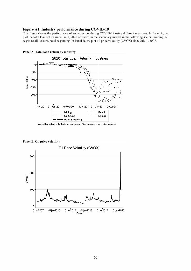
65

Figure A1. Industry performance during COVID-19 This figure shows the performance of some sectors during COVID-19 using different measures. In Panel A, we plot the total loan return since Jan 1, 2020 of traded in the secondary market in the following sectors: mining, oil & gas retail, leisure, hotel & gaming. In Panel B, we plot oil price volatility (CVOX) since July 1, 2007. Panel A. Total loan return by industry

Panel B. Oil price volatility

66

Figure A2. Event study around the oil price shock (9 March 2020) This figure plots the 2-day beta adjusted bank stock return around the oil price shock on March 9, 2002 on banks’ loan exposure to the oil & gas industry scaled by Tier 1 capital.

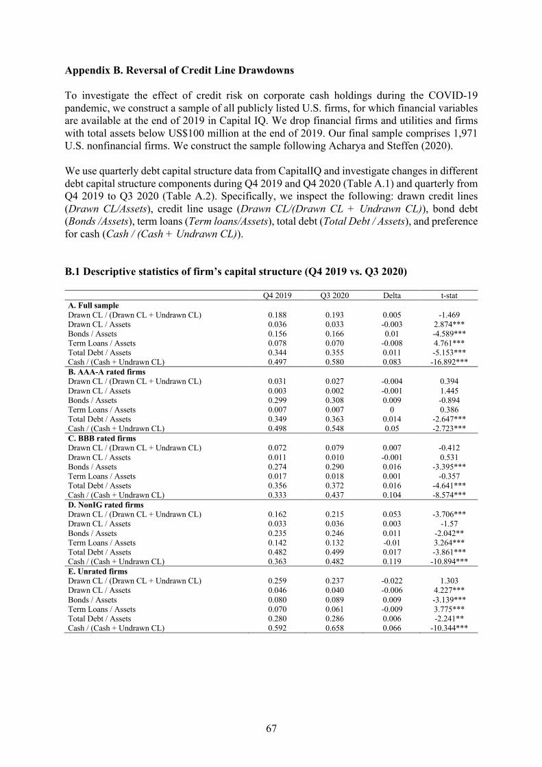
67

Appendix B. Reversal of Credit Line Drawdowns To investigate the effect of credit risk on corporate cash holdings during the COVID-19

pandemic, we construct a sample of all publicly listed U.S. firms, for which financial variables are available at the end of 2019 in Capital IQ. We drop financial firms and utilities and firms

with total assets below US$100 million at the end of 2019. Our final sample comprises 1,971 U.S. nonfinancial firms. We construct the sample following Acharya and Steffen (2020).

We use quarterly debt capital structure data from CapitalIQ and investigate changes in different

debt capital structure components during Q4 2019 and Q4 2020 (Table A.1) and quarterly from Q4 2019 to Q3 2020 (Table A.2). Specifically, we inspect the following: drawn credit lines

(Drawn CL/Assets), credit line usage (Drawn CL/(Drawn CL + Undrawn CL)), bond debt (Bonds /Assets), term loans (Term loans/Assets), total debt (Total Debt / Assets), and preference

for cash (Cash / (Cash + Undrawn CL)).

B.1 Descriptive statistics of firm’s capital structure (Q4 2019 vs. Q3 2020) Q4 2019 Q3 2020 Delta t-stat A. Full sample Drawn CL / (Drawn CL + Undrawn CL) 0.188 0.193 0.005 -1.469 Drawn CL / Assets 0.036 0.033 -0.003 2.874*** Bonds / Assets 0.156 0.166 0.01 -4.589*** Term Loans / Assets 0.078 0.070 -0.008 4.761*** Total Debt / Assets 0.344 0.355 0.011 -5.153*** Cash / (Cash + Undrawn CL) 0.497 0.580 0.083 -16.892*** B. AAA-A rated firms Drawn CL / (Drawn CL + Undrawn CL) 0.031 0.027 -0.004 0.394 Drawn CL / Assets 0.003 0.002 -0.001 1.445 Bonds / Assets 0.299 0.308 0.009 -0.894 Term Loans / Assets 0.007 0.007 0 0.386 Total Debt / Assets 0.349 0.363 0.014 -2.647*** Cash / (Cash + Undrawn CL) 0.498 0.548 0.05 -2.723*** C. BBB rated firms Drawn CL / (Drawn CL + Undrawn CL) 0.072 0.079 0.007 -0.412 Drawn CL / Assets 0.011 0.010 -0.001 0.531 Bonds / Assets 0.274 0.290 0.016 -3.395*** Term Loans / Assets 0.017 0.018 0.001 -0.357 Total Debt / Assets 0.356 0.372 0.016 -4.641*** Cash / (Cash + Undrawn CL) 0.333 0.437 0.104 -8.574*** D. NonIG rated firms Drawn CL / (Drawn CL + Undrawn CL) 0.162 0.215 0.053 -3.706*** Drawn CL / Assets 0.033 0.036 0.003 -1.57 Bonds / Assets 0.235 0.246 0.011 -2.042** Term Loans / Assets 0.142 0.132 -0.01 3.264*** Total Debt / Assets 0.482 0.499 0.017 -3.861*** Cash / (Cash + Undrawn CL) 0.363 0.482 0.119 -10.894*** E. Unrated firms Drawn CL / (Drawn CL + Undrawn CL) 0.259 0.237 -0.022 1.303 Drawn CL / Assets 0.046 0.040 -0.006 4.227*** Bonds / Assets 0.080 0.089 0.009 -3.139*** Term Loans / Assets 0.070 0.061 -0.009 3.775*** Total Debt / Assets 0.280 0.286 0.006 -2.241** Cash / (Cash + Undrawn CL) 0.592 0.658 0.066 -10.344***

68

Table B.2. Descriptive statistics of firm’s capital structure (Q4 2019 to Q3 2020) Panel A. Full sample Variable Mean Std dev Min Max Drawn CL / (Drawn CL + Undrawn CL) - Q4 2019 0.188 0.269 0.000 1.000 Drawn CL / (Drawn CL + Undrawn CL) - Q1 2020 0.381 0.353 0.000 1.000 Drawn CL / (Drawn CL + Undrawn CL) - Q2 2020 0.277 0.332 0.000 1.000 Drawn CL / (Drawn CL + Undrawn CL) - Q3 2020 0.193 0.288 0.000 1.000 Drawn CL / Assets - Q4 2019 0.036 0.073 0.000 0.355 Drawn CL / Assets - Q1 2020 0.058 0.086 0.000 0.400 Drawn CL / Assets - Q2 2020 0.046 0.081 0.000 0.396 Drawn CL / Assets - Q3 2020 0.033 0.069 0.000 0.340 Bonds / Assets - Q4 2019 0.156 0.192 0.000 0.909 Bonds / Assets - Q1 2020 0.158 0.194 0.000 0.923 Bonds / Assets - Q2 2020 0.167 0.198 0.000 0.873 Bonds / Assets - Q3 2020 0.166 0.198 0.000 0.855 Term Loans / Assets - Q4 2019 0.078 0.134 0.000 0.645 Term Loans / Assets - Q1 2020 0.078 0.132 0.000 0.617 Term Loans / Assets - Q2 2020 0.078 0.131 0.000 0.598 Term Loans / Assets - Q3 2020 0.070 0.124 0.000 0.565 Total Debt / Assets - Q4 2019 0.344 0.229 0.002 1.134 Total Debt / Assets - Q1 2020 0.370 0.240 0.002 1.180 Total Debt / Assets - Q2 2020 0.368 0.243 0.002 1.242 Total Debt / Assets - Q3 2020 0.355 0.241 0.002 1.228 Cash / (Cash + Undrawn CL) - Q4 2019 0.497 0.344 0.002 1.000 Cash / (Cash + Undrawn CL) - Q1 2020 0.608 0.333 0.005 1.000 Cash / (Cash + Undrawn CL) - Q2 2020 0.593 0.329 0.004 1.000 Cash / (Cash + Undrawn CL) - Q3 2020 0.580 0.331 0.006 1.000

Panel B. AAA-A rated firms Variable Mean Std dev Min Max Drawn CL / (Drawn CL + Undrawn CL) - Q4 2019 0.031 0.113 0.000 0.911 Drawn CL / (Drawn CL + Undrawn CL) - Q1 2020 0.156 0.290 0.000 1.000 Drawn CL / (Drawn CL + Undrawn CL) - Q2 2020 0.069 0.195 0.000 0.958 Drawn CL / (Drawn CL + Undrawn CL) - Q3 2020 0.027 0.085 0.000 0.445 Drawn CL / Assets - Q4 2019 0.003 0.014 0.000 0.125 Drawn CL / Assets - Q1 2020 0.013 0.028 0.000 0.142 Drawn CL / Assets - Q2 2020 0.007 0.023 0.000 0.147 Drawn CL / Assets - Q3 2020 0.002 0.008 0.000 0.053 Bonds / Assets - Q4 2019 0.299 0.154 0.000 0.754 Bonds / Assets - Q1 2020 0.308 0.151 0.000 0.781 Bonds / Assets - Q2 2020 0.319 0.138 0.011 0.779 Bonds / Assets - Q3 2020 0.308 0.133 0.000 0.770 Term Loans / Assets - Q4 2019 0.007 0.017 0.000 0.108 Term Loans / Assets - Q1 2020 0.008 0.019 0.000 0.145 Term Loans / Assets - Q2 2020 0.007 0.013 0.000 0.058 Term Loans / Assets - Q3 2020 0.007 0.013 0.000 0.060 Total Debt / Assets - Q4 2019 0.349 0.145 0.046 0.753 Total Debt / Assets - Q1 2020 0.369 0.147 0.045 0.757 Total Debt / Assets - Q2 2020 0.376 0.135 0.062 0.757 Total Debt / Assets - Q3 2020 0.363 0.130 0.057 0.754 Cash / (Cash + Undrawn CL) - Q4 2019 0.498 0.322 0.002 1.000 Cash / (Cash + Undrawn CL) - Q1 2020 0.585 0.308 0.005 1.000 Cash / (Cash + Undrawn CL) - Q2 2020 0.564 0.296 0.004 1.000 Cash / (Cash + Undrawn CL) - Q3 2020 0.548 0.304 0.006 1.000

69

Panel C. BBB rated firms Variable Mean Std dev Min Max Drawn CL / (Drawn CL + Undrawn CL) - Q4 2019 0.072 0.165 0.000 1.000 Drawn CL / (Drawn CL + Undrawn CL) - Q1 2020 0.235 0.285 0.000 1.000 Drawn CL / (Drawn CL + Undrawn CL) - Q2 2020 0.129 0.241 0.000 1.000 Drawn CL / (Drawn CL + Undrawn CL) - Q3 2020 0.079 0.182 0.000 1.000 Drawn CL / Assets - Q4 2019 0.011 0.039 0.000 0.344 Drawn CL / Assets - Q1 2020 0.030 0.053 0.000 0.400 Drawn CL / Assets - Q2 2020 0.019 0.046 0.000 0.396 Drawn CL / Assets - Q3 2020 0.010 0.026 0.000 0.240 Bonds / Assets - Q4 2019 0.274 0.136 0.000 0.909 Bonds / Assets - Q1 2020 0.279 0.138 0.000 0.923 Bonds / Assets - Q2 2020 0.292 0.141 0.000 0.873 Bonds / Assets - Q3 2020 0.290 0.146 0.000 0.855 Term Loans / Assets - Q4 2019 0.017 0.035 0.000 0.203 Term Loans / Assets - Q1 2020 0.022 0.042 0.000 0.286 Term Loans / Assets - Q2 2020 0.021 0.038 0.000 0.221 Term Loans / Assets - Q3 2020 0.018 0.036 0.000 0.232 Total Debt / Assets - Q4 2019 0.356 0.145 0.048 1.001 Total Debt / Assets - Q1 2020 0.381 0.148 0.075 1.034 Total Debt / Assets - Q2 2020 0.382 0.148 0.064 1.040 Total Debt / Assets - Q3 2020 0.372 0.145 0.054 1.017 Cash / (Cash + Undrawn CL) - Q4 2019 0.333 0.254 0.002 1.000 Cash / (Cash + Undrawn CL) - Q1 2020 0.439 0.269 0.015 1.000 Cash / (Cash + Undrawn CL) - Q2 2020 0.446 0.267 0.004 1.000 Cash / (Cash + Undrawn CL) - Q3 2020 0.437 0.268 0.006 1.000

Panel D. NonIG rated firms Variable Mean Std dev Min Max Drawn CL / (Drawn CL + Undrawn CL) - Q4 2019 0.162 0.241 0.000 1.000 Drawn CL / (Drawn CL + Undrawn CL) - Q1 2020 0.443 0.353 0.000 1.000 Drawn CL / (Drawn CL + Undrawn CL) - Q2 2020 0.310 0.335 0.000 1.000 Drawn CL / (Drawn CL + Undrawn CL) - Q3 2020 0.215 0.301 0.000 1.000 Drawn CL / Assets - Q4 2019 n 0.033 0.066 0.000 0.355 Drawn CL / Assets - Q1 2020 0.067 0.078 0.000 0.400 Drawn CL / Assets - Q2 2020 0.048 0.071 0.000 0.396 Drawn CL / Assets - Q3 2020 0.036 0.068 0.000 0.340 Bonds / Assets - Q4 2019 0.235 0.187 0.000 0.909 Bonds / Assets - Q1 2020 0.236 0.190 0.000 0.923 Bonds / Assets - Q2 2020 0.252 0.199 0.000 0.873 Bonds / Assets - Q3 2020 0.246 0.199 0.000 0.855 Term Loans / Assets - Q4 2019 0.142 0.157 0.000 0.645 Term Loans / Assets - Q1 2020 0.141 0.157 0.000 0.617 Term Loans / Assets - Q2 2020 0.141 0.156 0.000 0.598 Term Loans / Assets - Q3 2020 0.132 0.150 0.000 0.565 Total Debt / Assets - Q4 2019 0.482 0.198 0.051 1.134 Total Debt / Assets - Q1 2020 0.518 0.205 0.059 1.180 Total Debt / Assets - Q2 2020 0.518 0.215 0.058 1.242 Total Debt / Assets - Q3 2020 0.499 0.217 0.053 1.228 Cash / (Cash + Undrawn CL) - Q4 2019 0.363 0.263 0.002 1.000 Cash / (Cash + Undrawn CL) - Q1 2020 0.540 0.320 0.005 1.000 Cash / (Cash + Undrawn CL) - Q2 2020 0.500 0.311 0.004 1.000 Cash / (Cash + Undrawn CL) - Q3 2020 0.482 0.302 0.006 1.000

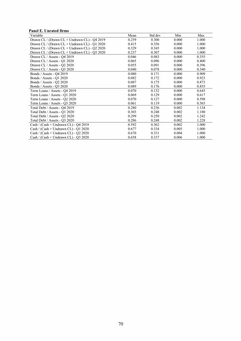
70

Panel E. Unrated firms Variable Mean Std dev Min Max Drawn CL / (Drawn CL + Undrawn CL) - Q4 2019 0.259 0.300 0.000 1.000 Drawn CL / (Drawn CL + Undrawn CL) - Q1 2020 0.415 0.356 0.000 1.000 Drawn CL / (Drawn CL + Undrawn CL) - Q2 2020 0.329 0.345 0.000 1.000 Drawn CL / (Drawn CL + Undrawn CL) - Q3 2020 0.237 0.307 0.000 1.000 Drawn CL / Assets - Q4 2019 0.046 0.083 0.000 0.355 Drawn CL / Assets - Q1 2020 0.065 0.096 0.000 0.400 Drawn CL / Assets - Q2 2020 0.055 0.091 0.000 0.396 Drawn CL / Assets - Q3 2020 0.040 0.078 0.000 0.340 Bonds / Assets - Q4 2019 0.080 0.171 0.000 0.909 Bonds / Assets - Q1 2020 0.082 0.172 0.000 0.923 Bonds / Assets - Q2 2020 0.087 0.175 0.000 0.873 Bonds / Assets - Q3 2020 0.089 0.176 0.000 0.855 Term Loans / Assets - Q4 2019 0.070 0.132 0.000 0.645 Term Loans / Assets - Q1 2020 0.069 0.129 0.000 0.617 Term Loans / Assets - Q2 2020 0.070 0.127 0.000 0.598 Term Loans / Assets - Q3 2020 0.061 0.119 0.000 0.565 Total Debt / Assets - Q4 2019 0.280 0.236 0.002 1.134 Total Debt / Assets - Q1 2020 0.303 0.248 0.002 1.180 Total Debt / Assets - Q2 2020 0.299 0.250 0.002 1.242 Total Debt / Assets - Q3 2020 0.286 0.248 0.002 1.228 Cash / (Cash + Undrawn CL) - Q4 2019 0.592 0.362 0.002 1.000 Cash / (Cash + Undrawn CL) - Q1 2020 0.677 0.334 0.005 1.000 Cash / (Cash + Undrawn CL) - Q2 2020 0.670 0.331 0.004 1.000 Cash / (Cash + Undrawn CL) - Q3 2020 0.658 0.337 0.006 1.000

71

Figure B.1. Preference for cash This figure shows the median Cash / (Cash + Undrawn CL) ratio (panel B) of U.S. nonfinancial firms over the Q1 2018 to Q3 2020 period.

Preference for cash has increased / remained high during the 3 quarters in 2020, particularly

of lower rated and unrated firms.

72

Appendix C – SRISK-C using only unused C&I loans

In Online Appendix C, we calculate SRISK-C but use only unused C&I loans (and the

estimated coffients) . Everything else is as in Table 9 of the main paper.

73

Table B.1 Incremental SRISKLRMES-C Panel A reports the calculation of Incremental SRISKMES-C due to the sensitivity of bank stock returns to Unused C&I Credit Lines using the minimum (gmin) and maximum (gmax) sensitivity from different model specifications shown in prior tables. MES-Cmin (%) is calculated as Liquidity Risk x gmin. MES-Cmin ($) is calculated as Liquidity Risk x gmin x MV. Other variables are calculated accordingly. In Panel B, we show the Conditional SRISK (SRISK-C) which is the sum of Incremental SRISKCL and Incremental SRISKMES-C. All variables are defined in Appendix I. Panel A. Incremental SRISK LRMES-C

MV LRMES Liquidity Risk gmin gmax LRMES-Cmin LRMES-Cmax LRMES-Cmin LRMES-Cmax

JPMORGAN CHASE & CO. 437,226 43.4% 20.3% -1.012 -1.383 10.3% 14.1% 44,995 61,490 BANK OF AMERICA CORPORATION 316,808 45.9% 25.7% -1.012 -1.383 12.9% 17.7% 40,941 55,950 WELLS FARGO & COMPANY 227,540 44.9% 24.2% -1.012 -1.383 10.4% 14.2% 23,691 32,377 CITIGROUP INC. 174,415 47.3% 37.1% -1.012 -1.383 10.4% 14.2% 18,175 24,838 U.S. BANCORP 92,603 36.6% 46.3% -1.012 -1.383 19.6% 26.8% 18,163 24,822 PNC FINANCIAL SERVICES GROUP, INC., THE 69,945 40.1% 39.9% -1.012 -1.383 20.8% 28.4% 14,530 19,857 M&T BANK CORPORATION 22,400 38.7% 22.6% -1.012 -1.383 7.8% 10.7% 1,751 2,393 FIFTH THIRD BANCORP 21,815 51.1% 29.9% -1.012 -1.383 23.5% 32.1% 5,126 7,006 KEYCORP 19,936 45.2% 41.7% -1.012 -1.383 23.0% 31.4% 4,583 6,264 CITIZENS FINANCIAL GROUP, INC. 17,654 48.3% 46.1% -1.012 -1.383 20.5% 28.0% 3,623 4,951 Total (Top 10 Banks) 1,400,341 175,579 239,946 Total (Vlab Banks) 1,601,754 197,984 270,565 Total (All Sample Banks) 1,756,619 207,978 284,223

74

Panel B. SRISK-C Name SRISK (Q4 2019) SRISK-Cmin SRISK-Cmax

w/o neg SRISK

w/ neg SRISK

JPMORGAN CHASE & CO. 0 -27,848 51,604 73,392 BANK OF AMERICA CORPORATION 14,898 14,898 48,458 69,487 WELLS FARGO & COMPANY 24,425 24,425 28,487 41,014 CITIGROUP INC. 60,887 60,887 23,034 33,588 U.S. BANCORP 0 -19,352 20,485 29,003 PNC FINANCIAL SERVICES GROUP, INC., THE 0 -9,895 16,567 23,525 M&T BANK CORPORATION 0 -3,862 1,975 2,796 FIFTH THIRD BANCORP 2,067 2,067 6,077 8,718 KEYCORP 299 299 5,383 7,704 CITIZENS FINANCIAL GROUP, INC. 3,005 3,005 4,438 6,418 Total (Top 10 Banks) 105,581 44,623 206,508 295,646 Total (Vlab Banks) 111,135 36,680 232,673 333,034 Total (All Sample Banks) 244,083 349,243

75

Appendix D - Discussion Finally, we discuss the robustness of our results and its extensions along several dimensions in

section 8 in the main body of the paper. (1) Alternative liquidity proxies used in the literature;

(2) pricing of contingent drawdown options through credit line fees; (3) the role of covenants

during the pandemic; and (4) repayment of credit lines after fiscal and monetary interventions.

D.1. Constructing our liquidity proxies

In Online Appendix D.1 , we discuss provide a more extensive discussion of the different

liquidity proxies used in the literature.

A. Berger and Bouwman (2009) liquidity creation measure

To replicate the Berger-Bouwman (2009) measure on liquidity creation using FR Y-9C data,

we apply the data mapping available in Berger et al. (2020).24 Individual on- and off-balance

sheet items are aggregated and weighted in line with the classification provided by Berger &

Bouwman (2009). Finally, the weighted positions are combined to the aggregate liquidity

creation measure for each bank holding company. Note that we only replicate Berger &

Bouwman’s so-called “catfat” measure, which is constructed by classifying balance sheet items

by category (see Berger & Bouwman, 2009) and includes on- as well as off-balance sheet

positions.

B. Bai et al. (2018) liquidity risk measure (LMI)

To construct the Bai et al. (2018) liquidity mismatch index (LMI), we use information provided

in the paper’s Online Appendix together with the FR Y-9C call report template for 2019Q4 to

map all balance sheet items, except deposits, to the variables in our dataset. The deposit data is

constructed in line with the approach outlined in Bai et al. (2018), using FFIEC 031 call report

data for commercial banks aggregated for the respective parent bank holding company.25

24 Berger, A.N., C.H.S. Bouwman, B. Imbierowicz and C. Rauch (2020), How are banks special? – Let me count the ways. 25 We thank Jennie Bai for detailed guidance how to construct their measure.

76

Commercial banks and bank holding companies are matched with the help of the FSSD’s

relationship table. We consider a bank holding company to be a commercial bank’s parent, if

their relationship exists at least until 31 December 2019.

In the next step, we calculate the asset and liability weights per category as indicated in

Bai et al. (2018) using the parameters and estimates provided by the authors. Accordingly,

haircut values as well as the magnitude of the Frist Principal Component used in constructing

our measure are averages taken from Bai et al. (2018). As described in the main text of the

paper, we use two different proxies for the liquidity premium μt, which is defined as the OIS -

3m Treasury Bill spread. We create two LMIs, one using liquidity conditions as of Q4 2019

(LMI – 2019) and one using the worst liquidity condition in March 2020 (LMI – 2020). We

weigh the aggregate positions with the respective asset/liability weight to calculate the liquidity

risk measure per bank holding company.

Both LMI measures are constructed as of Q4 2019. We also construct a time-series LMI

measure using a daily adjusting liquidity weight. We plot the time-series in Figure D.1. below.

Liquidity risk increases significantly in March 2020 within a few days and then returned almost

to a pre-COVID-19 level when monetary and fiscal policy measures have been implemented.

77

Figure D.1. Dynamic LMI during COVID-19 Figure D.1. plots the times-series LMI measure using a daily adjusted OIS-3m Treasury spread measure as liquidity weight.

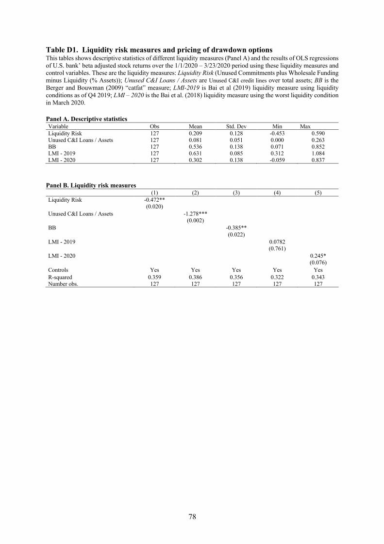
78

Table D1. Liquidity risk measures and pricing of drawdown options This tables shows descriptive statistics of different liquidity measures (Panel A) and the results of OLS regressions of U.S. bank’ beta adjusted stock returns over the 1/1/2020 – 3/23/2020 period using these liquidity measures and control variables. These are the liquidity measures: Liquidity Risk (Unused Commitments plus Wholesale Funding minus Liquidity (% Assets)); Unused C&I Loans / Assets are Unused C&I credit lines over total assets; BB is the Berger and Bouwman (2009) “catfat” measure; LMI-2019 is Bai et al (2019) liquidity measure using liquidity conditions as of Q4 2019; LMI – 2020 is the Bai et al. (2018) liquidity measure using the worst liquidity condition in March 2020. Panel A. Descriptive statistics Variable Obs Mean Std. Dev Min Max Liquidity Risk 127 0.209 0.128 -0.453 0.590 Unused C&I Loans / Assets 127 0.081 0.051 0.000 0.263 BB 127 0.536 0.138 0.071 0.852 LMI - 2019 127 0.631 0.085 0.312 1.084 LMI - 2020 127 0.302 0.138 -0.059 0.837

Panel B. Liquidity risk measures (1) (2) (3) (4) (5) Liquidity Risk -0.472**

(0.020) Unused C&I Loans / Assets -1.278***

(0.002) BB -0.385**

(0.022) LMI - 2019 0.0782

(0.761) LMI - 2020 0.245*

(0.076) Controls Yes Yes Yes Yes Yes R-squared 0.359 0.386 0.356 0.322 0.343 Number obs. 127 127 127 127 127

79

E. Pricing of drawdown options in credit line fees Do banks consider the deep out-of-the-money put option associated with aggregate drawdown

risk when setting ex-ante price terms of credit lines? We follow earlier work on the pricing of

credit lines such as Acharya et al. (2013) and Berg et al. (2015) and build a panel data set of

U.S. non-financial firms that have obtained credit lines in the primary loan market over the

2010 to 2019 period. That is, using all originated loans from the Refinitiv Dealscan database,

we keep only credit lines issued over the sample period, keep the lead arranger (following the

procedures outlined in many previous papers) and collapse the All-In-Spread-Drawn (AISD)

and the All-In-Spread-Undrawn (AISU) at their respective means to construct a firm-year-lead-

arranger level panel.

We then use the merged CRSP/Compustat database to add firm characteristics that

affect a firm’s cost of credit, in particular a firm’s equity volatility as a measure of idiosyncratic

risk and a firm’s market beta for systematic risk. Other control variables include size,

profitability, tangibility, Tobin’s Q and leverage. We source bank characteristics from call

report data including NPL/Loans, capital, non-interest income, bank size and bank profitability.

Importantly, we obtain data on banks’ aggregate risk exposure from call reports, CRSP and

vlab including Bank Equity Beta (as a measure of systematic risk), LRMES (as a measure of

downside risk), SRISK/Assets (as a measure of equity shortfall in times of a severe crisis) and

Liquidity Risk (as a measure of aggregate drawdown risk). LIBOR is included as all contracts

are floating rate and prior literature has shown that spreads and fees are sensitive to the current

level of LIBOR.

We estimate the following regression:

!"#$!,#,$ = &% + &&())*+#,#,$ + &'-./0*$ + 1(2),* + 1+2,,* + 3$ + 4- + 5!,#,$

Where ())*+#,#,$ are bank-specific aggregate risk proxies, 2),* (2,,*) are bank (firm)

characteristics, 3$ are year and 4- industry fixed effects.

80

The results are reported in Table E.1. We first show that idiosyncratic drawdown risk (measured

using a firm’s realized equity volatility over the past 12 months) and systematic drawdown risk

(measured using a firm’s stock beta) are priced in both commitment fee (AISU) and spread

(AISD). This is consistent with, for example, Acharya et al. (2013) and Berg et al. (2015).

However, while a higher Bank Beta and LRMES both somewhat increase the price of

credit lines, Liquidity Risk or Unused C&I / Assets, on average, do not. Also, SRISK / Assets,

which measures bank capital shortfall in times of aggregate market downturn, does not appear

to be priced either. In other words, banks do not appear to be considering the deep out-of-the-

money put option associated with aggregate drawdown risk when setting ex-ante price terms of

credit lines. This may partly explain their need to fund aggregate drawdown risk with equity

capital, as witnessed during the pandemic.

81

Table E.1. Pricing of drawdown options in credit line fees This table reports the results of OLS regressions of the All-In-Spread-Drawn (AISD) and the All-In-Spread-Undrawn (AISU) ratio on banks’ aggregate risk exposures including Bank Equity Beta (as a measure of systematic risk), LRMES (as a measure of downside risk; LRMES is the Long Run Marginal Expected Shortfall, approximated in Acharya et al. (2012) as 1-e^((-18×MES)), where MES is the one-day loss expected in bank i’s return if market returns are less than -2%), SRISK/Assets (as a measure of equity shortfall in times of a severe crisis) and Liquidity Risk (as a measure of aggregate drawdown risk and defined as Unused Commitments plus Wholesale Funding minus Liquidity (% Assets)). We include them individually in regressions (2) to (5) and (7) to (10). All regressions include bank characteristics: NPL/Loans (Non-performing loans (%Loans)), Capital (Equity/Assets), Non-Interest Income (Non-interest-income (%Operating revenues)), Bank Size (Log of Total Assets), Bank Profitability (Return on assets: Net Income / Assets). All regressions further include borrower characteristics: Equity Volatility (12-months firms equity volatility), Firm Equity Beta (12-month daily beta with the S&P 500 return), Firm Size (Log of Total Assets; deflated using the U.S. PPI), Firm Profitability (EBITDA / Assets), Tangibility (Net PP&E / Assets), Tobin’s Q (Market Assets / Assets), Leverage ((LT Debt + ST Debt) / Market Assets). All regressions include the LIBOR as well as year and industry (2-digit) fixed effects. Standard errors are clustered at the firm level. (continued on next page)

82

(continued from previous page) (1) (2) (3) (4) (5) (6) (7) (8) (9) (10) AISD AISU

Bank Equity Beta 0.0582 0.0161**

(0.147) (0.021)

LRMES 1.293** 0.187* (0.039) (0.085)

SRISK / Assets 1.772 0.255 (0.293) (0.382)

Liquidity Risk -0.330 -0.0253 (0.185) (0.581)

LIBOR -0.288*** -0.278*** -0.243*** -0.272*** -0.311*** -0.0516*** -0.0488*** -0.0451*** -0.0492*** -0.0534*** (0.000) (0.001) (0.006) (0.002) (0.000) (0.000) (0.000) (0.002) (0.001) (0.000)

Bank Characteristics

NPL / Loans 1.864 2.298 2.120 2.474 1.832 0.565* 0.684** 0.602* 0.652* 0.562* (0.342) (0.261) (0.281) (0.242) (0.339) (0.072) (0.032) (0.054) (0.053) (0.072)

Capital -5.395** -4.925** -4.967** -4.981** -5.412*** -0.576 -0.446 -0.514 -0.516 -0.577 (0.013) (0.018) (0.013) (0.020) (0.009) (0.153) (0.246) (0.173) (0.198) (0.146)

Non-Interest Income -0.0560 -0.0490 -0.171 -0.0628 -0.163 0.0103 0.0122 -0.00638 0.00930 0.00208 (0.796) (0.820) (0.458) (0.773) (0.476) (0.795) (0.752) (0.880) (0.815) (0.962)

Bank Size -0.107*** -0.111*** -0.110*** -0.119*** -0.126*** -0.0117** -0.0127** -0.0122** -0.0135** -0.0132** (0.001) (0.001) (0.001) (0.001) (0.000) (0.034) (0.019) (0.022) (0.025) (0.040)

Bank Profitability -10.20** -8.032 0.132 -2.877 -10.47** -1.486* -0.887 0.0100 -0.430 -1.507* (0.042) (0.113) (0.984) (0.741) (0.036) (0.077) (0.300) (0.993) (0.765) (0.074)

Firm Characteristics

Equity Volatility 0.360** 0.366** 0.367** 0.364** 0.360** 0.0700*** 0.0716*** 0.0709*** 0.0706*** 0.0700*** (0.019) (0.015) (0.015) (0.016) (0.020) (0.000) (0.000) (0.000) (0.000) (0.000)

Firm Equity Beta 0.175*** 0.176*** 0.173*** 0.174*** 0.176*** 0.0482*** 0.0485*** 0.0480*** 0.0480*** 0.0482*** (0.001) (0.001) (0.001) (0.001) (0.001) (0.000) (0.000) (0.000) (0.000) (0.000)

Firm Size -0.170*** -0.169*** -0.167*** -0.169*** -0.170*** -0.0326*** -0.0324*** -0.0323*** -0.0325*** -0.0327*** (0.000) (0.000) (0.000) (0.000) (0.000) (0.000) (0.000) (0.000) (0.000) (0.000)

Firm Profitability -0.200 -0.201 -0.193 -0.203 -0.211 0.0113 0.0110 0.0123 0.0108 0.0105 (0.327) (0.328) (0.345) (0.318) (0.290) (0.716) (0.725) (0.693) (0.726) (0.735)

Tangibility -0.475*** -0.478*** -0.475*** -0.474*** -0.476*** -0.0904*** -0.0913*** -0.0905*** -0.0903*** -0.0905*** (0.000) (0.000) (0.000) (0.000) (0.000) (0.000) (0.000) (0.000) (0.000) (0.000)

Tobin's Q -0.0279** -0.0281** -0.0274** -0.0275** -0.0265** -0.0103*** -0.0104*** -0.0103*** -0.0103*** -0.0102*** (0.040) (0.038) (0.042) (0.042) (0.049) (0.000) (0.000) (0.000) (0.000) (0.000)

Leverage 1.756*** 1.753*** 1.764*** 1.755*** 1.757*** 0.320*** 0.319*** 0.321*** 0.320*** 0.320*** (0.000) (0.000) (0.000) (0.000) (0.000) (0.000) (0.000) (0.000) (0.000) (0.000)

Year Fixed Effect Yes Yes Yes Yes Yes Yes Yes Yes Yes Yes Industry Fixed Effect Yes Yes Yes Yes Yes Yes Yes Yes Yes Yes

R-squared 0.463 0.463 0.464 0.463 0.463 0.472 0.473 0.473 0.472 0.472 Number obs. 2657 2657 2657 2657 2657 2657 2657 2657 2657 2657

Why did bank stocks crash during COVID-19?

Documents

Transcript of Why did bank stocks crash during COVID-19?