Whole-Genome Alignments and Polytopes forComparative Genomics

Colin Noel Dewey

Electrical Engineering and Computer SciencesUniversity of California at Berkeley

Technical Report No. UCB/EECS-2006-104

http://www.eecs.berkeley.edu/Pubs/TechRpts/2006/EECS-2006-104.html

August 3, 2006

Copyright © 2006, by the author(s).All rights reserved.

Permission to make digital or hard copies of all or part of this work forpersonal or classroom use is granted without fee provided that copies arenot made or distributed for profit or commercial advantage and that copiesbear this notice and the full citation on the first page. To copy otherwise, torepublish, to post on servers or to redistribute to lists, requires prior specificpermission.

Whole-Genome Alignments and Polytopes for Comparative Genomics

by

Colin Noel Dewey

B.S. (University of California, Berkeley) 2001

A dissertation submitted in partial satisfaction of the

requirements for the degree of

Doctor of Philosophyin

Engineering - Electrical Engineeringand Computer Sciences

and the Designated Emphasisin

Computational and Genomic Biology

in the

GRADUATE DIVISION

of the

UNIVERSITY OF CALIFORNIA, BERKELEY

Committee in charge:Professor Lior Pachter, Chair

Professor Richard KarpProfessor Michael Eisen

Fall 2006

The dissertation of Colin Noel Dewey is approved:

Chair Date

Date

Date

University of California, Berkeley

Fall 2006

Whole-Genome Alignments and Polytopes for Comparative Genomics

Copyright 2006

by

Colin Noel Dewey

1

Abstract

Whole-Genome Alignments and Polytopes for Comparative Genomics

by

Colin Noel Dewey

Doctor of Philosophy in Engineering - Electrical Engineering

and Computer Sciences

Designated Emphasis in Computational and Genomic Biology

University of California, Berkeley

Professor Lior Pachter, Chair

Whole-genome sequencing of many species has presented us with the opportunity to de-

duce the evolutionary relationships between each and every nucleotide. The problem of

determining all such relationships is that of multiple whole-genome alignment. Most pre-

vious work on whole-genome alignment has focused on the pairwise case and on the string

pattern-matching aspect of the problem. However, to completely describe and determine

the evolution of nucleotides in multiple genomes, refined definitions as well as algorithms

that go beyond pattern matching are required. This thesis addresses these issues by in-

troducing new evolutionary terms and describing novel methods for alignment at both the

whole-genome and nucleotide levels.

Precise definitions for the evolutionary relationships between nucleotides, pre-

sented at the beginning of this work, provide the framework within which our methods

for genome alignment are described. The sensitivity of alignments to parameter values

can be ascertained through the use of alignment polytopes, which are explained. For the

problem of aligning multiple whole genomes, this work presents a method that constructs

orthology maps, which are high-level mappings between genomes that can be used to guide

nucleotide-level alignments. Combining our methods for orthology mapping and alignment

polytope determination, we construct a parametric alignment of two whole fruit fly genomes,

which describes the alignment of the two genomes for all possible parameter values. The

usefulness of whole-genome and parametric alignments in comparative genomics is shown

through studies of cis-regulatory element evolution and phylogenetic tree reconstruction.

2

Professor Lior PachterDissertation Committee Chair

i

To my family

ii

Contents

List of Figures v

List of Tables vi

1 Introduction 11.1 Comparative genomics . . . . . . . . . . . . . . . . . . . . . . . . . . . . . . 11.2 Nucleotide homology . . . . . . . . . . . . . . . . . . . . . . . . . . . . . . . 31.3 Refinements of nucleotide homology . . . . . . . . . . . . . . . . . . . . . . 4

1.3.1 Primary refinements . . . . . . . . . . . . . . . . . . . . . . . . . . . 41.3.2 Secondary refinements . . . . . . . . . . . . . . . . . . . . . . . . . . 5

1.4 Whole-genome alignment strategies . . . . . . . . . . . . . . . . . . . . . . . 91.4.1 Local alignment . . . . . . . . . . . . . . . . . . . . . . . . . . . . . 91.4.2 Hierarchical alignment . . . . . . . . . . . . . . . . . . . . . . . . . . 111.4.3 Comparison of alignment strategies . . . . . . . . . . . . . . . . . . . 13

1.5 From alignments to biological discovery . . . . . . . . . . . . . . . . . . . . 14

2 Nucleotide-level alignment: models and polytopes 162.1 Parametric alignment . . . . . . . . . . . . . . . . . . . . . . . . . . . . . . 16

2.1.1 Motivation . . . . . . . . . . . . . . . . . . . . . . . . . . . . . . . . 162.1.2 Alignment summaries . . . . . . . . . . . . . . . . . . . . . . . . . . 172.1.3 Alignment models . . . . . . . . . . . . . . . . . . . . . . . . . . . . 192.1.4 Alignment polytopes . . . . . . . . . . . . . . . . . . . . . . . . . . . 212.1.5 Robustness cones . . . . . . . . . . . . . . . . . . . . . . . . . . . . . 222.1.6 Parametric alignment algorithms . . . . . . . . . . . . . . . . . . . . 24

2.2 Statistical alignment . . . . . . . . . . . . . . . . . . . . . . . . . . . . . . . 25

3 Multiple whole-genome alignment: Mercator 293.1 Motivation . . . . . . . . . . . . . . . . . . . . . . . . . . . . . . . . . . . . 303.2 Related Work . . . . . . . . . . . . . . . . . . . . . . . . . . . . . . . . . . . 31

3.2.1 Pairwise maps . . . . . . . . . . . . . . . . . . . . . . . . . . . . . . 313.2.2 Multiple maps . . . . . . . . . . . . . . . . . . . . . . . . . . . . . . 33

3.3 Definitions . . . . . . . . . . . . . . . . . . . . . . . . . . . . . . . . . . . . . 333.4 Algorithms . . . . . . . . . . . . . . . . . . . . . . . . . . . . . . . . . . . . 34

3.4.1 Overview . . . . . . . . . . . . . . . . . . . . . . . . . . . . . . . . . 34

iii

3.4.2 Segment Identification . . . . . . . . . . . . . . . . . . . . . . . . . . 353.4.3 Comparative Scaffolding . . . . . . . . . . . . . . . . . . . . . . . . . 373.4.4 Breakpoint Identification . . . . . . . . . . . . . . . . . . . . . . . . 37

3.5 Results . . . . . . . . . . . . . . . . . . . . . . . . . . . . . . . . . . . . . . . 423.5.1 Agreement with single pairwise alignments . . . . . . . . . . . . . . 433.5.2 Inconsistency of multiple pairwise alignments . . . . . . . . . . . . . 433.5.3 Consistency of Mercator maps . . . . . . . . . . . . . . . . . . . . . 443.5.4 Comparative scaffolding of human, mouse, and rat . . . . . . . . . . 45

3.6 Discussion . . . . . . . . . . . . . . . . . . . . . . . . . . . . . . . . . . . . . 463.7 Methods . . . . . . . . . . . . . . . . . . . . . . . . . . . . . . . . . . . . . . 48

3.7.1 Pairwise alignments . . . . . . . . . . . . . . . . . . . . . . . . . . . 483.7.2 Consistency analysis . . . . . . . . . . . . . . . . . . . . . . . . . . . 493.7.3 Comparative scaffolding . . . . . . . . . . . . . . . . . . . . . . . . . 50

4 Parametric alignment of Drosophila 514.1 Whole-genome parametric alignment . . . . . . . . . . . . . . . . . . . . . . 52

4.1.1 Orthology mapping . . . . . . . . . . . . . . . . . . . . . . . . . . . . 524.1.2 Polytope computation . . . . . . . . . . . . . . . . . . . . . . . . . . 53

4.2 Computational results . . . . . . . . . . . . . . . . . . . . . . . . . . . . . . 544.3 Biological results . . . . . . . . . . . . . . . . . . . . . . . . . . . . . . . . . 55

4.3.1 Assessment of the BLASTZ alignment . . . . . . . . . . . . . . . . . 554.3.2 Conservation of cis-regulatory elements . . . . . . . . . . . . . . . . 574.3.3 The Jukes–Cantor distance function . . . . . . . . . . . . . . . . . . 59

4.4 Discussion . . . . . . . . . . . . . . . . . . . . . . . . . . . . . . . . . . . . . 614.5 Methods . . . . . . . . . . . . . . . . . . . . . . . . . . . . . . . . . . . . . . 63

5 Parametric phylogeny 645.1 Phylogeny in CLUSTAL W . . . . . . . . . . . . . . . . . . . . . . . . . . . 645.2 Pairwise distances from alignment polytopes . . . . . . . . . . . . . . . . . . 655.3 Assigning posterior probabilities to polytope vertices . . . . . . . . . . . . . 655.4 Application to Drosophila introns . . . . . . . . . . . . . . . . . . . . . . . . 665.5 Discussion . . . . . . . . . . . . . . . . . . . . . . . . . . . . . . . . . . . . . 68

Bibliography 70

A Aligning Multiple Whole Genomes with Mercator and MAVID 81A.1 Materials . . . . . . . . . . . . . . . . . . . . . . . . . . . . . . . . . . . . . 82A.2 Methods . . . . . . . . . . . . . . . . . . . . . . . . . . . . . . . . . . . . . . 82

A.2.1 Obtaining Genome Sequences . . . . . . . . . . . . . . . . . . . . . . 82A.2.2 Preparing the Genome Sequences . . . . . . . . . . . . . . . . . . . . 84A.2.3 Obtaining Gene Annotations . . . . . . . . . . . . . . . . . . . . . . 86A.2.4 Generating Input for Mercator . . . . . . . . . . . . . . . . . . . . . 86A.2.5 Constructing an Orthology Map with Mercator . . . . . . . . . . . . 88A.2.6 Comparatively Scaffolding Draft Genomes . . . . . . . . . . . . . . . 89A.2.7 Refining the Map via Breakpoint Finding . . . . . . . . . . . . . . . 89

iv

A.2.8 Generating Input for MAVID . . . . . . . . . . . . . . . . . . . . . . 90A.2.9 Aligning Orthologous Segments with MAVID . . . . . . . . . . . . . 91A.2.10 Extracting Subalignments . . . . . . . . . . . . . . . . . . . . . . . . 91

A.3 Notes . . . . . . . . . . . . . . . . . . . . . . . . . . . . . . . . . . . . . . . 92A.3.1 Obtaining Genome Sequences . . . . . . . . . . . . . . . . . . . . . . 92A.3.2 Preparing the Genome Sequences . . . . . . . . . . . . . . . . . . . . 92A.3.3 Obtaining Gene Annotations . . . . . . . . . . . . . . . . . . . . . . 93A.3.4 Generating Input for Mercator . . . . . . . . . . . . . . . . . . . . . 93A.3.5 Constructing an Orthology Map with Mercator . . . . . . . . . . . . 93A.3.6 Comparatively Scaffolding Draft Genomes . . . . . . . . . . . . . . . 94A.3.7 Refining the Map via Breakpoint Finding . . . . . . . . . . . . . . . 94A.3.8 Generating Input for MAVID . . . . . . . . . . . . . . . . . . . . . . 94A.3.9 Aligning Orthologous Segments with MAVID . . . . . . . . . . . . . 94A.3.10 Extracting Subalignments . . . . . . . . . . . . . . . . . . . . . . . . 95

A.4 Concluding Remarks . . . . . . . . . . . . . . . . . . . . . . . . . . . . . . . 95

v

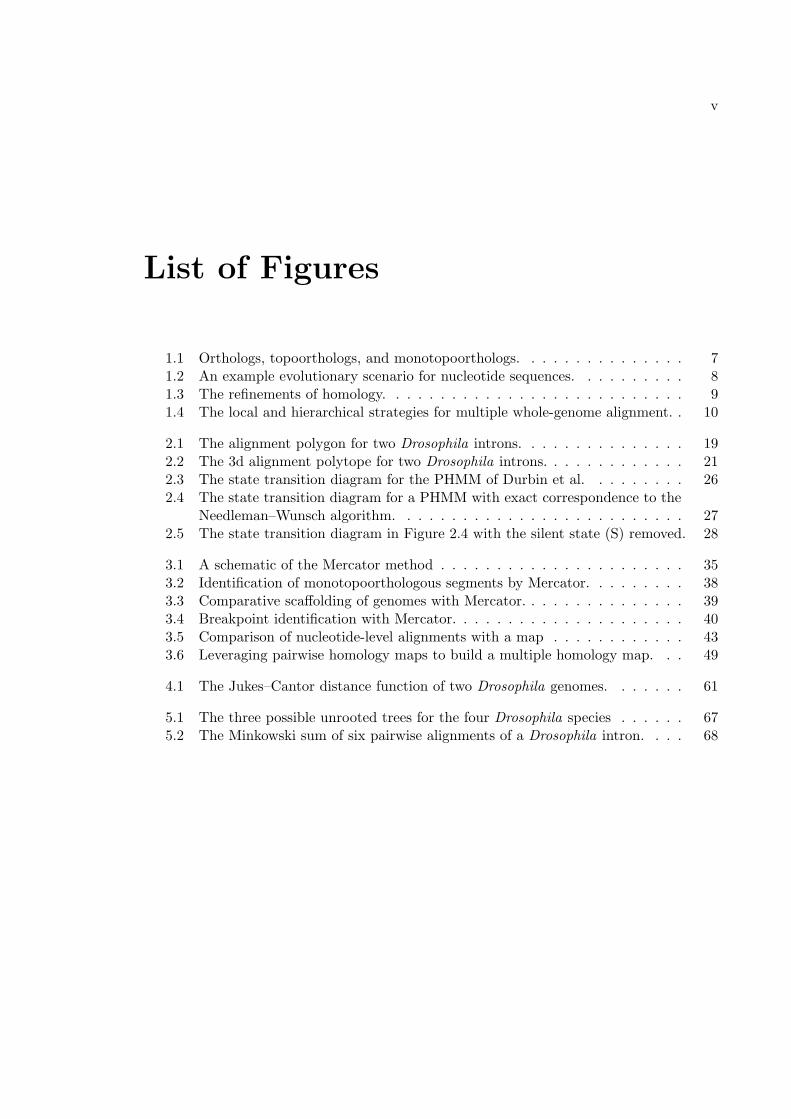
List of Figures

1.1 Orthologs, topoorthologs, and monotopoorthologs. . . . . . . . . . . . . . . 71.2 An example evolutionary scenario for nucleotide sequences. . . . . . . . . . 81.3 The refinements of homology. . . . . . . . . . . . . . . . . . . . . . . . . . . 91.4 The local and hierarchical strategies for multiple whole-genome alignment. . 10

2.1 The alignment polygon for two Drosophila introns. . . . . . . . . . . . . . . 192.2 The 3d alignment polytope for two Drosophila introns. . . . . . . . . . . . . 212.3 The state transition diagram for the PHMM of Durbin et al. . . . . . . . . 262.4 The state transition diagram for a PHMM with exact correspondence to the

Needleman–Wunsch algorithm. . . . . . . . . . . . . . . . . . . . . . . . . . 272.5 The state transition diagram in Figure 2.4 with the silent state (S) removed. 28

3.1 A schematic of the Mercator method . . . . . . . . . . . . . . . . . . . . . . 353.2 Identification of monotopoorthologous segments by Mercator. . . . . . . . . 383.3 Comparative scaffolding of genomes with Mercator. . . . . . . . . . . . . . . 393.4 Breakpoint identification with Mercator. . . . . . . . . . . . . . . . . . . . . 403.5 Comparison of nucleotide-level alignments with a map . . . . . . . . . . . . 433.6 Leveraging pairwise homology maps to build a multiple homology map. . . 49

4.1 The Jukes–Cantor distance function of two Drosophila genomes. . . . . . . 61

5.1 The three possible unrooted trees for the four Drosophila species . . . . . . 675.2 The Minkowski sum of six pairwise alignments of a Drosophila intron. . . . 68

vi

List of Tables

1.1 A comparison of two whole-genome alignment strategies. . . . . . . . . . . . 14

2.1 The 8,362 optimal alignments for two Drosophila introns. . . . . . . . . . . 182.2 Three substitution matrices for parametric alignment. . . . . . . . . . . . . 202.3 Face numbers of the alignment polytopes for two Drosophila introns. . . . . 23

3.1 Agreement of pairwise alignments with Mercator pairwise maps . . . . . . . 443.2 Agreement of pairwise alignments with Mercator multiple map . . . . . . . 453.3 Results of the comparative scaffolding of human, mouse, and rat . . . . . . 46

4.1 Observed running times for the computation of alignment polytopes. . . . . 544.2 Numbers of vertices and facets for Drosophila alignment polytopes. . . . . . 554.3 Parametric analysis of cis-regulatory element conservation. . . . . . . . . . . 59

5.1 The ten most probable sets of optimal pairwise alignments. . . . . . . . . . 69

A.1 Web sites of programs for the alignment of multiple whole genomes. . . . . 96A.2 Web sites providing whole genome sequences. . . . . . . . . . . . . . . . . . 96A.3 File formats used by Mercator and MAVID. . . . . . . . . . . . . . . . . . . 96

vii

Acknowledgments

I give my utmost thanks to my adviser, Lior Pachter, who has challenged me to

achieve great things and supported me at every step of the way. As I can’t imagine having

chosen a better adviser, I thank my good friend Philip Sternberg for originally suggesting

that I take a course from Lior in my first year.

Parts of this work would never have been possible without my fantastic coauthors:

Peter Huggins, Kevin Woods, Bernd Sturmfels, and Lior Pachter. In addition to his con-

tributions as a collaborator, I thank Bernd Sturmfels for his great teachings and support of

my upcoming career.

For the great fun that kept me going through my graduate school years, I thank

all of my Bay Area friends. In particular, I thank my El Cerrito housemates: Rahul Thakar,

for his snarky and thoughtful remarks, Hayley Lam, for her delicious meals and uplifting

laughter, Ryan Tang, for the amazing soup, and Arun Chawan, for his company during the

World Cup games. For helping me to take a break every once and a while during my last

year, I am grateful to my friends Jason Pittenger and Caryn Shield.

Last, but not least, I thank my family. Without the constant support of my

mother, Kay, my father, Jim, and my brother, Jamie, I could never have made it this far.

1

Chapter 1

Introduction

With the genome sequences of numerous species at hand, we have the opportunity

to discover how evolution has acted at each and every nucleotide in our genome. To this

end, we must identify sets of nucleotides that have descended from a common ancestral

nucleotide. The problem of identifying evolutionary related nucleotides is that of sequence

alignment, which is central to the field of comparative genomics. When the sequences under

consideration are entire genomes, we have the problem of multiple whole-genome alignment.

In this introduction, a series of definitions for homology and its subrelations between single

nucleotides will be stated. Within the framework of these definitions, we will describe how

alignments specify such relations and review the current methods available for the alignment

of multiple large genomes. We then describe a subset of tools that make biological inferences

from multiple whole genome alignments. The majority of the material in this chapter comes

from the review article [36].

1.1 Comparative genomics

Comparative genomics [76, 54] is the use of molecular evolution as a tool in the

investigation of biological processes. Nucleotide sequences common to the genomes of several

diverged species are indicative of shared biology, while differences in genomic sequence and

structure may shed light on what makes species distinct. The identification of genomic

elements that have been conserved over time allows biologists to focus their experiments

on those parts of the genome that are fundamental to much of life. Thus, methods for

the comparison of genomes and prediction of elements constrained by evolution have been

2

actively researched as of late.

Often implicit in the discussion of conserved or common sequences is the concept

of homology. Homology, famously defined by Richard Owen as “the same organ in different

animals under every variety of form and function,” is accepted by most as common ancestry

[51]. This important concept relies on the identification of evolutionary characters, distinct

entities between which we may assign ancestral relationships. First used in reference to

morphological characters, such as eye color or petal number, homology has since been used

in reference to characters of all levels, from the molecular to the behavioral. Our recently

acquired ability to identify single nucleotides in the genomes of different species allows us

to specify homology at the smallest scale. The definition and identification of homology at

this scale is the focus of our review.

The prediction of homology between nucleotides relies on the fact that genomic

positions derived from a common ancestral position are more likely to have the same state:

one of A, C, G, or T. With only four states and, often, billions of genomic positions, we

cannot simply use the coincidence of bases at two positions as a basis for assigning homology.

Therefore, we must take advantage of context. Positions adjacent in an ancestral sequence

are likely to be adjacent in the extant sequences. Predicting homology between genomic

positions is thus the problem of identifying colinear segments having statistically significant

numbers of similar states. Because we are faced with analyzing multiple large genomes, this

task requires expertise from the fields of computer science, statistics, and mathematics. In

these fields, the task of identifying related positions in sequences is the problem of alignment.

Although alignment is based on the identification of similar sequences, similarity

is not equivalent to homology. Similar, but unrelated sequences may arise simply by chance,

or through convergent evolution. On the other hand, sequences may be homologous but

not share a single similar character. In general, alignments may be used to specify relation-

ships other than common ancestry, such as structural or functional similarities. Although

identifying other classes of similarities between sequences is important, such similarities are

best understood in the light of evolution. Therefore, we focus on the problem of evolution-

ary alignment, which aims to identify only homologous relationships between nucleotide

positions.

3

1.2 Nucleotide homology

When Watson and Crick noted that “the specific pairing we have postulated imme-

diately suggests a possible copying mechanism for the genetic material,” [111] they alluded

to the most fundamental level of ancestry. Although homology is used at many levels of

biology, it is most directly defined with respect to nucleotide sequences. It is not clear from

the literature that people have agreed on a precise definition of nucleotide homology. Given

that the molecular mechanisms of nucleic acid replication are well known, it is important

from an evolutionary theory standpoint that such definitions are established. Moreover,

if we are to design and compare methods that predict homology between nucleotides, we

must have concrete definitions of the problem at hand. These definitions, however, must be

based on biology and not on what is possibly identified by our methods. Adhering to this

ideology, we propose definitions for nucleotide homology.

At the nucleic acid level, an evolutionary character is a position in single or double-

stranded DNA or RNA. The copying mechanism for nucleic acids is a single-stranded phe-

nomenon, and therefore we begin our definitions with the single-stranded case. For a single-

stranded nucleic acid, a character x has two properties: its position, traditionally counted

from the 5’ end of the polymer, and its state, which is one of A, C, G, T, or U. A single-

stranded character x is a copy of a character y if x was initially base-paired with y at the

time when x was added to its polymer. In such cases, the process by which x is added

to its polymer is called template-dependent synthesis [13] and y is called the template for

x. Positions added to a polymer without a template (e.g., adenines added during poly(A)

extension of mRNAs) have no such relationships.

In the double-stranded case, a character x comprises two single-stranded charac-

ters, x+ and x−, which are base-paired. Like a single-stranded character, double-stranded

characters have a position (usually given as the position of x+), and a state. The state of a

double-stranded character depends on a third property, its orientation, which we indicate

by one of + or −. If x has an orientation of +, then its state is that of x+ (the character on

the forward strand), otherwise it is that of x− (the character on the reverse strand). One

of x+ or x− is usually a copy of the other, with exceptions occurring due to mechanisms

such as replication slippage [13]. Given a double-stranded character x and a single-stranded

character y, x is a copy of y, if one of x+ or x− is a copy of y. Conversely, y is copy of x if

y is a copy of x+ or x−. If both x and y are double-stranded, then x is a copy of y if one

4

of x+ or x− is a copy of y+ or y−.

We now address mutation, the second major mechanism in molecular evolution.

Because characters are positions, point mutations of single-stranded characters do not

change their copy relationships. For example, if x is a copy of y and a point mutation

changes the state of x from A to G, then x is still a copy of y. However, in double-stranded

DNA, repair mechanisms may use the template of an opposite strand or a homologous re-

gion to replace damaged positions. Whenever a position is excised and restored using a

template, a new copy relationship is established.

Having discussed the concepts of copying and mutation, we now define homology.

For both types of characters, we say that x is derived from y if there is an ordered set

of characters, x1, x2, . . . , xT , such that y = x1, x = xT , and xt+1 is a copy of xt. The

ordered set may include both single-stranded and double-stranded characters. A character

x is homologous to a character y if there exists (or existed) a character z such that both x

and y are derived from z.

1.3 Refinements of nucleotide homology

1.3.1 Primary refinements

Molecular homology has traditionally been divided into three subrelations: or-

thology, paralogy, and xenology [44]. Although these refinements have distinct biological

implications [63], it is difficult to state unambiguous definitions for them in terms of biolog-

ical mechanisms. Nevertheless, the distinctions made by orthology, paralogy, and xenology

are important and the alignment methods we discuss distinguish between them. We there-

fore describe how orthology, paralogy, and xenology are applied at the nucleotide level.

Homology is first refined by the relation of xenology. Consider two homologous

nucleic acid positions, x and y, whose last common ancestor is z. These characters are

xenologous if at least one is derived from a position w, derived from z, that was horizon-

tally transferred. That is, the species to which w belonged changed during w’s existence

(excluding changes from a parent to a child species).

If x and y are not xenologous, then they are either orthologous or paralogous,

depending on the events undergone by z and its copies. Replication of genomic nucleic acids

is a regular occurrence in cells, with copies of the same genetic material normally separating

5

from each other during cell division. When cell divisions (either through mitosis, meiosis,

or binary fission) do not separate genomic copies, paralogous relationships are established.

To make this more precise, suppose that z is copied, resulting in two characters z1 and z2

in the same cell, where x is derived from z1 and y is derived from z2. If z1 and z2 are not

subsequently separated by cytokinesis, then x and y are paralogous. Otherwise, x and y are

orthologous.

1.3.2 Secondary refinements

When describing relationships between genomic characters, the notion of context is

critical. As far as the fundamental terms of orthology and paralogy are concerned, genomes

could be viewed as “bags of genes,” i.e., a set of genomic elements without an ordering

or grouping on chromosomes. Therefore, when we take into consideration the context of

genomic elements, more precise terms are required for describing the relationships between

them, as we illustrate with the following example. Suppose that genesX and Y are orthologs

and are the only members of a certain gene family in two genomes. If a mRNA of Y

subsequently becomes retrotransposed elsewhere in the genome, resulting in a gene Y ′

(possibly non-functional), then X will be orthologous to both Y and Y ′. Orthology does not

distinguish between the two copies of Y , even though they are quite different contextually

and, likely, functionally.

In an attempt to take context into account, researchers have often used the word

“synteny” in describing genomic segments that have been left untouched by genomic re-

arrangements during evolution in several lineages. Unfortunately, this term often used

incorrectly or ambiguously [84]. By itself, the word “synteny” neither implies homology

nor colinearity of related elements. Therefore, we advocate discontinuing the use of such

widespread phrases as “synteny map” and “synteny block” in favor of more precise terms.

Although of similar etymology to “synteny”, we favor use of the word “colinear,” as fa-

mously used by [113], in combination with evolutionary terms to describe relationships

between genomic characters.

We introduce a series of definitions that allow us to describe both evolutionary and

contextual relationships. The first two definitions distinguish between genomic duplication

events and are the basis for the later concepts. In the following definitions, for some genetic

material A and a genome G, we use G+A and G−A to denote the result of the insertion

6

of A into G and the result of the removal of A from G, respectively.

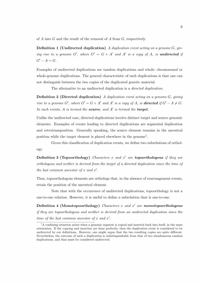
Definition 1 (Undirected duplication) A duplication event acting on a genome G, giv-

ing rise to a genome G′, where G′ = G + A′ and A′ is a copy of A, is undirected if

G′ −A = G.

Examples of undirected duplications are tandem duplications and whole- chromosomal or

whole-genome duplications. The general characteristic of such duplications is that one can

not distinguish between the two copies of the duplicated genetic material.

The alternative to an undirected duplication is a directed duplication.

Definition 2 (Directed duplication) A duplication event acting on a genome G, giving

rise to a genome G′, where G′ = G+A′ and A′ is a copy of A, is directed if G′ −A 6= G.

In such events, A is termed the source, and A′ is termed the target.

Unlike the undirected case, directed duplications involve distinct target and source genomic

elements. Examples of events leading to directed duplications are segmental duplication

and retrotransposition. Generally speaking, the source element remains in the ancestral

position while the target element is placed elsewhere in the genome1.

Given this classification of duplication events, we define two subrelations of orthol-

ogy.

Definition 3 (Topoorthology) Characters x and x′ are topoorthologous if they are

orthologous and neither is derived from the target of a directed duplication since the time of

the last common ancestor of x and x′.

Thus, topoorthologous elements are orthologs that, in the absence of rearrangement events,

retain the position of the ancestral element.

Note that with the occurrence of undirected duplications, topoorthology is not a

one-to-one relation. However, it is useful to define a subrelation that is one-to-one.

Definition 4 (Monotopoorthology) Characters x and x′ are monotopoorthologous

if they are topoorthologous and neither is derived from an undirected duplication since the

time of the last common ancestor of x and x′.1A confusing situation arises when a genomic segment is copied and inserted back into itself, in the same

orientation. If the copying and insertion are done perfectly, then the duplication event is considered to beundirected by our definitions. However, one might argue that the two resulting copies are quite different.Nevertheless, the outcome of such a duplication is indistinguishable from that of two simultaneous tandemduplications, and thus must be considered undirected.

7

XA YA1 YA2 ZA XB YB XB2ZB

X Y Z

XA YA ZA XB YB ZBspeciation

undirectedduplication

directedduplication

YBYA2YA1

Y

A

B

XA XB XB2

X

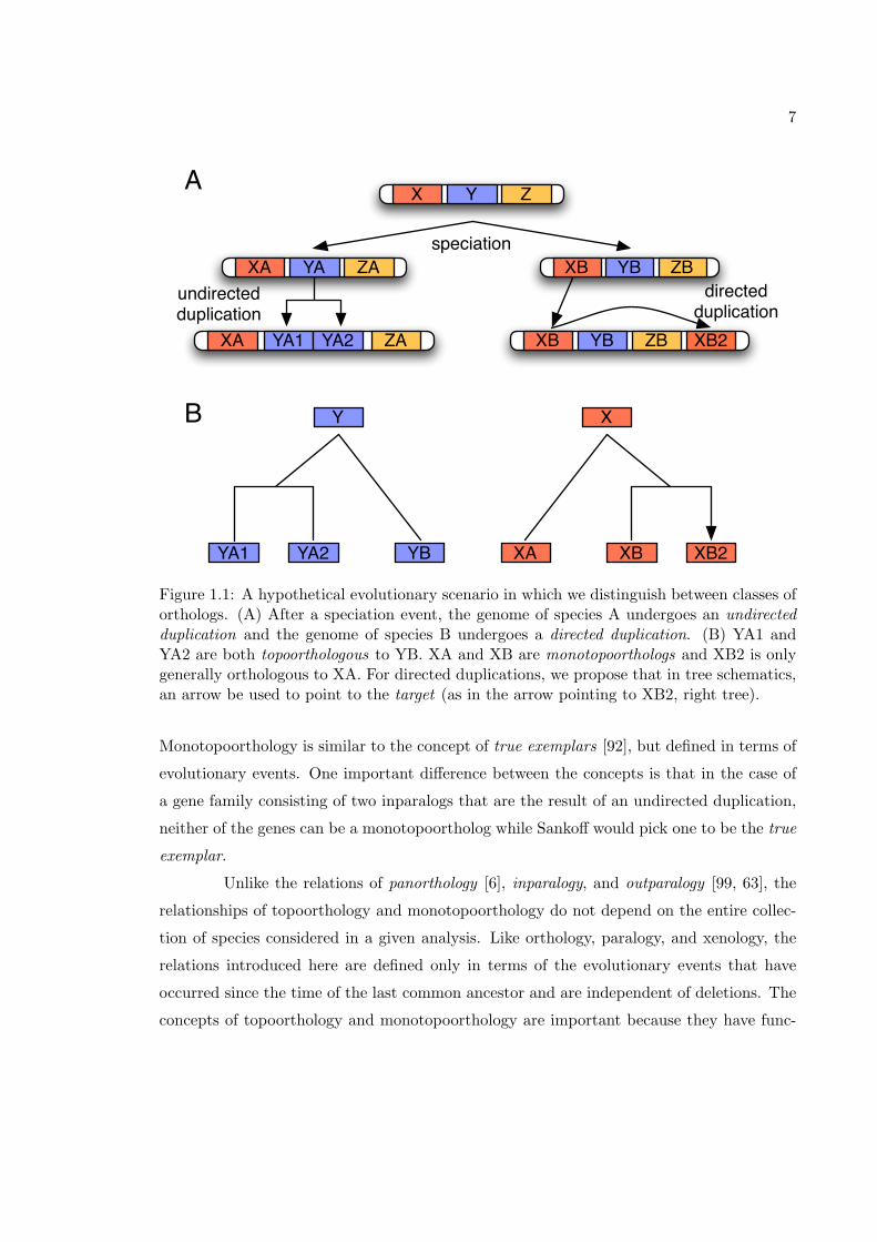
Figure 1.1: A hypothetical evolutionary scenario in which we distinguish between classes oforthologs. (A) After a speciation event, the genome of species A undergoes an undirectedduplication and the genome of species B undergoes a directed duplication. (B) YA1 andYA2 are both topoorthologous to YB. XA and XB are monotopoorthologs and XB2 is onlygenerally orthologous to XA. For directed duplications, we propose that in tree schematics,an arrow be used to point to the target (as in the arrow pointing to XB2, right tree).

Monotopoorthology is similar to the concept of true exemplars [92], but defined in terms of

evolutionary events. One important difference between the concepts is that in the case of

a gene family consisting of two inparalogs that are the result of an undirected duplication,

neither of the genes can be a monotopoortholog while Sankoff would pick one to be the true

exemplar.

Unlike the relations of panorthology [6], inparalogy, and outparalogy [99, 63], the

relationships of topoorthology and monotopoorthology do not depend on the entire collec-

tion of species considered in a given analysis. Like orthology, paralogy, and xenology, the

relations introduced here are defined only in terms of the evolutionary events that have

occurred since the time of the last common ancestor and are independent of deletions. The

concepts of topoorthology and monotopoorthology are important because they have func-

8

tional implications. Orthologous genes are likely to have more similar functions if they

are topoorthologs because they have similar genomic contexts [81]. Monotopoorthologs are

even more likely to have identical functions because there is less opportunity for subfunc-

tionalization to occur when only one gene remains in the ancestral position.

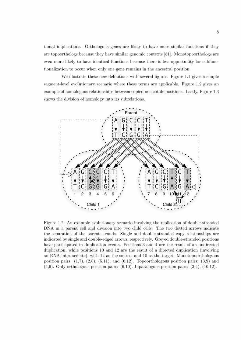
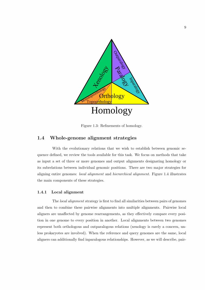
We illustrate these new definitions with several figures. Figure 1.1 gives a simple

segment-level evolutionary scenario where these terms are applicable. Figure 1.2 gives an

example of homologous relationships between copied nucleotide positions. Lastly, Figure 1.3

shows the division of homology into its subrelations.

A

T

G

C

C

G

C

G

C

G

T

A

A

T

G

C

C

G

C

G

T

A

A

T

G

C

C

G

C

G

T

A

U

T

A1 2 3 4 5 6 7 8 9 10 11 12

Parent

Child 1 Child 2

Figure 1.2: An example evolutionary scenario involving the replication of double-strandedDNA in a parent cell and division into two child cells. The two dotted arrows indicatethe separation of the parent strands. Single and double-stranded copy relationships areindicated by single and double-edged arrows, respectively. Greyed double-stranded positionshave participated in duplication events. Positions 3 and 4 are the result of an undirectedduplication, while positions 10 and 12 are the result of a directed duplication (involvingan RNA intermediate), with 12 as the source, and 10 as the target. Monotopoorthologousposition pairs: (1,7), (2,8), (5,11), and (6,12). Topoorthologous position pairs: (3,9) and(4,9). Only orthologous position pairs: (6,10). Inparalogous position pairs: (3,4), (10,12).

9

Paralogy

Xeno

logy

TopoorthologyMonotopoorthologyOutparalogy

Inparalogy

Orthology

HomologyFigure 1.3: Refinements of homology.

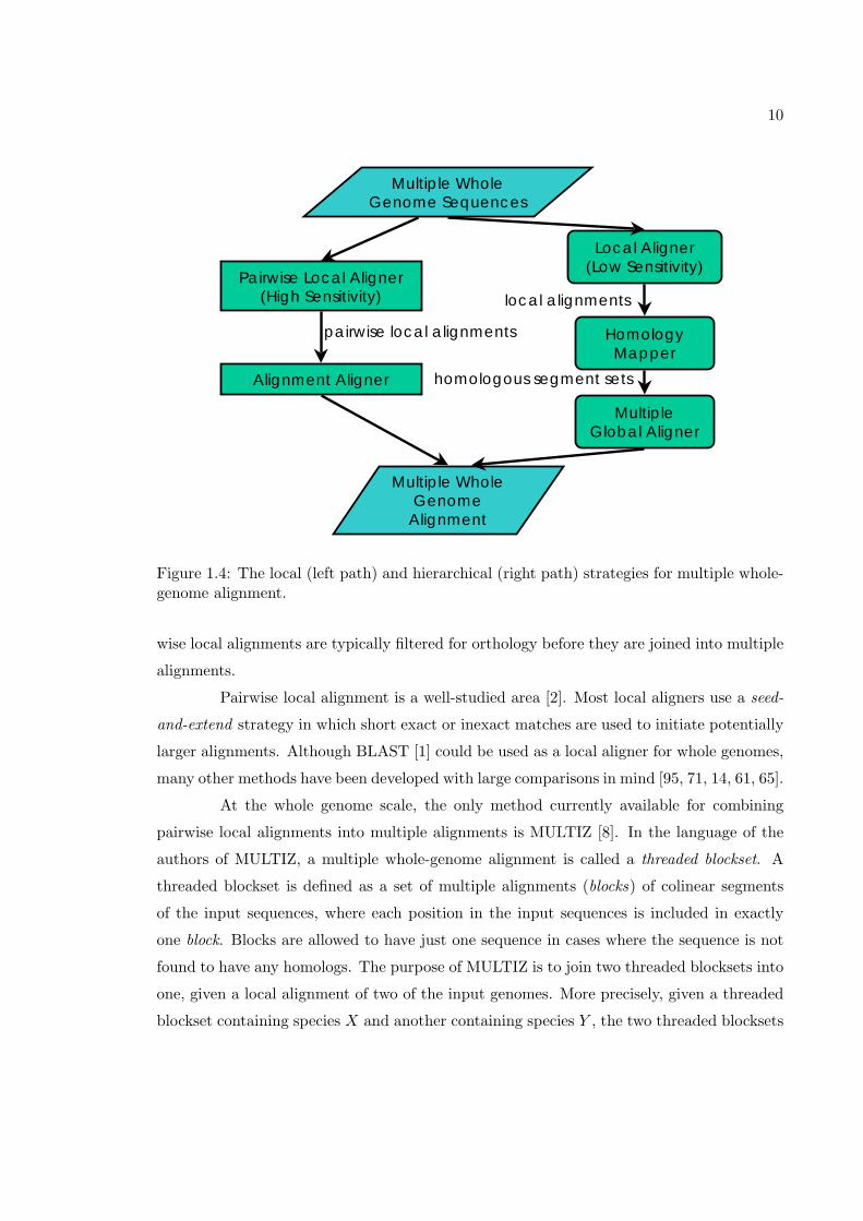
1.4 Whole-genome alignment strategies

With the evolutionary relations that we wish to establish between genomic se-

quence defined, we review the tools available for this task. We focus on methods that take

as input a set of three or more genomes and output alignments designating homology or

its subrelations between individual genomic positions. There are two major strategies for

aligning entire genomes: local alignment and hierarchical alignment. Figure 1.4 illustrates

the main components of these strategies.

1.4.1 Local alignment

The local alignment strategy is first to find all similarities between pairs of genomes

and then to combine these pairwise alignments into multiple alignments. Pairwise local

aligners are unaffected by genome rearrangements, as they effectively compare every posi-

tion in one genome to every position in another. Local alignments between two genomes

represent both orthologous and outparalogous relations (xenology is rarely a concern, un-

less prokaryotes are involved). When the reference and query genomes are the same, local

aligners can additionally find inparalogous relationships. However, as we will describe, pair-

10

Multiple Whole Genome Sequences

Pairwise Local Aligner (High Sensitivity)

Local Aligner(Low Sensitivity)

Homology Mapper

Multiple Global Aligner

Alignment Aligner

Multiple Whole Genome

Alignment

pairwise local alignments

homologous segment sets

local alignments

Figure 1.4: The local (left path) and hierarchical (right path) strategies for multiple whole-genome alignment.

wise local alignments are typically filtered for orthology before they are joined into multiple

alignments.

Pairwise local alignment is a well-studied area [2]. Most local aligners use a seed-

and-extend strategy in which short exact or inexact matches are used to initiate potentially

larger alignments. Although BLAST [1] could be used as a local aligner for whole genomes,

many other methods have been developed with large comparisons in mind [95, 71, 14, 61, 65].

At the whole genome scale, the only method currently available for combining

pairwise local alignments into multiple alignments is MULTIZ [8]. In the language of the

authors of MULTIZ, a multiple whole-genome alignment is called a threaded blockset. A

threaded blockset is defined as a set of multiple alignments (blocks) of colinear segments

of the input sequences, where each position in the input sequences is included in exactly

one block. Blocks are allowed to have just one sequence in cases where the sequence is not

found to have any homologs. The purpose of MULTIZ is to join two threaded blocksets into

one, given a local alignment of two of the input genomes. More precisely, given a threaded

blockset containing species X and another containing species Y , the two threaded blocksets

11

are joined by a pairwise alignment between X and Y .

The UCSC Genome Browser [59] currently provides MULTIZ genome alignments

for vertebrates, insects, and yeast. For each of these alignments, the pairwise BLASTZ [95]

alignments given to MULTIZ as input are first filtered with a “best-in-genome” criterion

[62]. Given a pairwise alignment between a reference and a query genome, this filter keeps

only the best alignment for each position in the reference genome. The filtered alignments

are assumed to specify only orthologous relationships. Unless applied in a reciprocal man-

ner, these filters give many-to-one orthology relationships between a reference and a query

genome. Although not capturing all orthologous relationships, the resulting reference-based

multiple alignments have the convenient property that every column has at most one posi-

tion from each genome.

1.4.2 Hierarchical alignment

A second strategy for multiple whole genome alignment combines homology map-

ping with efficient global alignment. Homology maps identify sets of large colinear homol-

ogous segments between multiple genomes, and are typically designed to find only mono-

topoorthologous relationships. For example, a homology map might specify that intervals

38,400,000-38,529,874 of human chromosome 17, 101,551,137-101,659,587 of mouse chro-

mosome 11, and 90,483,833-90,585,675 of rat chromosome 10 (all intervals on the forward

strand) contain monotopoorthologous and colinear positions (these intervals contain the

BRCA1 gene). Genomic global alignment programs, which require colinearity, are run on

segments (such as those just mentioned as an example) specified by a homology map to

produce nucleotide level alignments.

Methods for homology mapping typically take as input sets of pairwise local align-

ments and output sets of genomic segments containing significant numbers of local align-

ments that occur in the same order and orientation. After the sequencing of the third

large genome, that of the rat [45], several methods were developed for the construction of

multiple genome homology maps. GRIMM-Synteny [10], combines the output of a sensitive

local aligner, such as PatternHunter [71], between all pairs of k genomes to first produce

k-way anchors. Nearby and consistent k-way anchors are joined to produce a k-way orthol-

ogy map. Mauve [30], a related method that uses multi-MUM (multiple maximal unique

match) local alignments [31] to construct orthology maps between multiple closely related

12

species, has been demonstrated to create maps between the human, mouse, and rat. Both

Mauve and GRIMM-Synteny output one-to-one maps between genomes, which are indica-

tive of monotopoorthology. PARAGON [94], another similar method that uses BLASTZ

alignments as input, has been used to create orthology maps between more distant species.

Another method used to align the human, mouse, and rat genomes [16] uses a

progressive extension of a pairwise strategy engineered for aligning human to mouse [28].

Using the BLAT [61] local aligner, a mouse-rat orthology map was first constructed. The

orthologous segments were aligned using the LAGAN [15] global aligner, mapped to the

human genome using BLAT, and finally put into a multiple alignment using MLAGAN.

The resulting maps represented all orthology relationships, although most genomic segments

were found to be monotopoorthologous. A final method used for human, mouse, and rat

orthology mapping used BAC end sequence comparisons as a basis for orthologous anchors

[115].

In Chapter 3, a monotopoorthology mapping method called Mercator will be de-

scribed. Here we provide a brief overview of Mercator so that it may be compared with the

other methods described in this section. Mercator takes as input a set of non-overlapping

landmarks in each genome and pairwise similarity scores between all landmarks. A graph is

constructed with landmarks as vertices and hits between them as edges. Within this graph,

Mercator identifies high-scoring cliques, i.e., sets of landmarks (in this graph, containing at

most one landmark from each genome) where there is a significant hit between each pair.

For example, if exons are used as landmarks, then the first exons of the human, mouse, and

rat SHH gene would be identified as a high-scoring clique. Such cliques indicate orthologous

relationships. Starting with the largest cliques (those in which we are most confident), ad-

jacent and consistent cliques (such as those formed from each exon of SHH ) are joined into

runs that represent orthologous segments. Edges not consistent with previously identified

runs are discarded and smaller cliques are discovered in the graph and incorporated into

runs. The algorithm iterates until cliques involving all possible combinations of genomes

have been considered. Thus, unlike most other monotopoorthology mapping methods, Mer-

cator produces maps comprising sets of segments that may be specific to any subset of the

input genomes.

Once colinear homologous segments have been identified, multiple global align-

ment programs are used to assign homologous relationships between individual positions.

Global aligners create a one-to-one mapping between the positions of two sequences. Thus,

13

in the absence of recent tandem duplications, multiple global aligners will determine the

monotopoorthologous positions in a a set of colinear monotopoorthologous segments. The

only methods that have been run on whole large genomes thus far are MAVID [12], and

MLAGAN [15]. Both rely on global chaining of short matches between pairs of sequences.

A chain is simply an ordered set of locally aligned segments with the property that the

coordinates of the segments of the ith local alignment in the chain are less than those of

the segments of the jth local alignment, when i < j. To create a multiple alignment, both

methods use a progressive strategy. MAVID and MLAGAN differ in their identification

of local alignment anchors (exact vs. inexact) and the methods by which alignments are

aligned at internal nodes of the phylogenetic tree (ancestral reconstruction vs. via sum-of-

pairs). Other multiple genomic global aligners that have not been run on whole genomes

but are comparable are given in [14, 8, 114].

1.4.3 Comparison of alignment strategies

Currently, all local and hierarchical multiple alignment methods focus on orthol-

ogy. They either identify many-to-many, many-to-one, or one-to-one (monotopoortholo-

gous) relationships. Hierarchical methods begin by using local alignments, but typically do

not use local methods with their most sensitive parameter settings. This results in much

faster running times at the expense of missing short and significantly diverged ortholo-

gous sequence. Although less sensitive at the genome-wide scale, the hierarchical strategy

can afford to use more sensitive methods at a smaller scale, within the sets of orthologous

segments identified by the map.

An important difference between the two strategies is the treatment of genomic

segments that have been inserted or deleted during evolution. Given a set of orthologous

segments, global aligners will gap all positions that are not found to have orthologous rela-

tions. With recent insertions of mobile elements, these gaps can often be very large. Local

alignments, on the other hand, are not extended through longer insertions and deletions.

Segments that are not part of any local alignment may be interpreted in two ways. One

way is to treat orthologous relationships to such segments as missing data. A second in-

terpretation is that segments not part of any alignment are implicitly gapped, i.e., they

are believed to have been inserted or deleted. The choice of alignment strategy and the

treatment of gaps are issues that researchers must be aware of when using multiple whole

14

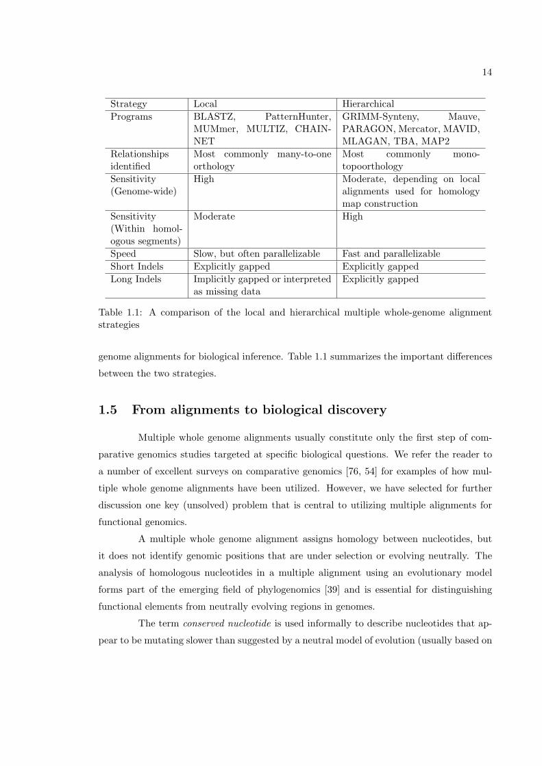
Strategy Local HierarchicalPrograms BLASTZ, PatternHunter,

MUMmer, MULTIZ, CHAIN-NET

GRIMM-Synteny, Mauve,PARAGON, Mercator, MAVID,MLAGAN, TBA, MAP2

Relationshipsidentified

Most commonly many-to-oneorthology

Most commonly mono-topoorthology

Sensitivity(Genome-wide)

High Moderate, depending on localalignments used for homologymap construction

Sensitivity(Within homol-ogous segments)

Moderate High

Speed Slow, but often parallelizable Fast and parallelizableShort Indels Explicitly gapped Explicitly gappedLong Indels Implicitly gapped or interpreted

as missing dataExplicitly gapped

Table 1.1: A comparison of the local and hierarchical multiple whole-genome alignmentstrategies

genome alignments for biological inference. Table 1.1 summarizes the important differences

between the two strategies.

1.5 From alignments to biological discovery

Multiple whole genome alignments usually constitute only the first step of com-

parative genomics studies targeted at specific biological questions. We refer the reader to

a number of excellent surveys on comparative genomics [76, 54] for examples of how mul-

tiple whole genome alignments have been utilized. However, we have selected for further

discussion one key (unsolved) problem that is central to utilizing multiple alignments for

functional genomics.

A multiple whole genome alignment assigns homology between nucleotides, but

it does not identify genomic positions that are under selection or evolving neutrally. The

analysis of homologous nucleotides in a multiple alignment using an evolutionary model

forms part of the emerging field of phylogenomics [39] and is essential for distinguishing

functional elements from neutrally evolving regions in genomes.

The term conserved nucleotide is used informally to describe nucleotides that ap-

pear to be mutating slower than suggested by a neutral model of evolution (usually based on

15

a continuous time Markov model for point mutation [41]). Groups of conserved nucleotides

are called conserved elements. To our knowledge, there is no precise definition of conserved

elements at this time. Software tools that have been developed for identifying conserved

nucleotides and elements include GERP [27], PhastCons [96], BinCons [72], and Shadower

[75]. Conserved elements can also be identified by examining insertions and deletions within

multiple alignments. This has been described in [70, 98]. In [36], there is a discussion of how

the choice of alignment affects the determination of conserved nucleotides, and estimation

of evolutionary model parameters.

The problem of identifying conservation within multiple alignments is inherently

a statistics problem, but one that requires further advances by biologists in experimentally

validating functional elements. Such advances are crucial for defining appropriate choices

of evolutionary models, and will subsequently inform computational biologists on the best

ways to predict new functional elements.

16

Chapter 2

Nucleotide-level alignment: models

and polytopes

The majority of methods for the alignment of nucleotide sequences include, as a

component, the classic Needleman–Wunsch global alignment algorithm [80]. In this chapter,

we analyze this algorithm from both parametric and statistical points of view. Parametric

alignment, which determines the dependencies of optimal alignments on parameter values, is

described in terms of alignment polytopes. A statistical model with a direct correspondence

to the Needleman–Wunsch algorithm is also presented. The parametric alignment aspects

of this chapter come from the paper [34].

2.1 Parametric alignment

2.1.1 Motivation

Needleman–Wunsch pairwise sequence alignment is known to be sensitive to pa-

rameter choices. To illustrate the problem, consider the 8th intron of the Drosophila

melanogaster CG9935-RA gene (as annotated by FlyBase [37]) located on chr4:660,462-

660,522 (April 2004 BDGP release 4). This intron, which is 61 base pairs long, has

a 60 base pair ortholog in Drosophila pseudoobscura. The ortholog is located at Con-

tig8094 Contig5509:4,876-4,935 in the August 2003, freeze 1 assembly, as produced by the

Baylor Genome Sequencing Center.Using the basic 3-parameter scoring scheme (match M , mismatch X and space

17

penalty S), these two orthologous introns have the following optimal alignment when theparameters are set to M = 5, X = −5 and S = −5:

mel GTAAGTTTGTTTAT-ATTTTTTTTTTTTTGAAGTGA-CAAATAGC-A-CTTATAAATATACTTAGpse GTTCGTTAACACATGAAATTCCATCGCCTGAT-TGTTCA-CTATCTAACTAACGAAT-T--TTAG

** *** ** * ** * *** ** ** ** * * ** * *** * ****However, if we change the parameters to M = 5, X = −6 and S = −4, then the followingalignment is optimal:

mel GTAAGTT------TGTTTATATTTTTTTT--T--TT-TTGAAGTGA-CAAATAGCACTTATA--Apse GTTCGTTAACACATG-A-A-ATTCCATCGCCTGATTGTT-CACT-ATC---TA--AC-TA-ACGA

** *** ** * *** * * ** ** * * * * ** ** ** * *

mel ATATACTTAGpse AT-T--TTAG

** * ****

Note that a relatively small change in the parameters produces a very different alignment

of the introns. This problem is exacerbated with more complex scoring schemes, and is

a central issue with whole-genome alignments produced by programs such as MAVID [11]

or BLASTZ/MULTIZ [95]. Indeed, although whole genome alignment systems use many

heuristics for rapidly identifying alignable regions and subsequently aligning them, they

all rely on the Needleman–Wunsch algorithm at some level. Dependence on parameters

becomes an even more crucial issue in the multiple alignment of more than two sequences.

Parametric alignment was introduced by Waterman, Eggert and Lander [109] and

further developed by Gusfield et al. [48, 49] and Fernandez-Baca et al. [42] as an approach

for overcoming the difficulties in selecting parameters for Needleman–Wunsch alignment.

See [43] for a review and [82, 83] for an algebraic perspective. Parametric alignment amounts

to partitioning the space of parameters into regions. Parameters in the same region lead to

the same optimal alignments. Enumerating all regions is a non-trivial problem of compu-

tational geometry. The following sections present our approach to solving this problem. In

Chapter 4 we solve this problem on a whole genome scale for up to five free parameters.

2.1.2 Alignment summaries

We present an approach to parametric alignment that rests on the idea that the

score of an alignment is specified by a short list of numbers derived from the alignment. For

instance, given the standard 3-parameter scoring scheme, we summarize each alignment by

the number m of matches, the number x of mismatches, and the number s of spaces in the

18

alignment. The triple (m,x, s) is called the alignment summary. As an example consider the

pair of orthologous Drosophila introns given in Section 2.1.1. The first (shorter) alignment

has the alignment summary (33, 23, 9) while the second (longer) alignment has the alignment

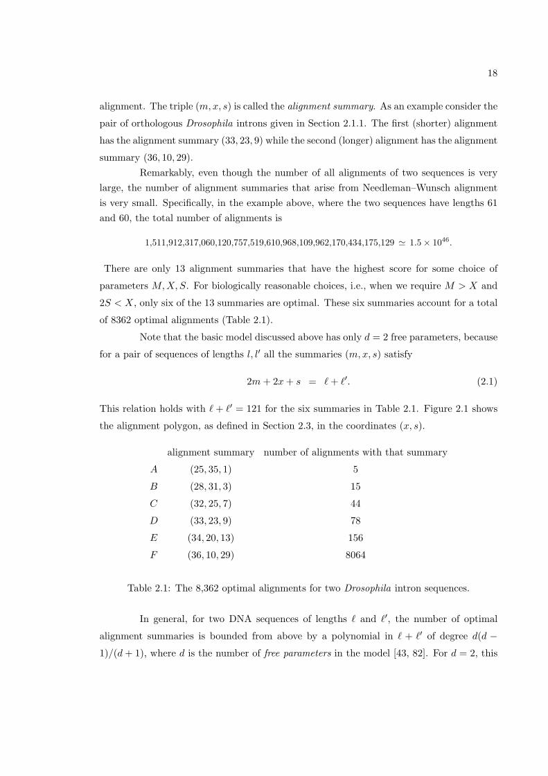
summary (36, 10, 29).Remarkably, even though the number of all alignments of two sequences is very

large, the number of alignment summaries that arise from Needleman–Wunsch alignmentis very small. Specifically, in the example above, where the two sequences have lengths 61and 60, the total number of alignments is

1,511,912,317,060,120,757,519,610,968,109,962,170,434,175,129 ' 1.5× 1046.

There are only 13 alignment summaries that have the highest score for some choice of

parameters M,X,S. For biologically reasonable choices, i.e., when we require M > X and

2S < X, only six of the 13 summaries are optimal. These six summaries account for a total

of 8362 optimal alignments (Table 2.1).

Note that the basic model discussed above has only d = 2 free parameters, because

for a pair of sequences of lengths l, l′ all the summaries (m,x, s) satisfy

2m+ 2x+ s = `+ `′. (2.1)

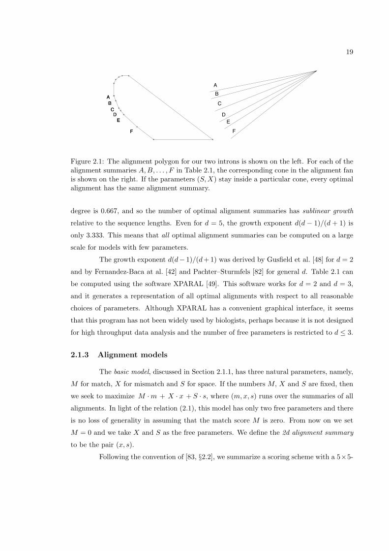
This relation holds with `+ `′ = 121 for the six summaries in Table 2.1. Figure 2.1 shows

the alignment polygon, as defined in Section 2.3, in the coordinates (x, s).

alignment summary number of alignments with that summary

A (25, 35, 1) 5

B (28, 31, 3) 15

C (32, 25, 7) 44

D (33, 23, 9) 78

E (34, 20, 13) 156

F (36, 10, 29) 8064

Table 2.1: The 8,362 optimal alignments for two Drosophila intron sequences.

In general, for two DNA sequences of lengths ` and `′, the number of optimal

alignment summaries is bounded from above by a polynomial in ` + `′ of degree d(d −1)/(d+ 1), where d is the number of free parameters in the model [43, 82]. For d = 2, this

19

C

AB

DE

F

CC

AABB

DDEE

FF

Figure 2.1: The alignment polygon for our two introns is shown on the left. For each of thealignment summaries A,B, . . . , F in Table 2.1, the corresponding cone in the alignment fanis shown on the right. If the parameters (S,X) stay inside a particular cone, every optimalalignment has the same alignment summary.

degree is 0.667, and so the number of optimal alignment summaries has sublinear growth

relative to the sequence lengths. Even for d = 5, the growth exponent d(d − 1)/(d + 1) is

only 3.333. This means that all optimal alignment summaries can be computed on a large

scale for models with few parameters.

The growth exponent d(d− 1)/(d+1) was derived by Gusfield et al. [48] for d = 2

and by Fernandez-Baca at al. [42] and Pachter–Sturmfels [82] for general d. Table 2.1 can

be computed using the software XPARAL [49]. This software works for d = 2 and d = 3,

and it generates a representation of all optimal alignments with respect to all reasonable

choices of parameters. Although XPARAL has a convenient graphical interface, it seems

that this program has not been widely used by biologists, perhaps because it is not designed

for high throughput data analysis and the number of free parameters is restricted to d ≤ 3.

2.1.3 Alignment models

The basic model, discussed in Section 2.1.1, has three natural parameters, namely,

M for match, X for mismatch and S for space. If the numbers M, X and S are fixed, then

we seek to maximize M ·m + X · x + S · s, where (m,x, s) runs over the summaries of all

alignments. In light of the relation (2.1), this model has only two free parameters and there

is no loss of generality in assuming that the match score M is zero. From now on we set

M = 0 and we take X and S as the free parameters. We define the 2d alignment summary

to be the pair (x, s).

Following the convention of [83, §2.2], we summarize a scoring scheme with a 5×5-

20

0 X X X S

X 0 X X S

X X 0 X S

X X X 0 S

S S S S

,

0 X Y X S

X 0 X Y S

Y X 0 X S

X Y X 0 S

S S S S

,

0 X Y Z S

X 0 Z Y S

Y Z 0 X S

Z Y X 0 S

S S S S

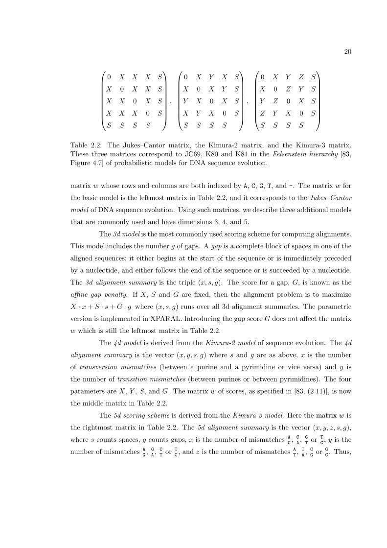
Table 2.2: The Jukes–Cantor matrix, the Kimura-2 matrix, and the Kimura-3 matrix.These three matrices correspond to JC69, K80 and K81 in the Felsenstein hierarchy [83,Figure 4.7] of probabilistic models for DNA sequence evolution.

matrix w whose rows and columns are both indexed by A, C, G, T, and -. The matrix w for

the basic model is the leftmost matrix in Table 2.2, and it corresponds to the Jukes–Cantor

model of DNA sequence evolution. Using such matrices, we describe three additional models

that are commonly used and have dimensions 3, 4, and 5.

The 3d model is the most commonly used scoring scheme for computing alignments.

This model includes the number g of gaps. A gap is a complete block of spaces in one of the

aligned sequences; it either begins at the start of the sequence or is immediately preceded

by a nucleotide, and either follows the end of the sequence or is succeeded by a nucleotide.

The 3d alignment summary is the triple (x, s, g). The score for a gap, G, is known as the

affine gap penalty. If X, S and G are fixed, then the alignment problem is to maximize

X · x+ S · s+G · g where (x, s, g) runs over all 3d alignment summaries. The parametric

version is implemented in XPARAL. Introducing the gap score G does not affect the matrix

w which is still the leftmost matrix in Table 2.2.

The 4d model is derived from the Kimura-2 model of sequence evolution. The 4d

alignment summary is the vector (x, y, s, g) where s and g are as above, x is the number

of transversion mismatches (between a purine and a pyrimidine or vice versa) and y is

the number of transition mismatches (between purines or between pyrimidines). The four

parameters are X, Y , S, and G. The matrix w of scores, as specified in [83, (2.11)], is now

the middle matrix in Table 2.2.

The 5d scoring scheme is derived from the Kimura-3 model. Here the matrix w is

the rightmost matrix in Table 2.2. The 5d alignment summary is the vector (x, y, z, s, g),

where s counts spaces, g counts gaps, x is the number of mismatches AC, CA, GT

or TG, y is the

number of mismatches AG, GA, CT

or TC, and z is the number of mismatches A

T, TA, CG

or GC. Thus,

21

g

s x

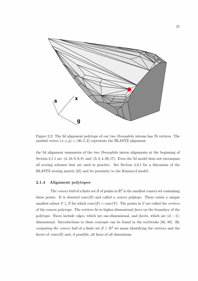
Figure 2.2: The 3d alignment polytope of our two Drosophila introns has 76 vertices. Themarked vertex (x, s, g) = (30, 5, 2) represents the BLASTZ alignment.

the 5d alignment summaries of the two Drosophila intron alignments at the beginning of

Section 2.1.1 are (4, 10, 9, 9, 8) and (3, 3, 4, 29, 17). Even the 5d model does not encompass

all scoring schemes that are used in practice. See Section 4.3.1 for a discussion of the

BLASTZ scoring matrix [25] and its proximity to the Kimura-2 model.

2.1.4 Alignment polytopes

The convex hull of a finite set S of points in Rd is the smallest convex set containing

these points. It is denoted conv(S) and called a convex polytope. There exists a unique

smallest subset V ⊆ S for which conv(S) = conv(V). The points in V are called the vertices

of the convex polytope. The vertices lie in higher-dimensional faces on the boundary of the

polytope. Faces include edges, which are one-dimensional, and facets, which are (d − 1)-

dimensional. Introductions to these concepts can be found in the textbooks [46, 88]. By

computing the convex hull of a finite set S ⊂ Rd we mean identifying the vertices and the

facets of conv(S) and, if possible, all faces of all dimensions.

22

Fix one of the four models discussed in Section 2.1.3. The alignment polytope of

two DNA sequences is the convex polytope conv(S) ⊂ Rd, where S is the set of alignment

summaries of all alignments of these two sequences. For instance, the 3d alignment polytope

of two DNA sequences is the convex polytope in R3 that is formed by taking the convex hull

of all alignment summaries (x, s, g). Figure 2.2 shows the 3d alignment polytope for the

two sequences in Section 2.1.1. Its projection onto the (x, s)-plane is the polygon depicted

in Figure 2.1.

It is a basic fact of convexity that the maximum of a linear function over a polytope

is attained at a vertex. Thus, an alignment of two DNA sequences is optimal if and only

if its summary is in the set V of vertices of the alignment polytope. The Needleman–

Wunsch algorithm efficiently solves the linear programming problem over this polytope.

For instance, for the 3d model with fixed parameters, the alignment problem is the linear

programming problem

Maximize X · x+ S · s+ g ·G subject to (x, s, g) ∈ V. (2.2)

For a numerical example consider the parameter values X = −200, S = −80 and G =−400, which represent an approximation of the BLASTZ scoring scheme (Section 3.1). Thesolution to (2.2) is attained at the vertex (x, s, g) = (30, 5, 2) which is the 3d summary ofthe following alignment of our two Drosophila introns

mel GTAAGTTTGTTTATATTTTTTTTTTTTTGAAGTGACAAATAGC--ACTTATAAATATACTTAGpse GTTCGTTAACACATGAAATTCCATCGCCTGATTGTTCACTATCTAACTAACGAAT---TTTAG

** *** ** ** * * ** * ** * *** * *** ****

The 3d summary of this alignment is the marked vertex in Figure 2.2.

As demonstrated by our discussion of alignment polytopes, convexity is the orga-

nizing principle that reveals the needles in the haystack. In our running example of two

Drosophila introns, the “haystack” consists of more than 1046 alignments, and the “nee-

dles” are the 8362 optimal alignments. Thus, parametric alignment of two DNA sequences

relative to some chosen scoring scheme means constructing the alignment polytope of the

two sequences.

2.1.5 Robustness cones

Suppose we are given a specific alignment of two DNA sequences. Then the ro-

bustness cone of that alignment is the set of all parameter vectors that have the following

23

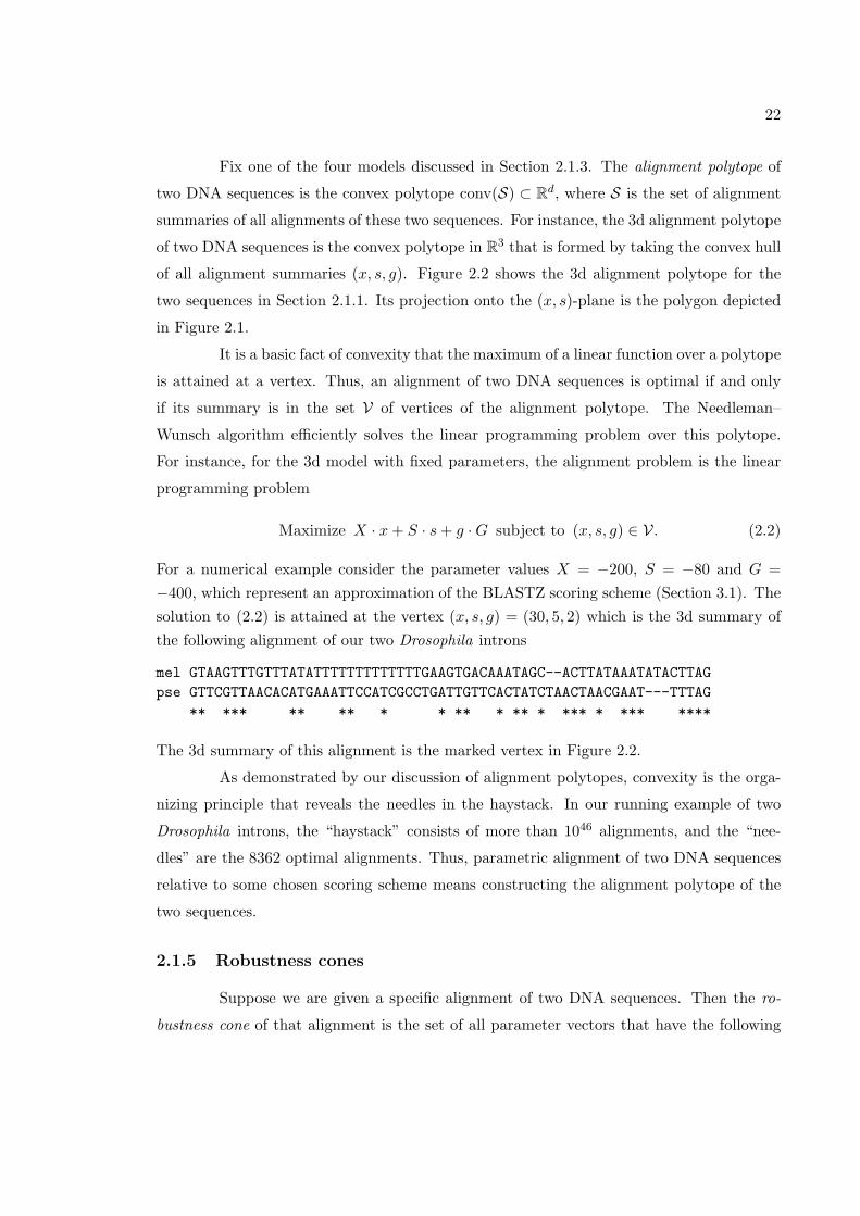
d 2 3 4 5# of vertices 13 76 932 10009

# of edges 13 159 3546 66211# of 2d faces — 85 4208 139723# of 3d faces — — 1594 118797# of 4d faces — — — 35278

Avg. # of edges per vertex 2 4.2 7.6 13.2

Table 2.3: Face numbers of the alignment polytopes for the intron sequences from thebeginning of the Introduction. The average number of edges containing a vertex is theaverage number of linear inequalities bounding a robustness cone.

property: any other alignment that has a different alignment summary is given a lower

score. As a mathematical object, the robustness cone is an open convex polyhedral cone in

the space Rd of free parameters.

An alignment summary is said to be optimal, relative to a given model, if its

robustness cone is not empty. Equivalently, an alignment summary is optimal if there

exists a choice of parameters such that the Needleman–Wunsch algorithm produces only

that alignment summary. Such a parameter choice will be robust, in the sense that if we

make a small enough change in the parameters then the optimal alignment summary will

remain unchanged. Each robustness cone is specified by a finite list of linear inequalities in

the model parameters.

For example, consider the first alignment in the Section 2.1.1. Its 2d alignment

summary is the pair (x, s) = (23, 9), labeled D in Table 2.1. The robustness cone of this

summary is the set of all points (X,S) such that the score 23X + 9S is larger than the

score of all other alignments summaries other than (23, 9). This cone is specified by the two

linear inequalities S > X and 4S < 3X.

If we fix two DNA sequences, then the robustness cones of all the optimal align-

ments define a partition of the parameter space, Rd. That partition is called the alignment

fan of the two DNA sequences. Figure 2.1 shows the (biologically relevant part of the)

alignment fan of two Drosophila introns in the 2d model. While this alignment fan has

only 13 robustness cones, the alignment fan of the same introns has 76 cones for the 3d

model, 932 cones for the 4d model, and 10,009 cones for the 5d model. These are the vertex

numbers in Table 2.3.

24

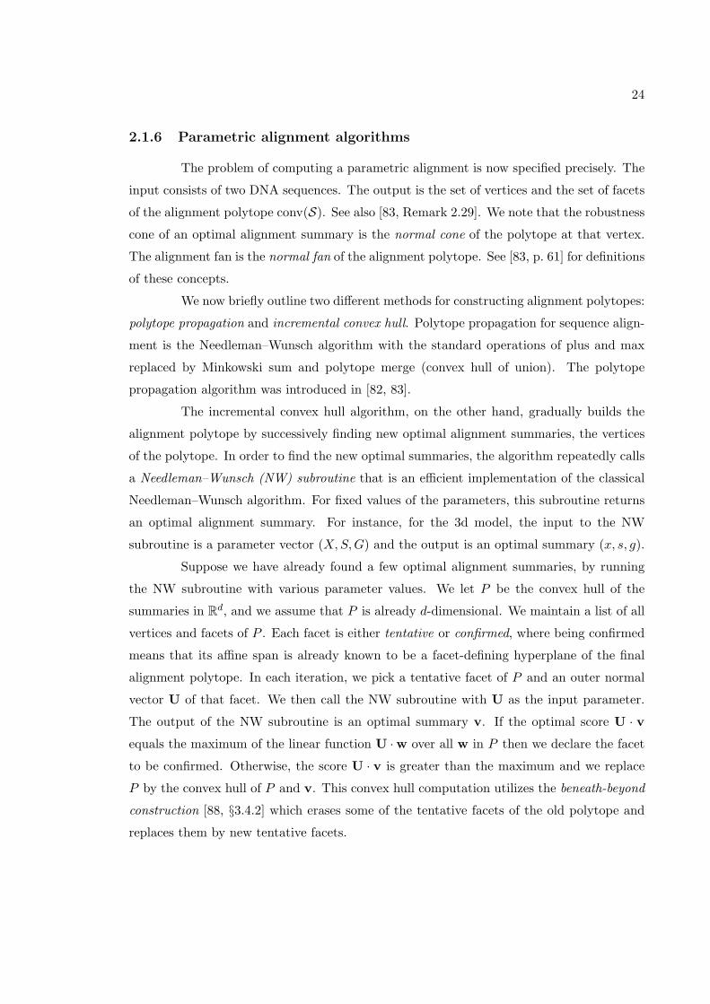
2.1.6 Parametric alignment algorithms

The problem of computing a parametric alignment is now specified precisely. The

input consists of two DNA sequences. The output is the set of vertices and the set of facets

of the alignment polytope conv(S). See also [83, Remark 2.29]. We note that the robustness

cone of an optimal alignment summary is the normal cone of the polytope at that vertex.

The alignment fan is the normal fan of the alignment polytope. See [83, p. 61] for definitions

of these concepts.

We now briefly outline two different methods for constructing alignment polytopes:

polytope propagation and incremental convex hull. Polytope propagation for sequence align-

ment is the Needleman–Wunsch algorithm with the standard operations of plus and max

replaced by Minkowski sum and polytope merge (convex hull of union). The polytope

propagation algorithm was introduced in [82, 83].

The incremental convex hull algorithm, on the other hand, gradually builds the

alignment polytope by successively finding new optimal alignment summaries, the vertices

of the polytope. In order to find the new optimal summaries, the algorithm repeatedly calls

a Needleman–Wunsch (NW) subroutine that is an efficient implementation of the classical

Needleman–Wunsch algorithm. For fixed values of the parameters, this subroutine returns

an optimal alignment summary. For instance, for the 3d model, the input to the NW

subroutine is a parameter vector (X,S,G) and the output is an optimal summary (x, s, g).

Suppose we have already found a few optimal alignment summaries, by running

the NW subroutine with various parameter values. We let P be the convex hull of the

summaries in Rd, and we assume that P is already d-dimensional. We maintain a list of all

vertices and facets of P . Each facet is either tentative or confirmed, where being confirmed

means that its affine span is already known to be a facet-defining hyperplane of the final

alignment polytope. In each iteration, we pick a tentative facet of P and an outer normal

vector U of that facet. We then call the NW subroutine with U as the input parameter.

The output of the NW subroutine is an optimal summary v. If the optimal score U · vequals the maximum of the linear function U ·w over all w in P then we declare the facet

to be confirmed. Otherwise, the score U · v is greater than the maximum and we replace

P by the convex hull of P and v. This convex hull computation utilizes the beneath-beyond

construction [88, §3.4.2] which erases some of the tentative facets of the old polytope and

replaces them by new tentative facets.

25

The algorithm terminates when all facets are confirmed. The current polytope P at

that iteration is the final alignment polytope. The number of iterations of this incremental

convex hull algorithm equals the number of vertices plus the number of facets of the final

polytope P . So for a given model, the running time of the incremental convex hull algorithm

scales linearly in the size of the output. This was confirmed in practice by our computations

described in Chapter 4 (see Table 4.1).

Given an alignment polytope, there are various subsequent computations one may

wish to perform. For instance, we may be interested in the robustness cones at the vertices.

In order to get an irredundant inequality representation of a robustness cone, it suffices to

know the edges emanating from the corresponding vertex. Thus it is useful to also compute

the edge graph of each of our polytopes.

2.2 Statistical alignment

We have seen that parametric alignment allows for the examination of the de-

pendence of optimal alignments on model parameters. Thus far, parametric methods have

only been described for alignment scoring schemes that are not statistically based. In this

section, a statistical alignment model will be given such that every parameter setting is

equivalent to a set of scores for classic Needleman–Wunsch alignment.

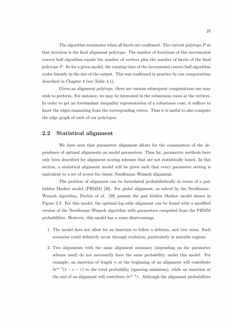
The problem of alignment can be formulated probabilistically in terms of a pair

hidden Markov model (PHMM) [38]. For global alignment, as solved by the Needleman–

Wunsch algorithm, Durbin et al. [38] present the pair hidden Markov model shown in

Figure 2.3. For this model, the optimal log-odds alignment can be found with a modified

version of the Needleman–Wunsch algorithm with parameters computed from the PHMM

probabilities. However, this model has a some shortcomings.

1. The model does not allow for an insertion to follow a deletion, and vice versa. Such

scenarios could definitely occur through evolution, particularly in mutable regions.

2. Two alignments with the same alignment summary (depending on the parameter

scheme used) do not necessarily have the same probability, under this model. For

example, an insertion of length n at the beginning of an alignment will contribute

δεn−1(1 − ε − τ) to the total probability (ignoring emissions), while an insertion at

the end of an alignment will contribute δεn−1τ . Although the alignment probabilities

26

I

D

H

BEGIN END

ε

τ

τ

ε

δ

δ

1-2δ-τ τ

δ

δ

1-ε-τ

1-ε-τ

τ

Figure 2.3: The state transition diagram for the PHMM of [38].

in this example are likely to be very similar, it is desirable to have a model that is

independent of the orientation of the sequences. That is, if we flip the alignment

(perhaps by reverse-complementation in the case of DNA), the probability given by

the model should be the same.

3. A consequence of not giving the same probability to alignments having the same

summary is that the transformation from the PHMM to Needleman–Wunsch involves

some modification to the termination step.

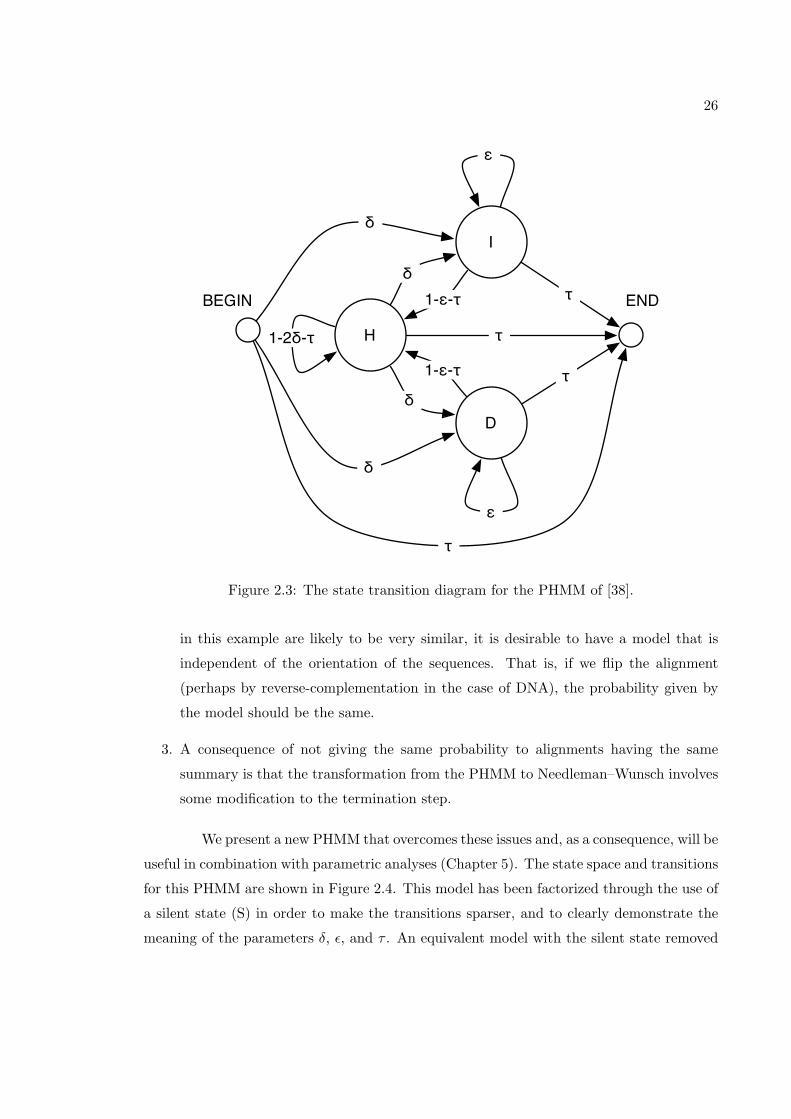
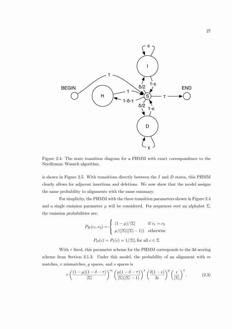
We present a new PHMM that overcomes these issues and, as a consequence, will be

useful in combination with parametric analyses (Chapter 5). The state space and transitions

for this PHMM are shown in Figure 2.4. This model has been factorized through the use of

a silent state (S) in order to make the transitions sparser, and to clearly demonstrate the

meaning of the parameters δ, ε, and τ . An equivalent model with the silent state removed

27

I

D

HBEGIN END

ε

ε

τS

δ/2 1-ε

1-εδ/2

1

1-δ-τ

1

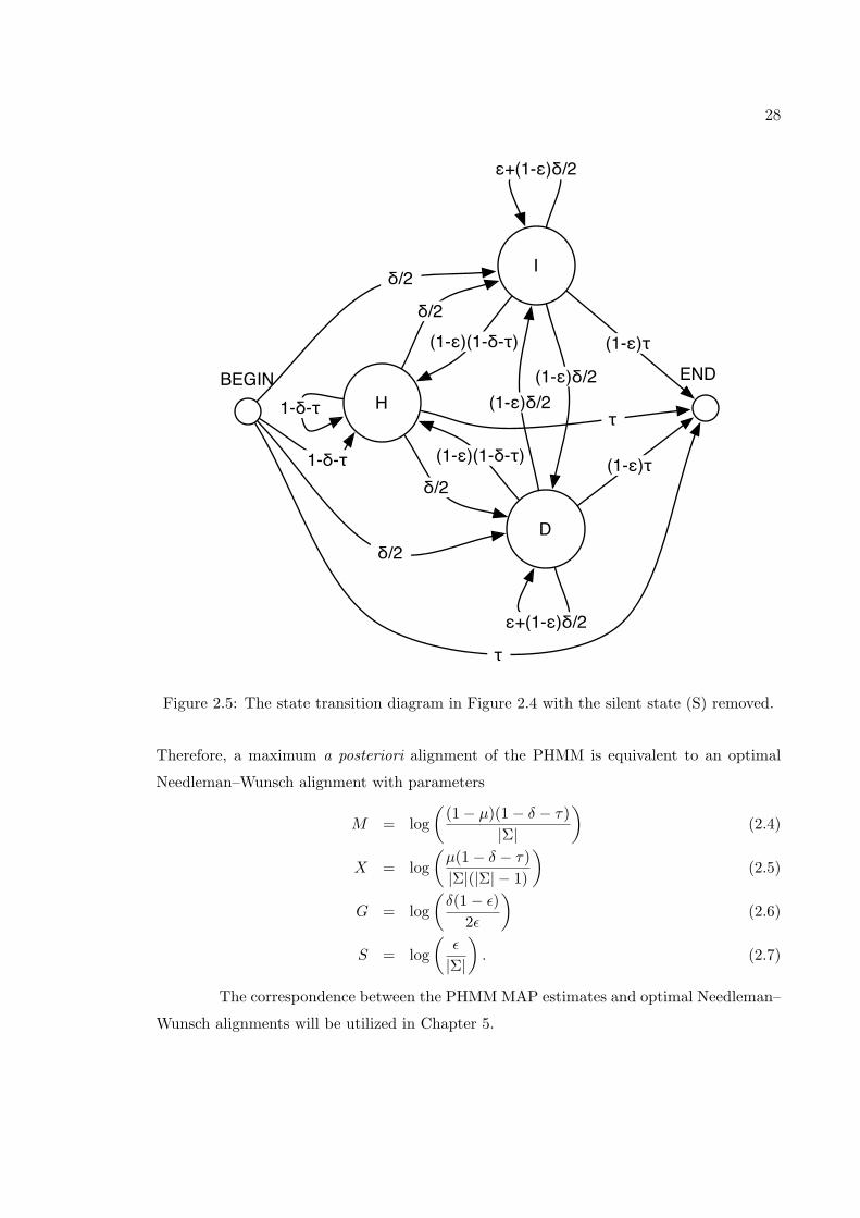
Figure 2.4: The state transition diagram for a PHMM with exact correspondence to theNeedleman–Wunsch algorithm.

is shown in Figure 2.5. With transitions directly between the I and D states, this PHMM

clearly allows for adjacent insertions and deletions. We now show that the model assigns

the same probability to alignments with the same summary.

For simplicity, the PHMM with the three transition parameters shown in Figure 2.4

and a single emission parameter µ will be considered. For sequences over an alphabet Σ,

the emission probabilities are:

PH(c1, c2) =

(1− µ)/|Σ| if c1 = c2

µ/(|Σ|(|Σ| − 1)) otherwise

PD(c) = PI(c) = 1/|Σ|, for all c ∈ Σ

With τ fixed, this parameter scheme for the PHMM corresponds to the 3d scoring

scheme from Section 2.1.3. Under this model, the probability of an alignment with m

matches, x mismatches, g spaces, and s spaces is

τ

((1− µ)(1− δ − τ)

|Σ|

)m (µ(1− δ − τ)|Σ|(|Σ| − 1)

)x (δ(1− ε)

2ε

)g (ε

|Σ|

)s

. (2.3)

28

I

D

HBEGIN END

ε+(1-ε)δ/2

(1-ε)τ

(1-ε)τ

ε+(1-ε)δ/2

δ/2

δ/2

1-δ-τ

δ/2

δ/2

(1-ε)(1-δ-τ)

(1-ε)(1-δ-τ)

τ

(1-ε)δ/2

1-δ-τ

(1-ε)δ/2τ

Figure 2.5: The state transition diagram in Figure 2.4 with the silent state (S) removed.

Therefore, a maximum a posteriori alignment of the PHMM is equivalent to an optimal

Needleman–Wunsch alignment with parameters

M = log(

(1− µ)(1− δ − τ)|Σ|

)(2.4)

X = log(µ(1− δ − τ)|Σ|(|Σ| − 1)

)(2.5)

G = log(δ(1− ε)

2ε

)(2.6)

S = log(ε

|Σ|

). (2.7)

The correspondence between the PHMM MAP estimates and optimal Needleman–

Wunsch alignments will be utilized in Chapter 5.

29

Chapter 3

Multiple whole-genome alignment:

Mercator

A central problem in the comparison of multiple whole genome sequences is ho-

mology mapping, which is the identification of sets of homologous segments among multiple

genomes. We present a solution to this problem that focuses on monotopoorthology, a

one-to-one subrelation of orthology introduced in Chapter 1. Our methods for identifying

monotopoorthologous segments and locating evolutionary breakpoints are based on graph

theoretical frameworks, including the formalism of undirected graphical models. By effec-

tively making use of information from multiple genomes to identify monotopoorthologous

segments and their bounding breakpoints, we are able to produce homology maps that im-

prove on pairwise maps. In an analysis of four mammalian genomes, we show that existing

pairwise alignment strategies map 3% of exons inconsistently, 24.8% of which we are able

to correct using our homology mapping methods. An additional feature of our method is

the ability to comparatively scaffold assemblies that are not yet mapped to chromosomes.

We demonstrate this by comparatively assembling contigs from the human, mouse and rat

genome with few incorrect joins and high coverage of the genomes. An implementation of

our method, Mercator, is freely available and is fast enough to be run on a single work-

station. It is currently being used to guide nucleotide-level multiple alignments of whole

genomes and for genome evolution studies.

30

3.1 Motivation

Since the completion of the first draft assemblies of the human genome [66, 108],

technological advances and lower costs have resulted in the sequencing of many whole verte-

brate genomes, as well as numerous non-vertebrate genomes. At the time of writing, whole

genome sequence assemblies have been produced for 17 vertebrate species, 8 of which have

assemblies into full chromosomes. Projects such as the Mammalian Genome Project [73]

and the recent sequencing of 12 Drosophila species [26] will provide us with a large number

of additional genomes to analyze using the tools of comparative genomics.

An important first step in comparing all of these genomes is to determine the

large-scale correspondences between them. At a low resolution, one can identify (with a

microscope) related chromosomes from two species using chromosome painting techniques

such as Zoo-FISH [93]. These techniques allow for the detection of conserved synteny : the

state of elements on the same chromosome in one genome having their homologs occurring

on the same chromosome in another genome. When markers, such as genes, have been

mapped and ordered on multiple genomes, comparative genetic maps can be created. Such

maps have resolutions that depend on the density of markers used and allow for the detection

of conserved segments: segments in multiple genomes containing homologous markers that

occur in the same order in each genome [79].

With the sequencing of whole genomes, we are now able to produce comparative

maps at the nucleotide level. In addition to protein coding genes for which we have genomic

coordinates, we can also use conserved non-coding sequence as markers. For a set of fully

sequenced genomes, we would like to divide the genome sequences into coordinate-based

segments and then determine evolutionary relationships among them. We call the result

of such an analysis a homology map. When the segments are defined in such a way that

homologous segments are colinear, the map is called a colinear homology map. Of particular

interest are the construction of orthology maps which specify only a subset of evolutionary

relationships between genomic segments.

Homology maps are important for many kinds of downstream analyses. For exam-

ple, if one would like to obtain a nucleotide-level alignment of a set of genomes, one simply

feeds the sets of homologous segments established by the map to alignment programs such

as DIALIGN [77], MAVID [12], MLAGAN [15], or TBA [8]. Another analysis that requires

a colinear homology map, but not a nucleotide-level alignment, is that of determining the

31

history of genomic rearrangements [86, 78]. The combination of these two analyses gives a

proposed evolutionary history for every position in every genome and allows for the inference

of ancestral genome sequence [7].

In this chapter, we present a method for constructing colinear monotopoorthology

maps between multiple whole genomes. We first introduce a series of molecular evolution

definitions to explain what such a map represents. We then present the details of our

algorithms for constructing maps, as they are implemented in the program Mercator. Lastly,

we give some results that demonstrate the performance of Mercator on four large eukaryotic

genomes. Mercator is shown to produce accurate maps, to assemble genomes comparatively,

and to locate breakpoints between rearranged orthologous segments effectively.

3.2 Related Work

3.2.1 Pairwise maps

Much work has been done on the identification of homologous segments between

pairs of genomes. In general, these methods comprise three steps:

1. identification of local alignments between genome sequences,

2. clustering of alignments by genomic position and orientation, and

3. filtering and classification of clusters to predict homologous relationships.

Local alignments between genomes can be obtained through all-vs-all comparisons

of protein coding regions using programs such as BLAST and BLAT [1, 61] or from nu-

cleotide alignment programs that can be used at the whole-genome scale [61, 65, 68, 95].

Without using genomic context information (step two), several methods predict orthology

and paralogy relations between the proteomes of multiple genomes [102, 67, 89]. Combined

with genomic coordinates for the genes encoding the proteins given as input, these methods

can be used to produce gene-based homology maps.

Although one can predict homology relationships between proteins without utiliz-

ing the positions of their coding genes, genomic context can provide valuable information

for inferring the evolutionary relationships between genomic segments. Since rearrange-

ment events undergone by genomes during evolution are rare, neighboring elements in one

32

genome tend to have homologs that are neighbors in other genomes [105]. Other methods

described here take advantage of genomic context in some fashion.

A common approach used by genome sequencing projects (e.g., [100]) for deter-

mining orthology maps is to first identify best bidirectional hits, or SymBets [63], between

the protein coding genes of two genomes. SymBets are assumed to be orthologs and addi-

tional orthology relationships are determined based on adjacencies to genes participating

in SymBets. This strategy has been extended in various ways. For human and mouse,

nucleotide-level “syntenic” anchors and function annotations are additionally used to pre-

dict orthologous genes [116]. For yeast, the SymBet strategy was extended to give subsets

of orthologous proteins in cases where recent duplications have led to many-to-one or many-

to-many orthologous relationships [60].

Of the orthology mapping methods that use local nucleotide alignments, the most

widely-used are based on the chaining of local alignments [58, 62, 65, 86, 101]. Although

all of these methods chain local alignments, they are quite different at all three steps of

the orthology mapping process and give different types of output. For example, the nets

produced by [62] make up a many-to-one orthology map between a reference and query

genome, while the output of [58] is a one-to-one orthology map. We will distinguish be-

tween such orthology maps in Section 3.3. Methods that do not use chaining and that rely

on nucleotide anchors unique to a pair of genomes are given in [112] and [69]. More re-

cently, methods that take into account a parsimonious series of rearrangement events while

predicting orthologous segments have been proposed [23, 24]. For a more detailed review

of some of these methods, see [2, 36].

Thus far, we have mentioned methods that attempt to identify orthologous re-

lationships between genomes. There are many others that predict homologous genomic

segments without specifying precisely how the segments are related. The majority of these

methods use gene comparison data. Some identify genomic segments containing a significant

number of colinear or clustered homologous genes [18, 107, 53, 52]. Others are formulated

to locate diagonals within gene dot plots [20, 50]. The diagonal locating ability of [20] has

been used in [19] to construct maps that distinguish between orthologous and paralogous

segments. Lastly, a unique method utilizing the formalism of Markov random fields and

capable of using either gene or nucleotide-level alignments was developed by [21].

33

3.2.2 Multiple maps

Although a large number of pairwise homology mapping programs are available,

few methods have been developed for mapping between three or more genomes simultane-

ously. Simply combining pairwise maps is not sufficient because, just as in the multiple

sequence alignment problem, pairwise maps are often not consistent. We demonstrate the

inconsistency of whole-genome alignments based on pairwise maps in Section 3.5.2. Sec-

tion 1.4.2 reviewed a number of multiple genome mapping methods that have been used

on large genomes. Other mappers of note include a method that uses Gibbs-like sampler

to detect orthologous segments in multiple diverged genomes [74], and a method that finds

conserved gene orders in multiple genomes once orthology has been assigned [85].

Visualizing multiple homology maps presents other challenges. The K-Browser

[22] and ENSEMBL’s “alignslice view” [5] allow for the browsing of a one-to-one orthology

mapping and nucleotide-level alignment. SyntenyVista [55] is a well-prototyped program

for visualizing orthology between multiple genomes at a variety of scales. UCSC’s Genome

Browser also has tracks for visualizing the nets and chains produced by [62].

3.3 Definitions

The literature on homology mapping methods is full of ambiguous use of termi-

nology. Methods are also frequently used to define the desired output making it difficult to

ascertain the biological relevance of the maps that are produced. These problems are the

result of a lack of terminology for describing the complex evolutionary relationships that

form the basis of homology. In Section 1.3.2, we introduced a series of new terms that are

helpful in describing the output of homology mapping methods, and in particular, the out-

put of the method presented here. We wish to emphasize that the new terms are based on

biological considerations and have not simply been invented to explain algorithmic output.

We introduce two terms to define the correspondence that our method and others

determine between a set of genomes.

Definition 5 (Colinear monotopoorthology) Genomic segments S1 and S2 are colin-

ear monotopoorthologous if they are monotopoorthologous and the monotopoorthologous

nucleotides contained within the segments occur in the same order.

34

Definition 6 (Colinear monotopoorthology map) A colinear monotopoorthology

map is a set of genomic segment sets, each consisting of pairwise colinear monotopoorthol-

ogous segments.

For a set of multiple whole genomes, a colinear monotopoorthology map is what many have

referred to as a “synteny map,” and is the primary output of the method that we present.

3.4 Algorithms

3.4.1 Overview

We now describe our algorithms for constructing a colinear monotopoorthology

map between multiple whole genomes. These algorithms are implemented in the program

Mercator. Mercator’s primary input is a set of k genomes, and its primary output is a

colinear monotopoorthology map. A map consists of a collection of segment sets, with all

segments in a given set considered to be colinear monotopoorthologs of each other. Each

segment set contains between two and k segments, with at most one segment from each

genome.

The strategy employed by our method is to consider only certain intervals, or an-

chors, in each genome in order to determine monotopoorthology relationships. Although

an anchor may be any genomic interval, convenient intervals to use are genes, exons, or

intervals that are part of maximally unique matches (MUMs) [65]. The only restriction

on anchors is that they do not overlap. Anchors are compared in an all-vs-all fashion to

produce a set of significant pairwise hits between anchor sequences. Using sets of input

anchors and hits, Mercator first identifies colinear monotopoorthologous segments by iden-

tifying neighboring cliques of anchors. During the joining of neighboring cliques, Mercator

is capable of comparatively assembling genomes whose contigs have not been assigned to

chromosomal positions. The colinear monotopoorthology pre-map established by the first

step is refined by locating good breakpoints in between adjacent segments. The location

of breakpoints is formulated as finding a maximum a posteriori configuration of a cer-

tain undirected graphical model. A schematic specifying the inputs, outputs, and primary

components of Mercator is shown in Figure 3.1.

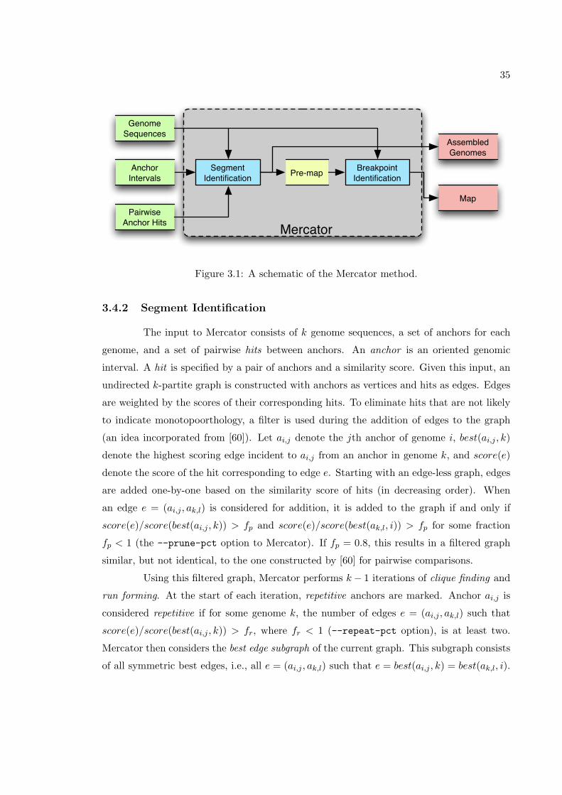
35

Segment Identification

Breakpoint Identification

Genome Sequences

Anchor Intervals

Pairwise Anchor Hits

Pre-map

Map

Mercator

Assembled Genomes

Figure 3.1: A schematic of the Mercator method.

3.4.2 Segment Identification

The input to Mercator consists of k genome sequences, a set of anchors for each

genome, and a set of pairwise hits between anchors. An anchor is an oriented genomic

interval. A hit is specified by a pair of anchors and a similarity score. Given this input, an

undirected k-partite graph is constructed with anchors as vertices and hits as edges. Edges

are weighted by the scores of their corresponding hits. To eliminate hits that are not likely

to indicate monotopoorthology, a filter is used during the addition of edges to the graph

(an idea incorporated from [60]). Let ai,j denote the jth anchor of genome i, best(ai,j , k)

denote the highest scoring edge incident to ai,j from an anchor in genome k, and score(e)

denote the score of the hit corresponding to edge e. Starting with an edge-less graph, edges

are added one-by-one based on the similarity score of hits (in decreasing order). When

an edge e = (ai,j , ak,l) is considered for addition, it is added to the graph if and only if

score(e)/score(best(ai,j , k)) > fp and score(e)/score(best(ak,l, i)) > fp for some fraction

fp < 1 (the --prune-pct option to Mercator). If fp = 0.8, this results in a filtered graph

similar, but not identical, to the one constructed by [60] for pairwise comparisons.

Using this filtered graph, Mercator performs k− 1 iterations of clique finding and

run forming. At the start of each iteration, repetitive anchors are marked. Anchor ai,j is

considered repetitive if for some genome k, the number of edges e = (ai,j , ak,l) such that

score(e)/score(best(ai,j , k)) > fr, where fr < 1 (--repeat-pct option), is at least two.

Mercator then considers the best edge subgraph of the current graph. This subgraph consists

of all symmetric best edges, i.e., all e = (ai,j , ak,l) such that e = best(ai,j , k) = best(ak,l, i).

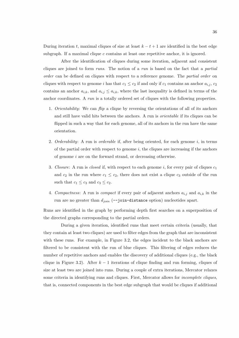
36

During iteration t, maximal cliques of size at least k − t+ 1 are identified in the best edge

subgraph. If a maximal clique c contains at least one repetitive anchor, it is ignored.

After the identification of cliques during some iteration, adjacent and consistent

cliques are joined to form runs. The notion of a run is based on the fact that a partial

order can be defined on cliques with respect to a reference genome. The partial order on

cliques with respect to genome i has that c1 ≤ c2 if and only if c1 contains an anchor ai,j , c2

contains an anchor ai,k, and ai,j ≤ ai,k, where the last inequality is defined in terms of the

anchor coordinates. A run is a totally ordered set of cliques with the following properties.

1. Orientability : We can flip a clique by reversing the orientations of all of its anchors

and still have valid hits between the anchors. A run is orientable if its cliques can be

flipped in such a way that for each genome, all of its anchors in the run have the same

orientation.

2. Orderability : A run is orderable if, after being oriented, for each genome i, in terms

of the partial order with respect to genome i, the cliques are increasing if the anchors

of genome i are on the forward strand, or decreasing otherwise.

3. Closure: A run is closed if, with respect to each genome i, for every pair of cliques c1

and c2 in the run where c1 ≤ c2, there does not exist a clique c3 outside of the run

such that c1 ≤ c3 and c3 ≤ c2.

4. Compactness: A run is compact if every pair of adjacent anchors ai,j and ai,k in the

run are no greater than djoin (--join-distance option) nucleotides apart.

Runs are identified in the graph by performing depth first searches on a superposition of

the directed graphs corresponding to the partial orders.

During a given iteration, identified runs that meet certain criteria (usually, that

they contain at least two cliques) are used to filter edges from the graph that are inconsistent

with these runs. For example, in Figure 3.2, the edges incident to the black anchors are

filtered to be consistent with the run of blue cliques. This filtering of edges reduces the

number of repetitive anchors and enables the discovery of additional cliques (e.g., the black

clique in Figure 3.2). After k − 1 iterations of clique finding and run forming, cliques of

size at least two are joined into runs. During a couple of extra iterations, Mercator relaxes

some criteria in identifying runs and cliques. First, Mercator allows for incomplete cliques,

that is, connected components in the best edge subgraph that would be cliques if additional

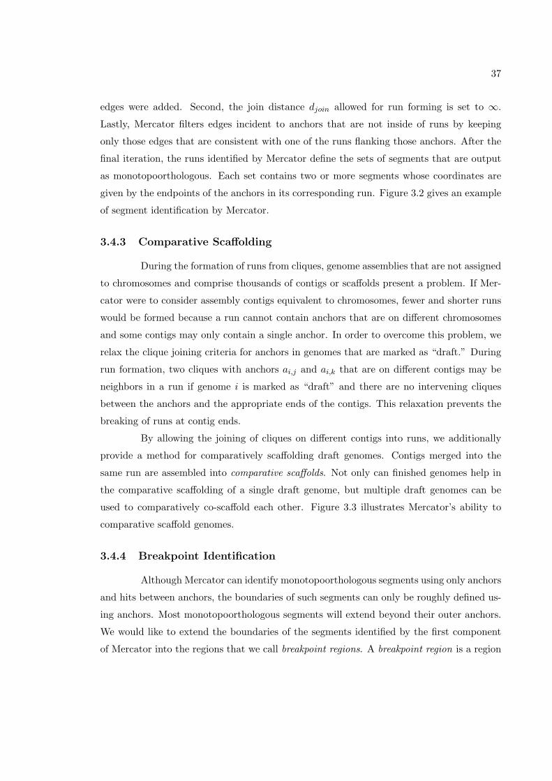
37

edges were added. Second, the join distance djoin allowed for run forming is set to ∞.

Lastly, Mercator filters edges incident to anchors that are not inside of runs by keeping

only those edges that are consistent with one of the runs flanking those anchors. After the

final iteration, the runs identified by Mercator define the sets of segments that are output

as monotopoorthologous. Each set contains two or more segments whose coordinates are

given by the endpoints of the anchors in its corresponding run. Figure 3.2 gives an example

of segment identification by Mercator.

3.4.3 Comparative Scaffolding

During the formation of runs from cliques, genome assemblies that are not assigned

to chromosomes and comprise thousands of contigs or scaffolds present a problem. If Mer-

cator were to consider assembly contigs equivalent to chromosomes, fewer and shorter runs

would be formed because a run cannot contain anchors that are on different chromosomes

and some contigs may only contain a single anchor. In order to overcome this problem, we

relax the clique joining criteria for anchors in genomes that are marked as “draft.” During

run formation, two cliques with anchors ai,j and ai,k that are on different contigs may be

neighbors in a run if genome i is marked as “draft” and there are no intervening cliques

between the anchors and the appropriate ends of the contigs. This relaxation prevents the

breaking of runs at contig ends.

By allowing the joining of cliques on different contigs into runs, we additionally

provide a method for comparatively scaffolding draft genomes. Contigs merged into the

same run are assembled into comparative scaffolds. Not only can finished genomes help in

the comparative scaffolding of a single draft genome, but multiple draft genomes can be

used to comparatively co-scaffold each other. Figure 3.3 illustrates Mercator’s ability to

comparative scaffold genomes.

3.4.4 Breakpoint Identification

Although Mercator can identify monotopoorthologous segments using only anchors

and hits between anchors, the boundaries of such segments can only be roughly defined us-

ing anchors. Most monotopoorthologous segments will extend beyond their outer anchors.

We would like to extend the boundaries of the segments identified by the first component

of Mercator into the regions that we call breakpoint regions. A breakpoint region is a region

38

A

B

C

Figure 3.2: Identification of monotopoorthologous segments by Mercator. The long greybars represent segments from three genomes, colored rectangles denote anchors within thesesegments, and lines incident to anchors represent hits (an arrowhead indicates that the otheranchor is not within the shown segments). High-scoring hits are shown as solid lines, whileweaker hits are drawn as dotted lines. (A) Repetitive anchors (black) are marked andthree-cliques (blue and red) are identified. (B) Runs formed by the red and blue anchorsare identified and edges inconsistent with these runs are filtered. (C) Two-cliques andcliques including anchors previously considered repetitive are discovered and included intoruns.

39

A

B

Figure 3.3: Mercator can comparatively scaffold genomes. Grey bars are segments fromthree genomes, yellow regions denote a monotopoorthologous segment set, as discoveredthrough examination of anchors (colored rectangles) and hits (lines between anchors). (A)Two finished genomes help to scaffold (indicated by dotted lines) a third (top) genome thatis still in scaffolds. (B) Three draft genomes scaffold each other. Note that in this scenario,information from all three genomes is required to join the adjacent contigs.

in between two neighboring segments that could not be joined together due to a rearrange-

ment in at least one of the genomes. We call the position in such a region at which a

rearrangement event caused a disruption of colinearity the breakpoint. Figure 3.4A shows

the segments of a monotopoorthology pre-map and the breakpoint regions in between them.

Mercator improves the pre-map by choosing a good breakpoint in each breakpoint region

and extending the flanking segments to the breakpoint position.

Breakpoint Model

We formalize the problem of finding breakpoints in terms of identifying a maximum

a posteriori (MAP) configuration of a certain undirected graphical model. The structure

of the graphical model is defined by the monotopoorthology pre-map. Let ri,j denote the

jth breakpoint region in genome i and let Bi,j be the hidden random variable representing

the position of the breakpoint in ri,j . Each random variable is a node in the graphical

model. The position of the breakpoint in ri,j is dependent on the positions of the break-

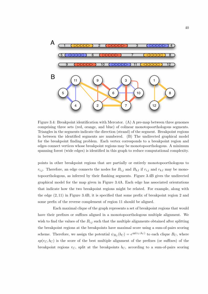
40

A

B

1 2 3 4

5 6 7 8

1211109

1

2

6

7

3

8

4

5

9

10

11

12

Figure 3.4: Breakpoint identification with Mercator. (A) A pre-map between three genomescomprising three sets (red, orange, and blue) of colinear monotopoorthologous segments.Triangles in the segments indicate the direction (strand) of the segment. Breakpoint regionsin between the identified segments are numbered. (B) The undirected graphical modelfor the breakpoint finding problem. Each vertex corresponds to a breakpoint region andedges connect vertices whose breakpoint regions may be monotopoorthologous. A minimumspanning forest (wide edges) is identified in this graph to reduce computational complexity.

points in other breakpoint regions that are partially or entirely monotopoorthologous to

ri,j . Therefore, an edge connects the nodes for Bi,j and Bk,l if ri,j and rk,l may be mono-

topoorthologous, as inferred by their flanking segments. Figure 3.4B gives the undirected

graphical model for the map given in Figure 3.4A. Each edge has associated orientations

that indicate how the two breakpoint regions might be related. For example, along with

the edge (2, 11) in Figure 3.4B, it is specified that some prefix of breakpoint region 2 and

some prefix of the reverse complement of region 11 should be aligned.

Each maximal clique of the graph represents a set of breakpoint regions that would

have their prefixes or suffixes aligned in a monotopoorthologous multiple alignment. We

wish to find the values of the Bi,j such that the multiple alignments obtained after splitting

the breakpoint regions at the breakpoints have maximal score using a sum-of-pairs scoring

scheme. Therefore, we assign the potential ψBC(bC) = esp(rC ,bC) to each clique BC , where

sp(rC , bC) is the score of the best multiple alignment of the prefixes (or suffixes) of the

breakpoint regions rC , split at the breakpoints bC , according to a sum-of-pairs scoring

41

scheme. The probability distribution of the whole model is thus

p(b) =1Z

∏C∈C

ψBC(bC),

where Z is a normalizing constant and C is the set of all maximal cliques in the graph.

Breakpoint Inference

Ideally, we would like to find the MAP values for the breakpoints b under the

model just described. However, due to the high connectivity of the graph and the difficulty

of multiple alignment, exact inference appears to be computationally infeasible. Therefore,

we use a series of heuristics to reduce the complexity of the problem while retaining the

most important constraints.

We first modify the model to avoid having to compute multiple alignments. Instead

of assigning potentials to maximal cliques, we assign potentials to edges only. These depend

on pairwise alignment scores. If optimal pairwise alignments were always consistent with an

optimal multiple alignment, then this formulation would be equivalent, but this is unlikely

to be the case. However, we believe that pairwise alignments can provide the majority of

the information regarding breakpoint locations and that the heuristic is therefore justified.

A second computational challenge results from the size of the cliques in the graph

and the number of breakpoints that we must consider in each region. To reduce the com-

plexity further, we eliminate edges from the graph by only considering a minimum spanning

forest (MSF) in the graph (i.e., a set of minimum spanning trees, one for each connected

component of the graph), where the edges are weighted by phylogenetic distances. To find a

MSF, Each edge (Bi,j , Bk,l) is weighted by distance(i, k), which provides a distance measure

between genomes i and k. The MSF will generally include only the shortest edges, which

are likely to be the most informative because the sequences connected by such edges have

had the least amount of time to diverge.

The calculation and storage of the edge potentials presents another difficulty in

MAP estimation for this model. Each potential requires computing score(ri,j , rk,l, bi,j , bk,l),

the optimal pairwise alignment score of aligning a prefix specified by bi,j of ri,j to a prefix

specified by bk,l of rk,l (both regions possibly reverse complemented), for all length(ri,j)×length(rk,l) combinations of breakpoints. This computation can be done with a single pass of

the Needleman–Wunsch algorithm, but requires length(ri,j)× length(rk,l) time and space.

42

Therefore we approximate such prefix scores by calculating and storing a single optimal

pairwise alignment of the breakpoint regions. Given an optimal pairwise alignment of ri,j

and rk,l, we approximate score(ri,j , rk,l, bi,j , bk,l) by the score of the prefix sub-alignment

obtained by cutting at bi,j and bk,l. Pairwise alignments may be quickly calculated using

programs such as MAVID [12] or LAGAN [15].

After construction of the breakpoint region graph, identification of a MSF, and

computation of pairwise alignments for edges in the MSF, the computation of optimal

breakpoint positions can be obtained using the standard max-product algorithm for tree

graphical models. As an additional speed-up to the algorithm, we run the algorithm for

several iterations, considering at most p possible values for each breakpoint at a given

iteration. Suppose that at iteration t we consider b1, b2, . . . , bp as possible positions for a

breakpoint and find that bi, i ∈ [1, p] is the best of these positions. Then at iteration t+ 1,

we restrict the range of the breakpoint to be [bi−1, bi+1]. During the last iteration of the

algorithm, the intervals that we consider for each breakpoint all have size at most m. This

restriction allows us to compute good breakpoints in time O(np2 log `+m log n), excluding

time for computing pairwise alignments, where n is the number of nodes, m is the number

of initial edges in the graph, and ` is the length of the longest breakpoint region.

3.5 Results

The evaluation of genomic alignment methods remains a difficult task, both for

nucleotide-level alignment and higher-level maps. Unlike protein alignment, where reference

alignments are often constructed using structural information, there are no such benchmarks

for nucleotide alignment. Although whole-genome evolutionary simulation might be an

option, our limited understanding of genome evolution makes it difficult to define and

set parameters. Therefore, without a gold standard with which to evaluate Mercator, we

compared and contrasted its maps with whole-genome pairwise alignments constructed by

other methods. Comparison with one of the other multiple map (Section 3.2.2) methods was

not feasible because either the software was not made freely available, the input and output

of the method was not comparable, or the method was too computationally expensive for

the data sets used here.

We therefore based our analyses on comparisons to the widely used pairwise net

alignments of the human, mouse, rat and dog genomes made available at the UCSC Genome

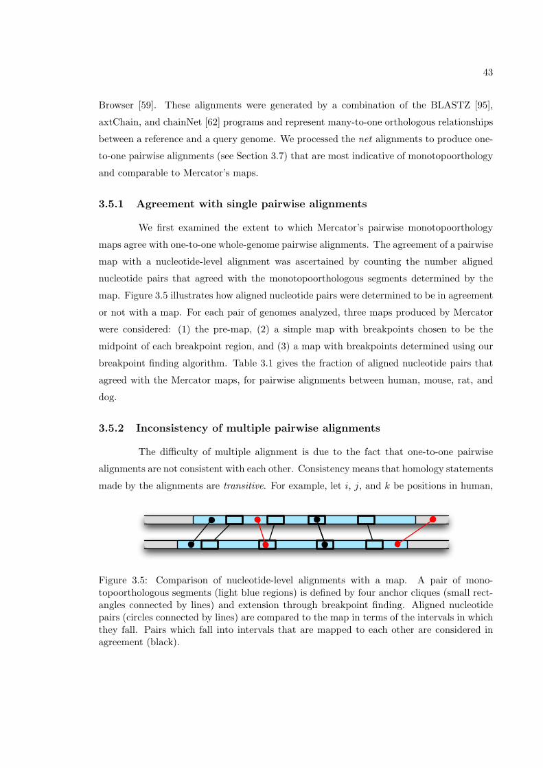
43

Browser [59]. These alignments were generated by a combination of the BLASTZ [95],

axtChain, and chainNet [62] programs and represent many-to-one orthologous relationships

between a reference and a query genome. We processed the net alignments to produce one-

to-one pairwise alignments (see Section 3.7) that are most indicative of monotopoorthology

and comparable to Mercator’s maps.

3.5.1 Agreement with single pairwise alignments

We first examined the extent to which Mercator’s pairwise monotopoorthology

maps agree with one-to-one whole-genome pairwise alignments. The agreement of a pairwise

map with a nucleotide-level alignment was ascertained by counting the number aligned

nucleotide pairs that agreed with the monotopoorthologous segments determined by the

map. Figure 3.5 illustrates how aligned nucleotide pairs were determined to be in agreement

or not with a map. For each pair of genomes analyzed, three maps produced by Mercator

were considered: (1) the pre-map, (2) a simple map with breakpoints chosen to be the

midpoint of each breakpoint region, and (3) a map with breakpoints determined using our

breakpoint finding algorithm. Table 3.1 gives the fraction of aligned nucleotide pairs that

agreed with the Mercator maps, for pairwise alignments between human, mouse, rat, and

dog.

3.5.2 Inconsistency of multiple pairwise alignments

The difficulty of multiple alignment is due to the fact that one-to-one pairwise

alignments are not consistent with each other. Consistency means that homology statements

made by the alignments are transitive. For example, let i, j, and k be positions in human,

Figure 3.5: Comparison of nucleotide-level alignments with a map. A pair of mono-topoorthologous segments (light blue regions) is defined by four anchor cliques (small rect-angles connected by lines) and extension through breakpoint finding. Aligned nucleotidepairs (circles connected by lines) are compared to the map in terms of the intervals in whichthey fall. Pairs which fall into intervals that are mapped to each other are considered inagreement (black).

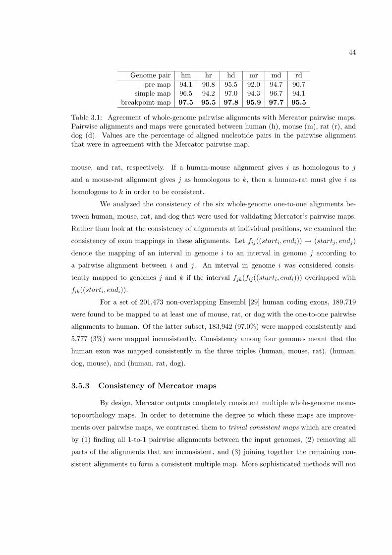
44

Genome pair hm hr hd mr md rdpre-map 94.1 90.8 95.5 92.0 94.7 90.7

simple map 96.5 94.2 97.0 94.3 96.7 94.1breakpoint map 97.5 95.5 97.8 95.9 97.7 95.5

Table 3.1: Agreement of whole-genome pairwise alignments with Mercator pairwise maps.Pairwise alignments and maps were generated between human (h), mouse (m), rat (r), anddog (d). Values are the percentage of aligned nucleotide pairs in the pairwise alignmentthat were in agreement with the Mercator pairwise map.

mouse, and rat, respectively. If a human-mouse alignment gives i as homologous to j

and a mouse-rat alignment gives j as homologous to k, then a human-rat must give i as

homologous to k in order to be consistent.

We analyzed the consistency of the six whole-genome one-to-one alignments be-

tween human, mouse, rat, and dog that were used for validating Mercator’s pairwise maps.

Rather than look at the consistency of alignments at individual positions, we examined the

consistency of exon mappings in these alignments. Let fij((starti, endi)) → (startj , endj)

denote the mapping of an interval in genome i to an interval in genome j according to

a pairwise alignment between i and j. An interval in genome i was considered consis-

tently mapped to genomes j and k if the interval fjk(fij((starti, endi))) overlapped with

fik((starti, endi)).

For a set of 201,473 non-overlapping Ensembl [29] human coding exons, 189,719

were found to be mapped to at least one of mouse, rat, or dog with the one-to-one pairwise

alignments to human. Of the latter subset, 183,942 (97.0%) were mapped consistently and

5,777 (3%) were mapped inconsistently. Consistency among four genomes meant that the

human exon was mapped consistently in the three triples (human, mouse, rat), (human,

dog, mouse), and (human, rat, dog).

3.5.3 Consistency of Mercator maps

By design, Mercator outputs completely consistent multiple whole-genome mono-

topoorthology maps. In order to determine the degree to which these maps are improve-

ments over pairwise maps, we contrasted them to trivial consistent maps which are created

by (1) finding all 1-to-1 pairwise alignments between the input genomes, (2) removing all

parts of the alignments that are inconsistent, and (3) joining together the remaining con-

sistent alignments to form a consistent multiple map. More sophisticated methods will not

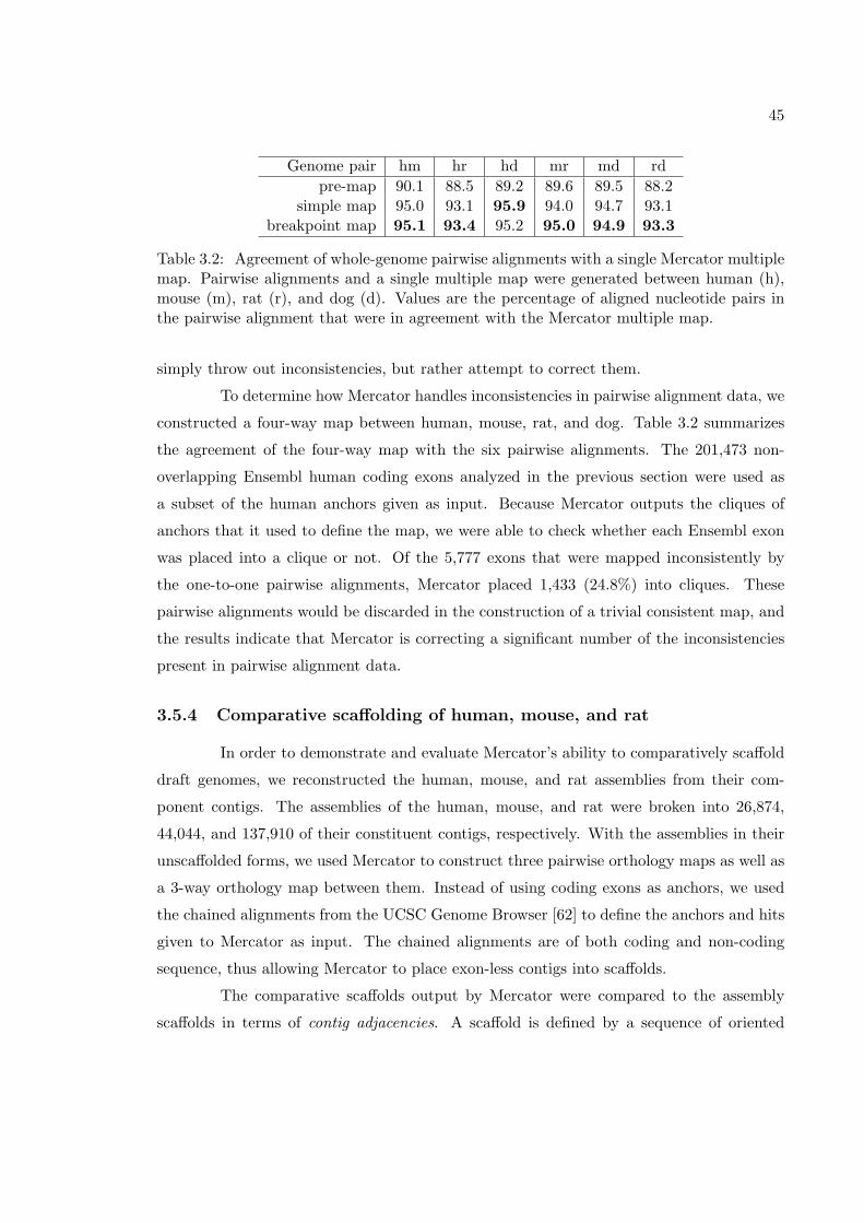
45

Genome pair hm hr hd mr md rdpre-map 90.1 88.5 89.2 89.6 89.5 88.2

simple map 95.0 93.1 95.9 94.0 94.7 93.1breakpoint map 95.1 93.4 95.2 95.0 94.9 93.3

Table 3.2: Agreement of whole-genome pairwise alignments with a single Mercator multiplemap. Pairwise alignments and a single multiple map were generated between human (h),mouse (m), rat (r), and dog (d). Values are the percentage of aligned nucleotide pairs inthe pairwise alignment that were in agreement with the Mercator multiple map.

simply throw out inconsistencies, but rather attempt to correct them.

To determine how Mercator handles inconsistencies in pairwise alignment data, we

constructed a four-way map between human, mouse, rat, and dog. Table 3.2 summarizes

the agreement of the four-way map with the six pairwise alignments. The 201,473 non-

overlapping Ensembl human coding exons analyzed in the previous section were used as

a subset of the human anchors given as input. Because Mercator outputs the cliques of

anchors that it used to define the map, we were able to check whether each Ensembl exon

was placed into a clique or not. Of the 5,777 exons that were mapped inconsistently by

the one-to-one pairwise alignments, Mercator placed 1,433 (24.8%) into cliques. These

pairwise alignments would be discarded in the construction of a trivial consistent map, and

the results indicate that Mercator is correcting a significant number of the inconsistencies

present in pairwise alignment data.

3.5.4 Comparative scaffolding of human, mouse, and rat

In order to demonstrate and evaluate Mercator’s ability to comparatively scaffold

draft genomes, we reconstructed the human, mouse, and rat assemblies from their com-

ponent contigs. The assemblies of the human, mouse, and rat were broken into 26,874,

44,044, and 137,910 of their constituent contigs, respectively. With the assemblies in their

unscaffolded forms, we used Mercator to construct three pairwise orthology maps as well as

a 3-way orthology map between them. Instead of using coding exons as anchors, we used

the chained alignments from the UCSC Genome Browser [62] to define the anchors and hits

given to Mercator as input. The chained alignments are of both coding and non-coding

sequence, thus allowing Mercator to place exon-less contigs into scaffolds.

The comparative scaffolds output by Mercator were compared to the assembly

scaffolds in terms of contig adjacencies. A scaffold is defined by a sequence of oriented

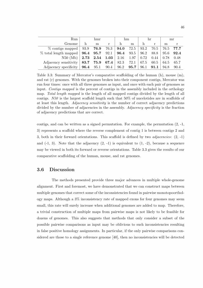
46

Run hmr hm hr mrGenome h m r h m h r m r

% contigs mapped 93.9 76.9 76.3 94.0 72.5 93.2 70.5 76.5 77.7% total length mapped 96.4 95.7 92.1 96.4 93.5 96.2 88.8 95.6 92.4

N50 (Mb) 2.73 2.54 1.03 2.16 1.97 0.72 0.44 0.78 0.48Adjacency sensitivity 83.7 75.9 67.4 82.3 72.1 67.5 60.5 64.5 65.7Adjacency specificity 96.4 95.1 90.4 96.2 95.7 96.1 91.1 94.8 90.4

Table 3.3: Summary of Mercator’s comparative scaffolding of the human (h), mouse (m),and rat (r) genomes. With the genomes broken into their component contigs, Mercator wasrun four times: once with all three genomes as input, and once with each pair of genomes asinput. Contigs mapped is the percent of contigs in the assembly included in the orthologymap. Total length mapped is the length of all mapped contigs divided by the length of allcontigs. N50 is the largest scaffold length such that 50% of nucelotides are in scaffolds ofat least this length. Adjacency sensitivity is the number of correct adjacency predictionsdivided by the number of adjacencies in the assembly. Adjacency specificity is the fractionof adjacency predictions that are correct.

contigs, and can be written as a signed permutation. For example, the permutation (2, -1,

3) represents a scaffold where the reverse complement of contig 1 is between contigs 2 and

3, both in their forward orientations. This scaffold is defined by two adjacencies: (2, -1)

and (-1, 3). Note that the adjacency (2, -1) is equivalent to (1, -2), because a sequence

may be viewed in both its forward or reverse orientations. Table 3.3 gives the results of our

comparative scaffolding of the human, mouse, and rat genomes.

3.6 Discussion

The methods presented provide three major advances in multiple whole-genome

alignment. First and foremost, we have demonstrated that we can construct maps between

multiple genomes that correct some of the inconsistencies found in pairwise monotopoorthol-

ogy maps. Although a 3% inconsistency rate of mapped exons for four genomes may seem

small, this rate will surely increase when additional genomes are added to map. Therefore,

a trivial construction of multiple maps from pairwise maps is not likely to be feasible for

dozens of genomes. This also suggests that methods that only consider a subset of the

possible pairwise comparisons as input may be oblivious to such inconsistencies resulting

in false positive homology assignments. In particular, if the only pairwise comparisons con-

sidered are those to a single reference genome [40], then no inconsistencies will be detected

47

and accounted for.

The second major advance presented here is the first formulation of the breakpoint

finding problem. In addition to allowing for improved multiple alignments, the precise loca-

tion of breakpoints is of interest to researchers studying genome rearrangements [106, 90].

We have developed heuristic algorithms for the inference of breakpoints within the proposed

model and have demonstrated that they consistently improve agreement of Mercator pair-

wise maps with UCSC pairwise alignments (Table 3.1). Although agreement with pairwise

alignments is not a proxy for the correctness of the predicted breakpoints, we believe that

increased agreement is indicative of a higher model objective function score. In the multiple

map case, agreement with the pairwise alignments increased slightly (Table 3.2) for all but

one genome pair, relative to the agreement achieved through choosing breakpoints in the

middle of each breakpoint region. The very small increases in agreement for the multiple

case suggest that there is room for improvement in the inference of breakpoints under the

presented model.

Our third major contribution is the development of a practical approach for

comparative assembly of multiple genomes. Previously, a pairwise comparative assembly

method has been described and applied to the problem of haplotype co-assembly [101]. Here

we describe how Mercator can be used for comparative scaffolding of multiple genomes si-

multaneously. We have evaluated the accuracy of our comparative scaffolding by attempting

to reconstruct the human, mouse, and rat assemblies and have found that we can identify

most of the contig adjacencies with high specificity (Table 3.3). The three-way map pro-

duced an assembly with higher adjacency sensitivities at the same levels of specificity as

those from pairwise maps. This demonstrates that the information gained from using more

than two genomes is greater than that lost due to genomic rearrangements. The specificity

for rat is noticeably lower than both mouse and human, which we believe is mostly due

to the rat contigs being both smaller and larger in number. Other possible explanations

include a higher error rate in the rat assembly and a larger number of rearrangements than

in mouse [10]. We emphasize that although rearrangements may lead to incorrectly com-

paratively assembled genomes, such assemblies are useful for specialized studies. It should

also be noted that Mercator was optimized for homology mapping, and comparatively as-

sembly is not its primary feature. There seems to be sizable room for improvement of both

sensitivity and specificity of comparative assemblers.

There are many directions that can be explored for improvement of our homology

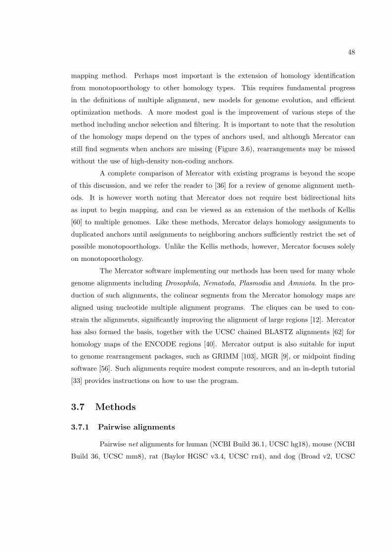
48

mapping method. Perhaps most important is the extension of homology identification

from monotopoorthology to other homology types. This requires fundamental progress

in the definitions of multiple alignment, new models for genome evolution, and efficient

optimization methods. A more modest goal is the improvement of various steps of the

method including anchor selection and filtering. It is important to note that the resolution

of the homology maps depend on the types of anchors used, and although Mercator can

still find segments when anchors are missing (Figure 3.6), rearrangements may be missed

without the use of high-density non-coding anchors.

A complete comparison of Mercator with existing programs is beyond the scope

of this discussion, and we refer the reader to [36] for a review of genome alignment meth-

ods. It is however worth noting that Mercator does not require best bidirectional hits

as input to begin mapping, and can be viewed as an extension of the methods of Kellis

[60] to multiple genomes. Like these methods, Mercator delays homology assignments to

duplicated anchors until assignments to neighboring anchors sufficiently restrict the set of

possible monotopoorthologs. Unlike the Kellis methods, however, Mercator focuses solely

on monotopoorthology.

The Mercator software implementing our methods has been used for many whole

genome alignments including Drosophila, Nematoda, Plasmodia and Amniota. In the pro-

duction of such alignments, the colinear segments from the Mercator homology maps are

aligned using nucleotide multiple alignment programs. The cliques can be used to con-

strain the alignments, significantly improving the alignment of large regions [12]. Mercator

has also formed the basis, together with the UCSC chained BLASTZ alignments [62] for

homology maps of the ENCODE regions [40]. Mercator output is also suitable for input

to genome rearrangement packages, such as GRIMM [103], MGR [9], or midpoint finding

software [56]. Such alignments require modest compute resources, and an in-depth tutorial

[33] provides instructions on how to use the program.

3.7 Methods

3.7.1 Pairwise alignments

Pairwise net alignments for human (NCBI Build 36.1, UCSC hg18), mouse (NCBI

Build 36, UCSC mm8), rat (Baylor HGSC v3.4, UCSC rn4), and dog (Broad v2, UCSC

49

Figure 3.6: Leveraging pairwise homology maps to build a multiple homology map. Theyellow regions indicate a set of monotopoorthologous segments in three genomes. The blue,red, and green colored rectangles are anchors, which fall into three pairwise cliques. Notethat no two genomes have more than one hit between them. However, in analyzing allthree genomes simultaneously, Mercator finds a run of these three cliques that contains twoanchors in each genome, which Mercator considers to be sufficient evidence for a mono-topoorthologous segment set.

canFam2) were obtained from the UCSC Genome Browser [59]. For each pair of genomes

(g1, g2), a one-to-one pairwise alignment was produced by taking the intersection of the

aligned nucleotide pairs in the corresponding g1-referenced and g2-referenced nets. Mercator

was then used to produce pairwise maps between the the four genomes. Coding exons from

all gene annotations available at the UCSC Genome Browser were extracted and a non-

overlapping set was selected for each genome as anchors. Hits were determined by running

BLAT [61] on the translated anchor sequences. Mercator was run with default parameters.

3.7.2 Consistency analysis

Human Ensembl gene annotations were obtained from UCSC for the NCBI Build

36 assembly. From a total of 433,669 coding exons in these annotations, a set of 201,473

non-overlapping exons was determined. The one-to-one pairwise alignments were then used

to map the exons from human to each of the other species. For those exon intervals that

had mappings to at least one other species, mappings of the mouse interval to rat, the dog

interval to mouse, and the rat interval to dog were also computed. It was then checked that

the two intervals computed for each species overlapped. If they did not, then the exon was

considered to have been mapped inconsistently by the pairwise alignments.

Mercator was used with the same anchor sets as for the pairwise maps to construct

a four-way map between the genomes. The 201,473 non-overlapping Ensembl coding exons

were part of the human anchor set, and were checked for being included in cliques in the

final Mercator output.

50

3.7.3 Comparative scaffolding

Pairwise chain alignments for human (NCBI Build 35, UCSC hg17), mouse (NCBI

Build 35, UCSC mm7), and rat (Baylor HGSC v3.1, UCSC rn3) were obtained from the

UCSC Genome Browser. A C++ program chainSegment (available in the Mercator dis-

tribution) was written to subdivide the chromosomes in each of the genomes into anchors,

using endpoints of the chains. Anchors were not allowed to overlap contig boundaries and

had a minimum length of 1kb (except in cases of contigs less than 1kb). After determining

a set of anchors, the chain alignments between two anchors were used by chainSegment

to assign scored hits. The coordinates of the anchors were transformed to be contig-based.

Mercator was run with default parameters on these anchors and hits and with all three

genomes specified as “draft”. The Mercator comparative scaffolding output was then com-

pared to the original AGP files (also obtained from UCSC) that describe the ordering of

the contigs within each of these assemblies.

51

Chapter 4

Parametric alignment of

Drosophila

The classic algorithms of Needleman–Wunsch and Smith–Waterman find a maxi-

mum a posteriori probability alignment for a pair hidden Markov model (PHMM). In order

to process large genomes that have undergone complex genome rearrangements, almost all

existing whole genome alignment methods apply fast heuristics to divide genomes into small

pieces which are suitable for Needleman–Wunsch alignment. In these alignment methods, it

is standard practice to fix the parameters and to produce a single alignment for subsequent

analysis by biologists.

As the number of alignment programs applied on a whole genome scale continues

to increase, so does the disagreement in their results. The alignments produced by different

programs vary greatly, especially in non-coding regions of eukaryotic genomes where the

biologically correct alignment is hard to find. Parametric alignment is one possible remedy.

This methodology resolves the issue of robustness to changes in parameters by finding all

optimal alignments for all possible parameters in a PHMM.

In this chapter we show that parametric sequence alignment can be made practi-

cal on the whole-genome scale. We demonstrate this through the construction of a whole

genome parametric alignment of Drosophila melanogaster and Drosophila pseudoobscura.

As described in Section 4.1, this alignment draws on existing heuristics for dividing whole

genomes into small pieces for alignment, and it relies on advances we have made in com-

puting convex polytopes that allow us to parametrically align non-coding regions using

52

biologically realistic models. We utilize the polytope construction algorithms introduced in

Section 2.1.6, which are based on the organizing principle of convexity, that was absent in

earlier studies [109, 48, 43].

Whole-genome parametric alignments can be very useful for comparative genomics

applications where reliable alignments are essential. We demonstrate the utility of our para-

metric alignment for biological inference by showing that cis-regulatory elements are more

conserved between Drosophila melanogaster and Drosophila pseudoobscura than previously

thought. We also show how whole genome parametric alignment can be used to quantita-

tively assess the dependence of branch length estimates on alignment parameters. Material

in this chapter previously appeared as part of the paper [34].

Alignment polytopes, software, and supplementary material can be downloaded at

http://bio.math.berkeley.edu/parametric/.

4.1 Whole-genome parametric alignment

The main computational result presented in this chapter is the construction of a

whole genome parametric alignment for two Drosophila genomes. This result depended on

a number of innovations. By adapting existing orthology mapping methods, we were able

to divide the genomes into 1,999,817 pairs of reliably orthologous segments, and among

these we identified 877,982 pairs for which the alignment is uncertain. We computed the

alignment polytopes of dimensions two, three and four for each of these 877,982 sequence

pairs, and of dimension five for a subset of them. The algorithms for the computation of

the polytopes are explained in Section 2.1.4. The vertices of these polytopes represent the

optimal alignment summaries and the robustness cones. These concepts were introduced in

Section 2.1.

4.1.1 Orthology mapping

The orthology mapping problem for a pair of genomes is to identify all orthologous

segments between the two genomes (Section 1.4.2). These orthologous segments, if selected

so as not to contain genome rearrangements, can then be globally aligned to each other.

This strategy is frequently used for whole-genome alignment [45, 110], and we adapted it for

our parametric alignment computation. For our alignment, we used the Mercator orthology

53

mapping program (Chapter 3) with the D. melanogaster and D. pseudoobscura genomes as

input to identify pieces for parametric alignment.

The Mercator orthology map for D. melanogaster and D. pseudoobscura has 2,731

segments. However, in order to obtain a map suitable for parametric alignment, further sub-

division of the segments was necessary. This subdivision was accomplished by the additional

step of identifying and fixing exact matches of length at least 10bp (see Section 4.5).

We derived 1,116,792 constraints, which are of four possible types:

• exact matching non-coding sequences,

• ungapped high scoring aligned coding sequences,

• segment pairs between two other constraints where one of the segments has length

zero, so the non-trivial segment must be gapped, and

• single nucleotide mismatches that are squeezed between other constraints.

We then removed all segments where the sequences contained the letter N (which means

the actual sequence is uncertain). This process resulted in 877,982 pairs of segments for

parametric alignment. The lengths of the D. melanogaster segments range from 1 to 80,676

base pairs. The median length is 42bp and the mean length is 99bp. In all, 90.4% of the

Drosophila melanogaster genome and 88.7% of the Drosophila pseudoobscura genome were

aligned by our method.

4.1.2 Polytope computation

The basic alignment model (Section 2.1.1) is insufficient for genomics applica-

tions. More realistic models for sequence alignment include gap penalties. Therefore, we

considered the three of the models defined in Section 2.1.3 in addition to the basic model

(d = 2). The symmetries of the scoring matrices for these models are derived from those of

the evolutionary models known as Jukes–Cantor (d = 3), Kimura-2 (d = 4) and Kimura-3

(d = 5).

We also considered two different methods for constructing all alignment polytopes

for the two Drosophila genomes: polytope propagation and incremental convex hull (Sec-

tion 2.1.6). In our study we found that polytope propagation was outperformed by the

incremental convex hull algorithm, especially for the higher dimensional models. Thus,

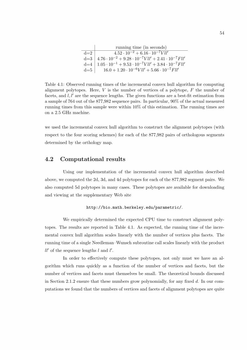
54

running time (in seconds)d=2 4.52 · 10−2 + 6.16 · 10−7V ll′

d=3 4.76 · 10−2 + 9.28 · 10−7V ll′ + 2.41 · 10−7Fll′

d=4 1.05 · 10−1 + 9.53 · 10−7V ll′ + 3.84 · 10−7Fll′

d=5 16.0 + 1.20 · 10−6V ll′ + 5.66 · 10−7Fll′

Table 4.1: Observed running times of the incremental convex hull algorithm for computingalignment polytopes. Here, V is the number of vertices of a polytope, F the number offacets, and l, l′ are the sequence lengths. The given functions are a best-fit estimation froma sample of 764 out of the 877,982 sequence pairs. In particular, 90% of the actual measuredrunning times from this sample were within 10% of this estimation. The running times areon a 2.5 GHz machine.

we used the incremental convex hull algorithm to construct the alignment polytopes (with

respect to the four scoring schemes) for each of the 877,982 pairs of orthologous segments

determined by the orthology map.

4.2 Computational results

Using our implementation of the incremental convex hull algorithm described

above, we computed the 2d, 3d, and 4d polytopes for each of the 877,982 segment pairs. We

also computed 5d polytopes in many cases. These polytopes are available for downloading

and viewing at the supplementary Web site

http://bio.math.berkeley.edu/parametric/.

We empirically determined the expected CPU time to construct alignment poly-

topes. The results are reported in Table 4.1. As expected, the running time of the incre-

mental convex hull algorithm scales linearly with the number of vertices plus facets. The

running time of a single Needleman–Wunsch subroutine call scales linearly with the product

ll′ of the sequence lengths l and l′.

In order to effectively compute these polytopes, not only must we have an al-

gorithm which runs quickly as a function of the number of vertices and facets, but the

number of vertices and facets must themselves be small. The theoretical bounds discussed

in Section 2.1.2 ensure that these numbers grow polynomially, for any fixed d. In our com-

putations we found that the numbers of vertices and facets of alignment polytopes are quite

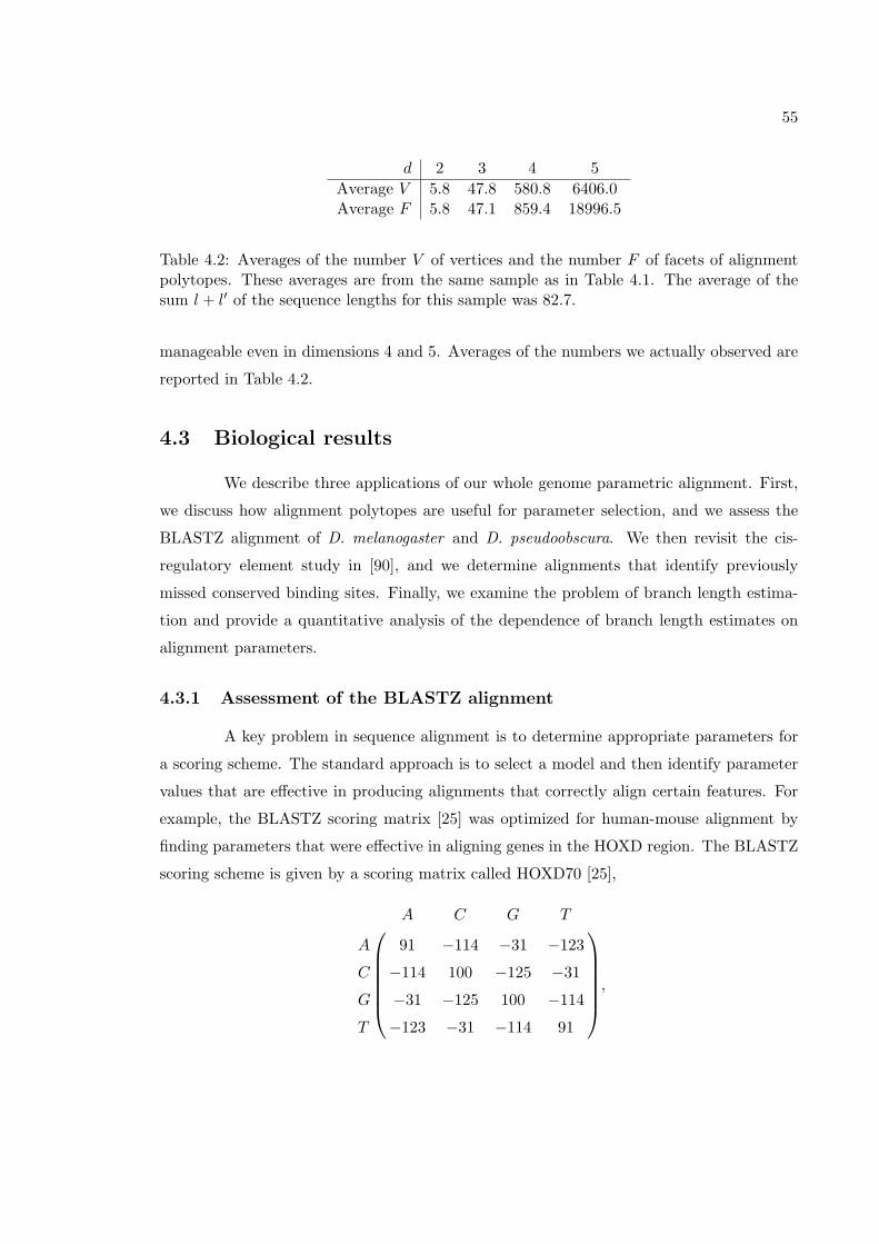
55

d 2 3 4 5Average V 5.8 47.8 580.8 6406.0Average F 5.8 47.1 859.4 18996.5

Table 4.2: Averages of the number V of vertices and the number F of facets of alignmentpolytopes. These averages are from the same sample as in Table 4.1. The average of thesum l + l′ of the sequence lengths for this sample was 82.7.

manageable even in dimensions 4 and 5. Averages of the numbers we actually observed are

reported in Table 4.2.

4.3 Biological results

We describe three applications of our whole genome parametric alignment. First,

we discuss how alignment polytopes are useful for parameter selection, and we assess the

BLASTZ alignment of D. melanogaster and D. pseudoobscura. We then revisit the cis-

regulatory element study in [90], and we determine alignments that identify previously

missed conserved binding sites. Finally, we examine the problem of branch length estima-

tion and provide a quantitative analysis of the dependence of branch length estimates on

alignment parameters.

4.3.1 Assessment of the BLASTZ alignment

A key problem in sequence alignment is to determine appropriate parameters for

a scoring scheme. The standard approach is to select a model and then identify parameter

values that are effective in producing alignments that correctly align certain features. For

example, the BLASTZ scoring matrix [25] was optimized for human-mouse alignment by

finding parameters that were effective in aligning genes in the HOXD region. The BLASTZ

scoring scheme is given by a scoring matrix called HOXD70 [25],

A C G T

A 91 −114 −31 −123

C −114 100 −125 −31

G −31 −125 100 −114

T −123 −31 −114 91

,

56

together with a space score of -30, and a gap score of -400. Although the HOXD70 matrix

has six distinct entries, it can be approximated by a Kimura-2 matrix (Table 2.2), since 91

is close to 100, and 114 is close to 123 and 125.

The alignment polytope of a pair of DNA sequences is a representation of all possi-

ble alignments organized according to a scoring scheme. Thus, our results and methodology

make it possible, for the first time, to identify parameters that are guaranteed to optimize

the alignment according to desired criteria. Moreover, our results offer biologists a math-

ematical tool for systematically assessing whether a proposed single alignment is suitable

for its intended purpose.

We initiated such a study for the BLASTZ [95] alignment of D. melanogaster

and D. pseudoobscura, which is available at http://genome.ucsc.edu/. This alignment is

widely used by biologists who study Drosophila. Although the BLASTZ alignment proce-

dure is based on an initial “seeding” procedure (similar to our identification of constrained

segment pairs), the alignments are then constructed using the Needleman–Wunsch algo-

rithm with the HOXD70 matrix.

Recall that our orthology map consisted of 1,999,817 segment pairs: 1,116,792

consisted of segments for which we fixed the alignment (constrained segment pairs) and

883,025 were unconstrained segment pairs for which we constructed alignment polytopes.

We found that the BLASTZ alignment agreed with 623,710 of our unconstrained segment

pairs, of which 622,173 did not contain Ns. For each of these 622,173 segment pairs, we

computed the 2d, 3d and 4d alignment summaries for the BLASTZ alignments, and we

determined whether or not they are optimal for some choice of model parameters.

We found that 269,186 (43.3%) of the BLASTZ alignments are vertices of the 3d

polytope, but not the 2d polytope, and 201,982 (32.5%) are vertices of both the 2d and

3d polytopes. Only 151,004 (24.3%) of the BLASTZ alignments are not vertices of either

the 2d or 3d alignment polytopes. In summary, our computations show that 32.5% of the

BLASTZ alignments correspond to vertices of the 2d polytope and 75.7% correspond to

vertices of the 3d polytope. These numbers are even higher for the 4d and 5d polytopes.

Curiously, there is precisely one sequence pair where the BLASTZ alignment is a

vertex of the 2d polytope but not the 3d polytope. This alignment is

mel AGCCGAACCGGATATCCAGGCCGAGGCCpse GCCAGAGCCGGA-GCCTGAGCCGGAG--

* ** ***** * *** *

57

The 3d summary of this alignment is (11, 3, 2), which is the midpoint of the edge

with vertices (11, 3, 1) and (11, 3, 3) on the 3d polytope. Hence this alignment is not optimal

for any choice of parameters (X,S,G). However, it is optimal for the 2d model since the

edge maps onto the vertex (11, 3) of the 2d polygon.

Our results show that not only does the BLASTZ alignment agree well with our

constrained segment pairs, but, even on the unconstrained segment pairs, the BLASTZ

alignments are mostly vertices of the three dimensional polytopes. This suggests that there

may be a statistical advantage to working with one of the lower dimensional models, and

also indicates that the polytopes may be useful for finding parameters. We illustrate this

point of view in the next section, where we identify vertices in the alignment polytope (and

therefore parameter robustness cones) that are suitable for the alignment of cis-regulatory

elements. Any user of the BLASTZ alignments may now use the alignment polytopes we

provide in order to assess whether or not the fixed choice of the HOXD70 matrix is the

right one for their particular biological application.

4.3.2 Conservation of cis-regulatory elements

A central question in comparative genomics is the extent of conservation of cis-

regulatory elements, and the implications for genome function and evolution. Using our

parametric alignment, we discovered that cis-regulatory elements may be more conserved

between D. melanogaster and D. pseudoobscura than previously thought. Specifically, we

used our alignment polytopes to examine the degree of conservation for 1346 transcription

factor binding sites [4] available at http://www.flyreg.org (we excluded 16 sites which

were located in segment pairs containing Ns). The 1346 sites include the 142 sites examined

by Richards et al. [90] in their comparison of D. pseudoobscura and D. melanogaster.

Specifically, for each of the 1346 elements, we identified the orthologous segment

pairs from our orthology map that contained the elements. We then extracted the poly-

topes from our whole genome parametric alignment. For each polytope, we determined an

optimal alignment for which the number of matching bases of the corresponding element

was maximized.

As an example consider the transcription factor Adf1. It binds to a cis-regulatory

element at chr3R:2,825,118-2,825,144 in D. melanogaster (Adf1-> Antp:06447 in the flyreg

58

database). The BLASTZ alignment for this element is

mel TGTGCGTCAGCGTCGGCCGCAACAGCGpse TGT-----------------GACTGCG

*** ** ***

This alignment suggests that the D. melanogaster cis-regulatory element is not conserved

in D. pseudoobscura. However, there are many optimal alignments which indicate that this

element is conserved. Examining our constrained segment pairs, we found that the prefix

TGTG was at the end of a 13bp exact match. The remaining D. melanogaster element was

part of a segment pair which has 813 distinct optimal alignments in the 3d model. Among

these, we found the following alignment with parameters G = −3, S = −8, X = −18:

mel TGTG----CGTCAGC--G----TCGGCC---GC-AACAG-CGpse TGTGACTGCG-CTGCCTGGTCCTCGGCCACAGCCAAC-GTCG

**** ** * ** * ****** ** *** * **

Note that we include the TGTG prefix in order to show a complete alignment of the cis-

regulatory element. The second alignment has 24 matches instead of the BLASTZ alignment

with 8. The number of matches can be used to calculate the percent identity for an element

as follows:

percent identity = 100× #matches#bases in element

.

Percent identity was used in [90] as a criterion for determine whether binding sites are

conserved. The BLASTZ alignment has 30% identity and the alignment with 24 matches

has 89% identity. It is an optimal alignment with the highest possible percent identity.

Examining all 813 optimal alignments, it appeared to us that the following alignment (ob-

tained with G = −882, S = −87, X = −226) is more reasonable, even though it has a lower

percent identity (67%):

mel TGTGCGTCAGC------GTCGGCCGCAACAGCGpse TGTGACTGCGCTGCCTGGTCCTCGGCCACAGC-

**** * ** *** * ** *****

This alternative alignment suggests that the percent identity criterion may not be the best

way to judge the conservation of elements. Regardless, we believe our parametric alignment

indicates that in this particular case, the D. melanogaster cis-regulatory element is likely

to have been conserved in D. pseudoobscura.

Our overall results are summarized in Table 4.3. We found that parameters can

be chosen so as to significantly increase the number of matches for cis-regulatory elements.

59

2d 3d 4d

Mean % id opt param 80.4 85.1 86.5

Mean % id fix param 79.1 − −

Table 4.3: Cis-regulatory element conservation.

The “opt param” row in the table shows results for the case where parameters were chosen

separately for each segment pair so as to maximize the % identity of the cis-regulatory

elements. The “fix param” row shows results when one parameter was selected (optimally)

for all segment pairs simultaneously (this was only computed for the 2d model). Note that

the mean per site % identity reported in [90] was 51.3%, considerably lower than what we

found using the whole genome parametric alignment (even for the 2d model).

Our results seem to indicate that cis-regulatory elements are more conserved be-

tween D. melanogaster and D. pseudoobscura than previously thought. The alignment

polytopes should be a useful tool for further investigation of the extent of conservation of

cis-regulatory elements among the Drosophila genomes.

4.3.3 The Jukes–Cantor distance function

An important problem in molecular evolution is the estimation of branch lengths

from aligned genome sequences. A widely used method for estimating branch lengths is

based on the Jukes–Cantor model of evolution [57]. Given an alignment of two sequences

of lengths l, l′, with 2d alignment summary (x, s), one computes the Jukes–Cantor distance

of the two genomes as follows:

dJC(x, s) = −34log

(1− 4

3

(2x

l + l′ − s

)).

See [83, Proposition 4.6] for a derivation of this expression which is also known as the

Jukes–Cantor correction of the two aligned sequences. The Jukes–Cantor distance can be

interpreted as the expected number of mutations per site.

Since the Jukes–Cantor distance dJC(x, s) depends on the underlying pairwise

sequence alignment summary, which in turn depends on the alignment parameters, it is

natural to ask how the branch length estimate depends on the parameters in a 2d scoring

scheme. We therefore introduce the Jukes–Cantor distance function which is the function

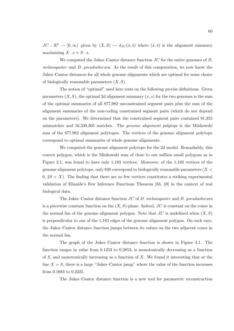
60

JC : R2 → [0,∞) given by (X,S) 7→ dJC(x, s) where (x, s) is the alignment summary

maximizing X · x+ S · s.We computed the Jukes–Cantor distance function JC for the entire genomes of D.

melanogaster and D. pseudoobscura. As the result of this computation, we now know the

Jukes–Cantor distances for all whole genome alignments which are optimal for some choice

of biologically reasonable parameters (X,S).

The notion of “optimal” used here rests on the following precise definitions. Given

parameters (X,S), the optimal 2d alignment summary (x, s) for the two genomes is the sum

of the optimal summaries of all 877,982 unconstrained segment pairs plus the sum of the

alignment summaries of the non-coding constrained segment pairs (which do not depend

on the parameters). We determined that the constrained segment pairs contained 91,355

mismatches and 16,339,305 matches. The genome alignment polytope is the Minkowski

sum of the 877,982 alignment polytopes. The vertices of the genome alignment polytope

correspond to optimal summaries of whole genome alignments.

We computed the genome alignment polytope for the 2d model. Remarkably, this

convex polygon, which is the Minkowski sum of close to one million small polygons as in

Figure 2.1, was found to have only 1,183 vertices. Moreover, of the 1,183 vertices of the

genome alignment polytope, only 838 correspond to biologically reasonable parameters (X <

0, 2S < X). The finding that there are so few vertices constitutes a striking experimental

validation of Elizalde’s Few Inference Functions Theorem [83, §9] in the context of real

biological data.

The Jukes–Cantor distance function JC of D. melanogaster and D. pseudoobscura

is a piecewise constant function on the (X,S)-plane. Indeed, JC is constant on the cones in

the normal fan of the genome alignment polygon. Note that JC is undefined when (X,S)

is perpendicular to one of the 1,183 edges of the genome alignment polygon. On such rays,

the Jukes–Cantor distance function jumps between its values on the two adjacent cones in

the normal fan.

The graph of the Jukes–Cantor distance function is shown in Figure 4.1. The

function ranges in value from 0.1253 to 0.2853, is monotonically decreasing as a function

of S, and monotonically increasing as a function of X. We found it interesting that at the

line X = S, there is a large “Jukes–Cantor jump” where the value of the function increases

from 0.1683 to 0.2225.

The Jukes–Cantor distance function is a new tool for parametric reconstruction

61

−300−250

−200−150

−100−50

0

−300−250

−200−150

−100−50

0

0

0.05

0.1

0.15

0.2

0.25

0.3

0.35

XS

JC(X,S)

Figure 4.1: The Jukes–Cantor distance function of two Drosophila genomes.

of phylogenetic trees. Instead of estimating a single distance between each pair of genomes

in a multiple species phylogenetic reconstruction, one can now evaluate the Jukes–Cantor

function at vertices of the Minkowski sum of the whole genome alignment polytopes. These

can be used for parametric phylogenetic reconstruction using distance-based methods such

as neighbor joining.

4.4 Discussion

The summary of a pair of aligned sequences is a list of numbers that determine

the score for a scoring scheme. The alignment polytope is a geometric representation of

the summaries of all alignments. It is an organizing tool for working with all alignments

through their summaries. We view the Needleman–Wunsch algorithm as a fast subroutine

for finding vertices of the alignment polytope. The construction of alignment polytopes is

useful for biological studies based on sequence alignments where the conclusions depend on

parameter choices.

We have highlighted three biological applications of our parametric alignments,

62

namely the problem of parameter selection for sequence alignment, functional element con-

servation, and estimation of evolutionary rate parameters. In each case, our perspective

suggests new directions for further research.

Alignment polytopes offer a systematic approach to solving the parameter selection

problem. Although this chapter did not address statistical aspects of parameter selection,

we wish to emphasize that the vertices of the polytopes represent maximum a posteriori

estimates of alignments for pair hidden Markov models. Our polytopes provide a setting

for developing statistically sound methods for parameter selection that are not dependent

on pre-existing alignments.

Our results on cis-regulatory elements show that they may be significantly more

conserved than previously thought, and suggest that, in contrast to the analysis of ultra-

conserved elements, sequence alignment procedures can be crucial in the analysis of certain

functional elements. The ongoing Drosophila genome projects (consisting of sequencing 12

genomes of related species) offer an extraordinary opportunity for extending our study and

further exploring cis-regulatory element conservation. This leads to the question of multiple

alignment, which we have not addressed in this chapter, but which we believe presents a

formidable and important challenge in biological sequence analysis. In particular, it will

be interesting to explore the geometric point of view we have proposed and to develop

parametric algorithms for multiple sequence alignment.

The Jukes–Cantor distance function, computed here for the first time, will be

important for determining the robustness of evolutionary studies based on sequence align-

ments. Estimates of the neutral rate of evolution, which are crucial for comparative ge-

nomics studies, can hopefully be improved and further developed using our mathematical

tools. The Jukes–Cantor distance function opens up the possibility of parametric distance-

based phylogenetic reconstruction. An immediate next step is the extension of our results

to other phylogenetic models.

The construction of millions of alignment polytopes from two Drosophila genomes

has revealed mathematical insights that should be explored further. For example, we ob-

served empirically that alignment polytopes have few facets. Although we have not explored

the combinatorial structure of alignment polytopes in this chapter, this offers a promising

direction for improving our parametric alignment algorithms and is an interesting direction

for future research.

63

4.5 Methods

The data analyzed are the genome sequences of Drosophila melanogaster (April

2004 BDGP release 4) and Drosophila pseudoobscura (August 2003 freeze 1).

Gene annotations for identifying exons were based on reference gene sets and ab

initio predictions. For Drosophila melanogaster we used Flybase [37], SNAP, genscan,

geneid and RefSeq. Twinscan, SNAP, genscan, geneid and xenoRefSeq (mRNAs from other

species) were used for Drosophila pseudoobscura. Annotations were obtained from the UCSC

genome browser, except for SNAP which we ran ourselves.

MUMmer v3.18 [32] was used to obtain potential non-coding anchors (20bp exact

matches). MUMmer was also run on orthologous segments determined by Mercator to

identify ≥ 10bp exact matches to refine the orthology map.

The Beneath-Beyond and polytope propagation algorithms were implemented in

C++. Source code and binaries are available at the supplementary web site.

The BLASTZ alignment was obtained from the UCSC genome browser. The “net”

and “chain” tracks were used to determine the best alignment for each interval in Drosophila

melanogaster. The resulting alignment blocks were compared to our constraints.

The transcription factor binding sites used in the cis-regulatory element study

were obtained at http://www.flyreg.org. 16 sites were excluded because of segment

pairs containing Ns.

Computations were carried out on an 18 node (36-CPU at 2.3GhZ each) cluster.

Each node had 2GB RAM.

64

Chapter 5

Parametric phylogeny

In Chapter 4, we showed how parametric alignment methods could be used on

pairs of genomic sequences to aid in biological inference. This chapter explores the use

of parametric methods in the case of multiple sequences. The Minkowski sum of pairwise

alignment polytopes is shown to be perfectly suited to analyzing the guide-tree construction

methods of CLUSTAL W, a popular multiple alignment program. Utilizing the statistical

alignment model discussed in Section 2.2, we additionally show how to assign posterior

probabilities to polytope vertices and, in our application, to guide-tree topologies. An

intron sequence from four Drosophila species is used as an example application.

5.1 Phylogeny in CLUSTAL W

CLUSTAL W [104] has been one of the most widely used multiple alignment

programs in the field of computational biology. The program has the following steps.

1. Alignments of all pairs of input sequences are computed. This is done either by

the Needleman–Wunsch algorithm, or by a faster heuristic method. A single set of

parameter values is used for all alignments.

2. The pairwise alignments are used to determine a distance matrix. The distance be-

tween two sequences is calculated as xm+x , where m and x are the number of matches

and mismatches in the pairwise alignment, respectively. Thus, distances do not take

into account gaps and are not corrected for multiple substitutions (e.g., using the

Jukes–Cantor correction, Section 4.3.3).

65

3. A phylogenetic tree is determined from the distance matrix using the Neighbor-Joining

algorithm [91].

4. The sequences are put into a multiple alignment using a progressive method, which

uses the tree computed in the previous step as a guide.

The guide-tree used by progressive methods plays a major role in shaping the final multiple

alignments. In the case of CLUSTAL W, the parameter values used in the first alignment

step could greatly impact this guide tree. To explore the dependence of the guide-tree on

the initial alignment parameters, we undertook a parametric analysis of the first three steps

of CLUSTAL W. The following two sections explain the methods required for this analysis.

5.2 Pairwise distances from alignment polytopes

We take the approach used in Section 4.3.3 to organize sets of optimal pairwise

alignments between multiple input sequences. Given n input sequences, we can compute

all(n2

)pairwise alignment polytopes. The Minkowski sum of these polytopes represents the

possible combinations of these pairwise alignments. Specifically, each vertex of this larger

polytope is the sum of(n2

)pairwise alignment summaries, one from each of the pairwise

polytopes. The pairwise alignment summaries contained in this set are simultaneously

optimal for some parameter values (those contained within the normal cone of the Minkowski

sum vertex). Because a distance can be calculated from each pairwise alignment, the vertices

of the Minkowski sum polytope also represent distance matrices.

5.3 Assigning posterior probabilities to polytope vertices

By taking advantage of the correspondence between the statistical alignment model

described in Section 2.2 and the classic Needleman–Wunsch algorithm, we can enhance the

output of our parametric alignment method. Recall that an alignment polytope has all

possible optimal alignment summaries as its vertices. Although it is informative to have

such a set of summaries, one might like to say that certain summaries are more reasonable

than others, given the data and prior beliefs, with respect to the parameters that make

them optimal. The PHMM from Section 2.2 and Bayesian statistics allow us to make

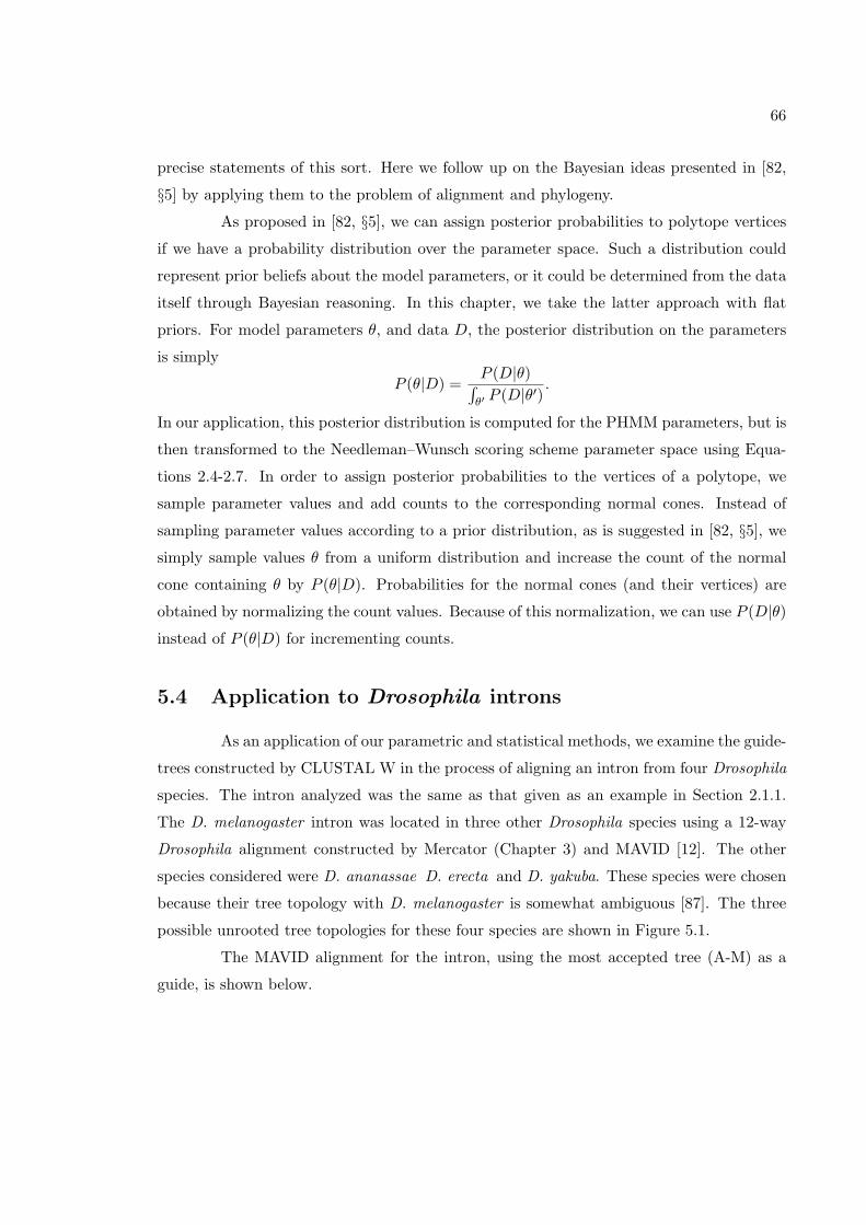
66

precise statements of this sort. Here we follow up on the Bayesian ideas presented in [82,

§5] by applying them to the problem of alignment and phylogeny.

As proposed in [82, §5], we can assign posterior probabilities to polytope vertices

if we have a probability distribution over the parameter space. Such a distribution could

represent prior beliefs about the model parameters, or it could be determined from the data

itself through Bayesian reasoning. In this chapter, we take the latter approach with flat

priors. For model parameters θ, and data D, the posterior distribution on the parameters

is simply

P (θ|D) =P (D|θ)∫

θ′ P (D|θ′).

In our application, this posterior distribution is computed for the PHMM parameters, but is

then transformed to the Needleman–Wunsch scoring scheme parameter space using Equa-

tions 2.4-2.7. In order to assign posterior probabilities to the vertices of a polytope, we

sample parameter values and add counts to the corresponding normal cones. Instead of

sampling parameter values according to a prior distribution, as is suggested in [82, §5], we

simply sample values θ from a uniform distribution and increase the count of the normal

cone containing θ by P (θ|D). Probabilities for the normal cones (and their vertices) are

obtained by normalizing the count values. Because of this normalization, we can use P (D|θ)instead of P (θ|D) for incrementing counts.

5.4 Application to Drosophila introns

As an application of our parametric and statistical methods, we examine the guide-

trees constructed by CLUSTAL W in the process of aligning an intron from four Drosophila

species. The intron analyzed was the same as that given as an example in Section 2.1.1.

The D. melanogaster intron was located in three other Drosophila species using a 12-way

Drosophila alignment constructed by Mercator (Chapter 3) and MAVID [12]. The other

species considered were D. ananassae D. erecta and D. yakuba. These species were chosen

because their tree topology with D. melanogaster is somewhat ambiguous [87]. The three

possible unrooted tree topologies for these four species are shown in Figure 5.1.

The MAVID alignment for the intron, using the most accepted tree (A-M) as a

guide, is shown below.

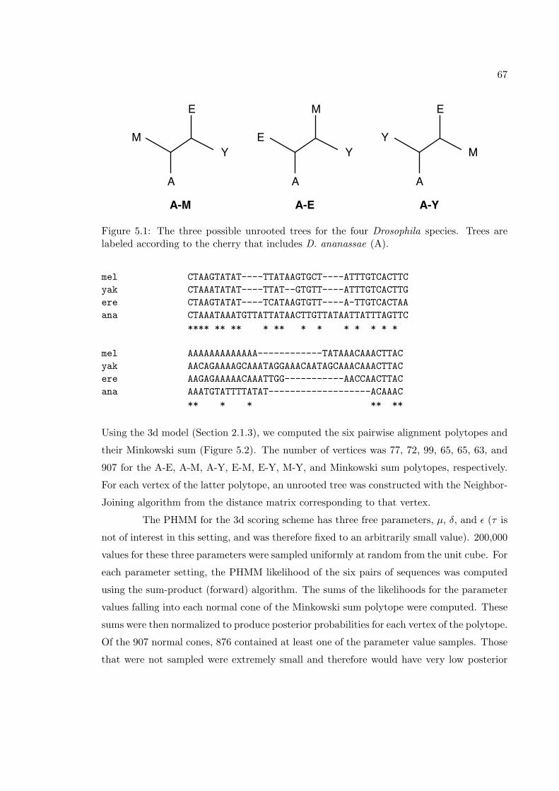
67

M

A

E

YE

A

M

YY

A

E

M

A-M A-E A-Y

Figure 5.1: The three possible unrooted trees for the four Drosophila species. Trees arelabeled according to the cherry that includes D. ananassae (A).

mel CTAAGTATAT----TTATAAGTGCT----ATTTGTCACTTCyak CTAAATATAT----TTAT--GTGTT----ATTTGTCACTTGere CTAAGTATAT----TCATAAGTGTT----A-TTGTCACTAAana CTAAATAAATGTTATTATAACTTGTTATAATTATTTAGTTC

**** ** ** * ** * * * * * * *

mel AAAAAAAAAAAAA------------TATAAACAAACTTACyak AACAGAAAAGCAAATAGGAAACAATAGCAAACAAACTTACere AAGAGAAAAACAAATTGG-----------AACCAACTTACana AAATGTATTTTATAT-------------------ACAAAC

** * * ** **

Using the 3d model (Section 2.1.3), we computed the six pairwise alignment polytopes and

their Minkowski sum (Figure 5.2). The number of vertices was 77, 72, 99, 65, 65, 63, and

907 for the A-E, A-M, A-Y, E-M, E-Y, M-Y, and Minkowski sum polytopes, respectively.

For each vertex of the latter polytope, an unrooted tree was constructed with the Neighbor-

Joining algorithm from the distance matrix corresponding to that vertex.

The PHMM for the 3d scoring scheme has three free parameters, µ, δ, and ε (τ is

not of interest in this setting, and was therefore fixed to an arbitrarily small value). 200,000

values for these three parameters were sampled uniformly at random from the unit cube. For

each parameter setting, the PHMM likelihood of the six pairs of sequences was computed

using the sum-product (forward) algorithm. The sums of the likelihoods for the parameter

values falling into each normal cone of the Minkowski sum polytope were computed. These

sums were then normalized to produce posterior probabilities for each vertex of the polytope.

Of the 907 normal cones, 876 contained at least one of the parameter value samples. Those

that were not sampled were extremely small and therefore would have very low posterior

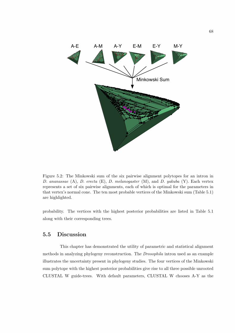
68

A-E A-M A-Y E-M E-Y M-Y

Minkowski Sum

Figure 5.2: The Minkowski sum of the six pairwise alignment polytopes for an intron inD. ananassae (A), D. erecta (E), D. melanogaster (M), and D. yakuba (Y). Each vertexrepresents a set of six pairwise alignments, each of which is optimal for the parameters inthat vertex’s normal cone. The ten most probable vertices of the Minkowski sum (Table 5.1)are highlighted.

probability. The vertices with the highest posterior probabilities are listed in Table 5.1

along with their corresponding trees.

5.5 Discussion

This chapter has demonstrated the utility of parametric and statistical alignment

methods in analyzing phylogeny reconstruction. The Drosophila intron used as an example

illustrates the uncertainty present in phylogeny studies. The four vertices of the Minkowski

sum polytope with the highest posterior probabilities give rise to all three possible unrooted

CLUSTAL W guide-trees. With default parameters, CLUSTAL W chooses A-Y as the

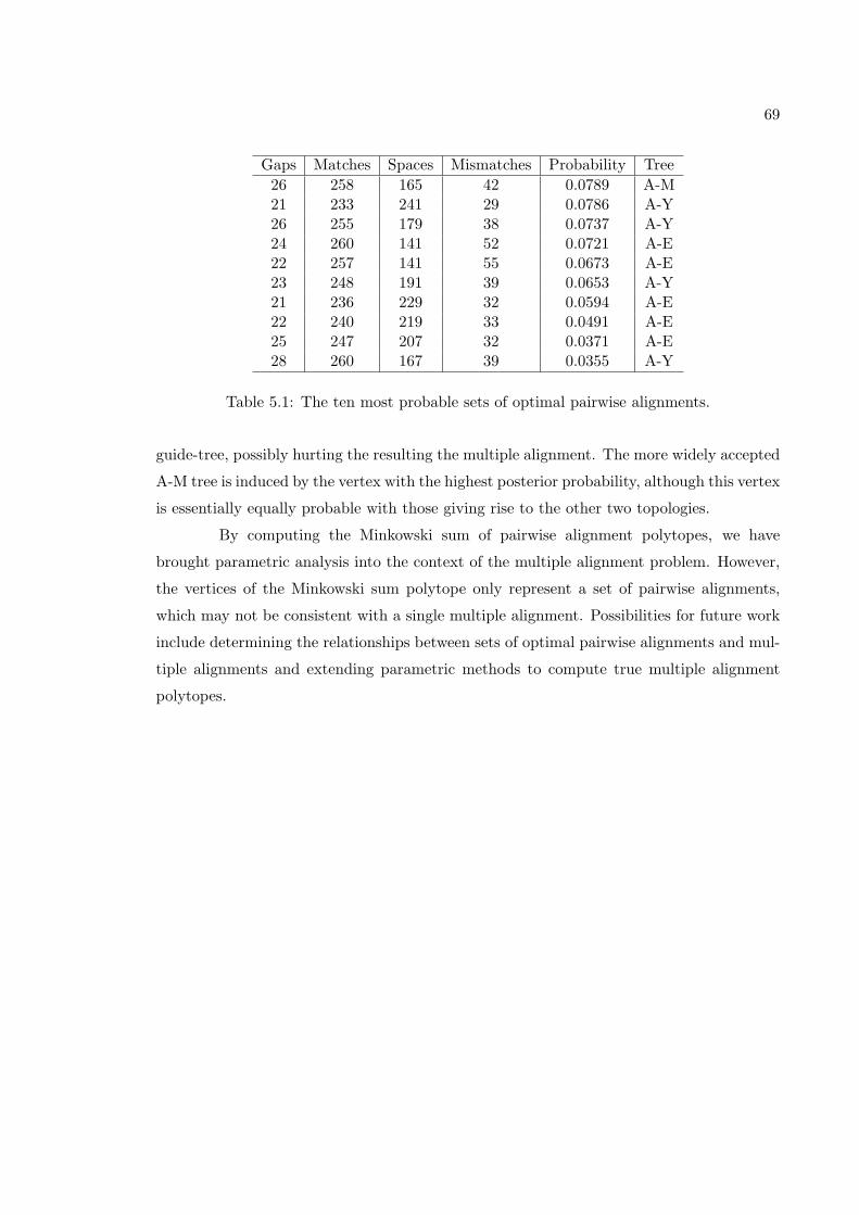
69

Gaps Matches Spaces Mismatches Probability Tree26 258 165 42 0.0789 A-M21 233 241 29 0.0786 A-Y26 255 179 38 0.0737 A-Y24 260 141 52 0.0721 A-E22 257 141 55 0.0673 A-E23 248 191 39 0.0653 A-Y21 236 229 32 0.0594 A-E22 240 219 33 0.0491 A-E25 247 207 32 0.0371 A-E28 260 167 39 0.0355 A-Y

Table 5.1: The ten most probable sets of optimal pairwise alignments.

guide-tree, possibly hurting the resulting the multiple alignment. The more widely accepted

A-M tree is induced by the vertex with the highest posterior probability, although this vertex

is essentially equally probable with those giving rise to the other two topologies.

By computing the Minkowski sum of pairwise alignment polytopes, we have

brought parametric analysis into the context of the multiple alignment problem. However,

the vertices of the Minkowski sum polytope only represent a set of pairwise alignments,

which may not be consistent with a single multiple alignment. Possibilities for future work

include determining the relationships between sets of optimal pairwise alignments and mul-

tiple alignments and extending parametric methods to compute true multiple alignment

polytopes.

70

Bibliography

[1] S F Altschul, W Gish, W Miller, E W Myers, and D J Lipman. Basic local alignment

search tool. J. Mol. Biol., 215:403–410, 1990.

[2] Serafim Batzoglou. The many faces of sequence alignment. Brief. Bioinform., 6:6–22,

2005.

[3] G Benson. Tandem repeats finder: a program to analyze DNA sequences. Nucleic

Acids Res., 27(2):573–580, 1999.

[4] Casey M Bergman, Joseph W Carlson, and Susan E Celniker. Drosophila dnase i

footprint database: a systematic genome annotation of transcription factor binding

sites in the fruitfly, drosophila melanogaster. Bioinformatics, 21(1367-4803):1747–9,

2005.

[5] E Birney, D Andrews, M Caccamo, Y Chen, L Clarke, G Coates, T Cox, F Cun-

ningham, V Curwen, T Cutts, et al. Ensembl 2006. Nucleic Acids Res., 34(Database

issue):D556–61, Jan 2006.

[6] Jaime E Blair, Prachi Shah, and S Blair Hedges. Evolutionary sequence analysis of

complete eukaryote genomes. BMC Bioinformatics, 6:53, 2005.

[7] M Blanchette, ED Green, W Miller, and D Haussler. Reconstructing large regions of

an ancestral mammalian genome in silico. Genome Res., 14(12):2412–2423, Dec 2004.

[8] M Blanchette, WJ Kent, C Riemer, L Elnitski, AF Smit, KM Roskin, R Baertsch,

K Rosenbloom, H Clawson, ED Green, et al. Aligning multiple genomic sequences

with the threaded blockset aligner. Genome Res., 14(4):708–715, Apr 2004.

71

[9] G Bourque and PA Pevzner. Genome-scale evolution: reconstructing gene orders in

the ancestral species. Genome Res., 12(1):26–36, Jan 2002.

[10] G Bourque, PA Pevzner, and G Tesler. Reconstructing the genomic architecture of

ancestral mammals: lessons from human, mouse, and rat genomes. Genome Res.,

14(4):507–516, Apr 2004.

[11] N Bray, I Dubchak, and L Pachter. Avid: A global alignment program. Genome Res.,

13(1):97–102, Jan 2003.

[12] Nicolas Bray and Lior Pachter. MAVID: Constrained ancestral alignment of multiple

sequences. Genome Res., 14(4):693–699, 2004.

[13] T A Brown. Genomes. John Wiley & Sons, Inc., New York, NY, 1999.

[14] M Brudno, M Chapman, B Gottgens, S Batzoglou, and B Morgenstern. Fast and

sensitive multiple alignment of large genomic sequences. BMC Bioinformatics, 4:66,

Dec 2003.

[15] M Brudno, CB Do, GM Cooper, MF Kim, E Davydov, ED Green, A Sidow, and S Bat-

zoglou. LAGAN and Multi-LAGAN: efficient tools for large-scale multiple alignment

of genomic DNA. Genome Res., 13(4):721–731, Apr 2003.

[16] M Brudno, A Poliakov, A Salamov, GM Cooper, A Sidow, EM Rubin, V Solovyev,

S Batzoglou, and I Dubchak. Automated whole-genome multiple alignment of rat,

mouse, and human. Genome Res., 14(4):685–692, Apr 2004.

[17] C Burge and S Karlin. Prediction of complete gene structures in human genomic

DNA. J. Mol. Biol., 268(1):78–94, 1997.

[18] Peter P Calabrese, Sugata Chakravarty, and Todd J Vision. Fast identification and

statistical evaluation of segmental homologies in comparative maps. Bioinformatics,

19 Suppl 1:i74–80, 2003.

[19] SB Cannon and ND Young. OrthoParaMap: distinguishing orthologs from paralogs

by integrating comparative genome data and gene phylogenies. BMC Bioinformatics,

4:35, Sep 2003.

72

[20] Steven B Cannon, Alexander Kozik, Brian Chan, Richard Michelmore, and Nevin D

Young. DiagHunter and GenoPix2D: programs for genomic comparisons, large-scale

homology discovery and visualization. Genome Biol., 4:R68, 2003.

[21] Anat Caspi. Homology mapping with markov random fields. In Pachter and Sturmfels

[83], pages 264–277.

[22] K Chakrabarti and L Pachter. Visualization of multiple genome annotations and

alignments with the K-BROWSER. Genome Res., 14(4):716–20, Apr 2004.

[23] H L Chan, T W Lam, W K Sung, Prudence W H Wong, S M Yiu, and X Fan.

The mutated subsequence problem and locating conserved genes. Bioinformatics,

21:2271–8, 2005.

[24] Xin Chen, Jie Zheng, Zheng Fu, Peng Nan, Yang Zhong, Stefano Lonardi, and Tao

Jiang. Assignment of orthologous genes via genome rearrangement. IEEE/ACM

Trans. Comput. Biol. Bioinformatics, 2(4):302–315, 2005.

[25] F Chiaromonte, V B Yap, and W Miller. Scoring pairwise genomic sequence align-

ments. Pac Symp Biocomput, pages 115–26, 2002.

[26] A Clark, G Gibson, T Kaufman, B McAllister, G Myers, and P O’Grady. Drosophila

as a model system for comparative genomics. White Paper to NHGRI, June 2003.

[27] GM Cooper, EA Stone, G Asimenos, ED Green, S Batzoglou, and A Sidow. Distri-

bution and intensity of constraint in mammalian genomic sequence. Genome Res.,

15(7):901–913, Jul 2005.

[28] Olivier Couronne, Alexander Poliakov, Nicolas Bray, Tigran Ishkhanov, Dmitriy

Ryaboy, Edward Rubin, Lior Pachter, and Inna Dubchak. Strategies and Tools for

Whole-Genome Alignments. Genome Res., 13(1):73–80, 2003.

[29] Val Curwen, Eduardo Eyras, T. Daniel Andrews, Laura Clarke, Emmanuel Mongin,

Steven M. J. Searle, and Michele Clamp. The ensembl automatic gene annotation

system. Genome Res., 14(5):942–950, 2004.

[30] Aaron C E Darling, Bob Mau, Frederick R Blattner, and Nicole T Perna. Mauve:

multiple alignment of conserved genomic sequence with rearrangements. Genome

Res., 14(7):1394–403, 2004.

73

[31] Aaron E Darling, Bob Mau, Frederick R Blattner, and Nicole T Perna. GRIL: genome

rearrangement and inversion locator. Bioinformatics, 20(1):122–124, 2004.

[32] AL Delcher, S Kasif, RD Fleischmann, J Peterson, O White, and AL Salzberg. Align-

ment of whole genomes. Nucleic Acids Res., 27:2369–2376, 1999.

[33] Colin N Dewey. Aligning multiple whole genomes with Mercator and MAVID. To

appear in the Comparative Genomics volume of the Methods in Molecular Biology

series, Humana Press, 2006.

[34] Colin N. Dewey, Peter M. Huggins, Kevin Woods, Bernd Sturmfels, and Lior Pachter.

Parametric alignment of Drosophila genomes. PLoS Computational Biology, 2(6):e73,

2006.

[35] Colin N Dewey and Lior Pachter. Mercator: multiple whole-genome orthology map

construction. In preparation.

[36] Colin N Dewey and Lior Pachter. Evolution at the nucleotide level: the problem of

multiple whole-genome alignment. Hum. Mol. Genet., 15:R51–R56, 2006.

[37] RA Drysdale, MA Crosby, and The Flybase Consortium. Flybase: Genes and gene

models. Nucleic Acids Res., 33:D390–D395, 2005.

[38] R Durbin, S Eddy, A Korgh, and G Mitchison. Biological Sequence Analysis: Proba-

bilistic Models of Proteins and Nucleic Acids. Cambridge University Press, 1998.

[39] Jonathan Eisen and Claire M Fraser. Phylogenomics: Intersection of evolution and

genomics. Science, 300(5626):1706–1707, 2003.

[40] ENCODE Project Consortium. The ENCODE (ENCyclopedia Of DNA Elements)

Project. Science, 306:636–40, 2004.

[41] J Felsenstein. Inferring Phylogenies. Sinauer Associates, Inc., Sunderland, Mass,

2003.

[42] D Fernandez-Baca, T Seppalainen, and G Slutzki. Parametric multiple sequence

alignment and phylogeny construction. Journal of Discrete Algorithms, 2(2):271–287,

2004.

74

[43] D Fernandez-Baca and B Venkatachalam. Parametric sequence alignment. In S Aluru,

editor, Handbook of Computational Molecular Biology, volume 2, pages 271–287.

Chapman and Hall/CRC Press Computer and Information Science Series, 2005.

[44] W M Fitch. Homology a personal view on some of the problems. Trends Genet.,

16(5):227–231, 2000.

[45] Richard A Gibbs, George M Weinstock, Michael L Metzker, Donna M Muzny, Erica J

Sodergren, Steven Scherer, Graham Scott, David Steffen, Kim C Worley, Paula E

Burch, et al. Genome sequence of the brown norway rat yields insights into mammalian

evolution. Nature, 428:493–521, 2004.

[46] B Grunbaum. Convex Polytopes, volume 221 of Graduate Texts in Mathematics.

Springer-Verlag, New York, second edition, 2003. Prepared and with a preface by

Volker Kaibel, Victor Klee and Gunter M. Ziegler.

[47] R Guigo. Assembling genes from predicted exons in linear time with dynamic pro-

gramming. J. Comput. Biol., 5(4):681–702, 1998.

[48] D Gusfield, K Balasubramanian, and D Naor. Parametric optimization of sequence

alignment. Algorithmica, 12:312–326, 1994.

[49] D Gusfield and P Stelling. Parametric and inverse-parametric sequence alignment

with XPARAL. Methods Enzymology, 266:481–494, 1996.

[50] Brian J Haas, Arthur L Delcher, Jennifer R Wortman, and Steven L Salzberg.

DAGchainer: a tool for mining segmental genome duplications and synteny. Bioin-

formatics, 20:3643–6, 2004.

[51] Brian K Hall, editor. Homology: the hierarchical basis of comparative biology. Aca-

demic Press, Inc., San Diego, CA, 1994.

[52] S E Hampson, B S Gaut, and P Baldi. Statistical detection of chromosomal homology

using shared-gene density alone. Bioinformatics, 21:1339–48, 2005.

[53] Steve Hampson, Aoife McLysaght, Brandon Gaut, and Pierre Baldi. LineUp: sta-

tistical detection of chromosomal homology with application to plant comparative

genomics. Genome Res., 13:999–1010, 2003.

75

[54] Ross C Hardison. Comparative genomics. PLoS Biol., 1(2):E58, Nov 2003.

[55] E Hunt, N Hanlon, DP Leader, H Bryce, and AF Dominiczak. The visual language

of synteny. OMICS, 8(4):289–305, 2004.

[56] Yannet Interian and Richard Durrett. Computing genomic midpoints. Submitted,

2005.

[57] TH Jukes and C Cantor. Evolution of protein molecules. In HN Munro, editor,

Mammalian Protein Metabolism, pages 21–32. New York, Academic Press, 1969.

[58] Ken J Kalafus, Andrew R Jackson, and Aleksandar Milosavljevic. Pash: efficient

genome-scale sequence anchoring by positional hashing. Genome Res., 14(4):672–8,

2004.

[59] D Karolchik, R Baertsch, M Diekhans, T S Furey, A Hinrichs, Y T Lu, K M Roskin,

M Schwartz, C W Sugnet, D J Thomas, et al. The UCSC genome browser database.

Nucleic Acids Res., 31(1):51–54, Jan 2003.

[60] Manolis Kellis, Nick Patterson, Bruce Birren, Bonnie Berger, and Eric S Lander.

Methods in comparative genomics: genome correspondence, gene identification and

regulatory motif discovery. J. Comput. Biol., 11:319–55, 2004.

[61] W James Kent. BLAT–the BLAST-like alignment tool. Genome Res., 12(4):656–664,

2002.

[62] W James Kent, Robert Baertsch, Angie Hinrichs, Webb Miller, and David Haussler.

Evolution’s cauldron: duplication, deletion, and rearrangement in the mouse and

human genomes. Proc. Natl. Acad. Sci., 100(20):11484–11489, 2003.

[63] Eugene V Koonin. Orthologs, paralogs, and evolutionary genomics. Annu. Rev.

Genet., 39:309–338, 2005.

[64] Ian Korf. Gene finding in novel genomes. BMC Bioinformatics, 5(1):59, 2004.

[65] Stefan Kurtz, Adam Phillippy, Arthur L Delcher, Michael Smoot, Martin Shumway,

Corina Antonescu, and Steven L Salzberg. Versatile and open software for comparing

large genomes. Genome Biol., 5(2):R12, 2004.

76

[66] E S Lander, L M Linton, B Birren, C Nusbaum, M C Zody, J Baldwin, K Devon,

K Dewar, M Doyle, W FitzHugh, et al. Initial sequencing and analysis of the human

genome. Nature, 409:860–921, 2001.

[67] Li Li, Christian J Jr Stoeckert, and David S Roos. OrthoMCL: identification of

ortholog groups for eukaryotic genomes. Genome Res., 13:2178–89, 2003.

[68] M Li, B Ma, D Kisman, and J Tromp. Patternhunter II: highly sensitive and fast

homology search. J. Bioinform. Comput. Biol., 2(3):417–39, Sep 2004.

[69] Ben-Yang Liao, Yu-Jung Chang, Jan-Ming Ho, and Ming-Jing Hwang. The UniMarker

(UM) method for synteny mapping of large genomes. Bioinformatics, 20:3156–65,

2004.

[70] G Lunter, C P Ponting, and J Hein. Genome-wide identification of human functional

dna using a neutral indel model. PLoS Comput. Biol., 2(1):e5, Jan 2006.

[71] Bin Ma, John Tromp, and Ming Li. Patternhunter: faster and more sensitive homology

search. Bioinformatics, 18(3):440–445, 2002.

[72] Elliott H Margulies, Mathieu Blanchette, David Haussler, and Eric D Green. Iden-

tification and characterization of multi-species conserved sequences. Genome Res,

13(1088-9051 (Print)):2507–2518, 2003.

[73] Elliott H Margulies, Jade P Vinson, Webb Miller, David B Jaffe, Kerstin Lindblad-

Toh, Jean L Chang, Eric D Green, Eric S Lander, James C Mullikin, and Michele

Clamp, et al. An initial strategy for the systematic identification of functional elements

in the human genome by low-redundancy comparative sequencing. Proc. Natl. Acad.

Sci., 102:4795–800, 2005.

[74] Bob Mau, Aaron E. Darling, and Nicole T. Perna. Identifying evolutionarily conserved

segments among multiple divergent and rearranged genomes. In Jens Lagergren, edi-

tor, Lecture Notes in Computer Science, volume 3388, pages 72–84. Springer-Verlag,

2005.

[75] JD McAuliffe, L Pachter, and MI Jordan. Multiple-sequence functional annotation

and the generalized hidden Markov phylogeny. Bioinformatics, 20(12):1850–1860,

2004.

77

[76] Webb Miller, Kateryna D Makova, Anton Nekrutenko, and Ross C Hardison. Com-

parative genomics. Annu. Rev. Genomics Hum. Genet., 5(1527-8204):15–56, 2004.

[77] B Morgenstern, K Frech, A Dress, and T Werner. DIALIGN: finding local similarities

by multiple sequence alignment. Bioinformatics, 14:290–294, 1998.

[78] William J Murphy, Denis M Larkin, Annelie Everts-van der Wind, Guillaume

Bourque, Glenn Tesler, Loretta Auvil, Jonathan E Beever, Bhanu P Chowdhary,

Francis Galibert, Lisa Gatzke, et al. Dynamics of mammalian chromosome evolution

inferred from multispecies comparative maps. Science, 309:613–7, 2005.

[79] JH Nadeau and BA Taylor. Lengths of chromosomal segments conserved since diver-

gence of man and mouse. Proc. Natl. Acad. Sci., 81(3):814–8, Feb 1984.

[80] S B Needleman and C D Wunsch. A general method applicable to the search for

similarities in the amino acid sequence of two proteins. J. Mol. Biol., 48(3):443–53,

1970.

[81] Richard A Notebaart, Martijn A Huynen, Bas Teusink, Roland J Siezen, and Berend

Snel. Correlation between sequence conservation and the genomic context after gene

duplication. Nucleic Acids Res., 33:6164–71, 2005.

[82] L Pachter and B Sturmfels. Parametric inference for biological sequence analysis.

Proc. Natl. Acad. Sci., 101(46):16138–43, 2004.

[83] L Pachter and B Sturmfels, editors. Algebraic Statistics for Computational Biology.

Cambridge University Press, New York, NY, USA, 2005.

[84] E Passarge, B Horsthemke, and R A Farber. Incorrect use of the term synteny., 1999.

[85] G Pavesi, G Mauri, F Iannelli, C Gissi, and G Pesole. GeneSyn: a tool for detecting

conserved gene order across genomes. Bioinformatics, 20(9):1472–4, Jun 2004.

[86] Pavel Pevzner and Glenn Tesler. Genome rearrangements in mammalian evolution:

lessons from human and mouse genomes. Genome Res., 13:37–45, 2003.

[87] DA Pollard, VN Iyer, AM Moses, and MB Eisen. Whole genome phylogeny of the

drosophila melanogaster species subgroup: Widespread discordance of mutations and

genealogies with species tree. Submitted, PLoS Genetics, 2006.

78

[88] F Preparata and MI Shamos. Computational Geometry: An Introduction. Texts and

Monographs in Computer Science. Springer, New York, 1985.

[89] M Remm, C E Storm, and E L Sonnhammer. Automatic clustering of orthologs and

in-paralogs from pairwise species comparisons. J. Mol. Biol., 314:1041–52, 2001.

[90] Stephen Richards, Yue Liu, Brian R Bettencourt, Pavel Hradecky, Stan Letovsky,

Rasmus Nielsen, Kevin Thornton, Melissa J Hubisz, Rui Chen, Richard P Meisel,

et al. Comparative genome sequencing of drosophila pseudoobscura: chromosomal,

gene, and cis-element evolution. Genome Res., 15(1088-9051):1–18, 2005.

[91] N Saitou and M Nei. The neighbor-joining method: a new method for reconstructing

phylogenetic trees. Molecular Biology and Evolution, 4(4):406–425, 1987.

[92] D Sankoff. Genome rearrangement with gene families. Bioinformatics, 15(11):909–17,

Nov 1999.

[93] H Scherthan, T Cremer, U Arnason, HU Weier, A Lima-de Faria, and L Fronicke.

Comparative chromosome painting discloses homologous segments in distantly related

mammals. Nat. Genet., 6(4):342–7, Apr 1994.

[94] Jeremy Schmutz, Joel Martin, Astrid Terry, Olivier Couronne, Jane Grimwood, Steve

Lowry, Laurie A Gordon, Duncan Scott, Gary Xie, Wayne Huang, et al. The DNA

sequence and comparative analysis of human chromosome 5. Nature, 431(7006):268–

274, Sep 2004.

[95] Scott Schwartz, W James Kent, Arian Smit, Zheng Zhang, Robert Baertsch, Ross C

Hardison, David Haussler, and Webb Miller. Human-mouse alignments with BLASTZ.

Genome Res., 13(1):103–107, 2003.

[96] A Siepel, G Bejerano, JS Pedersen, AS Hinrichs, M Hou, K Rosenbloom, H Claw-

son, J Spieth, LW Hillier, S Richards, et al. Evolutionarily conserved elements in

vertebrate, insect, worm, and yeast genomes. Genome Res., 15(8):1034–1050, Aug

2005.

[97] A F Smit, R Hubley, and P Green. RepeatMasker Open-3.0.

http://www.repeatmasker.org, 1996-2004.

79

[98] Sagi Snir and Lior Pachter. Phylogenetic profiling of insertions and deletions in ver-

tebrate genomes. In Proceedings of RECOMB, 2006.

[99] Erik L L Sonnhammer and Eugene V Koonin. Orthology, paralogy and proposed

classification for paralog subtypes. Trends Genet., 18(12):619–620, 2002.

[100] Lincoln D Stein, Zhirong Bao, Darin Blasiar, Thomas Blumenthal, Michael R Brent,

Nansheng Chen, Asif Chinwalla, Laura Clarke, Chris Clee, Avril Coghlan, et al. The

genome sequence of Caenorhabditis briggsae: a platform for comparative genomics.

PLoS Biol., 1(1545-7885):E45, 2003.

[101] Mukund Sundararajan, Michael Brudno, Kerrin Small, Arend Sidow, and Serafim

Batzoglou. Chaining algorithms for alignment of draft sequence. In Inge Jonassen and

Junhyong Kim, editors, WABI, volume 3240 of Lecture Notes in Computer Science,

pages 326–337. Springer, 2004.

[102] RL Tatusov, ND Fedorova, JD Jackson, AR Jacobs, B Kiryutin, EV Koonin,

DM Krylov, R Mazumder, SL Mekhedov, AN Nikolskaya, et al. The COG database:

an updated version includes eukaryotes. BMC Bioinformatics, 4:41, Sep 2003.

[103] Glenn Tesler. GRIMM: genome rearrangements web server. Bioinformatics, 18:492–3,

2002.

[104] Julie D. Thompson, Desmond G. Higgins, and Toby J. Gibson. CLUSTAL W: im-

proving the sensitivity of progressive multiple sequence alignment through sequence

weighting, position-specific gap penalties and weight matrix choice. Nucleic Acids

Res., 22:4673–4680, 1994.

[105] Z Trachtulec and J Forejt. Synteny of orthologous genes conserved in mammals, snake,

fly, nematode, and fission yeast. Mamm. Genome, 12:227–31, 2001.

[106] P Trinh, A McLysaght, and D Sankoff. Genomic features in the breakpoint regions

between syntenic blocks. Bioinformatics, 20 Suppl 1:I318–I325, Aug 2004.

[107] Klaas Vandepoele, Yvan Saeys, Cedric Simillion, Jeroen Raes, and Yves Van De Peer.

The automatic detection of homologous regions (ADHoRe) and its application to

microcolinearity between arabidopsis and rice. Genome Res., 12:1792–801, 2002.

80

[108] J C Venter, M D Adams, E W Myers, P W Li, R J Mural, G G Sutton, H O Smith,

M Yandell, C A Evans, R A Holt, et al. The sequence of the human genome. Science,

291:1304–51, 2001.

[109] MS Waterman, M Eggert, and ES Lander. Parametric sequence comparisons. Proc.

Natl. Acad. Sci., 89:6090–6093, 1992.

[110] Robert H Waterston, Kerstin Lindblad-Toh, Ewan Birney, Jane Rogers, Josep F Abril,

Pankaj Agarwal, Richa Agarwala, Rachel Ainscough, Marina Alexandersson, Peter

An, et al. Initial sequencing and comparative analysis of the mouse genome. Nature,

420:520–62, 2002.

[111] J D Watson and F H Crick. Molecular structure of nucleic acids; a structure for

deoxyribose nucleic acid. Nature, 171(4356):737–738, Apr 1953.

[112] PW Wong, TW Lam, N Lu, HF Ting, and SM Yiu. An efficient algorithm for

optimizing whole genome alignment with noise. Bioinformatics, 20(16):2676–84, Nov

2004.

[113] C Yanofsky, BC Carlton, JR Guest, DR Helinski, and U Henning. On the colinearity

of gene structure and protein structure. Proc. Natl. Acad. Sci., 51:266–72, Feb 1964.

[114] Liang Ye and Xiaoqiu Huang. MAP2: multiple alignment of syntenic genomic se-

quences. Nucleic Acids Research, 33(1):162–170, 2005.

[115] S Zhao, J Shetty, L Hou, A Delcher, B Zhu, K Osoegawa, P de Jong, WC Nierman,

RL Strausberg, and CM Fraser, et al. Human, mouse, and rat genome large-scale

rearrangements: stability versus speciation. Genome Res., 14(10A):1851–1860, Oct

2004.

[116] XH Zheng, F Lu, ZY Wang, F Zhong, J Hoover, and R Mural. Using shared genomic

synteny and shared protein functions to enhance the identification of orthologous gene

pairs. Bioinformatics, 21(6):703–10, Mar 2005.

81

Appendix A

Aligning Multiple Whole Genomes

with Mercator and MAVID

The availability of an increasing number of whole genome sequences presents us

with the need for tools to quickly put them into a nucleotide-level multiple alignment.

Mercator and MAVID are two programs that can be combined to accomplish this task.

Given multiple whole genomes as input, Mercator is first used to construct an orthology

map, which is then used to guide nucleotide-level multiple alignments produced by MAVID.

These programs are both fast and freely available, allowing researchers to perform genome

alignments on a single laptop. This tutorial will guide the researcher through the steps

required for whole-genome alignment with Mercator and MAVID.

This tutorial will guide you through the process of aligning multiple whole genome

sequences with Mercator [35] and MAVID [12]. Both programs are freely available and

allow researchers to align moderately-sized genomes on a single laptop. The combination

of Mercator and MAVID is an example of a hierarchical strategy for aligning genomes [36].

First, Mercator is used to construct an orthology map between the input genomes, which

is a high-level one-to-one mapping between genomic segments. The second step is to run

MAVID, a global multiple alignment program, on the sets of orthologous (and colinear)

segments specified by the orthology map. The result is a set of multiple alignments with

the property that every nucleotide is part of at most one multiple alignment.

For the tutorial, we will align the genomes of three fruit fly species: Drosophila

melanogaster, Drosophila yakuba, and Drosophila ananassae. The genome sequences of

82

the first two species are organized into chromosomes, while that of the third is currently

comprised of over 10,000 unmapped scaffolds. The tutorial will begin with the downloading

of the raw genome sequences. I will then describe how to prepare the genome sequences

and create an orthology map between them using Mercator. Procedures for comparatively

scaffolding genomes and discovering rearrangement breakpoints with Mercator will also be

described. The tutorial will conclude with the generation of nucleotide-level alignments

using MAVID, and the extraction of a specific interval from the resulting whole-genome

alignment.

A.1 Materials

For the purposes of this tutorial, it is assumed that you are using a UNIX-like

computing environment (e.g., Linux, Mac OS X, or Cygwin on Microsoft Windows). All

software distributions listed in Table A.1 should be downloaded and compiled. Compiled

binaries should all be made available through the PATH environment variable.

A.2 Methods

This tutorial will specify every command, in order, for the processing and align-

ment of three fruit fly genomes. Commands to be run will be specified by lines beginning

with $. The output for some commands will be shown and truncated output will be indi-

cated by ellipses (...). Approximate running times for selected commands will be specified

as comments. Running times are for an Apple PowerBook with a 1.25 GHz PowerPC G4

processor and 1 GB of RAM.

We will begin by starting in an empty directory and creating subdirectories for

the input and output files of the alignment process.

$ mkdir input$ mkdir output

A.2.1 Obtaining Genome Sequences

Genome sequences can be obtained from many sources on the Internet. Most

sources are either genome sequencing centers or databases that collect from many primary

sources. We will download the D. melanogaster release 4 and D. yakuba release 2 assemblies

83

from a database site, the UCSC Genome Browser [59]. The D. ananassae CAF1 assembly

will be downloaded from the AAA Drosophila Web site. See Notes A.3.1 for additional

information on obtaining sequence from the UCSC Genome Browser.

$ cd input$ # Define a variable for the UCSC URL$ GOLDENPATH=http://hgdownload.cse.ucsc.edu/goldenPath/$ # Download the DroMel genome from UCSC (39 MB)$ wget $GOLDENPATH/dm2/bigZips/chromFa.zip...$ mv chromFa.zip DroMel.zip$ # Download the DroYak genome from UCSC (49 MB)$ wget $GOLDENPATH/droYak2/bigZips/chromFa.tar.gz...$ mv chromFa.tar.gz DroYak.tar.gz$ # Download the DroAna genome from AAA (317 MB)$ wget http://rana.lbl.gov/drosophila/caf1/dana_caf1.tar.gz...$ mv dana_caf1.tar.gz DroAna.tar.gz

In the case that any of these assemblies are no longer found at the URLs cited above, I have

placed copies of them at http://bio.math.berkeley.edu/mercator/tutorial/.

To check that the downloaded assemblies are valid and to get some basic statistics

about them, we will use the faCount, faLen, and stats utilities (Mercator distribution).

The faCount utility calculates nucleotide frequencies within each input FASTA record (chro-

mosomes or contigs in our case) and the faLen utility simply outputs the length of each

sequence. Combining faLen with stats, which calculates some basic descriptive statis-

tics of a set of numbers, allows us to calculate useful statistics for the draft assembly of

Drosophila ananassae.

$ unzip -p DroMel.zip | faCount#seq len A C G T N cpgchr4 1281640 415025 225495 224520 416500 100 40533chrM 19517 8152 2003 1479 7883 0 132chrU 8724946 1494654 978040 986285 1522538 3743429 186802...$ tar zxOf DroAna.tar.gz dana/scaffolds.bases | faLen | stats

N = 13749SUM = 230993012MIN = 55

1ST-QUARTILE = 1191

84

MEDIAN = 15173RD-QUARTILE = 3575

MAX = 23697760MEAN = 16800.7136519N50 = 4599533

From the output of the last command, we see that half of the bases in the D. ananassae

assembly are in scaffolds of length 4,599,533 or greater (this is the N50 statistic for a genome

assembly).

A.2.2 Preparing the Genome Sequences

Unfortunately, it often the case that two whole genome sequences downloaded from

the Internet are in different formats, so some work must be done to prepare the sequences

for alignment.

Masking Repeats

For the best genome annotations and alignments, the genome sequences must be

“masked” for repeats. See Notes A.3.2 for details on the different ways in which a sequence

can be masked. Fortunately for us, the sequences obtained from the UCSC Genome Browser

Web site are already softmasked with RepeatMasker [97] and Tandem Repeats Finder [3].

For the D. ananassae sequence, we will need to do the masking ourselves. We will use

the RepeatMasker program, as well as nmerge (WU-BLAST distribution, often required by

RepeatMasker) and faSoftMask (Mercator distribution) utilities.

$ # Extract sequence for DroAna (1 min)$ tar zxOf DroAna.tar.gz dana/scaffolds.bases > DroAna.fa.unmsk$ # Mask interspersed repeats (19 hours)$ ln -s DroAna.fa.unmsk DroAna.fa.int$ RepeatMasker -no_is -nolow -species drosophila DroAna.fa.intRepeatMasker version open-3.1.5Search engine: WUBlast

analyzing file DroAna.fa.intidentifying matches to drosophila genus sequences in batch 1 of 6036...$ # Mask low complexity repeats (13 hours)$ ln -s DroAna.fa.unmsk DroAna.fa.low$ RepeatMasker -no_is -noint -species drosophila DroAna.fa.low

85

RepeatMasker version open-3.1.5Search engine: WUBlast

analyzing file DroAna.fa.lowidentifying simple repeats in batch 1 of 6036identifying more simple repeats in batch 1 of 6036identifying low complexity regions in batch 1 of 6036...$ # Merge masking into one hardmasked file (1 min)$ nmerge DroAna.fa.int.msk DroAna.fa.low.msk > DroAna.fa.msk$ # Create softmasked file (2 min)$ faSoftMask DroAna.fa.unmsk DroAna.fa.msk > DroAna.fa

Creating Sequence Database Files

For efficiency purposes, we need to put our FASTA-formatted sequences into an-

other format. I have developed a file format, the Sequence Database format (SDB), that

allows for fast random access to multiple sequences stored in a single file. See Notes A.3.2

for descriptions of the command-line utilities available (as part of the Mercator distribution)

for creating and accessing SDB files. We will use the fa2sdb utility to put our softmasked

genomes into SDB format.

$ unzip -p DroMel.zip | fa2sdb -c DroMel.sdb$ tar zxOf DroYak.tar.gz | fa2sdb -c DroYak.sdb$ cat DroAna.fa | fa2sdb -c DroAna.sdb

To get a listing of the D. melanogaster chromosomes and their lengths, we can use the

sdbList utility.

$ sdbList -l DroMel.sdbchr2L 22407834chr2R 20766785chr2h 1694122chr3L 23771897...

To get the sequence from a specific genomic interval, we can use the sdbExport utility.

$ # Get sequence of 2nd coding exon of gene "dachshund"$ sdbExport -r DroMel.sdb chr2L 16477453 16477480 ->chr2L:16477453-16477480-ATGCCTATCGATCAAGCCACCAGAAAG

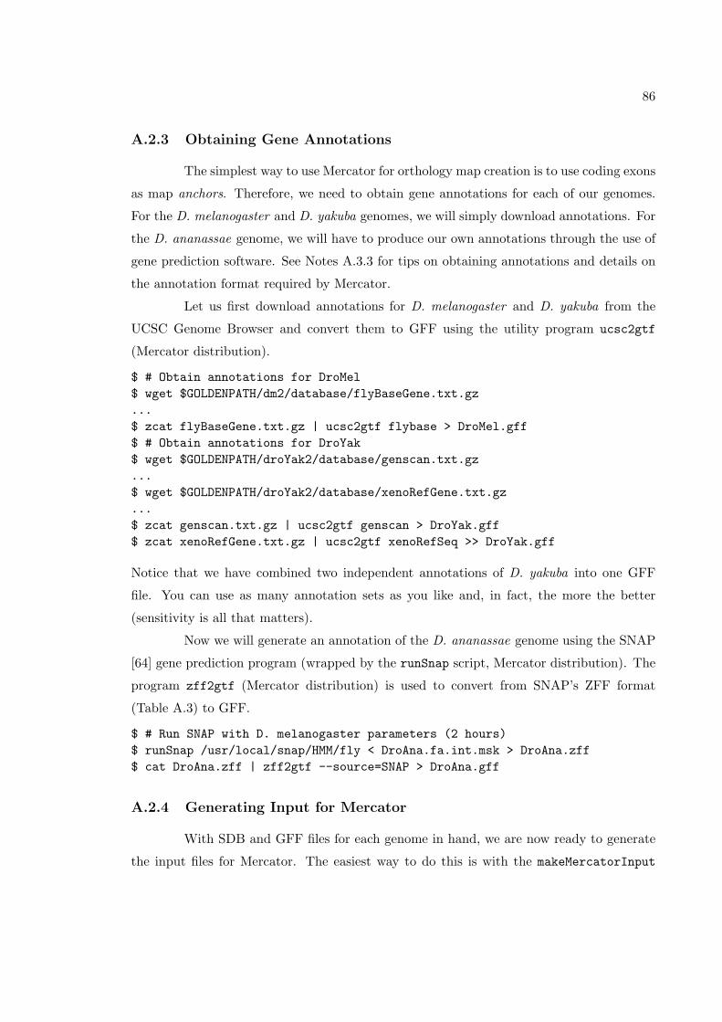
86

A.2.3 Obtaining Gene Annotations

The simplest way to use Mercator for orthology map creation is to use coding exons

as map anchors. Therefore, we need to obtain gene annotations for each of our genomes.

For the D. melanogaster and D. yakuba genomes, we will simply download annotations. For

the D. ananassae genome, we will have to produce our own annotations through the use of

gene prediction software. See Notes A.3.3 for tips on obtaining annotations and details on

the annotation format required by Mercator.

Let us first download annotations for D. melanogaster and D. yakuba from the

UCSC Genome Browser and convert them to GFF using the utility program ucsc2gtf

(Mercator distribution).

$ # Obtain annotations for DroMel$ wget $GOLDENPATH/dm2/database/flyBaseGene.txt.gz...$ zcat flyBaseGene.txt.gz | ucsc2gtf flybase > DroMel.gff$ # Obtain annotations for DroYak$ wget $GOLDENPATH/droYak2/database/genscan.txt.gz...$ wget $GOLDENPATH/droYak2/database/xenoRefGene.txt.gz...$ zcat genscan.txt.gz | ucsc2gtf genscan > DroYak.gff$ zcat xenoRefGene.txt.gz | ucsc2gtf xenoRefSeq >> DroYak.gff

Notice that we have combined two independent annotations of D. yakuba into one GFF

file. You can use as many annotation sets as you like and, in fact, the more the better

(sensitivity is all that matters).

Now we will generate an annotation of the D. ananassae genome using the SNAP

[64] gene prediction program (wrapped by the runSnap script, Mercator distribution). The

program zff2gtf (Mercator distribution) is used to convert from SNAP’s ZFF format

(Table A.3) to GFF.

$ # Run SNAP with D. melanogaster parameters (2 hours)$ runSnap /usr/local/snap/HMM/fly < DroAna.fa.int.msk > DroAna.zff$ cat DroAna.zff | zff2gtf --source=SNAP > DroAna.gff

A.2.4 Generating Input for Mercator

With SDB and GFF files for each genome in hand, we are now ready to generate

the input files for Mercator. The easiest way to do this is with the makeMercatorInput

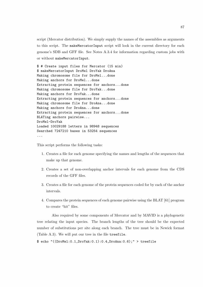
87

script (Mercator distribution). We simply supply the names of the assemblies as arguments

to this script. The makeMercatorInput script will look in the current directory for each

genome’s SDB and GFF file. See Notes A.3.4 for information regarding custom jobs with

or without makeMercatorInput.

$ # Create input files for Mercator (15 min)$ makeMercatorInput DroMel DroYak DroAnaMaking chromosome file for DroMel...doneMaking anchors for DroMel...doneExtracting protein sequences for anchors...doneMaking chromosome file for DroYak...doneMaking anchors for DroYak...doneExtracting protein sequences for anchors...doneMaking chromosome file for DroAna...doneMaking anchors for DroAna...doneExtracting protein sequences for anchors...doneBLATing anchors pairwise...DroMel-DroYakLoaded 10029188 letters in 98948 sequencesSearched 7247210 bases in 53254 sequences...

This script performs the following tasks:

1. Creates a file for each genome specifying the names and lengths of the sequences that

make up that genome.

2. Creates a set of non-overlapping anchor intervals for each genome from the CDS

records of the GFF files.

3. Creates a file for each genome of the protein sequences coded for by each of the anchor

intervals.

4. Compares the protein sequences of each genome pairwise using the BLAT [61] program

to create “hit” files.

Also required by some components of Mercator and by MAVID is a phylogenetic

tree relating the input species. The branch lengths of the tree should be the expected

number of substitutions per site along each branch. The tree must be in Newick format

(Table A.3). We will put our tree in the file treefile.

$ echo "((DroMel:0.1,DroYak:0.1):0.4,DroAna:0.6);" > treefile

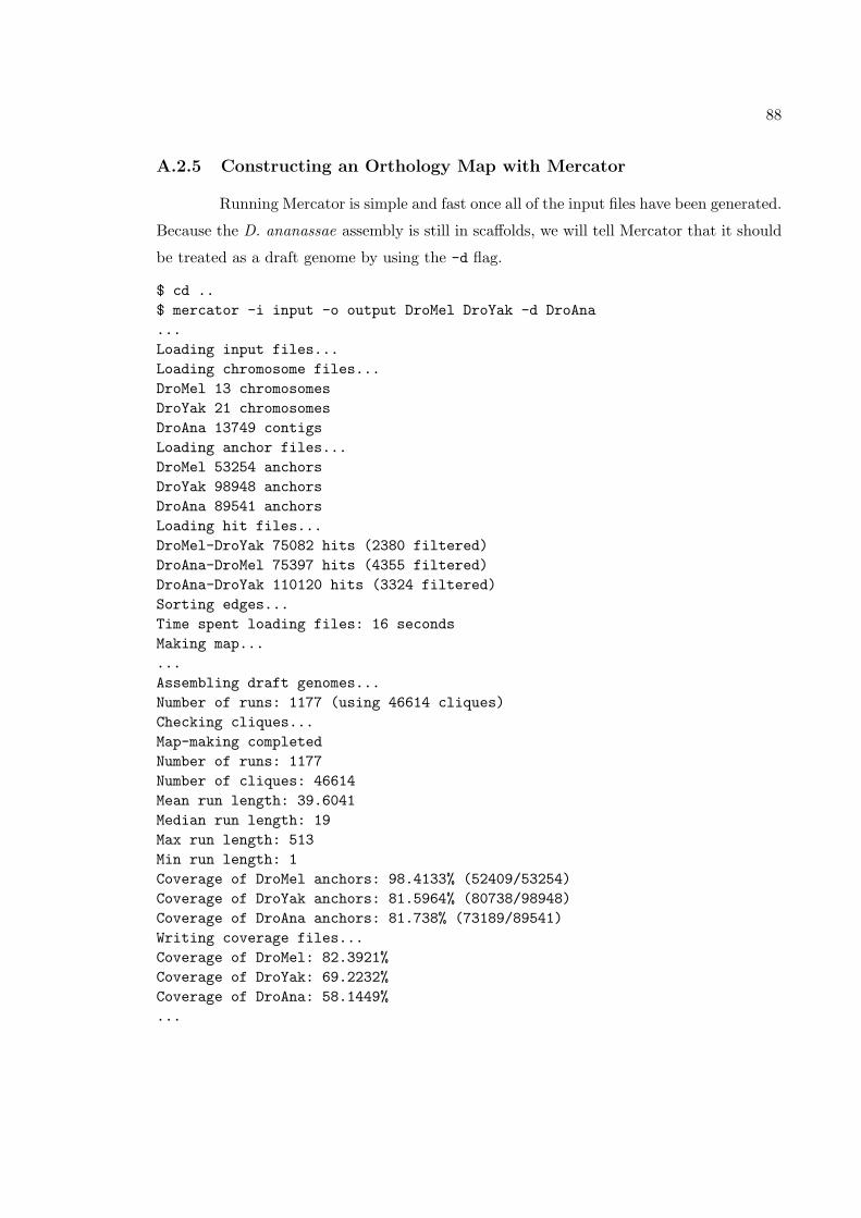
88

A.2.5 Constructing an Orthology Map with Mercator

Running Mercator is simple and fast once all of the input files have been generated.

Because the D. ananassae assembly is still in scaffolds, we will tell Mercator that it should

be treated as a draft genome by using the -d flag.

$ cd ..$ mercator -i input -o output DroMel DroYak -d DroAna...Loading input files...Loading chromosome files...DroMel 13 chromosomesDroYak 21 chromosomesDroAna 13749 contigsLoading anchor files...DroMel 53254 anchorsDroYak 98948 anchorsDroAna 89541 anchorsLoading hit files...DroMel-DroYak 75082 hits (2380 filtered)DroAna-DroMel 75397 hits (4355 filtered)DroAna-DroYak 110120 hits (3324 filtered)Sorting edges...Time spent loading files: 16 secondsMaking map......Assembling draft genomes...Number of runs: 1177 (using 46614 cliques)Checking cliques...Map-making completedNumber of runs: 1177Number of cliques: 46614Mean run length: 39.6041Median run length: 19Max run length: 513Min run length: 1Coverage of DroMel anchors: 98.4133% (52409/53254)Coverage of DroYak anchors: 81.5964% (80738/98948)Coverage of DroAna anchors: 81.738% (73189/89541)Writing coverage files...Coverage of DroMel: 82.3921%Coverage of DroYak: 69.2232%Coverage of DroAna: 58.1449%...

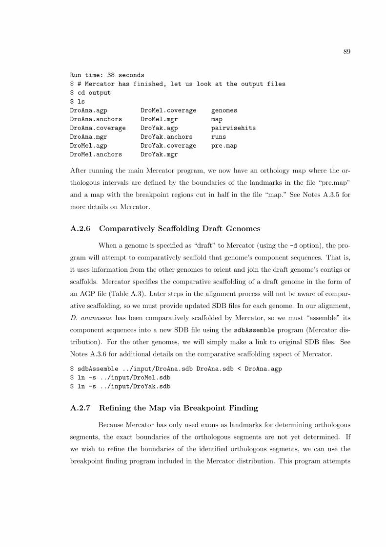
89

Run time: 38 seconds$ # Mercator has finished, let us look at the output files$ cd output$ lsDroAna.agp DroMel.coverage genomesDroAna.anchors DroMel.mgr mapDroAna.coverage DroYak.agp pairwisehitsDroAna.mgr DroYak.anchors runsDroMel.agp DroYak.coverage pre.mapDroMel.anchors DroYak.mgr

After running the main Mercator program, we now have an orthology map where the or-

thologous intervals are defined by the boundaries of the landmarks in the file “pre.map”

and a map with the breakpoint regions cut in half in the file “map.” See Notes A.3.5 for

more details on Mercator.

A.2.6 Comparatively Scaffolding Draft Genomes

When a genome is specified as “draft” to Mercator (using the -d option), the pro-

gram will attempt to comparatively scaffold that genome’s component sequences. That is,

it uses information from the other genomes to orient and join the draft genome’s contigs or

scaffolds. Mercator specifies the comparative scaffolding of a draft genome in the form of

an AGP file (Table A.3). Later steps in the alignment process will not be aware of compar-

ative scaffolding, so we must provide updated SDB files for each genome. In our alignment,

D. ananassae has been comparatively scaffolded by Mercator, so we must “assemble” its

component sequences into a new SDB file using the sdbAssemble program (Mercator dis-

tribution). For the other genomes, we will simply make a link to original SDB files. See

Notes A.3.6 for additional details on the comparative scaffolding aspect of Mercator.

$ sdbAssemble ../input/DroAna.sdb DroAna.sdb < DroAna.agp$ ln -s ../input/DroMel.sdb$ ln -s ../input/DroYak.sdb

A.2.7 Refining the Map via Breakpoint Finding

Because Mercator has only used exons as landmarks for determining orthologous

segments, the exact boundaries of the orthologous segments are not yet determined. If

we wish to refine the boundaries of the identified orthologous segments, we can use the

breakpoint finding program included in the Mercator distribution. This program attempts

90

to find the best position within each “breakpoint region” (intervals in between segments

identified in the “pre.map”) at which to break and add the left and right intervals to the

flanking segments. This procedure may be skipped if the exact boundaries of the segments

are not required. Locating breakpoints involves a number of steps. Note that SDB files

for each genome must be present in the current directory (output), as set up in the last

section. See Notes A.3.7 for additional information on the breakpoint finding process.

$ # The breakpoint finding algorithm requires the tree$ ln -s ../input/treefile$ # Convert the orthology map into a more general homology map$ omap2hmap genomes < pre.map > pre.h.map...$ # Create the graph relating the breakpoint regions$ makeBreakpointGraph pre.h.map treefile$ # Make pairwise alignments for breakpoint regions (2 hours)$ mkdir bp_alignments$ makeBreakpointAlignmentInput --out-dir=bp_alignments$ mavidAlignDirs --init-dir=bp_alignments$ # Find a good configuration of breakpoints (8 min)$ findBreakpoints pre.h.map treefile edges bp_alignments > breakpoints$ # Refine the map by splitting the breakpoint regions$ breakMap breakpoints < pre.h.map > better.h.map$ # Convert back to the orthology map format$ hmap2omap genomes < better.h.map > better.map

A.2.8 Generating Input for MAVID

Now that we have an orthology map, we are ready to run a global multiple align-

ment program on each orthologous segment set identified by the map. To help in the

alignment process, we will give the alignment program a set of “constraints”: short inter-

vals within the orthologous segments that we know should be aligned. These constraints

are derived from the sequence similarities identified between the anchors given to Mercator.

To make the constraints file, we run the following command:

$ # Convert pairwise hits to alignment constraints (2 min)$ phits2constraints -i ../input < pairwisehits > constraints

The input files for MAVID are then generated by makeAlignmentInput.

$ # Create directories and files for alignment (3 min)$ mkdir alignments$ makeAlignmentInput --map=better.map . alignments

91

See Notes A.3.8 for information on the input files that are required for MAVID and that

are generated by makeAlignmentInput.

A.2.9 Aligning Orthologous Segments with MAVID

With the input for MAVID generated, all that is left is to run MAVID on the

sequences for each orthologous segment set. Each segment set is stored in a separate sub-

directory. This is a good step at which to parallelize, but if that is not an option, the

mavidAlignDirs script (Mercator distribution) can be used. See Notes A.3.9 for details on

the nucleotide-level alignment step.

$ # Align all sequence files in directory structure (13 hours)$ mavidAlignDirs --init-dir=alignments

We now have a multiple whole-genome alignment of Drosophila melanogaster, Drosophila

yakuba, and Drosophila ananassae.

A.2.10 Extracting Subalignments

We may now extract parts of the whole-genome alignment that are of particu-

lar interest using the sliceAlignment program (Mercator distribution). For example, we

may wish to get the alignment of the second coding exon of the gene dachshund. The

sliceAlignment program outputs alignments in multi-FASTA format, so we will use the

fa2clustal utility (Mercator distribution) to put the exon alignment into a more readable

form. See Notes A.3.10 for more details on sliceAlignment.

$ sliceAlignment alignments DroMel chr2L 16477453 16477480 - > exon.mfa$ fa2clustal < exon.mfaCLUSTAL

DroMel ATGCCTATCGATCAAGCCACCAGAAAGDroYak ATGCCTATCGATCAAGCCACCAGAAAGDroAna ATGCCTATCGATCAAGCCACCAGAGAG

************************ **

92

A.3 Notes

A.3.1 Obtaining Genome Sequences

To download genomes from the UCSC Genome Browser, it is easiest to go through

the “Downloads” section of the Web site. For the assembly of interest, click on the “Full

data set” link to access complete genome sequences as compressed FASTA files (A.3). A

selection of Web sites that provide whole genome sequences is given in Table A.2.

A.3.2 Preparing the Genome Sequences

Masking Repeats

An “unmasked” FASTA formatted file has all characters in uppercase. A masked

sequence can either be “hardmasked” or “softmasked.” In hardmasked files, characters

that are part of repetitive sequence are changed to N’s, while in softmasked files they are

changed to lowercase. Unmasked and softmasked sequence may also have N’s, which are

commonly used to indicate assembly gaps. Ideally, we would like our genome sequences to

be softmasked, so that we have repeat annotations as well as full sequence information.

Masking repeats is a bit of an art, and I will not go into all of the details here.

Very briefly, one needs to mask both interspersed and simple (or low complexity) repeats.

Masking of these two types of repeats should be done separately because gene finding is

best done on sequence hardmasked for interspersed repeats (simple repeats can occur within

genes).

Creating Sequence Database Files

There are four command-line utilities made available in the Mercator distribution

for handling SDB files. The Mercator library code may also be used for writing C++

programs that access SDB files directly. The command-line utility fa2sdb is used to create

or append to a SDB file from sequence records in FASTA format. DNA sequences may be

compressed (2 nucleotides per byte) inside of a SDB file if the -c option is specified. The

sdbExport utility is used for the extraction of specific genomic intervals from a SDB file. It

can extract one or more intervals at a time and outputs sequences in FASTA format. The

sdbList utility is used to list the names and lengths (with the -l option) of the records

93

inside of a SDB file. Lastly, the fa2sdb utility is used to convert a SDB file into FASTA

format.

A.3.3 Obtaining Gene Annotations

Gene annotations for many genomes can be obtained at the same database sites

that provide whole genome sequences. For the UCSC Genome Browser site, annotations

can be obtained either through the “Table Browser,” or directly from the “Downloads”

section. If annotations are not available online, you can produce them using gene prediction

software. The easiest prediction programs to use in this case are single-genome ab initio

gene finders (e.g., geneid [47], GENSCAN [17], and SNAP [64]). Regardless of how the

annotations are obtained, they need to be converted to the GFF format (Table A.3). Three

scripts (genscan2gtf, ucsc2gtf, and zff2gtf) in the Mercator distribution are available

for converting to GFF from some common formats. Mercator requires that GFF annotations

have CDS records (lines with “CDS” in the feature field) for the coding intervals of each

exon. It is critical that the “frame” field be specified for each CDS record in the GFF files.

This field allows Mercator to translate each coding exon correctly.

A.3.4 Generating Input for Mercator

For custom jobs (e.g., to parallelize some tasks), you may wish to generate the

input for Mercator without using the makeMercatorInput script. In such cases, consult the

README file in the Mercator distribution for exact specifications of the various input files

that are required. Some routines of makeMercatorInput are customizable via command-line

options. Use the use --help option to get full usage information.

A.3.5 Constructing an Orthology Map with Mercator

Mercator has a number of user-settable parameters that may be speci-

fied as command-line options. The options that affect Mercator’s performance are

--min-run-length, --prune-pct, --join-distance, --max-eval, --repeat-num, and

--repeat-pct. Consult the Mercator README file for descriptions of these options.

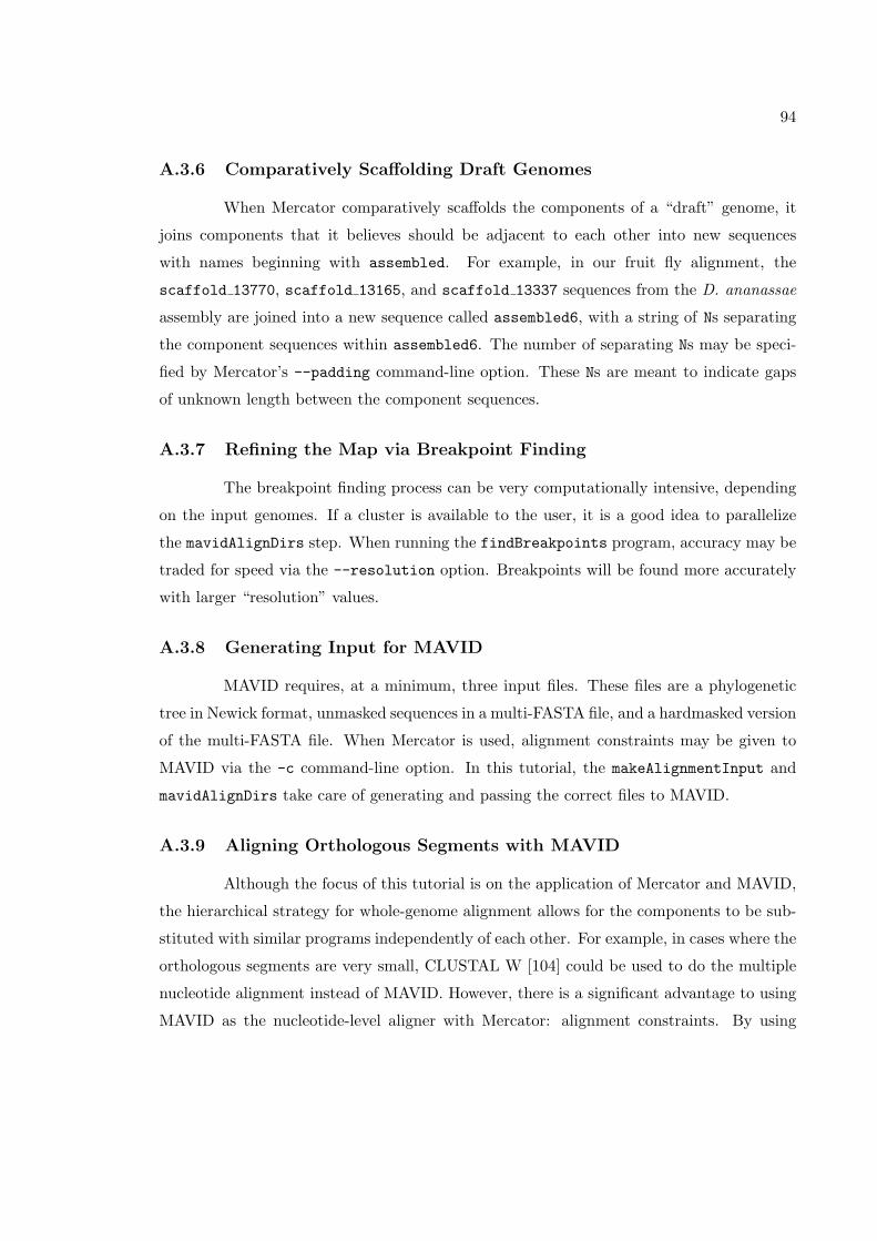
94

A.3.6 Comparatively Scaffolding Draft Genomes

When Mercator comparatively scaffolds the components of a “draft” genome, it

joins components that it believes should be adjacent to each other into new sequences

with names beginning with assembled. For example, in our fruit fly alignment, the

scaffold 13770, scaffold 13165, and scaffold 13337 sequences from the D. ananassae

assembly are joined into a new sequence called assembled6, with a string of Ns separating

the component sequences within assembled6. The number of separating Ns may be speci-

fied by Mercator’s --padding command-line option. These Ns are meant to indicate gaps

of unknown length between the component sequences.

A.3.7 Refining the Map via Breakpoint Finding

The breakpoint finding process can be very computationally intensive, depending

on the input genomes. If a cluster is available to the user, it is a good idea to parallelize

the mavidAlignDirs step. When running the findBreakpoints program, accuracy may be

traded for speed via the --resolution option. Breakpoints will be found more accurately

with larger “resolution” values.

A.3.8 Generating Input for MAVID

MAVID requires, at a minimum, three input files. These files are a phylogenetic

tree in Newick format, unmasked sequences in a multi-FASTA file, and a hardmasked version

of the multi-FASTA file. When Mercator is used, alignment constraints may be given to

MAVID via the -c command-line option. In this tutorial, the makeAlignmentInput and

mavidAlignDirs take care of generating and passing the correct files to MAVID.

A.3.9 Aligning Orthologous Segments with MAVID

Although the focus of this tutorial is on the application of Mercator and MAVID,

the hierarchical strategy for whole-genome alignment allows for the components to be sub-

stituted with similar programs independently of each other. For example, in cases where the

orthologous segments are very small, CLUSTAL W [104] could be used to do the multiple

nucleotide alignment instead of MAVID. However, there is a significant advantage to using

MAVID as the nucleotide-level aligner with Mercator: alignment constraints. By using

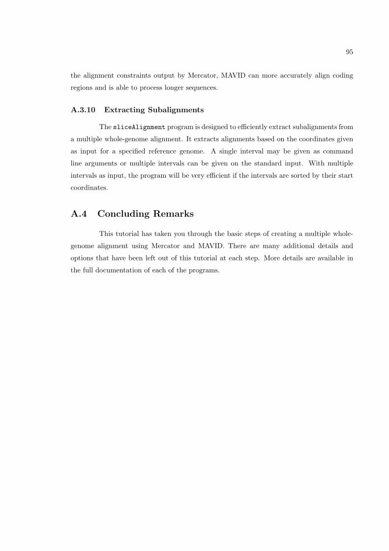
95

the alignment constraints output by Mercator, MAVID can more accurately align coding

regions and is able to process longer sequences.

A.3.10 Extracting Subalignments

The sliceAlignment program is designed to efficiently extract subalignments from

a multiple whole-genome alignment. It extracts alignments based on the coordinates given

as input for a specified reference genome. A single interval may be given as command

line arguments or multiple intervals can be given on the standard input. With multiple

intervals as input, the program will be very efficient if the intervals are sorted by their start

coordinates.

A.4 Concluding Remarks

This tutorial has taken you through the basic steps of creating a multiple whole-

genome alignment using Mercator and MAVID. There are many additional details and

options that have been left out of this tutorial at each step. More details are available in

the full documentation of each of the programs.

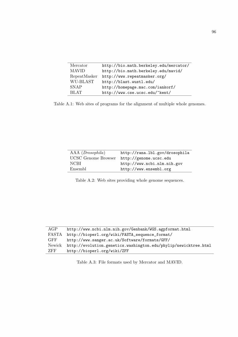
96

Mercator http://bio.math.berkeley.edu/mercator/MAVID http://bio.math.berkeley.edu/mavid/RepeatMasker http://www.repeatmasker.org/WU-BLAST http://blast.wustl.edu/SNAP http://homepage.mac.com/iankorf/BLAT http://www.cse.ucsc.edu/~kent/

Table A.1: Web sites of programs for the alignment of multiple whole genomes.

AAA (Drosophila) http://rana.lbl.gov/drosophilaUCSC Genome Browser http://genome.ucsc.eduNCBI http://www.ncbi.nlm.nih.govEnsembl http://www.ensembl.org

Table A.2: Web sites providing whole genome sequences.

AGP http://www.ncbi.nlm.nih.gov/Genbank/WGS.agpformat.htmlFASTA http://bioperl.org/wiki/FASTA_sequence_format/GFF http://www.sanger.ac.uk/Software/formats/GFF/Newick http://evolution.genetics.washington.edu/phylip/newicktree.htmlZFF http://bioperl.org/wiki/ZFF

Table A.3: File formats used by Mercator and MAVID.