Who Benefits from Accountability-Driven School Closure ... · Jun Cai, ECON . Ziqiao Chen, PAIA ....
70
Who Benefits from Accountability-Driven School Closure? Evidence from New York City Robert Bifulco, Jr. and David Schwegman Paper No. 212 December 2018
Transcript of Who Benefits from Accountability-Driven School Closure ... · Jun Cai, ECON . Ziqiao Chen, PAIA ....

Who Benefits from Accountability-Driven School Closure? Evidence from New York City
Robert Bifulco, Jr. and David Schwegman
Paper No. 212 December 2018

CENTER FOR POLICY RESEARCH – Fall 2018
Leonard M. Lopoo, Director Professor of Public Administration and International Affairs (PAIA)
Associate Directors Margaret Austin
Associate Director, Budget and Administration
John Yinger Trustee Professor of ECON and PAIA
Associate Director, Metropolitan Studies
SENIOR RESEARCH ASSOCIATES
Badi Baltagi, ECON Robert Bifulco, PAIA Leonard Burman, PAIA Carmen Carrión-Flores, ECON Alfonso Flores-Lagunes, ECON Sarah Hamersma, PAIA Madonna Harrington Meyer, SOC Colleen Heflin, PAIA William Horrace, ECON Yilin Hou, PAIA
Hugo Jales, ECON Jeffrey Kubik, ECON Yoonseok Lee, ECON Amy Lutz, SOC Yingyi Ma, SOC Katherine Michelmore, PAIA Jerry Miner, ECON Shannon Monnat, SOC Jan Ondrich, ECON David Popp, PAIA
Stuart Rosenthal, ECON Michah Rothbart, PAIA Alexander Rothenberg, ECON Rebecca Schewe, SOC Amy Ellen Schwartz, PAIA/ECON Saba Siddiki, PAIA Perry Singleton, ECON Yulong Wang, ECON Michael Wasylenko, ECON Peter Wilcoxen, PAIA
GRADUATE ASSOCIATES
Rhea Acuna, PAIA Jun Cai, ECON Ziqiao Chen, PAIA Yoon Jung Choi, PAIA Stephanie Coffey, ECON Jordana Gilman, Lerner Emily Gutierrez, PAIA Jeehee Han, PAIA Daniel Hiller, PAIA Yusun Kim, PAIA
Hyoung Kwon, PAIA Judith Liu, ECON Rob Loomis, PAIA Maeve Maloney, ECON Qasim Mehdi, PAIA Angie Mejia, Lerner Katie Mott, Lerner Christina Parsons, PAIA Jonathan Presler, ECON Krushna Ranaware, SOC
Christopher Rick, PAIA David Schwegman, PAIA Iuliia Shybalkina, PAIA Stephanie Spera, Lerner Mackenzie Theobald, PAIA Saied Toossi, PAIA Huong Tran, ECON Joaquin Urrego, ECON Sean Withington, Lerner Yi Yang, ECON
STAFF
Joanna Bailey, Research Associate Joseph Boskovski, Maxwell X Lab Katrina Fiacchi, Administrative Specialist Emily Minnoe, Administrative Assistant
Kathleen Nasto, Administrative Assistant Candi Patterson, Computer Consultant Laura Walsh, Administrative Assistant
DRAFT: PLEASE DO NOT CITE OR CIRCULATE WITHOUT AUTHORS’ PERMISSION
Abstract
We estimate the effects of accountability-driven school closure in New York City on students who
attended middle schools that were closed at the time of closure and students who would have likely
attended a closed middle school had it remained open. We find that students who would have entered
the closed school, had it not closed, attended schools that perform better on standardized exams and
have higher value-added measures than did the closed schools. While we find that closure did not have
any measurable effect on the average student in this group, we do find that high-performing students
in this group attended higher-performing schools and experienced economically-meaningful and
statistically-significant improvements in their sixth, seventh, and eighth-grade math test scores. We
find that these benefits persisted for several cohorts after closure. We also find that closure adversely
affected students, low-performing students in particular, who were attending schools that closed. For
policymakers, our results highlight a key tradeoff of closing a low-performing school: future cohorts of
relatively high-performing students may benefit from closure while low-performing students in schools
designated for closure are adversely affected.
JEL Codes: I20, I21, I28
Keywords: School Closure, School Accountability, Urban School Reform
Authors: Robert Bifulco, Jr. and David Schwegman, Center for Policy Research, Department of Public Administration and International Affairs, Maxwell School of Citizenship and Public Affairs, Syracuse University

DRAFT: PLEASE DO NOT CITE OR CIRCULATE WITHOUT AUTHORS’ PERMISSION
1
I. Introduction
Closing a school is an increasingly common response to low student performance. No Child Left Behind
(NCLB) and the Race to the Top initiative included closure as a possible accountability option that districts
could impose on schools that fail to make adequate yearly progress (Kemple 2015, Capps et al. 2005). In
recent years, cities throughout the United States, including Chicago, Denver, Pittsburg, Hartford, among
others, have closed schools due to a combination of declining enrollment and accountability reasons (Engberg
et al. 2011, Steiner 2009). Proponents argue that policies that close the lowest-performing schools make it
likely that students who would have attended these schools will attend higher-quality schools and thus have a
greater chance at academic success. Opponents argue that school closures can be academically and socially
disruptive, destabilize peer networks, increase time spent traveling to school, and expose students to violence
if they are forced to travel into different neighborhoods (de la Torre and Gwynne 2009).
The empirical evidence on school closure is mixed. Some scholars find that school closure can be
disruptive and negatively affect a student’s academic career, while others find small positive or, more
commonly, null effects of closure on student performance (CREDO 2017, Kemple 2015, Brummet 2014, de
la Torre et al. 2015, Engberg et al. 2011, de la Torre and Gwynne 2009). While insightful, this literature suffers
from two limitations. First, most of these studies intermingle school closures caused by low or declining
enrollment and school closures solely due to accountability reasons (exceptions, see Kemple 2015, Carlson
and Lavertu 2016). Districts with declining enrollments often close a large proportion of schools at once, which
can be disruptive for students who attend the closed schools and students in schools that remain open and
receive a large influx of students. In these situations, it is challenging to disentangle the potentially beneficial
effects of closing underperforming schools from the disruptive effects of reorganizing the district into a smaller
number of schools. Second, most studies examine the effects of closure on students attending a school when it

DRAFT: PLEASE DO NOT CITE OR CIRCULATE WITHOUT AUTHORS’ PERMISSION
2
was closed. While this is a critical group to study to inform school closure implementation, it is also a group that
may be particularly likely to experience negative disruption effects because of a school closure. Another group
that may benefit from the closure of a low-performing school without suffering excessive disruption effects are
younger cohorts of students who would have attended the closed school later had it not closed. Without
considering the effect of closure on both groups of students, studies of school closure fail to capture the full
effects of closure on academic outcomes.1
Our study addresses these limitations by examining accountability-driven middle school closure in
New York City on both groups of students. In New York City, school closure is implemented using a phaseout
process. Under this process, schools slated for closure stop enrolling new students and eliminate the entry
grade in the school. Students who are attending the school at that time are given the option of remaining at the
school until the school’s terminal grade or transferring to another school in the district. We estimate the effects
of closure on students attending schools at the time of closure (whom we call students in the phaseout cohorts)
and students who would have entered the school after closure had it not closed (whom we call students in the
closure cohorts).
To estimate the effects of school closure on students who would have likely attended a closed school
had it remained open, we use pre-closure information on individual students and school feeder patterns to
identify cohorts of students who would have likely attended a closed school. Next, we estimate the effects of
closure using a difference-in-differences strategy that compares cohorts of students affected by closure to
earlier cohorts in the same school controlling for changes across contemporaneous cohorts in schools that have
not yet closed.
1 School closure can also affect students in schools that receive displaced students due to closure (Brummet 2014; Engberg et al. 2012). While we do not believe our context is the best one to study these effects, we do examine this question in Section VII below.

DRAFT: PLEASE DO NOT CITE OR CIRCULATE WITHOUT AUTHORS’ PERMISSION
3
We find that closure caused students who would have entered the closed school (i.e. students in the
closure cohorts) to travel farther to attend schools that have fewer students from their school in the previous
grade and that have higher average levels of student performance than they would have had the school not
closed. On average, closure is not significantly associated with improved academic performance among
students in the closure cohorts. However, we do find that the effects of closure on distance traveled to school,
percent of students from the student’s previous school, and average school achievement are larger for higher-
achieving students in the closure cohort than lower-achieving students in that group, and that closure has
positive effects on the achievement of relatively high-performing students in the closure cohorts. We also find
these positive effects for high-performing students in each of the first three cohorts who would have entered
the school in years following closure. For each cohort, we find these positive effects first emerge in sixth grade
and persist until at least eighth grade.
We also find that students already in the closed school when it is designated for closure (i.e. students
in the phaseout cohorts) transfer out of their sixth-grade middle school at higher rates than students in schools
that have not yet initiated closure and that, on average, the schools these students attend are similar to the
closed schools on a range of observable characteristics. By eighth grade, students in the phaseout cohorts have
measurably lower performance and higher absentee rates, on average, than they would have in the absence of
school closure. We find these negative effects are largely borne by lower-performing students in the phaseout
cohorts (those in the lowest three quintiles of pre-closure performance). We also find that the displacement of
phaseout and closure students to other schools (i.e. spillover into receiving schools) had no effect on students
in the schools that phaseout and closure students attended following closure.
These results indicate that, in an urban environment with a high density of educational options that are
higher performing than the closed school, school closures can benefit some of the students who would have

DRAFT: PLEASE DO NOT CITE OR CIRCULATE WITHOUT AUTHORS’ PERMISSION
4
attended the closed school. We present evidence that, in New York City, relatively-higher-achieving students
may have had easier access to relatively higher-quality school options. These higher-achieving students also
tended to be the students who benefited from closure decisions. However, when a phaseout process that
provides students currently attending a school designated for closure the option of either remaining in that
school or transferring elsewhere, gains for students in future cohorts might come at the expense of students,
particularly low-performing students, who are attending schools at the time of closure.
These results have two key policy implications. First, our results suggest that providing students who
would otherwise attend a closed school alternative schooling options that are higher quality than the closed
school may be key to realizing achievement gains. A failure to provide more high-quality options for low-
performing students who would have attended closed school might be a reason New York City’s school
closures did not achieve broader performance gains. Second, by identifying the specific groups that benefit
from and who are harmed by an accountability-driven school closure policy, our analyses highlight an important
potential trade-off posed by school closure decisions. Of particular concern in New York City is that while high-
achieving students in future cohorts tended to benefit from closure, lower-performing students who had
already started in closed schools tended to be made worse off.
The next section provides a brief description of school closure in New York City. Section III provides a
simple conceptual model to understand how the disruptive effects of school closure and the quality of the
school students attend following closure will likely mediate the effect of closure on student performance, as
well as a review of previous empirical evidence on the effects of school closure. Sections IV and V describe our
data and analytical strategy, and we present our results in section VI. In section VII, we discuss the potential
negative spillovers of closure on students in the schools receiving students who otherwise would have attended
a closed school. We provide tests of our identifying assumptions and provide a supplementary analysis to

DRAFT: PLEASE DO NOT CITE OR CIRCULATE WITHOUT AUTHORS’ PERMISSION
5
examine the degree to which school environment mediates the main effect of closure in Section VIII. Section IX
concludes with a summary of our key findings and a discussion of their policy implications.
II. School Closure in New York City
School closure implies the end of a school as an administrative entity. While related accountability
actions, such as restructuring and school conversion, imply that there is some continuity in the student body
and, in some cases, the staff (Kirshner, Gaertner, and Pozzoboni 2011), “school closure” means that all
administrative and instructional staff transfer to other schools and students no longer enroll in the school.2 In
the United States, a school district chooses to close a school for two primary reasons—declining enrollment and
low performance (Steiner 2009). Many districts faced with declining enrollments use student and school
performance indicators to help identify which schools to close (see Engberg et al. 2011, de la Torre et al. 2015).
New York City, following the passage of No Child Left Behind, implemented a high-stakes
accountability system based primarily on student academic outcomes. As part of this accountability system,
the NYC Department of Education (NYC DOE) pursued the closure of schools that continually failed to meet
performance standards. All schools identified for closure were first designated as persistently lower-achieving
schools by the New York State Department of Education. A school is designated as persistently low achieving
if a school’s English Language Art and Math state test scores are in the bottom five percent of all schools in New
York State, and the school fails to improve its performance on this metric over the next three years. Once a
school is designated as persistently low achieving, NYC DOE would either select a school for “turnaround” or
“phaseout.” According to Educational Impact Statements and conversations with officials at the NYC
Department of Education, schools with chronically low attendance—bottom 10 percent of the district and
2 In many cases, a new school or schools with different staff and feeder patterns, and perhaps a different grade configuration, are located in the vacated building, but these new schools are different administrative and educational entities than the schools they replace.

DRAFT: PLEASE DO NOT CITE OR CIRCULATE WITHOUT AUTHORS’ PERMISSION
6
schools with poor grades from their Quality Review evaluations were selected for phaseout. Quality Reviews
assess the ability of a school to reform quickly in response to the needs of their students.3
As described in Kemple (2015), the process by which affected students and communities are notified
of the decision to close a school evolved between 2003-04 and 2012-13. New York City’s initial closure
process was opaque with little public input (Kemple 2015, Steiner 2009). In 2009, New York City codified its
school closure policy in the NYC DOE Regulation of the Chancellor (A-190). Under A-190, six months before
any closure decision, the Chancellor of NYC schools must publically provide an “educational impact statement”
that assesses the impact of the closure on the affected students and proposes a plan to reassign these students
to other schools. Students and parents in these schools are notified, and the Chancellor’s Office holds a public
meeting and solicits public input. Following a public hearing and a publicly-posted response to submitted
comments, the Panel for Education Policy (PEP) can approve or reject the Chancellor’s proposal.
NYC publicly posts the PEP’s decisions and school closure documentation dating back to the 2009-10
academic year. Since 2009-10, the Chancellor has initiated the closure process between August and October
in most academic years. The PEP voted on 79 of the 87 proposals sometime between the following January and
April. Of the 79 phaseout proposals considered by the PEP between the 2009-10 and 2011-12 academic
year, 65 were passed, 2 were scheduled to be considered at some later date, and 12 were withdrawn from
consideration. The PEP has never formally rejected a proposal to close a school. If the PEP approves the closure
3 Persistently low achieving schools with moderate to high Quality Review grades were selected for “turnaround.” These schools were required to implement a teacher evaluation system and alter instructional and student support systems. Additional funds were often provided to turnaround schools to support these programs. The De Blasio Administration ended the Bloomberg Administration’s School Closure when it came to office in 2013. They designated all persistently low achieving schools to be turnaround schools, which reflects the controversy around the school closure policy. However, in December 2017, it was announced that the De Blasio Administration would begin to close some of the schools that it designated for turnaround.

DRAFT: PLEASE DO NOT CITE OR CIRCULATE WITHOUT AUTHORS’ PERMISSION
7
proposal, phaseout begins in the academic year following approval. When a school begins phaseout, new
students are no longer admitted to the school. The students already enrolled in the school when a school is
designated for closure can remain there until the school’s terminal grade or transfer to another school. Since the
2002-2003 academic year, 157 schools have closed in New York City, including 47 middle schools.4
In New York City, students transitioning from elementary to middle school have a substantial degree
of choice among public schools, which influences both which students would have attended closed schools and
where they enroll instead. Students entering sixth grade apply to middle schools during the Middle School
Admission process, which begins in November in the year prior to moving to middle school (in fifth-grade for
most students). Students are eligible to attend programs in their community school district, borough-wide
programs in their home borough, or citywide programs that are open to all NYC students. Students are
guaranteed a place in their zoned middle school and students who were zoned for a middle school that closes
are assigned to the zone of a different middle school. Whether a student is admitted to another school to which
they apply is determined at the school-level, either through a selective-admission process, through a lottery, or
some other admissions process.
Some schools do evaluate past academic performance and attendance records when considering which
students to admit. These admission priorities likely constrain the educational options for lower-achieving
students relative to higher-achieving students. In the online Appendix (see Table A1), we quantify the number
of options available in the 2007-08 year for the students in the 21 community school districts in which our
closures occurred.
4 Figure A1 in the online Appendix provides a map that places the 47 closures in our paper in their respective community school district.

DRAFT: PLEASE DO NOT CITE OR CIRCULATE WITHOUT AUTHORS’ PERMISSION
8
We find that students had, on average, 35 options available to them.5 If we exclude schooling options
that consider test scores, course grades, and/or selective admissions tests as admission priorities, which would
privilege higher-performing students, the number of options available to the typical student who would have
attended a closed school is 20 schools. Thus, if we assume that high-performing students have access to all
schools and low performing student have access only to those without academic admission criteria, then a
higher-performing student has 77 percent more options than low-performing students. Moreover, a majority
of the schools that use academic admission standards have value-added measures that are above the citywide
average, while far smaller proportions of other schooling options have above average value-added. If we
assume only high achievers can access schools with academic admission criteria, then, in the average
community school district, high-performing students have access to more than two times as many schools with
above average value-added as do low-performing students. Of course, in individual cases, the number of
options effectively available to a low-performing student might be greater or the options effectively available
to a high-performing student might be less than the numbers in Table A1 indicate. Nonetheless, these figures
provide clear indication that high-achieving students are likely to have more high-quality schooling options
available to them than low-achieving students.
Students in the phaseout cohorts can transfer following closure. Their options, however, are
constrained by the number of schools receiving transfer students and the number of seats available in those
schools. Thus, the ability to transfer to a school with higher levels of student achievement or other desirable
qualities is much more constrained for students in the phaseout cohort than students in the closure cohort, and
options for low-achieving students in the phaseout cohorts may be particularly limited.
5 These options include each student’s zone school, the un-zoned schools in their community school district, the borough-wide options available to students, and the city-wide options available to students.

DRAFT: PLEASE DO NOT CITE OR CIRCULATE WITHOUT AUTHORS’ PERMISSION
9
Given the ample choice available to students, none of the school closures we examine result in a large
influx of new students into any single school. Among the schools that ever received a sixth student that we
estimate would have otherwise attended a closed school, the median percent of sixth graders who otherwise
would have been in a closed school is only 4 percent, and for very few schools is this percentage ever greater
than 15 percent in any year (see top panel of Figure 1). Similarly, among schools that ever received a seventh
or eighth-grade student from a school during phaseout, the median percent of seventh and eighth graders from
a phaseout school is 2.6 percent of the student body, and in no school was this percentage ever more than 10
percent (see bottom panel of Figure 1). Given these low proportions, our primary empirical strategy assumes
that there are no spillovers onto students in the receiving schools. In section VII, we present estimates of the
effect of school closure on students in the receiving schools and find no evidence of spillover onto these
students.
III. Conceptual Framework and Literature Review
The relationship between school closure and student performance is theoretically ambiguous and, as
depicted in Figure 2, is likely to be mediated by the quality of the receiving school to which a student sorts and
the level of dislocation experienced by the student during the closure process. In the analysis below, we
estimate the effects of school closure on a number of factors that might influence school quality with some
emphasis on factors that might be related to improved student academic performance. Since accountability-
driven school closure focuses on the lowest-performing schools, we expect that, on average, students in the
closure cohorts will find their way into schools with characteristics more conducive to student academic
success. However, because the options of students in the phaseout cohorts are more constrained, particularly
among low-achieving students, and because the phaseout process might degrade the quality of schooling in the

DRAFT: PLEASE DO NOT CITE OR CIRCULATE WITHOUT AUTHORS’ PERMISSION
10
schools being closed, we might expect a decrease in school quality for many of the students in the phaseout
cohorts.
Dislocation or disruption refers to the effects of a student moving to a new environment. There is a
consensus among scholars that student mobility has adverse effects on student performance in the period
immediately following a move (Hanusek, Kain, and Rivkin 2004). When a school is closed, closure-induced
student displacement may adversely affect a student’s behavior and academic outcomes. Students may need
to travel farther distances and into new neighborhoods to attend school, cope with changes in school
environment and culture, and develop new peer networks.
Different types of students are likely to respond differently to phaseout and closure (de la Torre and
Gwynne 2009, Özek et al. 2012, Kirshner, Gaertner, and Pozzoboni 2011). For example, compared to lower-
achieving students, high-achieving students might be more likely to transfer out of a school designated for
closure during the phaseout period and/or might choose alternative schools with high-achieving students,
either because they have more access to such schools or because they and their parents place greater value on
high levels of achievement. Also, higher-achieving students might be more (or less) resilient to dislocation
effects and/or benefit more from attending a school with higher average levels of student achievement. We
thus expect the effects of school closure on both school quality and disruption will vary by student background
characteristics, and particularly by past the past achievement level of a student (Özek, Hansen, and Gonzalez
2012).
Evidence from previous empirical work on school closure is mixed. Some scholars have found positive
effects of school closure on student performance (Bross, Harris, and Liu 2016; Brummet 2014; Carlson and
Lavertu 2016; Kemple 2015), while others find negative or null effects (de la Torre and Gwynne 2009;

DRAFT: PLEASE DO NOT CITE OR CIRCULATE WITHOUT AUTHORS’ PERMISSION
11
Engberg et al. 2012; Kirshner, Gaertner, and Pozzoboni 2010; Ozek, Hansen, and Gonzalez 2012). In addition
to providing mixed results, the existing empirical literature suffers from two primary limitations.
First, most studies comingle closures due to declining enrollment with accountability-driven closures
(Sunderman and Payne 2009). For instance, Brummet (2014) examines 200 school closures throughout
Michigan, many of which were consolidation-driven and some of which were accountability-driven.6 Because
effects on school quality and dislocation are likely to differ across these two types of closures, it is difficult to
know how to generalize the results from these studies to a context in which a school district uses an
accountability-based policy to close public schools. In New York City, school closure was an accountability tool
targeted for chronically poor-performing schools. This policy was not part of a school consolidation effort.
Second, most studies focus on the effects of closure on students attending the school at the time of
closure and/or students in schools that receive a large influx of students from the closed schools (e.g., Brummet
2014, Engberg et al. 2012). The effects on these groups of students are important to understand, but school
closure policies are also intended to benefit future students, i.e. students who would have entered the school in
later years in the absence of closure. Disruption effects are likely to be less marked for these future students
than for students currently in the school, so effects on the two groups of students may differ. One exception is
Kemple (2015), which uses an approach similar to the one we use to identify students who were likely to have
attended a closed school and finds that the closure of New York City high schools had a positive effect on the
graduation rates of those students.
Several aspects of the New York City context allow us to contribute to the existing literature. First,
nearly all of the students in the sample we use to estimate effects on sixth-grade outcomes are making a
6 Carlson and Levertu (2016), which attempts to identify the effect of school closure based on a school value-added accountability cutoff, is an important exception.

DRAFT: PLEASE DO NOT CITE OR CIRCULATE WITHOUT AUTHORS’ PERMISSION
12
transition from elementary to middle school.7 As a result, both students in the treatment and comparison
groups are experiencing a change of schools between fifth and sixth grade, and thus both groups experience
some degree of natural disruption that would have occurred in the absence of treatment. The disruption that
accompanies the move from elementary to middle school might be greater for students affected by school
closure, for instance, they might have to attend a school further from their home or accompanied by fewer
students from their elementary school. Nonetheless, the added disruptive effect of closure for students in our
closure cohort is smaller than for students dislocated from their current school. Second, no school received a
large influx of students from the closed schools, which minimizes any disruptions experienced by students in
the receiving schools. Third, NYC targeted closure to its lowest-performing schools which increases the
likelihood that students who would have attended the closed schools are moved into higher-quality schools as
a result of the closure. These features allow us to estimate the effects of changes in school quality that result
from school closure in an environment where disruption is minimized. Thus, our results are particularly relevant
for understanding the long-run effects of school closure policies that make it likely students will attend a higher-
quality school.
We also contribute to the literature by refining the approach used by Kemple (2015) and estimating
the effects of school closure on students who are likely to have attended a school that closed, an understudied
group. Finally, we investigate the heterogeneity of school closure impacts across different types of students.
IV. Data and Sample
This study uses individual student data for the years 2001-02 through 2014-15 provided by the NYC
DOE. These data include information on student race/ethnicity, free-and-reduced-price lunch eligibility status,
7 Of our primary estimation sample, 96.4 percent were in schools that ended in fifth grade and thus would need to transfer. The remaining 3.6 percent were in K-8 or K-12 schools and thus could remain in their schools if they chose.
DRAFT: PLEASE DO NOT CITE OR CIRCULATE WITHOUT AUTHORS’ PERMISSION
13
disability status, home zip code, attendance record, and performance on state exams that can be linked over
time. The data also identify the school the student attends as of October 31 of each year, which allows us to
merge in school-level data also from the NYC DOE. These school-level data include the percent of students in
each race/ethnicity category, the percent who are free-and-reduced-price lunch eligible, geographical location
information, and the grade-specific absentee rate.
For our primary analysis, we focus on students who attended or are likely to have attended one of the
47 middle schools that closed between 2004-05 and 2012-13.8 For each of these 47 schools, we define a
year-specific cohort as the set of students who enter sixth grade in that school in that year. Using a method
described below, we also identify for each school a set of students who are likely to have entered the school in
the first year after the phaseout component of closure is initiated. Compared to previous studies of school
closures with shorter panels, such as Engberg et al. (2012) or Brummet (2014), we are able to exploit this long
panel of student-cohorts for each closed school in order to test the underlying assumption of our difference-in-
differences strategy.
Table 1 provides summary statistics on the students in the 2003-04 cohorts of the schools that
eventually closed sometime between 2004-05 and 2012-13. The statistics include means and standard
deviations of both individual variables and school-level characteristics for this sample of students. We also
provide similar statistics for all other sixth-grade students in the district who were attending a grades 6-8
school. Compared to students in the rest of the district, students in schools that eventually close are more likely
to be black and Hispanic and less likely to be white and Asian, more likely to be eligible for free-or-reduced-
8 For the analyses used to identify students who are likely to have attended one of the closed schools, we use a broader set of students.

DRAFT: PLEASE DO NOT CITE OR CIRCULATE WITHOUT AUTHORS’ PERMISSION
14
price lunch, have a higher absentee rate, and lower normalized scores on sixth-grade math and ELA exams.9
The school-level characteristics follow a similar pattern, with our closed schools being much lower-performing
and containing fewer white and Asian students than the average school enrolling sixth-graders in the district.
Given the marked differences between students who attended schools that close and those that attend
other New York City schools, it is difficult to draw conclusions about the effect of school closure from
comparisons of students who are likely to have attended closed schools and students in other New York City
middle schools. Instead, we limit comparison in this study to changes in outcomes across cohorts in schools that
closed earlier and changes in outcomes across cohorts in schools that closed later. Table 2 compares the sixth-
grade cohorts in schools that closed in each year to same-year sixth-grade cohorts in the schools that began
phaseout in later years. In the year before phaseout began, closed schools were similar on observed covariates
to schools that would begin phaseout later. We do not find any statistically significant differences in these
school-level covariates across schools closed in the current year and schools closed later. However, given that
only a single school closed in the 2012-2013 academic year, we limit our sample to cohorts entering sixth grade
between 2001-02 and 2010-11 so that students in schools that closed in 2011-12 and 2012-13 always serve
as comparisons and never enter the treatment group.
V. Analytical Strategy
We are interested in the effects of school closure on students attending the school during phaseout and
those who would have entered a closed school had it remained open. Thus, our analysis begins by using past
feeder patterns to identify for each school in our sample a set of sixth-grade students who are likely to have
entered the closed school in the year that phaseout begins. This group of students is our closure cohort. We
9 All exam scores presented throughout this paper are normalized using the city-year-grade-level mean and standard deviation.

DRAFT: PLEASE DO NOT CITE OR CIRCULATE WITHOUT AUTHORS’ PERMISSION
15
then estimate the effects of school closure on the phaseout cohorts and the closure cohort using a difference-
in-differences strategy. This analysis compares the outcomes of students in our phaseout and closure cohorts
to the outcomes of earlier cohorts who attended the closed school before it initiated phaseout controlling for
changes in outcomes across the contemporaneous cohorts in schools that have not yet closed.
Identifying our Closure Treated Students
In some districts, geographically assigned attendance zones might provide a useful basis for
determining who is likely to have attended a particular school. We were able to obtain attendance zone
assignments for students beginning in 2005-06. However, in our sample, less than 40 percent of students
attend the middle school that corresponds with their geographically assigned attendance zone. Also, because
we only have attendance zones back to 2005-06, relying on attendance zones to identify the students would
have required us to drop some of the closed schools in our sample. Thus, rather than using attendance zones,
we use a student’s residential zip code (to capture school zones), their fifth-grade elementary school (to
capture school feeder patterns), and other individual covariates to estimate the likelihood that a student would
attend that school. We then construct our closure cohort of students in the year the school initiated phaseout
to have a distribution of likelihoods of attending that school that match the observed distribution of likelihoods
in prior years.10
Our process for identifying a closure cohort for a particular school, s, begins with the sample of students
in fifth grade in New York City public schools that are due to enter sixth grade in each of the two years prior to
the initiation of phaseout at school s. We then use that sample together with observed school enrollments of
10 See Kemple (2015) and Abdulkadiroglu, Angrist, Hull, and Pathak (2016) for similar matching strategies applied in the case of high school closure in New York City and charter takeovers in Boston and New Orleans.

DRAFT: PLEASE DO NOT CITE OR CIRCULATE WITHOUT AUTHORS’ PERMISSION
16
these students when they reach sixth grade to estimate the likelihood that a student enters school s.
Specifically, we estimate separately for each school:
𝑌𝑌𝑖𝑖𝑖𝑖𝑖𝑖𝑖𝑖 = 𝛼𝛼𝑖𝑖 + 𝛽𝛽𝑖𝑖𝚾𝚾𝑖𝑖𝑖𝑖 + 𝜃𝜃𝑖𝑖𝑖𝑖 + 𝜓𝜓𝑖𝑖𝑖𝑖 + 𝜀𝜀𝑖𝑖𝑖𝑖𝑖𝑖𝑖𝑖 Eq. [1]
Where 𝑌𝑌𝑖𝑖𝑖𝑖𝑖𝑖𝑖𝑖 equals one if student i enters sixth grade in school s and zero otherwise, e references the
elementary school attended by student i, and z the zip code where student i resides in fifth grade. 𝚾𝚾𝑖𝑖𝑖𝑖 is a set of
student covariates measured when the student is in fifth grade and chosen separately for each school using the
algorithm recommended by Imbens and Rubin (2015). See Appendix A for a description of this algorithm. This
vector includes each student’s fourth and fifth-grade ELA and Math scores, their ethnicity, and an indicator if
they are free-and-reduced-price lunch eligible, which we refer to collectively as baseline variables. The vector
may also include sex, absentee rate, an ELL flag, a disability flag, quadratics of all continuous variables, and
interactions between these variables and the baseline variables.11 We include fixed effects for the school the
student attended in fifth grade (𝜃𝜃𝑖𝑖) and the student’s home zip-code (𝜓𝜓𝑖𝑖).
Estimates of this model together with the information we have on students allows us to compute a
predicted probability that a student will (or would have) attended school s, regardless of what year the student
enters sixth grade. We estimate equation (1) separately for each school and thus we generate for each student
entering sixth grade a different predicted probability for each of the schools that closed. To select the closure
cohort for school s, we begin with all of the students who enter sixth grade at school s either one year or two
years prior to the initiation of phaseout at school s. For each of these students, we identify the student in the
11 In the small number of cases with missing values on a particular covariate included in the model, the missing value was imputed using the school-grade-year specific mean and we include separate missing value flag for each variable with imputed values.

DRAFT: PLEASE DO NOT CITE OR CIRCULATE WITHOUT AUTHORS’ PERMISSION
17
sample of students entering sixth grade during that first phaseout year whose estimated probability of having
attended school s is nearest. This matching is done with replacement.
To assess how well this method of constructing a closure cohort identifies those who would have
attended a closed school had the school not closed, we apply the same method used to construct our closure
cohort to also construct a predicted-last-year cohort, i.e. the set of students predicted to have entered the
school in the last year prior to the initiation of phaseout. Because sixth-grade students were able to enroll in the
school during the last year prior to phaseout, we can compare the predicted-last-year cohort generated from
our matching procedure to the actual-last-year cohort that enrolled in each school. For purposes of this
assessment, we refer to the percentage of the predicted-last-year cohort who are in the actual cohort as the
accuracy rate and the percentage of those who actually enroll who are in the predicted-last-year cohort as the
treatment coverage rate. A high accuracy rate suggests that a high percentage of our treatment group would
have attended a closed school in the absence of closure and thus are directly affected by the school closure. A
high treatment coverage rate provides evidence that the estimated effects of closure on our closure cohort
closely reflects the effects on all students who would have attended the closed school, and not merely the
effects on a subsample.
Accuracy rates and treatment coverage rates for each school that closed and across all treatment group
schools are reported in Table 3. The third column of Table 3 displays the true number of students in the last-
year cohort for each school, and the fourth column provides the number of students we identify as belonging in
the predicted-last-year cohort. To identify these cohorts, we use nearest-neighbor matching with replacement,
and thus our last-year predicted-cohort is approximately 10 percent smaller than our true last-year cohort. This
value varies across schools—ranging from the predicted-last-year cohort being 65 percent of the true last-year
cohort, to the predicted-last-year cohort being the same size as the last-year cohort. On average, we capture
DRAFT: PLEASE DO NOT CITE OR CIRCULATE WITHOUT AUTHORS’ PERMISSION
18
66 percent of the last-year cohort and 74 percent of the last-year-predicted cohort actually attended the
school. These rates vary across schools. At the upper end, we capture over 80 percent of the treated students
in certain schools and almost 80 percent of the predicted-last-year cohorts are actual enrollees. On the lower
end, we capture 40 percent of the treated students and 60 percent of the predicted-last-year cohorts are actual
enrollees.
In Table 4, we compare the actual-last-year cohorts with the predicted-last-year cohort on observable
characteristics. We find that the actual and predicted-cohorts are similar on fifth-grade variables, which is
unsurprising given the way the predicted-last-year cohort is constructed. The fact that the actual-last-year
cohort and the predicted-last-year cohort are also similar on all sixth-grade variables is important given that the
sixth-grade variables and outcomes were not used to identify the predicted-last-year cohort. The similarity
between the two groups on sixth-grade outcomes suggests that there are not unobserved differences between
the actual and predicted-cohorts.
Identifying Treatment Effects
Our primary analysis focuses on sixth-grade outcomes, and so we use a sample of observations of
students in sixth grade.12 To identify the effects of closure on student sixth-grade outcomes, we use previous
cohorts of students who attended a closed school to project the outcomes for the cohorts of students attending
the school during phaseout and that would have attended the school had it not closed. For instance, for a school
that initiated phaseout in 2008-09, students in the phaseout cohorts entered sixth grade in 2006-07 and
2007-08, and students in the closure cohort entered sixth grade in 2008-09. Thus, we use the sixth-grade
outcomes for cohorts who entered sixth grade in 2002-03 through 2005-06, which are unaffected by the
12 Although we use lagged variables measured for each student in fifth grade as control variables, our analytic samples only include one observation per student.

DRAFT: PLEASE DO NOT CITE OR CIRCULATE WITHOUT AUTHORS’ PERMISSION
19
closure, to project what the outcomes would have been for the phaseout and closure cohorts associated with
that school. We then compare the actual outcomes of students in the phaseout and closure cohorts to these
projected outcomes. To account for the effects of any district-wide events or policies that coincide temporally
with a school closure decision, we also control for the differences between projected and actual sixth-grade
outcomes for the same cohorts (the cohorts entering sixth grade in 2006-07, 2007-08 and 2008-09 in our
example above), in the schools that have not yet been closed or designated for closure. This strategy can be
understood as a difference-in-differences design.
To implement this strategy, we use the sample of students who enter sixth grade at any one of the
middle schools that initiated phaseout between 2004-05 and 2012-13 and also the students in the predicted-
cohorts who we identify as likely to have entered one of the closed schools in the initial year of phaseout. We
use this sample to estimate the following equation.
𝑦𝑦𝑖𝑖𝑖𝑖𝑖𝑖𝑖𝑖 = 𝛼𝛼0 + 𝛽𝛽1𝐷𝐷𝑖𝑖𝑖𝑖 + 𝛽𝛽2𝑃𝑃𝑖𝑖𝑖𝑖 + 𝛾𝛾𝚾𝚾𝑖𝑖𝑖𝑖𝑖𝑖𝑖𝑖 + 𝜑𝜑𝑖𝑖 + 𝜙𝜙𝑖𝑖 + 𝜀𝜀𝑖𝑖𝑖𝑖𝑖𝑖𝑖𝑖 Eq. [2]
Where 𝑦𝑦𝑖𝑖𝑖𝑖𝑖𝑖𝑖𝑖 is an outcome for student i in the middle-school-specific cohort sc, who attended elementary
school e. The school-specific cohort is defined as the students entering sixth grade at a specific middle school
in a specific year. 𝐷𝐷𝑖𝑖𝑖𝑖 adopts the value of one if the student is part of a closure cohort, and 0 otherwise. Note
this variable equals one only for students who are in the predicted cohorts, i.e. those we identify as likely to
have entered one of the closed schools in the initial year of phaseout. 𝑃𝑃𝑖𝑖𝑖𝑖 adopts the value one if the student
was in a cohort that was in a school when it initiated phaseout (i.e., the phaseout cohorts), 0 otherwise. 𝚾𝚾𝒊𝒊𝒊𝒊𝒊𝒊𝒊𝒊 is
our vector of student-level covariates all measured prior to entering sixth grade. This vector includes
normalized Math and English language art test scores for both fourth and fifth grade, an English language
learner indicator, sex, the student’s fifth-grade absentee rate, whether or not the student had a disability. All
missing data were imputed using year-school-grade averages and we include separate missing data flags for

DRAFT: PLEASE DO NOT CITE OR CIRCULATE WITHOUT AUTHORS’ PERMISSION
20
each imputed value. We include cohort-fixed effects (𝜑𝜑𝑖𝑖), where a cohort is defined as the students that enter
sixth grade at any one of the schools in the sample in the same year. We also include elementary school-fixed
effects (𝜙𝜙𝑖𝑖) defined by the school that student i attended in fifth grade. We estimate standard errors clustered
at the closed-school level.
To estimate the effects on seventh and eighth-grade outcomes, we hold the sample used to estimate
Eq. [2] constant and define the treated cohorts and comparison cohorts in exactly the same way. The only
difference is that we replace the sixth-grade outcomes that we use as dependent variables with the student
outcomes in seventh and eighth grade. Cohorts, and thus treatment status, is still defined by when and into what
school the student entered sixth grade and covariate values are still measured for the students in fifth grade.
Our primary coefficients of interest are 𝛽𝛽1 and 𝛽𝛽2, which are our difference-in-differences estimates of
the effect of school closure on students who are likely to have attended a closed school had it not closed and
the effect of closure on students in the phaseout cohorts, respectively. For 𝛽𝛽1, since only a percentage of the
students in our closure cohorts would have actually attended the closed school in the absence of closure, this
coefficient is likely to be an underestimate of the average effect of the treatment on those who would have
attended the closed school.13
The primary identifying assumption required to interpret the estimates of 𝛽𝛽1and 𝛽𝛽2 causally is that, in
the absence of school closure, changes in outcomes across school-specific cohorts would have been the same
in the schools that closed earlier as changes in outcomes across the contemporaneous cohorts in schools that
closed later. We test this assumption using an event study analysis in which we replace our treatment indicators
(𝐷𝐷𝑖𝑖𝑖𝑖 and 𝑃𝑃𝑖𝑖𝑖𝑖) with series of separate indicator variables that, respectively, adopt the value one if the cohort
13This estimate is an underestimate of the true effect in a similar manner to a intent to treat parameter in a random control trial, which can be an underestimate of average treatment on treated effect.

DRAFT: PLEASE DO NOT CITE OR CIRCULATE WITHOUT AUTHORS’ PERMISSION
21
enters school s in the year of phaseout, one-year prior to closure phaseout, two-years prior to phaseout, and
three-years prior to phaseout. This specification allows us to examine whether differences in sixth-grade
outcomes across cohorts in the schools designated for closure in the three years preceding closure are different
than differences in sixth-grade outcomes across the same cohorts in schools that have not yet closed, and
thereby test for violations of the parallel trends assumption during the pre-treatment period.
We present these results graphically for our key outcome variables with a 95 percent confidence
interval band in figure 3. Statistically significant point estimates for cohorts entering sixth grade three years,
two years, or one year prior to the initiation of phaseout would indicate that differences across cohorts in the
schools that close differ from the differences across the same cohorts in schools that have not yet closed. We
do not find any evidence of such differences for any of the sixth-grade outcome variables that we examine in
the next section. All of the coefficients for the cohorts entering sixth grade three years, two years, or one year
prior to closure are small and statistically insignificant. Thus, these analyses lend support for the parallel trends
assumption.14
VI. Effects of School Closure
Effects on Indicators of Middle School Characteristics and Dislocation
In Table 5, we present estimated effects of closure on the characteristics of the schools attended by
students directly affected by the closure (i.e. students in the closure cohorts and students in the phaseout
cohorts). Students in the phaseout cohorts are in seventh or eighth grade when the phaseout is initiated, and
thus the sixth-grade outcomes for these students are determined prior to the initiation of closure. Therefore,
14 In the Appendix, we also present event study results for key eighth-grade outcomes. We find no evidence that differences in eighth-grade outcomes across cohorts of students that initiate closure two years earlier and schools that initiate closure sometime later. These results support the parallel trends assumption in our analysis of the effects of closure on the eighth-grade outcomes of our phaseout cohorts

DRAFT: PLEASE DO NOT CITE OR CIRCULATE WITHOUT AUTHORS’ PERMISSION
22
these estimates can be viewed as placebo tests, i.e. zero effect estimates provide further support for our key
identifying assumption.
In the top panel of Table 5, we present the average effects of closure on the closure and phaseout
cohorts. We find that, on average, closure led students in the closure cohort to attend a school with a higher
percentage of white students (3.4 percentage point increase), with lower percentage of free-and-reduced-
price (FRPL) eligible students (4.7 percentage point decline), and lower percentage of students with whom
they attended fifth grade (a 3.4 percentage point decline). Given the mean values of these variables among the
treatment schools (reported in Table 1), these estimates represent more than doubling of the percentage white,
a 21 percent increase in the percentage of non-free lunch eligible students, and a 9 percent decrease in the
percentage of students from the student’s fifth-grade school. We also find that, on average, students traveled
0.120 miles further to school as a result of school closure, which is a 32 percent increase over the baseline
distance traveled by students from the closed schools. All of these effects, except for free-and-reduced-price
lunch, which has a t-statistic of 1.62, are statistically significant. Closure also led students to attend schools
where their classmates in sixth-grade had 0.069 standard deviations higher performance on their fifth-grade
mathematics exams and 0.061 standard deviations better performance on their fifth-grade ELA exams.15
We also estimate value-added measures of each school’s contribution to student test score gains which
measures differences across schools in test scores controlling for students’ prior test scores and other student
characteristics. Details of how we compute these measures are provided in Appendix B. In the last column of
Table 5, we show that students who are likely to have entered a closed school had it not closed attend a school
15 The standard deviation units for the school-level mean test scores are defined by the student-level standard deviation in test scores. Because, a relatively small portion of the variance in student test scores is across schools, as opposed to within schools, the school-level standard deviations in these measures are considerably less than one—0.41 in the case of math and 0.50 in the case of ELA. Thus, these effects represent a 0.168 and a 0.122 standard deviation increase, respectively, in the school-level distribution for mean math and mean ELA scores.

DRAFT: PLEASE DO NOT CITE OR CIRCULATE WITHOUT AUTHORS’ PERMISSION
23
with a value-added measure that is 0.084 standard deviations higher than they would have in the absence of
closure.16
For each of these variables, the estimated effects of closure on the cohort of students in seventh and
eighth grade in closed schools at the time of closure (i.e. in the phaseout cohorts) are close to zero and
statistically insignificant, which confirms that effects on the closure cohort are not driven by differences in pre-
existing trends across cohorts in schools that close earlier and those that close later.
In the bottom panel of Table 5, we allow the effects of closure to vary by the quintile of the fifth-grade
math performance distribution that the student occupies.17 We find strong evidence that school closure led
students who were higher performing prior to closure to attend different schools than lower-performing
students. For the top quintile, closure induced students to attend schools that have over 7.1 percentage points
more white students (a 250 percent increase over treatment group means), and 7.3 percentage point fewer
free-and-reduced-price lunch students, a 32 percent increase in percentage non-free-lunch eligible over the
treatment group mean. We also find that students attend schools that have 0.091 standard deviations higher
average sixth-grade math test score, 0.086 standard deviations higher sixth-grade ELA test scores, and 0.116
standard deviations higher value-added.18 To attend these schools, students in the top quintile traveled
between 0.151 more miles (a 41 percent increase above the treatment group mean) than they would have in
the absence of closure and attend school with 5.1 percentage point fewer students from their fifth-grade school
(a 17.1 percent decline relative to the treatment group mean). These closure effects decline monotonically as
16 As in the case of mean test scores, the standard deviation units the school value-added measures are defined by the student level standard deviation in test scores. This effect estimate represents a 0.204 standard deviation increase in the distribution of value-added measures across schools. 17 We also estimated effects by fifth-grade English Language Arts quintile and obtained similar results. 18 These represent increases of 0.221, 0.172, and 0.282 standard deviations in the distribution of the measures across schools, respectively.

DRAFT: PLEASE DO NOT CITE OR CIRCULATE WITHOUT AUTHORS’ PERMISSION
24
pre-closure performance declines, and are close to zero for students in the lowest quintile. This last result
suggests low-performing students enter schools similar in important ways to the closed school that they are
likely to have attended in the absence of closure. Again, estimated effects on phaseout cohorts are all small in
magnitude and statistically indistinguishable from zero.19
In Table 6, we present the effects of closure on the eighth-grade school environment of closure and
phaseout cohorts.20 The effect of closure on the closure cohort, both on average and by fifth-grade
performance quintile, are similar to those in Table 5. This similarity implies that students did not transfer out of
their new middle schools at unusually high rates (see columns 1 and 2), or for the students that did transfer,
they transferred to schools with similar demographics and performance.
The phaseout cohorts reach eighth grade one or two years after the initiation of closure, and thus the
outcomes examined here may be influenced by the phaseout process. In fact, columns 1 and 2 of Table 6 show
that the closure process increased the likelihood that students in these cohorts transfer between sixth and
seventh grade by 5.5 percentage points, and also between seventh and eighth grade by 7.9 percentage points.
These estimates represent 17 percent and 35 percent increases in the seventh and eighth-grade transfer rates,
respectively. The increase in transfer rates is driven by the choices of relatively high-achieving students. The
point estimates in the bottom panel of Table 6 suggest that high-achieving students who transfer out of schools
that have begun phaseout transfer to schools with more white and Asian students, fewer free-and-reduced-
priced-lunch students, and higher average levels of performance. However, since substantial proportions of
19 In results available upon request, we find no evidence that the effects of closure vary by race or free-lunch status. 20 We present estimated effects on 7th grade school environment variables in Appendix Table A2. The effects of closure on the seventh-grade environment of phaseout students are smaller in magnitude than the effects on eighth-grade results, which is expected given the smaller numbers of students who transfer before seventh grade, but otherwise, the effects on seventh-grade school environmental variables are qualitatively similar to those for eighth grade.

DRAFT: PLEASE DO NOT CITE OR CIRCULATE WITHOUT AUTHORS’ PERMISSION
25
students remain in schools that are phasing out, the aggregate effects of transfer activity are not large enough
to be statistically significant in most cases.
Effects on Student Achievement and Attendance
In Table 7, we examine whether the changes in the school environment documented in Tables 5 and 6
translate into changes in student performance. The average effects of closure on the achievement of students
who are likely to have entered the closed school absent closure are positive, but not statistically distinguishable
from zero. We also find evidence that closure increased student absentee rates for the closure cohort, but again
the estimates are statistically insignificant.21 In the bottom panel, we find that the estimated effects of closure
on sixth-grade math performance of students in the closure cohort grows in magnitude as pre-closure fifth-
grade mathematics performance increases and become statistically significant for the top quintile of
students.22 The top quintile of performers in fifth grade experienced a 0.081 standard deviation increase in
their sixth-grade mathematics performance (statistically significant at the 5 percent level) and 0.067 standard
deviation increase in their sixth grade ELA scores (statistically significant at the 10 percent level). Given that
we estimated that only 74 percent of our closure cohort would have liked attended a closed school, and thus
have been directly affected by closure, the effects on those actually affected by closure might be as much as
30 percent higher. These improvements persist in seventh and eighth grade. Estimated effects on absentee
rates are also smaller for high-achieving students than for low-achieving students, although the estimates are
not statistically significant for any of the performance quintiles.
The estimated effects of closure on the higher performing students in the closure cohort are
comparable to effects that have been estimated for other accountability policies aimed at improving low-
21 In results available upon request, we do not find any significant differences in estimated effects either by race/ethnicity or by free-lunch status. 22 We find smaller but qualitatively similar effects for closure by quintiles defined by fifth-grade ELA performance. These results are available upon request.
DRAFT: PLEASE DO NOT CITE OR CIRCULATE WITHOUT AUTHORS’ PERMISSION
26
performing schools? “Turnaround” is an umbrella term for policies that can range from relatively incremental
changes in curriculum to more intensive and disruptive interventions. “Reconstitution”, for instance, is a
turnaround policy that replaces a school’s leadership and a significant proportion of its instructional staff.
Strunk et al. (2016) estimate that turnaround efforts in the Los Angeles Unified School that emphasized
“reconstitution” were associated with increases ELA test scores of 0.144 standard deviations and math test
scores of 0.080. Rockoff and Turner (2010) use a regression discontinuity design to estimate the effect of
being assigned an F under New York City’s program to assign letter grades to school based on school-level
performance measures. They report that the average effect of being in a school designated as an F as a 0.10
standard deviation in the next year’s math test score and 0.05 standard deviation in next yeas ELA test score.
These estimates are similar to the effects we estimate for the high-performing students who also experienced
the most substantial changes in school environment as a result of school closure.
Table 7 also presents the effects of closure on students in the phaseout cohorts. This cohort is only
affected by closure after sixth grade, and thus, we should not, and do not, find any measurable changes in sixth-
grade performance of our phaseout cohort.23 We expect that the disruption associated with transferring
schools and/or the degradation in school quality at the school designated for closure during the phaseout
period will have a negative effect on a student’s academic performance and lead to increase in absenteeism in
seventh and eighth grade. Consistent with this prediction, we find that closure, on average, led to a statistically
significant 0.059 standard deviation reduction in the eighth-grade math test scores, a 0.048 standard
deviation decline in eighth-grade ELA test scores that is not statistically significant, and a statistically significant
23 An anonymous reviewer made a helpful observation that, following the 2009 policy change in which NYC became more transparent about its closure policy, we might see closure have effects earlier. For instance, students might transfer out of a closure school or feel demoralized by the closure designation, before phaseout is initiated. The fact that we do not see any effects on the sixth-grade outcomes of the phaseout cohort suggests that any such anticipatory effects are negligible.

DRAFT: PLEASE DO NOT CITE OR CIRCULATE WITHOUT AUTHORS’ PERMISSION
27
4.4 percentage point increase in the absentee rate of students in the phaseout cohorts. Given that the average
absentee rate in a sample of close schools is 8.4 percent, this 4.4 percentage point increase is very large (a 52.3
percent increase).
In the bottom panel of Table 7, we find that these negative effects were highest among the lowest-
performing students based on pre-closure mathematics performance. In the bottom two quintiles, closure led
to declines in eighth-grade mathematics performance of 0.072 and 0.081 standard deviations. The measurable
increase in absentee rates is also largely concentrated among the lowest performing students, with the absentee
rates increase by 0.067 percent—a 74 percent increase from the average baseline in closed schools. In contrast,
effects on the performance or achievement of the highest-achieving students in the phaseout cohorts are close
to zero.
In sum, Tables 5, 6 and 7 show that students who would have entered a closed school had it not closed
attend schools that have higher percentages of white and Asian students, lower percentages of students eligible
for free-or-reduced-price lunch, higher average test scores and higher measures of value-added as a result of
closure. These effects of closure on school environment are concentrated among relatively high-achieving
students. We also find relatively high-achieving students among the group that would have entered a closed
school see increases in test score performance as a result of closure. Finally, for relatively low-achieving
students in seventh and eighth grade when closure is initiated, closure causes reductions in test scores and
increases in absentee rates.
The results presented in Table 7 depend on the validity of the matching strategy used to identify
students in the closure cohort. To examine if our estimates are robust to alternative methods of specifying this
treatment group, we employ a different criterion for identifying students in the treatment group. For each
closed school, we identify as the treatment group the 130 students from the cohort entering sixth grade in the

DRAFT: PLEASE DO NOT CITE OR CIRCULATE WITHOUT AUTHORS’ PERMISSION
28
first year after closure who have the highest propensity of attending the closed school. We select 130 students
because this is the average size of the school-specific cohort entering the closed school the year prior to closure.
24 We redefine our sample of students and re-estimate our models defining the treatment group this way. The
results are similar, albeit slightly smaller than, the results presented in Table 7 (see Appendix Table A3). This
attenuation is likely driven by the lower accuracy rate achieved using this method, which is 21 percent lower
than achieved with the nearest-neighbor matching strategy. Regardless, the fact our results are not sensitive to
alternative matching strategies.
Effects on Later Cohorts
The effects on students in the closure cohort reported in Tables 5, 6 and 7 pertain solely to the cohort
of students who enter sixth grade the year immediately following the designation for closure. The next question
we address is whether or not the effects on the closure cohort persist for multiple post-closure cohorts. To
answer this question, we assume that the models we use to identify which students would have likely attended
each closed school accurately predicts those students who would have attended a closed school two and three
years after each school’s closure designation. We estimate an event study model that allows for a set of distinct
effects, 𝛽𝛽𝑘𝑘𝑘𝑘, that vary by the number of years before and after closure that a cohort enters or would have
entered the closed school and for each year before or after closure also vary by the performance quintile
occupied by the individual student.
𝑦𝑦𝑖𝑖𝑖𝑖𝑖𝑖𝑖𝑖 = 𝛼𝛼0 + � �𝛽𝛽𝑘𝑘𝑘𝑘1({𝐾𝐾𝑖𝑖𝑖𝑖 = 𝑘𝑘} ∗ 1{𝑄𝑄𝑖𝑖𝑖𝑖𝑖𝑖𝑖𝑖 = 𝑞𝑞}) + 𝛽𝛽2𝑃𝑃𝑖𝑖𝑖𝑖 + 𝛾𝛾𝚾𝚾𝑖𝑖𝑖𝑖𝑖𝑖𝑖𝑖 + 𝜑𝜑𝑖𝑖 + 𝜙𝜙𝑖𝑖 + 𝜀𝜀𝑖𝑖𝑖𝑖𝑖𝑖𝑖𝑖′ 5
𝑘𝑘=1
2
𝑘𝑘=−3
24 This strategy does not do as well as the nearest-neighbor matching strategy in terms of both the accuracy and treatment coverage rates we present in Table 3. The accuracy rate is 53 percent and the treatment coverage rate is 51 percent.
Eq. [3]

DRAFT: PLEASE DO NOT CITE OR CIRCULATE WITHOUT AUTHORS’ PERMISSION
29
Where ∑ ∑ 𝛽𝛽𝑘𝑘𝑘𝑘1{𝐾𝐾𝑖𝑖𝑖𝑖 = 𝑘𝑘} ∗ 1{𝑄𝑄𝑖𝑖𝑖𝑖𝑖𝑖𝑖𝑖 = 𝑞𝑞) 5𝑘𝑘=1
2𝑘𝑘=−3 represents a set of 30 different dummies—six different
years relative to closure that the cohort entered sixth grade (k=-3, . . ., 2) by five different performance
quintiles, and all other terms are defined as above.
Figure 4 presents the estimated effects of closure on the sixth and eighth-grade mathematics and ELA
performance of the top quintile of performers three years prior to closure and for the first three years after
closure. The magnitude of these results are consistent with the estimated effects found in Table 7, although our
estimates are less precise. These results indicate that the effects of closure on higher-performing students who
would have attended closed schools had they not closed persist for at least three post-closure cohorts. The
effect of closure for other performance quintiles in future years remains small and statistically insignificant (see
Appendix Table A4).
VII. Does Closure have Negative Spillovers?
One potential concern for the empirical work presented above is that students displaced by closure may have
negative spillover onto students in receiving schools. Brummet (2014), for example, found modest negative
spillover effect onto students in the receiving school. However, in Brummet’s sample of 200 closures across
Michigan, the median displaced students attended a school in which roughly 20 percent of student body was
displaced the previous year. As we note above, among the schools in New York City that ever received students
from a closed school, the median percentage of sixth graders that were from one of our closure cohorts in any year
is 4 percent, and median percentage of seventh and eighth graders that transferred from a school undergoing
phaseout was 2.6 percent. While these magnitudes are small, rather than assume that these effects can be ignored,
we estimate the potential spillover effects of closure on students in the receiving school in this section.
Following the model of Carrell and Hoekstra (2010) and Brummet (2014), we exploit variation in peer
spillover from closure at the school-grade-year level while controlling for grade-specific fixed effects and linear
DRAFT: PLEASE DO NOT CITE OR CIRCULATE WITHOUT AUTHORS’ PERMISSION
30
changes at the school-grade level over time. This identification strategy relies on idiosyncratic differences in the
proportion of peers from phaseout and closure schools across grade-year cohorts, within a school, between 2001-
2002 and 2014-2015. We employ the following model (using the notation of Carrell and Hoekstra):
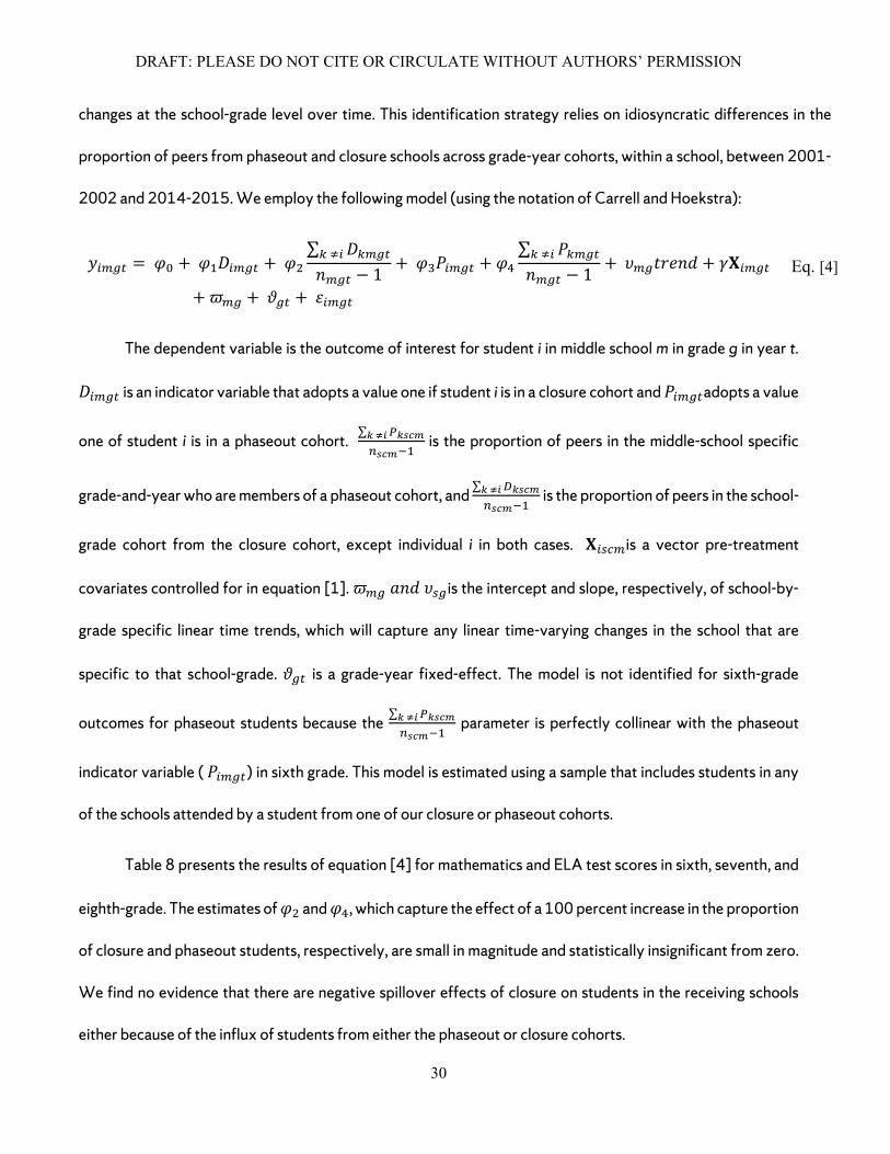
𝑦𝑦𝑖𝑖𝑖𝑖𝑖𝑖𝑖𝑖 = 𝜑𝜑0 + 𝜑𝜑1𝐷𝐷𝑖𝑖𝑖𝑖𝑖𝑖𝑖𝑖 + 𝜑𝜑2∑ 𝐷𝐷𝑘𝑘𝑖𝑖𝑖𝑖𝑖𝑖𝑘𝑘 ≠𝑖𝑖
𝑛𝑛𝑖𝑖𝑖𝑖𝑖𝑖 − 1+ 𝜑𝜑3𝑃𝑃𝑖𝑖𝑖𝑖𝑖𝑖𝑖𝑖 + 𝜑𝜑4
∑ 𝑃𝑃𝑘𝑘𝑖𝑖𝑖𝑖𝑖𝑖𝑘𝑘 ≠𝑖𝑖
𝑛𝑛𝑖𝑖𝑖𝑖𝑖𝑖 − 1+ 𝜐𝜐𝑖𝑖𝑖𝑖𝑡𝑡𝑡𝑡𝑡𝑡𝑛𝑛𝑡𝑡 + 𝛾𝛾𝚾𝚾𝑖𝑖𝑖𝑖𝑖𝑖𝑖𝑖
+ 𝜛𝜛𝑖𝑖𝑖𝑖 + 𝜗𝜗𝑖𝑖𝑖𝑖 + 𝜀𝜀𝑖𝑖𝑖𝑖𝑖𝑖𝑖𝑖
The dependent variable is the outcome of interest for student i in middle school m in grade g in year t.
𝐷𝐷𝑖𝑖𝑖𝑖𝑖𝑖𝑖𝑖 is an indicator variable that adopts a value one if student i is in a closure cohort and 𝑃𝑃𝑖𝑖𝑖𝑖𝑖𝑖𝑖𝑖adopts a value
one of student i is in a phaseout cohort. ∑ 𝑃𝑃𝑘𝑘𝑘𝑘𝑘𝑘𝑘𝑘𝑘𝑘 ≠𝑖𝑖𝑛𝑛𝑘𝑘𝑘𝑘𝑘𝑘−1
is the proportion of peers in the middle-school specific
grade-and-year who are members of a phaseout cohort, and ∑ 𝐷𝐷𝑘𝑘𝑘𝑘𝑘𝑘𝑘𝑘𝑘𝑘 ≠𝑖𝑖𝑛𝑛𝑘𝑘𝑘𝑘𝑘𝑘−1
is the proportion of peers in the school-
grade cohort from the closure cohort, except individual i in both cases. 𝚾𝚾𝑖𝑖𝑖𝑖𝑖𝑖𝑖𝑖is a vector pre-treatment
covariates controlled for in equation [1]. 𝜛𝜛𝑖𝑖𝑖𝑖 𝑎𝑎𝑛𝑛𝑡𝑡 𝜐𝜐𝑖𝑖𝑖𝑖is the intercept and slope, respectively, of school-by-
grade specific linear time trends, which will capture any linear time-varying changes in the school that are
specific to that school-grade. 𝜗𝜗𝑖𝑖𝑖𝑖 is a grade-year fixed-effect. The model is not identified for sixth-grade
outcomes for phaseout students because the ∑ 𝑃𝑃𝑘𝑘𝑘𝑘𝑘𝑘𝑘𝑘𝑘𝑘 ≠𝑖𝑖𝑛𝑛𝑘𝑘𝑘𝑘𝑘𝑘−1
parameter is perfectly collinear with the phaseout
indicator variable ( 𝑃𝑃𝑖𝑖𝑖𝑖𝑖𝑖𝑖𝑖) in sixth grade. This model is estimated using a sample that includes students in any
of the schools attended by a student from one of our closure or phaseout cohorts.
Table 8 presents the results of equation [4] for mathematics and ELA test scores in sixth, seventh, and
eighth-grade. The estimates of 𝜑𝜑2 and 𝜑𝜑4, which capture the effect of a 100 percent increase in the proportion
of closure and phaseout students, respectively, are small in magnitude and statistically insignificant from zero.
We find no evidence that there are negative spillover effects of closure on students in the receiving schools
either because of the influx of students from either the phaseout or closure cohorts.
Eq. [4]
DRAFT: PLEASE DO NOT CITE OR CIRCULATE WITHOUT AUTHORS’ PERMISSION
31
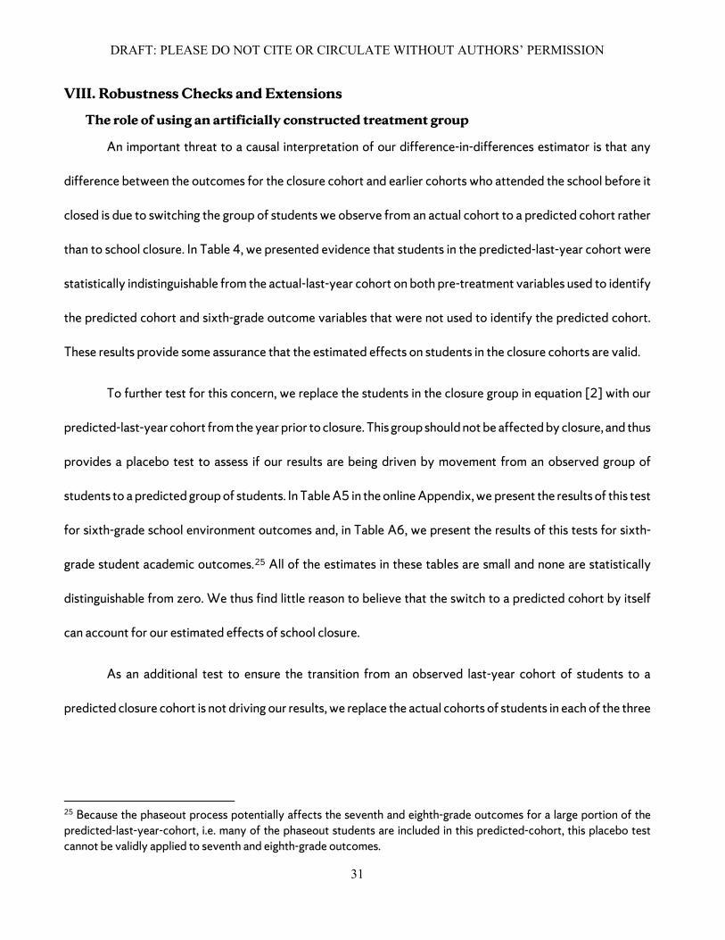
VIII. Robustness Checks and Extensions
The role of using an artificially constructed treatment group
An important threat to a causal interpretation of our difference-in-differences estimator is that any
difference between the outcomes for the closure cohort and earlier cohorts who attended the school before it
closed is due to switching the group of students we observe from an actual cohort to a predicted cohort rather
than to school closure. In Table 4, we presented evidence that students in the predicted-last-year cohort were
statistically indistinguishable from the actual-last-year cohort on both pre-treatment variables used to identify
the predicted cohort and sixth-grade outcome variables that were not used to identify the predicted cohort.
These results provide some assurance that the estimated effects on students in the closure cohorts are valid.
To further test for this concern, we replace the students in the closure group in equation [2] with our
predicted-last-year cohort from the year prior to closure. This group should not be affected by closure, and thus
provides a placebo test to assess if our results are being driven by movement from an observed group of
students to a predicted group of students. In Table A5 in the online Appendix, we present the results of this test
for sixth-grade school environment outcomes and, in Table A6, we present the results of this tests for sixth-
grade student academic outcomes.25 All of the estimates in these tables are small and none are statistically
distinguishable from zero. We thus find little reason to believe that the switch to a predicted cohort by itself
can account for our estimated effects of school closure.
As an additional test to ensure the transition from an observed last-year cohort of students to a
predicted closure cohort is not driving our results, we replace the actual cohorts of students in each of the three
25 Because the phaseout process potentially affects the seventh and eighth-grade outcomes for a large portion of the predicted-last-year-cohort, i.e. many of the phaseout students are included in this predicted-cohort, this placebo test cannot be validly applied to seventh and eighth-grade outcomes.

DRAFT: PLEASE DO NOT CITE OR CIRCULATE WITHOUT AUTHORS’ PERMISSION
32
years prior to closure with predicted cohorts of students in each year.26 We then estimate equation [2] using
only predicted cohorts. These estimates can be interpreted as the effect of school closure on students likely to
have attended a closed school and cannot be contaminated by a switch from actual to predicted cohorts.
The top panel of Table 9 presents the effects of closure on the school environment for each student
based on their pre-treatment quintile of fifth-grade math performance. Our results are consistent with the
effects found using the main model (see Table 5), albeit slightly smaller in magnitude and slightly less precisely
estimated. We continue to find evidence that the top quintile of students in the closure cohort attends
systematically different schools as a result of closure. While the magnitudes are slightly smaller, closure induced
the top quintile of students to attend schools that performed 0.077 standard deviations better on school-level
sixth-grade math, 0.084 standard deviations higher in terms of value-added, and travel 0.132 miles farther to
attend the school than similar high performers in previous cohorts.
The bottom panel of Table 9 presents the effects of closure on student outcomes estimated using the
full predicted-cohort sample. Consistent with the results from our primary analysis presented in Table 7, we
find closure caused students in the top quintile to perform measurably better on their sixth, seventh, and eighth-
grade math exams. These effect estimates are similar in magnitude to the corresponding estimates in Table 7,
and statistically significant. The effects on absentee rates are also qualitatively similar to those found in our
primary model. Table 9 provides compelling evidence that the estimated effects of closure on high-performing
26 All predicted cohorts are constructed using the same strategy that we used to identify students in our closure cohorts. For schools that closed in 2004-05, the cohort for three-years prior to closure (AY 2002-03) is estimated using only one year of data as opposed to two. However, there were no systematic differences in the overall accuracy or treatment coverage rates for this cohort relative to any other cohort. Our treatment coverage and accuracy rates are consistent with those in Table 3 for all years prior to closure.

DRAFT: PLEASE DO NOT CITE OR CIRCULATE WITHOUT AUTHORS’ PERMISSION
33
students found in the primary model are not being driven by moving from an actual cohort of students to a
predicted cohort of students.27
The role school quality?
Lastly, we consider the extent to which the effect of closure varies by the quality of the receiving
school. To examine this question, we split each treatment variable into two. Specifically, we replace the
treatment indicators in equation [2], 𝐷𝐷𝑖𝑖𝑖𝑖 and 𝑃𝑃𝑖𝑖𝑖𝑖 , with a set of binary variables that indicate, respectively, that
a student (a) is in a closure cohort and entered sixth grade in a school with a lagged value-added measure
greater than the city average, (b) is in a closure cohort and entered sixth grade in a school with a lagged value-
added measure below the city average, (c) is in phaseout cohort and in the first year following closure attended
a school with a lagged value-added measures greater than the city average, and (d) is in a phaseout cohort and
in the first year following closure attended a school with a lagged value-added measure less than the city wide
average. We estimated each model separately for each quintile of students defined by performance on the fifth
grade math test.
It is important to note that the quality of the school a student chooses to attend is an endogenous choice
and is likely to be correlated with unobserved student characteristics. Thus, estimates of how effects of school
closure vary by the quality of the schools that a student attends after the closing cannot be interpreted causally,
even if we accept the assumptions of our strategy for identifying the average effects of school closure. The
results of this model should be interpreted as merely additional suggestive evidence about the role school
quality changes play in mediating school closure effects.
27 We also estimate equation [3] using only predicted cohorts in all years, including pre-treatment years. We find that there are no statistical or substantive changes from the results we present in Figure 4 or Appendix Table 1.

DRAFT: PLEASE DO NOT CITE OR CIRCULATE WITHOUT AUTHORS’ PERMISSION
34
The results are presented in Table 10. Whether effects vary by the value-added of the school a student
entered after closure can be discerned by comparing columns (1) and (2), and columns (3) and (4). In each
case, the effect of school closure is more positive if the student affected by closure attends a school with higher
value-added the year following closure. None of the differences in the effects of sorting to an above average
value-added school and sorting to a below average value-added school are statistically significant, and so we
must be careful not to over-interpret these results. However, the fact that effects are always more positive
when students attend a school with above average value-added than when they attend schools with below
average value-added suggests that the effects of school closure depend on the quality of alternatives available
to students and those chosen by students who otherwise would be relegated to the school that closed.
The last column of Table 10 indicates that higher achieving students are considerably more likely to
attend schools with relatively high value-added in response to closure. This fact, combined with the finding that
the effects of closure are positive and statistically significant only for relatively high-achieving students in the
closure cohorts who attend schools with above average value-added, suggests that the quality of schools
attended in response to closure plays some role in explaining why high-achieving students benefit more from
school closure than low achieving students. However, the effects of closure on low-achieving students in the
closure cohorts are close to zero even when those students select into relatively high value-added school, which
suggests that school quality is not the only factor influencing the effects of school quality.
A final noteworthy aspect of the results in Table 10 is that, although the estimated effects of school
closure on the achievement of students in the phaseout cohorts are statistically significant only for low-
performing students who attend schools with below average value-added, virtually all of the point estimates of
the effects on phaseout students are negative. Point estimates are negative even when students transfer to
schools with above average value-added. These results suggest that both the degradation in school quality at

DRAFT: PLEASE DO NOT CITE OR CIRCULATE WITHOUT AUTHORS’ PERMISSION
35
schools designated for closure and the disruption effects that accompany changing middle schools mid-stream,
make it difficult to extend potential benefits of school closure to students who attend the school at the time of
closure, at least in the short-term.
IX. Conclusions
Prior literature on school closure has largely focused on identifying the effects of closure on students
who were attending a closed school when it closed and on students in schools receiving students from closed
schools. This literature has also tended to comingle school closure due to declining enrollments with closures
due to low-performance. In this paper, we estimate effects of accountability-driven middle school closures in
New York City on students who likely would have entered a closed school had it not closed, as well as on
students attending the closed school when closure is initiated. The effects of disruption often associated with
school closures are likely to be much smaller for the former group than the latter group. Also, we examine how
the effects of closure on both sets of students vary across students with different fifth-grade achievement
levels.
We find that accountability-driven closure induced higher-achieving students in the post-closure
cohorts to attend higher-performing schools with more white students and fewer students eligible for free-and-
reduced-price lunch. We also find these students performed better on tests of math and English language arts
beginning in sixth grade as a result of closure and that these positive effects lasted through eighth grade. In
contrast, lower-performing students in these post-closure cohorts enrolled in middle schools that are similar to
the closed school in terms of demographics and achievement, and, on average, these students did not see
improvement in their test scores as a result of closure. These results were found for multiple cohorts following
closure and are robust to several threats to internal validity that we considered. Both this pattern of results, and
analyses that attempt to estimate the extent to which changes in school quality mediate the effect of school

DRAFT: PLEASE DO NOT CITE OR CIRCULATE WITHOUT AUTHORS’ PERMISSION
36
closure, suggests that the quality of school that students attend following closure has important implications
for what effect closure is likely to have.
We also find that among the students who were already attending the closed school when the phaseout
process was initiated, the relatively high-achieving students were more likely to transfer out of the school than
low-achieving students. We also find that school closure had negative effects on the low-performing students
in these phaseout cohorts.
These results suggest at least two important policy implications. The first is that providing high-quality
alternatives to students who otherwise would attend closed schools may be necessary for school closures to
have positive effects on student achievement. An examination of the system for assigning students to middle
school in effect at the time of the school closures we examine suggests that low-achieving students typically
had fewer middle school options available to them than high-achieving students. Also, the pattern of results
suggests that this difference in accessible alternatives may be part of the reason why high-performing students
benefitted more from school closure than lower-performing students.
Second, our results indicate that school closure decisions present important tradeoffs. Our results
indicate that school closure can benefit at least some students in future cohorts, particularly if those students
have high-quality alternatives available to them. However, these gains for future cohorts might come at the
expense of worse outcomes for students currently in the schools slated for closure. Our findings concerning
the effects on students currently in a school designated for closure pertain to the closure policy implemented
in New York City, under which a large proportion of students remain in the school designated for closure during
a phaseout period. Our evidence suggests that in such a case, particularly when transfer options for students in
schools designated for closure are limited, students in these closed schools are made worse off. Although our
evidence cannot speak directly to the effects of a policy that would close schools all at once, forcing students

DRAFT: PLEASE DO NOT CITE OR CIRCULATE WITHOUT AUTHORS’ PERMISSION
37
to transfer immediately, evidence from other studies suggest such policies can also create negative disruption
effects for students currently attending a school designated for closure (de la Torre and Gwynne 2009;
Engberg et al. 2012; Kirshner, Gaertner, and Pozzoboni 2010; Ozek, Hansen, and Gonzalez 2012). Thus,
although this study cannot provide guidance on whether phaseout policies like the one deployed in New York
City or all-at-once closures are likely to be better for students currently attending the school, our results do
suggest that avoiding negative impacts on this group of students can be difficult.
Assessing the potential gains to future cohorts relative to the potential losses to current students
requires value judgments by policymakers. It is tempting to say that gains to future cohorts can accrue over
many years and thus for many cohorts while any losses to current students will be limited to a smaller number
of cohorts, and thus, the gains are likely to justify the losses. However, in the case of New York City, it appears
that gains for future cohorts were limited to students who were already relatively high achieving, while losses
accrued to lower-performing students in the phaseout cohorts. Such considerations complicate the
assessment. It might be in a context where both low and high-achieving students in both the future and current
cohorts were given access to high-quality alternatives, school closures would result in a more equitable
distribution of benefits. However, in most contexts, unequivocally positive effects are likely to be difficult to
realize, so policymakers will have to pay careful attention to tradeoffs like the ones highlighted in this study.

DRAFT: PLEASE DO NOT CITE OR CIRCULATE WITHOUT AUTHORS’ PERMISSION
38
Work Cited:
Abdulkadiroglu, A., Angirst, J. D., , Hull, P. D., & Pathak, P. A. Pathak. 2016. Charters Without Lotteries: Testing Takeovers in New Orleans and Boston. American Economic Review. 106.7, 1878-1920.
Capps, R., Fix, M., Murray, J., Ost, J., Passel, J.S., & Herwantoro, S. 2005. The new demography of America's schools: Immigration and the No Child Left Behind Act. Urban Institute (NJ1).
Carlson, D. & Lavertu, S. 2016. Charter school closure and student achievement: Evidence from Ohio. Journal of Urban Economics, 95, 31-48.
Carrell, S. E., & Hoekstra, M. L. 2010. Externalities in the Classroom: How Children Exposed to Domestic Violence Affect Everyone's Kids. American Economic Journal: Applied Economics. 2, 211-228.
Center for Research on Education Outcomes (CREDO). 2017. Lights Off: Practice and Impact of Closing Low-Performing schools. Stanford, CA: CREDO.
Brummet, Q. 2014. The effect of school closings on student achievement. Journal of Public Economics. 119, 108-124.
Bross, W., Harris Douglas N., & Lihan L. 2016. The Effects of Performance-Based Closure and Charter Takeover on Student Performance. New Orleans: Education Research Alliance for New Orleans.
De la Torre, M. & Gwynne J. 2009. When Schools Close: Effects on Displaced Students in Chicago Public Schools. Chicago: Consortium on Chicago School Research at the University of Chicago.
De la Torre, M., Gordon, M. F., Moore, P., & Cowhy, J. 2015. School Closings in Chicago: Understanding Families' Choices and Constraints for New School Enrollment. Chicago: Consortium on Chicago School Research at the University of Chicago.
Engberg, J., Gill, B., Zamarro, G., & Zimmer, R. 2012. Closing schools in a shrinking district: Do student outcomes depend on which schools are closed? Journal of Urban Economics, 71(2), 189-203.
Ehlert, M., Koedel, C., Parson, E. & Podgursky, M. J. 2012. Selection Growth Models for Schools and Teacher Evaluations. National Center for Analysis of Longitudinal Data in Education (CALDER) Working Paper, No. 80.
Ehlert, M., Koedel, C., Parson, E. & Podgursky, M. J. 2014. The Sensitivity of Value-Added Estimates to Specification Adjustments: Evidence From School- and Teacher-Level Models in Missouri. Statistics and Public Policy, 1(1), 19-27.
Figlio, D. N., & Rouse, C. E. 2006. Do accountability and voucher threats improve low-performing schools? Journal of Public Economics. 90, 239-255.
Hoxby, C. M., Sonali M., & Kang, J. 2009. How New York City’s charter schools affect achievement. Cambridge, MA: New York City Charter Schools Evaluation Project, 1-85.

DRAFT: PLEASE DO NOT CITE OR CIRCULATE WITHOUT AUTHORS’ PERMISSION
39
Hanushek, E. A., Kain, J. F., & Rivkin, S. G. 2004. Disruption Versus Tiebout Improvement: the Costs and Benefits of Switching Schools. Journal of Public Economics. 88, 1721-1746.
Imbens, G. W. & Rubin, D. B. 2015. Causal Inference for Statistics, Social, and Biomedical Sciences an Introduction. Cambridge: Cambridge University Press.
Kemple, J. 2015. High School Closures in New York City. The Research Alliance for New York City Schools.
Krishner, B., Gaertner, M., & Pozzoboni, K. 2010. Tracing transitions: the effects of high school closure on displaced students. Education Evaluation and Policy Analysis. 32(3), 407-429.
Michelmore, K. & Dynarski, S. 2017. The Gap Within the Gap: Using Longitudinal Data to Understand Income Differences in Educational Outcomes. AERA Open. 3(1).
Özek, U., Hansen, M. Hansen, & Gonzalez, T. 2012. A Leg Up or a Boot Out? Student achievement and mobility under school restricting. Washington, D.C.: National Center for Analysis of Longitudinal Data in Education Research.
Rockoff, J. & Turner, L. J. 2010. Short-Run Impacts of Accountability on School Quality. American Economic Journal Economic Policy. 2(4), 119-147.
Steiner, L. 2009. Tough Decisions: Closing Persistently Low-Performing Schools. Lincoln, NE: Academic Development Institute.
Strunk, K. O., Marsh, J. A., Hashim, A. K., Bush-Mecenas, S., & Weinstein, T. 2016. The Impact of Turnaround Reform on Student Outcomes: Evidence and Insights from the Los Angeles Unified School District. Education Finance and Policy. 11(3), 251-282.
Sunderman, G. L. & Payne, A. 2009. Does Closing Schools Cause Educational Harm? A Review of the Research. Information Brief.

DRAFT: PLEASE DO NOT CITE OR CIRCULATE WITHOUT AUTHORS’ PERMISSION
40
Figure 1.
6th Graders who would have attended a Closed School as a Percent of Sixth-Grade Cohort in Receiving Schools
7th and 8th Graders from Phaseout Schools as a Percent of 7th and 8th Graders in Receiving Schools
Mean (5.18%)
Median (4.08%)
020
040
060
080
0N
umbe
r of S
choo
l-Yea
r Obs
erva
tions
0 .1 .2 .3Sixth Graders who would have attended a Closed School as a Percent of Sixth-Grade Cohort in Receiving School
Distribution of Students from Closed Schools
Median (2.67%)
Mean (3.17%)
010
2030
4050
Num
ber o
f Sch
ool-Y
ear O
bser
vatio
ns
0 .02 .04 .06 .08 .17th and 8th Graders from Phaseout as a Percent of 7th and 8th Graders in Schools
Distribution of Students from Closed Schools

DRAFT: PLEASE DO NOT CITE OR CIRCULATE WITHOUT AUTHORS’ PERMISSION
41
Figure 2: Causal Pathway between School Closure and Student Performance

DRAFT: PLEASE DO NOT CITE OR CIRCULATE WITHOUT AUTHORS’ PERMISSION
42
Figure 3: Estimates of Difference in Pre-Closure Trends on Key Sixth-Grade Outcomes
School-Level Sixth-Grade ELA School-Level Sixth-Grade Math School-Level Value-Added
School-Level Distance Traveled Student-Level Sixth-Grade ELA Student-Level Sixth-Grade Math

DRAFT: PLEASE DO NOT CITE OR CIRCULATE WITHOUT AUTHORS’ PERMISSION
43
Figure 4: Event Study Results for Top Quintile StudentsA
Mathematics Scores in Sixth Grade Mathematics Scores in Eighth Grade
ELA Scores in Sixth Grade ELA Scores in Eighth Grade
Notes: (a) top quintiles are students scoring in top quintile of their school’s 5th grade mathematics exam
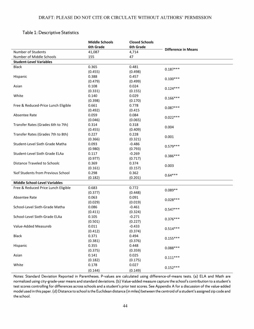
DRAFT: PLEASE DO NOT CITE OR CIRCULATE WITHOUT AUTHORS’ PERMISSION
44
Table 1: Descriptive Statistics
Middle Schools 6th Grade
Closed Schools 6th Grade
Difference in Means Number of Students 41,087 4,714 Number of Middle Schools 155 47 Student-Level Variables Black 0.365 0.481 0.187*** (0.455) (0.498) Hispanic 0.388 0.457 0.100*** (0.479) (0.499) Asian 0.108 0.024 0.124*** (0.331) (0.155) White 0.140 0.029 0.166*** (0.398) (0.170) Free & Reduced-Price Lunch Eligible 0.661 0.778 0.087*** (0.492) (0.415 Absentee Rate 0.059 0.084 0.022*** (0.046) (0.065) Transfer Rates (Grades 6th to 7th) 0.314 0.318 0.004 (0.455) (0.409) Transfer Rates (Grades 7th to 8th) 0.227 0.228 0.001 (0.366) (0.321) Student-Level Sixth Grade Matha 0.093 -0.486 0.579*** (0.980) (0.793) Student-Level Sixth Grade ELAa 0.117 -0.269 0.386*** (0.977) (0.717) Distance Traveled to Schoolc 0.369 0.374 0.003 (0.161) (0.157) %of Students from Previous School 0.298 0.362 0.64*** (0.182) (0.201) Middle School-Level Variables Free & Reduced Price Lunch Eligible 0.683 0.772 0.089** (0.377) (0.448) Absentee Rate 0.063 0.091 0.028*** (0.029) (0.019) School-Level Sixth-Grade Matha 0.086 -0.461 0.547*** (0.411) (0.324) School-Level Sixth-Grade ELAa 0.105 -0.271 0.376*** (0.501) (0.227) Value-Added Measureb 0.011 -0.433 0.514*** (0.412) (0.374) Black 0.371 0.494 0.155*** (0.381) (0.376) Hispanic 0.355 0.448 0.088*** (0.375) (0.359) Asian 0.141 0.025 0.111*** (0.182) (0.175) White 0.178 0.027
0.152*** (0.144) (0.149) Notes: Standard Deviation Reported in Parentheses. P-values are calculated using difference-of-means tests. (a) ELA and Math are normalized using city-grade-year means and standard deviations. (b) Value-added measure capture the school’s contribution to a student’s test scores controlling for differences across schools and a student’s prior test scores. See Appendix A for a discussion of the value-added model used in this paper. (d) Distance to school is the Euclidean distance (in miles) between the centroid of a student's assigned zip code and the school.

DRAFT: PLEASE DO NOT CITE OR CIRCULATE WITHOUT AUTHORS’ PERMISSION
45
Table 2: Are Later Closures a Good Comparison for Early Closures?
(1) (2) (3) (4) (5) (6) (7) (8) Year of School Closure 2004-05 2005-06 2006-07 2007-08 2008-09 2009-10 2010-11 2011-12 Number of Closed Schools by Year 9 5 3 8 2 3 1 15 Schools that have not yet Closed 38 33 30 22 20 17 16 1 Difference of Means School-Level Sixth-Grade ELA Performance
0.001 0.006 0.001 0.002 0.002 0.001 0.004 0.015
School-Level Sixth-Grade Math Performance
0.010 0.002 0.016 0.003 0.007 0.001 0.016 0.035
School-Level Value Addeda 0.008 0.008 0.007 0.002 0.006 0.002 0.008 0.014 Percent Black 0.030 0.030 0.018 0.010 0.010 0.010 0.010 0.050 Percent Hispanic 0.030 0.020 0.010 0.010 0.020 0.020 0.010 0.034 Absentee Rate 0.010 0.010 0.010 0.021 0.010 0.010 0.020 0.000 Percent Free-and-Reduced-Price-Lunch Eligible
0.005 0.005 0.002 0.012 0.002 0.001 0.009 0.003
Percent English Lang. Learner 0.001 0.001 0.013 0.011 0.004 0.010 0.008 0.018
Note: This table summarizes difference of means on school-level covariates between schools that closed in each given year (based on data from the year prior to closure) to schools that have not yet closed but will closed by the 2012-2013 academic year. Differences of means tests were conducted. ***p<0.01, **p<0.05, *p<0.10. ELA and Math are normalized using city-grade-year means and standard deviations. (a) See Table 1 and appendix A for a description of our value-added measure.

DRAFT: PLEASE DO NOT CITE OR CIRCULATE WITHOUT AUTHORS’ PERMISSION
46
Table 3: Accuracy and Treatment Coverage Rates of our Matching Strategy
School ID Phaseout Year True Last Year Cohort
Predicted Last Year Cohort
Accuracy Rate Treatment Coverage Rate
All Closed Schools
All Years 4078 3599 74% 66%
098456 2004-05 120 98 73% 60% 042274 2004-05 61 52 71% 61% 020129 2004-05 56 48 73% 63% 001895 2004-05 287 206 70% 50% 011205 2004-05 210 207 74% 73% 082138 2004-05 293 231 76% 60% 053442 2004-05 396 329 77% 64% 031081 2004-05 62 53 68% 58% 046463 2004-05 321 303 68% 64% 000501 2005-06 31 30 67% 65% 006676 2005-06 284 241 76% 65% 038548 2005-06 118 115 75% 73% 037068 2005-06 113 93 75% 62% 064464 2005-06 276 274 78% 78% 049543 2006-07 57 57 79% 79% 004502 2006-07 50 44 73% 64% 043284 2006-07 74 72 86% 84% 085812 2007-08 27 26 62% 59% 031190 2007-08 108 71 69% 45% 025985 2007-08 54 54 70% 70% 093212 2007-08 118 113 73% 70% 002563 2007-08 108 92 75% 64% 051952 2007-08 104 100 77% 74% 014482 2007-08 25 17 59% 40% 051434 2007-08 123 109 77% 68% 075126 2008-09 61 61 79% 79% 015074 2008-09 132 109 68% 56% 077648 2009-10 67 67 66% 66% 085740 2009-10 75 70 77% 72% 065270 2009-10 232 223 80% 77% 013668 2010-11 35 34 74% 71%
Notes: The accuracy rate is the percentage of the predicted-last-year cohort members that are in the actual-last-year cohort. The treatment coverage rate is the percentage of students in the actual-last-year cohort who are also in the predicted-last-year cohort.

DRAFT: PLEASE DO NOT CITE OR CIRCULATE WITHOUT AUTHORS’ PERMISSION
47
Table 4: Comparing the Last-Year Actual and Predicted-Cohort Students
(1) Column (2) Variable Last-Year Cohort Predicted-Last-Year
Cohort Fifth Grade Variables Percent Blacka 0.477 0.482 Percent Hispanica 0.454 0.451 Percent Asiana 0.025 0.027 Percent Whitea 0.043 0.044 Percent Free-and-Reduced-Price Lunch Eligiblea 0.778 0.772 Student-Level Fifth-Grade Absentee Rate 0.081 0.079 Student-Level Fifth-Grade English -0.254 -0.249 Student-Level Fifth-Grade Math -0.471 -0.469 Sixth-Grade Outcomes School-Level Sixth Grade Mathb -0.462 -0.448 School-Level Sixth Grade Englishb -0.259 -0.247 School-Level Sixth-Grade Value-Addedc -0.671 -0.654 Distance Traveled (Sixth Grade)d 0.364 0.368 Student-Level Sixth-Grade English -0.262 -0.257 Student-Level Sixth-Grade Math -0.471 -0.464 Student-Level Sixth-Grade Absentee Rate 0.096 0.088
Notes: The Last-Year Cohort consists of all students who attended a closed school in the year prior to phaseout beginning. The Predicted-Last-Year cohort consists of students that we predict as attending the school in the last year prior to closure. Means are reported for each group for each variable. Simple difference of means tests between each group and the last-year cohort were conducted and none of the differences are statistically significant at the 0.10 level. (a) Racial and socioeconomic variables are measured prior to treatment (reported race in fifth-grade. All English and math performance data is normalized at the city-grade-year level. (b) ELA and Math are normalized using city-grade-year means and standard deviations. (c)Value-added measure capture the school’s contribution to a student’s test scores controlling for differences across schools and a student’s prior test scores. See Appendix A for a discussion of the value-added model used in this paper. (d) Distance to school is the Euclidean distance (in miles) between the centroid of a student's assigned zip code and the school.
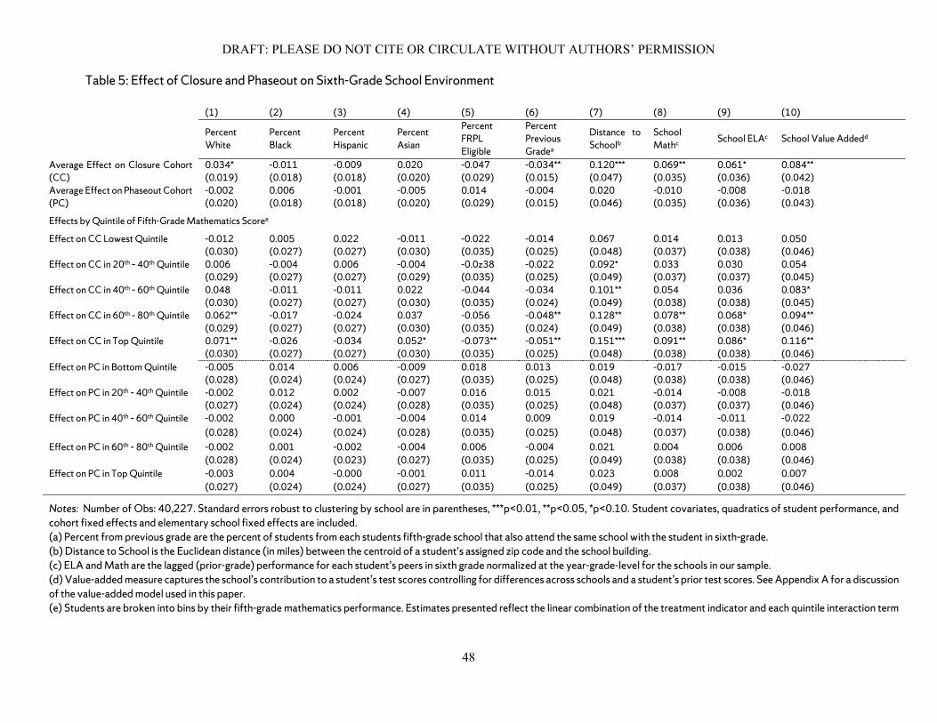
DRAFT: PLEASE DO NOT CITE OR CIRCULATE WITHOUT AUTHORS’ PERMISSION
48
Table 5: Effect of Closure and Phaseout on Sixth-Grade School Environment
(1) (2) (3) (4) (5) (6) (7) (8) (9) (10)
Percent White
Percent Black
Percent Hispanic
Percent Asian
Percent FRPL Eligible
Percent Previous Gradea
Distance to Schoolb
School Mathc School ELAc School Value Addedd
Average Effect on Closure Cohort (CC)
0.034* -0.011 -0.009 0.020 -0.047 -0.034** 0.120*** 0.069** 0.061* 0.084** (0.019) (0.018) (0.018) (0.020) (0.029) (0.015) (0.047) (0.035) (0.036) (0.042)
Average Effect on Phaseout Cohort (PC)
-0.002 0.006 -0.001 -0.005 0.014 -0.004 0.020 -0.010 -0.008 -0.018 (0.020) (0.018) (0.018) (0.020) (0.029) (0.015) (0.046) (0.035) (0.036) (0.043)
Effects by Quintile of Fifth-Grade Mathematics Scoree
Effect on CC Lowest Quintile -0.012 0.005 0.022 -0.011 -0.022 -0.014 0.067 0.014 0.013 0.050 (0.030) (0.027) (0.027) (0.030) (0.035) (0.025) (0.048) (0.037) (0.038) (0.046) Effect on CC in 20th – 40th Quintile 0.006 -0.004 0.006 -0.004 -0.0z38 -0.022 0.092* 0.033 0.030 0.054 (0.029) (0.027) (0.027) (0.029) (0.035) (0.025) (0.049) (0.037) (0.037) (0.045) Effect on CC in 40th – 60th Quintile 0.048 -0.011 -0.011 0.022 -0.044 -0.034 0.101** 0.054 0.036 0.083* (0.030) (0.027) (0.027) (0.030) (0.035) (0.024) (0.049) (0.038) (0.038) (0.045) Effect on CC in 60th – 80th Quintile 0.062** -0.017 -0.024 0.037 -0.056 -0.048** 0.128** 0.078** 0.068* 0.094** (0.029) (0.027) (0.027) (0.030) (0.035) (0.024) (0.049) (0.038) (0.038) (0.046) Effect on CC in Top Quintile 0.071** -0.026 -0.034 0.052* -0.073** -0.051** 0.151*** 0.091** 0.086* 0.116** (0.030) (0.027) (0.027) (0.030) (0.035) (0.025) (0.048) (0.038) (0.038) (0.046) Effect on PC in Bottom Quintile -0.005 0.014 0.006 -0.009 0.018 0.013 0.019 -0.017 -0.015 -0.027 (0.028) (0.024) (0.024) (0.027) (0.035) (0.025) (0.048) (0.038) (0.038) (0.046) Effect on PC in 20th – 40th Quintile -0.002 0.012 0.002 -0.007 0.016 0.015 0.021 -0.014 -0.008 -0.018 (0.027) (0.024) (0.024) (0.028) (0.035) (0.025) (0.048) (0.037) (0.037) (0.046) Effect on PC in 40th – 60th Quintile -0.002 0.000 -0.001 -0.004 0.014 0.009 0.019 -0.014 -0.011 -0.022 (0.028) (0.024) (0.024) (0.028) (0.035) (0.025) (0.048) (0.037) (0.038) (0.046) Effect on PC in 60th – 80th Quintile -0.002 0.001 -0.002 -0.004 0.006 -0.004 0.021 0.004 0.006 0.008 (0.028) (0.024) (0.023) (0.027) (0.035) (0.025) (0.049) (0.038) (0.038) (0.046) Effect on PC in Top Quintile -0.003 0.004 -0.000 -0.001 0.011 -0.014 0.023 0.008 0.002 0.007 (0.027) (0.024) (0.024) (0.027) (0.035) (0.025) (0.049) (0.037) (0.038) (0.046)
Notes: Number of Obs: 40,227. Standard errors robust to clustering by school are in parentheses, ***p<0.01, **p<0.05, *p<0.10. Student covariates, quadratics of student performance, and cohort fixed effects and elementary school fixed effects are included. (a) Percent from previous grade are the percent of students from each students fifth-grade school that also attend the same school with the student in sixth-grade. (b) Distance to School is the Euclidean distance (in miles) between the centroid of a student's assigned zip code and the school building. (c) ELA and Math are the lagged (prior-grade) performance for each student’s peers in sixth grade normalized at the year-grade-level for the schools in our sample. (d) Value-added measure captures the school’s contribution to a student’s test scores controlling for differences across schools and a student’s prior test scores. See Appendix A for a discussion of the value-added model used in this paper. (e) Students are broken into bins by their fifth-grade mathematics performance. Estimates presented reflect the linear combination of the treatment indicator and each quintile interaction term
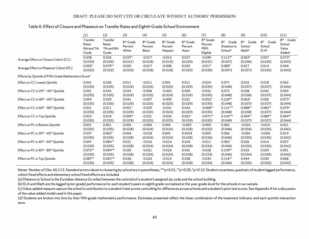
DRAFT: PLEASE DO NOT CITE OR CIRCULATE WITHOUT AUTHORS’ PERMISSION
49
Table 6: Effect of Closure and Phaseout on Transfer Rates and Eighth-Grade School Environment
(1) (2) (3) (4) (5) (6) (7) (8) (9) (10) (11)
Transfer Rates 6th and 7th Grade
Transfer Rates 7th and 8th Grade
8th Grade Percent White
8th Grade Percent Black
8th Grade Percent Hispanic
8th Grade Percent Asian
8th Grade Percent FRPL Eligible
8th Grade Distance to Schoola
8th Grade School Mathb
8th Grade School ELAb
8th Grade School Value Addedc
Average Effect on Closure Cohort (CC) 0.038 0.026 0.037* -0.017 -0.014 0.027 -0.049 0.112** 0.062* 0.057 0.073* (0.033) (0.034) (0.021) (0.018) (0.019) (0.020) (0.031) (0.047) (0.036) (0.035) (0.043)
Average Effect on Phaseout Cohort (PC) 0.055* 0.079** 0.020 -0.017 -0.008 0.025 -0.017 0.085* 0.017 0.014 0.040 (0.032) (0.032) (0.020) (0.018) (0.018) (0.020) (0.030) (0.047) (0.037) (0.035) (0.043)
Effects by Quintile of Fifth-Grade Mathematics Scored
Effect on CC Lowest Quintile 0.041 0.036 0.011 -0.011 0.001 0.011 -0.024 0.071 0.025 0.018 0.042 (0.035) (0.035) (0.029) (0.024) (0.024) (0.029) (0.035) (0.048) (0.037) (0.037) (0.044) Effect on CC in 20th – 40th Quintile 0.051 0.034 0.024 -0.006 -0.003 0.009 -0.032 0.072 0.038 0.042 0.059 (0.035) (0.035) (0.029) (0.025) (0.024) (0.029) (0.035) (0.048) (0.038) (0.037) (0.044) Effect on CC in 40th – 60th Quintile 0.054 0.029 0.041 -0.007 -0.009 0.021 -0.052* 0.120** 0.063* 0.056 0.073* (0.035) (0.035) (0.029) (0.025) (0.025) (0.029) (0.035) (0.048) (0.037) (0.037) (0.044) Effect on CC in 60th – 80th Quintile 0.021 0.011 0.051* -0.029 -0.031 0.044 -0.068** 0.131*** 0.088** 0.082** 0.079* (0.035) (0.035) (0.029) (0.025) (0.024) (0.029) (0.035) (0.048) (0.038) (0.037) (0.044) Effect on CC in Top Quintile 0.023 0.018 0.059** -0.031 -0.026 0.051* -0.071** 0.143*** 0.094** 0.089** 0.094** (0.035) (0.035) (0.029) (0.025) (0.025) (0.029) (0.035) (0.048) (0.037) (0.037) (0.044) Effect on PC in Bottom Quintile 0.031 0.051 0.004 -0.006 0.004 -0.003 -0.005 0.062 -0.016 -0.010 0.021 (0.035) (0.035) (0.028) (0.024) (0.024) (0.028) (0.033) (0.046) (0.034) (0.035) (0.042) Effect on PC in 20th – 40th Quintile 0.037 0.062* 0.004 -0.018 0.005 0.0018 -0.005 0.056 -0.004 -0.004 0.019 (0.035) (0.035) (0.028) (0.024) (0.024) (0.028) (0.034) (0.046) (0.035) (0.035) (0.042) Effect on PC in 40th – 60th Quintile 0.047 0.084** 0.021 -0.016 -0.014 0.024 -0.011 0.081* 0.026 0.014 0.037 (0.035) (0.035) (0.028) (0.024) (0.024) (0.028) (0.034) (0.046) (0.035) (0.035) (0.042) Effect on PC in 60th – 80th Quintile 0.072** 0.094*** 0.025 -0.021 -0.018 0.041 -0.028 0.109** 0.032 0.029 0.051 (0.035) (0.035) (0.028) (0.024) (0.024) (0.028) (0.033) (0.046) (0.034) (0.035) (0.042) Effect on PC in Top Quintile 0.087** 0.092*** 0.036 -0.020 -0.015 0.038 -0.035 0.116** 0.044 0.039 0.068 (0.035) (0.035) (0.028) (0.024) (0.024) (0.028) (0.034) (0.046) (0.035) (0.035) (0.042)
Notes: Number of Obs: 40,113. Standard errors robust to clustering by school are in parentheses, ***p<0.01, **p<0.05, *p<0.10. Student covariates, quadratic of student lagged performance, cohort fixed effects and elementary school fixed effects are included. (a) Distance to School is the Euclidean distance (in miles) between the centroid of a student's assigned zip code and the school building. (b) ELA and Math are the lagged (prior-grade) performance for each student’s peers in eighth grade normalized at the year-grade-level for the schools in our sample. (c) Value-added measure capture the school’s contribution to a student’s test scores controlling for differences across schools and a student’s prior test scores. See Appendix A for a discussion of the value-added model used in this paper. (d) Students are broken into bins by their fifth-grade mathematics performance. Estimates presented reflect the linear combination of the treatment indicator and each quintile interaction term.

DRAFT: PLEASE DO NOT CITE OR CIRCULATE WITHOUT AUTHORS’ PERMISSION
50
Table 7: Effect of Closure and Phaseout on Student-Level Performance
(1) (2) (3) (4) (5) (6) (7) (8) (9)
Avg. 6th Grade Matha
Avg. 7th
Grade Matha
Avg. 8th Grade Matha
Avg. 6th Grade ELAa
Avg. 7th
Grade ELAa Avg. 8th Grade ELAa
6th Grade Absentee Rates
7th Grade Absentee Rates
8th Grade Absentee Rates
Average Effect on Closure Cohort (CC) 0.033 0.029 0.021 0.030 0.030 0.021 0.022 0.020 0.021 (0.036) (0.036) (0.036) (0.034) (0.035) (0.035) (0.020) (0.020) (0.021) Average Effect on Phaseout Cohort (PC)
-0.010 -0.043 -0.059* -0.013 -0.031 -0.048 0.021 0.039* 0.044**
(0.035) (0.035) (0.036) (0.034) (0.034) (0.034) (0.020) (0.020) (0.021) Effects by Fifth-Grade Performanceb
Effect on CC Lowest Quintile -0.021 -0.024 -0.019 -0.016 -0.013 -0.018 0.042 0.031 0.034 (0.038) (0.038) (0.038) (0.037) (0.037) (0.037) (0.031) (0.031) (0.031) Effect on CC in 20th – 40th Quintile 0.009 0.014 0.015 0.014 0.016 0.011 0.031 0.030 0.032 (0.038) (0.038) (0.038) (0.037) (0.037) (0.037) (0.031) (0.031) (0.031) Effect on CC in 40th – 60th Quintile 0.034 0.020 0.014 0.024 0.031 0.025 0.029 0.024 0.025 (0.038) (0.038) (0.038) (0.037) (0.037) (0.037) (0.031) (0.031) (0.031) Effect on CC in 60th – 80th Quintile 0.064* 0.058 0.056 0.058 0.054 0.048 0.006 0.013 0.010 (0.038) (0.038) (0.038) (0.037) (0.037) (0.037) (0.031) (0.031) (0.031) Effect on CC in Top Quintile 0.081** 0.077** 0.076** 0.067* 0.068* 0.062* 0.002 0.004 0.004 (0.038) (0.038) (0.038) (0.037) (0.037) (0.037) (0.031) (0.031) (0.031) Effect on PC in Bottom Quintile -0.034 -0.064* -0.081** -0.031 -0.048 -0.071* 0.031 0.052 0.067** (0.037) (0.037) (0.037) (0.037) (0.037) (0.037) (0.031) (0.031) (0.031) Effect on PC in 20th – 40th Quintile -0.022 -0.058 -0.072* -0.021 -0.041 -0.057 0.025 0.044 0.051* (0.037) (0.037) (0.037) (0.037) (0.037) (0.037) (0.031) (0.031) (0.031) Effect on PC in 40th – 60th Quintile -0.014 -0.047 -0.067* -0.014 -0.034 -0.055 0.018 0.037 0.044 (0.037) (0.037) (0.038) (0.037) (0.037) (0.037) (0.031) (0.031) (0.031) Effect on PC in 60th – 80th Quintile 0.009 -0.036 -0.058 -0.005 -0.014 -0.034 0.011 0.034 0.031 (0.037) (0.037) (0.038) (0.037) (0.037) (0.037) (0.031) (0.031) (0.031) Effect on PC in Top Quintile 0.010 -0.011 -0.016 0.006 -0.018 -0.022 0.014 0.028 0.021 (0.037) (0.037) (0.038) (0.037) (0.037) (0.037) (0.031) (0.031) (0.031)
Notes: Number of Obs: 40,227 for sixth-grade outcomes, 40,174 for seventh-grade outcomes, and 40,113 for eighth-grade outcomes. Standard errors robust to clustering by school are in parentheses, ***p<0.01, **p<0.05, *p<0.10. Student covariates, quadratic of student lagged performance, and cohort and elementary school fixed effects are included. (a) ELA and Math are normalized at the city-grade-year level. (b) Estimates presented reflect the linear combination of the treatment indicator and each quintile interaction term. For columns 1-3, 7 & 8 quintiles are defined by 5th grade math scores and for columns 4-6 they are defined by 5th grade ELA scores.

DRAFT: PLEASE DO NOT CITE OR CIRCULATE WITHOUT AUTHORS’ PERMISSION
51
Table 8: Estimated Spillover Effects on Students in Schools Attended by Phaseout and Closure Students, AY 2004-05 to AY 2013-2014
(1) (2) (3) (4) (5) (6) (7) (8) (9) Avg. 6th
Grade Math
Avg. 7th
Grade Math
Avg. 8th Grade Math
Avg. 6th Grade ELA
Avg. 7th
Grade ELA Avg. 8th Grade ELAa
6th Grade Absentee Rates
7th Grade Absentee Rates
8th Grade Absentee Rates
Member of Closure Cohort
-0.012 -0.008 -0.009 -0.017 -0.018 -0.020 0.004 -0.001 -0.002
(0.013) (0.013) (0.013) (0.012) (0.013) (0.013) (0.008) (0.008) (0.008) Proportion of Peers in Closure Cohort
-0.003 0.003 0.003 -0.004 -0.002 0.006 -0.001 0.002 -0.003
(0.007) (0.007) (0.007) (0.007) (0.007) (0.007) (0.008) (0.008) (0.008) Member of Phaseout Cohort
-0.032*** -0.046*** -0.026** -0.032*** 0.024** 0.031*
(0.011) (0.012) (0.011) (0.011) (0.012) (0.018) Proportion of Peers in Phaseout Cohort
-0.004 -0.006 -0.003 -0.007 0.002 0.001
(0.008) (0.008) (0.008) (0.008) (0.012) (0.012) Year-Fixed Effects
Yes Yes Yes Yes Yes Yes Yes Yes Yes
School-Fixed Effects
Yes Yes Yes Yes Yes Yes Yes Yes Yes
School-Grade Time Trend
Yes Yes Yes Yes Yes Yes Yes Yes Yes
Obs 1,572,307 2,109,896 2,111,902 1,572,307 2,109,896 2,111,902 1,572,307 2,109,896 2,111,902
Notes: Standard errors robust to clustering by school are in parentheses, ***p<0.01, **p<0.05, *p<0.10. This model includes all schools that phaseout and/or closure students attended rather than their closed school or to which the student transferred following a closure announcement.

DRAFT: PLEASE DO NOT CITE OR CIRCULATE WITHOUT AUTHORS’ PERMISSION
52
Table 9: Effect of Closure Using for Full Predicted-Closure Cohort (CC) Sample, by Student Performance Decile
Sixth Grade School Environment
(1) (2) (3) (4) (5) (6) (7) (8) (9)
Percent White
Percent Black
Percent Hispanic
Percent Asian
Percent FRPL Eligible
Percent from Previous Grade
Distance Traveled School
Average 6th Grade Math Score
Average Value Added
Effect on CC Lowest Quintile -0.012 0.006 0.014 -0.011 0.012 -0.011 0.032 -0.015 0.010 (0.030) (0.025) (0.025) (0.031) (0.035) (0.023) (0.049) (0.038) (0.043) Effect on CC in 20th – 40th Quintile 0.008 -0.004 0.000 0.004 -0.009 -0.020 0.040 0.010 0.018 (0.030) (0.025) (0.025) (0.031) (0.035) (0.023) (0.049) (0.038) (0.043) Effect on CC in 40th – 60th Quintile 0.018 -0.009 -0.008 0.012 -0.024 -0.027 0.082* 0.028 0.045 (0.030) (0.025) (0.025) (0.031) (0.035) (0.023) (0.049) (0.038) (0.043) Effect on CC in 60th – 80th Quintile 0.048 -0.015 -0.013 0.018 -0.034 -0.044* 0.100** 0.063* 0.072* (0.031) (0.025) (0.025) (0.031) (0.035) (0.023) (0.049) (0.038) (0.043) Effect on CC in Top Quintile 0.063** -0.018 -0.017 0.038 -0.049 -0.062** 0.132*** 0.077** 0.094** (0.030) (0.025) (0.025) (0.031) (0.035) (0.023) (0.049) (0.038) (0.043) Student Outcomes in Sixth, Seventh, and Eighth-Grade (10) (11) (12) (13) (14) (15) (16) (17) (18)
6th Grade Math
7th Grade Math
8th Grade Math
6th Grade ELA
7th Grade ELA
8th Grade ELA
6th Absentee Rates
7th Absentee Rates
8th Absentee Rates
Effect on CC Lowest Quintile -0.018 -0.016 -0.013 -0.013 -0.012 -0.014 0.020 0.019 0.019 (0.038) (0.038) (0.039) (0.038) (0.038) (0.038) (0.033) (0.033) (0.033) Effect on CC in 20th – 40th Quintile 0.015 0.014 0.015 0.002 0.004 -0.002 0.012 0.011 0.012 (0.038) (0.039) (0.039) (0.038) (0.038) (0.038) (0.033) (0.033) (0.033) Effect on CC in 40th – 60th Quintile 0.042 0.031 0.030 0.040 0.038 0.036 0.010 0.007 0.005 (0.038) (0.038) (0.039) (0.038) (0.038) (0.038) (0.033) (0.033) (0.033) Effect on CC in 60th – 80th Quintile 0.055 0.046 0.044 0.042 0.042 0.044 0.005 0.003 0.003 (0.038) (0.039) (0.039) (0.038) (0.038) (0.038) (0.033) (0.032) (0.033) Effect on CC in Top Quintile 0.078** 0.072* 0.070* 0.066* 0.066* 0.065* 0.000 -0.001 0.004 (0.039) (0.039) (0.039) (0.038) (0.039) (0.039) (0.033) (0.033) (0.033)
Notes: CC refers to closure cohort. Number of Obs: 38,114 for sixth-grade outcomes, 38,062 for seventh-grade outcomes, and 38,016 eighth-grade outcomes. Clustered by School Robust Standard Errors in Parentheses, ***p<0.01, **p<0.05, *p<0.10. Standard errors robust to clustering by school are in parentheses, ***p<0.01, **p<0.05, *p<0.10. Student covariates, quadratics of lagged student outcomes, cohort fixed effects and elementary school fixed effects are included. See Tables 5 and 7 for a description of outcome measures.

DRAFT: PLEASE DO NOT CITE OR CIRCULATE WITHOUT AUTHORS’ PERMISSION
53
Table 10: Exploring if School Quality Moderates the Effect of Closure
(1) (2) (3) (4) Eight-Grade Math Eight-Grade ELA
Sorting to an Above Average Value-Added School
Sorting to a Below Average Value-Added School
Sorting to an Above Average Value-Added School
Sorting to a Below Average Value-Added School
Percent of Students Sorting to Above Average VA Schools
Bottom Quintile – Closure 0.005 -0.012 0.004 -0.016
11% (0.042) (0.042) (0.042) (0.042) 20th – 40th Quintile – Closure 0.022 0.011 0.029 0.008
14% (0.042) (0.042) (0.042) (0.042) 40th – 60th Quintile – Closure 0.039 0.012 0.037 0.017
20% (0.042) (0.042) (0.042) (0.042) 60th – 80th Quintile – Closure 0.084** 0.052 0.072* 0.041
22% (0.042) (0.042) (0.042) (0.042) Top Quintile – Closure 0.114*** 0.063 0.091** 0.052
31% (0.042) (0.042) (0.042) (0.042) Bottom Quintile – Phaseout -0.064 -0.092** -0.058 -0.080**
8% (0.042) (0.042) (0.042) (0.042) 20th – 40th Quintile – Phaseout -0.062 -0.080* -0.047 -0.063
10% (0.042) (0.042) (0.042) (0.042) 40th – 60th Quintile – Phaseout -0.037 -0.071* -0.030 -0.061
12% (0.042) (0.042) (0.042) (0.042) 60th – 80th Quintile – Phaseout -0.033 -0.062 -0.019 -0.038
14% (0.042) (0.042) (0.042) (0.042) Top Quintile – Phaseout 0.009 -0.024 0.012 -0.033
24% (0.042) (0.042) (0.042) (0.042)
Notes: Standard errors robust to clustering by school are in parentheses, ***p<0.01, **p<0.05, *p<0.10. This table includes five separate regressions, each regression is run separately for students in each quintile bin. Rows 1 and 6, rows 2 and 7, rows 3 and 8, rows 4 and 9, and rows 5 and 10 are each from separate regressions, respectively. Student covariates, cohort fixed effects, and elementary school fixed effects are included. Quintile bins are based on fifth-grade Math test scores.

DRAFT: PLEASE DO NOT CITE OR CIRCULATE WITHOUT AUTHORS’ PERMISSION
54
Appendix A: Identification of Predictor School Cohorts
To identify the covariates, the interactions among the covariates, and the higher-order terms to
include in each school-level propensity score model, we follow the Imbens and Rubin (2015) step-wise
procedure. We use logistic regression models where the log odds of attending a closed school is modeled as a
function of student characteristics, previous performance, and residential location. The coefficients are
estimated by maximum likelihood.
We begin by specifying a baseline model that contains zip-code fixed effects, a fixed-effect for the
school each student attended in fifth-grade, and a vector of student-level, pre-treatment baseline covariates
(𝐾𝐾𝑏𝑏) including: normalized Math and English Language Arts (ELA) scores for fourth and fifth grade, ethnicity
(indicator variables for black, Hispanic, Asian, and other where the omitted reference group is white students),
and a free-and-reduced-price-lunch eligible (FRPL) flag. These covariates are included in all models.
Next, we add the following linear variables to this baseline model one at a time in a step-wise fashion:
sex, absentee rate, an English language learner (ELL) flag, a flag if the student speaks Spanish at home, a flag if
the student has a mental disability, a flag if the student has autism, a flag if the student as a physical disability,
a flag for any other disability, and a flag to indicate that the student as chronically poor, i.e. FRPL-eligible each
year from first grade through fifth grade (Michelmore and Dynarski, 2016). All missing values are imputed at
city-grade-year averages, and for each covariate included in the model a dummy variable indicating or not the
value of the variable was imputed is also included.
Once a variable (and it missing flag) is added, which occurs one at a time, we compare this model to
the baseline model (the logistic with 𝐾𝐾𝑏𝑏 covariates included) using a likelihood ration statistics with a critical
value of 1 (corresponding implicitly to z-statistics of 1). If the added variable contributes a sufficient among
of information to the model (determined by the LR test), the covariate is included in the model. We continue
this process iteratively until none of the remaining LR tests statistics for any of the additional variables exceed

DRAFT: PLEASE DO NOT CITE OR CIRCULATE WITHOUT AUTHORS’ PERMISSION
55
the established test statistics. This results in a new set of linear covariates (𝐾𝐾𝐴𝐴), which are included in each
model together with the 𝐾𝐾𝑏𝑏 coefficients.
Once the algorithm identifies the set of linear covariates (𝐾𝐾𝐴𝐴 covariates) that contribute sufficient
information to cross this threshold, we repeat this process adding all pairwise interactions of 𝐾𝐾𝐴𝐴 and 𝐾𝐾𝐵𝐵
covariates one at time and include all interaction terms that contribute a sufficient amount of information.
Lastly, we include the following second order terms—squared normalized ELA for grades three through five,
squared normalized Math for grades three through five, and squared absentee rate for grades three through
five. These terms are included separately and interacted with the other linear variables in the model. To reduce
model complexity and following the recommendations of Imbens and Rubin (2015), we use likelihood ratio
statistics for these quadratic terms and their interactions of 2.71 (corresponding implicitly to z-statistics of
1.645).
Estimates of this model together with the information we have on students allows us to compute a
predicted probability that a student will (or would have) attended school s, regardless of what year the student
enters sixth grade. We estimate equation (1) separately for each school and thus we generate for each student
entering sixth grade a different predicted probability for each of the schools that closed. These predicted
probabilities, allow us to use a nearest-neighbor matching strategy to select students for the predicted-cohort
that we associate with each school.
More specifically, to select the predicted cohort for school s, we begin with all of the students who
enter sixth grade at school s either one year or two years prior to the initiation of phaseout at school s. For
each of these students, we identify the student in the sample of students entering sixth grade during that first
phaseout year (who are fifth graders the year closure is announced) whose estimated probability of having
DRAFT: PLEASE DO NOT CITE OR CIRCULATE WITHOUT AUTHORS’ PERMISSION
56
attended the school s, pis, is nearest to those students in the last year of student entering the school (the last
year cohort in each school). This matching is done with replacement.
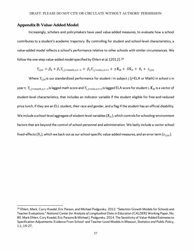
DRAFT: PLEASE DO NOT CITE OR CIRCULATE WITHOUT AUTHORS’ PERMISSION
57
Appendix B: Value-Added Model
Increasingly, scholars and policymakers have used value-added measures, to evaluate how a school
contributes to a student’s academic trajectory. By controlling for student and school-level characteristics, a
value-added model reflects a school’s performance relative to other schools with similar circumstances. We
follow the one-step value-added model specified by Ehlert et al. (2012).28
𝑌𝑌𝑖𝑖𝑖𝑖𝑖𝑖𝑖𝑖 = 𝛽𝛽0 + 𝛽𝛽1𝑌𝑌𝑖𝑖,𝑖𝑖=𝑖𝑖𝑚𝑚𝑖𝑖ℎ,𝑖𝑖,𝑖𝑖−1 + 𝛽𝛽2𝑌𝑌𝑖𝑖,𝑖𝑖=𝑖𝑖𝑒𝑒𝑚𝑚,𝑖𝑖,𝑖𝑖=1 + 𝛾𝛾𝑿𝑿𝒊𝒊𝒊𝒊 + 𝛿𝛿𝑺𝑺𝑖𝑖𝑖𝑖 + 𝜃𝜃𝑖𝑖 + 𝜀𝜀𝑖𝑖𝑖𝑖𝑖𝑖𝑖𝑖
Where 𝑌𝑌𝑖𝑖𝑖𝑖𝑖𝑖𝑖𝑖is our standardized performance for student i in subject j (j=ELA or Math) in school s in
year t; 𝑌𝑌𝑖𝑖,𝑖𝑖=𝑖𝑖𝑚𝑚𝑖𝑖ℎ,𝑖𝑖,𝑖𝑖−1is lagged math score and 𝑌𝑌𝑖𝑖,𝑖𝑖=𝑖𝑖𝑒𝑒𝑚𝑚,𝑖𝑖,𝑖𝑖=1is lagged ELA score for student i, 𝑿𝑿𝒊𝒊𝒊𝒊 is a vector of
student-level characteristics, that includes an indicator variable if the student eligible for free-and-reduced
price lunch, if they are an ELL student, their race and gender, and a flag if the student has an official disability.
We include a school-level aggregate of student-level variables (𝑺𝑺𝑖𝑖𝑖𝑖), which controls for schooling-environment
factors that are beyond the control of school personnel and administration. We lastly include a vector school
fixed-effects (𝜃𝜃𝑖𝑖), which we back out as our school-specific value-added measures, and an error term (𝜀𝜀𝑖𝑖𝑖𝑖𝑖𝑖𝑖𝑖).
28 Ehlert, Mark, Corry Koedel, Eric Parson, and Michael Podgursky. 2012. “Selection Growth Models for Schools and Teacher Evaluations.” National Center for Analysis of Longitudinal Data in Education (CALDER) Working Paper, No. 80. Mark Ehlert, Cory Koedel, Eric Parsons & Michael J. Podgursky. 2014. The Sensitivity of Value-Added Estimates to Specification Adjustments: Evidence From School- and Teacher-Level Models in Missouri, Statistics and Public Policy, 1:1, 19-27,

DRAFT: PLEASE DO NOT CITE OR CIRCULATE WITHOUT AUTHORS’ PERMISSION
58
Figure 1A: Closures in New York City
Indicates School Closure

DRAFT: PLEASE DO NOT CITE OR CIRCULATE WITHOUT AUTHORS’ PERMISSION
59
Figure A2: Event Study Result for Key Eight-Grade Outcomes for Eight-Grade Phaseout Cohorts
School-Level Outcomes
School-Level ELA School-Level Math
School-Level Value Added School-Level Distance Traveled
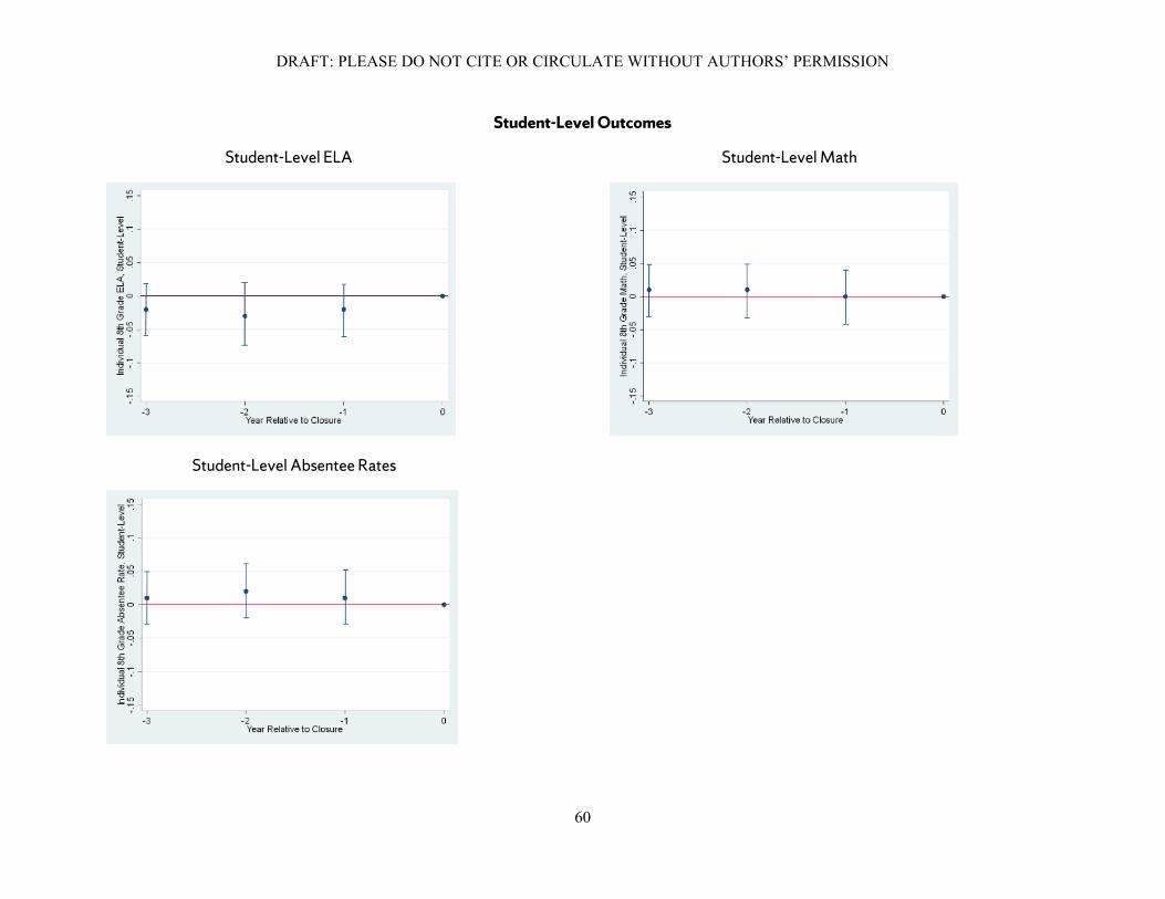
DRAFT: PLEASE DO NOT CITE OR CIRCULATE WITHOUT AUTHORS’ PERMISSION
60
Student-Level Outcomes
Student-Level ELA Student-Level Math
Student-Level Absentee Rates
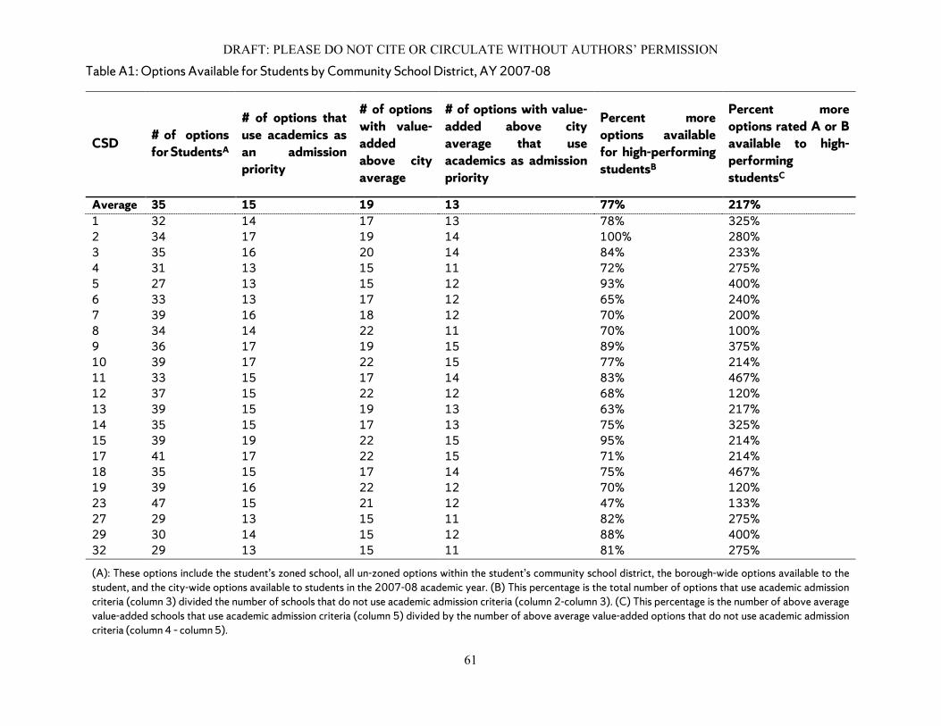
DRAFT: PLEASE DO NOT CITE OR CIRCULATE WITHOUT AUTHORS’ PERMISSION
61
Table A1: Options Available for Students by Community School District, AY 2007-08
CSD # of options for StudentsA
# of options that use academics as an admission priority
# of options with value-added above city average
# of options with value-added above city average that use academics as admission priority
Percent more options available for high-performing studentsB
Percent more options rated A or B available to high-performing studentsC
Average 35 15 19 13 77% 217% 1 32 14 17 13 78% 325% 2 34 17 19 14 100% 280% 3 35 16 20 14 84% 233% 4 31 13 15 11 72% 275% 5 27 13 15 12 93% 400% 6 33 13 17 12 65% 240% 7 39 16 18 12 70% 200% 8 34 14 22 11 70% 100% 9 36 17 19 15 89% 375% 10 39 17 22 15 77% 214% 11 33 15 17 14 83% 467% 12 37 15 22 12 68% 120% 13 39 15 19 13 63% 217% 14 35 15 17 13 75% 325% 15 39 19 22 15 95% 214% 17 41 17 22 15 71% 214% 18 35 15 17 14 75% 467% 19 39 16 22 12 70% 120% 23 47 15 21 12 47% 133% 27 29 13 15 11 82% 275% 29 30 14 15 12 88% 400% 32 29 13 15 11 81% 275%
(A): These options include the student’s zoned school, all un-zoned options within the student’s community school district, the borough-wide options available to the student, and the city-wide options available to students in the 2007-08 academic year. (B) This percentage is the total number of options that use academic admission criteria (column 3) divided the number of schools that do not use academic admission criteria (column 2-column 3). (C) This percentage is the number of above average value-added schools that use academic admission criteria (column 5) divided by the number of above average value-added options that do not use academic admission criteria (column 4 – column 5).

DRAFT: PLEASE DO NOT CITE OR CIRCULATE WITHOUT AUTHORS’ PERMISSION
62
Table A2: Effect of Closure and Phaseout on Seventh-Grade School Environment
(1) (2) (3) (4) (6) (7) (8) (9) (10)
Percent White
Percent Black
Percent Hispanic
Percent Asian
Percent FRPL Eligible
Distance to Schoolb
School Mathc School ELAc School Value
Addedd
Average Effect on Closure Cohort (CC)
0.035 -0.014 -0.010 0.022 -0.046 0.011 0.063* 0.060* 0.075* (0.020) (0.019) (0.019) (0.020) (0.029) (0.047) (0.035) (0.035) (0.042)
Average Effect on Phaseout Cohort (PC)
0.008 -0.010 -0.009 0.008 0.005 0.075 0.009 0.008 0.010 (0.020) (0.018) (0.018) (0.020) (0.029) (0.046) (0.035) (0.036) (0.043)
Effects by Quintile of Fifth-Grade Mathematics Scoree
Effect on CC Lowest Quintile -0.009 0.001 0.004 -0.002 -0.029 0.078 0.024 0.022 0.044 (0.030) (0.027) (0.027) (0.030) (0.035) (0.048) (0.037) (0.038) (0.046) Effect on CC in 20th – 40th Quintile 0.013 -0.006 -0.005 0.008 -0.034 0.084* 0.040 0.040 0.061 (0.029) (0.027) (0.027) (0.029) (0.035) (0.049) (0.037) (0.037) (0.045) Effect on CC in 40th – 60th Quintile 0.044 -0.013 -0.007 0.018 -0.049 0.101** 0.058 0.054 0.077* (0.030) (0.027) (0.027) (0.030) (0.035) (0.049) (0.038) (0.038) (0.045) Effect on CC in 60th – 80th Quintile 0.058** -0.020 -0.011 0.038 -0.048 0.131** 0.086** 0.084** 0.076* (0.029) (0.027) (0.027) (0.030) (0.035) (0.049) (0.038) (0.038) (0.046) Effect on CC in Top Quintile 0.069** -0.032 -0.031 0.044 -0.069 0.141*** 0.096** 0.090** 0.102** (0.030) (0.027) (0.027) (0.030) (0.035) (0.048) (0.038) (0.038) (0.046) Effect on PC in Bottom Quintile -0.004 0.005 -0.010 0.001 0.018 0.051 -0.020 -0.018 -0.016 (0.028) (0.024) (0.024) (0.027) (0.035) (0.048) (0.038) (0.038) (0.046) Effect on PC in 20th – 40th Quintile -0.003 -0.004 0.006 0.006 0.019 0.062 -0.006 -0.001 0.001 (0.027) (0.024) (0.024) (0.028) (0.035) (0.048) (0.037) (0.037) (0.046) Effect on PC in 40th – 60th Quintile 0.008 -0.008 0.004 0.004 0.011 0.068 0.018 0.014 0.015 (0.028) (0.024) (0.024) (0.028) (0.035) (0.048) (0.037) (0.038) (0.046) Effect on PC in 60th – 80th Quintile 0.014 -0.018 0.010 0.010 -0.004 0.091* 0.024 0.017 0.021 (0.028) (0.024) (0.023) (0.027) (0.035) (0.049) (0.038) (0.038) (0.046) Effect on PC in Top Quintile 0.025 -0.024 0.019 0.019 -0.019 0.101** 0.031 0.029 0.034 (0.027) (0.024) (0.024) (0.027) (0.035) (0.049) (0.037) (0.038) (0.046)
Notes: Number of Obs: 40,174. Standard errors robust to clustering by school are in parentheses, ***p<0.01, **p<0.05, *p<0.10. Student covariates, quadratics of student performance, and cohort fixed effects and elementary school fixed effects are included. (a) Percent from previous grade are the percent of students from each students fifth-grade school that also attend the same school with the student in sixth-grade. (b) Distance to School is the Euclidean distance (in miles) between the centroid of a student's assigned zip code and the school building. (c) ELA and Math are the lagged (prior-grade) performance for each student’s peers in seventh grade normalized at the year-grade-level for the schools in our sample. (d) Value-added measure captures the school’s contribution to a student’s test scores controlling for differences across schools and a student’s prior test scores. See Appendix A for a discussion of the value-added model used in this paper. (e) Estimates presented reflect the linear combination of the treatment indicator and each quintile interaction term.

DRAFT: PLEASE DO NOT CITE OR CIRCULATE WITHOUT AUTHORS’ PERMISSION
63
Table A3: Re-estimating Middle School Outcomes with the 130 Students with the Highest Probability of Attending a Closed School
(1) (2) (3) (4) (5) (6)
Avg. 6th Grade Math
Avg. 7th
Grade Math Avg. 8th Grade Math
Avg. 6th Grade ELA
Avg. 7th Grade ELA
Avg. 8th Grade ELA
Average Effect on Closure Cohort (CC) 0.028 0.019 0.017 0.024 0.015 0.021 (0.032) (0.032) (0.032) (0.032) (0.032) (0.032) Average Effect on Phaseout Cohort (PC) -0.011 -0.037 -0.058* -0.013 -0.027 -0.036 (0.032) (0.032) (0.033) (0.029) (0.030) (0.030) Effects by Fifth-Grade Mathematics Performance Effect on CC Lowest Quintile -0.024 -0.023 -0.036 -0.015 -0.013 -0.011 (0.036) (0.036) (0.037) (0.035) (0.035) (0.036) Effect on CC in 20th – 40th Quintile -0.011 -0.012 -0.004 -0.002 -0.005 0.002 (0.036) (0.036) (0.037) (0.035) (0.036) (0.036) Effect on CC in 40th – 60th Quintile 0.009 0.005 0.011 0.019 0.022 0.018 (0.036) (0.037) (0.037) (0.035) (0.035) (0.035) Effect on CC in 60th – 80th Quintile 0.051 0.048 0.056 0.055 0.048 0.045 (0.036) (0.036) (0.037) (0.035) (0.036) (0.036) Effect on CC in Top Quintile 0.072** 0.070** 0.062* 0.063* 0.062* 0.060* (0.036) (0.037) (0.037) (0.036) (0.036) (0.036) Effect on PC in Bottom Quintile -0.026 -0.053 -0.071** -0.028 -0.048 -0.066* (0.034) (0.034) (0.034) (0.035) (0.035) (0.035) Effect on PC in 20th – 40th Quintile -0.021 -0.044 -0.068* -0.021 -0.038 -0.058 (0.033) (0.034) (0.035) (0.035) (0.036) (0.036) Effect on PC in 40th – 60th Quintile -0.011 -0.038 -0.055 -0.011 -0.034 -0.051 (0.034) (0.034) (0.035) (0.035) (0.035) (0.036) Effect on PC in 60th – 80th Quintile 0.011 0.009 -0.028 -0.003 -0.011 -0.014 (0.033) (0.034) (0.034) (0.035) (0.035) (0.036) Effect on PC in Top Quintile 0.002 0.007 0.009 0.003 0.005 0.012 (0.033) (0.034) (0.035) (0.035) (0.036) (0.036) Obs 40,708 40,659 40,644 40,708 40,659 40,644
Notes: Standard errors robust to clustering by school are in parentheses, ***p<0.01, **p<0.05, *p<0.10.

DRAFT: PLEASE DO NOT CITE OR CIRCULATE WITHOUT AUTHORS’ PERMISSION
64
Table A4: Event Study Table when estimating the Model for Predicted Future Closure Cohorts
(1) (2) (3) (4) (5) (6) (7) (8) (9) Avg. 6th
Grade Math
Avg. 7th
Grade Math
Avg. 8th Grade Math
Avg. 6th Grade ELAa
Avg. 7th
Grade ELAa Avg. 8th Grade ELAa
6th Grade Absentee Rates
7th Grade Absentee Rates
8th Grade Absentee Rates
Closure (Lowest Quintile) in T-3 0.006 -0.009 -0.007 0.003 0.002 0.004 0.002 0.001 0.001 (0.047) (0.047) (0.048) (0.047) (0.047) (0.047) (0.039) (0.040) (0.040) Closure (Lowest Quintile) in T-2 0.002 -0.005 0.004 0.009 0.004 -0.006 -0.004 -0.006 -0.005 (0.047) (0.047) (0.047) (0.046) (0.046) (0.047) (0.039) (0.040) (0.040) Closure (Lowest Quintile) in T-1 -0.009 -0.010 -0.014 -0.008 0.000 -0.001 -0.006 0.003 -0.004 (0.047) (0.047) (0.048) (0.046) (0.046) (0.047) (0.039) (0.041) (0.040) Closure (Lowest Quintile) in T -0.022 -0.025 -0.026 -0.020 -0.019 -0.019 0.037 0.033 0.033 (0.047) (0.048) (0.048) (0.047) (0.047) (0.047) (0.039) (0.040) (0.040) Closure (Lowest Quintile) in T+1 -0.025 -0.030 -0.031 -0.024 -0.021 -0.021 0.038 0.035 0.033 (0.047) (0.047) (0.048) (0.046) (0.047) (0.047) (0.040) (0.040) (0.040) Closure (Lowest Quintile) in T+2 -0.014 -0.012 -0.019 -0.016 -0.013 -0.011 0.031 0.024 0.025 (0.047) (0.048) (0.048) (0.046) (0.047) (0.047) (0.039) (0.040) (0.040) Closure (20th – 40th) in T-3 -0.000 -0.005 -0.000 0.003 0.000 -0.004 0.005 0.002 0.004 (0.047) (0.047) (0.047) (0.046) (0.046) (0.047) (0.039) (0.040) (0.040) Closure (20th – 40th) in T-2 0.008 -0.008 -0.001 -0.003 -0.004 -0.004 0.005 -0.001 0.004 (0.047) (0.047) (0.047) (0.047) (0.047) (0.047) (0.039) (0.040) (0.040) Closure (20th – 40th) in T-1 0.012 -0.008 -0.000 0.004 -0.001 -0.004 0.002 0.002 0.000 (0.047) (0.047) (0.048) (0.047) (0.047) (0.047) (0.040) (0.040) (0.040) Closure (20th – 40th) in T -0.008 -0.007 -0.008 -0.007 -0.008 -0.010 0.021 0.028 0.024 (0.047) (0.047) (0.048) (0.047) (0.047) (0.047) (0.041) (0.041) (0.040) Closure (20th – 40th) in T+1 -0.004 -0.008 -0.007 -0.008 -0.008 -0.007 0.020 0.022 0.018 (0.047) (0.047) (0.047) (0.047) (0.047) (0.047) (0.040) (0.040) (0.040) Closure (20th – 40th) in T+2 0.000 -0.004 -0.008 -0.008 -0.009 0.000 0.020 0.022 0.020 (0.047) (0.047) (0.048) (0.046) (0.046) (0.047) (0.040) (0.040) (0.040) Closure (40th – 60th) in T-3 0.001 -0.002 0.002 0.001 0.000 -0.002 -0.001 0.001 -0.008 (0.047) (0.047) (0.048) (0.046) (0.046) (0.047) (0.040) (0.040) (0.040) Closure (40th – 60th) in T-2 0.005 0.004 -0.001 0.004 0.002 0.005 0.000 -0.002 0.001 (0.047) (0.047) (0.048) (0.046) (0.046) (0.047) (0.040) (0.040) (0.040)
Closure (40th – 60th) in T-1 0.005 0.005 -0.001 -0.002 -0.001 0.008 -0.002 0.001 -0.001 (0.047) (0.047) (0.048) (0.046) (0.046) (0.047) (0.040) (0.041) (0.040) Closure (40th – 60th) in T 0.009 0.011 0.011 0.008 0.009 0.010 0.021 0.020 0.018 (0.047) (0.047) (0.048) (0.046) (0.047) (0.047) (0.040) (0.040) (0.040) Closure (40th – 60th) in T+1 0.011 0.013 0.012 0.011 0.008 0.007 0.022 0.016 0.019 (0.047) (0.047) (0.048) (0.047) (0.047) (0.047) (0.039) (0.040) (0.040)

DRAFT: PLEASE DO NOT CITE OR CIRCULATE WITHOUT AUTHORS’ PERMISSION
65
(1) (2) (3) (4) (5) (6) (7) (8) (9) Avg. 6th
Grade Math
Avg. 7th
Grade Math
Avg. 8th Grade Math
Avg. 6th Grade ELAa
Avg. 7th
Grade ELAa Avg. 8th Grade ELAa
6th Grade Absentee Rates
7th Grade Absentee Rates
8th Grade Absentee Rates
Closure (40th – 60th) in T+2 0.008 0.011 0.011 0.009 0.011 0.007 0.011 0.010 0.010 (0.047) (0.047) (0.048) (0.047) (0.047) (0.048) (0.041) (0.040) (0.041) Closure (60th – 80th) in T-3 -0.004 -0.005 0.006 0.004 0.004 0.002 0.004 -0.001 0.002 (0.047) (0.047) (0.047) (0.047) (0.047) (0.047) (0.041) (0.040) (0.040) Closure (60th – 80th) in T-2 0.005 0.003 -0.003 -0.004 0.004 -0.003 0.004 -0.004 -0.002 (0.047) (0.047) (0.047) (0.046) (0.047) (0.047) (0.040) (0.040) (0.040) Closure (60th – 80th) in T-1 0.004 -0.006 -0.004 0.000 0.005 -0.004 0.003 -0.004 -0.001 (0.047) (0.047) (0.048) (0.046) (0.047) (0.047) (0.040) (0.040) (0.040) Closure (60th – 80th) in T 0.064 0.060 0.062 0.044 0.044 0.040 -0.008 -0.010 -0.008 (0.047) (0.047) (0.048) (0.047) (0.047) (0.047) (0.040) (0.040) (0.040) Closure (60th – 80th) in T+1 0.058 0.061 0.059 0.040 0.044 0.041 -0.011 -0.011 -0.004 (0.047) (0.047) (0.048) (0.047) (0.047) (0.047) (0.040) (0.040) (0.040) Closure (60th – 80th) in T+2 0.055 0.053 0.041 0.035 0.038 0.036 -0.008 -0.008 -0.004 (0.047) (0.047) (0.048) (0.046) (0.047) (0.047) (0.040) (0.040) (0.040) Closure (Top Quintile) in T-3 0.002 -0.002 0.008 -0.003 -0.005 0.004 -0.002 -0.005 -0.001 (0.047) (0.047) (0.048) (0.046) (0.047) (0.047) (0.040) (0.040) (0.040) Closure (Top Quintile) in T-2 -0.002 -0.003 0.004 -0.003 -0.004 0.000 0.002 0.000 0.001 (0.047) (0.047) (0.048) (0.046) (0.046) (0.047) (0.040) (0.040) (0.040) Closure (Top Quintile) in T-1 0.006 0.009 0.005 0.005 0.006 0.005 -0.002 0.001 0.001 (0.047) (0.047) (0.048) (0.046) (0.046) (0.047) (0.040) (0.040) (0.040) Closure (Top Quintile) in T 0.083* 0.082* 0.083* 0.071 0.066 0.067 -0.012 -0.010 -0.011 (0.047) (0.047) (0.047) (0.047) (0.047) (0.047) (0.040) (0.040) (0.041) Closure (Top Quintile) in T+1 0.079* 0.083* 0.080* 0.068 0.068 0.068 -0.010 -0.008 -0.008 (0.047) (0.047) (0.048) (0.047) (0.047) (0.047) (0.040) (0.040) (0.040) Closure (Top Quintile) in T+2 0.081* 0.082 0.078 0.070 0.070 0.068 -0.011 -0.008 -0.005 (0.047) (0.047) (0.047) (0.046) (0.046) (0.047) (0.040) (0.040) (0.041)
Notes: Number of Obs: 61,087 for sixth-grade outcomes, 60,985 for seventh-grade outcomes, and 60,703 for eighth-grade outcomes. Clustered by School Robust Standard Errors in Parentheses, ***p<0.01, **p<0.05, *p<0.10. Student Covariates, Quadratic of Lagged Test Scores, Cohort Fixed Effects and Elementary School Fixed Effects are included. Columns (1) through (3), and (7) through nine reflect fifth-grade Math performance distribution. Note (a): Columns (4) through (6) reflects fifth-grade ELA performance distribution. Phaseout indicator is included.

DRAFT: PLEASE DO NOT CITE OR CIRCULATE WITHOUT AUTHORS’ PERMISSION
66
Table A5: Estimated Effect of Switching to a Predicted-Cohort on Grade 6 School-Level Outcomes
(1) (2) (3) (4) (5) (6) (7) (8) (9) (10)
Percent White
Percent Black
Percent Hispanic
Percent Asian
Percent FRPL Eligible
Percent from Previous Grade
Distance Traveled School
Average Math Score
Average ELA Score
Average Value Added
Average Effect of Closure
0.013 -0.012 -0.010 0.010 -0.010 0.009 0.042 0.016 0.012 0.018
(0.018) (0.017) (0.017) (0.018) (0.027) (0.013) (0.045) (0.035) (0.034) (0.040) Effects by Fifth-Grade Mathematics Performance Effect on CC Lowest Quintile
-0.002 -0.006 -0.007 0.003 -0.012 0.002 0.034 0.015 0.004 0.014
(0.023) (0.021) (0.021) (0.025) (0.032) (0.018) (0.048) (0.039) (0.038) (0.044) Effect on CC in 20th – 40th Quintile
0.005 -0.010 -0.008 0.007 -0.011 0.005 0.044 0.016 0.011 0.011
(0.023) (0.021) (0.022) (0.025) (0.031) (0.019) (0.048) (0.039) (0.038) (0.044) Effect on CC in 40th – 60th Quintile
0.010 -0.007 -0.010 0.009 -0.010 0.011 0.044 0.015 0.014 0.021
(0.023) (0.022) (0.022) (0.025) (0.032) (0.019) (0.049) (0.039) (0.038) (0.044) Effect on CC in 60th – 80th Quintile
0.012 -0.009 -0.010 0.011 -0.010 0.016 0.047 0.018 0.014 0.020
(0.024) (0.021) (0.022) (0.024) (0.031) (0.019) (0.049) (0.039) (0.038) (0.044) Effect on CC in Top Quintile
0.014 -0.011 -0.009 0.012 -0.009 0.016 0.049 0.018 0.011 0.021
(0.023) (0.022) (0.023) (0.024) (0.031) (0.019) (0.049) (0.039) (0.038) (0.044)
Notes: Number of Obs: 40,227. Standard errors robust to clustering by school are in parentheses, ***p<0.01, **p<0.05, *p<0.10. Student covariates, quadratic lagged student performance, cohort fixed effects and elementary school fixed effects are included. See Table 5 for a description of outcome variables.

DRAFT: PLEASE DO NOT CITE OR CIRCULATE WITHOUT AUTHORS’ PERMISSION
67
Table A6: Estimate Effect of Switching to a Predicted-Cohort on Student-Level Outcomes
(1) (2) (3) Sixth-Grade Student-Level Math
Sixth-Grade Student-Level ELA
Sixth-Grade Student-Level Absentee Rates
Average effect on Closure Cohort (CC) 0.014 0.012 -0.004 (0.033) (0.031) (0.017) Effects by Fifth-Grade Mathematics Performance Effect on CC Lowest Quintile 0.009 0.006 -0.006 (0.038) (0.037) (0.025) Effect on CC in 20th – 40th Quintile 0.014 0.009 -0.006 (0.038) (0.037) (0.026) Effect on CC in 40th – 60th Quintile 0.013 0.011 -0.004 (0.038) (0.037) (0.025) Effect on CC in 60th – 80th Quintile 0.017 0.016 -0.002 (0.039) (0.037) (0.025) Effect on CC in Top Quintile 0.017 0.018 -0.003 (0.038) (0.037) (0.025)
Notes: Number of Obs: 39,602. Standard errors robust to clustering by school are in parentheses, ***p<0.01, **p<0.05, *p<0.10. Student covariates, quadratic of lagged student outcomes, cohort fixed effects and elementary school fixed effects are included. See Table 7 for a description of the outcome measures. For columns 1 and 3, these quintile brackets are based on pre-closure mathematics performance. For column 2 the within quintile effects of closure on closure and phaseout students is based on the pre-closure distribution of ELA test scores.