Whittlesey Creek 516(e) Sediment Impact Analysis Methods (SIAM)

Modeling Report

November, 2010 ________________________________________________

Prepared By: Great Lakes Hydraulics and Hydrology Office

________________________________________________

1

TABLE OF CONTENTS EXECUTIVE SUMMARY .......................................................................................... 2 

1.0   INTRODUCTION ........................................................................................... 3 1.1   Program Background ............................................................................................ 3 1.2   Watershed Information ......................................................................................... 3 

2.0   SITE INVESTIGATION .............................................................................. 8 

3.0   DATA AND HYDRAULIC MODEL DESCRIPTION ........................ 15 3.1   Flows .................................................................................................................. 15 3.2   Geometry Data ................................................................................................... 20 3.3   Software ............................................................................................................. 21 3.4  Modeling ............................................................................................................ 21 

4.0   SIAM BASELINE MODEL ....................................................................... 26 4.1   SIAM Purpose and Background ......................................................................... 26 4.2   SIAM Model Framework ................................................................................... 27 4.3  SIAM Input Data ................................................................................................ 31 

4.3.1  Bed Material Gradation ............................................................................... 31 4.3.2  Hydrology ................................................................................................... 32 4.3.3  Sediment Properties .................................................................................... 35 4.3.4  Sediment Sources ........................................................................................ 36 4.3.5  Hydraulics ................................................................................................... 38 

4.4  Whittlesey SIAM Baseline Model Output ......................................................... 39 4.5  SIAM Model Limitations ................................................................................... 43 

5.0   SIAM TUTORIAL AND SIAM MODEL ALTERNATIVES ........... 44 5.1  Getting Started with SIAM ................................................................................ 45 5.2  Large Woody Debris Restoration ....................................................................... 51 5.3  Floodplain Reconnection in LW5 ...................................................................... 56 5.4  Reduced Peak Flows .......................................................................................... 60 5.5  Bank Stabilization .............................................................................................. 63 5.6  Additional Restoration Scenarios and Model Limitations ................................. 70 

6.0   SUMMARY AND CONCLUSIONS ....................................................... 71 

REFERENCES ............................................................................................................. 73  APPENDIX A – BED GRADATIONS APPENDIX B – SIAM MODEL (ENCLOSED CD)

2

EXECUTIVE SUMMARY The US Army Corps of Engineers partnered with the US Fish and Wildlife Service, the US Geological Survey, and other local stakeholders to develop a Sediment Impact Analysis Methods (SIAM) model for the Whittlesey Creek watershed in Bayfield County, Wisconsin. Whittlesey Creek is considered a regionally important stream for fish spawning. The Whittlesey Creek National Wildlife Refuge was established to protect and restore habitat in Whittlesey Creek and the surrounding streams for migration, spawning and rearing of trout and salmon from Lake Superior. Long term goals of the National Wildlife Refuge include various restoration options; however, the interaction between some of the potential restoration options and the impacts to sedimentation and erosion is not fully understood. The Whittlesey Creek SIAM model was developed to screen these restoration scenarios and determine potential impacts to the sediment balance associated with various restoration and mitigation plans. A HEC-RAS steady state model was built to calculate the hydraulics of the system, an important component that SIAM requires to perform the sediment impact analysis. The USGS and Inter-Fluve, Inc. have collected significant amounts of sediment data including bed gradations, bank erosion rates, sediment loadings and gradations associated with overland flow, and sediment loadings from tributary inflows. Combined with the HEC-RAS steady state data, this sediment data was used in the SIAM model to construct a baseline case that was calibrated to known deposition and erosion rates in the Whittlesey Creek watershed. A total of four restoration scenarios have been modeled using SIAM. These include the addition of large woody debris, reduction in peak flows in the upper reaches, floodplain reconnection in the lower reaches, and bank stabilization in the mid-upper reaches. It was found that restorations that affected the hydraulics had the most significant effect on the sedimentation and erosion dynamics of the system. Also, SIAM found examples of potential unintended consequences of restoration to the sediment regime of downstream reaches. The SIAM model may be used to analyze additional restoration plans that local stakeholders may be considering. Most restoration scenarios have multiple objectives, and the effects of sediment are often not the driving reason behind restoration efforts. However, the interrelated impacts to sediment, hydraulics, and river morphology should be considered in all restoration designs. The analysis provided by SIAM for Whittlesey Creek can both determine the interrelated impacts of combined restoration scenarios, and determine if a downstream restoration will be filled by upstream sediment moving through the system or eroded due to the changes in the hydraulics of the restored reach. This powerful tool will allow local stakeholders to focus restoration efforts and money to the most feasible projects that have the greatest chance for long-term restoration success.

3

1.0 INTRODUCTION 1.1 Program Background This study was undertaken by the Detroit District Great Lakes Hydraulics and Hydrology Office to examine sediment transport in Whittlesey Creek, located in Bayfield County, Wisconsin. This work is authorized under Section 516(e) of the Water Resources Development Act (WRDA) of 1996, as amended, which directs the United States Army Corps of Engineers (USACE) to develop sediment modeling tools to reduce sediment loadings to federal navigation channels, federal harbors, or Great Lakes Areas of Concern (AOCs). Sedimentation and erosion are issues facing the Whittlesey Creek Watershed and it is important to understand the sediment dynamics of the system in order to design Best Management Practices (BMPs) and restoration scenarios. 1.2 Watershed Information The Whittlesey Creek watershed in Bayfield County, WI, (Figure 1) contributes flow to Lake Superior near Ashland, Wisconsin. The major tributaries of the watershed flow through highly erodible red clay, sand and gravel. Consequently erosion issues such as bank failures, major headcuts, and valley incision are prevalent throughout the watershed. In addition, many reaches are experiencing significant sedimentation including reaches that have become plugged with sediment. The baseflow in these plugged reaches flow as groundwater under the channel bed. The Whittlesey Creek watershed consists of a mix of forest and agricultural landuses (Figure 2). There are no major urban landuses within the watershed, and the population density is consequently low, at approximately 15 people per square mile. The watershed has a plateau in the uppermost reaches, steep slopes in the middle reaches, and a relatively flat depositional zone in the lower reaches (Figure 3). Many channels are significantly incised in the upper reaches, and the stream and valley morphology has been influenced by historic logging activities that peaked in the early 20th century.

4

5

Figure 2 – Whittlesey Creek Landuse (from USGS, 2003)

6

7

Whittlesey Creek is considered a regionally important stream for fish spawning (Wisconsin Department of Natural Resources, 1996). The Whittlesey Creek National Wildlife Refuge located near the mouth of the river was established to protect and restore habitat in Whittlesey Creek and the surrounding streams for migration, spawning and rearing of trout and salmon from Lake Superior. Aquatic habitat in Whittlesey Creek (Figure 4) is possibly negatively impacted by sedimentation problems due to runoff (Lenz et al., 2003). Long term goals of the National Wildlife Refuge include various restoration options; however, the interaction between some of the potential restoration options and the impacts to sedimentation and erosion is not fully understood. To this end, a sediment balance model, which can be used to screen restoration scenarios and determine potential impacts to sediment balance was developed as part of this study. This model, the Sediment Impact Analysis Methods (SIAM) was developed to examine sedimentation and erosion under present conditions and provide the local stakeholders with a model for rapidly examining the effects on sedimentation from several restoration alternatives.

Figure 4 – Distribution of brook trout fingerlings in Bayfield streams, 2004

8

2.0 SITE INVESTIGATION Site investigations were conducted in March of 2007 and April 2008 to collect data to support the sediment modeling. The primary focus of these site investigations included the following tasks:

1. Collect cross sectional data at selected locations to support the development of the hydraulic model of Whittlesey Creek

2. Install scour chains in the plugged reach to determine if the sediment is mobilized during a spring runoff.

3. Record observations related to the sedimentation and erosion potential of various reaches within the watershed.

In April 2007 cross section data were collected and scour chains were installed at three locations. The first location was 80 feet downstream of Cherryville Road Bridge where 2 scour chains were installed in a point bar composed of sand. The second cross section and scour chain were located just upstream of Galligan’s Ford, and the third location was just downstream of Galligan’s Ford. The purpose of collecting the cross sectional data and installing the scour chains was to determine the stability of the river morphology at these sections. The cross sectional data measures changes to widths and depths, which provides information related to whether the cross section is trending towards a depositional or erosive section. The scour chains provide a depth of maximum scour or erosion in order to determine the mobility of the bed. Combined, these methods provide valuable insight as to whether a reach is in dynamic equilibrium or is unstable. The stream located just downstream of Cherryville Road Bridge is very sandy and appears to be incised (Figures 5 and 6). The cross section was first surveyed on March 15, 2007 and resurveyed on April 21, 2008. These cross sections were compared to determine cross sectional area changes over the course of approximately one year (Figure 7). Overall, the cross section maintained the majority of its shape, however, the cross section did incise slightly (approximately 6 inches in some locations).

9

Figure 5 – Cross Section 80 Feet Downstream of Cherryville Bridge (Looking Upstream)

Figure 6 – Cross Section 80 Feet Downstream of Cherryville Bridge

10

Figure 7 – Cross Section 80 Feet Downstream of Cherryville Bridge

Scour chains were also installed at this location in 2007 and were re-visited in 2008. Two sets of chains were installed; one located at horizontal station 46.7 and one at 57.6. On April 21, 2008 both scour chains were located with a metal detector; however, on the one at station 46.7 could be recovered and measured. The chain at Station 57.6 feet set off the metal detector but due to the depth of the water, could not be recovered safely. It was estimated in the field that the chain was at least 6 inches under the sand; therefore, at least 6 inches of the chain depth was eroded. Since the bed in 2008 was approximately 3 inches lower than in 2007, the chain must have eroded at least 9 inches. The scour chain at 46.7 feet was recovered. When it was found, the chain anchor was found under six inches of sand on the bed of the channel (normally the anchor is at the deepest part of the channel), and the chain was tangled with roots. The chain and anchor were found at the same stationing as when it was installed, which shows that the sand bed eroded around it to a depth equal to the chain (approximately 1.8 feet). Both examples of the scour chains show that the sandy bed is very mobile, which is expected given the predominant grain size of the bed.

‐9

‐8

‐7

‐6

‐5

‐4

‐3

‐2

‐1

0

0 10 20 30 40 50 60 70 80 90 100

Elevation, ft

Station, ft

2007 2008

Scour chains installed at 46.7 and 57.6 station

11

The cross sections upstream and downstream of Galligan’s Ford were also surveyed in March 2007 and April 2008. This reach of river is plugged with sand, gravel, and cobble and, under baseflow conditions, no water is visible over the river. A runoff event was occurring during the data collection in 2007 (Figure 8). The cross sections collected in 2007 had coarser resolution (rounded to the nearest tenth of a foot) than the cross sectional data collected in 2008 (rounded to the nearest hundredth of a foot). The upstream cross section shows some deposition throughout the cross section (Figure 9) and the downstream cross section shows some erosion throughout the cross section (Figure 10). These two cross sections show no net deposition or erosion when the volume of sediment change is averaged between both cross sections.

Figure 8 – River Conditions Downstream of Galligan’s Ford

12

Figure 9 – Cross Section Upstream of Galligan’s Ford

Figure 10 – Cross Section Downstream of Galligan’s Ford

‐4.5

‐4

‐3.5

‐3

‐2.5

‐2

‐1.5

‐1

‐0.5

0

0 10 20 30 40 50 60

Elevation, ft

Station, ft

2007 2008

‐6

‐5

‐4

‐3

‐2

‐1

0

0 5 10 15 20 25 30 35 40 45

Elevation, ft

Station, ft

2007 2008

Scour chain installed at 27.0

station

Scour chain installed at 21.0

station

13

Scour chains were also installed both upstream and downstream of Galligan’s Ford in 2007. Due to the ice conditions, only 6 inches (approximately) of chain were installed at the upstream locations and 18 inches at the downstream location due to the frozen bed. A runoff event occurred during the scour chain installation in 2007 (Figure 11). During this event it was observed that the runoff water flowed over the sediment and did not entrain most of the smaller particles because the particles were frozen with each other and with the bed. This frozen sediment conglomerate protected the sediment plug from migrating downstream during this event. It is uncertain as to whether the frozen conditions are typical of spring runoff. However, the scour chains were found in the same location without any erosion or bed movement in 2008.

Figure 11 – Installation of Scour Chains near Galligan’s Ford, March 2007

During a site visit in May, 2010 the downstream scour chain was found approximately 20 yards downstream of the installation location and was fully exposed (Figure 12). This shows that although during 2007 and 2008 the bed was not mobile, from 2008 to 2010

14

the bed sediment did transport downstream. Due to the transport of the heavy chain, it is assumed that the cobbles (as well as gravel and sand) are moving downstream through this plugged reach. The movement of this sediment (particularly the sand) should be accounted for in restoration planning.

Figure 12 – Location of Scour Chain near Galligan’s Ford, May 2010

15

3.0 DATA AND HYDRAULIC MODEL DESCRIPTION In order to develop a Sediment Impact Analysis Methods (SIAM) model, a steady state hydraulic model of the watershed was first developed and used to calculate hydraulic variables required by SIAM. The following sections describe the development of the steady state hydraulic model of the Whittlesey Creek watershed including the North Fork Creek, Whittlesey Upper, and Whittlesey Lower streams.

3.1 Flows

When sediment transport modeling is conducted, a storm flow between 1.5 and 2 years is often used as a surrogate for the wide range of flows that a river experiences. This recurrence interval is approximately equal to the effective discharge of a stream and generally is accepted as the flow that significantly influences the channel dimensions. Due to the importance of this flow the steady state hydraulic model for the Whittlesey Creek was developed using the 1.5 year return interval. The computer software HEC-SSP and the USGS gage in the downstream region of Whittlesey Creek (Gage 040263205 near Ashland, WI) were used to determine this flowrate at the mouth of the river. This flowrate was then scaled using standard practices described in this report to determine the effective discharge at various locations throughout the watershed. The USGS Gage 040263205 includes eleven annual peak flow events dating back from 1999 (the first year of record for the gage) through 2009. These peak flows were used in the flood frequency statistical analysis to determine the 1.5 year recurrence interval (66.7% chance exceedance event). These flow events are shown in Table 1.

Table 1 – Annual Peak Flows for USGS Gage 040263205

Date of Event

Flow (cfs)

5-Jul-99 710 29-Feb-00 60 23-Apr-01 777 11-Apr-02 580 11-May-03 432 19-Apr-04 319 30-Jun-05 230 5-Oct-06 851

13-Mar-07 174 3-May-08 418 16-Mar-09 111

16

The peak flows were input into HEC-SSP and an exceedance probability curve was generated for the data, assuming a Weibull distribution. There were no statistical outliers outside of the 95% confidence interval for this dataset. Moreover, the expected probability curve closely matches the computed curve using the Weibull distribution. The resulting bankfull flow (assumed as the 1.5-year flow for this analysis) was calculated as 232 cfs using this method (Figure 13 and Table 2).

In order to determine the outflows for the Upper Whittlesey and North Fork, the USGS regression equations were adopted from the USGS report 03-4250: Flood-Frequency Characteristics of Wisconsin Streams (Walter & Krug, 2003). For the sub-basins of the Upper Whittlesey and North Fork, drainage areas and channel slopes were determined using Table 3 from the USGS Report 03-4130: Simulation of Ground-Water Flow and Rainfall Runoff with Emphasis on the Effects of Land Cover, Whittlesey Creek, Bayfield County, Wisconsin, 1999-2001 (Lenz et al., 2003). This report used the Soil and Water Assessment Tool (SWAT) to examine groundwater flow, rainfall and runoff and is available at the following URL:

http://pubs.usgs.gov/wri/wrir-03-4130/pdf/wrir03-4130.pdf Table 3 lists all of the input variables for each subwatershed listed in the USGS Report 03-4130.

17

Figure 13

18

Table 2 – HEC-SSP Computed Flows for USGS Gage 040263205 Percent Chance

Exceedance

Computed Curve Flow,

cfs

Expected Prob. Flow, cfs

0.05 Confidence

Limit Flow, cfs

0.95 Confidence

Limit Flow, cfs0.1 3183.2 6522.8 13303.8 1556.2 1.0 1960.6 2809.3 6330.1 1066.3 5.0 1225.5 1459.8 3118.7 730.0 10.0 939.9 1050.0 2109.6 584.1 50.0 338.3 338.3 537.3 215.9 66.7 232.4 225.7 355.4 136.9 99.0 37.0 20.2 73.8 9.4

Table 3 – Input Variables for Whittlesey Subwatershed Flow Calculations

Basin Watercourse Area,

sq. miles

ST Length,

mi

Weighted Slope, ft/mile

SP Snowfall, in/year

1 Whittelsey Upper 1.12 1 1.304 79.2 2.19 71.5 2 Whittelsey Upper 0.49 1 0.19 93.66261 2.19 71.5 3 Whittelsey Upper 0.108 1 0.5 93.41728 2.19 71.5 15 Whittelsey Upper 0.772 1 0.87 111.9275 2.19 71.5 16 Whittelsey Upper 0.587 1 1.5 163.68 2.19 71.5 5 Whittelsey Upper 0.281 1 0.62 116.91 2.19 71.5 6 Whittelsey Upper 0.278 1 0.56 112.8157 2.19 71.5 18 Whittelsey Upper 0.479 1 1.4 168.96 2.19 71.5 7 Whittelsey Upper 0.0618 1 0.24 118.3664 2.19 71.5

4 North Fork 1.64 1 2.5 89.76 2.19 71.5 17 North Fork 0.39 1 1.6 92.80315 2.19 71.5 8 North Fork 0.131 1 0.68 91.01831 2.19 71.5

19 Whittelsey Main 0.166 1 0.5 107.4713 2.19 71.5 9 Whittelsey Main 0.355 1 1.4 126.72 2.19 71.5 10 Whittelsey Main 0.127 1 0.31 107.1676 2.19 71.5 11 Whittelsey Main 0.0579 1 0.31 106.3734 2.19 71.5 12 Whittelsey Main 0.0541 1 0.43 105.7236 2.19 71.5 13 Whittelsey Main 0.0541 1 0.56 105.0837 2.19 71.5 14 Whittelsey Main 0.0309 1 0.25 104.6997 2.19 71.5

ST = Storage Ratio SP = Soil Permeability, in/hour See Figure 2 of this report for Basin Boundaries

19

The Sites on Streams near Streamflow-Gaging Station method described in the USGS Report 03-4250 was used to calculate the ungaged upper region flowrates. This method uses an adjustment ratio (r’), which includes both the flood flow values calculated from the gaging station and regression formulas calculated for regions of the State of Wisconsin. The calculated flowrates for the various basins of the Whittlesey Creek are found in Table 4. The final flowrates were converted to metric units to be included in the HEC-RAS model.

Table 4 – Flow Values Used in the HEC-RAS Model

Basin Watercourse ^

Qu, cfs r' Qu, cfs Upstream Reach, ft

HEC-RAS Input Q, cms

1 Whittelsey Upper 66.91 1.26 84.08 NA NA 2 Whittelsey Upper 95.94 1.21 115.67 11068 3.275 3 Whittelsey Upper 101.41 1.19 121.12 10637 3.430 15 Whittelsey Upper 146.97 1.11 163.77 9227 4.637 16 Whittelsey Upper 46.89 1.31 61.51 NA NA 5 Whittelsey Upper 192.63 1.02 197.29 6740 5.587 6 Whittelsey Upper 204.29 1.00 203.34 5848 5.758 18 Whittelsey Upper 39.68 1.32 52.50 NA NA 7 Whittelsey Upper 233.39 0.94 219.21 4768 6.207 4 North Fork 96.34 1.20 115.85 5008 3.280 17 North Fork 116.92 1.16 135.86 3673 3.847 8 North Fork 122.74 1.15 140.96 1119 3.992

14 Whittelsey Main 360.29 0.63 226.00 826 6.400 13 Whittelsey Main 359.32 0.63 226.54 1602 6.415 12 Whittelsey Main 357.57 0.64 227.45 2422 6.441 11 Whittelsey Main 355.83 0.64 228.34 3041 6.466 9 Whittelsey Main 28.27 1.34 37.77 NA NA 10 Whittelsey Main 354.03 0.65 229.31 3475 6.493 19 Whittelsey Main 333.09 0.70 232.41 4211 6.581

20

3.2 Geometry Data

Survey data of Whittlesey Creek was collected in 2006 and 2007. It included several cross-sections including some at 5 different bridges and 2 culverts. Because ground truth survey data was sparse for the Upper Whittlesey and North Fork, a 5-meter resolution Digital Elevation Model (DEM) was used to extract topographic and cross section data. The DEM was adjusted by adding additional detail such as channel widths and depths collected at some locations by the USGS. The interpolated TIN is shown in Figure 14 with the cross sections and survey data overlaid.

Figure 14 – Whittlesey Creek TIN and Model Cross Sections

21

3.3 Software

Hydraulic calculations were performed using the Hydraulic Engineering Center River Analysis System (HEC-RAS), version 4.1. HEC-RAS is comprised of a Graphical User Interface (GUI), separate hydraulic analysis components, data storage and management capabilities, graphics and reporting facilities. HEC-RAS is also the computational software used to compute the hydraulic inputs for the SIAM model. The HEC-RAS system contains four one-dimensional river analysis components for : (1) steady flow water surface profile computations; (2) unsteady flow simulations; (3) movable boundary sediment transport computations; and (4) water quality analysis. A key element is that all four components use a common geometric data representation and common geometric and hydraulic computation routines. In addition to the four river analysis components, the system contains several hydraulic design features that can be invoked once the basic water surface profiles are computed.

3.4 Modeling

One hundred and forty-two (142) cross sections were created using ArcGIS and HEC-GeoRAS. HEC-GeoRAS is a set of procedures, tools, and utilities for processing geospatial data in ArcGIS using a graphical user interface (GUI). The interface allows the preparation of geometric data for import into HEC-RAS and processes simulation results exported from HEC-RAS. The final geometry file is shown in Figure 15, and the profiles of each reach are shown in Figures 16, 17 and 18.

22

Figure 15 – Whittlesey Creek Geometry File in HEC-RAS

23

Figure 16 – North Fork Profile

Figure 17 - Upper Reach Profile

0 1 2 3 4 5200

220

240

260

280

300

320

WhittleseySIAM Plan: 1.5yr Steady State 10/20/2010

Main Channel Di stance (km)

Ele

vatio

n (m

)Legend

WS PF 1

Crit PF 1

Ground

North Fork North Fork

0 1 2 3 4 5 6 7200

220

240

260

280

300

320

WhittleseySIAM Plan: 1.5yr Steady State 10/20/2010

Main Channel Di stance (km)

Ele

vatio

n (m

)

Legend

WS PF 1

Crit PF 1

Ground

Whitt lesey Whittesey Upper

24

Figure 18 – Lower Whittlesey Profile

On September 10, 2008, the USGS surveyed the datum of the USGS gage located on the Lower Whittlesey Creek. The elevation was found to be 185.85 m. The purpose of gathering this elevation was to aid in calibrating the hydraulic model. In order to calibrate the model, a regression analysis was performed on the peak flow data shown in Table 1. The stage was then found for the 1.5-year design flow of 232 cfs (6.570 cms). Figure 19 shows the results:

0 1 2 3 4 5182

184

186

188

190

192

194

196

198

200

WhittleseySIAM Plan: 1.5yr Steady State 10/20/2010

Main Channel Di stance (km)

Ele

vatio

n (m

)

Legend

WS PF 1

Crit PF 1

Ground

Whitt lesey Whittlesey Lower

25

Figure 19 – USGS Rating Curve at Whittlesey Creek Gage 040263205

The trendline equation yielded a stage of 186.93 m for the 1.5-year flow. The location of the USGS gage is between Station 1691 and 1634. The calculated hydraulic profile elevations at these two stations are 187.20 m and 186.78 m respectively for the 1.5-year flow. The elevation of 186.93 at the USGS gage is between these two elevations, showing that stage in the model calibrates to the known elevation at the gage location.

y = -0.0016x2 + 0.1035x + 186.32R2 = 0.9969

186.20

186.40

186.60

186.80

187.00

187.20

187.40

187.60

187.80

0.00 5.00 10.00 15.00 20.00 25.00 30.00

Sta

ge

(m)

Q (cms)

Peak Flows

Poly. (Peak Flows)

26

4.0 SIAM BASELINE MODEL River restoration is most successful when accounting for system interactions with the proposed restoration design. Sedimentation or erosion effects can undermine, bury, or leave restoration efforts stranded. Traditional means of evaluating sediment impacts include sediment continuity analysis and mobile boundary hydraulic modeling. At the evaluation of alternatives stage of restoration, this type of detailed modeling is often cost prohibitive and rarely done for all alternatives. The Sediment Impact Analysis Methods (SIAM) provides a framework for combining morphological, hydrologic, and hydraulic information to assess sediment impacts associated with various restoration scenarios or hydrologic regimes at a level that is appropriate for evaluating and screening alternatives. The results of a SIAM model provide insight into impacts of sediment balance throughout the watershed, which is more detailed than a qualitative geomorphic evaluation and less intensive than a numeric mobile boundary model. SIAM represents a stream network as a series of homogeneous reaches and defines the connectivity between reaches. This approach creates a sediment linkage model for evaluating impacts of local changes from a sediment continuity perspective throughout the system being modeled. Potential short and long term imbalances and instabilities in a channel network can be mapped, and may be used to provide the first step in identifying problem areas and designing or refining remediation. The procedures allow for a rapid assessment of dynamic equilibrium in channel networks to target the source of problems and develop restoration recommendations.

4.1 SIAM Purpose and Background

The purpose of developing the SIAM model for Whittlesey Creek is to provide local stakeholders a model that can be used to examine various watershed management restoration scenarios and techniques to assess the feasibility of restoring coaster brook trout and other habitat. A key component of SIAM is its ability to track sediment transport potential through the system by grain size and to account for the spatial variations in the wash load/bed-material load thresholds. This allows SIAM to quantify the bed material-driven morphologic impacts and route the wash load through the system. SIAM is currently embedded in the Hydraulic Design (HD) Module of HEC-RAS 4.1. HEC-RAS 4.1 can be obtained from the Hydrologic Engineering Center website at the following URL:

http://www.hec.usace.army.mil.

27

Six sediment transport functions are available for SIAM computations. These include:

1. Ackers-White (1973) 2. Engelund – Hansen (1967) 3. Laursen (Copeland) (1968/1989) 4. Meyer-Peter Muller (1948) 5. Toffaleti (1968) 6. Yang (1973/1984)

SIAM can distinguish between wash load and bed-material load based on a user-defined threshold diameter. Bed-material local balance is computed as the difference between bed-material supply and sediment transport capacity, whereas the wash load is routed through the model. Computations are performed by grain size class on a reach average basis. The hydraulics necessary to perform the sediment transport calculations are provided directly from the shallow-water computations performed in HEC-RAS. SIAM empowers designers and planners to consider sediment supply and transport in management and rehabilitation of channel systems.

4.2 SIAM Model Framework

The calibrated steady state hydraulic HEC-RAS model was used to develop a base SIAM model that could easily be modified to examine proposed restoration alternatives in the Whittlesey watershed. The first step in SIAM is to subdivide the HEC-RAS hydraulic model into sediment reaches. A sediment reach is a grouping of cross sections with relatively consistent hydraulic and sediment properties. Sediment reaches are established using river cross section stationing from the existing HEC-RAS model geometry profile. Beginning and ending cross section stations for each reach must not overlap and are selected where there are significant changes in hydraulic properties, hydrology or sediment data. The reaches must begin at the next cross section downstream of the prior reach and should be selected at least two cross sections upstream or downstream of a bridge. Sediment reaches must be defined so that all cross sections are included within only one sediment reach. Sediment reaches cannot cross junctions and must exist entirely within the same hydraulic reach. Initially, ten SIAM sediment reaches were set up by river and reach (three on North Fork, three on Upper Whittlesey Creek, four on Lower Whittlesey Creek). For each River Reach, a Sediment Reach (Sed Reach) was given a name, an Upstream River Station (US RS) and Downstream River Station (DS RS). Initial Sediment reaches are listed in Table 5:

28

Table 5 – Initial SIAM Sediment Reaches

River Reach Sediment

Reach ID Downstream River Station

Upstream River Station

North Fork Creek

North Fork NF1 4106.696 5008.337 NF2 1524.88 3789.981 NF3 89.86793 1407.729

Whittlesey Creek

Upper Whittlesey

UW1 10447.36 11068 UW2 7141.820 10358.56 UW3 4357.443 6994.606

Whittlesey Creek

Lower Whittlesey

LW1 3474.567 4211.304 LW2 2535.207 3206.805 LW3 1602.723 2470.273 LW4 8.230177 1532.687

Consultation with Dr. Faith Fitzpatrick, USGS, resulted in modifying sediment reaches due to significant changes in bed gradation and sediment sources within some of the initial sediment reaches. Some sediment reaches were split into two reaches. The reaches were renumbered, and upstream and downstream river stationing changed as shown in Table 6:

Table 6 – Revised (Final) SIAM Sediment Reaches

River Reach Sediment

Reach ID Downstream River Station

Upstream River Station

North Fork Creek

North Fork NF1 4106.696 5008.337 NF2 1407.729 3789.981 NF3 89.86793 1118.989

Whittlesey Creek

Upper Whittlesey

UW1 10447.36 11068 UW2 8863.591 10358.56 UW3 7141.827 8633.682 UW4 6323.932 6994.606 UW5 5173.338 6156.891 UW6 4357.443 5067.517

Whittlesey Creek

Lower Whittlesey

LW1 3474.567 4211.304 LW2 2535.207 3206.805 LW3 1868.313 2470.273 LW4 1602.723 1826.96 LW5 874.364 1532.687 LW6 8.230177 826.1825

Figure 20 shows the boundaries of each delineated reach, and some of the features found in the watershed.

29

30

Once sediment reaches are defined, SIAM requires data for input into five categories of river variables. These include:

1. Bed Mat’l (Bed Material gradation data) 2. Hydro (Annualized flow duration) 3. Sed Prop (A variety of sediment properties required to run the model) 4. Sources (Local and annual Sediment Sources to the reach) 5. Hydraulics (Reach weighted averaged hydraulic parameters for the sediment

reach automatically populated by HEC-RAS). The following sections describe the data used for each variable in the SIAM Model.

31

4.3 SIAM Input Data

4.3.1 Bed Material Gradation

Each sediment reach was given a bed material sampling name by selecting the Create a Bed Sampling record icon in the Hydraulic Design file, typing in a filename and selecting OK. A significant amount of bed gradation data in the form of pebble counts and bag samples were collected by the USGS and Inter-Fluve, Inc. A sample bed gradation from USGS pebble counts for the first sediment reach on North Fork is identified as BedNF1pc (Table 7). Note the pebble count percent finer values of 7.37 for particle size diameters 0.5 mm, 1 mm, 2 mm and 4 mm were altered slightly in order for SIAM to track all particle sizes within the range of collected data.

Table 7 – USGS Pebble Count and SIAM Bed Gradation Data

North Fork SIAM Reach NF1 (BedNF1pc)

The sediment gradations for all bed samples collected by the USGS and Inter-Fluve, Inc. are provided in Appendix A of this report.

Particle Size Dia., mm

% Finer Pebble count data

% Finer used in SIAM

0.062 1.05 1.05 0.125 2.11 2.11 0.25 6.32 6.32 0.5 7.37 7.34 1 7.37 7.35 2 7.37 7.36 4 7.37 7.37 8 9.47 9.47 16 17.89 17.89 32 33.68 33.68 64 54.74 54.74 128 73.68 73.68 256 92.63 92.63 512 100 100

32

4.3.2 Hydrology

The second category of data that SIAM uses is the Hydrology data for the stream reaches. The profile column of the hydrology tab is automatically populated with the profiles associated with the steady flow file of the current plan. The Ch Q column is also automatically populated with a sediment reach length-weighted channel discharge that is extracted from the output of a steady state HEC-RAS simulation. SIAM predicts annual trends and is based on an annualized flow duration curve. Therefore, the populated discharges for the profiles must be assigned a duration period in days that is representative of the annual flow duration. The duration increments in the Duration column for each profile are in units of days per year. Temperature associated with the flow is also required and can be varied seasonally; however, for the Whittlesey Creek an average value of 13° Celsius was used since many of the flows occur numerous times throughout the year and because temperature will have a negligible effect on the transport of sand and other larger particles typical of the Whittlesey Creek. The flow duration data was determined using 15-minute data from the Ashland gage for a 10-year period between 1999 and 2009. A frequency analysis was performed on the data to determine durations applied in the SIAM model. Ten bins were selected to represent the range of flows extracted from the gage. Since the gage is located in the fourth reach of the Lower Whittlesey Creek (measured from upstream) the frequency analysis performed applies to the hydrology of the LW4 sediment reach. Output from this frequency analysis is shown in Table 8 for this location. This table shows that the majority of the flow record (approximately 90%) can be represented by a small range of flows (0.69 cms to 1.1 cms). Consequently, the flow duration curve used for the LW4 reach incorporates the midrange baseflow value of 0.90 cms, which occurs 332.5 days out of the year. The majority of the remaining flow occurs at higher flowrates with the largest flowrate of 38.5 cms occurring 0.06 days (86 minutes) out of the year.

33

Table 8 – Frequency Analysis of LW4 Reach for Water years 1999-2009

Qbin, cms

Frequency

Exceedance

Qmid

interval, cms

Annual Days Absolute Cumulative percent

0.43 1 1 2.93E-06 100% 0.56 0.1 0.69 310810 310811 0.919 8.90% 0.90 332.51 1.10 18951 329762 0.966 3.35% 1.43 20.27 1.76 6523 33.6285 0.986 1.44% 2.29 6.98 2.82 5607 338892 0.993 0.67% 3.67 2.79 4.52 1155 340047 0.997 0.33% 5.87 1.24 7.23 582 340629 0.998 0.16% 9.40 0.62 11.57 316 340945 0.999 0.07% 15.05 0.34 18.52 182 341127 0.9998 0.02% 24.08 0.19 29.64 56 341183 1 0.00% 38.54 0.06 47.43 0 341183 1 0.00% 47.43 0.00

The flow calculated at the gage is scaled based on the watershed drainage area of each reach. The ratio to gage area for each reach is shown in Table 9.

Table 9 – Scaling Factor for Flow-Duration Curve for each SIAM Reach

Reach

Area, square miles

Cummulative Area,

square miles Ratio to

gage North Fork1 1.64 1.64 0.231 North Fork2 0.39 2.03 0.286 North Fork3 0.13 2.16 0.304 Whittlesey Upper1 1.61 1.61 0.227 Whittlesey Upper2 0.11 1.72 0.242 Whittlesey Upper3 0.77 2.49 0.351 Whittlesey Upper4 0.87 3.36 0.473 Whittlesey Upper5 0.28 3.64 0.512 Whittlesey Upper6 0.54 4.18 0.588 Whittlesey Lower1 0.17 6.50 0.916 Whittlesey Lower2 0.48 6.98 0.984 Whittlesey Lower3 0.06 7.04 0.992 Whittlesey Lower4 0.05 7.10 1.000 Whittlesey Lower5 0.05 7.15 1.008 Whittlesey Lower6 0.03 7.18 1.012

34

The scaled flowrates based on the USGS flow duration analysis and scaling factor are shown in Table 10.

Table 10 – Flow rate data, in cms, for each Reach Using Scaling Factor

Duration, days → 0.1 333 20.3 6.98 2.79 1.24 0.62 0.34 0.19 0.1 Reach RS, m Qpf1 Qpf2 Qpf3 Qpf4 Qpf5 Qpf6 Qpf7 Qpf8 Qpf9 Qpf10

NF1 5008 0.13 0.21 0.33 0.53 0.85 1.36 2.17 3.48 5.56 8.90NF2 3672 0.16 0.26 0.41 0.65 1.05 1.68 2.69 4.30 6.89 11.02NF3 1119 0.17 0.27 0.43 0.70 1.12 1.78 2.86 4.58 7.32 11.72UW1 11068 0.13 0.20 0.32 0.52 0.83 1.33 2.13 3.42 5.47 8.75UW2 10637 0.14 0.22 0.35 0.55 0.89 1.42 2.27 3.64 5.83 9.33UW3 9227 0.20 0.32 0.50 0.80 1.29 2.06 3.30 5.28 8.45 13.53UW4 6740 0.26 0.43 0.68 1.08 1.74 2.78 4.45 7.12 11.39 18.23UW5 5848 0.29 0.46 0.73 1.17 1.88 3.01 4.81 7.71 12.33 19.73UW6 4768 0.33 0.53 0.84 1.35 2.16 3.45 5.53 8.85 14.16 22.66LW1 4211 0.51 0.82 1.31 2.10 3.36 5.38 8.61 13.79 22.06 35.30LW2 3475 0.55 0.89 1.41 2.25 3.61 5.78 9.25 14.81 23.69 37.92LW3 3041 0.56 0.89 1.42 2.27 3.64 5.82 9.32 14.93 23.89 38.23LW4 2422 0.56 0.90 1.43 2.29 3.67 5.87 9.40 15.05 24.08 38.54LW5 1603 0.56 0.91 1.44 2.31 3.70 5.92 9.48 15.17 24.27 38.85LW6 826 0.57 0.91 1.45 2.32 3.71 5.94 9.51 15.23 24.37 39.00

Only the flowrates are scaled based on drainage area, and therefore the durations associated with each bin of flow (pf 1-10) are the same for all reaches. In many of the reaches upstream of the junction of Upper Whittlesey and North Fork baseflow is not present in the main channel, but flows under the streambed. Therefore, the baseflow for each of the reaches upstream of LW1 were removed from the flow file and were input into a Steady State Flow file (existing_siam.f05). Table 11 displays the results of the hydrology calculated for each of the Whittlesey reaches.

35

Table 11 – Flow rate data, in cms, for each Reach in SIAM (Baseflow in Upper Reaches Removed)

Duration, days → 0.1 333 20.3 6.98 2.79 1.24 0.62 0.34 0.19 0.1

Reach RS, m Qpf1 Qpf2 Qpf3 Qpf4 Qpf5 Qpf6 Qpf7 Qpf8 Qpf9 Qpf10 NF1 5008 0.01 0.01 0.12 0.32 0.64 1.15 1.96 3.27 5.35 8.69 NF2 3672 0.01 0.01 0.15 0.39 0.79 1.42 2.43 4.04 6.63 10.76NF3 1119 0.01 0.01 0.16 0.43 0.85 1.51 2.59 4.31 7.05 11.45UW1 11068 0.01 0.01 0.12 0.32 0.63 1.13 1.93 3.22 5.27 8.55 UW2 10637 0.01 0.01 0.13 0.33 0.67 1.2 2.05 3.42 5.61 9.11 UW3 9227 0.01 0.01 0.18 0.48 0.97 1.74 2.98 4.96 8.13 13.21UW4 6740 0.01 0.01 0.25 0.65 1.31 2.35 4.02 6.69 10.96 17.8 UW5 5848 0.01 0.01 0.27 0.71 1.42 2.55 4.35 7.25 11.87 19.27UW6 4768 0.01 0.01 0.31 0.82 1.63 2.92 5 8.32 13.63 22.13LW1 4211 0.51 0.82 1.31 2.1 3.36 5.38 8.61 13.79 22.06 35.3 LW2 3475 0.55 0.89 1.41 2.25 3.61 5.78 9.25 14.81 23.69 37.92LW3 3041 0.56 0.89 1.42 2.27 3.64 5.82 9.32 14.93 23.89 38.23LW4 2422 0.56 0.9 1.43 2.29 3.67 5.87 9.4 15.05 24.08 38.54LW5 1603 0.56 0.91 1.44 2.31 3.7 5.92 9.48 15.17 24.27 38.85LW6 826 0.57 0.91 1.45 2.32 3.71 5.94 9.51 15.23 24.37 39

4.3.3 Sediment Properties

SIAM has six sediment transport functions available to compute the annualized transport capacity. The Meyer-Peter Müller sediment transport function is appropriate for coarse bed streams, and was therefore selected as the method to compute sediment capacity at most of the reaches. The only exceptions were the three lowest reaches (LW6, LW5, and LW4), which were modeled using the Laursen (Copeland) equation. This equation is more appropriate for the predominately sandy channel that exists in these lower reaches. The Fall Velocity method was set to Default, which uses the method associated with the respective transport function. Wash load is the material in the suspended sediment load, but not present in appreciable quantities in the bed. The Wash Load Max Class lists 10 grade classes and their upper bound particle size in mm. A wash load threshold of 0.25 mm was used in the SIAM model for most reaches, and corresponds to fine sands. This value was chosen based on the small percentage of fine sands in the majority of the sediment reaches. Exceptions to this value are located at the uppermost reaches of the system (NF1, NF2, UW1, and UW2). The wash load particle diameter was increased at these locations in order to calibrate the sediment balance at these upstream reaches. The Specific Gravity default of 2.65 was used in this model. The concentration of fine sediments is an optional value used to adjust the transport rate for high concentration scenarios. The adjustment is based on a correction factor that accounts for the effects of fine sediment and temperature on kinematic viscosity, and consequently particle fall velocity. This adjustment is generally not necessary for coarse bed streams, and therefore the concentration of fines option was left blank.

36

4.3.4 Sediment Sources

The annual sediment source information was entered for each sediment reach. The source information represents sediment inputs to the reach, such as bank erosion, gully erosion, surface erosion (overland runoff) or other sediment inputs. Using the sediment budget data collected by the USGS in 2006, the total loadings to each tributary were calculated and the loadings are listed in Table 12.

Table 12 – USGS Average Annual Loading (tons/yr)

SIAM model

reach ID

Upland Soil

Erosion

Feeder tributaries

input

Bank/bluff/gully erosion

LW1 47 43 247 LW2 8 3 14 LW3 7 0 6 LW4 3 0 21 LW5 8 0 152 LW6 4 0 0 NF1 33 22 132 NF2 27 27 717 NF3 11 11 30 UW1 52 39 492 UW2 11 10 679 UW3 25 6 912 UW4 42 8 586 UW5 17 12 394 UW6 38 19 196

SIAM requires the annual sediment loadings to have grain size distributions associated with each type of loading. As part of the field data collection conducted in 2006 by the USGS, grain sizes were obtained in many areas for the banks and for some tributary inflows. The overland flow grain size distribution was assumed based on suspended sediment measurements conducted by Rose and Graczyk (1996) in the nearby North Fish Creek watershed. This gradation data was compiled for each reach and average values were obtained for each Source Type. Table 13 displays an example of the gradation data for the overland flow source of North Fork Creek. See the input data for SIAM for all source gradation data. The sum of the loadings associated with each gradation in Table 13 is equal to the total upland soil erosion value for a particular reach in Table 12.

37

Table 13 – Upland Erosion Source Gradations, North Fork Creek, tons/year Grain size,

mm Cumulative

Percent finer

IncrementalPercent

finer

NF1 NF2 NF3

0.062 77 77 25.41 20.79 8.47 0.125 97 20 6.6 5.4 2.2 0.25 100 3 0.99 0.81 0.33

The calculated values of average annual loadings by grain size, in tons/yr, are entered in the Define/Edit Sediment Sources inset window. The upland sediment source by grain size for the first sediment reach on North Fork Creek, NF1, is NF1upland in the sediment source group template SedSourceNF1. Additional source types for the NF1 reach are the NF1feeder trib and NF1bank/bluff/gully for sediment reach NF1. Similar naming conventions were used for each sediment reach that was modeled in SIAM. The Multiplier column defines the relative magnitude of the load. Because the load record represents the load coming into the reach based on collected data for present conditions, the multiplier of 1 was entered. If the sediment source is decreased by a restoration alternative or increased due to landuse practices, the Multiplier column may be adjusted. Section 5 of this report provides guidance as to how to use SIAM to model restoration scenarios.

38

4.3.5 Hydraulics

The final tab in the SIAM model is the Hydraulics tab. HEC-RAS computes this information and populates the data on this tab automatically. For each Hydro record HEC-RAS computes a single set of hydraulic parameters from the associated backwater profile, based on a reach weighted average of hydraulic output from all cross sections within the reach. The parameters in the Hydraulics tab are all sediment reach length-weighted values taken from the channel (not the full cross section). Values cannot be changed directly in the table by the user; however, these values will automatically update if the reach boundaries are changed or if the hydraulics are re-run. An example hydraulic output for Upper Whittlesey Reach 2 (HydrolUW2) is shown in Table 14. All other Hydraulics data is available from the SIAM output in the Hydraulics Tab.

Table 14 – Hydraulics Data North Fork Creek SIAM Reach NF1 (HydroUW2)

Profile PF1 PF2 PF3 PF4 PF5 PF6 PF7 PF8 PF9 PF10 Discharge 0.001 0.001 0.12 0.32 0.64 1.1 1.9 3.2 5.0 7.8 Hyd Depth 0.007 0.007 0.062 0.099 0.134 0.184 0.254 0.344 0.464 0.617 Area 0.013 0.013 0.212 0.408 0.666 1.01 1.40 1.91 2.58 3.44 Velocity 0.135 0.135 0.584 0.820 0.995 1.16 1.40 1.67 1.96 2.28 Hyd Radius

0.007 0.007 0.062 0.097 0.132 0.181 0.249 0.338 0.455 0.605

Top Width 1.98 1.98 3.79 4.39 5.15 5.74 5.79 5.80 5.80 5.80 Wet Perim 1.99 1.99 3.81 4.43 5.20 5.80 5.86 5.87 5.87 5.87 Fric Slope 0.054 0.054 0.033 0.033 0.032 0.028 0.026 0.025 0.023 0.021 n-Value 0.045 0.045 0.045 0.045 0.045 0.045 0.045 0.045 0.045 0.045

39

4.4 Whittlesey SIAM Baseline Model Output A baseline model that characterizes the existing conditions was set up in HEC-RAS and SIAM, and used the data described in previous sections. This section presents the available output options in SIAM. All output data described in this section are associated with the Whittlesey Creek baseline model scenario. Following the completion of the HEC-RAS model and input of the required SIAM data, the SIAM model is run by clicking on the Compute button in the Hydraulic Design file. The graphical user interface shows the areas of deposition (blue) and erosion (red) potential throughout the modeled reaches after the Apply button is clicked. The quantitative local balance for each sediment reach can be queried by clicking on the colored region. The majority of the numeric output data is provided in the Tables button within the Hydraulic Design file that is being modeled. The Tables button provides access to SIAM output after an analysis is conducted. The standard output table is the Total Bed Material Budget which reports the annualized sediment surplus or deficit for each sediment reach. The output of this table for the baseline Whittlesey model is shown in Figure 21.

Figure 21 – Total Bed Material Budget for the Whittlesey Baseline Model

40

Multiple Hydraulic Design files and reaches can be selected or deselected to look at different scenarios. Lists of the available reaches and HD files are available by pressing the HD File and Reaches buttons. There are numerous additional tables that the user can view. These include the following: Sediment Transport Potential: the transport potential computed for each grain size and each profile in the flow duration curve as if it comprised 100% of the bed material. These numbers are prorated by their relative abundance in the bed to compute transport capacity. The sediment transport potential is a large table due to the number of combinations of grain sizes and flood profiles. A screenshot of a portion of this table for the model is shown in Figure 22.

Figure 22 – Sediment Transport Potential by Flow and Grain Size

41

Supply and Balance: a summary plot that reports local supplies and the capacity, which are compared to compute the local balance (also reported). It also breaks down the supply and wash supply components. The Supply and Balance Table for the baseline model is shown in Figure 23, and column variables are described below.

Figure 23 – Reach Supply and Balance for the Baseline Model

The Local Supply represents the Source data that the user provided for each reach. The Transport Capacity is the amount of sediment that can be expected to be moved through the reach. The transport capacity is calculated by determining the hydraulic energy available to transport sediment based on the flow-duration curve provided by the user. This energy is applied to each available sediment gradation in the bed to determine how much sediment would be available to be transported as a function of grain size (these values are in the Sediment Transport Potential table). The transport capacity is then determined by weighting each grain size as a percentage of what is available in the bed. SIAM assumes that that all reaches are not supply limited, which means that all capacity is used within the reach.

42

The Bed Supply is calculated by determining what sediment is transported from the next most upstream reach into the current sediment reach. This value is dominated by the transport capacity value from the next upstream reach. The Wash Supply is the sediment loading that is routed through the network as wash load. The Sum of Local Supplies is the sum of local supplies from all upstream reaches. The Local Balance is the difference between the transport capacity and the sum of the supplies. Typically, upstream reaches will be eroding reaches because there is very little input of sediment to deposit in the reach. This value is what is represented in the Local Balance Table. In addition to the tables described above, there are several tables and plots where output is reported by grain size. The grain size specific outputs are: Local Supply: Shows the total annual sources applied to each sediment reach by grain size. Annual Capacity: Reports the computed, cumulative, annual capacity for each reach and breaks it down into the capacity contribution of each grain class. Wash Material and Bed Material: Summarizes the total wash and bed material supplies for each reach and the relative contributions of each grain class. Local Balance: Reports local balance for each grain class. It is of note that different grain classes can report deficits and surpluses in the same reach. Normalized Local Balance: Since longer reaches will generally have exaggerated local balances when compared to shorter reaches, the normalized local balance divides the result from each sediment reach by the reach’s channel distance. Local balance is reported per linear channel foot, making it easier to compare reaches of different lengths. The user is directed to the HEC-RAS User’s Manual (2010) for more information on the input and output options of SIAM.

43

4.5 SIAM Model Limitations

SIAM is not a sediment routing model. A mobile bed model will update hydraulics in response to sediment deficits and surpluses, generally resulting in mitigated rates of erosion or deficit over time, as the channel adjusts its morphology. SIAM does not update the bed and does not account for changing capacities in response to erosion or deposition. Therefore, SIAM should only be used as a screening tool for sediment budget assessment. The numbers reported should be treated cautiously and interpreted as general trends of surplus and deficit not volumes of eroded or deposited material. In addition, SIAM uses reach-averaged hydraulic characteristics and therefore will not be able to predict inter-reach sediment dynamics. Finally, SIAM assumes that there are no supply limitations in each reach, which will overestimate sedimentation in supply limited systems. SIAM can identify restoration priorities based on trends in sediment dynamics, and is most appropriately used in conjunction with a more detailed analysis on the selected restoration option.

44

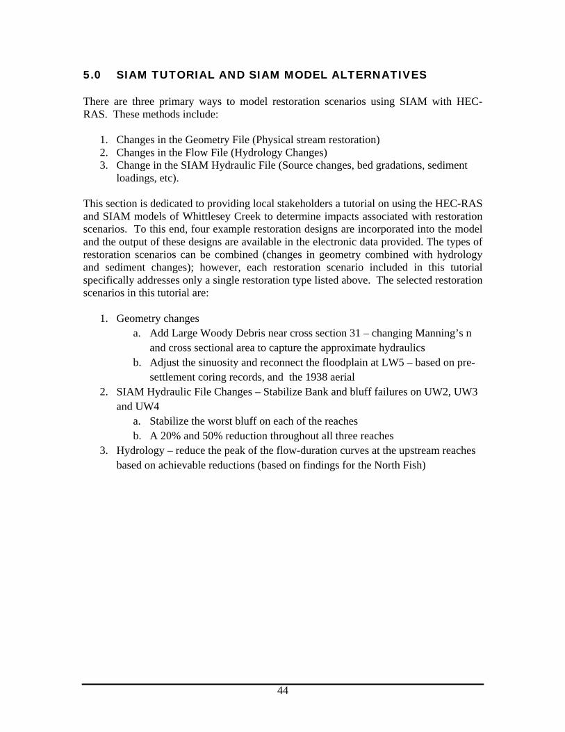
5.0 SIAM TUTORIAL AND SIAM MODEL ALTERNATIVES There are three primary ways to model restoration scenarios using SIAM with HEC-RAS. These methods include:

1. Changes in the Geometry File (Physical stream restoration) 2. Changes in the Flow File (Hydrology Changes) 3. Change in the SIAM Hydraulic File (Source changes, bed gradations, sediment

loadings, etc). This section is dedicated to providing local stakeholders a tutorial on using the HEC-RAS and SIAM models of Whittlesey Creek to determine impacts associated with restoration scenarios. To this end, four example restoration designs are incorporated into the model and the output of these designs are available in the electronic data provided. The types of restoration scenarios can be combined (changes in geometry combined with hydrology and sediment changes); however, each restoration scenario included in this tutorial specifically addresses only a single restoration type listed above. The selected restoration scenarios in this tutorial are:

1. Geometry changes a. Add Large Woody Debris near cross section 31 – changing Manning’s n

and cross sectional area to capture the approximate hydraulics b. Adjust the sinuosity and reconnect the floodplain at LW5 – based on pre-

settlement coring records, and the 1938 aerial 2. SIAM Hydraulic File Changes – Stabilize Bank and bluff failures on UW2, UW3

and UW4 a. Stabilize the worst bluff on each of the reaches b. A 20% and 50% reduction throughout all three reaches

3. Hydrology – reduce the peak of the flow-duration curves at the upstream reaches based on achievable reductions (based on findings for the North Fish)

45

5.1 Getting Started with SIAM

SIAM is accessed by selecting the Hydraulic Design Functions icon after opening and running the existing HEC-RAS model. The Hydraulic Design – Sediment Impact Assessment Model window was displayed. To begin establishing sediment reaches in the Hydraulic Design – Sediment Impact Assessment Model window Siam was checked under the Type drop down menu on the toolbar. Then File/ New Sediment Reach was selected on the toolbar to establish the first sediment reach. The active River and Reach were selected from the drop down boxes (automatically populated from the HEC-RAS model). For each River Reach, a Sediment Reach (Sed Reach) was given a name, an Upstream River Station (US RS) and Downstream River Station (DS RS) using the HEC-RAS model geometry profile and the following steps:

1. Select File/New Sediment Reach 2. The New Sediment Reach window was displayed 3. A name was entered for the new SIAM sediment reach, ie. NF1, for the first

sediment reach on North Fork Creek 4. OK 5. The upstream river station for the NF1 in the US RS drop-down box and the

downstream river station from the DS RS drop-down box were selected, forming the limits of the sediment reach.

6. After establishing each sediment reach File/Save Hydraulic Design Data was selected

7. A Filename was created for the hydraulic design data and a short id was entered to distinguish the file from any additional hydraulic design data files that might be created. The short id is the identifier in the Tables that were populated from computations in SIAM. (To create an additional hydraulic design data file with some of the same properties, File/Save Hydraulic Design Data As was used and the data was saved under another Filename and short id.)

8. OK Each sediment reach was given a Property Group name associated with it by selecting the Create a New Sediment Property Group icon, typing in a name, and selecting OK. Each sediment reach was given a Source Group name associated with it by selecting the Create a New Sediment Source Group icon, typing in a name, and selecting OK. Sediment source records were defined and edited by selecting the Define/Edit Sediment Sources button at the bottom of the template. An inset window appeared for source definition. Selecting the Create a New Sediment Source button, the source template was given a name and a source Type was selected from the drop-down box. For example the upland source for the first sediment reach on North Fork Creek was named NF1upland and the type was identified as Upstream erosion.

46

To view the input and interact with the output files for a pre-programmed restoration scenario (in this example the Large Woody Debris restoration scenario is selected) follow these steps: Step 1 Select the Perform Steady State Flow Simulation button on the main screen:

Step 2 Select File, then Open Plan, and select the Large Woody Debris Plan and click on OK:

Step 3 If a flow simulation has already been run (as in this example), then the user can close the Steady Flow Analysis window. Otherwise, the Compute button may be selected to perform the steady state flow simulation.

47

Step 4 Select the Perform Hydraulic Design Computation button from the HEC-RAS main screen:

Step 5 A window will appear asking the user to open a new Hydraulic Design (HD) file. Click on Yes:

Step 6 From the Open Hydraulic Design File window, select the Large Woody Debris hydraulic design file and click on OK:

It is recommended to close the Hydraulic Design File and reopen it so that the active HD file warning in Step 5 does not appear. This will clear all previous data from the Hydraulic Design file.

48

Step 7 The user may interact with the SIAM input files or view the output for the selected restoration scenario (in this case constructing large woody debris). Select the Tables button to view the output:

If changes to the geometry file, flow file, or hydraulic design file are made, the SIAM output can be updated by clicking on the Compute button, and then clicking on Apply.

49

Step 8 After selecting the Tables button, the user may view the output in a tabular or graphical form. The table is the default output and is viewed in the Tables tab. The Plot tab will display a graph of the sediment characteristics for each reach.

50

Additional tables and charts are available to view by selecting the Type in the Total Bed Material Budget window. Types include:

1. Total Bed Material Budget 2. Sediment Transport Potential by Flow and Grain Size 3. Supply and Balance 4. Several additional tables related to sediment characteristics by grain size

These steps can be followed to open any of the existing restoration scenarios that are pre-programmed into the SIAM model.

51

5.2 Large Woody Debris Restoration

Large woody debris is being designed and has been constructed in various locations throughout the watershed to provide habitat restoration and stabilize eroding banks (see Figure 24). Currently, a design is being considered that will add woody debris along a 2000 foot long reach just upstream of Ondossagon Road bridge. This corresponds to river stationing 2470 to 3040 in the Lower Whittlesey Reach (also corresponds to LW2 in the hydraulic design file). A conceptual design representative of this approach has been modeled in SIAM to determine impacts to the overall sediment dynamics of the Whittlesey Creek system. The files used in the Large Woody Debris design are shown in Table 15. Figure 24 – Constructed Large Woody Debris in the Upper Whittlesey Creek Reach

Table 15 – Files Associated with the Large Woody Debris Restoration Scenario File Description Plan WhittleseySIAM.p03 Large Woody Debris Geometry WhittleseySIAM.g02 Large Woody Debris Flow WhittleseySIAM.f05 Baseline Flow Hydraulic Design WhittleseySIAM.h01 Large Woody Debris

52

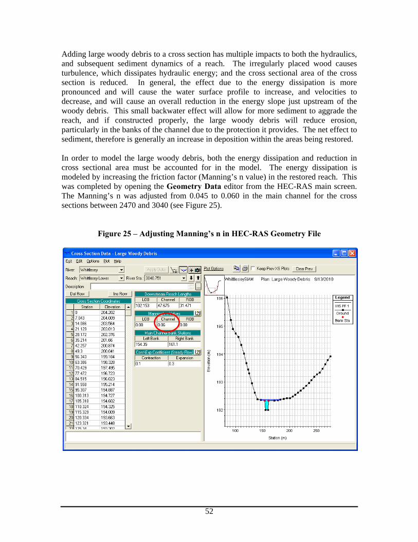
Adding large woody debris to a cross section has multiple impacts to both the hydraulics, and subsequent sediment dynamics of a reach. The irregularly placed wood causes turbulence, which dissipates hydraulic energy; and the cross sectional area of the cross section is reduced. In general, the effect due to the energy dissipation is more pronounced and will cause the water surface profile to increase, and velocities to decrease, and will cause an overall reduction in the energy slope just upstream of the woody debris. This small backwater effect will allow for more sediment to aggrade the reach, and if constructed properly, the large woody debris will reduce erosion, particularly in the banks of the channel due to the protection it provides. The net effect to sediment, therefore is generally an increase in deposition within the areas being restored. In order to model the large woody debris, both the energy dissipation and reduction in cross sectional area must be accounted for in the model. The energy dissipation is modeled by increasing the friction factor (Manning’s n value) in the restored reach. This was completed by opening the Geometry Data editor from the HEC-RAS main screen. The Manning’s n was adjusted from 0.045 to 0.060 in the main channel for the cross sections between 2470 and 3040 (see Figure 25).

Figure 25 – Adjusting Manning’s n in HEC-RAS Geometry File

53

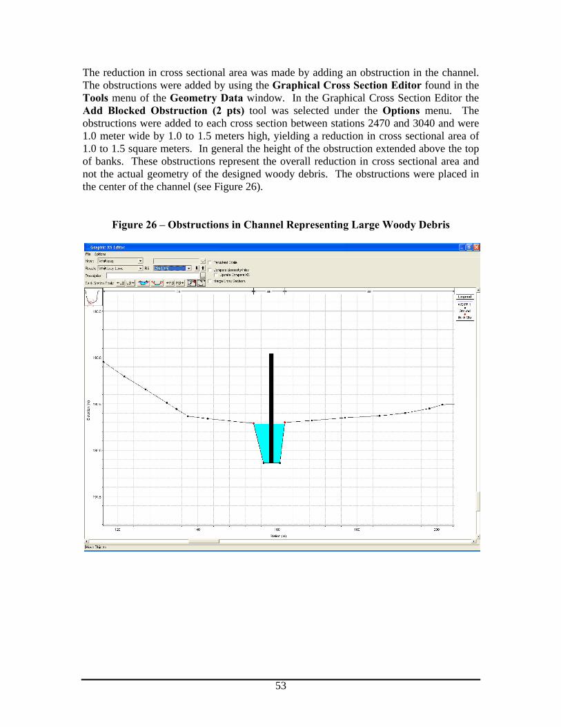
The reduction in cross sectional area was made by adding an obstruction in the channel. The obstructions were added by using the Graphical Cross Section Editor found in the Tools menu of the Geometry Data window. In the Graphical Cross Section Editor the Add Blocked Obstruction (2 pts) tool was selected under the Options menu. The obstructions were added to each cross section between stations 2470 and 3040 and were 1.0 meter wide by 1.0 to 1.5 meters high, yielding a reduction in cross sectional area of 1.0 to 1.5 square meters. In general the height of the obstruction extended above the top of banks. These obstructions represent the overall reduction in cross sectional area and not the actual geometry of the designed woody debris. The obstructions were placed in the center of the channel (see Figure 26).

Figure 26 – Obstructions in Channel Representing Large Woody Debris

54

The impacts associated with the addition of large woody debris to the sediment balance are available in the Tables of the SIAM output. Adding large woody debris to the LW2 sediment reach had impacts that extended both upstream and downstream of the restoration area. LW2 experienced increased deposition of sediment due to the decreased shear stresses associated with the flatter backwater slopes. Due to increased deposition in LW2, less sediment is carried to LW3 and since the overall sediment capacity of LW3 remained the same, net erosion resulted (in the Baseline case LW3 was a depositional reach). The excess sediment eroded from LW3 is then deposited in LW4, resulting in less erosion when compared to the baseline case. No impacts are realized downstream of LW4. The effects of a downstream alteration can extend a far distance upstream. In this case the addition of large woody debris impacted the hydraulics (water surface profile and velocities) in LW1 and UW6. See Table 16 and Figure 27 for detailed results of this analysis.

55

Table 16 – Sediment Impacts from Large Woody Debris

Reach 

Baseline Sediment 

Balance, tons per year 

Large Woody Debris  

Sediment Balance, tons 

per year  Difference  Description 

NF1  ‐6123  ‐6123 0  No Change 

NF2  ‐15800  ‐15800 0  No Change 

NF3  17700  17700 0  No Change 

UW1  ‐3241  ‐3241 0  No Change 

UW2  ‐362  ‐362 0  No Change 

UW3  ‐254  ‐254 0  No Change 

UW4  ‐2146  ‐2146 0  No Change 

UW5  ‐2606  ‐2606 0  No Change 

UW6  5488  5380 ‐108  Decrease Aggregation 

LW1  ‐25500  ‐25300 200  Decrease Erosion 

LW2  21100  28000 6900  Increase Aggregation 

LW3  2394  ‐5338 ‐7732  Aggregation to Erosion 

LW4  ‐47300  ‐46700 600  Decrease Erosion 

LW5  49300  49300 0  No Change 

LW6  5835  5835 0  No Change 

Figure 27 - Sediment Impacts from Large Woody Debris

‐60000

‐40000

‐20000

0

20000

40000

60000

NF1

NF2

NF3

UW1

UW2

UW3

UW4

UW5

UW6

LW1

LW2

LW3

LW4

LW5

LW6

Sedim

ent Balan

ce, tons/year

Baseline Large Woody Debris

Location of LWD in Model

56

5.3 Floodplain Reconnection in LW5

A second restoration scenario being considered consists of restoring the former floodplain and channel pattern within the Whittlesey Creek National Wildlife Refuge. In 1949, USACE straightened the channel from Cherryville Road to the mouth. This reduced the overall channel length by 900 feet and caused significant sedimentation and geomorphic evolution in the channel. In 2006 the USGS digitized the historical channels, shorelines, and deltas in order to determine the pre-straightened channel pattern (Figure 28). In addition, core samples were taken to determine floodplain elevations.

Figure 28 – Digitization of Historic Channel, Shorelines, and Deltas (USGS, 2006)

This restoration alternative seeks to restore the Lower Whittlesey Reach from station 874 to 1533. The files used for this restoration scenario are listed in Table 17.

57

Table 17 – HEC-RAS Files for the Floodplain Connection in LW5 Restoration File Description Plan WhittleseySIAM.p04 LW5 Floodplain Connection Geometry WhittleseySIAM.g03 LW5 Floodplain Connection Flow WhittleseySIAM.f05 Baseline Flow Hydraulic Design WhittleseySIAM.h03 LW5 Floodplain Connection

Similar to the large woody debris restoration option, this scenario required a change to the baseline geometry file. The USGS found approximately 1 to 2 meters of sedimentation based on the sediment cores within LW5. The geometry associated with the restored cross sections were edited using the Graphical Cross Section Editor. Floodplain elevations were restored to the former sediment depth. See Figure 29 for an example of the changes to the cross section geometry at station 15+33.

Figure 29 – Reconnected Floodplain at Station 15+33

In addition to the floodplain reconnection, an increased sinuosity (and subsequent decrease in channel slope) was introduced in this restoration scenario. This was accomplished by adding a total of 900 feet of channel length to the cross sections in LW5. The length added to each cross section was weighted based on the baseline channel length, and changes were made in the Cross Section Data window for each cross section (Figure 30).

185

185.5

186

186.5

187

187.5

188

188.5

189

189.5

0 20 40 60 80 100 120 140 160

Baseline Model Reconnected Floodplain

58

Figure 30 – Updated Channel Lengths to Reflect Increase Sinuosity (Station 15+33)

The SIAM results of this scenario show that deposition in the LW5 sediment reach is expected to decrease following the reconnection of the former floodplain. Since SIAM calculates sediment capacity in the channel, the reduction in channel cross section reduces capacity and subsequently reduces deposition. It should be noted however, that much of this sediment deposition reduction in the channel would be offset by an increased sediment deposition in the floodplain. The decrease in deposition in LW5 also contributes to an increase in deposition in the LW6 sediment reach. Since deposition is decreased in LW5, more sediment is expected to be transported to LW6. The transport capacity is unaffected in LW6, and therefore the increase in bed supply from LW5 results in more sedimentation in the LW6 reach. This unintended consequence could adversely affect spawning habitat in the LW6 reach. Detailed results are displayed in Table 18 and Figure 31.

59

Table 18 – Sediment Impacts from LW5 Floodplain Connection

Reach 

Baseline Sediment 

Balance, tons per year 

LW5 Floodplain Connection Sediment 

Balance, tons per year  Difference  Description 

NF1  ‐6123  ‐6178  ‐55  No Change (model uncertainty) 

NF2  ‐15800  ‐15800  0  No Change 

NF3  17700  17700  0  No Change 

UW1  ‐3241  ‐3241  0  No Change 

UW2  ‐362  ‐362  0  No Change 

UW3  ‐254  ‐254  0  No Change 

UW4  ‐2146  ‐2146  0  No Change 

UW5  ‐2606  ‐2606  0  No Change 

UW6  5488  5488  0  No Change 

LW1  ‐25500  ‐25500  0  No Change 

LW2  21100  21100  0  No Change 

LW3  2394  2394  0  No Change 

LW4  ‐47300  ‐45200  2100  Decrease Erosion 

LW5  49300  44900  ‐4400  Decrease Aggradation 

LW6  5835  8106  2271  Increased Aggradation 

Figure 31 - Sediment Impacts from LW5 Floodplain Connection

‐60000

‐40000

‐20000

0

20000

40000

60000

NF1

NF2

NF3

UW1

UW2

UW3

UW4

UW5

UW6

LW1

LW2

LW3

LW4

LW5

LW6

Sedim

ent Balan

ce, tons/year

Baseline LW5 Floodplain Connection

60

5.4 Reduced Peak Flows

The next restoration option consists of a scenario where the steady flow file is modified in HEC-RAS. This reflects a hydrologic change in the watershed and could be the result of precipitation change, landuse, or implementation of Best Management Practices (BMPs). In this example, it is assumed that detention basins and wetland restoration BMPs are implemented in the upper North Fork Reach (NF1 and NF2) and the Upper Whittlesey Creek Reach (UW1). These BMPs will result in reduced peak flows in the upper reaches of the watershed. Files associated with the reduced peak flow restoration option are shown in Table 19.

Table 19 - HEC-RAS Files for the Reduced Peak Flow Restoration File Description Plan WhittleseySIAM.p02 Reduced Peak Flows Geometry WhittleseySIAM.g01 Baseline Geometry Flow WhittleseySIAM.f02 Reduced Peak Flows Hydraulic Design WhittleseySIAM.h02 Reduced Peak Flows

To model the impacts to the sediment dynamics following the implementation of detention and wetland BMPs, the achievable reduction in peak flows must first be determined. The hydrologic changes associated with the BMPs have not been modeled in detail for the Whittlesey Creek. However, a detailed hydrologic model of the nearby Fish Creek has been completed (Blodgett, 2009). This study focused on determining the impacts that detention and wetland restoration has on upland runoff attenuation in the North Fish Creek watershed. The Blodgett study concluded that peak flow reductions of 25% to 40% can be realized through the construction of detention basins with 20-200 acre-feet of storage, combined with wetland restoration. Similar reductions to peak flows have been assumed and applied to the Whittlesey Creek steady flow file. Since detention BMPs will generally not significantly affect baseflow, only the peak discharges are assumed to be reduced by 40%. Moreover, it is assumed that bankfull flows can be reduced by up to 25%. Table 20 shows the reduction in flow for NF1, NF2, and UW1 steady flow files.

61

Table 20 – Steady Flow File Percent Reductions for NF1, NF2, and UW1

Profile Percent Reduction PF1 0% PF2 0% PF3 0% PF4 25% PF5 25% PF6 25% PF7 40% PF8 40% PF9 40% PF10 40%

The steady flow file was modified by opening the Steady Flow Data Editor from the HEC-RAS main screen. Figure 32 shows the flow values used in this restoration scenario. Note that this does not assume any propagation of the flow reduction to downstream reaches. A detailed hydrology model may be used to more accurately determine the impacts to adjacent reaches and the overall system following the implementation of detention basins and wetland restoration.

Figure 32 – Flows Used in the Reduced Peak Flow Restoration Scenario

Overall, the results of reducing the peak flows by 40% and bankfull flows by 25% had little effect to the sediment dynamics of the system. Sediment erosion typically decreased by 1-3% in the upper reaches, and had little effect to downstream reaches. The results of modeling this scenario are shown in Table 21 and Figure 33.

62

Table 21 – Sediment Impacts from Reducing Peak Flows in Upper Reaches

Reach 

Baseline Sediment 

Balance, tons per year 

Reduced Peak Flows 

Sediment Balance, tons 

per year  Difference  Description 

NF1  ‐6123  ‐4550 1573  Decrease Erosion 

NF2  ‐15800  ‐16000 ‐200  Decrease Erosion 

NF3  17700  16300 ‐1400  Decrease Aggredation 

UW1  ‐3241  ‐3075 166  Decrease Erosion 

UW2  ‐362  ‐528 ‐166  Increase Erosion 

UW3  ‐254  ‐254 0  No Change 

UW4  ‐2146  ‐2146 0  No Change 

UW5  ‐2606  ‐2606 0  No Change 

UW6  5488  5488 0  No Change 

LW1  ‐25500  ‐25500 0  No Change 

LW2  21100  21100 0  No Change 

LW3  2394  2394 0  No Change 

LW4  ‐47300  ‐47300 0  No Change 

LW5  49300  49300 0  No Change 

LW6  5835  5836 1  No Change (model uncertainty) 

Figure 33 - Sediment Impacts from Reducing Peak Flows in Upper Reaches

‐60000

‐40000

‐20000

0

20000

40000

60000

NF1

NF2

NF3

UW1

UW2

UW3

UW4

UW5

UW6

LW1

LW2

LW3

LW4

LW5

LW6

Sedim

ent Balan

ce, tons/year

Baseline Reduced Peak Flow

63

5.5 Bank Stabilization

The last restoration scenario modeled as part of this tutorial address the reduction of the source loadings from the banks of the river at selected locations. This type of restoration only changes the Hydraulic Design file (no changes are made to the geometry file or the flow file). The focus of this scenario is to stabilize a portion of the banks on UW2, UW3, and UW4. First, the effect of stabilizing the worst eroding bank will be determined. Next, stabilizing 50% of the total banks contributing sediment to these three reaches will be modeled. The files used in this analysis are shown in Table 22.

Table 22 - HEC-RAS Files for the Bank Stabilization Restoration Scenario File Description Plan WhittleseySIAM.p05 Bank Stabilization UW2,

UW3, UW4 Geometry WhittleseySIAM.g01 Baseline Geometry Flow WhittleseySIAM.f05 Baseline Flow Hydraulic Design WhittleseySIAM.h04 Bank Stabilization UW2,

UW3, UW4 The USGS collected bank erosion data in 2006 throughout the watershed. The eroding banks identified within these three reaches are described in Table 23.

64

Table 23 – Bank Erosion Data Collected by USGS, 2006

USGS SiteID

SIAM Station

SIAM Reach

Bank height or height of

erosion (ft)

length of

eroding bank (ft)

est. bank

retreat (ft)

est bank erosion volume

(ft3)

Bank Erosion

tons

27.6  6324  UW4  30  40  5  6,000  255 

35.1 6927 UW4 10 150 6 9,000  382.5 

37.6  7395  UW3  10  20  3  600  25.5 

37.7  7395  UW3  8  30  3  720  30.6 

40.1  7453  UW3  6  40  2  480  20.4 

40.2  7453  UW3  10  50  1  500  21.25 

40.3  7507  UW3  20  60  2  2,400  102 

41.2  7563  UW3  6  20  3  360  15.3 

42.1  7774  UW3  5  50  3  750  31.875 

43.2  8008  UW3  20  90  5  9,000  382.5 

43.5  8008  UW3  12  120  5  7,200  306 

45.0  8180  UW3  25  70  5  8,750  371.875 

45.0  8180  UW3  20  20  5  2,000  85 

46.0  8180  UW3  15  200  5  15,000  637.5 

47.0  8344  UW3  15  5  5  375  15.9375 

48.0  8344  UW3  10  50  5  2,500  106.25 

49.0  8500  UW3  18  100  5  9,000  382.5 

50.0  8634  UW3  4  400  2  3,200  136 

51.0  8634  UW3  50  50  3  7,500  318.75 

51.0  8634  UW3  10  100  5  5,000  212.5 

51.0  8634  UW3  4  400  2  3,200  136 

52.0  8864  UW2  10  200  3  6,000  255 

53.0  8864  UW2  10  50  3  1,500  63.75 

54.0  9077  UW2  40  50  5  10,000  425 

55.0  9077  UW2  10  100  5  5,000  212.5 

56.0  9227  UW2  40  50  5  10,000  425 

56.0  9227  UW2  10  50  3  1,500  63.75 

57.0  9227  UW2  30  200  5  30,000  1275 

58.0  9667  UW2  4  200  5  4,000  170 

59.0  9370  UW2  10  100  5  5,000  212.5 

60.0  9370  UW2  10  200  4  8,000  340 

61.0  9777  UW2  10  200  4  8,000  340 

63.0  9926  UW2  10  200  4  8,000  340 

65.5  9980  UW2  10  50  3  1,500 63.75 

65.6  10125  UW2  9  50  4  1,800 76.5 

65.7  10125  UW2  40  50  5  10,000 425 

65

USGS SiteID

SIAM Station

SIAM Reach

Bank height or height of

erosion (ft)

length of

eroding bank (ft)

est. bank

retreat (ft)

est bank erosion volume

(ft3)

Bank Erosion

tons

65.8  10125  UW2  9  70  5  3,150  133.875 

66.9  10125  UW2  3  100  2  600  25.5 

66.9  10125  UW2  10  30  3  900  38.25 

67.1  10237  UW2  30  100  5  15,000  637.5 

67.8  10237  UW2  4  500  1  2,000  85 

69.5  10237  UW2  8  2  2  32  1.36 

69.5  10237  UW2  5  700  2  7,000  297.5 

69.6  10237  UW2  12  12  2  288  12.24 

69.7  10359  UW2  10  20  4  800  34 

69.9  10359  UW2  75  90  1  6,750  286.875 

70.0  10359  UW2  5  20  1  100  4.25 

70.3  10359  UW2  20  20  1  400  17 

70.2  10359  UW2  15  25  2  750  31.875 

70.1  10359  UW2  75  45  1  3,375  143.44 

71.5  10359  UW2  20  100  5  10,000  425 

71.5  10359  UW2  3  500  3  4,500  191.25 

The first impact analysis on bank stabilization on these reaches consists of stabilizing the worst bank on each of the three reaches. SIAM provides a loading multiplier for each source loading, and therefore, the percent reduction of bank/bluff erosion may be calculated and input as a multiplier in the model. A summary of the bank and bluff erosion data is provided in Table 24, which also determines the overall percent reduction achieved for stabilizing the worst bank on each of the three reaches.

Table 24 – Summary of Bank Erosion Data for UW2, UW3, and UW4

Reach 

Location of Largest 

Contributing Bank 

Bank Erosion at Largest 

Contributing Bank, ft3 

Bank Erosion at Largest 

Contributing Bank, tons 

Total Bank Erosion for Entire Reach, 

tons 

Percent of Total Bank Erosion for 

Reach 

UW2  9226.75  30000  1275  7052.7  18.1% 

UW3  8180.395  15000  637.5  3337.7  19.1% 

UW4  6927.225  9000  382.5  637.5  60.0% 

The source loadings can be updated by opening the Hydraulic Design File. In the WhittleseySIAM.h04 design file, the bank inputs of sediment can be updated by adjusting the multiplier in the Source Loading tab. Based on the calculated percent

66

reductions in Table X, the multiplier assigned to the bank/bluff/gully component of UW2, UW3, and UW4 is 0.819, 0.809, and 0.60 respectively. See Figure 34 for an example.

Figure 34 – Location of Sources Multiplier for Bank/Bluff/Gully Loading

The results of the bank stabilization analysis show that there is little effect on the sediment aggradation or erosion potential throughout the system. When compared to the bed supply, the source loadings associated with a single bank are very small. Although the banks make up a large portion of the sediment budget, much of the sediment is stored in the channel as legacy sediments, and therefore the bed supply dominates the SIAM output. The results show that stabilizing the worst banks in these three reaches will result in slightly increased erosion in UW2 and UW4 due to reduced sediment loading while maintaining the same transport capacity. This analysis also shows that a decrease in deposition will occur in UW3 due to a reduction in the loading in a depositional reach. The results are shown in Table 25 and Figure 35. Improvements to the stream morphology will not be realized until the legacy sediments associated with previous bank failures have been transported through the system and a stable river morphology is reached.

67

Table 25 – Sediment Impacts from Stabilizing the Worst Banks on UW3-5

Reach 

Baseline Sediment 

Balance, tons per year 

Stabilizing Worst Banks Sediment 

Balance, tons per year  Difference  Description 

NF1  ‐6123  ‐6123  0  No Change 

NF2  ‐15800  ‐15800  0  No Change 

NF3  17700  17700  0  No Change 

UW1  ‐3241  ‐3241  0  No Change 

UW2  ‐362  ‐364  ‐2  Small Increase Erosion 

UW3  ‐254  ‐297  ‐43  Small Increase Erosion 

UW4  ‐2146  ‐2215  ‐69  Small Increase Erosion 

UW5  ‐2606  ‐2606  0  No Change 

UW6  5488  5488  0  No Change 

LW1  ‐25500  ‐25500  0  No Change 

LW2  21100  21100  0  No Change 

LW3  2394  2394  0  No Change 

LW4  ‐47300  ‐47300  0  No Change 

LW5  49300  49300  0  No Change 

LW6  5835  5835  0  No Change 

Figure 35 - Sediment Impacts from Stabilizing the Worst Bank on UW3-5

‐60000

‐40000

‐20000

0

20000

40000

60000

NF1

NF2

NF3

UW1

UW2

UW3

UW4

UW5

UW6

LW1

LW2

LW3

LW4

LW5

LW6

Sedim

ent Balan

ce, tons/year

Baseline Stabilize Worst Bank

68

The stabilization analysis was repeated with a scenario that looked at stabilizing 50% of the banks within UW3, UW4, and UW5. Again, the multiplier associated with the bank/bluff/gully component on the source loadings was adjusted, this time to 0.50 for each of the three reaches. Similar results were obtained, which showed only small impacts to the immediate reaches being restored. The largest impact was a reduction in deposition potential by 114 tons per year in UW3. Erosion potential again increased in both UW2 and UW4 due to the reduction in sediment loads without a change to the sediment transport capacity. Results for the 50% stabilization scenario are shown in Table 26 and Figure 36.

Table 26 – Sediment Impacts from Reducing Bank Erosion by 50% on UW3-5

Reach 

Baseline Sediment 

Balance, tons per year 

50% Bank Stabilization Sediment 

Balance, tons per year  Difference  Description 

NF1  ‐6123  ‐6123  0  No Change 

NF2  ‐15800  ‐15800  0  No Change 

NF3  17700  17700  0  No Change 

UW1  ‐3241  ‐3241  0  No Change 

UW2  ‐362  ‐366  ‐4  Small Increase Erosion 

UW3  ‐254  ‐368  ‐114  Small Increase Erosion 

UW4  ‐2146  ‐2203  ‐57  Small Increase Erosion 

UW5  ‐2606  ‐2606  0  No Change 

UW6  5488  5488  0  No Change 

LW1  ‐25500  ‐25500  0  No Change 

LW2  21100  21100  0  No Change 

LW3  2394  2394  0  No Change 

LW4  ‐47300  ‐47300  0  No Change 

LW5  49300  49300  0  No Change 

LW6  5835  5835  0  No Change 

69

Figure 36 - Sediment Impacts from Reducing Bank Erosion by 50% on UW3-5

‐60000

‐40000

‐20000

0

20000

40000

60000

NF1

NF2

NF3

UW1

UW2

UW3

UW4

UW5

UW6

LW1

LW2

LW3

LW4

LW5

LW6

Sedim

ent Balan

ce, tons/year

Baseline 50% Stabilize on All Three Banks

70

5.6 Additional Restoration Scenarios and Model Limitations

The previous examples show how the SIAM model can be used to analyze the impacts to the deposition or erosion potential of the Whittlesey Creek system under a variety of restoration scenarios. These examples independently looked at the impacts of adjusting one of the three types of files used in a SIAM analysis (Geometry, Flow, and Hydraulic Design files). The user may combine some of the restoration scenarios by creating a new plan and selecting the files used in that plan. For instance, the impacts following construction of large woody debris and detention basins could be analyzed by creating a plan that uses the Large Woody Debris geometry file and the Reduced Peak flow file. The Whittlesey Creek SIAM model has been designed as a screening tool to prioritize restoration options within the watershed. Using the guidance provided in this tutorial section, the user is equipped to adjust flow data, geometry data, or source loading data. This will be useful to prioritize restoration scenarios based on the overall impacts to the Whittlesey Creek watershed and to identify unintended consequences of a restoration conceptual design. Once a restoration scenario is identified through the screening process that SIAM provides, it is recommended that a more detailed model, such as a sediment routing model, be used to calculate erosion and deposition rates in specific reaches. The values that SIAM provides are erosion and deposition potential, and the results should not be used for detailed design purposes. SIAM does not route sediment, nor does it allow for cross sections to be updated following sediment deposition or erosion. When used for its intended purpose of screening restoration scenarios, SIAM is a powerful tool that can save significant time and money by focusing on the most feasible approaches to watershed and river restoration.

71

6.0 SUMMARY AND CONCLUSIONS The US Army Corps of Engineers partnered with the US Fish and Wildlife Service and the US Geological Survey and studied the sedimentation and erosion potential of the Whittlesey Creek watershed. A number of restoration plans are being considered within the watershed, and much of the restoration is motivated by the goals and objectives of the Whittlesey Creek National Wildlife Refuge. This project supports those goals, particularly to restore Coaster Brook Trout within the Wildlife Refuge. The Sediment Impact Analysis Methods (SIAM) model was developed to be used as a screening tool in selecting appropriate restoration options. Four restoration options have been modeled as part of this study. These range from floodplain reconnection in the lower reaches of the watershed, bank stabilization, peak flow reduction through the construction of detention basins and wetland restoration in the upper reaches, and the construction of large woody debris. Peak flow reduction in the upper reaches reduced the total transport capacity within the upper reaches, and therefore less sediment is expected to be mobilized. However, positive impacts are quickly attenuated downstream because the transport capacity of the lower reaches was not significantly changed. Floodplain reconnection promoted sedimentation in the reconnected floodplain; however, this negatively impacted downstream reaches by reducing sediment loading and causing the most downstream reach to become an eroding reach. It is recommended that if floodplain connection is considered, that the connection extends to the delta area so that the entire lower two reaches become depositional during peak events. Bank stabilization was shown to have the least effect on the sedimentation and erosion of the entire system. This is because most of the sediment in the system is currently stored in the channel (point bars, bed, mid channel bars, and plugged reaches). Since the banks have been contributing sediment significantly since logging, the total sediment that has been mobilized and currently stored in the system is large. On an annual basis, the stabilization of a single bank will not greatly affect the system until the stored sediment is permanently deposited in a depositional reach. The construction of large woody debris was shown to have a significant effect to both upstream reaches and downstream reaches. The reach where large woody debris is implemented typically increased deposition due to the velocity and shear stress reduction associated with the backwater profile behind the large woody debris. Moreover, upstream reaches were affected by the backwater, which may extend a far distance upstream. Downstream reaches are affected because the sediment that deposited in the reach associated with the large woody debris becomes unavailable for transport, but the transport capacity of the reach is unaffected. This generally caused an increase in erosion of the downstream reaches. It is recommended that large woody debris be analyzed more closely with a sediment transport model to determine the potential magnitude of these designs.

72

Most restoration scenarios have multiple objectives, and the effects of sediment is often not the driving reason to motivate restoration. However, the interrelated impacts to sediment, hydraulics, and river morphology should be considered in all restoration designs. The analysis provided by SIAM for Whittlesey Creek can both determine the interrelated impacts of combined restoration scenarios, and determine if a downstream restoration will be filled by upstream sediment moving through the system or eroded due to the changes in the hydraulics of the restored reach. This powerful tool will allow local stakeholders to focus restoration efforts and money to the most feasible projects that have the greatest chance for long-term restoration success.

73

REFERENCES Blodgett, D., 2009. Modeling Flood Flow Reduction for Bluff Erosion Mitigation using

Upland Runoff Attenuation on North Fish Creek, Bayfield County, WI. University of Wisconsin-Madison Master of Science Thesis in Water Resources Engineering.

Hydrologic Engineering Center. HEC-RAS User’s Manual, U.S. Army Corps of

Engineers, Davis, CA, 2008. Hydrologic Engineering Center. HEC-RAS River Analysis System Hydraulic Reference

Manual, U.S. Army Corps of Engineers, Davis, CA, 2008. Lenz BN, Saad DA, Fitzpatrick FA. 2003. Simulation of Ground-Water Flow and

Rainfall Runoff with Emphasis on the Effects of Land Cover, Whittlesey Creek, Bayfield County, Wisconsin, 1999-2001. US Geological Survey Water-Resources Investigations Report 03-4130, 47 p.

Rose, W., and Graczyk, D., 1996, Sediment transport, particle size, and loads in North

Fish Creek in Bayfield County, Wisconsin, water years 1990–91: U.S. Geological Survey Water-Resources Investigations Report 95–4222, 18 p.

Wisconsin Department of Natural Resources, 1996. A nonpoint source control plan for

the Whittlesey Creek Priority Watershed Project: Wisconsin Department of Natural Resources Publication WR-474-96, 55 p.

A-1

APPENDIX A BED MATERIAL GRADATIONS

A-2

0

10

20

30

40

50

60

70

80

90

100

0.01 0.1 1 10 100 1000

% Finer

Particle Diameter (mm)

North Fork ‐ Reach 1

BedNF1pc

0

10

20

30

40

50

60

70

80

90

100

0.01 0.1 1 10 100 1000

% Finer

Particle Diameter (mm)

North Fork ‐ Reach 2

BedNF2pc BedNF2int40 BedNF2int41 BedNF2faf

A-3

0

10

20

30

40

50

60

70

80

90

100

0.01 0.1 1 10 100 1000

% Finer

Particle Diameter (mm)

North Fork ‐ Reach 3

BedNF3pc BedNF3int

A-4

0

10

20

30

40

50

60

70

80

90

100

1 10 100

% Finer

Particle Diameter (mm)

Upper Whittlesey ‐ Reach 1

BedUW1pc BedUW1faf

0

20

40

60

80

100

1 10 100

% Finer

Particle Diameter (mm)

Upper Whittlesey ‐ Reach 2

BedUW2st20 BedUW2st13 BedUW2st20r

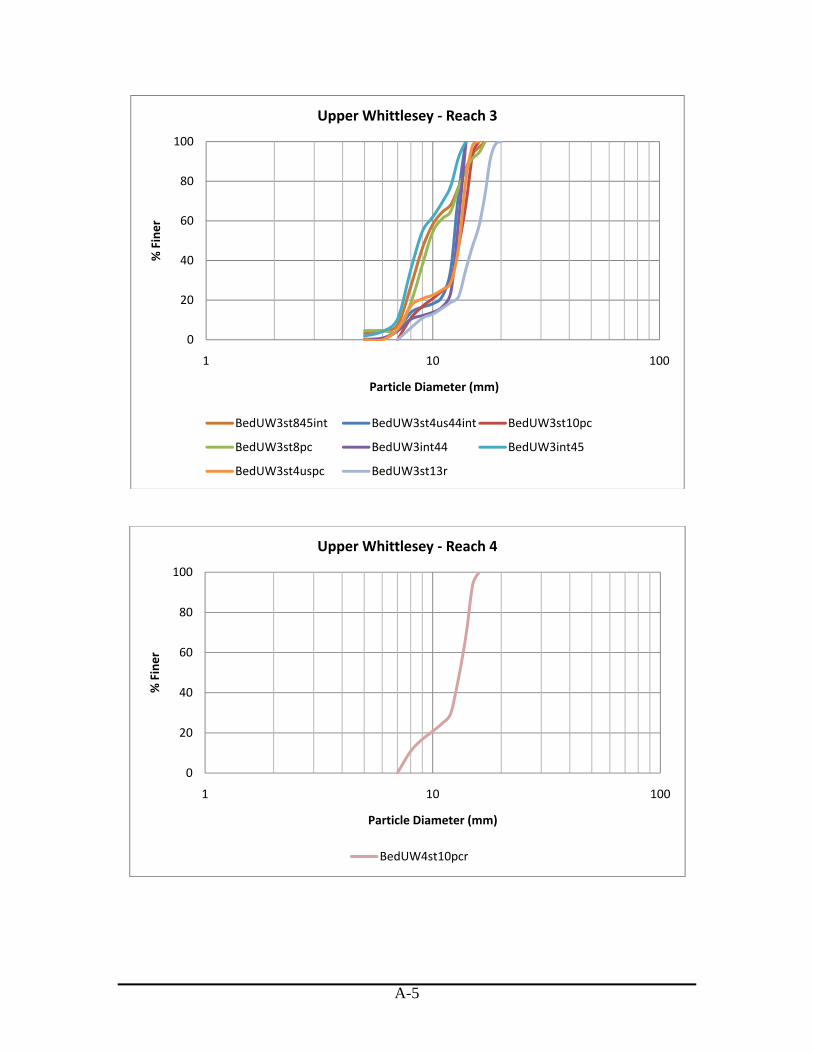
A-5

0

20

40

60

80

100

1 10 100

% Finer

Particle Diameter (mm)

Upper Whittlesey ‐ Reach 3

BedUW3st845int BedUW3st4us44int BedUW3st10pc

BedUW3st8pc BedUW3int44 BedUW3int45

BedUW3st4uspc BedUW3st13r

0

20

40

60

80

100

1 10 100

% Finer

Particle Diameter (mm)

Upper Whittlesey ‐ Reach 4

BedUW4st10pcr

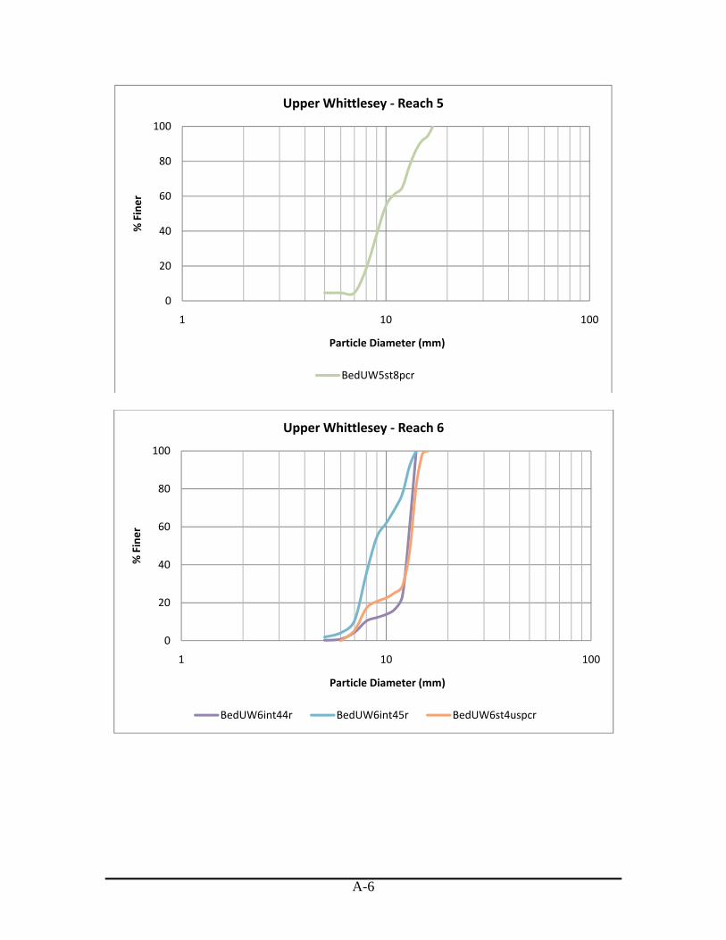
A-6

0

20

40

60

80

100

1 10 100

% Finer

Particle Diameter (mm)

Upper Whittlesey ‐ Reach 5

BedUW5st8pcr

0

20

40

60

80

100

1 10 100

% Finer

Particle Diameter (mm)

Upper Whittlesey ‐ Reach 6 

BedUW6int44r BedUW6int45r BedUW6st4uspcr

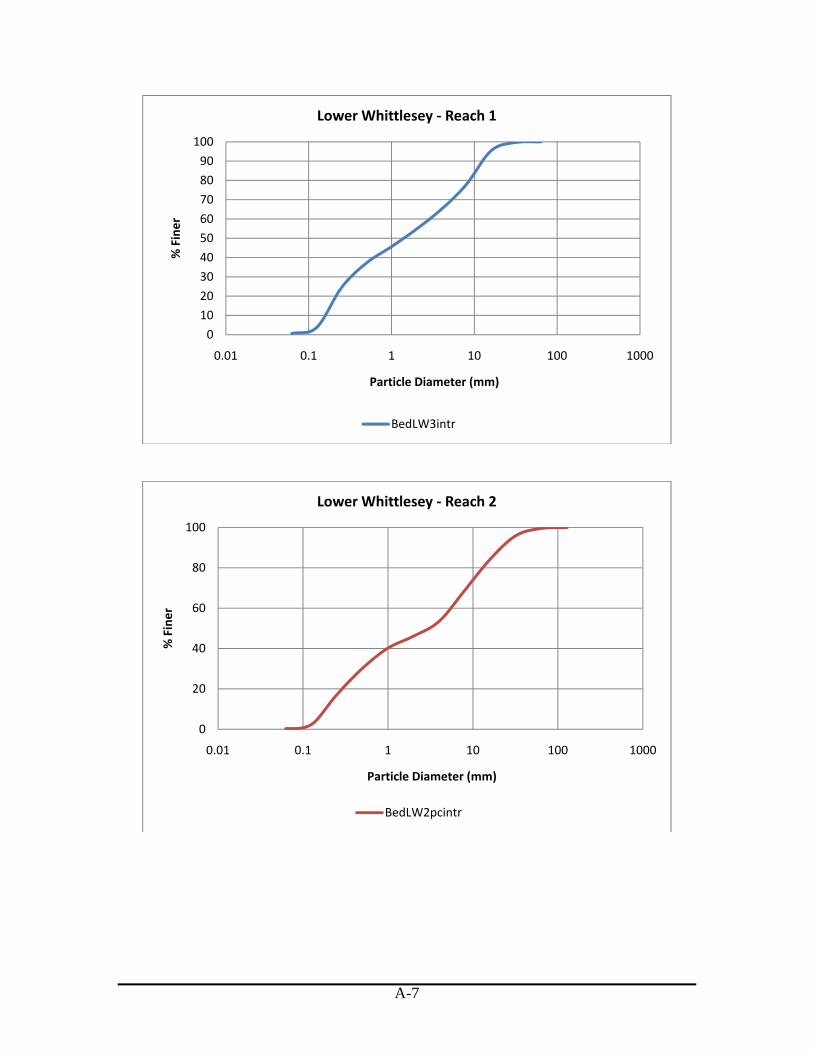
A-7

0

10

20

30

40

50

60

70

80

90

100

0.01 0.1 1 10 100 1000

% Finer

Particle Diameter (mm)

Lower Whittlesey ‐ Reach 1

BedLW3intr

0

20

40

60

80

100

0.01 0.1 1 10 100 1000

% Finer

Particle Diameter (mm)

Lower Whittlesey ‐ Reach 2

BedLW2pcintr

A-8

0

20

40

60

80

100

0.01 0.1 1 10 100 1000

% Finer

Particle Diameter (mm)

Lower Whittlesey ‐ Reach 3

BedLW3intr

0

10

20

30

40

50

60

70

80

90

100

1 10 100

% Finer

Particle Diameter (mm)

Lower Whittlesey ‐ Reach 4 

BedLW4intr BedLW4intrfaf

A-9

0

20

40

60

80

100

1 10 100

% Finer

Particle Diameter (mm)

Lower Whittlesey ‐ Reach 5

BedLW5intr

0

10

20

30

40

50

60

70

80

90

100

1 10 100

% Finer

Particle Diameter (mm)

Lower Whittlesey ‐ Reach 6

BedLW6intr