Whiteboard It!Convert Whiteboard Content into an Electronic Document

Zhengyou Zhang Li-wei HeMicrosoft Research

Email: zhang@microsoft.com, lhe@microsoft.com

Aug. 12, 2002

Abstract

This ongoing project aims at converting the content on a physical whiteboard, captured by a digitalcamera, into an electronic document which can be easily manipulated as drawings in a MS Office docu-ment or as inks in a TabletPC. Through a series of image processing procedures, the originally capturedimage is first transformed into a rectangular bitmap with clean white background, and finally convertedinto a vectorized representation (inks).

Contents

1 Introduction 2

2 Overview 2

3 Automatic Whiteboard Detection 33.1 Technical Details . . . . . . . . . . . . . . . . . . . . . . . . . . . . . . . . . . . . . . . 33.2 Experiments With Automatic Whiteboard Rectification . . . . . . . . . . . . . . . . . . . 4

4 Estimating Pose and Aspect Ratio of a Rectangular Shape from One Image, and the Camera’sFocal Length 84.1 Geometry of a Rectangle . . . . . . . . . . . . . . . . . . . . . . . . . . . . . . . . . . . 84.2 Estimating Camera’s Focal Length and Rectangle’s Aspect Ratio . . . . . . . . . . . . . . 104.3 Experimental Results on Aspect Ratio Estimation . . . . . . . . . . . . . . . . . . . . . . 11

5 Rectification 12

6 White Balancing 13

7 Examples 13

8 Competitive Product 13

9 Technical Challenges 15

1

1 Introduction

A whiteboard provides a large shared space for collaboration among knowledge workers. It is not onlyeffective but also economical and easy to use – all you need is a flat board and several dry-ink pens. Whilewhiteboards are frequently used, they are not perfect. The content on the whiteboard is hard to archiveor share with others who are not present in the session. Our system aims at reproducing the whiteboardcontent as a faithful, yet enhanced and easily manipulable, electronic document through the use of a digitalcamera. It uses a series of image processing algorithms to clip the borders, rectify the whiteboard imagesand correct the colors.

2 Overview

Image Capture

Quadrangle Localization

Aspect Ratio Estimation

Image Rectification

White balancing of Background color

Image vector ization(“ Inkization” )

MS Office

TabletPCInks

Figure 1: System architecture

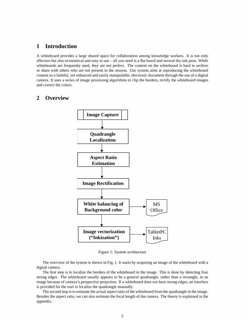
The overview of the system is shown in Fig. 1. It starts by acquiring an image of the whiteboard with adigital camera.

The first step is to localize the borders of the whiteboard in the image. This is done by detecting fourstrong edges. The whiteboard usually appears to be a general quadrangle, rather than a rectangle, in animage because of camera’s perspective projection. If a whiteboard does not have strong edges, an interfaceis provided for the user to localize the quadrangle manually.

The second step is to estimate the actual aspect ratio of the whiteboard from the quadrangle in the image.Besides the aspect ratio, we can also estimate the focal length of the camera. The theory is explained in theappendix.

2

The third step is image rectification. From the estimated aspect ratio, and by choosing the “largest”whiteboard pixel as the standard pixel in the final image, we can compute the desired resolution of thefinal image. A planar mapping (a 3× 3 homography matrix) is then computed from the original imagequadrangle to the final image rectangle, and the whiteboard image is rectified accordingly.

The fourth step is white balancing of the background color. This involves two procedures. The firstis the estimation of the background color (the whiteboard color under perfect lighting without anythingwritten on it). This is not a trivial task because of complex lighting environment, whiteboard reflection andstrokes written on the board. The second concerns the actual white balancing. We make the backgrounduniformly white and increase color saturation of the pen strokes. The output is a crisp image ready to beintegrated with any office document.

The fifth step is image vectorization. It transforms a bitmap image into vector drawings such as free-form curves, lines and arcs. TabletPC inks use a vector representation, and therefore a whiteboard imageafter vectorization can be exported into TabletPC.

Note that at the time of this writing, we have not yet implemented the vectorization step.

3 Automatic Whiteboard Detection

As was mentioned in the introduction, this work was motivated by developing a useful tool to capturethe whiteboard content with a digital camera rather coping the notes manually. If the user has to clickon the corners of the whiteboard, we have not realized the full potential with digital technologies. Inthis section, we describe our implementation of automatic whiteboard detection. It is based on Houghtransform, but needs a considerable amount of engineering because there are usually many lines whichcan form a quadrangle. The procedure consists of the following steps: 1. Edge detection; 2. Houghtransform; 3. Quadrangle formation; 4. Quadrangle verification; 5. Quadrangle refining. Combining withthe technique described earlier, we have a complete system for automatically rectifying whiteboard images.Experiments will be provided in subsection 3.2.

3.1 Technical Details

We describe the details of how a whiteboard boundary is automatically detected.Edge detection.There are many operators for edge detection (see any textbook on image analysis and

computer vision, e.g., [2, 4, 6]). In our implementation, we first convert the color image into a gray-levelimage, and use the Sobel filter to compute the gradient inx andy direction with the following masks:

Gx =−1 −2 −10 0 01 2 1

and Gy =−1 0 1−2 0 2−1 0 1

We then compute the overall gradient approximately by absolute values:G = |Gx|+ |Gy|. If the gradientG is larger than a given thresholdTG, that pixel is considered as an edge.TG = 40 in our implementation.

Hough transform. Hough transform is a robust technique to detect straight lines, and its descriptioncan be found in the books mentioned earlier. The idea is to subdivide the parameter space into accumulatorcells. An edge detected earlier has an orientation, and is regarded as a line. If the parameters of that linefall in a cell, that cell receives a vote. At the end, cells that receive a significant number of votes representlines that have strong edge support in the image. Our implementation differs from those described in thetextbooks in that we are detectingoriented lines. The orientation information is useful in a later stagefor forming a reasonable quadrangle, and is also useful to distinguish two lines nearby but with oppositeorientation. The latter is important because we usually see two lines around the border, and if we do notdistinguish them, the detected line is not very accurate. We use the normal representation of a line:

x cos θ + y sin θ = ρ .

The range of angleθ is [−180◦, 180◦]. For a given edge at(x0, y0), its orientation is computed byθ =atan2(Gy, Gx), and its distanceρ = x0 cos θ + y0 sin θ. In our implementation, the size of each cell in theρθ-plane is 5 pixels by 2◦.

3

Quadrangle formation. First, we examine the votes of the accumulator cells for high edge concentra-tions. We detect all reasonable lines by locating local maxima whose votes are larger than five percent ofthe maximum number of votes in the Hough space. Second, we form quadrangles with these lines. Anyfour lines could form a quadrangle, but the total number of quadrangles to consider could be prohibitivelyhigh. In order to reduce the number, we only retain quadrangles that satisfy the following conditions:

• The opposite lines should have quite opposite orientations (180◦ within 30◦).

• The opposite lines should be quite far from each other (the difference inρ is bigger than one fifth ofthe image width or height).

• The angle between two neighboring lines should be close to±90◦ (within 30◦).

• The orientation of the lines should be consistent (either clockwise or counter-clockwise).

• The quadrangle should be big enough (the circumference should be larger than(W + H)/4).

The last one is based on the expectation that a user tries to take an image of the whiteboard as big aspossible.

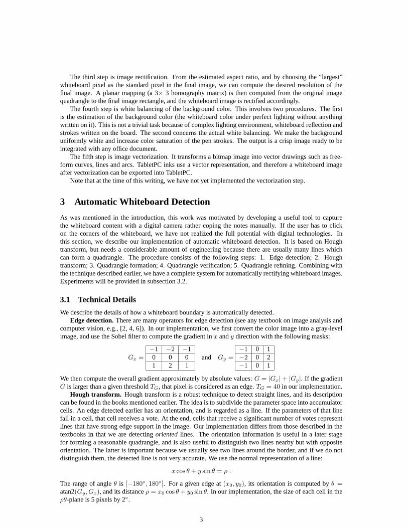
Figure 2: An example of bad quadrangles

Quadrangle verification. The lines detected from Hough space are infinite lines: they do not saywhere the supporting edges are. For example, the four lines in Figure 2 would pass all the tests described inthe previous paragraph, although the formed quadrangle is not a real one. To verify whether a quadrangle isa real one, we walk through the sides of the quadrangle and count the number of edges along the sides. Anedge within 3 pixels from a side of the quadrangle and having similar orientation is considered to belongto the quadrangle. We use the ratio of the number of supporting edges to the circumference as the qualitymeasure of a quadrangle. The quadrangle having the highest quality measure is retained as the one we arelooking for.

Quadrangle refining. The lines thus detected are not very accurate because of the discretization ofthe Hough space. To improve the accuracy, we perform line fitting for each side. For that, we first findall edges with a small neighborhood (10 pixels) and having similar orientation to the side. We then useleast-median squares to detect outliers [10], and finally we perform a least-squares fitting to the remaininggood edges [2].

3.2 Experiments With Automatic Whiteboard Rectification

We have tested the proposed technique with more than 50 images taken by different people with differentcameras in different rooms. All the tuning parameters have been fixed once for all, as we already indicatedearlier. The success rate is more than 90%. The four failures are due to poor boundary contrast, or to toonoisy edge detection. In this subsection, we provide three examples of success (Figures 3 to 5) and oneexample of failure (Figure 6).

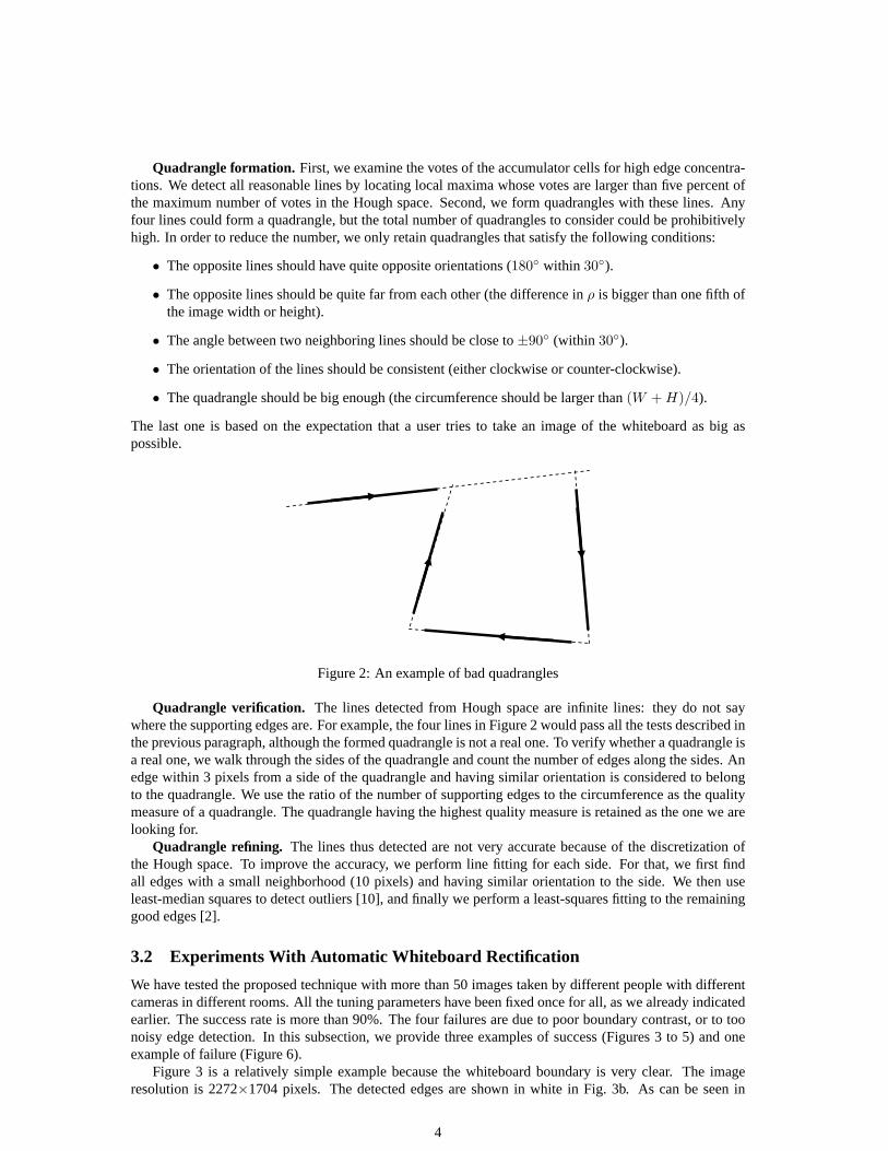
Figure 3 is a relatively simple example because the whiteboard boundary is very clear. The imageresolution is 2272×1704 pixels. The detected edges are shown in white in Fig. 3b. As can be seen in

4

(a) (b)

(c) (d)

Figure 3: Example 1. Automatic whiteboard detection and rectification: (a) Original image together withthe detected corners shown in small white squares; (b) Edge image; (c) Hough image withρ in horizontalaxis andθ in vertical axis; (d) Cropped and rectified whiteboard image.

(a) (b)

(c) (d)

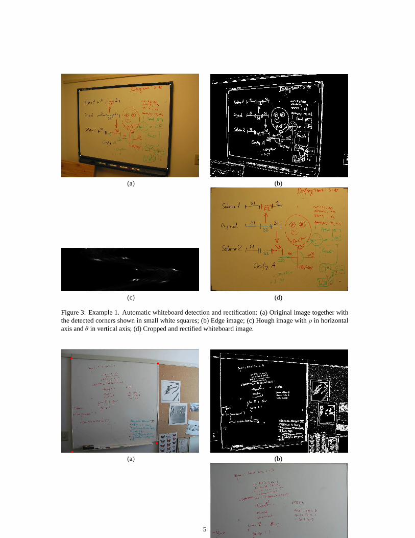
Figure 4: Example 2. Automatic whiteboard detection and rectification: (a) Original image together withthe detected corners shown in small red dots; (b) Edge image; (c) Hough image withρ in horizontal axisandθ in vertical axis; (d) Cropped and rectified whiteboard image.

5

(a) (b)

(c) (d)

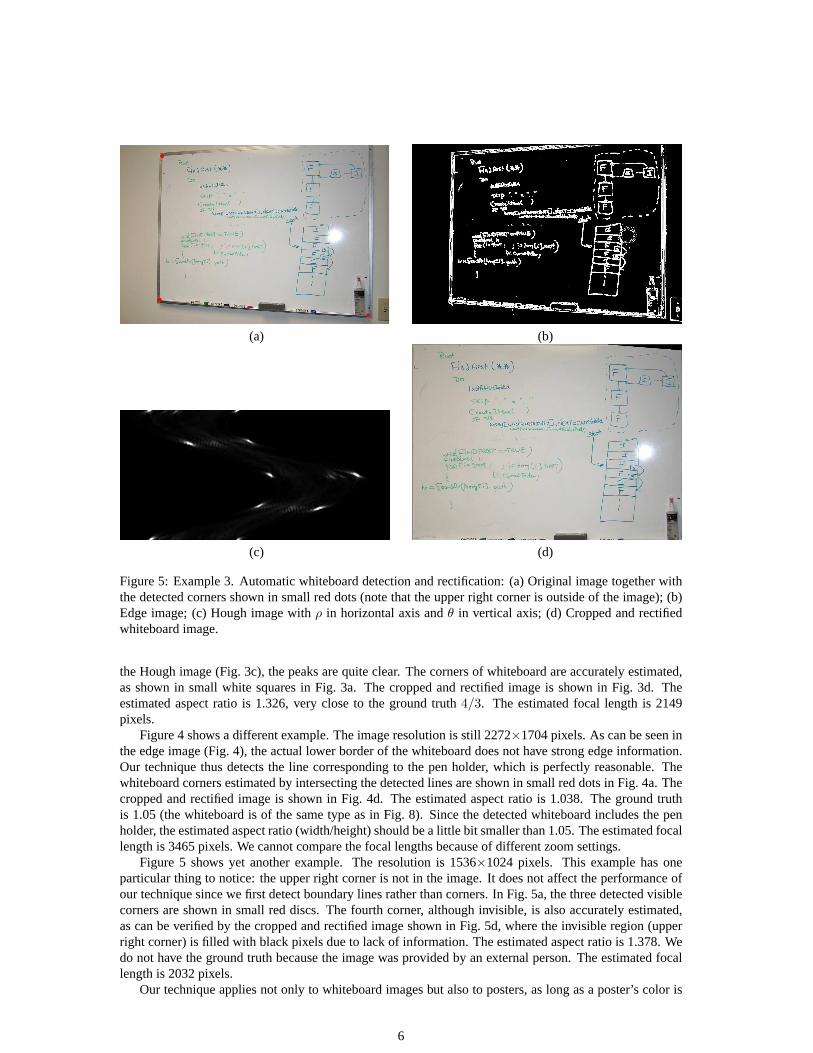
Figure 5: Example 3. Automatic whiteboard detection and rectification: (a) Original image together withthe detected corners shown in small red dots (note that the upper right corner is outside of the image); (b)Edge image; (c) Hough image withρ in horizontal axis andθ in vertical axis; (d) Cropped and rectifiedwhiteboard image.

the Hough image (Fig. 3c), the peaks are quite clear. The corners of whiteboard are accurately estimated,as shown in small white squares in Fig. 3a. The cropped and rectified image is shown in Fig. 3d. Theestimated aspect ratio is 1.326, very close to the ground truth4/3. The estimated focal length is 2149pixels.

Figure 4 shows a different example. The image resolution is still 2272×1704 pixels. As can be seen inthe edge image (Fig. 4), the actual lower border of the whiteboard does not have strong edge information.Our technique thus detects the line corresponding to the pen holder, which is perfectly reasonable. Thewhiteboard corners estimated by intersecting the detected lines are shown in small red dots in Fig. 4a. Thecropped and rectified image is shown in Fig. 4d. The estimated aspect ratio is 1.038. The ground truthis 1.05 (the whiteboard is of the same type as in Fig. 8). Since the detected whiteboard includes the penholder, the estimated aspect ratio (width/height) should be a little bit smaller than 1.05. The estimated focallength is 3465 pixels. We cannot compare the focal lengths because of different zoom settings.

Figure 5 shows yet another example. The resolution is 1536×1024 pixels. This example has oneparticular thing to notice: the upper right corner is not in the image. It does not affect the performance ofour technique since we first detect boundary lines rather than corners. In Fig. 5a, the three detected visiblecorners are shown in small red discs. The fourth corner, although invisible, is also accurately estimated,as can be verified by the cropped and rectified image shown in Fig. 5d, where the invisible region (upperright corner) is filled with black pixels due to lack of information. The estimated aspect ratio is 1.378. Wedo not have the ground truth because the image was provided by an external person. The estimated focallength is 2032 pixels.

Our technique applies not only to whiteboard images but also to posters, as long as a poster’s color is

6

(a) (b)

(c) (d)

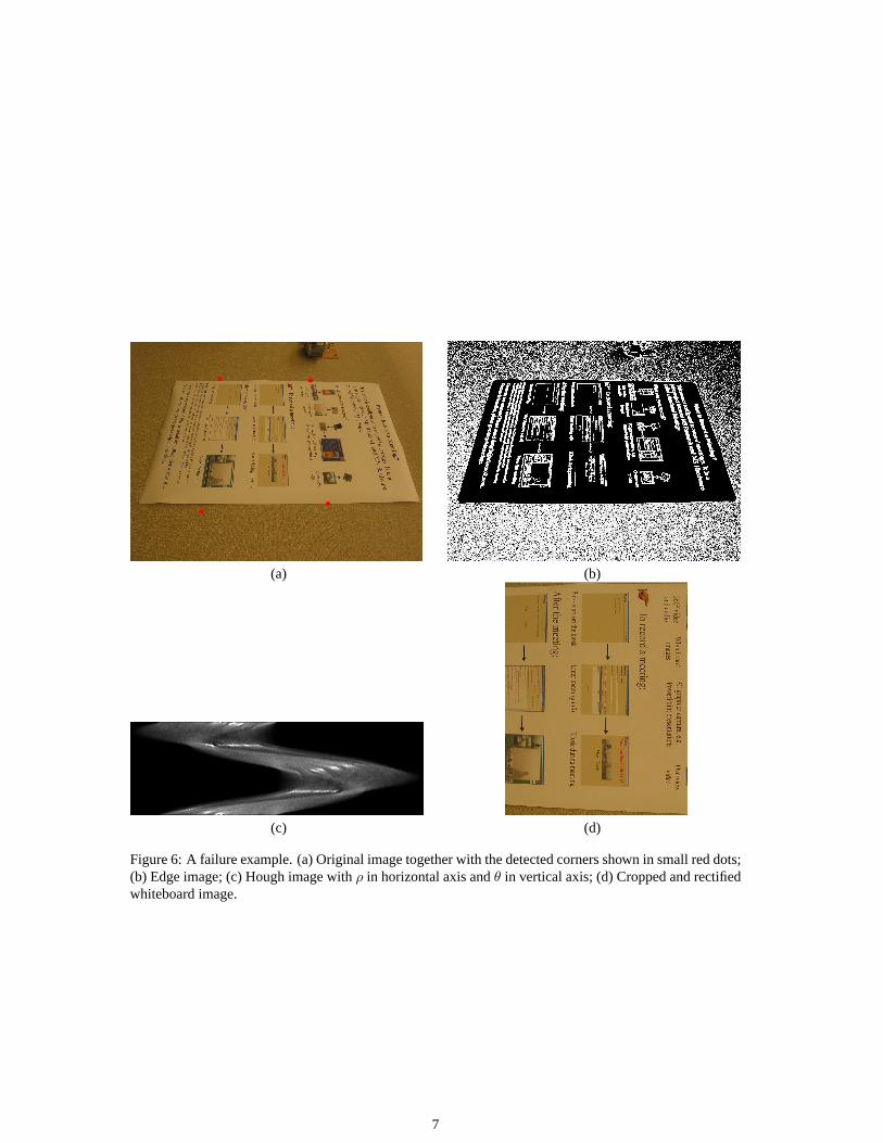
Figure 6: A failure example. (a) Original image together with the detected corners shown in small red dots;(b) Edge image; (c) Hough image withρ in horizontal axis andθ in vertical axis; (d) Cropped and rectifiedwhiteboard image.

7

distinct from the walls. Here, however, we show a failure example with a poster (Figure 6a). The failureis due to the fine texture on the wall. As can be seen in Figure 6b, the edge image is very noisy, and thenumber of edges is huge. The noise is also reflected in the Hough image (Figure 6c). The detected corners,as shown in red dots in Figure 6a, are not what we expected. For this example, we could apply a differentedge detector or change the threshold to ignore the fine texture, but our point is to check the robustness ofour technique without changing any parameters.

4 Estimating Pose and Aspect Ratio of a Rectangular Shape fromOne Image, and the Camera’s Focal Length

Because of the perspective distortion, the image of a rectangle appears to be a quadrangle. However, sincewe know that it is a rectangle in space, we are able to estimate both the camera’s focal length and therectangle’s aspect ratio.

4.1 Geometry of a Rectangle

M1

w

hz = 0

(0,0) M2

M4M3

C

m1

m2

m4m3

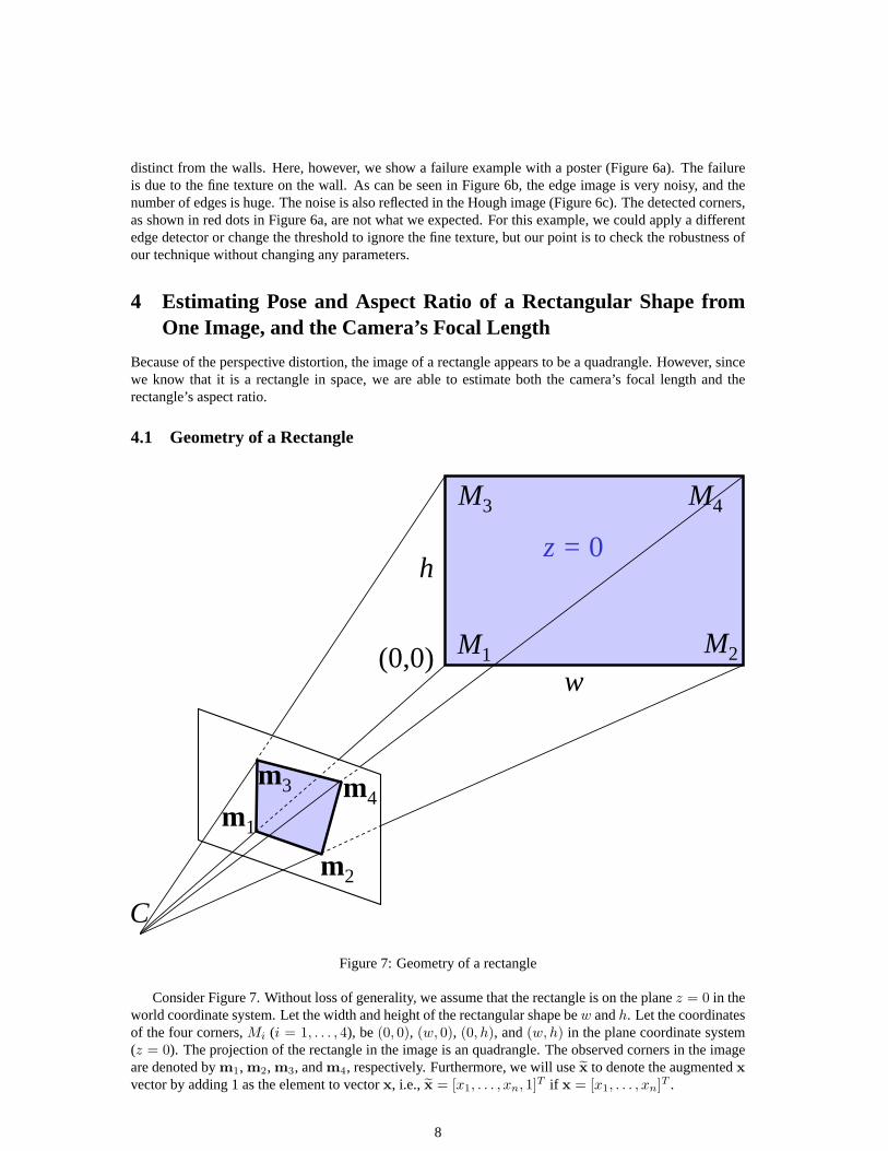
Figure 7: Geometry of a rectangle

Consider Figure 7. Without loss of generality, we assume that the rectangle is on the planez = 0 in theworld coordinate system. Let the width and height of the rectangular shape bew andh. Let the coordinatesof the four corners,Mi (i = 1, . . . , 4), be(0, 0), (w, 0), (0, h), and(w, h) in the plane coordinate system(z = 0). The projection of the rectangle in the image is an quadrangle. The observed corners in the imageare denoted bym1, m2, m3, andm4, respectively. Furthermore, we will usex to denote the augmentedxvector by adding 1 as the element to vectorx, i.e.,x = [x1, . . . , xn, 1]T if x = [x1, . . . , xn]T .

8

We use the standard pinhole model to model the projection from a space pointM to an image pointm:

λm = A[R t]M (1)

with

A =

f 0 u0

0 sf v00 0 1

and R = [r1 r2 r3]

wheref is the focal length of the camera,s is the pixel aspect ratio, and(R, t) describes the 3D transforma-tion between the world coordinate system, in which the rectangle is described, and the camera coordinatesystem. (In the above model, we assume that the pixels are not skew.) Substituting the 3D coordinates ofthe corners yields

λ1m1 = At (2)

λ2m2 = wAr1 + At (3)

λ3m3 = hAr2 + At (4)

λ4m4 = wAr1 + hAr2 + At (5)

Performing (3) - (2), (4) - (2) and (5) - (2) gives respectively

λ2m2 − λ1m1 = wAr1 (6)

λ3m3 − λ1m1 = hAr2 (7)

λ4m4 − λ1m1 = wAr1 + hAr2 (8)

Performing (8) - (6) - (7) yields

λ4m4 = λ3m3 + λ2m2 − λ1m1 (9)

Performing cross product of each side withm4 yields

0 = λ3m3 × m4 + λ2m2 × m4 − λ1m1 × m4 (10)

Performing dot product of the above equation withm3 yields

λ2(m2 × m4) · m3 = λ1(m1 × m4) · m3

i.e.,

λ2 = k2λ1 with k2 ≡ (m1 × m4) · m3

(m2 × m4) · m3(11)

Similarly, performing dot product of (10) withm2 yields

λ3 = k3λ1 with k3 ≡ (m1 × m4) · m2

(m3 × m4) · m2(12)

Substituting (11) into (6), we have

r1 = λ1w−1A−1n2 (13)

withn2 = k2m2 − m1 (14)

Similarly, substituting (12) into (7) yields

r2 = λ1h−1A−1n3 (15)

withn3 = k3m3 − m1 (16)

9

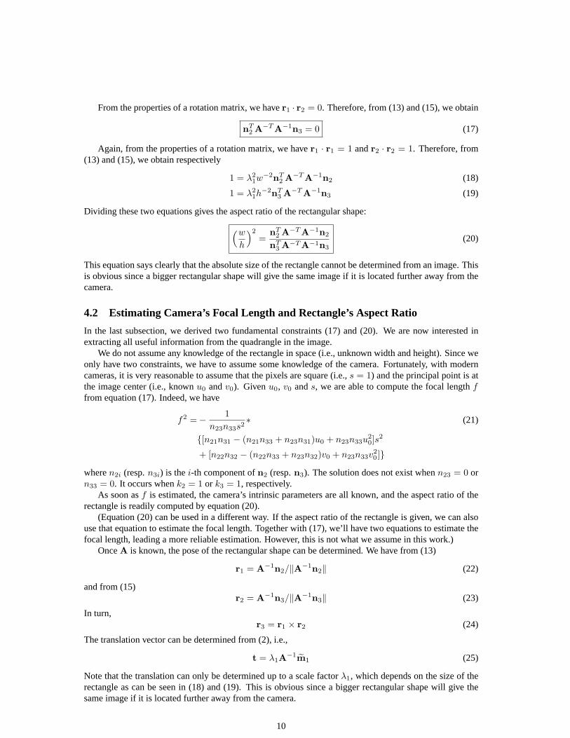
From the properties of a rotation matrix, we haver1 · r2 = 0. Therefore, from (13) and (15), we obtain

nT2 A−T A−1n3 = 0 (17)

Again, from the properties of a rotation matrix, we haver1 · r1 = 1 andr2 · r2 = 1. Therefore, from(13) and (15), we obtain respectively

1 = λ21w

−2nT2 A−T A−1n2 (18)

1 = λ21h−2nT

3 A−T A−1n3 (19)

Dividing these two equations gives the aspect ratio of the rectangular shape:

(w

h

)2

=nT

2 A−T A−1n2

nT3 A−T A−1n3

(20)

This equation says clearly that the absolute size of the rectangle cannot be determined from an image. Thisis obvious since a bigger rectangular shape will give the same image if it is located further away from thecamera.

4.2 Estimating Camera’s Focal Length and Rectangle’s Aspect Ratio

In the last subsection, we derived two fundamental constraints (17) and (20). We are now interested inextracting all useful information from the quadrangle in the image.

We do not assume any knowledge of the rectangle in space (i.e., unknown width and height). Since weonly have two constraints, we have to assume some knowledge of the camera. Fortunately, with moderncameras, it is very reasonable to assume that the pixels are square (i.e.,s = 1) and the principal point is atthe image center (i.e., knownu0 andv0). Givenu0, v0 ands, we are able to compute the focal lengthffrom equation (17). Indeed, we have

f2 =− 1n23n33s2

∗ (21)

{[n21n31 − (n21n33 + n23n31)u0 + n23n33u20]s

2

+ [n22n32 − (n22n33 + n23n32)v0 + n23n33v20 ]}

wheren2i (resp.n3i) is thei-th component ofn2 (resp.n3). The solution does not exist whenn23 = 0 orn33 = 0. It occurs whenk2 = 1 or k3 = 1, respectively.

As soon asf is estimated, the camera’s intrinsic parameters are all known, and the aspect ratio of therectangle is readily computed by equation (20).

(Equation (20) can be used in a different way. If the aspect ratio of the rectangle is given, we can alsouse that equation to estimate the focal length. Together with (17), we’ll have two equations to estimate thefocal length, leading a more reliable estimation. However, this is not what we assume in this work.)

OnceA is known, the pose of the rectangular shape can be determined. We have from (13)

r1 = A−1n2/‖A−1n2‖ (22)

and from (15)r2 = A−1n3/‖A−1n3‖ (23)

In turn,r3 = r1 × r2 (24)

The translation vector can be determined from (2), i.e.,

t = λ1A−1m1 (25)

Note that the translation can only be determined up to a scale factorλ1, which depends on the size of therectangle as can be seen in (18) and (19). This is obvious since a bigger rectangular shape will give thesame image if it is located further away from the camera.

10

(a) (b) (c)

(d) (e) (f)

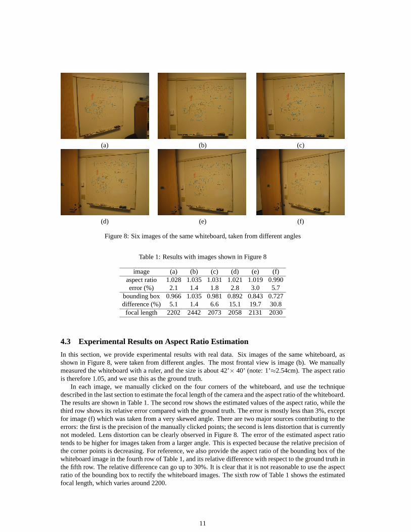
Figure 8: Six images of the same whiteboard, taken from different angles

Table 1: Results with images shown in Figure 8

image (a) (b) (c) (d) (e) (f)aspect ratio 1.028 1.035 1.031 1.021 1.019 0.990error (%) 2.1 1.4 1.8 2.8 3.0 5.7

bounding box 0.966 1.035 0.981 0.892 0.843 0.727difference (%) 5.1 1.4 6.6 15.1 19.7 30.8focal length 2202 2442 2073 2058 2131 2030

4.3 Experimental Results on Aspect Ratio Estimation

In this section, we provide experimental results with real data. Six images of the same whiteboard, asshown in Figure 8, were taken from different angles. The most frontal view is image (b). We manuallymeasured the whiteboard with a ruler, and the size is about 42’× 40’ (note: 1’≈2.54cm). The aspect ratiois therefore 1.05, and we use this as the ground truth.

In each image, we manually clicked on the four corners of the whiteboard, and use the techniquedescribed in the last section to estimate the focal length of the camera and the aspect ratio of the whiteboard.The results are shown in Table 1. The second row shows the estimated values of the aspect ratio, while thethird row shows its relative error compared with the ground truth. The error is mostly less than 3%, exceptfor image (f) which was taken from a very skewed angle. There are two major sources contributing to theerrors: the first is the precision of the manually clicked points; the second is lens distortion that is currentlynot modeled. Lens distortion can be clearly observed in Figure 8. The error of the estimated aspect ratiotends to be higher for images taken from a larger angle. This is expected because the relative precision ofthe corner points is decreasing. For reference, we also provide the aspect ratio of the bounding box of thewhiteboard image in the fourth row of Table 1, and its relative difference with respect to the ground truth inthe fifth row. The relative difference can go up to 30%. It is clear that it is not reasonable to use the aspectratio of the bounding box to rectify the whiteboard images. The sixth row of Table 1 shows the estimatedfocal length, which varies around 2200.

11

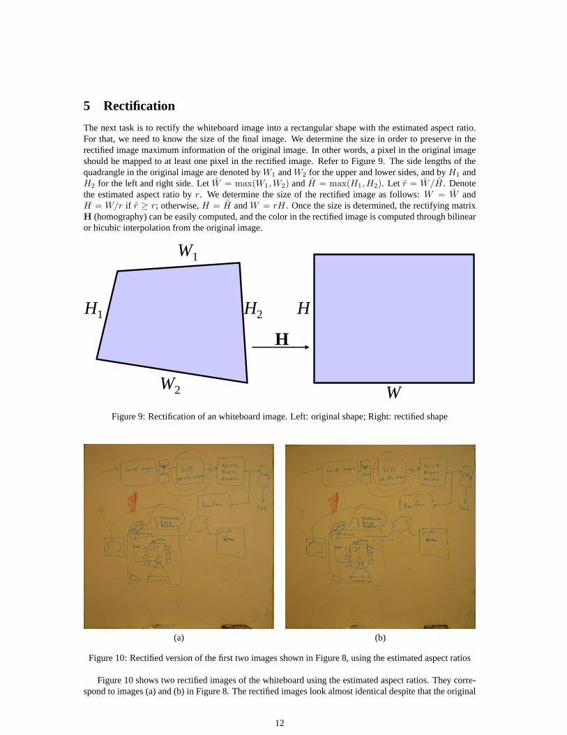
5 Rectification

The next task is to rectify the whiteboard image into a rectangular shape with the estimated aspect ratio.For that, we need to know the size of the final image. We determine the size in order to preserve in therectified image maximum information of the original image. In other words, a pixel in the original imageshould be mapped to at least one pixel in the rectified image. Refer to Figure 9. The side lengths of thequadrangle in the original image are denoted byW1 andW2 for the upper and lower sides, and byH1 andH2 for the left and right side. LetW = max(W1,W2) andH = max(H1,H2). Let r = W/H. Denotethe estimated aspect ratio byr. We determine the size of the rectified image as follows:W = W andH = W/r if r ≥ r; otherwise,H = H andW = rH. Once the size is determined, the rectifying matrixH (homography) can be easily computed, and the color in the rectified image is computed through bilinearor bicubic interpolation from the original image.

W1

W2

H1 H2

W

H

H

Figure 9: Rectification of an whiteboard image. Left: original shape; Right: rectified shape

(a) (b)

Figure 10: Rectified version of the first two images shown in Figure 8, using the estimated aspect ratios

Figure 10 shows two rectified images of the whiteboard using the estimated aspect ratios. They corre-spond to images (a) and (b) in Figure 8. The rectified images look almost identical despite that the original

12

images were taken from quite different angles. Other rectified images are also similar, and are thus notshown.

6 White Balancing

The goal of color enhancement is to transform the input whiteboard image into an image with the samepen strokes on uniform background (usually white). For each pixel, the color valueCinput captured bythe camera can be approximated by the product of the incident lightClight, the pen colorCpen, and thewhiteboard colorCwb. Since the whiteboard is physically built to be uniformly color, we can assumeCwb

is constant for all the pixels, the lack of uniformity in the input image is due to different amount of incidentlight to each pixel. Therefore, the first procedure in the color enhancement is to estimateClight for eachpixel, the result of which is in fact an image of the blank whiteboard.

Our system computes the blank whiteboard image by inferring the value of pixels covered by the strokesfrom their neighbors. Rather than computing the blank whiteboard color at the input image resolution, ourcomputation is done at a coarser level to lower the computational cost. This approach is reasonable becausethe blank whiteboard colors normally vary smoothly. The steps are as follows:

1. Divide the whiteboard region into rectangular cells. The cell size should be roughly the same as whatwe expect the size of a single character on the board (15 by 15 pixels in our implementation).

2. Sort the pixels in each cell by their luminance values. Since the ink absorbs the incident light, theluminance of the whiteboard pixels is higher than stroke pixels’. The whiteboard color within thecell is therefore the color with the highest luminance. In practice, we average the colors of the pixelsin the top 25 percentile in order to reduce the error introduced by sensor noise.

3. Filter the colors of the cells by locally fitting a plane in the RGB space. Occasionally there are cellsthat are entirely covered by pen strokes, the cell color computed in Step 2 is consequently incorrect.Those colors are rejected as outliers by the locally fitted plane and are replaced by the interpolatedvalues from its neighbors.

Once the image of the blank whiteboard is computed, the input image is color enhanced in two steps:

1. Make the background uniformly white. For each cell, the computed whiteboard color (equivalent tothe incident lightClight) is used to scale the color of each pixel in the cell:Cout = min(1, Cinput/Clight).

2. Reduce image noise and increase color saturation of the pen strokes. We remap the value of eachcolor channel of each pixel according to an S-shaped curve:0.5 − 0.5 ∗ cos(Cp

outπ). The steepnessof the S-curve is controlled byp. In our implementation,p is set to 0.75.

7 Examples

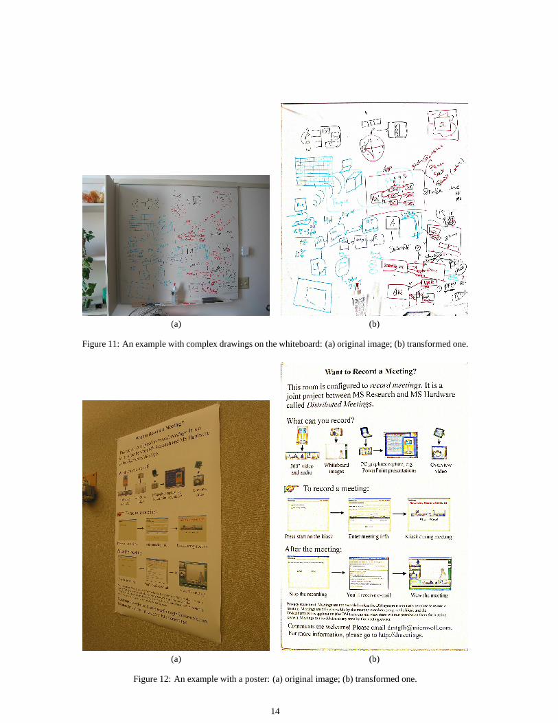
In this section, we provide a few results.Figure 11 shows our system working on whiteboard with complex drawings and complex lighting

condition.Figure 12 shows that our system also works on a poster.Figure 13 shows two images of the same whiteboard but taking from very different angles. The aspect

ratio estimated from both images is very close to the ground truth.

8 Competitive Product

The only commercial product we are aware of isWhiteboard Photo from PolyVision(http://www.websterboards.com/products/wbp.html). The list price is $249.00. Compared with our sys-tem, it lacks two features:

13

(a) (b)

Figure 11: An example with complex drawings on the whiteboard: (a) original image; (b) transformed one.

(a) (b)

Figure 12: An example with a poster: (a) original image; (b) transformed one.

14

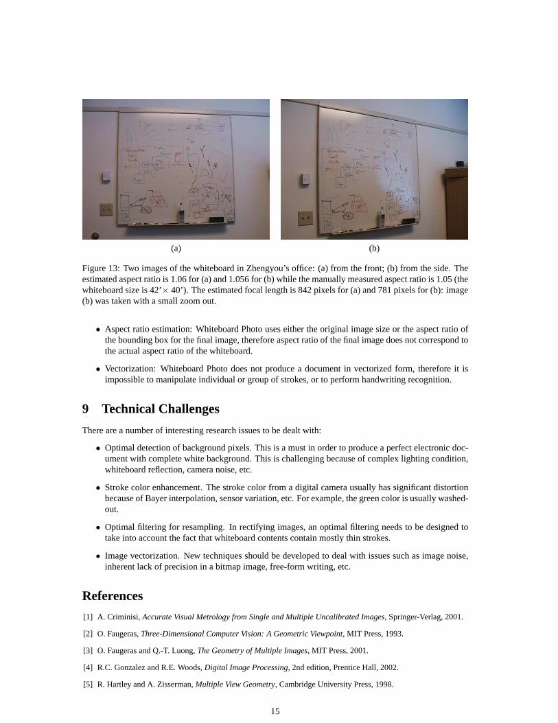
(a) (b)

Figure 13: Two images of the whiteboard in Zhengyou’s office: (a) from the front; (b) from the side. Theestimated aspect ratio is 1.06 for (a) and 1.056 for (b) while the manually measured aspect ratio is 1.05 (thewhiteboard size is 42’× 40’). The estimated focal length is 842 pixels for (a) and 781 pixels for (b): image(b) was taken with a small zoom out.

• Aspect ratio estimation: Whiteboard Photo uses either the original image size or the aspect ratio ofthe bounding box for the final image, therefore aspect ratio of the final image does not correspond tothe actual aspect ratio of the whiteboard.

• Vectorization: Whiteboard Photo does not produce a document in vectorized form, therefore it isimpossible to manipulate individual or group of strokes, or to perform handwriting recognition.

9 Technical Challenges

There are a number of interesting research issues to be dealt with:

• Optimal detection of background pixels. This is a must in order to produce a perfect electronic doc-ument with complete white background. This is challenging because of complex lighting condition,whiteboard reflection, camera noise, etc.

• Stroke color enhancement. The stroke color from a digital camera usually has significant distortionbecause of Bayer interpolation, sensor variation, etc. For example, the green color is usually washed-out.

• Optimal filtering for resampling. In rectifying images, an optimal filtering needs to be designed totake into account the fact that whiteboard contents contain mostly thin strokes.

• Image vectorization. New techniques should be developed to deal with issues such as image noise,inherent lack of precision in a bitmap image, free-form writing, etc.

References

[1] A. Criminisi, Accurate Visual Metrology from Single and Multiple Uncalibrated Images, Springer-Verlag, 2001.

[2] O. Faugeras,Three-Dimensional Computer Vision: A Geometric Viewpoint, MIT Press, 1993.

[3] O. Faugeras and Q.-T. Luong,The Geometry of Multiple Images, MIT Press, 2001.

[4] R.C. Gonzalez and R.E. Woods,Digital Image Processing, 2nd edition, Prentice Hall, 2002.

[5] R. Hartley and A. Zisserman,Multiple View Geometry, Cambridge University Press, 1998.

15

[6] R. Jain, R. Kasturi, and B.G. Schunck,Machine Vision, McGraw-Hill, Inc., 1995.

[7] K. Kanatani,Geometric Computation for Machine Vision, Oxford University Press, 1993.

[8] C. Lin and R. Nevatia, “Building Detection and Description from a Single Intensity Image”,Computer Vision andImage Understanding, 72(2):101–121,1998.

[9] PolyVision,Whiteboard Photo, http://www.websterboards.com/products/wbp.html

[10] Z. Zhang, Parameter estimation techniques: a tutorial with application to conic fitting”,Image and VisionComputing, 15(1):59–76, 1997.

16