White Paper - HSBC Global Asset Management€¦ · and timely rebalancing between a risky asset...

Target volatility strategies for insurance

companies

Rationale, benefits and pitfalls

Authored by:

Patrice Conxicoeur

CEO, Japan

Karine Desaulty

Deputy Head of Risk Managed Solutions and

Structured Products, France

White Paper February 2016

PUBLIC - For professional clients only

2

Target Volatility Strategies Executive Summary Introduction

Target volatility strategies

Historical data analysis

History sometimes doesn’t repeat itself

Random scenario analysis

Conclusion

Writers

Appendices

PUBLIC

The facts

Volatility is a well known feature of financial

markets. With major regulatory changes and low

yields everywhere, volatility has recently become

public enemy number 1 for insurers. With equities

now yielding more than treasuries in most markets,

this is unfortunate to say the least.

In this context, target volatility strategies, which

increase exposure when volatility trends down and

reduce exposure when volatility trends up, could

prove especially useful, under the assumption that

when markets are doing well volatility is low and

exposure can be high, and vice-versa, making it

worth the cost. Such strategies might thus improve

levels of return on capital as expressed through

Solvency Capital Ratios (SCR) and perhaps even

protect from downside risk.

Whether using simple or sophisticated models, all

target volatility strategies work in the same way:

they adjust exposure between a risky and a non-

risky asset depending on the level of underlying

anticipated volatility versus the target volatility. The

difference thus lies in the method chosen to supply

the anticipated volatility.

Page 3

Page 3

Page 8

Page 10

Page 11

Page 12

Page 13

Key findings

A comparison based on historical data shows that

a complex strategy – based on a GARCH model –

delivers better returns overall and better risk

control (i.e. a lower volatility of volatility) than a

historical target volatility strategy, while an

approach based on a constant mix often fails to

meet the target volatility.

Similarly, historical data shows that, over the last

18 years, a GARCH Target Volatility Strategy

(TVS) would have offered the best annualised

performance for an average SCR across

regulatory regimes (Solvency II, LAGIC and

RBC), though not always over shorter periods.

Moving away from historical performance, in a

random scenario analysis TVS also deliver lower

volatility of volatility and reduce the impact of

extreme events. However, it is difficult to conclude

whether TVS improve the Sharpe Ratio compared

with a constant mix strategy.

Overall, an investment process like volatility

targeting can serve a clear purpose if its

limitations are well understood. A major one is

that while volatility targeting can help with limiting

extreme outcomes, it cannot deliver certain

downside protection on its own: additional hedges

are needed. From a common sense as well as a

regulatory perspective, the only true capital relief

an insurer will get under the standard Solvency II

model (and others) will occur via a hedge.

To be really relevant, targeted volatility strategies

need to be associated with turbulent market

conditions. These strategies will best prove their

consistency over time in a context with periods of

high volatility.

3

Introduction

PUBLIC

Much has been written about the pro-cyclicality of

emerging insurance solvency regulations – think

Solvency II and its brethren around the globe. Their

common thread, explicitly or not, is the requirement

that insurers be demonstrably able to withstand a

“hundred-year storm”, as (however imperfectly)

encapsulated in a VaR (Value at Risk) number.

Mathematically, VaR and volatility go hand in hand. It

is thus particularly unfortunate that such solvency

regimes are coming on top of accountancy reforms

pushing for more “market consistent” (read: “marked

to market”) valuations of assets and liabilities, which

will inevitably lead to more volatility in financial results,

to the dismay of CFOs and shareholders alike. For

insurers, volatility has thus become public enemy

number one, and equities its main conduit. Pressure

has never been so great to minimise volatility, given

stakeholders’ growing intolerance of uncertainty. To

add to this perfect storm, decades-low interest rates

have robbed insurance CFOs and CIOs of any margin

of error they once enjoyed. No wonder that equity

holdings which, as a proportion of insurers’ general

accounts, stood routinely in the high teens in the

middle of the 1990s, stood barely above zero by the

end of the noughties.

In truth, insurers didn’t wait for the advent of solvency-

based regimes to reduce equity holdings: previous

crises, a bond bull market, and a few near-death

experiences post the dot-com bubble had seen to it

already. But with the bond bull market officially over,

and most equity markets now yielding more than their

reference treasuries, the lure of equities can seem

inescapable. And indeed we have seen a timid rise in

equity holdings, albeit not to pre-Global Financial

Crisis levels. In North American variable annuity

books, this has overwhelmingly taken the form of

target volatility strategies, apparently for very good

reasons. Those strategies will be the focus of this

article. We will consider how they work, what risk and

return profile they offer, what options are available to

investors, their benefits and potential pitfalls.

4

Target volatility strategies Is the theory supported by facts?

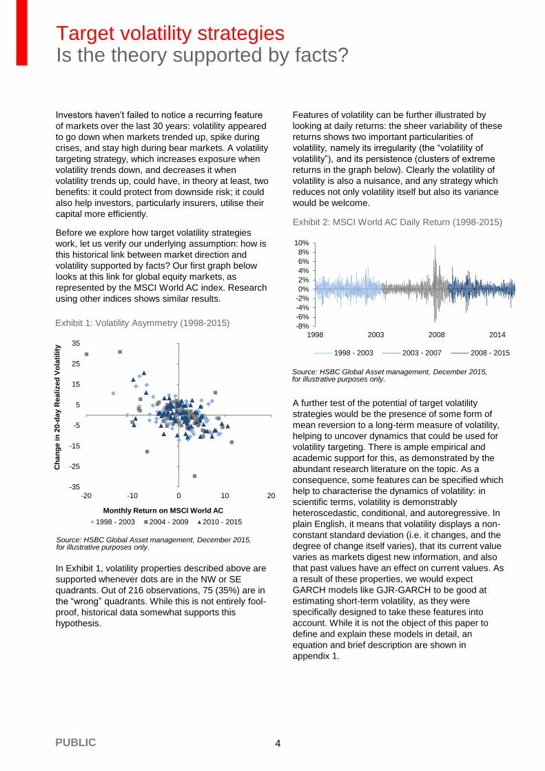
Investors haven’t failed to notice a recurring feature

of markets over the last 30 years: volatility appeared

to go down when markets trended up, spike during

crises, and stay high during bear markets. A volatility

targeting strategy, which increases exposure when

volatility trends down, and decreases it when

volatility trends up, could have, in theory at least, two

benefits: it could protect from downside risk; it could

also help investors, particularly insurers, utilise their

capital more efficiently.

Before we explore how target volatility strategies

work, let us verify our underlying assumption: how is

this historical link between market direction and

volatility supported by facts? Our first graph below

looks at this link for global equity markets, as

represented by the MSCI World AC index. Research

using other indices shows similar results.

In Exhibit 1, volatility properties described above are

supported whenever dots are in the NW or SE

quadrants. Out of 216 observations, 75 (35%) are in

the “wrong” quadrants. While this is not entirely fool-

proof, historical data somewhat supports this

hypothesis.

PUBLIC

Features of volatility can be further illustrated by

looking at daily returns: the sheer variability of these

returns shows two important particularities of

volatility, namely its irregularity (the “volatility of

volatility”), and its persistence (clusters of extreme

returns in the graph below). Clearly the volatility of

volatility is also a nuisance, and any strategy which

reduces not only volatility itself but also its variance

would be welcome.

A further test of the potential of target volatility

strategies would be the presence of some form of

mean reversion to a long-term measure of volatility,

helping to uncover dynamics that could be used for

volatility targeting. There is ample empirical and

academic support for this, as demonstrated by the

abundant research literature on the topic. As a

consequence, some features can be specified which

help to characterise the dynamics of volatility: in

scientific terms, volatility is demonstrably

heteroscedastic, conditional, and autoregressive. In

plain English, it means that volatility displays a non-

constant standard deviation (i.e. it changes, and the

degree of change itself varies), that its current value

varies as markets digest new information, and also

that past values have an effect on current values. As

a result of these properties, we would expect

GARCH models like GJR-GARCH to be good at

estimating short-term volatility, as they were

specifically designed to take these features into

account. While it is not the object of this paper to

define and explain these models in detail, an

equation and brief description are shown in

appendix 1.

Source: HSBC Global Asset management, December 2015, for illustrative purposes only.

Exhibit 1: Volatility Asymmetry (1998-2015)

Exhibit 2: MSCI World AC Daily Return (1998-2015)

Source: HSBC Global Asset management, December 2015, for illustrative purposes only.

-35

-25

-15

-5

5

15

25

35

-20 -10 0 10 20

Ch

an

ge in

20-d

ay R

eali

zed

Vo

lati

lity

Monthly Return on MSCI World AC

1998 - 2003 2004 - 2009 2010 - 2015

-8%

-6%

-4%

-2%

0%

2%

4%

6%

8%

10%

1998 2003 2008 2014

1998 - 2003 2003 - 2007 2008 - 2015

5

Target volatility strategies Historical data: testing different models

PUBLIC

The next step leads us to look at the practical

aspects of a target volatility strategy. What volatility

are we talking about: backward looking, or forward

looking using some kind of predictive model? As

shown above, the temptation is strong to use a

sophisticated approach, namely a GJR-GARCH

model, but what about using something simpler like a

constant mix or a simple reference to a long-term

average? Most importantly, what return profiles

should investors expect? In this section we will

attempt to shed some light on those crucial

questions.

Simplistically, a review of the available literature on

the topic reveals there are two sides to the debate.

The first, presumably populated by providers of

target volatility products, is extremely supportive of

them. More sceptical, the second highlights the risks

associated with such strategies, namely model risks,

gaps risks, and risks of volatility not behaving as

expected e.g. being low on the upside / high on the

downside.1

Nonetheless, all target volatility strategies rely on a

similar approach, with the aim of targeting the

desired level of volatility by performing appropriate

and timely rebalancing between a risky asset (e.g.

index futures) and a non-risky asset (e.g. cash or T-

bills). The process is simple and transparent:

whether using a sophisticated GARCH approach or a

simple “moving average” design, the strategies

adjust their exposure depending on the level of

underlying anticipated volatility vs. the target

volatility. When expected market volatility is higher

than the target volatility, exposure is reduced and

vice versa. The target equity exposure to risky assets

can be determined daily by dividing the targeted

volatility by the anticipated volatility. Interestingly, this

potentially opens the way to a leveraged exposure

when anticipated volatility is lower than the target

volatility – something which will not be palatable to all

investors. We will look at an unleveraged approach

below, and show results for a leveraged approach in

Appendix 2.

The difference between various strategies therefore

lies in the method chosen to supply the anticipated

volatility, two of which we will analyse in the

examples below. In the first case, which we called

“Historical Target Volatility Strategy” or HTVS, the

anticipated volatility is calculated as the standard

deviation of the last 20 daily index returns. In the

second case, “GARCH Target Volatility Strategy” or

GTVS for short, the anticipated volatility is computed

with a GJR-GARCH model calibrated on the

underlying index.

As shown below, we tested both approaches with

target volatility strategies invested on the MSCI

World Total Return with net dividend reinvested

(hedged in USD)2. In parallel with these two target

volatility strategies and in order to compare them with

a simpler approach, we included a “constant mix”

strategy (CMS) in the examples.

Key assumptions:

Currency = USD

Non-risky asset = US T-bills 3 months

Exposure threshold: To minimise transaction

costs, the exposure is modified if the difference

between the exposure of the strategy and the

target exposure is higher than a threshold, which

we put at 5%

The GARCH GJR model is calibrated over ten

years and re-estimated each year for use in the

following year, so as not to have an “in sample”

bias. Hence tests below start in early 1998.

The historical volatility is calculated over a 20-day

period.

Index data are re-calculated between 31/12/87

and 31/12/01, then sourced from Bloomberg.

Target Volatility: 10%

Terminology:

GTVS is the strategy with the GARCH model

HTVS is the strategy with historical volatility

CMS is a constant mix strategy

- CMS is designed to also have a constant level

of exposure but this level is calculated from the

long term volatility of the market (here 14%)

and the target volatility (here 10%).

The strategies’ realised volatility is calculated as

the annualised standard deviation of daily returns,

while the volatility of volatility is calculated as the

standard deviation of the 20-day volatility.

1 Interestingly, no author seems to have taken an interest in the intricacies of implementing such a strategy from a fiduciary perspective, with the associated requirements in terms of transparency, best execution and duty of utmost care. We’ll leave this aside for another discussion, but suffice to say at this stage that those things matter, cannot be taken for granted, and need to be addressed. 2 While the use of currency hedged returns may seem slightly incongruous for equity strategies, this in fact anticipates the implementation of the strategies with index futures for cost and liquidity reasons: index futures deliver pure equity returns and very little currency exposure.

6 PUBLIC

Exhibit 3: Representative portfolios’ outperformance - % versus their respective initial allocation - (1998-2015)

Source: HSBC Global Asset Management, December 2015. Past performance and back tested (simulated) data are not a reliable indicator of future returns.

Exhibit 4: Performance (1998-2015)


Exhibit 5: Exposures (1998-2015)


Index GARCH Target

Volatility (GTVS)

Historical Volatility

(HTVS) CMS Target Vol

Target volatility - 10% 10% 10%

Realised volatility 15.9% 9.6% 10.0% 11.3%

Volatility of volatility 7.8% 2.0% 2.5% 5.6%

Max Drawdown -54% -39% -43% -42%

Annualised performance 5.21% 5.68% 4.68% 4.58%

Strategy average exposure 100% 78% 78% 71%

GTVS

Index

HTVS

CMS

80

120

160

200

240

280

12/1997 12/1999 12/2001 12/2003 12/2005 12/2007 12/2009 12/2011 12/2013 12/2015

0%

10%

20%

30%

40%

50%

60%

70%

80%

90%

100%

12/1997 12/1999 12/2001 12/2003 12/2005 12/2007 12/2009 12/2011 12/2013 12/2015

GTVS

HTVS CMS

7 PUBLIC

Exhibit 6: Realised 20-day Volatility (1998-2015)


The volatility graphs above shows that GTVS

delivers better risk control, as its realised 20-day

volatility hugs the 10% target much more closely

than other approaches. From this perspective, the

approach based on a constant mix is a failure: it is

entirely swayed by the index, and often very far

from the objective.

0%

10%

20%

30%

40%

50%

60%

70%

1998 2000 2002 2004 2006 2008 2010 2012 2014

Index HTVS GTVS CMS Target Volatility: 10%

8

Annual returns as shown above demonstrate that

overall GTVS offers more satisfying results than

other approaches, even if it is not entirely fool-proof

(e.g. in 2000). Predictably, all approaches lag the

index whenever it shoots up, such as in 2009 or

2013.

PUBLIC

Exhibit 7: Annual performances


Clearly, GTVS and HTVS can deliver the

predetermined volatility target. GTVS yields the best

results, thanks to a lower volatility of volatility, and

perhaps most importantly a reduction in extreme

losses (as shown above with the distribution of

quarterly returns) which helps to deliver, in this

example at least, better returns overall, and with

fewer scares along the way. This is strongly

confirmed by 95% 1-year VaR and 1-year CVar as

shown below.

Predictably, the results of our own research fall

somewhere in between the two sides mentioned

earlier. Sophisticated target volatility strategies seem

to perform mostly as advertised when it comes to

controlling volatility, but remain vulnerable to jumps

and gaps in the market, and will suffer if the markets

trend down with little or no volatility. An additional

insight gained here is that sophistication seems to

pay: simple approaches either fail or deliver the

target less smoothly. Lastly and importantly, this

simulation also shows that the downside protection is

limited with all strategies, even if the GARCH

approach appears to do a better job in this area3.

Exhibit 8: Distribution of quarterly performances


Exhibit 9: 95%VaR and cVaR over 1 year

Source: HSBC Global Asset Management, December 2015. For illustrative purpose only.

3 Perhaps importantly for investors who had in the past invested in what were then poorly designed forward guaranteed products, some of which ended up being liquidated, target volatility strategies do not cash out: they do not turn into a money market fund where equity exposure was intended.

Index

Volatility Index GTVS HTVS CMS

1998 16.5 21.5 20.9 15.2 16.9

1999 12.4 29.1 24.7 23.1 21.8

2000 15.7 -8.4 -9.3 -7.7 -4.3

2001 16.9 -14.0 -11.6 -16.8 -9.0

2002 21.6 -24.7 -17.6 -17.2 -17.6

2003 14.6 24.4 17.3 18.0 17.5

2004 8.9 11.0 9.2 9.2 8.3

2005 7.5 16.1 16.0 15.9 12.3

2006 9.3 16.9 17.7 16.5 13.4

2007 12.7 5.6 7.1 4.5 5.5

2008 31.4 -38.4 -17.0 -19.5 -28.3

2009 21.0 26.3 11.1 11.2 18.7

2010 14.8 10.5 10.6 9.8 7.6

2011 19.0 -5.5 -4.4 -4.4 -3.6

2012 11.2 15.8 12.3 12.4 11.2

2013 9.5 28.7 25.4 25.0 19.9

2014 9.5 9.7 7.0 5.8 7.0

2015 13.7 2.0 -1.3 -0.3 1.6

Index GTVS HTVS CMS

95% 1-year VaR - strategy -27.8% -16.8% -18.9% -19.9%

95% 1-year cVaR - strategy -35.6% -18.7% -21.0% -26.0%

0%

2%

4%

6%

8%

10%

12%

14%

16%

18%

20%

-20% -16% -12% -8% -4% 0% 4% 8% 12% 16% 20%

Index GTVS HTVS CMS

9

Historical data analysis Applicability for insurers

With these results in mind, let us return to the case of

insurers, in particular those who have to worry about

cost of capital in a solvency-based framework, such

as Solvency II. The benefits outlined above are quite

clear, particularly when thinking about solvency

regimes which focus on VaR outcomes, but can this

be taken further?

It is worth remembering that in most solvency

regimes, whatever the strategy employed, it doesn’t

have a significant impact on the calculation of capital

costs. For instance, under Solvency II (standard

model), the base equity capital shock is either 39%

for OECD / EEA equities or 49% for others. Whether

the investment manager has a value, growth, active,

small cap or passive bias, the cost is the same.

Under Solvency II the only variation allowed is linked

to the “symmetric adjustment”, which bears no

relation to the underlying strategy, but rather to the

position of the market relative to its own moving

average. The objective here is to introduce a dose of

counter-cyclicality in the capital cost.

To answer a similar concern, with LAGIC4 the

Australian regulator introduced a different adjustment

mechanism, based on the variation of the dividend

yield.

In contrast, the US RBC5 doesn’t include any such

adjustment. So, what do results look like, in terms of

Solvency Capital Requirements (SCR), for those

three regimes?

Exhibit 10 shows that, over the last 18 years, GTVS

has offered the best annualised performance /

average SCR, seemingly across regulatory regimes.

However, while this is the case over the long run, it is

not always true over shorter periods.

Additionally, and while capital cost is not

differentiated by equity strategy, this only applies to

actual exposure under the look-through principle. In

other words, if volatility is low, exposure will be high,

and corresponding capital charges as well, but

markets will presumably be doing well, making it

worth the cost for insurers. Conversely, if volatility is

high, exposure will be low, while markets will

presumably not be doing well. This should be

another attractive feature for insurers, albeit not over

all periods. Appendix 2 (page 16) explores examples

using HTVS and GTVS strategies allowing leverage,

and shows similar results over the past 18 years.

4 LAGIC stands for Life and General Insurance Capital Standards and was introduced in late 2012.

5 RBC = Risk Based Capital

Period No leverage allowed Index GTVS HTVS CMS

Jan 1998 - Dec 2015 Annualised performance 5.2% 5.7% 4.7% 4.6%

Solvency II SCR (average) 39.5% 31.1% 31.2% 28.2%

Max 49.0% 49.0% 49.0% 35.0%

Min 29.0% 5.1% 5.6% 20.7%

Annualised performance / Avg SCR 13.2% 18.3% 15.0% 16.2%

Jan 1998 - Dec 2002 Annualised performance -1.4% -0.1% -2.1% 0.4%


Max 49.0% 49.0% 49.0% 35.0%

Min 29.3% 7.7% 7.8% 20.9%

Annualised performance / Avg SCR -3.3% -0.3% -6.6% 1.4%



Max 49.0% 49.0% 49.0% 35.0%

Min 29.0% 5.1% 5.6% 20.7%




Max 44.1% 44.1% 44.1% 31.5%

Min 29.0% 8.1% 7.5% 20.7%


Exhibit 10a: Solvency II impact on performance


Period No leverage allowed Index GTVS HTVS CMS

Jan 1998 - Dec 2015 Solvency II 13.2% 18.3% 15.0% 16.2%

LAGIC 13.7% 19.0% 15.6% 16.9%

RBC 21.7% 30.3% 24.9% 26.7%

Exhibit 10b: Annualised performance / average capital requirement

PUBLIC

10

History sometimes doesn’t repeat itself Random scenario analysis

The good result obtained by target volatility strategies

over the last 18 years are not the result of cherry

picking. Nevertheless, ‘past performance is not a

reliable indicator of future results’, and results might

have been very different in another market

configuration. This led us to test the robustness of the

strategy with additional scenario analyses. To proceed,

we applied a Monte Carlo method to generate a

sufficiently high number of scenarios (around 10,000

possibilities) for the risky asset. The strategies were

simulated using a non-constant volatility for the risky

asset and run against two scenarios for the sake of

avoiding biases in favour of any one strategy: one with

a Constant Risk Premium (CRP) and the other with a

Constant Sharpe Ratio (CSR).

In the example below, we compare a TVS with a

Constant Mix Strategy (CMS), which has a constant

level of exposure over time. To use a real-world

example, both are invested in the DJ Eurostoxx 50 TR

(risky asset) and in cash (risk-free asset). Since its

volatility is higher than global volatility, both strategies

target a predefined level of volatility of 12%. Given the

long-term volatility of the market (25%), the CMS’

constant level of exposure is fixed at 48% at launch –

with a 6% constant premium for equities - to target the

predefined level of volatility (12%)6.

As shown in Exhibit 11, realised volatility is close to the

pre-defined target for both the TVS and CMS.

However, under both scenarios (CRP and CSR), the

TVS enables a clear reduction of the volatility of

volatility compared to the CMS (close to 45%). The

TVS’s realised volatility exhibits a lower dispersion

around the target volatility with a reduced probability of

significant deviations from the target, as shown in the

distribution of one-year volatilities in the case of CRP

simulations in Exhibit 12 (results are similar for CSR).

The TVS thus reduces the impact of extreme events

on the left side of return distribution compared to the

CMS, with VaR and CVaR clearly reduced in both the

CRP and CSR simulations (Exhibit 13). Indeed, the

TVS reduces the equity exposure in high volatility

regimes, where extreme events are more important.

As can be seen in Exhibit 14, the TVS clearly improves

the Sharpe Ratio compared to the CMS in the CRP

simulations, but only slightly in the CSR simulations.

The assumption of the level of correlation between the

market’s prospective Sharpe Ratio and the expected

volatility is therefore key to explaining the simulation

results on the TVS Sharpe Ratio.

In practice, however, it is not easy to predict this

correlation, as both negative and positive correlations

can be found in the historical samples, making it

difficult to draw any firm conclusions as to whether the

TVS improves the Sharpe Ratio versus the CMS.

CMS TVS Volatility of

volatility reduction

CRP Average volatility 11.6% 12.5%

Volatility of volatility 4.1% 2.3% -44%

CSR Average volatility 11.6% 11.8%

Volatility of volatility 4.1% 2.2% -47%

Exhibit 11: TVS offers an efficient Volatility Control


Index CMS TVS

CRP VaR 99.5% 1 year -70.7% -41.8% -25.7%

CVaR 99.5% 1 year -84.1% -57.3% -28.6%

CSR VaR 99.5% 1 year -68.2% -39.6% -23.8%

CVaR 99.5% 1 year -82.1% -54.9% -26.8%

Exhibit 13: Extreme events

Exhibit 14: Sharpe ratios


CMS TVS

CRP - Sharpe ratio 0.25 0.32

CSR - Sharpe ratio 0.25 0.27

Exhibit 12: distribution of one-year volatilities


PUBLIC

6 Assumptions: Target Volatility : 12%; Underlying asset: Eurostoxx50; Long term volatility : 25%; Currency: EURO; Non risky asset: 0%; Constant Premium for equities : 6% (for Constant Premium Simulations); Constant Sharpe Ratio : 0.27 (for Constant Sharpe Simulations); The weights of the risky-asset and risk-free asset in the strategy are always positive and below 100%; Exposure of CMS: 48%; The strategies are managed every day on closing prices; One-year simulations; 10 000 paths

0%

20%

40%

60%

80%

> 6

%

10%

/ 12%

16%

/ 18%

22%

/ 24%

28%

/ 30%

34%

/ 36%

40%

/ 42%

46%

/ 48%

52%

/ 54%

58%

/ 60%

64%

/ 66%

Index CMS TVS

11

Random scenario analysis Applicability for insurers

Let us now analyse the results of these simulations

with a Solvency II point of view. Any strategy with a

maximum exposure of 100% and an average

exposure below 100% achieves a lower SCR than

plain equities on average. Such is the case for both

strategies with a target volatility of 12%, which is

below the long-term volatility of the market. Therefore

both the TVS and CMS achieve a lower SCR than

the index. However, as TVS’s average equity

exposure is higher than for the CMS, the GTVS

generates a higher SCR than the CMS. In terms of

return on SCR and measured in our simulations as

the average annual expected return divided by the

average SCR, Returns on SCR are similar for the

index, CMS and GTVS. The lower SCR is

compensated by a lower average expected return.

As insurers only get capital relief by hedging, we

completed our previous simulations by implementing

a downside protection – a one-year put option

offering a 90% capital protection. The goal was to

assess the practical impact of this strategy in random

market configurations – still using around 10,000

scenarios for the risky asset.

To proceed, we defined two downside protection

strategies7:

The first, DPSI, invests in the index, in a vanilla

put on the index (priced at 5.35%, implied volatility

of 25.2%) and in cash

The second, DPTVS, invests in a 12% TVS, in a

put on the TVS (priced at 1.90%) and in cash

On average, the Return on SCR is higher for the

DPSI than for the DPTVS, and both are higher than

for the index. In the simulations1, the DPSI shows a

higher average return than the DPTVS. By

construction, as the protection is set at a 90% level,

the SCR of both downside strategies is equal to 10%

(counterparty risk put aside) and the average Return

on SCR is higher for the DPSI than for the DPTVS

(Exhibit 15).

PUBLIC

Exhibit 16 shows the impact of the price of a vanilla

put on the DPSI’s average Return on SCR, to be

compared with that of the DPTVS, the TVS and the

index.

The price of the vanilla put is highly dependent on

market conditions and particularly on implied

volatility. In turn, the DPSI’s Return on SCR depends

on the price of the vanilla put, in that a higher price of

vanilla put induces a lower average Return on SCR

for the DPSI.

We will assume here that the price of the put on the

TVS does not depend on implied volatility. Therefore,

the average Return on SCR for the DPTVS, as well

as for the TVS and the index, are assumed to be

constant in the graph.

The use of a put option in the DPTVS improves its

average Return on SCR compared to that of the TVS

or the index. Exhibit 16 illustrates that the implied

volatility on the vanilla put must reach quite a high

threshold before the average Return on SCR

becomes lower for the DPSI than for the DPTVS -

The threshold corresponds to 27.5% implied volatility

for the put. The DPTVS achieves a steady average

Return on SCR over time. The most interesting

aspect of puts on the TVS is that their prices are

almost insensitive to equity volatility. Therefore, the

DPTVS reduces the uncertainty of the protection’s

rolling cost over time.


Exhibit 16: Return on SCR in function of 90% vanilla

put’s price (CRP)

Exhibit 15: Average return on SCR

0%

20%

40%

60%

3% 4% 5% 6% 7% 8% 9% 10%

Retu

rn o

n S

CR

Vanilla put price

Index TVS

DPSI DPSTV

7 Prices as of 31/12/2015

Index DPSI DPTVS

SCR 39.0% 10.0% 10.0%

CRP – Return/SCR 15.7% 31.0% 24.6%

CSR – Return/SCR 15.3% 28.3% 17.0%


DPTVS

12

Random scenario analysis Applicability for insurers

In this simulation, compared to the CMS, the TVS

is more efficient in terms of volatility control, and

to reduce the impact of extreme events. Results

are less straightforward for risk-adjusted returns

and strongly depend on assumptions around the

risky assets. In the context of insurance

regulation, one cannot conclusively credit either

the TVS or the CMS with Return on SCR

optimisation benefits, even if the average SCR is

reduced for both strategies – thanks to their

below 100% equity exposure.

Adding downside protection to the TVS and to

the index further reduces the SCR, and in most

market conditions (except for high implied

volatility in the case of the DPSI) improves the

average return on SCR. Nonetheless, according

to our simulations, average returns on SCR are

most often higher with the DPSI than with the

DPTVS, depending on the level of implied

volatility.

Overall, the most interesting aspect of the DPTVS

is its consistency over time.

PUBLIC

13

Conclusion Clear benefits with some limitations

A target volatility strategy can make a lot of sense for

many investors, particularly where capital is scarce

and must be allocated efficiently, and especially if the

rules turn volatility into public enemy number one.

This is certainly the case for insurers nowadays. In a

formulaic world, when it comes to reporting and

capital requirements, the outcome of a sophisticated

target volatility strategy is certainly desirable and can

reap substantial benefits versus a naïve approach.

There are however circumstances where the strategy

will not live up to expectations. Those include

instances where market declines occur with low

volatility. Furthermore, as with any dynamic strategy,

instances of market gaps are particularly scary, as

they do not allow for any adjustment of the exposure

to deliver the desired outcome. In an extreme case,

markets could crash and volatility spike before

exposure could practically be adjusted. Although

such occurrences have been rare in recent memory,

no one can say with certainty that this will be the

case in the future, especially in a world rife with

geopolitical uncertainties and sources of economic or

financial fragility.

Overall, an investment process like volatility targeting

can serve a clear purpose if its limitations are well

understood. A major one is that while volatility

targeting can help with limiting extreme outcomes, it

cannot deliver certain downside protection on its

own: additional hedges are needed. From a common

sense as well as a regulatory perspective, the only

true capital relief an insurer will get under the

standard Solvency II model (and others) will occur

via a hedge. In simple terms, any provider of capital

protection is short a put or a series of puts. This is

true of most insurers selling variable insurance or

variable annuity products. Like all sellers of

protection, they are at risk of facing unlimited

liabilities, with potentially ever rising capital costs, as

volatility rises and markets sink.

PUBLIC

Therefore and periodically at least, insurers must

hedge this risk, either with a dynamic hedging

strategy, or by purchasing puts to cover their short

position. This in turn creates additional risks,

particularly basis risks, such as the risk that existing

exposures are not perfectly matched by the hedges.

Target volatility products can help with both issues:

first of all, if volatility of the investment is known and

capped in advance, then the cost of the target

volatility index option8 needed to hedge the

corresponding guarantees is cheaper (target volatility

strategies aim at a lower volatility than market

volatility) and, by and large, known in advance.

Furthermore, since target volatility strategies are

typically implemented with index futures, using target

volatility index options to hedge the exposure will

essentially suffice to eliminate the basic risk. Of

course, the paradox is that if certainty of outcomes is

absolutely needed, then more capital will be required

to pay for guarantees and related options.

When combined with hedging techniques,

targeted volatility strategies improve the average

return on SCR but, typically, no more than a

simple ‘index + put’ strategy. To be really

relevant, targeted volatility strategies need to be

associated with turbulent market conditions.

These strategies will best prove their consistency

over time in a context with periods of high

volatility.

This consistency, and the ability of targeted

volatility strategies to reduce the fluctuation of

the protection’s rolling cost over time are the

main advantages to consider for insurers, who

are by nature long term investors, and who may

not have the flexibility to adjust or to review their

equity allocation at each market event.

8 A target volatility index option is an option where the underlying is a Volatility Target Strategy. The difference with a vanilla option is at the level of the underlying which is not an equity index but a Volatility Target Strategy.

14

Writer ?

Patrice Conxicoeur has been CEO, HSBC Global

Asset Management (Japan) K.K. , since 1st April,

2015. Prior to this, he was Global Head of Insurance

Coverage from May 2011, with global responsibility

for the product strategy and business development

with insurance companies, and he was Head of

Institutional Business for Asia Pacific from 2008.

Before joining HSBC, Mr Conxicoeur held a variety of

roles with Sinopia Asset Management from 1992,

moving to Asia in 2000, first in Japan as CEO of

Sinopia T&D Asset Management Co, Ltd., and from

2004 in Hong Kong as Chief Executive of Sinopia,

Asia-Pacific. From 1990 to 1992, Mr Conxicoeur

worked in Tokyo with Japan Gamma Asset

Management, after graduating from the Lyon

Graduate School of Business (now E.M. Lyon) in

1990 in France.

Patrice Conxicoeur

CEO, Japan

HSBC Global asset Management

Karine Desaulty is Deputy Head of Risk Managed

Solutions & Structured Products. She has been

working in the industry since 1997, when she joined

HSBC. Prior to her current position, Ms Desaulty

worked as a Trader and then as a Quantitative

Portfolio Manager specialising in Principal

Guaranteed and Structured Product. She holds a

Postgraduate degree from the ESSEC business

school (France) and a Postgraduate degree in

Statistics applied to Economics and Finance from

Université Paris VII (France).

Karine Desaulty

Deputy Head of Risk Managed

Solutions and Products

HSBC Global Asset Management

France

PUBLIC

15

Appendix 1 Definitions and references ?

PUBLIC

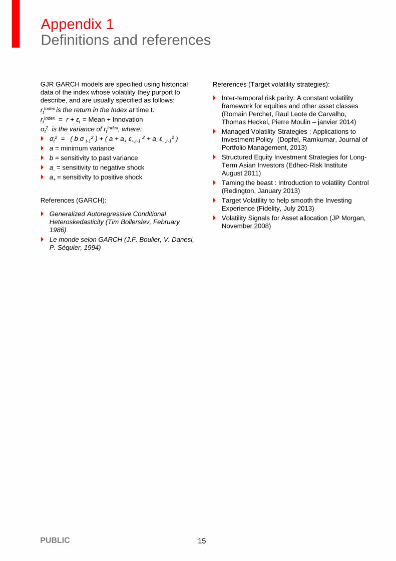
GJR GARCH models are specified using historical

data of the index whose volatility they purport to

describe, and are usually specified as follows:

rtIndex is the return in the Index at time t.

rtIndex = r + εt = Mean + Innovation

σt2 is the variance of rt

Index, where:

σt2 = ( b σ t-1

2 ) + ( a + a+ ε+,t-1 2 + a- ε- ,t-1

2 )

a = minimum variance

b = sensitivity to past variance

a- = sensitivity to negative shock

a+ = sensitivity to positive shock

References (GARCH):

Generalized Autoregressive Conditional

Heteroskedasticity (Tim Bollerslev, February

1986)

Le monde selon GARCH (J.F. Boulier, V. Danesi,

P. Séquier, 1994)

References (Target volatility strategies):

Inter-temporal risk parity: A constant volatility

framework for equities and other asset classes

(Romain Perchet, Raul Leote de Carvalho,

Thomas Heckel, Pierre Moulin – janvier 2014)

Managed Volatility Strategies : Applications to

Investment Policy (Dopfel, Ramkumar, Journal of

Portfolio Management, 2013)

Structured Equity Investment Strategies for Long-

Term Asian Investors (Edhec-Risk Institute

August 2011)

Taming the beast : Introduction to volatility Control

(Redington, January 2013)

Target Volatility to help smooth the Investing

Experience (Fidelity, July 2013)

Volatility Signals for Asset allocation (JP Morgan,

November 2008)

16

Appendix 2 Results with leverage

PUBLIC

Assumptions


Representative portfolios’ outperformance - % versus their respective initial allocation - (1998-2015)

Performance (1998-2015)

Exposures (1998-2015)

Index

GARCH Target

Volatility Strategy

(GTVS)

Historical Volatility

Strategy (HTVS)

CM Target

Vol (CMS)

Target volatility - 10% 10% 10%

Realised volatility 15.9% 10.2% 11.0% 11.3%

Volatility of volatility 7.8% 1.9% 2.5% 5.6%

Max Drawdown -54% -39% -44% -42%

Annualised performance 5.21% 5.82% 4.96% 4.58%

Average exposure 100% 84% 90% 71%

Maximum exposure 200%

Exposure threshold 5%

Volatility target 10%

GTVS

HTVS

CMS

Index

80

120

160

200

240

280

320

12/1997 12/1999 12/2001 12/2003 12/2005 12/2007 12/2009 12/2011 12/2013 12/2015

GTVS

HTVS

CMS

0%

20%

40%

60%

80%

100%

120%

140%

160%

180%

200%

12//1997 12//1999 12//2001 12//2003 12//2005 12//2007 12//2009 12//2011 12//2013 12//2015

17 PUBLIC

Realised 20-day Volatility (1998-2015)

Annual performances

Index Volatility Index GTVS HTVS CMS

1998 16.5% 21.5% 20.7% 14.9% 16.9%

1999 12.4% 29.1% 24.3% 21.9% 21.8%

2000 15.7% -8.4% -10.3% -9.2% -4.3%

2001 16.9% -14.0% -11.7% -17.0% -9.0%

2002 21.6% -24.7% -17.6% -17.4% -17.6%

2003 14.6% 24.4% 19.0% 19.9% 17.5%

2004 8.9% 11.0% 10.1% 8.3% 8.3%

2005 7.5% 16.1% 16.9% 17.3% 12.3%

2006 9.3% 16.9% 19.8% 21.9% 13.4%

2007 12.7% 5.6% 6.6% 3.3% 5.5%

2008 31.4% -38.4% -17.2% -19.6% -28.3%

2009 21.0% 26.3% 11.1% 11.0% 18.7%

2010 14.8% 10.5% 11.3% 11.4% 7.6%

2011 19.0% -5.5% -4.2% -3.0% -3.6%

2012 11.2% 15.8% 12.1% 14.8% 11.2%

2013 9.5% 28.7% 26.7% 27.0% 19.9%

2014 9.5% 9.7% 6.5% 3.5% 7.0%

2015 13.7% 2.0% -2.6% -1.9% 1.6%


0%

10%

20%

30%

40%

50%

60%

70%

1998 1999 2000 2001 2002 2003 2004 2005 2006 2007 2008 2009 2010 2011 2012 2013 2014 2015

Index HTVS GTVS CMS Target Volatility: 10%

18 PUBLIC

Distribution of Quarterly Performances VaR and cVaR over 1 year

Solvency II impact on performance

Annualised performance / average capital requirement

Period With leverage allowed Index GTVS HTVS CMS

Jan 1998 - Dec 2015 Annualized Performance 5.2% 5.8% 5.0% 4.6%


Max 49.0% 70.4% 98.0% 35.0%

Min 29.0% 5.1% 5.6% 20.7%

Ann. Perf. / Avg SCR 13.2% 17.3% 13.8% 16.2%

Jan 1998 - Dec 2002 Annualized Performance -1.4% -0.4% -2.7% 0.4%


Max 49.0% 68.6% 88.4% 35.0%

Min 29.3% 7.7% 7.8% 20.9%

Ann. Perf. / Avg SCR -3.3% -1.3% -8.5% 1.4%



Max 49.0% 70.4% 98.0% 35.0%

Min 29.0% 5.1% 5.6% 20.7%

Ann. Perf. / Avg SCR 8.4% 22.9% 18.0% 12.1%



Max 44.1% 68.5% 88.2% 31.5%

Min 29.0% 8.1% 7.5% 20.7%

Ann. Perf. / Avg SCR 32.8% 26.1% 25.0% 33.3%

Period With leverage allowed Index GTVS HTVS CMS

Jan 1998 - Dec 2015 Solvency II 13.2% 17.3% 13.8% 16.2%

LAGIC 13.7% 18.0% 14.4% 16.9%

RBC 21.7% 28.7% 23.0% 26.7%

0%

5%

10%

15%

20%

25%

-20%-16%-12% -8% -4% 0% 4% 8% 12% 16% 20%

Index GTVS HTVS CMS

Index GTVS HTVS CMS

95% 1-year VaR -27.8% -16.9% -19.2% -19.9%

95% 1-year CVaR -35.6% -18.8% -21.3% -26.0%


19

Important information

PUBLIC

For Professional Clients only and should not be distributed to or relied upon by Retail Clients.

The material contained herein is for information only and does not constitute legal, tax or investment advice or a

recommendation to any reader of this material to buy or sell investments. You must not, therefore, rely on the

content of this document when making any investment decisions.

This document is not intended for distribution to or use by any person or entity in any jurisdiction or country

where such distribution or use would be contrary to law or regulation. This document is not and should not be

construed as an offer to sell or the solicitation of an offer to purchase or subscribe to any investment.

Any views expressed were held at the time of preparation and are subject to change without notice. While any

forecast, projection or target where provided is indicative only and not guaranteed in any way. HSBC Global

Asset Management (UK) Limited accepts no liability for any failure to meet such forecast, projection or target.

The value of investments and any income from them can go down as well as up and investors may not get back

the amount originally invested. Stock market investments should be viewed as a medium to long term

investment and should be held for at least five years.

Simulated data is shown for illustrative purposes only, and should not be relied on as indication for future

returns. Simulations are based on Back Testing and assume that the optimisation models and rules in place

today apply to historical data. As with any mathematical model that calculates results from inputs, results may

vary significantly according to the values inputted. Prospective investors should understand the assumptions

and evaluate whether they are appropriate for their purposes. Some relevant events or conditions may not have

been considered in the assumptions. Actual events or conditions may differ materially from assumptions. Past

performance and back tested (simulated) data are not a reliable indication of future returns.

To help improve our service and in the interests of security we may record and/or monitor your communication

with us. HSBC Global Asset Management (UK) Limited provides information to Institutions, Professional

Advisers and their clients on the investment products and services of the HSBC Group.

Approved for issue in the UK by HSBC Global Asset Management (UK) Limited, who are authorised and

regulated by the Financial Conduct Authority.

www.assetmanagement.hsbc.com/uk

Copyright © HSBC Global Asset Management (UK) Limited 2016. All rights reserved.

27809CP 01/2016 FP16-0044 Ex130117

White Paper - HSBC Global Asset Management€¦ · and timely rebalancing between a risky asset...

Documents

Transcript of White Paper - HSBC Global Asset Management€¦ · and timely rebalancing between a risky asset...