Whitcher Ismrm 2009

Statistical Techniques for Multi-functional Imaging Trials

Brandon Whitcher, PhDImage Analysis & Mathematical BiologyClinical Imaging Centre, GlaxoSmithKline

Declaration of Conflict of Interest or Relationship

Speaker Name: Brandon Whitcher

I have the following conflict of interest to disclose with regard to the subject matter of this presentation:

Company name: GlaxoSmithKlineType of relationship: Employment

Outline

Motivation–

Univariate vs. multivariate data

Supervised Learning–

Linear methods

RegressionClassification

–

Separating hyperplanes–

Support vector machine (SVM)

Examples–

Tuning

–

Cross-validation–

Visualization

–

Receiver operating characteristics (ROC)

Conclusions

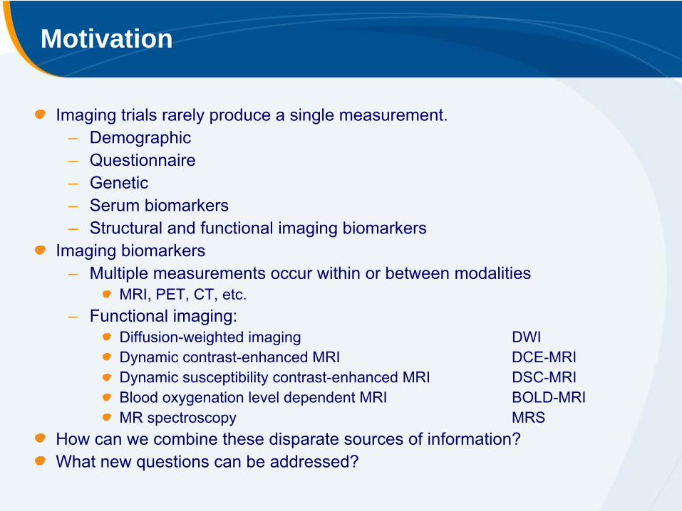
Motivation

Imaging trials rarely produce a single measurement.–

Demographic

–

Questionnaire–

Genetic

–

Serum biomarkers–

Structural and functional imaging biomarkers

Imaging biomarkers–

Multiple measurements occur within or between modalities

MRI, PET, CT, etc.–

Functional imaging:

Diffusion-weighted imaging DWIDynamic contrast-enhanced MRI

DCE-MRIDynamic susceptibility contrast-enhanced MRI

DSC-MRIBlood oxygenation level dependent MRI

BOLD-MRIMR spectroscopy

MRSHow can we combine these disparate sources of information?What new questions can be addressed?

Neuroscience Example

Fig. 1. Voxel-based-morphometry (VBM) analysis showing an additive effect of the APOE ε4 allele (APOE4) on grey matter volume (GMV).

Filippini et al. NeuroImage 2008

Motivation (cont.)

Univariate statistical methods–

One method → one measurement → answer one question

–

One method → multiple measurementsMeasurement #1 → answer question #1Measurement #2 → answer question #1…

Multivariate statistical methods–

Method #1 → one measurement

–

Method #2 → multiple measurements–

Method #3 → multiple measurements

–

…Goal = Prediction (e.g., computer-aided diagnosis)

–

Supervised learning procedures

answer one question

What is Supervised Learning?

Training Data

Supervised Learning Model

Test Data

Results

Step 1

Step 2

T1, T2, DWI, DCE-MRI,

MRS, Genetics

Regression, LDA, SVM,

NN

Benign, malignant

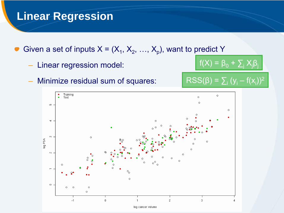
Linear Regression

Given a set of inputs X = (X1

, X2

, …, Xp

), want to predict Y

–

Linear regression model:

–

Minimize residual sum of squares:

f(X) = β0

+ ∑j

Xj

βj

RSS(β) = ∑i

(yi

– f(xi

))2

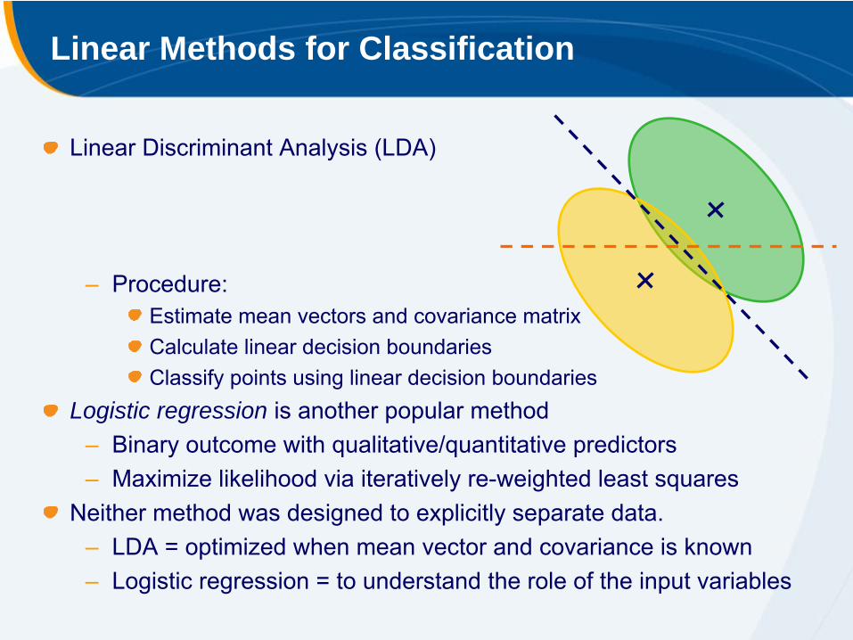
Linear Methods for Classification

Linear Discriminant Analysis (LDA)

–

Procedure:Estimate mean vectors and covariance matrixCalculate linear decision boundariesClassify points using linear decision boundaries

Logistic regression is another popular method–

Binary outcome with qualitative/quantitative predictors

–

Maximize likelihood via iteratively re-weighted least squaresNeither method was designed to explicitly separate data.

–

LDA = optimized when mean vector and covariance is known–

Logistic regression = to understand the role of the input variables

LDA w/ Two Classes: Step-by-Step

Mea

sure

men

t #2

Measurement #1

LDA w/ Three Classes: Step-by-Step

Mea

surin

g #2

Measurement #1

Separating Hyperplanes

Rosenblatt’s Perceptron Learning Algorithm (1958)–

Minimizes the distance of misclassified points to the decision boundary:

–

Converges in a “finite” number of steps.Problems (Ripley, 1996)1.

Separable data implies many solutions (initial conditions).

2.

Slow convergence... smaller the gap = longer the time.3.

Nonseparable data implies the algorithm will not converge!

Optimal separating hyperplanes (Vapnik and Chervonenkis, 1963)–

Forms the foundation for support vector machines.

min D(β,β0

) = –∑iєM yi

(xTβ

+ β0

); yi

= ±1

Separating Hyperplanes: separable case

optimal

Support Vector Machines (Vapnik 1996)

Separates two classes and maximizes the distance to the closest point from either class:

Extends “optimal separating hyperplanes”–

Nonseparable case and nonlinear boundaries

–

Contain a “cost” parameter that may be optimized–

May be used in the regression setting

Basis expansions–

Enlarges the feature space

–

Allowed to get very large or infinite–

Examples include

Gaussian radial basis function (RBF) kernelPolynomial kernelANOVA radial basis kernel

–

Contain a “scaling factor” that may be optimized

max C subject to yi

(xTβ

+ β0

) ≥ C; yi

= ±1

k(x,x′) = exp(-γ║x-x′║2); γ

> 0

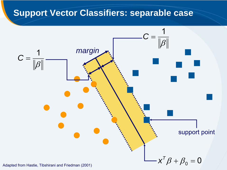
Support Vector Classifiers: separable case

support point

margin

1

C

1

C

Adapted from Hastie, Tibshirani and Friedman (2001)00 Tx

Support Vector Classifiers: nonseparable case

margin

1

C

1

C

Adapted from Hastie, Tibshirani and Friedman (2001)00 Tx

1

2

3

5

4

Support Vector Machine: Spiral Example

Receiver Operating Characteristic (ROC)

Graphical plot of sensitivity vs. (1 –

specificity)–

Binary classifier system as discrimination threshold varies

Sensitivity = True Positive Rate = TP / (TP + FN)Specificity = 1 –

False Positive Rate = 1 –

FP / (FP + TN)

actual value

p n total

prediction outcome

p’True Positive

False Positive P’

n’False Negative

True Negative N’

total P N

2×2 contingency table

Example: Breast Cytology

699 samples–

9 measurements (ordinal)

Clump thicknessCell size uniformityCell shape uniformityMarginal adhesionSingle epithelial cell sizeBare nucleiBland chromatinNormal nucleoliMitoses

–

2 classesBenignMalignant

Classification problem since outcome measure is binary.Train = 550, Test = 133.

Wolberg & Mangasarian (1990)


Diagnostic plot from SVM procedure.


Response surface to SVM parameters.


Logistic RegressionBenign Malignant

Benign 84 5Malignant 4 40

Linear Discriminant AnalysisBenign Malignant


Naïve Support Vector MachineBenign Malignant


Tuned Support Vector MachineBenign Malignant


sensitivity = 98.9%specificity = 85.7%





Receiver operating characteristic (ROC) plot.

Sen

sitiv

ity

1 -

Specificity

Example: Prostate Specific Antigen (PSA)

Stamey et al. (1989); used in Hastie, Tibshirani and Friedman (2001).Correlation between the level of PSA and various clinical measures (N = 97)

–

log cancer volume, –

log prostate weight,

–

log of BPH amount, –

seminal vesicle invasion,

–

log of capsular penetration, –

Gleason score, and

–

percent of Gleason scores 4 or 5.Regression problem since outcome measure is quantitative.Training data = 67, Test data = 30.


Best subset selection for linear regression model.


linear regression model (lcavol, lweight).


Response surface to SVM parameters.


Prediction errors for test data.

Conclusions

Multivariate data are being collected from imaging studies.In order to utilize this information:

–

Use the “right” statistical method–

Collaborate with quantitative scientists

–

Paradigm shift in the analysis of imaging studiesEmbrace the richness of multi-functional imaging data

–

Quantitative–

Raw (avoid summaries)

Design of imaging studies requires–

A priori knowledge

–

Few and focused scientific questions–

Well-defined methodology

Acknowledgments

Anwar PadhaniRoberto AlonziClaire AllenMark EmbertonHenkjan HuismanGiulio Gambarota

Bibliography

Filippini N, Rao, A, et al. Anatomically-distinct genetic associations of APOE ε4 allele load with regional cortical atrophy in Alzheimer's disease. NeuroImage 2009, 44:724-

728.Freer TW, Ulissey, MJ. Screening Mammography with Computer-aided Detection: Prospective Study of 12,860 Patients in a Community Breast Center. Radiology 2001, 220:781-786.Hastie T, Tibshirani, R, Freidman, J. The Elements of Statistical Learning, Springer, 2001.McDonough KL. Breast Cancer Stage Cost Analysis in a Manage Care

Population. American Journal of Managed Care 1999, 5(6):S377-S382.R Development Team. R: A Language and Environment for Statistical Computing. R Foundation for Statistical Computing, Vienna, Austria.

–

www.R-project.org–

R package e1071–

R package mlbenchRipley, BD. Pattern Recognition and Neural Networks, Cambridge University Press, 1996.Vos PC, Hambrock, T, et al. Computerized analysis of prostate lesions in the peripheral zone using dynamic contrast enhanced MRI. Medical Physics 2008, 35(3):888-899.Wolberg WH, Mangasarian, OL. Multisurface method of pattern separation for medical diagnosis applied to breast cytology. PNAS 1990, 87(23):9193-9196.

http://www.r-project.org/

Whitcher Ismrm 2009

Documents

Transcript of Whitcher Ismrm 2009