WhereAreWeNow? Real-Time Estimates of the Macroeconomy

Where Are We Now?

Real-Time Estimates

of the Macroeconomy∗

Martin D.D. EvansGeorgetown University

and the National Bureau of Economic Research

This paper describes a method for calculating daily real-time estimates of the current state of the U.S. economy. Theestimates are computed from data on scheduled U.S. macro-economic announcements using an econometric model that al-lows for variable reporting lags, temporal aggregation, andother complications in the data. The model can be appliedto find real-time estimates of GDP, inflation, unemployment,or any other macroeconomic variable of interest. In this paper,I focus on the problem of estimating the current level of andgrowth rate in GDP. I construct daily real-time estimates ofGDP that incorporate public information known on the dayin question. The real-time estimates produced by the modelare uniquely suited to studying how perceived developmentsin the macroeconomy are linked to asset prices over a widerange of frequencies. The estimates also provide, for the firsttime, daily time series that can be used in practical policydecisions.

JEL Codes: E37, C32.

Information about the current state of real economic activity iswidely dispersed across consumers, firms, and policymakers. Whileindividual consumers and firms know the recent history of their owndecisions, they are unaware of the contemporaneous consumption,

∗I thank an anonymous referee, Jean Imbs, Richard Lyons, Helene Rey, MarkWatson, and the seminar participants at the Federal Reserve Board for valuablecomments. Research on this paper was started while I was a Visiting Fellow at theInternational Economics Section in the Department of Economics at PrincetonUniversity. I thank both the International Economics Section and the NationalScience Foundation for financial support.

127

128 International Journal of Central Banking September 2005

saving, investment, and employment decisions made by other pri-vate sector agents. Similarly, policymakers do not have access toaccurate contemporaneous information concerning private sector ac-tivity. Although information on real economic activity is collected bya number of government agencies, the collection, aggregation, anddissemination process takes time. Thus, while U.S. macroeconomicdata are released on an almost daily basis, the data represent officialaggregations of past rather than current economic activity.

The lack of timely information concerning the current state of theeconomy is well recognized among policymakers. This is especiallytrue in the case of GDP, the broadest measure of real activity. TheFederal Reserve’s ability to make timely changes in monetary pol-icy is made much more complicated by the lack of contemporaneousand accurate information on GDP. The lack of timely informationconcerning macroeconomic aggregates is also important for under-standing private sector behavior and, in particular, the behavior ofasset prices. When agents make trading decisions based on their ownestimate of current macroeconomic conditions, they transmit infor-mation to their trading partners. This trading activity leads to theaggregation of dispersed information and, in the process, affects thebehavior of asset prices. Evans and Lyons (2004a) show that the lackof timely information concerning the state of the macroeconomy cansignificantly alter the dynamics of exchange and interest rates bychanging the trading-based process of information aggregation.

This paper describes a method for estimating the current state ofthe economy on a continual basis using the flow of information froma wide range of macroeconomic data releases. These real-time esti-mates are computed from an econometric model that allows for vari-able reporting lags, temporal aggregation, and other complicationsthat characterize the daily flow of macroeconomic information. Themodel can be applied to find real-time estimates of GDP, inflation,unemployment, or any other macroeconomic variable of interest. Inthis paper, I focus on the problem of estimating GDP in real time.

The real-time estimates derived here are conceptually distinctfrom the real-time data series studied by Croushore and Stark (1999,2001), Orphanides (2001), and others. A real-time data series com-prises a set of historical values for a variable that are known ona particular date. This date identifies the vintage of the real-timedata. For example, the March 31 vintage of real-time GDP data

Vol. 1 No. 2 Real-Time Estimates of the Macroeconomy 129

would include data releases on GDP growth up to the fourth quarterof the previous year. This vintage incorporates current revisions toearlier GDP releases but does not include a contemporaneous esti-mate of GDP growth in the first quarter. As such, it represents asubset of public information available on March 31. By contrast, theMarch 31 real-time estimate of GDP growth comprises an estimateof GDP growth in the first quarter based on information availableon March 31. The real-time estimates derived in this paper use aninformation set that spans the history of data releases on GDP andeighteen other macroeconomic variables.

A number of papers have studied the problem of estimating GDPat a monthly frequency. Chow and Lin (1971) first showed how amonthly series could be constructed from regression estimates us-ing monthly data related to GDP and quarterly GDP data. Thistechnique has been subsequently integrated into VAR forecastingprocedures (see, for example, Robertson and Tallman 1999). Morerecently, papers by Liu and Hall (2000) and Mariano and Murasawa(2003) have used state-space models to combine quarterly GDP datawith other monthly series. The task of calculating real-time estimatesof GDP growth has also been addressed by Kitchen and Monaco(2003). They developed a regression-based method that uses a va-riety of monthly indicators to forecast GDP growth in the currentquarter. The real-time estimates are calculated by combining thedifferent forecasts with a weighting scheme based on the relative ex-planatory power of each forecasting equation.

I differ from this literature by modeling the growth in GDPas the quarterly aggregate of an unobserved daily process for realeconomy-wide activity. The model also specifies the relationship be-tween GDP, data releases on GDP growth, and data releases on a setof other macroeconomic variables in a manner that accommodatesthe complex timing of releases. In particular, I incorporate the vari-able reporting lags that exist between the end of each data collectionperiod (i.e., the end of a month or quarter) and the release day foreach variable. This is only possible because the model tracks theevolution of the economy on a daily basis. An alternative approachof assuming that GDP aggregrates an unobserved monthly processfor economy-wide activity would result in a simpler model structure(see Liu and Hall [2000] and Mariano and Murasawa [2003]), but itcould not accommodate the complex timing of data releases. The


structure of the model also enables me to compute real-time esti-mates of GDP as the solution to an inference problem. In practice,I obtain the real-time estimates as a by-product of estimating themodel. First, the model parameters are estimated by (qausi) max-imum likelihood using the Kalman Filter algorithm. The real-timeestimates are then obtained by applying the algorithm to the modelevaluated at the maximum likelihood estimates (MLEs).

My method for computing real-time estimates has several note-worthy features. First, the estimates are derived from a single fullyspecified econometric model. As such, we can judge the reliability ofthe real-time estimates by subjecting the model to a variety of di-agnostic tests. Second, a wide variety of variables can be computedfrom the estimated model. For example, the model can provide real-time forecasts for GDP growth for any future quarter. It can also beused to compute the precision of the real-time estimates as measuredby the relevant conditional variance. Third, the estimated model canbe used to construct high-frequency estimates of real economic ac-tivity. We can construct a daily series of real-time estimates for GDPgrowth in the current quarter, or real-time estimates of GDP pro-duced in the current month, week, or even day. Fourth, the methodcan incorporate information from a wide range of economic indica-tors. In this paper, I use the data releases for GDP and eighteenother macroeconomic variables, but the set of indicators could beeasily expanded to include many other macroeconomic series andfinancial data. Extending the model in this direction may be par-ticularly useful from a forecasting perspective. Stock and Watson(2002) show that harnessing the information in a large number ofindicators can have significant forecasting benefits.

The remainder of the paper is organized as follows. Section 1 de-scribes the inference problem that must be solved in order to com-pute the real-time estimates. Here I detail the complex timing ofdata collection and macroeconomic data releases that needs to beaccounted for in the model. The structure of the econometric modelis presented in section 2. Section 3 covers estimation and the calcu-lation of the real-time estimates. I first show how the model can bewritten in state-space form. Then I describe how the sample likeli-hood is constructed with the use of the Kalman Filter. Finally, I de-scribe how various real-time estimates are calculated from the maxi-mum likelihood estimates of the model. Section 4 presents the modelestimates and specification tests. Here I compare the forecasting


Figure 1. Data Collection Periods and Release Times forQuarterly and Monthly Variables

Note: The reporting lag for “final” GDP growth in quarter τ , yq(τ),is ry(τ)−q(τ). The reporting lag for the monthly series zm(τ,j) isrz(τ , j)−m(τ , j) for j = 1, 2, 3.

performance of the model against a survey of GDP estimates byprofessional money managers. These private estimates appear com-parable to the model-based estimates even though the managers haveaccess to much more information than the model incorporates. Sec-tion 5 examines the model-based real-time estimates. First, I considerthe relation between the real-time estimates and the final GDP re-leases. Next, I compare alternative real-time estimates for the levelof GDP and examine the forecasting power of the model. Finally, Istudy how the data releases on other macrovariables are related tochanges in GDP at a monthly frequency. Section 6 concludes.

1. Real-Time Inference

My aim is to obtain high-frequency real-time estimates on how themacroeconomy is evolving. For this purpose, it is important to distin-guish between the arrival of information and data collection periods.Information about GDP can arrive via data releases on any day t.GDP data is collected on a quarterly basis. I index quarters by τ anddenote the last day of quarter τ by q(τ), with the first, second, andthird months ending on days m(τ , 1), m(τ , 2), and m(τ , 3), respec-tively. I identify the days on which data is released in two ways. Therelease day for variable κ collected over quarter τ is rκ(τ). Thus,κ

r(τ) denotes the value of variable κ, over quarter τ , released on dayrκ(τ). The release day for monthly variables is identified by rκ(τ , i)for i = 1, 2, 3. In this case, κ

r(τ ,i) is the value of κ, for month iin quarter τ , announced on day rκ(τ , i). The relation between datarelease dates and data collection periods is illustrated in figure 1.


The Bureau of Economic Analysis (BEA) at the U.S. CommerceDepartment releases data on GDP growth in quarter τ in a sequenceof three announcements: the “advanced” growth data are releasedduring the first month of quarter τ + 1; the “preliminary” data arereleased in the second month; and the “final” data are released at theend of quarter τ + 1. The “final” data release does not representthe last official word on GDP growth in the quarter. Each summer,the BEA conducts an “annual” or comprehensive revision that gen-erally leads to revisions in the “final” data values released over theprevious three years. These revisions incorporate more complete anddetailed microdata than was available before the “final” data releasedate.1

Let xq(τ) denote the log of real GDP for quarter τ ending on

day q(τ), and yr(τ) be the “final” data released on day ry(τ). The

relation between the “final” data and actual GDP growth is given by

yr(τ) = ∆qx

q(τ) + υr(τ), (1)

where ∆qxq(τ) ≡ x

q(τ) − xq(τ−1) and υ

a(τ) represents the effect ofthe future revisions (i.e., the revisions to GDP growth made afterry(τ)). Notice that equation (1) distinguishes between the end of thereporting period q(τ) and the release date ry(τ). I shall refer to thedifference ry(τ)−q(τ) as the reporting lag for quarterly data. (Fordata series κ collected during month i of quarter τ , the reportinglag is rκ(τ , i)−m(τ , i).) Reporting lags vary from quarter to quarterbecause data is collected on a calendar basis but announcements arenot made on holidays and weekends. For example, “final” GDP datafor the quarter ending in March has been released between June 27and July 3.

Real-time estimates of GDP growth are constructed using theinformation in a specific information set. Let Ωt denote an informa-tion set that only contains data that is publicly known at the endof day t. The real-time estimate of GDP growth in quarter τ is de-fined as E[∆qx

q(τ)|Ωq(τ)], the expectation of ∆qxq(τ) conditional on

public information available at the end of the quarter, Ωq(τ). To see

how this estimate relates to the “final” data release, y, I combine thedefinition with (1) to obtain

1For a complete description of BEA procedures, see Carson (1987) and Seskinand Parker (1998).


yr(τ) = E

[∆qx

q(τ)|Ωq(τ)

]+ E

[υ

r(τ)|Ωq(τ)

]+

(yr(τ) − E

[yr(τ)|Ωq(τ)

]). (2)

The “final” data released on day ry(τ) comprises three components:the real-time GDP growth estimate; an estimate of future data revi-sions, E

[υ

r(τ)|Ωq(τ)

]; and the real-time forecast error for the data

release, yr(τ)−E

[yr(τ)|Ωq(τ)

]. Under the reasonable assumption that

yr(τ) represents the BEA’s unbiased estimate of GDP growth, and

that Ωq(τ) represents a subset of the information available to the

BEA before the release day, E[υ

r(τ)|Ωq(τ)

]should equal zero. In

this case, (2) becomes

yr(τ) = E

[∆qx

q(τ)|Ωq(τ)

]+

(yr(τ) − E

[yr(τ)|Ωq(τ)

]). (3)

Thus, the data release yr(τ) can be viewed as a noisy signal of the

real-time estimate of GDP growth, where the noise arises from theerror in forecasting y

r(τ) over the reporting lag. By construction,the noise term is orthogonal to the real-time estimate because bothterms are defined relative to the same information set, Ω

q(τ). Thenoise term can be further decomposed as

yr(τ) − E

[yr(τ)|Ωq(τ)

]=

(E

[yr(τ)|Ωbea

q(τ)

]− E

[yr(τ)|Ωq(τ)

])

+(yr(τ) − E

[yr(τ)|Ωbea

q(τ)

]), (4)

where Ωbea

t denotes the BEA’s information set. Since the BEA hasaccess to both private and public information sources, the first termon the right identifies the informational advantage conferred on theBEA at the end of the quarter q(τ). The second term identifies theimpact of new information the BEA collects about x

q(τ) during thereporting lag. Since both of these terms could be sizable, there isno a priori reason to believe that real-time forecast error is alwayssmall.

To compute real-time estimates of GDP, we need to characterizethe evolution of Ωt and describe how inferences about ∆qx

q(τ) can becalculated from Ω

q(τ). For this purpose, I incorporate the informationcontained in the “advanced” and “preliminary” GDP data releases.Let y

r(τ) and yr(τ) respectively denote the values for the “advanced”

and “preliminary” data released on days ry(τ) and ry(τ), where


q(τ) < ry(τ) < ry(τ). I assume that yr(τ) and y

r(τ) represent noisysignals of the “final” data, y

r(τ):

yr(τ) = y

r(τ) + er(τ) + e

r(τ), (5)yr(τ) = y

r(τ) + er(τ), (6)

where er(τ) and e

r(τ) are independent mean zero revision shocks.er(τ) represents the revision between days ry(τ) and ry(τ), and e

r(τ)

represents the revision between days ry(τ) and ry(τ). The idea thatthe provisional data releases represent noisy signals of the “final”data is originally due to Mankiw and Shapiro (1986). It implies thatthe revisions e

r(τ) and er(τ) + e

r(τ) are orthogonal to yr(τ). I im-

pose this orthogonality condition when estimating the model. Thespecification of (5) and (6) also implies that the “advanced” and“preliminary” data releases represent unbiased estimates of actualGDP growth. This assumption is consistent with the evidence re-ported in Faust, Rogers, and Wright (2000) for U.S. data releasesbetween 1988 and 1997. (Adding nonzero means for e

r(τ) and er(τ)

is a straightforward extension to accommodate bias that may bepresent in different sample periods.)2

2It is also possible to accommodate Mankiw and Shapiro’s “news” view ofdata revisions within the model. According to this view, provisional data releasesrepresent the BEA’s best estimate of yr(τ ) at the time the provision data isreleased. Hence yr(τ ) = E[yr(τ )|Ωbea

ry (τ )] and yr(τ ) = E[yr(τ )|Ωbea

ry (τ )]. If the BEA’s

forecasts are optimal, we can write yr(τ ) = yr(τ ) + wr(τ ) and yr(τ ) = yr(τ ) +wr(τ ), where wr(τ ) and wr(τ ) are the forecast errors associated with E[yr(τ )|Ωbea

ry (τ )]

and E[yr(τ )|Ωbea

ry (τ )], respectively. We could use these equations to compute the

projections of yr(τ ) and yr(τ ) on yr(τ ) and a constant:

yr(τ ) = β0 + βyr(τ ) + εr(τ ),

yr(τ ) = β0 + βyr(τ ) + εr(τ ).

The projection errors εr(τ ) and εr(τ ) are orthogonal to yr(τ ) by construction, so

these equations could replace (5) and (6). The projection coefficients, β0, β, β0,

and β, would add to the set of model parameters to be estimated. I chose notto follow this alternative formulation because there is evidence that data revi-sions are forecastable with contemporaneous information (Dynan and Elmendorf2001). This finding is inconsistent with the “news” view if the BEA makes ra-tional forecasts. Furthermore, as I discuss below, a specification based on (5)and (6) allows the optimal (model-based) forecasts of “final” GDP to closelyapproximate the provisional data releases. The model estimates will thereforeprovide us with an empirical perspective on the “noise” and “news” characteri-zations of data revisions.


The three GDP releases yr(τ), y

r(τ), yr(τ) represent a sequence

of signals on actual GDP growth that augment the public infor-mation set on days ry(τ), ry(τ), and ry(τ). In principle, we couldconstruct real-time estimates based only on these data releases asE[∆qx

q(τ)|Ωyq(τ)], where Ωy

t is the information set comprising dataon the three GDP series released on or before day t:

Ωyt ≡

yr(τ), yr(τ), yr(τ) : r(τ) < t

.

Notice that these estimates are only based on data releases relatingto GDP growth before the current quarter because the presence of thereporting lags excludes the values of y

r(τ), yr(τ), and y

r(τ) from Ωq(τ).

As such, these candidate real-time estimates exclude information on∆qx

q(τ) that is available at the end of the quarter. Much of thisinformation comes from the data releases on other macroeconomicvariables like employment, retail sales, and industrial production.Data for most of these variables are collected on a monthly basis3

and, as such, can provide timely information on GDP growth. Tosee why this is so, consider the data releases on nonfarm payrollemployment, z. Data on z for the month ending on day mz(τ , j) arereleased on rz(τ , j), a day that falls between the third and the ninthof month j +1 (as illustrated in figure 1). This reporting lag is muchshorter than the lag for GDP releases but it does exclude the useof employment data from the third month in estimating real-timeGDP. However, insofar as employment during the first two monthsis related to GDP growth over the quarter, the values of z

r(τ ,1) andzr(τ ,2) will provide information relevant to estimating GDP growth

at the end of the quarter.The real-time estimates I construct below will be based on data

from the three GDP releases and the monthly releases of othermacroeconomic data. To incorporate the information from theseother variables, I decompose quarterly GDP growth into a sequenceof daily increments:

∆qxq(τ) =

d(τ)∑i=1

∆xq(τ−1)+i, (7)

3Data on initial unemployment claims are collected week by week.


where d(τ) ≡ q(τ)−q(τ − 1) is the duration of quarter τ . The dailyincrement ∆xt represents the contribution on day t to the growthof GDP in quarter τ . If xt were a stock variable, like the log pricelevel on day t, ∆xt would identify the daily growth in the stock (e.g.,the daily rate of inflation). Here x

q(τ) denotes the log of the flow ofoutput over quarter τ , so it is not appropriate to think of ∆xt as thedaily growth in GDP. I will examine the link between ∆xt and dailyGDP in section 3.3 below.

To incorporate the information contained in the ith macrovari-able, zi, I project zi

r(τ ,j) on a portion of GDP growth

zir(τ ,j) = βi∆

mxm(τ ,j) + ui

m(τ ,j), (8)

where ∆mxm(τ ,j) is the contribution to GDP growth in quarter τ

during month j:

∆mxm(τ ,j) ≡

m(τ ,j)∑i=m(τ,j−1)+1

∆xi.

βi is the projection coefficient and uim(τ ,j) is the projection error that

is orthogonal to ∆mxm(τ ,j). Notice that equation (8) incorporates

the reporting lag rz(τ , j)−mz(τ , j) for variable z, which can vary inlength from month to month.

The real-time estimates derived in this paper are based on aninformation set specification that includes the three GDP releasesand eighteen monthly macro series: zi = 1, 2, . . . , 18. Formally, Icompute the end-of-quarter real-time estimates as

E[∆qxq(τ)|Ωq(τ)], (9)

where Ωt = Ωzt ∪Ωy

t , with Ωzt denoting the information set comprising

data on the eighteen monthly macrovariables that has been releasedon or before day t:

Ωzt ≡

⋃18i=1

zir(τ ,j) : r(τ , j) < t for j = 1, 2, 3

.

The model presented below enables us to compute the real-timeestimates in (9) using equations (1), (5), (6), (7), and (8) together


with a time-series process for the daily increments, ∆xt. The modelwill also enable us to compute daily real-time estimates of quarterlyGDP, and GDP growth:

xq(τ)|i ≡ E[x

q(τ)|Ωi] (10)

∆qxq(τ)|i ≡ E[∆qx

q(τ)|Ωi] (11)

for q(τ − 1) < i ≤ q(τ). Equations (10) and (11) respectivelyidentify the real-time estimate of log GDP, and GDP growth inquarter τ , based on information available on day i during thequarter. x

q(τ)|i and ∆qxq(τ)|i incorporate real-time forecasts of the

daily contribution to GDP in quarter τ between day i and q(τ).These high-frequency estimates are particularly useful in studyinghow data releases affect estimates of the current state of the econ-omy, and forecasts of how it will evolve in the future. As such, theyare uniquely suited to examining how data releases affect a wholearray of asset prices.

2. The Model

The dynamics of the model center on the behavior of two partialsums:

sq

t ≡minq(τ),t∑i=q(τ)+1

∆xi, (12)

sm

t ≡minm(τ,j),t∑i=m(τ,j−1)+1

∆xi. (13)

Equation (12) defines the cumulative daily contribution to GDPgrowth in quarter τ , ending on day t ≤ q(τ). The cumulativedaily contribution between the start of month j in quarter τ andday t is defined by sm

t . Notice that when t is the last day of thequarter, ∆qx

q(τ) = sq

q(τ), and when t is the last day of month j,∆mx

m(τ,j) = sm

m(τ ,j). To describe the daily dynamics of sq

t and sm

t , Iintroduce the following dummy variables:


λm

t =

1 if t = m(τ , j) + 1, for j = 1, 2, 3,

0 otherwise,

λq

t =

1 if t = q(τ) + 1,

0 otherwise.

Thus, λm

t and λq

t take the value of one if day t is the first day ofthe month or quarter, respectively. We may now describe the dailydynamics of sq

t and sm

t with the following equations:

sq

t =(1 − λq

t

)sq

t−1 + ∆xt, (14)

sm

t = (1 − λm

t ) sm

t−1 + ∆xt. (15)

The next portion of the model accommodates the reporting lags.Let ∆q(j)xt denote the quarterly growth in GDP ending on day q(τ−j), where q(τ) denotes the last day of the most recently completedquarter and t ≥ q(τ). Quarterly GDP growth in the last (completed)quarter is given by

∆q(1)xt =(1 − λq

t

)∆q(1)xt−1 + λq

t sq

t−1. (16)

When t is the first day of a new quarter, λq

t = 1, so ∆q(1)xq(τ)+1 =

sq

q(t) = ∆qxq(τ). On all other days, ∆q(1)xt = ∆q(1)xt−1. On some

dates, the reporting lag associated with a “final” GDP data release ismore than one quarter, so we will need to identify GDP growth fromtwo quarters back, ∆q(2)xt. This is achieved with a similar recursion:

∆q(2)xt =(1 − λq

t

)∆q(2)xt + λq

t ∆q(1)xt−1. (17)

Equations (14), (16), and (17) enable us to define the link be-tween the daily contributions to GDP growth ∆xt and the threeGDP data releases yt, yt, yt . Let us start with the “advanced”GDP data releases. The reporting lag associated with these datais always less than one quarter, so we can combine (1) and (5) withthe definition of ∆q(1)xt to write

yt = ∆q(1)xt + υr(τ) + e

r(τ) + er(τ). (18)


It is important to recognize that (18) builds in the variable reportinglag between the release day, ry(τ), and the end of the last quarterq(τ). The value of ∆q(1)xt does not change from day to day afterthe quarter ends, so the relation between the data release and actualGDP growth is unaffected by within-quarter variations in the report-ing lag. The reporting lag for the “preliminary” data is also alwaysless than one quarter. Combining (1) and (6) with the definition of∆q(1)xt, we obtain

yt = ∆q(1)xt + υr(τ) + e

r(τ). (19)

Data on “final” GDP growth is released around the end of the fol-lowing quarter, so the reporting lag can vary between one and twoquarters. In cases where the reporting lag is one quarter,

yt = ∆q(1)xt + υr(τ), (20)

and when the lag is two quarters,

yt = ∆q(2)xt + υr(τ). (21)

I model the links between the daily contributions to GDP growthand the monthly macrovariables in a similar manner. Let ∆m(i)xt

denote the monthly contribution to quarterly GDP growth endingon day m(τ , j − i), where m(τ , j) denotes the last day of the mostrecently completed month and t ≥ m(τ , j). The contribution to GDPgrowth in the last (completed) month is given by

∆m(1)xt = (1 − λm

t ) ∆m(1)xt−1 + λm

t sm

t−1, (22)

and the contribution from i (> 1) months back is

∆m(i)xt = (1 − λm

t ) ∆m(i)xt + λm

t ∆m(i−1)xt−1. (23)

These equations are analogous to (16) and (17). If t is the first dayof a new month, λm

t = 1, so ∆m(1)xm(τ ,j)+1 = sq

m(τ,j) = ∆mxm(τ ,j)

and ∆m(i)xm(τ ,j)+1 = ∆m(i−1)x

m(τ ,j) for j = 1, 2, 3. On all other days,∆m(i)xt = ∆m(i)xt−1. The ∆m(i)xt variables link the monthly datareleases, zi

t, to quarterly GDP growth. If the reporting lag for macro


series i is less than one month, the value released on day t can bewritten as

zit = βi∆

m(1)xt + uit. (24)

In cases where the reporting lag is two months,

zit = βi∆

m(2)xt + uit. (25)

As above, both equations allow for a variable within-month reportinglag, rzi(τ , j)−mzi(τ , j).

Equations (24) and (25) accommodate all the monthly data re-leases I use except for the index of consumer confidence, i = 18. Thisseries is released before the end of the month in which the surveydata are collected. These data are potentially valuable for drawingreal-time inferences because they represent the only monthly releasebefore q(τ) that relates to activity during the last month of the quar-ter. I incorporate the information in the consumer confidence index(i = 18) by projecting z18

t on the partial sum sm

t :

z18t = β18s

m

t + u18t . (26)

To complete the model, we need to specify the dynamics for thedaily contributions, ∆xt. I assume that

∆xt =k∑

i=1

φi∆m(i)xt + et, (27)

where et is an i.i.d.N(0, σ2e) shock. Equation (27) expresses the

growth contribution on day t as a weighted average of the monthlycontributions over the last k (completed) months, plus an error term.This specification has two noteworthy features. First, the daily con-tribution on day t only depends on the history of ∆xt insofar asit is summarized by the monthly contributions, ∆m(i)xt. Thus, fore-casts for ∆xt+h conditional

∆m(i)xt

k

i=1are the same for horizons h

within the current month. The second feature of (27) is that the proc-ess aggregates up to an AR(k) process for ∆mx

m(τ ,j) at the monthlyfrequency. As I shall demonstrate, this feature enables us to computereal-time forecasts of future GDP growth over monthly horizons withcomparative ease.


3. Estimation

Finding the real-time estimates of GDP and GDP growth requiresa solution to two related problems. First, there is a pure inferenceproblem of how to compute E[x

q(τ)|Ωi] and E[∆qxq(τ)|Ωi] using the

quarterly signaling equations (18)–(21), the monthly signaling equa-tions (24)–(26), and the ∆xt process in (27), given values for all theparameters in these equations. Second, we need to estimate theseparameters from the three data releases on GDP and the eighteenother macro series. This problem is complicated by the fact thatindividual data releases are irregularly spaced and arrive in a non-synchronized manner: on some days there is one release, on othersthere are several, and on some there are none at all. In short, thetemporal pattern of data releases is quite unlike that found in stan-dard time-series applications.

The Kalman Filtering algorithm provides a solution to both prob-lems. In particular, given a set of parameter values, the algorithmprovides the means to compute the real-time estimates E[x

q(τ)|Ωi]and E[∆qx

q(τ)|Ωi]. The algorithm also allows us to construct a sam-ple likelihood function from the data series, so that the model’s pa-rameters can be computed by maximum likelihood. Although theKalman Filtering algorithm has been used extensively in the ap-plied time-series literature, its application in the current context hasseveral novel aspects. For this reason, the presentation below con-centrates on these features.4

3.1 The State-Space Form

To use the algorithm, we must first write the model in state-spaceform comprising a state and observation equation. For the sake ofclarity, I shall present the state-space form for the model where ∆xt

depends only on last month’s contribution (i.e., k = 1 in equation[27]). Modifying the state-space form for the case where k > 1 isstraightforward.

4For a textbook introduction to the Kalman Filter and its uses in standardtime-series applications, see Harvey (1989) or Hamilton (1994).


The dynamics described by equations (14)–(17), (22), (23), and(27) with k = 1 can be represented by the matrix equation:

sq

t

∆q(1)xt

∆q(2)xt

sm

t

∆m(1)xt

∆m(2)xt

∆xt

=

1 − λq

t 0 0 0 0 0 1

λq

t 1 − λq

t 0 0 0 0 0

0 λq

t 1 − λq

t 0 0 0 0

0 0 0 1 − λm

t 0 0 1

0 0 0 λm

t 1 − λm

t 0 0

0 0 0 0 λm

t 1 − λm

t 0

0 0 0 0 φ1 0 0

×

sq

t−1

∆q(1)xt−1

∆q(2)xt−1

sm

t−1

∆m(1)xt−1

∆m(2)xt−1

∆xt−1

+

0

0

0

0

0

0

et

,

or, more compactly,

Zt = AtZt−1 + Vt. (28)

Equation (28) is known as the state equation. In traditional time-series applications, the state transition matrix A is constant. Hereelements of At depend on the quarterly and monthly dummies, λq

t

and λm

t , and so At is time varying.Next, we turn to the observation equation. The link between the

data releases on GDP and elements of the state vector are describedby (18), (19), (20), and (21). These equations can be rewritten as


yt

yt

yt

=

0 ql1t (y) ql

2t (y) 0 0 0 0

0 ql1t (y) ql

2t (y) 0 0 0 0

0 ql1t (y) ql

2t (y) 0 0 0 0

Zt

+

1 1 1

0 1 1

0 0 1

et

et

υt

, (29)

where qlit(κ) denotes a dummy variable that takes the value of one

when the reporting lag for series κ lies between i − 1 and i quar-ters, and zero otherwise. Thus, ql

1t (y) = 1 and ql

2t (y) = 0 when

“final” GDP data for the first quarter are released before the startof the third quarter, while ql

1t (y) = 0 and ql

2t (y) = 1 in cases where

the release is delayed until the third quarter. Under normal circum-stances, the “advanced” and “preliminary” GDP data releases havereporting lags that are less than a month. However, there was oneoccasion in the sample period where all the GDP releases were de-layed, so that the ql

it(κ) dummies are also needed for the yt and yt

equations.The link between the data releases on the monthly series and ele-

ments of the state vector is described by (24)–(26). These equationscan be written as

zit =

[0 0 0 βiml

0t (z

i) βiml1t (z

i) βiml2t (z

i) 0]

Zt + uit,

(30)

for i = 1, 2, . . . , 18. mlit(κ) is the monthly version of ql

it(κ). ml

it(κ)

is equal to one if the reporting lag for series κ lies between i− 1 andi months (i = 1, 2), and zero otherwise. ml

0t (κ) equals one when the

release day is before the end of the collection month (as is the casewith the index of consumer confidence). Stacking (29) and (30) gives


yt

yt

yt

z1t

...

z18t

=

0 ql1t (y) ql

2t (y) 0 0 0 0

0 ql1t (y) ql

2t (y) 0 0 0 0

0 ql1t (y) ql

2t (y) 0 0 0 0

0 0 0 β1ml0t (z

1) βiml1t (z

1) β1ml2t (z

1) 0...

......

......

......

0 0 0 β18ml0t (z

18) β18ml1t (z

18) β18ml2t (z

18) 0

Zt

+

et + et + υt

et + υt

υt

u1t

...

u18t

,

or

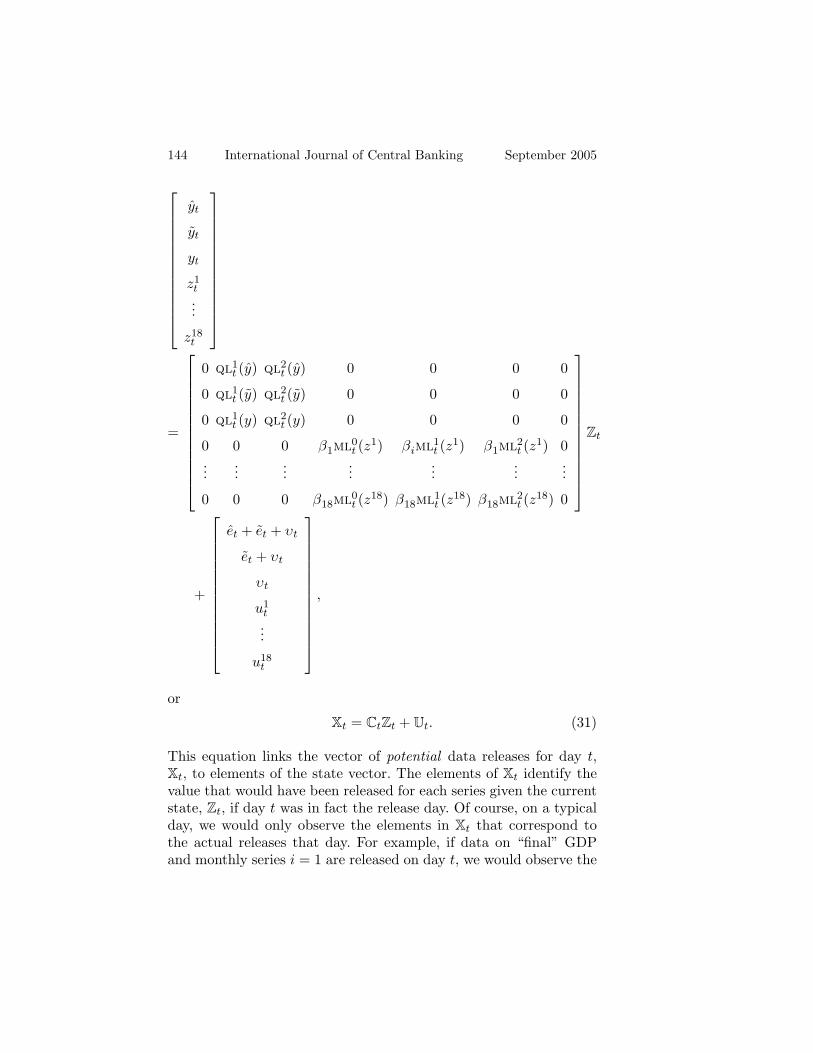
Xt = CtZt + Ut. (31)

This equation links the vector of potential data releases for day t,Xt, to elements of the state vector. The elements of Xt identify thevalue that would have been released for each series given the currentstate, Zt, if day t was in fact the release day. Of course, on a typicalday, we would only observe the elements in Xt that correspond tothe actual releases that day. For example, if data on “final” GDPand monthly series i = 1 are released on day t, we would observe the


values in the third and fourth rows of Xt. On days when there areno releases, none of the elements of Xt are observed.

The observation equation links the data releases for day t to thestate vector. The vector of actual data releases for day t, Yt, is relatedto the vector of potential releases by

Yt = BtXt,

where Bt is an n × 21 selection matrix that “picks out” the n ≥ 1data releases for day t. For example, if data on monthly series i = 1are released on day t, Bt = [ 0 0 0 1 0, . . . . . , 0 ]. Combiningthis expression with (31) gives the observation equation:

Yt = BtCtZt + BtUt. (32)

Equation (32) differs in several respects from the observationequation specification found in standard time-series applications.First, the equation only applies on days for which at least one datarelease takes place. Second, the link between the observed data re-leases and the state vector varies through time via Ct as ql

it(κ)

and mlit(κ) change. These variations arise because the reporting lag

associated with a given data series change from release to release.Third, the number and nature of the data releases vary from dayto day (i.e., the dimension of Yt can vary across consecutive data-release days) via the Bt matrix. These changes may be a source ofheteroskedasticity. If the Ut vector has a constant covariance matrixΩu, the vector of noise terms entering the observation equation willbe heteroskedastic with covariance BtΩuB

′t.

3.2 The Kalman Filter and Sample LikelihoodFunction

Equations (28) and (32) describe a state-space form that can beused to find real-time estimates of GDP in two steps. In the first, Iobtain the maximum likelihood estimates of the model’s parameters.The second step calculates the real-time estimates of GDP using themaximum likelihood parameter estimates. Below, I briefly describethese steps, noting where the model gives rise to features that arenot seen in standard time-series applications.

The parameters of the model to be estimated are θ =β1, . . . , β21, φ1, . . . , φk, σ2

e, σ2e, σ

2e, σ2

v, σ21, . . . , σ

218, where σ2

e, σ2e, σ2

e,


and σ2v denote the variances of et, et, et, and υt, respectively. The

variance of uit is σ2

i for i = 1, . . . , 18. For the purpose of estimation,I assume that all variances are constant, so the covariance matricesfor Vt and Ut can be written as Σv and Σu, respectively. The samplelikelihood function is built up recursively by applying the KalmanFilter to (28) and (32). Let nt denote the number of data releaseson day t. The sample log likelihood function for a sample spanningt = 1, . . . , T is

L(θ) =T∑

t=1,nt>0

−nt

2ln (2π) − 1

2ln |ωt| − 1

2η′tω

−1t ηt

, (33)

where ηt denotes the vector of innovations on day t with nt > 0, andωt is the associated conditional covariance matrix. The ηt and ωt

sequences are calculated as functions of θ from the filtering equations:

Zt|t = AtZt−1|t−1 + Ktηt, (34a)

St+1|t = At (I − KtBtCt) St|t−1A′t + Σv, (34b)

where

ηt = Yt − BtCtAtZt−1|t−1, (35a)

Kt = St|t−1C′tB

′tω

−1t , (35b)

ωt = BtCtSt|t−1C′tB

′t + BtΣuB

′t, (35c)

if nt > 0, and

Zt|t = AtZt−1|t−1, (36a)

St+1|t = AtSt|t−1A′t + Σv, (36b)

when nt = 0. The recursions are initialized with S1|0 = Σv andZ0|0 equal to a vector of zeros. Notice that (34)–(36) differ from thestandard filtering equations because the structure of the state-spaceform in (28) and (32) changes via the At, Ct, and Bt matrices. Thefiltering equations also need to account for the days on which nodata is released.

As in standard applications of the Kalman Filter, we need toensure that all the elements of θ are identified. Recall that equation


(1) includes an error term υt to allow for annual revisions to the“final” GDP data that take place after the release day ry(τ). Thevariance of υt, σ2

v, is not identified because the state-space formexcludes data on the annual revisions. Rather than amend the modelto include these data, I impose the identifying restriction: σ2

v = 0.5

This restriction limits the duration of uncertainty concerning GDPgrowth to the reporting lag for the “final” GDP release. In section5, I show that most of the uncertainty concerning GDP growth inquarter τ is resolved by the end of the first month in quarter τ + 1,well before the end of the reporting lag. Limiting the duration ofuncertainty does not appear unduly restrictive.

3.3 Calculating the Real-Time Estimates of GDP

Once the maximum likelihood estimates of θ have been found, theKalman Filtering equations can be readily used to calculate real-time estimates of GDP. Consider, first, the real-time estimates atthe end of each quarter ∆qx

q(τ)|q(τ). By definition, Zt|j denotes theexpectation of Zt conditioned on data released by the end of day j,E[Zt|Ωj ]. Hence, the real-time estimates of quarterly GDP growthare given by

∆qxq(τ)|q(τ) = E[sq

q(τ)|Ωq(τ)] = h1Zq(τ)|q(τ), (37)

for τ = 1, 2, . . . , where hi is a vector that selects the ith element of Zt.Zt|t denotes the value of Zt|t based on the MLE of θ computed from(34)–(36). The Kalman Filter allows us to study how the estimatesof ∆qx

q(τ) change in the light of data releases after the quarter hasended. For example, the sequence ∆qx

q(τ)|t = h2Zt|t, for q(τ) <t ≤q(τ + 1), shows how data releases between the end of quarters τand τ + 1 change the real-time estimates of ∆qx

q(τ).

5In principle, the state-space form could be augmented to accommodate therevision data, but the resulting state vector would have forty-odd elements be-cause revisions can take place up to three years after the “final” GDP data isreleased. Estimating such a large state-space system would be quite challenging.Alternatively, one could estimate σ2

v directly from the various vintages of “fi-nal” growth rates for each quarter, and then compute the maximum likelihoodestimates of the other parameters conditioned on this value.


We can also use the model to find real-time estimates of GDPgrowth before the end of the quarter. Recall that quarterly GDPgrowth can be represented as the sum of daily increments:

∆qxq(τ) =

d(τ)∑i=1

∆xq(τ−1)+i. (7)

Real-time estimates of ∆qxq(τ) based on information Ωt, where q(τ−

1) < t ≤ q(τ), can be found by taking conditional expectations onboth sides of this equation:

∆qxq(τ)|t = E[sq

t |Ωt] +q(τ)∑h=1

E[∆xt+h|Ωt]. (38)

The first term on the right-hand side is the real-time estimate ofthe partial sum sq

t defined in (12). Since sq

t is the first elementin the state vector Zt, a real-time estimate of sq

t can be found asE[sq

t |Ωt] = h1Zt|t. The second term in (38) contains real-time fore-casts for the daily increments over the remaining days in the month.These forecasts can be easily computed from the process for the in-crements in (27):

E[∆xt+h|Ωt] =k∑

i=1

φiE[∆m(i)xt|Ωt]. (39)

Notice that the real-time estimates of ∆m(i)xt on the right-hand sideare also elements of the state vector Zt, so the real-time forecasts canbe easily found from Zt|t. For example, for the state-space form withk = 1 described above, the real-time estimates can be computed as∆qx

q(τ)|t =[h1 + h5φ1(q(τ) − t)

]Zt|t, where φ1 is the MLE of φ1.

The model can also be used to calculate real-time estimates oflog GDP, x

q(τ)|i. Once again, it is easiest to start with the end-of-quarter real-time estimates, x

q(τ)|q(τ). Iterating on the identity∆qx

q(τ) ≡ xq(τ) − x

q(τ−1), we can write

xq(τ) =

τ∑i=1

∆qxq(i) + x

q(0). (40)


Thus, log GDP for quarter τ can be written as the sum of quarterlyGDP growth from quarters 1 to τ , plus the initial log level of GDPfor quarter 0. Taking conditional expectations on both sides of thisexpression gives

xq(τ)|q(τ) =

τ∑i=1

E[∆qxq(i)|Ωq(τ)] + E[x

q(0)|Ωq(τ)]. (41)

Notice that the terms in the sum on the right-hand side are not thereal-time estimates of GDP growth. Rather, they are current esti-mates (i.e., based on Ω

q(τ)) of past GDP growth. Thus, we cannotconstruct real-time estimates of log GDP by simply aggregating thereal-time estimate of GDP growth from the current and past quar-ters.

In principle, xq(τ)|q(τ) could be found using estimates of

E[∆qxq(i)|Ωq(τ)] computed from the state-space form with the aid of

the Kalman Smoother algorithm (see, for example, Hamilton 1994).An alternative approach is to apply the Kalman Filter to a modifiedversion of the state-space form:

Zat = A

at Z

at + V

at , (42a)

Yt = BtCat Z

at + BtUt, (42b)

where

Zat ≡

Zt

xt

, A

at ≡

At 0

h7 1

, V

at =

I7

h7

Vt, and

Cat ≡

[Ct 0

].

This modified state-space form adds the cumulant of the daily in-crements, xt ≡

∑ti=1 ∆xi + x

q(0), as the eighth element in the aug-mented state vector Z

at . At the end of the quarter when t =q(τ), the

cumulant is equal to xq(τ). So a real-time end-of-quarter estimate of

log GDP can be computed as xq(τ)|q(τ) = ha

8Zaq(τ)|q(τ), where Z

at|t is

the estimate of Zat derived by applying that Kalman Filter to (42),

and hai is a vector that picks out the ith element of Z

at .

Real-time estimates of log GDP in quarter τ based on informationavailable on day t < q(τ) can be calculated in a similar fashion. First,we use (7) and the definition of xt to rewrite (40) as


xq(τ) = xt +

q(τ)∑h=t+1

∆xh.

As above, the real-time estimate is found by taking conditional ex-pectations:

xq(τ)|t = E[xt|Ωt] +

q(τ)∑h=t+1

E[∆xh|Ωt]. (43)

The real-time estimate of log GDP for quarter τ , based on informa-tion available on day t ≤Q(τ), comprises the real-time estimate ofxt and the sum of the real-time forecasts for ∆xt+h over the remain-der of the quarter. Notice that each component on the right-handside was present in the real-time estimates discussed above, so find-ing x

q(τ)|t involves nothing new. For example, in the k = 1 case,x

q(τ)|t = [ha8 + ha

5φ1 (q(τ) − t)]Zat|t.

To this point, I have concentrated on the problem of calculatingreal-time estimates for GDP and GDP growth measured on a quar-terly basis. We can also use the model to calculate real-time estimatesof output flows over shorter horizons, such as a month or week. Forthis purpose, I first decompose quarterly GDP into its daily compo-nents. These components are then aggregated to construct estimatesof output measured over any horizon.

Let dt denote the log of output on day t. Since GDP for quarterτ is simply the aggregate of daily output over the quarter,

xq(τ) ≡ ln

(∑d(τ)

i=1exp

(dq(τ−1)+i

)), (44)

where d(τ) ≡ q(τ)−q(τ − 1) is the duration of quarter τ . Equa-tion (44) describes the exact nonlinear relation between log GDP forquarter τ and the log of daily output. In principle, we would like touse this equation and the real-time estimates of x

q(τ) to identify thesequence for dt over each quarter. Unfortunately, this is a form ofnonlinear filtering problem that has no exact solution. Consequently,to make any progress, we must work with either an approximate so-lution to the filtering problem or a linear approximation of (44).


I follow the second approach by working with a first-order Taylorapproximation to (44) around the point where dt = x(τ) − lnd(τ):

xq(τ)

∼= 1d(τ)

d(τ)∑i=1

dq(τ−1)+i + lnd(τ)

. (45)

Combining (45) with the identity ∆qxq(τ) ≡ x

q(τ) − xq(τ−1) gives

∆qxq(τ)

∼= 1d(τ)

d(τ)∑i=1

dq(τ−1)+i −

(x

q(τ−1) − lnd(τ))

. (46)

This expression takes the same form as the decomposition of quar-terly GDP growth in (7) with ∆xt

∼=dt − x

q(τ−1) + lnd(τ)

/d(τ).Rearranging this expression gives us the following approximation forlog daily output:

dt∼= x

q(τ−1) + d(τ)∆xt − lnd(τ). (47)

According to this approximation, all the within-quarter variationin the log of daily output is attributable to daily changes in theincrements ∆xt. Thus, changes in xt within each quarter provide anapproximate (scaled) estimate of the volatility in daily output.

The last step is to construct the new output measure based on(47). Let xh

t denote the log flow of output over h days ending onday t: xh

t ≡ ln(∑h−1

i=0 exp (dt−i)). As before, I avoid the problems

caused by the nonlinearity in this definition by working with a first-order Taylor approximation to xh

t around the point where dt = xht −

lnh. Combining this approximation with (47) and taking conditionalexpectations gives

xht|t

∼= 1h

h−1∑i=1

E[x

q(τ t−i−1)|Ωt] + d(τ t−i)E[∆xt−i|Ωt]

− lnd(τ t−i) + lnh , (48)

where τ t denotes the quarter in which day t falls. Equation (48)provides us with an approximation for the real-time estimates ofxh

t in terms that can be computed from the model. In particular,if we augment the state vector to include x

q(τ t−i−1) and ∆xt−i for


i = 1, . . . , h − 1, and apply the Kalman Filter to the resulting mod-ified state space, the estimates of E[x

q(τ t−i−1)|Ωt] and E[∆xt−i|Ωt]can be constructed from Z

at|t.

4. Empirical Results

4.1 Data

The macroeconomic data releases used in estimation are from In-ternational Money Market Services (MMS). These include real-timedata on both expected and announced macrovariables. I estimate themodel using the three quarterly GDP releases and the monthly re-leases on eighteen other variables from April 11, 1993, through June30, 1999. In specification tests described below, I also use marketexpectations of GDP growth based on surveys conducted by MMSof approximately forty money managers on the Friday of the weekbefore the release day. Many earlier studies have used MMS data toconstruct proxies for the news contained in data releases (see, forexample, Urich and Watchel 1984; Balduzzi, Elton, and Green 2001;and Andersen et al. 2003). This is the first paper to use MMS datain estimating real-time estimates of macroeconomic variables.

The upper panel of table 1 lists the data series used in estima-tion. The right-hand columns report the number of releases and therange of the reporting lag for each series during the sample period.The lower panel shows the distribution of data releases. The sam-ple period covers 1,682 workdays (i.e., all days excluding weekendsand national holidays).6 On approximately 55 percent of these days,there was at least one data release. Multiple data releases occurredmuch less frequently, on approximately 16 percent of the workdaysin the sample. There were no occasions when more than four datareleases took place.

The release data were transformed in two ways before being in-corporated in the model. First, I subtracted the sample mean from

6Although economic activity obviously takes place on weekends and holidays,I exclude these days from the sample for two reasons. First, they contain no datareleases. This means that the contribution to GDP on weekends and holidaysmust be exclusively derived from the dynamics of (27). Second, by including onlyworkdays, we can exactly align the real-time estimates with days on which U.S.financial markets were open. This feature will be very helpful in studying therelation between the real-time estimates and asset prices.


Table 1. Data Series (April 11, 1993–June 30, 1999)

Release Obs. Reporting Lag

Quarterly Advanced GDP 26 1–2 Months

Preliminary GDP 25 2–3 Months

Final GDP 26 3–4 Months

Monthly

Real Activity Nonfarm Payroll Employment 78 3–9 Days

Retail Sales 78 12–15 Days

Industrial Production 78 15–18 Days

Capacity Utilization 78 15–18 Days

Personal Income 76 30–33 Days

Consumer Credit 78 33–40 Days

Consumption Personal Consumption 76 30–33 Days

Expenditures

New Home Sales 77 27–33 DaysInvestment Durable Goods Orders 77 24–29 Days

Construction Spending 77 31–34 Days

Factory Orders 76 29–35 Days

Business Inventories 78 38–44 Days

Government Government Budget Deficit 78 15–21 Days

Net Exports Trade Balance 78 44–53 Days

Forward Looking Consumer Confidence Index 78 –8–0 Days

NAPM Index 78 0–6 Days

Housing Starts 77 14–20 Days

Index of Leading Indicators 78 27–45 Days

Distribution of Data Releases

Releases per Day Fraction of Sample Observations

0 45.48% 765

1 38.76% 652

2 10.46% 176

3 4.34% 73

4 0.95% 16

> 0 54.52% 917

each of the GDP releases. This transformation implies that the real-time estimates presented below are based on the assumption thatlong-run GDP growth remained constant over the sample period. Ifthe span of my data were considerably longer, I could identify howthe long-run rate of GDP growth has varied by estimating a modifiedform of the model that replaced (27) with a process that decomposed∆xt into short- and long-run components. I leave this extension ofthe model for future work.


The second transformation concerns the monthly data. Let zir(τ ,j)

denote the raw value for series i released on day t =r(τ , j). Themodel incorporates transformed series zi

r(τ ,j) = (zir(τ ,j) − zi) −

αi(zir(τ ,j−1) − zi), where zi is the sample mean of zi. Recall that

in the model, the monthly series provide noisy signals on themonthly contribution to GDP growth (see equations [24]–[26]).Quasi-differencing in this manner allows each of the raw data se-ries to have a differing degree of persistence than the monthly con-tribution to GDP growth without inducing serial correlation in theprojection errors shown in (24)–(26). The degree of quasi-differencingdepends on the αi parameters which are jointly estimated with theother model parameters.

4.2 Estimates and Diagnostics

The maximum likelihood estimates of the model are reported intable 2. There are sixty-three parameters in the model, and all areestimated with a great deal of precision. T-tests based on the asymp-totic standard errors (reported in parentheses) show that all thecoefficients are significant at the 1 percent level. Panel A of the ta-ble shows the estimated parameters of the daily contribution proc-ess in (27). Notice that the reported estimates and standard er-rors are multiplied by twenty-five. With this scaling, the reportedvalues for the φi parameters represent the coefficients in the time-aggregated AR(6) process for ∆Mx

M(τ ,j) in a typical month (i.e., onewith twenty-five workdays). I shall examine the implications of theseestimates for forecasting GDP below.

Panel B reports the estimated standard deviations of the differ-ence between the “advanced” and “final” GDP releases, ωa ≡ yt−yt,and the difference between the “preliminary” and “final” releases,ωp ≡ yt − yt. According to equations (5) and (6) of the model,V(ωa) = V(ωp)+V(e

r(τ)), so the standard deviation of ωa should beat least as great as that of ωp. By contrast, the estimates in panelB imply that V(ωa) < V(ωp).

7 This suggests that revisions the BEAmade between releasing the “preliminary” and “final” GDP datawere negatively correlated with the revisions between the “advanced”

7To check robustness, I also estimated the model with the V(ωa) = V(ωp) +

V(er(τ )) restriction imposed. In this case, the MLE of V(er(τ )) is less than 0.0001.


Table 2. Model EstimatesA. Process for ∆xt

φ1 φ2 φ3 φ4 φ5 φ6 σe

estimate∗∗ –0.384 0.296 0.266 –0.289 –0.485 0.160 3.800

standard error∗∗ (0.004) (0.003) (0.003) (0.003) (0.003) (0.004) (0.010)

B. Quarterly Data

Releases

V(ωi) std(ωi)∗

a Advanced GDP Growth 0.508 (0.177)

p Preliminary GDP Growth 1.212 (0.312)

C. Monthly Data

Releasesαi std(αi )

∗ βi std(βi )∗ σi std(σi )

∗

1 Nonfarm Payroll Employment 0.007 (0.218) 0.656 (0.301) 0.932 (0.171)

2 Retail Sales –0.047 (0.282) 0.285 (0.136) 0.381 (0.082)

3 Industrial Production –0.028 (0.145) 0.189 (0.090) 0.229 (0.035)

4 Capacity Utilization 0.924 (0.088) 0.125 (0.114) 0.382 (0.020)

5 Personal Income –0.291 (0.219) 0.038 (0.126) 0.227 (0.040)

6 Consumer Credit 0.389 (0.300) –0.160 (0.966) 2.961 (0.494)

7 Personal Cons. Expenditures –0.405 (0.206) 0.133 (0.074) 0.111 (0.029)

8 New Home Sales 0.726 (0.170) –0.011 (0.171) 0.473 (0.071)

9 Durable Goods Orders –0.224 (0.258) 0.989 (0.753) 1.999 (0.413)

10 Construction Spending 0.312 (0.197) –0.135 (0.233) 0.655 (0.123)

11 Factory Orders –0.194 (0.288) 0.997 (0.489) –0.856 (0.306)

12 Business Inventories 0.128 (0.277) –0.019 (0.061) 0.228 (0.032)

13 Government Budget Deficit –0.359 (0.418) –0.992 (1.423) 3.262 (0.508)

14 Trade Balance 0.819 (0.189) 0.361 (0.602) 1.585 (0.344)

15 Consumer Confidence Index 0.977 (0.076) 0.208 (0.136) –0.482 (0.084)

16 NAPM Index 0.849 (0.115) –0.008 (0.047) 0.151 (0.024)

17 Housing Starts 0.832 (0.175) 0.002 (0.026) 0.071 (0.014)

18 Index of Leading Indicators 0.107 (0.240) 0.212 (0.077) 0.231 (0.033)

Note: * and ** indicate that the estimate or standard error is multiplied by 100 and 25,respectively.

and “preliminary” releases. It is hard to understand how this couldbe a feature of an optimal revision process within the BEA. How-ever, it is also possible that the implied correlation arises simply bychance because the sample period only covers twenty-five quarters.

Estimates of the parameters linking the monthly data releasesto GDP growth are reported in panel C. The first column showsthat there is considerable variation across the eighteen series in theestimates of αi. In all cases, the estimates of αi are statistically sig-nificant, indicating that the quasi-differenced monthly releases aremore informative about GDP growth than the raw series. The αi


estimates also imply that the temporal impact of a change in growthvaries across the different monthly series. For example, changes inGDP growth will have a more persistent effect on the consumer con-fidence index (α15 = 0.977) than on nonfarm payroll employment(α1 = 0.007). The βi estimates reported in the third column showthat twelve of the eighteen monthly releases are procyclical (i.e.,positively correlated with contemporaneous GDP growth). Recallthat all the coefficients are significant at the 1 percent level, so theβi estimates provide strong evidence that all the monthly releasescontain incremental information about current GDP growth beyondthat contained in past GDP data releases.

The standard method for assessing the adequacy of a model es-timated by the Kalman Filter is to examine the properties of theestimated filter innovations, ηt defined in (35a) above. If the modelis correctly specified, all elements of the innovation vector ηt shouldbe uncorrelated with any elements of Ωt−1, including past innova-tions. To check this implication, table 3 reports the autocorrelationcoefficients for the innovations associated with each data release. Forexample, the estimated innovation associated with the “final” GDPrelease for quarter τ on day r(τ) is ηy

r(τ) ≡ yr(τ) − E[y

r(τ)|Ωr(τ)−1].For the quarterly releases, the table shows the correlation betweenηyr(τ) and ηy

r(τ−n) for n = 1 and 6. In the case of monthly release i,

the innovation is ηir(τ ,j) ≡ zi

r(τ ,j) − E[zir(τ ,j)|Ωr(τ,j)−1] and the table

shows the correlation between ηir(τ ,j) and ηi

r(τ ,j−n) for n = 1 and6. Under the BPQ(j) headings, the table also reports p-values com-puted from the Box-Pierce Q statistic for joint significance of thecorrelations from lag 1 to j. Overall, there is little evidence of se-rial correlation in the innovations. Exceptions arise only in the caseof “preliminary” GDP at the six-quarter lag, and in the cases ofconsumer credit and business inventories at the six-month lag.

Panel A of table 4 (shown on page 158) compares model-basedforecasts for “final” GDP against the provisional data releases. Un-der the Data Revision columns, I report the mean and mean squarederror (MSE) for the data revisions associated with the “advanced”and “preliminary” data releases (i.e., y

r(τ)− yr(τ) and y

r(τ) − yr(τ)).

The mean and MSE for the difference between “final” GDP, yr(τ),

and the estimates of E[yr(τ)|Ωdr(τ)], where dr(τ) denotes the date

of the day of either the “advanced” or “preliminary” release (i.e.,


Table 3. Model Diagnostics

Innovation Autocorrelations ρ1 BPQ(1) ρ6 BPQ(6)

Quarterly Releases

Advanced GDP 0.058 (0.766) –0.061 (0.889)Preliminary GDP –0.364 (0.069) –0.034 (0.012)Final GDP 0.001 (0.996) –0.172 (0.729)

Monthly Releasesi = 1 Nonfarm Payroll –0.023 (0.841) 0.051 (0.902)

Employment2 Retail Sales 0.005 (0.966) –0.028 (0.789)3 Industrial Production 0.005 (0.963) 0.003 (0.981)4 Capacity Utilization –0.029 (0.800) 0.147 (0.885)5 Personal Income –0.069 (0.687) 0.057 (0.770)6 Consumer Credit –0.091 (0.422) 0.310 (0.040)

7 Personal Consumption 0.122 (0.477) –0.021 (0.427)Expenditures

8 New Home Sales –0.219 (0.084) –0.056 (0.220)

9 Durable Goods Orders –0.094 (0.418) –0.121 (0.650)10 Construction Spending 0.064 (0.699) 0.131 (0.798)11 Factory Orders –0.161 (0.327) –0.113 (0.483)12 Business Inventories –0.068 (0.552) 0.339 (0.000)

13 Government Budget Deficit –0.091 (0.421) –0.137 (0.100)

14 Trade Balance –0.203 (0.077) 0.087 (0.578)

15 Consumer Confidence Index 0.047 (0.678) –0.111 (0.624)16 NAPM Index –0.067 (0.556) –0.017 (0.639)17 Housing Starts –0.160 (0.161) –0.127 (0.518)18 Index of Leading Indicators 0.021 (0.850) 0.043 (0.525)

Note: ρi denotes the sample autocorrelation at lag i. p-values are calcu-lated for the null hypothesis of ρi = 0.


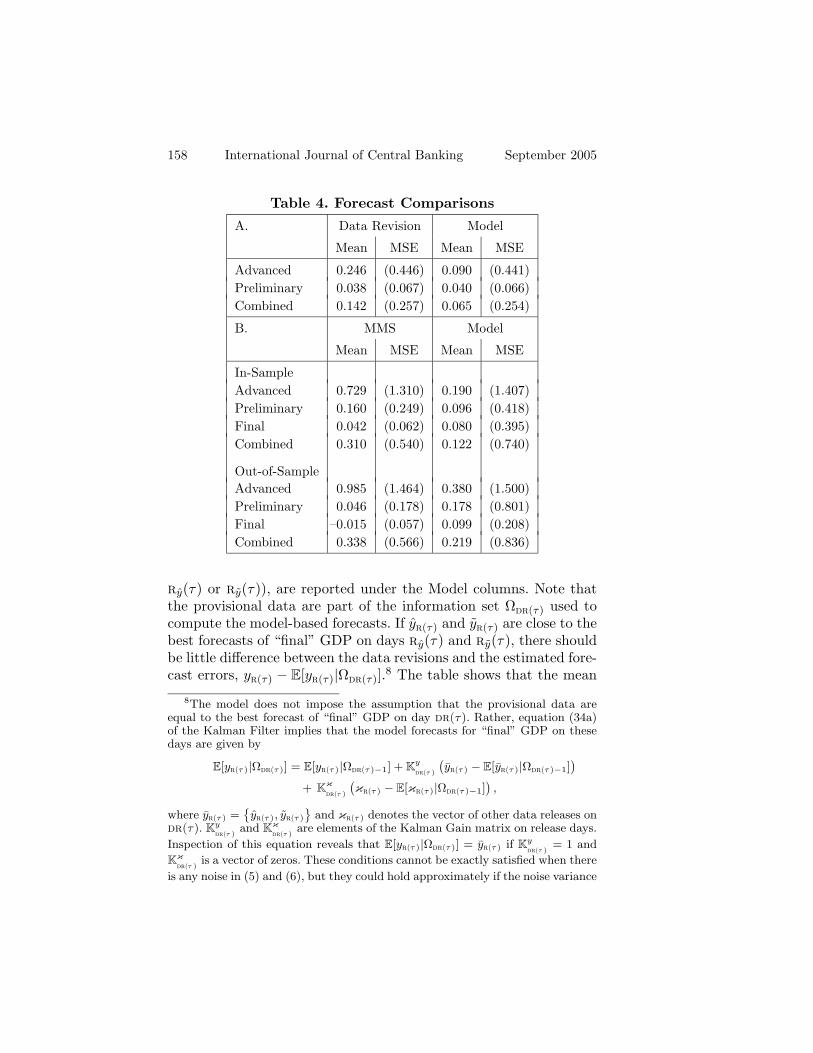
Table 4. Forecast Comparisons

A. Data Revision Model

Mean MSE Mean MSE

Advanced 0.246 (0.446) 0.090 (0.441)Preliminary 0.038 (0.067) 0.040 (0.066)Combined 0.142 (0.257) 0.065 (0.254)

B. MMS Model

Mean MSE Mean MSE

In-SampleAdvanced 0.729 (1.310) 0.190 (1.407)Preliminary 0.160 (0.249) 0.096 (0.418)Final 0.042 (0.062) 0.080 (0.395)Combined 0.310 (0.540) 0.122 (0.740)

Out-of-SampleAdvanced 0.985 (1.464) 0.380 (1.500)Preliminary 0.046 (0.178) 0.178 (0.801)Final –0.015 (0.057) 0.099 (0.208)Combined 0.338 (0.566) 0.219 (0.836)

ry(τ) or ry(τ)), are reported under the Model columns. Note thatthe provisional data are part of the information set Ω

dr(τ) used tocompute the model-based forecasts. If y

r(τ) and yr(τ) are close to the

best forecasts of “final” GDP on days ry(τ) and ry(τ), there shouldbe little difference between the data revisions and the estimated fore-cast errors, y

r(τ) − E[yr(τ)|Ωdr(τ)].8 The table shows that the mean

8The model does not impose the assumption that the provisional data areequal to the best forecast of “final” GDP on day dr(τ). Rather, equation (34a)of the Kalman Filter implies that the model forecasts for “final” GDP on thesedays are given by

E[yr(τ )|Ωdr(τ )] = E[yr(τ )|Ωdr(τ )−1] + Ky

dr(τ )

(yr(τ ) − E[yr(τ )|Ωdr(τ )−1]

)+ K

κ

dr(τ )

(κr(τ ) − E[κr(τ )|Ωdr(τ )−1]

),

where yr(τ ) =yr(τ ), yr(τ )

and κr(τ ) denotes the vector of other data releases on

dr(τ). Kydr(τ )

and Kκ

dr(τ )are elements of the Kalman Gain matrix on release days.

Inspection of this equation reveals that E[yr(τ )|Ωdr(τ )] = yr(τ ) if Kydr(τ )

= 1 and

Kκ

dr(τ )is a vector of zeros. These conditions cannot be exactly satisfied when there

is any noise in (5) and (6), but they could hold approximately if the noise variance


and MSE of revision errors based on the “preliminary” data releasesare comparable to those based on the model forecasts. In the caseof the “advanced” releases, by contrast, the mean revision error isroughly two and one-half times the size of the forecast error. Thisfinding suggests that the “advanced” releases contain some “noise”and do not represent the best forecasts for “final” GDP that can becomputed using publicly available data. It is also consistent with theregression findings reported by Dynan and Elmendorf (2001).

Panel B of table 4 compares the forecasting performance of themodel against the survey responses collected by MMS. On the Fri-day before each scheduled data release, MMS surveys approximatelyforty professional money managers on their estimate for the upcom-ing release. Panel B compares the median estimate from the sur-veys against the real-time estimate of GDP growth implied by themodel on survey days. For example, in the first row under the MMScolumns, I report the mean and MSE for the difference betweenyr(τ), and the median response from the survey conducted on the

last Friday before the “advanced” GDP release on day s(τ). Themean and MSE of the difference between y

r(τ) and the estimate ofE[y

r(τ)|Ωs(τ)] derived from the model are reported under the Modelcolumns. As above, all the survey and model estimates are comparedagainst the value for the “final” GDP release. This means that theforecasting horizon, (i.e., the difference between r(τ) and s(τ)) fallsfrom approximately eleven weeks in the first row, to five weeks in thesecond, and less than one week in the third. The fourth row reportsthe mean and MSE at all three horizons.

The upper portion of panel B compares the survey responsesagainst model-based forecasts computed from parameter estimatesreported in table 2. These estimates are derived from the full datasample and so contain information that was not available to themoney managers at the time they were surveyed. The lower portionof panel B reports on a pseudo out-of-sample comparison. Here themodel-based forecasts are computed from model estimates obtainedfrom the first half of the sample (April 11, 1993–March 31, 1996).These estimates are then used to compute model-based forecasts of“final” GDP on the survey days during the second half of the sample(April 1, 1996–June 30, 1999). The table compares the mean and

is small relative to the variance of other shocks. Under these circumstances, theprovisional data could closely approximate the model’s forecasts for “final” GDP(i.e., E[yr(τ )|Ωdr(τ )] yr(τ )).


MSE of these out-of-sample forecasts against the survey responsesduring this latter period.

The table shows that both the mean and MSE associated withboth the survey and model forecasts fall with the forecasting horizon.In the case of the in-sample statistics, the median survey responseprovides a superior forecast than the model in terms of mean andMSE at short horizons. Both the mean and MSE are smaller forsurvey responses than the model forecasts in the third row. Movingup a row, the evidence is ambiguous. The model produces a smallermean but larger MSE than the median survey. In the first row, thebalance of the evidence favors the model; the MSE is slightly higherbut the mean is much lower than the survey estimates. This generalpattern is repeated in the out-of-sample statistics. The strongest sup-port for the model again comes from a comparison of the survey andmodel forecasts conducted one week before the “advanced” release.In this case, the mean forecast error from the model is approxi-mately 60 percent smaller than the mean survey error. Over shorterforecasting horizons, the survey measures dominate the model-basedforecasts.

Overall, these forecast comparisons provide rather strong sup-port for the model. It is clear that the in-sample comparisons usemodel estimates based in part on information that was not avail-able to the money managers at the time. But it is much less clearwhether this puts the managers at a significant informational dis-advantage. Remember that the money managers had access to pri-vate information and other contemporaneous data that is absentfrom the model. Moreover, we are comparing a model-based forecastagainst the median forecast from a forty-manager survey. In the out-of-sample comparisons, the informational advantage clearly lies withthe managers. Here the model forecasts are based on a true subset ofthe information available to managers, so the median forecast froma forty-manager survey should outperform the model. This is whatwe see when the forecasting horizon is less than five weeks. At longerhorizons, the use of private information imparts less of a forecastingadvantage to money managers.9 In fact, the results suggest that as

9This advantage might be further reduced if each of the model forecasts werecomputed using parameter estimates that utilized all the data available on thesurvey date rather than a single set of estimates using data from the first halfof the sample. A full-blown real-time forecasting exercise of this kind would be


we move the forecasting day back toward the end of quarter τ , boththe in- and out-of-sample model-based forecasts outperform the sur-veys. When the forecasting day is pushed all the way back to theend of the quarter, the model-based forecast gives us the real-timeestimates of GDP growth. Thus, the results in panel B indicatethat real-time estimates derived from the model should be at leastcomparable to private forecasts based on much richer informationsets.

5. Analysis

This section examines the model estimates. First, I consider the re-lation between the real-time estimates and the “final” GDP releases.Next, I compare alternative real-time estimates for the level of GDPand examine the forecasting power of the model. Finally, I study howthe monthly releases are related to changes in GDP at a monthly fre-quency.

5.1 Real-Time Estimates over the Reporting Lag

Figure 2 allows us to examine how the real-time estimates of GDPgrowth change over the reporting lag. The solid line with stars plotsthe “final” GDP growth for quarter τ released on day ry(τ). Theintermittent line plots the real-time estimates of the GDP growthlast month, ∆qx

q(τ)|t, where q(τ) < t ≤ ry(τ) for each quarter. Thevertical dashed portion represents the discontinuity in the series atthe end of each quarter (i.e., on day q(τ)).10 Several features ofthe figure stand out. First, the real-time estimates vary considerablyin the days immediately after the end of the quarter. For example,

computationally demanding because the model would have to be repeatedly esti-mated, but it should also give superior model-based forecasts. For this reason, theout-of-sample exercise undertaken here probably understates the true real-timeforecasting potential of the model.

10In cases where the reporting lag is less than one quarter, the discontinuityoccurs (a couple of days) after ry(τ), so the end of each solid segment meets theturning point “x” identifying the “final” GDP release. When the reporting lagis longer than one quarter, there is a horizontal gap between the end of a solidsegment and the next turning point “x” equal to ry(τ)−q(τ + 1) days.


Figure 2. Real-Time Estimates of Quarterly GDP Growth

Note: The intermittent solid line is the real-time estimate of quarterly GDPgrowth, ∆qxq(τ)|t, where Q(τ) < t ≤ |Ry(τ), and the solid line with starsis the “final” release for GDP, yr(τ).

at the end of 1994, the real-time estimates of GDP growth in thefourth quarter change from approximately 1.25 percent to 2.25 per-cent and then to 1.5 percent in the space of a few days. Second,in many cases there is very little difference between the value for“final” GDP and the real-time estimate immediately prior to therelease (i.e., y

r(τ) ∆qxq(τ)|r(τ)−1). In these cases, the “final” re-

lease contains no new information about GDP growth that was notalready inferred from earlier data releases. In cases where the “fi-nal” release contains significant new information, the intermittent-line plot “jumps” to meet the solid-line-with-stars plot on the releaseday.

Figure 3 provides further information on the relation betweenthe real-time estimates and the “final” data releases. Here I plotthe variance of ∆qx

q(τ) conditioned on information available over


Figure 3. Relation between Real-Time Estimates and the“Final” Data Releases

Note: The solid line is the sample average of V(∆qxq(τ)|Ωq(τ)+i) for 0 < i ≤ry(τ)−q(τ), and the dashed lines denote the 95 percent confidence band.The horizontal axis marks the number of days i past the end of quarterq(τ).

the reporting lag: V(∆qxq(τ)|Ωq(τ)+i) for 0 < i ≤ ry(τ)−q(τ).

Estimates of this variance are identified as the second diagonal el-ement in St+1|t obtained from the Kalman Filter evaluated at themaximum likelihood estimates. Figure 3 plots the sample average ofV(∆qx

q(τ)|Ωq(τ)+i) together with a 95 percent confidence band. Al-though the path for the conditional variance varies somewhat fromquarter to quarter, the narrow confidence band shows that the aver-age pattern displayed in the figure is in fact quite representative ofthe variance path seen throughout the sample.

Figure 3 clearly shows how the flow of data releases during the re-porting lag provides information on ∆qx

q(τ). In the first twenty daysor so, the variance falls by approximately 25 percent as informationfrom the monthly releases provides information on the behavior of


GDP during the previous month (month 3 of quarter τ). The vari-ance then falls significantly following the “advanced” GDP release.The timing of this release occurs between nineteen and twenty-threeworking days after the end of the quarter, so the averaged variancepath displayed by the figure spreads the fall across these days. There-after, the variance falls very little until the end of the reporting lagwhen the “final” value for GDP growth is released.11 This patternindicates that the “preliminary” GDP release provides little newinformation about GDP growth beyond that contained in the “ad-vanced” GDP release and the monthly data. The figure also showsthat most of the uncertainty concerning GDP growth in the lastquarter is resolved well before the day when the “final” data is re-leased.

5.2 Real-Time Estimates of GDP and GDP Growth

Figure 4 compares the real-time estimates of log GDP against thevalues implied by the “final” GDP growth releases. The solid lineplots the values of x

q(τ)|t computed from (43):

xq(τ)|t = E[xt|Ωt] +

q(τ)−t∑h=1

E[∆xt+h|Ωt]. (43)

Recall that xq(τ) represents log GDP for quarter τ , so x

q(τ)|t includesforecasts for ∆xt+h over the remaining days in the quarter whent < q(τ). To assess the importance of the forecast terms, figure 4also plots E[xt|Ωt] as a dashed line. This series represents a naivereal-time estimate of GDP since it assumes E[∆xt+h|Ωt] = 0 for1 ≤ h ≤q(τ) − t. The dash-dot line in the figure plots the cumulantof the “final” GDP releases

∑τi=1 y

r(i) with a lead of sixty days. Thisplot represents an ex-post estimate of log GDP based on the “final”data releases. The vertical steps identify the values for “final” GDPgrowth sixty days before the actual release day.

11Although the variance falls immediately to zero on the day of the release,the averaged variance falls to zero over several days in the figure because thereporting lag varies from fifty-eight to sixty-five workdays in the sample.


Figure 4. Real-Time Estimates of Log GDP and “Final”GDP Releases

Note: The solid line is the real-time estimate of log GDP, xq(τ)|t, the dashedline shows E[xt|Ωt], and the dash-dot line is the cumulant of “final” GDPreleases.

Figure 4 displays three notable features. First, both sets of thereal-time estimates display a much greater degree of volatility thanthe cumulant series. This volatility reflects how inferences about cur-rent GDP change as information arrives in the form of monthly datareleases during the current quarter and GDP releases referring togrowth in the previous quarter. The second noteworthy feature con-cerns the relation between the real-time estimates. The vertical dif-ference between the solid-line plots and the dashed-line plots repre-sents the contribution of the ∆xt+h forecasts to x

q(τ)|t. As the figureshows, these forecasts contributed significantly to the real-time es-timates in 1996 and 1997, pushing the real-time estimates of x

q(τ)

well below the value for E[xt|Ωt]. The third noteworthy feature of thefigure concerns the vertical gap between the solid-line and dash-dot


line plots. This represents the difference between the real-time esti-mates and an ex-post estimate of log GDP based on the “final” GDPreleases. This gap should be insignificant if the current level of GDPcould be precisely inferred from contemporaneously available datareleases. Figure 3 shows this to be the case during the third andfourth quarters of 1995. During many other periods, the real-timeestimates were much less precise.

5.3 Forecasting GDP Growth

The model estimates in table 2 show that all of the φi coefficientsin the daily growth process are statistically significant. I now ex-amine their implications for forecasting GDP growth. Consider thedifference between the real-time estimates of xt+m and xt+n basedon information available on days t + m and t + n, where m > n:

xt+m|t+m − xt+n|t+n =t+m∑

h=t+n+1

E [∆xh|Ωt] +(xt+m|t+m − xt+m|t

)

−(xt+n|t+n − xt+n|t

). (49)

This equation decomposes the difference in real-time estimates of xt

into forecasts for ∆xt over the forecast horizon between t + n andt+m, the revision in the estimates of xt+m between t and t+m andxt+n between t and t + n.

Since both revision terms are uncorrelated with elements of Ωt,we can use (49) to examine how the predictability of ∆xt impliedby the model estimates translates into predictability for changes inxt|t. In particular, after multiplying both sides of (49) by xt+m|t+m−xt+n|t+n and taking expectations, we obtain

R2 (m, n) =

∑t+mh=t+n+1 CV

(E [∆xh|Ωt] , xt+m|t+m − xt+n|t+n

)V

(xt+m|t+m − xt+n|t+n

) .

This statistic measures the contribution of ∆xt forecasts to the vari-ance of xt+m|t+m − xt+n|t+n. If most of the volatility in xt+m|t+m −xt+n|t+n is due to the arrival of new information between t and t+m

(i.e., via the revision terms in [49]), the R2 (m, n) statistic should

be close to zero. Alternatively, if the daily growth process is highly


Table 5. Forecasting Real-Time GDP

m R2(m,n) (std.)

Monthly (n = m − 20)

20 0.196 (0.015)40 0.186 (0.014)60 0.180 (0.013)80 0.163 (0.013)

100 0.138 (0.012)120 0.125 (0.011)140 0.097 (0.010)160 0.061 (0.007)180 0.032 (0.006)200 0.035 (0.006)220 0.027 (0.006)240 0.005 (0.006)

Quarterly (n = m − 60)

60 0.144 (0.008)120 0.079 (0.006)180 0.031 (0.003)240 0.006 (0.002)

Note: The table reports estimates ofR2(m,m − 20) computed as the slopecoefficient δm from the regression∑t+m

h=t+m−19 E [∆xh|Ωt] = δm(xt+m|t+m−xt+m−20|t+m−20) + ξt+m computed in dailydata from the maximum likelihood esti-mates of xt+m|t+m − xt+m−20|t+m−20 andE [∆xh|Ωt] . OLS standard errors are reportedin the right-hand column.

forecastable, much less of the volatility in xt+m|t+m − xt+n|t+n willbe attributable to news, and the R

2 (m, n) statistic will be positive.Table 5 reports estimates for R

2(m, n) for various forecastinghorizons. The estimates are computed as the slope coefficient in theregression of

∑t+mh=t+n+1 E [∆xh|Ωt] on xt+m|t+m − xt+n|t+n in daily

data. The table also reports OLS (ordinary least squares) standard


errors in parentheses.12 The upper panel shows how predictable themonthly changes in the real-time estimates of xt are for horizonsm of 20 to 240 days. The estimated process for ∆xt implies a rea-sonable high degree of predictability: the R

2 estimates fall from ap-proximately 20 to 10 percent as the horizon rises from 20 to 140workdays. Estimates of R

2(m, n) for quarterly changes in the real-time estimates are reported in the lower panel of the table. These aresomewhat smaller, but again clearly indicate the presence of somepredictability.

The results in table 5 relate to the change in the real-time es-timates of xt rather than GDP growth. Recall from (43) that thereal-time estimate of log GDP on day t in quarter τ is x

q(τ t)|t =

E[xt|Ωt] +∑

q(τ t)h=t+1 E[∆xh|Ωt], so the growth in quarterly GDP be-

tween quarters τ and τ +1 based on the real-time estimates availableat t + m and t + n (where t + n < q(τ) < t + m < q(τ + 1)) is

xq(τ+1)|t+m − x

q(τ)|t+n =(xt+m|t+m − xt+n|t+n

)

+q(τ+1)∑

h=t+m+1

E[∆xh|Ωt+m]

−q(τ)∑

h=t+n+1

E[∆xh|Ωt+n]. (50)

This equation shows that changes in the real-time estimates of xt

are only one component of the estimated quarterly growth in GDP.Moreover, since the second and third terms on the right-hand sideof (50) will generally be correlated with the first term, the resultsin table 5 may be an unreliable guide to the predictability of GDPgrowth.

We can examine the predictability of GDP growth by combining(49) and (50) to give

xq(τ+1)|t+m − x

q(τ)|t+n = E[xq(τ+1) − x

q(τ)+1|Ωt] + ςt+m,

12These statistics only approximate to the true standard errors for two reasons.First, the regressor is computed from the maximum likelihood estimates and socontains some sampling errors. Second, there is no correction for the movingaverage process induced by the overlapping forecast horizons in the regressionresiduals.


Figure 5. Real-Time Estimates of Quarterly GDP Growth

Note: The solid line is the real-time estimate of quarterly GDP growth,xq(τ+1)|t+60 − xq(τ)|t, and the dashed line is the forecast, E[xq(τ+1) −xq(τ)|Ωt].

where ςt+m is an error term that depends on news that arrives be-tween t and t + m. This equation shows that GDP growth shouldbe predictable in the model because the process for ∆xt impliesthat E[x

q(τ+1) − xq(τ)+1|Ωt] changes over the sample. Figure 5 plots

the estimates of E[xq(τ+1) − x

q(τ)+1|Ωt] and xq(τ+1)|t+m − x

q(τ)|t+n

for m = 60 and n = 0. Clearly, news contributes significantlyto the volatility of GDP growth since the E[x

q(τ+1) − xq(τ)+1|Ωt]

series is much less volatile than xq(τ+1)|t+m − x

q(τ)|t+n. In fact,only 6 percent of the variance in x

q(τ+1)|t+m − xq(τ)|t+n can be at-

tributable to E[xq(τ+1) − x

q(τ)+1|Ωt] over the sample. While this


implies a rather modest degree of predictability, close inspection offigure 5 suggests that predicting the future direction of GDP growthmay be a little more successful. Indeed, the model estimates ofE[x

q(τ+1)−xq(τ)+1|Ωt] correctly predict the direction of GDP growth

59 percent of the time.For perspective on these forecasting results, I also estimated an

AR(2) model for quarterly GDP growth using the sequence of “fi-nal” GDP releases. This model provides a simple time-series forecastfor GDP growth (approximately) one quarter ahead, based on thetwo most recent releases. In contrast to the results presented above,estimates of the AR(2) model do not indicate that quarterly GDPgrowth is at all predictable: the coefficients are small and statis-tically insignificant, and the R2 statistic is only 3 percent. Theseresults are hardly surprising. Remember that the sample mean wasremoved from all the GDP growth releases, so we are attemptingto forecast future deviations in GDP growth. Figure 2 shows thatthese deviations display little serial correlation. Thus, it is not sur-prising that the history of GDP releases has little forecasting power.These observations also point to the significance of the forecastingresults displayed in table 5 and figure 5. In particular, they show thatmonthly data releases contain information that is useful for both es-timating the current state of the GDP and for forecasting its futurepath. This aspect of the model ties in with recent research that har-nesses the information in a large number of indicators for forecasting(see, for example, Stock and Watson 2002). The results from thesestudies suggest that the real-time forecasting performance of thismodel may be further enhanced by addition of other macroeconomicand financial indicators.

5.4 Monthly Estimates of GDP Growth

One of the unique features of the model is its ability to provide uswith high-frequency estimates of log GDP and GDP growth. I nowexamine how the monthly data releases relate to the changing real-time estimates of log GDP. My aim is to provide a simple descriptionof the complex inference problem solved by the model regarding thecurrent state of GDP.

Let t and t + 20 be workdays in quarters τ0 and τ1 with t ≤q(τ0) and t + 20 ≤ q(τ1). (Note that τ0 and τ1 can refer to the


same quarter.) I consider two regression models. The first relates themonthly change in the real-time estimates of log GDP to all eighteenmonthly releases:

xq(τ1)|t+20 − x

q(τ0)|t =18∑i=1

ai(rit+20 − ri

t) + ζt+20, (51)

where rit denotes the last value released for series i on day t. Thus,

the value of rit remains the same from day to day unless t is the

day on which a data release for series i takes place. This means thatrit+20−ri

t identifies the change in the latest value for series i releasedduring the twenty workdays ending on t + 20. The second modelrelates the change in the real-time estimates to each monthly releaseseparately:

xq(τ1)|t+20 − x

q(τ0)|t = bi(rit+20 − ri

t) + ζt+20, (52)

for i = 1, 2, . . . , 18. Notice that the regressors in both models areavailable on a daily basis. Estimates of the ai and bi coefficients there-fore summarize how the complex inference imbedded in the modelrelates to observable changes in the information set comprised ofmonthly data releases.

Table 6 reports the estimates of equations (51) and (52). Theleft-hand columns show that the ai estimates are statistically sig-nificant for data on nonfarm payroll employment, retail sales, in-dustrial production, personal consumption, factory orders, the tradebalance, the index of consumer confidence, and housing starts. Eachof these data releases provides significant incremental informationabout the change in the real-time estimates. The eighteen monthlyreleases account for approximately 57 percent of the variance inx

q(τ1)|t+20 − xq(τ0)|t. This means that more than 40 percent of the

variation in the real-time estimates is not captured by the simplelinear specification. The right-hand columns report the results fromestimating equation (52). The most noteworthy aspects of these es-timates can be seen for i = 1, 2, 3. Changes in both nonfarm payrollemployment and retail sales appear strongly linked to changes inthe real-time estimates. Based on the R2 statistics (in the right-hand column), these variables account for 23 and 19 percent of thevariance in the real-time estimates. The results for i = 3 providesome justification for the frequent use of industrial production as a


Table 6. Monthly Indicator EstimatesData Release ai std(ai ) bi std(bi ) R2

1 Nonfarm Payroll Employment 0.224∗ (0.033) 0.330∗ (0.050) 0.233

2 Retail Sales 0.520∗ (0.074) 0.838∗ (0.099) 0.186

3 Industrial Production 0.745∗ (0.116) 1.047∗ (0.142) 0.233

4 Capacity Utilization –0.006 (0.034) 0.066 (0.057) 0.010

5 Personal Income –0.110 (0.132) 0.163 (0.224) 0.003

6 Consumer Credit 0.001 (0.012) –0.002 (0.019) 0.000

7 Personal Consumption 0.377∗ (0.182) 0.603∗ (0.277) 0.033

Expenditures

8 New Home Sales 0.016 (0.069) 0.181∗ (0.088) 0.039

9 Durable Goods Orders 0.013 (0.021) 0.064∗ (0.027) 0.030

10 Construction Spending –0.050 (0.051) –0.102 (0.060) 0.015

11 Factory Orders 0.097∗ (0.038) 0.160∗ (0.043) 0.066

12 Business Inventories –0.013 (0.152) 0.289 (0.247) 0.008

13 Government Budget Deficit –0.008 (0.011) –0.017 (0.016) 0.005

14 Trade Balance –0.071∗ (0.021) –0.068∗ (0.030) 0.042

15 Consumer Confidence Index 0.068∗ (0.028) 0.060 (0.037) 0.021

16 NAPM Index –0.001 (0.145) 0.514∗ (0.216) 0.046

17 Housing Starts –1.330∗ (0.421) 0.705 (0.546) 0.012

18 Index of Leading Indicators 0.164 (0.179) 0.476∗ (0.199) 0.038

Note: The table reports the OLS estimates of ai and bi from equations (51) and (52).Both equations are estimated at the daily frequency, and the standard errors arecorrected for the moving average (19) process induced by the overlapping data. Theright-hand column reports the R2 statistic from estimating equation (52). ∗denotessignificance at the 5 percent level.

monthly proxy for GDP growth. The estimate for b3 indicates thatthe real-time estimates of log GDP change approximately one-for-one with change in industrial production between releases. Notice,however, that the R2 statistic is only 0.233. Industrial productiondoes not account for most of the variance in the real-time estimates.

6. Conclusion

In this paper, I have presented a method for estimating the currentstate of the economy on a continual basis using the flow of infor-mation from a wide range of macroeconomic data releases. Thesereal-time estimates were computed from an econometric model thatallows for variable reporting lags, temporal aggregation, and othercomplications that characterize the daily flow of macroeconomic


information. The model can be applied to find real-time estimates ofGDP, inflation, unemployment, or any other macroeconomic variableof interest.

In this paper, I focused on the problem of estimating GDP inreal time. This application of the estimation procedure should beof particular interest to policymakers concerned with the lack oftimely information about economy-wide real activity. The real-timeestimates I calculate have several noteworthy features: First, the es-timates of log GDP display a good deal of high-frequency volatility.This volatility reflects how inferences about current GDP changeas information arrives in the form of monthly data releases duringthe quarter. Second, the gaps between the real-time estimates andex-post GDP data are on occasion both persistent and significant.These findings suggest that the ex-post data should not be viewedas a close approximation to what was known at the time. Third, themodel estimates reveal that the monthly data releases contain infor-mation that is useful for forecasting the future path of GDP. Finally,my comparison of the real-time estimates with the monthly dataseries shows that standard proxies for real activity at the monthlyfrequency capture only a fraction of the variance in the real-timeestimates.

These findings give but a flavor of the possible uses for real-time estimates. One obvious topic for the future concerns the abilityof the real-time estimates and forecasts to identify turning points inthe business cycle. This issue could be readily addressed if the modelwere reestimated over a much longer time span than was undertakenhere. The use of real-time estimates may also bring new perspectiveto the link between asset prices and macroeconomic fundamentals.Evans and Lyons (2004b) use the methods described here to con-struct real-time estimates for GDP, inflation, and money suppliesfor the United States and Germany. With the aid of these estimates,they then show that foreign exchange transactions contain significantinformation about the future path of fundamentals. Since transactionflows also exert a very strong influence on exchange rate dynamicsin the short run, this finding points to a much stronger link betweenfundamentals and exchange rates than previous research has uncov-ered. It remains to be seen whether the use of real-time estimateswill similarly illuminate the links between macrofundamentals andother asset prices.


References

Andersen, Torben G., Tim Bollerslev, Francis Diebold, and ClaraVega. 2003. “Micro Effect of Macro Announcements: Real-TimePrice Discovery in Foreign Exchange.” American Economic Re-view 93 (1): 38–62.

Balduzzi, Pierluigi, Edwin J. Elton, and T. Clifton Green. 2001.“Economic News and Bond Prices: Evidence from the U.S. Treas-ury Market.” Journal of Financial and Quantitative Analysis 36(4): 523–43.

Carson, Carol S. 1987. “GNP: An Overview of Source Data andEstimation Methods.” Survey of Current Business 67 (7): 103–26.

Chow, Gregory, and An-loh Lin. 1971. “Best Linear Unbiased Inter-polation, Distribution, and Extrapolation of Time Series by Re-lated Time Series.” Review of Economics and Statistics 53:372–75.

Croushore, Dean, and Tom Stark. 1999. “A Real-Time Data Set forMacroeconomists.” Working Paper 99-4, Federal Reserve Bankof Philadelphia (June).

———. 2001. “A Real-Time Data Set for Macroeconomists.” Journalof Econometrics 105 (November): 111–30.

Dynan, Karen E., and Douglas W. Elmendorf. 2001. “Do ProvisionalEstimates of Output Miss Economic Turning Points?” Mimeo,Federal Reserve Board.

Evans, Martin D.D., and Richard K. Lyons. 2004a. “A New MicroModel of Exchange Rate Dynamics.” NBER Working Paper No.10379 (March).

———. 2004b. “Exchange Rate Fundamentals and Order Flow.”Mimeo (March). Available at www.georgetown.edu/faculty/evansm1/wpapers files/flowsandfundamentalsv8.pdf.

Faust, Jon, John Rogers, and Jonathan Wright. 2000. “News andNoise in G-7 GDP Announcements.” Federal Reserve Board In-ternational Finance Discussion Paper No. 2000-690.


Hamilton, James D. 1994. Time Series Analysis. Princeton, NJ:Princeton University Press.

Harvey, Andrew C. 1989. Forecasting Structural Time Series Modelsand the Kalman Filter. Cambridge: Cambridge University Press.

Kitchen, John, and Ralph M. Monaco. 2003. “Real-Time Forecastingin Practice: The U.S. Treasury Staff’s Real-Time GDP ForecastSystem.” Business Economics (October): 10–19.

Liu, Hong, and Stephen G. Hall. 2000. “Creating High FrequencyNational Accounts with State Space Modelling: A Monte CarloExperiment.” Mimeo, Imperial College, London, United King-dom.

Mankiw, N. Gregory, and Matthew D. Shapiro. 1986. “News or Noise:An Analysis of GNP Revisions.” Survey of Current Business 66(5): 20–5.

Mariano, Roberto, and Yasutomo Murasawa. 2003. “A New Coinci-dent Index of Business Cycles Based on Monthly and QuarterlySeries.” Journal of Applied Econometrics 18:427–43.

Orphanides, Athanasios. 2001. “Monetary Policy Rules Based onReal-Time Data.” American Economic Review 91 (4): 964–85.

Robertson, John C., and Ellis W. Tallman. 1999. “Vector Autoregres-sions: Forecasting and Reality.” Federal Reserve Bank of AtlantaEconomic Review 84 (1): 4–18.

Seskin, Eugene P., and Robert P. Parker. 1998. “A Guide to theNIPA’s.” Survey of Current Business 78 (3): 26–68.

Stock, James H., and Mark W. Watson. 2002. “Macroeconomic Fore-casting Using Diffusion Indexes.” Journal of Business and Eco-nomic Statistics 20 (2): 147–62.

Urich, Thomas J., and Paul Watchel. 1984. “The Effects of Inflationand Money Supply Announcements on Interest Rates.” Journalof Finance 39 (4): 1177–88.

WhereAreWeNow? Real-Time Estimates of the Macroeconomy

Documents

Transcript of WhereAreWeNow? Real-Time Estimates of the Macroeconomy