Wheeler, W.C. 2006.

Dynamic homology and the likelihood criterion

Ward C. Wheeler

Division of Invertebrate Zoology, American Museum of Natural History, Central Park West at 79th Street, New York, NY 10024-5192, USA

Accepted 6 December 2005

Abstract

The use of likelihood as an optimality criterion is explored in the context of dynamic homology. Simple models and proceduresare described to allow the analysis of large variable length sequence data sets, alone and in combination with qualitative information(such as morphology). Several approaches are discussed that have different likelihood interpretations in terms of maximumparsimony likelihood and maximum average likelihood. Implementation is discussed and an example in arthropod systematicspresented. Topological congruence comparisons with parsimony are made.� The Willi Hennig Society 2006.

Dynamic homology

Nucleic acid sequence data do not present themselvesin neat packages. Nucleotide homologies are topologyspecific and identified by optimization processes thatdetermine nucleotide correspondence and transforma-tion via a specific criterion. This is the concept ofdynamic homology (Wheeler, 2001; Wheeler et al.,2005b). Methods have been proposed to apply thismanner of thinking using parsimony as an optimalitycriterion (Wheeler, 1996, 1999a, 2003a,b) which havetheir roots with Sankoff (1975), but less work has beendone to explore the use of likelihood as an alternateinterpretive framework.

Several methods for analyzing unaligned sequencedata using likelihood as an optimality criterion in adynamic homology framework are proposed here. Thesetechniques are optimization methods in the sense ofWheeler (2005) in that they do not rely on a priorimultiple alignments (although they may generate them aposteriori), but analyze variation directly, yielding opti-mal—in this case likely—cladograms. To accomplish

this, models that can accommodate insertion-deletioninformation are required.

Likelihood alignment models

Although there exist a large diversity of nucleotidesubstitution models, there are far fewer which model theinsertion-deletion process. The most prominent of thesemodels is that of Thorne et al. (1991) (TKF) for thestatistical alignment of two sequences. TKF allows fortransitions among nucleotides, as well as their insertionand deletion through a birth ⁄death process of gaps. Themodel yields the probability of one sequence evolvinginto another over a given time interval, and wasexpanded in Thorne et al. (1992) to include affine gapsand rate heterogeneity. Fleissner et al. (2005) used thelatter in their multiple-alignment approach, andRedelings and Suchard (2005) added additionalgeneralizations for their Bayesian approach.

An important advance of the TKF model overprevious attempts (e.g., Bishop and Thompson, 1986)is that the total probability of transformation betweensequences is the sum of all possible alignments betweenthe sequences (and there may be many of them;Slowinski, 1998). The unique alignment that is usuallyE-mail address: [email protected]

� The Willi Hennig Society 2006

Cladistics

www.blackwell-synergy.com

Cladistics 22 (2006) 157–170

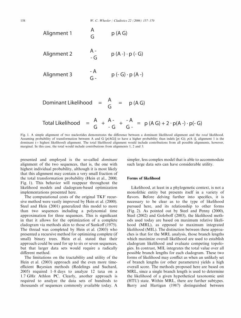
presented and employed is the so-called dominantalignment of the two sequences, that is, the one withhighest individual probability, although it is most likelythat this alignment may contain a very small fraction ofthe total transformation probability (Hein et al., 2000;Fig. 1). This behavior will reappear throughout thelikelihood models and cladogram-based optimizationimplementations presented here.

The computational costs of the original TKF recur-sive method were vastly improved by Hein et al. (2000).Steel and Hein (2001) generalized this model to morethan two sequences including a polynomial timeapproximation for three sequences. This is significantin that it allows for the optimization of a completecladogram via methods akin to those of Sankoff (1975).The thread was completed by Hein et al. (2003) whopresented a recursive method for optimizing complete (ifsmall) binary trees. Hein et al. stated that theirapproach could be used for up to six or seven sequences,but that larger data sets would require a radicallydifferent method.

The limitations on the tractability and utility of theHein et al. (2003) approach and the even more time-efficient Bayesian methods (Redelings and Suchard,2005) required 1–8 days to analyze 12 taxa on a1.7 GHz Athlon PC. Clearly, another approach isrequired to analyze the data sets of hundreds tothousands of sequences commonly available today. A

simpler, less complex model that is able to accommodatesuch large data sets can have considerable utility.

Forms of likelihood

Likelihood, at least in a phylogenetic context, is not amonolithic entity but presents itself in a variety offlavors. Before delving further into specifics, it isnecessary to be clear as to the type of likelihoodpursued here, and its relationship to other forms(Fig. 2). As pointed out by Steel and Penny (2000),Steel (2002) and Goloboff (2003), the likelihood meth-ods used today are based on maximum relative likeli-hood (MRL), as opposed to maximum integratedlikelihood (MIL). The distinction between these approa-ches is that for the MRL analysis, those branch lengthswhich maximize overall likelihood are used to establishcladogram likelihood and evaluate competing topolo-gies. In contrast, MIL integrates the total value over allpossible branch lengths for each cladogram. These twoforms of likelihood may conflict as when an unlikely setof branch lengths (or other parameters) yields a highoverall score. The methods proposed here are based onMRL, since a single branch length is used to determinethe likelihood of a given hypothetical taxonomic unit(HTU) state. Within MRL, there are further subtypes.Barry and Hartigan (1987) distinguished between

Fig. 1. A simple alignment of two nucleotides demonstrates the difference between a dominant likelihood alignment and the total likelihood.Assuming probability of transformation between A and G [p(AG)] to have a higher probability than indels [p(–G); p(A–)], alignment 1 is thedominant (¼ highest likelihood) alignment. The total likelihood alignment would include contributions from all possible alignments, however,marginal. In this case, the total would include contributions from alignments 1, 2 and 3.

158 W. C. Wheeler / Cladistics 22 (2006) 157–170

maximum average likelihood (MAL) and maximumparsimony likelihood (MPL). The MAL approach inessence averages over all possible internal nodal states(HTU assignments), whereas MPL assigns a single stateor sequence that maximizes the likelihood. MPL meth-ods have the benefit of being much simpler to compute,since only a single (but hopefully highly likely) scenariois required, as opposed to the potentially large universeof solutions. Both the MAL and MPL methods arepresented here. A third approach is the evolutionarypath method of Farris (1973). In this form of MRL, theactual sequence of intermediate states is chosen tomaximize likelihood. This yields precisely the sameresult as parsimony, even under variations in mutation

rates and branch lengths (Farris, 1973). The evolution-ary path likelihood is not implemented by any of themethods proposed here.

A simple likelihood model

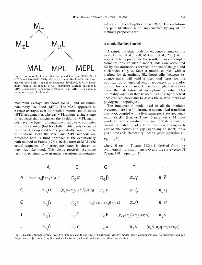
A simple five-state model of sequence change can beused (Durbin et al., 1998; McGuire et al., 2001) at thevery least to approximate the results of more complexformalizations. In such a model, indels are accountedfor by transformations between the state of the gap andnucleotides (Fig. 3). Such a model, coupled with amethod for determining likelihood edits between se-quence pairs, will yield a likelihood basis for theoptimization of unequal length sequences on a clado-gram. This type of model may be rough, but it doesallow the calculation of an optimality value. Thisoptimality value can then be used to choose hypotheticalancestral sequences and to assess the relative merits ofphylogenetic topologies.

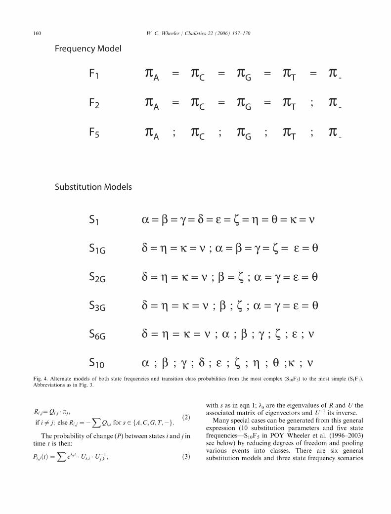
The fundamental model used in all the methodspresented here is a 10-parameter symmetrical transitionmatrix Q, coupled with a five-parameter state frequencyvector (S10F5) (Fig. 4). These 15 parameters (14 inde-pendent since the p-values must sum to 1) determine theoverall probabilities of a transformation among eachpair of nucleotides and gap (signifying an indel) for agiven time t via elementary linear algebra (equation 1):

P ðtÞ ¼ eRt; ð1Þ

where R (as in Tavare, 1986) is derived from thesymmetrical transition matrix Q and the state vector P(Yang, 1994; equation 2).

Fig. 3. General, though symmetrical, five state nucleotide and gap (�–�) stationary Markov model. The p components refer to nucleotide and gapfrequencies; a, b, c, d, e, f, g, h, j and m refer to the nucleotide and indel transition probabilities.

Fig. 2. Forms of likelihood after Barry and Hartigan (1987), Steel(2002) and Goloboff (2003). ML ¼ maximum likelihood in the mostgeneral sense, MIL ¼ maximum integrated likelihood, MRL ¼ maxi-mum relative likelihood, MAL ¼ maximum average likelihood,MPL ¼ maximum parsimony likelihood, and MEPL ¼ maximumevolutionary path likelihood.

159W. C. Wheeler / Cladistics 22 (2006) 157–170

Ri;j¼Qi;j � pj;if i 6¼ j; else Ri;j ¼�

XQi;s for s 2 fA;C;G;T ;�g:

ð2Þ

The probability of change (P) between states i and j intime t is then:

Pi;jðtÞ ¼X

ekst � Us;i � U�1j;k ; ð3Þ

with s as in eqn 1; ks are the eigenvalues of R and U theassociated matrix of eigenvectors and U)1 its inverse.

Many special cases can be generated from this generalexpression (10 substitution parameters and five statefrequencies—S10F5 in POY Wheeler et al. (1996–2003)see below) by reducing degrees of freedom and poolingvarious events into classes. There are six generalsubstitution models and three state frequency scenarios

Fig. 4. Alternate models of both state frequencies and transition class probabilities from the most complex (S10F5) to the most simple (S1F1).Abbreviations as in Fig. 3.


for 18 model combinations from a InDel-Jukes-Cantor(Jukes-Cantor + Gaps; S1F1) where all transitions andall state frequencies are equal, to the 14 parameterInDel-GTR (the 11 parameter would also be a GTRmodel) (GTR + Gaps; Fig. 5). Furthermore, thesemodel parameters can be determined individually fordifferent fragments of DNA and even for the individualbranches of the topologies examined during a search. Ingeneral, investigators seem to prefer homogeneous indelprobabilities (or costs) such that indels of A, C, G or Tdo not differ. For this reason, the S1G, S2G, S3G and S6Gmodels restrict indels to a single probability. The S10model removes this restriction. Comparison of thebehavior of these models would allow a test of theassumption of indel homogeneity.

Following parsimony-based techniques, there are twoclasses of methods presented here to employ likelihoodas a criterion for dynamic homology-based analysis:estimation and search methods (sensu Wheeler, 2005).The estimation methods are heuristics that seek to createlikely HTU sequences such that the overall cladogramlikelihood is maximized. Likelihood versions of DirectOptimization (Wheeler, 1996) and Iterative-Pass opti-mization (Wheeler, 2003a) fall into this camp. In theirfocus on likely HTUs, these methods are MPL methodsin the sense of Barry and Hartigan (1987), though thereare elements that can be described as MAL. The search-based methods, Fixed-State (Wheeler, 1999a) andSearch-Based Optimization (Wheeler, 2003b), can beimplemented as either MPL or MAL methods and bothare discussed here. All of these methods are heuristic

cladogram optimization procedures of the same basicmodel. The problems of cladogram search and tree-alignment (Wang and Jiang, 1994) are known to be NP-complete and none of these methods (other thanexhaustive Search-Based Optimization) guarantees anexact solution for more than two sequences.

Direct optimization (DO)

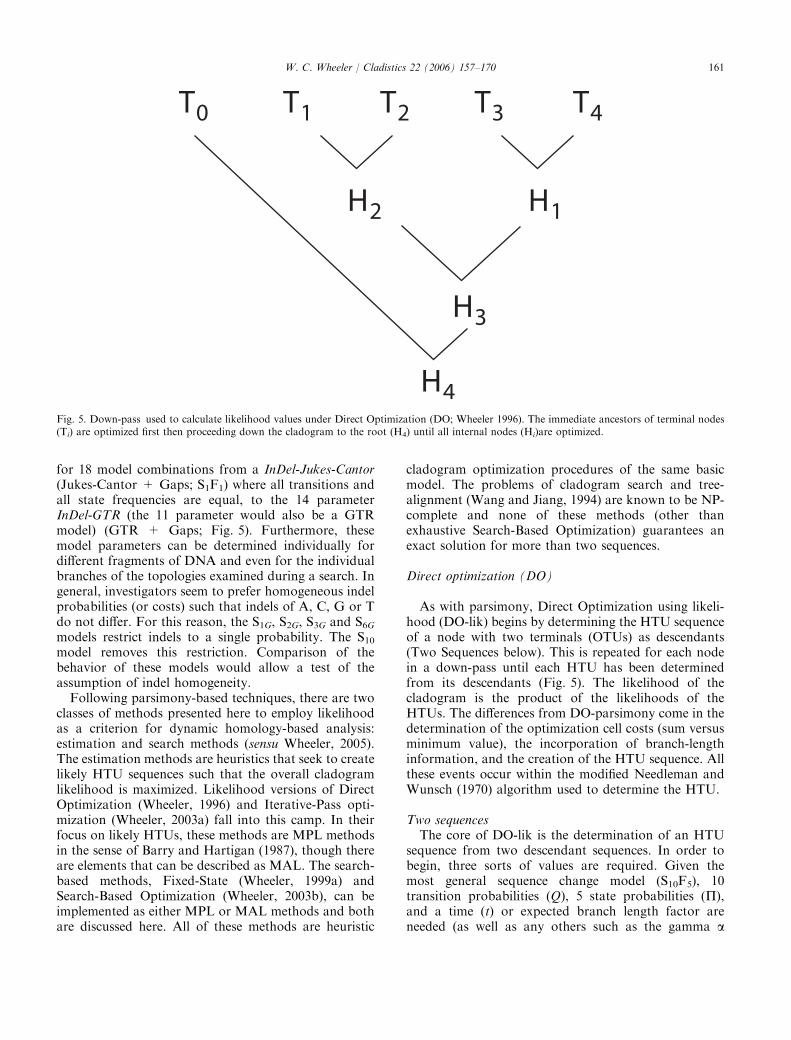
As with parsimony, Direct Optimization using likeli-hood (DO-lik) begins by determining the HTU sequenceof a node with two terminals (OTUs) as descendants(Two Sequences below). This is repeated for each nodein a down-pass until each HTU has been determinedfrom its descendants (Fig. 5). The likelihood of thecladogram is the product of the likelihoods of theHTUs. The differences from DO-parsimony come in thedetermination of the optimization cell costs (sum versusminimum value), the incorporation of branch-lengthinformation, and the creation of the HTU sequence. Allthese events occur within the modified Needleman andWunsch (1970) algorithm used to determine the HTU.

Two sequencesThe core of DO-lik is the determination of an HTU

sequence from two descendant sequences. In order tobegin, three sorts of values are required. Given themost general sequence change model (S10F5), 10transition probabilities (Q), 5 state probabilities (P),and a time (t) or expected branch length factor areneeded (as well as any others such as the gamma a

Fig. 5. Down-pass used to calculate likelihood values under Direct Optimization (DO; Wheeler 1996). The immediate ancestors of terminal nodes(Ti) are optimized first then proceeding down the cladogram to the root (H4) until all internal nodes (Hi)are optimized.


and invariant sites h). Q and P can be asserted orestimated by various means (see Implementationsection below), but t must be determined for theHTU problem at hand. One could simply begin at anarbitrarily small t and determine HTU likelihood forever-larger values keeping the maximum. This ap-proach could be improved by using an initial estimatebased on the parsimony-based DO. This step wouldprovide an estimate of the number of changes on thebranch (and potentially Q and P as well) which couldthen be refined through iteration.

With the necessary parameters in place, dynamicprogramming can be used to determine the HTUlikelihood and sequence. The procedure would followthe parsimony DO procedure (Wheeler, 1996) with twomodifications. First, the transformation costs betweennucleotides and indels would follow the usual absolutevalue of the logarithm of the transition probabilitiesdetermined from the likelihood model and t (eqn 3).This makes the costs additive and the problem one ofminimization; hence we can follow the modified Nee-dleman–Wunsch algorithm. Second, the costs (ci,j) ofindividual cells in the Needleman–Wunsch matrix wouldbe calculated from the sum of the three paths to that cellas opposed to the minimum value (eqn 4).

ci;j ¼ðPi;j � ci�1;j�1ÞþðPi;gap �ci�1;jÞþðPgap;j �ci;j�1Þ: ð4ÞFollowing Thorne et al. (1991), this yields the total

likelihood value of the transformation between the twoinput sequences. If the minimum value alone were used,the dominant likelihood value would be produced (thismay yield different homologies). This is a noteworthydistinction, since a unique HTU (although it might haveambiguities) is produced. Operationally, this HTU is

created during the traceback step of the procedure basedon the minimum cost ⁄maximum likelihood match ⁄ indelpatterns in the Needleman–Wunsch matrix. Since themethod produces a single HTU, this is a MPL procedureand the use of dominant likelihood values most consis-tent. The total likelihood cost would be a MAL methodfor two sequences.

After the HTU likelihood (total or dominant) isdetermined for a given t, transition probabilities wouldbe recalculated for a new t, and the process repeatediteratively until a stable solution was found.

Iterative-Pass (IP)

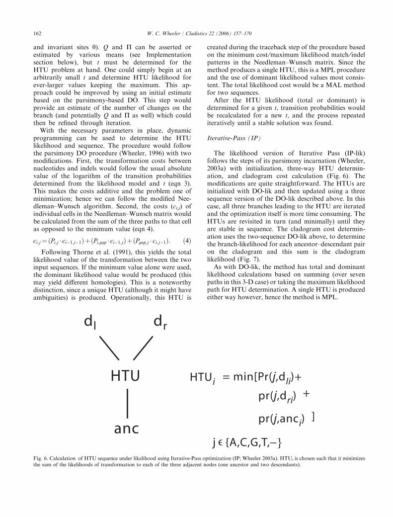
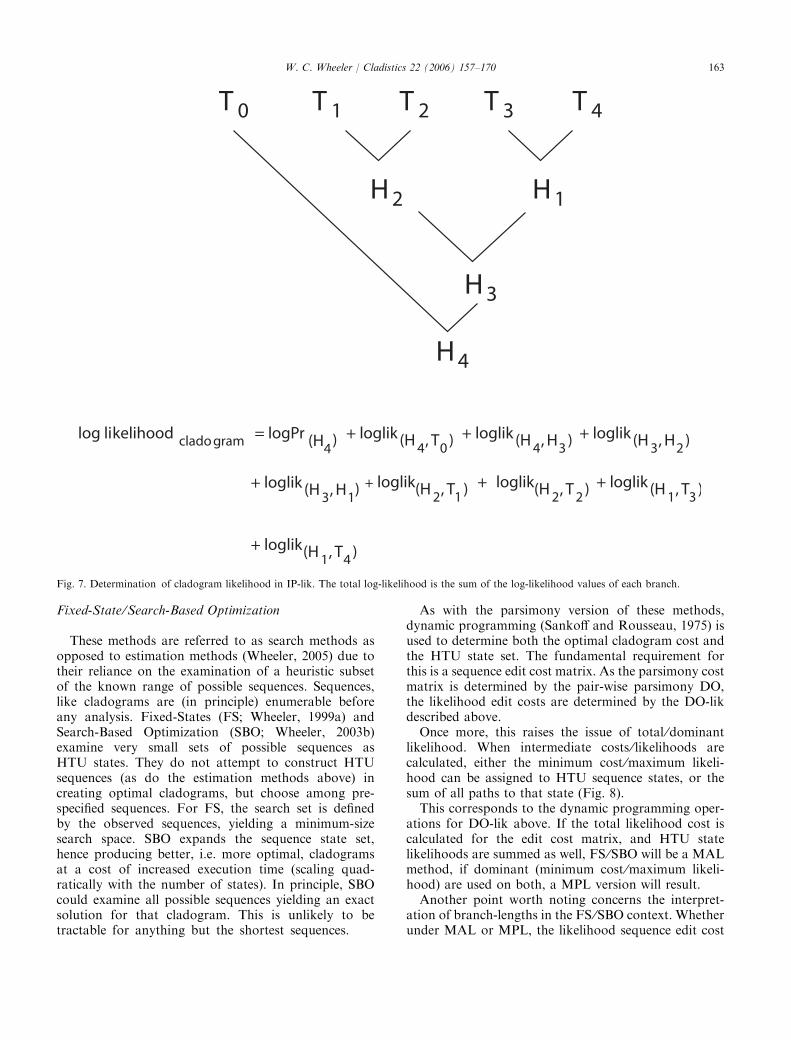
The likelihood version of Iterative Pass (IP-lik)follows the steps of its parsimony incarnation (Wheeler,2003a) with initialization, three-way HTU determin-ation, and cladogram cost calculation (Fig. 6). Themodifications are quite straightforward. The HTUs areinitialized with DO-lik and then updated using a threesequence version of the DO-lik described above. In thiscase, all three branches leading to the HTU are iteratedand the optimization itself is more time consuming. TheHTUs are revisited in turn (and minimally) until theyare stable in sequence. The cladogram cost determin-ation uses the two-sequence DO-lik above, to determinethe branch-likelihood for each ancestor–descendant pairon the cladogram and this sum is the cladogramlikelihood (Fig. 7).

As with DO-lik, the method has total and dominantlikelihood calculations based on summing (over sevenpaths in this 3-D case) or taking the maximum likelihoodpath for HTU determination. A single HTU is producedeither way however, hence the method is MPL.

Fig. 6. Calculation of HTU sequence under likelihood using Iterative-Pass optimization (IP; Wheeler 2003a). HTUi is chosen such that it minimizesthe sum of the likelihoods of transformation to each of the three adjacent nodes (one ancestor and two descendants).


Fixed-State ⁄Search-Based Optimization

These methods are referred to as search methods asopposed to estimation methods (Wheeler, 2005) due totheir reliance on the examination of a heuristic subsetof the known range of possible sequences. Sequences,like cladograms are (in principle) enumerable beforeany analysis. Fixed-States (FS; Wheeler, 1999a) andSearch-Based Optimization (SBO; Wheeler, 2003b)examine very small sets of possible sequences asHTU states. They do not attempt to construct HTUsequences (as do the estimation methods above) increating optimal cladograms, but choose among pre-specified sequences. For FS, the search set is definedby the observed sequences, yielding a minimum-sizesearch space. SBO expands the sequence state set,hence producing better, i.e. more optimal, cladogramsat a cost of increased execution time (scaling quad-ratically with the number of states). In principle, SBOcould examine all possible sequences yielding an exactsolution for that cladogram. This is unlikely to betractable for anything but the shortest sequences.

As with the parsimony version of these methods,dynamic programming (Sankoff and Rousseau, 1975) isused to determine both the optimal cladogram cost andthe HTU state set. The fundamental requirement forthis is a sequence edit cost matrix. As the parsimony costmatrix is determined by the pair-wise parsimony DO,the likelihood edit costs are determined by the DO-likdescribed above.

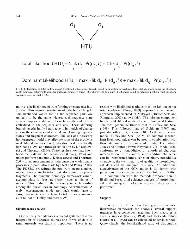
Once more, this raises the issue of total ⁄dominantlikelihood. When intermediate costs ⁄ likelihoods arecalculated, either the minimum cost ⁄maximum likeli-hood can be assigned to HTU sequence states, or thesum of all paths to that state (Fig. 8).

This corresponds to the dynamic programming oper-ations for DO-lik above. If the total likelihood cost iscalculated for the edit cost matrix, and HTU statelikelihoods are summed as well, FS ⁄SBO will be a MALmethod, if dominant (minimum cost ⁄maximum likeli-hood) are used on both, a MPL version will result.

Another point worth noting concerns the interpret-ation of branch-lengths in the FS ⁄SBO context. Whetherunder MAL or MPL, the likelihood sequence edit cost

Fig. 7. Determination of cladogram likelihood in IP-lik. The total log-likelihood is the sum of the log-likelihood values of each branch.


matrix is the likelihood of transforming one sequence intoanother. This requires an estimate of t, the branch length.The likelihood values for all the sequence pairs areunlikely to be the same. Hence, each sequence statechange implies a different branch length and this isembedded in the sequence edit cost. These differingbranch lengths imply heterogeneity in models of changeamong the sequences and amixedmodel among sequencestates and fragment characters. The lack of a necessaryhomogeneous model may alleviate some of the problemsin likelihood analyses of real data, discussed theoreticallyby Chang (1996) and through simulation by Kolaczkow-ski and Thornton (2004). These results show that likeli-hood methods will be inconsistent (Chang, 1996) andunder-perform parsimony (Kolaczkowski and Thornton,2004) in an environment of heterogeneous evolutionaryprocesses (a point also made by Steel and Penny, 2000).The FS-SBO procedures do not truly create a mixedmodel among nucleotides, but do among sequencefragments. The dynamic homology framework cannotaccommodate (at least at present) such a mixing ofmodels. This is due to the necessary interrelationshipamong the nucleotides in homology determination. Atruly heterogeneous model approach would have toassign parameters to each nucleotide in some mannerakin to that of Tuffley and Steel (1998).

Simultaneous analysis

One of the great advances of recent systematics is theintegration of disparate sources and forms of data tosimultaneously test cladistic hypotheses. There is no

reason why likelihood methods must be left out of thetotal evidence (Kluge, 1989) approach (the Bayesianapproach implemented in MrBayes (Huelsenbeck andRonquist, 2003) allows this). The missing componenthas been likelihood models for morphological features.The most general of these is that of Tuffley and Steel(1998). This followed that of Goldman (1990) andpreceded others (e.g., Lewis, 2001). As the most generalmodel, Tuffley and Steel (NCM; no common mechan-ism) likelihood values can be used in combination withthose determined from molecular data. The r-statesJukes and Cantor (1969); Neyman (1971) model used,conforms to a nonadditive, or unordered characterinterpretation. Furthermore, since additive characterscan be transformed into a series of binary nonadditivecharacters, the vast majority of qualitative morphologi-cal data can be analyzed this way. An additionalattractiveness of the NCM model is its identity withparsimony (the same can be said for Goldman, 1990).

In combination with the methods proposed here, alikelihood-based total evidence analysis of morphologi-cal and unaligned molecular sequence data can beperformed.

Support

It is worthy of mention that given a commoninterpretive framework for analysis, several supportmeasures have convergent meaning. Such measures asBremer support (Bremer, 1994) and Jackknife values(Farris et al., 1996) can be calculated under likelihood.Quite clearly, the log-likelihood ratio of cladograms

Fig. 8. Calculation of total and dominant likelihood values under Search-Based optimization procedures. The total likelihood sums the likelihoodcontributions of all possible sequence state assignments at each HTU, whereas the dominant likelihood is found by determining the highest likelihoodsequence state for each HTU.


with and without a clade is identical to the Bremersupport, which is based on log-likelihood cladogramcosts. Jackknife values may prove to be especiallyinteresting if the summary cladogram is determinedfrom weighted (likelihood weighted) cladogram costs.The clade support values can be quite similar to thoseproposed as posterior probabilities by Bayesian phylo-genetic software (Huelsenbeck and Ronquist, 2003).This is an area for future investigation.

Implementation

An implementation was created in the computerprogram POY (Wheeler et al., 1996–2003, 2005a) toexplore these models and procedures. Several generaltopics merit discussion here, and more option specificinformation can be found in the POY documentation(ftp.amnh.org ⁄pub ⁄molecular ⁄poy).

Estimation of model parameters

Estimates of model parameters are required for HTUlikelihood calculations. In the most complex of cases,the 10 values of the R matrix, five of P, as well as thegamma shape parameter a and invariant sites propor-tion h will need to be determined (and the number ofdiscrete classes for the gamma shape distribution spe-cified). In general, these parameters can be calculated bytwo distinct methods: (1) before any search begins viapair-wise comparisons, or (2) during the search on abranch-by-branch basis.

The most simple and straightforward manner ofestimating R and P parameters is to perform a seriesof pair-wise parsimony alignments, enumerate thenumber of transitions of each type (including indels),and count the relative numbers of each nucleotide stateand gap. Such an empirical process would not be anexplicit attempt at maximizing any likelihood, butprovides a useful estimate. This could be refined byiterating the values of the parameters until a summedlikelihood value was optimized, but this would beextremely time consuming (PAUP (Swofford, 2003)can use a cladogram to estimate many parameters).Such a refinement for a and h would be quite reasonableand is the default for POY.

A second, more specific, estimation occurs during thedetermination of each HTU. A preliminary parsimonyalignment of the two descendant sequences (in the caseof DO-lik) or three adjacent sequences (in the case of IP-lik) could be used to estimate transition and statefrequency parameters specific to a branch of a clado-gram. The strength of such an estimate is that itwould be tailored to that area of a cladogram. Adrawback would be the large multiplication of effectiveparameters.

Estimation of branch lengths

An initial t (expected number of changes) is calculatedfrom parsimony DO and iteration proceeds from there.The branch length is incremented and decremented by afactor (step interval) and likelihoods recalculated. ForIterative Pass Optimizations, each of the three branchesconnected to the HTU are iterated in turn and repea-tedly until all are stable.

Dominant and total likelihood

As mentioned above, dominant and total likelihoodcosts can be calculated for DO-lik and IP-lik as well asthe FS ⁄SBO procedures. For reasons of efficiency,dominant likelihoods are usually calculated; hence, themethods are MPL by default. The only real difference inthe calculation for DO ⁄IP is found in Needleman andWunsch’s (1970) cell costs; summed for total likelihoodand maximum value for dominant.

For FS-lik ⁄SBO-lik, the total likelihood option isexact (given the state set) summing the likelihoods of allthe paths to a given state (i.e., from all others).

Combination of data

The combination of data for total evidence analysisproceeds by adding the log likelihoods of the componentcharacters. Qualitative morphological likelihoods aredetermined under No CommonMechanism (Tuffley andSteel, 1998). Molecular likelihood values are determinedby the analytical procedure (DO-lik, IP-lik, FS-lik orSBO-lik).

Cladogram likelihood

Cladogram log-likelihood is determined by summingthe log-likelihoods of the HTUs for DO-lik, the branchlog-likelihoods for IP, and the final root-state log-likelihoods for FS ⁄SBO with the log probability of theroot node.

An example

To illustrate the behavior of these methods, thearthropod data set of Giribet et al. (2001) was used.This data set contains 54 taxa, 303 morphologicalcharacters and eight molecular loci (16S mt rRNA, 18SrRNA, 28S rRNA, mt cytochrome c oxidase subunit I,elongation factor-1a, RNA Polymerase II, histone H3and U2 snRNA). Not all taxa were complete for all loci.Other examples can be found in Okusu et al., (2003) andEdgecombe and Giribet (2004).

All searches were performed using POY ver. 3.0.11(Wheeler et al., 1996–2003) on the AMNH DEMETER


cluster computer (2.8 GHz PIV Xeon CPU Linux) using50 processors. Searches were based on a single additionsequence, followed by TBR branch swapping and treefusing (Goloboff, 1999) if thereweremultiple cladograms.Up to 25 equally costly cladograms were stored, ran-domly adding new cladograms if the buffer were full(option fitchtrees). A final round of TBR swappingwas performed examining cladograms within 1% of theminimum cost to control errors in the cladogram lengthheuristic calculations. The following command lineoptions were used for all runs: -norandomizeout-group -treefuse -checkslop 10 -maxtrees 25-fitchtrees. Additionally, indel cost were set to twoand nucleotide substitutions to one. These would beconstant for parsimony, but revised under likelihood asmodel parameters (including indels) were estimated.Morphological changes were accorded a weight of twoto equal the indel cost, and this weighting was carriedthrough the likelihood analysis. Likelihood runs addedthe options -likelihood -totallikelihood-gammaclasses 2 -invariantsitesadjust touse the sum of dynamic homology alternatives (asopposed to the dominant likelihood), G rate distributionwith two classes (default), and adjustment for invariantsites. Likelihood calculations were based on the S6GF5

model (default) where nucleotide and indel frequencieswere initially estimated via pair-wise comparison andheldconstant over the search. The nucleotide–indel substitu-tion model (S6GF5) is equivalent to GTR+GAPS wherethere is a single indel transition probability for allnucleotides. This matrix was estimated, eigenvaluescalculated, and transition probabilities derived uniquelyfor each branch of each cladogram examined. Morpho-logical likelihood values were calculated using the meth-ods of Tuffley and Steel (1998).

These are not the analytical parameters used byGiribet et al. (2001) in their analysis. The searches herewere much less exhaustive and only a single (anddifferent) parameter set used. This was largely due tothe time requirements of the likelihood analyses.

Analyses were performed on each of the nine datapartitions (morphology and eight molecular loci) sepa-

rately and in combination. Each data set was analyzedunder likelihood and parsimony optimality criteriausing the four heuristic methods (except for the mor-phological data) described above, resulting in a total of78 analyses.

Results

The cladograms produced by the data set-criterion-heuristic combination are shown in Fig. 10. These aresummarized in Tables 1 and 2. As an example ofcomparative execution times, the 5S data set of Rede-lings and Suchard (2005) required 8 s on a 2.4 GHz PIIIrunning Linux to complete a simple search with TBRbranch swapping using Direct Optimization and FixedStates, and 86 s for Iterative-Pass. Their 12 taxon EF-1adata set (as DNA not the amino acids originallyanalyzed) required 1072 s for Direct Optimization and7 s for Fixed States, both supporting their ‘‘eocyte’’result.

Morphological analysisParsimony analysis of the 303 morphological charac-

ters resulted in 12 cladograms of length 596, while

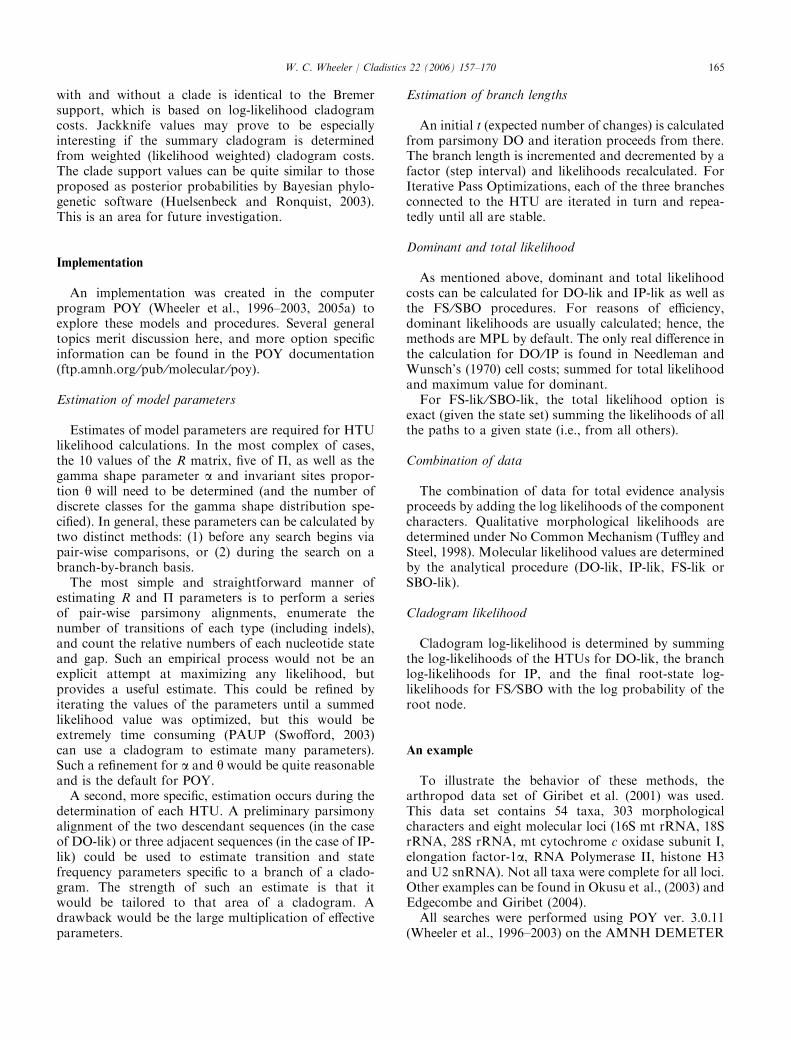
Table 1Optimality values for partition analyses under parsimony and likelihood (-log). Data of Giribet et al. (2001)

Optimality Method

Cladogram costs

Total Morph 16S 18S 28S COI EF1a H3 POL1 U2

Parsimony DO 35262 596 2865 13176 552 3311 5679 1189 4746 304IP 35006 596 2832 13027 546 3307 5689 1188 4751 305FS 42412 596 3477 14528 630 4541 7976 1507 6332 385SBO 37026 596 3204 14116 569 3383 5829 1209 4915 312

Likelihood DO 113090.23 766.90 6942.82 33611.75 2125.98 13033.37 23795.95 5427.81 17727.47 1477.40IP 113459.95 766.90 6892.47 33621.80 2147.69 13147.63 23619.13 5415.99 17835.97 1485.03FS 116570.82 766.90 7364.70 32242.45 1907.76 15789.13 28795.68 6037.71 21311.82 1497.24SBO 109441.22 766.90 6998.29 30431.90 1762.34 14456.72 25995.42 5730.46 20227.55 1358.63

Table 2Topological incongruence among data partitions under parsimony andlikelihood

Optimality Method

Topologicalcongruence

TILD RILD

Parsimony DO 0.495 0.691IP 0.422 0.699FS 0.450 0.751SBO 0.427 0.709

Likelihood DO 0.380 0.637IP 0.357 0.601FS 0.415 0.687SBO 0.409 0.703


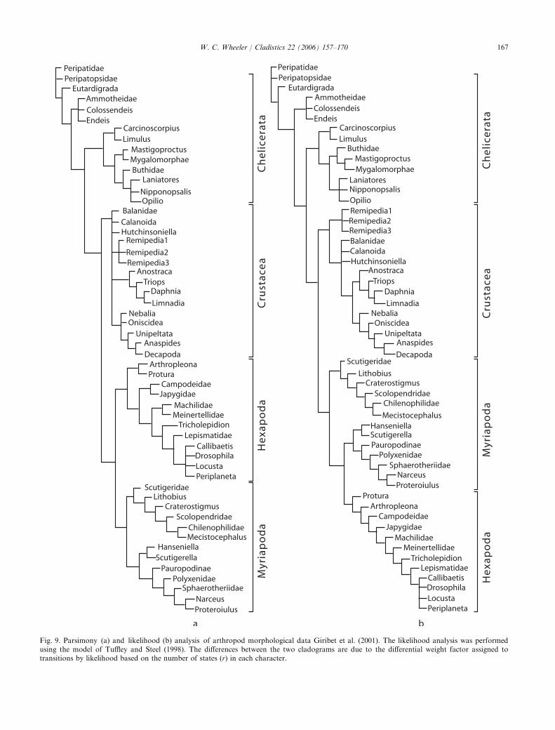
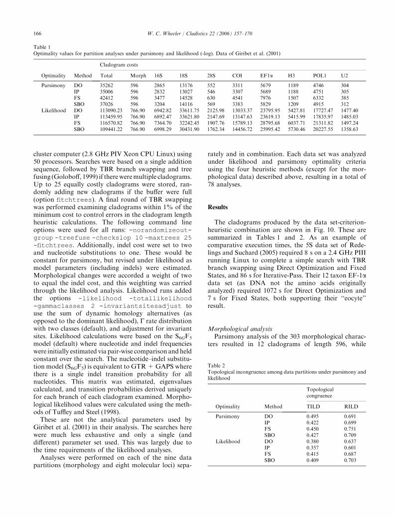
Fig. 9. Parsimony (a) and likelihood (b) analysis of arthropod morphological data Giribet et al. (2001). The likelihood analysis was performedusing the model of Tuffley and Steel (1998). The differences between the two cladograms are due to the differential weight factor assigned totransitions by likelihood based on the number of states (r) in each character.


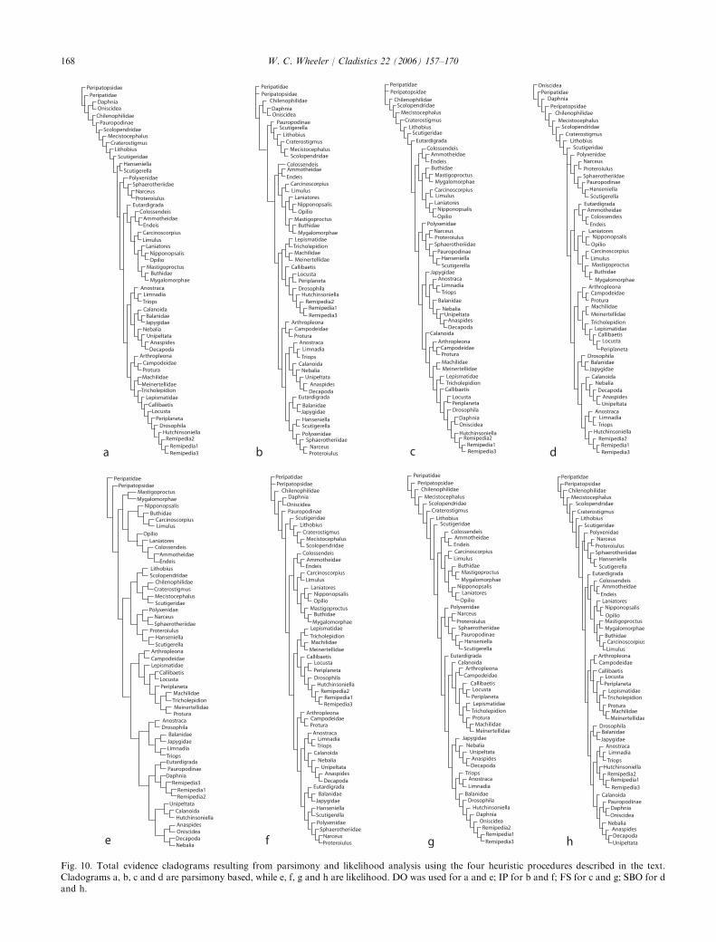
Fig. 10. Total evidence cladograms resulting from parsimony and likelihood analysis using the four heuristic procedures described in the text.Cladograms a, b, c and d are parsimony based, while e, f, g and h are likelihood. DO was used for a and e; IP for b and f; FS for c and g; SBO for dand h.


likelihood analysis resulted in 6 cladograms of cost 766.9(-log likelihood; Fig. 9). The consensus cladograms ofthese two analyses are largely similar, but with a fewdifferences (such asmyriapodmonophyly). It is often saidthat the Tuffley and Steel (1998) likelihood model showsthe identity of parsimony and likelihood however, this isnot strictly the case. In Tuffley and Steel (1998), theweight function of the contribution of an individualchange is inversely proportional to the number of states.Although a given character or a suite of characters withidentical numbers of states will yield identical results,data sets without such homogeneity will not, hence thedifferences between Figs 9a and b. The differences aresubtle but real.

Molecular lociThe individual cladograms for the molecular parti-

tions-optimality-heuristic procedure are contained in theaccessory materials. In general, the results of IP analyseswere superior (lower cost) to those of DO for parsimonybut not under likelihood. SBO outperformed FS forboth parsimony and likelihood.

Combined analysisStrict cladograms for these eight analyses are shown

in Fig. 10. The parsimony and likelihood results forSBO were identical. As expected, IP outperformed DOfor parsimony runs. FS were more costly than IP, DOand SBO. For the likelihood analysis, SBO was by farthe lowest cost (minimum -log lik) at 109 441.22 versus113 090.23 for DO (Table 1). This is consistent with theMAL version of likelihood employed here. SBOsummed the likelihoods (however marginal) of a largerset of potential HTU sequences than FS.

It is somewhat surprising that SBO outperformed allthe other heuristics,whichwas not the case for parsimony.While the parsimony scores for the heuristics can becompared (since the tree lengths all represent the sameweighted sum of events), it is not clear if the likelihoodscan be. Certainly FS and SBO can be compared, as theyare attempting to do the same thing (using the same formof likelihood and HTU determination). The estimationheuristics (DO and IP) are approaching the likelihoodproblem in a very different way.

Comparison

The numerical values (character congruence) pro-duced by likelihood and parsimony analyses are largelyincomparable. In order to assess their behavior, acomparison can be made, however, through an analysisof topological consistency among data partitions. Suchan analysis was performed here using the topologicalincongruence metrics of Wheeler (1999b; Table 1).

Overall, parsimony outperformed likelihood, witheach heuristic procedure having higher topologicalcongruence values (TILD or RILD) for the parsimonyversion. These differences are not great (about 9% forthe TILD values and 7.5% for RILD) and it is hard tosay whether such distinctions are significant in astatistical sense. Furthermore, given the abbreviatednature of the searches and parameter space explored,this example is more of a demonstration than a generalanalysis of a congruence-based comparison technique.

The heuristics that yielded the highest congruence arethe Search-Based FS and SBO. This holds for bothparsimony and likelihood. While SBO also yielded thebest likelihood score, this was not true of parsimony.The Search-Based techniques have the virtue of conver-ging on an exact solution as the potential state setenlarges, for both optimality criteria. This convergencebehavior may be keeping the partitions more consistentwith each other as they add additional HTU options.

Discussion

The simple models presented here show that likelihoodmethods can be applied to scenarios of dynamic homol-ogy and combined analysis for real-sized data sets. Thisenlarges the world of problems amenable to likelihoodanalysis and allows us to bring to bear the greatestdiversity of evidence to systematic problems within thisprobabilistic framework. More parameterized models(including affine gaps, lineage heterogeneity, etc.) mightwell improve the quality of the likelihood results, but theapproximate techniques employed here are certainlyusable now and provide a productive heuristic for moreelaborate and time-consuming procedures.

Acknowledgments

I would like to thank Illya Bomash, Louise Crowley,Torsten Erikson, Gonzalo Giribet, Pablo Goloboff,Taran Grant, Cyrille D’Haese, Daniel Janies, JeromeMurienne, Vamsikrishna Kalapala, Kurt Pickett,Usman Roshan, Wm. Leo Smith, Steven Thurston,Andres Varon and two anonymous reviewers for manyhelpful critisms of the manuscript and the support of theFundamental Space Biology Program of NASA.

References

Barry, D., Hartigan, J., 1987. Statistical analysis of hominid molecularevolution. Stat. Sci. 2, 191–210.

Bishop, M.J., Thompson, E.A., 1986. Maximum likelihood alignmentof DNA sequences. J. Mol. Biol. 190, 159–165.

Bremer, K., 1994. Branch support and tree stability. Cladistics, 10,295–304.


Chang, J.T., 1996. Inconsistency of evolutionary tree topologyreconstruction methods when substitution rates vary across char-acters. Math. Bio. 134, 189–215.

Durbin, R., Eddy, S.R., Krogh, A., Mitchison, G., 1998. BiologicalSequence Analysis: Probabilistic Models of Proteins and NucleicAcids. Cambridge University Press, Cambridge, UK.

Edgecombe, G.D., Giribet, G., 2004. Molecular phylogeny of austra-lasian anopsobiine centipedes (Chilopoda: Lithobiomorpha). Inv.Syst. 18, 235–249.

Farris, J.S., 1973. A probability model for inferring evolutionary trees.Syst. Zool. 22, 250–256.

Farris, J.S., Albert, V.A., Kallersjo, M., Lipscomb, D., Kluge, A.G.,1996. Parsimony jackknifing outperforms neighbor-joining.Cladistics, 12, 99–124.

Fleissner, R., Metzler, D., von Haeseler, R., 2005. Simultaneousstatistical mulitple alignment and phylogeny reconstruction. Syst.Biol. 54, 548–561.

Giribet, G., Edgecombe, G.D., Wheeler, W.C., 2001. Arthropodphylogeny based on eight molecular loci and morphology. Nature,413, 157–161.

Goldman, N., 1990. Maximum likelihood inference of phylogenetictrees, with special reference to a poisson process model of dnasubstitution and to parsimony analysis. Syst. Zool. 39, 345–361.

Goloboff, P., 1999. Analyzing large data sets in reasonable times:solutions for composite optima. Cladistics, 15, 415–428.

Goloboff, P.A., 2003. Parsimony, likelihood, and simplicity. Cladistics,19, 91–103.

Hein, J.C., Jensen, J.L., Pedersen, C.N.S., 2003. Recursions forstatistical multiple alignment. Proc. Natl Acad. Sci. USA, 100,14960–14965.

Hein, J., Wiuf, C., Knudsen, B., Moller, M.B., Wibling, G., 2000.Statistical alignment: computational properties, homology testing,and goodness-of-fit. J. Mol. Biol. 302, 265–279.

Huelsenbeck, J.P., Ronquist, F., 2003. MrBayes: Bayesian inference ofphylogeny, 3.0 edition. Program and documentation available athttp://morphbank.uuse/mrbayes/.

Jukes, T.H., Cantor, C.R., 1969. Evolution of protein molecules. In:Munro, N.H. (Ed.), Mammalian Protein Metabolism. AcademicPress, New York, pp. 21–132.

Kluge, A.G., 1989. A concern for evidence and a phylogenetichypothesis of relationships among Epicrates (Boidae, Serpentes).Syst. Zool. 38, 7–25.

Kolaczkowski, B., Thornton, J.W., 2004. Performance of maximumparsimony and likelihood phylogenetics when evolution is hetero-geneous. Nature, 431, 980–984.

Lewis, P.O., 2001. A likelihoods approach to estimating phylogeny fromdiscrete morphological character data. Syst. Biol. 50, 913–925.

McGuire, G., Denham, M.C., Balding, D.J., 2001. Balding: Models ofsequence evolution for dna sequences containing gaps. Mol. Biol.Evol. 18, 481–490.

Needleman, S.B., Wunsch, C.D., 1970. A general method applicable tothe search for similarities in the amino acid sequences of twoproteins. J. Mol. Biol. 48, 443–453.

Neyman, J., 1971. Molecular studies in evolution: a source of novelstatistical problems. In: Gupta, S.S., Yackel, J. (Eds.), StatisticalDecision Theory and Related Topics. Academic Press, New York,pp. 1–27.

Okusu, A., Schwabe, E., Eernisse, D.J., Giribet, G., 2003. Towardsa phylogeny of chitons (mollusca, polyplacophora) based oncombined analysis of five molecular loci. Org. Divers. Evol. 3,281–302.

Redelings, B.D., Suchard, M.A., 2005. Joint Bayesian estimation ofalignment and phylogeny. Syst. Biol. 54, 401–418.

Sankoff, D.M., 1975. Minimal mutation trees of sequences. SIAM. J.Appl. Math, 28, 35–42.

Sankoff, D.M., Rousseau, P., 1975. Locating the vertices of a Steinertree in arbitrary space. Math. Program. 9, 240–246.

Slowinski, J.B., 1998. The number of multiple alignments. Mol.Phylogen. Evol. 10, 264–266.

Steel, M., 2002. Some statistical aspects of the maximum parsimonymethod. In: Desalle, R., Giribet, G., Wheeler, W.C. (Eds.),Techniques in Molecular Systematics and Evolution. Birkhauser-Verlag, Basel, Switzerland, pp. 124–140.

Steel, M., Hein, J., 2001. Applying the Thorne-Kishino-Felsensteinmodel to sequence evolution on a star-shaped tree. Appl. Math.Let. 14, 679–684.

Steel, M., Penny, D., 2000. Parsimony, likelihood, and the role ofmodels in molecular phylogenetics. Mol. Biol. Evol. 17, 839–850.

Swofford, D.L., 2003. PAUP*: Phylogenetic analysis using parsimony(*and other methods), Version 4.0b.10. Sinauer Associates, Sun-derland, MA.

Tavare, S., 1986. Some probabilistic and statistical problems on theanalysis of DNA sequences. Lec. Math. Life Sci. 17, 57–86.

Thorne, J.L., Kishino, H., Felsenstein, J., 1991. An evolutionarymodel for maximum likelihood alignment of dna sequences. J. Mol.Evol. 33, 114–124.

Thorne, J.L., Kishino, H., Felsenstein, J., 1992. Inching toward reality:an improved likelihood model of sequence evolution. J. Mol. Evol.34, 3–16.

Tuffley, C., Steel, M., 1998. Links between maximum likelihood andmaximum parsimony under a simple model of site substitution.Bull. Math. Biol. 59, 581–607.

Wang, L., Jiang, T., 1994. On the complexity of multiple sequencealignment. J. Computational Biol. 1, 337–348.

Wheeler, W.C., 1996. Optimization alignment: The end of multiplesequence alignment in phylogenetics? Cladistics, 12, 1–9.

Wheeler, W.C., 1999a. Fixed character states and the optimization ofmolecular sequence data. Cladistics, 15, 379–385.

Wheeler, W.C., 1999b. Measuring topological congruence by extend-ing character techniques. Cladistics, 15, 131–135.

Wheeler, W.C., 2001. Homology and the optimization of DNAsequence data. Cladistics, 17, S3–S11.

Wheeler, W.C., 2003a. Iterative pass optimization. Cladistics, 19, 254–260.

Wheeler, W.C., 2003b. Search-based character optimization. Cladis-tics, 19, 348–355.

Wheeler, W.C., 2005. Alignment, dynamic homology, and optimiza-tion. In: Albert, V. (Ed.), Parsimony, Phylogeny, and Genomics.Oxford University Press, pp. 73–80.

Wheeler, W.C., Aagesen, L., Arango, C.P., Faivoich, J., Grant, T.,D’Haese, C., Janies, D., Smith, W.L., Varon, A., Giribet, G.,2005a. Dynamic Homology and Systematics: A Unified Approach.American Museum of Natural History.

Wheeler, W.C., Aagesen, L., Arango, C.P., Faivovich, J., Grant, T.,D’Haese, C.A., Janies, D., Smith, W.L., Varon, A., Giribet, G.,2005b. Dynamic Homology and Phylogenetic Systematics: AUnified Approach Using POY. American Museum of NaturalHistory.

Wheeler, W.C., Gladstein, D.S., Laet, J.D., 1996–2003. POY, 3.0.11edition, 1996–2003. ftp.amnh.org ⁄pub ⁄molecular ⁄poy (currentversion 3.0.11). Documentation by D. Janies and W. Wheeler.Commandline Documentation by J. De Laet and. W. C. Wheeler.

Yang, Z., 1994. Estimating the pattern of nucleotide substitution.J. Mol. Evol. 39, 105–111.


Wheeler, W.C. 2006.

Documents

Transcript of Wheeler, W.C. 2006.