1

WHAT IS (PROPENSITY SCORE) MATCHING?

Barbara Sianesi

PEPA node of NCRM, Institute for Fiscal Studies

5th ESRC Research Methods Festival

Oxford, July 2012

2

(PS)MATCHING IS EXTREMELY POPULAR…

→ 270,000 entries by googling: propensity score matching

→ 13,000 downloads of –psmatch2–

501st of 1,100,000 items in the RePEc/IDEA database

→ >1,500 support emails

� Europe, US, Canada, Central + South America, former SU, Australia, Asia, Africa and the Middle East

� epidemiology, sociology, economics, statistics, criminology, agricultural economics, health economics, transport economics, public health, nutrition, paediatrics, biostatistics, finance, urban planning, geography and geosciences

3

WHAT IS (PS)MATCHING?

(PS)Matching is a method/device to make two groups look the same.

4

1. The counterfactual concept of causality

2. What is matching?

3. How do we use it?

4. Should we use it?

5

THE COUNTERFACTUAL CONCEPT OF CAUSALITY

The Evaluation Problem

to evaluate average causal effects of a ‘treatment’ on an outcome.

The Potential Outcome model

Y1 Outcome under treatment

Y0 Outcome without treatment

YYYY1111 ––––YYYY0000 Treatment effect

D ∈ {0, 1} Treatment indicator

� � �� � � 0� �� � � 1 � Observed outcome

X Set of observed characteristics

6

The parameters of interest

� ATT ≡ E(Y1 – Y0 | D�1) � E(Y | D�1) – EEEE((((YYYY0000 | | | | DDDD�1)�1)�1)�1) � ATNT ≡ E(Y1 – Y0 | D�0) � EEEE((((YYYY1111 | | | | DDDD�0)�0)�0)�0) – E(Y | D�0) � ATE ≡ E(Y1 – Y0 ) � ATT⋅P(D�1) +ATNT⋅P(D�0) The Fundamental Problem of Causal Inference

Need to invoke (untestable) assumptions to identify average unobserved counterfactuals.

MATCHING METHODS – INTUITION (FOR ATT) Ex post mimic a RCT by constructing a suitable comparison group by carefully matching treated and non-treated

→ selected comparison group is as similar as possible to the treatment group…in terms of their observable characteristics

7

MATCHING METHODS – ASSUMPTIONS

1. Identifying assumption: Selection on Observables (conditional independence CIA, exogeneity, ignorability, unconfoundedness) All the relevant differences between treated and non-treated are captured in X:

ATT: E(Y0 | X, D�1) � E(Y0 | X, D�0) ATNT: E(Y1 | X, D�1) � E(Y1 | X, D�0) ATE: both

2. To give it empirical content: Common Support

We observe participants and non-participants with the same characteristics:

ATT: P(D�1 | X) < 1 ATNT: 0 < P(D�1 | X) ATE: 0 < P(D�1 | X) <1

⇒ can use the (observed) mean outcome of the non-treated to estimate the mean (counterfactual) outcome the treated would have had they not been treated.

8

OPERATIONALISING MATCHING METHODS

Curse of dimensionality

- impose linearity in the parameters (regression analysis)

- choose a distance metric

� Mahalanobis metric

d(i,j) = (Xi – Xj)' V-1

(Xi – Xj)

� Propensity Score p(x) ≡ P(D=1| X=x) Conditional treatment probability (given confounders X)

The propensity score is a balancing score, i.e.

X ⊥ D | p(X)

If CIA holds given X → CIA holds given p(X)

9

Overview of Matching Estimators

1. pair to each treated i some group of ‘comparable’ non-treated individuals

2. associate to the outcome yi of treated i, a matched outcome ˆiy given by the

(weighted) outcomes of his ‘neighbours’ in the comparison group:

0( )

ˆ

i

i ij j

j C p

y w y∈

= ∑

• C0(pi) = set of neighbours of treated i in the D=0 group

• wij = weight on non-treated j in forming a comparison with treated i, where 0

( )

1

i

ij

j C p

w∈

=∑

General form of the matching estimator for ATT (within S10):

{ }{10

10

^

{ 1 }#( 1 )

1ˆ

i

i i

i D SD S

ATT y y∈ = ∩

= ∩= −∑

= E(Y | treated on S10) – E(Y | matched/reweighted non-treated)

10

TRADITIONAL MATCHING ESTIMATORS

One-to-one matching

− with or without replacement

− nearest neighbour or within caliper SIMPLE SMOOTHED MATCHING ESTIMATORS

• K-nearest neighbours

− with or without replacement

− nearest neighbour or within caliper

• Radius matching WEIGHTED SMOOTHED MATCHING ESTIMATORS

• Kernel-based matching

• Local linear regression-based matching � bandwidth choice � kernel choice

11

Checking matching quality

Check (and possibly improve on) balancing of observables

- for each variable

- overall measures

Inference

- naïve variance

- bootstrapping

- Abadie-Imbens heteroskedasticity-robust standard errors when matching on X

- Abadie-Imbens analytical asy std errors taking into account estimation of e(X) for PS nearest neighbour(s) matching with replacement

ˆ( )D X p X⊥ |

12

MATCHING VS OLS

- same identifying assumption

If unobserved confounders, just as biased as OLS – internal validity

- avoids any additional assumption

(1) COMMON SUPPORT

Matching performed only over Sup10, hence compares only comparable people

Might recover a different causal impact: ATT(Sup10) ≠ ATT (Sup1) – external validity

(2) NON-PARAMETRIC

Avoids potential misspecification of E(Y0 | X)

Allows for arbitrary X-heterogeneity in impacts E(Y1 – Y0 | X)

⇒ Matching focuses on comparability in terms of observables, i.e. on constructing a suitable comparison group by carefully matching treated and non-treated on X / reweighting the non-treated to realign their X

But: if OLS is correctly specified, OLS is more efficient.

13

BUT we don’t need matching to make OLS less parametric…

FULLY INTERACTED OLS -FILM-

0 1 2 1 1 2 2 12 1 2( , ) ( ) ( ) ( )Y m X X D X D X D X X D eδ δ δ δ= + + + + +

1 1 2 2 12 1 2 11 1( )ATT DD D

X X X Xβ δ δ δ δ | =| = | == + + +

1 1 2 2 12 1 2 00 0( )ATNT DD D

X X X Xβ δ δ δ δ | =| = | == + + +

1 1 2 2 12 1 2( )ATE X X X Xβ δ δ δ δ= + + +

Can F-test for presence of heterogeneous effects.

14

STILL, matching (≠≠≠≠ OLS) highlights comparability of groups

Check matching quality

• Propensity score – more ‘structural’ model – more flexible specification – probit/logit – probability/index/odds ratio

• Matching – metric: X, ˆ ( )p X or {X, ˆ ( )p X }

– type of matching – smoothing parameters – common support

• Assessment of matching quality

CAN we get the two groups balanced (in terms of X)? [Think back to RCT…]

15

STRENGTHS AND WEAKNESSES

☺ Advantages ☺

• controls for selection on observables and on observably heterogeneous impacts

• non-(or semi-) parametric: no specific form for outcome equation, decision process or either unobservable term

• Sup10: compare only comparable people and help determining which results reliable

• flexible and easy

� Disadvantages �

• selection on observables: matching as good as its X’s

• restricting to Sup10 may change parameter being estimated → unable to identify ATT

• data hungry

16

EXAMPLE: IMPACT OF NSW

Very famous data in the evaluation literature, combining treatment and controls from a randomised evaluation of the NSW Demonstration with non-experimental individuals drawn from various sources. NSW male treated (297) with male comparisons drawn from the PSID (2,490) Y = real earnings in 1978 X = age, ethnicity (black and hisp), education (years and <12 years), real pre-

programme earnings in 1975

17

COMPARABILITY OF GROUPS

NSW trainees vs NSW control group

True ATT (experimental estimator) = 886*

18

NSW trainees vs PSID comparison group

→ expect naïve comparison to be downward biased

Naïve estimator = -15,578***

19

Distribution of ˆ( )p X

NSW treated PSID comparisons

20

NSW trainees vs matched PSID comparison group – nearest neighbour (w/ replac)

21

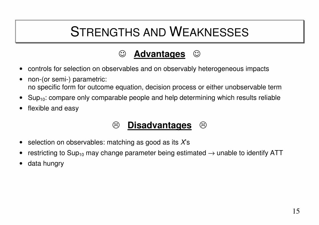
NSW trainees vs matched PSID comparison group – Mahal on X and p(X)

22

Achieved balancing

Randomisation Nearest Neighbour, with replacement Mahalanobis

Kernel (epan, h=0.01) Radius (r=0.01) Augmented Mahalanobis

-20 -15 -10 -5 0 5 10 15 20Standardized % bias across covariates

nodegree

hispanic

black

re75

age

married

educ

-20 -15 -10 -5 0 5 10 15 20Standardized % bias across covariates

age

re75

black

hispanic

nodegree

educ

married

-20 -15 -10 -5 0 5 10 15 20Standardized % bias across covariates

re75

educ

age

black

hispanic

married

nodegree

-20 -15 -10 -5 0 5 10 15 20Standardized % bias across covariates

re75

black

age

nodegree

hispanic

married

educ

-20 -15 -10 -5 0 5 10 15 20Standardized % bias across covariates

re75

black

nodegree

age

hispanic

married

educ

-20 -15 -10 -5 0 5 10 15 20Standardized % bias across covariates

educ

age

re75

married

black

hispanic

nodegree

23

How many PSID members are we really using?

Nearest neighbour (w/ replac) Kernel (Epan, h=0.01)

24

Impact estimates

True ATT (experimental estimator) 886* Naïve estimator -15,578*** OLS -1,458* FILM -1,361* Nearest neighbour (w/ replacement) 551 Kernel (Epan, h=0.01) -737 Augmented Mahalanobis -830

25

ATNT Average effect of NSW programme had the PSID participated in it Kernel PS matching (epan, h=0.06)

Fully interacted regression model

26

Nearest neighbour Kernel (Epan, h=0.06)

27

ATNT: –12,580*** (matching) º –12,468*** (film)

Good the PSID did not go into the programme! Or is it…? And now that we are thinking about it… Do we really want to know the impact the NSW would have had on the full PSID has they participated?!?

28

WRAPPING UP…

SELECTION ON UNOBSERVABLES

• Set of conditioning X matters

⇒ better data help a lot!

SELECTION ON OBSERVABLES

• Avoid use of functional forms in constructing counterfactual

⇒ (matching ≈ fully interacted OLS) � simple OLS no mis-specification bias

• Compare comparable people

⇒ matching � fully interacted OLS highlight – actual comparability of groups,

– hence reliability (& relevance) of estimates

29

SELECTED REFERENCES

A comprehensive review

Imbens, G. (2004), ‘Semiparametric estimation of average treatment effects under exogeneity: a review’, Review of Economics and Statistics, 86, 4-29.

The propensity score

Rosenbaum, P.R. and Rubin, D.B. (1983), “The Central Role of the Propensity Score in Observational Studies for Causal Effects”, Biometrika, 70, 41-55.

Rosenbaum, P.R. and Rubin, D.B. (1984), “Reducing Bias in Observational Studies Using Sub-Classification on the Propensity Score”, Journal of the American Statistical Association, 79, 516-524.

Rosenbaum, P.R. and Rubin, D.B. (1985), “Constructing a Control Group Using Multivariate Matched Sampling Methods that Incorporate the Propensity Score”, The American Statistician, 39, 1, 33-38.

Dehejia, R.H. and Wahba, S. (1999), “Causal Effects in Non-Experimental Studies: Re-Evaluating the Evaluation of Training Programmes”, Journal of American Statistical Association, 94, 1053-1062.

Heckman, J.J., Ichimura, H. and Todd, P.E. (1997), “Matching As An Econometric Evaluation Estimator: Evidence from Evaluating a Job Training Programme”, Review of Economic Studies, 64, 605-654.

Heckman, J.J., Ichimura, H. and Todd, P.E. (1998), “Matching as an Econometric Evaluation Estimator”, Review of Economic Studies, 65, 261-294.

30

Mahalanobis-metric matching

Rubin, D.B. (1979), “Using Multivariate Matched Sampling and Regression Adjustment to Control Bias in Observational Studies”, Journal of the American Statistical Association, 74, 318-328.

Rubin, D.B. (1980), “Bias Reduction Using Mahalanobis-Metric Matching”, Biometrics, 36, 293-298.

Multiple treatments

Imbens, G.W. (2000), “The Role of Propensity Score in Estimating Dose-Response Functions”, Biometrika, 87, 706-710.

Lechner, M. (2001), Identification and Estimation of Causal Effects of Multiple Treatments under the Conditional Independence Assumption, in: Lechner, M., Pfeiffer, F. (eds), Econometric Evaluation of Labour Market Policies, Heidelberg: Physica/Springer, 43-58.

Inference/Efficiency issues

Abadie, A. and Imbens, G. (2011), “Matching on the Estimated Propensity Score”, mimeo.

Abadie, A. and Imbens, G. (2006), “Large Sample Properties of Matching Estimators for Average Treatment Effects”, Econometrica, 74, 235-267.

Hahn, J. (1998), “On the Role of the Propensity Score in Efficient Semiparametric Estimation of Average Treatment Effects,” Econometrica, 66, 315-331.

Hirano, K., G. Imbens, and G. Ridder (2003), “Efficient Estimation of Average Treatment Effects Using the Estimated Propensity Score,” Econometrica, 71, 1161-1189.