What Have They Been Thinking? Homebuyer Behavior in … · 265 karl e. case Wellesley College...

265

karl e. caseWellesley College

robert j. shillerYale University

anne k. thompsonMcGraw-Hill Construction

What Have They Been Thinking? Homebuyer Behavior in Hot

and Cold Markets

ABSTRACT Questionnaire surveys undertaken in 1988 and annually from 2003 through 2012 of recent homebuyers in each of four U.S. metropoli-tan areas shed light on their expectations and reasons for buying during the recent housing boom and subsequent collapse. They also provide insight into the reasons for the housing crisis that initiated the current financial malaise. We find that homebuyers were generally well informed, and that their short-run expectations if anything underreacted to the year-to-year change in actual home prices. More of the root causes of the housing bubble can be seen in their long-term (10-year) home price expectations, which reached abnormally high levels relative to mortgage rates at the peak of the boom and have declined sharply since. The downward turning point, around 2005, of the long boom that preceded the crisis was associated with changing public understanding of speculative bubbles.

between the end of World War II and the early 2000s, the U.S. hous-ing market contributed much to the strength of the macroeconomy. It

was a major source of jobs, produced consistently rising home equity, and served as perhaps the most significant channel from monetary policy to the real economy. But starting with a drop in the S&P/Case-Shiller Home Price Index for Boston in September 2005, home prices began to fall in city after city. By the time the slump was over, prices were down almost 32 per-cent on a national basis, with many cities down by more than 50 percent,

266 Brookings Papers on Economic Activity, Fall 2012

wiping nearly $7 trillion in equity off household balance sheets. The pro-duction of new homes and apartments, as measured by housing starts, peaked in January 2006 at 2.27 million on an annual basis. Starts then fell 79 percent, to fewer than 500,000, in just 2 years. From October 2008 until September 2012—a stretch of 48 months—starts remained below a season-ally adjusted annualized rate of 800,000 units, a 50-year-low.

As prices fell, the mortgage industry collapsed and the entire financial system was shaken to its core. Even mortgages and mortgage-backed secu-rities that had been well underwritten went into default. Very high rates of default and foreclosure sent Fannie Mae and Freddie Mac, the two main government-sponsored enterprises in the housing finance industry, into receivership and led to the failure of the investment banks Lehman Brothers and Bear Stearns in 2008. The economy went into a severe reces-sion in the fourth quarter of 2007. A similar pattern infected housing markets around the world, including parts of the euro zone and China.

What do we know and what do we need to know about the forces that led to this huge failure of such a large market? The literature on the housing boom and bust of the 2000s is extensive and has identified several potential cul-prits: a growing complacency of lenders in the face of declining loan qual-ity (Mian and Sufi 2009, Demyanyk and van Hemert 2011); money illusion on the part of homebuyers that led to flawed comparisons of home purchase prices with rents (Brunnermeier and Julliard 2008, along lines exposited by Modigliani and Cohn 1979 for the stock market); an agency problem afflict-ing the credit rating agencies (Mathis, McAndrews, and Rochet 2009); and government failure to regulate an emerging shadow banking system (Gorton 2010). Most if not all of these certainly contributed, even if their relative importance remains unknown. But one thing that is known is that what happens in the housing market depends on the behavior and attitudes of mil-lions of individual participants, and foremost among them are homebuyers.

We believe that one aspect of this episode has not received the attention that it deserves: the role of homebuyers’ expectations. What were people thinking when they bought a home? At the time of purchase, a buyer of a capital asset is buying a flow of services and benefits that will all come in the future, and the future is always uncertain. Buying a home means mak-ing a series of very difficult decisions that will in all likelihood affect the buyers’ lives forever. Anyone who has ever signed an offer sheet, read a building inspector’s report, or written a down payment check, and won-dered what would happen if she lost her job or fell seriously ill, knows that these decisions are emotional, personal, and difficult. The title of this paper focuses on this process of thinking about the future that homebuyers go

karl e. case, robert j. shiller, and anne k. thompson 267

through—calculating subjective costs, weighing risks and one’s own toler-ance for risk, formulating and trading off among preferences—all difficult topics for economists. Understanding the housing market is really about understanding what goes on in the minds of buyers, and we chose to go directly to the source.

This paper reports and analyzes results of a series of surveys that we have conducted since 1988 of homebuyers in four metropolitan areas nationwide. We begin with a description of the survey, of the questionnaire itself, and of the sample sizes. The bulk of the paper then asks and attempts to answer, using the survey data, a number of questions that, we think, will add to our understanding of how the housing market works:

—Do homebuyers know what the trends in housing prices are in their metro area at the time of the survey?

—What do homebuyers expect to happen to the value of their home in the next year and over 10 years?

—Are homebuyers’ expectations rational, and how are they formed?—What brought the early-2000s housing bubble to an end?—What caused the rebound in the market in 2009–10, and why did it

fizzle?The choice of questions is constrained by the nature of the data, and the

methodologies we use to answer them are simple and somewhat ad hoc, given that we lack a theoretical framework for our analysis. The roughly 5,000 respondents had one thing in common: they had purchased a home recently. Rather than look only at their actual behavior, we chose to ask about their perceptions, interpretations, and opinions. We singled out recent homebuyers in order to focus on the opinions of people who were actively involved in the process that determines home prices. We wanted to see how these opinions change through time. We cannot, however, assume that their responses describe the opinions of the great mass of people who were not actively participating in the housing market during this period.

I. Our Survey of Homebuyers

More than two decades ago, to gain a better understanding of the role of psychology and expectations in the housing market, we decided to survey a sample of homebuyers and ask them specifically about their reasons for buying. That survey, mailed in the late spring of 1988, consisted of a ques-tionnaire of approximately 10 pages, which we sent to a random sample of 500 homebuyers in each of four locations within metropolitan areas around the country: Alameda County, California (Oakland and much of the East


Bay, in the San Francisco-Oakland-Fremont, CA Metropolitan Statistical Area); Milwaukee County, Wisconsin (the core of the Milwaukee-Waukesha- West Allis, WI Metropolitan Statistical Area); Middlesex County, Mas-sachusetts (Cambridge and the areas north and west, in the Boston-Cambridge-Quincy, MA–NH Metropolitan Statistical Area), and Orange County, California (which includes Anaheim and Irvine in the southern part of the Los Angeles-Long Beach-Santa Ana, CA Metropolitan Statistical Area). These four were chosen to represent what were viewed at the time as two “hot” markets (Los Angeles and San Francisco), a “cold” (postboom) market (Boston), and a relatively stable market (Milwaukee).

The questionnaires were identical across the four survey locations. Par-ticipation was limited to people who had actually closed on a home that spring. In a typical year, only about 5 percent of the nationwide housing stock changes hands. Thus, our respondents do not necessarily represent the universe of homeowners, home seekers, or home sellers. Yet these are the people on whom we based our implicit valuation of the entire stock.

The response rate to that first survey was extraordinary: of 2,030 surveys mailed, 886, or 43.6 percent, were ultimately completed and tabulated. Case and Shiller (1988) presented the results of that survey and concluded, “While the evidence is circumstantial, and we can only offer conjectures, we see a market largely driven by expectations. People seem to form their expectations from past price movements rather than having any knowledge of fundamentals. This means that housing price booms will persist as home buyers become destabilizing speculators.” In addition, we found signifi-cant evidence that housing prices were inflexible downward, at least in the absence of severe and prolonged economic decline.

In 2003 we decided to replicate the survey in the same four counties, to see whether changes in market conditions and other recent history had changed people’s views. We have repeated the survey in the spring of each year since then. Except for the addition of some new questions at the end, the questionnaire has remained exactly the same in all surveys. We now have completed the process a total of 11 times, and this paper presents a first look at the aggregate results.

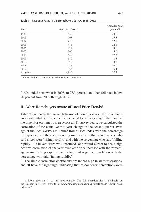
The response rate in the 2003 survey was 35.3 percent of 2,000 origi-nally mailed (table 1 shows the response rates for the whole series). The high response rate was in part the result of sending the questionnaire with a letter hand signed by both Case and Shiller, sending a postcard follow-up to nonrespondents, and finally sending a second mailing. When response rates dropped off after 2005, we included a letter signed by a colleague in each state. The response rate remained low in 2007, at 15 percent overall.


It rebounded somewhat in 2008, to 27.3 percent, and then fell back below 20 percent from 2009 through 2012.

II. Were Homebuyers Aware of Local Price Trends?

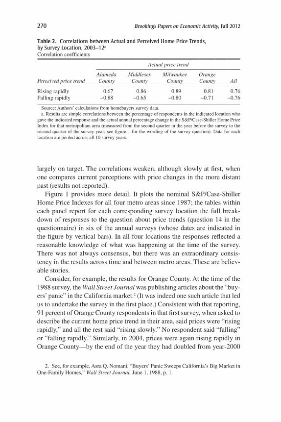
Table 2 compares the actual behavior of home prices in the four metro areas with what our respondents perceived to be happening in their area at the time. For each metro area across all 11 survey years, we calculated the correlation of the actual year-to-year change in the second-quarter aver-age of the local S&P/Case-Shiller Home Price Index with the percentage of respondents in the corresponding survey area in that year’s survey who said prices were “rising rapidly,” and with the percentage who said “falling rapidly.”1 If buyers were well informed, one would expect to see a high positive correlation of the year-over-year price increase with the percent-age saying “rising rapidly,” and a high but negative correlation with the percentage who said “falling rapidly.”

The simple correlation coefficients are indeed high in all four locations, and all have the right sign, indicating that respondents’ perceptions were

Table 1. response rates in the homebuyers survey, 1988–2012

Year Surveys returnedResponse rate

(percent)

1988 886 43.62003 705 35.32004 456 22.82005 441 22.12006 271 13.62007 300 15.02008 545 27.32009 370 18.52010 375 18.82011 319 16.02012 328 16.4All years 4,996 22.7

Source: Authors’ calculations from homebuyers survey data.

1. From question 14 of the questionnaire. The full questionnaire is available on the Brookings Papers website at www.brookings.edu/about/projects/bpea/, under “Past Editions.”


largely on target. The correlations weaken, although slowly at first, when one compares current perceptions with price changes in the more distant past (results not reported).

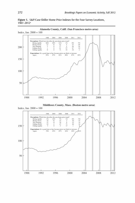
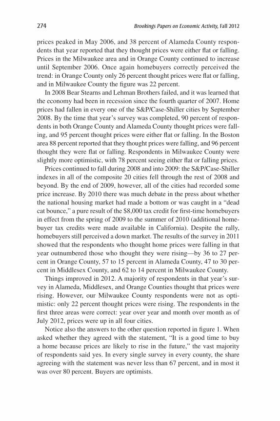
Figure 1 provides more detail. It plots the nominal S&P/Case-Shiller Home Price Indexes for all four metro areas since 1987; the tables within each panel report for each corresponding survey location the full break-down of responses to the question about price trends (question 14 in the questionnaire) in six of the annual surveys (whose dates are indicated in the figure by vertical bars). In all four locations the responses reflected a reasonable knowledge of what was happening at the time of the survey. There was not always consensus, but there was an extraordinary consis-tency in the results across time and between metro areas. These are believ-able stories.

Consider, for example, the results for Orange County. At the time of the 1988 survey, the Wall Street Journal was publishing articles about the “buy-ers’ panic” in the California market.2 (It was indeed one such article that led us to undertake the survey in the first place.) Consistent with that reporting, 91 percent of Orange County respondents in that first survey, when asked to describe the current home price trend in their area, said prices were “rising rapidly,” and all the rest said “rising slowly.” No respondent said “falling” or “falling rapidly.” Similarly, in 2004, prices were again rising rapidly in Orange County—by the end of the year they had doubled from year-2000

Table 2. correlations between actual and perceived home price trends, by survey location, 2003–12a

Correlation coefficients

Actual price trend

Perceived price trendAlameda County

Middlesex County

Milwaukee County

Orange County All

Rising rapidly 0.67 0.86 0.89 0.81 0.76Falling rapidly -0.88 -0.65 -0.80 -0.71 -0.76

Source: Authors’ calculations from homebuyers survey data.a. Results are simple correlations between the percentage of respondents in the indicated location who

gave the indicated response and the actual annual percentage change in the S&P/Case-Shiller Home Price Index for that metropolitan area (measured from the second quarter in the year before the survey to the second quarter of the survey year; see figure 1 for the wording of the survey question). Data for each location are pooled across all 10 survey years.

2. See, for example, Asra Q. Nomani, “Buyers’ Panic Sweeps California’s Big Market in One-Family Homes,” Wall Street Journal, June 1, 1988, p. 1.


levels—and respondents knew it: 100 percent said that home prices were rising rapidly (top right panel of figure 1). Homebuyers in Alameda County also correctly perceived the price trend in their metro area, that of San Francisco (top left panel of figure 1). In both California metro areas in both 1988 and 2004, fully 100 percent of respondents thought prices were rising.

Our Boston-area homebuyers, in contrast, saw a great deal of uncer-tainty in 1988. As the top right panel of figure 1 shows, the local market was at or approaching a peak in that year. It appears that people could not clearly see a trend amid the short-run noise: 37 percent of our Middlesex County respondents said prices were “not changing,” while most of the rest were split, with 34 percent saying prices were rising slowly and another 22 percent saying that they were falling slowly (bottom left panel of figure 1). Home prices in the Boston area were sticky and indeed essentially flat, but there was a great deal of debate at the time about the likelihood of a reces-sion and an actual price decline. Home prices in Milwaukee, by contrast, rose more slowly and steadily in the late 1980s (top right left panel of fig-ure 1), and our respondents’ perceptions reflect that. Like their Boston-area counterparts, few Milwaukee County respondents saw prices moving rap-idly in either direction: 53 percent perceived prices to be rising slowly, and another 24 percent said prices were not changing.

What we observed in the late 1980s was a set of housing markets behav-ing very differently across regions. By the middle of the 1990s, however, home prices in the United States had begun to move up in many markets at the same time. By 2000 the beginnings of a national boom were becoming evident. Between 2000 and 2005 the S&P/Case-Shiller 10-City compos-ite 10 index increased by more than 125 percent. Survey respondents in 2004 clearly saw the boom as it was occurring, In both California counties the vast majority said prices were rising rapidly, while in the Boston and Milwaukee areas most said prices were rising slowly.

The 2006 survey was sent out during a major turn in the marketplace. The boom ended sometime between late 2005 and early 2007, depending on the city, with home prices in Orange County up about 170 percent from their level in 2000. In San Francisco the increase from 2000 to the peak was 118 percent, and over the same period Boston was up 82 percent and Milwaukee 67 percent.

Finally the boom turned into a bust. The decline began in Boston, where prices peaked in September 2005. By the time the spring 2006 survey in the Boston area was tabulated, 70 percent of respondents were reporting that home prices were either not changing or falling. In San Francisco home


50

100

1988 1992 1996 2000 2004 2008 2012

150

200

Index, Jan. 2000 = 100Alameda County, Calif. (San Francisco metro area)

1988 2004 2006 2008 2011 2012

Perceptions: Which best describes the area home price trend?Rising rapidly 84% 69% 21% 1% 0% 5%Rising slowly 13 31 42 4 15 50Not changing 3 0 17 4 28 24Falling slowly 1 0 21 57 47 19Falling rapidly 0 0 0 33 10 2

Expectations: It's a good time to buy because prices are likely to increase. Agree 95% 87% 81% 80% 87% 85%

50

100

150

1988 1992 1996 2000 2004 2008 2012

Index, Jan. 2000 = 100Middlesex County, Mass. (Boston metro area)

1988 2004 2006 2008 2011 2012


Expectations: It's a good time to buy because prices are likely to increase.Agree 78% 83% 67% 82% 82% 81%

Figure 1. s&p/case-shiller home price indexes for the Four survey locations, 1987–2012a


50

100

150

200

250

1988 1992 1996 2000 2004 2008 2012

Index, Jan. 2000 = 100Orange County, Calif. (Los Angeles metro area)

1988 2004 2006 2008 2011 2012


Expectations: It's a good time to buy because prices are likely to increase.Agree 93% 72% 75% 79% 92% 86%

Sources: S&P/Case-Shiller and Fiserv, Inc. a. Vertical lines indicate quarters in which the homebuyers survey was conducted. The questions in

each table are from survey questions 14 and 25; the full survey questionnaire is available on the Brookings Papers website at www.brookings.edu/about/projects/bpea/, under “Past Editions."

1988 1992 1996 2000 2004 2008 2012

Index, Jan. 2000 = 100Milwaukee County, Wisc.

50

100

150

1988 2004 2006 2008 2011 2012


Expectations: It's a good time to buy because prices likely to increase.Agree 85% 83% 78% 85% 88% 89%

Figure 1. s&p/case-shiller home price indexes for the Four survey locations, 1987–2012a (Continued)


prices peaked in May 2006, and 38 percent of Alameda County respon-dents that year reported that they thought prices were either flat or falling. Prices in the Milwaukee area and in Orange County continued to increase until September 2006. Once again homebuyers correctly perceived the trend: in Orange County only 26 percent thought prices were flat or falling, and in Milwaukee County the figure was 22 percent.

In 2008 Bear Stearns and Lehman Brothers failed, and it was learned that the economy had been in recession since the fourth quarter of 2007. Home prices had fallen in every one of the S&P/Case-Shiller cities by September 2008. By the time that year’s survey was completed, 90 percent of respon-dents in both Orange County and Alameda County thought prices were fall-ing, and 95 percent thought prices were either flat or falling. In the Boston area 88 percent reported that they thought prices were falling, and 96 percent thought they were flat or falling. Respondents in Milwaukee County were slightly more optimistic, with 78 percent seeing either flat or falling prices.

Prices continued to fall during 2008 and into 2009: the S&P/Case-Shiller indexes in all of the composite 20 cities fell through the rest of 2008 and beyond. By the end of 2009, however, all of the cities had recorded some price increase. By 2010 there was much debate in the press about whether the national housing market had made a bottom or was caught in a “dead cat bounce,” a pure result of the $8,000 tax credit for first-time homebuyers in effect from the spring of 2009 to the summer of 2010 ( additional home-buyer tax credits were made available in California). Despite the rally, homebuyers still perceived a down market. The results of the survey in 2011 showed that the respondents who thought home prices were falling in that year outnumbered those who thought they were rising—by 36 to 27 per-cent in Orange County, 57 to 15 percent in Alameda County, 47 to 30 per-cent in Middlesex County, and 62 to 14 percent in Milwaukee County.

Things improved in 2012. A majority of respondents in that year’s sur-vey in Alameda, Middlesex, and Orange Counties thought that prices were rising. However, our Milwaukee County respondents were not as opti-mistic: only 22 percent thought prices were rising. The respondents in the first three areas were correct: year over year and month over month as of July 2012, prices were up in all four cities.

Notice also the answers to the other question reported in figure 1. When asked whether they agreed with the statement, “It is a good time to buy a home because prices are likely to rise in the future,” the vast majority of respondents said yes. In every single survey in every county, the share agreeing with the statement was never less than 67 percent, and in most it was over 80 percent. Buyers are optimists.


III. What Were Homebuyers’ Price Expectations for the Short and the Long Term?

Many stories of the housing boom in the early 2000s describe it as a bubble driven by irrational expectations. People are alleged to have been exces-sively optimistic. Our data allow us to examine such notions, as we began to do in our 2003 Brookings Paper, but now can do even better with the expectations data that our survey provides over the full course of the boom, bubble, and collapse.

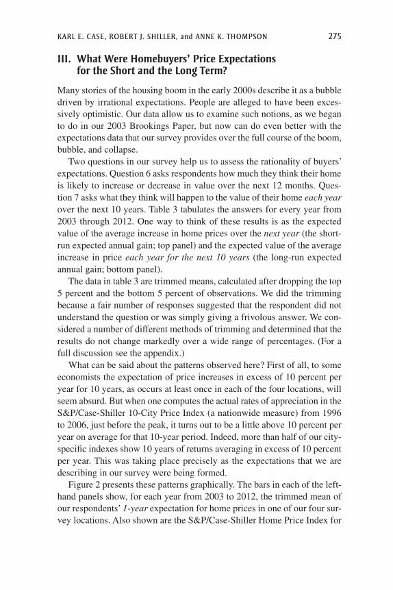
Two questions in our survey help us to assess the rationality of buyers’ expectations. Question 6 asks respondents how much they think their home is likely to increase or decrease in value over the next 12 months. Ques-tion 7 asks what they think will happen to the value of their home each year over the next 10 years. Table 3 tabulates the answers for every year from 2003 through 2012. One way to think of these results is as the expected value of the average increase in home prices over the next year (the short-run expected annual gain; top panel) and the expected value of the average increase in price each year for the next 10 years (the long-run expected annual gain; bottom panel).

The data in table 3 are trimmed means, calculated after dropping the top 5 percent and the bottom 5 percent of observations. We did the trimming because a fair number of responses suggested that the respondent did not understand the question or was simply giving a frivolous answer. We con-sidered a number of different methods of trimming and determined that the results do not change markedly over a wide range of percentages. (For a full discussion see the appendix.)

What can be said about the patterns observed here? First of all, to some economists the expectation of price increases in excess of 10 percent per year for 10 years, as occurs at least once in each of the four locations, will seem absurd. But when one computes the actual rates of appreciation in the S&P/Case-Shiller 10-City Price Index (a nationwide measure) from 1996 to 2006, just before the peak, it turns out to be a little above 10 percent per year on average for that 10-year period. Indeed, more than half of our city-specific indexes show 10 years of returns averaging in excess of 10 percent per year. This was taking place precisely as the expectations that we are describing in our survey were being formed.

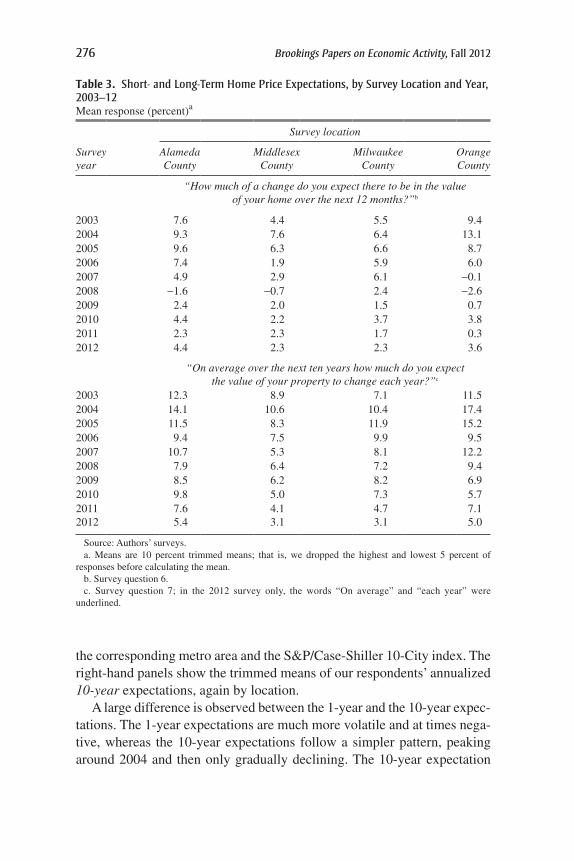
Figure 2 presents these patterns graphically. The bars in each of the left-hand panels show, for each year from 2003 to 2012, the trimmed mean of our respondents’ 1-year expectation for home prices in one of our four sur-vey locations. Also shown are the S&P/Case-Shiller Home Price Index for


Table 3. short- and long-term home price expectations, by survey location and Year, 2003–12 Mean response (percent)a

Survey location

Survey year

Alameda County

Middlesex County

Milwaukee County

Orange County

“How much of a change do you expect there to be in the value of your home over the next 12 months?”b

2003 7.6 4.4 5.5 9.42004 9.3 7.6 6.4 13.12005 9.6 6.3 6.6 8.72006 7.4 1.9 5.9 6.02007 4.9 2.9 6.1 -0.12008 -1.6 -0.7 2.4 -2.62009 2.4 2.0 1.5 0.72010 4.4 2.2 3.7 3.82011 2.3 2.3 1.7 0.32012 4.4 2.3 2.3 3.6

“On average over the next ten years how much do you expect the value of your property to change each year?”c

2003 12.3 8.9 7.1 11.52004 14.1 10.6 10.4 17.42005 11.5 8.3 11.9 15.22006 9.4 7.5 9.9 9.52007 10.7 5.3 8.1 12.22008 7.9 6.4 7.2 9.42009 8.5 6.2 8.2 6.92010 9.8 5.0 7.3 5.72011 7.6 4.1 4.7 7.12012 5.4 3.1 3.1 5.0

Source: Authors’ surveys.a. Means are 10 percent trimmed means; that is, we dropped the highest and lowest 5 percent of

responses before calculating the mean.b. Survey question 6.c. Survey question 7; in the 2012 survey only, the words “On average” and “each year” were

underlined.

the corresponding metro area and the S&P/Case-Shiller 10-City index. The right-hand panels show the trimmed means of our respondents’ annualized 10-year expectations, again by location.

A large difference is observed between the 1-year and the 10-year expec-tations. The 1-year expectations are much more volatile and at times nega-tive, whereas the 10-year expectations follow a simpler pattern, peaking around 2004 and then only gradually declining. The 10-year expectation

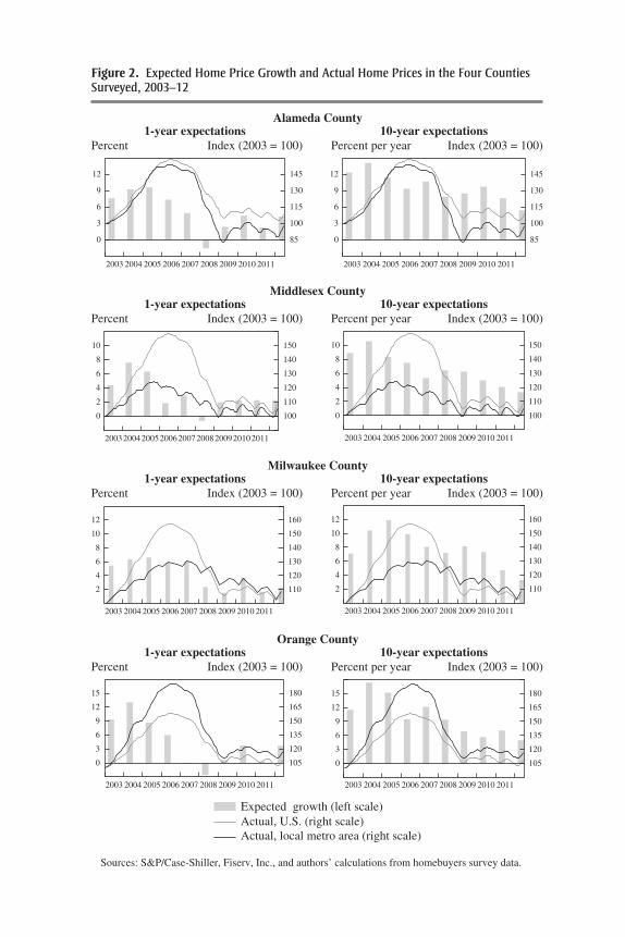
Figure 2. expected home price Growth and actual home prices in the Four counties surveyed, 2003–12

105

120

135

150

165

180

0

3

6

9

12

15

2004 2005 2006 2007 2008 2009 2010 20112003

105

120

135

150

165

180

0

3

6

9

12

15

2004 2005 2006 2007 2008 2009 2010 20112003

85

100

115

130

145

0

3

6

9

12

Percent Index (2003 = 100) Index (2003 = 100)Percent per year1-year expectations 10-year expectations

Alameda County

Middlesex County

Milwaukee County

Orange County




2004 2005 2006 2007 2008 2009 2010 20112003

100

110

120

130

140

150

0

2

4

6

8

10

2004 2005 2006 2007 2008 2009 2010 20112003

100

110

120

130

140

150

0

2

4

6

8

10

200420052006200720082009201020112003

2004 2005 2006 2007 2008 2009 2010 201120032004 2005 2006 2007 2008 2009 2010 20112003

110

120

130

140

150

160

2

4

6

8

10

12

85

100

115

130

145

0

3

6

9

12

2004 2005 2006 2007 2008 2009 2010 20112003

110

120

130

140

150

160

2

4

6

8

10

12

Expected growth (left scale)

Actual, local metro area (right scale)Actual, U.S. (right scale)

Sources: S&P/Case-Shiller, Fiserv, Inc., and authors’ calculations from homebuyers survey data.


exceeds the corresponding 1-year expectation in every year in every loca-tion, indicating that buyers are more optimistic about price increases over the long haul than in the short term.

Both kinds of expectations are important. If 1-year expectations are high, home sellers will have an incentive to wait another year to sell, while buyers will have an incentive to buy now rather than next year. But when it comes to the decision of whether to buy at all, and comparing the expected rate of return on the investment with the mortgage rate, the longer-term expectations are likely to be more important.

Table 4 presents yet another way of looking at the expectations data. Here we look at expectations since 2003, both short- and long-term, and at actual rates of change in nominal home prices annually from 1996 through 2012 for Orange (top panel) and Middlesex (bottom panel) Counties. This is important because later on we will consider how expectations reacted to changes taking place in the market.

The first column in the top panel of table 4 shows that in 2003, buyers in Orange County on average expected the value of their property to increase by 9.4 percent in the following year—well below the 18.2 percent increase in the previous year. When prices then jumped 31.1 percent between 2003 and 2004, it must have been a surprise. Similarly, in 2004 buyers expected prices to increase 13.1 percent in the year following their purchase, but in fact prices rose 18.5 percent. A similar pattern can be observed in the Boston area (bottom panel), but the expected and actual rates of change are lower.

When asked to project how much their home’s value would increase or decrease in each of the following 10 years, homebuyers in both locations were more optimistic. But even these expectations were not unreasonable given the performance of the market before 2006. Price increases in Orange County were actually accelerating after 2000, and long-term expectations remained solid as long as prices continued to rise. Even when prices started falling sharply in 2007 and 2008, buyers continued to expect healthy price appreciation over the next 10 years, and even their 1-year expectations resisted the idea that the severe drops that were already occurring would continue.

IV. Were Homebuyers’ Expectations Rational and How Were They Formed?

We can test whether the expectations of our homebuyers were rational by regressing actual home price changes on the expected changes. Of course, with our present data set we can do this only for the 1-year expectations,


Table 4. expected versus actual short- and long-term home price expectations in orange and middlesex counties

Survey location and year

Expected annual price increase (percent) Actual

1-year price increase (percent)

Implied value of a home worth

$100,000 in 1996Next year

Next 10 years

Orange County1996 n.a.a n.a. $100,0001997 n.a. n.a. 2.4 102,4401998 n.a. n.a. 12.8 115,5941999 n.a. n.a. 11.5 128,9022000 n.a. n.a. 10.2 142,0742001 n.a. n.a. 9.8 155,9862002 n.a. n.a. 11.8 174,3182003 9.4 11.5 18.2 206,0432004 13.1 17.4 31.1 270,2052005 8.7 15.2 18.5 320,1672006 6.0 9.5 14.9 367,8832007 -0.1 12.2 -3.3 355,6622008 -2.6 9.4 -24.3 269,0822009 0.7 6.9 -19.6 216,2122010 3.8 5.7 8.9 235,4502011 0.3 7.1 -2.9 228,5952012 3.6 5.0 -2.1 223,901

Middlesex County1996 n.a. n.a. $100,0001997 n.a. n.a. 6.0 105,9621998 n.a. n.a. 8.8 115,2981999 n.a. n.a. 12.3 129,4972000 n.a. n.a. 14.1 147,8102001 n.a. n.a. 16.4 172,0902002 n.a. n.a. 10.8 190,6552003 4.4 8.9 11.3 212,1612004 7.6 10.6 9.6 232,4432005 6.3 8.3 8.4 252,0312006 1.9 7.5 -1.4 248,5832007 2.9 5.3 -4.2 238,2182008 -0.7 6.4 -6.0 224,0012009 2.0 6.2 -6.9 208,4462010 2.2 5.0 4.3 217,4992011 2.3 4.1 -3.2 210,5512012 2.3 3.1 0.0 210,476

Sources: S&P/Case-Shiller, Fiserv, Inc., and authors’ calculations from homebuyers survey data.a. n.a. = not available.


since we do not have 10 years of subsequent price data. The majority of the surveys in each year were returned in the second quarter, so we calculated the actual price change in each metro area as the percentage change in the S&P/Case-Shiller Home Price Index for that area from one second quarter to the next. Under traditional rational expectations theory, the constant term in these regressions should be zero, and the slope coefficient should equal +1. The top panel of table 5 reports the results. In all four survey locations the slope coefficients are statistically significant and have the right sign, but they are always much greater than 1. (The constant term is always negative, reflecting a necessary correction for the mean when the slope coefficient is greater than 1.) This may be interpreted as implying that home owners had information that was relevant to the forecast but were not aggressive enough in their forecasts. A scatter diagram of actual against expected 1-year price changes for the four metro areas (figure 3) conveys how far individuals underestimated the absolute magnitude of home price movements.

Table 5. regressions testing for rational expectations of the one-Year change in home pricesa

Survey location

Alameda County

Middlesex County

Milwaukee County

Orange County All

Using S&P/Case-Shiller Home Price Indexes, 2003–12Constant -12.79 -4.75 -5.67 -9.48 -9.13

(8.84) (2.85) (4.52) (5.16) (2.52)Own-city expected

12-month price changeb

2.57(1.42)

1.50(0.71)

1.43(0.94)

2.71(0.78)

2.34(0.46)

No. of observations 9 9 9 9 36R2 0.32 0.39 0.25 0.63 0.43

Using FHFA home price dataConstant -8.60 -4.82 -6.96 -8.75 -8.11

(4.12) (2.50) (3.45) (2.88) (1.48)Own-city expected

12-month price changeb

2.03(0.66)

1.73(0.62)

1.86(0.72)

2.81(0.44)

2.32(0.27)


Sources: Authors’ regressions using data from S&P/Case-Shiller, Fiserv, Inc., the Federal Housing Finance Agency, and the homebuyers survey.

a. Each column in each panel reports results of a single regression. The dependent variable is the actual percentage home price change in the indicated city from the second quarter of the year to the second quarter of the following year. Standard errors are in parentheses.

b. Trimmed mean of responses to question 6 of the homebuyers survey.


–20

–10

0

20

10

30

3020100–10–20

Alameda

Actual changeb (percent)

Expected change (percent)c

Middlesex

Milwaukee

Orange

Source: S&P/Case-Shiller, Fiserv, Inc., and authors’ calculations from survey data. a. Each observation represents one of the four survey locations in a single year. b. Actual change in metro-area home prices from the second quarter of the survey year to the second

quarter of the next year.c. Trimmed mean of respondents’ expected change in home prices for the next year.

Figure 3. expected versus actual one-Year changes in home prices, 2003–11a

Contrary to what one might expect from popular stories about bubble mentality, then, the 1-year expectations of homebuyers were not over-reacting to information, but rather underreacting to it. However, this is not necessarily inconsistent with the presence of a bubble. Certainly, the longer-term expectations, whose rationality is harder to judge, seem likely to have been more in line with information in the early years of our sam-ple when they were predicting appreciation of over 10 percent a year for the next 10 years.

The above results do not depend on using the S&P/Case-Shiller Home Price Indexes to measure actual price changes. Substituting the home price indexes of the Federal Housing Finance Agency (FHFA, formerly the Office of Federal Housing Enterprise Oversight, OFHEO) yields rather similar results (bottom panel of table 5). Unlike the S&P/Case-Shiller indexes, the FHFA indexes include appraised values as well as actual sales in their construction.

Much of this apparent underreaction of expectations to information about future home prices is confined to certain metro areas and episodes. Note that in the metro areas where prices were tamer, Milwaukee and Boston, the coefficients in table 5 using the S&P/Case-Shiller data are 1.50


or less and not statistically significantly different from 1; although the coef-ficients are slightly higher in the regressions using the FHFA data, they still are not significantly different from 1.

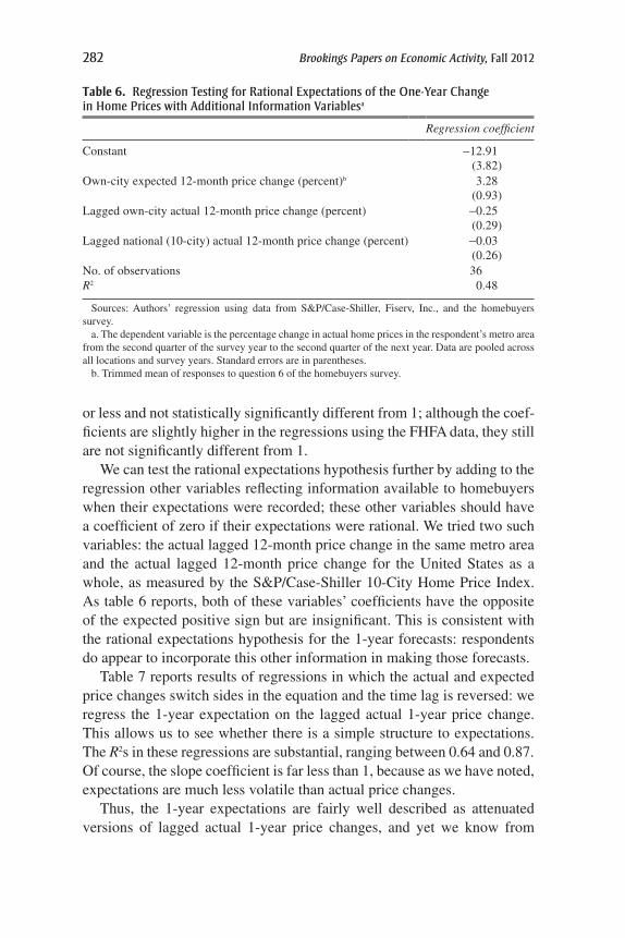
We can test the rational expectations hypothesis further by adding to the regression other variables reflecting information available to homebuyers when their expectations were recorded; these other variables should have a coefficient of zero if their expectations were rational. We tried two such variables: the actual lagged 12-month price change in the same metro area and the actual lagged 12-month price change for the United States as a whole, as measured by the S&P/Case-Shiller 10-City Home Price Index. As table 6 reports, both of these variables’ coefficients have the opposite of the expected positive sign but are insignificant. This is consistent with the rational expectations hypothesis for the 1-year forecasts: respondents do appear to incorporate this other information in making those forecasts.

Table 7 reports results of regressions in which the actual and expected price changes switch sides in the equation and the time lag is reversed: we regress the 1-year expectation on the lagged actual 1-year price change. This allows us to see whether there is a simple structure to expectations. The R2s in these regressions are substantial, ranging between 0.64 and 0.87. Of course, the slope coefficient is far less than 1, because as we have noted, expectations are much less volatile than actual price changes.

Thus, the 1-year expectations are fairly well described as attenuated versions of lagged actual 1-year price changes, and yet we know from

Table 6. regression testing for rational expectations of the one-Year change in home prices with additional information Variablesa

Regression coefficient

Constant -12.91(3.82)

Own-city expected 12-month price change (percent)b 3.28(0.93)

Lagged own-city actual 12-month price change (percent) -0.25(0.29)

Lagged national (10-city) actual 12-month price change (percent) -0.03(0.26)

No. of observations 36R2 0.48

Sources: Authors’ regression using data from S&P/Case-Shiller, Fiserv, Inc., and the homebuyers survey.

a. The dependent variable is the percentage change in actual home prices in the respondent’s metro area from the second quarter of the survey year to the second quarter of the next year. Data are pooled across all locations and survey years. Standard errors are in parentheses.

b. Trimmed mean of responses to question 6 of the homebuyers survey.


table 6 that they also contain significant information about future price changes beyond what is contained in the lagged actual price change. This conclusion does not mean, however, that any story of feedback in deter-mining price should be modeled in rational terms. Long-term expectations also matter importantly for demand for housing, because as previously noted, they are important to people’s decisions about whether to buy a home at all.

As John Maynard Keynes suggested in his 1936 General Theory of Employment, Interest and Money, it is long-term expectations that may be the real driver of speculative booms, even though these expectations are not normally the focus of economic forecasters. It may be a general expec-tation about the vague and distant future that helps explain why people behaved in the 2000s as if they thought that home prices could never fall: perhaps they thought so only about the long run, as our 10-year expecta-tions data seem to confirm.

Figure 4 shows annualized 10-year expectations of home price appre-ciation from our survey, averaged across our four locations, along with the national-average 30-year mortgage rate, from 2003 to 2012. These two series are roughly matched in term, since the average actual duration of a mortgage in the United States, before a move or a refinancing or the like, is about 7½ years, not the contractual 30 years. As the figure shows, these expectations, if they could have been trusted, implied enormous profit opportunities in buying a home around 2004: the spread between the two series was roughly 6 percentage points. Leveraging their investment 10 to 1

Table 7. regressions of the expected one-Year change in home prices on lagged actual price changesa

Survey location

Alameda County

Middlesex County

Milwaukee County

Orange County Allb

Constant 4.87 2.79 3.76 3.25 3.72(0.64) (0.49) (0.30) (0.61) (0.28)

Lagged own-city actual 12-month price change (percent)

0.18(0.04)

0.29(0.07)

0.30(0.05)

0.26(0.04)

0.23(0.02)


Sources: Authors’ regressions using data from S&P/Case-Shiller, Fiserv, Inc., and the homebuyers survey.

a. Each column reports results of a single regression. The dependent variable is the trimmed mean of the expected 1-year change in home prices in the indicated location. Standard errors are in parentheses.

b. Data are pooled across all locations and survey years.


(as one does when taking out a standard conventional mortgage), our home-buyers in 2004 would have expected to multiply that 6-percentage-point spread by 10 (after taking the other expenses of homeownership into account). This helps explain the bubble enthusiasm of that time.

After 2004, however, long-term expectations fell faster than mortgage rates, so that this expected profit opportunity narrowed, sharply at first and then more gradually. Neither monetary stimulus nor the other policy measures applied in the wake of the financial crisis—neither lower inter-est rates, the federal conservatorship of Fannie Mae and Freddie Mac, the Public-Private Investment Program, quantitative easing, nor Operation Twist—succeeded in lowering mortgage interest rates by anything like the decline in expectations.

By 2012, as figure 4 shows, long-term expectations had fallen to a level practically equal to the mortgage rate, suggesting that homebuyers no lon-ger perceived a long-term profit opportunity in investing in a home. Since a sample consisting only of homebuyers is likely to be upwardly biased in terms of expectations relative to the population as a whole, the perceived investment opportunity among the general population may be even lower. A survey of professional forecasters conducted by Pulsenomics LLC sug-gests that these professionals are less optimistic than our respondents.

2

4

6

8

10

12

2003 2004 2005 2006

Percent per year

2007 2008 2009 2010 2011 2012

Expected 10-year change in home prices (annualized)a

30-year mortgage rate

Sources: Freddie Mac’s Primary Mortgage Market Survey and authors’ calculations from survey data. a. Average of trimmed means for all survey respondents.

Figure 4. ten-Year expectations for home price Growth and thirty-Year mortgage rates, 2003–12


Their average expectation for annual home price appreciation for 2012–16, reported in the June 2012 Pulsenomics survey, was 1.94 percent, about half the 10-year expectation of the homebuyers in our 2012 survey.

Why were home price expectations so high relative to interest rates around 2004? Some simple stories come to mind but cannot be proved or disproved with any data that we know of. One is that these long-term expectations were formed over many decades during which home prices more or less consistently rose. Another is that money illusion plays a role: people may fail to consider that with lower overall inflation today than in past decades, home price increases are likely to be smaller than in the past.

Notably, the peak in expectations during the 2000s boom occurred 2 years before prices began to fall, 3 years before the beginnings of the subprime crisis, and 4 years before the most intense phase of the crisis in late 2008. This, together with the fact that the decline in expectations is fairly steadily downward over the 8 years after 2004, shows that the crisis cannot be the cause. Perhaps that should not be altogether surprising, for the crisis was presented to the public as just that—something short-term. It was associated with an economic recession, and all recessions in recent decades have been short. So perhaps it was not so much the crisis itself as its surprising duration that gradually contributed to bringing expectations further down.

V. How Did the Bubble End?

Our sample period includes only one major turning point in the housing market, the sudden, historic end of the housing bubble. Although we have only one observation of this turning point, understanding it is central to our objectives. Of particular interest here are respondents’ answers to a pair of open-ended questions in the survey (questions 16 and 17):

—Was there any event or events in the last two years that you think changed the trend in home prices?

—What do you think explains recent changes in housing prices in [location]? What, ultimately is behind what is going on?

Most respondents wrote in answers to these questions; only a few left them blank. The questionnaires left space for writing 20 words or so, and many filled the available space. Only a few wrote one-word answers.

Comparing the responses to these two questions between the 2004 and 2006 surveys seems likely to be fruitful for understanding the turning point, because long-term expectations dropped a full 4 percentage points over that relatively short interval, roughly half of the total drop from the


peak. Moreover, the answers will not be clouded by any references to the financial crisis, which was still entirely in the future.

Between these two years, a striking change in the tenor of the answers can be observed. The common themes in 2004 included a “shortage of houses,” a large number of “immigrants,” “scarcity of land,” “lack of building space,” “too many people,” and “the desire to have it all.” These answers are mostly consistent with perceptions of a shortage of supply. Only occasionally did respondents mention in 2004 that affordability might be an issue. By 2006 the optimistic themes of 2004 were still in evidence but were less prevalent. The most common theme in 2006 was “rising inter-est rates.” Some themes were mentioned repeatedly, in different forms, as suggested by answers such as the following: “high prices,” “no equivalent rise in wages,” “overvalued homes,” “numerous newspaper & media arti-cles speculating on/or reporting on slowing sales,” and “astronomical price spikes of previous 2 years simply cannot be sustained.”

In 2004, 14 percent of respondents volunteered the word “supply” in answering these two questions, almost always with a suggestion of short supply, limited supply, no supply, or demand exceeding supply. In 2006 only 5 percent of respondents used this word.

As figure 5 shows, the phrase “housing bubble” did not appear in a single handwritten response in 2004, although one respondent used the

0.5

1.0

1.5

2.0

2.5

3.0

2003 2004 2005 2006 2007 2008 2009 2010 2011 2012

Source: Authors’ calculations from homebuyers survey data. a. Share of respondents who used the words “housing bubble” anywhere in their answers to the

homebuyers survey.

Percent of responses

Figure 5. appearances of “housing bubble” in homebuyers survey responses, 2003–12a


term in 2003. By 2006, however, the word was being volunteered by a few respondents. As time went on after the crisis, the percentage mentioning “housing bubble” rose, until by 2010 over 3 percent of the respondents were using the term.

As of 2004, a few professional economists were already responding to the claim of some that the housing market was in a bubble. Our own 2003 Brookings Paper (Case and Shiller 2003) strongly suggested that housing was in a bubble, but others took a different view.

Our questionnaire itself did not use the word “bubble” except in the 2010 survey, when we added the following yes-or-no question:3

Do you think the home price boom and bust in first decade of the 2000s was basically a speculative bubble and burst (prices driven up by greed and excessive speculation and then inevitably collapsing down)?

Eighty-five percent of respondents answered yes to this question. It is too bad that we did not think to ask this question until 2010. We probably did not in 2003 or 2004 because we could not have then imagined that many people would even recognize the term “speculative bubble” in this context.

There was a clear change in public perceptions in the 2 years between 2004 and 2006. Ideas (speculative bubbles, overpriced homes) that were “in the air” in 2004 actually were not much talked about then, but their frequency of mention had increased dramatically by 2006.

Why was there such a dramatic increase in these notions? Between 2004 and 2006, the idea seems to have emerged in media accounts that there are such things as bubbles and that they might be expected to burst. Over this 2-year period, a number of analyses of bubble arguments appeared, most of them in publications that few homeowners are likely to have read. They must have viewed the news accounts of these debates more as a sporting event, whose outcome was very uncertain.

In December 2004 Joseph McCarthy and Richard Peach published an article in the Federal Reserve Bank of New York’s Economic Policy Review, “Are Home Prices the Next Bubble?” in which they answered their title question in the negative. They argued that home prices might not even have increased at all, if one adjusted for quality changes: a repeat-sales index like the OFHEO index (or the Case-Shiller index) may not effectively control for quality if homeowners improve their homes between sales. However, the only evidence they offered for a widespread change in

3. In this year as in some others, we added one or more questions at the end of the ques-tionnaire, without, however, changing the wording of any of the other questions.


average home quality was that the overall increase in the OFHEO index in recent years was approximately the same as that of the ordinary median price, which does not attempt to hold quality constant.

In February 2005 David Lereah published his book Are You Missing the Real Estate Boom? Lereah strongly rejected the mounting suspicion that a real estate bubble was forming. He argued instead that lower interest rates meant that housing was much more affordable than it had been in the previous couple of decades, and that demand from the baby-boom genera-tion would keep the market going strong for years to come. Although he was right about these points, it was still a leap of judgment to conclude, as he did, that the housing market at the time offered a “once-in-every-other generation opportunity” for investors.

In March 2005 one of us (Shiller) published the second edition of his book Irrational Exuberance, which included a new data set on real home prices since 1890. No such long data set of U.S. home prices had ever been published before, and a chart depicting the aggregate series revealed that by historical standards the current real estate boom was highly abnormal, “like a rocket taking off” (Shiller 2005, p. 4). The chart was reprinted in a number of places, including the New York Times.

On June 16, 2005, the Economist published a cover story titled “After the Fall,” with a cover illustration of a falling brick inscribed with the words “house prices.” The story said:

Perhaps the best evidence that America’s house prices have reached dangerous levels is the fact that house-buying mania has been plastered on the front of virtu-ally every American newspaper and magazine over the past month. Such bubble-talk hardly comes as a surprise to our readers. We have been warning for some time that the price of housing was rising at an alarming rate all around the globe, including in America. Now that others have noticed as well, the day of reckoning is closer at hand. It is not going to be pretty. How the current housing boom ends could decide the course of the entire world economy over the next few years.4

Indeed, it does appear that the news media had by this time flocked to the notion that the housing boom was really a bubble. On June 13, 2005, Time published a cover story titled “Why We’re Going Gaga over Real Estate,” with an illustration of a man lovingly hugging a house. A week later Barron’s ran a cover story by Jonathan Laing titled “The Bubble’s New Home.”

Why did all this media attention happen so suddenly? It is hardly controversial to suggest that the major news media are always looking

4. The Economist, “After the Fall,” June 16, 2005. www.economist.com/node/4079458.


for stories that will resonate with their readers, and that when one of them comes across such a story, the others follow. Somehow the housing bubble story seems to have become such a story around that time, mark-ing a turning point in public thinking. That people were changing their thinking about housing bubbles in mid-2005 can also be measured by a Google Trends count of web searches for the term “housing bubble.” As figure 6 shows, 2005 saw a sudden burst in web searches for this term, peaking in August.

Fernando Ferreira and Joseph Gyourko (2011) find a wide dispersion in the timing of the beginning of the real estate bubble, ranging from 1994 in some metro areas to 2005 in others. But their analysis also shows that all this came to an abrupt end in all areas at about the same time, just before 2006. Even many months after public opinion had begun to turn decisively toward the view that the recent boom in home prices was a bubble, some economists continued to argue that all price increases were justified by fundamentals and that there was no bubble.

In March 2006 Margaret Hwang Smith and Gary Smith presented a paper before the Brookings Panel that argued, among other things, that the downtrend in nominal interest rates since 2000 fully justified the increase in home prices. One of us argued, in a comment on their paper (Shiller 2006),

20

10

30

50

70

90

2004 2005 2006 2007 2008 2009 2010 2011 2012

40

60

80

Source: Google Trends (www.google.com/trends/?q=housing+bubble). Accessed January 1, 2013.

August 14–20, 2005 (peak) = 100

Figure 6. Google Web searches for “housing bubble,” january 4, 2004, to september 9, 2012


that whether speculative price changes are “justified” can be answered in many ways and that the issues in financial theory are sufficiently complex that it is hard to be definitive, yet that there were reasons to suspect that the observed price changes were related to swings in public opinion rather than changes in fundamentals.

Smith and Smith (2006) is, to our knowledge, the last major paper to argue that there never was a housing bubble in the 2000s. By 2006 a sub-stantial segment of the population had concluded that it was a bubble, and professional economists as apologists largely disappeared.

VI. What Caused the Rebound in 2009–10 and Why Did It Fizzle?

The rebound in home prices from 2009 to 2010 is quite striking. In some metro areas it was strong: San Francisco–area home prices rose 22 percent in the 16 months between March 2006 and July 2010 (see top left panel of figure 1). But this rebound did not last, and home prices resumed their fall. Interestingly, long-term expectations for home prices did not increase between 2009 and 2010. What, then, might explain the temporary uptick?

It is at first striking that very few respondents’ answers to our open-ended questions about the forces behind home price trends even mention the “usual suspects” that economists would consider. In none of the almost 2,000 questionnaires returned from 2008 to the present is there a single mention of the Home Affordable Modification Program (HAMP, created by the Emer-gency Economic Stabilization Act of 2008 and amended by the American Recovery and Reinvestment Act of 2009), the Home Affordable Refinanc-ing Program (HARP), or the Homeowners Affordability and Stability Plan (HASP, announced by President Barack Obama in February 2009, using funds from the Housing and Economic Recovery Act of 2008). Nor did any-one mention either of Fannie Mae’s refinancing programs Refi Plus and DU Refi Plus. This whole alphabet soup of relatively ineffective homeowner assistance programs appears to have been totally missed by our respondents, although some of their answers may have included vague, hard-to-interpret references to them or their effects.

The homebuyer tax credit, created by the American Recovery and Reinvestment Act in February 2009, the second month of President Obama’s tenure, was much more salient, perhaps because it took the form of a substantial outright gift to eligible parties: initially these were first-time homebuyers, who received a credit of up to $8,000, but later other homebuyers were granted a credit of as much as $6,500. The credit’s


expiration date, originally November 30, 2009, was later extended to April 30, 2010 (with closing required by June 30), when non-first-time buyers were also allowed.5 The total cost of the program was estimated at $22 billion.6

The fact that these tax credits came at the beginning of a new presi-dency, at a time when other stimulus programs were being announced, may have amplified the sense of hope that they offered. A search through our questionnaires for the words “tax credit” produced 3 hits in 2009, 37 in 2010, 10 in 2011, and 2 in 2012. In 2010 all but one of the 37 men-tions came from first-time homebuyers. The questionnaire for 2010 dif-fered from those in all other years in that it asked (question 22b, well after questions 16 and 17), “Are you getting the home buyer tax credit for this home purchase?” This may have reminded some respondents (who did not necessarily answer all questions in order) of this fact and prompted them to mention the credit in the earlier questions.

A remarkably large fraction of respondents in 2010—80 percent in Orange County, 65 percent in Middlesex and Milwaukee Counties, and 64 percent in Alameda County—said that they would receive the credit. The credit appears to have motivated some households to become home-owners: figure 7 shows that the fraction of our respondents who were first-time homebuyers rose to 53 percent in 2009, compared with 42 per-cent in 2008 and 34 percent in 2006.

These results suggest that the homebuyer tax credit was an important factor in the temporary turnaround in the housing market: homebuyers were aware of it, leading sales and prices to increase and inventory (as measured by months of supply, from the National Association of Realtors) to fall. This set the stage for a decline in home prices in 2011, possibly unrelated to expectations of future price increases.

5. A $7,500 tax credit was also legislated as part of the Housing and Economic Recovery Act of 2008, but that credit had to be repaid and so was really a loan rather than a subsidy.

6. U.S. Government Accountability Office, in a letter to Rep. John Lewis (D-Ga.), chair-man of the House Subcommittee on Oversight, September 2, 2010 (www.gao.gov/new.items/d101025r.pdf). Since two of our four survey locations are in California, it is worth noting that California had its own homebuyer tax credits, each worth $10,000. The first was in effect from March 1, 2009, to February 28, 2010. It was not limited to first-time buyers but was limited to newly built homes. The second, in effect between May 1, 2010, and December 31, 2010, allocated $100 million to first-time homebuyers and an additional $100 million to other purchasers of new homes. Both credits were distributed on a first-come, first-served basis. Measured on a per capita basis, the California program was less than a tenth the size of the federal program.


A couple of theories come to mind to explain why homebuyers sud-denly came into the market just then. One theory is that the decisive gov-ernment action in legislating the tax credit persuaded them that home prices would quickly go up. But this theory is belied by our expectations data in figure 2. Short-term expectations generally improved between 2008 and 2009 or 2010, but not by much, and so remained low by histori-cal standards. Nor did long-term expectations change much between 2008 and 2009 or 2010.

Another possible explanation relies on the psychological theory of regret. The homebuyer tax credit was a reason for homebuyers to act quickly. Missing the credit, and perhaps buying soon after it expired, would generate a pang of regret. Regret theory, as advanced by Graham Loomis and Robert Sugden (1982), argues that people are especially motivated to avoid the feeling of regret for having missed an opportunity or made a mis-take, and that the regret itself looms large in their mind, sometimes out of proportion to the actual loss.

To the extent that regret theory explains the market impact of the homebuyers tax credit on home prices, it might also help explain why the 2009–10 rally fizzled. These dates do not mark a substantial upward turn-

10

20

30

40

50

Percenta

2003 2004 2005 2006 2007 2008 2009 2010 2011 2012

Source: Authors’ calculations from homebuyers survey data. a. Percent of respondents answering “yes” to question 4 of the survey: “Are you a first time home

buyer?”

Figure 7. First-time buyers in the homebuyers survey, 2003–12


ing point as did 2004–06 because there was no fundamental change in expectations.

VII. Conclusion

The rise and fall of the housing market during the past decade is one of the most important events in modern economic history. This paper has focused on a factor in that episode that has received little formal analysis: the role of expectations. We have tried to draw some conclusions from a data set of nearly 5,000 completed mail questionnaires collected over the past 25 years from actual homebuyers in four metropolitan areas.

The descriptions of the data and the questions that we ask may seem somewhat ad hoc and arbitrary, but as we noted at the outset, no theo-retical framework exists to guide us. However, we can say a few things in conclusion. First, the data suggest that homebuyers were very much aware of trends in home prices at the time they made their purchase. There is a strong correlation between the respondents’ stated perceptions of price trends and actual movements in prices. The data also show that the opinions of homebuyers have varied over time. When price trends are strong, there is little disagreement among respondents. When there is ambiguity, respondents seem, not surprisingly, to have a much less clear picture.

The data also show that homebuyers were, if anything, out in front of the short-term changes that were occurring and that their short-run expecta-tions underreacted to the year-to-year changes in actual home prices. Their long-term expectations have been consistently more optimistic across both time and locations, but the absolute difference between long-term and short-term expectations fell from a high of 8.3 percentage points in 2008 to just 0.8 percentage point in 2012. We cannot test the rationality of long-term expectations as we can the short-term expectations, and yet, since most homebuyers own their home for many years, these are arguably the more important determinants of housing demand. It is from these nebulous and relatively slow-moving expectations that the bubble took much of its impetus, and that future home price movements will as well.

Perceptions of where prices are headed in the short term turned more positive in 2012, but long-term expectations continued to weaken. Thus, although a recovery may be plausible, and home prices were rising fairly strongly as this paper went to press, we do not see any unambiguous indi-cation in our expectations data of the sharp upward turnabout in demand for housing that some observers and media accounts have suggested.


a p p e n d i x

Controlling for Outliers

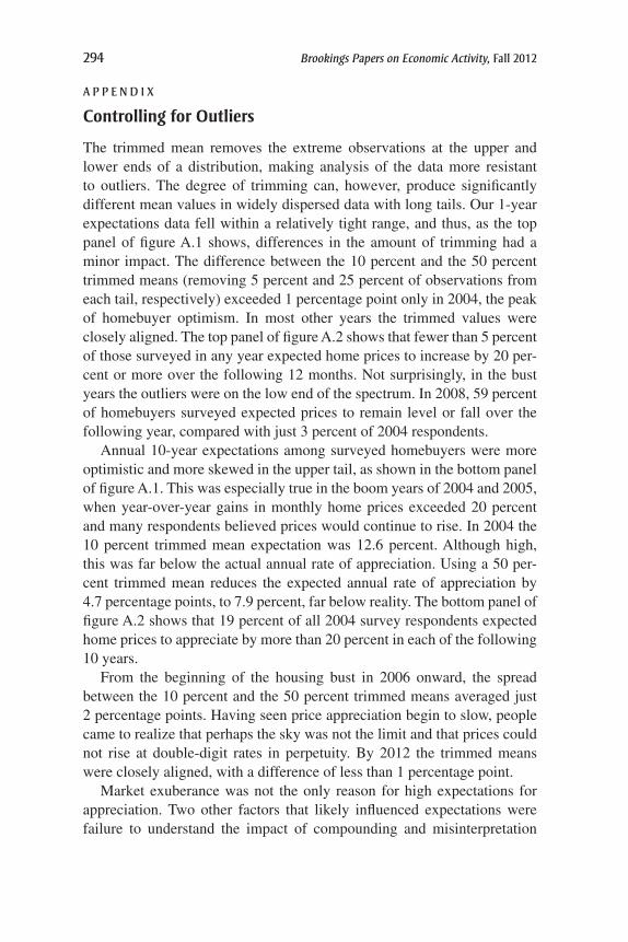
The trimmed mean removes the extreme observations at the upper and lower ends of a distribution, making analysis of the data more resistant to outliers. The degree of trimming can, however, produce significantly different mean values in widely dispersed data with long tails. Our 1-year expectations data fell within a relatively tight range, and thus, as the top panel of figure A.1 shows, differences in the amount of trimming had a minor impact. The difference between the 10 percent and the 50 percent trimmed means (removing 5 percent and 25 percent of observations from each tail, respectively) exceeded 1 percentage point only in 2004, the peak of homebuyer optimism. In most other years the trimmed values were closely aligned. The top panel of figure A.2 shows that fewer than 5 percent of those surveyed in any year expected home prices to increase by 20 per-cent or more over the following 12 months. Not surprisingly, in the bust years the outliers were on the low end of the spectrum. In 2008, 59 percent of homebuyers surveyed expected prices to remain level or fall over the following year, compared with just 3 percent of 2004 respondents.

Annual 10-year expectations among surveyed homebuyers were more optimistic and more skewed in the upper tail, as shown in the bottom panel of figure A.1. This was especially true in the boom years of 2004 and 2005, when year-over-year gains in monthly home prices exceeded 20 percent and many respondents believed prices would continue to rise. In 2004 the 10 percent trimmed mean expectation was 12.6 percent. Although high, this was far below the actual annual rate of appreciation. Using a 50 per-cent trimmed mean reduces the expected annual rate of appreciation by 4.7 percentage points, to 7.9 percent, far below reality. The bottom panel of figure A.2 shows that 19 percent of all 2004 survey respondents expected home prices to appreciate by more than 20 percent in each of the following 10 years.

From the beginning of the housing bust in 2006 onward, the spread between the 10 percent and the 50 percent trimmed means averaged just 2 percentage points. Having seen price appreciation begin to slow, people came to realize that perhaps the sky was not the limit and that prices could not rise at double-digit rates in perpetuity. By 2012 the trimmed means were closely aligned, with a difference of less than 1 percentage point.

Market exuberance was not the only reason for high expectations for appreciation. Two other factors that likely influenced expectations were failure to understand the impact of compounding and misinterpretation


0

2

4

6

8

10

12

2003 2004 2005 2006 2007 2008 2009 2010 2011 2012

One-year expectations

Ten-year expectations (annualized)

Percent

Percent per year

Trimmed 10%Trimmed 15%Trimmed 20%Trimmed 50%Median

Trimmed 10%Trimmed 15%Trimmed 20%Trimmed 50%Median

30-year mortgage rate

0

2

4

6

8

10

12

2003 2004 2005 2006 2007 2008 2009 2010 2011 2012

Sources: Freddie Mac’s Primary Mortgage Market Survey and authors’ calculations from homebuyers survey data.

Figure A.1. expected home price Growth Using alternative trimmings of outliers, 2003–12


of the question on long-term expectations. For example, a survey respon-dent who expects prices to double over the next decade might mistakenly report an expected annual increase of 10 percent. In fact, a compound 10 percent annual increase would bring the price of a $100,000 home to $285,000 over 10 years, not $200,000. Some of those surveyed also appeared to misinterpret the question as the total appreciation over the next 10 years, not the annual rate of appreciation. This is likely the case among

10

20

30

40

50

60

70

80

90

2003 2004 2005 2006 2007 2008 2009 2010 2011 2012

One-year expectations

Ten-year expectations (annualized)

Percent of respondents

Percent of respondents

10

20

30

40

50

60

70

80

90

2003 2004 2005 2006 2007 2008 2009 2010 2011 2012

Expectedgrowth g (%) g > 20 10 < g ≤ 20 5 < g ≤ 10 0 < g ≤ 5 g ≤ 0

Expectedgrowth g (%) g > 20 10 < g ≤ 20 5 < g ≤ 10 0 < g ≤ 5 g ≤ 0

Source: Authors’ calculations from homebuyers survey data.

Figure A.2. distributions of expected one-Year and ten-Year home price Growth


those respondents who reported their 10-year annual expected appreciation as 10 times their 1-year expectation.

Questions have been added to the end of the survey questionnaire in the past, and more will likely be added in the future as we continue to assess what important additional information we might garner from respon-dents. A second long-term expectations question, “How much higher do you expect home prices to be, in percentage terms, in 10 years?” might yield interesting results. However, we would expect to find some appar-ent inconsistencies between the answers to this question and the answers to the question about expected annual appreciation for 10 years, and we still would not know which question elicited their true 10-year expectation. Most people are not used to making 10-year forecasts and have trouble knowing whether prices might double or triple or anything else. We could ask even more questions about what scenarios and probabilities they con-sider plausible, but in asking such detailed questions we would run the risk that our questioning was educating them and making them think more clearly about future home prices than they ever had before. As survey pio-neer George Katona (1975) stressed, most people have only the vaguest long-term expectations and have to struggle to express them in any quan-titative terms. Yet the fundamental problem for economists is that these vague expectations are likely to be extremely important in determining the demand for housing.

ACKNOWLEDGMENTS The authors are indebted to the National Sci-ence Foundation, which funded the 1988 survey, and to the Yale School of Management; a grant from Whitebox Advisors supports our recent surveys. Cathy Adrado, Daniel Boston, Zachary Dewitt, and Olga Vidisheva provided research assistance.


References

Brueckner, Jan K. 1981. “A Dynamic Model of Housing Production.” Journal of Urban Economics 10: 1–14.

Brunnermeier, Markus, and Christian Julliard. 2008. “Money Illusion and Housing Frenzies.” Review of Financial Studies 21:135–80.

Case, Karl E., and Robert J. Shiller. 1988. “The Behavior of Home Buyers in Boom and Postboom Markets.” New England Economic Review (November–December), pp. 29–46.

———. 2003. “Is There a Bubble in the Housing Market?” BPEA, no. 2: 299–342.Demyanyk, Yuliya, and Otto van Hemert. 2011. “Understanding the Subprime

Mortgage Crisis.” Review of Financial Studies 24, no. 6: 1848–80.Ferreira, Fernando, and Joseph Gyourko, 2011. “Anatomy of the Beginning of

the Housing Boom: U.S. Neighborhoods and Metropolitan Areas, 1993–2009.” Working Paper no. 17374. Cambridge, Mass.: National Bureau of Economic Research (August).

Gorton, Gary. 2010. Slapped by the Invisible Hand: The Panic of 2007. Oxford University Press.

Katona, George. 1975. Psychological Economics. New York: Elsevier Scientific.Lereah, David A. 2005. Are You Missing the Real Estate Boom? The Boom Will

Not Bust and Why Property Values Will Continue to Climb through the End of the Decade—And How to Profit from Them. New York: Crown Business.

Loomis, Graham, and Robert Sugden. 1982. “Regret Theory: An Alternative Theory of Rational Choice under Uncertainty.” Economic Journal 92: 805–24.

Mathis, Jérôme, James McAndrews, and Jean-Charles Rochet. 2009. “Rating the Raters: Are Reputation Concerns Powerful Enough to Discipline Rating Agen-cies?” Journal of Monetary Economics 56, no. 5: 657–74.

McCarthy, Joseph, and Richard W. Peach. 2004. “Are Home Prices the Next Bub-ble?” Federal Reserve Bank of New York Economic Policy Review (December): 1–17.

Mian, Atif, and Amir Sufi. 2009. “The Consequences of Mortgage Credit Expan-sion: Evidence from the U.S. Mortgage Default Crisis.” Quarterly Journal of Economics 124, no. 4: 1449–96.

Modigliani, Franco, and Richard Cohn. 1979. “Inflation, Rational Valuation and the Market.” Financial Analysts Journal 35, no. 2: 24–44.

Shiller, Robert J. 2005. Irrational Exuberance, 2nd ed. Princeton University Press.———. 2006. “Comment” [on Margaret Hwang Smith and Gary Smith, “Bubble,

Bubble, Where’s the Housing Bubble?”] BPEA, no. 1: 59–65.Smith, Margaret Hwang, and Gary Smith. 2006. “Bubble, Bubble, Where’s the

Housing Bubble?” BPEA, no. 1: 1–50.

What Have They Been Thinking? Homebuyer Behavior in … · 265 karl e. case Wellesley College...

Documents

Transcript of What Have They Been Thinking? Homebuyer Behavior in … · 265 karl e. case Wellesley College...