What Happened to the Great U.S. Job Machine? The Role of ...€¦ · argument goes, U.S. workers...

What Happened to the Great U.S. Job Machine? The Role of Trade and Electronic Offshoring

The loss of manufacturing jobs and hundreds of thousands of service jobs overthe past few years, and the threat of the loss of millions more to offshore out-sourcing, is a clear call to our business and political leaders that our trade poli-cies simply are not working. At the least, not in the national interest.1

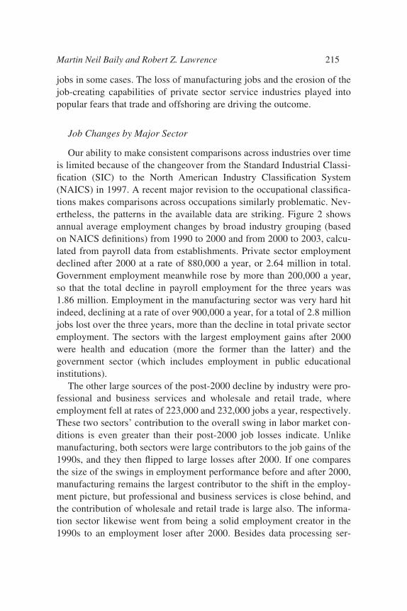
THE BUSINESS CYCLE recovery of the past few years has been an unusualone. In particular, payroll employment since the trough of the 2001 reces-sion has been remarkably weak compared with previous recessions—apoint illustrated in figure 1.2 The decline in payroll employment from thepeak in March 2001 to the trough in November of the same year was mod-est, but employment continued to fall for the next twenty-one months,ending up just over a million jobs below the trough before starting to

211

M A R T I N N E I L B A I L YInstitute for International Economics and McKinsey Global Institute

R O B E R T Z . L A W R E N C EHarvard University and Institute for International Economics

We are grateful to the participants at the Brookings Panel meeting and to Mac Destler,Jeffrey Frankel, Catherine Mann, and Edwin Truman for helpful comments. Thanks alsoto Sunil Patel of NASSCOM for comments. Jacob Kirkegaard, Katharina Plück, andMagali Junowicz provided substantial assistance in the preparation of this paper. VivekAgrawal of McKinsey and Company provided additional assistance with respect to theMcKinsey case study on Indian offshoring. We have benefited greatly from the assistanceof Macroeconomic Advisers in preparing our simulations of the future impact of off-shoring, but the simulations reported using their model should not be taken as predictionsby that organization.

1. Lou Dobbs, “A Home Advantage for U.S. Corporations,” CNN Friday, August 27,2004.

2. This now-familiar figure originated at the Council of Economic Advisers in the1980s, where it was given considerable play “for obvious reasons,” as Michael Mussa hasremarked—job growth after the early 1980s recession was very strong indeed.

2581-03_Lawrence_rev.qxd 1/18/05 13:27 Page 211

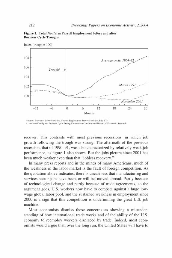
recover. This contrasts with most previous recessions, in which jobgrowth following the trough was strong. The aftermath of the previousrecession, that of 1990–91, was also characterized by relatively weak jobperformance, as figure 1 also shows. But the jobs picture since 2001 hasbeen much weaker even than that “jobless recovery.”

In many press reports and in the minds of many Americans, much ofthe weakness in the labor market is the fault of foreign competition. Asthe quotation above indicates, there is uneasiness that manufacturing andservices sector jobs have been, or will be, moved abroad. Partly becauseof technological change and partly because of trade agreements, so theargument goes, U.S. workers now have to compete against a huge low-wage global labor pool, and the sustained weakness in employment since2000 is a sign that this competition is undermining the great U.S. jobmachine.

Most economists dismiss these concerns as showing a misunder-standing of how international trade works and of the ability of the U.S.economy to reemploy workers displaced by trade. Indeed, most econ-omists would argue that, over the long run, the United States will have to

212 Brookings Papers on Economic Activity, 2:2004

Figure 1. Total Nonfarm Payroll Employment before and after Business Cycle Troughs

100

102

104

106

108

–12 –6 0 6 12 18 24 30

Months

March 1991

November 2001

Average cycle, 1954–82

Source: Bureau of Labor Statistics, Current Employment Survey Statistics, July 2004.a. As identified by the Business Cycle Dating Committee of the National Bureau of Economic Research.

Index (trough = 100)

Trougha

2581-03_Lawrence_rev.qxd 1/18/05 13:27 12

reduce its trade deficit, and that this could create more opportunities forblue-collar workers in export industries. Similarly, the more services theUnited States imports, the larger U.S. exports of both goods and other ser-vices will eventually have to be to pay for them. But economists’ reassur-ances on this point have not carried a lot of weight in the populardebate—or even at times in the policy debate.

Putting the role of trade in the U.S. economy in perspective is not sim-ply a matter of setting the record straight. Misperceptions on the part ofworkers may discourage them from acquiring the skills they need in orderto get good jobs. Misperceptions on the part of voters and elected officialscan lead to bad policies. In this paper, therefore, we try to put trade andelectronic offshoring concerns in the right perspective, in a way that iseasily understandable. We estimate the size of the first-round job disloca-tion that trade and electronic offshoring may have caused between 2000and 2003.3 The approach we use, and several assumptions we make alongthe way, have the effect of exaggerating the impact on trade and off-shoring on the U.S. labor market. Nevertheless, the results show that theweakness in U.S. payroll employment since 2000 has not been caused bya flood of imports of either goods or services. It should certainly not beattributed to any trade agreements the United States has signed.4 Rather,the weakness of employment is primarily the result of inadequate growthof domestic demand in the presence of strong productivity growth.

The paper also goes beyond this basic result in several ways and makesthe following additional findings: First, to the extent that trade did cause aloss of manufacturing jobs, it was the weakness of U.S. exports after 2000and not the strength of imports that was responsible—the share of importsin the U.S. market actually declined. Second, the weakness in U.S.exports was primarily the result of a strong dollar. The world market formanufactured exports continued to grow after 2000, but the United States

Martin Neil Baily and Robert Z. Lawrence 213

3. The use of the terms “offshoring” and “outsourcing” to refer to a wide variety of(often overlapping) activities has created considerable confusion. In this paper we use the term “electronic offshoring” to refer to imports of electronically transmitted services.For a discussion of these terms and one set of definitions, see Bhagwati, Panagariya, and Srinivasan (forthcoming).

4. The North American Free Trade Agreement (NAFTA), in particular, has borne thebrunt of allegations that trade agreements are responsible for large job losses. Yet NAFTAcame into effect in 1995, and the subsequent five years saw very robust employmentgrowth. Hence whatever NAFTA’s employment effects may have been, it is simply im-plausible to blame it for unemployment in 2001 and beyond.


lost market share. Third, the impact on U.S. employment of services sec-tor offshoring to India in 2000–03 was very small compared with theaggregate changes in services sector employment during that period.Fourth, focusing more narrowly on the U.S. technology sector, there hasbeen a loss of lower-paid programming jobs, much of which can be attrib-uted to offshoring to India. But the employment picture for computer ser-vices occupations as a whole has actually been surprisingly strong in thelast few years, especially if one allows for the unsustainable, domesticdemand-driven surge in employment in 2000. Fifth, trade is also unlikelyto be a major source of additional manufacturing jobs in the future: evenif the United States eliminates its merchandise trade deficit over the nextdecade, the net addition to manufacturing employment is likely to bemodest. Sixth and finally, although some have predicted that over 3 mil-lion U.S. service jobs will be offshored via information technologythrough 2015, and simulations from a macroeconomic model suggest thatoffshoring of this magnitude will be large enough to have appreciableeffects on the macroeconomy, the nature of those effects depends cru-cially on how that offshoring is modeled. If offshoring is modeled as adecline in the price at which the United States can buy foreign services,then U.S. GDP, real compensation of employees, and real profits will allbe higher in 2015 as a result of services offshoring. If instead offshoringis modeled simply as an increase in the quantity of services imports attoday’s prices, the welfare benefits will be smaller because more exportsare needed to pay for these. Nonetheless, again, a relatively modest num-ber of jobs are generated in manufacturing to produce these exports. Alltold, our analysis suggests that trade is neither the major source of the cur-rent troubles facing U.S. manufacturing workers nor a potential solutionto their problems in the future.

The Pattern of Employment Change

This section uses detailed data broken down by industry and occupa-tion to review which sectors of the economy have lost jobs in recent yearsand which types of workers lost them. We find that the job losses wereoverwhelmingly concentrated in the manufacturing sector, and that majorservices industries that had been consistent job creators over the 1990sstopped creating jobs after 2000, and indeed lost significant numbers of



jobs in some cases. The loss of manufacturing jobs and the erosion of thejob-creating capabilities of private sector service industries played intopopular fears that trade and offshoring are driving the outcome.

Job Changes by Major Sector

Our ability to make consistent comparisons across industries over timeis limited because of the changeover from the Standard Industrial Classi-fication (SIC) to the North American Industry Classification System(NAICS) in 1997. A recent major revision to the occupational classifica-tions makes comparisons across occupations similarly problematic. Nev-ertheless, the patterns in the available data are striking. Figure 2 showsannual average employment changes by broad industry grouping (basedon NAICS definitions) from 1990 to 2000 and from 2000 to 2003, calcu-lated from payroll data from establishments. Private sector employmentdeclined after 2000 at a rate of 880,000 a year, or 2.64 million in total.Government employment meanwhile rose by more than 200,000 a year,so that the total decline in payroll employment for the three years was1.86 million. Employment in the manufacturing sector was very hard hitindeed, declining at a rate of over 900,000 a year, for a total of 2.8 millionjobs lost over the three years, more than the decline in total private sectoremployment. The sectors with the largest employment gains after 2000were health and education (more the former than the latter) and the government sector (which includes employment in public educationalinstitutions).

The other large sources of the post-2000 decline by industry were pro-fessional and business services and wholesale and retail trade, whereemployment fell at rates of 223,000 and 232,000 jobs a year, respectively.These two sectors’ contribution to the overall swing in labor market con-ditions is even greater than their post-2000 job losses indicate. Unlikemanufacturing, both sectors were large contributors to the job gains of the1990s, and they then flipped to large losses after 2000. If one comparesthe size of the swings in employment performance before and after 2000,manufacturing remains the largest contributor to the shift in the employ-ment picture, but professional and business services is close behind, andthe contribution of wholesale and retail trade is large also. The informa-tion sector likewise went from being a solid employment creator in the1990s to an employment loser after 2000. Besides data processing ser-



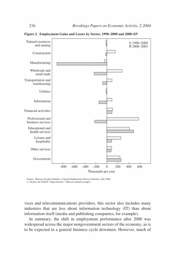
vices and telecommunications providers, this sector also includes manyindustries that are less about information technology (IT) than aboutinformation itself (media and publishing companies, for example).

In summary, the shift in employment performance after 2000 waswidespread across the major nongovernment sectors of the economy, as isto be expected in a general business cycle downturn. However, much of


Figure 2. Employment Gains and Losses by Sector, 1990–2000 and 2000–03a

–800 –600 –400 –200 0 200 400 600

Natural resourcesand mining

Construction

Manufacturing

Wholesale andretail trade

Transportation andwarehousing

Utilities

Information

Financial activities

Professional andbusiness services

Educational andhealth services

Leisure andhospitality

Other services

Government

Thousands per year

1990–20002000–2003

Source: Bureau of Labor Statistics, Current Employment Survey Statistics, July 2004.a. Sectors are NAICS “Super Sectors.” Data are annual averages.


the action was in the three large sectors of manufacturing, professionaland business services, and wholesale and retail trade. Manufacturing isnotable for the very large job losses it suffered, and the other two arenotable because they went from being big job gainers to job losers.5

Job Changes by Occupation

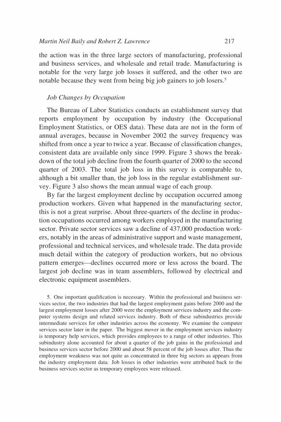
The Bureau of Labor Statistics conducts an establishment survey thatreports employment by occupation by industry (the OccupationalEmployment Statistics, or OES data). These data are not in the form ofannual averages, because in November 2002 the survey frequency wasshifted from once a year to twice a year. Because of classification changes,consistent data are available only since 1999. Figure 3 shows the break-down of the total job decline from the fourth quarter of 2000 to the secondquarter of 2003. The total job loss in this survey is comparable to,although a bit smaller than, the job loss in the regular establishment sur-vey. Figure 3 also shows the mean annual wage of each group.

By far the largest employment decline by occupation occurred amongproduction workers. Given what happened in the manufacturing sector,this is not a great surprise. About three-quarters of the decline in produc-tion occupations occurred among workers employed in the manufacturingsector. Private sector services saw a decline of 437,000 production work-ers, notably in the areas of administrative support and waste management,professional and technical services, and wholesale trade. The data providemuch detail within the category of production workers, but no obviouspattern emerges—declines occurred more or less across the board. Thelargest job decline was in team assemblers, followed by electrical andelectronic equipment assemblers.


5. One important qualification is necessary. Within the professional and business ser-vices sector, the two industries that had the largest employment gains before 2000 and thelargest employment losses after 2000 were the employment services industry and the com-puter systems design and related services industry. Both of these subindustries provideintermediate services for other industries across the economy. We examine the computerservices sector later in the paper. The biggest mover in the employment services industryis temporary help services, which provides employees to a range of other industries. Thissubindustry alone accounted for about a quarter of the job gains in the professional andbusiness services sector before 2000 and about 58 percent of the job losses after. Thus theemployment weakness was not quite as concentrated in three big sectors as appears fromthe industry employment data. Job losses in other industries were attributed back to thebusiness services sector as temporary employees were released.


Fig

ure

3.C

hang

es in

Em

ploy

men

t by

Occ

upat

ion,

200

0–03

–2,0

00–1

,500

–1,0

00–5

0050

00

Food

pre

para

tion

and

serv

ing,

$17

,290

Farm

ing,

fis

hing

, for

estr

y, $

20,2

00B

uild

ing

and

grou

nds

clea

ning

and

mai

nten

ance

, $21

,060

Pers

onal

car

e an

d se

rvic

e, $

21,3

80H

ealth

care

sup

port

, $22

,750

Tra

nspo

rtat

ion

and

mat

eria

l mov

ing,

$27

,600

Off

ice

and

adm

inis

trat

ive

supp

ort,

$28,

260

Prod

uctio

n, $

28,7

10Sa

les

and

rela

ted,

$31

,250

Prot

ectiv

e se

rvic

e, $

34,0

90C

omm

unity

and

soc

ial s

ervi

ces,

$35

,420

Inst

alla

tion,

mai

nten

ance

, rep

air,

$36

,210

Con

stru

ctio

n an

d ex

trac

tion,

$36

,650

Edu

catio

n, tr

aini

ng, a

nd li

brar

y, $

40,6

60A

rt, d

esig

n, e

nter

tain

men

t, sp

orts

and

med

ia, $

42,6

20L

ife,

phy

sica

l and

soc

ial s

cien

ces,

$53

,210

Hea

lthca

re p

ract

ione

rs a

nd te

chni

cal,

$55,

380

Bus

ines

s an

d fi

nanc

ial,

$55,

550

Arc

hite

ctur

e an

d en

gine

erin

g, $

59,2

30C

ompu

ter

and

mat

hem

atic

al, $

63,2

40L

egal

, $78

,910

Man

agem

ent,

mea

n an

nual

wag

e =

$82

,790

Tho

usan

ds o

f w

orke

rs

Sour

ce:

Bur

eau

of L

abor

Sta

tistic

s, O

ccup

atio

nal E

mpl

oym

ent S

tatis

tics

(OE

S).

1,91

1,63

0

1,12

9,20

0


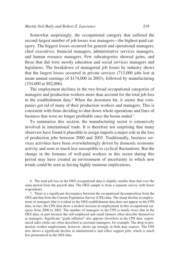
Somewhat surprisingly, the occupational category that suffered thesecond-largest number of job losses was managers—the highest-paid cat-egory. The biggest losses occurred for general and operational managers,chief executives, financial managers, administrative services managers,and human resource managers. Few subcategories showed gains, andthose that did were mostly education and social services managers andlegislators. The breakdown of managerial job losses by industry showsthat the largest losses occurred in private services (713,000 jobs lost atmean annual earnings of $174,000 in 2003), followed by manufacturing(334,000 at $92,000).

The employment declines in the two broad occupational categories ofmanagers and production workers more than account for the total job lossin the establishment data.6 When the downturn hit, it seems that com-panies got rid of many of their production workers and managers. This isconsistent with firms deciding to shut down whole operations and lines ofbusiness that were no longer profitable once the boom ended.7

To summarize this section, the manufacturing sector is extensivelyinvolved in international trade. It is therefore not surprising that manyobservers have found it plausible to assign imports a major role in the lossof production jobs between 2000 and 2003. Traditionally, business ser-vices activities have been overwhelmingly driven by domestic economicactivity and seen as much less susceptible to cyclical fluctuations. But thechange in the fortunes of well-paid workers in this sector during thisperiod may have created an environment of uncertainty in which newtrends could be seen as having highly ominous implications.


6. The total job loss in the OES occupational data is slightly smaller than that over thesame period from the payroll data. The OES sample is from a separate survey with fewerrespondents.

7. There is a significant discrepancy between the occupational decomposition from theOES and that from the Current Population Survey (CPS) data. The sharp decline in employ-ment of managers that is evident in the OES establishment data does not appear in the CPSdata; in fact, the CPS data show a modest increase in employment in this occupational cat-egory from 2000 to 2003. The number of managers in the CPS is nearly twice that in theOES data, in part because the self-employed and small farmers often describe themselvesas managers. Significant “grade inflation” also appears elsewhere in the CPS data: experi-enced sales clerks are often described as assistant managers, for example. The drop in pro-duction worker employment, however, shows up strongly in both data sources. The CPSalso shows a significant decline in administrative and office support jobs, which is muchless pronounced in the OES data.


8. Liz Austin (Associated Press), “Commerce Secretary Announces New Position ofAssistant Secretary for Manufacturing,” Detroit News, September 3, 2003.


The Impact of Trade on the Manufacturing Sector

The recession has bludgeoned the nation’s factories in the past three years, witha record 36 consecutive months of job losses totaling 2.7 million. Low demandat home and abroad, coupled with a flood of imports, have slowed production.8

In this section we use input-output tables of the U.S. economy to esti-mate the direct impact of trade on employment in U.S. manufacturingbetween 2000 and 2003. First, however, we place the recent employmentperformance in historical perspective, explain why the manufacturingtrade deficit has been viewed as an important causal factor in the employ-ment decline, and use GDP data to show that the performance of exports—not imports—is the more important part of the recent employment story.

The manufacturing share of U.S. employment has been declining for atleast half a century. This is not unique to the United States, however; it istypical of developed economies and even characteristic of many develop-ing economies. The basic reason is that although demand for the output ofthe manufacturing sector has grown about as rapidly as GDP, it has not

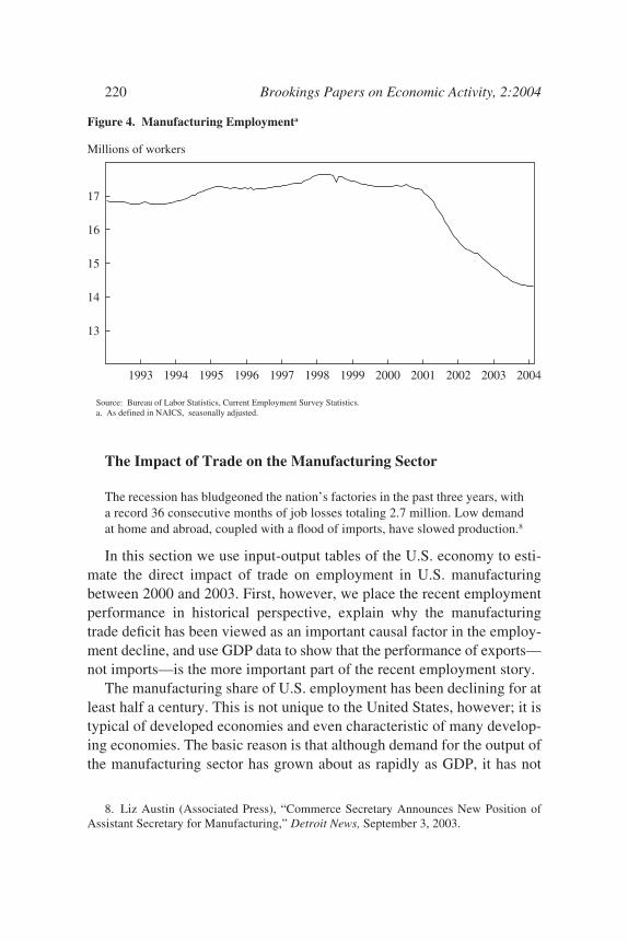
Figure 4. Manufacturing Employmenta

13

14

15

16

17

1993 1994 1995 1996 1997 1998 1999 2000 2001 2002 2003 2004

Source: Bureau of Labor Statistics, Current Employment Survey Statistics.a. As defined in NAICS, seasonally adjusted.

Millions of workers



grown fast enough to offset the relatively rapid productivity growth in thesector.9 As a result, the relative demand for manufacturing workers hasdeclined.10

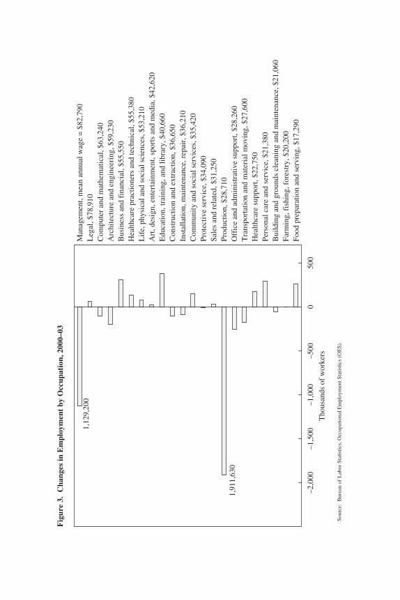
Some observers explain the recent job loss in manufacturing by point-ing to the relatively rapid manufacturing productivity growth of recentyears, but between 2000 and 2003 this factor did not play a dominant role.Over that period the share of manufacturing in nonfarm payrolls fell from13.1 percent to 11.1 percent—a drop of 15 percent. But the 12 percent in-crease in nonfarm output per worker-hour between 2000 and 2003 wasonly 3 percentage points less than the increase in manufacturing laborproductivity. This leaves 80 percent (12 percentage points of the 15 percent)of the decline in manufacturing’s employment share to be explained byother factors.11

Moreover, the concerns were more about absolute job loss than aboutmanufacturing’s declining share. As figure 4 illustrates, in the decade ofthe 1990s, the absolute level of employment in manufacturing remainedfairly stable. In fact, between 1993 and 1998 manufacturing payrollsincreased from 16.8 million to 17.6 million, almost regaining their 1989peak of 18 million. They then declined modestly to 17.3 million by 2000.Thereafter, however, manufacturing employment fell precipitously.Between 2000 and 2003 payroll employment in manufacturing fell 16.2 percent—the largest slump in manufacturing employment in postwarhistory.12

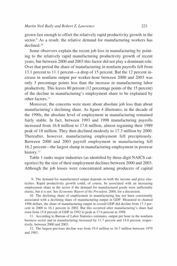
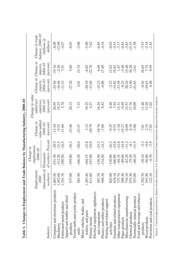
Table 1 ranks major industries (as identified by three-digit NAICS cat-egories) by the size of their employment declines between 2000 and 2003.Although the job losses were concentrated among producers of capital

9. The demand for manufactured output depends on both the income and price elas-ticities. Rapid productivity growth could, of course, be associated with an increasingemployment share in the sector if the demand for manufactured goods were sufficientlyelastic, but it is not. See Economic Report of the President, 2004, for a discussion.

10. The declining share of employment in manufacturing has not been consistentlyassociated with a declining share of manufacturing output in GDP. Measured in chained1996 dollars, the share of manufacturing output in overall GDP did decline from 17.3 per-cent in 2000 to 16.1 percent in 2002. But this occurred after manufacturing’s share hadrisen from 15.8 percent of GDP in 1992 to peak at 17.6 percent in 1998.

11. According to Bureau of Labor Statistics estimates, output per hour in the nonfarmbusiness sector and in manufacturing increased by 11.7 percent and 14.8 percent, respec-tively, between 2000 and 2003.

12. The largest previous decline was from 19.4 million to 16.7 million between 1979and 1983.


Tab

le 1

.C

hang

es in

Em

ploy

men

t an

d T

rade

Bal

ance

by

Man

ufac

turi

ng I

ndus

try,

200

0–03

Cha

nge

in v

alue

Em

ploy

men

t,C

hang

e in

adde

d pe

rC

hang

e in

Cha

nge

inC

hang

e in

trad

e20

00va

lue

adde

d,em

ploy

ee,

expo

rts,

impo

rts,

bala

nce,

200

0–03

(tho

usan

ds o

fT

hous

ands

2000

–03

2000

–03

2000

–03

2000

–03

(bil

lion

s of

Indu

stry

wor

kers

)of

wor

kers

Per

cent

(per

cent

)(p

erce

nt)

(per

cent

)(p

erce

nt)

doll

ars)

Com

pute

r an

d el

ectr

onic

pro

duct

s1,

863.

50–5

31.3

0–2

8.5

–13.

5420

.95

–23.

56–1

5.16

–8.0

9M

achi

nery

1,45

2.60

–312

.20

–21.

5–9

.53

15.2

3–1

6.46

–2.2

6–1

2.98

Fabr

icat

ed m

etal

pro

duct

s1,

761.

70–2

90.5

0–1

6.5

–11.

665.

78–1

1.12

7.51

–4.6

7A

ppar

el a

nd le

athe

r an

d al

lied

prod

ucts

537.

00–1

95.0

0–3

6.3

–23.

4820

.15

–27.

205.

88–8

.03

Tex

tile

mill

s an

d te

xtile

pro

duct

m

ills

581.

50–1

66.2

0–2

8.6

–23.

477.

152.

0115

.74

–2.0

8M

otor

veh

icle

s, b

odie

s, a

nd

trai

lers

, and

par

ts1,

283.

46–1

64.1

5–1

2.8

3.12

18.2

5–2

0.10

–6.8

2–5

.80

Prim

ary

met

als

611.

60–1

47.0

0–2

4.0

–20.

794.

27–1

1.04

–22.

787.

62E

lect

rica

l equ

ipm

ent,

appl

ianc

es,

and

com

pone

nts

587.

70–1

36.5

0–2

3.2

–10.

7616

.24

–15.

236.

68–6

.85

Plas

tics

and

rubb

er p

rodu

cts

940.

30–1

34.5

0–1

4.3

–7.0

98.

42–6

.80

17.8

9–4

.34

Prin

ting

and

rela

ted

supp

ort

activ

ities

801.

00–1

30.9

0–1

6.3

–9.2

58.

48–2

.23

12.0

2–0

.62

Furn

iture

and

rel

ated

pro

duct

s67

6.10

–106

.80

–15.

8–9

.53

7.44

–15.

8225

.82

–4.5

1O

ther

tran

spor

tatio

n eq

uipm

ent

737.

74–9

4.35

–12.

8–1

.18

13.3

1–1

3.39

1.47

–7.1

7Pa

per

prod

ucts

599.

30–8

9.00

–14.

9–1

5.27

–0.4

9–9

.23

–3.4

8–0

.81

Mis

cella

neou

s m

anuf

actu

ring

734.

10–8

2.20

–11.

2–0

.09

12.5

120

.24

15.4

8–3

.83

Che

mic

al p

rodu

cts

975.

20–7

9.30

–8.1

8.18

17.7

613

.40

36.2

8–1

5.33

Non

met

allic

min

eral

pro

duct

s55

3.60

–66.

10–1

1.9

–3.0

610

.09

–21.

63–2

.61

–1.3

8Fo

od a

nd b

ever

age

and

toba

cco

pr

oduc

ts1,

762.

70–5

8.10

–3.3

7.81

11.4

8–0

.42

26.6

5–7

.53

Woo

d pr

oduc

ts59

3.50

–56.

90–9

.62.

3513

.20

–19.

637.

74–2

.18

Petr

oleu

m a

nd c

oal p

rodu

cts

122.

10–9

.70

–7.9

–7.0

11.

026.

989.

59–1

.81

Sou

rces

:C

urre

nt E

mpl

oym

ent S

urve

y, B

urea

u of

Lab

or S

tati

stic

s; U

.S. I

nter

nati

onal

Tra

de C

omm

issi

on; B

urea

u of

Eco

nom

ic A

naly

sis.

Cha

nge

inem

ploy

men

t,20

00–0

3


goods and apparel, every three-digit industry saw its payrolls fall. Thebursting of the high-technology bubble resulted in the loss of more thanhalf a million jobs in the industry that produces computers and electronicproducts—fully 28.5 percent of the industry’s 2000 employment. Otherlarge declines occurred in machinery (312,000 jobs lost, or 21.5 percent)and fabricated metal products (290,000, or 16.5 percent). Apparel andleather (195,000 jobs lost, or 36.3 percent) and textile product mills(166,200, or 28.6 percent) were severely affected. Table 1 also shows thechange in value added by industry and in value added per employee—important drivers of employment change whose role will be featured inthe later analysis.

To many observers, trade was the obvious culprit for these job losses.The United States has run increasing deficits in manufacturing trade since1992. These deficits have been both large relative to the size of the sectorand growing. The growth in the deficit has been particularly pronouncedsince 1997, when U.S. exports stagnated in the aftermath of the Asianfinancial crisis while U.S. imports increased rapidly as the economyboomed. As a result, between 1997 and 2000 the trade deficit in manufac-tured goods more than doubled, from $136 billion to $317 billion. Astable 2 indicates, between 2000 and 2003 the trade balance in manufac-turing declined by an additional $86.1 billion, predominantly becauseexports fell by $62.3 billion (8.8 percent), although imports also in-creased, by $23.6 billion (2.3 percent).

Table 1 illustrates that declining trade balances were widespreadacross industries between 2000 and 2003. Only one of the nineteen in-dustries in manufacturing—primary metals—avoided a decline in itstrade balance over the period. The sectors with the largest declines werechemical products ($15.3 billion), machinery ($13.0 billion), computers ($8.1 billion), apparel ($8.0 billion), and food ($7.5 billion). Export per-formance was particularly weak: exports fell in fifteen of the nineteenindustries. The largest percentage declines were in apparel (down $3 bil-lion, or 27.2 percent), computers ($46 billion, or 23.6 percent), and motorvehicles ($8 billion, or 20.1 percent). Other large declines were in ma-chinery (down $15 billion) and other transportation (which includes air-craft; down $6.5 billion).

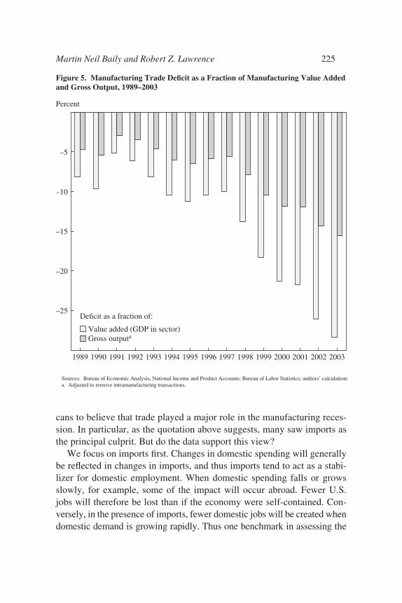
How do these deficits compare with overall manufacturing output?Figure 5 shows the manufacturing trade deficit as a percentage of manu-facturing output, with output measured in two different ways. The first



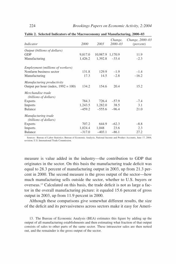
measure is value added in the industry—the contribution to GDP thatoriginates in the sector. On this basis the manufacturing trade deficit wasequal to 28.3 percent of manufacturing output in 2003, up from 21.3 per-cent in 2000. The second measure is the gross output of the sector—howmuch manufacturing sells outside the sector, whether to U.S. buyers oroverseas.13 Calculated on this basis, the trade deficit is not as large a fac-tor in the overall manufacturing picture: it equaled 15.6 percent of grossoutput in 2003, up from 11.9 percent in 2000.

Although these comparisons give somewhat different results, the sizeof the deficit and its pervasiveness across sectors make it easy for Ameri-


13. The Bureau of Economic Analysis (BEA) estimates this figure by adding up theoutput of all manufacturing establishments and then estimating what fraction of that outputconsists of sales to other parts of the same sector. These intrasector sales are then nettedout, and the remainder is the gross output of the sector.

Table 2. Selected Indicators of the Macroeconomy and Manufacturing, 2000–03

Change, Change, 2000–03Indicator 2000 2003 2000–03 (percent)

Output (billions of dollars)GDP 9,817.0 10,987.9 1,170.9 11.9Manufacturing 1,426.2 1,392.8 –33.4 –2.3

Employment (millions of workers)Nonfarm business sector 131.8 129.9 –1.9 –1.4Manufacturing 17.3 14.5 –2.8 –16.2

Manufacturing productivityOutput per hour (index, 1992 = 100) 134.2 154.6 20.4 15.2

Merchandise trade (billions of dollars)

Exports 784.3 726.4 –57.9 –7.4Imports 1,243.5 1,282.0 38.5 3.1Balance –459.2 –555.6 –96.4 21.0

Manufacturing trade (billions of dollars)

Exports 707.2 644.9 –62.3 –8.8Imports 1,024.4 1,048 23.6 2.3Balance –317.0 –403.1 –86.1 27.2

Sources: Bureau of Labor Statistics; Bureau of Economic Analysis, National Income and Product Accounts, June 17, 2004,revision; U.S. International Trade Commission.


cans to believe that trade played a major role in the manufacturing reces-sion. In particular, as the quotation above suggests, many saw imports asthe principal culprit. But do the data support this view?

We focus on imports first. Changes in domestic spending will generallybe reflected in changes in imports, and thus imports tend to act as a stabi-lizer for domestic employment. When domestic spending falls or growsslowly, for example, some of the impact will occur abroad. Fewer U.S.jobs will therefore be lost than if the economy were self-contained. Con-versely, in the presence of imports, fewer domestic jobs will be created whendomestic demand is growing rapidly. Thus one benchmark in assessing the


Figure 5. Manufacturing Trade Deficit as a Fraction of Manufacturing Value Addedand Gross Output, 1989–2003

–25

–20

–15

–10

–5

1989 1990 1991 1992 1993 1994 1995 1996 1997 1998 1999 2000 2001 2002 2003

Percent

Value added (GDP in sector)Gross outputa

Sources: Bureau of Economic Analysis, National Income and Product Accounts; Bureau of Labor Statistics; authors’ calculationsa. Adjusted to remove intramanufacturing transactions.

Deficit as a fraction of:


impact of imports is whether or not they are rising faster than domesticspending. In general, if imports were a major independent cause of jobloss, one might expect to see them outpacing domestic spending; if theywere simply responding to shifts in domestic spending, they would rise atthe same pace; and if they were acting to stabilize employment wherespending was weak, they would rise more slowly than spending.

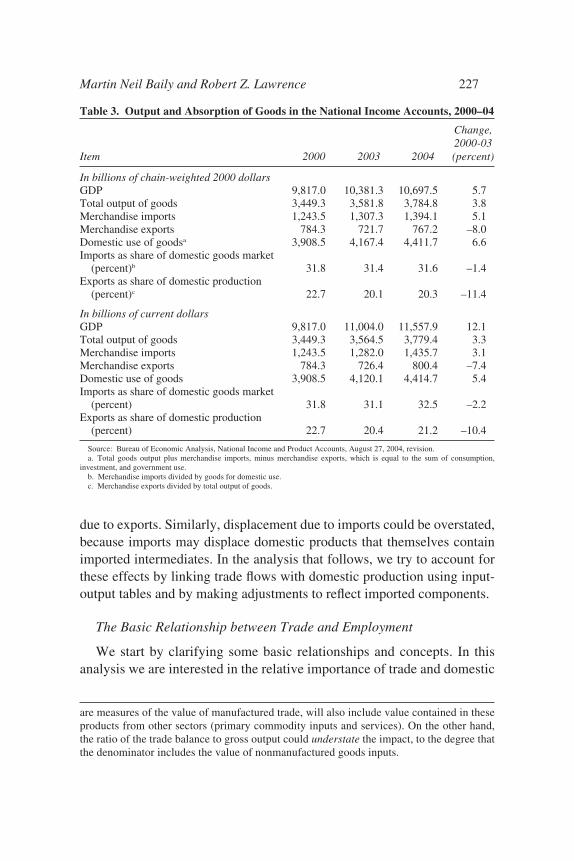
Table 3 provides some perspective on the role of goods in U.S. GDP. Itis important to note that these data measure final sales of goods. In addi-tion to manufacturing value added, therefore, they include distributionmargins and primary commodity inputs, issues we will deal with later.Nonetheless, they provide important insights into this question. Between2000 and 2003, measured in 2000 chain-weighted dollars, the volume ofmerchandise imports grew by 5.1 percent, a pace that was actually slowerthan U.S. domestic spending on goods for domestic use (consumption,investment, and government spending), which increased by 6.6 percent.In 2000 dollars, therefore, the share of imports in U.S. domestic spendingon goods actually fell from 31.8 percent to 31.4 percent. (In current dol-lars there was a slightly larger decline in the import share.)

The export story is different. Here one benchmark is the share ofexports in domestic goods output. Between 2000 and 2003, goods outputincreased by 3.8 percent, but the volume of merchandise exports actuallydeclined by 8.0 percent. This led to a decline in the share of goods exportsin goods output from 23 percent to 20 percent. Together with the importdata, these data suggest that falling exports detracted from employment,and not that a rising share of imports led to disproportionate unemployment.

Although highly suggestive, measures such as these may fail to accu-rately indicate the size of the trade effects on the manufacturing sector,because they include value added in other sectors.14 Trade flows operate onthe demand for labor in manufacturing in complex ways. First, manufac-tured exports are not produced entirely within the manufacturing sector:manufactured goods also embody value added from other sectors, such asservices and primary commodities. Second, and conversely, trade in non-manufactured goods and services will embody manufactured goods. Andthird, many goods produced in the United States contain imported compo-nents. Ignoring this could lead to an overstatement of U.S. employment


14. On the one hand, the ratio of the trade balance to value added will overstate thecontribution of trade to manufacturing, because the components in the numerator, which


due to exports. Similarly, displacement due to imports could be overstated,because imports may displace domestic products that themselves containimported intermediates. In the analysis that follows, we try to account forthese effects by linking trade flows with domestic production using input-output tables and by making adjustments to reflect imported components.

The Basic Relationship between Trade and Employment

We start by clarifying some basic relationships and concepts. In thisanalysis we are interested in the relative importance of trade and domestic


are measures of the value of manufactured trade, will also include value contained in theseproducts from other sectors (primary commodity inputs and services). On the other hand,the ratio of the trade balance to gross output could understate the impact, to the degree thatthe denominator includes the value of nonmanufactured goods inputs.

Table 3. Output and Absorption of Goods in the National Income Accounts, 2000–04

Change,2000-03

Item 2000 2003 2004 (percent)

In billions of chain-weighted 2000 dollarsGDP 9,817.0 10,381.3 10,697.5 5.7Total output of goods 3,449.3 3,581.8 3,784.8 3.8Merchandise imports 1,243.5 1,307.3 1,394.1 5.1Merchandise exports 784.3 721.7 767.2 –8.0Domestic use of goodsa 3,908.5 4,167.4 4,411.7 6.6Imports as share of domestic goods market

(percent)b 31.8 31.4 31.6 –1.4Exports as share of domestic production

(percent)c 22.7 20.1 20.3 –11.4

In billions of current dollarsGDP 9,817.0 11,004.0 11,557.9 12.1Total output of goods 3,449.3 3,564.5 3,779.4 3.3Merchandise imports 1,243.5 1,282.0 1,435.7 3.1Merchandise exports 784.3 726.4 800.4 –7.4Domestic use of goods 3,908.5 4,120.1 4,414.7 5.4Imports as share of domestic goods market

(percent) 31.8 31.1 32.5 –2.2Exports as share of domestic production

(percent) 22.7 20.4 21.2 –10.4

Source: Bureau of Economic Analysis, National Income and Product Accounts, August 27, 2004, revision.a. Total goods output plus merchandise imports, minus merchandise exports, which is equal to the sum of consumption,

investment, and government use.b. Merchandise imports divided by goods for domestic use.c. Merchandise exports divided by total output of goods.


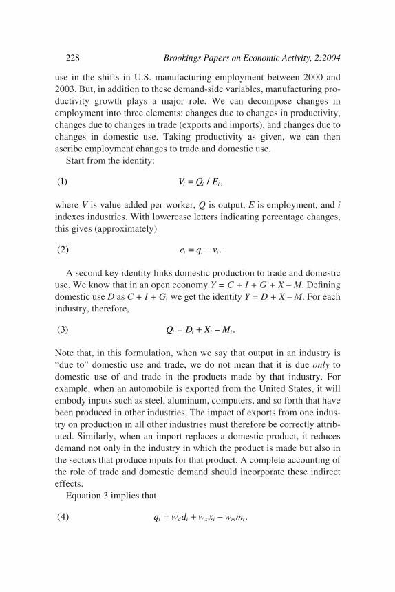
use in the shifts in U.S. manufacturing employment between 2000 and2003. But, in addition to these demand-side variables, manufacturing pro-ductivity growth plays a major role. We can decompose changes inemployment into three elements: changes due to changes in productivity,changes due to changes in trade (exports and imports), and changes due tochanges in domestic use. Taking productivity as given, we can thenascribe employment changes to trade and domestic use.

Start from the identity:

where V is value added per worker, Q is output, E is employment, and iindexes industries. With lowercase letters indicating percentage changes,this gives (approximately)

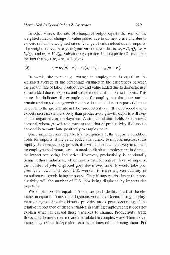
A second key identity links domestic production to trade and domesticuse. We know that in an open economy Y = C + I + G + X – M. Definingdomestic use D as C + I + G, we get the identity Y = D + X – M. For eachindustry, therefore,

Note that, in this formulation, when we say that output in an industry is“due to” domestic use and trade, we do not mean that it is due only todomestic use of and trade in the products made by that industry. Forexample, when an automobile is exported from the United States, it willembody inputs such as steel, aluminum, computers, and so forth that havebeen produced in other industries. The impact of exports from one indus-try on production in all other industries must therefore be correctly attrib-uted. Similarly, when an import replaces a domestic product, it reducesdemand not only in the industry in which the product is made but also inthe sectors that produce inputs for that product. A complete accounting ofthe role of trade and domestic demand should incorporate these indirecteffects.

Equation 3 implies that

( ) – .4 q w d w x w mi d i x i m i= +

( ) – .3 Q D X Mi i i i= +

( ) .2 e q vi i i= −

( ) / ,1 V Q Ei i i=



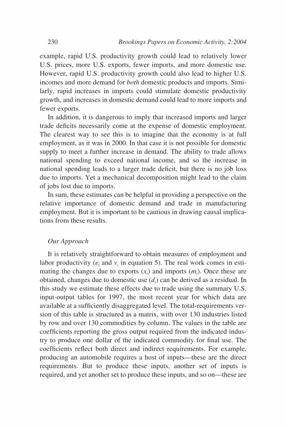
In other words, the rate of change of output equals the sum of theweighted rates of change in value added due to domestic use and due toexports minus the weighted rate of change of value added due to imports.The weights reflect base-year (year zero) shares; that is, wd = D0/Q0 , wx =X0/Q0, and wm = M0/Q0. Substituting equation 4 into equation 2, and usingthe fact that wd + wx – wm = 1, gives

In words, the percentage change in employment is equal to theweighted average of the percentage changes in the differences betweenthe growth rate of labor productivity and value added due to domestic use,value added due to exports, and value added attributable to imports. Thisexpression indicates, for example, that for employment due to exports toremain unchanged, the growth rate in value added due to exports (xi) mustbe equal to the growth rate in labor productivity (vi). If value added due toexports increases more slowly than productivity growth, exports will con-tribute negatively to employment. A similar relation holds for domesticdemand, whose growth rate must exceed that of productivity if domesticdemand is to contribute positively to employment.

Since imports enter negatively into equation 5, the opposite conditionholds for imports. If the value added attributable to imports increases lessrapidly than productivity growth, this will contribute positively to domes-tic employment. Imports are assumed to displace employment in domes-tic import-competing industries. However, productivity is continuallyrising in these industries, which means that, for a given level of imports,the number of jobs displaced goes down over time. It would take pro-gressively fewer and fewer U.S. workers to make a given quantity ofmanufactured goods being imported. Only if imports rise faster than pro-ductivity will the number of U.S. jobs being displaced by imports riseover time.

We emphasize that equation 5 is an ex post identity and that the ele-ments in equation 5 are all endogenous variables. Decomposing employ-ment changes using this identity provides an ex post accounting of therelative importance of these variables in shifting employment; it does notexplain what has caused these variables to change. Productivity, tradeflows, and domestic demand are interrelated in complex ways. Their move-ments may reflect independent causes or interactions among them. For

( ) – – – – .5 e w d v w x v w m vi d i i x i i m i i= ( ) + ( ) ( )



example, rapid U.S. productivity growth could lead to relatively lowerU.S. prices, more U.S. exports, fewer imports, and more domestic use.However, rapid U.S. productivity growth could also lead to higher U.S.incomes and more demand for both domestic products and imports. Simi-larly, rapid increases in imports could stimulate domestic productivitygrowth, and increases in domestic demand could lead to more imports andfewer exports.

In addition, it is dangerous to imply that increased imports and largertrade deficits necessarily come at the expense of domestic employment.The clearest way to see this is to imagine that the economy is at fullemployment, as it was in 2000. In that case it is not possible for domesticsupply to meet a further increase in demand. The ability to trade allowsnational spending to exceed national income, and so the increase innational spending leads to a larger trade deficit, but there is no job lossdue to imports. Yet a mechanical decomposition might lead to the claimof jobs lost due to imports.

In sum, these estimates can be helpful in providing a perspective on therelative importance of domestic demand and trade in manufacturingemployment. But it is important to be cautious in drawing causal implica-tions from these results.

Our Approach

It is relatively straightforward to obtain measures of employment andlabor productivity (ei and vi in equation 5). The real work comes in esti-mating the changes due to exports (xi) and imports (mi). Once these areobtained, changes due to domestic use (di) can be derived as a residual. Inthis study we estimate these effects due to trade using the summary U.S.input-output tables for 1997, the most recent year for which data areavailable at a sufficiently disaggregated level. The total-requirements ver-sion of this table is structured as a matrix, with over 130 industries listedby row and over 130 commodities by column. The values in the table arecoefficients reporting the gross output required from the indicated indus-try to produce one dollar of the indicated commodity for final use. Thecoefficients reflect both direct and indirect requirements. For example,producing an automobile requires a host of inputs—these are the directrequirements. But to produce these inputs, another set of inputs isrequired, and yet another set to produce these inputs, and so on—these are



the indirect requirements. The coefficients in the matrix capture all ofthese effects.

As an example, for each dollar of final delivery of motor vehicles, thelargest total requirement is output of 99.8 cents by the motor vehiclemanufacturing industry. In addition, 53.3 cents of output is requiredfrom the industry titled “motor vehicle body, trailer and parts manufac-turing,” 13.1 cents from wholesale trade, 6.9 cents from electrical equip-ment manufacturing, 5.7 cents from plastics, and so on. All told, 288.8cents are required from the economy as a whole to produce a dollar’sworth of motor vehicles delivered to final demand. (This figure exceedsone dollar because it captures the value of all components along thevalue chain as well as final output.) To obtain our estimates, we gothrough five calculations.

value added. First, since we are interested in estimating value addedby industry, we multiply each of the matrix coefficients by the 1997 ratioof value added to gross output for each industry. This provides us withestimates of the direct and indirect value added required from each indus-try to produce a dollar of final demand. For motor vehicles, for example,the ratio of value added to output was 0.156. Thus the 99.8 cents’ worth offinal demand for motor vehicles was associated with 15.6 cents of valueadded in motor vehicles.15

aggregation. To make our work tractable and intelligible, we thenaggregate these value-added coefficients to provide estimates at the three-digit NAICS level, which, for example, divides manufacturing intonineteen industries. We aggregate the commodities by weighting the co-efficients in the columns comprising parts of the three-digit sector by theshare of each commodity in the total commodity output of that sector.16

We then sum the coefficients in the rows that make up each three-digit


15. Let IO = total requirements table and IOv = total value added requirements table.v = vector of the ratio of value added to gross output by industry (from the 1997

input-output use table) go = vector of gross output (from the 1997 input-output use table):

(1) v = va/go(2) IOv = v * IO

16. If Cij are the coefficients of the matrix IO, we need to obtain new coefficients Cik,for a matrix IO3d with three-digit industry requirements. We first collapse the number ofcolumns using growth outputs in the industry subsectors as weights. We obtain Cik =(ci1*go1 + ci2*go2 + . . . + ciJ*goJ)/(go1 + go2 + . . . + goJ), with j = 1, 2, . . . , J and go1 + go2

+ . . . + goJ = gok. Then we aggregate these Cik for all is in each three-digit industry.


industry. This results in a matrix that estimates direct and indirect valueadded at the three-digit level.

value added due to trade. Under the assumption that the intersec-toral relationships between 2000 and 2003 are the same as those of 1997,we then use three-digit NAICS trade data to estimate the value added ineach three-digit manufacturing industry that is embodied in merchandisetrade in 2000, 2002, and 2003. We obtain separate estimates for exportsand imports.17

correcting for imported components. These value-added compo-nents are upper-bound estimates of the effects due to exports and imports,because the requirements table is derived under the assumption that allinputs are produced domestically. To account for imported componentsused as intermediate inputs, we adjust the requirements by assuming thatimported inputs are purchased in proportion to their share in the domesticmarket, where the domestic market is defined for each industry as the sumof gross output and imports.18 (We will also report our aggregate resultswithout making this correction.)

employment. The final step involves estimating the employmentcontent of value added. We assume that productivity in each U.S. indus-try is the same whether the production is for export, to replace imports,or to serve other domestic demand. This implies that the relative alloca-tions of employment to exports, import substitution, and domestic use,within each industry, are the same as the relative allocations of valueadded.

Data on value added per employee for manufacturing industries areavailable for 2000 and 2002. To correspond to the trade data, which are incurrent dollars, we use current-dollar value added per employee. Neitherreal nor nominal value added per employee is available by industry for2003, and so we estimate the 2003 figure by multiplying the 2002 data bythe growth in the industry-level industrial production index and the indus-try producer price index between 2002 and 2003. Dividing industry valueadded due to exports and imports by value added per worker provides uswith estimates of industry employment “due to” exports and imports.


17. X * IO3d = vaX (total value added of exports)M * IO3d = vaM (total value added of imports).

18. adjvaX = vaX * {1 – [m/(go + m)]} (total value added of exports adjusting byimported inputs) and adjvaM = vaM * [m/(go + m)] (total value added of imports adjustingby imported inputs).


Finally, we estimate employment due to domestic use as a residual—thedifference between actual employment and employment due to trade.

In addition to the caveats given earlier, we note that input-output co-efficients allow for no substitution possibilities among inputs and no changesin input requirements over time. Furthermore, among products, the analy-sis assumes that final demands always substitute between particularimports and the output of the domestic industry that manufactures prod-ucts similar to those imports, rather than between particular imports andproducts of some other industry.

Results

Trade plays an important role in manufacturing employment. In 2000production for export accounted for 3.43 million manufacturing jobs, or20 percent of manufacturing employment. Each dollar of exports wasassociated with 48 cents of manufacturing value added, with the rest com-ing from imported inputs and other domestic sectors. Each million dollarsin exports, therefore, required 5.2 jobs in manufacturing. On average,these jobs were associated with high levels of labor productivity. Outputper employee engaged in export production was $91,700, considerablyhigher than either the $80,700 in manufacturing as a whole or the $84,600for domestic production that replaces imports.

Between 2000 and 2003, productivity growth in manufacturing wasremarkably rapid. Our estimated measure of nominal value added peremployee increased by 15.3 percent over the three years, just about thesame as the official measure of (real) output per worker-hour in manufac-turing estimated by the Bureau of Labor Statistics. We estimate that pro-duction for export accounted for 3.43 million jobs in 2000. In 2000 valueadded per employee in U.S. manufacturing was $80,700. We estimate thatby 2003 this had increased to $93,100. Had demand remained constant,manufacturing employment would have fallen by 2.64 million—onlyslightly less than the actual total loss of 2.74 million jobs between 2000and 2003. Thus one way to interpret the data is to say that the decline isentirely “due to” domestic productivity growth. Taking output as given, inother words, productivity improvements caused all the job loss.

However, an alternative approach is to see how domestic use and tradecontributed to the decline, taking productivity growth as given—an analy-sis we are now in a position to undertake. As equation 5 indicates, given


2581-03_Lawrence_rev.qxd 1/18/05 13:27 3

productivity growth, a sufficient condition for aggregate employment tohave remained constant would have been for value added due to domesticdemand, exports, and imports to rise by 15.3 percent each. Instead valueadded due to domestic demand and imports increased by just 0.3 percentand 2.4 percent, respectively, while value added due to exports actuallyfell by 11.1 percent. The result was the precipitous 15.9 percent slump inemployment.

Our estimates point to the failure of domestic demand growth to matchproductivity growth as the major source of the decline. We attribute 88 percent of the drop, or some 2.5 million jobs, to the slow growth indomestic demand (table 4); we attribute only 12 percent, or some 314,000jobs, to trade. Although the employment decline attributable to exportsplayed a major role, accounting for 28 percent of the drop, or 742,000jobs, imports actually offset this fall by 429,000 jobs and thus had a posi-tive effect as judged by this baseline. This positive effect arises partlybecause of rapid productivity growth and partly because of the slowgrowth of imports, the manufacturing job content of U.S. imports (whichhave a negative impact on employment) was actually 8.8 percent lowerthan in 2000.19

Imports mitigated the job loss in manufacturing over 2000–03, but notbecause of an exogenous downward shock to imports. There is no evi-dence that the United States was suddenly able to compete more effec-tively against foreign producers. The slow growth of imports was due tothe slow growth in overall U.S. demand, which affected both domesticsuppliers of manufactured goods and foreign suppliers.

In the above estimates we have adjusted the input-output coefficientsto take account of imported inputs. This has the effect of reducing the esti-mated impact of trade flows by reducing the domestic value added due toexports and that due to imports. When we do not make these adjustments,therefore, we get somewhat larger effects due to trade and thus smallereffects due to domestic demand, but qualitatively the results are the same.Using this approach, the net impact of trade on manufacturing job lossrises from 314,000 to 341,000.20


19. Between 2000 and 2003, value added per employee due to exports and importsincreased by 13.7 percent and 12.3 percent, respectively, both somewhat less than theincrease in value added in manufacturing as a whole.

20. Without the import correction, between 2000 and 2003, 951,000 jobs are lostbecause of lower exports and 611,000 jobs are gained because of lower imports.


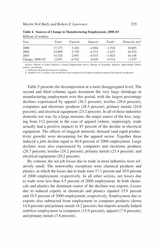
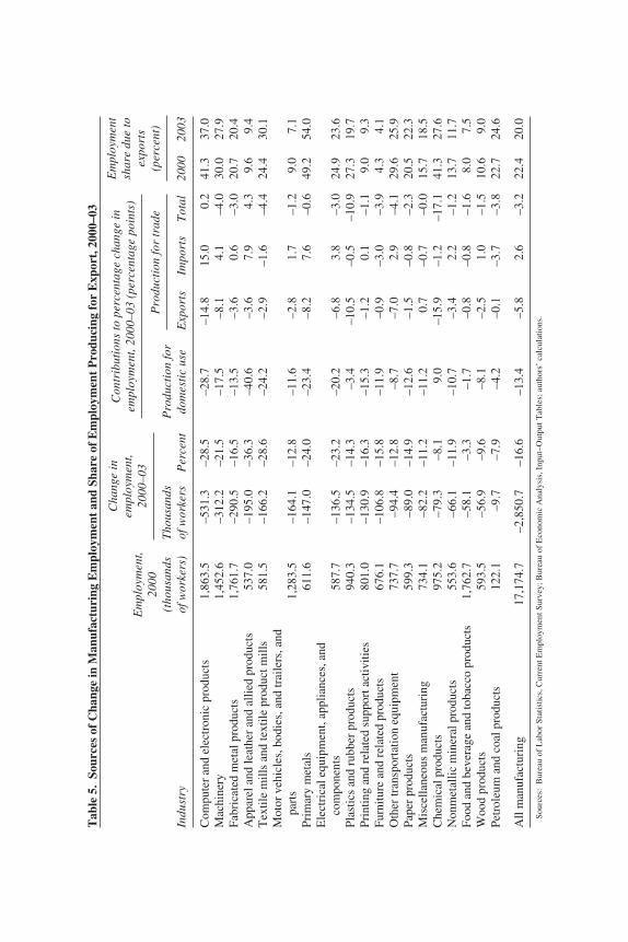
Table 5 presents the decomposition at a more disaggregated level. Thesecond and third columns again document the very large shrinkage inmanufacturing employment over this period, with the largest percentagedeclines experienced by apparel (36.3 percent), textiles (28.6 percent),computers and electronic products (28.5 percent), primary metals (24.0percent), and electrical equipment (23.2 percent). In all of these industriesdomestic use was, by a large measure, the major source of the loss, rang-ing from 112 percent in the case of apparel (where, surprisingly, tradeactually had a positive impact) to 87 percent of the decline in electricalequipment. The effects of sluggish domestic demand (and rapid produc-tivity growth) were devastating for the apparel sector. Together theseinduced a jobs decline equal to 40.6 percent of 2000 employment. Largedeclines were also experienced by computers and electronic products(28.7 percent), textiles (24.2 percent), primary metals (23.4 percent), andelectrical equipment (20.2 percent).

By contrast, the net job losses due to trade in most industries were rel-atively small. The noteworthy exceptions were chemical products andplastics, in which the losses due to trade were 17.1 percent and 10.9 percentof 2000 employment, respectively. In all other sectors, net losses due to trade were less than 4.5 percent of 2000 employment. In both chemi-cals and plastics the dominant source of the declines was exports. Losses due to reduced exports in chemicals and plastics equaled 15.9 percent and 10.5 percent of 2000 employment, respectively. Employment due toexports also subtracted from employment in computer products (down14.8 percent) and primary metals (8.2 percent), but imports actually helpedstabilize employment in computers (15.0 percent), apparel (7.9 percent),and primary metals (7.6 percent).


Table 4. Sources of Change in Manufacturing Employment, 2000–03Millions of workers

Year Total Exports Imports Tradea Domestic useb

2000 17.175 3.434 –4.944 –1.510 18.6852002 14.899 2.739 –4.372 –1.633 16.5322003 14.324 2.691 –4.515 –1.824 16.148Change, 2000–03 –2.851 –0.742 0.429 –0.314 –2.537

Sources: Bureau of Labor Statistics, Current Employment Survey; Bureau of Economic Analysis, Input-Output Tables;authors’ calculations.

a. Difference between previous two columns. b. Number of U.S. workers who would have been employed if all imports had been replaced by domestic production.


Tab

le 5

.So

urce

s of

Cha

nge

in M

anuf

actu

ring

Em

ploy

men

t an

d Sh

are

of E

mpl

oym

ent

Pro

duci

ng f

or E

xpor

t, 2

000–

03

Em

ploy

men

t,20

00(t

hous

ands

Tho

usan

dsP

rodu

ctio

n fo

rIn

dust

ryof

wor

kers

)of

wor

kers

Per

cent

dom

esti

c us

eE

xpor

tsIm

port

sT

otal

2000

2003

Com

pute

r an

d el

ectr

onic

pro

duct

s1,

863.

5–5

31.3

–28.

5–2

8.7

–14.

815

.00.

241

.337

.0M

achi

nery

1,45

2.6

–312

.2–2

1.5

–17.

5–8

.14.

1–4

.030

.027

.9Fa

bric

ated

met

al p

rodu

cts

1,76

1.7

–290

.5–1

6.5

–13.

5–3

.60.

6–3

.020

.720

.4A

ppar

el a

nd le

athe

r an

d al

lied

prod

ucts

537.

0–1

95.0

–36.

3–4

0.6

–3.6

7.9

4.3

9.6

9.4

Tex

tile

mill

s an

d te

xtile

pro

duct

mill

s 58

1.5

–166

.2–2

8.6

–24.

2–2

.9–1

.6–4

.424

.430

.1M

otor

veh

icle

s, b

odie

s, a

nd tr

aile

rs, a

nd

part

s1,

283.

5–1

64.1

–12.

8–1

1.6

–2.8

1.7

–1.2

9.0

7.1

Prim

ary

met

als

611.

6–1

47.0

–24.

0–2

3.4

–8.2

7.6

–0.6

49.2

54.0

Ele

ctri

cal e

quip

men

t, ap

plia

nces

, and

co

mpo

nent

s58

7.7

–136

.5–2

3.2

–20.

2–6

.83.

8–3

.024

.923

.6Pl

astic

s an

d ru

bber

pro

duct

s94

0.3

–134

.5–1

4.3

–3.4

–10.

5–0

.5–1

0.9

27.3

19.7

Prin

ting

and

rela

ted

supp

ort a

ctiv

ities

801.

0–1

30.9

–16.

3–1

5.3

–1.2

0.1

–1.1

9.0

9.3

Furn

iture

and

rel

ated

pro

duct

s67

6.1

–106

.8–1

5.8

–11.

9–0

.9–3

.0–3

.94.

34.

1O

ther

tran

spor

tatio

n eq

uipm

ent

737.

7–9

4.4

–12.

8–8

.7–7

.02.

9–4

.129

.625

.9Pa

per

prod

ucts

599.

3–8

9.0

–14.

9–1

2.6

–1.5

–0.8

–2.3

20.5

22.3

Mis

cella

neou

s m

anuf

actu

ring

734.

1–8

2.2

–11.

2–1

1.2

0.7

–0.7

–0.0

15.7

18.5

Che

mic

al p

rodu

cts

975.

2–7

9.3

–8.1

9.0

–15.

9–1

.2–1

7.1

41.3

27.6

Non

met

allic

min

eral

pro

duct

s55

3.6

–66.

1–1

1.9

–10.

7–3

.42.

2–1

.213

.711

.7Fo

od a

nd b

ever

age

and

toba

cco

prod

ucts

1,76

2.7

–58.

1–3

.3–1

.7–0

.8–0

.8–1

.68.

07.

5W

ood

prod

ucts

593.

5–5

6.9

–9.6

–8.1

–2.5

1.0

–1.5

10.6

9.0

Petr

oleu

m a

nd c

oal p

rodu

cts

122.

1–9

.7–7

.9–4

.2–0

.1–3

.7–3

.822

.724

.6

All

man

ufac

turi

ng17

,174

.7–2

,850

.7–1

6.6

–13.

4–5

.82.

6–3

.222

.420

.0

Sou

rces

:B

urea

u of

Lab

or S

tati

stic

s, C

urre

nt E

mpl

oym

ent S

urve

y; B

urea

u of

Eco

nom

ic A

naly

sis,

Inp

ut–O

utpu

t Tab

les;

aut

hors

’ ca

lcul

atio

ns.

Cha

nge

inem

ploy

men

t,20

00–0

3P

rodu

ctio

n fo

r tr

ade

Con

trib

utio

ns to

per

cent

age

chan

ge in

empl

oym

ent,

2000

–03

(per

cent

age

poin

ts)

Em

ploy

men

tsh

are

due

toex

port

s(p

erce

nt)


The final two columns of table 5 present our estimates for each indus-try of the share of employment that depends on exports. In 2000, for man-ufacturing as a whole, this share was 22.4 percent—almost a quarter of alljobs. Strikingly, the industry with the greatest dependence was primarymetals (ferrous and nonferrous): 49.2 percent of all jobs in this industrydepended on exports in 2000. This is undoubtedly a surprise to those inindustries such as steel who focus on the direct impact of imports andignore the powerful indirect effects that stem from their own dependenceon U.S. exports from metals-using sectors. Indeed, the primary metalsindustry has become even more dependent on exports, with this share ris-ing to 54 percent in 2003. Moreover, as table 5 also indicates, the negativeinfluence on employment in primary metals during 2000–03 came fromthe behavior of exports, not imports. Other sectors with a strong depen-dence on exports in 2000 were computers (where exports supported 41.3percent of employment), chemical products (41.3 percent), machinery(30.0 percent), and other transportation (which includes aircraft; 29.6 per-cent). Another interesting result is that export-related employment in tex-tiles increased from 24.4 percent to 30.1 percent from 2000 to 2003.

Over all, the results of this analysis are certainly at odds with the wide-spread perception that the bulk of job loss in U.S. manufacturing is attrib-utable to a rapid increase in outsourcing. Instead they suggest that thebehavior of imports has been, if anything, a stabilizing factor and that theweakness due to trade is attributable to the behavior of exports. Accord-ingly, we turn now to consider what might explain export behavior.

Understanding the Weakness in U.S. Exports

Lackluster demand for U.S. exports has been another source of weakness in themanufacturing sector over the past three years. Exports have been depressed, inpart due to slow growth in other major economies. Since the fourth quarter of2000, the average annual rates of real GDP growth in the euro area and Japanhave been less than half that of the United States. Industrial supplies and capi-tal goods make up the bulk of U.S. goods exports.21

The previous section concluded that, on net, trade was not a majorcause of the loss of manufacturing jobs but that the weakness in exports,


21. Economic Report of the President, 2004, p. 55.


by itself, did account for a decline of 742,000 jobs in the sector. Here weask why U.S. exports were weak.

As the quotation just above indicates, one obvious explanation for thedecline in U.S. manufactured exports over 2000–03 is the world growthrecession, and the outright recession in major U.S. markets such as conti-nental Europe, that occurred after 2000. If the slowdown in the globaleconomy was matched by a slowdown in global trade, then U.S. exportswould have weakened even if the United States had been able to maintainits share of world trade.

Table 6 shows the rates of growth or decline in manufactures exports bythe United States and by the rest of the world over 1990–2003.22 The firstcolumn shows that, measured in current dollars, U.S. exports declined overthe period 2000–03, after growing very rapidly in the 1990s. The secondcolumn shows non-U.S. trade, also measured in current dollars. One caninfer from these numbers that the United States actually increased its shareof world trade in the 1990s but then suffered a sharp decline in share in2000–03. Non-U.S. trade dipped only in 2001 and came back very stronglyindeed in 2003. Indeed, non-U.S. trade grew about as rapidly after 2000 asit did in the 1990s, indicating that the weakness of U.S. exports was asso-ciated with a sharp decline in the U.S. share of world trade.

A problem with measuring non-U.S. trade in dollars is that the growthrates are sensitive to changes in dollar exchange rates. If the dollar risesagainst the euro, for example, the dollar value of intra-European trade ispushed down, and the growth rate of non-U.S. trade is reduced. The thirdcolumn of table 6 therefore measures non-U.S. trade in terms of a basketof major currencies other than the dollar.23 This adjustment raises the esti-mate of world growth in the 1990s, raises it again in 2001, leaves it littlechanged in 2002, and lowers it sharply in 2003. It remains the case thatnon-U.S. trade grows after 2000—indeed, there is now no year in which itfalls. The growth rate over the three-year period is lower, however, in thethird column than in the second.

One way to avoid the question of which currency to use in measuring thevolume of world trade is to use estimates of trade volumes, calculated using


22. The World Trade Organization provides data on world manufactures trade onlythrough 2002. We assume that the growth rate for 2002–03 was the same as the growth innon-oil merchandise trade.

23. The differences between the second and third columns reflect the rates of change inthe Federal Reserve’s nominal index of major currencies over the years in question.


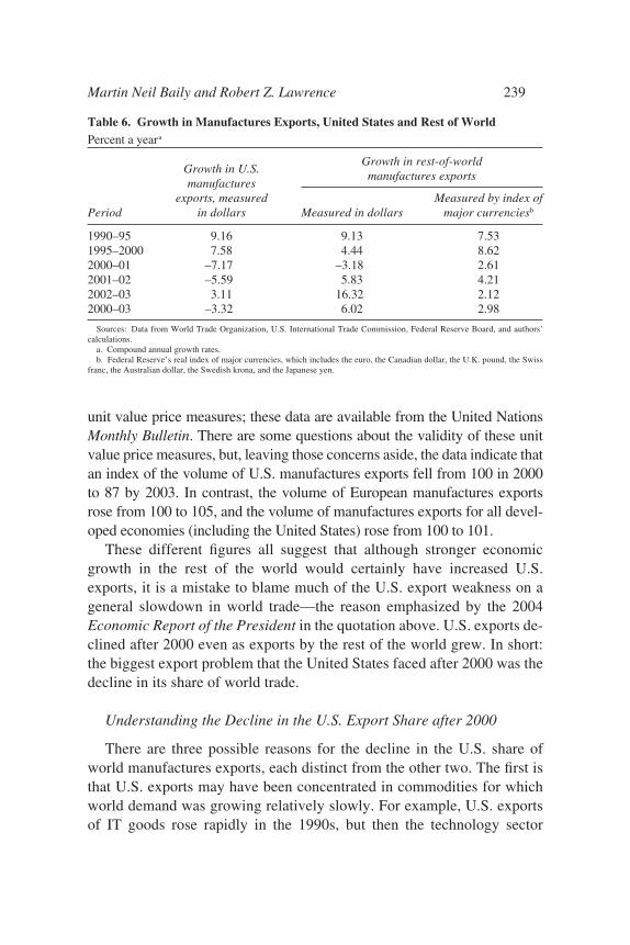
unit value price measures; these data are available from the United NationsMonthly Bulletin. There are some questions about the validity of these unitvalue price measures, but, leaving those concerns aside, the data indicate thatan index of the volume of U.S. manufactures exports fell from 100 in 2000to 87 by 2003. In contrast, the volume of European manufactures exportsrose from 100 to 105, and the volume of manufactures exports for all devel-oped economies (including the United States) rose from 100 to 101.

These different figures all suggest that although stronger economicgrowth in the rest of the world would certainly have increased U.S.exports, it is a mistake to blame much of the U.S. export weakness on ageneral slowdown in world trade—the reason emphasized by the 2004Economic Report of the President in the quotation above. U.S. exports de-clined after 2000 even as exports by the rest of the world grew. In short:the biggest export problem that the United States faced after 2000 was thedecline in its share of world trade.

Understanding the Decline in the U.S. Export Share after 2000

There are three possible reasons for the decline in the U.S. share ofworld manufactures exports, each distinct from the other two. The first isthat U.S. exports may have been concentrated in commodities for whichworld demand was growing relatively slowly. For example, U.S. exportsof IT goods rose rapidly in the 1990s, but then the technology sector


Table 6. Growth in Manufactures Exports, United States and Rest of WorldPercent a yeara

Growth in U.S.manufactures

exports, measured Measured by index ofPeriod in dollars Measured in dollars major currenciesb

1990–95 9.16 9.13 7.531995–2000 7.58 4.44 8.622000–01 –7.17 –3.18 2.612001–02 –5.59 5.83 4.212002–03 3.11 16.32 2.122000–03 –3.32 6.02 2.98

Sources: Data from World Trade Organization, U.S. International Trade Commission, Federal Reserve Board, and authors’calculations.

a. Compound annual growth rates.b. Federal Reserve’s real index of major currencies, which includes the euro, the Canadian dollar, the U.K. pound, the Swiss

franc, the Australian dollar, the Swedish krona, and the Japanese yen.

Growth in rest-of-worldmanufactures exports


slumped. The second possible reason is that U.S. exports may have gonemainly to countries that had particularly weak demand for imports duringthe period. And the third is that the United States may have lost competi-tiveness against other suppliers to the world market.

A standard approach to decomposing the trade data so as to capture theeffect of world trade growth and of the three sources of changes in the U.S.share of that growth is as follows:24 Let Vij be the value of U.S. exports ofcommodity i to country j in period 1, and V'ij the value of U.S. exports ofcommodity i to country j in period 2. Then we can define V and V' as follows:

In addition, let r be the percentage increase in total world exports fromperiod 1 to period 2, ri the percentage increase in world exports of com-modity i from period 1 to period 2, and rij the percentage increase in worldexports of commodity i to country j from period 1 to period 2. Then, asEdward Leamer and Robert Stern showed,25 the change in U.S. exportsfrom period 1 to period 2 can be expressed as follows:

The four terms on the right-hand side of this equation correspond to the fourcomponents described above. The first term reflects the change in U.S.exports that would occur if the United States simply maintained a constantshare of world trade. The second shows the extent to which U.S. tradechanges as a result of the commodity composition of U.S. exports. The thirdshows the extent to which U.S. trade changes as a result of the country com-position of U.S. exports. The final term is then the “competitiveness” term,although, when calculated as a residual, this term also includes the effect ofany additional factors not accounted for in the other terms.26

′ = + ( )

+ ( ) + ′( )∑ ∑ ∑∑ ∑∑V V rV r r V r r V V V r Vii

ijj

ij iji

ij ij ij ij ijji

– – – – – .

V V

V V

ijji

ijji

= =

′ = ′ =

∑∑∑∑

total U.S. exports in period 1

total U.S. exports in period 2.


24. Richardson (1970, 1971a, 1971b) has made important contributions to the litera-ture, while the discussion here is based on the exposition in Leamer and Stern (1970).

25. Leamer and Stern (1970).26. In implementing the decomposition we have made an adjustment to the standard

model, in line with the approach used earlier. In the equations shown above, world trade


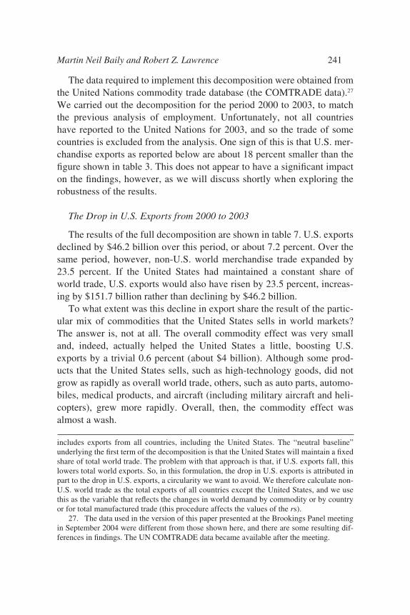
The data required to implement this decomposition were obtained fromthe United Nations commodity trade database (the COMTRADE data).27

We carried out the decomposition for the period 2000 to 2003, to matchthe previous analysis of employment. Unfortunately, not all countrieshave reported to the United Nations for 2003, and so the trade of somecountries is excluded from the analysis. One sign of this is that U.S. mer-chandise exports as reported below are about 18 percent smaller than thefigure shown in table 3. This does not appear to have a significant impacton the findings, however, as we will discuss shortly when exploring therobustness of the results.

The Drop in U.S. Exports from 2000 to 2003

The results of the full decomposition are shown in table 7. U.S. exportsdeclined by $46.2 billion over this period, or about 7.2 percent. Over thesame period, however, non-U.S. world merchandise trade expanded by23.5 percent. If the United States had maintained a constant share ofworld trade, U.S. exports would also have risen by 23.5 percent, increas-ing by $151.7 billion rather than declining by $46.2 billion.

To what extent was this decline in export share the result of the partic-ular mix of commodities that the United States sells in world markets?The answer is, not at all. The overall commodity effect was very smalland, indeed, actually helped the United States a little, boosting U.S.exports by a trivial 0.6 percent (about $4 billion). Although some prod-ucts that the United States sells, such as high-technology goods, did notgrow as rapidly as overall world trade, others, such as auto parts, automo-biles, medical products, and aircraft (including military aircraft and heli-copters), grew more rapidly. Overall, then, the commodity effect wasalmost a wash.


includes exports from all countries, including the United States. The “neutral baseline”underlying the first term of the decomposition is that the United States will maintain a fixedshare of total world trade. The problem with that approach is that, if U.S. exports fall, thislowers total world exports. So, in this formulation, the drop in U.S. exports is attributed inpart to the drop in U.S. exports, a circularity we want to avoid. We therefore calculate non-U.S. world trade as the total exports of all countries except the United States, and we usethis as the variable that reflects the changes in world demand by commodity or by countryor for total manufactured trade (this procedure affects the values of the rs).

27. The data used in the version of this paper presented at the Brookings Panel meetingin September 2004 were different from those shown here, and there are some resulting dif-ferences in findings. The UN COMTRADE data became available after the meeting.


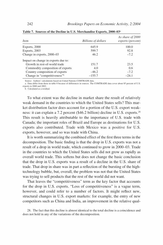
To what extent was the decline in market share the result of relativelyweak demand in the countries to which the United States sells? This mar-ket distribution factor does account for a portion of the U.S. export weak-ness: it can explain a 7.2 percent ($46.2 billion) decline in U.S. exports.28

This result is heavily attributable to the importance of U.S. trade withCanada; the important roles of Brazil and Europe as destinations for U.S.exports also contributed. Trade with Mexico was a positive for U.S.exports, however, and so was trade with China.

It is worth summarizing the combined effect of the first three terms in thedecomposition. The basic finding is that the drop in U.S. exports was not aresult of a drop in world trade, which continued to grow in 2000–03. Tradein the countries to which the United States sells did not grow as rapidly asoverall world trade. This softens but does not change the basic conclusionthat the drop in U.S. exports was a result of a decline in the U.S. share oftrade. That drop in share was in part a reflection of the bursting of the high-technology bubble, but, overall, the problem was not that the United Stateswas trying to sell products that the rest of the world did not want.

That leaves the “competitiveness” term as the key factor that accountsfor the drop in U.S. exports. “Loss of competitiveness” is a vague term,however, and could refer to a number of factors. It might reflect new,structural changes in U.S. export markets: for example, the entry of newcompetitors such as China and India, an improvement in the relative qual-


28. The fact that this decline is almost identical to the total decline is a coincidence anddoes not hold in any of the variations of the decomposition.

Table 7. Sources of the Decline in U.S. Merchandise Exports, 2000–03a

As share of 2000 Item Billions of dollars exports (percent)

Exports, 2000 645.9 100.0Exports, 2003 599.7 92.8Change in exports, 2000–03 46.2 –7.2

Impact on change in exports due to:Growth in rest-of-world trade 151.7 23.5Commodity composition of exports 4.0 0.6Country composition of exports –46.2 –7.2Change in “competitiveness”b –155.7 –24.1

Source: Authors’ calculations based on United Nations COMTRADE data.a. Data differ from those in table 8 because of differences in sources. The COMTRADE data cover about 85 percent of U.S.

exports in 2000 and 2003.b. Calculated as a residual.


ity of foreign goods, or a change in the sourcing patterns of U.S. multi-national corporations away from the United States toward other foreignlocations. However, such structural factors have been at work for sometime and seem unlikely to be the main reason for the rather abrupt shiftfrom rapid export growth in the 1990s to export decline in 2001 and 2002.

Any economic time series, of course, contains some random variation,and the “competitiveness” term includes any residual effects not capturedin the other terms of the decomposition, as well as any measurementerrors. U.S. exports grew unusually rapidly in 2000, perhaps a carryoverfrom export orders placed in the booming 1990s. Some decline, at least inthe growth of exports, might well have occurred even with unchangedeconomic conditions.

Finally, the competitiveness term may reflect the fact that U.S. goodsbecame relatively more expensive because of the behavior of the ex-change rate. The dollar strengthened against other major currencies in thelate 1990s and continued to do so until early 2002. The lagged effect ofthe sharp rise in the dollar was a major reason for the export decline in2000–03, as will be shown shortly.

We tested these results of the decomposition of the U.S. export declinefor robustness as follows. As we noted earlier, the calculations in table 6cover 2000–03 but omit some countries for which trade data are not avail-able. Data for a broader set of countries are available in the COMTRADEdatabase through 2002, and so we repeated the decomposition exercise forthe period 2000 to 2002, first using all available countries, and then onlythe countries for which data exist for 2003. Restricting the sample of coun-tries in this way made virtually no difference to the results of the decom-position for 2000–02, and so we infer that the same restriction in 2003 hasnot distorted the findings. Second, we excluded various commodities frommerchandise trade, such as energy products and items such as gold and“returned goods.” We also performed the decomposition for manufacturedgoods only. These variations again made very little difference to the re-sults, and therefore we have reported the findings for all merchandise tradefor comparability with the earlier employment calculations.

The Impact of the Dollar on U.S. Exports

To explore quantitatively the impact of changes in exchange rates, weused a rule-of-thumb framework based on empirical estimates of export



equations done by other researchers.29 We assume that 25 percent of theeffect of a change in the real dollar index on U.S. exports occurs in theyear after the devaluation, another 50 percent in the following year, andthe remaining 25 percent in the third year. The elasticity of U.S. exportsto changes in dollar exchange rates is assumed to be either 1.5 or 1.0.

We choose as our dollar index the real effective index of the dollaragainst major currencies, reported by the Federal Reserve Board. We usethis index because it seems reasonable to assume that U.S. exports com-pete primarily with the exports of other industrial countries. Table 8shows the impact of the dollar on U.S. merchandise exports from 2000 to2003, using the lag structure described above and the two alternative elas-ticities of demand for exports.

The first column of the table again shows the actual values of U.S. mer-chandise exports in 2000-03, based on official U.S. trade data. The secondcolumn shows what exports would have been if the rise in the dollar hadnot occurred (taking into account the lags). With an assumed elasticity of1.5, exports would have risen by $96.8 billion between 2000 and 2003,rather than falling by $54.8 billion as they did. The third and fourthcolumns show the impact on exports of the rise in the dollar, in dollarsand as a percentage of the total effect, respectively. The fifth column sim-ply repeats the figures given in table 4, showing the jobs due to exports,including the decline of 742,000 from 3.43 million in 2000 to 2.69 millionin 2003. The sixth column recalculates what these numbers would havebeen had the dollar’s exchange rate not changed over the period. Produc-tivity was growing fast enough that the number of jobs due to exportswould still have declined, but by only 183,000 instead of 742,000. As thelast column indicates, the U.S. economy would have had 559,000 addi-tional jobs due to exports if the dollar had remained unchanged, accordingto this analysis. This would have eliminated the loss of manufacturingjobs due to trade that we identified above.

A value of 1.5 for the exchange rate elasticity of exports is fairly high.If the true elasticity is smaller, the impact on exports and employment


29. See, for example, Houthakker and Magee (1969), Mahdavi (2000), Marquez (2002),Hooper, Johnson, and Marquez (1998), Mann (1999), Goldstein and Khan (1985), Senhadjiand Montenegro (1999), Stone (1979), Yang (1998), and Bailliu and Bouakez (2004).Although there are some outliers, results of most export equations fall within the range of1.0 to 1.5 for the long-run elasticity with a three-year lag. Most of the estimates are basedon prices rather than on the exchange rate, and so we assume 100 percent pass-through ofchanges in the exchange rate by U.S. exporters.


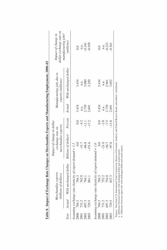
Tab

le 8

.Im

pact

of

Exc

hang

e R

ate

Cha

nges

on

Mer

chan

dise

Exp

orts

and

Man

ufac

turi

ng E

mpl

oym

ent,

200

0–03

Impa

ct o

f cha

nge

indo

llar

exc

hang

e ra

te o

nm

anuf

actu

ring

jobs

b

Yea

rA

ctua

lW

ith

unch

ange

d do

llar

Bil

lion

s of

dol

lars

aP

erce

ntA

ctua

lW

ith

unch

ange

d do

llar

(mil

lion

s)

Ass

umin

g ex

chan

ge r

ate

elas

tici

ty o

f exp

ort d

eman

d =

1.5

2000

784.

378

4.3

0.0

0.0

3.43

43.

434

0.0

2001

731.

276

2.9

–31.

7–4

.2n.

a.n.

a.n.

a.20

0269

7.3

784.

1–8

6.8

–11.

12.

739

3.08

0–0

.341

2003

729.

588

1.1

–151

.6–1

7.2

2.69

13.

250

–0.5

59

Ass

umin

g ex

chan

ge r

ate

elas

tici

ty o

f exp

ort d

eman

d =

1.0

2000

784.

378

4.3

0.0

0.0

3.43

43.

434

0.0

2001

731.

275

2.2

–21.

0–2

.8n.

a.n.

a.n.

a.20

0269

7.3

754.

0–5

6.7

–7.5

2.73

92.

961

–0.2

2320

0372

9.5

827.

3–9

7.8

–11.

82.

691

3.05

2–0

.361

Sou

rces

:D

ata

from

U.S

. Int

erna

tion

al T

rade

Com

mis

sion

, Bur

eau

of E

cono

mic

Ana

lysi

s, a

nd F

eder

al R

eser

ve B

oard

, and

aut

hors

’ ca

lcul

atio

ns.

a.D

iffe

renc

e be

twee

n ex

port

s w

ith

unch

ange

d do

llar

and

act

ual e

xpor

ts.

b.D

iffe

renc

e be

twee

n ex

port

jobs

wit

h un

chan

ged

doll

ar a

nd a

ctua

l exp

orts

.

Mer

chan

dise

exp

orts

(bil

lion

s of

dol

lars

)

Impa

ct o

f cha

nge

in d

olla

rex

chan

ge r

ate

on

mer

chan

dise

exp

orts

Man

ufac

turi

ng jo

bs d

ue to

expo

rts

(mil

lion

s)


will be proportionally lower. The corresponding calculations for an elas-ticity of 1.0 are shown in the bottom panel of table 8. According to the lastcolumn of that panel, under that assumption there would have been anadditional 361,000 jobs due to exports with an unchanged dollar. Again,the job loss due to trade would have been eliminated.

Conclusions

We conclude that the current and lagged effect of the rising dollar wasthe key reason for the weakness in U.S. exports after 2000. Strongergrowth in world trade would have helped U.S. exports, but the evidencepresented here indicates that the main factor contributing to this exportweakness was a decline in the U.S. share of world exports. The slump intrade in high-technology products lowered U.S. exports after 2000, butthis impact was largely offset by the relative strength of demand for theother goods that the United States sells in world markets. A number ofalternative explanations for the weakness of U.S. exports have been pre-sented by others. One is that the United States has lost competitivenessto China; a second is that U.S. multinational firms are increasinglysourcing their exports from foreign countries. But our analysis suggeststhat the impact of the stronger dollar is sufficient to account for most ofthe erosion in the U.S. share of trade in world markets and for the nega-tive impact of trade on employment.

The competitiveness effect reported in table 7 was $155.7 billion, butthat figure was derived from a database that excluded some countries.Simply scaling up that figure to make it comparable to table 8 gives acompetitiveness effect of $189.1 billion in 2003. With an elasticity of1.5 for the exchange rate, the rise in the dollar can explain fully 80 per-cent of this figure. It is thus by far the most compelling explanation ofthe weakness of U.S. exports and hence of the loss of manufacturing jobsdue to trade.

We have not tried to determine what explains the change in the dollarexchange rate. One plausible explanation is that the rapid growth associ-ated with the technology boom in the 1990s created investment opportu-nities that attracted capital to the United States. When the boom subsided,however, the lagged effects of the strong dollar on U.S. exports served tocompound the difficulties facing U.S. manufactures because of stagnantdomestic demand. As private capital flows subsided after 2000, they were



replaced to a large extent by foreign government purchases of U.S. assetsto keep the dollar high and reduce its rate of decline.

The Impact of Services Sector Offshoring to India on U.S. Jobs

The development of the business services sector in India, gearedheavily to exporting to the United States, has added a new layer of concern about the availability of good jobs in this country. The impactof trade on U.S. manufacturing jobs has been a matter of debate formany years, and one popular response has been to promote the benefitsof education. Low-skilled manual jobs in manufacturing are beingshifted overseas, it is argued, but American workers can still earn highwages provided they increase their level of skill and education. Theincrease in the return to education over the past twenty years has rein-forced this idea.

The rapid growth of services sector offshoring in India has rocked thisconventional wisdom.30 With large numbers of highly motivated, college-educated, English-speaking workers becoming available in India, in partthrough improved access to telecommunications capabilities, white-collarworkers in the United States now feel threatened.

This section explores the extent to which the weakness in job creationin the U.S. services sector during 2000–03, noted at the beginning of thispaper, can be attributed to the movement of service jobs to India. Hereas in the earlier discussion, we are well aware that, in a full, long-term,general equilibrium analysis there is no reason why an expansion oftrade should induce a loss of U.S. jobs in the aggregate. But getting asense of the number of jobs that may have been shifted from the UnitedStates to India is important to putting services sector offshoring in theright perspective.

Gauging the Impact of Offshoring to India

NASSCOM (National Association of Software and Service Compa-nies) is an Indian trade association that tracks the newly emerging busi-


30. There is now a large literature on the impact of offshoring: for example, Schultze(2004), Brainard and Litan (2004), Bhagwati, Panagariya, and Srinivasan (forthcoming),Baily and Farrell (2004), Atkinson (2004), and Bardhan and Kroll (2003).


ness services industry in that country.31 It collects data from Indian com-panies that provide IT services, such as computer programming, as wellas other business services (called business process offshoring or IT-enabled services) such as call centers and back office processing (forbanks and insurance companies, for example).

The initial impetus to the development of this industry came in partfrom General Electric Company, which in the 1990s saw the potential forcost savings from the availability of a skilled low-cost work force. In thepast, foreign companies operating in India, and even domestic companies,faced substantial barriers from the country’s maze of regulations and lackof infrastructure. Reliable electric power and telecommunications werenot readily available, and it took much time and persistence before Gen-eral Electric was able to start offshoring. The first movers were foreignmultinationals like General Electric and the U.K.-based HSBC Group, butthe industry has shifted over time so that local companies such as Daksh,Spectramind, Infosys, and Wipro have contributed to the growth in recentyears. It remains the case, however, that two-thirds of the industry con-sists of captive producers (those owned by or affiliated with foreign multi-nationals, many of them U.S. and British companies).

The first column of table 9 shows that, over the period from NASSCOM’s 2000/01 fiscal year to its 2003/04 fiscal year (NASSCOM’sfiscal year ends with the first quarter), software employment in Indiaincreased by 200,000 workers. Of these, 134,000 were involved in ser-vices exported to the United States. On the assumption that this workwould have required the same number of employees in the UnitedStates—that is, that the productivity of the U.S. and Indian softwareindustries are the same, this implies a transfer of 134,000 U.S. jobs.

The second column of table 9 shows a comparable computation forbusiness process offshoring. Employment in these activities in Indiaincreased by 175,500 workers, 140,400 of whom produced services thatwere exported to the United States. Again assuming a one-for-one jobtransfer, this means a loss of 140,400 U.S. jobs in this service activity.

The assumption of comparable productivity is a strong one. Some whohave studied the Indian industry and visited its facilities report that the


31. A description of NASSCOM and a variety of data series are available on the orga-nization’s website. This section uses information collected as part of the McKinsey GlobalInstitute (2003) case study of India offshoring.


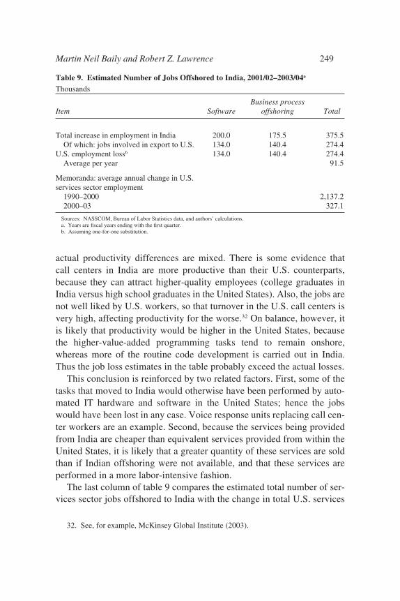
actual productivity differences are mixed. There is some evidence thatcall centers in India are more productive than their U.S. counterparts,because they can attract higher-quality employees (college graduates inIndia versus high school graduates in the United States). Also, the jobs arenot well liked by U.S. workers, so that turnover in the U.S. call centers isvery high, affecting productivity for the worse.32 On balance, however, itis likely that productivity would be higher in the United States, becausethe higher-value-added programming tasks tend to remain onshore,whereas more of the routine code development is carried out in India.Thus the job loss estimates in the table probably exceed the actual losses.

This conclusion is reinforced by two related factors. First, some of thetasks that moved to India would otherwise have been performed by auto-mated IT hardware and software in the United States; hence the jobswould have been lost in any case. Voice response units replacing call cen-ter workers are an example. Second, because the services being providedfrom India are cheaper than equivalent services provided from within theUnited States, it is likely that a greater quantity of these services are soldthan if Indian offshoring were not available, and that these services areperformed in a more labor-intensive fashion.

The last column of table 9 compares the estimated total number of ser-vices sector jobs offshored to India with the change in total U.S. services


32. See, for example, McKinsey Global Institute (2003).

Table 9. Estimated Number of Jobs Offshored to India, 2001/02–2003/04a

Thousands

Business processItem Software offshoring Total

Total increase in employment in India 200.0 175.5 375.5Of which: jobs involved in export to U.S. 134.0 140.4 274.4

U.S. employment lossb 134.0 140.4 274.4Average per year 91.5

Memoranda: average annual change in U.S. services sector employment

1990–2000 2,137.22000–03 327.1

Sources: NASSCOM, Bureau of Labor Statistics data, and authors’ calculations.a. Years are fiscal years ending with the first quarter.b. Assuming one-for-one substitution.


sector employment. Summing the estimates for the software and businessprocess industries suggests that at most about 275,000 jobs moved toIndia over the three-year period 2000/01 to 2003/04, for an annual aver-age change of about 91,500 jobs. For the displaced workers the costs ofthis increase in trade were surely substantial, but a job shift of this size isvery small compared with the 2.1 million service jobs created in theUnited States in a typical year during the 1990s; it is even small comparedwith the net annual increase from 2000 to 2003, when annual service jobcreation fell to about 327,000.

Comparing the NASSCOM Data with U.S. Services Trade Data

According to the Bureau of Economic Analysis (BEA), total U.S. ser-vices trade with India is very small, and indeed the United States actuallyruns a surplus. Moreover, total U.S. services imports from India actuallydeclined between 2000 and 2002. (“Services trade” refers to private ser-vices trade unless stated otherwise.) The BEA data, shown in figure 6,indicate that services imports from India rose fairly strongly from 1995 to2000, more than doubling in current dollars from about $850 million to$1.90 billion, but subsequently fell back to $1.84 billion in 2002. Servicesexports to India have been consistently larger than services imports fromIndia, according to the BEA, and have grown very rapidly over time,especially after 1999. Exports in 2002 are reported as $3.28 billion.

The BEA data do not indicate the nature of the services that are traded,but the discrepancy with the NASSCOM data is already clear. Accordingto NASSCOM, IT and business process services exports from India to theUnited States were around $6 billion in 2002, more than triple the BEA’sfigure for total U.S. services imports from India in that year. There areseveral reasons why the BEA data may understate imports from India, andwhy the NASSCOM data may overstate exports to the United States.Most likely both errors are occurring. But, before we dissect this discrep-ancy, it is worth noting one important inference to be drawn from theBEA data. As already noted, the United States is not simply an importerof services from India; it is also a significant and growing exporter of ser-vices to India. As the Indian economy grows, it is likely to provide anincreasing market for U.S. services and to contribute to job creation inservices industries where the United States has a comparative advantage.The analysis of offshoring presented above leaves out this part of theemployment effects of services trade between the two countries.



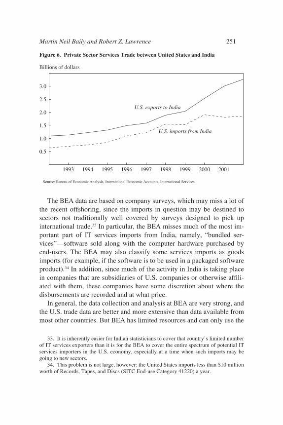
The BEA data are based on company surveys, which may miss a lot ofthe recent offshoring, since the imports in question may be destined tosectors not traditionally well covered by surveys designed to pick upinternational trade.33 In particular, the BEA misses much of the most im-portant part of IT services imports from India, namely, “bundled ser-vices”—software sold along with the computer hardware purchased byend-users. The BEA may also classify some services imports as goodsimports (for example, if the software is to be used in a packaged softwareproduct).34 In addition, since much of the activity in India is taking placein companies that are subsidiaries of U.S. companies or otherwise affili-ated with them, these companies have some discretion about where thedisbursements are recorded and at what price.

In general, the data collection and analysis at BEA are very strong, andthe U.S. trade data are better and more extensive than data available frommost other countries. But BEA has limited resources and can only use the


33. It is inherently easier for Indian statisticians to cover that country’s limited numberof IT services exporters than it is for the BEA to cover the entire spectrum of potential ITservices importers in the U.S. economy, especially at a time when such imports may begoing to new sectors.

34. This problem is not large, however: the United States imports less than $10 millionworth of Records, Tapes, and Discs (SITC End-use Category 41220) a year.

Figure 6. Private Sector Services Trade between United States and India

0.5

1.0

1.5

2.0

2.5

3.0

1993 1994 1995 1996 1997 1998 1999 2000 2001

Source: Bureau of Economic Analysis, International Economic Accounts, International Services.

Billions of dollars

U.S. exports to India

U.S. imports from India


data available to it from existing surveys, which were not set up to moni-tor services sector offshoring from India. There is a large overall statisti-cal discrepancy in the international accounts, which makes it evident thatnot all international transactions are captured. The magnitude and timepattern of the BEA data on services imports from India also seem totallyout of line with the rapid growth and development of the IT and businessprocess industries, located in India and serving the U.S. market, which isvisible to Indians themselves and to journalists and researchers from theUnited States.

The most important reason why the NASSCOM data may exaggerateIndia’s exports is that some fraction of the software services provided bycompanies reporting to NASSCOM is performed by employees who areactually located in the United States—for example, the work of program-mers on assignment to and located in the United States may be counted asIndian exports if they are working under contract to a company based inIndia. NASSCOM itself states on its website that 40 percent of its ITactivities are associated with personnel located at the customer’s site.BEA Director Steven Landefeld has noted that the payments made tothese persons would not be counted as imports to the United States, nor inhis view should they be.35 If this view is correct, we should scale back thenumbers given earlier by 40 percent for the IT jobs. The estimate of thesoftware jobs transferred would drop from 134,000 over three years to80,400.

We chose not to scale back the earlier estimates, however, for the fol-lowing reasons. First, applying the 40 percent figure for Indian personnellocated in the United States seems inconsistent with U.S. visa datareported by the Department of Homeland Security (or the Immigrationand Naturalization Service). In particular, the number of Indians on H1-Bvisas (issued to workers in specialty occupations) in the United States wasonly 81,000 (47,500 of whom worked in computer-related fields) in 2002,and indeed was lower than the level in 2000. The number on L-1 visas(intercompany transfers) was only 20,400 and had also fallen since 2000.On this evidence it seems that the number of Indians transferred to U.S.companies has been falling since 2000, not rising, which makes it veryhard to attribute any of the growth in employment reported in the NASSCOM employment data to increases in persons working in the


35. Steven Landefeld, personal communication with the authors, April 7, 2004.


United States. Perhaps the H1-B and L-1 visa data are missing a lot ofpeople, but we know that entering the United States has become muchmore difficult since September 2001. Either a lot of employees of Indiancompanies have green cards or U.S. citizenship, or the 40 percent figure iswrong.36

The second reason is that this paper is exploring the decline in U.S.payroll employment. If Indian workers employed by establishmentslocated in India are being assigned to projects located in U.S. companies’domestic facilities, these workers will not show up on the U.S. payrollsurvey.37 They are not on the payroll of a U.S. company. From the per-spective of understanding U.S. payroll employment, it is appropriate tocount these jobs as having been offshored to Indian workers and com-panies, regardless of how their salaries either are or should be counted inthe U.S. balance of trade data.

Finally, and most important, the purpose of this exercise is to show thatthe offshoring of services sector jobs to India, so far, has been small com-pared with total services sector employment in the United States. If theNASSCOM data do overstate the magnitude of offshoring, then that con-clusion will hold even more strongly. The NASSCOM data on the off-shoring of services from the United States then provide an upper boundon the actual value of U.S. services imports and on the number of jobspreviously performed in the United States that are now being performedin India.

U.S. Employment in Occupations Likelyto Have Been Affected by Offshoring

Given the enormous size of the services sector in the United States(about 110 million workers in 2004), it is not really a surprise to find thatservices sector offshoring to India so far has not been large in relation tototal U.S. services employment. But it is certainly possible that theimpact on the U.S. labor market of the growth of the Indian industry hasbeen larger for IT and IT-enabled occupations. Our conclusion is that,yes, offshoring to India has been large enough to have had some impacton IT jobs in the United States. However, we find that employment in the


36. Thus far we have not been able to receive clarification from NASSCOM about thevalidity of the 40 percent figure.

37. This was confirmed by a phone conversation with Bureau of Labor Statistics staff.


IT sector has actually been surprisingly strong in the past few years,especially if one allows for the unsustainable surge in employment in2000.

Table 10 uses data from the OES, described above, with a focus onemployment patterns between 1999 and 2003 in those occupations thatmay have been affected by offshoring.38 Looking first at the computer-related services occupations (top panel of table 10), we find only a mod-est drop in total employment—about 65,500 over 2000–03, or about 2.5percent.39 Moreover, as Catherine Mann has pointed out, the employ-ment decline after 2000 followed a huge technology boom in the late1990s, which culminated in a surge of employment and investmentaimed at resolving the Y2K problem.40 The employment levels reachedin 2000 were not sustainable, regardless of what happened to U.S. ser-vices trade with India. As one sign of this, employment in computeroccupations was actually over 230,000 higher in 2003 than it had beenin 1999 (the earliest year for which these data are available). The shorttime period makes it impossible to be sure of the trends, but the figuresfor 1999–2003 tentatively suggest an underlying trend toward increas-ing employment in computer occupations over the period, with a tem-porary surge in 2000 that was followed by a temporary downwardadjustment.

The table does show some shift in the mix of employment within com-puter occupations. The biggest job losers were computer programmersand computer support personnel, about 139,000 of whom lost jobs over2000–03. Among computer support personnel there was a large surge inemployment between 1999 and 2000, strongly suggesting a Y2K effect.Employment in 2003 remained above the level in 1999.

For computer programmers, however, the decline in employment couldhave been the result of offshoring to India. Table 10 shows a decline of99,090 in U.S. computer programming jobs from 2000 to 2003. Our esti-mate of IT jobs in India in table 9 suggests that as many as 134,000 suchjobs were created in India to serve the United States. Our estimate of the


38. The table is adapted from similar tables in Mann (2003) and Kirkegaard (2004). Wehave benefited from their analysis of high-technology employment.

39. The analysis in this section does not include production workers in the IT hardwareindustry. We showed above that manufacturing employment in the computer and semi-conductor industries fell very sharply after 2000.

40. Mann (2003).


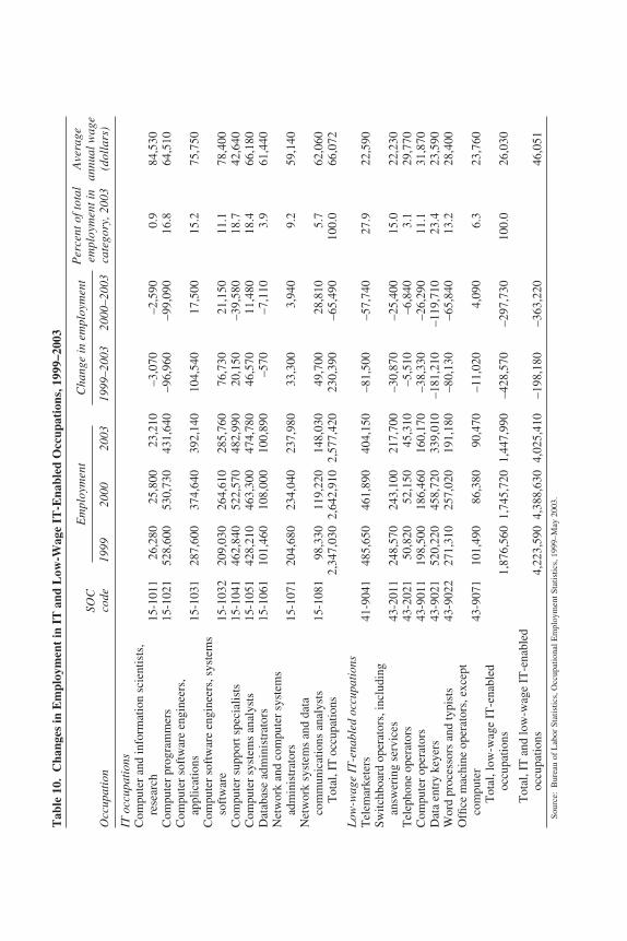
Tab

le 1

0.C

hang

es in

Em

ploy

men

t in

IT

and

Low

-Wag

e IT

-Ena

bled

Occ

upat

ions

, 199

9–20

03

Per

cent

of t

otal

Ave

rage

SOC

empl

oym

ent i

nan

nual

wag

eO

ccup

atio

nco

de19

9920

0020

0319

99–2

003

2000

–200

3ca

tego

ry, 2

003

(dol

lars

)

IT o

ccup

atio

nsC

ompu

ter

and

info

rmat

ion

scie

ntis

ts,

rese

arch

15-1

011

26,2

8025

,800

23,2

10–3

,070

–2,5

900.

984

,530

Com

pute

r pr

ogra

mm

ers

15-1

021

528,

600

530,

730

431,

640

–96,

960

–99,

090

16.8

64,5

10C

ompu

ter

soft

war

e en

gine

ers,

ap

plic

atio

ns15

-103

128

7,60

037

4,64

039

2,14

010

4,54

017

,500

15.2

75,7

50C

ompu

ter

soft

war

e en

gine

ers,

sys

tem

s

soft

war

e15

-103

220

9,03

026

4,61

028

5,76

076

,730

21,1

5011

.178

,400

Com

pute

r su

ppor

t spe

cial

ists

15-1

041

462,

840

522,

570

482,

990

20,1

50–3

9,58

018

.742

,640

Com

pute

r sy

stem

s an

alys

ts15

-105

142

8,21

046

3,30

047

4,78

046

,570

11,4

8018

.466

,180

Dat

abas

e ad

min

istr

ator

s15

-106

110

1,46

010

8,00

010

0,89

0–5

70–7

,110

3.9

61,4

40N

etw

ork

and

com

pute

r sy

stem

s

adm

inis

trat

ors

15-1

071

204,

680

234,

040

237,

980

33,3

003,

940

9.2

59,1

40N

etw

ork

syst

ems

and

data

co

mm

unic

atio

ns a

naly

sts

15-1

081

98,3

3011

9,22

014

8,03

049

,700

28,8

105.

762

,060

Tot

al, I

T o

ccup

atio

ns2,

347,

030

2,64

2,91

02,

577,

420

230,

390

–65,

490

100.

066

,072

Low

-wag

e IT

-ena

bled

occ

upat

ions

Tel

emar

kete

rs41

-904

148

5,65

046

1,89

040

4,15

0–8

1,50

0–5

7,74

027

.922

,590

Switc

hboa

rd o

pera

tors

, inc

ludi

ng

answ

erin

g se

rvic

es43

-201

124

8,57

024

3,10

021

7,70

0–3

0,87

0–2

5,40

015

.022

,230

Tel

epho

ne o

pera

tors

43-2

021

50,8

2052

,150

45,3

10–5

,510

–6,8

403.

129

,770

Com

pute

r op

erat

ors

43-9

011

198,

500

186,

460

160,

170

–38,

330

–26,

290

11.1

31,8

70D

ata

entr

y ke

yers

43-9

021

520,

220

458,

720

339,

010

–181

,210

–119

,710

23.4

23,5

90W

ord

proc

esso

rs a

nd ty

pist

s43

-902

227

1,31

025

7,02

019

1,18

0–8

0,13

0–6

5,84

013

.228

,400

Offi

ce m

achi

ne o

pera

tors

, exc

ept

com

pute

r43

-907

110

1,49

086

,380

90,4

70–1

1,02

04,

090

6.3

23,7

60T

otal

, low

-wag

e IT

-ena

bled

oc

cupa

tions

1,87

6,56

01,

745,

720

1,44

7,99

0–4

28,5

70–2

97,7

3010

0.0

26,0

30

Tot

al, I

T a

nd lo

w-w

age

IT-e

nabl

ed

occu

patio

ns4,

223,

590

4,38

8,63

04,

025,

410

–198

,180

–363

,220

46,0

51S

ourc

e:B

urea

u of

Lab

or S

tati

stic

s, O

ccup

atio

nal E

mpl

oym

ent S

tati

stic

s, 1

999–

May

200

3.

Em

ploy

men

tC

hang

e in

em

ploy

men

t


shift of jobs to India is probably too high, but nevertheless these figuresindicate the possibility that the loss of U.S. programming jobs was theresult of a movement of work to India.

As already noted, comparative advantage within the computer pro-gramming sector may have led, as trade with India became cheaper andeasier, to basic programming tasks being offshored while the higher-endactivities continued to expand in the United States. Between 2000 and2003 there were increases in the employment of computer softwareengineers (applications and systems) even as employment of computerprogrammers declined. The same holds even more strongly from 1999to 2003.

In short, the availability of low-cost programming services from Indiasurely has had an impact on the U.S. software industry. Indeed, onewould expect such an impact, because U.S. customers benefit from theeffects of the input price reduction generated by the availability of low-cost programmers.

The benefits from increased services trade will be reduced if such traderesults in the permanent loss of U.S. human capital. This would occur iftrained programmers in the United States were never reemployed or weremoved to jobs that did not make use of the programming skills they hadacquired. Press accounts provide anecdotal evidence that some U.S.workers have indeed experienced such a loss of human capital. Althoughthis situation is attributable in part to offshoring, there were also mis-perceptions in the late 1990s about the sustainability of the technologyboom.

In addition, the employment data in table 10 suggest that the loss ofjobs in the technology sector was actually relatively small over all. Giventhe slump in the U.S. technology sector and in the domestic demand forIT, it is actually very surprising that employment in computer occupationsfell so little between 2000 and 2003 and that it remains well above the1999 employment level.

The bottom panel of table 10 shows that IT-enabled low-wage occu-pations, such as telemarketers, computer operators, and word proces-sors, experienced substantial employment declines—nearly 300,000over the 2000–03 period and well over 400,000 from 1999 through2003. The declines occurred across the board in these occupations, andsome were probably due to activities being shifted overseas. In othercases, however, technology was the culprit. For example, employment



of word processors has declined in part because most office workersnow carry out that function themselves on personal computers insteadof using dictation or handwritten material. Similarly, computer opera-tors are not needed in the same numbers because of the shift away frommainframes.

It is noteworthy that wages for these occupations are not very high—inthe $10 to $15 an hour range. That is certainly better than the minimumwage, but not so high that alternative jobs at similar pay would be difficultto find in most urban labor markets. Voluntary turnover rates are alsofairly high among positions at that level. As discussed previously, thissuggests that human capital losses would be limited. We do not wish tominimize the personal cost borne by those whose jobs are shifted over-seas, but the adjustment cost of this offshoring to the labor market as awhole should not be very high.

Conclusions

Even under assumptions that may greatly overstate the offshoring ofservices sector jobs to India, we find that press reports and popular dis-cussion of the issue greatly exaggerate its importance to the U.S. labormarket. The evidence so far suggests that the number of jobs transferredto India is tiny relative to total employment in the U.S. services sector.Within computer occupations, we find that the net job loss for computerprogrammers in the United States is likely attributable to offshoring.However, the surprising fact is how little employment in computer ser-vices has fallen in recent years, given the weakness in U.S. domesticdemand for technology services.

The Impact of Expected Future Offshoring in Services

One possible rejoinder to this conclusion is that what has happened sofar may be minor, but that in the future the offshoring of services sectorjobs will affect the U.S. labor market more severely. We explore that pos-sibility next.

The debate over the effects of electronic offshoring in the long run hasreflected a variety of concerns. A recent paper by Jagdish Bhagwati, ArvindPanagariya, and T. N. Srinivasan considers the impact of offshoring on



welfare.41 A second issue is the impact of electronic outsourcing on thestructure of U.S. employment. In the short run the United States may runlarger trade deficits as a result of the increase in services sector off-shoring, but over the long run any increase in services imports will haveto be paid for by additional net exports—that is, by exporting more goodsand services or reducing imports of other goods and services. Thus,although outsourcing could mean fewer services jobs in some sectors, itcould also mean more jobs in other sectors that produce tradable goodsand services.

In this analysis the first question to be addressed is, How large is out-sourcing likely to be? Although any forecast of the future magnitude ofservices sector offshoring is subject to great uncertainty, the most fre-quently quoted figures, those compiled by Forrester Research, suggestthat 3.4 million U.S. service jobs will be offshored to India and othercountries by 2015.42 These estimates derive from a series of companyinterviews in both the United States and India. Forrester attempted toassess which U.S. occupations were amenable to offshoring, what skillswere available overseas, and what investments were being made orplanned to develop capabilities overseas.43

The Forrester study finds that 315,000 service jobs had already beenoffshored by 2003 and that an additional 3.1 million jobs would move off-shore by 2015—hence the estimated total of 3.4 million. By far the largestoccupational category affected is office workers, accounting for nearlyhalf of the jobs offshored. But the study further suggests that a range ofpossible employment categories could be offshored, including computer,business, management, and sales workers, and workers in architectureand the life sciences.44

Although one should not place undue confidence in the Forrester num-bers, they are sufficiently interesting for their implications to be explored.Moreover, in different simulation runs, we used some alternative assump-tions about the magnitude of offshoring. The results were roughly linear,so that those who believe that the true number of offshored jobs will behalf as great, or twice as great, as our estimates can simply halve or dou-


41. Bhagwati, Panagariya, and Srinivasan (fothcoming); Samuelson (2004).42. McCarthy and others (forthcoming).43. McCarthy and others (2004, p. 4).44. McCarthy and others (2004, p. 5).


ble the results reported here to get a first approximation of the impact onthe economy.

To formulate the simulations, we worked with Ben Herzon and JoelPrakken of Macroeconomic Advisers (MA) to see how the level of off-shoring predicted by Forrester would affect the economy. The difficultpart of this analysis is to capture in a sensible fashion the impact of the“shock” imparted to the economy by the rapid increase in services sectoroffshoring. We experimented with various approaches and will report thetwo that, together, provide the most helpful insights. The impact of off-shoring is inferred from the deviations of our “offshoring” simulationsfrom MA’s baseline simulation; therefore we begin by offering a sense ofwhat the baseline looks like.

The Baseline Scenario

MA’s long-term simulations do not attempt to capture cyclical variationsof the economy more than a few quarters out. This is standard practice forsuch forecasting models, for example those of the Council of EconomicAdvisers and the Office of Management and Budget, as well as the economicassumptions used by the Congressional Budget Office in its budget forecast-ing. The baseline simulation embodies an implicit Federal Reserve reactionfunction that ensures that, in the absence of shocks, the economy remainsclose to full employment, assumed to be consistent with an unemploymentrate of around 5.3 percent. The baseline used for this paper uses actual datathrough the first quarter of 2004 and thus does not reflect the increases in oilprices and the weakening of the U.S. economy that occurred in mid-2004(what Federal Reserve Chairman Alan Greenspan has referred to as a “softpatch”). In this baseline the U.S. economy continues its cyclical recovery,and the unemployment rate falls to its target range by the end of 2004.

These characteristics of the baseline, together with the gradual, smoothramp-up of offshoring that is built into the Forrester estimates, mean thatfor our purposes there is little significant information to be obtained fromthe quarter-to-quarter changes in the economic variables. We compare thestarting point of the baseline (in the first quarter of 2004) with the endpoint in the fourth quarter of 2015. The variables move relativelysmoothly during the intermediate years.

When the MA model is run without adjustments, it predicts continuinglarge current account deficits for the United States. However, MA’s current



thinking is that these large deficits are not sustainable and that the dollarwill decline substantially over the next ten years or so.45 The baseline sim-ulation therefore shows a gradual decline in the dollar of around 21 percentand a reduction of the U.S. current account deficit to around $100 billion,or 0.5 percent of the predicted $20 trillion current-dollar U.S. GDP in2015:4. The downward adjustment of the current account, accompaniedby a shift in real net exports from negative to positive, is accomplishedwithout imposing excessively high interest rates, because a substantialreduction in the federal budget deficit is assumed over the same period.The baseline thus builds in a rather smooth resolution of the two bigdeficit problems facing today’s economy.

Table 11 reports the values for a range of variables in the starting andending quarters of the baseline and their growth rates when appropriate.Over the nearly twelve-year forecast period, real GDP grows at 2.9 per-cent a year and inflation averages a bit under 2.0 percent a year. Nonfarmpayroll employment rises at 0.9 percent a year over the period, and laborproductivity growth in the nonfarm business sector is 2.3 percent a year.The decline in the dollar contributes to strong growth of real U.S. non-farm merchandise exports, at a rate of 7.3 percent a year; real servicesexport growth is similar. Since trend productivity growth in the manufac-turing sector is less than 7.3 percent a year, the implied growth of realexports would contribute positively to manufacturing employment in thisbaseline simulation. The baseline simulation implies that trade willincrease manufacturing employment going forward. Real nonpetroleumimports are dampened by the fall in the dollar and grow at 5.6 percent ayear. Real petroleum imports (not shown) grow even more slowly. Realservices imports in the baseline are also dampened by the dollar declineand by rising prices, and they grow relatively slowly.

The baseline projections can be combined with our estimates ofemployment due to exports and imports in 2003, reported in table 4, toprovide estimates of changes in employment due to trade between 2003and 2015. To do this, it is necessary to make an assumption about whatrate of labor productivity growth in manufacturing would be associatedwith a 2.3 percent annual average growth rate for nonfarm business out-


45. It is notoriously difficult to model exchange rate determination econometrically; inparticular, it is very difficult to capture the downward pressure on the dollar that will likelycome about (and in part has already come about) as dollar assets rise as a share of the port-folio of the rest of the world.


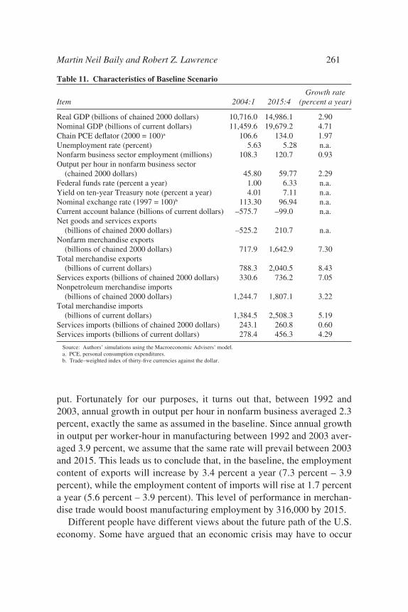
put. Fortunately for our purposes, it turns out that, between 1992 and2003, annual growth in output per hour in nonfarm business averaged 2.3percent, exactly the same as assumed in the baseline. Since annual growthin output per worker-hour in manufacturing between 1992 and 2003 aver-aged 3.9 percent, we assume that the same rate will prevail between 2003and 2015. This leads us to conclude that, in the baseline, the employmentcontent of exports will increase by 3.4 percent a year (7.3 percent – 3.9percent), while the employment content of imports will rise at 1.7 percenta year (5.6 percent – 3.9 percent). This level of performance in merchan-dise trade would boost manufacturing employment by 316,000 by 2015.

Different people have different views about the future path of the U.S.economy. Some have argued that an economic crisis may have to occur


Table 11. Characteristics of Baseline Scenario

Growth rateItem 2004:1 2015:4 (percent a year)

Real GDP (billions of chained 2000 dollars) 10,716.0 14,986.1 2.90Nominal GDP (billions of current dollars) 11,459.6 19,679.2 4.71Chain PCE deflator (2000 = 100)a 106.6 134.0 1.97Unemployment rate (percent) 5.63 5.28 n.a.Nonfarm business sector employment (millions) 108.3 120.7 0.93Output per hour in nonfarm business sector

(chained 2000 dollars) 45.80 59.77 2.29Federal funds rate (percent a year) 1.00 6.33 n.a.Yield on ten-year Treasury note (percent a year) 4.01 7.11 n.a.Nominal exchange rate (1997 = 100)b 113.30 96.94 n.a.Current account balance (billions of current dollars) –575.7 –99.0 n.a.Net goods and services exports

(billions of chained 2000 dollars) –525.2 210.7 n.a.Nonfarm merchandise exports

(billions of chained 2000 dollars) 717.9 1,642.9 7.30Total merchandise exports

(billions of current dollars) 788.3 2,040.5 8.43Services exports (billions of chained 2000 dollars) 330.6 736.2 7.05Nonpetroleum merchandise imports

(billions of chained 2000 dollars) 1,244.7 1,807.1 3.22Total merchandise imports

(billions of current dollars) 1,384.5 2,508.3 5.19Services imports (billions of chained 2000 dollars) 243.1 260.8 0.60Services imports (billions of current dollars) 278.4 456.3 4.29

Source: Authors’ simulations using the Macroeconomic Advisers’ model.a. PCE, personal consumption expenditures.b. Trade–weighted index of thirty-five currencies against the dollar.


before the nation’s deficit problems will be resolved. Terrorism or othershocks could disrupt economic growth. Others argue that large U.S. cur-rent account or budget deficits, or both, can continue indefinitely. How-ever, the MA baseline looks exactly right for the purpose here. We wantto abstract from other economic issues and focus on the impact of off-shoring. To what extent services sector offshoring might interact withother shocks we leave to others to determine.

The Macroeconomic Effect of Services Sector Offshoring: Adding More Imports

One simple way to model the impact of services offshoring is toimpose on the model an increase in the demand for services imports. Weasked MA to adjust the services import equation so as to shift the demandcurve outward. Using the Forrester employment data and the U.S. wage-cost numbers as a basis, we estimated what the increase in imports wouldbe, under the assumption that the imported services would cost only halfas much as supplying the equivalent services domestically.46

If the dollar exchange rate is left unchanged, the increase in importstranslates into an increased current account deficit. We judged that a moreneutral comparison with the baseline would result from imposing an addi-tional decline in the dollar as a result of the increased offshoring, in orderto keep the current account balance the same as in the baseline.

Table 12 summarizes the results of this simulation. The model trans-lates the increase in imports into an immediate negative shock to GDP,which Federal Reserve policy must offset in order to preserve employ-ment. Over time, however, the greater decline in the dollar stimulatesexports and slows real import growth. By the end of the simulation run,the dollar is 7.5 below its baseline level, and this has increased real mer-chandise exports and reduced real merchandise imports. The lower dollarhas pushed inflation up a little and pushed up interest rates. With thehigher interest rates there is a slight reduction in productivity growth, andreal GDP is down very slightly by 2015 compared with the baseline. In


46. The 50 percent figure is our estimate based on McKinsey Global Institute (2003). Ifanything, the cost would be somewhat less than 50 percent—in the 45 to 50 percent range.It is possible that the relative cost calculation would change over time as the foreign indus-try expands. However, Indian businesses are expanding their operations outside of theircurrent region, to avoid rising labor costs, and other countries are investing in the infra-structure and language training that would allow them to enter the market.


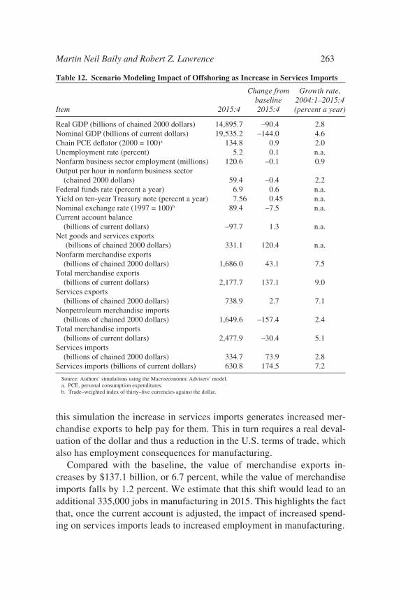
this simulation the increase in services imports generates increased mer-chandise exports to help pay for them. This in turn requires a real deval-uation of the dollar and thus a reduction in the U.S. terms of trade, whichalso has employment consequences for manufacturing.

Compared with the baseline, the value of merchandise exports in-creases by $137.1 billion, or 6.7 percent, while the value of merchandiseimports falls by 1.2 percent. We estimate that this shift would lead to anadditional 335,000 jobs in manufacturing in 2015. This highlights the factthat, once the current account is adjusted, the impact of increased spend-ing on services imports leads to increased employment in manufacturing.


Table 12. Scenario Modeling Impact of Offshoring as Increase in Services Imports

Change from Growth rate,baseline 2004:1–2015:4

Item 2015:4 2015:4 (percent a year)

Real GDP (billions of chained 2000 dollars) 14,895.7 –90.4 2.8Nominal GDP (billions of current dollars) 19,535.2 –144.0 4.6Chain PCE deflator (2000 = 100)a 134.8 0.9 2.0Unemployment rate (percent) 5.2 0.1 n.a.Nonfarm business sector employment (millions) 120.6 –0.1 0.9Output per hour in nonfarm business sector

(chained 2000 dollars) 59.4 –0.4 2.2Federal funds rate (percent a year) 6.9 0.6 n.a.Yield on ten-year Treasury note (percent a year) 7.56 0.45 n.a.Nominal exchange rate (1997 = 100)b 89.4 –7.5 n.a.Current account balance

(billions of current dollars) –97.7 1.3 n.a.Net goods and services exports

(billions of chained 2000 dollars) 331.1 120.4 n.a.Nonfarm merchandise exports

(billions of chained 2000 dollars) 1,686.0 43.1 7.5Total merchandise exports

(billions of current dollars) 2,177.7 137.1 9.0Services exports

(billions of chained 2000 dollars) 738.9 2.7 7.1Nonpetroleum merchandise imports

(billions of chained 2000 dollars) 1,649.6 –157.4 2.4Total merchandise imports

(billions of current dollars) 2,477.9 –30.4 5.1Services imports

(billions of chained 2000 dollars) 334.7 73.9 2.8Services imports (billions of current dollars) 630.8 174.5 7.2

Source: Authors’ simulations using the Macroeconomic Advisers’ model.a. PCE, personal consumption expenditures.b. Trade–weighted index of thirty–five currencies against the dollar.


In summary, this simulation run, modeled as a case in which the UnitedStates has effectively developed an increased taste for services imports,results in a modest negative for the economy: inflation, productivity, andthe terms of trade are all negatively affected. The job displacement hap-pens slowly, based on the Forrester assessment, and this allows FederalReserve policy to maintain full employment. The MA model is a generalequilibrium model, and it predicts that most of the workers displacedfrom their jobs will find new ones. There is a predicted boost to manufac-turing employment, although overall employment is essentially the samein this simulation run as it is in the baseline.

The Macroeconomic Effect of Services Sector Offshoring: A Declinein the Price of Services Imports

The previous simulation is a useful starting point, but it does not reflectthe underlying economics of services sector offshoring. What is theunderlying shock that triggers the increased offshoring that Forrester pre-dicts? Presumably, it is that improved technology and infrastructure com-bined with capital and training have lowered the price that the UnitedStates pays for services sector imports. As a result, the United States buysmore of them. For any given value of the dollar, the decline in importprices improves the U.S. terms of trade.

With offshoring, U.S. companies find they can produce the same levelof sales or gross output with fewer domestic workers. Initially, theirprofitability rises as they sell at the same price domestically with reducedcosts (they pay only 50 percent of the cost for the activities they off-shore). Over time, however, competition works to lower prices and dis-tributes the benefits back to consumers. Productivity rises within thecompanies doing the offshoring. They buy more foreign inputs but savelabor, and, since they have reduced their costs, their productivity ishigher. Productivity rises for the U.S. economy as a whole if the workersand capital displaced by the increased services imports are reemployedin activities that generate more than enough real output to pay for theincrease in real services imports.

In order to capture this process, MA adjusted the price of servicesimports down by an amount large enough to induce an increase in the realquantity of services imports that, in turn, was large enough to displace thenumber of workers that Forrester predicts will be displaced. In the samequarter in which the increased offshoring takes place, there is a drop in



payroll employment and a rise in productivity and corporate profits. Overtime, domestic prices fall and Federal Reserve policy acts to restoreemployment. Domestic workers who are displaced are reabsorbed into theeconomy, according the normal dynamics built into the MA model.

Table 13 summarizes the results of the simulations. Offshoring of themagnitude suggested by Forrester is enough to add 0.2 percentage point toannual GDP growth and nearly 0.3 percentage point a year to growth inlabor productivity in the nonfarm business sector. Real GDP is $384 bil-lion higher by 2015. Total employment and unemployment are essentiallythe same as in the baseline. The inflation rate has been lowered by 0.25 percentage point a year, even though the dollar is down 4.8 percent.

As one would expect, real services imports are higher in this simula-tion, but services imports in current dollars are actually slightly lower.The fall in the price of imports means that the United States can buy morereal imports for the same dollar cost. The decline in the dollar partiallyoffsets the opening up of the low-cost offshoring opportunity.47

Table 13 shows that the values of merchandise exports and importsboth rise—by $101.6 billion and $63.5 billion, respectively—relative tothe baseline. In this scenario manufacturing employment due to tradeincreases by 62,000. In both simulations, therefore, more services importsimplies more jobs in manufacturing over the long run.

The idea that offshoring could raise U.S. productivity and hence U.S.GDP is not a surprise. That is, after all, what we expect to be the benefit ofexpanded trade. The magnitude of the increments to these variables, how-ever, is larger than we anticipated. It is not easy to determine how changesin variables play out through the structure of a large macroeconomicmodel, but it seems that the reason for the “multiplier effect” of off-shoring on real GDP is that the Federal Reserve follows a path of lowerinterest rates in this simulation. It does that because domestic labor isbeing released as a result of the job displacement and because inflation islower as a result of the cheaper services imports. In the MA model thelower interest rates have a positive impact on domestic investment, andthis contributes to the growth in productivity and hence in GDP.


47. The decline in the dollar increases merchandise exports in these results. That resultis plausible enough, but it was not robust across the different model runs. The MA model’sprice equations capture relative price effects between traded goods and services prices andthe price of domestic production. Depending on the specification, these effects can elimi-nate the increase in merchandise exports.


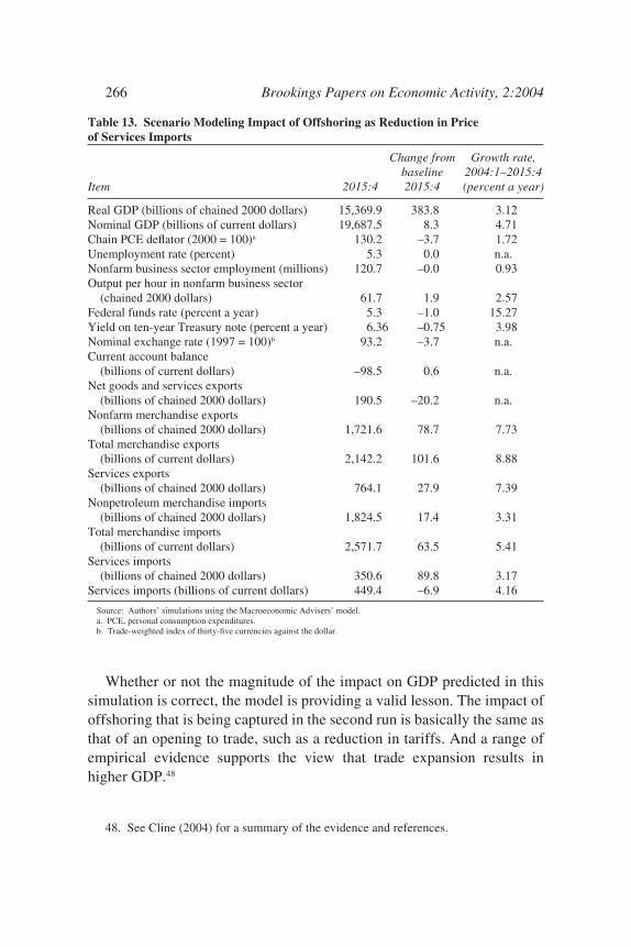
Whether or not the magnitude of the impact on GDP predicted in thissimulation is correct, the model is providing a valid lesson. The impact ofoffshoring that is being captured in the second run is basically the same asthat of an opening to trade, such as a reduction in tariffs. And a range ofempirical evidence supports the view that trade expansion results inhigher GDP.48


Table 13. Scenario Modeling Impact of Offshoring as Reduction in Price of Services Imports

Change from Growth rate,baseline 2004:1–2015:4

Item 2015:4 2015:4 (percent a year)

Real GDP (billions of chained 2000 dollars) 15,369.9 383.8 3.12Nominal GDP (billions of current dollars) 19,687.5 8.3 4.71Chain PCE deflator (2000 = 100)a 130.2 –3.7 1.72Unemployment rate (percent) 5.3 0.0 n.a.Nonfarm business sector employment (millions) 120.7 –0.0 0.93Output per hour in nonfarm business sector

(chained 2000 dollars) 61.7 1.9 2.57Federal funds rate (percent a year) 5.3 –1.0 15.27Yield on ten-year Treasury note (percent a year) 6.36 –0.75 3.98Nominal exchange rate (1997 = 100)b 93.2 –3.7 n.a.Current account balance

(billions of current dollars) –98.5 0.6 n.a.Net goods and services exports

(billions of chained 2000 dollars) 190.5 –20.2 n.a.Nonfarm merchandise exports

(billions of chained 2000 dollars) 1,721.6 78.7 7.73Total merchandise exports

(billions of current dollars) 2,142.2 101.6 8.88Services exports

(billions of chained 2000 dollars) 764.1 27.9 7.39Nonpetroleum merchandise imports

(billions of chained 2000 dollars) 1,824.5 17.4 3.31Total merchandise imports

(billions of current dollars) 2,571.7 63.5 5.41Services imports

(billions of chained 2000 dollars) 350.6 89.8 3.17Services imports (billions of current dollars) 449.4 –6.9 4.16

Source: Authors’ simulations using the Macroeconomic Advisers’ model.a. PCE, personal consumption expenditures.b. Trade-weighted index of thirty-five currencies against the dollar.

48. See Cline (2004) for a summary of the evidence and references.


Wages and Profits

The simulation runs on the MA model do not tell us anything about thedistribution of wages across different types of workers, but they do makea prediction about total wages (or rather, total compensation of employ-ees) and profits. Table 14 reports the findings. The simulation in whichthe services import equation was add-factored up showed a negativeeffect on the economy, and table 14 indicates that this loss is imposed onemployees. Real compensation is reduced by nearly $160 billion by 2015,or 1.9 percent. Profits remain essentially unaffected in this simulation.

In contrast, the simulation in which the price of imports is reducedresults in benefits to the economy, and these are shared by labor and capital. Real compensation is increased by $209 billion and profits by$142 billion. The increase in profits is much larger in percentage terms(11.4 percent) than the increase in compensation (2.5 percent). Off-shoring in this simulation thus shifts the distribution of income towardcapital. In this simulation the initial impact of offshoring is to increaseprofits and displace labor. Over time, however, competition and higherproductivity result in lower prices, and that is what increases real com-pensation. But higher profits are a persistent consequence of the ongoingprocess of offshoring. It is not surprising to find that, if the U.S. econ-omy becomes more exposed to low-cost labor, the result will be to shiftthe distribution of income toward capital. Employees as a whole are bet-ter off in this simulation, however.

Conclusion

We began by pointing to the large and sustained drop in payrollemployment that followed the end of the 1990s boom, and we presented avariety of evidence to suggest that trade and offshoring were not majorreasons for this decline. The weakness in U.S. exports did contribute tothe job loss, however.

What, then, is the main explanation of the weakness in employment?Charles Schultze has argued that the main cause is rapid productivitygrowth.49 We agree that rapid productivity growth may be playing some


49. Schultze (2004).


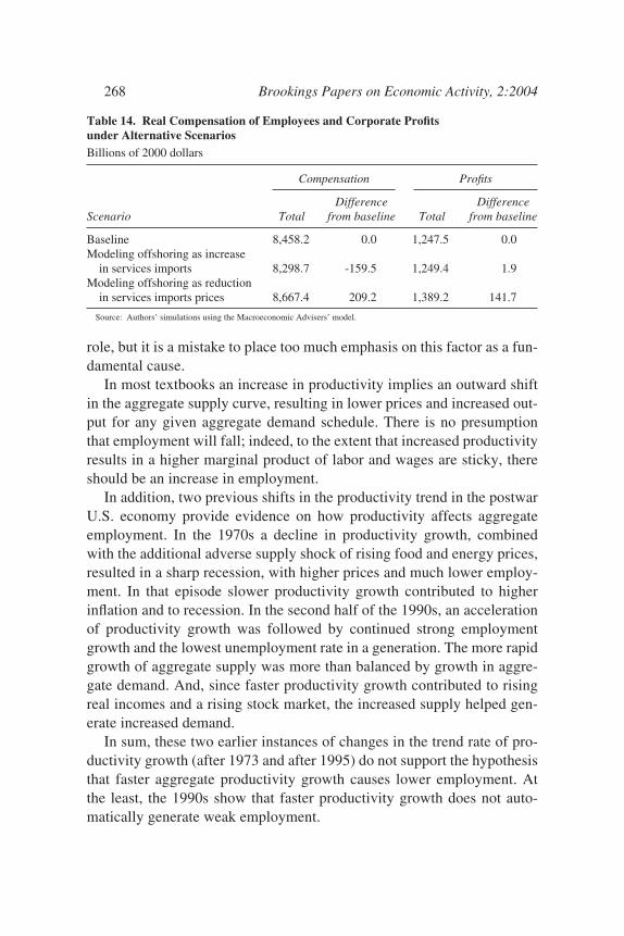
role, but it is a mistake to place too much emphasis on this factor as a fun-damental cause.

In most textbooks an increase in productivity implies an outward shiftin the aggregate supply curve, resulting in lower prices and increased out-put for any given aggregate demand schedule. There is no presumptionthat employment will fall; indeed, to the extent that increased productivityresults in a higher marginal product of labor and wages are sticky, thereshould be an increase in employment.

In addition, two previous shifts in the productivity trend in the postwarU.S. economy provide evidence on how productivity affects aggregateemployment. In the 1970s a decline in productivity growth, combinedwith the additional adverse supply shock of rising food and energy prices,resulted in a sharp recession, with higher prices and much lower employ-ment. In that episode slower productivity growth contributed to higherinflation and to recession. In the second half of the 1990s, an accelerationof productivity growth was followed by continued strong employmentgrowth and the lowest unemployment rate in a generation. The more rapidgrowth of aggregate supply was more than balanced by growth in aggre-gate demand. And, since faster productivity growth contributed to risingreal incomes and a rising stock market, the increased supply helped gen-erate increased demand.

In sum, these two earlier instances of changes in the trend rate of pro-ductivity growth (after 1973 and after 1995) do not support the hypothesisthat faster aggregate productivity growth causes lower employment. Atthe least, the 1990s show that faster productivity growth does not auto-matically generate weak employment.


Table 14. Real Compensation of Employees and Corporate Profits under Alternative ScenariosBillions of 2000 dollars

Compensation Profits

Difference DifferenceScenario Total from baseline Total from baseline

Baseline 8,458.2 0.0 1,247.5 0.0Modeling offshoring as increase

in services imports 8,298.7 -159.5 1,249.4 1.9Modeling offshoring as reduction

in services imports prices 8,667.4 209.2 1,389.2 141.7

Source: Authors’ simulations using the Macroeconomic Advisers’ model.


Rapid productivity growth after 2000 did raise the bar, however. Itmeant that aggregate demand would have had to grow strongly in order tomaintain employment growth, and that did not occur. With strongly ex-pansionary monetary and fiscal policies, the recession of 2001 was verymild, and the employment drop was not unusual. The puzzle has been thefailure of demand and employment to recover strongly enough after 2001.The reasons for this include the uncertainty resulting from 9/11 and thewar in Iraq, the direct effect of higher oil prices, the overhang from theinvestment boom of the late 1990s, the weakness of the stock market(only partly offset by the recovery in 2003), and, as we have emphasized,the lagged impact of the strong dollar in the aftermath of the Asian finan-cial crisis. The drop in U.S. capital goods investment, and notably thedecline in the demand for high-technology products, contributed to theweakness of manufacturing employment. Monetary and fiscal policies,although expansionary, were not powerful enough to offset these nega-tives. Fiscal policy was more effective at increasing the budget deficitthan at spurring demand. Monetary policy was about as expansionary as itcould be, and it certainly helped sustain demand for housing and automo-biles. But history suggests that low interest rates can have a limitedimpact on aggregate demand in the presence of business and consumeruncertainty, especially given the lower bound on nominal interest rates.

We do not suggest that the U.S. economy is mired in perpetual jobweakness, however. The economy has repeatedly demonstrated its abilityto recover, and we expect aggregate demand and employment to increasegoing forward, barring a new oil shock or major terrorist attack or othercalamity.

Since trade and offshoring were not the main reasons for the em-ployment weakness, they should not be the focus of policies to restoreemployment. Likewise, since imports were not the reason for the job loss,there is not an employment case for trade restrictions to curtail imports.

Instead the best trade-related remedy for manufacturing employment is a lower value of the dollar and a sustained recovery of the world economy—outcomes that are desirable for other reasons as well. In the late1990s, when domestic demand in the United States was booming, thestrong dollar helped relieve pressures on the U.S. labor market by reducingexports and stimulating imports. It would certainly have been inadvisableand inflationary for the United States to have reduced interest rates in aneffort to weaken the dollar in 1999 and 2000. However, once the economy



fell into a recession, the lagged impact of the strong dollar contributed tolabor market weakness.

U.S. policymakers have limited power to affect the exchange rate ofthe dollar and the strength of the world economy. However, once theoverall recovery is well established, a sustained effort to reduce the fed-eral budget deficit would help lower interest rates and reduce the over-valuation of the dollar—and would be good policy in any case. Policiesthat might ameliorate the adverse effects of job reallocation caused bytrade include, in our judgment, trade adjustment assistance programs andopportunities for workers to improve their skill levels.



Comments andDiscussion

Frank Levy: About the time I received this paper, my wife and I had to drive our daughter to college. Because her room needed a floor lamp,we ended up at IKEA. The reader can already see where this story isheading. The floor lamp was nice, functional if not high style, andadjustable in height up to about six feet. It was made in China and cost$9.95. I informally sampled other IKEA items and found many had sim-ilarly low prices.

I appreciate the distinction between anecdotes and data, but having justseen these extremely low prices, I found this paper by Martin Baily andRobert Lawrence quite timely. The paper draws four principal conclusions:

—The substantial loss of manufacturing jobs since 2000 was primar-ily a function of weak aggregate domestic demand, not due to a flood ofimports.

—To the extent that trade did cause manufacturing job losses, it did sothrough a sharp decline in exports. This decline can be largely explainedby the rise in the dollar, which undercut U.S. competitiveness.

—The outsourcing of service jobs was not particularly large in scale,either in information technology services or in clerical back office work.

—If, however, the Forrester Research predictions of future outsourcingwere to come true, the resulting job losses would be substantial. These joblosses would not pose a threat to full employment, but, under a variety ofassumptions, they would shift the composition of national income awayfrom wages and toward capital.

In this comment I will discuss first the jobs data and then the paper’sanalysis of the data. I will end by summarizing what the reader shouldtake away from the paper.

271


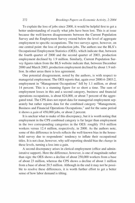
To explain the loss of jobs since 2000, it would be helpful first to get abetter understanding of exactly what jobs have been lost. This is at issuebecause the well-known disagreements between the Current PopulationSurvey and the Employment Survey extend below the level of aggregateemployment to specific occupations. The two surveys agree, however, onone central point: the loss of production jobs. The authors use the BLS’sOccupational Employment Statistics (OES), which indicate that, betweenthe fourth quarter of 2000 and the second quarter of 2003, productionemployment declined by 1.9 million. Similarly, Current Population Sur-vey figures taken from the BLS website indicate that, between December2000 and March 2003, production employment declined by about 1.9 mil-lion. In other areas there is less agreement.

One potential disagreement, noted by the authors, is with respect tomanagerial employment. The OES reports that, again over 2000:4–2003:2,employment in “Management Occupations” fell by 1.1 million, or about14 percent. This is a stunning figure for so short a time. The sum ofemployment losses in this and a second category, business and financialoperations occupations, is about 824,000, or about 7 percent of the aggre-gated total. The CPS does not report data for managerial employment sep-arately but rather reports data for the combined category “Management,Business and Financial Operations Occupations,” and for the same periodit shows a gain of 458,000 jobs, or about 2 percent.

It is unclear what to make of this discrepancy, but it is worth noting thatemployment in the CPS combined category is far larger than employmentin the two corresponding categories in the OES: roughly 19.6 millionworkers versus 12.4 million, respectively, in 2000. As the authors note,some of this difference in levels reflects the well-known bias in the house-hold survey due to respondents’ tendency to inflate their occupationaltitles. It is not clear, however, why self-reporting should bias the change inthese levels, turning a loss into a gain.

A second discrepancy arises in clerical employment (office and admin-istrative support). Here the difference, however, is one of magnitude ratherthan sign: the OES shows a decline of about 250,000 workers from a baseof about 23 million, whereas the CPS shows a decline of about 1 millionfrom a base of about 20.5 million. Although in the end it may not be possi-ble to resolve these differences, it is worth further effort to get a bettersense of how labor demand is tilting.



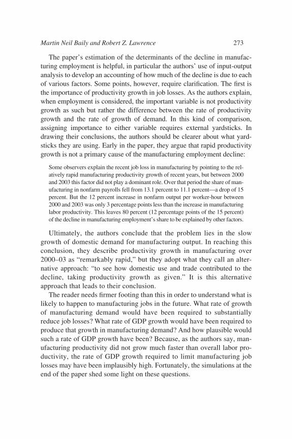
The paper’s estimation of the determinants of the decline in manufac-turing employment is helpful, in particular the authors’ use of input-outputanalysis to develop an accounting of how much of the decline is due to eachof various factors. Some points, however, require clarification. The first isthe importance of productivity growth in job losses. As the authors explain,when employment is considered, the important variable is not productivitygrowth as such but rather the difference between the rate of productivitygrowth and the rate of growth of demand. In this kind of comparison,assigning importance to either variable requires external yardsticks. Indrawing their conclusions, the authors should be clearer about what yard-sticks they are using. Early in the paper, they argue that rapid productivitygrowth is not a primary cause of the manufacturing employment decline:

Some observers explain the recent job loss in manufacturing by pointing to the rel-atively rapid manufacturing productivity growth of recent years, but between 2000and 2003 this factor did not play a dominant role. Over that period the share of man-ufacturing in nonfarm payrolls fell from 13.1 percent to 11.1 percent—a drop of 15percent. But the 12 percent increase in nonfarm output per worker-hour between2000 and 2003 was only 3 percentage points less than the increase in manufacturinglabor productivity. This leaves 80 percent (12 percentage points of the 15 percent)of the decline in manufacturing employment’s share to be explained by other factors.

Ultimately, the authors conclude that the problem lies in the slowgrowth of domestic demand for manufacturing output. In reaching thisconclusion, they describe productivity growth in manufacturing over2000–03 as “remarkably rapid,” but they adopt what they call an alter-native approach: “to see how domestic use and trade contributed to thedecline, taking productivity growth as given.” It is this alternativeapproach that leads to their conclusion.

The reader needs firmer footing than this in order to understand what islikely to happen to manufacturing jobs in the future. What rate of growthof manufacturing demand would have been required to substantiallyreduce job losses? What rate of GDP growth would have been required toproduce that growth in manufacturing demand? And how plausible wouldsuch a rate of GDP growth have been? Because, as the authors say, man-ufacturing productivity did not grow much faster than overall labor pro-ductivity, the rate of GDP growth required to limit manufacturing joblosses may have been implausibly high. Fortunately, the simulations at theend of the paper shed some light on these questions.



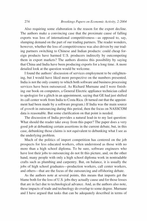
Also requiring some elaboration is the reason for the export decline.The authors make a convincing case that the proximate cause of fallingexports was loss of international competitiveness—as opposed to, say,slumping demand on the part of our trading partners. The reader wonders,however, whether the loss of competitiveness was also driven by our trad-ing partners switching to Chinese and Indian products: could cheap for-eign products have harmed U.S. producers indirectly by outcompetingthem in export markets? The authors dismiss this possibility by sayingthat China and India have been producing exports for a long time. A moredetailed look at the question would be welcome.

I found the authors’ discussion of services employment to be enlighten-ing, but I would have liked more perspective on the numbers presented.India is not the only country to which both software and business processingservices have been outsourced. As Richard Murnane and I were finish-ing our book on computers, a General Electric appliance technician calledto apologize for a glitch in an appointment, saying that GE had just shiftedits call center work from India to Costa Rica. (It turned out that the appoint-ment had been made by a software program.) If India was the main sourceof growth in outsourcing during this period, then the focus on NASSCOMdata is reasonable. But some clarification on that point is needed.

The discussion of India provides a natural lead-in to my last question:What should the reader take away from this paper? The paper does a verygood job at debunking certain assertions in the current debate, but, in thiscase, debunking those claims is not equivalent to debunking what I see asthe underlying problem.

Much of the politics of import competition has centered on the jobprospects for less educated workers, often understood as those with nomore than a high school diploma. To be sure, software engineers whohave lost their jobs to outsourcing do not fit this picture, and, on the otherhand, many people with only a high school diploma work in nontradablecrafts such as plumbing and carpentry. But, on balance, it is usually thejobs of high school graduates—production workers, call center workers,and others—that are the focus of the outsourcing and offshoring debate.

As the authors note at several points, this means that imports get theblame both for the loss of U.S. jobs they actually cause and for those lossesthat are in fact due to technological advance. And, as the authors also note,these impacts of trade and technology do overlap to some degree. Murnaneand I have argued that tasks that can be adequately described in terms of



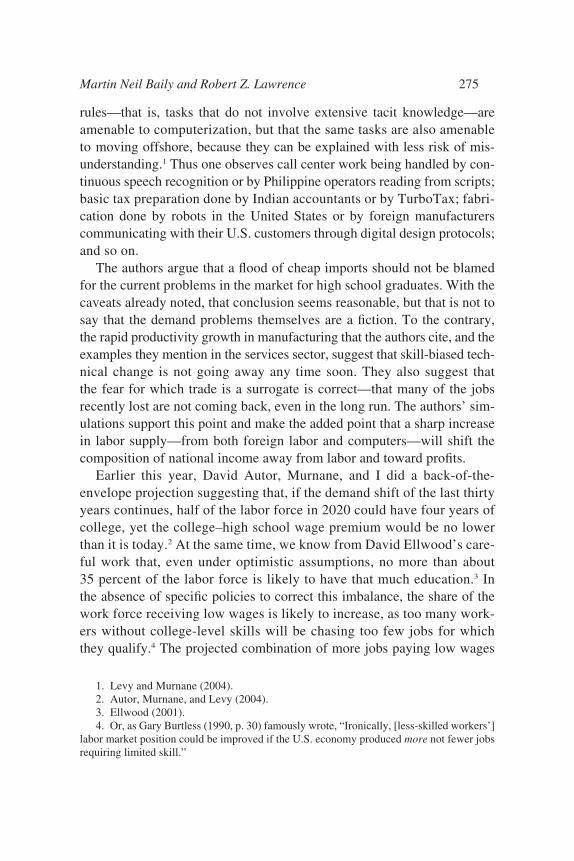
rules—that is, tasks that do not involve extensive tacit knowledge—areamenable to computerization, but that the same tasks are also amenableto moving offshore, because they can be explained with less risk of mis-understanding.1 Thus one observes call center work being handled by con-tinuous speech recognition or by Philippine operators reading from scripts;basic tax preparation done by Indian accountants or by TurboTax; fabri-cation done by robots in the United States or by foreign manufacturerscommunicating with their U.S. customers through digital design protocols;and so on.

The authors argue that a flood of cheap imports should not be blamedfor the current problems in the market for high school graduates. With thecaveats already noted, that conclusion seems reasonable, but that is not tosay that the demand problems themselves are a fiction. To the contrary,the rapid productivity growth in manufacturing that the authors cite, and theexamples they mention in the services sector, suggest that skill-biased tech-nical change is not going away any time soon. They also suggest that the fear for which trade is a surrogate is correct—that many of the jobsrecently lost are not coming back, even in the long run. The authors’ sim-ulations support this point and make the added point that a sharp increasein labor supply—from both foreign labor and computers—will shift thecomposition of national income away from labor and toward profits.

Earlier this year, David Autor, Murnane, and I did a back-of-the-envelope projection suggesting that, if the demand shift of the last thirtyyears continues, half of the labor force in 2020 could have four years ofcollege, yet the college–high school wage premium would be no lowerthan it is today.2 At the same time, we know from David Ellwood’s care-ful work that, even under optimistic assumptions, no more than about 35 percent of the labor force is likely to have that much education.3 Inthe absence of specific policies to correct this imbalance, the share of thework force receiving low wages is likely to increase, as too many work-ers without college-level skills will be chasing too few jobs for whichthey qualify.4 The projected combination of more jobs paying low wages


1. Levy and Murnane (2004).2. Autor, Murnane, and Levy (2004).3. Ellwood (2001).4. Or, as Gary Burtless (1990, p. 30) famously wrote, “Ironically, [less-skilled workers’]

labor market position could be improved if the U.S. economy produced more not fewer jobsrequiring limited skill.”


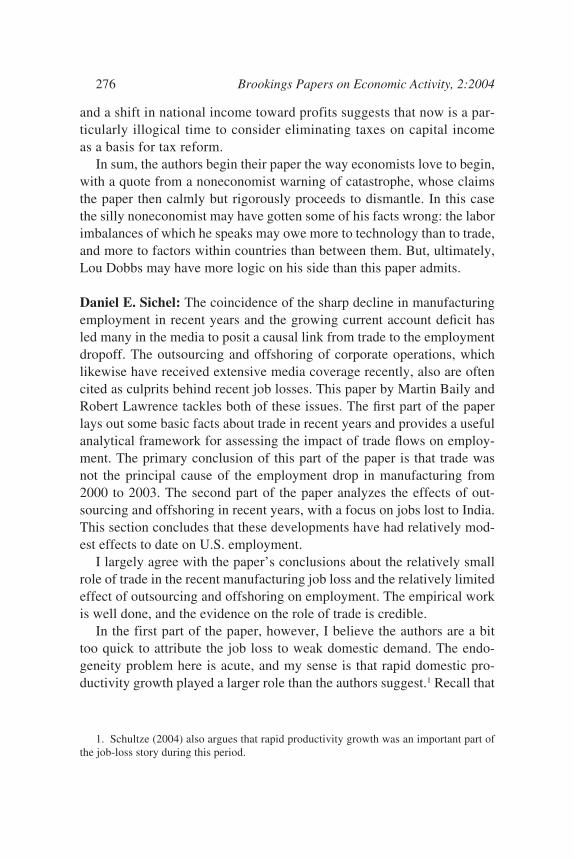
and a shift in national income toward profits suggests that now is a par-ticularly illogical time to consider eliminating taxes on capital incomeas a basis for tax reform.

In sum, the authors begin their paper the way economists love to begin,with a quote from a noneconomist warning of catastrophe, whose claimsthe paper then calmly but rigorously proceeds to dismantle. In this casethe silly noneconomist may have gotten some of his facts wrong: the laborimbalances of which he speaks may owe more to technology than to trade,and more to factors within countries than between them. But, ultimately,Lou Dobbs may have more logic on his side than this paper admits.

Daniel E. Sichel: The coincidence of the sharp decline in manufacturingemployment in recent years and the growing current account deficit hasled many in the media to posit a causal link from trade to the employmentdropoff. The outsourcing and offshoring of corporate operations, whichlikewise have received extensive media coverage recently, also are oftencited as culprits behind recent job losses. This paper by Martin Baily andRobert Lawrence tackles both of these issues. The first part of the paperlays out some basic facts about trade in recent years and provides a usefulanalytical framework for assessing the impact of trade flows on employ-ment. The primary conclusion of this part of the paper is that trade wasnot the principal cause of the employment drop in manufacturing from2000 to 2003. The second part of the paper analyzes the effects of out-sourcing and offshoring in recent years, with a focus on jobs lost to India.This section concludes that these developments have had relatively mod-est effects to date on U.S. employment.

I largely agree with the paper’s conclusions about the relatively smallrole of trade in the recent manufacturing job loss and the relatively limitedeffect of outsourcing and offshoring on employment. The empirical workis well done, and the evidence on the role of trade is credible.

In the first part of the paper, however, I believe the authors are a bittoo quick to attribute the job loss to weak domestic demand. The endo-geneity problem here is acute, and my sense is that rapid domestic pro-ductivity growth played a larger role than the authors suggest.1 Recall that


1. Schultze (2004) also argues that rapid productivity growth was an important part ofthe job-loss story during this period.


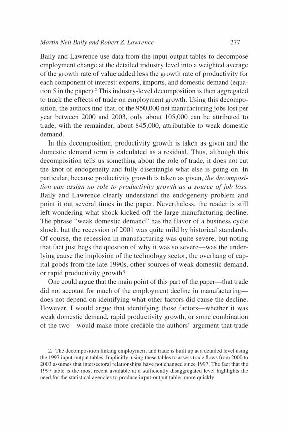
Baily and Lawrence use data from the input-output tables to decomposeemployment change at the detailed industry level into a weighted averageof the growth rate of value added less the growth rate of productivity foreach component of interest: exports, imports, and domestic demand (equa-tion 5 in the paper).2 This industry-level decomposition is then aggregatedto track the effects of trade on employment growth. Using this decompo-sition, the authors find that, of the 950,000 net manufacturing jobs lost peryear between 2000 and 2003, only about 105,000 can be attributed totrade, with the remainder, about 845,000, attributable to weak domesticdemand.

In this decomposition, productivity growth is taken as given and thedomestic demand term is calculated as a residual. Thus, although thisdecomposition tells us something about the role of trade, it does not cutthe knot of endogeneity and fully disentangle what else is going on. Inparticular, because productivity growth is taken as given, the decomposi-tion can assign no role to productivity growth as a source of job loss.Baily and Lawrence clearly understand the endogeneity problem andpoint it out several times in the paper. Nevertheless, the reader is stillleft wondering what shock kicked off the large manufacturing decline.The phrase “weak domestic demand” has the flavor of a business cycleshock, but the recession of 2001 was quite mild by historical standards.Of course, the recession in manufacturing was quite severe, but notingthat fact just begs the question of why it was so severe—was the under-lying cause the implosion of the technology sector, the overhang of cap-ital goods from the late 1990s, other sources of weak domestic demand,or rapid productivity growth?

One could argue that the main point of this part of the paper—that tradedid not account for much of the employment decline in manufacturing—does not depend on identifying what other factors did cause the decline.However, I would argue that identifying those factors—whether it wasweak domestic demand, rapid productivity growth, or some combinationof the two—would make more credible the authors’ argument that trade


2. The decomposition linking employment and trade is built up at a detailed level usingthe 1997 input-output tables. Implicitly, using these tables to assess trade flows from 2000 to2003 assumes that intersectoral relationships have not changed since 1997. The fact that the1997 table is the most recent available at a sufficiently disaggregated level highlights theneed for the statistical agencies to produce input-output tables more quickly.


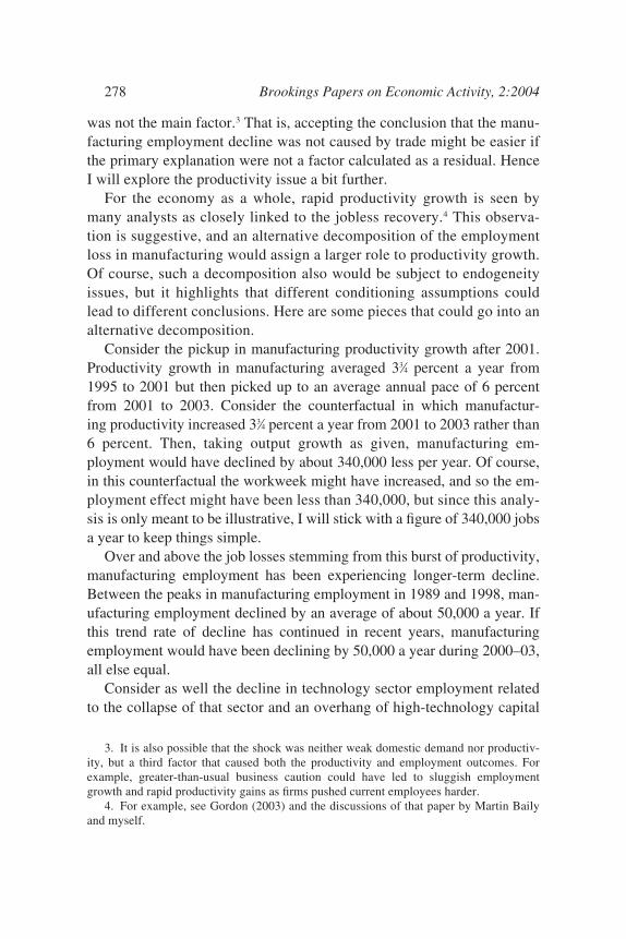
was not the main factor.3 That is, accepting the conclusion that the manu-facturing employment decline was not caused by trade might be easier ifthe primary explanation were not a factor calculated as a residual. HenceI will explore the productivity issue a bit further.

For the economy as a whole, rapid productivity growth is seen bymany analysts as closely linked to the jobless recovery.4 This observa-tion is suggestive, and an alternative decomposition of the employmentloss in manufacturing would assign a larger role to productivity growth.Of course, such a decomposition also would be subject to endogeneityissues, but it highlights that different conditioning assumptions couldlead to different conclusions. Here are some pieces that could go into analternative decomposition.

Consider the pickup in manufacturing productivity growth after 2001.Productivity growth in manufacturing averaged 33⁄4 percent a year from1995 to 2001 but then picked up to an average annual pace of 6 percentfrom 2001 to 2003. Consider the counterfactual in which manufactur-ing productivity increased 33⁄4 percent a year from 2001 to 2003 rather than6 percent. Then, taking output growth as given, manufacturing em-ployment would have declined by about 340,000 less per year. Of course,in this counterfactual the workweek might have increased, and so the em-ployment effect might have been less than 340,000, but since this analy-sis is only meant to be illustrative, I will stick with a figure of 340,000 jobsa year to keep things simple.

Over and above the job losses stemming from this burst of productivity,manufacturing employment has been experiencing longer-term decline.Between the peaks in manufacturing employment in 1989 and 1998, man-ufacturing employment declined by an average of about 50,000 a year. Ifthis trend rate of decline has continued in recent years, manufacturingemployment would have been declining by 50,000 a year during 2000–03,all else equal.

Consider as well the decline in technology sector employment relatedto the collapse of that sector and an overhang of high-technology capital


3. It is also possible that the shock was neither weak domestic demand nor productiv-ity, but a third factor that caused both the productivity and employment outcomes. Forexample, greater-than-usual business caution could have led to sluggish employmentgrowth and rapid productivity gains as firms pushed current employees harder.

4. For example, see Gordon (2003) and the discussions of that paper by Martin Bailyand myself.


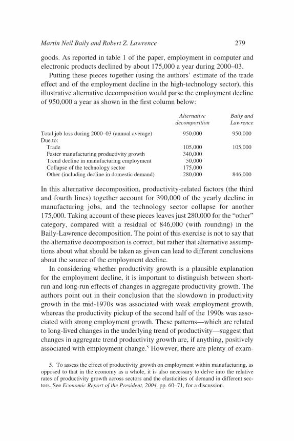
goods. As reported in table 1 of the paper, employment in computer andelectronic products declined by about 175,000 a year during 2000–03.

Putting these pieces together (using the authors’ estimate of the tradeeffect and of the employment decline in the high-technology sector), thisillustrative alternative decomposition would parse the employment declineof 950,000 a year as shown in the first column below:

Alternative Baily anddecomposition Lawrence

Total job loss during 2000–03 (annual average) 950,000 950,000Due to:

Trade 105,000 105,000Faster manufacturing productivity growth 340,000Trend decline in manufacturing employment 50,000Collapse of the technology sector 175,000Other (including decline in domestic demand) 280,000 846,000

In this alternative decomposition, productivity-related factors (the thirdand fourth lines) together account for 390,000 of the yearly decline inmanufacturing jobs, and the technology sector collapse for another175,000. Taking account of these pieces leaves just 280,000 for the “other”category, compared with a residual of 846,000 (with rounding) in theBaily-Lawrence decomposition. The point of this exercise is not to say thatthe alternative decomposition is correct, but rather that alternative assump-tions about what should be taken as given can lead to different conclusionsabout the source of the employment decline.

In considering whether productivity growth is a plausible explanationfor the employment decline, it is important to distinguish between short-run and long-run effects of changes in aggregate productivity growth. Theauthors point out in their conclusion that the slowdown in productivitygrowth in the mid-1970s was associated with weak employment growth,whereas the productivity pickup of the second half of the 1990s was asso-ciated with strong employment growth. These patterns—which are relatedto long-lived changes in the underlying trend of productivity—suggest thatchanges in aggregate trend productivity growth are, if anything, positivelyassociated with employment change.5 However, there are plenty of exam-


5. To assess the effect of productivity growth on employment within manufacturing, asopposed to that in the economy as a whole, it is also necessary to delve into the relativerates of productivity growth across sectors and the elasticities of demand in different sec-tors. See Economic Report of the President, 2004, pp. 60–71, for a discussion.


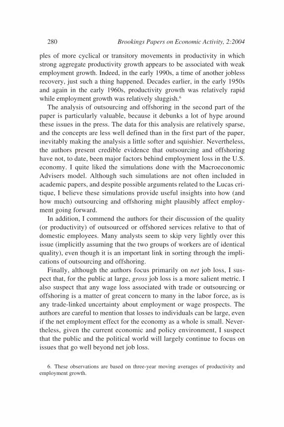
ples of more cyclical or transitory movements in productivity in whichstrong aggregate productivity growth appears to be associated with weakemployment growth. Indeed, in the early 1990s, a time of another joblessrecovery, just such a thing happened. Decades earlier, in the early 1950sand again in the early 1960s, productivity growth was relatively rapidwhile employment growth was relatively sluggish.6

The analysis of outsourcing and offshoring in the second part of thepaper is particularly valuable, because it debunks a lot of hype aroundthese issues in the press. The data for this analysis are relatively sparse,and the concepts are less well defined than in the first part of the paper,inevitably making the analysis a little softer and squishier. Nevertheless,the authors present credible evidence that outsourcing and offshoringhave not, to date, been major factors behind employment loss in the U.S.economy. I quite liked the simulations done with the MacroeconomicAdvisers model. Although such simulations are not often included inacademic papers, and despite possible arguments related to the Lucas cri-tique, I believe these simulations provide useful insights into how (andhow much) outsourcing and offshoring might plausibly affect employ-ment going forward.

In addition, I commend the authors for their discussion of the quality(or productivity) of outsourced or offshored services relative to that ofdomestic employees. Many analysts seem to skip very lightly over thisissue (implicitly assuming that the two groups of workers are of identicalquality), even though it is an important link in sorting through the impli-cations of outsourcing and offshoring.

Finally, although the authors focus primarily on net job loss, I sus-pect that, for the public at large, gross job loss is a more salient metric. Ialso suspect that any wage loss associated with trade or outsourcing oroffshoring is a matter of great concern to many in the labor force, as isany trade-linked uncertainty about employment or wage prospects. Theauthors are careful to mention that losses to individuals can be large, evenif the net employment effect for the economy as a whole is small. Never-theless, given the current economic and policy environment, I suspectthat the public and the political world will largely continue to focus onissues that go well beyond net job loss.


6. These observations are based on three-year moving averages of productivity andemployment growth.


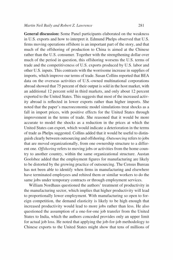
General discussion: Some Panel participants elaborated on the weaknessin U.S. exports and how to interpret it. Edmund Phelps observed that U.S.firms moving operations offshore is an important part of the story, and thatmuch of the offshoring of production to China is aimed at the Chineserather than the U.S. consumer. Together with the strengthening dollar overmuch of the period in question, this offshoring worsens the U.S. terms oftrade and the competitiveness of U.S. exports produced by U.S. labor andother U.S. inputs. This contrasts with the worrisome increase in supplies ofimports, which improve our terms of trade. Susan Collins reported that BEAdata on the overseas activities of U.S.-owned multinational corporationsabroad showed that 75 percent of their output is sold in the host market, withan additional 12 percent sold in third markets, and only about 12 percentexported to the United States. This suggests that most of the increased activ-ity abroad is reflected in lower exports rather than higher imports. Shenoted that the paper’s macroeconomic model simulations treat shocks as afall in import prices, with positive effects for the United States throughimprovement in the terms of trade. She reasoned that it would be moreaccurate to model the shocks as a reduction in the prices at which theUnited States can export, which would indicate a deterioration in the termsof trade as Phelps suggested. Collins added that it would be useful to distin-guish clearly between outsourcing and offshoring. Outsourcing refers to jobsthat are moved organizationally, from one ownership structure to a differ-ent one. Offshoring refers to moving jobs or activities from the home coun-try to another country, within the same organizational structure. AustanGoolsbee added that the employment figures for manufacturing are likelyto be distorted by the growing practice of outsourcing. The Census Bureauhas not been able to identify when firms in manufacturing and elsewherehave terminated employees and rehired them or similar workers to do thesame jobs under temporary contracts or through employment services.

William Nordhaus questioned the authors’ treatment of productivity inthe manufacturing sector, which implies that higher productivity will leadto proportionally lower employment. With manufacturing so open to for-eign competition, the demand elasticity is likely to be high enough thatincreased productivity would lead to more jobs rather than less. He alsoquestioned the assumption of a one-for-one job transfer from the UnitedStates to India, which the authors conceded provides only an upper limitfor actual job loss. He noted that applying the job-for-job methodology toChinese exports to the United States might show that tens of millions of



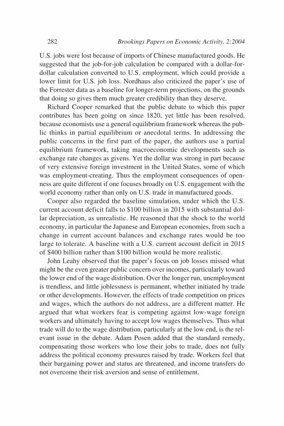
U.S. jobs were lost because of imports of Chinese manufactured goods. Hesuggested that the job-for-job calculation be compared with a dollar-for-dollar calculation converted to U.S. employment, which could provide alower limit for U.S. job loss. Nordhaus also criticized the paper’s use ofthe Forrester data as a baseline for longer-term projections, on the groundsthat doing so gives them much greater credibility than they deserve.

Richard Cooper remarked that the public debate to which this papercontributes has been going on since 1820, yet little has been resolved,because economists use a general equilibrium framework whereas the pub-lic thinks in partial equilibrium or anecdotal terms. In addressing thepublic concerns in the first part of the paper, the authors use a partialequilibrium framework, taking macroeconomic developments such asexchange rate changes as givens. Yet the dollar was strong in part becauseof very extensive foreign investment in the United States, some of whichwas employment-creating. Thus the employment consequences of open-ness are quite different if one focuses broadly on U.S. engagement with theworld economy rather than only on U.S. trade in manufactured goods.

Cooper also regarded the baseline simulation, under which the U.S.current account deficit falls to $100 billion in 2015 with substantial dol-lar depreciation, as unrealistic. He reasoned that the shock to the worldeconomy, in particular the Japanese and European economies, from such achange in current account balances and exchange rates would be toolarge to tolerate. A baseline with a U.S. current account deficit in 2015of $400 billion rather than $100 billion would be more realistic.

John Leahy observed that the paper’s focus on job losses missed whatmight be the even greater public concern over incomes, particularly towardthe lower end of the wage distribution. Over the longer run, unemploymentis trendless, and little joblessness is permanent, whether initiated by tradeor other developments. However, the effects of trade competition on pricesand wages, which the authors do not address, are a different matter. Heargued that what workers fear is competing against low-wage foreignworkers and ultimately having to accept low wages themselves. Thus whattrade will do to the wage distribution, particularly at the low end, is the rel-evant issue in the debate. Adam Posen added that the standard remedy,compensating those workers who lose their jobs to trade, does not fullyaddress the political economy pressures raised by trade. Workers feel thattheir bargaining power and status are threatened, and income transfers donot overcome their risk aversion and sense of entitlement.



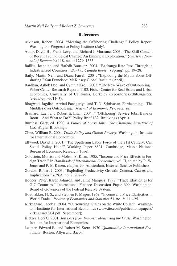
References

Atkinson, Robert. 2004. “Meeting the Offshoring Challenge.” Policy Report.Washington: Progressive Policy Institute (July).

Autor, David H., Frank Levy, and Richard J. Murnane. 2003. “The Skill Contentof Recent Technological Change: An Empirical Exploration.” Quarterly Jour-nal of Economics 118, no. 4: 1279–1333.

Bailliu, Jeannine, and Hafedh Bouakez. 2004. “Exchange Rate Pass-Through inIndustrialized Countries.” Bank of Canada Review (Spring), pp. 19–28.

Baily, Martin Neil, and Diana Farrell. 2004. “Exploding the Myths about Off-shoring.” San Francisco: McKinsey Global Institute (April).

Bardhan, Ashok Deo, and Cynthia Kroll. 2003. “The New Wave of Outsourcing.”Fisher Center Research Reports 1103. Fisher Center for Real Estate and UrbanEconomics, University of California, Berkeley (repositories.cdlib.org/iber/fcreue/reports/1103).

Bhagwati, Jagdish, Arvind Panagariya, and T. N. Srinivasan. Forthcoming. “TheMuddles over Outsourcing.” Journal of Economic Perspectives.

Brainard, Lael, and Robert E. Litan. 2004. “ ‘Offshoring’ Service Jobs: Bane orBoon—And What to Do?” Policy Brief 132. Brookings (April).

Burtless, Gary, ed. 1990. A Future of Lousy Jobs? The Changing Structure ofU.S. Wages. Brookings.

Cline, William R. 2004. Trade Policy and Global Poverty. Washington: Institutefor International Economics.

Ellwood, David T. 2001. “The Sputtering Labor Force of the 21st Century: CanSocial Policy Help?” Working Paper 8321. Cambridge, Mass.: NationalBureau of Economic Research (June).

Goldstein, Morris, and Mohsin S. Khan. 1985. “Income and Price Effects in For-eign Trade.” In Handbook of International Economics, vol. II, edited by R. W.Jones and P. B. Kenen, chapter 20. Amsterdam: Elsevier Science Publishers.

Gordon, Robert J. 2003. “Exploding Productivity Growth: Context, Causes andImplications.” BPEA, no. 2: 207–79.

Hooper, Peter, Karen Johnson, and Jaime Marquez. 1998. “Trade Elasticities forG-7 Countries.” International Finance Discussion Paper 609. Washington:Board of Governors of the Federal Reserve System.

Houthakker, H. S., and Stephen P. Magee. 1969. “Income and Price Elasticities inWorld Trade.” Review of Economics and Statistics 51, no. 2: 111–25.

Kirkegaard, Jacob F. 2004. “Outsourcing: Stains on the White Collar?” Washing-ton: Institute for International Economics (www.iie.com/publications/papers/kirkegaard0204.pdf [September]).

Kletzer, Lori G. 2001. Job Loss from Imports: Measuring the Costs. Washington:Institute for International Economics.

Leamer, Edward E., and Robert M. Stern. 1970. Quantitative International Eco-nomics. Boston: Allyn and Bacon.



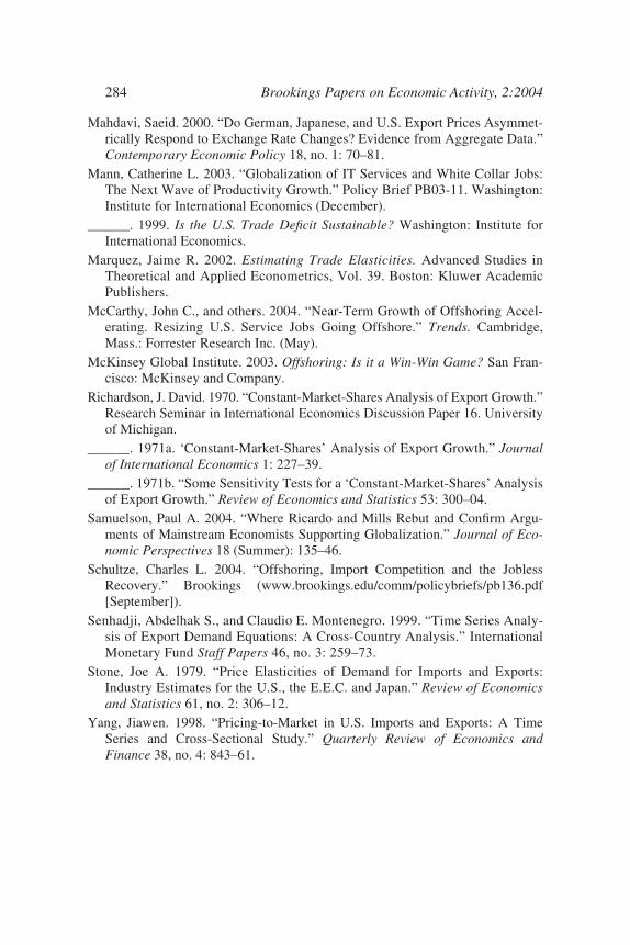
Mahdavi, Saeid. 2000. “Do German, Japanese, and U.S. Export Prices Asymmet-rically Respond to Exchange Rate Changes? Evidence from Aggregate Data.”Contemporary Economic Policy 18, no. 1: 70–81.

Mann, Catherine L. 2003. “Globalization of IT Services and White Collar Jobs:The Next Wave of Productivity Growth.” Policy Brief PB03-11. Washington:Institute for International Economics (December).

______. 1999. Is the U.S. Trade Deficit Sustainable? Washington: Institute forInternational Economics.

Marquez, Jaime R. 2002. Estimating Trade Elasticities. Advanced Studies inTheoretical and Applied Econometrics, Vol. 39. Boston: Kluwer AcademicPublishers.

McCarthy, John C., and others. 2004. “Near-Term Growth of Offshoring Accel-erating. Resizing U.S. Service Jobs Going Offshore.” Trends. Cambridge,Mass.: Forrester Research Inc. (May).

McKinsey Global Institute. 2003. Offshoring: Is it a Win-Win Game? San Fran-cisco: McKinsey and Company.

Richardson, J. David. 1970. “Constant-Market-Shares Analysis of Export Growth.”Research Seminar in International Economics Discussion Paper 16. Universityof Michigan.

______. 1971a. ‘Constant-Market-Shares’ Analysis of Export Growth.” Journalof International Economics 1: 227–39.

______. 1971b. “Some Sensitivity Tests for a ‘Constant-Market-Shares’ Analysisof Export Growth.” Review of Economics and Statistics 53: 300–04.

Samuelson, Paul A. 2004. “Where Ricardo and Mills Rebut and Confirm Argu-ments of Mainstream Economists Supporting Globalization.” Journal of Eco-nomic Perspectives 18 (Summer): 135–46.

Schultze, Charles L. 2004. “Offshoring, Import Competition and the JoblessRecovery.” Brookings (www.brookings.edu/comm/policybriefs/pb136.pdf[September]).

Senhadji, Abdelhak S., and Claudio E. Montenegro. 1999. “Time Series Analy-sis of Export Demand Equations: A Cross-Country Analysis.” InternationalMonetary Fund Staff Papers 46, no. 3: 259–73.

Stone, Joe A. 1979. “Price Elasticities of Demand for Imports and Exports:Industry Estimates for the U.S., the E.E.C. and Japan.” Review of Economicsand Statistics 61, no. 2: 306–12.

Yang, Jiawen. 1998. “Pricing-to-Market in U.S. Imports and Exports: A TimeSeries and Cross-Sectional Study.” Quarterly Review of Economics andFinance 38, no. 4: 843–61.



What Happened to the Great U.S. Job Machine? The Role of ...€¦ · argument goes, U.S. workers...

Documents

Transcript of What Happened to the Great U.S. Job Machine? The Role of ...€¦ · argument goes, U.S. workers...