http://econ.geog.uu.nl/peeg/peeg.html

Papers in Evolutionary Economic Geography

#18.13

What Drives the Geography of Jobs in the US? Unpacking Relatedness

Teresa Farinha Fernandes and Pierre-Alexandre Balland and Andrea Morrison and Ron Boschma

1

WHAT DRIVES THE GEOGRAPHY OF JOBS IN THE US? UNPACKING RELATEDNESS

Teresa Farinha Fernandes*#, Pierre-Alexandre Balland*, Andrea Morrison*^

and Ron Boschma*$

*Department of Human Geography and Planning, Utrecht University # IN+ Center for Innovation, Technology and Policy Research, Lisboa University

$ UiS Business School, University of Stavanger ^Icrios-Bocconi University

12 March 2018

ABSTRACT

There is ample evidence of regions diversifying in new occupations that are related to pre-existing activities in the region. However, it is still poorly understood through which mechanisms related diversification operates. To unpack relatedness, we distinguish between three mechanisms: complementarity (interdependent tasks), similarity (sharing similar skills) and local synergy (based on pure co-location). We propose a measure for each of these relatedness dimensions and assess their impact on the evolution of the occupational structure of 389 US Metropolitan Statistical Areas (MSA) for the period 2005-2016. Our findings show that new jobs appearing in MSA’s are related to existing ones, while those more likely to disappear are more unrelated to a city’s jobs’ portfolio. We found that all three relatedness dimensions matter, but local synergy shows the largest impact on entry and exit of jobs in US cities.

Keywords: evolutionary economic geography, regional capabilities, jobs, skills, relatedness, similarity, complementarity, local synergy, US cities

JEL: J24, O18, R10

1 INTRODUCTION

The 2008 crisis has led to unprecedented job losses and the destruction of human capital in many regions worldwide. On top of that, technological change, automation, and offshoring of

2

jobs are leaving their marks (Autor 2010; Rodriguez and Jayadev 2010; Moretti 2012; Mehta 2014). Though such shocks and global trends affect all regional economies, they tend to do so in varying degrees (Shutters et al. 2015). This has initiated a recent interest of scholars to study systematically the evolution of occupational structures in regions over time.

Muneepeerakul et al. (2013) was the first study assessing how relatedness affects entry and exit of occupations in US metropolitan regions (see also Brachert 2016; Shutter et al. 2016). These studies follow a recent body of literature on regional diversification that shows that regions tend to diversify into new industries (e.g. Neffke et al. 2011; Boschma et al. 2013; Essletzbichler 2015; He and Rigby 2015) or new technologies (Kogler et al. 2013; Rigby 2015) that are closely related to their pre-existing capabilities. What these studies on regional diversification have not unraveled so far are the mechanisms through which industries, technologies or occupations may be related. In fact, there is still little understanding of the sources of relatedness that impact on regional diversification (Tanner 2014; Boschma 2017).

The main objective of this paper is to unpack the mechanisms through which the entry and exit of jobs in cities take place. While previous papers looked at the effect of geographical density only, we argue that co-location of jobs tells little about the forces that make jobs co-occur in the same city: new local jobs may be related to local jobs because they share similar skills, provide complementary tasks, or both, or because they benefit from each other’s co-location. We make a distinction between three mechanisms: (1) occupations can be related because they incorporate a similar set of skills of high relevance for each job; (2) occupations may be complementary in the process of producing a good or service; and (3) occupations may jointly benefit from synergies in cities. There is no study yet that has investigated the importance of each of these three mechanisms in the evolution of the geography of jobs.

We use a network approach to unpack the relatedness concept into three dimensions and develop a measure for each of them. We test the impact of each relatedness dimension on the dynamics of the occupational structure of 389 Metropolitan Statistical Areas in the US from 2005 to 2016, more specifically, on the probability of occupations entering and exiting the employment structure of cities. Our paper confirms the results found in other studies that cities enter new jobs related to ones already existing in that cities, and exit jobs unrelated to their jobs portfolio. Moreover, we found that all three relatedness dimensions have a significant effect but they seem to prevent exit of jobs in cities more than promoting entry of jobs in cities. Local synergy density shows the largest effect on both entry and exit of jobs in cities.

The structure of the paper is as follows. In Section 2, we present the concept of relatedness as developed in Evolutionary Economic Geography, and we explain how we unpack relatedness into three dimensions. Section 3 presents the data, our measures for each relatedness dimension, and the network representation of the occupational structure. Section 4 presents the study on how job relatedness, in its different dimensions, has influenced the entry and exit of occupational specializations in US cities. Section 5 discusses the results and concludes.

2 REGIONAL DIVERSIFICATION IN JOBS: THREE MECHANISMS

3

In Evolutionary Economic Geography, history is key to understand the economic evolution of regions (Boschma and Frenken 2006; Martin and Sunley 2006). Past structures set opportunities but also boundaries to future development. A large body of empirical studies shows that diversification occurs in regions mainly by making use of and recombining pre-existing regional capabilities: in other words, it is subject to path-dependency (Boschma 2017). Moreover, regions localized in the dense parts of the ‘product space’ (i.e. having many products related to each other) have also more diversification options and higher economic growth rates (Frenken et al. 2007; Hidalgo et al. 2007; Hausmann and Hidalgo 2010).

These studies tend to look at diversification in terms of new products (Hidalgo et al. 2007), new industries (Neffke et al. 2011) or new technologies (e.g. Kogler et al. 2013; Rigby 2015, Petralia et al. 2017; Balland et al., 2018). However, industry, product, and technology classifications capture some but not all capabilities in regions (Markusen 2004; Moretti and Kline 2014). This point was made by Thompson and Thompson (1985, 1987) who made a strong claim in favour of an occupational functional approach to understand the changing spatial division of labour in which advanced regions focus on high value-added activities and jobs (design, marketing, R&D) while off-shoring labour-intensive (and low-skilled) jobs to places where labour costs are comparatively low (Gereffi and Korzeniewicz 1994; Markusen et al. 2001; Markusen and Schrock 2006; Barbour and Markusen 2007; Renski et al. 2007). This growing separation of functions within the same industry implies that regions with similar industrial specialisations can reflect very different underlying capabilities in terms of knowledge and skills (Markusen et al. 2008). Technology classifications do not cover all capabilities in regions either because they tend to capture scientific and technical skills. Shifting away from industries and technologies to jobs reveal what regions do with their skills, as opposed to what regions make as the outcome of their activity (Thompson and Thompson 1985; Feser 2003). This change of perspective is important as growth opportunities in knowledge-based economies are considered to depend on the accumulation of human rather than physical capital (Moretti 2012). And last but not least, an occupational approach can cover better service industries than the industry/technology approach.

Muneepeerakul et al. (2013), Brachert (2016) and Shutter et al. (2016) were the first to acknowledge the relevance of the occupational structure to analyse regional evolution. These studies provide a network representation of the structure of interdependent job classes in US cities, called occupational space. They show that co-located occupational specializations can interact positively or negatively with each other; and that the balance between these interactions determines productivity, wealth, and possible development paths of urban economies. Hasan et al. (2015) found that interdependencies between jobs (either as task overlap or task coordination) tend to protect jobs. On the other hand, regarding the whole job structure, they found that interdependence (ties between jobs) makes a job vulnerable to the exit of other jobs in that job’s cluster, decreasing its survival chance.

However, these studies on job diversification in cities have not looked at the types of mechanisms through which related diversification unfolds. This means we have to unpack the broad notion of relatedness, as advocated by some scholars (Breschi et al. 2003; Tanner 2014;

4

Boschma 2017). Inspired by Duranton and Puga (2003), we distinguish between three mechanisms or channels through which agglomeration externalities may be exploited, and we make an explicit connection to job dynamics.

The first mechanism refers to similarity of skills between jobs. This applies when a certain set of skills can be used to perform more than one type of task or job activity: job classes that have those skills are similar (but not identical) and substitutable to a considerable degree. This has a close resemblance with the notion of skill-relatedness introduced by Neffke and Henning (2013). The second mechanism refers to complementarity of skills between jobs. Here, skills in different job classes are required to produce a certain good or service within a value chain, like a doctor and a nurse in a hospital provide complementary skills to cure illnesses. In modern societies, as products/services complexity increases, the amount of interdependent tasks increases within each value chain. We will capture this skill complementarity by looking at the co-occurrence of job classes in economic activities. The third mechanism is associated with local synergy effects between different jobs when the co-location of two jobs (e.g. a business man and a taxi driver) benefit each other, while not being similar or complementary in skills with one another. These local synergies may arise due to common natural endowments, demand-driven interdependencies of jobs, or amenities (Florida 2002; Moretti 2012). This latter dimension also covers local multipliers in which high-skilled jobs provide benefits for low-skilled jobs (Moretti 2013; Moretti and Kline 2014). We will capture local synergy by identifying the geographical co-occurrence of job classes, after having it filtered from the other two dimensions.

There is no study yet that has investigated the importance of each of these three mechanisms in the evolution of the geography of jobs. We examine which of the mechanisms can explain best the entry of new jobs and the exit of existing jobs in 389 US cities from 2005 to 2016.

3 OCCUPATIONAL DATA AND NETWORK ANALYSIS 3.1 OCCUPATIONAL DATA

The main source is employment data provided by the Bureau of Labor Statistics of the U.S. Department of Labor (BLS)1. It contains several workers statistics, such as total employment and mean hourly wage by job class (approximately 800 categories at the 6-digit level) by industry (NAICS) and by U.S. Metropolitan Statistical Areas (MSA). The Standard Occupational Classification (SOC) System groups similar jobs into job classes (OCC) based on the work performed, skills, education, training, and credentials required to carry out specific work tasks. Some OCC are found in just one or two industries, others in a large number of industries. NAICS is a production-oriented classification that groups establishments into industries based on their prime activity. MSAs represent unified labour markets (Muneepeerakul et al., 2013). Each MSA contains a core urban area of at least 50.000 population in one or more core counties, including adjacent counties with a high

1 publicly available at http://www.bls.gov/oes

5

degree of social and economic integration with the urban core. MSAs account for nearly 85% of U.S. population and 90% of U.S. economic output (US Census Bureau, 2015).

To account for classification schemes revisions and assure a comparable multi-year analysis, we use data from 2005 to 2016 and exclude from our analysis the MSAs (eight MSA and five NECTA) and the OCCs that came into existence after 2005, and the “All Other” type of OCC which is not available in the O*NET data2. After cleaning data, we end up with statistics on number of people employed in each year-OCC-MSA (12 years, 733 OCC, and 389 MSA).

After that, we cross the BLS employment data with occupational content classification from the Occupational Information Network (O*NET). O*NET provides a detailed classification of occupational contents – occupational requirements and worker attributes for each job class3. O*NET attributes to each job class the correspondent workers’ capabilities, according to the O*NET classification schemes. After testing their typology and employment data distributions, we chose the Intermediate Work Activities (IWA)4 classification scheme that represents all skill specifications needed to perform each job class5, and is, therefore, better suited to compute our measure of job similarity. The result is a dataset with job requirement weight for each OCC-Skills (same 733 OCC, 332 Work Activities).

Because many unified product value chains bring together different NAICS classifications, we cross the BLS employment data with an industry classification defined and made available by BLS, the Industry Sectoring Plan6. This industry classification groups together the narrowly defined U.S. industry codes (NAICS) that are related in terms of inter-industry linkages (input-output measures) into industry sectors, or more simply referred as clusters. In other words, we aggregate the BLS employment-OCC-NAICS data into an employment-OCC-cluster dataset for the last year of the period under consideration (same 733 OCC, 179 industry clusters, for the year 2016)7. The result is an industry cluster’s labour demand dataset, from which we compute our job complementarity measure.

2"All Other" titles represent job classes with a wide range of characteristics, which do not fit into one of the detailed O*NET-SOC occupations. 3 publicly available at https://www.onetonline.org 4 O*NET provides classification schemes for Work Activities at three levels of aggregation (41 Generalized Work Activities; 332 Intermediate Work Activities; and finally, 2070 Detailed Work Activities). Intermediate Work Activities is the level of aggregation that provides us better network analysis conditions (enough categories, and that are not too common and not too rare across job classes) 5 Here we refer to skills in its broad sense, equivalent to the concept of regional capabilities, commonly used in the evolutionary economic geography literature. It corresponds not to O*NET classification schemes for skills (which refers to a much stricter sense of skills), but to O*NET definition of workers’ competencies (it includes classification schemes for skills in the stricter sense, knowledge, abilities, experience and training, etc.). 6 BLS aggregates NAICS (4 digit level) into the industry sectors, further used in BLS’s employment projections (https://www.bls.gov/emp/ep_data_input_output_matrix.htm)7Duetoclassificationscorrespondenceconstrains,weexcludethe“Privatehouseholds”sector(notavailableinBLSemploymentdata)andfurtherpulltogetherafewindustrysectors,endingupwith179sectorsinsteadof186.Morespecifically,weaggregateintoonethe“Cropproduction”,“Animalproductionandaquaculture”,

6

After cleaning and merging data, we compute the geographical measure of relatedness (co-location-based measure), and our measures for complementarity and similarity dimensions of relatedness. We obtain a bipartite dataframe with three variables of relatedness for each possible pair of job classes in each year. We use this data in the network analysis and further transform it into a new dataset to be used in the regression analysis. For ease of interpretation, we will use the terms “job class”, “city”, “industry”, and “skills” when referring to OCC, MSAs, Industry Sectoring Plan categories, and Work Activities, respectively.

3.2 UNPACKING RELATEDNESS

In line with the network-based framework of Hidalgo et al (2007) and Muneepeerakul et al. (2013), we build a network of job classes and relatedness between them – the Job Space – to represent the U.S. labour market structure. The Job Space will have three types of links based on three measures of relatedness: a geographical, a complementarity and a similarity measure. From those three measures of relatedness, we will deduce the fourth one for the local synergies dimension of relatedness – the pairs of job classes that are poorly complementary, poorly similar, but most frequently co-located, due to local synergies.

- Geographical relatedness of jobs

First, we identify job classes in which U.S. cities specialize in. We use the location quotient (LQ) of job class j in city c, based on the number of employees (x) engaged in job class j, in city c, in relation with the total number of employees engaged in job class j in the country:

!"#,% =

'#,%'#,%%

'#,%#

'#,%%#

A LQ higher than one means that the proportion of the labour force engaged in that job class is “overrepresented” in that city. As a result, we get a binary jobs-cities matrix (N×M matrix). Then, we compute the geographical measure of relatedness between each pair of job classes, based on their co-occurrences as specializations in cities, for each year during the 2005-2013 period. More concretely, we use a conditional-probability-based measure developed by Van Eck & Waltman (2009) and reformulated by Steijn (forthcoming). This results in a symmetric N×N job classes matrix, in which each cell (i, j) contains the geographical measure of relatedness (GeoRel) between job class i and job class j, i.e., the probability of a city c being specialized in job class i given that it is also specialized in job class j, as follows:

“Forestry”(including“SupportActivitiesforForestry”),and“Fishing,huntingandtrapping”.Wealsoaggregateintoonethegovernmentalsectors(whichcorrespondstothe2digitsNAICS92–PublicAdministration).

7

GeoRel (()*,S), -*, .) = ()* / (m * ((-)/.) * -*/ (. – -)) + (-*/.) * (-)/(. – -*)))

where Cij, Si, and Sj are, respectively, the number of co-occurrences of i and j, the number of occurrences of job class i and the number of occurrences of job class j, as occupational specializations in cities. . is the sum of all cities occupational specializations, and m is the total number of co-occurrences. The geographical measure of relatedness indicates the probability of two job classes being together in the same city. GeoRel is lower bounded by zero (job classes i and j are never together as specializations in same city) but not upper bounded. A GeoRel higher than 1 means that two job classes co-locate in the same city more often than by chance.

Although commonly used as an outcome-based measure of relatedness, co-location of job classes does not inform us about the type(s) of relatedness between two jobs. In order to empirically unpack the dimensions of relatedness for each pair of job classes, we create other two measures of relatedness: jobs similarity and jobs complementarity.

- Jobs similarity

Based on BLS job classes and O*NET’s Work Activities classification scheme, we compute jobs similarity as the frequency of co-occurrences of jobs classes in work activities classes. More specifically, in line with Hasan et al (2015), we first construct a 1×W vector for each job class, with W being the number of O*NET IWA categories, and join them to form a binary jobs-IWA matrix (N×W matrix). Then, we apply conditional probabilities for computing jobs similarity measure of relatedness (equivalent to the GeoRel equation, the jobs co-location measure, but based on the jobs-IWA matrix instead). In result, we get a symmetric N×N job classes matrix in which each cell (i, j) contains the skills similarity between job classes i and j. In other words, skills similarity represents, therefore, job classes’ co-occurrences in IWA as the main occupational destination of such skills (e.g., Work Activity w is a highly required skill, more than average in regional labour markets, for both job class a and b).

- Jobs complementarity

Based on industry clusters’ labour demand, we compute complementarity by looking at which pairs of job classes are jointly required in the same value chain(s). We determine how often two job classes co-occur in the same industry cluster. We first compute each industry cluster’s LQ in each job class, i.e., each cluster employment shares in each job class, compared to the average employment shares of all clusters (same LQ equation we used for jobs co-location measure, but based on the jobs-cluster matrix). Then, we apply conditional probabilities for measuring jobs complementarity (equivalent to GeoRel equation but based

8

on the jobs-cluster matrix). So, we construct a symmetric N×N job classes matrix in which each cell (i, j) contains the jobs complementarity index between job classes i and j.

- Jobs local synergies

From the three measures of geographical relatedness, complementarity and similarity, we can derive the local synergies dimension of relatedness. Pure geographical relatedness confounds the different forces that make jobs co-occur in the same city. Indeed, jobs may co-locate for reasons of complementarity or similarity, so we cannot tell for sure if local synergies do operate or not. However, local synergies are notoriously difficult to identify. They refer to strong agglomerative forces, but not of the complementarity and the similarity kind. Because some pairs of complementary and/or similar job classes may also have a tendency to co-locate, we need to control for that. We argue that if two job classes have high geographical relatedness but low skills similarity and low industry complementarity, we assume these two job classes show local synergies. So, we deduce the presence of local synergies by identifying pairs of job classes that are most probable to co-locate in cities but do neither show a high degree of jobs complementary nor high jobs similarity.

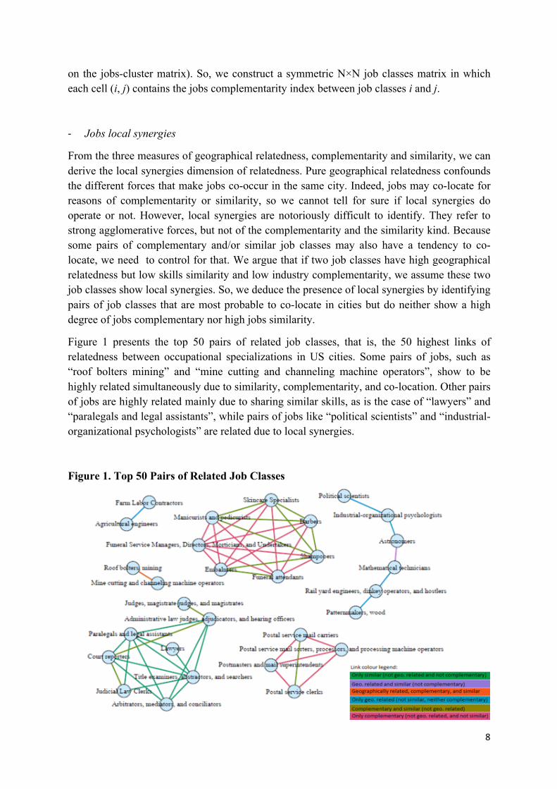
Figure 1 presents the top 50 pairs of related job classes, that is, the 50 highest links of relatedness between occupational specializations in US cities. Some pairs of jobs, such as “roof bolters mining” and “mine cutting and channeling machine operators”, show to be highly related simultaneously due to similarity, complementarity, and co-location. Other pairs of jobs are highly related mainly due to sharing similar skills, as is the case of “lawyers” and “paralegals and legal assistants”, while pairs of jobs like “political scientists” and “industrial-organizational psychologists” are related due to local synergies.

Figure 1. Top 50 Pairs of Related Job Classes

9

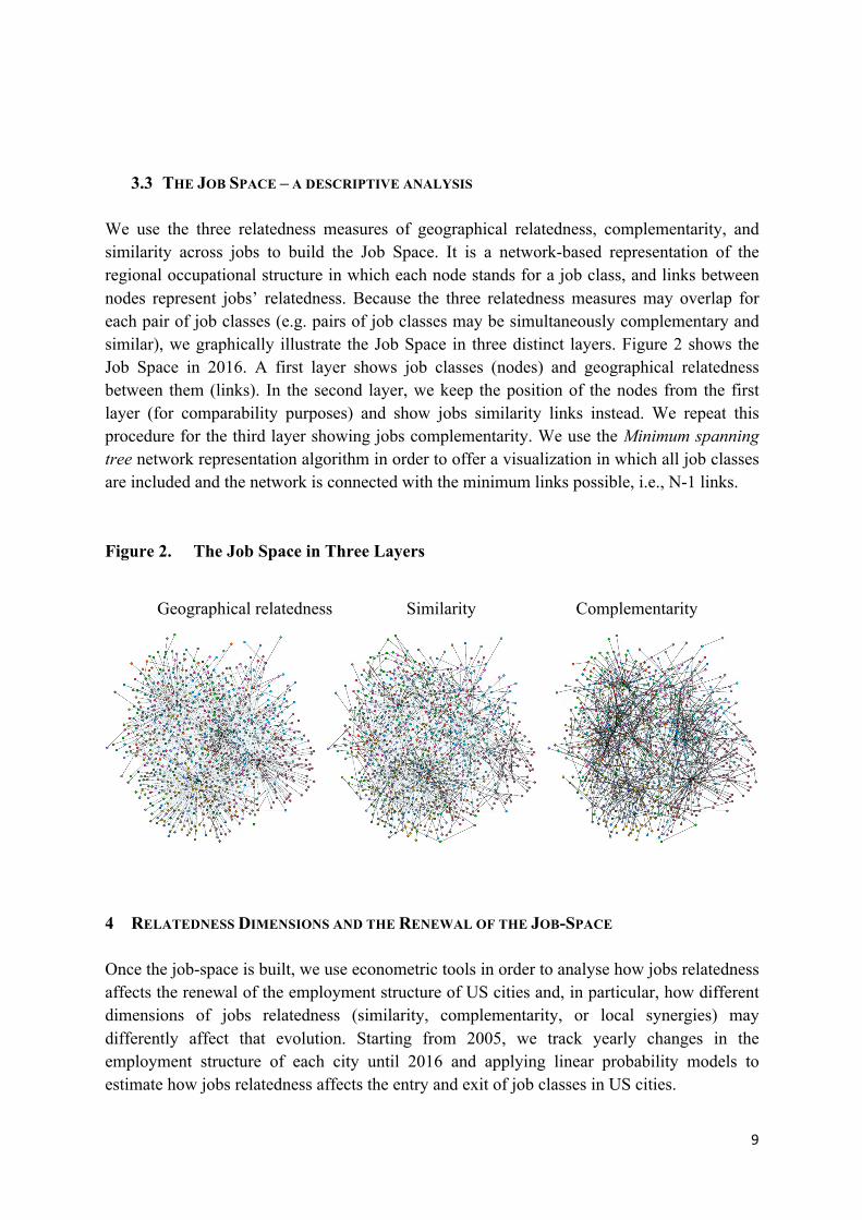
3.3 THE JOB SPACE – A DESCRIPTIVE ANALYSIS

We use the three relatedness measures of geographical relatedness, complementarity, and similarity across jobs to build the Job Space. It is a network-based representation of the regional occupational structure in which each node stands for a job class, and links between nodes represent jobs’ relatedness. Because the three relatedness measures may overlap for each pair of job classes (e.g. pairs of job classes may be simultaneously complementary and similar), we graphically illustrate the Job Space in three distinct layers. Figure 2 shows the Job Space in 2016. A first layer shows job classes (nodes) and geographical relatedness between them (links). In the second layer, we keep the position of the nodes from the first layer (for comparability purposes) and show jobs similarity links instead. We repeat this procedure for the third layer showing jobs complementarity. We use the Minimum spanning tree network representation algorithm in order to offer a visualization in which all job classes are included and the network is connected with the minimum links possible, i.e., N-1 links.

Figure 2. The Job Space in Three Layers Geographical relatedness Similarity Complementarity

4 RELATEDNESS DIMENSIONS AND THE RENEWAL OF THE JOB-SPACE

Once the job-space is built, we use econometric tools in order to analyse how jobs relatedness affects the renewal of the employment structure of US cities and, in particular, how different dimensions of jobs relatedness (similarity, complementarity, or local synergies) may differently affect that evolution. Starting from 2005, we track yearly changes in the employment structure of each city until 2016 and applying linear probability models to estimate how jobs relatedness affects the entry and exit of job classes in US cities.

10

4.1 VARIABLES AND DESCRIPTIVES

We first construct two dummy variables, Entry and Exit. Entry is conventionally computed as equal to one if a job class did not belong to the occupational specialization portfolio of city c in time t-1, and enters in time t. And Exit is equal to one if a job class did belong to the occupational specialization portfolio of city c in time t-1, but exits in time t:

/0123#,4,5 = 1, if!"#,4,5 > 1:0;!"#,4,5<= ≤ 1

/')1#,4,5 = 1, if!"#,4,5 ≤ 1:0;!"#,4,5<= > 1

LQ ranks cities level of specialization in relation to the average level of specialization of all regions in a year. This means that the position in the ranking of a city may vary from one year to another, not due to changes in that city’s level of specialization but to changes in other cities’ level of specialization that affect the average level of specialization of an economy. So, a job class could change from being a city specialization t-1 but not anymore in t, just because the ranking of specialization of that job class increased overall in the average economy, not because the share of employees in that city decreased. To exclude such “false” changes in computing Entry and Exit, we made a slight adjustment to the LQ in t 8. We track the evolution of an occupational specialization in the city in relation to the pre-existing structure of the city, from t-1 to t, independent of the evolution of the economy’s average specialization level, which we fix at t-1 when computing LQ in t, as follows:

/0123#,4,5 = 1, if!"#,4,5,5<= > 1:0;!"#,4,5<=,5<= ≤ 1

/')1#,4,5 = 1, if!"#,4,5,5<= ≤ 1:0;!"#,4,5<=,5<= > 1

which translates into:

/0123#,4,5 = 1, if

'#,4'#,44

1

'#,4#

'#,44#1 − 1

> 1:0;

'#,4'#,44

1 − 1

'#,4#

'#,44#1 − 1

≤ 1

8Forrobustnesspurposes,wealsocomputedEntryandExitinitstraditionalformandrunthesamemodelsinouranalysis.Theeconometricresultsareverysimilar,withcoefficientschangingonlyslightlyandkeepingitsstatisticalandeconomicsignificance.

11

/')1#,4,5 = 1, if

'#,4'#,44

1

'#,4#

'#,44#1 − 1

≤ 1:0;

'#,4'#,44

1 − 1

'#,4#

'#,44#1 − 1

> 1

We must account for other variables that may influence Entry and Exit of cities’ occupational specializations. In our econometric analysis, we use three-way-fixed effects models, with fixed effects for job classes (@%), cities (A#), and years (B5), accounting for unobservable and invariant specific economic context. In addition, we use six control variables. Because a bigger and/or more diversified city is more prone to attract new jobs, we compute, for each city in each year, its total employment (log) (City total employment) and its number of occupational specializations (City diversity). To account for short-term employment growth (especially for years during the crisis), we compute yearly employment growth for cities (City employment growth) and for job classes (Job employment growth). Moreover, given global employment trends – like jobs involving many skills having higher labour demand (Moretti, 2012) – we also account for labour demand in each job class. We compute the total employment for each job class (Job total employment) and the number of cities in which a job class is an occupational specialization (Job ubiquity), as a measure of how common/systemic each job class is. As a proxy for the level of complexity a job class in terms of education, trainign and experience, we also construct an interaction term between the rarity of a job class in cities (1/ Job ubiquity) and the number of job specializations a city has (City diversity).

Following Hidalgo et al. (2007) and Boschma et al. (2015), we compute geographical relatedness density (GeoRelatedness Density) for each job class j in city c in time t, which represents the relatedness of a new job class specialization to the set of job classes the city is already specialized in, in a given year. This density measure is derived from the relatedness of job class j to all other job classes i in which the city is specialized in, divided by the sum of relatedness of job class j to all other job classes i in country at time t:

CDEFDG:1D;0DHHID0H)13%,#,5 =CDEFDG%,44∈#,4K%

CDEFDG%,44K%

∗ 100

Likewise, we compute density measures for similarity and for complementarity for each job class j in city c. Similarity Density represents the relatedness of a new job class specialization to the set of job classes the city is already specialized in, in terms of having similar skills. Complementarity Density represents the relatedness of a new job class specialization to the set of job classes the city is already specialized in, in terms of having complementary skills within the same industry cluster(s).

12

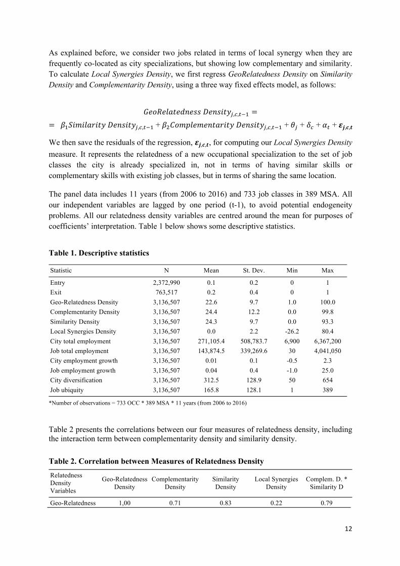
As explained before, we consider two jobs related in terms of local synergy when they are frequently co-located as city specializations, but showing low complementary and similarity. To calculate Local Synergies Density, we first regress GeoRelatedness Density on Similarity Density and Complementarity Density, using a three way fixed effects model, as follows:

CDEFDG:1D;0DHHID0H)13%,#,5<= =

= N=-)O)G:2)13ID0H)13%,#,5<=+NP(EOQGDOD01:2)13ID0H)13%,#,5<= +@% + A# +B5 +RS,T,U

We then save the residuals of the regression, RS,T,U, for computing our Local Synergies Density measure. It represents the relatedness of a new occupational specialization to the set of job classes the city is already specialized in, not in terms of having similar skills or complementary skills with existing job classes, but in terms of sharing the same location.

The panel data includes 11 years (from 2006 to 2016) and 733 job classes in 389 MSA. All our independent variables are lagged by one period (t-1), to avoid potential endogeneity problems. All our relatedness density variables are centred around the mean for purposes of coefficients’ interpretation. Table 1 below shows some descriptive statistics.

Table 1. Descriptive statistics

Statistic N Mean St. Dev. Min Max Entry 2,372,990 0.1 0.2 0 1

Exit 763,517 0.2 0.4 0 1 Geo-Relatedness Density 3,136,507 22.6 9.7 1.0 100.0 Complementarity Density 3,136,507 24.4 12.2 0.0 99.8 Similarity Density 3,136,507 24.3 9.7 0.0 93.3 Local Synergies Density 3,136,507 0.0 2.2 -26.2 80.4 City total employment 3,136,507 271,105.4 508,783.7 6,900 6,367,200 Job total employment 3,136,507 143,874.5 339,269.6 30 4,041,050 City employment growth 3,136,507 0.01 0.1 -0.5 2.3 Job employment growth 3,136,507 0.04 0.4 -1.0 25.0 City diversification 3,136,507 312.5 128.9 50 654 Job ubiquity 3,136,507 165.8 128.1 1 389

*Number of observations = 733 OCC * 389 MSA * 11 years (from 2006 to 2016)

Table 2 presents the correlations between our four measures of relatedness density, including the interaction term between complementarity density and similarity density.

Table 2. Correlation between Measures of Relatedness Density

Relatedness Density Variables

Geo-Relatedness Density

Complementarity Density

Similarity Density

Local Synergies Density

Complem. D. * Similarity D

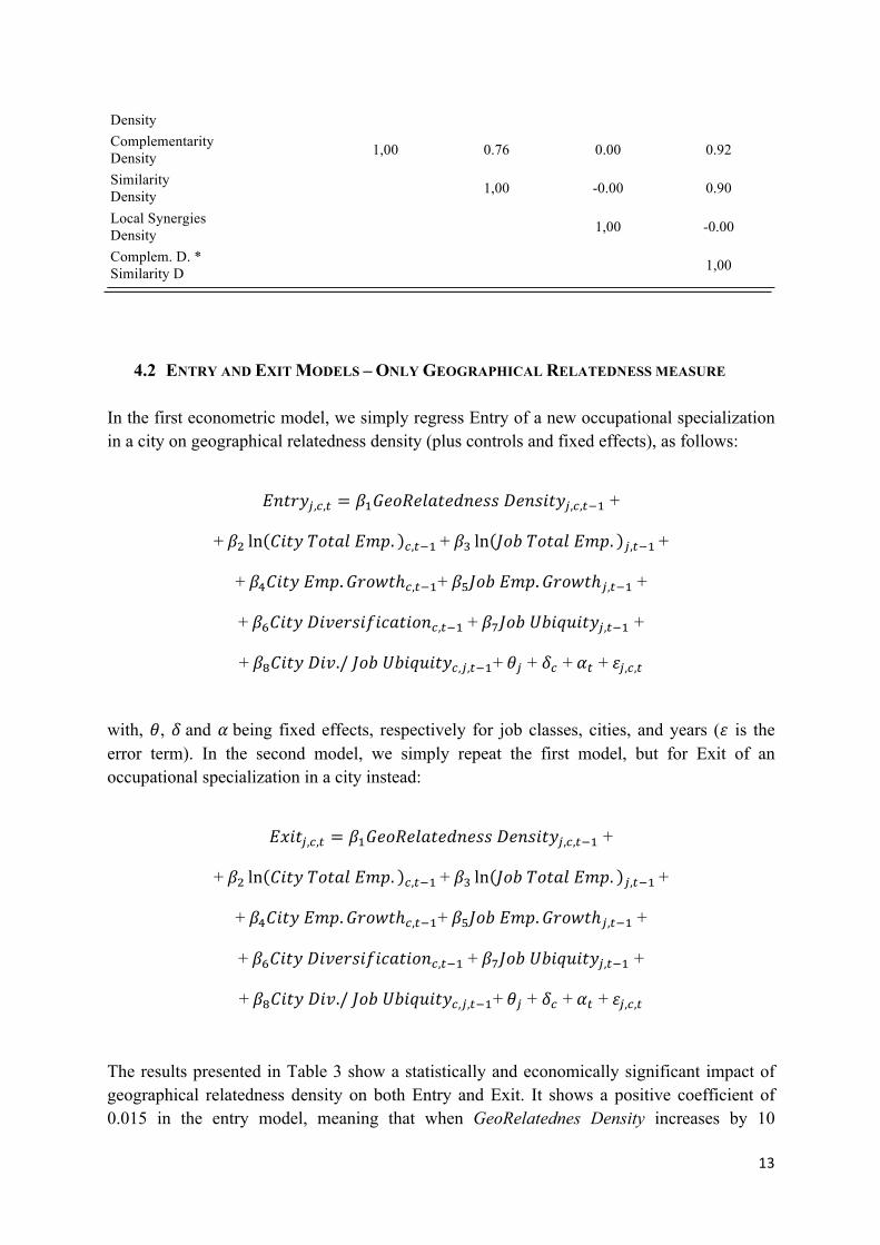
Geo-Relatedness 1,00 0.71 0.83 0.22 0.79

13

Density Complementarity Density 1,00 0.76 0.00 0.92

Similarity Density 1,00 -0.00 0.90

Local Synergies Density 1,00 -0.00

Complem. D. * Similarity D 1,00

4.2 ENTRY AND EXIT MODELS – ONLY GEOGRAPHICAL RELATEDNESS MEASURE

In the first econometric model, we simply regress Entry of a new occupational specialization in a city on geographical relatedness density (plus controls and fixed effects), as follows:

/0123%,#,5 = N=CDEFDG:1D;0DHHID0H)13%,#,5<= +

+NP ln ()13.E1:G/OQ. #,5<= +NY ln ZE[.E1:G/OQ. %,5<= +

+N\()13/OQ. C2E]1ℎ#,5<=+N_ZE[/OQ. C2E]1ℎ%,5<=+

+N`()13I)aD2H)b)c:1)E0#,5<=+NdZE[e[)fg)13%,5<= +

+Nh()13I)a./ZE[e[)fg)13#,%,5<=+@% + A# +B5 +j%,#,5

with, @, Aand Bbeing fixed effects, respectively for job classes, cities, and years (j is the error term). In the second model, we simply repeat the first model, but for Exit of an occupational specialization in a city instead:

/')1%,#,5 = N=CDEFDG:1D;0DHHID0H)13%,#,5<= +

+NP ln ()13.E1:G/OQ. #,5<= +NY ln ZE[.E1:G/OQ. %,5<= +

+N\()13/OQ. C2E]1ℎ#,5<=+N_ZE[/OQ. C2E]1ℎ%,5<=+

+N`()13I)aD2H)b)c:1)E0#,5<=+NdZE[e[)fg)13%,5<= +

+Nh()13I)a./ZE[e[)fg)13#,%,5<=+@% + A# +B5 +j%,#,5

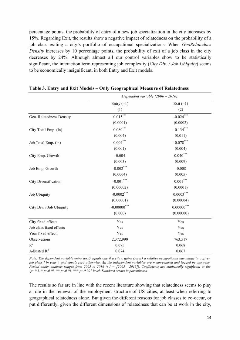
The results presented in Table 3 show a statistically and economically significant impact of geographical relatedness density on both Entry and Exit. It shows a positive coefficient of 0.015 in the entry model, meaning that when GeoRelatednes Density increases by 10

14

percentage points, the probability of entry of a new job specialization in the city increases by 15%. Regarding Exit, the results show a negative impact of relatedness on the probability of a job class exiting a city’s portfolio of occupational specializations. When GeoRelatednes Density increases by 10 percentage points, the probability of exit of a job class in the city decreases by 24%. Although almost all our control variables show to be statistically significant, the interaction term representing job complexity (City Div. / Job Ubiquity) seems to be economically insignificant, in both Entry and Exit models.

Table 3. Entry and Exit Models – Only Geographical Measure of Relatedness

Dependent variable (2006 – 2016): Entry (=1) Exit (=1)

(1) (2) Geo. Relatedness Density 0.015*** -0.024***

(0.0001) (0.0002) City Total Emp. (ln) 0.080*** -0.134***

(0.004) (0.011) Job Total Emp. (ln) 0.004*** -0.078***

(0.001) (0.004) City Emp. Growth -0.004 0.040***

(0.003) (0.009) Job Emp. Growth -0.002*** -0.008

(0.0004) (0.005) City Diversification -0.001*** 0.001***

(0.00002) (0.0001) Job Ubiquity -0.0002*** 0.0003***

(0.00001) (0.00004) City Div. / Job Ubiquity -0.00000*** 0.00000***

(0.000) (0.00000) City fixed effects Yes Yes

Job class fixed effects Yes Yes Year fixed effects Yes Yes Observations 2,372,990 763,517 R2 0.075 0.068 Adjusted R2 0.074 0.067 Note:The dependent variable entry (exit) equals one if a city c gains (loses) a relative occupational advantage in a given job class j in year t, and equals zero otherwise. All the independent variables are mean-centred and lagged by one year. Period under analysis ranges from 2005 to 2016 (t-1 = [2005 - 2015]). Coefficients are statistically significant at the ´p<0.1, * p<0.05, ** p<0.01, *** p<0.001 level. Standard errors in parentheses.

The results so far are in line with the recent literature showing that relatedness seems to play a role in the renewal of the employment structure of US cities, at least when referring to geographical relatedness alone. But given the different reasons for job classes to co-occur, or put differently, given the different dimensions of relatedness that can be at work in the city,

15

we still lack understanding of which dimensions influence the evolution of the employment structure in cities? To test this, instead of geographical relatedness density, we include our density measures for similarity, complementarity and local synergies.

4.3 ENTRY AND EXIT MODELS – ALL DIMENSIONS OF RELATEDNESS

We start by regressing Entry and Exit on each of the three dimensions of relatedness density one at a time. Then, we include them all together, plus an interaction term between Similarity Density and Complementarity Density, to account for pairs of jobs that are simultaneously similar and complementary. The complete models for Entry and Exit are as follows:

/0123%,#,5 = N=(EOQGDOD01:2)13ID0H)13%,#,5<=+NP-)O)G:2)13ID0H)13%,#,5<=+

+NY!Ec:G-30D2k)DHID0H)13%,#,5<= +

+N\-)O)G:2)13ID0H)13∗ (EOQGDOD01:2)13ID0H)13%,#,5<= +

+N_ ln ()13.E1:G/OQ. #,5<= +N` ln ZE[.E1:G/OQ. %,5<= +

+Nd()13/OQ. C2E]1ℎ#,5<=+NhZE[/OQ. C2E]1ℎ%,5<=+

+Nl()13I)aD2H)b)c:1)E0#,5<=+N=mZE[e[)fg)13%,5<= +

+N==()13I)a./ZE[e[)fg)13#,%,5<=+@% + A# +B5 +j%,#,5

/')1%,#,5 = N=(EOQGDOD01:2)13ID0H)13%,#,5<=+NP-)O)G:2)13ID0H)13%,#,5<=+

+NY!Ec:G-30D2k)DHID0H)13%,#,5<= +

+N\-)O)G:2)13ID0H)13∗ (EOQGDOD01:2)13ID0H)13%,#,5<= +

+N_ ln ()13.E1:G/OQ. #,5<= +N` ln ZE[.E1:G/OQ. %,5<= +

+Nd()13/OQ. C2E]1ℎ#,5<=+NhZE[/OQ. C2E]1ℎ%,5<=+

+Nl()13I)aD2H)b)c:1)E0#,5<=+N=mZE[e[)fg)13%,5<= +

+N==()13I)a./ZE[e[)fg)13#,%,5<=+@% + A# +B5 +j%,#,5

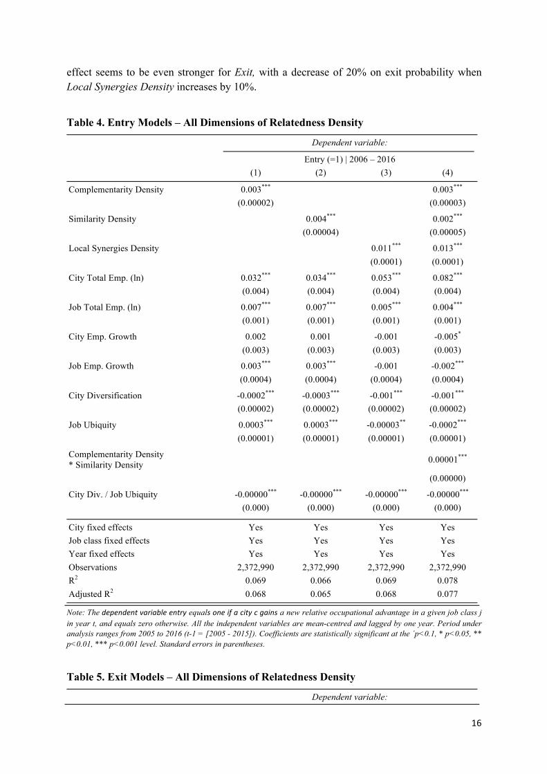
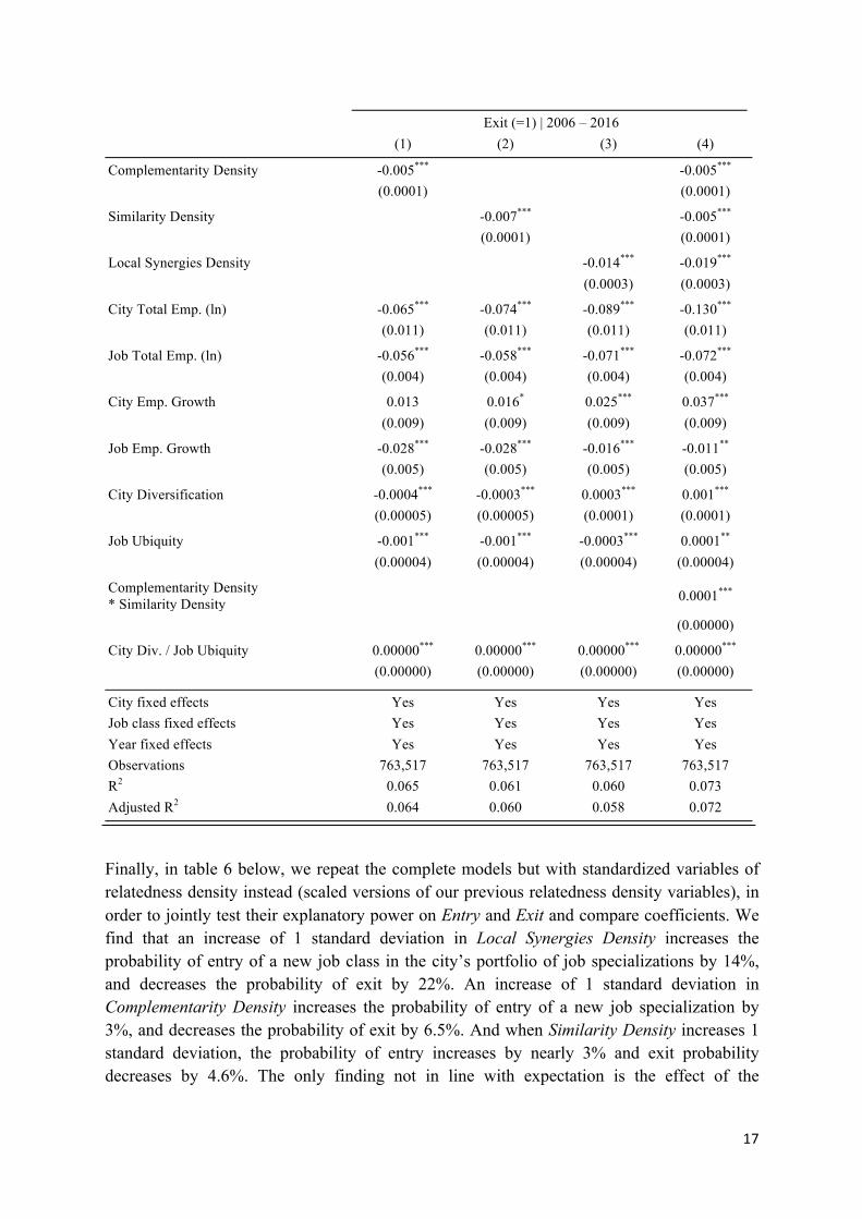
The results in Tables 4 and 5 show that each dimension of relatedness density, either alone or jointly, has a significant effect on the probability that a city specializes in a new job class or loses an existing job class. The stronger effect on Entry comes from Local Synergies Density, where an increase of 10% is associated with a 13% increase in the probability of entry. Its

16

effect seems to be even stronger for Exit, with a decrease of 20% on exit probability when Local Synergies Density increases by 10%.

Table 4. Entry Models – All Dimensions of Relatedness Density

Dependent variable: Entry (=1) | 2006 – 2016

(1) (2) (3) (4) Complementarity Density 0.003*** 0.003***

(0.00002) (0.00003) Similarity Density 0.004*** 0.002***

(0.00004) (0.00005) Local Synergies Density 0.011*** 0.013***

(0.0001) (0.0001) City Total Emp. (ln) 0.032*** 0.034*** 0.053*** 0.082***

(0.004) (0.004) (0.004) (0.004) Job Total Emp. (ln) 0.007*** 0.007*** 0.005*** 0.004***

(0.001) (0.001) (0.001) (0.001) City Emp. Growth 0.002 0.001 -0.001 -0.005*

(0.003) (0.003) (0.003) (0.003) Job Emp. Growth 0.003*** 0.003*** -0.001 -0.002***

(0.0004) (0.0004) (0.0004) (0.0004) City Diversification -0.0002*** -0.0003*** -0.001*** -0.001***

(0.00002) (0.00002) (0.00002) (0.00002) Job Ubiquity 0.0003*** 0.0003*** -0.00003** -0.0002***

(0.00001) (0.00001) (0.00001) (0.00001) Complementarity Density

* Similarity Density 0.00001***

(0.00000) City Div. / Job Ubiquity -0.00000*** -0.00000*** -0.00000*** -0.00000***

(0.000) (0.000) (0.000) (0.000) City fixed effects Yes Yes Yes Yes

Job class fixed effects Yes Yes Yes Yes Year fixed effects Yes Yes Yes Yes Observations 2,372,990 2,372,990 2,372,990 2,372,990 R2 0.069 0.066 0.069 0.078 Adjusted R2 0.068 0.065 0.068 0.077

Note:Thedependentvariableentry equalsoneifacitycgains a new relative occupational advantage in a given job class j in year t, and equals zero otherwise. All the independent variables are mean-centred and lagged by one year. Period under analysis ranges from 2005 to 2016 (t-1 = [2005 - 2015]). Coefficients are statistically significant at the ´p<0.1, * p<0.05, ** p<0.01, *** p<0.001 level. Standard errors in parentheses.

Table 5. Exit Models – All Dimensions of Relatedness Density

Dependent variable:

17

Exit (=1) | 2006 – 2016

(1) (2) (3) (4) Complementarity Density -0.005*** -0.005***

(0.0001) (0.0001) Similarity Density -0.007*** -0.005***

(0.0001) (0.0001) Local Synergies Density -0.014*** -0.019***

(0.0003) (0.0003) City Total Emp. (ln) -0.065*** -0.074*** -0.089*** -0.130***

(0.011) (0.011) (0.011) (0.011) Job Total Emp. (ln) -0.056*** -0.058*** -0.071*** -0.072***

(0.004) (0.004) (0.004) (0.004) City Emp. Growth 0.013 0.016* 0.025*** 0.037***

(0.009) (0.009) (0.009) (0.009) Job Emp. Growth -0.028*** -0.028*** -0.016*** -0.011**

(0.005) (0.005) (0.005) (0.005) City Diversification -0.0004*** -0.0003*** 0.0003*** 0.001***

(0.00005) (0.00005) (0.0001) (0.0001) Job Ubiquity -0.001*** -0.001*** -0.0003*** 0.0001**

(0.00004) (0.00004) (0.00004) (0.00004) Complementarity Density

* Similarity Density 0.0001***

(0.00000) City Div. / Job Ubiquity 0.00000*** 0.00000*** 0.00000*** 0.00000***

(0.00000) (0.00000) (0.00000) (0.00000) City fixed effects Yes Yes Yes Yes

Job class fixed effects Yes Yes Yes Yes Year fixed effects Yes Yes Yes Yes Observations 763,517 763,517 763,517 763,517 R2 0.065 0.061 0.060 0.073 Adjusted R2 0.064 0.060 0.058 0.072

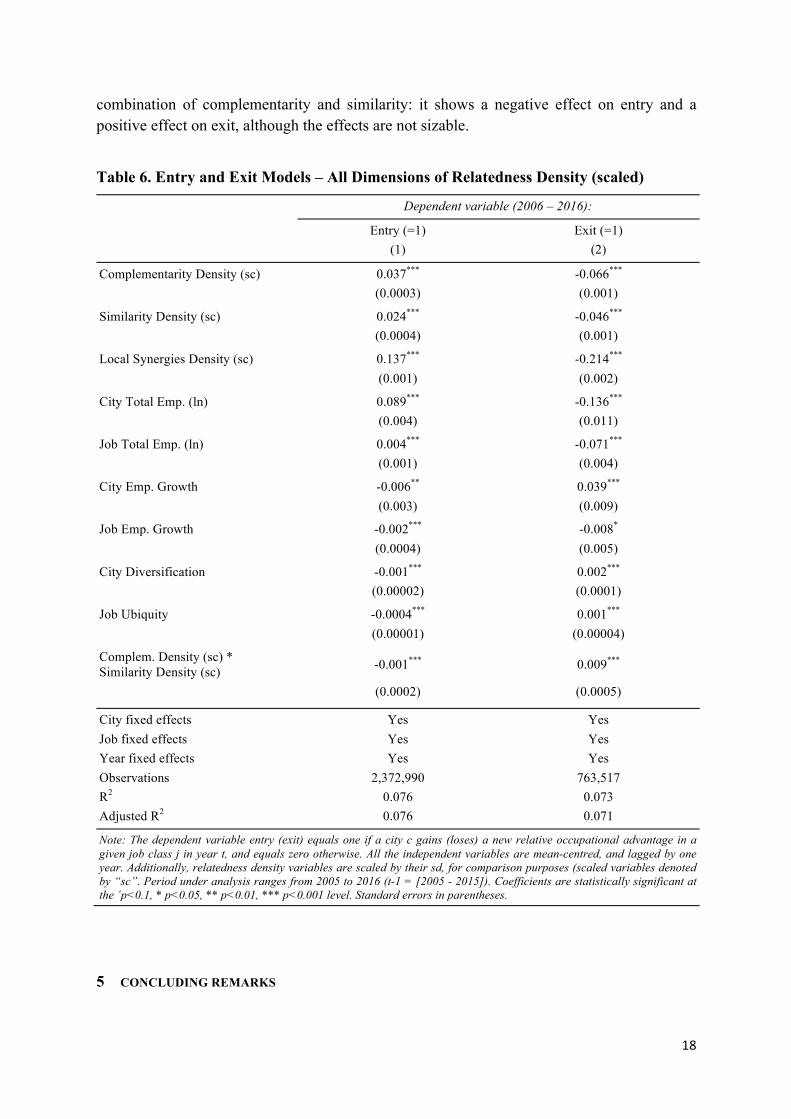
Finally, in table 6 below, we repeat the complete models but with standardized variables of relatedness density instead (scaled versions of our previous relatedness density variables), in order to jointly test their explanatory power on Entry and Exit and compare coefficients. We find that an increase of 1 standard deviation in Local Synergies Density increases the probability of entry of a new job class in the city’s portfolio of job specializations by 14%, and decreases the probability of exit by 22%. An increase of 1 standard deviation in Complementarity Density increases the probability of entry of a new job specialization by 3%, and decreases the probability of exit by 6.5%. And when Similarity Density increases 1 standard deviation, the probability of entry increases by nearly 3% and exit probability decreases by 4.6%. The only finding not in line with expectation is the effect of the

18

combination of complementarity and similarity: it shows a negative effect on entry and a positive effect on exit, although the effects are not sizable.

Table 6. Entry and Exit Models – All Dimensions of Relatedness Density (scaled)

Dependent variable (2006 – 2016): Entry (=1) Exit (=1)

(1) (2) Complementarity Density (sc) 0.037*** -0.066***

(0.0003) (0.001) Similarity Density (sc) 0.024*** -0.046***

(0.0004) (0.001) Local Synergies Density (sc) 0.137*** -0.214***

(0.001) (0.002) City Total Emp. (ln) 0.089*** -0.136***

(0.004) (0.011) Job Total Emp. (ln) 0.004*** -0.071***

(0.001) (0.004) City Emp. Growth -0.006** 0.039***

(0.003) (0.009) Job Emp. Growth -0.002*** -0.008*

(0.0004) (0.005) City Diversification -0.001*** 0.002***

(0.00002) (0.0001) Job Ubiquity -0.0004*** 0.001***

(0.00001) (0.00004) Complem. Density (sc) *

Similarity Density (sc) -0.001*** 0.009***

(0.0002) (0.0005) City fixed effects Yes Yes

Job fixed effects Yes Yes Year fixed effects Yes Yes Observations 2,372,990 763,517 R2 0.076 0.073 Adjusted R2 0.076 0.071 Note: The dependent variable entry (exit) equals one if a city c gains (loses) a new relative occupational advantage in a given job class j in year t, and equals zero otherwise. All the independent variables are mean-centred, and lagged by one year. Additionally, relatedness density variables are scaled by their sd, for comparison purposes (scaled variables denoted by “sc”. Period under analysis ranges from 2005 to 2016 (t-1 = [2005 - 2015]). Coefficients are statistically significant at the ´p<0.1, * p<0.05, ** p<0.01, *** p<0.001 level. Standard errors in parentheses.

5 CONCLUDING REMARKS

19

While many studies have looked at regional diversification into new products (Hidalgo et al. 2007), new industries (Neffke et al. 2011) or new technologies (Kogler et al. 2013; Rigby 2015), this paper has taken an occupational-network approach examining the evolution of job portfolio’s in US cities. The paper replicates the result found in other studies on the evolution of occupational structures in cities (Muneepeerakul et al. 2013; Brachert 2016; Shutter et al. 2016) that cities enter new jobs related to existing ones in cities, and exit existing jobs unrelated to their job portfolio’s. What is new about this paper is that we have unpacked three mechanisms through which the entry and exit of jobs in cities takes place. While previous papers looked at the effect of geographical relatedness only, we unravel three mechanisms through which the effect of geographical relatedness might work because co-location of jobs does not tell us much about the forces that make jobs co-occur in the same city: new local jobs may be related to existing local jobs because they share similar skills or provide complementary tasks, or both, or because they benefit from being co-located.

First, we constructed a job space that represents a network of interdependent job classes that includes the three dimensions through which jobs may be related to each other. In doing do, we can unravel links between pairs of jobs in terms of being similar, being complementary, being both similar and complementary, or in terms of sharing local synergies. Second, we investigated the importance of each of these three job relatedness dimensions for the evolution of jobs in 389 US cities for the period 2005-2016. For this purpose, we introduced a new methodological approach to distinguish between the three relatedness effects.

The main finding is that all three relatedness dimensions (similarity, complementarity and local synergies) increase the chances of entry of a new job in a city on the one hand, and decrease the probability of disappearance of an existing job in a city on the other hand. Moreover, we found the negative effect of relatedness on exits of jobs to be stronger than the positive effect of relatedness on entry of jobs: all three relatedness dimensions seem to prevent exit of jobs in cities more than promoting entry of jobs in cities. The local synergy density effect shows the largest effect on both entry and exit: this outcome suggests that the stronger local synergies across job classes are, the greater the effect on diversification and the harder to dislocate existing job classes. The complementarity density effect reflects the tendency of an increasing division of labour in cities which brings higher levels of interdependence between job specializations (Shutters et al. 2018) where each worker’s productivity depends on whether or not she has access to co-workers with specialized skills and know-how that complement her own (Neffke 2017). The similarity density effect found is in line with the tendency of firms and people to cluster geographically to benefit from a pool of labour with related skills (Neffke and Henning 2013). Similarity seems to prevent exit and promote entry of jobs in cities, but not in combination with complementarity.

Although this paper provides an important step to unpack relatedness, it is still far from comprehensive (Boschma 2017). First, while we have started to unravel the geographical density effect (controlling for similarity and complementarity), there is a need to investigate what the local synergies dimension consists of. Second, we need more studies in other countries to shed more systematic light on the importance of the different relatedness dimensions. Third, the three dimensions of relatedness density might play different roles

20

depending on the level of knowledge complexity of activities (Balland and Rigby, 2017) and should be employed and tested in studies on regional diversification into new products, industries or technologies, besides new jobs. Finally, we have to make an effort to include institutions in this framework, because regional diversification might also be affected by institutional requirements that different jobs, industries or technologies have in common (Boschma and Capone 2015).

6 REFERENCES

Autor, D. (2010), “The Polarization of Job Opportunities in the U.S. Labor Market: Implications for Employment and Earnings.” Center for American Progress and the Hamilton Project.

Balland, P.A., Boschma, R., Crespo, J. and Rigby, D. (2018), “Smart Specialization policy in the EU: Relatedness, Knowledge Complexity and Regional Diversification”, Regional Studies, forthcoming.

Balland, P.A. and Rigby, D. (2017), “The Geography of Complex Knowledge”, Economic Geography, 93 (1), 1-23

Barbour, E., and Markusen, A. (2007), “Regional occupational and industrial structure: Does the one imply the other?” International Regional Science Review, 29 (1), 1-19.

Boschma, R. (2017) Relatedness as driver behind regional diversification: a research agenda, Regional Studies 51 (3), 351-364.

Boschma, R., Balland, P.A., and Kogler, D. (2015), “Relatedness and technological change in cities: the rise and fall of technological knowledge in U.S. metropolitan areas from 1981 to 2010”, Industrial and Corporate Change, 24, 223–250.

Boschma, R. and G. Capone (2015) Institutions and diversification: Related versus unrelated diversification in a varieties of capitalism framework, Research Policy 44, 1902-1914.

Boschma, R., Minondo, A., Navarro, M. (2013) The emergence of new industries at the regional level in Spain. A proximity approach based on product-relatedness, Economic Geography 89 (1), 29-51

Boschma, R.A. and K. Frenken (2006), “Why is economic geography not an evolutionary science? Towards an evolutionary economic geography”, Journal of Economic Geography 6 (3), 273-302.

Brachert, M. (2016) The rise and fall of occupational specializations in German regions from 1992 to 2010. Relatedness as driving force of human capital dynamics, working paper.

Breschi, S., Lissoni, F., & Malerba, F. (2003), “Knowledge-relatedness in firm technological diversification”. Research Policy 32 (1), 69-87.

21

Duranton, J., and Puga, D. (2003). Micro-foundation of urban agglomeration economies in Henderson V. J. and Thisse JF.(eds) Handbook of Regional and Urban Economics Vol. 4 Cities and Geography.

Eck, N. J. V., and Waltman, L. (2009), “How to normalize cooccurrence data? An analysis of some well- known similarity measures”, Journal of the American Society for Information Science and Technology, 60(8), 1635-1651.

Essleztbichler, J. (2015) Relatedness, industrial branching and technological cohesion in US metropolitan areas, Regional Studies 49 (5), 752–766.

Feser, E. (2003), “What regions do rather than make: A proposed set of knowledge-based occupation clusters”, Urban Studies 40 (10), 1937 - 1958

Florida, R. (2002). “The economic geography of talent”. Annals of the Association of American Geographers 92 (4), 743-755.

Frenken, K., Oort, F., and Verburg, T. (2007). "Related Variety, Unrelated Variety and Regional Economic Growth," Regional Studies, 41 (5), 685-697.

Gereffi, G., and Korzeniewicz, M. (1994) (eds) Commodity Chains and Global Capitalism, Westport, CT.: Praeger.

Hasan, S., Ferguson, J. P., and Koning, R. (2015). “The Lives and Deaths of Jobs: Technical Interdependence and Survival in a Job Structure”. Organization Science, Articles in Advance. Catonsville: Informs (doi 10.1287/orsc.2015.1014).

Hausmann, R., and Hidalgo, C. (2010). "Country Diversification, Product Ubiquity, and Economic Divergence," Working Paper Series rwp10-045, Harvard University, John F. Kennedy School of Government.

He, C., Guo, Q., and Rigby, D. (2015), “Industry Relatedness, Agglomeration Externalities and Firm Survival in China”, Papers in Evolutionary Economic Geography (PEEG), Utrecht University, Department of Human Geography and Spatial Planning, Group Economic Geography. https://EconPapers.repec.org/RePEc:egu:wpaper:1528

Hidalgo, C., Klinger, B., and Barabasi, A. (2007), “The product space conditions the development of nations”. Science 317 (5837), 482-487.

Kogler, D. F., D. L. Rigby and I. Tucker (2013), “Mapping knowledge space and technological relatedness in U.S. cities”, European Planning Studies, 21 (9), 1374–1391.

Markusen, A., Wassall, G. H., DeNatale, D., and Cohen, R. (2008). Defining the creative economy: Industry and occupational approaches. Economic Development Quarterly, 22 (1), 24-45.

Markusen A. and Schrock, G. (2006), “The Distinctive City: Divergent Patterns in Growth, Hierarchy and Specialization”. Urban Studies, 43 (8), 1301-23.

Markusen, A. (2004) “Targeting Occupations in Regional and Community Economic Development.” 2004. Journal of the American Planning Association, 70 (3), 253-68.

22

Markusen, A., Chapple, K., Schrock, G., Yamamoto, D., and Yu, P. (2001), High-tech and I-tech: how metros rank and specialize, Minneapolis, MN: The Hubert H. Humphrey Institute of Public Affairs.

Martin, R., and Sunley, P., (2006), "Path Dependence and Regional Economic Evolution", Papers in Evolutionary Economic Geography (PEEG) 0606, Utrecht University, Department of Human Geography and Spatial Planning, Group Economic Geography.

Mehta, A. (2014). “5 Ways to Lessen Inequality as Demand for Labor Decreases Worldwide”, http://www.huffingtonpost.com/aashish-mehta/5-ways-lesson-inequality_b_6215708.html

Moretti, E. and Kline, P. (2014), "Local Economic Development, Agglomeration Economies and the Big Push: 100 Years of Evidence from the Tennessee Valley Authority", Quarterly Journal of Economics, 129 (1).

Moretti, E. (2013) “Real Wage Inequality" American Economic Journal: Applied Economics, 5 (1).

Moretti, E. (2012) The New Geography of Jobs. New York: Houghton Miffin Harcourt.

Muneepeerakul, R., Lobo, J., Shutters, S., Gomez-Lievano, A., and Qubbaj. M. (2013), “Urban economies and occupation space: can they get “there” from “here”?” PLoS ONE 8(9): e73676. doi: 10.1371/journal.pone.0073676.

Neffke, F., (2017), “Coworker Complementarity”. SWPS 2017-05. Available at SSRN: https://ssrn.com/abstract=2929339 or http://dx.doi.org/10.2139/ssrn.2929339

Neffke, F., and Henning, M. (2013), “Skill relatedness and firm diversification”, Strategic Management Journal, 34(3), 297-316.

Neffke F, Henning M, and Boschma R (2011), “How do regions diversify over time? Industry relatedness and the development of new growth paths in regions”. Economic Geography 87: 237–265.

Petralia, S., Balland, P.A., and Morrison, A. (2017), “Climbing the Ladder of Technological Development”, Research Policy, 46 (5): 956–969.

Renski, H., Koo, J., & Feser, E. (2007). Differences in labor versus value chain industry clusters: An empirical investigation. Growth and Change, 38(3), 364-395.

Rigby, D., (2015), “Technological Relatedness and Knowledge Space: Entry and Exit of U.S. Cities from Patent Classes”, Regional Studies, 49 (11), 1922-1937.

Rodriguez, F., and Jayadev, A. (2010), “The Declining Labor Share of Income”. Human Development Reports Research Paper, no. 2010/36.

Shutters, S., Lobo, J., Muneepeerakul, R., Strumsky, D., Mellander, C., Brachert, M., Farinha-Fernandes, T., and Bettencourt, L. (2018), “Urban Occupational Structures as Information Networks: Scaling of Network Density with Number of Occupations”, working paper.

23

Shutters, S., Muneepeerakul, R., and Lobo, J. (2016), “Constrained pathways to a creative urban economy”, Urban Studies 53(16):3439-3454

Shutters, S., Muneepeerakul, R. and Lobo, J. (2015) “Quantifying urban economic resilience through labour force interdependence.” Palgrave Communications 1:15010 doi: 10.1057/palcomms.2015.10.

Shutters, S., Muneepeerakul, R., and Lobo, J. (2015), “Constrained pathways to a creative urban economy”. Martin Prosperity Research. Retrieved October 20, 2015, from http://martinprosperity.org/media/WP2015_Constrained-pathways-to-a-creative-urban-economy_Shutters-Muneepeerakul-Lobo.pdf

Steijn, M.P.A. (2018), “Improvement on the association strength: implementing a probabilistic measure based on combinations without repetition”. (forthcoming)

Tanner, A. N. (2014), Regional Branching Reconsidered: Emergence of the Fuel Cell Industry in European Regions. Economic Geography, 90: 403–427. doi:10.1111/ecge.12055

Thompson, W. R., and Thompson, P. R. (1987). “Alternative paths to the revival of industrial cities. In G. Gappert (Ed.)”, The Future of Winter Cities. Newbury Park, CA: Sage.

Thompson, W. R., and Thompson, P. R., (1985). “From Industries to Occupations: Rethinking Local Economic Development.” Economic Development Commentary, Vol. 9.

US Census Bureau. (2015), “Metropolitan and Micropolitan Statistical Areas”. Available at: www.census.gov/population/metro/.