Russell Sage 1

What Does Increased Economic Inequality Imply about the Future Level and Dispersion of Human Capital?

Mary Campbell Robert Haveman Gary Sandefur Barbara Wolfe

University of Wisconsin–Madison

May 6, 2004

We thank the Russell Sage Foundation and its program on the Social Dimensions of Inequality for support for this research. Special thanks to Andrea Voyer for her insights and help thinking through dilemmas as they arose, to Susan Mayer for providing us with state gini coefficients and to Kathryn Wilson for calculating models for us that include measure of school district expenditures. We are very grateful for everything they have added to our study and for their generous willingness to share both their time and their effort. The authors are listed in alphabetical order; all contributed equally to the paper.

Russell Sage 2

Abstract

Does the well-recognized increase in economic inequality among families and neighborhoods

have implications for children who have experienced this development? Are children growing up in a

more unequal economic environment likely to choose less human capital investment (schooling) than they

would if the economic environment were more equal? Or, might a higher level of economic inequality be

related to more schooling (reflecting greater implicit returns to schooling)? Is the disparity in levels of

schooling of a cohort growing up in a more unequal environment likely to be more or less than that of a

cohort reared in a less unequal environment?

In this study we attempt to shed light on these questions. We estimate a stylized model of

children’s attainments using longitudinal data on about 1200 children from the Panel Study of Income

Dynamics. We observe these children over a period of at least 20 years, and statistically estimate the

relationship of the family and regional/neighborhood factors that exist while they are growing up to the

educational choices that they make when young adults. Our human capital variables are completed years

of schooling, graduation from high school and college attendance. The family and neighborhood/regional

economic variables inequality are family income (relative to needs), family net worth (wealth), a state

measure of inequality (the Gini coefficient), and a measure of the accessibility of higher education (the

cost of tuition at state colleges).

We then use the estimated relationships to simulate the effects of changes in the inequality of

family and neighborhood/regional economic variables on the level of youth schooling attainments. We

indicate the effects of changes in economic inequality of the family and regional/neighborhood variables

on both the average level of educational attainment of our cohort of youths, and on the inequality among

these youths in educational attainment.

We conclude that increases in the inequality of economic circumstances of both families and

regions/neighborhoods will have small but slightly positive effects on the average level of schooling.

However, increased inequality in family and regional/neighborhood circumstances is associated with

substantial increases in the inequality of schooling attainments among these youths.

Russell Sage 3

The past three decades have witnessed substantial growth in economic inequality among families.

For example, between 1973 and 1998, the gini coefficient of income among families rose from .356 to

.430, an increase of 21 percent (see Haveman, Sandefur, Wolfe, and Voyer, 2001). This increase in family

income inequality reflects the net effect of changes in inequality of labor market attainments (wage rates,

working time)1 and public income transfers.

Growing inequality among the geographic areas in which people live—and hence the social

isolation of economic and racial/ethnic groups—has also been studied. Jargowsky (1997) has documented

the social decline in the urban neighborhoods in which many poor and minority children are concentrated,

and Massey (1996) shows that both affluence and poverty became more concentrated between 1970 and

1990.2 Given the conjectures of economists and sociologists concerning the adverse effects on children’s

attainments of growing up in low quality family and neighborhood environments, these trends in

between-jurisdiction inequality are of concern.

In this paper, we explore the relationship between the growth in economic inequality (in both

family and geographic dimensions) and the disparity among youths in their educational attainments. We

study human capital indicators of children’s attainments—the years of completed schooling that they

attain, the probability that they will graduate from high school and the probability they will attend college

or another form of post-secondary schooling. We relate changes in the level and the dispersion of

schooling attainment among a group of young adults to changes in the level of inequality in family

economic position and regional economic performance that may occur during the years when they were

growing up (ages 2–15).

Our analysis rests on two primary conjectures. First, we expect that higher levels of inequality in

family and neighborhood/regional circumstances while growing up will be associated with lower average

1For example, the inequality of both female and male full-time worker earnings increased by nearly 30

percent over the 1975 to 2000 period. 2In fact, affluence (persons living in families with an income at least four times the poverty line for a family

of four) is more concentrated than poverty. In 1990, the average affluent person lived in a neighborhood in which over 50 percent of his neighbors were also affluent while the average poor person lived in a neighborhood in which just over 20 percent of his neighbors were poor.

Russell Sage 4

levels of educational attainment.3 This conjecture reflects findings from numerous studies of deleterious

effects of inequality on a variety of social performance measures (See Adler et al., 1994; Marmot et al.,

1991; Diez-Roux et al., 1997; Kawachi and Kennedy 1997). Second, we expect a positive and robust

relationship between both family and neighborhood/regional economic circumstances and measures of

children’s attainments, reflecting the numerous studies of intergenerational linkages in attainments (See

Haveman and Wolfe, 1994, 1995, McLanahan and Sandefur, 1994, and more recently Haveman,

Sandefur, Wolfe, and Voyer, 2001). Because of this relationship, we expect increased inequality in both

family and neighborhood/regional economic characteristics to be associated with greater schooling

disparities among youth.

Mayer (2001) has explored the relationship between inequality in family and regional

circumstances while children are growing up with the level and the disparity in economic attainments

among them during young adulthood. Using data from the Michigan Panel Survey of Income Dynamics

(PSID), she estimates the relationship between state-level economic inequality during adolescence and

eventual educational attainment, distinguishing potentially differential impacts on rich vs. poor children.4

Within-state inequality is measured by a gini coefficient calculated over family income using data from

the decennial census, interpolated linearly to obtain a state inequality measure for each observation at age

14. Control variables include estimated measures of returns to education, region, year, percentage of the

state population that is African-American and Hispanic, mean within-state household income, and

unemployment rate, the log of family income, and a measure of economic segregation within the state.

Separate estimates are made over high- and low-income observations, defined as living in a family above

or below the median level of family income (at ages 12–14).

3This effect may be mitigated in that decreases in educational attainment may be constrained by legal and institutional factors (e.g., mandatory school attendance regulations), while choices involving additional schooling (e.g., college attendance) are less so.

4Mayer’s sample of children consists of all observations in the data set at ages 12–14, and ages 20 and 23 (when the relevant educational outcome data were available). Measures of within-state economic inequality and control variables were obtained when the respondents were between the ages of 12 and 14. Mayer considers four educational outcomes: the probability of high school completion by age 20; the probability of beginning college by age 23; the probability of completing four years of post-secondary education by age 23; and the number of years of completed schooling by age 23.

Russell Sage 5

While Mayer finds very low zero-order correlations between the state ginis and the educational

outcomes—less than -.04 for each outcome—changes in within-state income inequality are positively

related to the educational attainment of higher income children, and negatively related to that of lower

income children in multivariate estimates. She finds that mean educational attainment increases as within-

state income inequality increases. Significant positive coefficients on within-state income inequality are

estimated for higher income observations when years of education (with the base set of controls) and for

college graduation (after adding controls for state educational policies) are dependent variables. Among

lower income respondents, within-state income inequality is significantly and negatively related to only

the years-of-schooling variable.

Mayer concludes that increased within-state inequality is associated with increased overall

educational attainment (primarily due to increasing post-secondary education entrance choices) and

increased inequality in youth educational attainment. Variables reflecting changes in returns to education,

parental income and state-level investments in education are positively related to youth educational

inequality, as these effects tend to be concentrated on youth from higher-income families.

Our study addresses a similar question. We also relate hypothesized changes in a variety of

dimensions of family and geographic inequality to both the average level and the dispersion of children’s

educational attainment. However, rather than relating only changes in within-state inequality to

educational attainments, we directly alter—through simulation analysis—the level of inequality among

the families of children (family income/needs, wealth) and among the states in which children live (as

measured by state-specific gini coefficients of family income/needs and the level of in-state higher

education costs).5 The other unique features of our study are the inclusion of data over nearly all years of

5While Mayer relates changes in mean educational attainment to within-state income inequality, we adjust

family income/needs, wealth, and across-state inequality and higher education costs back to the original mean, and then test how changes in these variables influence the mean and distribution of youth educational outcomes. Mayer suggests that increased returns to schooling contribute to increased income inequality, and hence the level of educational attainment. However, she argues that redistribution of income from the rich to the poor will increase mean educational attainment more than would an equivalent increase in incomes across the distribution, provided the relationship between family income and educational attainment is semi-logarithmic. If a semi-logarithmic relationship between family income/needs (and wealth and state income inequality and education costs) and

Russell Sage 6

a child’s life (e.g., family characteristics beginning at the child’s age 2), data measuring the childcare

experiences of the child, information that tracks all the locations a child has lived, and a direct measure of

the cost of post-secondary schooling.

In Section I, we briefly describe the research strategy on which our analysis rests. In effect, we

model the relationship of relevant family and regional/neighborhood characteristics observed for a sample

of children while they were growing up to their educational attainments when they are young adults. We

also describe the data set that we use for the analysis in this section. Section II summarizes the findings

from our analysis in a series of figures and summary measures of levels and disparities among children in

the years of schooling attained. The final section concludes.

I. RESEARCH STRATEGY AND DATA

In this analysis, we view the schooling choices of youths to be the outcome of a production

process in which both parental choices (or family circumstances) and regional/neighborhood

characteristics influence youth outcomes.6 We estimate the relationship between these family and

regional/neighborhood variables measured for a large sample of children during the childhood years (ages

2–15) to their educational attainments when they become young adults. We use a sparse model that is

motivated by the identification of those relevant family and regional/neighborhood characteristics

variables that are persistently found to be significantly related to years of schooling in the existing

research literature.7

Our basic data set consists of 21 years of information on 2609 children from the Michigan Panel

Survey of Income Dynamics (PSID). We selected children who were born from 1966 to 1970, and follow

educational attainment exists, increasing the dispersion of family income/needs by a fixed percentage (as we do) will leave the mean unchanged.

6Haveman and Wolfe (1994, 1995) discuss the implications of this framework for empirical estimation. In some formulations, youth choices are modeled as a response to incentives, with family and neighborhood environment having both direct effects on outcomes, and indirect effects through their influence on incentives. See Haveman, Wolfe, and Wilson (1997).

7In Haveman, Sandefur, Wolfe, and Voyer (2001), we present the results of a review of this literature.

Russell Sage 7

them from 1968, the first year of the PSID (or their year of birth, if later) until 1994–1999. Only those

individuals who remained in the survey until they reached age 21 are included.8 After omitting

observations with missing information in core variables, we have a sample of 906–1210 children

(depending on the outcome of interest), each of whom is observed over a period of at least 21 years.

Our data set contains extensive longitudinal information on the status, characteristics, and choices

of family members, family income (by source), living arrangements, neighborhood characteristics, and

background characteristics such as race, and location for each individual. In order to make comparisons of

individuals with different birth years, we index the time-varying data elements in each data set by age:

that is, rather than have the information defined by the year of its occurrence (say, 1968 or 1974), we

convert the data so that this time-varying information is assigned to the child by the child’s age. Hence,

we are able to compare the process of attainment across individuals with different birth years. All

monetary values are expressed in 1993 dollars using the Consumer Price Index for all items.

We merged Census tract (neighborhood) information from the 1970 and 1980 Censuses onto our

PSID data. The Census data are matched to the specific location of the children in our sample for each

year over the years 1968–1985.9 Based on this link, we are able to include in our data information

describing a variety of social and economic characteristics of rather narrowly defined areas for each

8Some observations did not respond in an intervening year but reentered the sample the following year.

Such persons are included in our analysis, and the missing information was filled in by averaging the data for the two years contiguous to the year of missing data. For the first and last years of the sample, this averaging of the contiguous years is not possible. In this case, the contiguous year’s value is assigned, adjusted if appropriate using other information that is reported. Studies of attrition in the PSID find little reason for concern that attrition has reduced the representativeness of the sample. See Becketti et al. (1988), Lillard and Panis (1994), and Haveman and Wolfe (1994). A more recent study by Fitzgerald, Gottschalk, and Moffitt (1998) finds that, while “dropouts” from the PSID panel do differ systematically from those observations retained, estimates of the determinants of choices such as schooling and teen nonmarital childbearing estimated from the data do not appear to be significantly affected.

9The links between the neighborhood in which each family in the PSID lives and small-area (census tract) information collected in the 1970 and 1980 Census have been (painfully and painstakingly) constructed by Michigan Survey Research Center (SRC) analysts. For the years 1968 to 1970, the 1970 Census data are used in this matching; for the years 1980 to 1985, the 1980 Census data are used. In most cases, this link is based on a match of the location of our observations to the relevant Census tract or block numbering area (67.8 percent for 1970 and 71.5 percent for 1980). For years 1971 to 1979, a weighted combination of the 1970 and 1980 Census data are used. The weights linearly reflect the distance from 1970 and 1980. For example, the matched value for 1972 equals [(.8 x 1970 value) + (.2 x 1980 value)].

Russell Sage 8

family in our sample, based on their residence in each of the years from 1968 to 1985.10 In this paper we

use the variables for percent who are high school drop outs and percent in the neighborhood with low

incomes.

From these data, we can also observe a number of measures of educational attainment when a

young adult for each of the children in our sample. We concentrate on three such outcomes—years of

completed schooling, completion of high school, and college attendance—all measured as of age 25.

We have selected four family and neighborhood/regional variables for our exploration of the

effects of changes in inequality on educational attainments. They are:

• Logarithm of the ratio of the income of the family in which the child grew up to the

poverty line for the family,

• Level of Net Worth of the family in which the child grew up,

• Gini coefficient for the state in which the child grew up11, and

• Cost of state tuition and fees in the state in which the child lived in 1985–1990.12

Table 1 provides unweighted descriptive statistics on all of the variables included in our models.

Three-fourths of our sample youth graduated from high school, nearly thirty percent attended college and

they have a mean educational attainment of 12.18 years of schooling. The corresponding weighted values

10These characteristics include racial composition, measures of family income and its distribution

(including the proportion of families with incomes below $10,000 and those above $15,000), the proportion of persons living in poverty, the proportion of young adults who are high school dropouts, the adult and male unemployment rates, the proportion of families that are female headed, the proportion of those in the labor force in managerial (professional) occupations, and an underclass count (See Rickets and Sawhill, 1988).

11If a child moved over ages 12–15, the gini coefficient is a weighted average of the states that the child lived in where the weights are the years lived in each state.

12The income variable is measured over the child’s ages 2–15 and included as averages over the preschool years (2–5), elementary school years (6–11) and secondary school years (12–15); the wealth indicator is measured in 1984 when the youth are age 14–18. The gini coefficient of the state where the child lived (averaged over ages 12–15, the age when our tests found that there was the greatest impact on outcomes) and the cost of tuition and fees of the public higher education institutions in the state in which they live (measured in 1987, when the youth were ages 17–21) are neighborhood/geographic variables. Our measure of the gini coefficient is that used by Susan Mayer (2001). We also planned to explore the effect of changes in the average income of the neighborhood in which the child grew up over ages 2–15. However in numerous estimates of the effect of a variety of factors on years of schooling, these neighborhood variables were never statistically significant.

Russell Sage 9

are 84 percent graduated high school, nearly 40 percent attended college and mean years of schooling

were 12.63.

II. THE EFFECTS OF FAMILY AND NEIGHBORHOOD/REGIONAL ECONOMIC CIRCUMSTANCES ON EDUCATIONAL ATTAINMENT

In assessing the effects of increases in the inequality of family and neighborhood/geographic

economic circumstances on children’s schooling attainments, we statistically relate these characteristics to

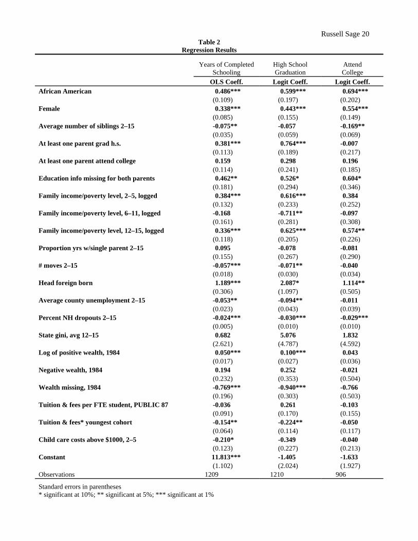
years-of-completed-schooling, high school graduation, and college attendance. Results from our

estimated models are shown in Table 2.

Our review of the numerous studies of the determinants of children’s attainments available in the

literature (See Haveman, Sandefur, Wolfe, and Voyer, 2001) identified those variables whose relationship

to attainments is persistent, robust and statistically significant. Such variables include parental schooling

attainments, family economic resources (family income and wealth), family structure (for example,

growing up in a single parent family), and the number of geographic moves during childhood. We have

supplemented these with variables describing neighborhood and state circumstances. More specifically

we have measures at the county level (unemployment rate), the neighborhood or census tract level

(percent of individuals who drop out of high school and percent in the neighborhood in low income

families), and at the state level (the state gini coefficient and public tuition and fees). Our estimate

distinguishes the race and gender of the observations. In addition, given the renewed interest in young

children’s experiences we include a variable indicating whether or not more than $1000 was spent on

childcare from ages 2 to 5 as a proxy for having spent extended periods in non-family childcare. The

model we have selected includes all the substantively relevant variables.

The estimated relationships in Table 2 are generally as expected. After controlling for family and

location characteristics, African Americans have higher educational attainment than others, and women

have higher educational attainment than men.13 Women have higher educational attainment than men

13The positive effect of being African-American after controls is a common finding in studies of

educational attainment.

Russell Sage 10

before and after controls. Individuals from families where the head is foreign born also have higher levels

of educational attainment.

Parental schooling is positively and significantly related to years of completed schooling and high

school graduation. Surprisingly, parental education is not significantly associated with college attendance

after controlling for other variables.14 In this model the effects of parental education occur through its

effects on family income and family wealth. Family income at ages 2–5 and at ages 12–15 is significantly

associated with years of completed schooling while family income at ages 6–11 is not. We see similar

effects of family income at ages 2–5 and 12–15 on high school graduation whereas family income at ages

6–11 is negatively associated with high school graduation. Only the measure of income for children at

ages 12–15 is significantly associated with college attendance.15 These results provide some evidence to

support other research that appears to show that incomes during early childhood and adolescence are

important determinants of educational attainment, and that family income during adolescence is most

important in determining college attendance.16 Wealth is strongly associated with years of completed

schooling and high school graduation, but not with college attendance. These results imply that wealth

affects college attendance and years of completed schooling through both its effect on high school

graduation and its association with family income during the adolescent years. These results suggest that

family socioeconomic status is strongly associated with educational attainment.

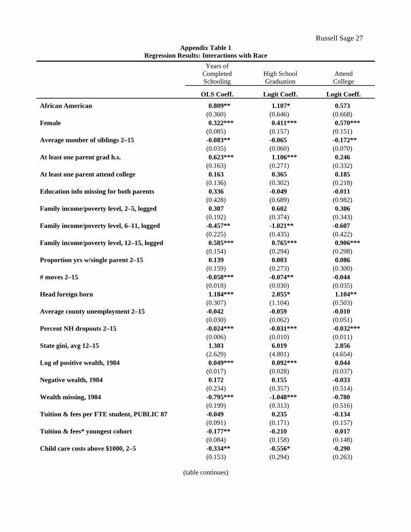
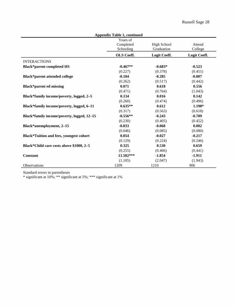
14We also estimated models in which we specified interactions between race and parental education, an

equation that also included interactions between race and income, unemployment, childcare and tuition and fees (see Appendix Table 1). The only significant interaction between race and parental education was between race and at least one parent graduating from high school in the years of education and high school graduation models. The interaction effect suggested that this variable had a smaller effect for Blacks than for Whites.

15One must be cautious in interpreting these effects, however, since the measures of family income at the different ages have correlations ranging from .75 (2–5 and 12–15) and .86 (6–11 and 12–15).

16The interactions between the income/poverty measure at ages 6–11 and race in the models that included race and income interactions (see note 14) were significant in the years of schooling models. The interactions suggested that the ratio of income to the poverty line at ages 6–11 had a positive effect on years of education for blacks but a negative effect for whites, while the income/poverty ratio at ages 12–15 had a positive effect for whites, but no effect for blacks. The interaction between the ratio of income to poverty at ages 6–11 and race was also significant in the model for attending college. This interaction indicated that the income/poverty measure had positive effects on college attendance for blacks but not for whites.

Russell Sage 11

The proportion of years that a child has lived with a single parent is not associated with any of the

three educational outcomes. Having lived with a single parent is associated with educational attainment

before controls but its effects are not significant after controlling for the socioeconomic attributes of the

family. The average number of siblings living at home over the course of childhood is associated with

years of education and college attendance but not with high school graduation. The number of residential

moves during childhood, on the other hand, is associated (negatively) with years of completed schooling

and high school graduation, but not with college attendance. Having spent considerable time in formal

childcare as a 2–5 year old is negatively associated with years of completed schooling but not with high

school graduation, or college attendance.17 If we interpret this together with results for higher income

while 2–5, it suggests that the positive association of higher income (due in part to greater work effort) is

partly offset by the negative association of formal childcare.

Finally we look at characteristics of the areas in which people live. We begin with indicators of

the neighborhood in which individuals live. These results show that each schooling outcome is negatively

associated with the percent of the neighborhood that has dropped out of high school. Our county-level

indicator—the average county unemployment rate—is significantly associated with years of completed

schooling and high school graduation, but not college attendance. The state gini is not significantly

associated with any of the educational outcomes. The tuition and fees for attending a public institution in

the state are significantly associated with high school completion and years of completed schooling but

not with college attendance. These effects are reflected in the interaction terms that suggest tuition costs

affect the outcomes for those individuals for which the tuition costs were measured closest to when they

were in their last year of high school.18

17The model that includes race interactions suggests the negative association between considerable formal

child care and education outcomes is only significant for whites. For whites the associate is significant for both years of schooling and whether or not a child graduates from high school.

18In estimates not reported here, we also included a variable measuring school expenditures per pupil. This required a trade-off as the data set to which we could match school expenditures was a slightly different population for whom we only had data beginning at age 6. Estimates from this sample, conducted by Kathryn Wilson, suggested a positive, insignificant and small association between school district expenditures and the educational outcomes.

Russell Sage 12

While most of these results are as expected, two comments are in order. First the lack of effects of

some key variables on college attendance may be due, at least in part, to the inclusion of only of

individuals who have completed high school in this part of the analysis. Further, some variables affect

college attendance through their effects on high school graduation. Second, unlike Mayer (2001) we do

not find any significant effects of the state ginis on educational outcomes in the Table 2 estimates, or

when we separately analyzed the high-income and low-income sub-samples. The differences in our

results and those of Mayer are in part due to the smaller sample that we use, but also suggest that the

effects of characteristics such as state ginis with very low correlations with educational outcomes are very

sensitive to model specification.

III. ESTIMATES OF THE EFFECT OF INCREASED INEQUALITY IN FAMILY AND NEIGHBORHOOD/REGIONAL ECONOMIC CIRCUMSTANCES ON EDUCATIONAL ATTAINMENT

We assume that the relationships estimated in this model are reasonable proxies for true causal

relationships. Then, using the relevant estimated coefficients, we simulate the effect of increasing the

inequality in the distribution of four of these family and regional/neighborhood variables (family

income/needs, family wealth, state gini coefficients and state college tuition) on the mean level and the

variance of the distribution of educational attainment.

The simulated increase in inequality is obtained in two steps. In the first step, we increase the

standard deviation of each independent variable (e.g., family income/needs) by an amount consistent with

real changes in inequality between 1970 and 1990.19 To preserve the mean for each variable, we then

adjust each simulated value by the constant required to retain the actual mean level for that variable. As a

19These changes in inequality were based on changes in inequality from 1970 to 1990 for income and wealth. The standard deviation of the log of family income increased 9 percent between 1970 and 1990, while the standard deviation of wealth increased about 25 percent. Changes in inequality in college tuition proved more difficult to estimate; while the average level of public tuition increased fourfold from 1970 to 1990, information on inequality between states of public tuition levels is difficult to uncover. Hence, we use a 10 percent increase in inequality of college tuition at this stage of our analysis, as this value is approximately the increase in tuition inequality between public 4-year universities and 2-year colleges during this time period. State gini coefficients are widely available. We have used an estimate of changes in gini coefficients taken from the Current Population Survey. We increased the gini in each state to correspond with the actual changes that took place between 1970 and 1990.

Russell Sage 13

second step, we use the estimated coefficients from the model shown in Table 2 together with the adjusted

(more unequal) values of those independent variables being studied (and the actual values of the

remaining independent variables), and predict the value of the relevant schooling attainment outcome for

each observation.

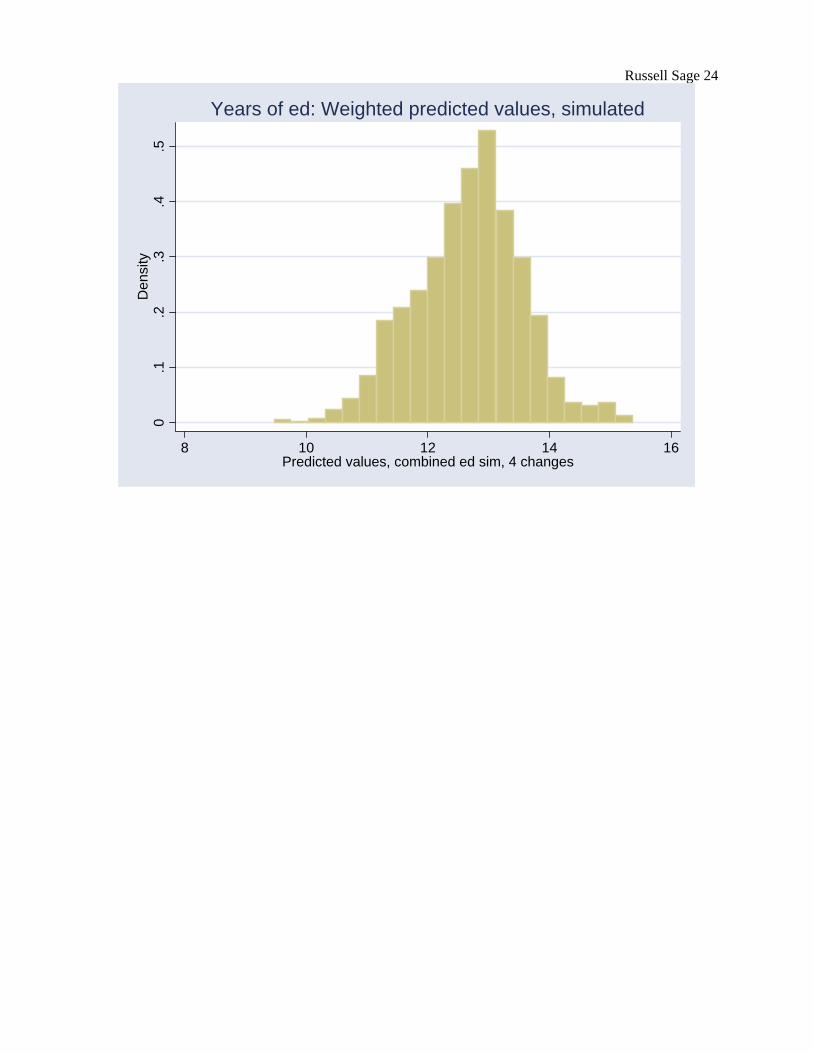
We estimate both the aggregate level of children’s schooling attainment (mean and median years

of schooling) and the inequality of children’s schooling attainment (the standard deviation of years of

schooling). We also estimate the proportion of children who are simulated to not graduate high school and

the proportion not expected to complete 11 years of school, using the adjusted variables of interest. Then,

we compare these medians, standard deviations and proportions with the actual levels recorded in the

data. We present results that are weighted to reflect national levels of attainment for this cohort of

individuals.

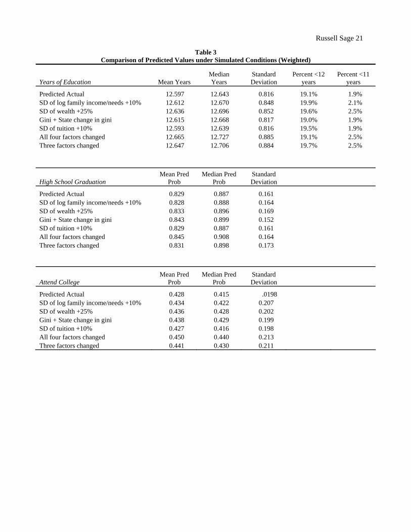
Table 3 shows the predicted values of both outcomes, before and after simulated increases in

inequality. The first row in Table 3 shows the mean, median, and standard deviation of predicted values

of years of schooling based on the estimates in Table 2. The last two columns in this row give the

percentage of individuals with less than 12 years of schooling and the percent below 11 years of

schooling. The next four rows summarize the impact on years of schooling of the simulated increases in

inequality in our four independent variables of interest.

The results in the top of Table 3 show that an increase in inequality of family income or wealth

results in an increase in the inequality of schooling outcomes. Changes in the state gini or tuition, on the

other hand, do not lead to changes in inequality in years of completed schooling. The standard deviation

of years of schooling increases by approximately 4 percent when income or wealth inequality increases.

Further these simulated changes increase the percentages of individuals who have less than a high school

education (less than 12 years) and the percentage that completes less than 11 years of school.

In reality, however, we would never expect an increase in income inequality without an increase

in wealth inequality, and it is impossible to see those changes without a corresponding increase in the gini

index. The best indicators of real changes in the inequality of outcomes, therefore, are the predicted

Russell Sage 14

values when all four factors change. With this scenario, the standard deviation of schooling outcomes

increases even more—by over 8 percent—and there are significant increases in the number of youth not

achieving 11 years of education.20

These numbers are not surprising; they reflect commonly estimated relationships between family

income, wealth, inequality and college tuition and educational outcomes. Importantly, they suggest that

increased inequality in these dimensions increases the disparity in educational attainment among members

of the next generation.

The middle of Table 3 shows the mean, median and standard deviation of the probability of

graduating from high school under different simulated conditions. Not surprisingly, this outcome

indicates a smaller response to simulated increases in family and regional economic inequality. In all

cases, including the base estimate and the simulated estimates, most of the sample is predicted to graduate

from high school. Increases in the inequality of family income and wealth do result in small increases in

the inequality of this outcome as well, although the changes are smaller.21 We conclude that although high

school graduation probabilities are fairly high today in most contexts, increases in family income and

especially wealth inequality would probably result in small increases in inequality for this outcome as

well. When inequality of income, wealth and tuition are jointly increased, the standard deviation increases

by 7.5 percent. The biggest contributor to this increase in inequality is the increase in inequality of wealth.

The last section of Table 3 shows the mean, median and standard deviation of the probability of

attending college for those who graduated from high school. In this case an increase in family income

inequality or wealth inequality is associated with very small changes (around 1 percent) in the probability

20If we instead base our simulations on the model in which we include race interactions (see note 14

above,) we find similar patterns. In these we simulate that the standard deviation would increase by 7 percent among whites when all four changes are simulated (from .848 to .906) while for Blacks it would increase by 9 percent or from .654 to .712. The proportion with less than 12 years of schooling would increase from 17.3 percent (36.9 percent) to 17.6 percent (39.6 percent), respectively, while the proportion simulated to have less than 11 years increases from 2.8 percent (3.9 percent) to 3.3 percent (4.4 percent). (See Appendix Table 2)

21The simulated increase in the state gini coefficients suggests an increase in the mean probability of high school graduation, and a decrease in the variation in this outcome; however, the coefficient on this variable is marginally significant and the conceptual linkage between college costs and high school graduation is less convincing than between these costs and years of schooling.

Russell Sage 15

of attending college when they are considered alone. However, when all four factors changed (or three

factors) change, there is an increase of around 7 percent in the standard deviation or our measure of

inequality of educational outcomes.

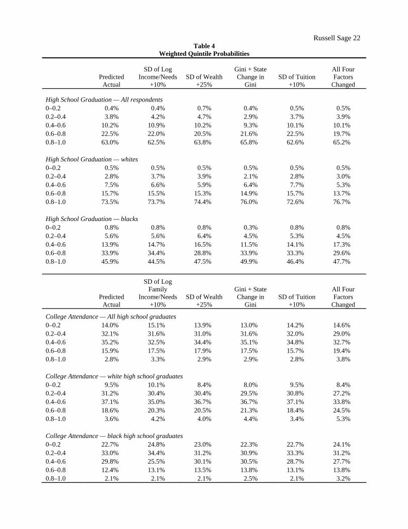
We use several other measures of inequality in an attempt to better understand the nature of the

change in schooling in response to the changes in our indicators of changing income and wealth

inequality (income, wealth, state ginis and state public university tuition.). We report the distribution of

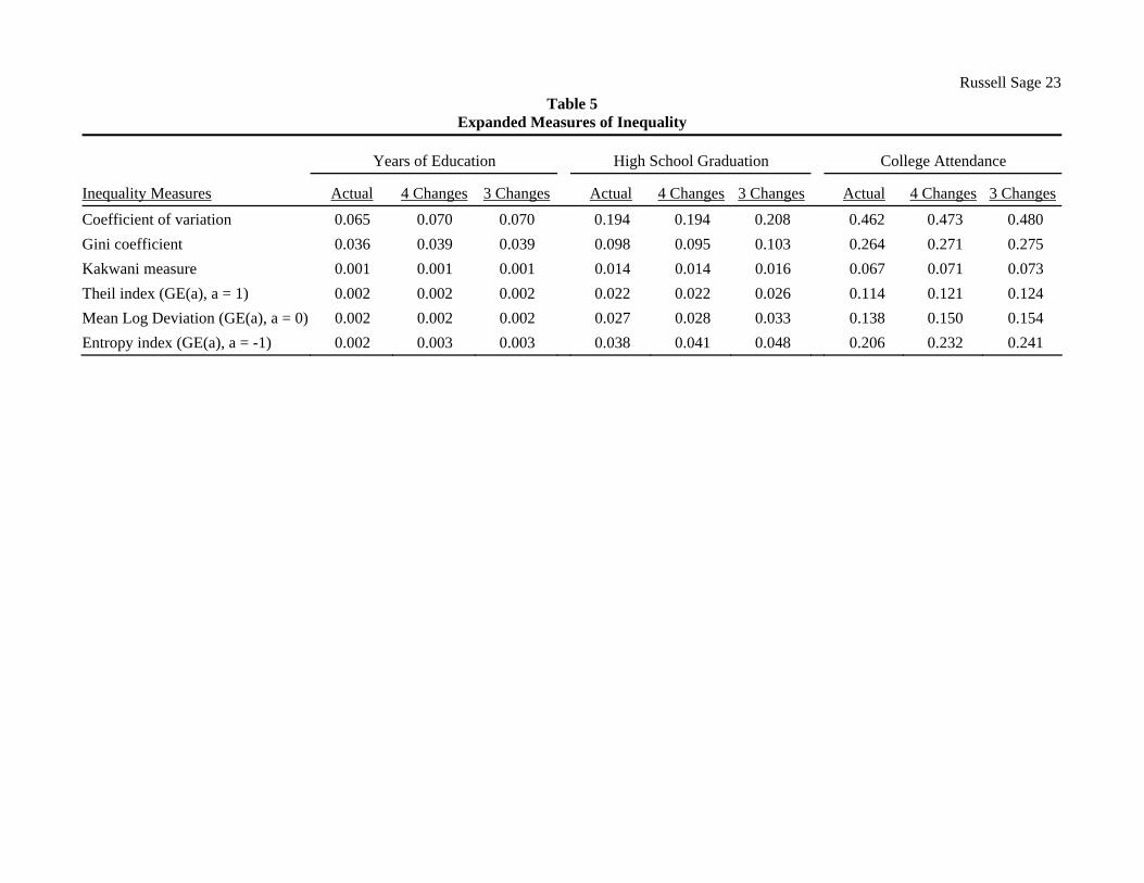
probabilities by quintiles (see table 4), which is descriptive. We report the gini coefficient, and a series of

other summary inequality measures (the coefficient of variation, the Theil index, the Theil entropy

measure, the Theil mean log deviation measure, and the Kakwani index).22 These measures were selected

to reflect a variety of inequality attributes of the distributions. The measures we include rank the

distribution of education outcomes with equal weights above and below the average (gini and Theil

index), weights that values observations farthest from the average most highly (coefficient of variation or

CV and Kakwani), and that weights changes in the lower end of the distribution most highly (Theil mean

log deviation and the Theil entropy index) The results are reported in table 5 using both three changes

(income, wealth and tuition) and four (the three plus changes in the state ginis.)

Turning first to the change in the probability of high school graduation, we find that the Gini

coefficient suggests that the probability of high school graduation has become slightly more equal when

we model the four changes, but slightly more unequal if we consider only the three changes. All of the

other measures show an increase in the inequality in the probability of graduating. Most suggest the

22The gini coefficient is sensitive to changes across the distribution. It meets the criteria of mean independence (double everyone’s income and the value of the index remains the same), symmetry (it does not matter is poor only the number who are poor), independence from sample size, and the so-called Pigou-Dalton transfer sensitivity or inequality is increased when a transfer is made from a poor person to a rich one. It is not decomposable and tests of significant differences must rely on bootstrapping techniques. We also report the three Theil entrophy measures which meet all the above criteria including decomposability. The entrophy measure is most sensitive to changes in the lower end of the distribution while the Theil index is more balanced in giving weight across the distribution and so is closer to the gini in that regard, the mean log deviation is intermediate giving more weight to the lower end but less than the entrophy measure. The coefficient of variation is more sensitive to higher and lower values though it does not meet all of these criteria. The CV is the square root of the variance divided by the mean. A CV of zero indicates no inequality within a distribution; however, its upper limit, in theory, is infinite. The Kakwani index is similar to the Gini, which is 1 minus the area under the Lorenz curve measuring the inequality in the distribution of education (or the probability of achieving a specified level of education), except that the Kakwani index squares the area under the Lorenz curve so that larger values are given greater weight.

Russell Sage 16

increase is small; the exception is the entropy index which places more emphasis on the change for those

closest to the bottom of the distribution; it shows about a nine percent increase in inequality. Overall the

measures suggest a small increase in inequality in the probability of high school graduation due to the

changes in income, wealth, tuition and the state gini coefficient. The results simulating the three changes

(excluding changes in the state ginis) suggest more substantial increases in the inequality of the

probability of completing high school. Again those that emphasize low valued observations show the

largest increase in inequality.

The results for years of education are more consistent. All of the reported measures of inequality

suggest that the distribution of years of education has become more unequal after the observed changes in

inequality of income, wealth, state incomes and public tuition, or for the three changes excluding state

ginis. The gini coefficient increases by about 8 percent in both simulations; the three Theil indices by

about 16–17 percent; and the CV by about 8 percent or by the same percentage as the gini coefficient. The

simulations are remarkably similar for the three and four income/wealth changes. The pattern suggests an

overall increase in inequality including a considerably greater loss of opportunity at the bottom end of the

distribution.

By every measure simulating inequality for all four changes (income wealth, state ginis and

college tuition), inequality is greater for college attendance than for years of schooling or the probability

of graduating high school. All of the inequality measures show increases in inequality in terms of the

probability of attending college in response to the changes we simulate. In this case we find an increase

that varies from about a three percentage increase for the gini coefficient for all four changes to 17

percent for the two Theil indices that emphasize those at the lower end when including only three changes

in income/wealth inequality. All suggest sizeable increases in the inequality of the probability of

attending college due to the changes in income, wealth and tuition that have taken place in the United

States.

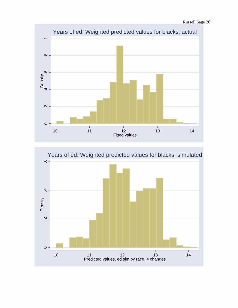
In Appendix Table 2 we present the results for the two racial groups in our sample: whites and

blacks. In all cases we observe the lower levels of education among blacks compared to whites. However,

Russell Sage 17

with few exceptions, the increase in inequality of outcomes is similar for the two groups. The increase in

family income and in family wealth is associated with a substantial increase in inequality of years of

education and the proportion predicted to have less than 11 or 12 years of education. When simulating the

expected change due to an increase in either all 4 or all 3 factors, the standard deviation of each group

increases by about 8.6 percent. However, among non-whites there appears to be a larger difference in the

increase in the standard deviation of years of schooling in response to the simulation of an increase of 25

percent in family wealth (5.6 percent compared to 4 percent.)

Comparing the simulations of mean, median and standard deviation for high school graduates, it

appears that non-whites show a larger expected increase in inequality especially in response to increases

in inequality of family wealth and in response to the changing of the three factors simultaneously (in the

latter case the predicted increase is about 11 percent for non-whites and 6 percent for whites. In the case

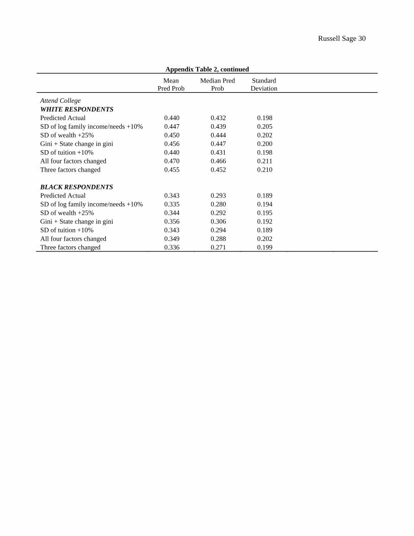
of attending college, the exception to the similar pattern among whites and non-whites is the response to

an increase in inequality in family wealth that appears to decrease inequality among whites while

increasing it somewhat among non-whites.

In viewing these simulations, it is important to keep in mind that while we model actual changes

in income, wealth, public tuition and state ginis we do so in a particular way that may not reflect the

pattern of actual changes.

IV. CONCLUSION

The social science and the policy communities have been concerned for some time about the

possible implications of increases in inequality during the past several years. We know that our society

has experienced increases in inequality in both family income and wealth. We also know that there is

some evidence that individuals and families are becoming increasingly concentrated in either very

affluent or very impoverished areas. The research of Mayer and others suggests that increases in income

inequality as measured at the state level have increased inequality in educational outcomes. Similarly, as

Russell Sage 18

postsecondary education rises in importance, the influence of college tuition levels also gains significance

for understanding educational inequality.

In this paper we pose a related but different question: What may have been the impact of

increases in inequality measured at the family level on educational outcomes in the next generation? Our

results suggest that increases in family income inequality and family wealth inequality have likely

produced an upward influence on the dispersion of educational outcomes. Ceteris paribus, increases in

family economic inequality are associated with increases in inequality in educational attainment in the

next generation. Given the linkage between schooling attainments and labor market success, it seems

likely that increases in inequality in educational attainment will also result in an increase in earnings

inequality. In sum, increases in inequality have important intergenerational effects that we as a society

cannot afford to ignore. If such increases persist across generations, the bottom and top of the education

and income distributions are likely to grow farther and farther apart.

Public policy can be used to alleviate some of the effects of growing inequality on inequality in

educational attainment in the next generation. Compulsory schooling and free public education through

high school creates a threshold of high school graduation below which few people need be. Unfortunately

some people continue to be below that threshold. Efforts to assist low-income students to obtain post-

secondary education also help to alleviate some of the impacts of growing income and wealth inequality.

The large increases in the inequality as captured by those indices that emphasize the lower part of the

distribution seem to call for intervention. It appears that without additional public intervention, the

inequality in schooling will increase sizably, and with it prospects for decreasing inequality in income and

wealth in the future.

Russell Sage 19

Table 1 Unweighted Descriptive Statistics

Obs Mean S.D. Min Max High school graduate 1350 0.73 0.44 0.00 1.00 Attended College 1348 0.29 0.45 0.00 1.00 Years completed education 1348 12.18 1.67 2.00 17.00 African American 1426 0.45 0.50 0.00 1.00 Female 1426 0.47 0.50 0.00 1.00 Average number of siblings 2–15 1423 2.09 1.48 0.00 8.43 At least one parent graduated H.S. 1426 0.61 0.49 0.00 1.00 At least one parent attended college 1426 0.25 0.43 0.00 1.00 Education info missing for both parents 1426 0.08 0.27 0.00 1.00 Log of family income/poverty level, 2–5 1336 0.58 0.64 -2.27 2.79 Log of family income/poverty level, 6–11 1396 0.65 0.68 -1.48 3.38 Log of family income/poverty level, 12–15 1421 0.66 0.76 -1.77 3.59 Proportion years with single parent, 2–15 1414 0.27 0.37 0.00 1.00 Number of moves 2–15 1368 2.80 2.56 0.00 12.00 Head foreign born 1410 0.02 0.15 0.00 1.00 Average county unemployment 2–15 1412 6.61 2.12 1.50 30.67 Percent NH dropouts 2–15 1368 16.83 8.69 0.00 67.29 Percent NH persons low income 2–15 1420 27.80 14.28 2.07 75.30 Log of positive wealth, 1984 1426 6.77 5.03 0.00 16.12 Negative wealth, 1984 1426 0.05 0.22 0.00 1.00 Wealth missing, 1984 1426 0.20 0.40 0.00 1.00 State gini index ages 2–5 1416 0.37 0.03 0.33 0.43 State gini index ages 5–11 1419 0.37 0.02 0.34 0.43 State gini index, ages 12–15 1417 0.38 0.02 0.34 0.44 Tuition & fees per FTE student/1000, Public 85–90 1321 1.59 0.54 0.705 4.78 Public tuition * youngest kids 1321 0.34 0.71 0.00 4.78 Child care costs above $1000, age 2–5 1416 0.15 0.36 0.00 1.00

Russell Sage 20 Table 2

Regression Results

Years of Completed

Schooling High School Graduation

Attend College

OLS Coeff. Logit Coeff. Logit Coeff. African American 0.486*** 0.599*** 0.694*** (0.109) (0.197) (0.202) Female 0.338*** 0.443*** 0.554*** (0.085) (0.155) (0.149) Average number of siblings 2–15 -0.075** -0.057 -0.169** (0.035) (0.059) (0.069) At least one parent grad h.s. 0.381*** 0.764*** -0.007 (0.113) (0.189) (0.217) At least one parent attend college 0.159 0.298 0.196 (0.114) (0.241) (0.185) Education info missing for both parents 0.462** 0.526* 0.604* (0.181) (0.294) (0.346) Family income/poverty level, 2–5, logged 0.384*** 0.616*** 0.384 (0.132) (0.233) (0.252) Family income/poverty level, 6–11, logged -0.168 -0.711** -0.097 (0.161) (0.281) (0.308) Family income/poverty level, 12–15, logged 0.336*** 0.625*** 0.574** (0.118) (0.205) (0.226) Proportion yrs w/single parent 2–15 0.095 -0.078 -0.081 (0.155) (0.267) (0.290) # moves 2–15 -0.057*** -0.071** -0.040 (0.018) (0.030) (0.034) Head foreign born 1.189*** 2.087* 1.114** (0.306) (1.097) (0.505) Average county unemployment 2–15 -0.053** -0.094** -0.011 (0.023) (0.043) (0.039) Percent NH dropouts 2–15 -0.024*** -0.030*** -0.029*** (0.005) (0.010) (0.010) State gini, avg 12–15 0.682 5.076 1.832 (2.621) (4.787) (4.592) Log of positive wealth, 1984 0.050*** 0.100*** 0.043 (0.017) (0.027) (0.036) Negative wealth, 1984 0.194 0.252 -0.021 (0.232) (0.353) (0.504) Wealth missing, 1984 -0.769*** -0.940*** -0.766 (0.196) (0.303) (0.503) Tuition & fees per FTE student, PUBLIC 87 -0.036 0.261 -0.103 (0.091) (0.170) (0.155) Tuition & fees* youngest cohort -0.154** -0.224** -0.050 (0.064) (0.114) (0.117) Child care costs above $1000, 2–5 -0.210* -0.349 -0.040 (0.123) (0.227) (0.213) Constant 11.813*** -1.405 -1.633 (1.102) (2.024) (1.927) Observations 1209 1210 906

Standard errors in parentheses * significant at 10%; ** significant at 5%; *** significant at 1%

Russell Sage 21

Table 3 Comparison of Predicted Values under Simulated Conditions (Weighted)

Years of Education Mean Years Median Years

Standard Deviation

Percent <12 years

Percent <11 years

Predicted Actual 12.597 12.643 0.816 19.1% 1.9% SD of log family income/needs +10% 12.612 12.670 0.848 19.9% 2.1% SD of wealth +25% 12.636 12.696 0.852 19.6% 2.5% Gini + State change in gini 12.615 12.668 0.817 19.0% 1.9% SD of tuition +10% 12.593 12.639 0.816 19.5% 1.9% All four factors changed 12.665 12.727 0.885 19.1% 2.5% Three factors changed 12.647 12.706 0.884 19.7% 2.5%

High School Graduation Mean Pred

Prob Median Pred

Prob Standard Deviation

Predicted Actual 0.829 0.887 0.161 SD of log family income/needs +10% 0.828 0.888 0.164 SD of wealth +25% 0.833 0.896 0.169 Gini + State change in gini 0.843 0.899 0.152 SD of tuition +10% 0.829 0.887 0.161 All four factors changed 0.845 0.908 0.164 Three factors changed 0.831 0.898 0.173

Attend College Mean Pred

Prob Median Pred

Prob Standard Deviation

Predicted Actual 0.428 0.415 .0198 SD of log family income/needs +10% 0.434 0.422 0.207 SD of wealth +25% 0.436 0.428 0.202 Gini + State change in gini 0.438 0.429 0.199 SD of tuition +10% 0.427 0.416 0.198 All four factors changed 0.450 0.440 0.213 Three factors changed 0.441 0.430 0.211

Russell Sage 22 Table 4

Weighted Quintile Probabilities

Predicted

Actual

SD of Log Income/Needs

+10% SD of Wealth

+25%

Gini + State Change in

Gini SD of Tuition

+10%

All Four Factors

Changed

High School Graduation — All respondents 0–0.2 0.4% 0.4% 0.7% 0.4% 0.5% 0.5% 0.2–0.4 3.8% 4.2% 4.7% 2.9% 3.7% 3.9% 0.4–0.6 10.2% 10.9% 10.2% 9.3% 10.1% 10.1% 0.6–0.8 22.5% 22.0% 20.5% 21.6% 22.5% 19.7% 0.8–1.0 63.0% 62.5% 63.8% 65.8% 62.6% 65.2% High School Graduation — whites 0–0.2 0.5% 0.5% 0.5% 0.5% 0.5% 0.5% 0.2–0.4 2.8% 3.7% 3.9% 2.1% 2.8% 3.0% 0.4–0.6 7.5% 6.6% 5.9% 6.4% 7.7% 5.3% 0.6–0.8 15.7% 15.5% 15.3% 14.9% 15.7% 13.7% 0.8–1.0 73.5% 73.7% 74.4% 76.0% 72.6% 76.7% High School Graduation — blacks 0–0.2 0.8% 0.8% 0.8% 0.3% 0.8% 0.8% 0.2–0.4 5.6% 5.6% 6.4% 4.5% 5.3% 4.5% 0.4–0.6 13.9% 14.7% 16.5% 11.5% 14.1% 17.3% 0.6–0.8 33.9% 34.4% 28.8% 33.9% 33.3% 29.6% 0.8–1.0 45.9% 44.5% 47.5% 49.9% 46.4% 47.7%

Predicted

Actual

SD of Log Family

Income/Needs +10%

SD of Wealth +25%

Gini + State Change in

Gini SD of Tuition

+10%

All Four Factors

Changed

College Attendance — All high school graduates 0–0.2 14.0% 15.1% 13.9% 13.0% 14.2% 14.6% 0.2–0.4 32.1% 31.6% 31.0% 31.6% 32.0% 29.0% 0.4–0.6 35.2% 32.5% 34.4% 35.1% 34.8% 32.7% 0.6–0.8 15.9% 17.5% 17.9% 17.5% 15.7% 19.4% 0.8–1.0 2.8% 3.3% 2.9% 2.9% 2.8% 3.8% College Attendance — white high school graduates 0–0.2 9.5% 10.1% 8.4% 8.0% 9.5% 8.4% 0.2–0.4 31.2% 30.4% 30.4% 29.5% 30.8% 27.2% 0.4–0.6 37.1% 35.0% 36.7% 36.7% 37.1% 33.8% 0.6–0.8 18.6% 20.3% 20.5% 21.3% 18.4% 24.5% 0.8–1.0 3.6% 4.2% 4.0% 4.4% 3.4% 5.3% College Attendance — black high school graduates 0–0.2 22.7% 24.8% 23.0% 22.3% 22.7% 24.1% 0.2–0.4 33.0% 34.4% 31.2% 30.9% 33.3% 31.2% 0.4–0.6 29.8% 25.5% 30.1% 30.5% 28.7% 27.7% 0.6–0.8 12.4% 13.1% 13.5% 13.8% 13.1% 13.8% 0.8–1.0 2.1% 2.1% 2.1% 2.5% 2.1% 3.2%

Russell Sage 23 Table 5

Expanded Measures of Inequality

Years of Education High School Graduation College Attendance

Inequality Measures Actual 4 Changes 3 Changes Actual 4 Changes 3 Changes Actual 4 Changes 3 Changes

Coefficient of variation 0.065 0.070 0.070 0.194 0.194 0.208 0.462 0.473 0.480 Gini coefficient 0.036 0.039 0.039 0.098 0.095 0.103 0.264 0.271 0.275 Kakwani measure 0.001 0.001 0.001 0.014 0.014 0.016 0.067 0.071 0.073 Theil index (GE(a), a = 1) 0.002 0.002 0.002 0.022 0.022 0.026 0.114 0.121 0.124 Mean Log Deviation (GE(a), a = 0) 0.002 0.002 0.002 0.027 0.028 0.033 0.138 0.150 0.154 Entropy index (GE(a), a = -1) 0.002 0.003 0.003 0.038 0.041 0.048 0.206 0.232 0.241

Russell Sage 24

0.1

.2.3

.4.5

Den

sity

8 10 12 14 16Predicted values, combined ed sim, 4 changes

Years of ed: Weighted predicted values, simulated

Russell Sage 25

0.2

.4.6

Den

sity

10 11 12 13 14 15Fitted values

Years of ed: Weighted predicted values for whites, actual

0.1

.2.3

.4.5

Den

sity

8 10 12 14 16Predicted values, ed sim by race, 4 changes

Years of ed: Weighted predicted values for whites, simulated

Russell Sage 26

0.2

.4.6

.81

Den

sity

10 11 12 13 14Fitted values

Years of ed: Weighted predicted values for blacks, actual

0.2

.4.6

Den

sity

10 11 12 13 14Predicted values, ed sim by race, 4 changes

Years of ed: Weighted predicted values for blacks, simulated

Russell Sage 27 Appendix Table 1

Regression Results: Interactions with Race

Years of Completed Schooling

High School Graduation

Attend College

OLS Coeff. Logit Coeff. Logit Coeff.

African American 0.809** 1.107* 0.573 (0.360) (0.646) (0.668) Female 0.322*** 0.411*** 0.570*** (0.085) (0.157) (0.151) Average number of siblings 2–15 -0.083** -0.065 -0.172** (0.035) (0.060) (0.070) At least one parent grad h.s. 0.623*** 1.106*** 0.246 (0.163) (0.271) (0.332) At least one parent attend college 0.163 0.365 0.185 (0.136) (0.302) (0.218) Education info missing for both parents 0.336 -0.049 -0.011 (0.428) (0.689) (0.982) Family income/poverty level, 2–5, logged 0.307 0.602 0.306 (0.192) (0.374) (0.343) Family income/poverty level, 6–11, logged -0.457** -1.021** -0.607 (0.225) (0.435) (0.422) Family income/poverty level, 12–15, logged 0.585*** 0.765*** 0.906*** (0.154) (0.294) (0.298) Proportion yrs w/single parent 2–15 0.139 0.003 0.086 (0.159) (0.273) (0.300) # moves 2–15 -0.058*** -0.074** -0.044 (0.018) (0.030) (0.035) Head foreign born 1.184*** 2.055* 1.104** (0.307) (1.104) (0.503) Average county unemployment 2–15 -0.042 -0.059 -0.010 (0.030) (0.062) (0.051) Percent NH dropouts 2–15 -0.024*** -0.031*** -0.032*** (0.006) (0.010) (0.011) State gini, avg 12–15 1.303 6.019 2.856 (2.629) (4.801) (4.654) Log of positive wealth, 1984 0.049*** 0.092*** 0.044 (0.017) (0.028) (0.037) Negative wealth, 1984 0.172 0.155 -0.033 (0.234) (0.357) (0.514) Wealth missing, 1984 -0.795*** -1.048*** -0.780 (0.199) (0.313) (0.516) Tuition & fees per FTE student, PUBLIC 87 -0.049 0.235 -0.134 (0.091) (0.171) (0.157) Tuition & fees* youngest cohort -0.177** -0.210 0.017 (0.084) (0.158) (0.148) Child care costs above $1000, 2–5 -0.334** -0.556* -0.290 (0.153) (0.294) (0.263)

(table continues)

Russell Sage 28

Appendix Table 1, continued

Years of Completed Schooling

High School Graduation

Attend College

OLS Coeff. Logit Coeff. Logit Coeff.

INTERACTIONS Black*parent completed HS -0.467** -0.683* -0.523 (0.227) (0.378) (0.451) Black*parent attended college -0.104 -0.285 -0.007 (0.262) (0.517) (0.442) Black*parent ed missing 0.071 0.618 0.556 (0.471) (0.764) (1.043) Black*family income/poverty, logged, 2–5 0.134 0.016 0.142 (0.260) (0.474) (0.496) Black*family income/poverty, logged, 6–11 0.635** 0.612 1.198* (0.317) (0.563) (0.618) Black*family income/poverty, logged, 12–15 -0.556** -0.243 -0.709 (0.230) (0.405) (0.452) Black*unemployment, 2–15 -0.033 -0.068 0.002 (0.046) (0.085) (0.080) Black*Tuition and fees, youngest cohort 0.054 -0.027 -0.217 (0.129) (0.224) (0.246) Black*Child care costs above $1000, 2–5 0.325 0.530 0.659 (0.255) (0.466) (0.441) Constant 11.502*** -1.854 -1.911 (1.105) (2.047) (1.943) Observations 1209 1210 906

Standard errors in parentheses * significant at 10%; ** significant at 5%; *** significant at 1%

Russell Sage 29

Appendix Table 2 Racial Comparison of Predicted Values under Simulated Conditions (Weighted)

Mean Years Median Years Standard Deviation

Percent <12 years

Percent <11 years

Years of Education WHITE RESPONDENTS Predicted Actual 12.686 12.750 0.848 17.3% 2.8% SD of log family income/needs +10% 12.704 12.758 0.876 17.2% 3.0% SD of wealth +25% 12.731 12.794 0.876 17.5% 3.1% Gini + State change in gini 12.720 12.784 0.850 17.0% 2.6% SD of tuition +10% 12.683 12.747 0.850 17.4% 2.9% All four factors changed 12.781 12.843 0.908 17.3% 2.9% Three factors changed 12.746 12.812 0.906 17.6% 3.3% BLACK RESPONDENTS Predicted Actual 12.141 12.076 0.654 36.9% 3.9% SD of log family income/needs +10% 12.121 12.043 0.665 39.2% 3.9% SD of wealth +25% 12.135 12.118 0.699 38.6% 4.5% Gini + State change in gini 12.172 12.122 0.650 36.2% 3.2% SD of tuition +10% 12.141 12.084 0.654 37.1% 4.2% All four factors changed 12.146 12.108 0.708 38.7% 4.4% Three factors changed 12.115 12.080 0.712 39.6% 4.4%

Mean

Pred Prob Median Pred

Prob Standard Deviation

High School Graduation WHITE RESPONDENTS Predicted Actual 0.848 0.910 0.160 SD of log family income/needs +10% 0.847 0.909 0.163 SD of wealth +25% 0.853 0.917 0.164 Gini + State change in gini 0.862 0.920 0.151 SD of tuition +10% 0.847 0.909 0.161 All four factors changed 0.866 0.929 0.158 Three factors changed 0.852 0.917 0.167 BLACK RESPONDENTS Predicted Actual 0.730 0.775 0.174 SD of log family income/needs +10% 0.724 0.769 0.176 SD of wealth +25% 0.722 0.780 0.191 Gini + State change in gini 0.755 0.790 0.163 SD of tuition +10% 0.730 0.773 0.174 All four factors changed 0.741 0.790 0.181 Three factors changed 0.716 0.773 0.193

(table continues)

Russell Sage 30

Appendix Table 2, continued

Mean

Pred Prob Median Pred

Prob Standard Deviation

Attend College WHITE RESPONDENTS Predicted Actual 0.440 0.432 0.198 SD of log family income/needs +10% 0.447 0.439 0.205 SD of wealth +25% 0.450 0.444 0.202 Gini + State change in gini 0.456 0.447 0.200 SD of tuition +10% 0.440 0.431 0.198 All four factors changed 0.470 0.466 0.211 Three factors changed 0.455 0.452 0.210 BLACK RESPONDENTS Predicted Actual 0.343 0.293 0.189 SD of log family income/needs +10% 0.335 0.280 0.194 SD of wealth +25% 0.344 0.292 0.195 Gini + State change in gini 0.356 0.306 0.192 SD of tuition +10% 0.343 0.294 0.189 All four factors changed 0.349 0.288 0.202 Three factors changed 0.336 0.271 0.199

Russell Sage 31 References Adler, N. E., T. Boyce, M. A. Chesney, S. Cohen, S. Folkman, R. L. Kahn, and S. L. Syme. 1994.

“Socioeconomic Status and Health: The Challenge of the Gradient.” American Psychologist 49: 15–24.

Becketti, Sean, William Gould, Lee Lillard, and Finis Welch. 1988. “The PSID after Fourteen Years: An Evaluation.” Journal of Labor Economics 6(4, September): 472–492.

Diez-Roux A. V., F. J. Nieto, C. Muntaner, H. A. Tyroler, G. W. Comstock, E. Shahar, L. S. Cooper, R. L. Watson, and M. Szklo. 1997. “Neighborhood Environments and Coronary Heart Disease: A Multilevel Analysis.” American Journal of Epidemiology 146 (1): 48–63.

Fitzgerald, John, Peter Gottschalk, and Robert Moffitt. 1998. “An Analysis of Sample Attrition in Panel Data: The Michigan Panel Study of Income Dynamics.” Journal of Human Resources 33(2): 251–299.

Haveman, Robert, and Barbara Wolfe. 1994. Succeeding Generations: On the Effects of Investments in Children. New York: Russell Sage Foundation.

—————. 1995. “The Determinants of Children’s Attainments: A Review of Methods and Findings.” Journal of Economic Literature 33(4): 1829–1878.

Haveman, Robert, Barbara Wolfe, and Kathryn Wilson. 1997. “Childhood Poverty and Adolescent Schooling and Fertility Outcomes: Reduced-Form and Structural Estimates.” In Consequences of Growing Up Poor, edited by Greg J. Duncan and Jeanne Brooks-Gunn. New York: Russell Sage Foundation.

Haveman, Robert, Gary Sandefur, Barbara Wolfe and Andrea Voyer. 2001. “Inequality of Family and Community Characteristics in Relation to Children's Attainments.” Russell Sage Foundation. http://www.russellsage.org/programs/proj_reviews/social-inequality.htm

Jargowsky, Paul A. 1997. Poverty and Place: Ghettos, Barrios, and the American City. New York: Russell Sage Foundation.

Kawachi, Ichiro, and Bruce P. Kennedy. 1997. “The Relationship of Income Inequality to Mortality: Does the Choice of Indicator Matter?” Social Science and Medicine 45: 1121–1127

Lillard, Lee A., and Constantijn W. A. Panis. 1994. “Attrition from the PSID: Household Income, Marital Status, and Mortality.” Santa Monica, CA: Rand Corporation.

Marmot, M. G., G. D. Smith, S. Stansfeld, C. Patel, F. North, J. Head, I. White, E. Brunner, and A. Feeney. 1991. “Health Inequalities among British Civil Servants: The Whitehall II Study.” Lancet 337: 1387–1393.

Massey, Douglas S. 1996. “The Age of Extremes: Concentrated Affluence and Poverty in the Twenty-First Century.” Demography 33(4): 395–412.

Mayer, Susan. 2001. “How Did the Increase in Economic Inequality between 1970 and 1990 Affect Children’s Educational Attainment?” American Journal of Sociology 107(1): 1–32.

McLanahan, Sara, and Gary Sandefur. 1994. Growing Up with A Single Parent: What Hurts? What Helps? Cambridge: Harvard University Press.

Russell Sage 32 Ricketts, Erol R. and Isabel V. Sawhill 1988. “Defining and Measuring the Underclass,”

Journal of Policy Analysis and Management, 7, pp. 316-325.