What are plausible values and why are they useful? · PDF fileWhat are plausible values and...

9

What are plausible values and why are they useful? matthias von DavierEducational Testing Service, Princeton, New Jersey, United States

eugenio GonzalezEducational Testing Service, Princeton, New Jersey, United States

Robert J. mislevyUniversity of Maryland, College Park, Maryland, United States

This paper shows some of the adverse effects that can occur when plausible values are not used or are used incorrectly during analysis of large-scale survey data. To ensure that the uncertainty associated with measures of skills in large-scale surveys is properly taken into account, researchers need to follow the procedures outlined in the article and in more detail in, for example, Little and Rubin (1987) and Schafer (1997). There is no need to rely on computational shortcuts by averaging plausible values before calculations: analytical shortcuts such as averaging plausible values produce biased estimates and should be discouraged. All analyses using survey assessment results need not only use the data as provided by the different assessment organizations but also adhere to the appropriate procedures described in this article and the included references, as well as in the guides provided for users of international survey assessment databases.

10

IERI MONOGRAPH SERIES: ISSUES AND METHODOLOGIES IN LARGE-SCALE ASSESSMENTS

INTRoDuCTIoN

The use of large-scale assessment data to describe what students know and can do has increased, as has the extent to which this information is used to describe group performance and develop educational interventions and policy. International large-scale assessments administer large numbers of items in limited time to representative samples of students, and provide comparable information about student skills and knowledge in content domains such as reading, mathematics, and science. The goal of large-scale educational survey assessments is to collect data on skills assessed in representative samples of student or adult populations. The data are used to describe groups within a population of interest with respect to broadly defined areas of school- or work-relevant skills. They are not used to assign individual test scores to test-takers or to employ scores for individual decision-making.

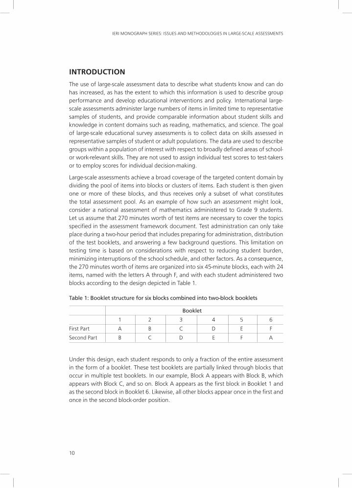
Large-scale assessments achieve a broad coverage of the targeted content domain by dividing the pool of items into blocks or clusters of items. Each student is then given one or more of these blocks, and thus receives only a subset of what constitutes the total assessment pool. As an example of how such an assessment might look, consider a national assessment of mathematics administered to Grade 9 students. Let us assume that 270 minutes worth of test items are necessary to cover the topics specified in the assessment framework document. Test administration can only take place during a two-hour period that includes preparing for administration, distribution of the test booklets, and answering a few background questions. This limitation on testing time is based on considerations with respect to reducing student burden, minimizing interruptions of the school schedule, and other factors. As a consequence, the 270 minutes worth of items are organized into six 45-minute blocks, each with 24 items, named with the letters A through F, and with each student administered two blocks according to the design depicted in Table 1.

Table 1: Booklet structure for six blocks combined into two-block booklets

Booklet

1 2 3 4 5 6

First Part A B C D E F

Second Part B C D E F A

Under this design, each student responds to only a fraction of the entire assessment in the form of a booklet. These test booklets are partially linked through blocks that occur in multiple test booklets. In our example, Block A appears with Block B, which appears with Block C, and so on. Block A appears as the first block in Booklet 1 and as the second block in Booklet 6. Likewise, all other blocks appear once in the first and once in the second block-order position.

11

WHAT ARE PLAUSIBLE VALUES AND WHY ARE THEY USEFUL?

The relatively small number of items per block and the relatively small number of blocks per test booklet mean that the accuracy of measurement at the individual level of these assessments is considerably lower than is the level of accuracy common for individual tests used for diagnosis, tracking, and/or admission purposes. In tests for individual reporting, the number of items administered is considerably more than the number contained in a typical booklet in a large-scale survey assessment.

Because students are measured with only a subset of the total item pool, the measurement of individual proficiency is achieved with a substantial amount of measurement error. Traditional approaches to estimating individual proficiency, such as marginal maximum likelihood (MML) and expected-a-posteriori (EAP) estimates, are point estimates optimal for individual students, not for group-level estimation. These approaches consequently result in biased estimates of group-level results, as we show through examples later in this article.

One way of taking the uncertainty associated with the estimates into account, and of obtaining unbiased group-level estimates, is to use multiple values representing the likely distribution of a student’s proficiency. These so-called plausible values provide us with a database that allows unbiased estimation of the plausible range and the location of proficiency for groups of students. Plausible values are based on student responses to the subset of items they receive, as well as on other relevant and available background information (Mislevy, 1991). Plausible values can be viewed as a set of special quantities generated using a technique called multiple imputations. Plausible values are not individual scores in the traditional sense, and should therefore not be analyzed as multiple indicators of the same score or latent variable (Mislevy, 1993).

In this article, we use simulated data to show and explain, in a non-formal way, the advantages of using plausible values over using traditional point estimates of individual proficiency. We do this by analyzing simulated response data under different conditions, using different estimation methods, and then comparing the results. We finish by summarizing how researchers need to analyze the statistics they obtain when using plausible values so that they can derive unbiased estimates of the quantities of interest.

We have organized this article as follows: the next section presents an illustrative example based on a small sample and an area of human behavior where the relationship between observed variables and the quantity of interest is direct. Our aim in this section is to introduce some important concepts at a basic, non-technical level. These concepts form the basis of statistical tools utilized in data analysis for large-scale survey assessments. We then introduce another example that takes the concepts developed in the first example to the next level. This second example is a much more realistic one: the design is similar to the one above, but it remains compact enough to allow us to discuss the central concepts in a way that focuses on the main ideas.

12


A SImPle exAmPle

Assume we want to predict the score of a basketball free-throw contest,1 and assume we have students from two different schools. Students from School A tend to succeed, on average, on 50% of the free-throw trials, and the success rates across students is normally distributed. Students from School B tend to succeed, on average, on 70% of the free-throw trials, and the success rate across students is also normally distributed. Let us now assume that within each school the standard deviation of a student’s success rate in free throws is 10%. Thus, only a few students in School A are likely to have a “true” free-throw success rate as high as 70%, and only a few of the students from School B are likely to have a free-throw success rate as low as 50%.

We want to come up with a good estimate of a student’s “true” free-throw success rate based on a limited number of observations and our knowledge of the school she attends. Note that we can only observe the trials of a student selected for the tryouts, and we can observe the school the student belongs to (we can ask her). The “true” success rate of 50% cannot be “seen,” and a “true” rate of 50% means that the student does not have to succeed at a rate of 50% in all cases; it simply means that the student with this success rate should succeed in 50% of throws over the long run, and that with each single shot, the student stands a chance of succeeding or failing.

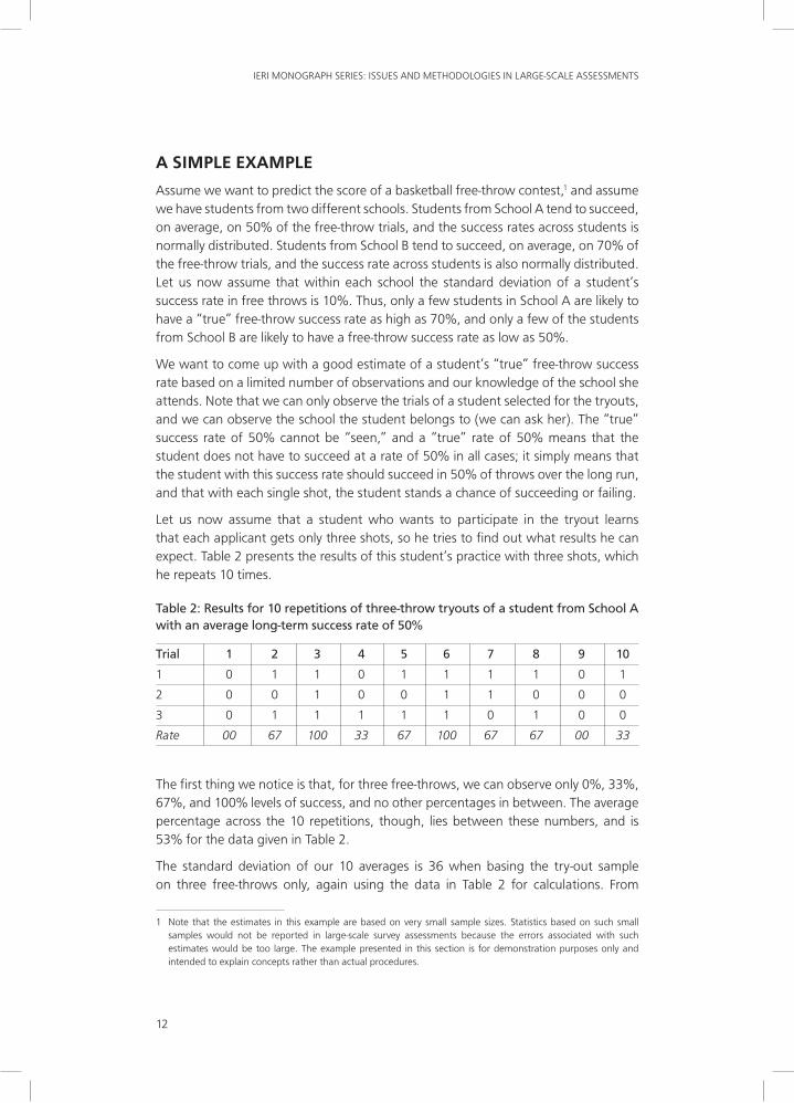
Let us now assume that a student who wants to participate in the tryout learns that each applicant gets only three shots, so he tries to find out what results he can expect. Table 2 presents the results of this student’s practice with three shots, which he repeats 10 times.

Table 2: Results for 10 repetitions of three-throw tryouts of a student from School A with an average long-term success rate of 50%

Trial 1 2 3 4 5 6 7 8 9 10

1 0 1 1 0 1 1 1 1 0 1

2 0 0 1 0 0 1 1 0 0 0

3 0 1 1 1 1 1 0 1 0 0

Rate 00 67 100 33 67 100 67 67 00 33

The first thing we notice is that, for three free-throws, we can observe only 0%, 33%, 67%, and 100% levels of success, and no other percentages in between. The average percentage across the 10 repetitions, though, lies between these numbers, and is 53% for the data given in Table 2.

The standard deviation of our 10 averages is 36 when basing the try-out sample on three free-throws only, again using the data in Table 2 for calculations. From

1 Note that the estimates in this example are based on very small sample sizes. Statistics based on such small samples would not be reported in large-scale survey assessments because the errors associated with such estimates would be too large. The example presented in this section is for demonstration purposes only and intended to explain concepts rather than actual procedures.

13


inspection of this table, we also see that this student would be quite successful in 6 out of 10 cases and produce a success rate of either 100% or 67%. However, there are also two cases with 0% success. Obviously, three throws is a small number from which to accurately estimate the success rate of a player. What happens when the number of throws is increased by a factor of four? Table 3 contains the data for a student with the same actual long-term success rate (50% success rate), who throws 10 repeats of 12 trials each.

Table 3: Results for 10 repetitions of 12-throw tryouts of a student from School A with a long-term success rate of 50%

Trial 1 2 3 4 5 6 7 8 9 10

1 1 0 1 1 0 0 1 0 1 0

2 0 0 0 1 1 0 0 1 1 0

3 1 1 0 1 0 1 0 0 1 1

4 0 1 1 0 1 0 0 1 0 1

5 1 1 1 0 1 0 0 1 0 0

6 0 0 0 1 0 1 1 1 0 0

7 0 1 0 1 1 0 0 0 0 1

8 1 0 1 1 0 0 1 1 1 1

9 1 1 0 1 1 1 1 0 1 0

10 1 0 1 1 1 1 0 1 0 0

11 1 0 1 1 0 1 0 0 0 0

12 0 0 1 1 1 0 1 0 0 1

Rate 58 42 58 83 58 42 42 50 42 42

The 10 averages of 12 trials appear in the last row of Table 3. Notice that there are no cases where all trials were successful (100%) or unsuccessful (0%). The largest success rate in this sample is 83% (repeated trial number 4); the smallest success rate is 42% in the repeated trials 2, 6, 7, 9, and 10. The average success rate of these 12 trials is 52%, and the standard deviation of these averages over 12 trials is 13.5. Note that this is still not exactly 50%, even though this player threw 120 times. This outcome is not an error, but is due to the fact that the actual results of a limited number of trials generally vary somewhat from the long-term expected success rate. Some trials will be slightly below the expected value; some will be slightly above.

We can determine the theoretical standard deviation of the averages mathematically in this simple experiment. The standard deviation of a single trial is 50 in this case, and this number needs to be divided by the square root of the number of trials, which gives us a theoretical standard deviation of the average percentage, that is, the standard error (s. e.) of the estimate of average percentage of success. For a three-throw tryout, the standard deviation of the percentage is 28.87; for the 12-throw trials, it is 14.43. Intuitively, these differences in standard deviations of averages make

14


considerable sense in that more trials per tryout seem to lead to more consistent results.

Unfortunately, this approach to obtaining higher accuracy and reducing uncertainty about the estimate seems to be a rather inefficient one. For a target of a standard error of 5%, we would need 100 free-throws per tryout; a standard error of 1% would require 2,500 throws.

using What We Know about the StudentWhile it would be good to use other students’ tryout throws from the same school as evidence of what we could expect if a student from this school comes to a tryout, how much can we gain from this type of information? Given our knowledge about student averages, and their variability, relative to the long-term success rates from the different schools, we might be able to “stabilize” or “improve” what we know if we could see a very small number of trial free-throws.

What, then, would be our best guess of a student’s success rates on the free throws if we had not seen this student perform any free throws but knew which school he was attending? Our guess would be that this student would have a success rate of 70% if he came from School B. And if he were from School A, his success rate would be 50%, right? So what would we guess if this student threw once and succeeded, and is from School A? Still 50%, or would we guess 100% based on a single trial, or somewhere in between? When we have only a very limited number of observations, it is hard to judge how a player will perform in the long run. In such instances, including information on additional variables, for example, the school the student comes from, can help.

Note that we may not do the right thing for an individual student because we can get lucky in terms of finding a student from School A who has an actual long-term success performance of 70%. We can also find students from School B who have an actual long-term success rate of only 50%. However, this situation changes drastically if we compare groups of students or selections involving multiple students (as in teams, for example).

Group-level ConsiderationsThe person putting together a team and the individual player chosen (or not) as part of that team operate from different perspectives. The person who selects multiple players for a team is interested mostly in how that set of players will perform on average, and how much variability this team will show in terms of performance. The individual player, however, wants his or her actual performance reflected in the most accurate terms.

As a continuation of the tryout example, let us assume that we are in the process of selecting a bunch of new players from the two Schools—A and B. How should we proceed in that case? Let us say we have observed the actual performance on 10 trials for 20 players from each of the two schools. Figure 1 shows a distribution of observed scores generated based on the information we know about the schools and

15


the number of successful free-throws for the two groups. Also shown in the graph in parentheses are the numbers we are interested in but cannot directly see: the actual long-term success rates of each of the students next to their actual score based on the 10 throws. As an example of how to read the graph, Score 4 is observed in two cases in School A and two cases in School B. The students from A who scored 4 have an actual long-run success rate of 39% and 53%, whereas the students from School B with Score 4 have success rates in the long-run of 71% and 43%. Also note that no student from School A scored higher than 8, and no student from School B scored lower than 4.

Figure 1: Distribution of 20 students from each school scoring on 10 free-throws in a tryout for a new team

School A: E=50%, S=10% Score School B: E=70%, S=10%

-/- 0 -/-

-/- 1 -/-

(43%) (33%) 2 -/-

(39%) (58%) 3 -/-

(39%) (53%) 4 (71%) (43%)

(56%) (47%) (43%) (54%) 5 (58%) (55%) (62%) (67%)

(39%) (64%) (54%) (56%) (49%) 6 (70%) (64%) (62%) (70%)

(51%) (49%) (67%) 7 (66%) (67%) (65%) (85%)

(53%) (69%) 8 (65%) (68%) (71%)

-/- 9 (72%) (84%)

-/- 10 (73%)

What is particularly interesting about Figure 1 is the fact that students with rather different “true” success rates get the same observed score on the 10 trials, and that the average “true” success rate by school is also different for the same score level. For example, the group of students with Score 6 has an average “true” success rate of 52.4% (1/5*(39+64+54+56+49)) for School A, and an average of 66.5% (¼*(70+64+62+70)) for students from School B. While readers might think these results are fabricated to make a point,2 these numbers are indeed based on data generated using random draws calculated with a spreadsheet fed with only the basic long-term success rates determined for Schools A and B. We later show how the same phenomenon is observed when we use simulated student response data from an assessment.

Let us now look at the same data from a different perspective. Table 4 gives the means of the “true” success rates of the (admittedly small) groups of students in the percentage metric. It also gives the observed score expressed as a percentage, as well

2 We did not fabricate the values in Figure 1 but obtained them by using a spreadsheet and available statistical functions that allowed us to conduct random draws from a uniform distribution, a function that allows calculation of inverse normal function values, and a Boolean logic function.

16


as the difference between the two. In Table 4, we observe, as we move away from the school average “true” success rate, larger differences between the observed score and the average “true” score of those who obtained it.

Table 4: Observed scores expressed as percentages on 10 trials, average “true” success rates in the score groups by school, and differences between observed scores and averages

Score Mean A Difference A Mean B Difference B

20 38.0 -18.0 -/- -/-

30 48.5 -18.5 -/- -/-

40 46.0 - 6.0 57.0 -17.0

50 50.0 0.0 60.5 -10.5

60 52.4 +7.6 66.5 - 6.5

70 55.7 +14.3 70.8 +0.8

80 61.0 +19.0 68.0 +12.0

90 -/- -/- 78.0 +12.0

100 -/- -/- 73.0 +27.0

These differences seem to be centered on the average skill we identified for the two schools. The smallest difference between the observed score and the average “true” skill of students from School A is found for score 50 (which is also the average percentage of success for School A). The smallest difference between the observed scores and the average “true” skill of students from School B is found at score level 70 (which is the average success rate overall for students in School B).

Given these observations, we would substantially misjudge the situation if we were to state that students from School A with a score of 60 (6/10 successful throws x 100) have the same average success rate compared to students from School B with a score of 60. In our example, the average success rate based on the long-term rates for students with this score is 52.4% for students from School A and 66.5% for students from School B. (We will show this effect again later with our simulated assessment data from a much larger sample.) For the person forming a new team, the best decision would be to select students from School B at a higher rate than students from School A, even if those students have the same observed score, because the long-term success rate of students seems to be higher for students in School B than for those in School A.

There is a way of taking into account the fact that we know, from previous trials, how students from these different school teams perform, on average, and how their performance varies. Table 5 provides an example of how this might look. Note that, for only one throw, we would remain very close to the school-based long-term averages as our guess for the student’s expected long-term success rate. Because we

17


do not know much after seeing just one successful throw, all we can do is estimate that a student who throws once and succeeds will have a expected long-term success rate of 51.92% if she is from School A and an estimated long-term success rate of 71.36% if she is from School B.

Table 5: Average long-term success rate used to derive expected success rates given the successes on a number of throws, Schools A and B

A B A B A B A B

Throws 1 1 10 10 100 100 500 500

0.00 48.08 66.82 35.71 47.42 10.00 12.15 2.38 2.82

10.00 -/- -/- 38.57 50.65 18.00 20.41 11.90 12.42

20.00 -/- -/- 41.43 53.87 26.00 28.68 21.43 22.02

30.00 -/- -/- 44.29 57.10 34.00 36.94 30.95 31.61

40.00 -/- -/- 47.14 60.32 42.00 45.21 40.48 41.21

50.00 -/- -/- 50.00 63.55 50.00 53.47 50.00 50.81

60.00 -/- -/- 52.86 66.77 58.00 61.74 59.52 60.40

70.00 -/- -/- 55.71 70.00 66.00 70.00 69.05 70.00

80.00 -/- -/- 58.57 73.23 74.00 78.26 78.57 79.60

90.00 -/- -/- 61.43 76.45 82.00 86.53 88.10 89.19

100.00 51.92 71.36 64.29 79.68 90.00 94.79 97.62 98.79

Note: Values given are for one throw, 10 throws, 100 throws, 500 throws.

This situation changes markedly when we increase the number of throws for each of the candidates. After completing 100 throws, a student from School A who succeeded on 70% of the throws would have an estimated success rate of 66%, quite close to the 70% he has shown. This estimate is 16 percentage points away from what we would expect if we only knew which school the student came from. A student from School B who succeeded in 50 out of 100 cases would get an estimated success rate of 53.47%, much closer to the 50% he has shown than to the 70% we would expect if all we knew was which school he came from. The values for our expectations after 500 throws would be even closer to the observed percentages.

In our comparison between the schools, we had each student throw 10 times, which obviously presents us with a better picture than if that student had thrown just once, but is still not as informative as seeing 100 throws. We have tabulated the result for 20 students each from School A and School B based on 10 throws. Table 6 shows the relationship between the expected values, the observed values, and the actual values obtained from our sample of students from each school.

18


Table 6: Observed scores based on 10 throws, expected values based on the observed score and prior information about school-players’ average long-term performance and variability of players within schools

Observed Expected Mean A Diff A Observed Expected Mean B Diff B

00 35.7 -/- -/- 00 50.0 -/- -/-

10 38.6 -/- -/- 10 52.9 -/- -/-

20 41.4 38.0 -3.4 20 55.7 -/- -/-

30 44.3 48.5 - 4.2 30 58.6 -/- -/-

40 47.1 46.0 +1.1 40 61.4 57.0 4.4

50 50.0 50.0 +0.0 50 64.3 60.5 3.8

60 52.8 52.4 +0.4 60 67.1 66.5 0.6

70 55.7 55.7 +0.0 70 70.0 70.8 -0.8

80 58.6 61.0 -2.4 80 72.9 68.0 4.9

90 61.4 -/- -/- 90 75.7 78.0 -2.3

100 64.3 -/- -/- 100 78.6 73.0 5.6

In order to derive these expected scores based on observed data (free throws) and prior knowledge (long-term school average and within-school variability), we used Bayesian methods as the tool of choice. Without going into the mathematical details and formal introductions of the concepts involved, we endeavor, through the text box below, to give a little more detail for interested readers. By using some simplifying assumptions that allow us to approximate the discrete observed success rate variable with a continuous normally distributed variable, we can derive the expected long-term proficiency for each observed score, given the known school-team membership of each student.

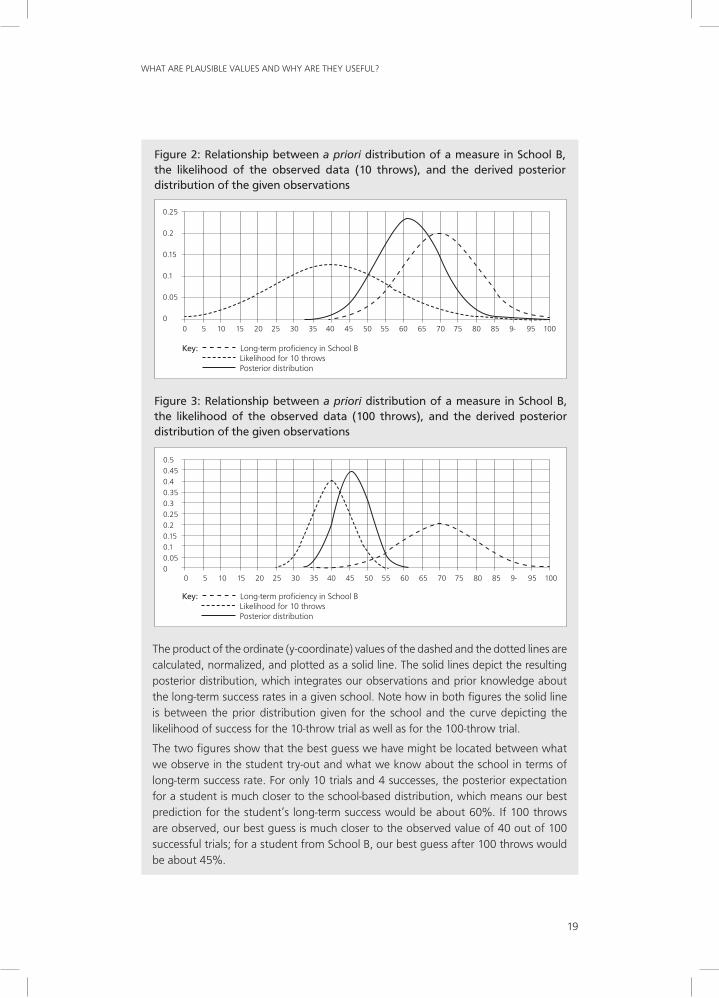
likelihoods, Prior Information, and Posteriors

Figures 2 and 3 illustrate how we obtained the numbers in Table 6. The two figures show an abscissa (x-coordinate) axis that represents the long-term success rate expressed as a percentage. The ordinate (y-coordinate) axis represents the function value of the continuous probability densities in the figures.

The figures include a dashed line that represents the probability density based on the assumption that the long-term success rate is normally distributed, with an expectation of 70% and a standard deviation of 10% in School B. The two dotted plots in the figures represent different amounts of information gathered (the likelihood) from observing 10 throws and four successes (represented in Figure 2), or from observing 100 throws and 40 successes (represented in Figure 3).

19


The product of the ordinate (y-coordinate) values of the dashed and the dotted lines are calculated, normalized, and plotted as a solid line. The solid lines depict the resulting posterior distribution, which integrates our observations and prior knowledge about the long-term success rates in a given school. Note how in both figures the solid line is between the prior distribution given for the school and the curve depicting the likelihood of success for the 10-throw trial as well as for the 100-throw trial.

The two figures show that the best guess we have might be located between what we observe in the student try-out and what we know about the school in terms of long-term success rate. For only 10 trials and 4 successes, the posterior expectation for a student is much closer to the school-based distribution, which means our best prediction for the student’s long-term success would be about 60%. If 100 throws are observed, our best guess is much closer to the observed value of 40 out of 100 successful trials; for a student from School B, our best guess after 100 throws would be about 45%.

Figure 2: Relationship between a priori distribution of a measure in School B, the likelihood of the observed data (10 throws), and the derived posterior distribution of the given observations

Key: Long-term proficiency in School B Likelihood for 10 throws Posterior distribution

0.25

0.2

0.15

0.1

0.05

00 5 10 15 20 25 30 35 40 45 50 55 60 65 70 75 80 85 9- 95 100

Key: Long-term proficiency in School B Likelihood for 10 throws Posterior distribution

0.50.450.40.350.30.250.20.150.10.050

0 5 10 15 20 25 30 35 40 45 50 55 60 65 70 75 80 85 9- 95 100

Figure 3: Relationship between a priori distribution of a measure in School B, the likelihood of the observed data (100 throws), and the derived posterior distribution of the given observations

20


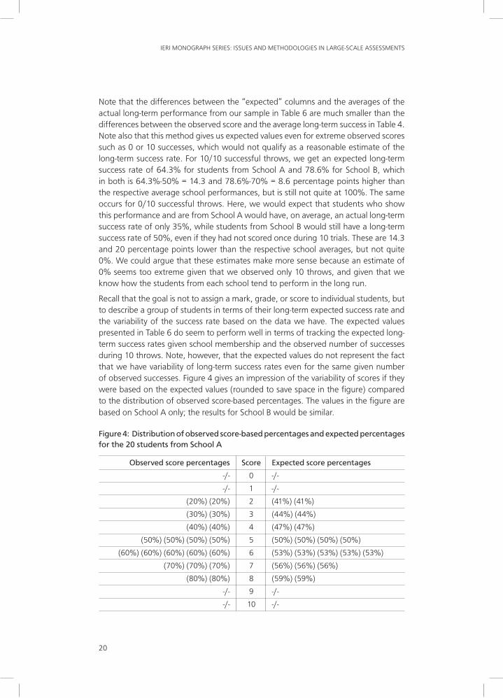
Note that the differences between the “expected” columns and the averages of the actual long-term performance from our sample in Table 6 are much smaller than the differences between the observed score and the average long-term success in Table 4. Note also that this method gives us expected values even for extreme observed scores such as 0 or 10 successes, which would not qualify as a reasonable estimate of the long-term success rate. For 10/10 successful throws, we get an expected long-term success rate of 64.3% for students from School A and 78.6% for School B, which in both is 64.3%-50% = 14.3 and 78.6%-70% = 8.6 percentage points higher than the respective average school performances, but is still not quite at 100%. The same occurs for 0/10 successful throws. Here, we would expect that students who show this performance and are from School A would have, on average, an actual long-term success rate of only 35%, while students from School B would still have a long-term success rate of 50%, even if they had not scored once during 10 trials. These are 14.3 and 20 percentage points lower than the respective school averages, but not quite 0%. We could argue that these estimates make more sense because an estimate of 0% seems too extreme given that we observed only 10 throws, and given that we know how the students from each school tend to perform in the long run.

Recall that the goal is not to assign a mark, grade, or score to individual students, but to describe a group of students in terms of their long-term expected success rate and the variability of the success rate based on the data we have. The expected values presented in Table 6 do seem to perform well in terms of tracking the expected long-term success rates given school membership and the observed number of successes during 10 throws. Note, however, that the expected values do not represent the fact that we have variability of long-term success rates even for the same given number of observed successes. Figure 4 gives an impression of the variability of scores if they were based on the expected values (rounded to save space in the figure) compared to the distribution of observed score-based percentages. The values in the figure are based on School A only; the results for School B would be similar.

Figure 4: Distribution of observed score-based percentages and expected percentages for the 20 students from School A

Observed score percentages Score Expected score percentages

-/- 0 -/-

-/- 1 -/-

(20%) (20%) 2 (41%) (41%)

(30%) (30%) 3 (44%) (44%)

(40%) (40%) 4 (47%) (47%)

(50%) (50%) (50%) (50%) 5 (50%) (50%) (50%) (50%)

(60%) (60%) (60%) (60%) (60%) 6 (53%) (53%) (53%) (53%) (53%)

(70%) (70%) (70%) 7 (56%) (56%) (56%)

(80%) (80%) 8 (59%) (59%)

-/- 9 -/-

-/- 10 -/-

21


In Figure 4, the score obtained in the 10-throw tryout for students from School A is associated with either the observed score-based percentage (on the left-hand side) or the expected values given in Table 5 on the right-hand side. When we calculate the variability of these measures based on the 20 values obtained from the left-hand side of Figure 4, we arrive at an estimate of 17.57 for the standard deviation of the observed score-based percentages, and an estimate of 5.01 for the standard deviation of the expected value-based measures on the right-hand side. The actual standard deviation of the sample, as given in Figure 1, is 9.5; the observation-only-based values over-estimate this value, while the expectation-based values under-estimate the actual variability of the long-term success rate in our sample.

uncertainty Where uncertainty Is DueThe expected values obtained from the free-throw score and prior knowledge based on school performance are useful in establishing that a result from a short tryout may not be the best predictor of long-term performance. This is especially the case when groups are concerned: we need to describe them in terms of statistical characteristics that are free from undesirable effects introduced by observing only a very small selection of the behavior of interest (as with the few trials in our example).

The “expected” values presented in Table 5 are surprisingly close to the actual average of the players given their observed performance. However, we found that the expected values did not reflect the reality of only a few trials; the true long-term success rate of students with the same number of successes on a short trial was still quite variable.

Unfortunately, the actual long-term success rates are not something we would have available. So how can we make up for the fact that the observed values do not serve our purpose, while the expected values do not vary “enough”? Note that Figure 4 reveals something peculiar about our use of the expectations we generated. We always replace the same observed score for a given school with the same expected percentage. In contrast, the actual long-term performances of students vary, even if they have the same observed number of successful throws. There is a way to reintroduce the knowledge that the long-term rate estimates are not certain even for the same observed score. This possibility also involves an application of Bayesian statistical methods.

We thus derived, in similar fashion to how we produced the expected values, a measure of variability around these expected values. Figures 3 and 4 showed that while we were able to derive an expected value for each set of numbers of throws, for successful throws, and for a given school, we still witnessed considerable variability around this expected value. A more appropriate representation of this remaining uncertainty can be gained by generating values that follow these posterior distributions. The values, randomly drawn from the posterior distribution show that, after 10 throws and knowing which school a student comes from, a considerable amount of uncertainty remains about this student’s probable long-term success rate. Even after 100 throws, we still see some uncertainty.

22


Within the context of large-scale survey assessments, random draws from posterior distributions are referred to as plausible values. We use this term here even though the plausible values in our example are based on a much reduced statistical model and are derived via our use of a number of simplifying assumptions. Table 7 shows the two sets of plausible values that were generated according to the procedure described above. The posterior distribution for each of the 20 students was generated as illustrated in Figure 3. The values in that figure drawn from the posterior distribution are depicted as solid lines.

Table 7: Examples of plausible values representing the expected values by observed score and the remaining variability of long-term expectations

First set of “plausible values” Second set of “plausible values”

0

1

38.2 43.9 2 38.8 36.2

45.1 36.1 3 47.1 39.1

58.5 43.1 4 45.5 48.5

42.6 47.5 39.8 47.0 5 39.6 55.3 49.0 45.7

43.5 65.4 66.8 50.1 54.8 6 37.5 34.6 31.4 42.9 56.7

55.4 67.5 7 65.4 61.0

57.9 48.2 8 58.9 59.5

9

10

Note: The two sets of plausible values are based on observed scores in School A.

As can be deduced from the information in Table 7, the mean for the first set of values is 50.1, and the standard deviation is 10.1. The mean for the second set is 47, and the standard deviation is 10.0. The values for the standard deviations are much closer to the value obtained for the actual long-term averages given in Figure 1 (9.5) when compared to the standard deviation based on expected values or observed score-based percentages.

The point that we want to make here is that the sets of plausible values give a more realistic representation of the expected values in subgroups as well as of the variances within actual results for these subgroups. Because the true values or, in our case, long-term averages are in most cases unknown, and because we do not have accurate estimates of individual performance on short tests, plausible values are a very useful tool for generating values that have more accurate statistical properties than do observed scores for subgroup comparisons. In our simple example, we had the true values available all along, and therefore did not need to use made-up plausible values. However, if we do not have the true values (and that is generally the case in real applications), plausible values can help us represent how the true distribution of proficiencies (in basketball or other areas) might look in those instances where we have substantial information about groups of students, but not enough observations on each individual student.

23


In practice, more than two sets of plausible values are generated; most national and international assessments use five, in accordance with recommendations put forward by Little and Rubin (1987). These five plausible values can be used to generate estimates of the statistics of interest, and then combined using the appropriate expressions for the variance of these statistics of interest (see Equation 1 below; also Little & Rubin, 1987). In closing the example presented in this section, we note again that the size of the samples we used is much smaller than what would be considered a minimal group size suitable for reporting in operational settings.

Working with Plausible Values As is evident from the example above, we can repeat the drawing of plausible values several times, each time obtaining a slightly different result for the individuals, yet each time obtaining unbiased estimates of the mean and the standard deviation of the distribution overall, and of the subgroups. So what should we consider to be our results? While plausible values are simply random draws from the posterior distributions, and any one set of plausible values will give us unbiased estimates of group distributions and differences between subgroups, these values are not suitable “scores” for the individuals in our sample. The average of these estimates across the subgroups will give us the best estimates of the group-level statistics of interest. In general, for each application, five sets of plausible values are drawn, although more can be drawn. Summarizing the results using the plausible values requires calculating the statistic of interest using each of the plausible values, and then finally averaging the results. (We refer, later in this article, to this method as PV-R—“R” for right, that is, correct.)

Computing the variance within groups properly requires us to use K sets of plausible values (we often find K=5 sets of plausible values in public-use databases), and the appropriate expressions for the imputation variance as articulated by Little and Rubin (1987):

(1)

This expression is one that is commonly found for variance decompositions into the average of variance estimates V̂ (MPVi) of the statistic MPVi for each group of plausible values i and variance of the K plausible values-based statistics MPVi between the K groups,

1 K–1 ∑i (MPVi – MPV)2.

We might be tempted to take a shortcut by averaging the plausible values for each individual student and then calculating the statistics of interest only once by using these averages of the plausible values. (We refer to this method later in the article as PV-W—“W” for wrong, not correct.) Although this method allows us to obtain the same mean as is evident with the PV-R method, the variance and percentile estimates will be biased because the distribution will have shrunk.

V̂IMP= 1+ 1K

1 K–1 ∑i (MPVi – MPV)2 +

1K ∑i V̂ (MPVi)

24


In the next section, we take the conceptual descriptions based on the first example and put the developed concepts to work in a more realistic setting. We use, in this example, larger, more realistic sample sizes. We also use a data structure as well as models and derived statistics that are closer to the actual analytical procedures used in large-scale survey assessments.

A moRe ComPlex exAmPle

How plausible values are generated in large-scale surveys is somewhat more complex than the procedure in the illustration presented above. The reason for this is that survey assessments use a much more complex test design than the 10-free-throw basketball test, which assumes all students are examined by repeating the same task multiple times. As we explained in the introduction, survey assessments include a large number of cognitive tasks or test items, which are administered to a sample of students, with each student taking only a subset of these items. Each of the several test booklets contains a fraction of the total set of test items. The items are systematically arranged into blocks and then combined into booklets, so that each item appears in exactly one block, and each block of items appears once in each of the several block-order positions within the booklets administered to students.

The large number of booklets containing different block combinations establishes an assessment design with many test forms. Because of the large number of blocks being used to cover a broad construct domain such as Grade 9 mathematics, it is often impossible to combine every block with all other blocks. This complex design of survey assessments makes traditional observed-score methods rather difficult or impossible to apply. Methods from modern test theory are applied to analyze the data and link the booklets, enabling reporting of results on one common scale. More specifically, methods based on the Rasch model (Rasch, 1980) or item response theory (IRT) (Lord & Novick, 1968) are applied and extended to allow the integration of covariates collected in background questionnaires alongside data from the test booklets.

Details about the assessment design used in international and national educational survey assessments can be found in, for example, Beaton, Mullis, Martin, Gonzalez, Kelly, and Smith (1996). Von Davier, Sinharay, Oranje, and Beaton (2007) consider current operational analyses methods for these assessments, and describe how these approaches integrate IRT and regression models for latent variables in order to facilitate reporting and the drawing of plausible values. Relatively complex models such as these used in large-scale surveys can be viewed as constrained but fine-grained versions of multiple-group IRT models. For our current purpose, however, these extensions of IRT models form the basis on which we can draw plausible values in practice.

25


using Plausible Values and Background DataHere, we use a simulated dataset to demonstrate the statistical difficulties encountered when aggregating individual “scores” for reporting group-level results. The advantage of using a simulated dataset is that we know the exact values (the “truth”) on which we based our simulation. Knowing the truth is useful when comparing different estimates that try to recapture these true values.

For our example, we generated mathematics proficiency-skill-levels for 4,000 cases crossing two “known” background characteristics: school type with levels A and B; and parental socioeconomic status (SES), also with two levels, H and L. This approach resulted in four (2x2) distinct groups, each with 1,000 cases. The average difference in mathematics skills between School Types A and B was 0.000 in our simulation, while the average difference based on parental SES was magnitude 1.414. The average for the high (H) SES group was +0.707, and -0.707 for the low (L) SES group. Let us ignore for now considerations as to whether these assumptions are particularly realistic or unrealistic, especially given that these variables may bear different effects in different populations. Table 8 presents the means and standard deviations used to generate the response data. We set the standard deviation within each of these groups to 0.707, which yielded a variance within each of the four groups of about 0.5 (or 0.7072), and an overall variance and standard deviation of 1.000.

Table 8: Means and standard deviations (in parenthesis) used to generate the simulated dataset

School

SES A B Average

L - 0.707 (0.707) - 0.707 (0.707) - 0.707 (0.707)

H +0.707 (0.707) +0.707 (0.707) +0.707 (0.707)

Total 0.000 (1.000) 0.000 (1.000) 0.000 (1.000)

For this example, we simulated the responses to a pool of 56 items for all the students in our dataset. The responses were simulated under three different conditions:

1. Items were randomly assigned to one of seven blocks, named A, B, C, D, E, F, and G. Every student responded to three of these blocks (24 items in total) in the assessment pool. The design organized the blocks according to this pattern: (ABD) (BCE) (CDF) (DEG) (EFA) (FGB) (GAC).

2. Using the same blocks composed for (1), every student responded to two of the blocks (16 items in total) in the assessment pool. The blocks were organized in seven pairs as follows: (AB) (BC) (CD) (DE) (EF) (FG) (GA).

3. Items were randomly assigned to one of 14 blocks, named A through N. Every student responded to two of these blocks (eight items in total) in the assessment pool. These blocks were organized in 14 pairs: (AB) (BC) (CD) (DE) (EF) (FG) (GH) (HI) (IJ) (JK) (KL) (LM) (MN) (NA).

26


We then calibrated the items using Parscale Version 4.1 (Muraki & Bock, 1997), and assigned scores to students via four different methods:

1. Expected-a-posteriori using Parscale (EAP);

2. Expected-a-posteriori using DESI (Gladkova, Moran, & Blew, 2006), taking into account group membership (EAP–MG);

3. Warm’s maximum likelihood estimates using Parscale (WML); and

4. Plausible values using DESI (PV-W and PV-R). Note that in our example each student was assigned five plausible values. For illustrative purposes, we can compute and present group statistics using plausible values in two ways. The first, PV-W (W for “wrong”), is calculated by taking the average of the plausible values for each student and using this value for our calculations. The second, PV-R (R for “right”), is calculated using each of the plausible values to compute the statistic of interest and then averaging the results over the five calculations.

We will begin by taking a look at the simulated data in order to determine the presence of any of the peculiarities we described earlier in this article. We will use our most extreme simulations, the ones in which each student was administered only 16 or 8 items, and where the number of correct scores could accordingly range from 0 through 16 in one case, and between 0 and 8 in the other. Keep in mind that in our simulation there is no school effect, so the overall school means are the same. However, remember also that we built in an SES effect such that those in the group SES Type H scored higher than those in SES Type L.

Table 9 shows, for each school type, the number of students in our simulated dataset obtaining each “number correct” score on the 16-item test. We also show these students’ average true score by school type and the difference between the average true score for the students obtaining the same number correct.

Notice from the table how the students for each score point come from both school types, in quite similar numbers for most observed scores. Those who score 0 are 41 students from School A and 38 students from School B. As we go down the table, we observe only small differences for most score points. We can also see that the average difference in the average generating ability is close to 0 across the range of number correct scores.

Table 10 shows similar results for the simulated students from School Types A and B who took only 8 items. Again, we observe that the students are fairly evenly distributed across the two school types for each number correct score, and that the average true score differences between schools is again close to 0. We can expect this outcome, because, as we mentioned earlier, we did not introduce differences between school types in our simulation. We also found that where there were no differences between school types, our estimates were fairly consistent when we compared the results of the 16-item test and the 8-item test. If we wanted to obtain the mean by school type, we would simply, in both cases, multiply the average generating ability for each number correct group by the number of cases, and divide by the total number of cases.

27


Table 9: Average generating ability and number of cases, by school type on the simulated 16-item test

Average generating Number of cases ability (or “truth”)

Number correct School Type A School Type B School Type A School Type B Average difference

0 -1.668 -1.825 41 38 0.157

1 -1.562 -1.564 91 83 0.002

2 -1.274 -1.257 119 122 - 0.017

3 - 0.979 -1.008 140 137 0.029

4 - 0.852 - 0.823 127 125 - 0.028

5 - 0.652 - 0.611 123 139 - 0.041

6 - 0.457 - 0.455 125 139 - 0.002

7 - 0.272 - 0.215 156 125 - 0.057

8 - 0.054 - 0.058 136 141 0.004

9 0.160 0.111 125 128 0.049

10 0.349 0.391 133 111 - 0.042

11 0.514 0.462 134 130 0.052

12 0.696 0.703 133 129 - 0.007

13 0.929 0.924 127 136 0.006

14 1.139 1.254 131 128 - 0.115

15 1.491 1.465 108 133 0.026

16 1.660 1.802 51 56 - 0.142

Table 10: Average generating ability and number of cases, by school type on the simulated 8-item test


Number correct School Type A School Type B School Type A School Type B Average difference

0 -1.458 -1.409 138 139 - 0.048

1 -1.065 -1.141 239 205 0.077

2 - 0.735 - 0.787 243 248 0.052

3 - 0.414 - 0.391 240 250 - 0.023

4 - 0.046 - 0.036 255 241 - 0.010

5 0.335 0.328 245 257 0.006

6 0.624 0.629 271 230 - 0.005

7 1.068 1.075 223 264 - 0.007

8 1.386 1.398 146 166 - 0.013

28


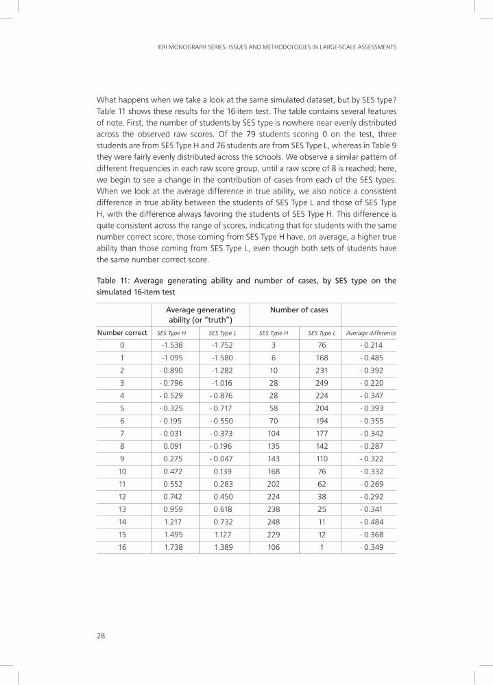
What happens when we take a look at the same simulated dataset, but by SES type? Table 11 shows these results for the 16-item test. The table contains several features of note. First, the number of students by SES type is nowhere near evenly distributed across the observed raw scores. Of the 79 students scoring 0 on the test, three students are from SES Type H and 76 students are from SES Type L, whereas in Table 9 they were fairly evenly distributed across the schools. We observe a similar pattern of different frequencies in each raw score group, until a raw score of 8 is reached; here, we begin to see a change in the contribution of cases from each of the SES types. When we look at the average difference in true ability, we also notice a consistent difference in true ability between the students of SES Type L and those of SES Type H, with the difference always favoring the students of SES Type H. This difference is quite consistent across the range of scores, indicating that for students with the same number correct score, those coming from SES Type H have, on average, a higher true ability than those coming from SES Type L, even though both sets of students have the same number correct score.

Table 11: Average generating ability and number of cases, by SES type on the simulated 16-item test


Number correct SES Type H SES Type L SES Type H SES Type L Average difference

0 -1.538 -1.752 3 76 - 0.214

1 -1.095 -1.580 6 168 - 0.485

2 - 0.890 -1.282 10 231 - 0.392

3 - 0.796 -1.016 28 249 - 0.220

4 - 0.529 - 0.876 28 224 - 0.347

5 - 0.325 - 0.717 58 204 - 0.393

6 - 0.195 - 0.550 70 194 - 0.355

7 - 0.031 - 0.373 104 177 - 0.342

8 0.091 - 0.196 135 142 - 0.287

9 0.275 - 0.047 143 110 - 0.322

10 0.472 0.139 168 76 - 0.332

11 0.552 0.283 202 62 - 0.269

12 0.742 0.450 224 38 - 0.292

13 0.959 0.618 238 25 - 0.341

14 1.217 0.732 248 11 - 0.484

15 1.495 1.127 229 12 - 0.368

16 1.738 1.389 106 1 - 0.349

29


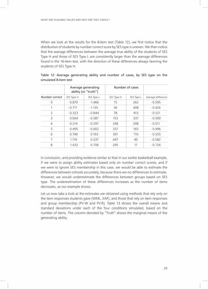
When we look at the results for the 8-item test (Table 12), we first notice that the distribution of students by number correct score by SES type is uneven. We then notice that the average differences between the average true ability of the students of SES Type H and those of SES Type L are consistently larger than the average differences found in the 16-item test, with the direction of these differences always favoring the students of SES Type H.

Table 12: Average generating ability and number of cases, by SES type on the simulated 8-item test


Number correct SES Type H SES Type L SES Type H SES Type L Average difference

0 - 0.870 -1.466 15 262 - 0.595

1 - 0.711 -1.135 36 408 - 0.424

2 - 0.323 - 0.844 78 413 - 0.521

3 0.004 - 0.587 153 337 - 0.590

4 0.214 - 0.297 248 248 - 0.511

5 0.495 - 0.002 337 165 - 0.496

6 0.749 0.193 391 110 - 0.555

7 1.119 0.537 447 40 - 0.582

8 1.432 0.706 295 17 - 0.726

In conclusion, and providing evidence similar to that in our earlier basketball example, if we were to assign ability estimates based only on number correct scores, and if we were to ignore SES membership in this case, we would be able to estimate the differences between schools accurately, because there are no differences to estimate. However, we would underestimate the differences between groups based on SES type. The underestimation of these differences increases as the number of items decreases, as our example shows.

Let us now take a look at the estimates we obtained using methods that rely only on the item responses students gave (WML, EAP), and those that rely on item responses and group membership (PV-W and PV-R). Table 13 shows the overall means and standard deviations under each of the four conditions simulated, based on the number of items. The column denoted by “Truth” shows the marginal means of the generating ability.

30


Table 13: Overall means and standard deviations of the simulated scores

Mean Standard deviation

Number Truth EAP EAP- WML PV-W PV-R Truth EAP EAP- WML PV-W PV-Rof items (MG) (MG)

24 - 0.01 0.01 0.01 0.01 0.01 0.01 0.99 0.96 0.95 1.05 0.95 0.99

16 - 0.01 0.01 0.02 0.02 0.02 0.02 0.99 0.94 0.93 1.06 0.94 0.99

8 - 0.01 0.00 0.01 0.00 0.00 0.00 0.99 0.87 0.87 1.02 0.88 0.97

Notice that while the means in Table 13 have been predicted fairly accurately regardless of the number of items and the scoring method used, this is not the case for the estimated standard deviations. Except for the value in the column headed PV-R, the standard deviation (and, as a consequence, the overall estimate of the variance) is generally under-predicted, with a noticeable deterioration as the number of items decreases.

Notice also that although the mean estimates using PV-W and PV-R are identical, this is not the case for the estimates of the standard deviations under these two conditions. PV-R (the averaged results from each of the five plausible values) provides an estimate that is indeed almost identical to the standard deviation of the generating ability. However, when we estimate the standard deviation using the averaged plausible values (PV-W), we consistently underestimate the true standard deviation. The WML estimates start by overestimating the standard deviation, but as the number of items decreases, the standard deviation is underestimated, as it is with the EAP method and the EAP-MG method. When we use plausible values the “right” way (PV-R), we do obtain a relatively good and stable estimate of the standard deviation, even as the number of items reaches down to 8.

Tables 14 and 15 show the marginal means and standard deviations for each of the groups as obtained from the simulated data. The values shown are the sample means for the marginal distributions by school type and by SES.

Table 14: Marginal averages and standard deviations in subgroups defined by school type, and the corresponding EAP, WML, and PV aggregates


Number School Truth EAP EAP- WML PV-W PV-R Truth EAP EAP- WML PV-W PV-Rof items type (MG) (MG)

24 A - 0.03 0.01 0.01 0.01 0.01 0.01 0.98 0.95 0.94 1.03 0.94 0.98

16 A - 0.03 0.00 0.00 0.00 0.00 0.00 0.98 0.93 0.92 1.05 0.93 0.98

8 A - 0.03 - 0.01 - 0.02 - 0.02 - 0.02 - 0.02 0.98 0.86 0.86 1.01 0.87 0.95

24 B 0.01 0.02 0.02 0.02 0.02 0.02 1.01 0.96 0.95 1.06 0.96 1.00

16 B 0.01 0.03 0.03 0.04 0.03 0.03 1.01 0.94 0.94 1.07 0.95 1.01

8 B 0.01 0.02 0.03 0.02 0.03 0.03 1.01 0.87 0.88 1.03 0.90 0.98

31


In Table 14 we observe a similar pattern to that observed in Table 13. The means are estimated fairly well by all methods used, with the PV-W and the PV-R coinciding exactly. But when we look at the standard deviations, we again see a deterioration in these estimates as the number of items decreases. In particular, notice how, when we use the plausible values in the correct way (PV-R), our estimates of the subgroup means and the standard deviations of the groups are estimated consistently.

When using any of the other methods, we are able to estimate only the mean correctly, but not the standard deviation. This is also why plausible values are crucial for estimating proportion-above-point scores, such as proportion of students at or above proficient, which is what so many large-scale assessment program inferences are based on. However, keep in mind that when conducting our simulation, we specified that there should be no differences between the school types, and this is what we observed. This is not the case when we look at the results for the SES types shown in Table 15.

Table 15: Marginal averages and standard deviations in subgroups defined by SES, and the corresponding EAP, WML, and PV aggregates


Number SES Truth EAP EAP- WML PV-W PV-R Truth EAP EAP- WML PV-W PV-Rof items type (MG) (MG)

24 H 0.69 0.66 0.71 0.71 0.71 0.71 0.72 0.71 0.64 0.79 0.66 0.71

16 H 0.69 0.63 0.71 0.70 0.71 0.71 0.72 0.72 0.64 0.84 0.65 0.73

8 H 0.69 0.56 0.69 0.64 0.68 0.68 0.72 0.66 0.53 0.80 0.56 0.69

24 L - 0.71 - 0.64 - 0.69 - 0.68 - 0.68 - 0.68 0.70 0.70 0.63 0.77 0.65 0.70

16 L -0.71 - 0.60 - 0.68 - 0.66 - 0.67 - 0.67 0.70 0.69 0.61 0.78 0.63 0.70

8 L - 0.71 - 0.55 - 0.68 - 0.63 - 0.67 - 0.67 0.70 0.67 0.54 0.80 0.57 0.69

In this table, we observe a somewhat different pattern to the one observed in the previous tables. Keep in mind that Table 15 shows us the marginal means and standard deviations for the groups as defined by the grouping variable SES, and that we simulated differences between these two groups. Unlike the previous tables, the EAP and WML results in Table 15 show a bias of the subgroup means toward the overall mean (0.00) as the number of items decreases. However, the results for the EAP-MG, PV-W, and PV-R provide us with means that are fairly close to the means of the generating distribution. When we look at the standard deviations by subgroups, we again see that the only method by which we obtain standard deviations consistent with the generating distribution, and regardless of the number of items administered, is when we compute these statistics using plausible values in the prescribed way (PV-R). In conclusion, it seems that plausible values, when analyzed properly, give us unbiased estimates for the overall mean and the standard deviations of the subgroups of interest.

32


Let us go back again to our example to see whether using the plausible values as estimates of the average group performance allows us to reproduce the results presented at the beginning of this section. For this purpose, we compute the average raw score for each of the subgroups of interest and compare these with the results observed from the generating or true scores.

As we can see in Table 16, extremely small to no differences by school type are evident in our simulated data (column “Truth”), and there are no differences relative to the estimates we calculated in our analysis. However, when we look at the same data analyzed by SES type (Table 17), we notice a different pattern. For example, while the true scores show differences between SES Type L and SES Type H for each number correct score, the difference always favors SES Type H. Neither WML nor the EAP estimates is able to capture this difference. While the differences slightly favor the SES Type H group, these are clearly underestimates when compared with what we would expect to find based on the true scores used to generate the data. When we look at the EAP-(MG) and the PV-W and PV-R results, we notice that the difference between the groups, while not reflected exactly, does show up fairly well in our analysis. Curiously, but not unexpectedly, the results using PV-W and PV-R are exactly the same because the computation of these means is algebraically equivalent. However, remember that in our previous tables the results we obtained using PV-W underestimated the variances for the subgroups.

Table 16: Difference in average scores between School Type A and School Type B, by number correct on the 8-item test

Number Truth WML EAP EAP-(MG) PV-W PV-R correct

0 - 0.048 0.001 - 0.005 - 0.005 0.028 0.028

1 0.077 0.006 0.003 0.008 0.036 0.036

2 0.052 - 0.006 - 0.005 - 0.022 0.006 0.006

3 - 0.023 0.007 0.009 - 0.010 - 0.033 - 0.033

4 - 0.010 0.018 0.015 0.013 - 0.002 - 0.002

5 0.006 0.010 0.010 0.020 0.011 0.011

6 - 0.005 0.010 0.010 - 0.018 - 0.007 - 0.007

7 - 0.007 - 0.024 - 0.018 - 0.055 - 0.087 - 0.087

8 - 0.013 0.010 0.006 - 0.030 - 0.073 - 0.073

33


Table 17: Difference in average scores between SES Types L and H, by number correct on the 8-item test

Number Truth WML EAP EAP-(MG) PV-W PV-R correct

0 0.595 -0.011 0.025 0.678 0.651 0.651

1 0.424 0.084 0.067 0.609 0.611 0.611

2 0.521 0.080 0.072 0.554 0.524 0.524

3 0.590 0.094 0.086 0.532 0.542 0.542

4 0.511 0.082 0.077 0.513 0.490 0.490

5 0.496 0.072 0.065 0.511 0.503 0.503

6 0.555 0.068 0.060 0.541 0.529 0.529

7 0.582 0.097 0.076 0.607 0.517 0.517

8 0.726 0.109 0.054 0.684 0.736 0.736

One last inspection of the data will help us see the advantages of using the plausible values in the correct way, even if the EAP-(MG) and the PV-W give point estimates quite similar to those given by PV-R. Table 18 shows the percentiles of the distribution of scores using the 8-item test, calculated with each one of the estimates obtained from the simulated data. The sum of the squared difference gives us a measure of how different our estimated percentiles are over the distribution. Notice that when we look at the distribution of scores, the squared differences between percentiles are relatively small and the percentile estimates using PV-R come closest to the percentiles from the true distribution. Notice also that the estimates obtained using PV-R more closely estimate the extreme percentiles (10th and 90th).

Table 18: Percentiles of the distribution and the sum of the squared differences between the estimated scores and the truth

Percentile Truth WML EAP EAP-(MG) PV-W PV-R

10 -1.295 -1.256 -1.149 -1.161 -1.188 -1.276

20 - 0.912 - 0.870 - 0.829 - 0.871 - 0.855 - 0.872

30 - 0.611 - 0.554 - 0.542 - 0.597 - 0.580 - 0.565

40 - 0.307 - 0.266 - 0.260 - 0.294 - 0.285 - 0.280

50 - 0.023 0.015 0.014 0.026 0.018 0.008

60 0.267 0.266 0.267 0.305 0.298 0.289

70 0.561 0.538 0.535 0.591 0.576 0.569

80 0.887 0.857 0.837 0.889 0.858 0.884

90 1.305 1.350 1.217 1.191 1.203 1.271

Sum of the squared differences between truth and estimated percentiles

0.013 0.047 0.037 0.030 0.007

34


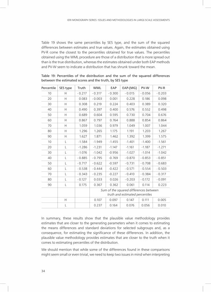
Table 19 shows the same percentiles by SES type, and the sum of the squared differences between estimates and true values. Again, the estimates obtained using PV-R come the closest to the percentiles obtained for true values. The percentiles obtained using the WML procedure are those of a distribution that is more spread out than is the true distribution, whereas the estimates obtained under both EAP methods and PV-W seem to indicate a distribution that has shrunk toward the mean.

Table 19: Percentiles of the distribution and the sum of the squared differences between the estimated scores and the truth, by SES type

Percentile SES type Truth WML EAP EAP-(MG) PV-W PV-R

10 H - 0.217 - 0.317 - 0.300 - 0.015 - 0.056 - 0.203

20 H 0.083 - 0.003 0.001 0.228 0.186 0.098

30 H 0.308 0.219 0.224 0.403 0.389 0.320

40 H 0.490 0.397 0.400 0.576 0.552 0.498

50 H 0.689 0.604 0.595 0.730 0.704 0.676

60 H 0.867 0.797 0.764 0.888 0.854 0.864

70 H 1.059 1.036 0.979 1.049 1.007 1.044

80 H 1.296 1.265 1.175 1.191 1.203 1.267

90 H 1.627 1.871 1.462 1.392 1.399 1.575

10 L -1.584 -1.949 -1.455 -1.401 -1.400 -1.561

20 L -1.286 -1.231 -1.147 -1.161 -1.187 -1.271

30 L -1.076 -1.042 -0.956 -1.027 -1.014 -1.042

40 L - 0.885 - 0.795 -0.769 - 0.870 - 0.853 - 0.851

50 L - 0.717 - 0.622 -0.597 - 0.731 - 0.708 - 0.683

60 L - 0.538 - 0.444 -0.422 - 0.571 - 0.554 - 0.503

70 L - 0.343 - 0.235 -0.227 - 0.410 - 0.384 - 0.317

80 L - 0.127 0.033 0.026 - 0.203 - 0.172 - 0.091

90 L 0.175 0.367 0.362 0.061 0.114 0.223

Sum of the squared differences between truth and estimated percentiles

H 0.107 0.097 0.147 0.111 0.005

L 0.237 0.164 0.076 0.056 0.010

In summary, these results show that the plausible value methodology provides estimates that are closer to the generating parameters when it comes to estimating the means differences and standard deviations for selected subgroups and, as a consequence, for estimating the significance of these differences. In addition, the plausible value methodology provides estimates that are closer to the truth when it comes to estimating percentiles of the distribution.

We should mention that while some of the differences found in these comparisons might seem small or even trivial, we need to keep two issues in mind when interpreting

35


them. First, because the data used in these analyses are simulated and are based on a relatively simple model of group differences, the results are substantially more stable than those that would be found in real-life data. We can expect to find a greater and more noticeable effect when using real data with much larger amounts of background data, because these are collected in large-scale survey assessments. Second, and perhaps of more importance, large-scale assessment data are used to make educational policy decisions that affect many in the population. So, for example, when calculating the percentage of students reaching a benchmark in the population, a 2% difference can translate into many students classified as proficient or not proficient. Using appropriate statistical techniques can minimize the amount of misclassification.

CoNCluSIoN

In this article, we compared group-level estimates based on commonly used estimators of individual student scores with group-level estimates based on five separate calculations using plausible values. We found that both individual score-based methods (EAP and WML) bear undesirable effects that adversely affect their utility as a basis for accurate group-level statistics. First, we observed a noticeable bias toward more extreme values when generating student scores based on Warm’s maximum likelihood estimates (WML) using small numbers of items. Second, we showed that the expected a-posteriori (EAP) score of a student, given his or her set of responses and a (prior) distribution based on a sample of students from the same population, is biased toward the mean of this reference distribution.

Why do we see these undesirable effects in group-level variance estimates? As we stated above, maximum likelihood estimates tend to be “too extreme” when only a few item responses are involved. Our results have shown that the values in column “WML” of the relevant tables are comparably too large, indicating that the WMLs vary too much (are more extreme than the truth). With EAP-based standard deviations, these estimates are much smaller than the truth. From the point of view of individuals, EAPs “pull” toward the group mean in such a way that their expected value is the correct mean over individuals. From the point of view of individuals, PVs add noise. But from the point of view of groups, they add exactly the right amount of variability to make the distribution of the PVs in the group match the distribution of the true values in the group.

The use of plausible values for group-level reporting has been advocated since the National Assessment of Educational Progress (NAEP) started utilizing this imputation technique. However, we stress here that plausible values are not suitable as individual scores, and they were never intended as such. They are a tool that enables official reporting and allows secondary analysts to operate on the same data.

One common misconception among those using plausible values is that the mean of plausible values can be used instead of the average over five calculations with the given set of plausible values. However, as evident from the examples in this article, the variance is severely underestimated for group-level calculations when this method

36


(PV-W(wrong)) or EAP scores are used. The EAP is the value that we can expect when we have at hand item responses and background data, and it is about the value we can expect to get when averaging the five plausible values of a given student. Thus, using the average of five plausible values should result in the same severe underestimation of group-level variability as using the EAP, a situation that we should obviously avoid.

As we stated at the beginning of this article, analysts do not need to rely on computational shortcuts by averaging plausible values before conducting calculations: analytical shortcuts such as averaging plausible values produce biased estimates and should therefore be discouraged. The procedures developed in the relevant literature should be followed or software employed that is already set up to use plausible values with the appropriate procedures.3 These tools, which have become increasingly easy to use, provide analysts with appropriate methodologies and procedures for analyzing the information contained in large-scale survey databases.

ReferencesBeaton, A. E., Mullis, I. V. S., Martin, M. O., Gonzalez, E. J., Kelly, D. L., & Smith, T. A. (1996). Mathematics achievement in the middle school years: IEA’s Third International Mathematics and Science Study. Chestnut Hill, MA: Boston College.

Gladkova, L., Moran, R., & Blew, T. (2006). Direct Estimation Software Interactive (DESI) manual. Princeton, NJ: Educational Testing Service.

Little, R. J. A., & Rubin, D. B. (1987). Statistical analysis with missing data. New York: J. Wiley & Sons.

Lord, F. M., & Novick, M. R. (1968). Statistical theories of mental test scores. Reading, MA: Addison-Wesley.

Mislevy, R. J. (1991). Randomization-based inference about latent variables from complex samples. Psychometrika, 56(2), 177–196.

Mislevy, R. J. (1993). Should “multiple imputations” be treated as “multiple indicators”? Psychometrika, 58(1), 79–85.

Muraki, E., & Bock, R. D. (1997). PARSCALE: IRT item analysis and test scoring for rating-scale data (computer software). Chicago: Scientific Software.

Rasch, G. (1980). Probabilistic models for some intelligence and attainment tests. Chicago: The University of Chicago Press.

Schafer, J. L. (1997). Analysis of incomplete multivariate data. London: Chapman & Hall.

von Davier, M., Sinharay, S., Oranje, A., & Beaton, A. (2007). The statistical procedures used in National Assessment of Educational Progress: Recent developments and future directions. In C. R. Rao & S. Sinharay (Eds.), Handbook of statistics: Vol. 26. Psychometrics (pp. 1039–1055). Amsterdam: Elsevier.

3 Several software programs allow the use of multiple imputations, or are already set up to allow various analyses of information contained in the databases of large-scale survey assessments. Examples are the NAEP Data Explorer available at http://nces.ed.gov/nationsreportcard/nde/ through the National Center for Education Statistics (NCES); the latest version of the HLM software (http://www.ssicentral.com/hlm/index.html); AIR’s AM software (http://am.air.org/); and the SPSS-based International Association for the Evaluation of Educational Achievement International Database Analyzer (IEA IDB Analyzer) (http://www.iea.nl/iea_studies_datasets.html).

What are plausible values and why are they useful? · PDF fileWhat are plausible values and...

Documents

Transcript of What are plausible values and why are they useful? · PDF fileWhat are plausible values and...