Wharton-SMU Research Center

International Capital Markets and Foreign Exchange Risk

Yihong Xia and Michael J. Brennan

This project is funded by the Wharton-SMU Research Center of Singapore Management University

International Capital Markets and ForeignExchange Risk∗

Michael J. Brennan and Yihong Xia†

July 18, 2003

∗We thank Lim Kian Guan for many helpful conversations. Brennan thanks Lancaster Univer-sity for their hospitality. Xia thanks the Singapore Management University for their hospitalityand gratefully acknowledges the financial support from the Wharton-SMU Research Center of theSingapore Management University.

†Michael Brennan is Emeritus Professor at the Anderson School, UCLA, 110 Westwood Plaza, LosAngeles, CA 90095-1481. Yihong Xia is an assistant professor at the Wharton School of Universityof Pennsylvania. Corresponding address: Finance Department, The Wharton School, Universityof Pennsylvania; 2300 Steinberg Hall-Dietrich Hall; Philadelphia, PA 19104-6367. Phone: (215)898-3004. Fax: (215) 898-6200. E-mail: yxia@wharton.upenn.edu.

Abstract

A relation between the volatilities of the pricing kernels for different cur-rencies is derived under the assumption of integrated capital markets, and thevolatility of the pricing kernel is related to the foreign exchange risk premium.The time series of the pricing kernel volatilities are estimated from panel dataon bond yields for five major currencies using a parsimonious term structuremodel that allows for time varying risk premia. The resulting estimates areused to estimate the relation between the volatilities of the pricing kernels indifferent currencies and the volatility of the exchange rate. It is also shown thattime variation in the foreign exchange risk premium is related to time variationin the volatility of the pricing kernel for certain currencies.

1 Introduction

The issue of capital market integration is of central importance in the theory

of international finance since it has important implications for asset pricing as well

as for optimal portfolio choice. Tests of asset pricing models typically rely on an

assumption about international capital market integration which becomes part of

the maintained hypothesis. For example, tests of national versions of the Capital

Asset Pricing Model (CAPM) rely on the implicit assumption of segmented national

capital markets, while tests of a world CAPM (see, for example, Harvey (1991)), a

world CAPM with exchange risk (see Dumas and Solnik (1995)), or world multi-factor

models (Ferson and Harvey (1994)) are all based on the assumption of integrated

world markets. An intermediate assumption is that markets are partially integrated.

For example, Bekaert and Harvey (1995) adopt a parameterized model of partial

integration within a regime-switching model in which expected returns on a country

market index are determined by both their covariance with a world market portfolio

and the own-variance of the country market returns. In a perfectly integrated market,

only the world market covariance counts, while in a perfectly segmented market only

the own-variance is relevant. Their integration measure is a time-varying weight that

is applied to the covariance and the own-variance. This approach to assessing market

integration relies on an underlying single-period beta pricing model which is assumed

to apply to equity market returns. In a more recent paper, Bekaert, Harvey and

Lumsdaine (2001) specify a reduced-form model for several financial time-series and

search for a common, endogenous break in the process that would indicate a change

from segmentation to integration.

These studies of international market integration are based either on equity mar-

ket returns or on the behavior of macroeconomic variables. In this paper on the

other hand we assess the integration of capital markets using data on bond prices

for different countries. Since government bonds in developed economies are virtually

1

default free, are traded in markets that are highly liquid, and are less likely than

stock markets to suffer from problems of informational asymmetry between foreign

and domestic investors,1 these markets offer a natural setting for assessing the degree

of capital market integration.

The paper relies on recent evidence of time variation in risk premia in US bond

and stock markets and uses the fact that in integrated capital markets the time

variation in risk premia in different markets will be related; more precisely, the time

variation in risk premia of bonds denominated in different currencies will be related.

The nature of the relation is made precise by first deriving the relation between the

volatilities of the pricing kernels for returns denominated in different currencies for

general arbitrage free markets. The volatility of the pricing kernel is the maximum

“Sharpe ratio” for returns denominated in that currency. Then the volatilities of

the pricing kernels are estimated by making use of a parsimonious valuation model

developed by Brennan, Wang and Xia (2003) that allows for time variation in risk

premia. The model assumes that the real interest rate and the maximum “Sharpe

ratio” for each currency follow correlated Ornstein-Uhlenbeck processes.2 While these

two “state” variables are not directly observable, the valuation model allows us to

estimate them, along with the expected rate of inflation, from panel data on default-

free bond yields and inflation. We carry out the estimation for the United States, the

United Kingdom, Japan, Germany, and Canada.

If the markets for returns denominated in two different currencies are integrated,

then a simple linear relation obtains between the estimated Sharpe ratios for the

currencies, and the volatility of the rate of exchange between them. We test this

1Brennan and Cao (1997) and Brennan et al. (2003) show that international trading in equities isconsistent with informational asymmetries between local and foreign investors. Portes et al. (2001)show that the pattern of international bond trading is less influenced by informational considerationsthan is the pattern of stock trading.

2Note that the real interest rate for two different currencies can differ because the price indicesthat are used for the currencies differ and because the inflation risk of the currencies differ.

2

hypothesis across country pairs using our estimates of the Sharpe ratios.

Finally, we use the pricing kernel framework to cast further light on the “forward

premium puzzle.” An extensive empirical literature documents the failure of uncov-

ered interest parity (UIP) and shows that there is often a “perverse” relation between

the interest rate differential and the realized exchange rate change, which constitutes

the puzzle.3 Fama (1984) argues that the failure of UIP is associated with evidence of

a time-varying foreign exchange risk premium. Adler and Dumas (1993) develop an

international version of the Capital Asset Pricing Model (CAPM) in which the risk

premium on an asset depends on market risk, as measured by the covariance between

returns on the asset return and the market portfolio, and currency risk, as measured

by the sum of covariances between the asset return and the currency returns.4 While

earlier studies such as Giovannini and Jorion (1989) and Jorion (1989) found no ev-

idence that exchange rate risk was priced in equity markets, more recent papers,

including Korajczyk and Viallet (1990), Dumas and Solnik (1995) and De Santis and

Gerard (1998), have found that exchange rate risk is a statistically significant priced

factor, and that the International CAPM performs better than the standard CAPM

which ignores currency risk. Moreover, Dumas and Solnik (1995) and De Santis and

Gerard (1998) report evidence of time-variation in exchange rate risk.

If the pricing kernel is directly specified, then it is straightforward to determine

whether foreign exchange risk is priced. The valuation model that we develop does

not specify the pricing kernel itself, but only the instantaneous drift and volatility

3Hollifield and Uppal (1997) find that segmented commodity markets can lead to a deviation ofUIP but fail to explain the negative relation between the expected change in exchange rates andinterest rate differentials. Bansal (1997) finds that violation of UIP depends on the sign of theinterest rate differential. Meredith and Chinn (1998) finds that UIP holds better at the five to tenyear horizon.

4Other attempted explanations of the “forward premium puzzle” include 1) changing secondmoments as in Hansen and Hodrick (1983), Domowitz and Hakkio (1985), and Cumby (1988); 2)non-additive utility functions as in Backus, Gregory and Telmer (1993), Bansal (1996) and Bekaert(1996); and 3) commodity market segmentation due to transportation costs as in Hollifield andUppal (1997).

3

of the pricing kernel, which correspond respectively to the real interest rate and the

maximum Sharpe ratio for the currency. However, if the correlation of the exchange

rate with the pricing kernel is constant, as we shall assume, then time series variation

in the volatility of the pricing kernel will be mirrored in variation in the foreign

exchange risk premium. Therefore we examine the relation between the estimated

volatilities of the pricing kernels for the different currencies and the foreign exchange

risk premium.

Our continuous-time model of the joint dynamics of interest rates in two countries

and of the exchange rate between them is similar in spirit to the models developed in

Nielsen and Saa-Requejo (1993), Saa-Requejo (1993), Ahn (1995), Bansal (1997),

Backus, Foresi and Telmer (2001), Brandt and Santa-Clara (2002), and Brandt,

Cochrane and Santa-Clara (2003). In all the papers including this one, the pric-

ing kernel for the domestic and foreign countries is either derived from a general

equilibrium setting or is specified exogenously, and then the relation between the for-

eign exchange rate dynamics and the two pricing kernels is derived from no-arbitrage

arguments. Data from foreign exchange rates and short term interest rates are gen-

erally used to examine the model implications. These papers differ from one another

mainly in how the pricing kernel and the term structure are specified in each country

and thus how the empirical implications are tested. All the papers listed above use

complete affine term structure models and only use short term interest rates to proxy

for instantaneous interest rates instead of estimating the term structure using zero-

coupon bond yields with different maturities, which is the norm in the single country

term structure literature.

In this paper, we use instead a parsimonious essentially affine model which has

more flexibility in modeling risk premia.5 Because the model contains unobservable

5The distinction between an affine model and an essentially affine model is that the compensationfor interest rate risk can vary independently of interest rate volatility in an essentially affine modelwhile this is not the case in a complete affine model. See Duffee (2002) for more details.

4

state variables that are directly related to foreign exchange rates, we estimate the

model parameters and state variables from bond yields, and finally test the model

implications for the exchange rates of five developed economies using the state vari-

ables estimated from the bond yield data.

To summarize our empirical results, the state variable and model parameter esti-

mates that are obtained from the bond yield data for the different currencies confirm

that real interest rate risk is priced in all five currencies. In contrast, there is no

evidence that the risk associated with innovations in expected inflation commands a

risk premium. However, innovations in the maximum Sharpe ratio, η, command a

positive risk premium for all currencies but the Japanese Yen, where the variation in

this variable is much lower than in the other countries and is statistically insignifi-

cant. Estimates of lagged cross-effects between currencies for real interest rates and

for the pricing kernel volatility are consistent with capital market integration, the

estimated correlation matrices for state variable innovations providing evidence of

common shocks across capital markets. The linkages between Canada and the US

and between Germany and the UK are particularly strong, while those between Japan

and all the other countries are particularly weak; while there is evidence that the bond

pricing model is particularly mis-specified for Japan, this suggests that geographic

proximity may be important.

We find that the volatility of the pricing kernels for different currencies are posi-

tively related as the theory predicts. Moreover, the relation appears to be stronger in

the period after 1994. We also find that time variation in the foreign exchange risk

premium is associated with variation in the volatility of the pricing kernels, especially

that of the pricing kernel associated with the U.S. dollar.

The rest of the paper is organized as follows. The second and third sections provide

the definition of real and nominal pricing kernels in domestic and foreign countries

and derive testable implications. Section 4 discusses the details of data construction

5

and reports descriptive statistics. Section 5 describes the estimation procedure and

the state variables. Section 6 reports empirical tests on market integration, the reward

to foreign exchange rate risk, and the forward premium puzzle. Section 7 summarizes

and concludes.

2 Real Pricing Kernels

Consider a world in which asset prices follow diffusion processes.6 Let m and m∗

denote the real pricing kernels for two currencies which we refer to as the domestic

and foreign currency respectively, and write the dynamics of the pricing kernels as:

dm

m= −r(X)dt − η(X)dz, (1)

and

dm∗

m∗ = −r∗(X)dt − η∗(X)dz∗. (2)

with m0 = m∗0 = 1, and where it is understood that the diffusion and drift coefficients

of (1) and (2) may depend on a set of unspecified state variables X. If markets are

complete, then the pricing kernels, m and m∗, are unique. If markets are incomplete,

then m and m∗ are to be thought of as the minimum variance pricing kernels that

price all available assets.7

The definition of a real pricing kernel implies that any real return process dVV

with

volatility σV has an instantaneous expected return given by:

E

[dV

V

]= −E

[dm

m

]− Cov

(dm

m,dV

V

)

= rdt + ησV ρV m (3)

6See C-f Huang (1985) for sufficient conditions for this setup.7Note that since risk premia are equal to the covariances of returns with the pricing kernel (see

equation (3)), adding noise that is uncorrelated with asset returns to a pricing kernel has no effecton asset prices.

6

where ρV m is the correlation between the return and the pricing kernel. It then

follows that r (r∗) is the domestic (foreign) instantaneous real risk free rate and,

since |ρV m| ≤ 1, η (η∗) is the maximum Sharpe ratio for returns on assets or portfolios

denominated in the domestic (foreign) currency.

Let s denote the real exchange rate expressed in units of domestic currency (“dol-

lars”) per unit of foreign currency (“pounds”), and write the stochastic process for

the exchange rate as:

ds

s= e(X)dt + σs(X)dzs, (4)

where again the dependence of the drift and diffusion coefficients on X is to be

understood.

The definition of the foreign pricing kernel implies that, for any foreign denomi-

nated gross return between time t and time t + τ , x∗t,t+τ :

m∗t = Et

[m∗

t+τx∗t+τ

](5)

Moreover, expressing the return on the foreign asset in terms of the domestic currency,

the definition of the domestic pricing kernel implies that:

mt = Et

[mt+τx

∗t+τ

st+τ

st

](6)

A sufficient condition for (5) and (6) to hold simultaneously is that:

m∗ ∝ ms

This condition is also necessary if markets are complete.8 In this case, both m and

m∗ are unique and one of the three variables m, m∗ and s is redundant and can be

inferred from the other two. If the market is incomplete, there is an infinite number of

8See Saa-Requejo (1994) and Backus, Foresi and Telmer (2001).

7

pricing kernels m and m∗ satisfying equations (5) and (6), but the minimum-variance

pricing kernel derived from the projection of pricing kernels onto the asset space is

unique and satisfies the above conditions.9 Therefore, if the market is incomplete, m

and m∗ are to be interpreted as the minimum-variance pricing kernels for the domestic

and foreign currencies.

Applying Ito’s lemma to the expression, m∗ ∝ ms, leads to the following relation

between the stochastic processes for the exchange rate and the two pricing kernels:

dm∗

m∗ =dm

m+

ds

s+

dm

m

ds

s. (7)

Substitution from equations (1-4) into equation (7) yields:

−r∗dt − η∗dz∗ = −rdt + edt − ησsρsmdt − ηdz + σsdzs. (8)

Equality of the two stochastic processes requires that their drift and volatility coeffi-

cients be the same so that:

e = r − r∗ + ησsρsm, (9)

(η∗)2 = η2 + σ2s − 2ησsρsm. (10)

Equation (9) expresses the drift of the real exchange rate as the sum of the real

interest differential and a risk premium which is equal to the instantaneous covariance

of the real exchange rate with the domestic pricing kernel, while equation (10) relates

the squared volatility of the two pricing kernels to the variance of the real exchange

rate and the covariance of the exchange rate with the domestic pricing kernel. Note

that equation (9) implies that a positive interest differential for the domestic investor

(r > r∗) does not necessarily mean that the domestic currency is expected to depre-

ciate (more dollars per pound), since the foreign exchange rate risk may command a

9See Brandt et. al. (2003).

8

negative risk premium (ρsm < 0).

Let s∗ ≡ 1/s denote the exchange rate expressed in terms of the number of

units of foreign currency per unit of domestic currency (‘pounds per dollar’). Then

ds∗/s∗ = e∗dt − σsdzs where e∗ = −e + σ2s and ρsm = −ρs∗m. Equations (9) and

(10) depend only on covariances of the exchange rate with the domestic real pricing

kernel, ρsm. Since analogous equations must also hold from the foreign perspective,

we have, in addition, that:

e∗ = r∗ − r − η∗σsρsm∗ , (11)

(η)2 = (η∗)2 + σ2s + 2η∗σsρsm∗. (12)

Combining equations (10) and (12) yields

0 = σsρsm∗η∗ + σ2s − σsρsmη. (13)

Equation (13) implies that if there is foreign exchange rate risk, σs 6= 0, then it

must be priced from both the domestic and the foreign investors’ point of view: that

is, if σs 6= 0 then η∗ρsm∗ 6= 0 or ηρsm 6= 0, or both.10

Equations (9) and (13) will be used as the basis of our tests of market integration

between the capital markets in pairs of countries: if the two markets are integrated

and there is no arbitrage opportunity, then the maximum Sharpe ratios in the two

markets are linearly related to each other by equation (13), and the expected change

in the real exchange rate is related to the real interest rate differential by a time-

varying risk premium which is related to the Sharpe ratio of the domestic currency

as shown in equation(11).11 So far, we have focused on the pricing of real returns.

Since the exchange and interest rate data that we shall analyze are in nominal terms,

we develop the implications of the analysis for nominal variables in the next section.

10This is a consequence of Siegel’s paradox.11Only two of equations (9), (11) and (13) are linearly independent.

9

3 Nominal Pricing Kernels

Using capital letters to denote nominal variables, let Mt (M∗t ) denote the nominal

pricing kernel and Pt (P ∗t ) the general price level of the domestic (foreign) country.

Then Mt ≡ mt

Pt. Assume that the stochastic process for the price level of the domestic

country can be written as:

dP

P= πdt + σP dzP , (14)

where π, the expected rate of inflation, will in general depend on the unspecified

vector of state variables X, and define the process for the foreign price level, P ∗,

similarly.

Then, using Ito’s Lemma and equations (1) and (14), the process for M can be

written as:

dM

M=

dm

m− dP

P− dm

m

dP

P+

(dP

P

)2

= −rdt − ηdz − πdt − σP dzP + ησP ρPmdt + σ2P dt

= −[r + π − ησP ρPm − σ2

P

]dt − [ηdz + σP dzP ]

≡ −Rdt − ηNdzN (15)

where R ≡ r+π−ησP ρPm−σ2P is the nominal instantaneous risk free rate, and ηN is

the volatility of the nominal pricing kernel. The process for M∗ is defined similarly.

Let St denote the nominal spot exchange rate expressed in terms of dollars per

unit of foreign currency. Then one unit of purchasing power in the foreign country

is equivalent to P ∗t units of foreign currency, which can be exchanged for st units of

domestic purchasing power or stPt units of domestic currency, so that the real and

nominal exchange rates are related to the foreign and domestic price levels by:

StP∗t = stPt.

10

Using Ito’s Lemma again, the nominal foreign exchange rate process is given by

dS

S=

ds

s+

d (Pt/P∗t )

Pt/P ∗t

+ds

s

d (Pt/P∗t )

Pt/P ∗t

= edt + σsdzs +[π − π∗ + (σ∗

P )2 − σP σ∗P ρPP ∗

]dt + σP dzP − σ∗

P dz∗P

+ σs (σP ρsP − σ∗P ρsP ∗) dt

=[e + π − π∗ + (σ∗

P )2 − σPP ∗ + σsP − σsP ∗]dt + σsdzs + σP dzP − σ∗

P dz∗P

≡ Edt + σSdzS, (16)

where σxy ≡ σxσyρxy denotes the covariance between the innovations to variables x

and y, and

E ≡ e + π − π∗ + (σ∗P )2 − σPP ∗ + σsP − σsP ∗, (17)

σSdzS = σsdzs + σP dzP − σ∗P dz∗P . (18)

Arguments that are similar to those used to derive the implication for the real

variables in Section 2 apply also to nominal variables, so that the no arbitrage con-

dition implies the following relationship between the domestic and foreign nominal

pricing kernels:

M∗ = kMS,

where k is a constant. This, together with Ito’s lemma, then implies that

−R∗dt − η∗NdzM∗ = −Rdt − ηNdzM + Edt + σSdzS − ηNσSρSM .

Using the definitions, −ηNdzM ≡ −ηdzm − σP dzP and −η∗NdzM∗ ≡ −η∗dzm∗ −

σP ∗dzP ∗, it is easy to show that the following relations hold for the nominal exchange

11

rate, the pricing kernels and the price levels:

E = R − R∗ + ησSρSm + σSP , (19)

(η∗)2 = η2 + 2η (σP ρPm − σSρSm) − 2η∗σP ∗ρP ∗m∗

+[σ2

S + σ2P − 2σSP − (σP ∗)2] . (20)

These equations for the nominal variables correspond to equations (9-10) for real

variables.

Equation (19) implies that the expected change in the nominal exchange rate is

equal to the nominal interest rate differential, plus the covariance of the nominal

exchange rate with the domestic price level, σSP , plus a time varying exchange rate

risk premium which is equal to the product of the covariance of the nominal exchange

rate with the real domestic pricing kernel and the volatility of the pricing kernel, η.

Similar relations hold from the foreign perspective as well:

E∗ = R∗ − R − η∗σSρSm∗ − σSP ∗, (21)

η2 = (η∗)2 + 2η∗ (σP ∗ρP ∗m + σSρSm∗) − 2ησPρPm

+[σ2

S + σ2P ∗ + 2σSP ∗ − σ2

P

]. (22)

where E∗ = −E + σ2S.

Combining equation (19) with (21) yields the following relation between η and η∗:

σ2S = ησSρSm − η∗σSρSm∗ + (σSP − σSP ∗) . (23)

In what follows we shall explore how well our empirical estimates of the volatility

of the real foreign and domestic pricing kernels satisfy the restrictions imposed by

condition (13), or equivalently condition (23), which imply a linear relation between

the volatility of the two pricing kernels (and the volatility of the exchange rate).

We shall also examine the relations between real interest rates and inflation in the

12

different countries, and test whether time variation in exchange risk premia is related

to time variation in the volatility of foreign and domestic pricing kernels, as implied

by expressions (19) and (21). In order to do this, it is necessary first to estimate the

real interest rates and pricing kernels for the individual countries. We consider this

in the following sections.

4 Data Construction and Description

The basic data used to estimate real interest rates, expected inflation rates and

pricing kernel volatilities consist of estimated zero coupon bond yields for the sec-

ond day of each month from January 1985 to May 2002.12 The sample period and

the number of countries were limited by the availability of government bond price

data. For example, there are sufficient government bond maturities to estimate a

zero coupon yield curve for France only after 1993, so this country was dropped from

the sample, which then consists of the United States, UK, Germany, Canada and

Japan.

Data on bond prices, coupon rates, coupon dates, issue dates, redemption dates

and bond names for all available government bonds outstanding on a given date were

taken from Datastream. Most bonds in the U.S., UK, Canada and Japan pay semi-

annual coupons: those that did not were eliminated from the sample. In Germany

most bonds pay annual coupons and those that did not were also excluded. Finally,

all zero-coupon and floating-rate bonds and bonds that were callable or extended to

dates beyond the original redemption dates were excluded.

Each month a cubic spline was fitted to all government bonds13 with maturities

12Data for the second day of the month were used to avoid any micro-structure effects associatedwith the end of month.

13Bliss (1996) tests and compares five different methods for estimating the term structure. Hefinds that the unsmoothed Fama-Bliss method does the best but that the differences between thisand the cubic spline approach are small. The cubic spline approach is the approach most widely

13

up to twenty years for each country . No extrapolation was used in the estimation,

so that the longest possible zero-coupon bond yield for a given month is always less

than or equal to the longest maturity available for the month. For the U.S., UK

and Canada, zero-coupon bond yields of maturities 6 months, 1, 2, 3, 5, 7 and 10

years were available for every month, while for Germany and Japan, the maximum

maturity that was available for every month was only 7 years and 8 years respectively.

The cubic spline approach has been used by McCulloch (1975) to fit the U.S. term

structure, and by Litzenberger and Rolfo (1984) (LR) to study tax effects on yield

curves in different countries. The procedure used here follows LR but ignores capital

gains and income tax effects since the model developed in Sections 2 and 3 assumes

no taxes or other frictions.14

Wherever possible, the estimated zero-coupon constant maturity bond yields were

compared with existing data from other sources. For the U.S., our estimated yield

curve was compared with the Fama-Bliss bond yields from CRSP which are only

available for maturities of 1, 2, 3, 4 and 5 years up to December 2001, and also with

bond yield data provided directly by Bliss for all maturities up to December 2000.

Our estimates have very similar sample means and standard deviations to these two

datasets. The correlations of bond yield levels with the same maturities between the

two data sets are above 0.95 for maturities of 1, 2, 3, 4 and 5 years but are only 0.7

for 10-year yields. For the UK yield curve, our estimates were compared with those

published by the Bank of England for the same sample period for maturities of 1,

2, 3, 5, 7, 10 and 15 years: the correlations are all above 0.9, but the sample means

of our estimates are slightly higher. Since the data from the Bank of England are

available for the whole sample period, we used this dataset for the UK.

used in the U.S.14We also estimated the term structure by specifying a capital gain tax rate of 0 and an income

tax rate of 33%. The estimated after yield curve was highly correlated with the before tax curve butwith lower sample means. LR found that the minimum absolute standard error of estimate does notvary much with the assumed capital gains tax rate.

14

Table 1 reports summary statistics for the estimated zero-coupon bond yields. On

average, the U.S., Canada, Japan and Germany all have upward-sloping yield curves.

For example, the average zero coupon yield for the U.S. increases from 6.07% per year

for the six-month bond to 7.41% for the ten-year bond. The sample standard deviation

decreases with maturity, from 1.64% for the six-month bond to 0.82% for the ten-year

bond. On the other hand, the average yield curve for the U.K. is slightly hump-shaped

and almost flat: increasing from 8.02% for the one-year bond to 8.14% for the seven-

year bond and then decreasing to 7.88% for the 15-year bond. The sample standard

deviation also decreases slightly with maturity. Overall, the Japanese bonds have the

lowest yields at around 3-4% while the UK has the highest yields at around 8%.

All bond yields are highly persistent with first order autocorrelation of 0.98 or

above. Yields for different maturities are also highly correlated, particularly for

nearby maturities. The shortest and the longest maturity bond yields have a cor-

relation of 0.74 in the U.S., 0.80 in the U.K., 0.87 in Canada and 0.63 in Germany.

Note that in Japan the 6-month and 8-year yields have a correlation of 0.96, and the

correlations between other yields are even higher, suggesting that either a single factor

model may capture the dynamics of the Japanese term structure, or more plausibly,

the level of rates in Japan has shifted down by so much that the slope effects appear

small in comparison.

Table 1 also reports summary statistics for the monthly CPI inflation rates and

the excess equity market returns. The CPI inflation rates were calculated from the

CPI data obtained Datastream and the excess equity market returns are calculated

from the total market index and the one-month Treasury Bill rates also obtained from

Datastream. For our sample period the estimate of the equity premium for Japan is

only 1.7%, although the estimate doubles if the data from 1980 to 1985 are included.

On the other hand, the U.S. equity premium estimate during this period is almost

10%, reflecting the bull market of the 1990s. The average CPI inflation rates range

from a low of only 0.84% per year in Japan to a high of 3.8% in UK.

15

Spot and one month forward exchange rates against the US dollar were also taken

from Datastream. Cross-rates between currencies other than the US dollar were

obtained by taking the appropriate ratios of the US dollar exchange rates.15 For

Japan, one month Treasury Bill rates are only available from December 1993, so

one-month bill rates from the Bank of Japan were used for the earlier period.

Finally, volatilities of US dollar(USD) exchange rates for the pound sterling (BP),

Deutsch Mark (DM),16 Japanese Yen (JY) and Canadian dollar (CAD), and the

volatilities of the DM-BP and DM-JY rates were taken as the implied 1 month volatil-

ities calculated from over the counter (OTC) foreign exchange options on the last day

of each month and published on the website of the Federal Reserve Bank of New

York; the average of the bid and ask implied volatility was used. These data were

available only for the period October 1994 to May 2002.

Table 2 reports summary statistics on the foreign exchange and interest rate data

used for each of the countries. Consistent with previous studies, changes in spot rates

for all four country-pairs are highly volatile and have very low autocorrelation. The

monthly volatility ranges from 1.37% for Canadian dollar to 3.74% for Japanese Yen.

The autocorrelation is negative for the CAD and DM and positive for the BP and

JY, but in all cases the absolute value of the autocorrelation is less than 0.1. In

contrast, forward premia exhibit low volatility and much higher autocorrelation: for

example, the forward premium for the BP has a monthly volatility of only 0.21% but

an autocorrelation of 0.74. Consistent with the spot rate sample standard deviation,

the mean implied one-month spot rate (against the USD) volatilities range from the

lowest of 5.8% per year for the CAD to the highest of 12% for JY.

Table 3 reports summary statistics on the monthly foreign exchange rate changes

15The estimations were repeated using forward rates calculated using one month Euro currencyinterest rates; the results were essentially unchanged.

16The implied volatilities of the DM against the USD, Japanese Yen (JY) and BP were replacedby the corresponding implied volatilities of the Euro starting from January 1999.

16

and the one-month forward premium across all country pairs. The USD-CAD ex-

change rate has the lowest monthly volatility at only 1.4%; the DM-BP rate is next

at 2.5%, and all the other exchange rate changes have volatilities in excess of 3%.

The autocorrelations of all exchange rate changes are less than 0.11 in absolute value.

In contrast, the one-month forward premia all have volatilities between 20 to 30 basis

points per month, and the autocorrelation is as high as 0.82. Implied exchange rate

volatilities are available only for the BP-DM and DM-JY rates which have means of

8.5% and 12.0% respectively.

Figure 1 plots the time series of the implied one-month volatilities for the six

country pairs. The levels of the implied volatilities and their monthly changes are

all positively correlated, the correlations for the levels ranging from 0.21 to 0.76, and

for the changes from 0.21 to 0.85. The CAD-USD implied volatility has the lowest

correlations with the other implied volatilities, and the highest correlations are for

exchange rates which share a common currency (e.g. USD-DM and USD-BP). The

effects of the Russian debt/LTCM crisis of September 1998 are visible in the implied

volatilities for the CAD-USD and JY-USD rates.

5 State Variable Estimates

In order to estimate the parameters of the pricing kernel process for each currency

from panel data on bond yields, it is necessary to place some further structure on

the dynamics of the pricing kernel and the inflation rate. We follow Brennan, Wang

and Xia (2003) (BWX) in assuming that the real interest rate, r, and the maximum

Sharpe ratio, η, follow Ornstein-Uhlenbeck processes, so that the stochastic process

17

for the pricing kernel may be written as:

dm

m= −rdt − ηdzm (24)

dr = κr(r − r)dt + σrdzr (25)

dη = κη(η − η)dt + σηdzη (26)

The expected rate of inflation, π, is also assumed to follow an Ornstein-Uhlenbeck

process:

dπ

π= κπ(π − π)dt + σπdzπ. (27)

BWX show that, under these assumptions, the nominal yield on a zero-coupon

(default-free) bond of maturity τ is a linear function of the state variables, r, π, and

η:

− ln N

τ= −A(τ)

τ+

B(τ)

τr +

C(τ)

τπ +

D(τ)

τη. (28)

where the coefficients, A(τ), B(τ), C(τ) and D(τ) are functions of the parameters of

the joint stochastic process for the pricing kernel (24,25,26), realized inflation (14),

and the expected rate of inflation (27).

In principle, it is possible to estimate the parameters of the system (24 - 27)

by the standard Maximum Likelihood Method from the yields on three bonds of

different maturities based on equation (28). However, the choice of bonds to use

in the estimation is arbitrary, and there is no guarantee that the estimates will be

consistent with the yields of other bonds. Therefore, to minimize the consequences

of possible model misspecification as well as measurement errors in the fitted bond

yield data, we allow for errors in the pricing of individual bonds and use a Kalman

filter to estimate the time series of the unobservable state variables r, π and η, and

their dynamics, from data on bond yields.

In summary, there are three transition equations for the unobserved state vari-

18

ables, r, η, and π, which are the discrete time versions of equations (25), (26), and

(27). There are n + 1 observation equations: the first n observation equations, which

are derived from equation (28) by the addition of measurement errors, ετj, are for the

yields at time t, yτj ,t, on bonds with maturities τj, j = 1, · · · , n:

yτj ,t ≡ − ln N(t, t + τj)

τj= −A(t, τj)

τj+

B(τj)

τjrt +

C(τj)

τjπt +

D(τ)

τηt + ετj

(t). (29)

The last observation equation is based on the realized CPI inflation rate at time t:

∆P

P= π∆t + εP (t).

This final observation equation is used to help distinguish r from π since these vari-

ables enter the bond yield equation (29) symmetrically.

The measurement errors, ετj(t), are assumed to be serially and cross-sectionally

uncorrelated, and to be uncorrelated with the innovations in the transition equa-

tions. To reduce the number of parameters to be estimated, the variance of the

yield measurement errors was assumed to be of two possible forms: σ2(ετj) = σ2

b or

σ2(ετj) = σ2

b/τj where σb is a single parameter to be estimated. The first specification

assumes that the variance of the measurement error of the log price of the bonds is

proportional to maturity, while the second specification assumes that the variance of

the measurement error is independent of maturity.17 The system was estimated us-

ing both specifications. The first specification was found to work better for Canada,

Germany, Japan and United States, while the second specification was better for the

United Kingdom. In addition, it is assumed that the errors in the observation equa-

tions are uncorrelated with the innovations of the state variables, i.e., ρir = 0, ρiπ = 0

and ρiη = 0 (i = ε1, · · · , εn, and εP ).

17BWX estimate the system assuming that σ2(ετj ) = σ2b/τj . In estimating a version of the model

that has a constant value of η, Brennan and Xia (2002) find that measurement errors decline withmaturity out to 5 years. Babbs and Nowman (1999) also find that the measurement errors declinesslightly with bond maturity in a 3-factor Vasicek model.

19

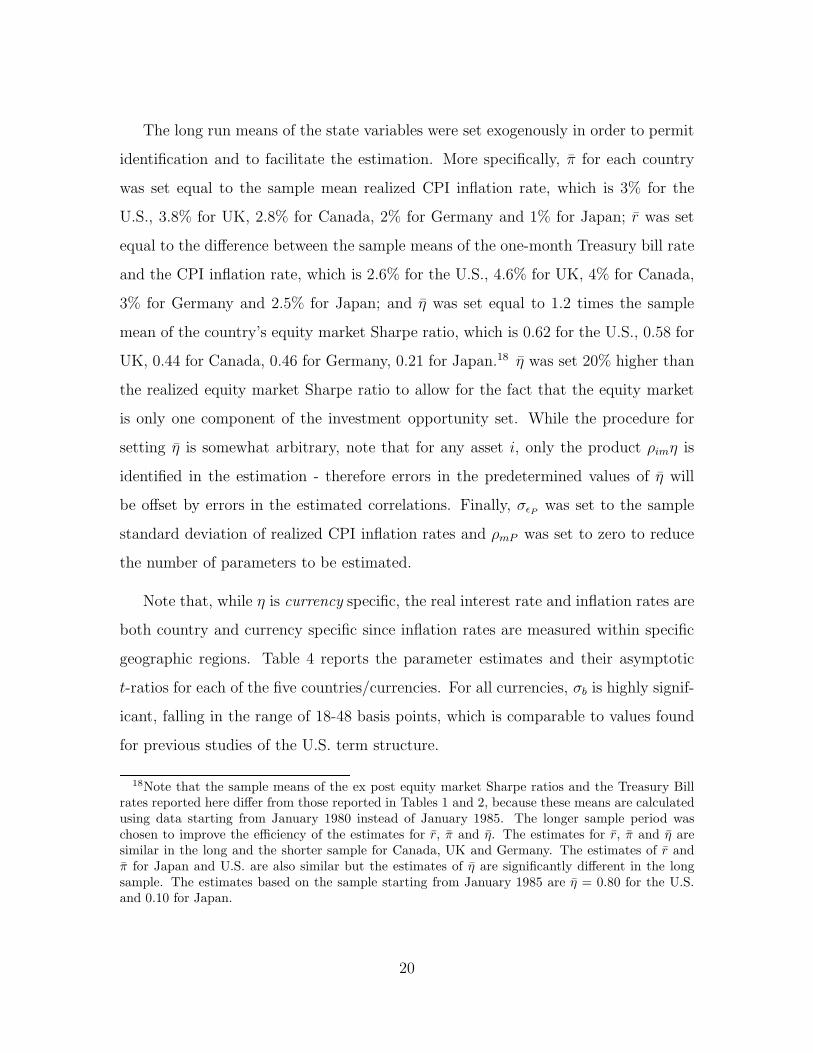
The long run means of the state variables were set exogenously in order to permit

identification and to facilitate the estimation. More specifically, π for each country

was set equal to the sample mean realized CPI inflation rate, which is 3% for the

U.S., 3.8% for UK, 2.8% for Canada, 2% for Germany and 1% for Japan; r was set

equal to the difference between the sample means of the one-month Treasury bill rate

and the CPI inflation rate, which is 2.6% for the U.S., 4.6% for UK, 4% for Canada,

3% for Germany and 2.5% for Japan; and η was set equal to 1.2 times the sample

mean of the country’s equity market Sharpe ratio, which is 0.62 for the U.S., 0.58 for

UK, 0.44 for Canada, 0.46 for Germany, 0.21 for Japan.18 η was set 20% higher than

the realized equity market Sharpe ratio to allow for the fact that the equity market

is only one component of the investment opportunity set. While the procedure for

setting η is somewhat arbitrary, note that for any asset i, only the product ρimη is

identified in the estimation - therefore errors in the predetermined values of η will

be offset by errors in the estimated correlations. Finally, σεPwas set to the sample

standard deviation of realized CPI inflation rates and ρmP was set to zero to reduce

the number of parameters to be estimated.

Note that, while η is currency specific, the real interest rate and inflation rates are

both country and currency specific since inflation rates are measured within specific

geographic regions. Table 4 reports the parameter estimates and their asymptotic

t-ratios for each of the five countries/currencies. For all currencies, σb is highly signif-

icant, falling in the range of 18-48 basis points, which is comparable to values found

for previous studies of the U.S. term structure.

18Note that the sample means of the ex post equity market Sharpe ratios and the Treasury Billrates reported here differ from those reported in Tables 1 and 2, because these means are calculatedusing data starting from January 1980 instead of January 1985. The longer sample period waschosen to improve the efficiency of the estimates for r, π and η. The estimates for r, π and η aresimilar in the long and the shorter sample for Canada, UK and Germany. The estimates of r andπ for Japan and U.S. are also similar but the estimates of η are significantly different in the longsample. The estimates based on the sample starting from January 1985 are η = 0.80 for the U.S.and 0.10 for Japan.

20

For all countries except the U.S., σr, the volatility of the real interest rate inno-

vation, is in the range of 63-92 basis points per year; for the U.S. on the other hand

it is 277 basis points. The high volatility of r in the U.S. is offset by strong mean

reversion: the estimate of κr is more than twice as high for the U.S. as for the next

highest country, the U.K., and implies a half life for innovations of about 2.4 years,

as compared with almost 5 years in the U.K., almost 6 years in Canada, and more

than 10 years in Germany where the mean reversion parameter is not significant. As

we shall see below, there is evidence of mean reversion in the estimates of r for all

these countries. For Japan on the other hand the estimated value of r declines fairly

steadily from 1990 so that there is little evidence of mean reversion in this sample

period. It is not surprising then to find that the estimate of κr is close to zero and

insignificant; the Ornstein-Uhlenbeck assumption clearly fails to capture the behavior

of the real interest rate in Japan during this sample period. The estimated correlation

between innovations in the real interest rate and the pricing kernel, ρrm, is negative

and highly significant for all five currencies, so that for all there is a significant real

interest rate risk premium and long term bonds command a positive premium.

The volatility of innovations in the expected inflation rate, σπ, is highly signifi-

cant except for Japan, ranging from 40 basis points in Japan to 115 basis points in

Germany. The estimates of the mean reversion parameter for expected inflation, κπ,

are very small and insignificant for the Anglo-Saxon countries, U.S., UK and Canada,

but are much larger and significant in Germany and Japan. The estimates for the

Anglo-Saxon countries are consistent with previous findings that expected inflation

follows close to a random walk. We place little weight on the estimate for Japan

since it is clear that expected inflation, like the real interest rate, does not conform

to the O-U assumption underlying the estimation during this sample period. Finally,

ρπm is not significant for any country so that there is no evidence of a risk premium

associated with expected inflation.

The point estimate of the volatility of the maximum Sharpe ratio process, ση, is

21

in the range of 0.19 to 0.28 for all currencies except the Japanese Yen (JY) where

it is only 0.06 - this may reflect the generally poor fit of the model to Yen yields

during this sample period, or it may reflect the fact that we have chosen a low value

of the scaling parameter η for Japan. The point estimate is highly significant only

for the Pound (BP); the lack of significance for the USD is a little surprising, since

the stochastic nature of risk premia in the U.S. has been widely documented, and

Brennan, Wang and Xia (2003) and Brennan and Xia (2003) report estimates of ση

for the periods 1952-2000 and 1983-2000 that are highly significant. Just as for the

real interest rate, the estimate of the mean-reversion parameter, κη, is highest for the

USD and lowest for the DM and JY where the model does not fit so well.19 The half

life of innovations in η is almost 9.5 years for the Canadian dollar (CAD), around 6.7

years for the BP, and about 2.4 years for the USD.

Finally, ρηm, is significant and in the range of 0.8 to 0.92 for all currencies except

the JY for which, as mentioned, the model does not fit well. It is also interesting to

note that, with the exception of the JY for which ρηm is negative and insignificant,

the signs of ρrm and ρηm are opposite and are consistent across currencies, so that

the risk premia for these fundamental investment opportunity set risks are priced in

a consistent fashion across currencies. However, the absolute values of the estimated

correlations ρrm and ρηm seem high for most countries, which suggests that we may

have underestimated the levels of the pricing kernel volatilities by setting η too low.

In summary, the estimation results display an encouraging consistency across cur-

rencies/countries except for Japan and the Yen where the post-bubble economy has

not conformed well to the model assumptions about the real interest rate or inflation.

Table 5 reports summary statistics on the estimated state variables, r, π and η,

that are obtained from the Kalman filter for each of the countries/currencies. Note

first that the sample mean of a state variable estimate reported in Table 5 may

19The Maximized likelihood is lowest for these two countries.

22

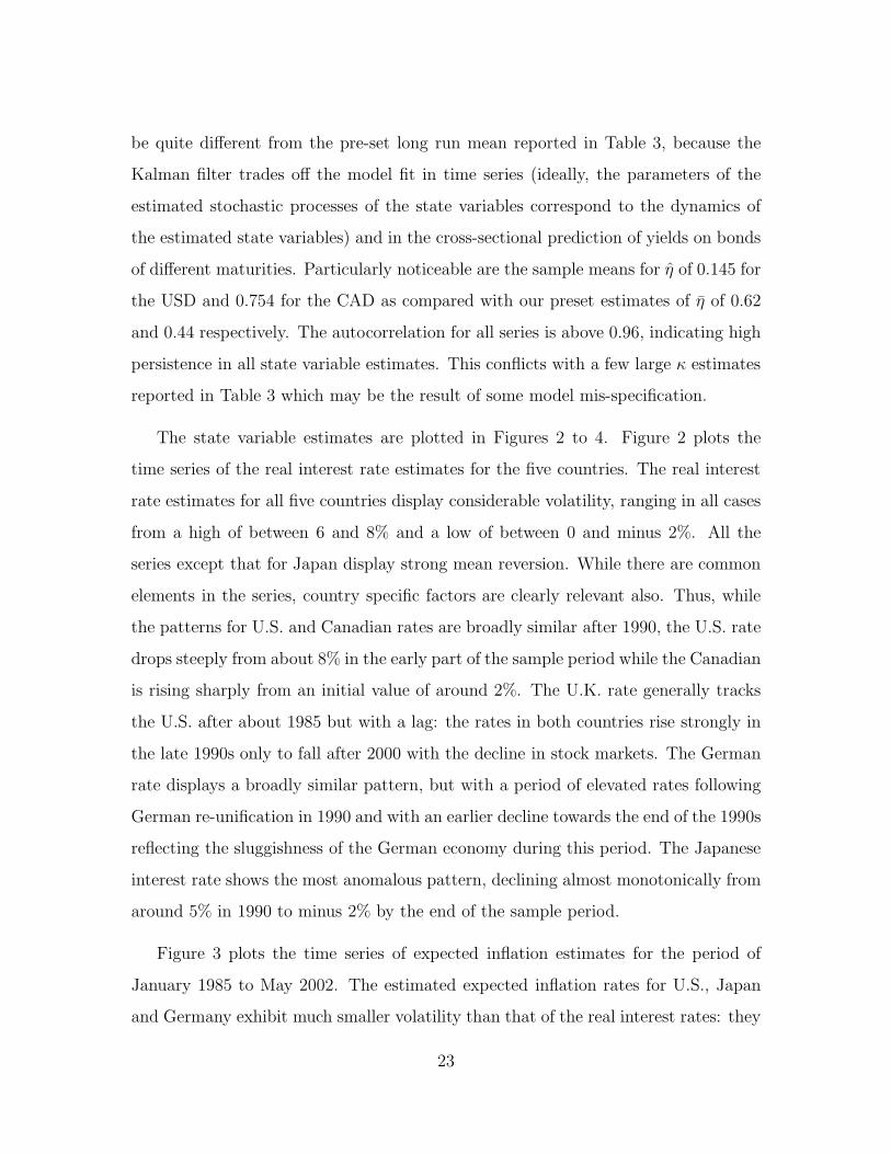
be quite different from the pre-set long run mean reported in Table 3, because the

Kalman filter trades off the model fit in time series (ideally, the parameters of the

estimated stochastic processes of the state variables correspond to the dynamics of

the estimated state variables) and in the cross-sectional prediction of yields on bonds

of different maturities. Particularly noticeable are the sample means for η of 0.145 for

the USD and 0.754 for the CAD as compared with our preset estimates of η of 0.62

and 0.44 respectively. The autocorrelation for all series is above 0.96, indicating high

persistence in all state variable estimates. This conflicts with a few large κ estimates

reported in Table 3 which may be the result of some model mis-specification.

The state variable estimates are plotted in Figures 2 to 4. Figure 2 plots the

time series of the real interest rate estimates for the five countries. The real interest

rate estimates for all five countries display considerable volatility, ranging in all cases

from a high of between 6 and 8% and a low of between 0 and minus 2%. All the

series except that for Japan display strong mean reversion. While there are common

elements in the series, country specific factors are clearly relevant also. Thus, while

the patterns for U.S. and Canadian rates are broadly similar after 1990, the U.S. rate

drops steeply from about 8% in the early part of the sample period while the Canadian

is rising sharply from an initial value of around 2%. The U.K. rate generally tracks

the U.S. after about 1985 but with a lag: the rates in both countries rise strongly in

the late 1990s only to fall after 2000 with the decline in stock markets. The German

rate displays a broadly similar pattern, but with a period of elevated rates following

German re-unification in 1990 and with an earlier decline towards the end of the 1990s

reflecting the sluggishness of the German economy during this period. The Japanese

interest rate shows the most anomalous pattern, declining almost monotonically from

around 5% in 1990 to minus 2% by the end of the sample period.

Figure 3 plots the time series of expected inflation estimates for the period of

January 1985 to May 2002. The estimated expected inflation rates for U.S., Japan

and Germany exhibit much smaller volatility than that of the real interest rates: they

23

vary only from around 0.5% to around 4%. On the other hand, the UK rate moves

around in a tight range between 3% to 6% until 1997 when it falls rapidly to below

0 and then increases slightly; the estimate for Canada has long swings in the much

larger range of 0.5% to over 7%.

Figure 4 plots the Sharpe ratio estimates. The Sharpe ratios for the USD, BP,

and DM all reach their lows at the peak of the stock market boom in the 1999-2000

period, the USD decline starting around 1993, the BP around 1995, and the DM

around 1996. The ratios for all three currencies recover rapidly towards the end of

the sample period. The CAD and JY ratios also decline in the second half of the

1990s, but not so dramatically as in the other three countries, and for both CAD and

JY the lows (in both cases below zero) are reached in 1990. In the first half of the

1990s Sharpe ratios for all currencies are generally increasing. Finally, in contrast

to the unrelated movements in the real interest rates in Canada and the U.S. up to

1990, their Sharpe ratios display strong comovement, initially rising sharply and then

entering a long period of decline from 1986 to 1990.

To explore further the relation between the state variables for the different coun-

tries/currencies vector autoregressions were run separately for r, π, and η and the

results are reported in Table 6,20 which also reports the correlation matrix of the

estimated state variable innovations. Table 6A shows that feedback between the real

interest rates in the different countries is primarily limited to the U.S.-Canada and

U.K.-Germany country pairs. While the Canadian interest rate has no influence on

the U.S. rate, the U.S. rate acts like the target towards which the Canadian rate ad-

justs: the VAR coefficients imply that the expected monthly change in the Canadian

rate can be written approximately as 0.05 (rUS − rCAN). Similarly the change in the

German rate can be written approximately as 0.05 (rUK − rGER). On the other hand,

the influence of the German rate appears anomalous since it enters with a negative

20Strictly speaking, the VAR specification is inconsistent with the parsimonious Ornstein-Uhlenbeck assumption that we have made about the state variable dynamics.

24

coefficient in the regressions of all the other countries, and the coefficient is significant

for Canada and the U.K. We suspect that this is the spurious result of the coinci-

dence of the German re-unification boom and fiscal deficit with economic downturns

in the other countries. The correlations between the real interest rate innovations in

all countries are positive as seen in Panel II, the highest correlations being between

Canada and the U.S. (0.48) and Germany and the U.K. (0.44); the next highest cor-

relation is between Germany and Japan (0.38). These results are consistent with

the hypothesis that geographical proximity and trade relations are associated with

common shocks to real interest rates.

The (real) pricing kernel volatilities or ‘Sharpe ratios’21 show a more complicated

pattern. First, as shown in Table 6B the estimated USD Sharpe ratio is significantly

influenced by the lagged CAD Sharpe ratio, though the weight on this variable is

very small and negative. The CAD Sharpe ratio is influenced strongly by the lagged

value of both the USD and JY ratios. The DM Sharpe ratio is influenced strongly

by the lagged BP ratio and negatively by the JY ratio. As with the real interest rate,

the DM Sharpe ratio has a small negative influence on those of the other currencies

(excluding the USD.). However, the correlations between the Sharpe ratio innovations

for all currencies are positive, once again the highest correlations being between the

CAD and USD ratios (0.54) and between the DM and BP ratios (0.41)., all other

correlations being considerably smaller. The high correlations for the Sharpe ratio

innovations for CAD and USD and for DM and BP are consistent with the much

lower levels of exchange risk between these currencies: as seen in Table 3 these two

exchange rates have the lowest volatilities.

Table 6C reports the results for expected inflation rates. The most striking aspect

of the VAR coefficients is the strong dependence of Canadian (expected) inflation

on (expected) inflation in the other countries, especially the U.S. and Japan. U.S.

21The (absolute value of) the volatility of the pricing kernel is equal to the maximum Sharpe ratiofor returns in a given currency.

25

inflation is moderately affected by inflation in all countries except Germany and

the coefficient for Canada is negative. The correlations between the innovations in

expected inflation are much smaller than for the other series except between the three

Anglo-Saxon countries where the correlations range from 0.46 to 0.63.

Overall, we have found strong links between Canada and the U.S. and between

Germany and the U.K. for the real variables, the interest rate and the Sharpe ratio,

and between the three Anglo-Saxon countries for expected inflation.

6 Empirical Evidence on Capital Market Integra-

tion

In this section, we carry out a direct test of market integration using our esti-

mates of the pricing kernel volatilities. We first examine whether the pricing kernel

volatilities are linearly related as prescribed by the model, and then test whether the

uncovered currency return, defined as the realized spot rate appreciation minus the

forward premium, is related to the pricing kernel volatilities.

6.1 Volatility of the Domestic and Foreign Real Pricing Ker-nels

In this section we consider how well the restriction implied by condition (23) is

satisfied in the data:

η∗ =ρSm

ρSm∗η − σS

ρSm∗+

σP ρSP − σP ∗ρSP ∗

ρSm∗.

A simple regression of η∗ on η will yield spurious results since η∗, and η are highly

autocorrelated.22 Therefore we report the results under two different estimations, one

22See Chapter 18 of Hamilton (1994) for detailed discussions. Roll and Yan (2000) discuss thisproblem in the context of the forward premium puzzle.

26

using first differences, and the second a cointegrating regression approach. We treat

σS as a constant for some of the regressions and also include it as a variable using

data on the implied volatility of the exchange rate when they are available.

The first difference regression with constant σS is specified as:

η∗t+1 − η∗

t = a0 + a1 (ηt+1 − ηt) + ε, (30)

where, under the null hypothesis, a0 = 0 and a1 6= 0. If σS is stochastic, then the

first difference regression is given by:

η∗t+1 − η∗

t = a0 + a1 (ηt+1 − ηt) + a2 (σS,t+1 − σS,t) + ε, (31)

where a0 = 0, a1 6= 0, and a2 6= 0 under the null.

Table 7 reports the first difference regression results for the whole sample in the

first three columns. Consistent with the null hypothesis, the estimates of a0 are all

small in magnitude and statistically insignificant, while the estimate of a1 is highly

significant for all except the USD/JY regressions. The positive sign of the coefficient

a1 implies that the correlation of the exchange rate change with both pricing kernels

has the same sign. The regressions have R2 of between 5 and 19% (except for the

USD/JY, DM/JY and JY/USD regressions).

Table 7A reports the results when σS is added to the first difference regression.

Since the implied exchange rate volatility is available only for all currencies against

the USD and for the BP-DM, and DM-JY exchange rates, the sample is reduced to

regressions that include the USD η as either dependent or independent variable or the

BP-DM and DM-JY pairs, and the sample period is restricted to the period beginning

October 1994. When σS is included the estimated value of a1 increases in all cases,

and all estimates except for the DM-JY pair are positive and significantly different

from zero. As before, regressions involving JY have small R2 and insignificant or

only marginally significant estimates of a1. The R2 of other regressions increase to

27

between 24 and 56 % while the R2 in Table 7 were all less than 20% and most were

less than 10%. However, it is not the inclusion of σS but the reduced sample period

that accounts for the improved results, for the estimated coefficient of the change in

the exchange rate is nowhere significant. Therefore, regression (30) was repeated for

all currencies for two sub-periods and the results are reported in the second and third

blocks of Table 7. The first sub-period is from January 1985 to September 1994, and

the second sub-period, consistent with the sample in Table 7A, is from October 1994

to May 2002.

The first sub-period generally has low R2 (all less than 10%) and only three out

of twenty currency pairs yield a significant (at 5% level) estimate of a1. In contrast,

the estimates of a1 are highly significant in the second sub-period except for three

currency pairs, all of which involve the JY. The goodness of fit is broadly improved

in the second sub-period, the R2’s all being above 20% except for those involving

JY. For example, the R2 for the DM-USD pair improves from 0 to around 27% while

the DM-BP pair moves from only 5% to over 40%. Even for currency pairs that

include JY, the goodness of fit also increases. For example, the R2 for the BP-JY

pair increases from only 1.8% to over 16%. The much stronger results in the second

sub-period are consistent with increasing capital market integration over time. For

the whole sample, as well as for the two sub-periods, the currency pairs that include

JY always have the weakest results. This is consistent with Brandt, Cochrane and

Santa-Clara (2002), who report that their risk sharing index is the lowest for Japan.

In addition to the first difference regression, we examine the relation given in (23)

directly, using a cointegration regression since both η and η∗ are highly persistent. Ta-

ble 8 reports the cointegration coefficient estimates for the whole sample and the two

sub-periods. The cointegration coefficient estimates are generally larger in absolute

values than their counterparts reported in Table 7 and eleven, twelve, and fifteen out

of twenty pairs have significant slope estimates for, respectively, the whole, the first

and the second sub-periods. The sign of the significantly estimated slope coefficient

28

is opposite to that in Table 7 for eight country pairs for the whole sample, but it is

broadly consistent between the two tables for the second sub-period.

Table 8A reports the cointegration regression results when the implied foreign

exchange volatility, σS, is treated as a stochastic variable. In contrast to the results

reported in Table 7A, the cointegration coefficients for σS, c2, are now all highly sig-

nificant except for the BP-DM pair, and the magnitude of c2 is comparable to that

of c1, the estimated coefficient of η. Nine out of twelve pairs have highly significant

values of c1 while the first difference regression also yielded nine out of twelve signif-

icant estimates for the coefficient of η. Note that the cointegration results may be

less reliable because of the short sample period (November 1994 to May 2002). The

results involving the DM may be even less reliable because of the transition from DM

to Euro in January 1999.

6.2 Exchange Rate Risk Premia and Currency Sharpe Ratios

Finally we examine whether time-variation in exchange rate risk premia is related

to time-variation in the Sharpe ratios associated with the individual currencies as

our model predicts. Equation (19) relates the expected rate of currency appreciation,

Et ≡ (E[St+1] − St) /St, to the interest rate differential, R∗t − Rt and the domestic

Sharpe ratio, η. Since covered interest rate parity implies that the interest rate

differential is equal to the forward premium, Rt −R∗t = (Ft − St) /St, where Ft is the

one period forward exchange rate at time t, equation (19) implies that:

E[St+1] − St

St

=Ft − St

St

+ ησSρSm + σSσP ρSP ,

or equivalently,E[St+1] − Ft

St= ησSρSm + σSσP ρSP

where St (Ft) is the foreign spot (one-period forward) exchange rate at time t denom-

inated as the domestic currencies per unit of foreign currency and η is the domestic

29

Sharpe ratio. This motivates the following regression under the assumption that σS

is constant:

St+1 − Ft

St

= a0 + a1η + ε (32)

with H0 : a1 6= 0.

We first carry out the simple OLS regression to examine equation (32) and report

the results in Table 9. The results are generally disappointing: the adjusted R2’s are

quite low, and only four out of twenty exchange rates yield significant estimates for

a1. One interesting observation is that a1 is generally significant when ηUS is on the

right hand side of equation (32). In addition, the BP-DM regression is significant.

Although the unit-root null hypothesis is strongly rejected for the spot rate appre-

ciation, (St+1 − St) /St, and the uncovered currency return, (St+1 − Ft) /St, for all

country pairs,23 η is highly persistent with close-to-unit root autocorrelations. It is

possible that the unobservable ex ante uncovered currency return is persistent and has

close-to-unit root, but the i.i.d. measurement errors in the realized currency return

is so large that the persistence in the true variable is obscured, as argued by Ferson

et. al. (2003). Therefore, we re-estimate the relation (32) using the cointegration

approach.

Table 10 reports the results when a constant σS is assumed. The estimated co-

efficient of η is significant is seven out of the twenty regressions - interestingly, the

coefficient is always significant when the relevant independent variable is the USD

Sharpe ratio. In addition, the DM Sharpe ratio is significant for the USD-DM and

CAD-DM regressions while the CAD Sharpe ratio is significant for the DM-CAD

regression. For most of the other currencies the coefficient of the Sharpe ratio is

positive but not significant. Thus foreign exchange risk premia move with the premia

23The forward premium or the uncovered currency return in general does not have a close-to-unit-root autocorrelation coefficient: the highest among all country pairs is only 0.82. Roll and Yan(2000) find non-stationarity in the forward premium, (Ft − St) /St, for a different sample period.

30

on other USD denominated assets, but they do not appear to be strongly influenced

by risk premia on assets denominated in other currencies. This may reflect the pre-

dominance of the USD as a reserve currency. The OLS and cointegration regressions

were also repeated using Euro-currency one-month interest rate differentials instead

of the forward premium, with virtually identical results.

However, if σS is not constant, then equation(32) will be mis-specified. Therefore,

we also repeat the analysis allowing for a time varying σS by estimating the co-

integrating regression:

St+1 − Ft

St= c0 + c1ησS + c2σS + ε. (33)

with H0 : c0 = 0, c1 6= 0.

As before, this restricts the sample to currency pairs that include the USD plus two

DM exchange rates. Table 10A reports the results for all exchange rates relative to the

USD and the DM-JY and DM-BP rates for October 1994 to May 2002, the period

for which implied volatility data are available. The coefficient of σS is significant

in ten out of the twelve regressions for which a co-integrating regression could be

estimated - the risk premia are clearly related to risk.24 The estimated coefficient

of the Sharpe ratio, c1, is always significant for the BP-DM and USD-DM pairs no

matter whether the relevant independent variable is the USD, the BP, or the DM

Sharpe ratio. On the other hand, c1 is significant for the CAD-USD and BP-USD

regressions only when the independent variable is the USD Sharpe ratio. c1 is also

significant in the DM-JY regression where the independent variable is the JY Sharpe

ratio. However, this variable is not significant in the USD-JY regression. In general,

the results are slightly strengthened by allowing for stochastic σS .

It is possible that the influence of η is obscured by its multiplication in regression

24Brandt and Santa-Clara (2002) have also found that the implied volatility of the exchange rateis significant in explaining the risk premium for the USD-BP and USD-DM exchange rates.

31

(33) by σS , which also enters as an independent variable. Therefore we also estimate

the following equation which separates the influence of η from that of σS:

St+1 − Ft

St

= c0 + c1η + c2σS + ε. (34)

The results, which are reported in Table 10B, are broadly consistent with those re-

ported in Table 10A.

These results, taken together, show that, consistent with a rational model, time

variation in foreign exchange risk premia may be attributed to both changing risk-

return trade-offs available in domestic capital markets and to the changing level of

exchange rate volatility. While it is somewhat discouraging that neither the Canadian

nor UK Sharpe ratios are significantly related to the dollar risk premium, this may

possibly be accounted for by the shortness of the period for which exchange rate

volatility data can be calculated.

7 Conclusion

We have shown that in integrated capital markets in which there are no arbitrage

opportunities there exists a simple relation between the volatilities of the (minimum

variance) pricing kernels (or maximum Sharpe ratios) for returns denominated in dif-

ferent currencies and the volatility of the exchange rates between them. We have also

shown that, for a given exchange rate volatility, the foreign exchange risk premium is

a linear function of the maximum Sharpe ratio. Then, using the parsimonious three-

factor essentially affine model of the pricing kernel proposed by Brennan, Wang and

Xia (2003), we have estimated real interest rates, expected inflation and the volatility

of the pricing kernels (maximum Sharpe ratios) for five major currencies from panel

data on zero coupon bond yields and inflation.

To explore the inter-relations between the state variables for different currencies

32

we ran vector autoregressions for each of the state variables across currencies. The

innovations in both the real interest rates and the Sharpe ratios were found to be

positively correlated across all currencies, the strongest correlations being for the

CAD/USD and DM/BP pairs. The innovations in expected inflation were much less

correlated, the highest correlations being between CAD, USD and BP. The CAD real

interest rate and Sharpe ratio were found to be strongly influenced by the lagged

values of the corresponding USD variables; other significant lag relations were found

between the CAD Sharpe ratio and the lagged JY Sharpe ratio and between the DM

Sharpe ratio and the lagged BP ratio.

The relations between Sharpe ratios for different currencies were further explored

by regressing changes in one ratio on changes in another and by co-integrating re-

gressions. The first difference regressions have R2 of between 5 and 19% (except for

the USD/JY, DM/JY and JY/USD regressions for which the R2 are lower). The

point estimate of the regression coefficient is close to its theoretical value of unity

for CAD/USD, CAD/JY, and DM/JY. Despite the fact that the Sharpe ratio is

identified only up to a scalar multiple by the model, several of the estimates of the

regression coefficient are too far from their theoretical value of unity to be explicable

in terms of an inappropriate scaling for particular currencies; in particular, all of the

regressions in which the JY η is the dependent variable have coefficient estimates

below 0.1. Regressions for the post October 1994 period yielded higher R2 and the

regression coefficient was significant in 18 out of 20 regressions. The results were

generally unchanged by the inclusion of the change in the exchange rate volatility

in the regression. Cointegrating regressions between pairs of η’s confirmed the first

difference regression results: for the post 1994 period 16 out of 20 coefficients were

significant. When the exchange rate volatility was added to the co-integrating regres-

sion its coefficient was significant in 8 out of 12 regressions as was the coefficient of

η. The weakest relations were observed between changes in the JY η and the η’s of

other currencies.

33

Finally, the uncovered return on foreign currency investment was regressed on the

domestic Sharpe ratio for each of the currencies. These results also are stronger for

the post 1994 period. For this period, when the volatility of the exchange rate is

included in the regression the returns were found to be significantly related to the

volatility of the exchange rate in nine out of the twelve regressions, while the Sharpe

ratio was significant in seven out of the twelve regressions. The strongest results were

for the USD Sharpe ratio which was significant in three out of four regressions (not

in the JY regression), while the JY Sharpe ratio was significant in explaining risk

premia on investments denominated in DM (but not USD) and the DM Sharpe ratio

was significant in explaining returns on investments in BP and USD (but not JY).

The BP Sharpe ratio was significant for the returns on investments denominated

in DM but not USD. Thus uncovered returns on foreign currency investment are

generally related both to the risk of that investment as measured by the volatility of

the exchange rate and to the level of risk premia prevailing in the domestic capital

market as measured by the domestic Sharpe ratio. The influence of the domestic

market Sharpe ratio is weakest for foreign investments in JY and in USD.

Overall, the results are consistent with a high degree of integration in international

capital markets in the period since 1994, except possibly for the JY market whose η

was little related to those of other currencies and whose currency returns denominated

in other currencies were little related to the η’s of those currencies. This may reflect

the continuing importance of government intervention in the JY market even in the

post 1994 period, and the poor quality of the state variable estimates derived from

the Japanese bond market.

34

References

Ahn, Dong-Hyun, 1997, Generalized squared-autoregressive-independent-variable

nominal term structural model, unpublished working paper, University of North Car-

olina.

Adler, M., and B. Dumas, 1993, International Portfolio Choice and Corporate

Finance: A Synthesis, The Journal of Finance 38, 925-984.

Babbs, Simon H., and K. Ben Nowman, 1999, Kalman filtering of generalized

Vasicek term structure models, Journal of Financial and Quantitative Analysis 34,

115-130.

Backus, D., A. Gregory, and C. Telmer, 1993, Accounting for Forward Rates in

Markets for Foreign Currency, The Journal of Finance 48, 1887-1908.

Backus, D., S. Foresi, and C. Telmer, 2001, Affine Term Structure Models and the

Forward Premium Anomaly, Journal of Finance 56, 279-304.

Bansal, R., 1997, An Exploration of the Forward Premium Puzzle in Currency

Markets, Review of Financial Studies 10, 369-403.

Bekaert, G., 1995, The Time Variation of Expected Returns and Volatility in

Foreign Exchange Markets, Journal of Business and Economic Statistics 13, 397-408.

Bekaert, G., 1996, The Time-variation of Risk and Return in Foreign Exchange

Markets: A General Equilibrium Perspective, Review of Financial Studies 9, 427-470.

Bekaert, G., and C. Harvey, 1995, Time-Varying World Market Integration, The

Journal of Finance 50, 403-444.

Bliss, R. R., Testing Term Structure Estimation Methods, Advances in Futures

and Option Research 9, 197-231.

Brandt, M., and P. Santa-Clara, 2002, Simulated likelihood estimation of diffu-

35

sions with an application to exchange rate dynamics in incomplete markets, Journal

of Financial Economics 63, 161-210.

Brandt, M., J. Cochrane, and P. Santa-Clara, 2003, International risk sharing is

better than you think (or exchange rates are much too smooth), unpublished manu-

script, UCLA.

Brennan, M.J., and H.H. Cao, 1997, International Portfolio Investment Flows,

The Journal of Finance 52, 1851-1880.

Brennan, M.J., H.H. Cao, N. Strong and X. Xu, 2003, The Dynamics of Interna-

tional Equity Market Expectations, Working Paper, UCLA.

Brennan, Michael J., and Yihong Xia, 2002, Dynamic asset allocation under in-

flation, Journal of Finance 57, 1201-1238.

Brennan, M.J., and Y. Xia, 2003, Risk and Valuation under an Intertemporal

Capital Asset Pricing Model, Working Paper, University of Pennsylvania.

Brennan, M.J., A. Wang, and Y. Xia, 2003, Estimation and Test a Simple In-

tertemporal Capital Asset Pricing Model, Working paper, University of Pennsylvania.

Cappiello, L., O. Castren, and J. Jaaskela, 2003, Measuring the Euro Exchange

Rate Risk Premium: the Conditional International CAPM Approach, Working paper,

European Central Bank.

Cumby, R., 1988, Is It Risk? Explaining Deviations from Uncovered Interest

Parity, Journal of Monetary Economics 22, 279-299.

De Santis, G., and B. Gerard, 1997, International Asset Pricing and Portfolio

Diversification with Time-Varying Risk, The Journal of Finance 52, 1881-1912.

De Santis, G., and B. Gerard, 1998, How Big is the Premium for Currency Risk?,

Journal of Financial Economics 49, 375-412.

Domowitz, I., and C. Hakkio, 1985, Conditional Variance and the Risk Premium

36

in the Foreign Exchange Market, Journal of International Economics 19, 47-66.

Duffee, G., 2002, Term Premia and Interest Rate Forecasts in Affine Models,

Journal of Finance 57, 405-443.

Dumas, B., and B. Solnik, 1995, The World Price of Foreign Exchange Risk, The

Journal of Finance 50, 445-479.

Engel, C., 1996, The Forward Discount Anomaly and the Risk Premium: A Survey

of Recent Evidence, Journal of Empirical Finance 3, 123-192.

Engsted, T., and C. Tanggaard, 2002, The Relation between Asset Returns and

Inflation at Short and Long Horizons, Journal of International Financial Markets,

Institutions and Money 12, 101-118.

Fama, E., 1984, Forward and Spot Exchange Rates, Journal of Monetary Eco-

nomics 14, 319-338.

Ferson, W., and C. Harvey, 1994, Sources of Risk and Expected Returns in Global

Equity Markets, Journal of Banking and Finance 18, 775-803.

Ferson, W., Timothy Simin, and Sergei Sarkissian, 2003, Spurious regressions in

Financial Economics?, The Journal of Finance, forthcoming.

Giovannini, A., and P. Jorion, 1989, The Time-Variation of Risk and Return in

the Foreign Exchange and Stock Markets, The Journal of Finance 44, 307-325.

Hamilton, J., 1994, Time Series Analysis, (Princeton University Press, Princeton,

New Jersey).

Hansen, L., and R. Hodrick, 1983, Risk Averse Speculation in the Forward Foreign

Exchange Market, in J. A. Frankel, ed.: Exchange Rates and International Macroeco-

nomics (University of Chicago Press, Chicago, IL).

Harvey, C., 1991, The World Price of Covariance Risk, The Journal of Finance

46, 111-157.

37

Hollifield, B., and R. Uppal, 1997, An Examination of Uncovered Interest Rate

Parity in Segmented International Commodity Markets, The Journal of Finance) 52,

2145-2170.

Huang, C-f., 1985, Information Structure and Equilibrium Asset Prices, Journal

of Economic Theory 31, 33-71.

Ilmanen, A., 1995, Time-Varying Expected Returns in International Bond Mar-

kets, The Journal of Finance 50, 481-506.

Jorion, P., 1995, Predicting Volatility in the Foreign Exchange Market, The Jour-

nal of Finance 50, 507-528.

Korajczyk, R., and C. Viallet, 1990, An Empirical Investigation of International

Asset Pricing, Review of Financial Studies 2, 53-85.

Lewis, K., 1995, Puzzles in International Financial Markets, in G. M. Grossman

and K. Rogeff eds Handbook of International Economics, Vol. 3, Chapter 13, Ams-

terdam, Elsevier.

Litzenberger, R.H., and J. Rolfo, 1984, An International Study of Tax Effects on

Government Bonds Journal of Finance 39, 1-22.

McCrown, J. R., 2001, Yield Curves and International Equity Returns, Journal

of Banking and Finance 25, 767-788.

McCulloch, J.H., 1975, The Tax Adjusted Yield Curves, The Journal of Finance

30, 811-830.

Meredith, G., and M. Chinn, 1998, Long-Horizon Uncovered Interest Rate Parity,

NBER Working Paper #6797.

Nielsen, Lars Tyge, and Jesus Saa-Requejo, 1993, Exchange Rate and term struc-

ture dynamics and the pricing of derivative securities, working paper, INSEAD.

Portes, R., H. Rey, and Y. Oh, 2001, Information and Capital Flows, European

38

Economic Review 45, 783–796.

Robotti, C., 2001, The Price of Inflation and Foreign Exchange Risk in Interna-

tional Equity Markets, Working Paper 2001-26, Federal Reserve Bank of Atlanta.

Roll, R., and S. Yan, 2000, An Explanation of the Forward Premium ”Puzzle”,

European Financial Management 6, 121-148.

Saa-Requejo, J., 1993, The dynamics and the term structure of risk premium in

foreign exchange market, working paper, INSEAD.

Tzavalis, E., and M. R. Wickens, 1996, Forecasting Inflation from the Term Struc-

ture, Journal of Empirical Finance 3, 103-122.

39

Table 1

Summary Statistics of Fitted Zero-Coupon Constant Maturity Bond Yields

This table reports sample summary statistics for the fitted zero-coupon constant maturity bond yields. The

bond yields are estimated from government coupon bonds using a cubic spline. The raw government coupon bond

data are collected from Datastream. The sample is from January 1985 to May 2002

1. The United States

Bond Yield Maturities CPI ExcessSecurities 0.5 1 2 3 5 7 10 Infl Mkt Ret.Mean (% per year) 6.07 6.14 6.27 6.41 6.69 6.96 7.41 3.08 9.97Std. Dev. (% per year) 1.64 1.59 1.58 1.61 1.53 1.19 0.82 0.77 15.04Autocorrelation 0.98 0.98 0.98 0.98 0.98 0.98 0.98 0.34 0.00Correlation0.5 1.0 0.99 0.92 0.84 0.73 0.74 0.74 0.26 -0.031 1.0 0.97 0.91 0.81 0.81 0.72 0.29 -0.022 1.0 0.98 0.93 0.88 0.67 0.27 0.013 1.0 0.98 0.92 0.62 0.26 0.035 1.0 0.95 0.61 0.25 0.027 1.0 0.80 0.28 -0.0510 1.0 0.29 -0.17Infl 1.0 -0.09

2. Canada

Bond Yield Maturities CPI ExcessSecurities 0.5 1 2 3 5 7 10 Infl Mkt Ret.Mean (% per year) 6.99 7.09 7.18 7.45 7.70 7.84 8.01 2.78 5.50Std. Dev. (% per year) 2.53 2.43 2.26 2.14 1.99 1.88 1.82 1.13 14.84Autocorrelation 0.98 0.98 0.98 0.98 0.98 0.98 0.98 0.09 0.09Correlation0.5 1.0 0.998 0.98 0.96 0.89 0.87 0.87 0.32 -0.161 1.0 0.99 0.97 0.91 0.90 0.89 0.32 -0.162 1.0 0.99 0.96 0.94 0.92 0.32 -0.153 1.0 0.98 0.97 0.94 0.32 -0.155 1.0 0.99 0.96 0.30 -0.137 1.0 0.99 0.28 -0.1210 1.0 0.25 -0.12Infl 1.0 -0.01

40

Table 1 (continued)

3. The United Kingdom (from Bank of England)

Bond Yield Maturities CPI ExcessSecurities 1 2 3 5 7 10 15 Infl Mkt Ret.Mean (% per year) 8.02 8.03 8.06 8.11 8.14 8.10 7.88 3.80 6.16Std. Dev. (% per year) 2.65 2.35 2.21 2.13 2.12 2.10 1.97 1.63 16.73Autocorrelation 0.99 0.98 0.98 0.98 0.98 0.99 0.99 0.24 0.03Correlation1 1.0 0.99 0.97 0.93 0.90 0.87 0.80 0.36 -0.032 1.0 0.99 0.97 0.95 0.92 0.86 0.36 -0.043 1.0 0.99 0.98 0.95 0.90 0.35 -0.045 1.0 0.99 0.98 0.95 0.34 -0.037 1.0 0.99 0.97 0.32 -0.0310 1.0 0.99 0.30 -0.0115 1.0 0.27 0.01Infl 1.0 -0.09

4. Germany

Bond Yield Maturities CPI ExcessSecurities 0.5 1 2 3 5 7 Infl Mkt Ret.Mean (% per year) 5.25 5.59 5.69 5.67 5.84 6.17 1.96 7.45Std. Dev. (% per year) 1.90 1.64 1.50 1.45 1.38 1.24 0.91 19.87Autocorrelation 0.97 0.98 0.98 0.99 0.99 0.98 0.26 0.07Correlation0.5 1.0 0.92 0.85 0.81 0.69 0.63 0.25 -0.061 1.0 0.97 0.88 0.71 0.66 0.25 -0.072 1.0 0.96 0.83 0.78 0.26 -0.073 1.0 0.95 0.90 0.26 -0.075 1.0 0.98 0.24 -0.077 1.0 0.22 -0.08Infl 1.0 -0.04

5. Japan

Bond Yield Maturities CPI ExcessSecurities 0.5 1 2 3 5 8 Infl Mkt Ret.Mean (% per year) 2.98 2.92 2.95 3.12 3.52 3.92 0.84 1.67Std. Dev. (% per year) 2.37 2.36 2.32 2.23 2.05 1.89 1.46 20.31Autocorrelation 0.99 0.99 0.99 0.99 0.99 0.99 0.18 0.10Correlation0.5 1.0 0.99 0.99 0.98 0.97 0.96 0.20 -0.051 1.0 0.99 0.99 0.98 0.96 0.20 -0.052 1.0 0.99 0.98 0.97 0.19 -0.053 1.0 0.99 0.98 0.20 -0.055 1.0 0.99 0.19 -0.058 1.0 0.18 -0.04Infl 1.0 -0.00

41

Table 2

Summary Statistics For Foreign Exchange Rates, Foreign Exchange Volatilitiesand Interest Rates

This table reports sample summary statistics for changes in spot exchange rates, St+1/St − 1, one-month

treasury bill rates, R, and the one-month forward premium, ln Ft − lnSt. Both Ft and St are measured as dollars

per unit of foreign currency. The sample is from January 1985 to May 2002 for British pounds, Canadian dollar

and Japanese Yen, and the sample ends in December 1998 for German Mark due to the introduction of Euro. The

German Mark treasury bill rates are from Bloomberg and the Japanese treasury bill rates are imputed from other

treasury yields. All other data except for the implied volatility data are as of the beginning of the month and are

from Datastream. The implied volatility of exchange rates are for foreign currencies per U.S. dollar. The data are

measured at the end of the month from October 1994 to May 2002 and are from the Federal Reserve Bank of New York.

Currency Mean Std Deviation Autocorrelation1. Change in the Spot Rate: St+1/St − 1

(% per month)British Pound 0.17 3.09 0.052Canadian Dollar -0.07 1.37 -0.063German Mark 0.44 3.43 -0.011Japanese Yen 0.39 3.74 0.030

2. Forward Premium: 100× (ln Ft − ln St)(% per month)British Pound -0.23 0.21 0.744Canadian Dollar -0.09 0.21 0.470German Mark 0.04 0.29 0.746Japanese Yen 0.24 0.26 0.494

3. One-month Treasury Bill Rates(% per year)U.S. Dollar 5.27 1.55 0.886British Pound 8.34 3.16 0.985Canadian Dollar 6.78 2.96 0.977German Mark 5.19 1.91 0.989Japanese Yen 2.99 2.69 0.995

4. One-month Implied Volatility of Exchange Rates:(% per year)British Pound 8.32 1.54 0.603Canadian Dollar 5.82 1.60 0.824German Mark 10.64 2.21 0.718Japanese Yen 12.02 3.15 0.716

42

Table 3

Summary Statistics For Cross Foreign Exchange Rates

This table reports sample summary statistics for changes in spot exchange rates, St+1/St − 1, and the one-

month forward premium, ln Ft − ln St for all cross-country pairs. All data are as of the beginning of the month and

are from Datastream.

Currency Mean Std Deviation Autocorrelation1. Change in the Spot Rate: St+1/St − 1

(% per month)Canadian Dollar/German Mark 0.33 3.56 0.010Canadian Dollar/Japanese Yen 0.48 3.90 0.014Canadian Dollar/British Pound 0.25 3.17 -0.007Canadian Dollar/U.S. Dollar 0.09 1.38 -0.061German Mark/Japanese Yen 0.20 3.37 0.015German Mark/British Pound -0.04 2.48 0.109German Mark/U.S. Dollar -0.13 3.36 0.014Japanese Yen/British Pound -0.14 3.60 0.053Japanese Yen/U.S. Dollar -0.26 3.63 0.031British Pound/U.S. Dollar -0.07 3.13 -0.070

2. Forward Premium: 100× (ln Ft − ln St)(% per month)Canadian Dollar/German Mark 0.16 0.28 0.629Canadian Dollar/Japanese Yen 0.33 0.26 0.092Canadian Dollar/British Pound -0.14 0.21 0.139Canadian Dollar/U.S. Dollar 0.09 0.21 0.470German Mark/Japanese Yen 0.17 0.22 0.496German Mark/British Pound -0.31 0.26 0.821German Mark/U.S. Dollar -0.04 0.29 0.746Japanese Yen/British Pound -0.47 0.22 0.322Japanese Yen/U.S. Dollar -0.24 0.26 0.494British Pound/U.S. Dollar 0.23 0.21 0.744

4. One-month Implied Volatility of Exchange Rates:(% per year)British Pound/German Mark 8.48 2.02 0.735German Mark/Japanese Yen 12.04 3.39 0.834

43

Table 4

Model Parameter Estimates

This table reports estimates of the parameters of the stochastic process of the investment opportunity set,

equations (25) to (27), obtained from a Kalman filter applied to the inflation and bond yield data. The state

variables are r, the real interest rate, π, the expected rate of inflation, and η the volatility of the pricing kernel or

the maximum Sharpe ratio for the currency. In the table, m denotes the pricing kernel and P is the price level.

Asymptotic t-ratios are in parentheses.

1. The United States

σb σr σπ ση κr κπ κη

Estimate 0.48% 2.77% 0.81% 0.193 0.290 0.002 0.292t-ratio (52.82) (10.92) (5.15) (1.88) (1.97) (0.70) (3.84)

ρrπ ρrη ρrm ρπη ρπm ρηm

Estimate 0.027 -0.413 -0.801 -0.199 -0.276 0.919t-ratio (0.11) (0.54) (6.22) (0.69) (1.66) (2.57)

r π η σP ρPm MLPre-set Value 2.62% 3.00% 0.62 0.77% 0.00 9,334.6

2. Canada

σb σr σπ ση κr κπ κη

Estimate 0.38% 0.78% 0.74% 0.196 0.119 0.000 0.073t-ratio (50.65) (6.77) (4.64) (1.48) (3.35) (0.68) (2.44)

ρrπ ρrη ρrm ρπη ρπm ρηm

Estimate -0.080 -0.181 -0.865 -0.254 0.122 0.915t-ratio (0.37) (0.70) (2.51) (0.91) (1.23) (2.09)

r π η σP ρPm MLPre-set Value 4.00% 2.78% 0.44 1.33% 0.00 8,561.5

44

Table 4 (continued)

3. The United Kingdom

σb σr σπ ση κr κπ κη

Estimate 0.44% 0.63% 0.92% 0.207 0.143 0.000 0.104t-ratio (49.74) (10.35) (12.94) (2.45) (4.68) (0.76) (1.89)

ρrπ ρrη ρrm ρπη ρπm ρηm

Estimate -0.104 -0.234 -0.714 -0.191 0.178 0.833t-ratio (0.75) (1.14) (3.49) (0.78) (1.93) (4.38)

r π η σP ρPm MLPre-set Value 4.56% 3.78% 0.58 1.63% 0.00 8,522.2

4. Germany

σb σr σπ ση κr κπ κη

Estimate 0.34% 0.83% 1.15% 0.281 0.067 0.799 0.002t-ratio (44.14) (5.93) (4.91) (0.75) (1.17) (4.44) (0.68)

ρrπ ρrη ρrm ρπη ρπm ρηm

Estimate -0.101 -0.217 -0.984 -0.142 0.257 0.939t-ratio (0.33) (0.65) (3.41) (0.54) (0.51) (2.12)

r π η σP ρPm MLPre-set Value 3.02% 2.45% 0.46 0.98% 0.00 7,405.9

5. Japan

σb σr σπ ση κr κπ κη

Estimate 0.18% 0.92% 0.40% 0.065 0.001 0.119 0.048t-ratio (44.78) (4.52) (1.42) (1.76) (0.75) (1.86) (1.35)

ρrπ ρrη ρrm ρπη ρπm ρηm

Estimate -0.154 -0.259 -0.979 -0.237 0.343 -0.146t-ratio (0.27) (1.05) (9.16) (0.42) (0.39) (0.23)

r π η σP ρPm MLPre-set Value 2.54% 1.14% 0.21 1.62% 0.00 7,969.4

45

Table 5

Summary Statistics For Estimated State Variables

This table reports sample summary statistics for the state variables r, π and η estimated from government

bond yields in the different countries. Bond prices and coupon rates are from the Datastream, and then a cubic spline

following Litzenberger and Rolfo (1976) is used to derive zero-coupon yields for maturities of 0.5, 1, 2, 3, 5, 7, and

10 years. The state variables are then estimated from these yields using a Kalman filter. The sample is from Jan-

uary 1985 to May 2002. All data are as of the beginning of the month and are reported as percent per year for r and π.

Currency Mean Std Deviation Autocorrelation1. Instantaneous real risk free rate: r

U.S. Dollar 3.21 1.70 0.964Canadian Dollar 3.15 2.72 0.992British Pound 4.34 2.40 0.989German Mark 2.91 1.54 0.987Japanese Yen 1.12 2.40 0.986

2. Expected Inflation: πU.S. Dollar 2.79 0.71 0.970Canadian Dollar 3.69 1.94 0.986British Pound 3.52 2.10 0.984German Mark 2.34 0.96 0.974Japanese Yen 1.70 0.46 0.974

3. Maximum Sharpe Ratio: ηU.S. Dollar 0.145 0.450 0.989Canadian Dollar 0.754 0.940 0.995British Pound 0.686 0.711 0.992German Mark 0.468 0.803 0.994Japanese Yen 0.306 0.186 0.995

46

Table 6A

Vector Autoregression Regression Results for Real Interest Rates and the Cor-relation Matrix of Their Innovations

This table reports VAR estimates for the estimated real interest rates for U.S., Canada, UK, Germany and

Japan. The standard errors are in parentheses and the t-statistics are in brackets.

Panel I: VAR Results

rUS,t rCAN,t rUK,t rGER,t rJAP,t

rUS,t−1 0.9661 0.0605 0.0378 -0.0158 0.0193(0.0228) (0.0192) (0.0242) (0.0149) (0.0172)[42.29] [3.14] [1.56] [1.06] [1.12]

rCAN,t−1 0.0015 0.9591 -0.0154 -0.0116 0.0093(0.0159) (0.0134) (0.0169) (0.0104) (0.0120)[0.09] [71.48] [0.91] [1.12] [0.77]

rUK,t−1 0.0118 0.0180 1.0028 0.0458 0.0002(0.0200) (0.0169) (0.0212) (0.0130) (0.0151)[0.59] [1.07] [47.26] [3.52] [0.01]

rGER,t−1 -0.0289 -0.0461 -0.0564 0.9560 -0.0080(0.0220) (0.0185) (0.0233) (0.0143) (0.0166)[1.32] [2.49] [2.42] [66.91] [0.48]

rJAP,t−1 -0.0069 -0.0003 -0.0049 0.0111 0.9841(0.0123) (0.0103) (0.0130) (0.0800) (0.0093)[0.56] [0.03] [0.38] [1.38] [106.33]

C 0.0012 -0.0002 0.0008 -0.0000 -0.0008(0.0007) (0.0006) (0.0008) (0.0005) (0.0005)[1.64] [0.31] [1.06] [0.08] [1.53]

R2 0.963 0.990 0.980 0.982 0.990

Panel II: Correlation Matrix of Innovations

US CAN UK GER JAPUS 1.00 0.48 0.16 0.26 0.19CAN 1.00 0.13 0.26 0.16UK 1.00 0.44 0.15GER 1.00 0.38JAP 1.00

47

Table 6B

Vector Autoregression Regression Results for Sharpe Ratios and the Correla-tion Matrix of Their Innovations

This table reports VAR estimates for the estimated real interest rates for U.S., Canada, UK, Germany and

Japan. The standard errors are in parentheses and the t-statistics are in brackets.

Panel I: VAR Results

rUS,t rCAN,t rUK,t rGER,t rJAP,t

rUS,t−1 1.0042 0.1205 0.0416 -0.0386 0.0071(0.0091) (0.0212) (0.0239) (0.0234) (0.0051)[110.71] [5.69] [1.74] [1.65] [1.40]

rCAN,t−1 -0.0131 0.9779 -0.0165 0.0143 -0.0029(0.0031) (0.0071) (0.0081) (0.0079) (0.0017)[4.28] [137.01] [2.04] [1.82] [1.73]

rUK,t−1 -0.0096 -0.0054 1.0019 0.0730 0.0072(0.0081) (0.0189) (0.0213) (0.0208) (0.0045)[1.19] [0.29] [46.95] [3.50] [1.59]

rGER,t−1 0.0072 -0.0339 -0.0195 0.9537 -0.0067(0.0051) (0.0119) (0.0135) (0.0131) (0.0029)[1.41] [2.85] [1.45] [72.56] [2.35]

rJAP,t−1 0.0129 0.1724 0.0176 -0.1495 0.9893(0.0240) (0.0560) (0.0634) (0.0619) (0.0134)[0.54] [3.08] [0.28] [2.42] [73.75]

C 0.0048 -0.0332 0.0054 0.0096 0.0031(0.0050) (0.0117) (0.0133) (0.0130) (0.0028)[0.96] [2.82] [0.40] [0.74] [1.09]

R2 0.995 0.994 0.987 0.990 0.992

Panel II: Correlation Matrix of Innovations

US CAN UK GER JAPUS 1.00 0.54 0.28 0.32 0.06CAN 1.00 0.23 0.29 0.16UK 1.00 0.41 0.21GER 1.00 0.18JAP 1.00

48

Table 6C

Vector Autoregression Regression Results for Expected Inflation Rates and theCorrelation Matrix of Their Innovations

This table reports VAR estimates for the estimated real interest rates for U.S., Canada, UK, Germany and

Japan. The standard errors are in parentheses and the t-statistics are in brackets.

Panel I: VAR Results

πUS,t πCAN,t πUK,t πGER,t πJAP,t

πUS,t−1 0.9797 0.0859 -0.0635 0.0046 0.0032(0.0162) (0.0202) (0.0299) (0.0222) (0.0091)[60.51] [4.25] [2.12] [0.21] [0.36]

πCAN,t−1 -0.0334 0.9520 -0.0043 -0.0144 -0.0021(0.0085) (0.0107) (0.0158) (0.0117) (0.0048)[3.91] [89.29] [0.28] [1.23] [0.45]

πUK,t−1 0.0274 0.0251 0.9925 0.0042 -0.0055(0.0083) (0.0104) (0.0154) (0.0114) (0.0047)[3.28] [2.41] [64.45] [0.37] [1.18]

πGER,t−1 -0.0046 0.0519 0.0280 0.9805 0.0171(0.0133) (0.0166) (0.0246) (0.0182) (0.0074)[0.35] [3.13] [1.14] [53.77] [2.30]

πJAP,t−1 0.0645 0.1477 0.0602 0.0103 0.9584(0.0321) (0.0401) (0.0593) (0.0440) (0.0179)[2.01] [3.69] [1.01] [0.23] [53.45]

C -0.0002 -0.0054 0.0003 0.0005 0.0005(0.0007) (0.0009) (0.0013) (0.0009) (0.0004)[0.24] [6.38] [0.23] [0.56] [1.39]

R2 0.949 0.989 0.980 0.949 0.962

Panel II: Correlation Matrix of Innovations

US CAN UK GER JAPUS 1.00 0.63 0.51 -0.-1 0.12CAN 1.00 0.46 0.11 -0.03UK 1.00 0.01 -0.02GER 1.00 -0.08JAP 1.00

49

Table 7

Linear Regression of Innovations in Sharpe Ratios (30)

The table reports regression results forη∗

t+1 − η∗t = a0 + a1 (ηt+1 − ηt) + ε.

The whole sample period is from January 1985 to May 2002, the first sub-period is from January 1985 to September 1994, and the second sub-period is from October

1994 to May 2002. Newey-West standard errors are in parentheses and the t-statistics are in brackets.

Whole Sample First Sub-period Second Sub-periodCurrency Pairs a0 a1 R2 (%) a0 a1 R2 (%) a0 a1 R2 (%)

(1) (2) (3) (4) (5) (6) (7) (8) (9)

1. USD-CAD -0.003 0.177 18.4 -0.006 0.109 9.7 -0.002 0.413 48.0(0.004) (0.050) (0.005) (0.064) (0.004) (0.065)[0.93] [3.52] [1.17] [1.70] [0.54] [6.36]

2. USD-BP -0.003 0.118 8.5 -0.007 0.078 4.3 0.004 0.258 24.4(0.004) (0.054) (0.005) (0.056) (0.006) (0.071)[0.81] [2.20] [1.37] [1.39] [0.72] [3.62]

3.USD-DM -0.003 0.104 6.1 -0.006 -0.046 -0.0 0.002 0.170 26.5(0.004) (0.035) (0.005) (0.055) (0.005) (0.037)[0.76] [2.97] [1.21] [0.83] [0.29] [4.54]

4. USD-JY -0.003 0.142 0.1 -0.006 0.043 -0.0 0.002 0.555 3.8(0.004) (0.144) (0.005) (0.172) (0.006) (0.328)[0.80] [0.99] [1.23] [0.25] [0.29] [1.69]

50

Table 7 (continued)

Whole Sample First Sub-period Second Sub-periodCurrency Pairs a0 a1 R2 (%) a0 a1 R2 (%) a0 a1 R2 (%)

(1) (2) (3) (4) (5) (6) (7) (8) (9)

5. CAD-USD. 0.004 1.063 18.4 0.003 0.960 9.7 0.006 1.175 48.0(0.009) (0.308) (0.015) (0.573) (0.006) (0.217)[0.49] [3.45] [0.17] [1.68] [0.87] [5.42]

6. CAD-BP 0.002 0.268 7.1 -0.005 0.239 4.7 0.013 0.404 20.3(0.009) (0.145) (0.014) (0.181) (0.010) (0.136)[0.18] [1.84] [0.38] [1.32] [1.31] [2.98]

7. CAD-DM 0.001 0.270 7.0 -0.004 0.228 1.2 0.008 0.292 27.6(0.009) (0.067) (0.015) (0.169) (0.008) (0.058)[0.14] [4.06] [0.25] [1.35] [0.97] [5.00]

8. CAD-JY 0.000 1.037 4.7 -0.007 1.170 5.3 0.008 0.891 3.4(0.005) (0.359) (0.009) (0.483) (0.006) (0.391)[0.06] [2.88] [0.75] [2.43] [1.42] [2.28]

9. BP-USD -0.001 0.759 8.5 0.012 0.660 4.3 -0.018 0.980 24.4(0.008) (0.174) (0.010) (0.244) (0.011) (0.206)[0.08] [4.36] [1.17] [2.70] [1.62] [4.75]

10. BP-CAD -0.004 0.283 7.1 0.009 0.231 4.7 -0.021 0.523 20.3(0.005) (0.061) (0.008) (0.075) (0.006) (0.083)[0.65] [4.67] [1.05] [3.07] [3.48] [6.33]

11. BP-DM -0.002 0.398 14.9 0.008 0.375 4.9 -0.015 0.399 40.1(0.007) (0.080) (0.009) (0.189) (0.009) (0.067)[0.35] [4.95] [0.83] [1.98] [1.70] [5.91]

12. BP-JY -0.004 1.150 5.6 0.006 0.746 1.8 -0.013 2.002 16.5(0.008) (0.414) (0.010) (0.457) (0.011) (0.723)[0.47] [2.78] [0.59] [1.63] [1.13] [2.77]

51

Table 7 (continued)

Whole Sample First Sub-period Second Sub-periodCurrency Pairs a0 a1 R2 (%) a0 a1 R2 (%) a0 a1 R2 (%)

(1) (2) (3) (4) (5) (6) (7) (8) (9)

13. DM-USD -0.000 0.637 6.1 -0.000 -0.158 -0.0 -0.007 1.604 26.5(0.009) (0.251) (0.009) (0.201) (0.015) (0.405)[0.01] [2.53] [0.03] [0.78] [0.45] [3.96]

14. DM-CAD -0.002 0.277 7.0 0.001 0.089 1.2 -0.012 0.971 27.6(0.010) (0.105) (0.009) (0.066) (0.015) (0.272)[0.25] [2.64] [0.12] [1.36] [0.81] [3.57]

15. DM-BP -0.001 0.385 14.9 -0.000 0.153 4.9 0.012 1.022 40.1(0.008) (0.195) (0.008) (0.135) (0.013) (0.210)[0.13] [1.97] [0.06] [1.13] [0.92] [4.86]

16. DM-JY -0.003 0.916 3.5 -0.006 0.519 2.2 -0.001 2.039 6.0(0.010) (0.461) (0.008) (0.372) (0.017) (1.282)[0.27] [0.99] [0.08] [1.39] [0.06] [1.59]

17. JY-USD 0.001 0.041 0.1 0.003 0.017 -0.0 -0.002 0.088 3.8(0.002) (0.042) (0.003) (0.068) (0.002) (0.043)[0.27] [0.99] [0.87] [0.25] [1.32] [2.05]

18. JY-CAD 0.000 0.050 4.7 0.003 0.053 5.3 -0.003 0.050 3.4(0.002) (0.022) (0.003) (0.031) (0.002) (0.021)[0.19] [2.23] [0.95] [1.71] [1.46] [2.38]

19. JY-BP 0.001 0.053 5.6 0.002 0.035 1.8 -0.001 0.087 16.5(0.002) (0.031) (0.003) (0.033) (0.001) (0.021)[0.32] [1.70] [0.80] [1.04] [0.60] [4.23]

20. JY-DM 0.000 0.043 3.5 0.003 0.060 2.2 -0.002 0.034 6.0(0.002) (0.018) (0.003) (0.038) (0.002) (0.019)[0.27] [2.44] [0.87] [1.56] [1.37] [1.83]

52

Table 7A

Linear Regression of Innovations in Sharpe Ratios and Exchange Rate Volatility

In this table, we assume that σS is stochastic and report the regression results of the following equation

η∗t+1 − η∗

t = a0 + a1 (ηt+1 − ηt) + a2(σS,t+1 − σS,t

)+ ε.

The sample period is from October 1994 to May 2002. Newey-West standard errors are in parentheses and the t-statistics are in brackets.

Currency Pairs a0 a1 a2 Adj. R2 (%) Currency Pairs a0 a1 a2 Adj. R2 (%)1. USD-CAD -0.002 0.426 0.003 49.1 7. CAD-USD 0.005 1.179 -0.005 49.3

(0.002) (0.046) (0.003) (0.006) (0.216) (0.003)[0.73] [9.33] [0.90] [0.76] [5.45] [1.73]

2. USD-BP 0.005 0.265 -0.000 24.2 8. BP-USD -0.019 0.979 0.000 24.2(0.006) (0.075) (0.002) (0.011) (0.203) (0.003)[0.77] [3.54] [0.22] [1.71] [4.81] [0.12]

3. USD-DM 0.001 0.170 0.000 25.7 9. DM-USD -0.006 1.604 -0.001 25.7(0.005) (0.037) (0.001) (0.015) (0.410) (0.003)[0.28] [4.55] [0.17] [0.42] [3.91] [0.42]

4. USD-JY 0.002 0.562 -0.000 2.8 10. JY-USD -0.003 0.087 -0.000 3.5(0.007) (0.340) (0.001) (0.002) (0.043) (0.000)[0.30] [1.65] [0.00] [1.42] [2.04] [0.96]

5. JY-DM -0.002 0.036 0.000 5.7 11. DM-JY 0.001 2.147 -0.002 5.6(0.002) (0.019) (0.001) (0.017) (1.351) (0.006)[1.55] [1.83] [0.46] [0.03] [1.59] [0.34]

6.DM-BP 0.016 1.110 -0.001 43.8 12. BP-DM -0.018 0.405 0.003 44.3(0.012) (0.217) (0.006) (0.008) (0.065) (0.003)[1.34] [5.12] [0.20] [2.09] [6.24] [0.97]

53

Table 8

Cointegration Regression for Sharpe Ratios (23)

The table reports cointegration regression results forη∗

t+1 = c0 + c1ηt+1 + ε.

The whole sample period is from January 1985 to May 2002, the first sub-period is from January 1985 to September 1994, and the second sub-period is from October

1994 to May 2002. Asymptotic standard errors are in parentheses and t-statistics are in brackets.

Whole Sample First Sub-period Second Sub-periodCurrency Pairs c0 c1 LL c0 c1 LL c0 c1 LL1. USD-CAD 0.212 -0.294 905.8 0.642 -3.356 498.4 -1.850 2.392 443.2

(0.176) (0.168) (0.772) (0.762) (0.484) (0.689)[1.20] [1.75] [0.83] [4.40] [3.82] [3.47]

2. USD-BP 0.080 -0.081 795.3 0.310 -0.105 425.7 -0.350 0.347 472.5(0.164) (0.171) (0.153) (0.216) (0.073) (0.068)[0.49] [0.48] [2.02] [0.49] [4.76] [5.13]

3. USD-DM -0.074 0.304 848.1 0.369 -0.235 495.9 -0.190 0.236 370.9(0.089) (0.099) (0.144) (0.185) (0.057) (0.057)[0.83] [3.06] [2.56] [1.27] [3.34] [4.10]

4. USD-JY 0.281 -0.757 1122.8 0.339 -0.697 619.0 -0.748 1.467 522.3(0.157) (0.442) (0.104) (0.453) (0.267) (0.577)[1.78] [1.71] [3.28] [1.54] [2.80] [2.54]

54

Table 8 (continued)

Whole Sample First Sub-period Second Sub-periodCurrency Pairs c0 c1 LL c0 c1 LL c0 c1 LL5. CAD-USD 0.763 -7.386 892.2 1.592 -5.248 493.4 0.808 0.647 437.8

(0.994) (2.301) (0.981) (2.012) (0.088) (0.258)[0.77] [3.21] [1.62] [2.61] [9.23] [2.51]

6. CAD-BP 0.959 -0.741 618.3 -0.864 1.906 302.4 0.530 0.022 422.1(0.525) (0.542) (0.921) (1.223) (0.082) (0.076)[1.83] [1.37] [0.94] [1.56] [0.45] [0.29]

7. CAD-DM 1.114 -1.417 672.1 -4.956 8.481 377.1 0.598 0.127 331.5(0.557) (0.619) (1.389) (1.737) (0.041) (0.042)[2.00] [2.29] [3.57] [4.88] [14.56] [3.04]

8. CAD-JY 0.048 1.370 941.7 -0.561 1.960 491.6 0.217 0.801 475.9(0.661) (1.851) (1.063) (4.430) (0.273) (0.586)[0.07] [0.74] [0.53] [0.44] [0.80] [1.37]

9. BP-USD 0.986 -12.310 795.3 2.941 -9.500 425.7 1.009 2.884 472.5(1.517) (3.531) (1.044) (2.182) (0.245) (0.731)[0.65] [3.49] [2.82] [4.35] [4.12] [3.95]

10. BP-CAD 1.294 -1.350 618.3 0.453 0.525 302.4 -24.561 46.364 422.1(0.643) (0.561) (0.235) (0.164) (8.375) (13.670)[2.01] [2.41] [1.93] [3.19] [2.93] [3.39]

11. BP-DM 1.479 -2.233 546.8 5.046 -5.235 303.6 1.148 3.163 356.1(0.808) (0.908) (1.864) (2.232) (0.587) (0.720)[1.83] [2.46] [2.71] [2.35] [1.95] [4.39]

12. BP-JY 0.229 1.016 831.2 0.071 3.107 423.9 -1.362 4.514 505.5(0.449) (1.256) (0.199) (0.818) (0.508) (1.134)[0.51] [0.81] [0.36] [3.62] [2.68] [3.98]

55

Table 8 (continued)

Whole Sample First Sub-period Second Sub-periodCurrency Pairs c0 c1 LL c0 c1 LL c0 c1 LL13. DM-USD 0.243 3.288 848.1 1.571 -4.261 495.9 0.807 4.246 370.9

(0.265) (0.623) (0.439) (0.924) (0.306) (0.948)[0.92] [5.28] [3.58] [4.61] [2.64] [4.48]

14. DM-CAD 1.030 -0.847 646.0 0.537 0.259 360.9 -4.208 7.026 322.6(0.732) (0.613) (0.127) (0.086) (0.842) (1.225)[1.41] [1.38] [4.25] [2.99] [5.00] [5.74]

15.DM-BP 0.572 -0.354 561.7 0.914 -0.083 304.2 -0.263 -0.085 353.4(0.525) (0.535) (0.470) (0.610) (0.296) (0.261)[1.09] [0.66] [1.94] [0.14] [0.89] [0.33]

16. DM-JY 1.123 -2.018 881.1 0.851 0.098 492.4 -1.191 2.700 418.9(0.607) (1.693) (0.254) (1.084) (1.144) (2.476)[1.85] [1.19] [3.35] [0.09] [1.04] [1.09]

17. JY-USD 0.347 -1.105 1124.6 0.397 -1.075 621.9 -2.073 -27.793 513.7(0.115) (0.253) (0.150) (0.283) (6.071) (18.216)[3.03] [4.37] [2.65] [3.80] [0.34] [1.53]

18. JY-CAD 0.974 -0.894 924.3 -0.169 0.416 481.8 -0.583 1.826 470.0(0.504) (0.423) (0.394) (0.265) (0.377) (0.545)[1.93] [2.11] [0.43] [1.57] [1.55] [3.35]

19. JY-BP -0.225 0.984 831.2 -0.023 0.322 423.9 0.302 0.222 505.5(0.321) (0.329) (0.083) (0.110) (0.034) (0.034)[0.70] [2.99] [0.27] [2.93] [8.77] [6.61]

20. JY-DM 0.557 -0.496 881.1 -8.661 10.175 492.4 0.441 0.370 418.9(0.180) (0.198) (3.465) (4.113) (0.114) (0.115)[3.09] [2.50] [2.50] [2.47] [3.89] [3.21]

56

Table 8A

Cointegration Regression of Innovations in Sharpe Ratios and Exchange Rate Volatility

In this table, we assume that σS is stochastic and report the cointegration regression results of the following equation

η∗t = c0 + c1ηt + c2σS,t + ε.

The sample period is from October 1994 to May 2002. Asymptotic standard errors are in parentheses and t-statistics are in brackets.

Currency Pairs c0 c1 c2 LL Country Pairs c0 c1 c2 LL1. USD-CAD -2.348 1.572 0.185 321.9 7. CAD-USD 1.493 0.636 -0.117 321.9

(0.493) (0.292) (0.061) (0.193) (0.192) (0.035)[4.76] [5.39] [3.04] [9.75] [3.30] [3.35]

2. USD-BP -4.015 0.436 0.424 321.6 8. BP-USD 9.215 2.295 -0.974 321.6(1.026) (0.139) (0.119) (2.310) (1.295) (0.274)[3.91] [3.12] [3.55] [3.99] [1.77] [3.55]

3. USD-DM -1.485 0.293 0.116 198.9 9. DM-USD 5.063 3.410 -0.394 198.9(0.505) (0.076) (0.046) (1.672) (1.063) (0.156)[2.94] [3.84] [2.50] [3.03] [3.21] [2.53]

4. USD-JY -14.121 10.327 0.738 321.3 10. JY-USD 1.367 0.097 -0.071 321.3(3.049) (2.878) (0.161) (0.140) (0.106) (0.012)[4.63] [3.59] [4.57] [9.78] [0.92] [6.00]

5. JY-DM -0.838 0.415 0.104 246.0 11. DM-JY 2.018 2.410 -0.251 246.0(0.418) (0.102) (0.034) (1.317) (1.431) (0.061)[2.00] [4.08] [3.08] [1.53] [1.68] [4.13]

6. DM-BP 0.713 -0.168 -0.136 203.1 12.BP-DM 4.229 -5.947 -0.809 203.1(1.268) (0.275) (0.138) (7.377) (1.731) (0.846)[0.56] [0.61] [0.99] [0.57] [3.44] [0.96]

57

Table 9

Linear Regression of Forward Premium on the Sharpe Ratio

The table reports OLS regression results forSi,j,t+1 − Fi,j,t

Si,j,t= a0 + a1ηi,t + ε.

where Si,j,t and Fi,j,t denote the spot and one month forward exchange rates between currencies i and j at time t measured in currency units of i per currency unit

of j and ηi,t is the volatility of the real pricing kernel for currency i at time t. The whole sample period is from January 1985 to May 2002, the first sub-period is

from January 1985 to September 1994, and the second sub-period is from October 1994 to May 2002. Newey-West standard errors are in parentheses and t-statistics

are in brackets.

Whole Sample First Sub-period Second Sub-periodCurrency Pairs a0 a1 R2 (%) a0 a1 R2 (%) a0 a1 R2 (%)1.USD- Canada 0.000 -0.000 -0.4 -0.001 -0.000 -0.7 0.001 0.002 -0.9

(0.001) (0.001) (0.001) (0.001) (0.003) (0.004)[0.29] [0.45] [0.92] [0.42] [0.27] [0.53]

2.USD- UK -0.001 -0.003 -0.1 -0.000 -0.008 -0.2 0.001 -0.001 -0.7(0.003) (0.002) (0.008) (0.008) (0.002) (0.002)[0.40] [1.22] [0.01] [0.91] [0.68] [0.82]

3. USD-DM -0.006 0.005 -0.0 -0.006 0.001 -0.9 -0.001 0.007 1.9(0.004) (0.004) (0.008) (0.010) (0.004) (0.004)[1.60] [1.09] [0.75] [0.09] [0.39] [1.83]

4. USD-JY -0.009 0.028 1.5 -0.005 -0.005 -0.8 -0.005 0.030 -0.1(0.005) (0.015) (0.006) (0.018) (0.015) (0.033)[1.62] [1.90] [0.91] [0.26] [0.35] [0.90]

58

Table 9 (continued)

Whole Sample First Sub-period Second Sub-periodCurrency Pairs a0 a1 R2 (%) a0 a1 R2 (%) a0 a1 R2 (%)5. CAD-USD -0.000 0.001 -0.3 0.004 -0.005 0.7 -0.002 0.001 -1.1

(0.001) (0.002) (0.002) (0.003) (0.002) (0.005)[0.01] [0.63] [2.36] [1.64] [1.00] [0.19]

6. CAD-BP -0.001 -0.003 0.0 -0.001 -0.001 -0.9 0.005 -0.012 0.8(0.003) (0.003) (0.003) (0.002) (0.008) (0.009)[0.22] [1.22] [0.30] [0.47] [0.64] [1.42]

7.CAD-DM -0.009 0.009 1.1 -0.010 0.009 -0.1 -0.006 0.009 3.1(0.004) (0.005) (0.009) (0.010) (0.005) (0.005)[2.0] [1.83] [1.19] [0.83] [1.08] [1.75]

8. CAD-JY -0.005 0.017 0.2 -0.001 -0.017 -0.3 -0.008 0.031 -0.1(0.006) (0.015) (0.006) (0.020) (0.016) (0.034)[0.90] [1.07] [0.15] [0.85] [0.50] [0.91]

9. BP-USD 0.002 0.013 2.8 0.001 0.015 1.2 0.002 0.011 1.4(0.002) (0.004) (0.005) (0.008) (0.002) (0.006)[1.14] [2.82] [0.15] [1.79] [1.11] [1.88]

10. BP-CAD 0.002 0.003 0.3 0.003 0.002 -0.3 -0.005 0.011 1.4(0.003) (0.003) (0.005) (0.003) (0.005) (0.005)[0.51] [1.09] [0.71] [0.81] [1.03] [1.84]

11.BP-DM -0.005 0.009 3.6 -0.009 0.012 2.7 -0.001 0.008 5.3(0.003) (0.004) (0.006) (0.007) (0.003) (0.003)[1.57] [2.63] [1.51] [1.88] [0.18] [2.34]

12. BP-JY -0.001 0.012 -0.1 0.005 -0.024 0.4 -0.012 0.044 1.0(0.005) (0.015) (0.006) (0.022) (0.015) (0.033)[0.10] [0.82] [0.86] [1.10] [0.80] [1.34]

59

Table 9 (continued)

Whole Sample First Sub-period Second Sub-periodCurrency Pairs a0 a1 R2 (%) a0 a1 R2 (%) a0 a1 R2 (%)13. DM-USD -0.001 0.019 4.1 -0.001 0.020 3.2 -0.002 0.003 -2.0

(0.003) (0.005) (0.005) (0.007) (0.004) (0.026)[0.41] [3.51] [0.29] [2.88] [0.57] [0.13]

14. DM-CAD 0.002 0.003 -0.1 0.003 0.003 0.0 0.015 -0.018 0.3(0.004) (0.003) (0.005) (0.003) (0.014) (0.016)[0.44] [0.86] [0.61] [1.00] [1.09] [1.13]

15. DM-BP 0.001 -0.003 -0.2 0.002 -0.003 -0.7 -0.003 -0.001 -1.9(0.003) (0.003) (0.006) (0.007) (0.005) (0.004)[0.31] [0.79] [0.40] [0.41] [0.62] [0.28]

16. DM-JY -0.000 0.005 -0.5 0.003 -0.017 0.0 -0.018 0.044 -0.6(0.005) (0.013) (0.006) (0.021) (0.034) (0.058)[0.05] [0.39] [0.54] [0.79] [0.54] [0.75]

17. JY-USD -0.001 0.019 4.5 -0.002 0.024 5.3 -0.007 -0.003 -1.1(0.003) (0.006) (0.005) (0.008) (0.006) (0.018)[0.40] [3.20] [0.52] [2.78] [1.09] [0.14]

18. JY-CAD -0.002 0.004 0.4 0.002 0.004 0.9 -0.001 -0.005 -0.9(0.003) (0.003) (0.004) (0.003) (0.010) (0.012)[0.45] [1.40] [0.61] [1.41] [0.09] [0.42]

19. JY-BP 0.001 -0.004 0.1 -0.001 0.003 -0.8 -0.002 -0.006 0.7(0.004) (0.005) (0.008) (0.009) (0.005) (0.005)[0.18] [0.87] [0.12] [0.33] [0.40] [1.04]

20. JY-DM 0.003 -0.004 -0.2 0.000 0.001 -0.8 0.002 -0.006 -0.6(0.007) (0.007) (0.008) (0.008) (0.011) (0.009)[0.37] [0.52] [0.01] [0.15] [0.15] [0.67]

60

Table 10

Cointegration Regression Results for the Forward Premium

The table reports parameter estimates for the cointegrating regression:

Si,j,t+1 − Fi,j,t

Si,j,t= c0 + c1ηi,t + ε.

where Si,j,t and Fi,j,t denote the spot and one month forward exchange rates between currencies i and j at time t measured in currency units of i per currency unit

of j and ηi,t is the volatility of the real pricing kernel for currency i at time t. The coefficient estimates and their standard errors in the table have been multiplied

by 100. Asymptotic standard errors are in parentheses and t-statistics are in brackets.

Whole Sample First Sub-period Second Sub-periodCurrency j Currency i c0 c1 LL c0 c1 LL c0 c1 LL

1 USD CAD 0.079 -0.121 959.4 -0.080 -0.089 528.5 -0.005 0.349 456.0(0.106) (0.091) (0.102) (0.071) (0.295) (0.428)[0.75] [1.33] [0.78] [1.25] [0.02] [0.82]

2 USD BP -0.185 -0.071 678.4 -0.365 -0.200 328.2 0.177 -0.195 462.9(0.292) (0.298) (0.757) (1.002) (0.171) (0.159)[0.63] [0.24] [0.48] [0.20] [1.04] [1.23]

3 USD DM -1.071 0.968 589.0 -0.610 0.079 401.4 -1.453 2.032 204.7(0.571) (0.620) (0.732) (0.881) (0.811) (0.703)[1.88] [1.56] [0.83] [0.09] [1.79] [2.89]

4 USD JY -0.765 2.501 960.4 -0.429 -0.602 525.8 -0.574 2.810 454.4(0.496) (1.386) (0.631) (2.653) (1.199) (2.579)[1.54] [1.80] [0.68] [0.23] [0.48] [1.09]

61

Table 10 (continued)

Whole Sample First Sub-period Second Sub-periodCurrency j Currency i c0 c1 LL c0 c1 LL c0 c1 LL

5 CAD USD -0.015 0.522 1124.4 0.676 -1.900 633.0 -0.126 0.482 502.3(0.098) (0.229) (0.201) (0.429) (0.140) (0.429)[0.15] [2.28] [3.36] [4.43] [0.90] [1.12]

6 CAD BP -0.136 -0.077 671.0 0.134 -0.594 327.5 -0.102 0.089 450.2(0.307) (0.313) (0.796) (1.053) (0.222) (0.205)[0.44] [0.25] [0.17] [0.56] [0.46] [0.43]

7 CAD DM -1.297 1.393 573.1 -0.988 0.907 391.5 -1.495 1.914 195.0(0.582) (0.631) (0.827) (0.994) (0.721) (0.623)[2.23] [2.21] [1.19] [0.91] [2.07] [3.07]

8 CAD JY -0.385 1.365 950.1 0.073 -1.674 518.7 -1.043 3.627 448.9(0.549) (1.534) (0.713) (3.001) (1.216) (2.618)[0.70] [0.89] [0.10] [0.56] [0.86] [1.39]

9 BP USD 0.249 1.013 969.0 0.244 1.184 523.1 0.206 0.974 475.1(0.186) (0.432) (0.472) (0.996) (0.157) (0.480)[1.34] [2.34] [0.52] [1.19] [1.31] [2.03]

10 BP CAD 0.137 0.255 782.2 0.278 0.260 403.0 -0.824 1.627 412.4(0.257) (0.220) (0.378) (0.262) (0.421) (0.611)[0.53] [1.16] [0.74] [0.99] [1.96] [2.66]

11 BP DM -0.508 0.778 637.0 -0.559 0.728 439.1 -0.804 1.380 211.4(0.433) (0.470) (0.496) (0.597) (1.014) (0.874)[1.17] [1.66] [1.13] [1.22] [0.79] [1.58]

12 BP JY -0.130 1.342 967.3 0.301 -1.868 538.1 -1.152 3.991 449.6(0.545) (1.522) (0.647) (2.720) (1.297) (2.293)[0.24] [0.88] [0.47] [0.69] [0.89] [1.43]

62

Table 10 (continued)

Whole Sample First Sub-period Second Sub-periodCurrency j Currency i c0 c1 LL c0 c1 LL c0 c1 LL

13 DM USD -0.073 1.867 774.6 -0.491 3.937 526.9 -1.123 2.747 263.1(0.295) (0.657) (0.439) (0.926) (0.530) (2.710)[0.25] [2.84] [1.12] [4.25] [2.12] [1.01]

14 DM CAD 0.287 0.153 599.1 0.373 0.353 400.3 4.264 5.567 223.2(0.378) (0.294) (0.378) (0.262) (1.265) (1.523)[0.76] [0.52] [0.99] [1.35] [3.37] [3.66]

15 DM BP -0.008 0.022 556.7 -0.547 1.008 366.2 4.662 -0.725 252.1(0.452) (0.414) (0.565) (0.750) (3.334) (1.675)[0.02] [0.05] [0.97] [1.34] [1.40] [0.43]

16 DM JY -0.009 0.425 794.7 0.225 -1.042 557.6 1.803 -1.793 263.5(0.509) (1.397) (0.613) (2.580) (2.599) (4.672)[0.02] [0.30] [0.37] [0.40] [0.69] [0.38]

17 JY USD -0.095 1.773 920.0 -0.517 3.572 522.4 -0.746 -0.942 409.3(0.245) (0.569) (0.421) (0.887) (0.433) (1.329)[0.39] [3.12] [1.23] [4.03] [1.72] [0.71]

18 JY CAD -0.078 0.353 737.4 0.412 560 406.6 0.862 -1.917 366.4(0.352) (0.301) (0.278) (0.193) (0.829) (1.204)[0.22] [1.17] [1.48] [2.90] [1.04] [1.59]

19 JY BP 0.023 -0.150 634.0 -0.949 1.768 340.5 -0.101 -0.575 396.8(0.425) (0.434) (0.940) (1.245) (0.410) (0.381)[0.05] [0.35] [1.01] [1.42] [0.25] [1.51]

20 JY DM 0.632 -0.807 594.1 0.244 -0.141 430.8 -0.255 -0.441 186.3(0.611) (0.664) (0.810) (0.974) (1.109) (0.961)[1.03] [1.22] [0.30] [0.14] [0.23] [0.46]

63

Table 10A

Cointegration Regression Results for the Forward Premium including Exchange Rate Volatility

The table reports parameter estimates for the cointegrating regression with stochastic σS :

Si,j,t+1 − Fi,j,t

Si,j,t= c0 + c1ηi,tσS + c2σS + ε.

where Si,j,t and Fi,j,t denote the spot and one month forward exchange rates between currencies i and j at time t measured in currency units of i per currency unit

of j and ηi,t is the volatility of the real pricing kernel for currency i at time t. Asymptotic standard errors are in parentheses and the t-statistics are in brackets.

No. Currency j Currency i c0 c1 c2 LL No. Currency j Currency i c0 c1 c2 LL1 USD CAD 0.012 -0.001 -0.001 121.9 7 CAD U.S. -0.013 0.002 0.002 150.7

(0.006) (0.001) (0.001) (0.005) (0.001) (0.001)[2.10] [0.94] [1.71] [2.74] [2.14] [2.53]

2 USD UK -0.033 -0.000 0.004 -56.0 8 UK USD 0.022 0.001 -0.002 55.2(0.011) (0.000) (0.001) (0.009) (0.0005) (0.001)[3.06] [1.15] [3.15] [2.56] [2.74] [2.27]

3 USD DM 0.022 0.002 -0.004 -36.1 9 DM USD -0.257 -0.029 0.027 13.2(0.014) (0.001) (0.001) (0.052) (0.006) (0.005)[1.56] [3.00] [2.71] [4.95] [4.68] [4.94]

4 USD JY 0.033 0.002 -0.003 -32.0 10 JY USD -0.071 -0.0001 0.005 -106.4(0.014) (0.002) (0.001) (0.016) (0.001) (0.001)[2.30] [1.15] [2.82] [4.33] [0.14] [3.60]

5 JY DM 27.749 -0.112 -2.801 -44.0 11 DM JY -0.622 0.151 -0.022 29.9(7.144) (0.221) (0.740) (0.153) (0.044) (0.011)[3.84] [0.52] [3.79] [4.07] [3.80] [1.91]

6 DM UK 0.116 -0.014 0.021 -29.3 12 UK DM 0.170 0.007 -0.027 -11.4(0.191) (0.006) (0.025) (0.050) (0.002) (0.008)[0.61] [2.45] [0.86] [3.39] [2.83] [3.35]

64

Table 10B

Cointegration Regression Results for Simplified Model of the Forward Premium including Exchange Rate Volatil-ity

The table reports parameter estimates for the cointegrating regression with stochastic σS :

Si,j,t+1 − Fi,j,t

Si,j,t= c0 + c1ηi,t + c2σS + ε.

where Si,j,t and Fi,j,t denote the spot and one month forward exchange rates between currencies i and j at time t measured in currency units of i per currency unit

of j and ηi,t is the volatility of the real pricing kernel for currency i at time t. Asymptotic standard errors are in parentheses and the t-statistics are in brackets.

No. Currency j Currency i c0 c1 c2 LL No. Currency j Currency i c0 c1 c2 LL1 USD CAD 0.018 -0.006 -0.002 330.4 7 CAD USD -0.012 0.010 0.002 374.3

(0.008) (0.005) (0.001) (0.004) (0.004) (0.001)[2.21] [1.31] [2.10] [2.76] [2.37] [2.73]

2 USD UK -0.021 -0.001 0.003 314.8 8 UK USD 0.030 0.009 -0.003 331.3(0.010) (0.001) (0.001) (0.010) (0.005) (0.001)[2.16] [0.50] [2.45] [3.17] [1.84] [2.97]

3 USD DM 0.016 0.023 -0.003 117.8 9 DM USD -0.747 -0.926 0.081 175.0(0.013) (0.004) (0.001) (0.174) (0.216) (0.019)[1.21] [5.34] [2.91] [4.28] [4.28] [4.30]

4 USD JY 0.023 0.027 -0.002 247.8 8 JY USD -0.054 -0.008 0.004 211.2(0.023) (0.025) (0.001) (0.017) (0.013) (0.001)[1.02] [1.06] [1.84] [3.27] [0.57] [2.61]

5 JY DM -0.061 0.006 0.005 94.8 11 DM JY 11.540 -12.566 -0.431 171.3(0.051) (0.013) (0.004) (2.101) (2.328) (0.081)[1.19] [0.42] [1.25] [5.49] [5.40] [5.31]

6 DM UK 0.145 -0.046 -0.004 169.1 12 UK DM 0.086 0.039 -0.015 120.3(0.028) (0.009) (0.003) (0.034) (0.012) (0.005)[5.11] [5.19] [1.16] [2.49] [3.12] [3.04]

65

Figure 1Time Series of Implied One-Month Foreign Exchange Volatilities

The figure plots the time series of the implied one-month foreign exchange volatilities of the US dollar for theCanadian dollar, the British pound, the German Mark and the Japanese Yen and of the Japanese Yen for theGerman Mark and of the German Mark for the British Pound from October 1994 to May 2002. The implied

volatility is in percent per year.

1994.10 1996.10 1998.10 2000.10

5

10

15

20

a: CAD/USD

1994.10 1996.10 1998.10 2000.10

5

10

15

20

b: DM/USD

1994.10 1996.10 1998.10 2000.10

5

10

15

20

c: JPY/USD

1994.10 1996.10 1998.10 2000.10

5

10

15

20

d: BP/USD

1994.10 1996.10 1998.10 2000.10

5

10

15

20

e: DM/JPY

1994.10 1996.10 1998.10 2000.10

5

10

15

20

f: BP/DM

66

Figure 2Time Series of Real Interest Rate Estimates

The figure plots the estimated real interest rate for the United States, Canada, the United Kingdom, Germany andJapan from January 1985 to May 2002. The series are estimated from bond yield and inflation data.

Jan85 Jan90 Jan95 Jan00

−0.02

0

0.02

0.04

0.06

0.08

0.1a: U.S.

Jan85 Jan90 Jan95 Jan00

−0.02

0

0.02

0.04

0.06

0.08

0.1b: Canada

Jan85 Jan90 Jan95 Jan00

−0.02

0

0.02

0.04

0.06

0.08

0.1c: UK

Jan85 Jan90 Jan95 Jan00

−0.02

0

0.02

0.04

0.06

0.08

0.1d: Germany

Jan85 Jan90 Jan95 Jan00

−0.02

0

0.02

0.04

0.06

0.08

0.1e: Japan

67

Figure 3Time Series of Expected Inflation Estimates

The figure plots the estimated expected inflation for the United States, Canada, the United Kingdom, Germany andJapan from January 1985 to May 2002. The series are estimated from bond yield and inflation data.

Jan85 Jan90 Jan95 Jan00−0.02

0

0.02

0.04

0.06

0.08a: U.S.

Jan85 Jan90 Jan95 Jan00−0.02

0

0.02

0.04

0.06

0.08b: Canada

Jan85 Jan90 Jan95 Jan00−0.02

0

0.02

0.04

0.06

0.08c: UK

Jan85 Jan90 Jan95 Jan00−0.02

0

0.02

0.04

0.06

0.08d: Germany

Jan85 Jan90 Jan95 Jan00−0.02

0

0.02

0.04

0.06

0.08e: Japan

68

Figure 4Time Series of Maximum Sharpe Ratio Estimates

The figure plots the estimated Sharpe ratio for the United States, Canada, the United Kingdom, Germany andJapan from January 1985 to May 2002. The series are estimated from bond yield and inflation data.

Jan85 Jan90 Jan95 Jan00−2

−1

0

1

2

3a: U.S.

Jan85 Jan90 Jan95 Jan00−2

−1

0

1

2

3b: Canada

Jan85 Jan90 Jan95 Jan00−2

−1

0

1

2

3c: UK

Jan85 Jan90 Jan95 Jan00−2

−1

0

1

2

3d: Germany

Jan85 Jan90 Jan95 Jan00−2

−1

0

1

2

3e: Japan

69