WErbsen Coursework
562
Graduate Coursework WES C. ERBSEN September 2010 - December 2011 This document last updated on January 27, 2013
-
Upload
roberto-alexis-rodriguez-torres -
Category
Documents
-
view
182 -
download
18
description
hw
Transcript of WErbsen Coursework
Graduate Coursework
WES C. ERBSEN
September 2010 - December 2011
This document last updated on January 27, 2013

Contents
Contents i
1 Electrodynamics II 11.1 Homework #1 . . . . . . . . . . . . . . . . . . . . . . . . . . . . . . . . . . . . . . . . . . . . . . . . 11.2 Homework #2 . . . . . . . . . . . . . . . . . . . . . . . . . . . . . . . . . . . . . . . . . . . . . . . . 141.3 Homework #3 . . . . . . . . . . . . . . . . . . . . . . . . . . . . . . . . . . . . . . . . . . . . . . . . 251.4 Homework #4 . . . . . . . . . . . . . . . . . . . . . . . . . . . . . . . . . . . . . . . . . . . . . . . . 341.5 Homework #5 . . . . . . . . . . . . . . . . . . . . . . . . . . . . . . . . . . . . . . . . . . . . . . . . 401.6 Homework #6 . . . . . . . . . . . . . . . . . . . . . . . . . . . . . . . . . . . . . . . . . . . . . . . . 461.7 Homework #7 . . . . . . . . . . . . . . . . . . . . . . . . . . . . . . . . . . . . . . . . . . . . . . . . 541.8 Homework #8 . . . . . . . . . . . . . . . . . . . . . . . . . . . . . . . . . . . . . . . . . . . . . . . . 631.9 Homework #9 . . . . . . . . . . . . . . . . . . . . . . . . . . . . . . . . . . . . . . . . . . . . . . . . 78
2 Quantum Mechanics II 892.1 Homework #1 . . . . . . . . . . . . . . . . . . . . . . . . . . . . . . . . . . . . . . . . . . . . . . . . 892.2 Homework #2 . . . . . . . . . . . . . . . . . . . . . . . . . . . . . . . . . . . . . . . . . . . . . . . . 1012.3 Homework #3 . . . . . . . . . . . . . . . . . . . . . . . . . . . . . . . . . . . . . . . . . . . . . . . . 1242.4 Homework #4 . . . . . . . . . . . . . . . . . . . . . . . . . . . . . . . . . . . . . . . . . . . . . . . . 1442.5 Homework #5 . . . . . . . . . . . . . . . . . . . . . . . . . . . . . . . . . . . . . . . . . . . . . . . . 1612.6 Homework #6 . . . . . . . . . . . . . . . . . . . . . . . . . . . . . . . . . . . . . . . . . . . . . . . . 1742.7 Homework #7 . . . . . . . . . . . . . . . . . . . . . . . . . . . . . . . . . . . . . . . . . . . . . . . . 1872.8 Homework #9 . . . . . . . . . . . . . . . . . . . . . . . . . . . . . . . . . . . . . . . . . . . . . . . . 1982.9 Homework #10 . . . . . . . . . . . . . . . . . . . . . . . . . . . . . . . . . . . . . . . . . . . . . . . 213Appendix A* . . . . . . . . . . . . . . . . . . . . . . . . . . . . . . . . . . . . . . . . . . . . . . . . . . . . . . . 222Appendix B* . . . . . . . . . . . . . . . . . . . . . . . . . . . . . . . . . . . . . . . . . . . . . . . . . . . . . . . 225
3 Statistical Mechanics 2273.1 Homework #1 . . . . . . . . . . . . . . . . . . . . . . . . . . . . . . . . . . . . . . . . . . . . . . . . 2273.2 Homework #2 . . . . . . . . . . . . . . . . . . . . . . . . . . . . . . . . . . . . . . . . . . . . . . . . 2353.3 Homework #3 . . . . . . . . . . . . . . . . . . . . . . . . . . . . . . . . . . . . . . . . . . . . . . . . 2473.4 Homework #4 . . . . . . . . . . . . . . . . . . . . . . . . . . . . . . . . . . . . . . . . . . . . . . . . 2623.5 Homework #7 . . . . . . . . . . . . . . . . . . . . . . . . . . . . . . . . . . . . . . . . . . . . . . . . 275
4 Mathematical Methods 2834.1 Homework #3 . . . . . . . . . . . . . . . . . . . . . . . . . . . . . . . . . . . . . . . . . . . . . . . . 2834.2 Homework #4 . . . . . . . . . . . . . . . . . . . . . . . . . . . . . . . . . . . . . . . . . . . . . . . . 2884.3 Homework #5 . . . . . . . . . . . . . . . . . . . . . . . . . . . . . . . . . . . . . . . . . . . . . . . . 2944.4 Homework #6 . . . . . . . . . . . . . . . . . . . . . . . . . . . . . . . . . . . . . . . . . . . . . . . . 303
W. Erbsen CONTENTS
4.5 Homework #7 . . . . . . . . . . . . . . . . . . . . . . . . . . . . . . . . . . . . . . . . . . . . . . . . 3104.6 Homework #8 . . . . . . . . . . . . . . . . . . . . . . . . . . . . . . . . . . . . . . . . . . . . . . . . 3154.7 Homework #9 . . . . . . . . . . . . . . . . . . . . . . . . . . . . . . . . . . . . . . . . . . . . . . . . 3244.8 Homework #10 . . . . . . . . . . . . . . . . . . . . . . . . . . . . . . . . . . . . . . . . . . . . . . . 3324.9 Homework #11 . . . . . . . . . . . . . . . . . . . . . . . . . . . . . . . . . . . . . . . . . . . . . . . 3424.10 Homework #12 . . . . . . . . . . . . . . . . . . . . . . . . . . . . . . . . . . . . . . . . . . . . . . . 355
5 Departmental Examinations 3675.1 Quantum Mechanics . . . . . . . . . . . . . . . . . . . . . . . . . . . . . . . . . . . . . . . . . . . . 3675.2 Electrodynamics . . . . . . . . . . . . . . . . . . . . . . . . . . . . . . . . . . . . . . . . . . . . . . 4105.3 Modern Physics . . . . . . . . . . . . . . . . . . . . . . . . . . . . . . . . . . . . . . . . . . . . . . . 4495.4 Statistical Mechanics . . . . . . . . . . . . . . . . . . . . . . . . . . . . . . . . . . . . . . . . . . . . 497
Chapter 1
Electrodynamics II
1.1 Homework #1
Problem 9.1
A copper ring of radius a is fixed at a distance d (with a d) directly above an identical copper ring. Each ringhas a resistance R for circulating currents. An increasing current I = Io
t/τ is applied in the lower ring. Neglectthe self-inductance of each ring, and make appropriate approximations.
a) Find the dipole moment in the lower ring.
b) Find the magnetic flux through the upper ring.
c) Find the induced EMF and the current in the upper ring.
d) Find the induced dipole moment of the upper ring.
e) Show that the force between the rings is∗
F =12π4a8I2
o t
c3Rd7τ2(1.1.1)
Is the force repulsive or attractive?
Solution
a) An expression for the magnetic dipole moment for a circular loop can be realized by applyingmultipole expansion of the magnetic scalar potential (Φm) and noting that the coefficients ofP` (cos θ) /r`+1 are in fact the magnetic dipole moments (from Franklin p. 209). ?
µ` = −2πIa`+1
c
(−1/2`+1/2
)−→ µ1 =
Iπa2
c(1.1.2)
∗Errata indicates that c3 → c4.
W. Erbsen HOMEWORK #1
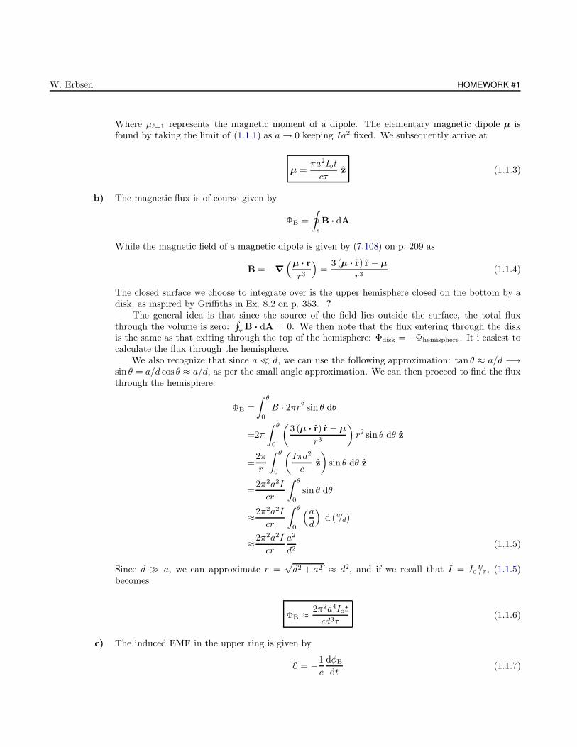
Where µ`=1 represents the magnetic moment of a dipole. The elementary magnetic dipole µ isfound by taking the limit of (1.1.1) as a → 0 keeping Ia2 fixed. We subsequently arrive at
µ =πa2Iot
cτz (1.1.3)
b) The magnetic flux is of course given by
ΦB =
∮
s
B · dA
While the magnetic field of a magnetic dipole is given by (7.108) on p. 209 as
B = −∇
(µ · r
r3
)=
3 (µ · r) r − µ
r3(1.1.4)
The closed surface we choose to integrate over is the upper hemisphere closed on the bottom by adisk, as inspired by Griffiths in Ex. 8.2 on p. 353. ?
The general idea is that since the source of the field lies outside the surface, the total fluxthrough the volume is zero:
∮v B · dA = 0. We then note that the flux entering through the disk
is the same as that exiting through the top of the hemisphere: Φdisk = −Φhemisphere. It i easiest tocalculate the flux through the hemisphere.
We also recognize that since a d, we can use the following approximation: tan θ ≈ a/d −→sin θ = a/d cos θ ≈ a/d, as per the small angle approximation. We can then proceed to find the fluxthrough the hemisphere:
ΦB =
∫ θ
0
B · 2πr2 sin θ dθ
=2π
∫ θ
0
(3 (µ · r) r − µ
r3
)r2 sin θ dθ z
=2π
r
∫ θ
0
(Iπa2
cz
)sin θ dθ z
=2π2a2I
cr
∫ θ
0
sin θ dθ
≈2π2a2I
cr
∫ θ
0
(ad
)d (a/d)
≈2π2a2I
cr
a2
d2(1.1.5)
Since d a, we can approximate r =√d2 + a2 ≈ d2, and if we recall that I = Io
t/τ , (1.1.5)becomes
ΦB ≈ 2π2a4Iot
cd3τ(1.1.6)
c) The induced EMF in the upper ring is given by
E = −1
c
dφB
dt(1.1.7)
CHAPTER 1: ELECTRODYNAMICS II 3
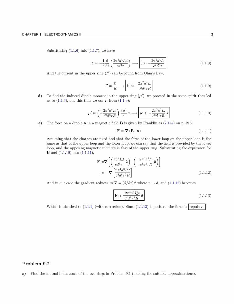
Substituting (1.1.6) into (1.1.7), we have
E ≈ −1
c
d
dt
(2π2a4Iot
cd3τ
)−→ E ≈ −2π2a4Io
c2d3τ(1.1.8)
And the current in the upper ring (I′) can be found from Ohm’s Law,
I′ ≈ E
R−→ I′ ≈ −2π2a4Io
c2d3τR(1.1.9)
d) To find the induced dipole moment in the upper ring (µ′), we proceed in the same spirit that ledus to (1.1.3), but this time we use I′ from (1.1.9):
µ′ ≈(−2π2a4Ioc2d3τR
)πa2
cz −→ µ′ ≈ −2π3a6Io
c3d3τRz (1.1.10)
e) The force on a dipole µ in a magnetic field B is given by Franklin as (7.144) on p. 216:
F = ∇ (B · µ) (1.1.11)
Assuming that the charges are fixed and that the force of the lower loop on the upper loop is thesame as that of the upper loop and the lower loop, we can say that the field is provided by the lowerloop, and the opposing magnetic moment is that of the upper ring. Substituting the expression forB and (1.1.10) into (1.1.11),
F ≈∇
[(πa2Iot
cd3τz
)·(−2π3a6Ioc3d3τR
z
)]
≈− ∇
[2π4a8I2
o t
c4d6τ2R
](1.1.12)
And in our case the gradient reduces to ∇ = (∂/∂r) r where r → d, and (1.1.12) becomes
F ≈ 12π4a8I2o t
c4d7τ2Rz (1.1.13)
Which is identical to (1.1.1) (with correction). Since (1.1.13) is positive, the force is repulsive .
Problem 9.2
a) Find the mutual inductance of the two rings in Problem 9.1 (making the suitable approximations).
W. Erbsen HOMEWORK #1
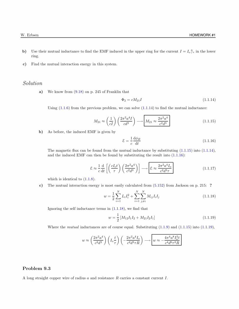
b) Use their mutual inductance to find the EMF induced in the upper ring for the current I = Iot/τ in the lower
ring.
c) Find the mutual interaction energy in this system.
Solution
a) We know from (9.18) on p. 245 of Franklin that
Φ2 = cM21I (1.1.14)
Using (1.1.6) from the previous problem, we can solve (1.1.14) to find the mutual inductance:
M21 ≈(
1
cI
)(2π2a4I
cd3
)−→ M21 ≈ 2π2a4
c2d3(1.1.15)
b) As before, the induced EMF is given by
E =1
c
dφB
dt(1.1.16)
The magnetic flux can be found from the mutual inductance by substituting (1.1.15) into (1.1.14),and the induced EMF can then be found by substituting the result into (1.1.16):
E ≈ 1
c
d
dt
[(cIot
τ
)(2π2a4
c2d3
)]−→ E ≈ 2π2a4Io
c2d3τ(1.1.17)
which is identical to (1.1.8).
c) The mutual interaction energy is most easily calculated from (5.152) from Jackson on p. 215: ?
w =1
2
N∑
i=1
LiI2i +
N∑
i=1
N∑
j 6=i
MijIiIj (1.1.18)
Ignoring the self inductance terms in (1.1.18), we find that
w =1
2[M12I1I2 +M21I2I1] (1.1.19)
Where the mutual inductances are of course equal. Substituting (1.1.9) and (1.1.15) into (1.1.19),
w ≈(
2π2a4
c2d3
)(Iot
τ
)(−2π2a4Ioc2d3τR
)−→ w ≈ −4π4a8I2
o t
c4d6τ2R
Problem 9.3
A long straight copper wire of radius a and resistance R carries a constant current I.
CHAPTER 1: ELECTRODYNAMICS II 5
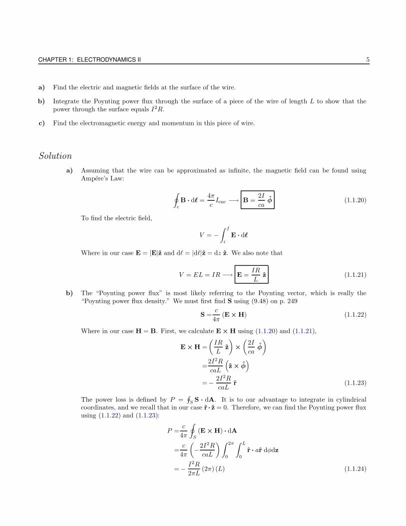
a) Find the electric and magnetic fields at the surface of the wire.
b) Integrate the Poynting power flux through the surface of a piece of the wire of length L to show that thepower through the surface equals I2R.
c) Find the electromagnetic energy and momentum in this piece of wire.
Solution
a) Assuming that the wire can be approximated as infinite, the magnetic field can be found usingAmpere’s Law:
∮
c
B · d` =4π
cIenc −→ B =
2I
caφ (1.1.20)
To find the electric field,
V = −∫ f
i
E · d`
Where in our case E = |E|z and d` = |d`|z = dz z. We also note that
V = EL = IR −→ E =IR
Lz (1.1.21)
b) The “Poynting power flux” is most likely referring to the Poynting vector, which is really the“Poynting power flux density.” We must first find S using (9.48) on p. 249
S =c
4π(E × H) (1.1.22)
Where in our case H = B. First, we calculate E × H using (1.1.20) and (1.1.21),
E × H =
(IR
Lz
)×
(2I
caφ
)
=2I2R
caL
(z × φ
)
= − 2I2R
caLr (1.1.23)
The power loss is defined by P =∮
S S · dA. It is to our advantage to integrate in cylindricalcoordinates, and we recall that in our case r · z = 0. Therefore, we can find the Poynting power fluxusing (1.1.22) and (1.1.23):
P =c
4π
∮
S
(E × H) · dA
=c
4π
(−2I2R
caL
)∫ 2π
0
∫ L
0
r · ar dφdz
= − I2R
2πL(2π) (L) (1.1.24)
W. Erbsen HOMEWORK #1
It is easy to see that (1.1.24) reduces to
P = I2R
c) The electromagnetic energy density is given by (9.47) on p. 249 as
UEM =1
8π(E · D + B · H) (1.1.25)
Where in our case D = E and H = B. Therefore, (1.1.25) becomes
UEM =1
8π
(E2 +B2
)(1.1.26)
Where E and B are the values within the conductor. If we assume that the electric field is uniform,then we can use our previous value. To find the magnetic field,
∮
C
B · d` =4π
c
(πr2)I
πa2−→ B =
2I
ca2r φ (1.1.27)
Substituting (1.1.21) and (1.1.27) into (1.1.26),
UEM =1
8π
[(IR
L
)2
+
(2I
ca2r
)2]
(1.1.28)
To find the electromagnetic energy, we integrate the electromagnetic energy density (1.1.28) overthe entire volume:
w =
∫
V
UEM dτ
=1
8π
∫
V
[(IR
L
)2
+
(2I
ca2r
)2]
dτ
=1
8π
[I2R2
L2
∫r drdφdz +
4I2
c2a4
∫r3 drdφdz
]
=1
8π
[I2R2
L2
∫ a
0
r dr
∫ 2π
0
dφ
∫ L
0
dz +4I2
c2a4
∫ a
0
r3 dr
∫ 2π
0
dφ
∫ L
0
dz
]
=1
8π
[I2R2
L2
(a2
2
)(2π) (L) +
4I2
c2a4
(a4
4
)(2π) (L)
]
Simplifying this expression leads to:
w =I2R2a2
8L+I2L
4c2
The electromagnetic momentum stored in the field is given by (9.80) on p. 255 in Franklin:
PEM =1
4πc
∫
V
E × B dτ (1.1.29)
First calculating the cross product,
E × B =
(IR
Lz
)×
(2I
ca2r φ
)= −2I2R
ca2Lr r (1.1.30)
CHAPTER 1: ELECTRODYNAMICS II 7
Substituting (1.1.30) into (1.1.29),
PEM =1
4πc
∫
V
(−2I2R
ca2Lr
)dτ = − I2R
2πc2a2L
∫ L
0
∫ 2π
0
∫ a
0
r drdφdz −→ PEM = 0
Problem 9.4
The upper and lower curves of the hysteresis loop of a hard ferromagnetic are given by
B+ =Bo [tanh (H/Ho + .5) − .1] , (1.1.31a)
B− =Bo [tanh (H/Ho − .5) + .1] , (1.1.31b)
respectively, for −1.5 < H/Ho < +1.5.
a) Find the energy lost from the magnetic field in one cycle.
b) If Bo = 3 kilogauss, Ho = 1 gauss, and the frequency is 60 Hz, find the power loss in watts.
Solution
a) The work done per unit volume in each cycle of a hysteresis loop is given by the total area,
w =
∮B · dH (1.1.32)
Where B = (B+ − B−). Applying this to (1.1.32) over the specified intervals,
w =
∫ +1.5
−1.5
(B+ − B−) dH
=
∫ +1.5
−1.5
[Bo
(tanh
(H
Ho+ .5
)− .1
)−Bo
(tanh
(H
Ho− .5
)+ .1
)]dH (1.1.33)
If we define α = H/Ho and dα = (1/Ho) dH , (1.1.33) becomes
w =Ho
∫ +1.5
−1.5
[Bo (tanh (α+ .5) − .1) − Bo (tanh (α− .5) + .1)] dα
=BoHo
∫ +1.5
−1.5
tanh (α+ .5) dα−∫ +1.5
−1.5
tanh (α− .5) dα− .2
∫ +1.5
−1.5
dα
=BoHo
[ln [cosh (α+ .5)]
∣∣∣∣+1.5
−1.5
−[
ln [cosh (α− .5)]
∣∣∣∣+1.5
−1.5
− .2
[α
∣∣∣∣+1.5
−1.5
dα
=BoHo ln [cosh (2)]− ln [cosh (1)]− ln [cosh (1)] + ln [cosh (2)] − .6 (1.1.34)
Evaluating (1.1.34) numerically leads to
w ≈ 1.18244 BoHo
W. Erbsen HOMEWORK #1
b) To find the energy loss according to the given parameters,
w ≈ (1.18244)(1 gauss)(3 · 103 gauss)
1/60 Hz−→ w ≈ 212.832 · 103 erg · s−1 (CGS)
w ≈ 212.832 · 10−4 Watts (SI)
Problem 9.5
Two point charges, each of charge q, are a distance 2d apart.
a) Find the Maxwell stress tensor [T] on the plane surface midway between the charges.
b) Find the force on either charge by integrating [T] · dS over a plane surface, closing the surface with a largehemisphere of radius R. (Show that the integral over the hemisphere vanishes in the limit R→ ∞.)
c) Repeat parts (a) and (b) if the charges have opposite signs.
d) What would the force on either charge be if they were immersed in a simple dielectric of infinite extent?
Solution
a) The Maxwell stress tensor is given in Griffiths as (8.19) on p. 352 as
[T] = εo
(EiEj −
1
2δijE
2
)+
1
µo
(BiBj −
1
2δijB
2
)(1.1.35)
For the case in question, our charges are stationary so that the second portion of (1.1.35) vanishes.We can then express [T] in matrix form as
[T] =
Txx Txy Txz
Tyx Tyy Tyz
Tzx Tzy Tzz
= εo
E2
x − 1/2E2 ExEy ExEz
ExEy E2y − 1/2E
2 EyEz
EzEx EyEz E2z − 1/2E
2
In order to resolve the individual components of [T], we must find the corresponding electric fields.We note that the charges are located on the x-axis, and the plane between the charges is theyz-plane. Furthermore, we recall that the electric field of an electric dipole is given by
E =1
4πεo
p
r3(1.1.36)
And in our case r =(x2 + y2 + z2
)1/2 ⇒(d2 + y2 + z2
)1/2. With this in mind, we can now find the
electric fields in the x, y, and z directions respectively:
Ex =0
Ey =1
2πεo
ey
(d2 + y2 + z2)3/2
y ⇒ 1
2πεo
er cos θ
(d2 + r2)3/2
r
Ez =1
2πεo
ez
(d2 + y2 + z2)3/2
z ⇒ 1
2πεo
er sin θ
(d2 + r2)3/2
r
CHAPTER 1: ELECTRODYNAMICS II 9
Where I shamelessly switched to polar coordinates. The total electric field is then
E2 =E2x + E2
y + E2z
=
(1
2πεo
er cos θ
(d2 + r2)3/2
r
)2
+
(1
2πεo
er sin θ
(d2 + r2)3/2
r
)2
=
(e
2πεo
)2r2
(d2 + r2)3
(cos2 θ + sin2 θ
)
=e2
4π2ε2o
r2
(d2 + r2)3
We now have all the tools required to calculate the components of [T]:
Txx = − e2
8π2ε2o
r2
(d2 + r2)3
Tyy =e2
4π2ε2o
r2
(d2 + r2)3
(cos2 θ − 1
2
)
Tyz =Tzy =e2
4π2ε2o
r2
(d2 + r2)3 sin θ cos θ
Tzz =e2
4π2ε2o
r2
(d2 + r2)3
(sin2 θ − 1
2
)
Txy =Txz = Tyx = Tzx = 0
We now define
β =e2
4π2ε2o
r2
(d2 + r2)3(SI)
=4e2r2
(d2 + r2)3 (CGS)
And the Maxwell stress tensor becomes
[T] = εo
−β/2 0 0
0 β(cos2 θ − 1/2
)β sin θ cos θ
0 β sin θ cos θ β(sin2 θ − 1/2
)
b) To integrate the Maxwell stress tensor, we take the route suggested in the prompt. We take ahemisphere of radius R with the base coinciding with the plane surface halfway between the charges(the yz-plane). If we let the hemisphere expand to very large values, then the field at the boundaryof the hemisphere is seen as a dipole, ∝ R−3, and the surface integral then varies like R−4. If wetake R out to infinity, then this portion of the surface integral vanishes since the components of [T]go to zero. There remains then only the force across the plane boundary in the yz-plane.
To find the force on either charge, we integrate [T] · dS over the interstitial plane. We notethat the force is in the x-direction, and the transversal forces are cancelled. Therefore, the onlycomponent of [T] that we need to integrate is Txx, as tabulated previously. We also recall that forthe equatorial disk dS = −r drdφ x, and so the force is
F =
∫
S
[T] dS
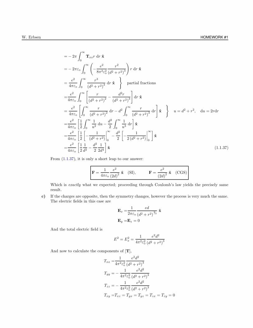
W. Erbsen HOMEWORK #1
= − 2π
∫ ∞
0
Txxr dr x
= − 2πεo
∫ ∞
0
(− e2
8π2ε2o
r2
(d2 + r2)3
)r dr x
=e2
4πεo
∫ ∞
0
r3
(d2 + r2)3 dr x
partial fractions
=e2
4πεo
∫ ∞
0
[r
(d2 + r2)2 − d2r
(d2 + r2)3
]dr x
=e2
4πεo
[∫ ∞
0
r
(d2 + r2)2 dr − d2
∫ ∞
0
r
(d2 + r2)3 dr
]x
u = d2 + r2, du = 2rdr
=e2
4πεo
[1
2
∫ ∞
0
1
u2du− d2
2
∫ ∞
0
1
u3dr
]x
=e2
4πεo
[1
2
[− 1
(d2 + r2)
∣∣∣∣∞
0
− d2
2
[− 1
2 (d2 + r2)
∣∣∣∣∞
0
]x
=e2
4πεo
[1
2
1
d2− d2
2
1
2d4
]x (1.1.37)
From (1.1.37), it is only a short leap to our answer:
F =1
4πεo
e2
(2d)2 x (SI), F =
e2
(2d)2 x (CGS)
Which is exactly what we expected; proceeding through Coulomb’s law yields the precisely sameresult.
c) If the charges are opposite, then the symmetry changes, however the process is very much the same.The electric fields in this case are
Ex =1
2πεo
ed
(d2 + r2)3/2
x
Ey =Ez = 0
And the total electric field is
E2 = E2x =
1
4π2ε2o
e2d2
(d2 + r2)3
And now to calculate the components of [T],
Txx =1
4π2ε2o
e2d2
(d2 + r2)3
Tyy = − 1
4π2ε2o
e2d2
(d2 + r2)3
Tzz = − 1
4π2ε2o
e2d2
(d2 + r2)3
Txy =Txz = Tyx = Tyz = Tzx = Tzy = 0
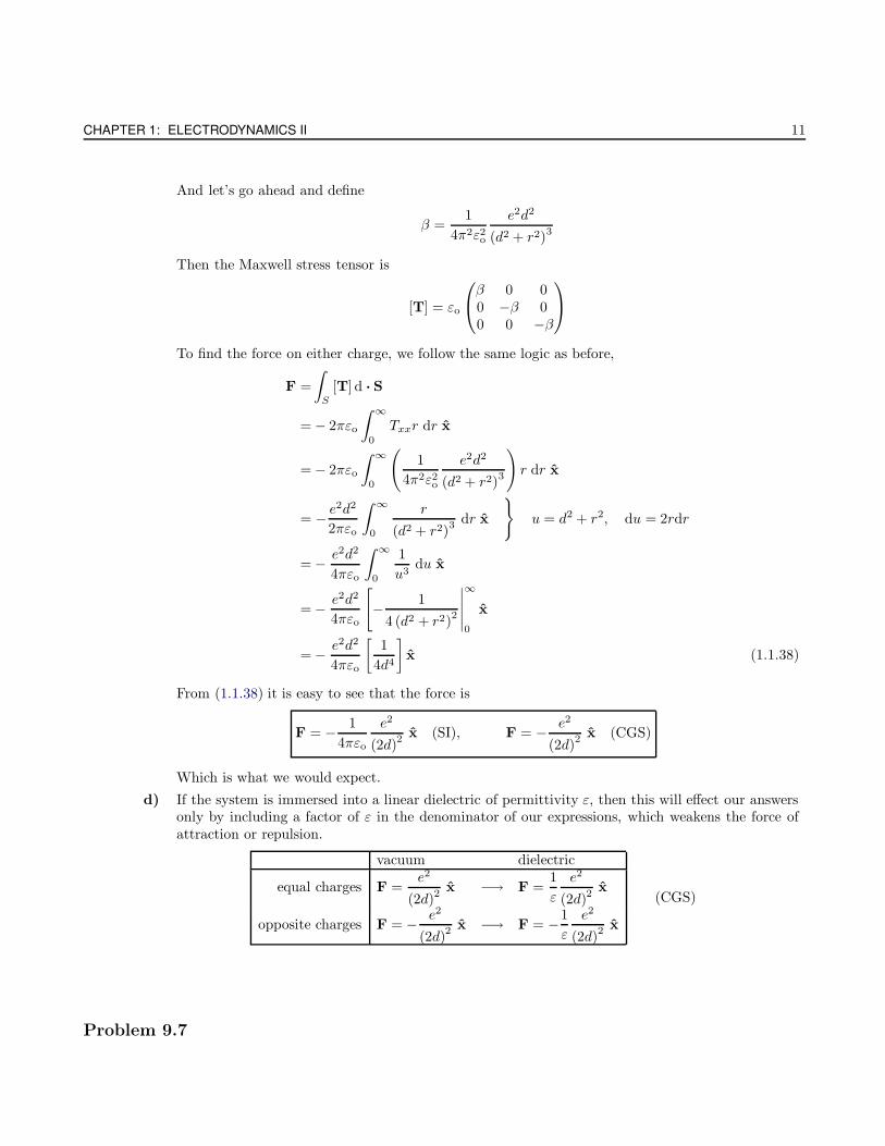
CHAPTER 1: ELECTRODYNAMICS II 11
And let’s go ahead and define
β =1
4π2ε2o
e2d2
(d2 + r2)3
Then the Maxwell stress tensor is
[T] = εo
β 0 00 −β 00 0 −β
To find the force on either charge, we follow the same logic as before,
F =
∫
S
[T] d · S
= − 2πεo
∫ ∞
0
Txxr dr x
= − 2πεo
∫ ∞
0
(1
4π2ε2o
e2d2
(d2 + r2)3
)r dr x
= − e2d2
2πεo
∫ ∞
0
r
(d2 + r2)3 dr x
u = d2 + r2, du = 2rdr
= − e2d2
4πεo
∫ ∞
0
1
u3du x
= − e2d2
4πεo
[− 1
4 (d2 + r2)2
∣∣∣∣∣
∞
0
x
= − e2d2
4πεo
[1
4d4
]x (1.1.38)
From (1.1.38) it is easy to see that the force is
F = − 1
4πεo
e2
(2d)2 x (SI), F = − e2
(2d)2 x (CGS)
Which is what we would expect.
d) If the system is immersed into a linear dielectric of permittivity ε, then this will effect our answersonly by including a factor of ε in the denominator of our expressions, which weakens the force ofattraction or repulsion.
vacuum dielectric
equal charges F =e2
(2d)2x −→ F =
1
ε
e2
(2d)2x
opposite charges F = − e2
(2d)2 x −→ F = −1
ε
e2
(2d)2 x
(CGS)
Problem 9.7
W. Erbsen HOMEWORK #1
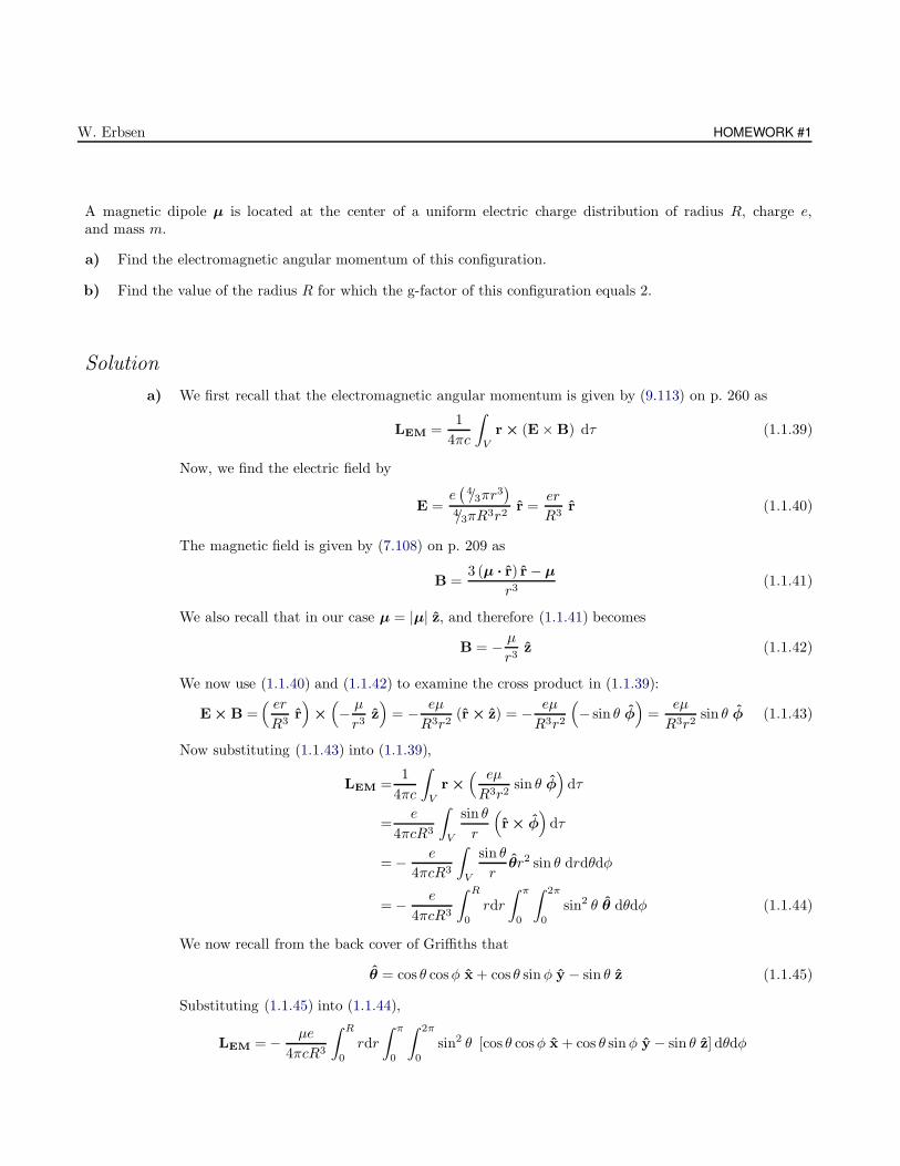
A magnetic dipole µ is located at the center of a uniform electric charge distribution of radius R, charge e,and mass m.
a) Find the electromagnetic angular momentum of this configuration.
b) Find the value of the radius R for which the g-factor of this configuration equals 2.
Solution
a) We first recall that the electromagnetic angular momentum is given by (9.113) on p. 260 as
LEM =1
4πc
∫
V
r × (E × B) dτ (1.1.39)
Now, we find the electric field by
E =e(
4/3πr3)
4/3πR3r2r =
er
R3r (1.1.40)
The magnetic field is given by (7.108) on p. 209 as
B =3 (µ · r) r − µ
r3(1.1.41)
We also recall that in our case µ = |µ| z, and therefore (1.1.41) becomes
B = − µ
r3z (1.1.42)
We now use (1.1.40) and (1.1.42) to examine the cross product in (1.1.39):
E × B =( erR3
r)
×
(− µ
r3z)
= − eµ
R3r2(r × z) = − eµ
R3r2
(− sin θ φ
)=
eµ
R3r2sin θ φ (1.1.43)
Now substituting (1.1.43) into (1.1.39),
LEM =1
4πc
∫
V
r ×
( eµ
R3r2sin θ φ
)dτ
=e
4πcR3
∫
V
sin θ
r
(r × φ
)dτ
= − e
4πcR3
∫
V
sin θ
rθr2 sin θ drdθdφ
= − e
4πcR3
∫ R
0
rdr
∫ π
0
∫ 2π
0
sin2 θ θ dθdφ (1.1.44)
We now recall from the back cover of Griffiths that
θ = cos θ cosφ x + cos θ sinφ y − sin θ z (1.1.45)
Substituting (1.1.45) into (1.1.44),
LEM = − µe
4πcR3
∫ R
0
rdr
∫ π
0
∫ 2π
0
sin2 θ [cos θ cosφ x + cos θ sinφ y − sin θ z] dθdφ
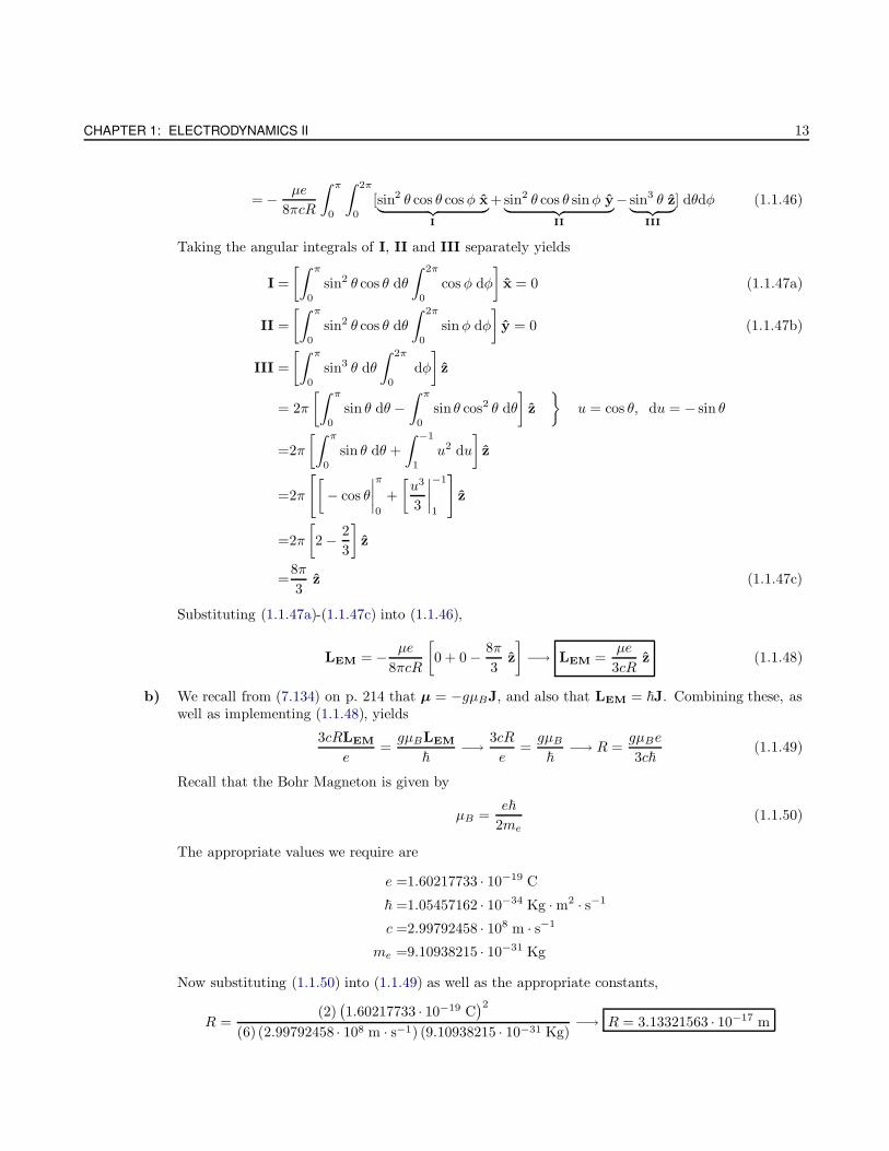
CHAPTER 1: ELECTRODYNAMICS II 13
= − µe
8πcR
∫ π
0
∫ 2π
0
[sin2 θ cos θ cos φ x︸ ︷︷ ︸I
+sin2 θ cos θ sinφ y︸ ︷︷ ︸II
− sin3 θ z︸ ︷︷ ︸III
] dθdφ (1.1.46)
Taking the angular integrals of I, II and III separately yields
I =
[∫ π
0
sin2 θ cos θ dθ
∫ 2π
0
cos φ dφ
]x = 0 (1.1.47a)
II =
[∫ π
0
sin2 θ cos θ dθ
∫ 2π
0
sinφ dφ
]y = 0 (1.1.47b)
III =
[∫ π
0
sin3 θ dθ
∫ 2π
0
dφ
]z
= 2π
[∫ π
0
sin θ dθ −∫ π
0
sin θ cos2 θ dθ
]z
u = cos θ, du = − sin θ
=2π
[∫ π
0
sin θ dθ +
∫ −1
1
u2 du
]z
=2π
[[− cos θ
∣∣∣∣π
0
+
[u3
3
∣∣∣∣−1
1
]z
=2π
[2 − 2
3
]z
=8π
3z (1.1.47c)
Substituting (1.1.47a)-(1.1.47c) into (1.1.46),
LEM = − µe
8πcR
[0 + 0 − 8π
3z
]−→ LEM =
µe
3cRz (1.1.48)
b) We recall from (7.134) on p. 214 that µ = −gµBJ, and also that LEM = ~J. Combining these, aswell as implementing (1.1.48), yields
3cRLEM
e=gµBLEM
~−→ 3cR
e=gµB
~−→ R =
gµBe
3c~(1.1.49)
Recall that the Bohr Magneton is given by
µB =e~
2me(1.1.50)
The appropriate values we require are
e =1.60217733 · 10−19 C
~ =1.05457162 · 10−34 Kg · m2 · s−1
c =2.99792458 · 108 m · s−1
me =9.10938215 · 10−31 Kg
Now substituting (1.1.50) into (1.1.49) as well as the appropriate constants,
R =(2)(1.60217733 · 10−19 C
)2
(6) (2.99792458 · 108 m · s−1) (9.10938215 · 10−31 Kg)−→ R = 3.13321563 · 10−17 m
W. Erbsen HOMEWORK #2
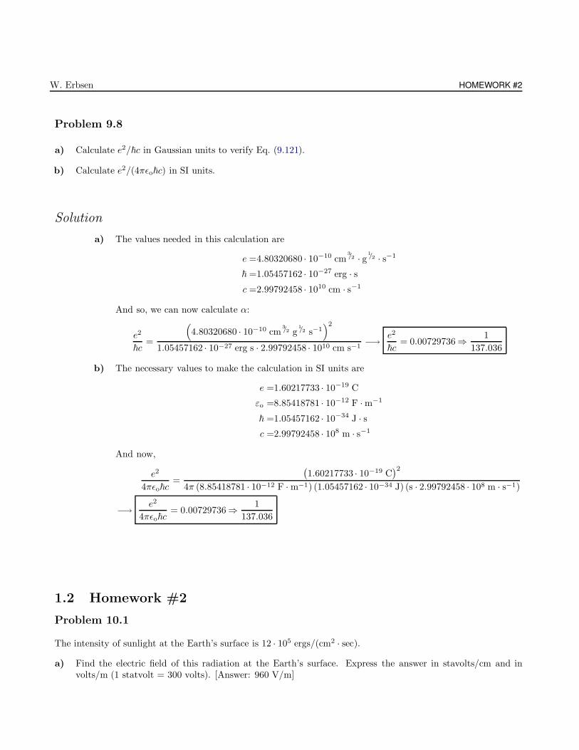
Problem 9.8
a) Calculate e2/~c in Gaussian units to verify Eq. (9.121).
b) Calculate e2/(4πεo~c) in SI units.
Solution
a) The values needed in this calculation are
e =4.80320680 · 10−10 cm3/2 · g 1/2 · s−1
~ =1.05457162 · 10−27 erg · sc =2.99792458 · 1010 cm · s−1
And so, we can now calculate α:
e2
~c=
(4.80320680 · 10−10 cm
3/2 g1/2 s−1
)2
1.05457162 · 10−27 erg s · 2.99792458 · 1010 cm s−1−→ e2
~c= 0.00729736 ⇒ 1
137.036
b) The necessary values to make the calculation in SI units are
e =1.60217733 · 10−19 C
εo =8.85418781 · 10−12 F ·m−1
~ =1.05457162 · 10−34 J · sc =2.99792458 · 108 m · s−1
And now,
e2
4πεo~c=
(1.60217733 · 10−19 C
)2
4π (8.85418781 · 10−12 F · m−1) (1.05457162 · 10−34 J) (s · 2.99792458 · 108 m · s−1)
−→ e2
4πεo~c= 0.00729736 ⇒ 1
137.036
1.2 Homework #2
Problem 10.1
The intensity of sunlight at the Earth’s surface is 12 · 105 ergs/(cm2 · sec).
a) Find the electric field of this radiation at the Earth’s surface. Express the answer in stavolts/cm and involts/m (1 statvolt = 300 volts). [Answer: 960 V/m]
CHAPTER 1: ELECTRODYNAMICS II 15
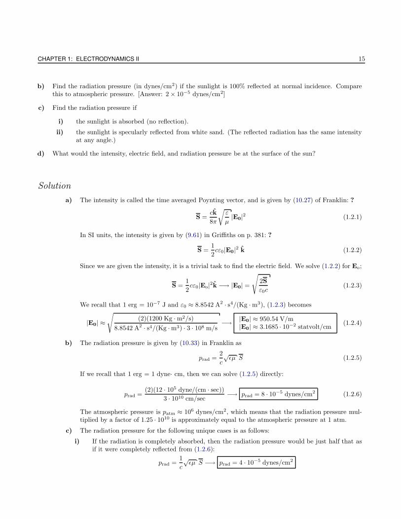
b) Find the radiation pressure (in dynes/cm2) if the sunlight is 100% reflected at normal incidence. Comparethis to atmospheric pressure. [Answer: 2 × 10⁻⁵ dynes/cm2]
c) Find the radiation pressure if
i) the sunlight is absorbed (no reflection).
ii) the sunlight is specularly reflected from white sand. (The reflected radiation has the same intensityat any angle.)
d) What would the intensity, electric field, and radiation pressure be at the surface of the sun?
Solution
a) The intensity is called the time averaged Poynting vector, and is given by (10.27) of Franklin: ?
S =ck
8π
√ε
µ|E0|2 (1.2.1)
In SI units, the intensity is given by (9.61) in Griffiths on p. 381: ?
S =1
2cε0|E0|2 k (1.2.2)
Since we are given the intensity, it is a trivial task to find the electric field. We solve (1.2.2) for Eo;
S =1
2cε0|Eo|2k −→ |E0| =
√2S
ε0c(1.2.3)
We recall that 1 erg = 10−7 J and ε0 ≈ 8.8542 A2 · s4/(Kg ·m3), (1.2.3) becomes
|E0| ≈√
(2)(1200 Kg · m2/s)
8.8542 A2 · s4/(Kg ·m3) · 3 · 108 m/s−→ |E0| ≈ 950.54 V/m
|E0| ≈ 3.1685 · 10−2 statvolt/cm(1.2.4)
b) The radiation pressure is given by (10.33) in Franklin as
prad =2
c
√εµ S (1.2.5)
If we recall that 1 erg = 1 dyne· cm, then we can solve (1.2.5) directly:
prad =(2)(12 · 105 dyne/(cm · sec))
3 · 1010 cm/sec−→ prad = 8 · 10−5 dynes/cm2 (1.2.6)
The atmospheric pressure is patm ≈ 106 dynes/cm2, which means that the radiation pressure mul-tiplied by a factor of 1.25 · 1010 is approximately equal to the atmospheric pressure at 1 atm.
c) The radiation pressure for the following unique cases is as follows:
i) If the radiation is completely absorbed, then the radiation pressure would be just half that asif it were completely reflected from (1.2.6):
prad =1
c
√εµ S −→ prad = 4 · 10−5 dynes/cm2
W. Erbsen HOMEWORK #2
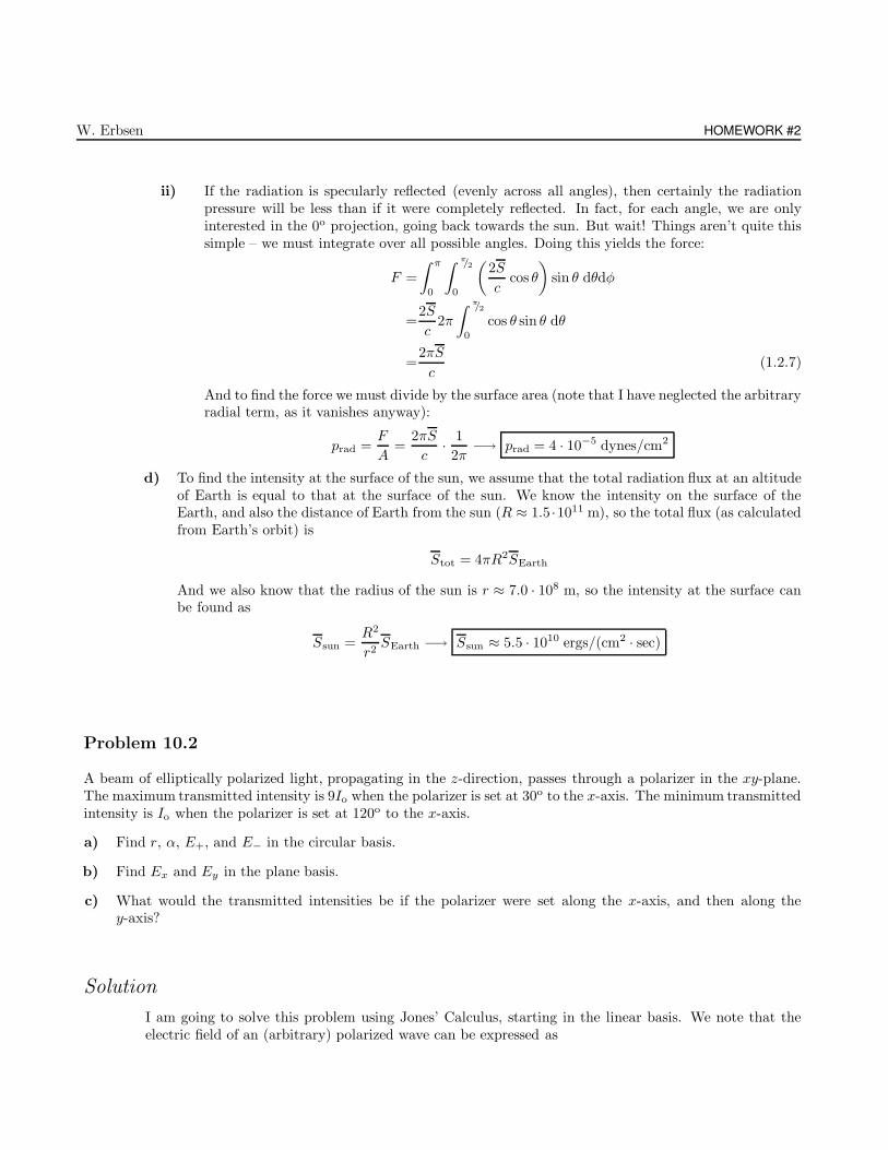
ii) If the radiation is specularly reflected (evenly across all angles), then certainly the radiationpressure will be less than if it were completely reflected. In fact, for each angle, we are onlyinterested in the 0o projection, going back towards the sun. But wait! Things aren’t quite thissimple – we must integrate over all possible angles. Doing this yields the force:
F =
∫ π
0
∫ π/2
0
(2S
ccos θ
)sin θ dθdφ
=2S
c2π
∫ π/2
0
cos θ sin θ dθ
=2πS
c(1.2.7)
And to find the force we must divide by the surface area (note that I have neglected the arbitraryradial term, as it vanishes anyway):
prad =F
A=
2πS
c· 1
2π−→ prad = 4 · 10−5 dynes/cm2
d) To find the intensity at the surface of the sun, we assume that the total radiation flux at an altitudeof Earth is equal to that at the surface of the sun. We know the intensity on the surface of theEarth, and also the distance of Earth from the sun (R ≈ 1.5 ·1011 m), so the total flux (as calculatedfrom Earth’s orbit) is
Stot = 4πR2SEarth
And we also know that the radius of the sun is r ≈ 7.0 · 108 m, so the intensity at the surface canbe found as
Ssun =R2
r2SEarth −→ Ssun ≈ 5.5 · 1010 ergs/(cm2 · sec)
Problem 10.2
A beam of elliptically polarized light, propagating in the z-direction, passes through a polarizer in the xy-plane.The maximum transmitted intensity is 9Io when the polarizer is set at 30o to the x-axis. The minimum transmittedintensity is Io when the polarizer is set at 120o to the x-axis.
a) Find r, α, E+, and E− in the circular basis.
b) Find Ex and Ey in the plane basis.
c) What would the transmitted intensities be if the polarizer were set along the x-axis, and then along they-axis?
Solution
I am going to solve this problem using Jones’ Calculus, starting in the linear basis. We note that theelectric field of an (arbitrary) polarized wave can be expressed as
CHAPTER 1: ELECTRODYNAMICS II 17
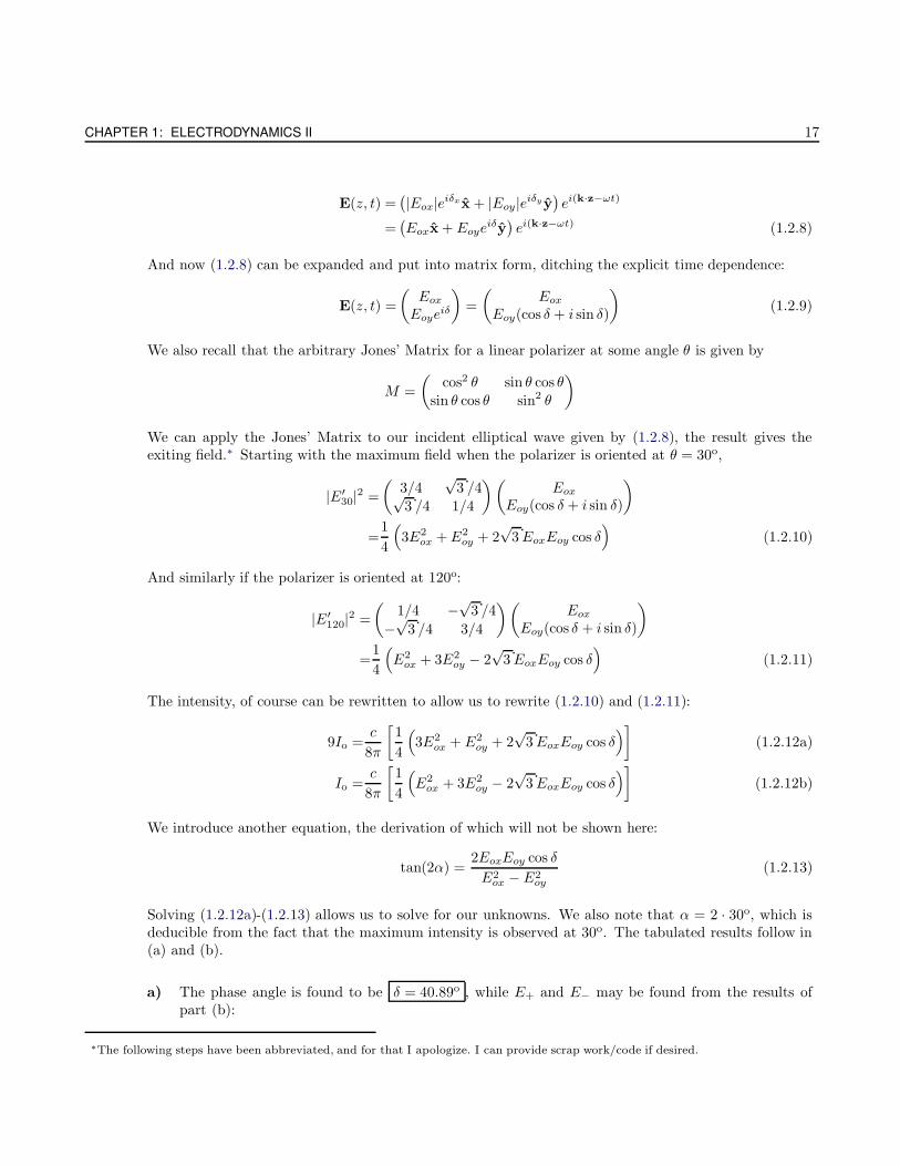
E(z, t) =(|Eox|eiδxx + |Eoy|eiδy y
)ei(k·z−ωt)
=(Eoxx + Eoye
iδy)ei(k·z−ωt) (1.2.8)
And now (1.2.8) can be expanded and put into matrix form, ditching the explicit time dependence:
E(z, t) =
(Eox
Eoyeiδ
)=
(Eox
Eoy(cos δ + i sin δ)
)(1.2.9)
We also recall that the arbitrary Jones’ Matrix for a linear polarizer at some angle θ is given by
M =
(cos2 θ sin θ cos θ
sin θ cos θ sin2 θ
)
We can apply the Jones’ Matrix to our incident elliptical wave given by (1.2.8), the result gives theexiting field.∗ Starting with the maximum field when the polarizer is oriented at θ = 30o,
|E′30|2 =
(3/4
√3 /4√
3 /4 1/4
)(Eox
Eoy(cos δ + i sin δ)
)
=1
4
(3E2
ox +E2oy + 2
√3EoxEoy cos δ
)(1.2.10)
And similarly if the polarizer is oriented at 120o:
|E′120|2 =
(1/4 −
√3 /4
−√
3 /4 3/4
)(Eox
Eoy(cos δ + i sin δ)
)
=1
4
(E2
ox + 3E2oy − 2
√3EoxEoy cos δ
)(1.2.11)
The intensity, of course can be rewritten to allow us to rewrite (1.2.10) and (1.2.11):
9Io =c
8π
[1
4
(3E2
ox + E2oy + 2
√3EoxEoy cos δ
)](1.2.12a)
Io =c
8π
[1
4
(E2
ox + 3E2oy − 2
√3EoxEoy cos δ
)](1.2.12b)
We introduce another equation, the derivation of which will not be shown here:
tan(2α) =2EoxEoy cos δ
E2ox − E2
oy
(1.2.13)
Solving (1.2.12a)-(1.2.13) allows us to solve for our unknowns. We also note that α = 2 · 30o, which isdeducible from the fact that the maximum intensity is observed at 30o. The tabulated results follow in(a) and (b).
a) The phase angle is found to be δ = 40.89o , while E+ and E− may be found from the results ofpart (b):
∗The following steps have been abbreviated, and for that I apologize. I can provide scrap work/code if desired.
W. Erbsen HOMEWORK #2
E+ = Ex + iEy =
√Ioc
(13.26 cos(ωt) + i8.86 cos (ωt− 40.89o))
E− = Ex − iEy =
√Ioc
(13.26 cos(ωt) − i8.86 cos (ωt − 40.89o))
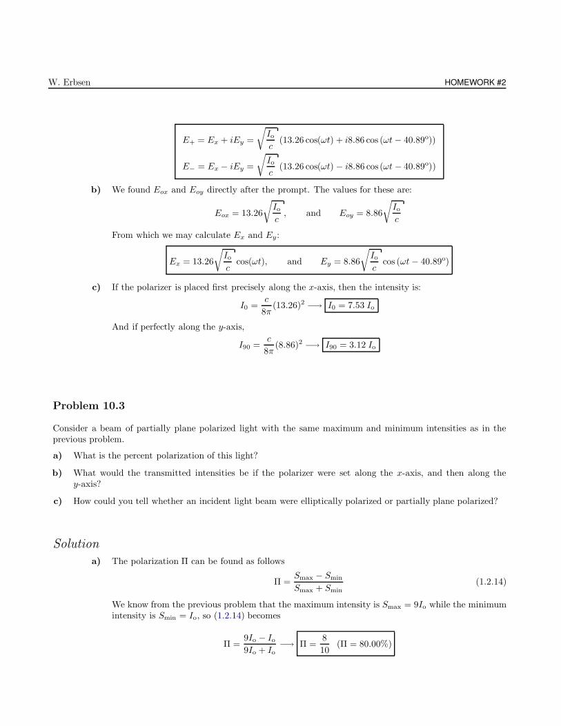
b) We found Eox and Eoy directly after the prompt. The values for these are:
Eox = 13.26
√Ioc, and Eoy = 8.86
√Ioc
From which we may calculate Ex and Ey:
Ex = 13.26
√Ioc
cos(ωt), and Ey = 8.86
√Ioc
cos (ωt− 40.89o)
c) If the polarizer is placed first precisely along the x-axis, then the intensity is:
I0 =c
8π(13.26)2 −→ I0 = 7.53 Io
And if perfectly along the y-axis,
I90 =c
8π(8.86)2 −→ I90 = 3.12 Io
Problem 10.3
Consider a beam of partially plane polarized light with the same maximum and minimum intensities as in theprevious problem.
a) What is the percent polarization of this light?
b) What would the transmitted intensities be if the polarizer were set along the x-axis, and then along they-axis?
c) How could you tell whether an incident light beam were elliptically polarized or partially plane polarized?
Solution
a) The polarization Π can be found as follows
Π =Smax − Smin
Smax + Smin(1.2.14)
We know from the previous problem that the maximum intensity is Smax = 9Io while the minimumintensity is Smin = Io, so (1.2.14) becomes
Π =9Io − Io9Io + Io
−→ Π =8
10(Π = 80.00%)
CHAPTER 1: ELECTRODYNAMICS II 19
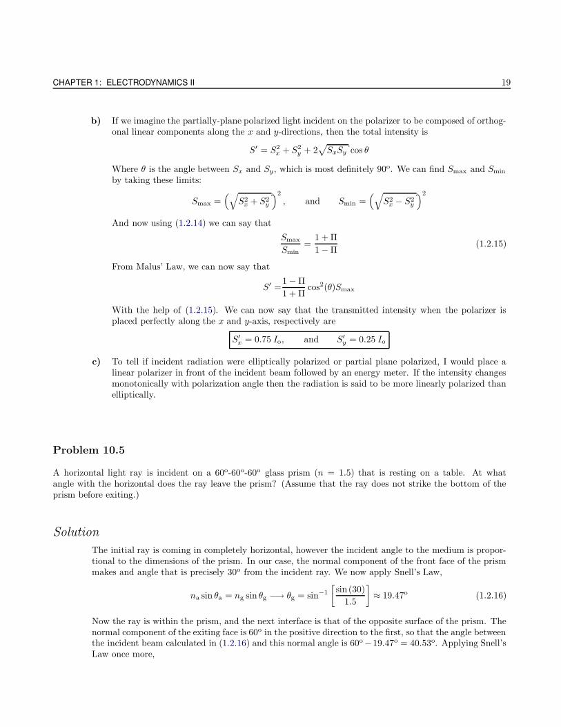
b) If we imagine the partially-plane polarized light incident on the polarizer to be composed of orthog-onal linear components along the x and y-directions, then the total intensity is
S′ = S2x + S2
y + 2√SxSy cos θ
Where θ is the angle between Sx and Sy, which is most definitely 90o. We can find Smax and Smin
by taking these limits:
Smax =(√
S2x + S2
y
)2
, and Smin =(√
S2x − S2
y
)2
And now using (1.2.14) we can say that
Smax
Smin=
1 + Π
1 − Π(1.2.15)
From Malus’ Law, we can now say that
S′ =1 − Π
1 + Πcos2(θ)Smax
With the help of (1.2.15). We can now say that the transmitted intensity when the polarizer isplaced perfectly along the x and y-axis, respectively are
S′x = 0.75 Io, and S′
y = 0.25 Io
c) To tell if incident radiation were elliptically polarized or partial plane polarized, I would place alinear polarizer in front of the incident beam followed by an energy meter. If the intensity changesmonotonically with polarization angle then the radiation is said to be more linearly polarized thanelliptically.
Problem 10.5
A horizontal light ray is incident on a 60o-60o-60o glass prism (n = 1.5) that is resting on a table. At whatangle with the horizontal does the ray leave the prism? (Assume that the ray does not strike the bottom of theprism before exiting.)
Solution
The initial ray is coming in completely horizontal, however the incident angle to the medium is propor-tional to the dimensions of the prism. In our case, the normal component of the front face of the prismmakes and angle that is precisely 30o from the incident ray. We now apply Snell’s Law,
na sin θa = ng sin θg −→ θg = sin−1
[sin (30)
1.5
]≈ 19.47o (1.2.16)
Now the ray is within the prism, and the next interface is that of the opposite surface of the prism. Thenormal component of the exiting face is 60o in the positive direction to the first, so that the angle betweenthe incident beam calculated in (1.2.16) and this normal angle is 60o−19.47o = 40.53o. Applying Snell’sLaw once more,
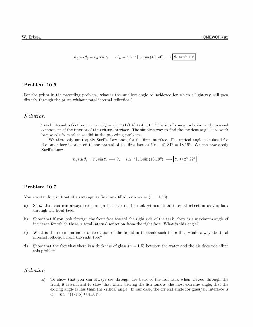
W. Erbsen HOMEWORK #2
ng sin θg = na sin θa −→ θa = sin−1 [1.5 sin (40.53)] −→ θa ≈ 77.10o
Problem 10.6
For the prism in the preceding problem, what is the smallest angle of incidence for which a light ray will passdirectly through the prism without total internal reflection?
Solution
Total internal reflection occurs at θc = sin−1 (1/1.5) ≈ 41.81o. This is, of course, relative to the normalcomponent of the interior of the exiting interface. The simplest way to find the incident angle is to workbackwards from what we did in the preceding problem.
We then only must apply Snell’s Law once, for the first interface. The critical angle calculated forthe outer face is oriented to the normal of the first face as 60o − 41.81o = 18.19o. We can now applySnell’s Law:
ng sin θg = na sin θa −→ θa = sin−1 [1.5 sin(18.19o)] −→ θa ≈ 27.92o
Problem 10.7
You are standing in front of a rectangular fish tank filled with water (n = 1.33).
a) Show that you can always see through the back of the tank without total internal reflection as you lookthrough the front face.
b) Show that if you look through the front face toward the right side of the tank, there is a maximum angle ofincidence for which there is total internal reflection from the right face. What is this angle?
c) What is the minimum index of refraction of the liquid in the tank such there that would always be totalinternal reflection from the right face?
d) Show that the fact that there is a thickness of glass (n = 1.5) between the water and the air does not affectthis problem.
Solution
a) To show that you can always see through the back of the fish tank when viewed through thefront, it is sufficient to show that when viewing the fish tank at the most extreme angle, that theexiting angle is less than the critical angle. In our case, the critical angle for glass/air interface isθc = sin−1 (1/1.5) ≈ 41.81o.
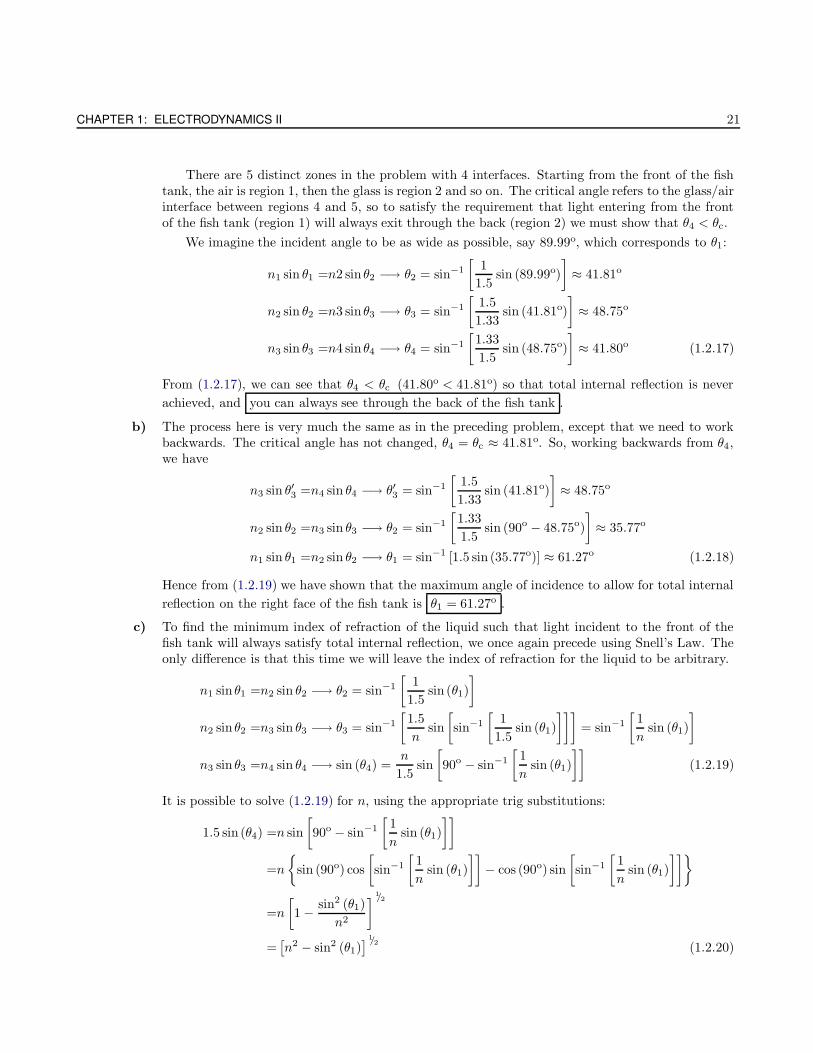
CHAPTER 1: ELECTRODYNAMICS II 21
There are 5 distinct zones in the problem with 4 interfaces. Starting from the front of the fishtank, the air is region 1, then the glass is region 2 and so on. The critical angle refers to the glass/airinterface between regions 4 and 5, so to satisfy the requirement that light entering from the frontof the fish tank (region 1) will always exit through the back (region 2) we must show that θ4 < θc.
We imagine the incident angle to be as wide as possible, say 89.99o, which corresponds to θ1:
n1 sin θ1 =n2 sin θ2 −→ θ2 = sin−1
[1
1.5sin (89.99o)
]≈ 41.81o
n2 sin θ2 =n3 sin θ3 −→ θ3 = sin−1
[1.5
1.33sin (41.81o)
]≈ 48.75o
n3 sin θ3 =n4 sin θ4 −→ θ4 = sin−1
[1.33
1.5sin (48.75o)
]≈ 41.80o (1.2.17)
From (1.2.17), we can see that θ4 < θc (41.80o < 41.81o) so that total internal reflection is never
achieved, and you can always see through the back of the fish tank .
b) The process here is very much the same as in the preceding problem, except that we need to workbackwards. The critical angle has not changed, θ4 = θc ≈ 41.81o. So, working backwards from θ4,we have
n3 sin θ′3 =n4 sin θ4 −→ θ′3 = sin−1
[1.5
1.33sin (41.81o)
]≈ 48.75o
n2 sin θ2 =n3 sin θ3 −→ θ2 = sin−1
[1.33
1.5sin (90o − 48.75o)
]≈ 35.77o
n1 sin θ1 =n2 sin θ2 −→ θ1 = sin−1 [1.5 sin (35.77o)] ≈ 61.27o (1.2.18)
Hence from (1.2.19) we have shown that the maximum angle of incidence to allow for total internal
reflection on the right face of the fish tank is θ1 = 61.27o .
c) To find the minimum index of refraction of the liquid such that light incident to the front of thefish tank will always satisfy total internal reflection, we once again precede using Snell’s Law. Theonly difference is that this time we will leave the index of refraction for the liquid to be arbitrary.
n1 sin θ1 =n2 sin θ2 −→ θ2 = sin−1
[1
1.5sin (θ1)
]
n2 sin θ2 =n3 sin θ3 −→ θ3 = sin−1
[1.5
nsin
[sin−1
[1
1.5sin (θ1)
]]]= sin−1
[1
nsin (θ1)
]
n3 sin θ3 =n4 sin θ4 −→ sin (θ4) =n
1.5sin
[90o − sin−1
[1
nsin (θ1)
]](1.2.19)
It is possible to solve (1.2.19) for n, using the appropriate trig substitutions:
1.5 sin (θ4) =n sin
[90o − sin−1
[1
nsin (θ1)
]]
=n
sin (90o) cos
[sin−1
[1
nsin (θ1)
]]− cos (90o) sin
[sin−1
[1
nsin (θ1)
]]
=n
[1 − sin2 (θ1)
n2
]1/2
=[n2 − sin2 (θ1)
] 1/2(1.2.20)
W. Erbsen HOMEWORK #2
If we recall that θ4 = θc and imagine our incident angle to the most extreme position of θ1 = 89.99o,(1.2.20) can be solved to find the minimum index of refraction:
n =[(1.5)2 sin2 (41.81o) + sin2 (89.99o)
]1/2−→ n ≈ 1.41 (1.2.21)
d) The fact that the width of the glass is negligible can be shown by recomputing the results of parts(a) and (b) with assuming that there is no glass media. For part (a), where we are asked to showthat total internal reflection is never satisfied if viewing through the front of the tank, we start withthe critical angle at the second interface, which is θc = sin−1 (1/1.33) ≈ 48.75o, and applying Snell’sLaw:
n1 sin θ1 = n2 sin θc −→ θ1 =sin−1 [1.33 sin (48.75o)] = 90o
Since you can never see through the fish tank at exactly 90o, we have shown that the criticalcondition cannot be satisfied, as previously shown in (1.2.17).
For part (b), we can similarly work backwards from the critical angle:
n1 sin θ1 = n2 sin θc −→ θ1 =sin−1 [1.33 sin (90o − 48.75o)] ≈ 61.27o (1.2.22)
As can be seen, (1.2.22) matches (1.2.19), and therefore from these two instances we are forced to
admit that the width of the glass is irrelevant .
Problem 10.9
a) Solve Eqs. (10.117)-(10.120), to get the transmitted and reflected electric fields given by Eqs. (10.121) and(10.122).
b) Use these fields to get the transmission and reflection coefficients for the coated surface.
c) For an original air (n = 1) to glass (n = 1.5) interface, find the index of refraction and thickness of a coatingthat would have no reflection at the incident wavelength of 5, 000A.
Solution
a) Equations (10.117)-(10.120) read
E1 +E′1 =E2 +E′
2eik2d (1.2.23a)
n1(E1 − E′1) =n2(E2 − E′
2eik2d) (1.2.23b)
E2eik2d +E′
2 =E3 (1.2.23c)
n2(E2eik2d − E′
2) =n3E3 (1.2.23d)
We start with (1.2.23a) and rearrange it:
E′1 = E2 + E′
2eik2d −E1 (1.2.24)
CHAPTER 1: ELECTRODYNAMICS II 23
We now substitute (1.2.24) into (1.2.23b):
n1
[E1 −
(E2 +E′
2eik2d − E1
)]=n2
[E2 − E′
2eik2d]
n1
[E1 − E2 − E′
2eik2d + E2
]=n2
[E2 − E′
2eik2d]
2n1E1 − n1E2 − n1E′2e
ik2d =n2E2 − E′2n2e
ik2d
n2E′2e
ik2d − n1E′2e
ik2d =n2E2 + n1E2 − 2n1E1
−→ E′2 = e−ik2d
[E2(n2 + n1) − 2n1E1
n2 − n1
](1.2.25)
We now take (1.2.25) and substitute it into (1.2.23c):
E2eik2d + e−ik2d
[E2(n2 + n1) − 2n1E1
n2 − n1
]= E3
E3(n2 − n1) =E2(n2 − n1)eik2d +E2(n2 + n1)e
−ik2d − 2n1E1e−ik2d
2E1n1e−ik2d + E3(n2 − n1) =E2(n2 − n1)e
ik2d +E2(n2 + n1)e−ik2d
=E2
[n2e
ik2d − n1eik2d + n2e
−ik2d + n1e−ik2d
]
=E2
[n2
(eik2d + e−ik2d
)− n1
(eik2d − e−ik2d
)]
=E2 [2n2 cos(k2d) − 2in1 sin(k2d)]
=2E2 [n2 cos(k2d) − in1 sin(k2d)]
−→ E2 =2E1n1e
−ik2d +E3(n2 − n1)
2 [n2 cos(k2d) − in1 sin(k2d)](1.2.26)
We perform a similar exercise by substituting (1.2.25) into (1.2.23d):
n3E3 =n2
[E2e
ik2d − e−ik2d
[E2(n2 + n1) − 2n1E1
n2 − n1
]]
n3E3 =n2E2eik2d − E2(n2 + n1)n2e
−ik2d + 2n1n2E1e−ik2d
n2 − n1
n3(n2 − n1)E3 =n2(n2 − n1)E2eik2d − n2E2(n2 + n1)e
−ik2d + 2n1n2E1e−ik2d
n3(n2 − n1)E3 − 2n1n2E1e−ik2d =n2E2
[n2e
ik2d − n1eik2d − n2e
−ik2d − n1e−ik2d
]
=n2E2
[n2
(eik2d − e−ik2d
)− n1
(eik2d − e−ik2d
)]
=n2E2 [2in2 sin(k2d) − 2n1 cos(k2)d)]
−→ E2 =n3(n2 − n1)E3 − 2n1n2E1e
−ik2d
2n2 [in2 sin(k2d) − n1 cos(k2d)](1.2.27)
We can now set (1.2.26) and (1.2.27) equal to one another to eliminate E2:
2E1n1e−ik2d + E3(n2 − n1)
2 [n2 cos(k2d) − in1 sin(k2d)]=n3(n2 − n1)E3 − 2n1n2E1e
−ik2d
2n2 [in2 sin(k2d) − n1 cos(k2d)](1.2.28)
If we let α = sin k2d and β = cos k2d, then (1.2.28) becomes
2E1n1e−ik2d +E3(n2 − n1)
n2β − in1α=n3(n2 − n1)E3 − 2n1n2E1e
−ik2d
in22α− n1n2β
2E1n1e−ik2d
n2β − in1α+
2n1n2E1e−ik2d
in22α− n1n2β︸ ︷︷ ︸
I
=n3(n2 − n1)E3
in22α− n1n2β
− E3(n2 − n1)
n2β − in1α︸ ︷︷ ︸II
W. Erbsen HOMEWORK #2
Where I have separated our expression for simplicity. The components are:
I =2E1n1e
−ik2d
n2β − in1α· n2β + in1α
n2β + in1α+
2n1n2E1e−ik2d
in22α− n1n2β
· in22α+ n1n2β
in22α+ n1n2β
=2E1n1e
−ik2d (n2β + in1α)
n22β
2 + n21α
2− 2n1n2E1e
−ik2d(in2
2α+ n1n2β)
n21n
22β
2 + n42α
2
=2E1n1(n2 − n1)E1(iα+ β)
(n2α+ in1β)(n1α+ in2β)
=2E1n1(n2 − n1)E1(i sin(k2d) + cos(k2d))
(n2 sin(k2d) + in1 cos(k2d))(n1 sin(k2d) + in2 cos(k2d))
=4in1(n1 − n2)E1
2in1n2 cos(2k2d) + (n21 + n2
2) sin(2kdd)(1.2.29)
And now
II =n3(n2 − n1)E3
in22α− n1n2β
· in22α+ n1n2β
in22α+ n1n2β
− E3(n2 − n1)
n2β − in1α· n2β + in1α
n2β + in1α
= − n3(n2 − n1)E3
(in2
2α+ n1n2β)
n21n
22β
2 + n42α
2− E3(n2 − n1) (n2β + in1α)
n22β
2 + n21α
2
= −E3(n2 − n1)
[n3
n2 (n1β − in2α)+
in1n2αβ
n21α
2 + n22β
2
]
= −E3(n2 − n1)
[n3
n2 (n1 cos(k2d) − in2 sin(k2d))+
in1n2 sin(k2d) cos(k2d)
n21 sin(k2d)2 + n2
2 cos(k2d)2
](1.2.30)
Setting (1.2.29) equal to (1.2.30) and shifting to one side, we see that
(n1 − n2)(E3(n
22 + n1n3) sin(k2d) + iE3n2(n1 + n3) cos(k2d) − 2iE1n1n2
)
n2 (2in1n2 cos(2k2d) + (n21 + n2
2) sin(2k2d))= 0 (1.2.31)
Solving (1.2.31) for E3 yields
E3 =2n1n2
n2(n1 + n3) cos(k2d) − i(n22 + n1n3) sin(k2d)
E1
Using the results from part (b), it is also easily seen that
E′1 =
[n2(n1 − n3) cos(k2d) − i(n1n3 − n2
2)2 sin2(k2d)
n2(n1 + n3) cos(k2d) − i(n1n3 + n22)
2 sin2(k2d)
]E1
b) The transmission coefficient can be found by
T =n · S2
n · S1
=n3
n1
∣∣∣∣E3
E1
∣∣∣∣2
=n3
n1
∣∣∣∣2n1n2
n2(n1 + n3) cos(k2d) − i(n22 + n1n3) sin(k2d)
∣∣∣∣2
(1.2.32)
From (1.2.32) it can be seen that the transmission coefficient is finally given by
T =4n1n3n
22
n22(n1 + n3)2 cos2(k2d) + (n1n3 + n2
2)2 sin2(k2d)
(1.2.33)
Which matches (10.123). The reflection coefficient may be calculated via similar means, howeverthe easiest way is to recognize that R + T = 1, so that from (1.2.33), we calculate
CHAPTER 1: ELECTRODYNAMICS II 25
R =n2
2(n1 + n3)2 cos2(k2d) + (n1n3 + n2
2)2 sin2(k2d)
n22(n1 + n3)2 cos2(k2d) + (n1n3 + n2
2)2 sin2(k2d)
− 4n1n3n22
n22(n1 + n3)2 cos2(k2d) + (n1n3 + n2
2)2 sin2(k2d)
=n2
2(n21 + n2
3 + 2n1n3) cos2(k2d) + (n21n
23 + n4
2 + 2n1n3n22) sin2(k2d) − 4n1n3n
22
n22(n1 + n3)2 cos2(k2d) + (n1n3 + n2
2)2 sin2(k2d)
=n2
2(n21 + n2
3 + 2n1n3) cos2(k2d) + (n21n
23 + n4
2 + 2n1n3n22) sin2(k2d) − 4n1n3n
22(sin
2(k2d) + cos2(k2d))
n22(n1 + n3)2 cos2(k2d) + (n1n3 + n2
2)2 sin2(k2d)
Combining terms yields
R =n2
2(n1 − n3)2 cos2(k2d) + (n1n3 − n2
2)2 sin2(k2d)
n22(n1 + n3)2 cos2(k2d) + (n1n3 + n2
2)2 sin2(k2d)
c) To find the thickness of the coating, we use (10.127), which reads
d =λ1
4
√n1
n3
Applying the provided values,
d =5000 · 10−10 m
4
√1
1.5−→ d ≈ 1.02 · 10−7 m
And by looking at our equation for the reflection coefficient, we can see that it will be zero ifn2 =
√n1n3 , so the index of refraction of the coating is n2 ≈ 1.22 .
1.3 Homework #3
Problem 11.1
A plane electromagnetic wave is incident at an angle θ from vacuum onto the flat surface of a perfect conductor.
a) Use conservation of momentum to find the radiation pressure on the surface of the conductor.
b) For a wave that is polarized perpendicular to the plane of incidence, find the radiation pressure by calculatingthe magnetic force on the surface current.
c) For a wave that is polarized parallel to the plane of incidence, find the radiation pressure by calculating themagnetic and electric forces on the surface and surface charge.
Solution
a) The equation for radiation pressure was derived using conservation of momentum by Franklin as(10.33):
prad =ε
4π|E0|2 (1.3.1)
W. Erbsen HOMEWORK #3
This is for the case that the incident light is completely reflected (no absorption) and is normal tothe reflecting surface. Since the radiation is at an angle θ, we must take the normal component of(1.3.1) in order to discount the radiation not contributing momentum pressure. Furthermore, wemust also recognize that we must only recognize the component of the actual momentum normalto the conductor (since we are recognizing both incoming and outgoing rays, the other componentcancels). Therefore,
prad(θ) =ε
4π|E0|2 cos θ · cos θ −→ prad =
1
4π|E0|2 cos2 θ (1.3.2)
Since we are coming from vacuum, ε ⇒ ε0 ⇒ 1 in CGS units.
b) &c) It is clear from (1.3.2) that the radiation pressure is independent of polarization, so the resultwill once again be:
prad =1
4π|E0|2 cos2 θ
Problem 11.2
Use the physical properties of copper to estimate the frequency and wave length for which its conductivity developsan appreciable (∼ 10%) imaginary part. Assume two conduction electrons per atom.
Solution
We are primarily motivated by the availability of (11.62) in Franklin:
σ(ω) =zcNe
2
m (γ − iω)(1.3.3)
We can separate (1.3.3) into it’s real and imaginary parts,
Re σ(ω) =zcNe
2
m
γ
γ2 + ω2(1.3.4a)
Im σ(ω) =zcNe
2
m
ω
γ2 + ω2(1.3.4b)
We are told that zc is the number of conduction of electrons, which in the case of Copper is just 2.Furthermore, the combined quantity zcN is the number of free electrons per unit volume, while γ is thedamping constant. According to Jackson on p. 312, the relevant quantities can be given numerically as:?
N ' 8 · 1028 atoms/m3
σ ' 5.9 · 107 (Ω · m)−1
CHAPTER 1: ELECTRODYNAMICS II 27
The damping constant can now be calculated using (1.3.3):
γ ' zcNe2
mσ
' (2)(8 · 1028 atoms/m2)(1.602 · 10−19 C)2
(9.109 · 10−31 kg)(5.9 · 107 (Ω · m)−1)
' 7.641 · 1013 Hz (1.3.5)
We are interested at the frequencies at which the imaginary part of (1.3.3) develops an imaginary partthat is equal to ∼ 10% of the real part:
Im σ(ω) = (0.10)Reσ(ω) −→ ω = (0.10)γ (1.3.6)
Where I used the real and imaginary components of (1.3.3) as shown in (1.3.4a) and (1.3.4b). Accordingto (1.3.6), the approximate frequency where this is possible is:
ω ' 7.641 · 1012 Hz (1.3.7)
If we recall that λ = 2πc/ω, and using (1.3.7) we can find the corresponding wavelength:
λ =2π(3 · 108 m/s)
(7.641 · 1012 Hz)−→ λ ' 246.7 µm
Problem 11.3
a) Find the real and imaginary parts of ε, as given in (11.52).
b) Show that ε is analytic in the upper half of the complex ω plane. In finding any particular pole position, thecontributions from other modes can be ignored since they are analytic in that region.
Solution
a) Equation (11.52) reads
ε(ω) = 1 + 4πχ = 1 +4πNΣiziηi
1 − 4π3
Σiziηi(1.3.8)
And we also recall that the molecular polarizability is from (11.52) in Franklin
ηi =e2
m [ω2i − ω2 − iωγi]
(1.3.9)
We also note that the frequency-dependent susceptibility takes the form
χ =NΣiziηi
1 − 4π3 Σiziηi
=Ne2
m
1
ω2i − ω2 − iωγ2
i
(1.3.10)
W. Erbsen HOMEWORK #3
Then the real and imaginary parts of ε from (1.3.8) are
Re ε(ω) = 1 +4πNe2
m
ω2i − ω
(ω2i − ω2)2 + ω2γ2
Im ε(ω) =4πNe2
m
ωγ
(ω2i − ω2)2 + ω2γ2
b) To show that ε is analytic in the upper half of the complex plane, we first substitute (1.3.10) into(1.3.8):
ε(ω) = 1 +4πNe2
m
1
ω2i − ω2 − iωγ2
i
(1.3.11)
Taking the complex integral of (1.3.11) leads to∫ ∞
−∞ε(ω) dω =
∫ ∞
−∞
[1 +
4πNe2
m
1
ω2i − ω2 − iωγ2
i
]dω
=4πNe2
m
∫ ∞
−∞
1
ω2i − ω2 − iωγ2
i
dω (1.3.12)
It is clear that (1.3.12) has poles in the lower half plane at
ω1,2 = − iγi
2±(ω2
i − γ2i
4
)
Since there are no poles at the boundary or in the upper half plane, and if we assume that the
kernel is finite, then we can say that ε(ω) is analytic in the upper half plane .
Problem 11.4
Find the Fourier transform of the function in (11.74) to verify (11.75). (Hint : Complete the square in theexponent in doing the integral.)
Solution
We first recall that the functional forms of the integral Fourier transform is
f(x, 0) =
∫ ∞
−∞f(ω, 0)eikx dk (1.3.13a)
A(k, 0) =1
2π
∫ ∞
−∞f(x, 0)e−ikx dx (1.3.13b)
And the wave packet function (11.74) is given by
f(x, 0) = e−x2/2L2
eik0x (1.3.14)
To find the Fourier transform of (1.3.14), we substitute it into (1.3.13b):
CHAPTER 1: ELECTRODYNAMICS II 29
A(k, 0) =1
2π
∫ ∞
−∞
(exp
[− x2
2L2
]· exp [ik0x]
)exp [−ikx] dx
=1
2π
∫ ∞
−∞exp
[− x2
2L2
]· exp [i (k0 − k)x] dx
=1
2π
∫ ∞
−∞exp
[− x2
2L2− iαx
]dx (let α = k − k0) (1.3.15)
At this point, per the suggestion in the prompt, we wish to complete the square in the exponent in theintegrand in (1.3.15):
− x2
2L2− iαx = − 1
2L2
(x2 + 2iL2αx
)⇒ − 1
2L2
[(x+ iL2α
)2+(L2α
)2](1.3.16)
We now substitute (1.3.16) into (1.3.15),
A(k, 0) =1
2π
∫ ∞
−∞exp
− 1
2L2
[(x+ iL2α
)2+(L2α
)2]
dx
=1
2πexp
[−L
2α2
2
] ∫ ∞
−∞exp
− 1
2L2
[(x+ iL2α
)2]
dx (1.3.17)
We wish to employ u′ du′ substitution (where the primes are present to avoid confusion later on), where
u′ =1√2L2
(x+ iL2α
), and du′ =
1√2L2
dx
With this substitution, (1.3.17) becomes
A(k, 0) =1
2πexp
[−L
2α2
2
]√2L2
∫ ∞
−∞e−u′2
du′
=L√2 π
exp
[−L
2α2
2
] ∫ ∞
−∞e−u′2
du′ (1.3.18)
The integral in (1.3.18) is just the standard Gaussian integral, whose solution is simply√π , and in
substituting our value for α, (1.3.18) becomes
A(k, 0) =L√2π
exp
[−L
2 (k − k0)2
2
](1.3.19)
We can see that (1.3.19) is identical to (1.3.13b), which is also the same as (11.75), which is what wewere asked to show.
Problem 11.5
A wave packet is given by
f(x, 0) = eimπx/L, 0 < x < L, (1.3.20)
W. Erbsen HOMEWORK #3
and f(x, 0) is zero elsewhere.
a) Plot |f(x, 0)|2.
b) Find the Fourier transform, A(k), of f(x, 0). Plot |A|2 for m = 1 and m = 2.
c) Define a reasonable ∆x and ∆k for this wave packet. Calculate ∆x, ∆k, and ∆x∆k.
Solution
We first note that due to boundary conditions, we can rewrite (1.3.20) as
f(x, 0) = i sin(mπx
L
)(1.3.21)
a) The item to be plotted is (please see last page for printout of plots):
|f(x, 0)|2 = sin2(mπx
L
)(1.3.22)
b) The Fourier transform can be found the same way as we did in the last problem:
A(k, 0) =i
2π
∫ L
0
sin(mπx
L
)e−ikxdx
−→ A(k, 0) =iπL
2
e−ikL[mπ cos(mπ) + ikL sin(mπ) −mπeikL
]
k2L2 −m2π2(1.3.23)
c) A reasonable value for ∆x is L, and likewise for ∆k is 1/L, so that ∆x∆k = 1:
∆x = L, ∆k =1
L, ∆x∆k = 1
Problem 11.6
a) Derive (11.81) and (11.82).
b) The spectral line in the decay of an excited state of sodium has a wave length (λ = 5, 893 A), and a lifetimeof 2 · 10−8 seconds. Calculate its natural line width.
Solution
a) In order to derive (11.81), we must take the Fourier Transform of (11.80), which reads
E(x, t) =
E0 exp [i (k0x− ωt)] · exp
[x−ct2cτ
], x < ct,
0 x > ct
Assuming we are in the first region, at if we take t = 0, (11.80) becomes
CHAPTER 1: ELECTRODYNAMICS II 31
E(x, 0) = E0 exp
[i
(k0 −
i
2cτ
)x
](1.3.24)
We take the Fourier Transform of (1.3.24) by substituting it into (1.3.13b),
E(k) =E0
2π
∫ ∞
−∞exp
[i
(k0 −
i
2cτ
)x
]· exp [−ikx] dx
=E0
2π
∫ ∞
−∞exp
[(i (k0 − k) +
1
2cτ
)x
]dx
=E0
2π
[1
i (k0 − k) + 1/(2cτ )exp
[(i (k0 − k) +
1
2cτ
)x
]∣∣∣∣∞
−∞
−→ E(k) =E0
2π [i(k0 − k) + 1/(2cτ )](1.3.25)
It is clear that (1.3.25) is identical to (11.81). In order to derive (11.82), we simply take the modulussquared of (1.3.25)
|E(k)|2 =
(E0
2π [−i(k0 − k) + 1/(2cτ )]
)(E0
2π [i(k0 − k) + 1/(2cτ )]
)(1.3.26)
At this point we make the following assignments: α = (k0 − k), and β = 1/(2cτ ), since otherwisewe will run out of paper. With these new definitions, (1.3.26) becomes
|E(k)|2 =
(E0
2π [−iα+ β]
)(E0
2π [iα+ β]
)
=E2
0
4π2
1
(−iα + β) (iα + β)
=E2
0
4π2
1
α2 + β2(1.3.27)
Backsubstituting our previous definitions for α and β, (1.3.27) becomes
|E(k)|2 =E2
0
4π2 [(k − k0)2 + 1/(2cτ )2](1.3.28)
And it is easy to see that (1.3.28) is identical to (11.82).
b) According to (11.84)∗, the natural line width is given by
Γ =λ2
2πcτ(1.3.29)
With the data provided, this becomes
Γ =
(5893 · 10−10 m
)2
2π · (3.00 · 108 m/s) · (2 · 10−8 s)−→ Γ ≈ 9.212 · 10−15 m
∗with correction
W. Erbsen HOMEWORK #3
Problem 11.7
A glass block has an index of refraction given by
n = 1.350− 100 A
λ(1.3.30)
in the visible region.
a) What is the angular difference between red light (Use λ = 6, 500 A) and blue light (λ = 4, 500 A) in the glassif the light enters with an angle of incidence of θ = 30o?
b) What are the phase and group velocities for each color light in the glass?
Solution
a) This problem requires a simple application of Snell’s Law; so solving for the exiting angle θ2,
n1 sin(θ1) = n2 sin(θ2) −→ θ2 = sin−1
[n1
n2sin(θ1)
](1.3.31)
So the goal here would be to calculate the exiting angle for both red and blue light, and take thedifference. We first address incident light in the case that it is red, and find the index of refractionfrom (1.3.30): ∗
nr = 1.350− 100 A
6, 500 A≈ 1.3346 (1.3.32)
We now take (1.3.32) and substitute it into (1.3.31):
θr = sin−1
[1
1.3346sin(30o)
]≈ 22.002o (1.3.33)
We now do the same for the shorter wavelength, starting with calculating the index of refractionfrom (1.3.30):
nb = 1.350− 100 A
4, 500 A≈ 1.3278 (1.3.34)
And now we can calculate the angle from (1.3.31):
θb = sin−1
[1
1.3278sin(30o)
]≈ 22.121o (1.3.35)
And therefore the angular difference is given by
∆θ = θb − θr = 22.121o − 22.002o −→ ∆θ = 0.11927o
b) The phase velocities for both wavelengths in the glass are given simply by (11.93):
vp =c
n(1.3.36)
∗Two assumption have been made. First, I have assumed that all the constant in (1.3.30), as well as all given wavelengths, are exact,so that we can take the result out to arbitrary precision. Otherwise, we would be bound to the rules of significant figures, which wouldlimit the transparency of the answer. Second, I have taken the incident index of refraction to be that of a vacuum, i.e. n1 = 1.00.
CHAPTER 1: ELECTRODYNAMICS II 33
Completing this equation using first the index of refraction of the glass for the longer wavelengthform (1.3.32), we have
vp,r =2.9979 · 108 m/s
1.3346−→ vp,r ≈ 2.2463 · 108 m/s
And now finding the phase velocity for the shorter wavelength we do the same calculation using(1.3.34),
vp,b =2.9979 · 108 m/s
1.3278−→ vp,b ≈ 2.2578 · 108 m/s
To find the group velocity, we first recall that vg = dω(k)/dk, and also that ω(k) = ck/n(k).With this information, as well as the expression given (1.3.30), the generic expression for the groupvelocity is
vg =d
dk
[ck
1.350− 100 A k/(2π)
]
=d
dk
[2πck
2π1.350− k100 A
]
=2πc
[1
2π1.350− k100 A
d
dk(k) + k
d
dk
(1
2π1.350− k100 A
)]
=2πc
[1
2π1.350− k100 A+
k100 A[2π1.350− k100 A
]2
]
=2πc
2π1.350− k100 A
[1 +
k100 A
2π1.350− k100 A
]
=2πc
2π1.350− 100 A (2π/λ)
[1 +
100 A (2π/λ)
2π1.350− 100 A (2π/λ)
]
=c
1.350− 100 A (λ)−1
[1 +
100 A (λ)−1
1.350− 100 A (λ)−1
](1.3.37)
And at this point we can now calculate the group velocity given our two frequency components.Starting with the longer wavelength,
vr,g =2.9979 · 1018 A/s
1.350− 100 A(6500 A
)−1
[1 +
100 A(6500 A
)−1
1.350− 100 A(6500 A
)−1
]−→ vr,g ≈ 1.7719 · 10 m/s
And now for the shorter wavelength,
vb,g =2.9979 · 1018 A/s
1.350− 100 A(4500 A
)−1
[1 +
100 A(4500 A
)−1
1.350− 100 A(4500 A
)−1
]−→ vb,g ≈ 1.7902 · 10 m/s
W. Erbsen HOMEWORK #4
1.4 Homework #4
Problem 12.1
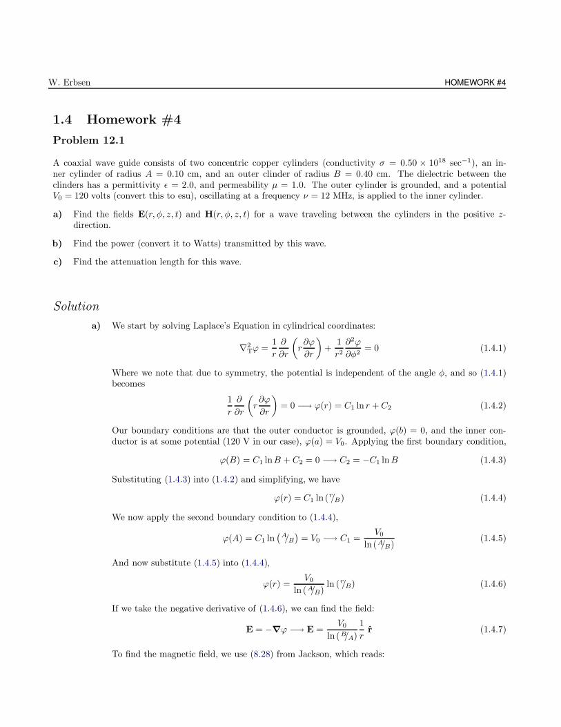
A coaxial wave guide consists of two concentric copper cylinders (conductivity σ = 0.50 × 10¹⁸ sec−1), an in-ner cylinder of radius A = 0.10 cm, and an outer clinder of radius B = 0.40 cm. The dielectric between theclinders has a permittivity ε = 2.0, and permeability µ = 1.0. The outer cylinder is grounded, and a potentialV0 = 120 volts (convert this to esu), oscillating at a frequency ν = 12 MHz, is applied to the inner cylinder.
a) Find the fields E(r, φ, z, t) and H(r, φ, z, t) for a wave traveling between the cylinders in the positive z-direction.
b) Find the power (convert it to Watts) transmitted by this wave.
c) Find the attenuation length for this wave.
Solution
a) We start by solving Laplace’s Equation in cylindrical coordinates:
∇2Tϕ =
1
r
∂
∂r
(r∂ϕ
∂r
)+
1
r2∂2ϕ
∂φ2= 0 (1.4.1)
Where we note that due to symmetry, the potential is independent of the angle φ, and so (1.4.1)becomes
1
r
∂
∂r
(r∂ϕ
∂r
)= 0 −→ ϕ(r) = C1 ln r +C2 (1.4.2)
Our boundary conditions are that the outer conductor is grounded, ϕ(b) = 0, and the inner con-ductor is at some potential (120 V in our case), ϕ(a) = V0. Applying the first boundary condition,
ϕ(B) = C1 lnB + C2 = 0 −→ C2 = −C1 lnB (1.4.3)
Substituting (1.4.3) into (1.4.2) and simplifying, we have
ϕ(r) = C1 ln (r/B) (1.4.4)
We now apply the second boundary condition to (1.4.4),
ϕ(A) = C1 ln(
A/B)
= V0 −→ C1 =V0
ln (A/B)(1.4.5)
And now substitute (1.4.5) into (1.4.4),
ϕ(r) =V0
ln (A/B)ln (r/B) (1.4.6)
If we take the negative derivative of (1.4.6), we can find the field:
E = −∇ϕ −→ E =V0
ln (B/A)
1
rr (1.4.7)
To find the magnetic field, we use (8.28) from Jackson, which reads:
CHAPTER 1: ELECTRODYNAMICS II 35
H = ±√µε z × E
Using (8.28), the magnetic field becomes
H =√µε
V0
ln (B/A)
1
rz × r −→ H =
√µε
V0
ln (B/A)
1
rφ (1.4.8)
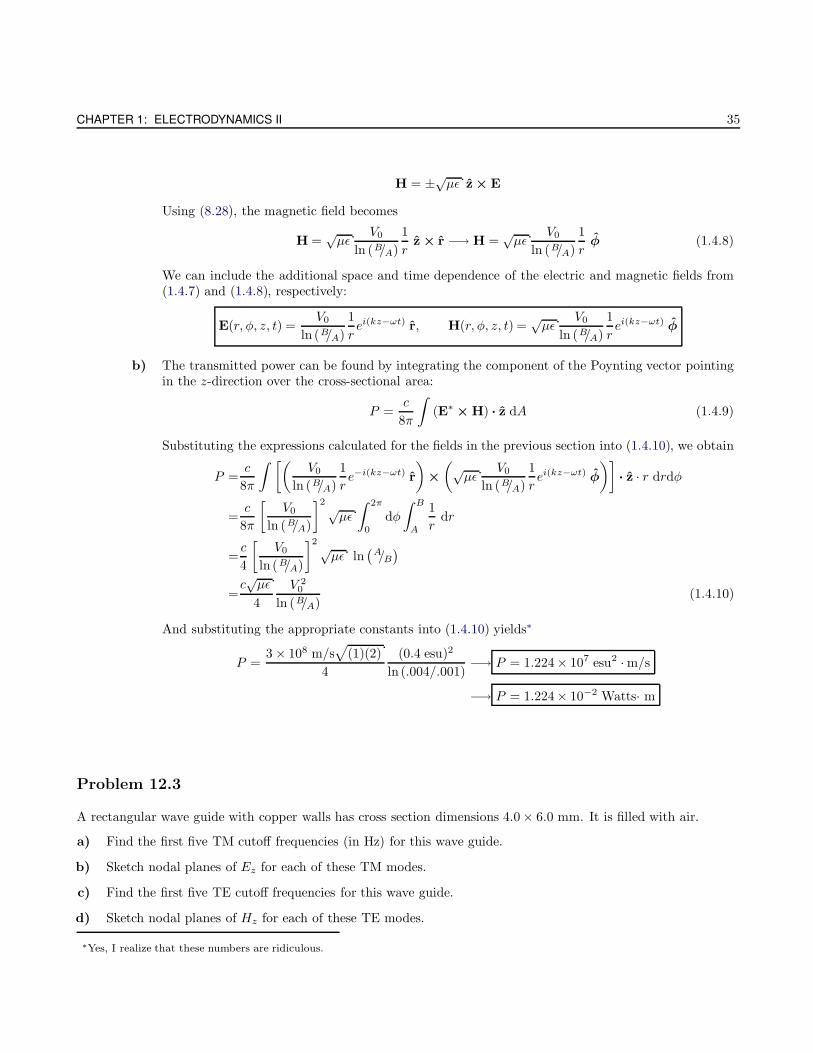
We can include the additional space and time dependence of the electric and magnetic fields from(1.4.7) and (1.4.8), respectively:
E(r, φ, z, t) =V0
ln (B/A)
1
rei(kz−ωt) r, H(r, φ, z, t) =
√µε
V0
ln (B/A)
1
rei(kz−ωt) φ
b) The transmitted power can be found by integrating the component of the Poynting vector pointingin the z-direction over the cross-sectional area:
P =c
8π
∫(E∗
× H) · z dA (1.4.9)
Substituting the expressions calculated for the fields in the previous section into (1.4.10), we obtain
P =c
8π
∫ [(V0
ln (B/A)
1
re−i(kz−ωt) r
)×
(√µε
V0
ln (B/A)
1
rei(kz−ωt) φ
)]· z · r drdφ
=c
8π
[V0
ln (B/A)
]2 √µε
∫ 2π
0
dφ
∫ B
A
1
rdr
=c
4
[V0
ln (B/A)
]2 √µε ln
(A/B)
=c√µε
4
V 20
ln (B/A)(1.4.10)
And substituting the appropriate constants into (1.4.10) yields∗
P =3 × 10⁸ m/s
√(1)(2)
4
(0.4 esu)2
ln (.004/.001)−→ P = 1.224× 10⁷ esu2 ·m/s
−→ P = 1.224× 10⁻² Watts· m
Problem 12.3
A rectangular wave guide with copper walls has cross section dimensions 4.0× 6.0 mm. It is filled with air.
a) Find the first five TM cutoff frequencies (in Hz) for this wave guide.
b) Sketch nodal planes of Ez for each of these TM modes.
c) Find the first five TE cutoff frequencies for this wave guide.
d) Sketch nodal planes of Hz for each of these TE modes.
∗Yes, I realize that these numbers are ridiculous.
W. Erbsen HOMEWORK #4
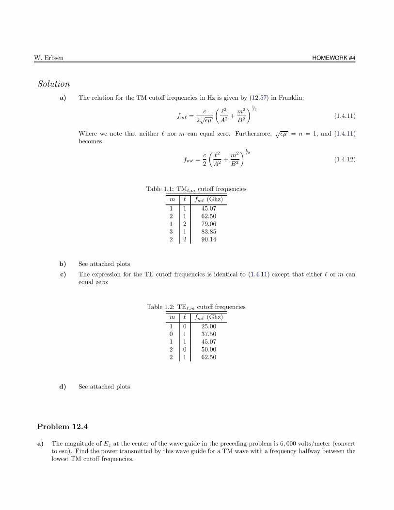
Solution
a) The relation for the TM cutoff frequencies in Hz is given by (12.57) in Franklin:
fm` =c
2√εµ
(`2
A2+m2
B2
) 1/2
(1.4.11)
Where we note that neither ` nor m can equal zero. Furthermore,√εµ = n = 1, and (1.4.11)
becomes
fm` =c
2
(`2
A2+m2
B2
) 1/2
(1.4.12)
Table 1.1: TM`,m cutoff frequencies
m ` fm` (Ghz)
1 1 45.072 1 62.501 2 79.063 1 83.852 2 90.14
b) See attached plots
c) The expression for the TE cutoff frequencies is identical to (1.4.11) except that either ` or m canequal zero:
Table 1.2: TE`,m cutoff frequencies
m ` fm` (Ghz)
1 0 25.000 1 37.501 1 45.072 0 50.002 1 62.50
d) See attached plots
Problem 12.4
a) The magnitude of Ez at the center of the wave guide in the preceding problem is 6, 000 volts/meter (convertto esu). Find the power transmitted by this wave guide for a TM wave with a frequency halfway between thelowest TM cutoff frequencies.
CHAPTER 1: ELECTRODYNAMICS II 37
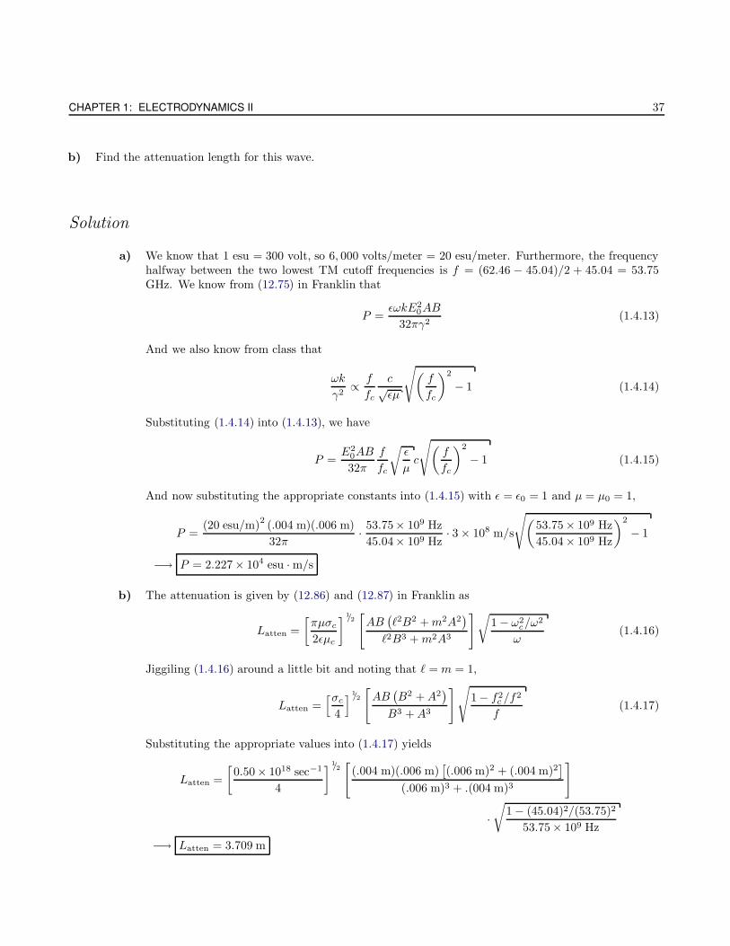
b) Find the attenuation length for this wave.
Solution
a) We know that 1 esu = 300 volt, so 6, 000 volts/meter = 20 esu/meter. Furthermore, the frequencyhalfway between the two lowest TM cutoff frequencies is f = (62.46 − 45.04)/2 + 45.04 = 53.75GHz. We know from (12.75) in Franklin that
P =εωkE2
0AB
32πγ2(1.4.13)
And we also know from class that
ωk
γ2∝ f
fc
c√εµ
√(f
fc
)2
− 1 (1.4.14)
Substituting (1.4.14) into (1.4.13), we have
P =E2
0AB
32π
f
fc
√ε
µc
√(f
fc
)2
− 1 (1.4.15)
And now substituting the appropriate constants into (1.4.15) with ε = ε0 = 1 and µ = µ0 = 1,
P =(20 esu/m)
2(.004 m)(.006 m)
32π· 53.75× 109 Hz
45.04× 109 Hz· 3 × 108 m/s
√(53.75× 10⁹ Hz
45.04× 10⁹ Hz
)2
− 1
−→ P = 2.227× 10⁴ esu · m/s
b) The attenuation is given by (12.86) and (12.87) in Franklin as
Latten =
[πµσc
2εµc
]1/2[AB
(`2B2 +m2A2
)
`2B3 +m2A3
]√1 − ω2
c/ω2
ω(1.4.16)
Jiggiling (1.4.16) around a little bit and noting that ` = m = 1,
Latten =[σc
4
] 1/2
[AB
(B2 +A2
)
B3 +A3
]√1− f2
c /f2
f(1.4.17)
Substituting the appropriate values into (1.4.17) yields
Latten =
[0.50× 10¹⁸ sec−1
4
]1/2[
(.004 m)(.006 m)[(.006 m)2 + (.004 m)2
]
(.006 m)3 + .(004 m)3
]
·√
1 − (45.04)2/(53.75)2
53.75× 10⁹ Hz
−→ Latten = 3.709 m
W. Erbsen HOMEWORK #4
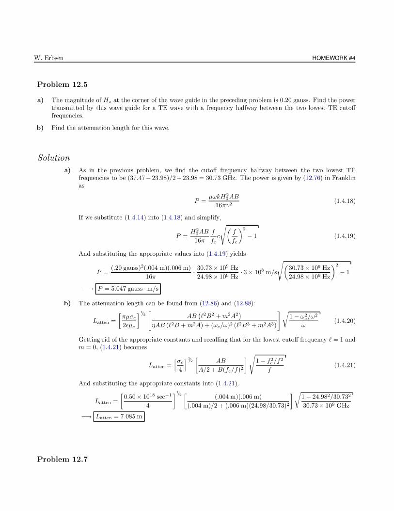
Problem 12.5
a) The magnitude of Hz at the corner of the wave guide in the preceding problem is 0.20 gauss. Find the powertransmitted by this wave guide for a TE wave with a frequency halfway between the two lowest TE cutofffrequencies.
b) Find the attenuation length for this wave.
Solution
a) As in the previous problem, we find the cutoff frequency halfway between the two lowest TEfrequencies to be (37.47− 23.98)/2+23.98 = 30.73 GHz. The power is given by (12.76) in Franklinas
P =µωkH2
0AB
16πγ2(1.4.18)
If we substitute (1.4.14) into (1.4.18) and simplify,
P =H2
0AB
16π
f
fcc
√(f
fc
)2
− 1 (1.4.19)
And substituting the appropriate values into (1.4.19) yields
P =(.20 gauss)2(.004 m)(.006 m)
16π· 30.73× 109 Hz
24.98× 109 Hz· 3 × 108 m/s
√(30.73× 10⁹ Hz
24.98× 10⁹ Hz
)2
− 1
−→ P = 5.047 gauss · m/s
b) The attenuation length can be found from (12.86) and (12.88):
Latten =
[πµσc
2εµc
] 1/2[
AB(`2B2 +m2A2
)
ηAB (`2B +m2A) + (ωc/ω)2 (`2B3 +m2A3)
]√1 − ω2
c/ω2
ω(1.4.20)
Getting rid of the appropriate constants and recalling that for the lowest cutoff frequency ` = 1 andm = 0, (1.4.21) becomes
Latten =[σc
4
] 1/2[
AB
A/2 + B(fc/f)2
]√1 − f2
c /f2
f(1.4.21)
And substituting the appropriate constants into (1.4.21),
Latten =
[0.50× 10¹⁸ sec−1
4
]1/2 [ (.004 m)(.006 m)
(.004 m)/2 + (.006 m)(24.98/30.73)2
]√1 − 24.982/30.732
30.73× 10⁹ GHz
−→ Latten = 7.085 m
Problem 12.7
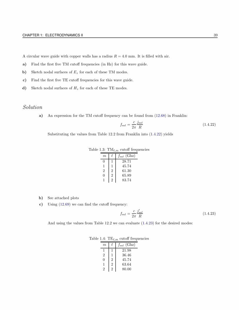
CHAPTER 1: ELECTRODYNAMICS II 39
A circular wave guide with copper walls has a radius R = 4.0 mm. It is filled with air.
a) Find the first five TM cutoff frequencies (in Hz) for this wave guide.
b) Sketch nodal surfaces of Ez for each of these TM modes.
c) Find the first five TE cutoff frequencies for this wave guide.
d) Sketch nodal surfaces of Hz for each of these TE modes.
Solution
a) An expression for the TM cutoff frequency can be found from (12.68) in Franklin:
fm` =c
2π
jm`
R(1.4.22)
Substituting the values from Table 12.2 from Franklin into (1.4.22) yields
Table 1.3: TM`,m cutoff frequencies
m ` fm` (Ghz)
0 1 28.711 1 45.742 2 61.300 2 65.891 2 83.74
b) See attached plots
c) Using (12.69) we can find the cutoff frequency:
fm` =c
2π
j′m`
R(1.4.23)
And using the values from Table 12.2 we can evaluate (1.4.23) for the desired modes:
Table 1.4: TE`,m cutoff frequencies
m ` fm` (Ghz)
1 1 21.982 1 36.460 2 45.741 2 63.642 2 80.00
W. Erbsen HOMEWORK #5
d) See attached plots
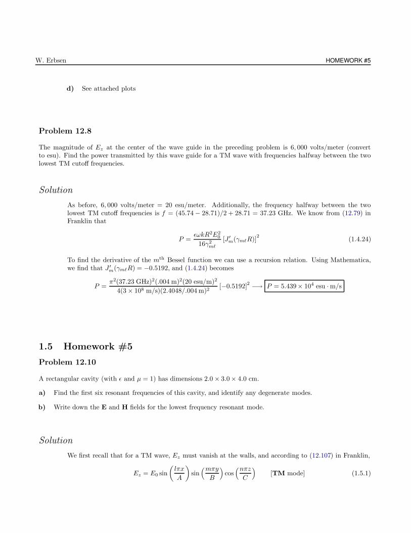
Problem 12.8
The magnitude of Ez at the center of the wave guide in the preceding problem is 6, 000 volts/meter (convertto esu). Find the power transmitted by this wave guide for a TM wave with frequencies halfway between the twolowest TM cutoff frequencies.
Solution
As before, 6, 000 volts/meter = 20 esu/meter. Additionally, the frequency halfway between the twolowest TM cutoff frequencies is f = (45.74 − 28.71)/2 + 28.71 = 37.23 GHz. We know from (12.79) inFranklin that
P =εωkR2E2
0
16γ2m`
[J ′m(γm`R)]
2(1.4.24)
To find the derivative of the mth Bessel function we can use a recursion relation. Using Mathematica,we find that J ′
m(γm`R) = −0.5192, and (1.4.24) becomes
P =π2(37.23 GHz)2(.004 m)2(20 esu/m)2
4(3 × 10⁸ m/s)(2.4048/.004 m)2[−0.5192]
2 −→ P = 5.439× 10⁴ esu ·m/s
1.5 Homework #5
Problem 12.10
A rectangular cavity (with ε and µ = 1) has dimensions 2.0 × 3.0× 4.0 cm.
a) Find the first six resonant frequencies of this cavity, and identify any degenerate modes.
b) Write down the E and H fields for the lowest frequency resonant mode.
Solution
We first recall that for a TM wave, Ez must vanish at the walls, and according to (12.107) in Franklin,
Ez = E0 sin
(lπx
A
)sin(mπy
B
)cos(nπzC
)[TM mode] (1.5.1)
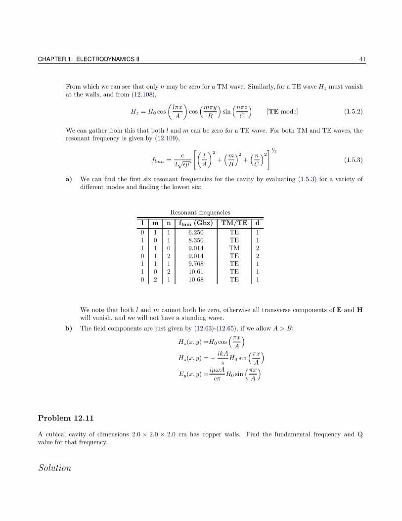
CHAPTER 1: ELECTRODYNAMICS II 41
From which we can see that only n may be zero for a TM wave. Similarly, for a TE wave Hz must vanishat the walls, and from (12.108),
Hz = H0 cos
(lπx
A
)cos(mπyB
)sin(nπzC
)[TE mode] (1.5.2)
We can gather from this that both l and m can be zero for a TE wave. For both TM and TE waves, theresonant frequency is given by (12.109),
flmn =c
2√εµ
[(l
A
)2
+(mB
)2
+( nC
)2] 1/2
(1.5.3)
a) We can find the first six resonant frequencies for the cavity by evaluating (1.5.3) for a variety ofdifferent modes and finding the lowest six:
Resonant frequencies
l m n flmn (Ghz) TM/TE d
0 1 1 6.250 TE 11 0 1 8.350 TE 11 1 0 9.014 TM 20 1 2 9.014 TE 21 1 1 9.768 TE 11 0 2 10.61 TE 10 2 1 10.68 TE 1
We note that both l and m cannot both be zero, otherwise all transverse components of E and Hwill vanish, and we will not have a standing wave.
b) The field components are just given by (12.63)-(12.65), if we allow A > B:
Hz(x, y) =H0 cos(πxA
)
Hz(x, y) = − ikA
πH0 sin
(πxA
)
Ey(x, y) =iµωA
cπH0 sin
(πxA
)
Problem 12.11
A cubical cavity of dimensions 2.0 × 2.0 × 2.0 cm has copper walls. Find the fundamental frequency and Qvalue for that frequency.
Solution
W. Erbsen HOMEWORK #5
From (1.5.3),
flmn =c
2√εµ
[(l
.02 m
)2
+( m
.02 m
)2
+( n
0.02 m
)2] 1/2
−→ f110 = f101 = f011 = 10.61 GHz
The derivation for the expression for the Q value is found in the next problem, and is given by (1.5.21)as
Q =4πL
c
√fσc
µc(1.5.4)
Where “L” is the length of each side of the cavity. The conductivity of copper is given by σc = 5.96 ·1017 Ω−1 · m, while we let µc = 1. Accordingly, (1.5.4) leads to Q ≈ 0.2107 .
Problem 12.12
“And they shall make an ark of acacia-wood: two cubits and a half shall be the length thereof, and a cubitand a half the breadth thereof, and a cubit and a half the height thereof. And thou shalt overlay it with puregold.” (Exodus XXV, 10:11). Find the fundamental resonant frequency and a half width for this biblical cavity.Use the length from your fingertip to your elbow as a measure of a biblical cubit.
Solution
The length from my elbow to my beefy fingertip is ∼ 0.5 m, so the dimensions of our cavity are A = 1.25m, B = 0.75 m, and C = 0.75 m. The fundamental frequency may be readily deduced from (1.5.3):
flmn =c
2√εµ
[(l
1.25 m
)2
+( m
0.75 m
)2
+( n
0.75 m
)2] 1/2
−→ f110 = f101 = 0.2330 GHz
Which is clearly degenerate. We can see that f110 corresponds to a TM mode, while f101 corresponds toa TE mode. The half width is found by dividing (12.131) by a factor of 2,
Γ =ω0
2Q(1.5.5)
While the Q factor is given by (12.125) as
Q = − ωU
dU/dt(1.5.6)
Where we know that
dU
dt= − c
8π
√ωµc
8πσc
∫|Hsurface|2dA (1.5.7)
And if we recall from (1.5.1) and (1.5.2),
CHAPTER 1: ELECTRODYNAMICS II 43
Ez =E0 sin
(lπx
A
)sin(mπyB
)cos(nπzC
)(1.5.8)
Hz =H0 cos
(lπx
A
)cos(mπyB
)sin(nπzC
)(1.5.9)
For the TM mode, we know that l = 1, m = 1 and n = 0, and (1.5.8) becomes
Ez = E0 sin(πxA
)sin(πyB
)(1.5.10)
And similarly, for the TE mode, we recall that l = 1, m = 0 and l = 1, and (1.5.9) becomes
Hz = H0 cos(πxA
)sin(πzC
)(1.5.11)
We know that Hsurface will be a linear combination of both fields, so we can go ahead and evaluate themodulus squared:
|Hsurface|2 =[E0 sin
(πxA
)sin(πyB
)+H0 cos
(πxA
)sin(πzC
)]2
=E20 sin2
(πxA
)sin2
(πyB
)
︸ ︷︷ ︸ψI
+H20 cos2
(πxA
)sin2
(πzC
)
︸ ︷︷ ︸ψII
+ 2E0H0 sin(πxA
)sin(πyB
)cos(πxA
)sin(πzC
)
︸ ︷︷ ︸ψIII
=E20ψI +H2
0ψII + 2E0H0ψIII (1.5.12)
Instead of directly substituting (1.5.12) into (1.5.7), we can go ahead and integrate ψI , ψII and ψIII
separately over space and then combine them later to avoid some of the mess. We first recall the followingnifty trig identities:
sin2 x =1
2(1 − cos(2x)) cos2 x =
1
2(1 + cos(2x))
Using these, we first evaluate ψI ,
∫ψIdA =
∫ A
0
sin2(πxA
)dx ·
∫ B
0
sin2(πyB
)dy
=1
4
∫ A
0
[1 − cos
(2πx
A
)]dx ·
∫ B
0
[1 − cos
(2πy
B
)]dy
=1
4
[∫ A
0
dx−∫ A
0
cos
(2πx
A
)dx
]·[∫ B
0
dy −∫ B
0
cos
(2πy
B
)dy
]
=1
4
[A− A
2π
[sin
(2πx
A
)∣∣∣∣A
0
]·[B − B
2π
[sin
(2πy
B
)∣∣∣∣B
0
]
=AB
4(1.5.13)
And now doing the same for ψII ,
W. Erbsen HOMEWORK #5
∫ψIIdA =
∫ A
0
cos2(πxA
)dx ·
∫ C
0
sin2(πzC
)dz
=1
4
∫ A
0
[1 + cos
(2πx
A
)]dx ·
∫ C
0
[1 − cos
(2πz
C
)]dz
=1
4
[A +
∫ A
0
cos
(2πx
A
)dx
]·[C −
∫ C
0
cos
(2πz
C
)dz
]
=1
4
[A +
A
2π
[sin
(2πx
A
)∣∣∣∣A
0
]·[C − C
2π
[sin
(2πz
C
)∣∣∣∣C
0
]
=AC
4(1.5.14)
And now for ψIII ,
∫ψIIIdA =
∫ A
0
sin(πxA
)cos(πxA
)dx
︸ ︷︷ ︸=⇒ 0
·∫ B
0
sin(πyB
)dy ·
∫ C
0
sin(πzC
)dz = 0 (1.5.15)
Using (1.5.13)-(1.5.15), we can now evaluate (1.5.7):
dU
dt= − c
8π
√ωµc
8πσc
[E2
0
AB
4+H2
0
AC
4
]
= − c
64π
√fµc
σcA[E2
0B +H20C]
(1.5.16)
We now find the energy within the cavity, U , using (12.121):
U =
(εE2
0 + µH20
)ABC
32π
[(l/A)
2+ (m/B)
2+ (n/C)
2
(l/A)2
+ (m/B)2
](1.5.17)
If we take the frequency for the TM mode we let l = 1, m = 1, and n = 0, and (1.5.17) becomes
U =
(εE2
0 + µH20
)ABC
32π(1.5.18)
We now recall that ε = µ = 1 and B = C, so (1.5.18) becomes
U =
(E2
0 +H20
)AB2
32π(1.5.19)
Making the same assumptions for (1.5.16) yields
dU
dt= − c
64π
√fµc
σcAB
[E2
0 +H20
](1.5.20)
Now substituting (1.5.19) and (1.5.20) into (1.5.6) yields
Q = − 2πf · AB2
32π
(E2
0 +H20
)· −64π
c
√σc
fµc
1
AB (E20 +H2
0)
CHAPTER 1: ELECTRODYNAMICS II 45
=4πB
c
√fσc
µc(1.5.21)
The conductivity of gold can be found on p. 286 of Griffiths to be σc = 4.525 × 10⁷ Ω−1 · m. Takingµc = 1, (1.5.21) becomes
Q =4π(0.75 m)
(3 × 10⁸ m/s)
√(0.233× 10⁹ Hz)(4.525× 10⁷ Ω−1 ·m −→ Q ≈ 3.226 (1.5.22)
Substituting (1.5.22) into (1.5.5),
Γ =πf0Q
−→ Γ = 0.2269 GHz
It is clear that this answer does not make sense, if we compare it to the resonant frequency found inthe first part of the problem. I repeated the latter part using Mathematica, which yielded a half width
of Γ = .03612 GHz . Please see attached Mathematica printout for details.
Problem 12.13
A circular cavity (with ε and µ = 1) has a radius R = 2.0 cm, and a length L = 3.0 cm.
a) Find the first six resonant frequencies of this cavity, and identify the type (TM or TE) of mode.
b) Sketch nodal surfaces for each of these six modes.
Solution
a) The relation for the resonant frequencies for both TM and TE modes is given by (12.112),
flmn =c
2√εµ
[(jml
πR
)2
+(nL
)2] 1/2
[TM mode] (1.5.23)
f ′lmn =c
2√εµ
[(j′ml
πR
)2
+(nL
)2] 1/2
[TE mode] (1.5.24)
The calculated values are displayed in the following table (next page):
b) Please see attached plots.
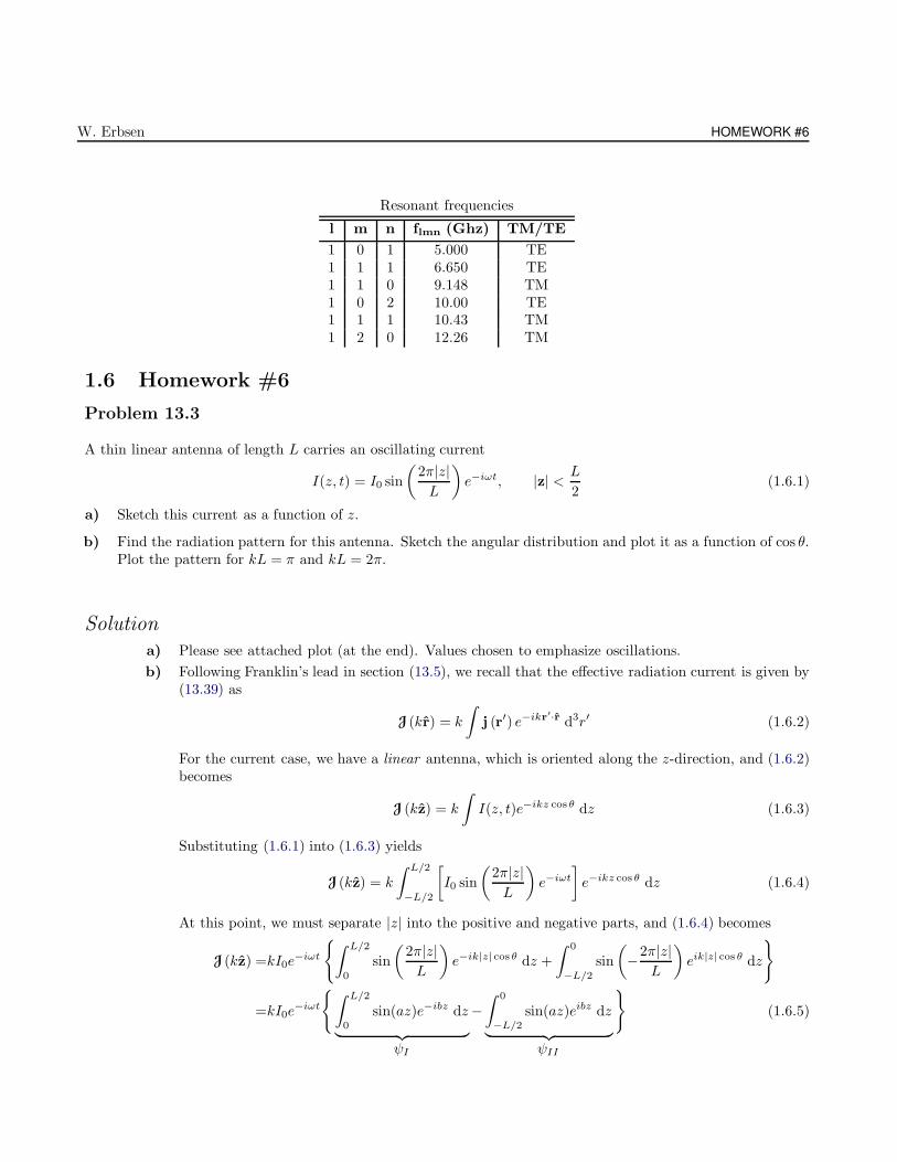
W. Erbsen HOMEWORK #6
Resonant frequencies
l m n flmn (Ghz) TM/TE
1 0 1 5.000 TE1 1 1 6.650 TE1 1 0 9.148 TM1 0 2 10.00 TE1 1 1 10.43 TM1 2 0 12.26 TM
1.6 Homework #6
Problem 13.3
A thin linear antenna of length L carries an oscillating current
I(z, t) = I0 sin
(2π|z|L
)e−iωt, |z| < L
2(1.6.1)
a) Sketch this current as a function of z.
b) Find the radiation pattern for this antenna. Sketch the angular distribution and plot it as a function of cos θ.Plot the pattern for kL = π and kL = 2π.
Solution
a) Please see attached plot (at the end). Values chosen to emphasize oscillations.
b) Following Franklin’s lead in section (13.5), we recall that the effective radiation current is given by(13.39) as
J (kr) = k
∫j (r′) e−ikr′·r d3r′ (1.6.2)
For the current case, we have a linear antenna, which is oriented along the z-direction, and (1.6.2)becomes
J (kz) = k
∫I(z, t)e−ikz cos θ dz (1.6.3)
Substituting (1.6.1) into (1.6.3) yields
J (kz) = k
∫ L/2
−L/2
[I0 sin
(2π|z|L
)e−iωt
]e−ikz cos θ dz (1.6.4)
At this point, we must separate |z| into the positive and negative parts, and (1.6.4) becomes
J (kz) =kI0e−iωt
∫ L/2
0
sin
(2π|z|L
)e−ik|z| cos θ dz +
∫ 0
−L/2
sin
(−2π|z|
L
)eik|z| cos θ dz
=kI0e−iωt
∫ L/2
0
sin(az)e−ibz dz
︸ ︷︷ ︸ψI
−∫ 0
−L/2
sin(az)eibz dz
︸ ︷︷ ︸ψII
(1.6.5)
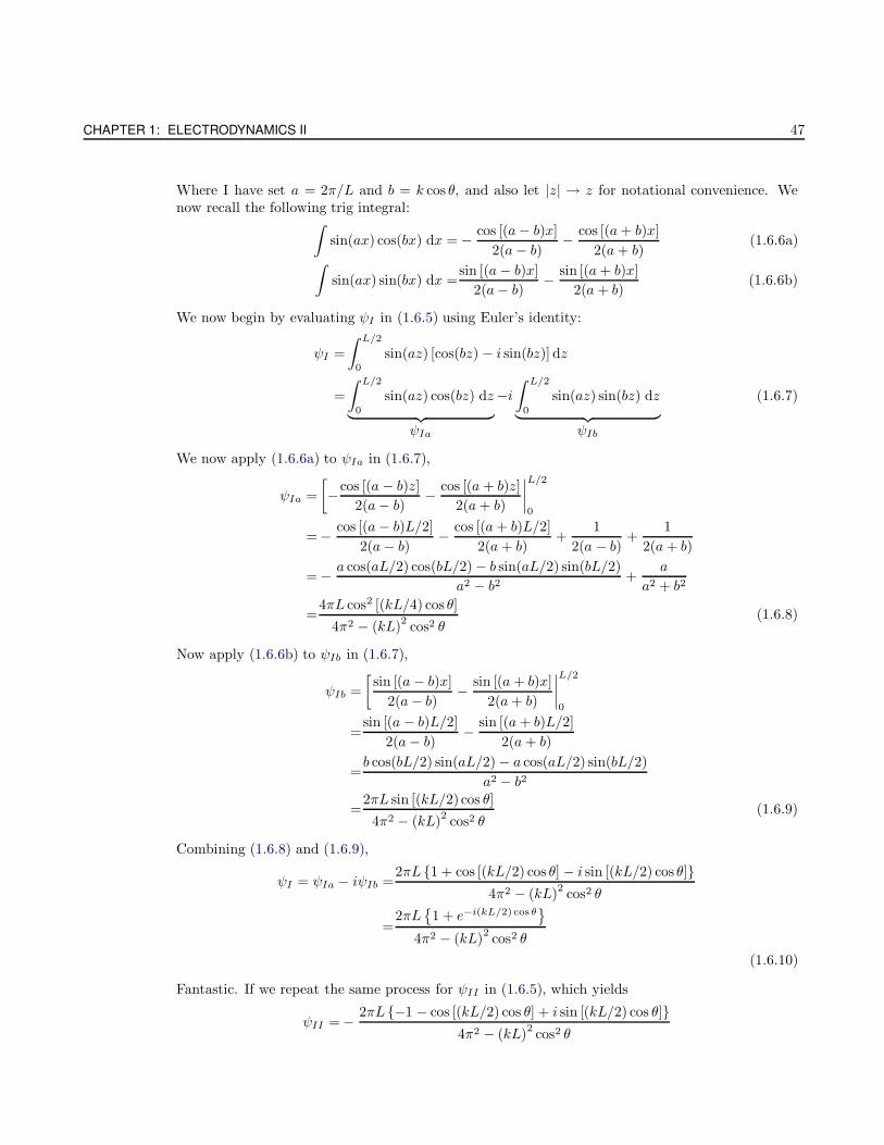
CHAPTER 1: ELECTRODYNAMICS II 47
Where I have set a = 2π/L and b = k cos θ, and also let |z| → z for notational convenience. Wenow recall the following trig integral:
∫sin(ax) cos(bx) dx = − cos [(a− b)x]
2(a− b)− cos [(a+ b)x]
2(a+ b)(1.6.6a)
∫sin(ax) sin(bx) dx =
sin [(a− b)x]
2(a− b)− sin [(a+ b)x]
2(a + b)(1.6.6b)
We now begin by evaluating ψI in (1.6.5) using Euler’s identity:
ψI =
∫ L/2
0
sin(az) [cos(bz) − i sin(bz)] dz
=
∫ L/2
0
sin(az) cos(bz) dz
︸ ︷︷ ︸ψIa
−i∫ L/2
0
sin(az) sin(bz) dz
︸ ︷︷ ︸ψIb
(1.6.7)
We now apply (1.6.6a) to ψIa in (1.6.7),
ψIa =
[−cos [(a − b)z]
2(a− b)− cos [(a + b)z]
2(a+ b)
∣∣∣∣L/2
0
= − cos [(a− b)L/2]
2(a− b)− cos [(a+ b)L/2]
2(a+ b)+
1
2(a − b)+
1
2(a+ b)
= − a cos(aL/2) cos(bL/2) − b sin(aL/2) sin(bL/2)
a2 − b2+
a
a2 + b2
=4πL cos2 [(kL/4) cos θ]
4π2 − (kL)2cos2 θ
(1.6.8)
Now apply (1.6.6b) to ψIb in (1.6.7),
ψIb =
[sin [(a − b)x]
2(a− b)− sin [(a + b)x]
2(a+ b)
∣∣∣∣L/2
0
=sin [(a − b)L/2]
2(a− b)− sin [(a+ b)L/2]
2(a+ b)
=b cos(bL/2) sin(aL/2) − a cos(aL/2) sin(bL/2)
a2 − b2
=2πL sin [(kL/2) cos θ]
4π2 − (kL)2cos2 θ
(1.6.9)
Combining (1.6.8) and (1.6.9),
ψI = ψIa − iψIb =2πL 1 + cos [(kL/2) cos θ] − i sin [(kL/2) cos θ]
4π2 − (kL)2cos2 θ
=2πL
1 + e−i(kL/2) cos θ
4π2 − (kL)2cos2 θ
(1.6.10)
Fantastic. If we repeat the same process for ψII in (1.6.5), which yields
ψII = − 2πL −1 − cos [(kL/2) cos θ] + i sin [(kL/2) cos θ]4π2 − (kL)
2cos2 θ
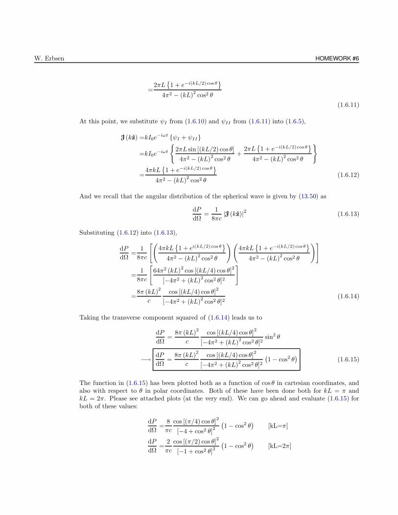
W. Erbsen HOMEWORK #6
=2πL
1 + e−i(kL/2)cos θ
4π2 − (kL)2 cos2 θ
(1.6.11)
At this point, we substitute ψI from (1.6.10) and ψII from (1.6.11) into (1.6.5),
J (kz) =kI0e−iωt ψI + ψII
=kI0e−iωt
2πL sin [(kL/2) cos θ]
4π2 − (kL)2cos2 θ
+2πL
1 + e−i(kL/2)cos θ
4π2 − (kL)2cos2 θ
=4πkL
1 + e−i(kL/2) cos θ
4π2 − (kL)2cos2 θ
(1.6.12)
And we recall that the angular distribution of the spherical wave is given by (13.50) as
dP
dΩ=
1
8πc|J (kz)|2 (1.6.13)
Substituting (1.6.12) into (1.6.13),
dP
dΩ=
1
8πc
[(4πkL
1 + ei(kL/2)cos θ
4π2 − (kL)2cos2 θ
)(4πkL
1 + e−i(kL/2) cos θ
4π2 − (kL)2cos2 θ
)]
=1
8πc
[64π2 (kL)
2cos [(kL/4) cos θ]
2
[−4π2 + (kL)2cos2 θ]2
]
=8π (kL)
2
c
cos [(kL/4) cos θ]2
[−4π2 + (kL)2cos2 θ]2
(1.6.14)
Taking the transverse component squared of (1.6.14) leads us to
dP
dΩ=
8π (kL)2
c
cos [(kL/4) cos θ]2
[−4π2 + (kL)2cos2 θ]2
sin2 θ
−→ dP
dΩ=
8π (kL)2
c
cos [(kL/4) cos θ]2
[−4π2 + (kL)2cos2 θ]2
(1 − cos2 θ
)(1.6.15)
The function in (1.6.15) has been plotted both as a function of cos θ in cartesian coordinates, andalso with respect to θ in polar coordinates. Both of these have been done both for kL = π andkL = 2π. Please see attached plots (at the very end). We can go ahead and evaluate (1.6.15) forboth of these values:
dP
dΩ=
8
πc
cos [(π/4) cos θ]2
[−4 + cos2 θ]2
(1 − cos2 θ
)[kL=π]
dP
dΩ=
2
πc
cos [(π/2) cos θ]2
[−1 + cos2 θ]2(1 − cos2 θ
)[kL=2π]
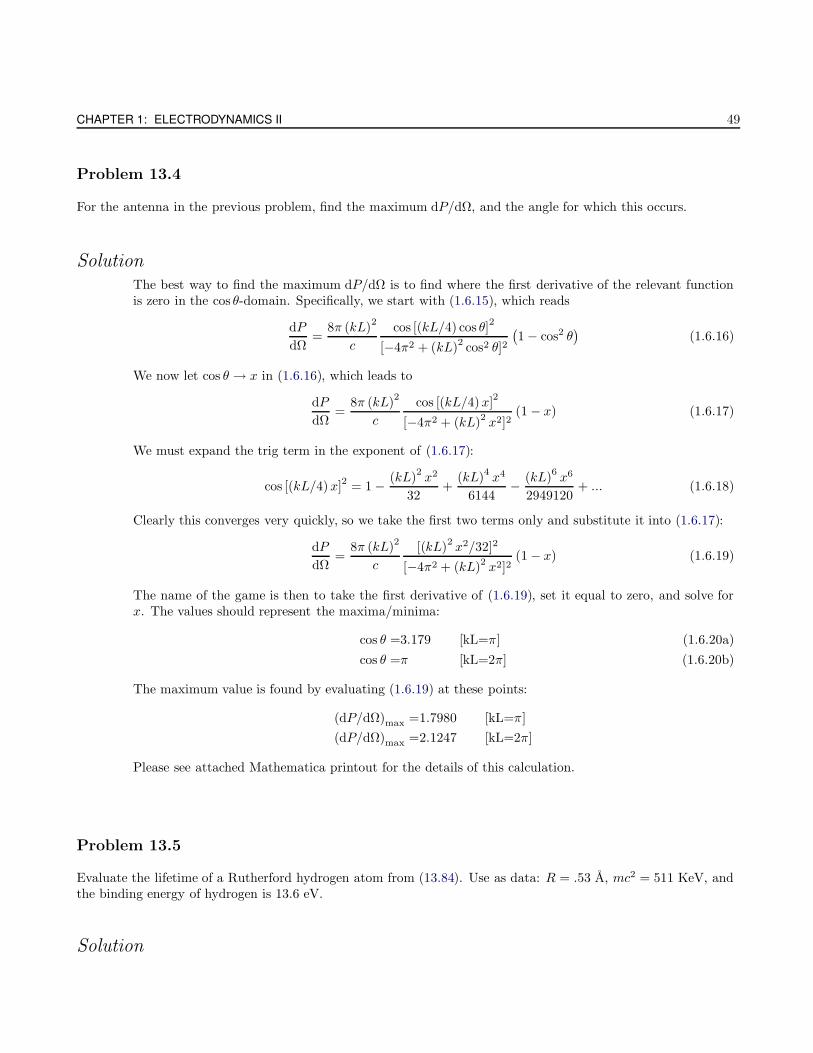
CHAPTER 1: ELECTRODYNAMICS II 49
Problem 13.4
For the antenna in the previous problem, find the maximum dP/dΩ, and the angle for which this occurs.
Solution
The best way to find the maximum dP/dΩ is to find where the first derivative of the relevant functionis zero in the cos θ-domain. Specifically, we start with (1.6.15), which reads
dP
dΩ=
8π (kL)2
c
cos [(kL/4) cos θ]2
[−4π2 + (kL)2 cos2 θ]2
(1 − cos2 θ
)(1.6.16)
We now let cos θ → x in (1.6.16), which leads to
dP
dΩ=
8π (kL)2
c
cos [(kL/4)x]2
[−4π2 + (kL)2 x2]2(1 − x) (1.6.17)
We must expand the trig term in the exponent of (1.6.17):
cos [(kL/4)x]2 = 1 − (kL)2x2
32+
(kL)4x4
6144− (kL)
6x6
2949120+ ... (1.6.18)
Clearly this converges very quickly, so we take the first two terms only and substitute it into (1.6.17):
dP
dΩ=
8π (kL)2
c
[(kL)2 x2/32]2
[−4π2 + (kL)2 x2]2(1 − x) (1.6.19)
The name of the game is then to take the first derivative of (1.6.19), set it equal to zero, and solve forx. The values should represent the maxima/minima:
cos θ =3.179 [kL=π] (1.6.20a)
cos θ =π [kL=2π] (1.6.20b)
The maximum value is found by evaluating (1.6.19) at these points:
(dP/dΩ)max =1.7980 [kL=π]
(dP/dΩ)max =2.1247 [kL=2π]
Please see attached Mathematica printout for the details of this calculation.
Problem 13.5
Evaluate the lifetime of a Rutherford hydrogen atom from (13.84). Use as data: R = .53 A, mc2 = 511 KeV, andthe binding energy of hydrogen is 13.6 eV.
Solution
W. Erbsen HOMEWORK #6
We begin with (13.84), which I will convert to SI units, in part by following the same logic as in thefollowing problem.
T =R
4c
[mc2
e2/R
]2
=cR
4
[mc
e2/R
]2
=cR3
4
[mce2
]2
=cR3
[2πε0mc
e2
]2(1.6.21)
The appropriate constants are
c =2.998× 10¹⁰ m/s
e =1.6023× 10¹⁰ C
R =0.529× 10⁻¹⁰ m
m =9.109× 10⁻³¹ Kg
ε0 =8.854× 10⁻¹² F/m
Plugging all of these into (1.6.21), we have
T =(2.998× 10¹⁰ m/s
) (0.529× 10⁻¹⁰ m
)3
·[
2π(8.854× 10⁻¹² F/m
) (9.109× 10⁻³¹ Kg
) (2.998× 10¹⁰ m/s
)
(1.6023× 10¹⁰ C)2
]2
−→ T ≈ 1.322× 10⁻¹¹ sec
Problem 13.6
Consider a model of the hydrogen atom as a heavy positive proton, surrounded by a sphere of radius R, witha uniform charge and mass density, having a total charge and mass of an electron.
a) Show that the angular frequency of oscillation for this atom (with amplitude A ≤ R) is
ω =
[(e2/R)
mc2
] 1/2 c
R(1.6.22)
b) Evaluate ω and the corresponding wavelength of radiation. (Use numerical values from the previous problem).
c) Find the oscillating electric dipole moment of this atom.
d) Find the total power radiated by this atom for A0 = R.
CHAPTER 1: ELECTRODYNAMICS II 51
e) Find the lifetime for exponential decay of the oscillation. Evaluate the lifetime in seconds.
Solution
a) We begin by equating Newton’s second law with Coulomb’s law,
F =mv2
r= mω2r =
1
4πε0
e2
r2−→ ω2r3 =
1
4πε0
e2
m(1.6.23)
The energy as a function of r is
E =T + V
=mv2
r− 1
4πε0
e2
r
=1
2
[1
4πε0
ε2
r
]− 1
4πε0
e2
r
= − 1
8πε0
e2
r(1.6.24)
To find the power loss we take the first derivative of (1.6.24),
dE
dt=
1
8πε0
e2
r2dr
dt(1.6.25)
The Lamor formula for radiation caused by an accelerating charge is given by (13.94)
P =2e2|a|2
3c3(1.6.26)
If we recognize that the power radiated can be thought of as the power lost, or the rate of energyleaving as a function of time, then we can say that:
dE
dt=
2e2|a|23c3
(1.6.27)
We now substitute in the acceleration for a charge circulating the proton,
dE
dt=
2e2(ω2r)2
3c3(1.6.28)
Substitute (1.6.23) into (1.6.28),
dE
dt=
2e2
3c3
[1
4πε0
e2
m
]2(1.6.29)
Equating (1.6.25) to (1.6.29),
1
8πε0
e2
r2dr
dt=
2e2
3c3
[1
4πε0
e2
m
]2−→dr
dt=
1
4πε0· 4e4
3m2c3
−→T = 4πε0 ·3m2c3
4e4
∫ 0
R
1
r2dr
−→T = 4πε0 ·m2c3
4e41
R3
W. Erbsen HOMEWORK #6
−→T = 4πε0R
4c
[mc2
e2/R
]2(1.6.30)
If we drop the factor of 4πε0, then (1.6.30) is the same as (13.84). Furthermore, we arrive at (13.161)by evaluating (1.6.23) at r = R:
ω2R3 =1
4πε0
e2
m−→ ω =
c
R
[1
4πε0
e2/R
mc2
](1.6.31)
If we let 4πε0 = 1 in (1.6.31), we are left with
ω =c
R
[e2/R
mc2
](1.6.32)
Which is identical to (1.6.22).
b) To evaluate ω, we simply use (1.6.23) and use the data from the previous problem:
ω =
[1
4πε0
e2
m
1
R3
]1/2
=
[1
4π (8.854× 10⁻¹² F/m)
(1.6023× 10¹⁰ C
)2
(9.109× 10⁻³¹ Kg)
1
(0.529× 10⁻¹⁰ m)3
] 1/2
(1.6.33)
−→ ω ≈ 4.496× 10¹⁶ rad
sec(1.6.34)
The wavelength of radiation will be given by:
λ =2πc
ω=
2π(2.998× 10¹⁰ m/s
)
4.496 Hz−→ λ ≈ 4.193× 10⁻⁸ m
c) The oscillating electric dipole moment is just the electric dipole moment, multiplied by a sinusoidaltime dependent frequency part:
p(t) =ed cos (ωt)
Where d in our case is equal to the separation of charge:
p(t) =eR cos (ωt) z (1.6.35)
Substituting in the appropriate values,
p(t) =(1.6023× 10¹⁰ C
) (0.529× 10⁻¹⁰ m
)cos (ωt) z −→ p(t) =
(8 × 10⁻³⁰ C · m
)cos (ωt) z
Where ω is of course given by (1.6.33).
d) The total power radiated is just (1.6.28):
P =2e2
(ω2r
)2
3c3
Putting in the numbers,
P =2(1.6023× 10¹⁰ C
)2 (4.496× 10¹⁶ rad/sec
)4 (0.529× 10⁻¹⁰ m
)2
3 (2.998× 10¹⁰ m/s)3 −→ P = 1.291× 10⁻⁷ Watts
CHAPTER 1: ELECTRODYNAMICS II 53
Problem 13.7
Find and sketch the absolute square of the Fourier transform of the step function in (13.95), and estimate itsspread in ω. (Use the first zero of the transform to estimate)
Solution
The step function in (13.95) reads
λ(x, t) =
q/L, |x− vt| < L/2
0, |x− vt| > L/2(1.6.36)
And now we recall that the functional form of the integral Fourier transform is
f(x, t) =
∫f(ω, t)eikx dk
A(k, t) =1
2π
∫f(x, t)e−ikx dx (1.6.37)
Where the integrals are to be taken over the appropriate range. In our case, we substitute (1.6.36) into(1.6.37), which yields
A(k, t) =1
2π
∫ L/2
−L/2
( qL
)e−ikx dx
=1
2π
( qL
) [−e
−ikx
ik
∣∣∣∣L/2
−L/2
=1
2π
( qL
) [−e−ikL/2 + eikL/2
ik
]
=q
π
sin (kL/2)
kL(1.6.38)
Taking the absolute square of (1.6.38) leads to
A(k, t) =q2
π2
sin2 (kL/2)
(kL)2 (1.6.39)
In order to estimate the spread of (1.6.39) in ω, we evaluate the function at the first zero:
q2
π2
sin2 (kL/2)
(kL)2 = 0 −→ kL = 2π −→ L
ω= 1 −→ ∆ω = 2L
W. Erbsen HOMEWORK #7
1.7 Homework #7
Problem 13.8
A beam of 2 KeV electrons is stopped in a distance of 0.01 cm.
a) Calculate the total energy of the radiation emitted by each electron (assume constant acceleration).
b) Find the ratio of the emitted energy to the initial electron energy. Use this ratio to find the radiated powerfor an x-ray machine with 300 Watts of power input to accelerate the electrons.
c) Calculate the maximum intensity of the radiation at a distance of 20 cm from the stopping target.
Solution
a) To find the total energy radiated by each electron, we first convert the initial kinetic energy of theelectrons (T ) from eV to Joules:
T = 2 × 103 eV · 1.602× 10−19 J
1 eV−→ T = 3.204× 10⁻¹⁶ J
We now recall that the kinetic is given by
T = 1/2mv2 −→ v =
√2T
m(1.7.1)
And, since we are told that the acceleration is constant, we can use one of the kinematic equationsof motion:
v2 = v2o + 2a∆x −→ a = − v2
o
2∆x(1.7.2)
If we take (1.7.1) and substitute it into (1.7.2) and put in the appropriate values,
a = −2T/m
2∆x⇒ − T
m∆x⇒ −
(3.204× 10⁻¹⁶ J
)
(9.109× 10⁻³¹ kg) (.01× 10−2 m)−→ a = −3.518× 10¹⁸ m/s
2
We can now find the power from the following expressions:
P =2e2|a|2
3c3[CGS] (1.7.3a)
P =e2|a|26πε0c3
[SI] (1.7.3b)
Where (1.7.3a) comes from (13.94) in Franklin, and (1.7.3b) comes from Wikipedia. Doing thecalculation in SI units first,
P =(1.602× 10⁻¹⁹ C)2(3.518× 10¹⁸ m/s
2)2
6π(8.854× 10⁻¹² F/m)(2.998× 108 m/s)3−→ P = 7.063× 10⁻¹⁷ Watts (1.7.4)
And doing the same in CGS units with (1.7.3a),
P =24.803× 10⁻¹⁰ StatC)2(3.518× 1020 cm/s
2)2
3(2.998× 1010 cm/s)3−→ P = 7.063× 10⁻¹⁰ erg/s (1.7.5)
CHAPTER 1: ELECTRODYNAMICS II 55
In order to find the energy emitted, we must find the time over which this happens. We again turnto the kinematic equations of motion:
v = vo + at −→ t = −voa
Substituting in the expression for vo from (1.7.1) into this yields
t = −√
2T/m
a⇒ −
√(2) (3.204× 10⁻¹⁶ J) / (9.109× 10⁻³¹ kg)
−3.518× 10¹⁸ m/s2 −→ t = 7.540× 10⁻¹² s
Now, if we recall that [power]=[energy]/[time], then we can find the energy by multiplying ourexpressions for power from (1.7.4) and (1.7.5), respectively by the time we just calculated:
E =(7.063× 10⁻¹⁷ Watts
) (7.540× 10⁻¹² s
)−→ E = 5.326× 10⁻²⁸ J
= 3.324× 10⁻⁹ eV[SI]
E =(7.063× 10⁻¹⁰ erg/s
) (7.540× 10⁻¹² s
)−→ E = 5.326× 10⁻²¹ erg [CGS]
b) We find the ratio of the energy emitted to the incident energy (T ′/T ) simply by taking the specifiedratio from the energy found in the last problem (T ′ here is the same as E in the last part):
T ′
T=
3.324× 10⁻⁹ eV
2 × 10³ eV−→ T ′
T= 1.662× 10⁻¹² (1.7.6)
We can use this ratio to find the power emitted (P ′) given the incident power as follows:
P ′
P=T ′
T= 1.662× 10⁻¹² −→ P ′ = P · 1.662× 10⁻¹²
Substituting in the appropriate values,
P ′ =(300 Watts)(1.662× 10⁻¹²
)−→ P ′ = 4.986× 10⁻¹⁰ Watts
= 3.112× 10⁹ eV/s[SI]
P ′ =(4.986× 10⁻¹⁰ Watts
) (107 erg/J
)−→ P ′ = 4.986× 10⁻¹⁰ erg/s [CGS]
c) To find the maximum intensity at a given distance, we start with the expressions for the radiationpattern:
dP
dΩ=e2|a|2
8π2εoc3sin2 θ [SI] (1.7.7a)
dP
dΩ=e2|a|24πc3
sin2 θ [CGS] (1.7.7b)
Where (1.7.7b) is (13.93) from Franklin, and (1.7.7a) was deduced from (11.69) from Griffiths. Wealso recall from (13.50) that
dP
dΩ= r2 r · S −→ S =
1
r2dP
dΩ(1.7.8)
Starting in SI units first, we substitute (1.7.7a) into (1.7.8), which yields
S =e2|a|2
8π2ε0c31
r2sin2 θ (1.7.9)
W. Erbsen HOMEWORK #7
The maximum intensity will occur when θ = π/2, so that sin2 → 1. Also, we recall that the“intensity” is really just the time-averaged Poynting vector, so we include a factor of 1/2 into ourexpressions for the Poynting vector to get the intensity:
|S| = e2|a|216π2εoc3
1
r2⇒
(1.602× 10⁻¹⁹ C
)2 (3.518× 10¹⁸ m/s
2)2
16π2 (8.854× 10⁻¹² F/m) (2.998× 10⁸ m/s)3
1
(20 × 10−2 m)2
−→ |S| = 2.108× 10⁻¹⁶ Watts/m2
= 1.316× 10³ eV[SI]
Similarly, to find the maximum intensity in CGS units we substitute (1.7.7b) into (1.7.8):
|S| = e2|a|28πc3
1
r2=
(4.803× 10⁻¹⁰ StatC
)2(3.518× 1020 cm/s2)2
8π (2.998× 1010 cm/s)3
1
(20 cm)2
−→ |S| = 1.054× 10⁻¹³ erg/(cm2· s) [CGS]
Problem 13.10
a) Find the quadrupole moment (Q0) of the antenna in problem 13.3.
b) Find the quadrupole radiation pattern. Sketch the angular distribution, and compare it to the exact distri-bution.
c) Find the maximum intensity and the angle for which it occurs for the quadrupole, and compare these to theexact results.
d) Find the total quadrupole power radiated and compare to the exact power (evaluate the integral numerically).
Solution
a) We first recall the relation for the electric quadrupole dyadic from (13.114) of Franklin:
[Q] =1
2
∫ [3r · r − r2ˆn
]ρ d3r (1.7.10)
We can expand (1.7.10) in equation form as follows:
[Q] =1
2
∫
3x2 − r2 3xy 3xz3yx 3y2 − r2 3yz3zx 3zy 3z2 − r2
ρ d3r (1.7.11)
The current density, ρ, is non-zero only for the z-component, the other components are zero (ρ(x) =ρ(y) = 0). Therefore, when we expand r2 = x2 + y2 + z2, only the z-component remains. For thissame reasoning all of the offdiagonal elements in (1.7.11) go to zero. Therefore, (1.7.11) becomes
[Q] =1
2
∫ −z2 0 00 −z2 00 0 2z2
ρ dz −→ [Q] =
∫
−1/2 0 00 −1/2 00 0 1
z2ρ dz

CHAPTER 1: ELECTRODYNAMICS II 57
The matrix can be taken out of the integral, and we find that
[Q] =
−1/2 0 00 −1/2 00 0 1
∫z2ρ dz
︸ ︷︷ ︸Q0
(1.7.12)
Where I have bracketed the portion of (1.7.12) that represents Q0. To find Q0, we must first findthe charge density, ρ. To do this we begin with the continuity equation:
∇·j = − ∂
∂tρ −→ ρ = −
∫ t
0
∇·j dt (1.7.13)
Where the charge density j is really a “linear charge density,” and can be found by expressed interms of the current as
j =I
L
Substituting this in to (1.7.13),
ρ = − 1
L
∫ t
0
∇·I dt
= − 1
L
∫ t
0
∂
∂zI(z, t) dt
= − 1
L
∫ t
0
∂
∂z
[Io sin
(2π|z|L
)e−iωt
]dt
= −2π
L2Io cos
(2π|z|L
)∫ t
0
e−iωt dt
[take only the real part, orelse ρ will be complex!
]
= − 2π
L2Io cos
(2π|z|L
)∫ t
0
cos(ωt) dt
= − 2π
L2Io cos
(2π|z|L
)[sin(ωt)
ω
∣∣∣∣t
0
= − 2π
ωL2Io cos
(2π|z|L
)sin(ωt) (1.7.14)
Hooray! We can now find the quadrupole moment by substituting (1.7.14) into (1.7.12):
Q0 =
∫z2ρ dz
= − 2π
ωL2Io sin(ωt)
∫ L/2
−L/2
z2 cos
(2π|z|L
)dz
= − 2π
ωL2Io sin(ωt)
∫ L/2
0
z2 cos
(2π|z|L
)dz +
∫ 0
−L/2
z2 cos
(2π|z|L
)dz
= − 4π
ωL2Io sin(ωt)
∫ L/2
0
z2 cos
(2πz
L
)dz (1.7.15)
Where the last step is completed by realizing that the integral is symmetric. We can integrate(1.7.15) by repeated use of integration by parts:
W. Erbsen HOMEWORK #7
I =
∫ L/2
0
z2 cos
(2πz
L
)dz
u = z2 du = 2zdv = cos(2πz/L) v = (L/2π) sin(2πz/L)
=
[L
2π· z2 · sin
(2πz
L
)∣∣∣∣L/2
0
− L
π
∫ L/2
0
z sin
(2πz
L
)dz
=L
2π·(L
2
)2
sin
(2π
L· L
2
)− L
π
∫ L/2
0
z sin
(2πz
L
)dz
=L3
8πsin(π) − L
π
∫ L/2
0
z sin
(2πz
L
)dz
= −Lπ
∫ L/2
0
z sin
(2πz
L
)dz
u = z du = 1dv = sin(2πz/L) v = −(L/2π) cos(2πz/L)
= − L
π
[− L
2π· z cos
(2πz
L
)∣∣∣∣L/2
0
+L
2π
∫ L/2
0
cos
(2πz
L
)dz
= − L
π
− L
2π· L
2cos
(2π
L· L
2
)+
L
2π
[L
2πsin
(2πz
L
)∣∣∣∣L/2
0
= − L
π
−L
2
4πcos(π) +
L2
4π2sin
(2π
L· L
2
)
= − L
π
L2
4π+
L2
4π2sin(π)
= − L3
4π2(1.7.16)
Whew! We can now substitute (1.7.16) into (1.7.15) to get the quadrupole moment:
Q0 = − 4π
ωL2Io sin(ωt)
(− L3
4π2
)−→ Q0 =
L
πωIo sin(ωt) (1.7.17)
b) The quadrupole radiation pattern is given by (13.121) in Franklin as:
dP
dΩ=ck6Q2
0
32πcos2(θ) sin2(θ) (1.7.18)
Substituting (1.7.17) into (1.7.18) yields
dP
dΩ=ck6
32π
(L
πωIo sin(ωt)
)2
cos2(θ) sin2(θ)
=ck6
32π· L2
π2ω2I2o sin2(ωt) cos2(θ) sin2(θ)
=ck6L2
32π3ω2I2o sin2(ωt) cos2(θ) sin2(θ) (1.7.19)
If we recall that ω2 = c2k2, then (1.7.19) becomes
dP
dΩ=
ck6L2
32π3 (c2k2)I2o sin2(ωt) cos2(θ) sin2(θ)
=k4L2
32π3cI2o sin2(ωt) cos2(θ) sin2(θ) (1.7.20)
CHAPTER 1: ELECTRODYNAMICS II 59
If we take the time-average of the time-dependent term in (1.7.20), then we find that sin2(ωt) → 1/2,and we are left with
dP
dΩ=
k4L2
64π3cI2o cos2(θ) sin2(θ) (1.7.21)
I have plotted (1.7.21), and is at the very end. The pattern is unnormalized, since we are not giventhe values for any of the constants. We do know that within the mess of constant is a factor of1/64, which tells us that the quadrupole radiation pattern contributes significantly less tothe total radiated power of the antenna. This makes sense, since the antenna in question isa dipole antenna, and so it emits mostly dipole radiation.
c) As done previously, we can find the intensity from the “time-averaged Poynting vector”, given as(13.50) in Franklin:
dP
dΩ= r2 r · S −→ S =
1
r2dP
dΩ· r (1.7.22)
So presumably, all we would need to do is substitute (1.7.21) into (1.7.22):
|S| = 1
r2k4L2
64π3cI2o cos2(θ) sin2(θ) (1.7.23)
The intensity of (1.7.24) will reach a maximum when θ = π/4, 3π/4, so that cos2(π/4) sin2(π/4) =1/4, and we are finally left with
|S| = 1
r2k4L2
256π3cI2o (1.7.24)
d) The total power radiated from a symmetric quadrupole is given by (13.122) in Franklin as
P =ck6Q2
0
60(1.7.25)
So, we substitute (1.7.17) into (1.7.25):
P =ck6
60
(L
πωIo sin(ωt)
)2
=ck6L2
60π2ω2I2o sin2(ωt) (1.7.26)
We remember that ω2 = c2k2, and that according to time averaging sin2(ωt) = 1/2, and (1.7.26)becomes
P =K4L2
120π2cI2o (1.7.27)
Problem 13.11
A conducting sphere of radius R is an oscillating magnetic field B = B0e−iωt acquires an induced magnetic
moment µ.
a) Find the surface current K induced on the conducting sphere (Use the boundary condition on B, includingthe magnetic field due to the induced dipole).
W. Erbsen HOMEWORK #7
b) Integrate the current over the sphere to find the induced magnetic moment.
Solution
a) This problem bears extreme resemblance to the very similar situation of a conducting sphere in anexternal electric field. One of the most immediately apparent discrepancies is that for a sphere inan electric field we are concerned with the electric dipole moment, p, whereas with the magneticfield we concern ourselves with the magnetic moment, µ.
We first recall that Ampere’s circuit law states that
∇×H =3πj
c+
1
c
∂
∂tD (1.7.28)
We know that j = 0 inside and outside the sphere as well, so (1.7.28) reduces to
∇×H =1
c
∂
∂tD (1.7.29)
Since the sphere is a conductor, the electric field inside will be zero, and outside as well, so (1.7.29)becomes
∇×H = 0 (1.7.30)
Which applies to both interior and exterior of the sphere. We also note that K must only exist atthe interface.
At this point, we introduce the concept of the magnetic scalar potential, φm, which shares manyof the same characteristics as the electrical analogue, φe. Most notably, from (7.88) in Franklin,
H = −∇φm −→ B = −∇φm (1.7.31)
Now, we remember that from Maxwell’s equations that monopoles most certainly do not exist:
∇·B = 0 (1.7.32)
And substituting (1.7.31) into (1.7.32) yields
∇· (−∇φm) = 0 −→ ∇2φm = 0 (1.7.33)
Which we immediately recognize to be Laplace’s equation. We can find solutions for this equationby way of analyzing boundary conditions of a sphere imagined to be in an external electric field,and then replace the electric potential (φe) by the magnetic potential (φm).
So let’s get started! For the case of an electric field, our boundary conditions are
φe(r, θ) =
0 at r = R
−E0r cos θ at r → ∞
And the series solution we will be using is
φe(r, θ) =
∞∑
`=0
(A`r
` +B`
r`+1
)P` (cos θ) (1.7.34)
Applying the first boundary condition to (1.7.34) yields:
CHAPTER 1: ELECTRODYNAMICS II 61
φe(R, θ) = A`R` +
B`
R`+1= 0 −→ B` = −A`R
2`+1 (1.7.35)
We now substitute (1.7.35) back in to (1.7.34):
φe(r, θ) =
∞∑
`=0
(A`r
` −A`R2`+1
r`+1
)P` (cos θ) (1.7.36)
We now apply the second boundary condition to (1.7.36):
φe(r → ∞, θ) =
∞∑
`=0
A`r` P` (cos θ) = −E0r cos θ (1.7.37)
By looking at the first few Legendre Polynomials, ee can see that the only way that the secondboundary condition is satisfied is if ` = 1 and A` = A1 = −E0. Applying all this to (1.7.36) leadsus to
φe(r, θ) = −E0
(r − R3
r2
)cos θ (1.7.38)
But not so fast! We must recognize that we must separate (1.7.34) to describe the interior andexterior potentials of our sphere:
φinm =
∞∑
`=0
A`r`P` (cos θ) (1.7.39a)
φoutm =
∞∑
`=0
B`
r`+1P` (cos θ) (1.7.39b)
Substituting in the values for the constants we found previously, (1.7.39a) and (1.7.39b) become,respectively:
φinm =0 (1.7.40a)
φoutm =B0
R3
r2cos θ (1.7.40b)
Under the same logic as the first boundary condition, we choose the potential inside the sphere tobe zero, so that the field is zero. We can now find the interior and exterior fields by substituting(1.7.40a) and (1.7.40b) into (1.7.33), in turn. We first recall that the gradient is given (in sphericalcoordinates) by
∇f =∂f
∂rr +
1
r
∂f
∂θθ +
1
r sin θ
∂f
∂φφ (1.7.41)
Since we have no φ-dependence, (1.7.41) becomes
∇f =∂f
∂rr +
1
r
∂f
∂θθ (1.7.42)
Substituting (1.7.42), (1.7.40a)-(1.7.40b) into (1.7.33), we have:
Bin = −∇φinm = 0
Bout = − ∇φoutm = −
[∂
∂rr +
1
r
∂
∂θθ
] [B0
R3
r2cos θ
]
W. Erbsen HOMEWORK #7
= −[B0R
3
(∂
∂r
1
r2
)cos θ r + B0
R3
r3
(∂
∂θcos θ
)θ
]
=2B0R3
r3cos θ r −B0
R3
r3sin θ θ (1.7.43)
We now recall from (7.74) that
4π
cK = n ×
(Bout −Bin
)−→ K =
c
4πn ×
(Bout −Bin
)(1.7.44)
Substituting (1.7.43) into (1.7.44),
K =c
4πn ×
[2B0
R3
r3cos θ r− B0
R3
r3sin θ θ
](1.7.45)
We recall that n is r, and r × r = 0, but r×θ = −φ, so (1.7.45) becomes
K =c
4πB0
R3
r3sin θ φ (1.7.46)
The surface current is found by evaluating (1.7.46) at r = R:
K =c
4πB0 sin θ e−iωtφ (1.7.47)
Where, you guessed it, I neglected the exponential term and put it back in at the last moment.
b) To find the magnetic moment µ,
µ =1
2πc
∮r × K dS
=1
2πc
∮r ×
( c
4πB0 sin θ e−iωt φ
)dS
=B0
8π2e−iωt
∮ (r×φ
)sin θ dS
= − B0
8π2e−iωt
∮r sin θ dS
= − B0
8π2e−iωt
∫ ∫r sin θ · r2 sin θ dθdφ
= − B0
8π2e−iωtR3
(4π2)
Where I have absorbed the direction into the magnitude B0 to signify that the magnetic momentis along the same axis (opposite direction) as the incident field. We are then left with
µ = −B0
2R3 e−iωt
CHAPTER 1: ELECTRODYNAMICS II 63
1.8 Homework #8
Problem 14.1
A space ship is moving with velocity 0.6c shoots a projectile with muzzle velocity 0.8c. Find the projectile’svelocity with respect to a fixed target if it is fired
a) Straight ahead.
b) Straight backward.
c) At right angles to the ship’s velocity.
d) Redo parts a,b,c if the muzzle velocity were c.
Solution
The relativistic addition of velocity equations are given by (14.24) and (14.25):
u‖ =u′‖ + v
1 + u′ · v/c2(1.8.1a)
u⊥ =u′⊥
γ (1 + u′ · v/c2)(1.8.1b)
And we also know that the Lorentz factor, γ, is given by
γ =1√
1 − v2/c2⇒ 1√
1 − β2(1.8.2)
Where β = v/c. In our case, the moving frame (S′) is that of the spaceship, which is moving at a velocityv. Accordingly, we can go ahead and calculate the Lorentz factor from (1.8.2):
γ =1√
1 − (0.6c)2/c2
=1√
1 − (0.6)2
=1√
1 − 0.36
=1√0.64
=1
0.8=1.25 (1.8.3)
a) If the projectile is fired straight ahead, then u′‖ = 0.8c, and u′⊥ = 0. From (1.8.1a),
u‖ =u′‖ + v
1 + u′ · v/c2
=(0.8c) + (0.6c)
1 + (0.8c)(0.6c)/c2
W. Erbsen HOMEWORK #8
=1.4c
1 + 0.48
=1.4
1.48c −→ u‖ ≈ 0.9459c
And now from (1.8.1b),
u⊥ =u′⊥
γ (1 + u′ · v/c2)−→ u⊥ = 0
b) If the projectile is fired straight backwards, then u′‖ = −0.8c, and u′⊥ = 0. Once again using
(1.8.1a),
u‖ =u′‖ + v
1 + u′ · v/c2
=(−0.8c) + (0.6c)
1 + (−0.8c)(0.6c)/c2
=−0.2c
1 − 0.48
=−0.2c
0.52c −→ u‖ ≈ −0.3846c
And from (1.8.1b)
u⊥ =u′⊥
γ (1 + u′ · v/c2)−→ u⊥ = 0
c) If it is fired perpendicular to the ship’s motion, then we can say that u′‖ = 0, and u′⊥ = 0.8c, and
(1.8.1a) becomes
u‖ =u′‖ + v
1 + u′ · v/c2⇒ 0.6c
1−→ u‖ = 0.6c
And for the perpendicular component, (1.8.1b) leads us to
u⊥ =u′⊥
γ (1 + u′ · v/c2)⇒ 0.8c
1.25(1)−→ u⊥ = 0.64c
d) Repeating parts a)-c) warrants no real surprises.
a) From (1.8.1a),
u‖ =u′‖ + v
1 + u′ · v/c2
=(c) + (0.6c)
1 + (c)(0.6c)/c2
=1.6c
1 + 0.6
=1.6
1.6c −→ u‖ = c
And the perpendicular component is surprisingly uneventful,
u⊥ =u′⊥
γ (1 + u′ · v/c2)−→ u⊥ = 0
CHAPTER 1: ELECTRODYNAMICS II 65
b) For the backwards case we have u′‖ = −c and u′⊥ = 0, we have from (1.8.1a) that
u‖ =u′‖ + v
1 + u′ · v/c2
=(−c) + (0.6c)
1 + (−c)(0.6c)/c2
=−0.4c
1 − 0.6
=−0.4c
0.4c −→ u‖ = −c
And from (1.8.1b),
u⊥ =u′⊥
γ (1 + u′ · v/c2)−→ u⊥ = 0
c) And lastly, but perhaps most interestingly, we let u′‖ = 0 and u′⊥ = c, so (1.8.1a) becomes
u‖ =u′‖ + v
1 + u′ · v/c2⇒ 0.6c
1−→ u‖ = 0.6c
And for the perpendicular component, (1.8.1b) says that
u⊥ =u′⊥
γ (1 + u′ · v/c2)⇒ c
1.25(1)−→ u⊥ = 0.8c
Problem 14.2
a) Use the relativistic velocity addition equations to prove that c added in any direction to any velocity resultsin velocity c.
b) Prove that adding any two velocities cannot give a velocity greater than c.
Solution
a) To prove this we start with the relativistic velocity addition equation for parallel trajectories, givenby (14.24) in Franklin:
u‖ =u′‖ + v
1 + u′ · v/c2(1.8.4)
Now, if we let u′‖ = c, then (1.8.4) becomes
u‖ =c + v
1 + (c)v/c2
=c+ v
1 + v/c
=c+ v
1/c (c + v)−→ u‖ = c
W. Erbsen HOMEWORK #8
The same result applies if we let u′‖ = c as well.
b) For this next proof, we again start with (1.8.4), but must apply some more algebraic manipulations:
u‖ =u′‖ + v
1 + u′ · v/c2
=c(u′
‖/c+ v/c)
1 + u′ · v/c2
=c(1 − 1 + u′
· v/c2 − u′· v/c2 + u′
‖/c+ v/c)
1 + u′ · v/c2
=c[1 + u′
· v/c2 − (1 + u′· v/c2 − u′
‖/c− v/c)]
1 + u′ · v/c2
=c
[1 + u′
· v/c2
1 + u′ · v/c2−
(1 + u′· v/c2 − u′
‖/c− v/c)
1 + u′ · v/c2
]
=c
[1 −
(1 − u′‖/c− v/c+ u′
· v/c2)
1 + u′ · v/c2
]
=c
[1 −
(1 − u′‖/c) (1 − v/c)
1 + u′ · v/c2
](1.8.5)
We can see from the bracketed fraction in (1.8.5) that if u′‖ = c, then u‖ = c, and also if v = c,
then u‖ = c. If Both are equal to c, then u‖ = c. If either (or both) are anything less than c, then
u‖ < c. Therefore, adding any two velocities cannot result in a velocity greater than c .
Problem 14.3
Derive (14.26) and (14.27) for the transformation of acceleration.
Solution
The equations that we are ultimately trying to derive are:
a‖ =a′‖
γ3 (1 + u′ · v/c2)3 (1.8.6a)
a⊥ =a′⊥ + (u′
× a′) × v/c2
γ2 (1 + u′ · v/c2)3(1.8.6b)
A good place to start is with the Lorentz transformation equations, given by (14.19)-(14.22) in Franklin:
t′ =γ(t − xv/c2
)
x′ =γ (x− vt)
y′ =y
CHAPTER 1: ELECTRODYNAMICS II 67
z′ =z
We can find the inverse transform equations of these by replacing t ↔ t′, x ↔ x′, y ↔ y′, z ↔ z′, andv ↔ −v:
t =γ(t′ + x′v/c2
)(1.8.7a)
x =γ (x′ + vt′) (1.8.7b)
y =y′
z =z′
Using (1.8.7a), we calculate the following derivative:
∂t
∂t′=∂
∂t′[γ(t′ + x′v/c2
)]
=γ
[∂t′
∂t′
]+v
c2
[∂x′
∂t′
]
=γ(1 + u′‖v/c
2)
=γ(1 + u′
· v/c2)
(1.8.8)
Taking the reciprocal of (1.8.8),
∂t′
∂t=
1
γ (1 + u′ · v/c2)(1.8.9)
Fantastic. Now, we use the chain rule to find the following derivative:
u‖ =∂x
∂tv
=∂x
∂t′· ∂t
′
∂tv
=∂
∂t[γ (x′ + vt′)] · 1
γ (1 + u′ · v/c2)v
=
[∂x′
∂t′
]+ v
[∂t′
∂t′
]· 1
γ (1 + u′ · v/c2)v
=u′‖ + v
1 + u′ · v/c2v
=u′‖ + v
1 + u′ · v/c2(1.8.10)
Where I used both (1.8.7b) and (1.8.9) in deriving (1.8.10). This is of course the relativistic velocityaddition equation for parallel trajectory, which is (14.24) from Franklin. Similarly, we repeat this processfor the transverse component (I will denote the unit vector perpendicular to the forward motion of v byv⊥):
u⊥ =∂x
∂tv⊥
=∂x
∂t′· ∂t
′
∂tv⊥
W. Erbsen HOMEWORK #8
=∂x
∂t′· 1
γ (1 + u′ · v/c2)v⊥
=u′⊥
γ (1 + u′ · v/c2)v⊥
=u′⊥
γ (1 + u′ · v/c2)(1.8.11)
Which is of course none other than (14.25) from Franklin.But wait! We want the acceleration, not the velocity. But be not afraid, as the process of finding a‖
and a⊥ is very much the same as what we did to find u‖ and u⊥. We start by finding the derivative ofthe parallel velocity component:
a‖ =∂u‖∂t
=∂u‖∂t′
· ∂t′
∂t
=∂
∂t′
[u′‖ + v
1 + u′ · v/c2
]· 1
γ (1 + u′ · v/c2)
=1
γ (1 + u′ · v/c2)
1
1 + u′ · v/c2
[∂
∂t′
(u′‖ + v
)]+(u′‖ + v
) [ ∂∂t′
(1
1 + u′ · v/c2
)]
=1
γ (1 + u′ · v/c2)
1
1 + u′ · v/c2
[∂u′
‖∂t′
]+(u′‖ + v
)[− v
c2
∂u′‖
∂t′
(1
(1 + u′ · v/c2)2
)]
=1
γ (1 + u′ · v/c2)
a′‖
1 + u′ · v/c2+(u′‖ + v
)[−
a′‖v/c
2
(1 + u′ · v/c2)2
]
=1
γ (1 + u′ · v/c2)
a′‖
1 + u′ · v/c2· 1 + u′
· v/c2
1 + u′ · v/c2+(u′‖ + v
)[−
a′‖v/c
2
(1 + u′ · v/c2)2
]
=1
γ (1 + u′ · v/c2)
a′‖(1 + u′
· v/c2)
(1 + u′ · v/c2)2
+(u′‖ + v
)[−
a′‖v/c
2
(1 + u′ · v/c2)2
]
=1
γ (1 + u′ · v/c2)3
a′‖(1 + u′
· v/c2)−(u′‖ + v
)a′‖v/c
2
=1
γ (1 + u′ · v/c2)3
a′‖ + a′
‖ (u′· v) /v2 − a′
‖ (u′· v) /c2 − a′
‖v2/c2
=1
γ (1 + u′ · v/c2)3
a′‖ − a′
‖v2/c2
=a′‖
γ (1 + u′ · v/c2)31 − v2/c2
(1.8.12)
If we recognize that the term in braces in (1.8.14) is just γ−2, then we are finally left with
a‖ =a′‖
γ3 (1 + u′ · v/c2)3
Which we can see is the same as (1.8.1a). For the perpendicular component,
CHAPTER 1: ELECTRODYNAMICS II 69
a⊥ =∂u⊥∂t
=∂u⊥∂t′
· ∂t′
∂t
=∂
∂t′
[u′⊥
γ (1 + u′ · v/c2)
]· 1
γ (1 + u′ · v/c2)
=1
γ2 (1 + u′ · v/c2)
1
1 + u′ · v/c2
[∂u′
⊥∂t′
]+ u′
⊥
[∂
∂t′1
1 + u′ · v/c2
]
=1
γ2 (1 + u′ · v/c2)
a′⊥
1 + u′ · v/c2+ u′
⊥
[− v
c2
[∂u′
∂t′
]1
(1 + u′ · v/c2)2
]
=1
γ2 (1 + u′ · v/c2)
a′⊥
1 + u′ · v/c2− u′
⊥a′
· v/c2
(1 + u′ · v/c2)2
=1
γ2 (1 + u′ · v/c2)
a′⊥
1 + u′ · v/c2· 1 + u′
· v/c2
1 + u′ · v/c2− u′
⊥a′
· v/c2
(1 + u′ · v/c2)2
=1
γ2 (1 + u′ · v/c2)
a′⊥(1 + u′
· v/c2)
(1 + u′ · v/c2)2− u′
⊥a′
· v/c2
(1 + u′ · v/c2)2
=1
γ2 (1 + u′ · v/c2)3
a′⊥(1 + u′
· v/c2)− u′
⊥ (a′· v) /c2
(1.8.13)
At this point, it should be noted that we must be extremely careful with our vectors and scalar products.In particular, we recall that a′
· v = a′‖v · vv = a′‖v. Continuing (1.8.15),
a⊥ =1
γ2 (1 + u′ · v/c2)3
a′⊥ + a′⊥
(u′‖v)/c2 − u′⊥
(a′‖v)/c2
=1
γ2 (1 + u′ · v/c2)3
a′⊥ +
(a′ − a′‖
)u′‖v/c
2 − u′⊥a′‖v/c
2
=1
γ2 (1 + u′ · v/c2)3
a′⊥ + a′u′‖v/c
2 − a′‖u′‖v/c
2 − u′⊥a′‖v/c
2
=1
γ2 (1 + u′ · v/c2)3
a′⊥ + a′u′‖v/c
2 − a′‖v/c2(u′‖ + u′⊥
)
=1
γ2 (1 + u′ · v/c2)3
a′⊥ + a′u′‖v/c
2 − a′‖u′v/c2
=1
γ2 (1 + u′ · v/c2)3
a′⊥ +
1
c2
[a′u′‖v − a′‖u
′v]
(1.8.14)
We now recall the triple product A × (B × C) = B (A · C) − C (A · B). We can apply this to thebracketed term in (1.8.14):
[a′u′‖v − a′‖u
′v]
= −[a′‖u
′v − a′u′‖v]
= −[u′(a′‖v)− a′
(u′‖v)]
= − [u′ (v · a′) − a′ (v · u′)]
= − [v × (u′× a′)]
W. Erbsen HOMEWORK #8
=(u′× a′) × v (1.8.15)
Substituting (1.8.15) into (1.8.14),
a⊥ =1
γ2 (1 + u′ · v/c2)3
a′⊥ +
1
c2[(u′
× a′) × v]
Bringing in the factor from outside and bringing up the factor c2, we are left with
a⊥ =a′⊥ + (u′
× a′) × v/c2
γ2 (1 + u′ · v/c2)3
Which we can see is identical to (1.8.6b).
Problem 14.4
An object falls from constant acceleration (in its rest system) of g.
a) Find its velocity after a time t. (Answer: v = gt/√
1 + g2t2/c2 )
b) What is its velocity after one year?
c) Find p/m of the object at time t. Sketch graphics of v(t) and p(t)/m.
Solution
a) To find the velocity, we start with Newton’s 2nd Law:
F = ma ⇒ dp
dt(1.8.16)
However, we must be careful here - the momentum is relativistic, and must treat it accordingly:
p = γmv ⇒ mv√1 − v2/c2
(1.8.17)
Substituting (1.8.17) into (1.8.16), we find that
a =d
dt
[v√
1 − v2/c2
]−→
∫ t
0
a(t) dt =v√
1 − v2/c2(1.8.18)
Recalling that in our case a = g, so that (1.8.18) becomes
g
∫ t
0
dt =v√
1 − v2/c2−→ gt+C =
v√1 − v2/c2
(1.8.19)
Our object starts at rest, so v(0) = 0, so C = 0, so (1.8.19) becomes
gt =v√
1 − v2/c2
CHAPTER 1: ELECTRODYNAMICS II 71
g2t2 =v2
1 − v2/c2
v2 =g2t2(1 − v2/c2
)
v2 =g2t2 − v2g2t2/c2
g2t2 =v2 + v2g2t2/c2
g2t2 =v2(1 + g2t2/c2
)
v2 =g2t2
1 + g2t2/c2(1.8.20)
From (1.8.20) it is easy to see that we are left with
v(t) =gt√
1 + g2t2/c2(1.8.21)
b) Does this question ask us to find the velocity in the frame of an observer on Earth, or in the frameof the ship? Let’s find out both! The velocity according to an observer on ship is easy, we can justuse (1.8.21), but first let’s find t:
1 yr · 365 day
1 yr· 24 hr
1 day· 60 min
1 hr· 60 sec
1 min= 31.539× 10⁶ sec
Substituting this value into (1.8.21), we find that
v (1 yr) =(9.810 m/s
2)(31.539× 10⁶ s)√
1 + (9.810 m/s2)(31.539× 106 s)/(2.998× 108 m/s)]2
−→ v (1 yr) = 0.7181c [Ship frame]
Now, to find the velocity after one year in the Earth’s frame, we must instill a little mathematicalvoodoo. We start with the definition of acceleration:
a‖ =du‖dt
=du‖dt′
· dt′
dt
=d
dt′
[u′‖ + v
1 + u′ · v/c2
]· 1
γ (1 + u′ · v/c2)(1.8.22)
Letting u′ → 0, (1.8.22) becomes
a‖ =1
γ
dv
dt′(1.8.23)
Now, we take a look at (14.26) from Franklin, and also let u′ → 0:
a‖ =a′‖
γ3 (1 + u′ · v/c2)3−→ a‖ =
a′‖γ3
(1.8.24)
Equating (1.8.23) and (1.8.24),
1
γ
dv
dt′=
a′‖γ3
−→ dv
dt′=
a′‖γ2
(1.8.25)
W. Erbsen HOMEWORK #8
If we notice that a′‖ = g, then (1.8.25) becomes
γ2 dv = g dt′ −→∫ v
0
1
1 − v2/c2dv = g
∫ t′
0
dt′ (1.8.26)
Things get a little easier if we let u = v/c, du = (1/c)dv. With this, (1.8.26) becomes
c
∫ v
0
1
1 − u2du = gt′ (1.8.27)
This integral requires using hyperbolic trig substitutions, and is a well-known integral. Pressing on,(1.8.27) becomes
c[tanh−1(u)
]= gt′ −→c
[tanh−1
(vc
)]= gt′
−→v
c= tanh
(gt′
c
)
−→v = c tanh
(gt′
c
)(1.8.28)
Hooray! Substituting in the appropriate values into (1.8.28) yields
v (1 yr) = tanh
[(9.810 m/s
2)(31.539× 10⁶ s)
2.998× 10⁸ m/s
]c
−→ v (1 yr) = 0.7757c [Earth frame]
c) To find p/m as a function of t, we must go back and use the result from the first part of the problem.The momentum is of course given by p(t) = γmv(t), however which v(t) should we use? Let’s useboth! I will go ahead and use the first result, the one derived in part a). We begin by finding theLorentz factor, γ, with this velocity:
γ =
[1 − v2
c2
]−1/2
=
1 − 1
c2
(gt√
1 + g2t2/c2
)2−1/2
=
[1 − 1
c2
(g2t2
1 + g2t2/c2
)]−1/2
=
[1 − g2t2
c2 + g2t2
]−1/2
=
[c2 + g2t2
c2 + g2t2− g2t2
c2 + g2t2
]−1/2
=
[c2
c2 + g2t2
]−1/2
=
[c2 + g2t2
c2
]1/2
(1.8.29)
We can now use (1.8.29) to find the p(t)/m:
CHAPTER 1: ELECTRODYNAMICS II 73
p(t)
m=γv(t)
=
[c2 + g2t2
c2
]1/2 gt√1 + g2t2/c2
=
[c2 + g2t2
c2
]1/2 [ c2
c2 + g2t2
] 1/2
gt (1.8.30)
From (1.8.30) it is clear that we are left with:
p(t)
m= gt (1.8.31)
We now do the same for the velocity in the Earth’s frame from (1.8.28):
p(t)
m=γv(t)
=1√
1 − v2/c2v(t)
=1√
1 − (c tanh (gt/c))2/c2
c tanh
(gt
c
)
=1√
1 − tanh2 (gt/c)c tanh
(gt
c
)
=1√
sech2 (gt/c)c tanh
(gt
c
)
=cosh (gt/c)sinh2 (gt/c)
cosh2 (gt/c)c (1.8.32)
It is easy to see that (1.8.32) leads us to
p(t)
m=
sinh2 (gt/c)
cosh (gt/c)c (1.8.33)
A plot of v(t) from (1.8.21) and (1.8.28) is attached (they look the same). There is also a plot of(1.8.33), however I have not included (1.8.31), as it is just a straight line, and straight lines arenever fun. Plots can be seen at the end of this homework assignment.
Problem 14.5
A space ship 100 meters long flies through an open hanger 80 meters long.
a) How fast must the space ship fly in order to permit both doors of the hanger to be briefly closed at the sametime while the space ship is inside?
b) How would the pilot of the space ship interpret what happens as the doors close and then reopen?
W. Erbsen HOMEWORK #8
Solution
a) We begin with the equation for length contraction, which reads
L′ =L
γ(1.8.34)
While the Lorentz factor, γ, is given by
γ =1√
1 − v2/c2(1.8.35)
Substituting (1.8.35) into (1.8.34),
L′
L=√
1 − v2/c2 −→(L′
L
)2
= 1 − v2
c2(1.8.36)
Solving (1.8.36) for v,
v =
√√√√[1 −
(L′
L
)2]c2
=
√
1 −(
80 m
100 m
)2
c
=
√
1 −(
4
5
)2
c
=
√1 − 16
25c
=
√9
25c
=3
5c −→ v = 0.6c (1.8.37)
b) First of all, the doors will not be able to close “simultaneously,” which is dependent on the observer.We note that although a person standing next to the hanger will observe the space ship appearingshorter, the pilot will also see the hanger getting shorter.
At the end of the day, whether this event is observed to happens depends on the observer, andalso their definition of “simultaneous.” A person standing next to the hanger will say that the backend of the space ship will make it through the entrance to the hanger before the front of the shiphits the forward wall of the hanger. However, the pilot sees it just the other way around. To him,his ship is too long to fit in the hanger, and he sees the front of his ship hit the far wall of thehanger before the tail end of the ship makes it all the way through the entrance of the hanger.
Problem 14.6
A jet plane circles the Earth at the equator with a speed of Mach 4. By how much time is the pilot’s watchslow when he lands?
CHAPTER 1: ELECTRODYNAMICS II 75
Solution
We know that the kilometer was originally defined as “the distance from the equator to the North poledivided by ten million.” Assuming that this value is correct, then this implies that the circumference ofthe Earth is 40, 000, 000 m, or 4 × 10⁷ m. I will assume that the pilot is flying at sea level - since noother values were specified.
We also know that the Mach system defines velocity in terms of the speed of sound in the localmedia. At sea level, Mach 4 turns out to be 1.361× 10³ m/s. We also know the speed of light, so theconstants needed in this problem are:
∆x =4.000× 10⁷ m
v =1.361× 10³ m/s
c =2.998× 10⁸ m/s
And if we define β = v/c, then we can say that
β =v
c=
1.361× 10³ m/s
2.998× 10⁸ m/s−→ β = 4.540× 10⁻⁶
If we let t designate the time measured on Earth, and t′0 be the time measured in the local referenceframe of the ship, then the change in time is
∆t = t − t′0 (1.8.38)
And the equation for time dilation is
t′0 =t
γ(1.8.39)
Substituting (1.8.39) into (1.8.38),
∆t =t− t
γ
=t
(1 − 1
γ
)
=t(1 −
√1 − β2
)(1.8.40)
Since β 1, we can expand (1.8.40) in a series expansion:
∆t = t
[1 −
(1 − β2
2− β4
8− β6
16− ...
)]
Taking only the first two terms,
∆t = t
[1 −
(1 − β2
2
)]−→ ∆t =
tβ2
2(1.8.41)
We can now say that from (1.8.41) the time lost per second is given by
∆t
t=β2
2⇒(4.540× 10⁻⁶
)2
2−→ ∆t
t= 1.030× 10⁻¹¹ (1.8.42)
W. Erbsen HOMEWORK #8
This means that the space ship’s clock lags behind by ∆t/t = 10.30 ps for every second that it is atspeed.
The time that the ship is orbiting is given by
v =∆x
t→ t =
∆x
v⇒ 4.000× 10⁷ m
1.361× 10³ m/s−→ t = 2.945× 10⁴ s
Using (1.8.42), we find that the total time difference between the clocks after the ship returns is(
∆t
t
)(t) =
(1.030× 10⁻¹¹
) (2.945× 10⁴ s
)−→ ∆t = 3.035× 10⁻⁷ s (30.35 ns)
Problem 14.8
a) Show that the matrix equations [L][G][L] = [G] holds for the Lorentz matrix [L(x)(β)].
b) Find the Lorentz matrix for a Lorentz transformation of velocity v = βc(i + j)/√
2
Solution
a) We recall that from (14.66) in Franklin that x′ = [L]x. In Matrix form, spanning all four-vectors,
ct′
x′
y′
z′
= [L]
ctxyz
(1.8.43)
We also recall the value of [G] from (14.69):
[G] =
1 0 0 00 −1 0 00 0 −1 00 0 0 −1
The question asks us to prove the orthogonality condition for only [L(x)(β)], but it can be shown to
be true in a more general case through linear algebra. Before we begin, we recall that ([A] · [B])T
=[B]T[A]T. Using this identity, in conjunction with (1.8.43), we see that
(ct x y z
)[G]
ctxyz
=
(ct x y z
)
1 0 0 00 −1 0 00 0 −1 00 0 0 −1
ctxyz
=(ct −x −y −z
)
ctxyz
CHAPTER 1: ELECTRODYNAMICS II 77
=c2t2 − x2 − y2 − z2 (1.8.44)
We can do the same calculation using the orthogonality condition in place of [G]:
(ct x y z
)[L][G][L]
ctxyz
=
[(ct x y z
)[L]][G]
[L]
ctxyz
=
[L]
ctxyz
T
[G]
[L]
ctxyz
=
ct′
x′
y′
z′
T
[G]
ct′
x′
y′
z′
=(ct′ x′ y′ z′
)
1 0 0 00 −1 0 00 0 −1 00 0 0 −1
ct′
x′
y′
z′
=(ct′ −x′ −y′ −z′
)
ct′
x′
y′
z′
=c2t′2 − x′2 − y′2 − y′2 (1.8.45)
We note that the results from (1.8.44) and (1.8.45) are remarkably similar, and seem surprisinglyfamiliar. Of course! They are Lorentz invariants – these values are independent of coordinatetransformations, and so they must be equal. Therefore, from (1.8.44) and (1.8.45), we have shownthat:
[L][G][L] = [G]
b) To find the Lorentz matrix for the velocity given, we first break it down into its two components:
v =βc√2
(i + j
)−→ vx = βc/
√2 i = vx/
√2 i
vy = βc/√
2 j = vy/√
2 j
It is now in our best interest to define:
βx =vx
c√
2, and βy =
vy
c√
2
The equation that allows you to find the Lorentz matrix for an arbitrary velocity is given in manytextbooks, and is given by:
W. Erbsen HOMEWORK #9
[L(β)] =
γ −βxγ −βyγ −βzγ
−βxγ 1 + (γ − 1)β2
x
β2(γ − 1)
βxβy
β2(γ − 1)
βxβz
β2
−βyγ (γ − 1)βyβx
β21 + (γ − 1)
β2y
β2(γ − 1)
βyβz
β2
−βzγ (γ − 1)βzβx
β2(γ − 1)
βzβy
β21 + (γ − 1)
β2z
β2
We know the values for βx and βy, and also that βz = 0, so this matrix becomes
[L(β)] =
γ −βxγ −βyγ 0
−βxγ 1 + (γ − 1)β2
x
β2x + β2
y
(γ − 1)βxβy
β2x + β2
y
0
−βyγ (γ − 1)βyβx
β2x + β2
y
1 + (γ − 1)β2
y
β2x + β2
y
0
0 0 0 0
If we substitute back in the values for βx and βy , this leaves us with
[L(β)] =
γ − vx
c√
2γ − vy
c√
2γ 0
− vx
c√
2γ 1 + (γ − 1)
v2x
v2x + v2
y
(γ − 1)vxvy
v2x + v2
y
0
− vy
c√
2γ (γ − 1)
vyvx
v2x + v2
y
1 + (γ − 1)v2
y
v2x + v2
y
0
0 0 0 0
1.9 Homework #9
Problem 14.11
a) Derive the nonrelativistic result for stellar aberration by considering the motion (with v c) of a telescopetransverse to incoming light.
b) Show that, for v c, the relativistic formula for aberration agrees with the nonrelativistic result.
c) Calculate the maximum aberration angle φ due to the Earth’s orbital velocity of 30 km/sec.
Solution
a) Solution shown in part b).
CHAPTER 1: ELECTRODYNAMICS II 79
b) We first recall the equations relating to the relativistic addition of velocities, from (14.24) and(14.25) in Franklin, respectively:
u‖ =u′‖ + v
1 + u′ · v/c2(1.9.1a)
u⊥ =u′‖
γ (1 + u′ · v/c2)(1.9.1b)
Excellent. Let’s examine each of these equations; let’s do (1.9.1a) first. We recall that u′‖ = u′ cos θ.
Applying this to (1.9.1a),
u‖ =u′ cos θ + v
1 + (u′ cos θ) · v/c2(1.9.2)
And since space is a vacuum, then we can replace u′ → c u′. Then (1.9.2) becomes
u‖ =c cos θ u′ + v
1 + v cos θ/c(1.9.3)
Now, we do the same thing for (1.9.1b). First, we note that u′⊥ = u′ sin θ, and (1.9.1b) becomes
u⊥ =u′ sin θ
γ (1 + (u′ cos θ) · v/c2)(1.9.4)
We now let u′ → c u′, and now (1.9.4) reads
u⊥ =c sin θ u′
γ (1 + v cos θ/c)(1.9.5)
We now, seemingly arbitrarily, divide both sides of (1.9.3) by c and let u‖ → u cos θ′ → c cos θ′ u:
u‖c
=1
c
[c cos θ u′ + v
1 + v cos θ/c
]
u cos θ′
c=
cos θ + v/c
1 + v cos θ/cu′
c cos θ′
cu =
cos θ + β
1 + β cos θu′
cos θ′ =cos θ + β
1 + β cos θ(1.9.6)
We now do the same mantra for (1.9.5):
u⊥c
=1
c
[c sin θ u′
γ (1 + v cos θ/c)
]
u sin θ′
c=
sin θ
γ (1 + v cos θ/c)u′
c sin θ′
cu =
sin θ
γ (1 + β cos θ)u′
sin θ′ =sin θ
γ (1 + β cos θ)(1.9.7)
We now divide (1.9.7) by (1.9.6),
W. Erbsen HOMEWORK #9
sin θ′
cos θ′=
[sin θ
γ (1 + β cos θ)
] [1 + β cos θ
cos θ + β
]
tan θ′ =sin θ
γ (cos θ + β)(1.9.8)
We recognize (1.9.8) to be none other than our good friend (14.109) out of Franklin. Now, in thenonrelativistic limit, we know that β 1, and φ = θ′ − θ 1. Just something to keep in mind.We now wish to solve (1.9.6) for cos θ:
cos θ′ =cos θ + β
1 + β cos θ(1.9.9)
Perhaps the best way to do this is to expand the denominator of (1.9.9) in powers of β:
1
1 + β cos θ≈ 1 − β cos θ + β2 cos2 θ − β3 cos3 θ+ ...
We now take the first two terms and substitute in to (1.9.9):
cos θ′ =(cos θ + β) (1 − β cos θ)
= cos θ − β cos2 θ + β + β2 cos θ (1.9.10)
We neglect β2, and (1.9.10) becomes
cos θ′ =cos θ − β cos2 θ + β
=cos θ − β(1 − sin2 θ
)+ β
=cos θ − β + β sin2 θ+ β
=cos θ + β sin2 θ (1.9.11)
We now innocently recall the following trig identity:
cos (α± β) = cosα cosβ ∓ sinα sinβ
Now, playing with the LHS of (1.9.11), and applying this identity,
cos θ′ =cos [(θ′ − θ) + θ]
= cos (θ′ − θ) cos θ− sin (θ′ − θ) sin θ (1.9.12)
Now, we recall the series exansions:
cos (θ′ − θ) =1 − (θ′ − θ)2
2+
(θ′ − θ)4
24− ...
sin (θ′ − θ) = (θ′ − θ) − (θ′ − θ)3
6+
(θ′ − θ)5
120− ...
Taking on the first terms in both of these expansions and substituting in to (1.9.12) yields
cos θ′ =cos θ − (θ′ − θ) sin θ (1.9.13)
Equating (1.9.11) and (1.9.13),
cos θ + β sin2 θ =cos θ − (θ′ − θ) sin θ
β sin2 θ = − (θ′ − θ) sin θ
CHAPTER 1: ELECTRODYNAMICS II 81
(θ′ − θ) = − β sin θ (1.9.14)
Recalling that φ = θ − θ′, and substituting in the appropriate value of β, we are left with
φ =v
csin θ (1.9.15)
Which is of course the nonrelativistic result. Hurrah!
c) Using the nonrelativistic result which we just derived ending with (1.9.15), we note that the maxi-mum aberration angle will be obtained when sin θ = 1, and so we have:
φmax =v
c⇒ 30× 103 m/s
2.998× 10⁸ m/s⇒ 1.000× 10⁻⁴ rad (1.9.16)
Recalling that 1arcsecond = 1′′ = 4.848× 10⁻⁶ rad, then (1.9.16) becomes
φmax =1.000× 10⁻⁴ rad
4.848× 10⁻⁶ rad/arcsecond−→ φmax = 20.64′′
Problem 14.13
Find the velocity of 1 TeV protons, and of 20 GeV electrons (Express your answer as 1 − v).
Solution
We first recall the equations for total energy, which read:
Etot =T +m0c2 (1.9.17a)
= (γ − 1)m0c2 (1.9.17b)
=γm0c2 (1.9.17c)
So, recalling that for a proton mpc2 = 938 MeV, from (1.9.17c) we have
Etot =γmpc2
Etot
mpc2=
1√1 − v2/c2
mpc2
Etot=
√1 − v2
c2
(mpc2)2
(Etot)2=1 − v2
c2
v2
c2=1 − (mpc
2)2
(Etot)2
v2 =c2[1 − (mpc
2)2
(Etot)2
]
W. Erbsen HOMEWORK #9
v =c
√1 − (mpc2)2
(Etot)2(1.9.18)
Substituting the appropriate values into (1.9.18) yields
v (p) = c
√1 − (938 × 106 eV)
2
(1 × 10¹² eV)2−→ v (p) = 0.9999996c
Or in natural units,
1 − v (p) = 4.399× 10⁻⁷
Now we must do the same for 20 GeV electrons, but first recall that mec2 = 0.511 MeV. Still using
(1.9.18), we have
v(e−)
= c
√1 − (.511× 106 eV)
2
(20× 109 eV)2−→ v
(e−)
= 0.9999999996c
Or in natural unites,
1 − v(e−)
= 3.264× 10⁻¹⁰
Problem 14.14
Antiprotons were first produced by colliding a beam of protons with protons at rest (fixed target) in the reactionp + p → p + p + p + p.
a) What minimum beam energy is required to produce antiprotons in this process?
b) In the actual experiment, the protons were bound inside heavi nuclei, which resulted in some of them havinga kinetic energy of 40 MeV. What incident energy would be required to produce antiprotons off these protonsif their velocity was directed toward the beam?
Solution
The minimum beam energy is also known as the threshold energy, or when the incident energyis just large enough to cover the rest mass energy of the resultant particles with none wasted onkinetic energy.
Initially (before collision), we have
Momentum : pp
Energy : E2p = p2
pc2 + (mpc
2)2
Total energy : Ep + E0 =√p2
pc2 + (mpc2)2 +mpc
2
And finally (after collision), we have
CHAPTER 1: ELECTRODYNAMICS II 83
Energy : E2 = (4mpc2)2
Now, let’s make a table:
Lab Frame COM Frame
Etot Eb +mpc2 4mpc
2
ptot pb 0Invariant (Eb +mpc
2)2 − p2bc
2 (4mpc2)2
Fantastico. Now, we set the invariant terms equal to one another, since their values do not changeunder coordinate transformations:
(4mpc2)2 =(Eb +mpc
2)2 − p2bc
2
16m2pc
4 =E2b +m2
pc4 + 2Ebmpc
2 − p2bc
2
16m2pc
4 =[E2
b − p2bc
2]+ 2Ebmpc
2 +m2pc
4 (1.9.19)
We now recall that E2b − p2
bc2 = m2
pc4. Then (1.9.19) becomes
16m2pc
4 =[m2
pc4]+ 2Ebmpc
2 +m2pc
4
16m2pc
4 =2m2pc
4 + 2Ebmpc2
14m2pc
4 =2Ebmpc2 (1.9.20)
From which it is easy to see that
Eb = 7mpc2 ≈ 6.5660 GeV (1.9.21)
We know that (1.9.21) of course represents the total energy of the beam, the kinetic energy of thebeam is
Eb = Tb +mpc2 → Tb = Eb −mpc
2 −→ Tb = 6mpc2 ≈ 5.6280 GeV
Problem 14.15
a) A π+ (140) meson decays at rest into a µ+ (106) lepton and a ν(0) neutrino (the mass in MeV is given inparenthesis for each particle). Find the energy, momentum, and velocity of the produced muons. Muonsproduced in this way are identified by the fact that they all have the same energy.
b) A neutron at rest decays in the beta decay process n(939.6) → p(938.3)+ e(0.51) + ν(0). Find the electron’senergy if there were no neutrino emitted in this decay. The fact that the decay electrons did not all have thisenergy was the first clue to the existence of the neutrino.
Solution
a) We recall that the total beam energy is given by
Etot =T +m0c2 (1.9.22a)
W. Erbsen HOMEWORK #9
=√p2c2 + (m0c2)2 (1.9.22b)
Initially, the total energy comes entirely from the rest mass energy of the pion, since it is at rest,so:
Eitot
(π+)
= mπc2 (1.9.23)
Finally, the energy is attributed to the total energy of the muon, and the neutrino. The total energyof the muon is given by
Eftot
(µ+)
=T +mµc2
=√p2
µc2 + (mµc2)2 (1.9.24)
And similarly, for the neutrino (recall that the neutrino has a zero rest mass):
Eftot (ν) =T +mνc
2
=√p2
νc2
=pνc (1.9.25)
We now set the initial energy (from (1.9.23)) equal to the total final energy (given by (1.9.24) and(1.9.25)):
Eitot
(π+)
=Eftot
(µ+)
+ Eftot (ν)
mπc2 =√p2
µc2 + (mµc2)2 + pνc (1.9.26)
If we recognize that the magnitude of the momentum of the muon (pµ) is the same as that for theneutrino (pν), then (1.9.26) becomes
mπc2 =√p2
µc2 + (mµc2)2 + pµc
mπc2 − pµc =
√p2
µc2 + (mµc2)2
(mπc
2 − pµc)2
=p2µc
2 + (mµc2)2
(mπc2)2 + p2
µc2 − 2mπc
3pµ =p2µc
2 + (mµc2)2
(mπc2)2 − 2mπc
3pµ =(mµc2)2
2mπc3pµ =(mπc
2)2 − (mµc2)2
pµc =1
2
[(mπc
2)2 − (mµc2)2
mπc2
](1.9.27)
Plugging in the appropriate values in to (1.9.27), we have
pµc =1
2
[(140 × 106 eV)2 − (106 × 106 eV)2
140× 106 eV
]−→ pµc = 29.87 MeV (1.9.28)
To find the final energy of the muon, we go back to (1.9.24):
Eftot
(µ+)
=√p2
µc2 + (mµc2)2
=
√(29.87× 10⁶ eV)
2+ (106 × 106)
2 −→ Eftot
(µ+)
= 110.1 MeV (1.9.29)
CHAPTER 1: ELECTRODYNAMICS II 85
And the velocity can be found by recalling that the total energy can be expressed as
Etot = γm0c2 (1.9.30)
And also that the Lorentz factor is given by
γ =1√
1 − v2/c2(1.9.31)
Substituting (1.9.31) into (1.9.30),
Etot =m0c
2
√1 − v2/c2
(Etot)2
=(m0c
2)2
1 − v2/c2
1 − v2
c2=
(m0c2)2
(Etot)2
v2
c2=1 − (m0c
2)2
(Etot)2
v =c
√1 − (m0c2)2
(Etot)2 (1.9.32)
Applying this to the case of the muon, and substituting in the previosu values calculated, we have
v =c
√1 − (106× 106 eV)
2
(110.1× 10⁶ eV)2 −→ v = 0.2712c
b) At the beginning, all the energy comes from the rest mass energy of the neutron:
Eitot(n) = mnc
2 (1.9.33)
Finally, the total energy comes from the total energy of the proton, electron, and neutrino. Thetotal energy of the proton is
Eftot(p) =T +mpc
2
=√p2
pc2 + (mpc2)2 (1.9.34)
The total energy of the electron is
Eftot(e
−) =T +mec2
=√p2
ec2 + (mec2)2 (1.9.35)
If we assume that no neutrino is ejected, as the prompt suggests, then from (1.9.33)-(1.9.35),conservation of energy says that
Eitot(n) =Ef
tot(p) +Eftot(e
−)
mnc2 =√p2
pc2 + (mpc2)2 +
√p2
ec2 + (mec2)2 (1.9.36)
If we assume that the magnetude of the momentum of the proton is equal to that of the electron(pp = pe = p), then (1.9.36) becomes
W. Erbsen HOMEWORK #9
mnc2 =√p2c2 + (mpc2)2 +
√p2c2 + (mec2)2
(mnc2)2 =
[√p2c2 + (mpc2)2 +
√p2c2 + (mec2)2
]2
=p2c2 + (mpc2)2 + p2c2 + (mec
2)2 + 2√
(p2c2 + (mpc2)2) (p2c2 + (mec2)2)
=2p2c2 + (mpc2)2 + (mec
2)2 + 2√
(p2c2)2 + p2c2(mec2)2 + p2c2(mpc2)2 + (mpc2)2(mec2)2
Seeing as how the width of my paper has already been exceeded, the rest of this calculation will bedone in Mathematica. The result for the momentum is given by
pc =
√(Me −Mn −Mp) (Me +Mn −Mp) (Me −Mn +Mp) (Me +Mn +Mp)
2Mn(1.9.37)
Where Me = mec2,Mp = mpc
2 and Mn = mnc2. Substituting in the appropriate values into
(1.9.37) (steps not shown). The result is
pc = 1.1945 MeV
The total energy of the ejected electron is then
Etot
(e−)
=
√((1.1945× 10⁶ eV)
2+ (0.511× 10⁶ eV)
2 −→ Etot
(e−)
= 1.299 MeV
Problem 14.16
A Λ(1116) hyperon with a kinetic energy of 2400 MeV decays in flight into a proton (938) and a pion (140).The pion has its maximum laboratory energy when it is emitted in the same (forward) direction as the Λ. Whatis this maximum pion energy?
Solution
Be warned - I will skip muchos stepos in this problema. Our reaction is
Λ −→ p+ π
And before we get down to any funny business, we recall the following Lorentz invariant:
E2 = p2c2 + (m0c2)2 (1.9.38)
In terms of the four-vectors, and our element becomes:
E2Λ − p2
Λc2 =(Ep +Eπ)
2 − (ppc+ pπc)2
(mΛc2)2 =E2
p + E2π + 2EpEπ − p2
p − p2π − 2(ppc)(pπc)
=[E2
p − p2p
]+[E2
π − p2π
]+ 2EpEπ − 2(ppc)(pπc)
=(mpc2)2 + (mπc
2)2 + 2 (EpEπ − (ppc)(pπc)) (1.9.39)
CHAPTER 1: ELECTRODYNAMICS II 87
Rearranging things a bit in (1.9.39) leads to
(mΛc2)2 − (mpc
2)2 − (mπc2)2 =2 (EpEπ − (ppc)(pπc))
(mΛc2)2 − (mpc
2)2 − (mπc2)2
2=EpEπ − (ppc)(pπc) (1.9.40)
Now, we musn’t forget that momentum is a vector, so that the scalar product on the RHS of (1.9.40)must be appropriately altered:
(mΛc2)2 − (mpc
2)2 − (mπc2)2
2=EpEπ − (ppc)(pπc) cos θ (1.9.41)
If the pion is ejected forward, and the proton backwards, then cos(180o) = −1, so now the magnitudesare equal (pp = pπ = p), and (1.9.41) becomes
(mΛc2)2 − (mpc
2)2 − (mπc2)2
2=EpEπ − p2c2
(mΛc2)2 − (mpc
2)2 − (mπc2)2
2=EpEπ +E2
π − (mπc2)2
(mΛc2)2 − (mpc
2)2 − (mπc2)2
2=Eπ (Ep + Eπ) − (mπc
2)2
(mΛc2)2 − (mpc
2)2 − (mπc2)2
2=Eπ(mΛc
2) − (mπc2)2
We in the home stretch now buddy!
Eπ(mΛc2) =
(mΛc2)2 − (mpc
2)2 + (mπc2)2
2
Eπ =(mΛc
2)2 − (mpc2)2 + (mπc
2)2
2(mΛc2)(1.9.42)
Substituting in the appropriate values leads us to
Eπ = 172.6 MeV
Problem 14.17
The muon has a lifetime of τ = 2.2 × 10⁻⁶ sec. Muons are produced by cosmic rays hitting the upper atmo-sphere at 80 km above the Earth. What energy must a muon have to be able to reach the Earth within itslifetime? The fact that the large numbers of such muons do reach the Earth is a verification of the time dilationprediction of special relativity.
Solution
Since the muons are traveling relativistically, then the particles will last longer by a vactor of γ, allowingthem to reach Earth before decaying.
W. Erbsen HOMEWORK #9
The first step, then, is to find the speed that our thrifty muons must travel at in order to achievethis feat. We recall that v = ∆x/∆t→ ∆x = v∆t, where ∆t = γτ . We now have:
∆x =vγτ
∆x =vτ√
1 − v2/c2
vτ =∆x√
1 − v2/c2
v2τ2 =∆x2
(1 − v2
c2
)
v2τ2 =∆x2 − v2∆x2
c2
∆x2 =v2τ2 +v2∆x2
c2
∆x2 =v2
(τ2 +
∆x2
c2
)
v2 =∆x2
τ2 + ∆x2/c2
v =∆x√
τ2 + ∆x2/c2(1.9.43)
Hooray! Plugging in the appropriate values to (1.9.43) leads us to
v =80 × 103 m√
(2.2× 10⁻⁶ s) + (80 × 103 m)2/ (2.998× 10⁸ m/s)
=2.998 m/s
=0.99997c (1.9.44)
The total energy is given by
Etot = γmoc2 (1.9.45)
If we recall that the rest mass energy of muon is 106 MeV, and substituting in the value obtained from(1.9.44), we have
Etot (µ) =106 × 106 eV√1 − (0.99997)2
−→ Etot (µ) = 12.96 GeV
Chapter 2
Quantum Mechanics II
2.1 Homework #1
Exercise 9.3
In a two-slit interference experiment with particles of definite wave number (energy) k, the slits A and B arelocated at positions rA and rB. At large distances from the slits, the amplitudes 〈r|A〉 and 〈r|B〉 are to reasonableaccuracy represented by 〈r|A〉 ∝ eik|rA−r| and 〈r|B〉 ∝ eik|rB−r|. Show how, to within a constant of proportional-ity, the probability of finding the particle at position r depends on the difference of the distances from A to B tothe point of observation, and on the relative magnitude and phase of the amplitudes 〈A|Ψ〉 and 〈B|Ψ〉, which aredetermined by the experimental arrangement.
Solution
We first recall that we can expand the coefficients 〈r|Ψ〉 as
〈r|Ψ〉 =〈r|A〉〈A|Ψ〉 + 〈r|B〉〈B|Ψ〉 (2.1.1)
Finding the magnitude of (2.1.1),
|〈r|Ψ〉|2 = |〈r|A〉〈A|Ψ〉 + 〈r|B〉〈B|Ψ〉|2
= |〈r|A〉〈A|Ψ〉|2 + |〈r|B〉〈B|Ψ〉|2 + 2Re 〈r|A〉〈A|Ψ〉〈r|B〉〈B|Ψ〉 (2.1.2)
Where we note that we can write the following:
|〈r|A〉〈A|Ψ〉|2 =(〈r|A〉〈A|Ψ〉)∗ 〈r|A〉〈A|Ψ〉=〈A|r〉〈Ψ|A〉〈r|A〉〈A|Ψ〉=〈Ψ|A〉〈A|r〉〈r︸︷︷︸
1
|A〉〈A|Ψ〉
=〈Ψ|A〉 〈A|A〉︸ ︷︷ ︸1
〈A|Ψ〉
=〈Ψ|A〉〈A|Ψ〉= |〈A|Ψ〉|2 (2.1.3)
W. Erbsen HOMEWORK #1
Using the same logic as what lead to (2.1.3), we can also say that
|〈r|B〉〈B|Ψ〉|2 = |〈B|Ψ〉|2 (2.1.4)
Using (2.1.3) and (2.1.4), we can now rewrite (2.1.2):
|〈r|Ψ〉|2 = |〈A|Ψ〉|2 + |〈B|Ψ〉|2 + 2Re〈r|A〉〈A|Ψ〉〈r|B〉〈B|Ψ〉 (2.1.5)
We recall from the prompt that
〈r|A〉 ∝eik|rA−r| (2.1.6a)
〈r|B〉 ∝eik|rB−r| (2.1.6b)
Substituting (2.1.6a)-(2.1.6b) into (2.1.5), we have:
|〈r|Ψ〉|2 = |〈A|Ψ〉|2 + |〈B|Ψ〉|2 + 2Reeik|rA−r|〈A|Ψ〉eik|rB−r|〈B|Ψ〉
(2.1.7)
Let’s assume that rA > rB, → rA > r, → rB < r. Therefore, we can rewrite (2.1.6a)-(2.1.6b) as
〈r|A〉 ∝ eik|rA−r| ⇒eik(rA−r) (2.1.8a)
〈r|B〉 ∝ eik|rB−r| ⇒eik(r−rB) (2.1.8b)
Using (2.1.8a)-(2.1.8b), (2.1.7) becomes
|〈r|Ψ〉|2 = |〈A|Ψ〉|2 + |〈B|Ψ〉|2 + 2Reeik(rA−r)〈A|Ψ〉eik(r−rB)〈B|Ψ〉
= |〈A|Ψ〉|2 + |〈B|Ψ〉|2 + 2Reeik(rA−r)eik(r−rB)〈A|Ψ〉〈B|Ψ〉
= |〈A|Ψ〉|2 + |〈B|Ψ〉|2 + 2Reeik(rA−rB)〈A|Ψ〉〈B|Ψ〉
(2.1.9)
We now expand the cofficients in the bracket in (2.1.9) as:
〈A|Ψ〉 =|A|eiϕA (2.1.10a)
〈B|Ψ〉 =|B|eiϕB (2.1.10b)
Substituting (2.1.10a)-(2.1.10b) back into (2.1.9), we have
|〈r|Ψ〉|2 = |〈A|Ψ〉|2 + |〈B|Ψ〉|2 + 2Reeik(rA−rB)|A|eiϕA |B|eiϕB
(2.1.11)
From (2.1.11) it is easy to see that
|〈r|Ψ〉|2 = |〈A|Ψ〉|2 + |〈B|Ψ〉|2 + 2|A||B|Reeik(rA−rB)ei(ϕA+ϕB)
(2.1.12)
Recalling (2.1.10a)-(2.1.10b), we can dissect (2.1.12) a little more to increase its transparency:
|〈r|Ψ〉|2 = |A|2 + |B|2 + 2|A||B|Reeik(rA−rB)ei(ϕA+ϕB)
= |B|2[|A|2
|B|2+ 1 + 2
|A||B|Re
eik(rA−rB)ei(ϕA+ϕB)
](2.1.13)

CHAPTER 2: QUANTUM MECHANICS II 91
Rewriting (2.1.13) once more, we see that
|〈r|Ψ〉|2 = |B|2[|A|2
|B|2︸ ︷︷ ︸ii
+1 + 2|A||B|︸︷︷︸ii
Re
i︷ ︸︸ ︷eik(rA−rB)
iii︷ ︸︸ ︷ei(ϕA+ϕB)
]
(2.1.14)
Where we let
i) The difference of the distance from A to B to the point of observation
ii) The relative amplitude of 〈A|Ψ〉 to 〈B|Ψ〉iii) The relative phase of 〈A|Ψ〉 to 〈B|Ψ〉
Exercise 9.7
Show that for a linear operator
(Ψb, AΨa) =∑
i
∑
j
b∗iAijaj (2.1.15)
and write this equation in matrix form. If A were antilinear, how would the corresponding equation look?
Solution
We first recall that Merzbacher writes his inner products in a funny way, and that we can rewrite (2.1.15)as∗
〈Ψb|A|Ψa〉 =∑
i
∑
j
b∗iAijaj (2.1.16)
Alrighty, through straightforward substitution, (2.1.16) becomes
〈Ψb|A|Ψa〉 =
⟨∑
i
biψb
∣∣∣A∣∣∣∑
j
ajψa
⟩
=∑
i
∑
j
〈biψb|A |ajψa〉
=∑
i
∑
j
b∗i aj 〈ψb|A|ψa〉︸ ︷︷ ︸Aij
(2.1.17)
∗I will not allow myself to be apart of this notational charade no longer. Merzbacher’s notation in his “book” is inconsistent withall works of any selected literatire, not to mention lectures. It’s barbaric, and it scares me. Ergo, from hereonin I will adopt theuniversally accepted form:
(Ψa,Ψc) → 〈ψa|ψc〉
In the future, all inner-products will have this form, as I choose to follow the convention that most others do, and how it’s taught inother classes
W. Erbsen HOMEWORK #1
Noticing that the underbraced term in (2.1.17) is none other than the coefficient Aij, and (2.1.17) becomes
〈Ψb|A|Ψa〉 =∑
i
∑
j
b∗iAijaj (2.1.18)
If A is anti-linear, we first must recall that such operators are governed by
A (λ ψ) = λ∗Aψ
And so, applying this to (2.1.16), we have
〈Ψb|A|Ψa〉 =∑
i
∑
j
b∗iAija∗j
Exercise 9.8
If FA (Ψa,Ψb) is a complex-valued (scalar) functional of the two variables Ψa and Ψb with the linearity prop-erties
FA 〈(λΨa + µΨc) |Ψb〉 =λ∗FA〈Ψa|Ψb〉 + µ∗FA 〈Ψc|Ψb〉 (2.1.19a)
FA 〈Ψa |(λΨb + µΨc) 〉 =λFA〈Ψa|Ψb〉 + µFA〈Ψa|Ψc〉 (2.1.19b)
Show that FA can be represented as an inner product.
FA〈Ψa|Ψb〉 = 〈Ψa|A|Ψb〉 (2.1.20)
For every Ψa and Ψb, and that (2.1.20) defines a linear operator A uniquely (compare with Exercise 9.4).
Solution
Essentially, it all boils down to this: we are given both (2.1.19a) and (2.1.19b), and we wish to show thatFA can be represented as some inner product, as given in (2.1.19a). Capiche?
Let’s purposely turn this around a little bit. Assuming that (2.1.19a) and (2.1.19b) represent ab-solute truth and salvation, we may hypothesize that (2.1.20) is true, and possibly verify this by way ofsubstituting into said equation from (2.1.19a)-(2.1.19b).
For ease of the picken hands we reckon that it’ll be easiest if we apply our linear operator to only twovectors (any two vectors). Irregardless, it ain’t gonna be so bad, so hold on to yer britches and saddleon up cowboy!
Let’s apply these basic principles to (2.1.20):
FA〈Ψa|Ψb〉 =
⟨∑
i
aiψi
∣∣∣∣ψb
⟩[Using (2.1.19a)]
=∑
i
a∗iFA〈ψi|ψb〉 (2.1.21)
CHAPTER 2: QUANTUM MECHANICS II 93
Continuing on to the ket in (2.1.21),
FA〈Ψa|Ψb〉 =∑
i
a∗iFA
⟨ψi
∣∣∣∣∑
j
bjψj
⟩[Using (2.1.19b)]
=∑
i
∑
j
a∗iFAbj 〈ψi|ψj〉 (2.1.22)
We now innocently recall (2.1.18) from a previous problem, which says that
〈Ψb|A|Ψa〉 =∑
i
∑
j
b∗iAijaj −→ 〈Ψa|A|Ψb〉 =∑
i
∑
j
a∗iAijbj (2.1.23)
Using (2.1.23), we can rewrite (2.1.22), and find that:
FA〈Ψa|Ψb〉 = 〈Ψb|A|Ψa〉 (2.1.24)
Where in proclaiming (2.1.24), we have defined:
Aij = 〈Ψi|A|Ψj〉 (2.1.25)
Applied to our particular case, (2.1.25) becomes
Aij = 〈Ψi|FA|Ψj〉 −→ Aij = FA〈Ψi|Ψj〉 (2.1.26)
The million dollar question is then, how exactly can our linear operator FA be uniquely representedby A? From (2.1.24), we can see that FA does indeed create a matrix, whose elements are compactlyexpressed in bra-ket notation as (2.1.25). Furthermore, from our statement (2.1.26), we can see that theentire set Aij does indeed uniquely represent FA.
If we wanted to be a little more thorough, we could employ a proof by contradiction. We wish toprove that (2.1.26) is unique, which we can do by proving that it is not unique by way of, for lack of abetter term, contradiction. If we have two linear operators, which we assume are unique (eg, A 6= B).Then (2.1.26) becomes
FA〈i|j〉 =〈i|A|j〉=〈i|B|j〉=〈i|A− B|j〉=0 (2.1.27)
We can see that (2.1.27) implies that A = B, which is a contradiction of our earlier statement.
It would appear as though (9.41) also defines Ψ uniquely, although via Riesz’s representation theorem:
fa (Ψ) = 〈Ψa|Ψ〉
W. Erbsen HOMEWORK #1
Exercise 9.13
Prove that products of unitary operators are also unitary.
Solution
We first recall that a unitary operator is defined by
U† = U
−1 (2.1.28)
And also that for unitary operators,
I = U†U = UU
† = 1 (2.1.29)
And also, we mustn’t forget that
(AB)−1
= B−1A−1 (2.1.30)
So, given two unitary operators A and B, and using (2.1.28)-(2.1.30), we have
(AB)† · (AB) = (AB)
−1 · (AB)
=B−1A−1AB
=B−1(A−1A
)B
=B−1(1)B
=B−1B
From this it is easy to see that
(AB)† · (AB) = 1
Exercise 9.17
Show that under an active unitary transformation, the following conditions hold:
a) A Hermitian operator remains Hermitian
b) A unitary operator remains unitary
c) A normal operator remains normal
d) A symmetric matrix does not in general remain symmetric
Solution
CHAPTER 2: QUANTUM MECHANICS II 95
a) We recall that the defining property of Hermitian operators is that A† = A. With this in mind,
A = S†AS −→(A)†
=(S†AS
)†= S†A†S = S†AS (2.1.31)
So, we can summarize (2.1.31) with
A =(A)†
= S†AS X
b) Unitary operators are defined by AA† = 1, and given that A = S†AS, we can say that
AA†
=(S†AS
)† ·(S†AS
)
=(S†A†S
)·(S†AS
)
=(S−1A−1S
)·(S−1AS
)
=S−1A−1 SS−1︸ ︷︷ ︸
1
AS
=S−1 A−1A︸ ︷︷ ︸1
S
=S−1S (2.1.32)
From (2.1.32) we can straightfowardly proclaim that
AA†
= 1 X
c) Normal operators have the unique property that AA† = A†A, and using A = S†AS as before, wecan say that
A†A =
(S†AS
)† (S†AS
)
=(S†A†S
) (S†AS
)
=(S†AS
) (S†A†S
)(2.1.33)
From (2.1.33) it is easy to see that
A†A = AA
†X
d) We are trying to show that a symmetric matrix does not remain symmetric under an active unitary
transformation, eg that A 6= A. Once again using the fact that A = S†AS, we have:
A =(S†AS
)
=(S)(
S†A)
=SAS† (2.1.34)
Noting that S∗ = S† → S† = S∗, (2.1.34) becomes
A = SAS∗ (2.1.35)
Noting that (2.1.35) does not directly correspond with our previous definition of A, we can say that
A 6= A X
W. Erbsen HOMEWORK #1
Exercise 9.18
Show by the use of bra-ket notation that
Tr A =∑
i
〈Ki|A|Ki〉 (2.1.36)
is independent of the choice of the basis |Ki〉, and that
Tr AB = TrBA (2.1.37)
Solution
It is possible (and convenient) to show that (2.1.36) and (2.1.37) are true in the same process. We cando this by first assuming that (2.1.36) is true, and working towards (2.1.37):
TrAB =∑
i
〈Ki|AB|Ki〉
=∑
i
∑
j
〈Ki|A|Kj〉〈Kj |B|Ki〉
=∑
i
∑
j
〈Kj |B|Ki〉〈Ki|A|Kj〉
=∑
i
∑
j
〈Kj |B(|Ki〉〈Ki︸ ︷︷ ︸1
|A|Kj〉 (2.1.38)
From (2.1.38) it is easy to see that
Tr AB = Tr BA
Therefore, both (2.1.36) and (2.1.37) are true.
Problem 9.1
If ψn (r) is the normalized eigenfunction of the time-independent Schrodinger equation, corresponding to energy
eigenvalue En, show that |ψn (r)|2 is not only the probability density for the coordinate vector r, if the systemhas energy En, but also conversely the probability of finding the energy to be En, if the system is known to be atposition r.
Solution
The first part of this question is rather straightforward; we first recall that the time-independentSchrodinger equation is given, of course, by
Hψn (r) = Enψn (r) (2.1.39)
CHAPTER 2: QUANTUM MECHANICS II 97
Where in (2.1.39) we are in the position representation. We can expand into the position representationfrom the arbitrary representation as follows:
|ψn〉 =∑
i
|ri〉〈ri|ψn〉 (2.1.40)
Where the inner product in (2.1.40) is the wave function projected into the position basis, which canthen be projected into energy representation:
〈ri|ψn〉 =∑
j
〈ri|Ej〉〈Ej|ψn〉 (2.1.41)
Using (2.1.41), we can rewrite (2.1.40) as:
|ψn〉 =∑
i
∑
j
|ri〉 [〈ri|Ej〉〈Ej|ψn〉]
=∑
i
∑
j
(|ri〉〈ri|) |Ej〉〈Ej |ψn〉
=∑
i
∑
j
(1) |Ej〉〈Ej |ψn〉
=∑
i
∑
j
|Ej〉〈Ej|ψn〉 (2.1.42)
Using (2.1.42), we can now find |ψn (r)|2:
|ψn (r)|2 =
∣∣∣∣∑
i
|ri〉〈ri|ψn〉∣∣∣∣2
, |ψn (r)|2 =
∣∣∣∣∑
j
|Ej〉〈Ej |ψn〉∣∣∣∣2
(2.1.43)
The results shown in (2.1.43) are actually quite profound: given an arbitrary state |ψn〉 we can equivalently
express it in terms of energy eigenstates and also in terms of position eigenstates.
Problem 9.2
Using the momentum representation, calculate the bound-state energy eigenvalue and the corresponding eigen-function for the potential V (x) = −gδ(x) (for g > 0). Compare with the results in Section 6.4.
Solution
We first note that by their very nature, bound-state energies are negative (E < 0). Furthermore, theTISE becomes
(T + V )ψ(x) = Eψ(x) (2.1.44)
Where the kinetic and potential energies are given by
W. Erbsen HOMEWORK #1
T (p) =p2
2m, V (x) = −gδ(x)
We also know from Merzbacher that
ψ(x) =1√2π~
∫ ∞
−∞exp
[− i
~px
]ψ(p) dp (2.1.45a)
ψ(p) =1√2π~
∫ ∞
−∞exp
[i
~px
]ψ(x) dx (2.1.45b)
Using our definition for the potential energy V (x), we can now say that V (p) becomes
V (p) =1√2π~
∫ ∞
−∞exp
[i
~px
](−gδ(x)) dx
= − g√2π~
(2.1.46)
Which comes from the defining property of the delta function. We can now rewrite the TISE from(2.1.44) as
(T (p) + V (x))ψ(x) = Eψ(x) −→ (T (p) −E(x))ψ(x) =V (x)ψ(x)(p2
2m− E
)ψ(p) =
1√2π~
∫ ∞
−∞V (p)ψ(p) dp
=
(1√2π~
)(− g√
2π~
)∫ ∞
−∞ψ(p) dp
= − g
2π~
∫ ∞
−∞ψ(p) dp (2.1.47)
Innocently multiplying both sides of (2.1.47) by 2m, we are left with
(p2 − 2mE
)ψ(p) = − gm
π~
∫ ∞
−∞ψ(p) dp (2.1.48)
Recalling that the energy is negative, so letting E → −E, (2.1.48) becomes
(p2 + 2mE
)ψ(p) = − gm
π~
∫ ∞
−∞ψ(p) dp (2.1.49)
Now, let’s let the RHS of (2.1.49) be equal to some number, call it a. Then, we have
(p2 + 2mE
)ψ(p) = a −→ ψ(p) =
1
p2 + 2mEa (2.1.50)
Where we have set
a = −gmπ~
∫ ∞
−∞ψ(p) dp (2.1.51)
Substituting (2.1.50) into (2.1.51),
a = −gmπ~
∫ ∞
−∞
a
p2 + 2mEdp (2.1.52)
CHAPTER 2: QUANTUM MECHANICS II 99
Let’s let b2 = 2mE. Then (2.1.52) becomes
a = −gmπ~
∫ ∞
−∞
a
p2 + b2dp (2.1.53)
The proper way to complete the integral in (2.1.54) (analytically) is to cast it into the complex plane,and undergo a contour integration:
a = −gmaπ~
∮
C
1
z2 + b2dz (2.1.54)
The integrand in (2.1.54) can be rewritten as
f(z) =1
(z + ib) (z − ib)(2.1.55)
From which it is easy to see that in the complex plane, we have singularities at z0 = ib and z0 = −ib.Recalling from The Residue Theorem, for a pole of order one,
Res (z0) = (z − z0) f(z)
∣∣∣∣z=z0
(2.1.56)
Since in contour integration, the name of the game is to integrate over either the upper or the lowerhemisphere. Since there is only one singularity in both, it makes no difference which we choose. I chooseto integrate over the upper hemisphere, since up is my favorite color. So, applying (2.1.56) at z0 = ib,we have
Res (ib) = (z − ib)1
(z + ib) (z − ib)
∣∣∣∣z=ib
=1
z + ib
∣∣∣∣z=ib
=1
2ib(2.1.57)
So, the integral of our integrand over the complex plane becomes∮
C
1
z2 + b2dz =2πi
(1
2ib
)
=π
b(2.1.58)
Since from The Residue Theorem,∮f(z) dz = 2πi
∑Res. From (2.1.58), we now see that (2.1.54)
becomes
a = −gmaπ~
(πb
)(2.1.59)
Recalling that b2 = 2mE, (2.1.59) becomes
a = − gm
~√
2mEa (2.1.60)
In order for (2.1.60) to work, we must solve for E, and noticing that a is washed neatly from our hands,we are left with:
W. Erbsen HOMEWORK #1
1 = − gm
~√
2mE−→ E = −g
2m
2~2(2.1.61)
Now, substituting this value of E into ψ(p) from (2.1.50), we have
ψ(p) =1
p2 − g2m2/~2a (2.1.62)
In order to find a in (2.1.62), we must normalize our wave function:
|ψ(p)|2 = a2
∫ ∞
−∞
(1
p2 − g2m2/~2
)2
dp = 1 (2.1.63)
Letting b = −gm/~, (2.1.63) becomes
1 = a2
∫ ∞
−∞
(1
p2 + b2
)2
dp (2.1.64)
We must once again employ contour integration, this time applied to (2.1.64). With this, the integrandbecomes
f(z) =1
(z2 + b2)2
=1
(z + ib)2(z − ib)
2 (2.1.65)
Now, since n = 2 in this case, the residues are given by
Res (z0) =d
dz(z − z0)
2f(z)
∣∣∣∣z=z0
(2.1.66)
Again integrating over the upper half plane, we can apply (2.1.66) to our integrand at z0 = ib like:
Res (ib) =d
dz(z − ib)
2 1
(z + ib)2(z − ib)
2
∣∣∣∣∣z=ib
=d
dz
1
(z + ib)2
∣∣∣∣∣z=ib
= − 2
(z + ib)3
∣∣∣∣∣z=ib
= − 2
(2ib)3 (2.1.67)
Now, in accordance to the residue theorem,∮
C
1
(z + ib)2(z − ib)
2 dz =2πi
(− 2
(2ib)3
)
=π
2b3(2.1.68)
CHAPTER 2: QUANTUM MECHANICS II 101
Recalling from our previous definition that b =√
2mE , (2.1.68) becomes
π
2b3=
π
2 (2mE)3 ⇒ π
16m3E3(2.1.69)
And continuing from (2.1.64), we have
1 = a2
∫ ∞
−∞
(1
p2 + b2
)2
dp −→ a =
√16m3E3
π(2.1.70)
And finally, from (2.1.70), we can now rewrite (2.1.62) as
ψ(p) =
√16m3E3
π
1
p2 − 2mE(E < 0) (2.1.71)
To compare my results with 6.4: we see that my result for the eigenenergies, as seen in (2.1.61), isidentical to Merzbacher’s (6.54).
2.2 Homework #2
Exercise 10.9
What are the eigenvalues of the kinetic and potential energy operators of the harmonic oscillator? Explain whythese don’t add up to the (discrete) eigenvalues of the total energy.
Solution
The Hamiltonian for the Harmonic Oscillator is given by
H =1
2mp2
︸ ︷︷ ︸T
+mω2
2x2
︸ ︷︷ ︸V
(2.2.1)
Where both T and V can be expressed in terms of the ladder operators a† and a:
T |ψn〉 =1
2mp2|ψn〉 (2.2.2)
=1
2m
(i
√~mω
2(a† − a)
)2
|ψn〉
= − 1
2m
~mω
2(a† − a)2|ψn〉
= − ~ω
4(a†2 − a†a− aa† + a2)|ψn〉
W. Erbsen HOMEWORK #2
= − ~ω
4(a†2 + a2 − (a†a+ aa†))|ψn〉 (2.2.3)
Now recall that [a, a†] = 1 → aa† = a†a+ 1, so (2.2.3) becomes
T |ψn〉 = − ~ω
4(a†2 + a2 − (a†a + a†a+ 1))|ψn〉
= − ~ω
4
[(a†2 + a2)|ψn〉 − (2a†a+ 1)|ψn〉
]
= − ~ω
4
[(a†2 + a2)|ψn〉 − (2(a†a)|ψn〉 + |ψn〉)
]
= − ~ω
4
[(a†2 + a2)|ψn〉 − (2n)|ψn〉 + |ψn〉)
]
= − ~ω
4
[(a†2 + a2) − (2n+ 1)
]|ψn〉
=~ω
4
[−(a†2 + a2) + (2n+ 1)
]|ψn〉
The eigenvalue for the kinetic energy operator is then defined by
T |ψn〉 =~ω
4
[−(a†2 + a2) + (2n+ 1)
]|ψn〉 (2.2.4)
And now let’s do the same thing for the potential energy operator V :
V |ψn〉 =mω2
2x2|ψn〉 (2.2.5)
=mω2
2
(√~
2mω(a† + a)
)2
|ψn〉
=mω2
2
~
2mω(a† + a)2|ψn〉
=~ω
4
(a†2 + a†a+ aa† + a2
)|ψn〉
=~ω
4
[(a†2 + a2)|ψn〉 + (2a†a+ 1)|ψn〉
]
=~ω
4
[(a†2 + a2)|ψn〉 + (2n)|ψn〉 + |ψn〉)
]
=~ω
4
[(a†2 + a2) + (2n+ 1)
]|ψn〉
And finally, the defining equation for the eigenvalue for the potential energy operator is given by
V |ψn〉 =~ω
4
[(a†2 + a2) + (2n+ 1)
]|ψn〉 (2.2.6)
At this point it should be mentioned that I have “thoughtlessly” used the same eigenstate for both(2.2.2) and (2.2.5). This would imply that both T and V are simultaneously observable, which is clearlynonsense. T depends explicitly on p and V on x, and one of the most fundamental results of quantumtheory is that [x, p] 6= 0.
CHAPTER 2: QUANTUM MECHANICS II 103
But in finding the eigenvalues for T and V I made no mention that the eigenvalues were being obtainedsimultaneously. And because the operators are not acting simultaneously, it follows that the eigenvaluescan not be collected at the same time. Therefore we cannot add the eigenvalues of T and V to get H.
Exercise 10.12
Transcribe (10.77) and (10.88) in the coordinate (q) representation and calculate 〈q′|n〉 from these differentialequations. Using the mathematical tools of 5.3, verify (10.96).
Solution
We first note that from (10.88) in Merzbacher, that
Ψn = |n〉 ⇒ 1√n!
(a†)n
Ψ0 (2.2.7)
Where we note that the vacuum state is defined as Ψ0 = |0〉. Furthermore, we note that (10.77) fromMerzbacher reads:
a|Ψ0〉 = 0 (2.2.8)
In words, (2.2.8) means that we cannot “lower” the lowest state any lower. We recall from (10.69) and(10.71) that
a =
√mω
2~
(q + i
p
mω
)(2.2.9a)
a† =
√mω
2~
(q − i
p
mω
)(2.2.9b)
Applying (2.2.9a) to (2.2.8), we have:√mω
2~
(q + i
p
mω
)|Ψ0〉 =0
(q + i
p
mω
)|Ψ0〉 =0 (2.2.10)
At this point, we let |Ψ0〉 → Ψ0(q), and also recalling that p = ~/i ∂/∂q, (2.2.10) becomes:(q + i
1
mω· ~
i
∂
∂x
)Ψ0(q) =0
(q +
~
mω
∂
∂x
)Ψ0(q) =0 (2.2.11)
Assuming that Ψ0(q) is only dependent on q, then ∂ → d, and (2.2.11) becomes:(q +
~
mω
d
dx
)Ψ0(q) =0
W. Erbsen HOMEWORK #2
qΨ0(q) +~
mω
dΨ0(q)
dq=0
dΨ0(q)
dq+mω
~qΨ0(q) =0 (2.2.12)
Using the method of integrating factors, we can see that:
µ(q) = exp
[∫mω
~q dq
]
=exp[mω
2~q2]
(2.2.13)
Multiplying (2.2.12) by our integrating factor µ(q) from (2.2.13),
exp[mω
2~q2] dΨ0(q)
dq+ exp
[mω2~
q2] mω
~qΨ0(q) = 0 (2.2.14)
It is easy to see that (2.2.14) will only work if we require that:
Ψ0(q) = C exp[−mω
2~q2]
(2.2.15)
To find the constant C, we must normalize (2.2.15):∫ ∞
−∞
(C exp
[−mω
2~q2])∗ (
C exp[−mω
2~q2])
dq =1
C2
∫ ∞
−∞exp
[−mω
~q2]
dq =1
C2
√π · ~
mω=1 (2.2.16)
From (2.2.16) it is easy to see that the normalization constant, C, is given by:
C =(mωπ~
)1/4(2.2.17)
Substituting (2.2.17) back into (2.2.15), we have:
Ψ0(q) =(mωπ~
)1/4exp
[−mω
2~q2]
(2.2.18)
In order to utilize the tools of 5.3, we first recall that the harmonic oscillator wave function is givenfrom (5.27) as
Ψn(q) = CnHn
(√mω
~q
)exp
(−mω
2~q2)
(2.2.19)
Recalling that Merzbacher makes the following definition,
ξ =
√mω
~q (2.2.20)
According to (2.2.20), we can rewrite (2.2.19) as
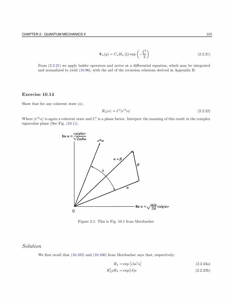
CHAPTER 2: QUANTUM MECHANICS II 105
Ψn(q) = CnHn (ξ) exp
(−ξ
2
2
)(2.2.21)
From (2.2.21) we apply ladder operators and arrive at a differential equation, which may be integratedand normalized to yield (10.96), with the aid of the recursion relations derived in Appendix B.
Exercise 10.14
Show that for any coherent state |α〉,
Rλ|α〉 = C ′|eiλα〉 (2.2.22)
Where |eiλα〉 is again a coherent state and C ′ is a phase factor. Interpret the meaning of this result in the complexeigenvalue plane (See Fig. (10.1)).
Figure 2.1: This is Fig. 10.1 from Merzbacher
Solution
We first recall that (10.105) and (10.106) from Merzbacher says that, respectively:
Rλ =exp[iλa†a
](2.2.23a)
R†λaRλ =exp[iλ]a (2.2.23b)
W. Erbsen HOMEWORK #2
Since Rλ is unitary, we can manipulate (2.2.23b) as:
Rλ
[R†
λaRλ = exp [iλ] a]−→ aRλ =Rλ exp [iλ] a (2.2.24)
Multiplying both sides of (2.2.24) by |α〉 from the right,
aRλ|α〉 = exp [iλ]Rλa|α〉 (2.2.25)
Recalling from (10.97) that a|α〉 = α|α〉, (2.2.25) becomes
aRλ|α〉 = exp [iλ]Rλα|α〉 −→ aRλ|α〉 = α exp [iλ]Rλ|α〉 (2.2.26)
From (2.2.26), we can definitively say that Rλ|α〉 is an eigenvector of a with eigenvalue α exp [iλ].Therefore, Rλ|α〉 creates another coherent state |exp [iλ]α〉 that is offset by some phase factor, whichMerzbacher denotes as C ′. Therefore, we can say that:
Rλ|α〉 = C ′|eiλα〉
It appears as though the unitary operator Rλ is appropriately denoted - it seems to rotate some initialcoherent state |α〉 by some angle λ within the complex plane (See Figure 10.1 above).
Exercise 10.20
For a coherent state |α〉, evaluate the expectation value of the number operator a†a, its square and its vari-ance, using the commutation relation from (10.72). Check the results by computing the expectation values of n,
n2, and (∆n)2
directly from the Poisson distribution, (10.110).
Solution
The commutation relation is [a, a†] = aa† − a†a = 1. We also know that
a|α〉 = α|α〉 (2.2.27)
Where |α〉 is the coherent state. First let’s find the expectation value of N :
〈N〉 =〈α|N |α〉=〈α|a†a|α〉=(〈α|a†
)(a|α〉)
=α∗α
=|α|2 (2.2.28)
And similarly, we now find the expectation value of N2:
〈N2〉 =〈α|(a†a)2|α〉
CHAPTER 2: QUANTUM MECHANICS II 107
=〈α|a†aa†a|α〉=〈α|a†(aa†)a|α〉=〈α|a†(a†a+ 1)a|α〉=〈α|a†a†aa|α〉+ 〈α|a†a|α〉=〈α|a†2a2|α〉+ |α|2
=α∗2α2 + |α|2
=|α|4 + |α|2 (2.2.29)
Where I used the commutation relation and also the result from (2.2.28). Now to find the variance weinsert (2.2.28) and (2.2.29) into the typical equation:
∆N2 =〈N2〉 − 〈N〉2
=|α|4 + |α|2 − (|α|2)2
=|α|4 + |α|2 − |α|4
=|α|2 (2.2.30)
The results (2.2.28), (2.2.29) and (2.2.30) constitute the answer to the first part of the question. Nowwe are asked to find the same quantities using the Poisson distribution:
Pn(α) = e−|α|2 |α|2n
n!(2.2.31)
And recall that if we expand the coherent state |α〉 in terms of the number operator eigenstates |n〉 weget:
|α〉 =
∞∑
n=0
|n〉e−|α|2/2 αn
√n!
(2.2.32)
Which is (10.109) on pg. 227 of Merzbacher. We can then say that
〈α| =
∞∑
n=0
〈n|e−|α|2/2 α∗n
√n!
(2.2.33)
Then to find the expectation value of the number operator, we sandwich n between (2.2.33) and (2.2.32),respectively:
〈n〉 =〈α|n|α〉=(〈α|) (n|α〉)
=
( ∞∑
n=0
〈n|e−|α|2/2 α∗n
√n!
)( ∞∑
n=0
n|n〉e−|α|2/2 αn
√n!
)
=e−|α|2∞∑
n=0
nα∗nαn
n!〈n|n〉
=e−|α|2∞∑
n=0
n|α|2n
n!(2.2.34)
W. Erbsen HOMEWORK #2
Now we must jiggle this equation around a little to arrive at the solution. First it is important to noticethat
n
n!=
n
1 · 2 · 3 · ... · n − 1 · n=
1
1 · 2 · 3 · ... · n − 1
=1
(n− 1)!(2.2.35)
Also recall the power series expansion of ex2
ex2
=
∞∑
k=0
x2k
k!(2.2.36)
Applying (2.2.35) and (2.2.36) to 〈n〉 in (2.2.34),
〈n〉 =e−|α|2∞∑
n=0
n|α|2n
n!
=|α|2e−|α|2∞∑
n=0
|α|2(n−1)
(n− 1)!(2.2.37)
Letting k = n− 1,
〈n〉 =|α|2e−|α|2∞∑
k=0
|α|2k
k!
=|α|2e−|α|2e|α|2
=|α|2 (2.2.38)
Which agrees with (2.2.28). Now let’s do the same thing for 〈n2〉. Using the results from (2.2.34):
〈n2〉 =
∞∑
n=0
n2 |α|2n
n!
=
∞∑
n=0
n|α|2n
(n− 1)!
(2.2.39)
Now go ahead and shift the index, making this easier to solve. Let n = k + 1 → k = n− 1:
〈n2〉 =e−|α|2∞∑
k=0
(k + 1)|α|2(k+1)
k!
=e−|α|2∞∑
k=0
k|α|2(k+1)
k!+ e−|α|2
∞∑
k=0
|α|2(k+1)
k!
=e−|α|2 |α|4∞∑
k=0
|α|2(k−1)
(k − 1)!+ e−|α|2 |α|2
∞∑
k=0
|α|2k
k!
CHAPTER 2: QUANTUM MECHANICS II 109
=e−|α|2 |α|4e|α|2 + e−|α|2|α|2e|α|2
=|α|4 + |α|2 (2.2.40)
Which agrees with (2.2.29).
Problem 10.2
Assuming a particle to be in one of the stationary states of an infinitely high one-dimensional box, calculatethe uncertainties in position and momentum, and show that they agree with the Heisenberg uncertainty relation.Also show that in the limit of very large quantum numbers, the uncertainty in x equals the root-mean-squaredeviation of the position of a particle moving in the enclosure classically with the same energy.
Solution
Assuming that our infinite potential well has a length denoted by a, the (normalized) eigenfunctions aregiven by
ψn(x) =
√2
asin(nπx
a
)(2.2.41)
To find the uncertainties in both position and momentum in the quantum regime, we must calculate thestandard deviation of each quantity
∆x =√
〈x2〉 − 〈x〉2 , ∆p =√
〈p2〉 − 〈p〉2 (10.2.2a,b)
So, our task is to calculate 〈x〉, 〈x2〉, 〈p〉, and 〈p2〉. In these calculations I will be using two integrationtechniques: integration by parts and trig substitutions. In particular I will use sin2(ax) = 1/2(1 −cos(2ax)) and also
∫sin(ax) cos(ax) dx = 1/2a sin2(ax). Let’s go ahead and calculate 〈x〉 first:
〈x〉 =
∫ a
0
ψ∗n(x)xψn(x) dx
=2
a
∫ a
0
x sin2(nπx
a
)dx
=2
a
∫ a
0
x
[1
2− 1
2cos
(2nπx
a
)]dx
=1
a
[∫ a
0
x dx−∫ a
0
x cos
(2nπx
a
)dx
]
=1
a
[a2
2−∫ a
0
x cos
(2nπx
a
)dx
]
=1
a
[a2
2−([
xa
2nπsin
(2nπx
a
)∣∣∣∣a
0
− a
2nπ
∫ a
0
sin
(2nπx
a
)dx
)]
=1
a
[a2
2−(a2
2nπsin(2nπ) +
( a
2nπ
)2[cos
(2nπx
a
)∣∣∣∣a
0
)]
W. Erbsen HOMEWORK #2
=1
a
[a2
2−(( a
2nπ
)2
(cos(2nπ) − cos(0))
)]
=1
a
(a2
2
)
=a
2(2.2.3)
This is not surprising, and in fact this fact coincides with the classical result, which I discuss at the endof this problem. Now let’s do the same for 〈x2〉:
〈x2〉 =
∫ a
0
ψ∗n(x)x2ψn(x) dx
=2
a
∫ a
0
x2 sin2(nπx
a
)dx
=2
a
∫ a
0
x2
[1
2− 1
2cos
(2nπx
a
)]dx
=2
a
[∫ a
0
x2
2dx−
∫ a
0
x2
2cos
(2nπx
a
)dx
]
=2
a
[a3
6− 1
2
∫ a
0
x2 cos
(2nπx
a
)dx
]
=2
a
[a3
6− 1
2
[[ax2
2nπsin
(2nπx
a
)∣∣∣∣a
0
− a
nπ
∫ a
0
x sin
(2nπx
a
)dx
]]
=2
a
[a3
6+
a
2nπ
[∫ a
0
x sin
(2nπx
a
)dx
]]
=2
a
[a3
6+
a
2nπ
([ax
2nπcos
(2nπx
a
)∣∣∣∣a
0
+a
2nπ
∫ a
0
cos
(2nπx
a
)dx
)]
=2
a
[a3
6+
a
2nπ
(a2
2nπ
)]
=2
a
[a3
6− a3
4n2π2
]
=a2
3− a2
2n2π2(2.2.4)
This is not immediately intuitive, but it is possible to draw understanding from it when comparing it tothe classical analogue. Now let’s head off to calculate the momentum expectation value 〈p〉:
〈p〉 =
∫ a
0
ψ∗n
(~
i
d
dx
)ψn(x) dx
=2
a
~
i
∫ a
0
sin(nπx
a
) d
dxsin(nπx
a
)dx
=2
a
~
i
nπ
a
∫ a
0
sin(nπx
a
)cos(nπx
a
)dx
=2
a
~
i
nπ
a
[1
2asin2
(nπxa
)∣∣∣∣a
0
=0 (2.2.5)
CHAPTER 2: QUANTUM MECHANICS II 111
We could have guessed this result since ψn(x) is real. On the other hand, 〈p2〉 is not zero:
〈p2〉 =
∫ a
0
ψ∗n
(~
i
d
dx
)2
ψn(x) dx
=2
a
(~
i
)2 ∫ a
0
sin(nπx
a
)( d
dx
)2
sin(nπx
a
)dx
=2
a
(~
i
)2nπ
a
∫ a
0
sin(nπx
a
)( d
dx
)cos(nπx
a
)dx
=2
a(~)2
(nπa
)2∫ a
0
sin2(nπx
a
)dx
=2
a(~)2
(nπa
)2∫ a
0
(1
2− 1
2cos
(2nπx
a
))dx
=2
a(~)2
(nπa
)2[1
2
∫ a
0
dx− 1
2
∫ a
0
cos
(2nπx
a
)dx
]
=2
a(~)2
(nπa
)2 [a2
]
=~2n2π2
a2(2.2.6)
So now we can go ahead and compute the uncertainties in position and momentum by substituting (2.2.3)and (2.2.4) into (10.2.2a) and also (2.2.5) and (2.2.6) into (10.2.2b), respectively. Starting first with theposition,
∆x =√
〈x2〉 − 〈x〉2
=
√(a2
3− a2
2n2π2
)−(a
2
)2
=
√a2
3− a2
2n2π2− a2
42
−→ ∆x =
√a2
12− a2
2n2π2(2.2.7)
And now the momentum,
∆p =√〈p2〉 − 〈p〉2 ⇒
√(~2n2π2
a2
)− 0 −→ ∆p =
~nπ
a(2.2.8)
To check to see if these results are consistent with the Heisenberg uncertainty relation, multiply (2.2.7)and (2.2.8):
∆x∆p =
(a2
12− a2
2n2π2
)1/2 (~2n2π2
a2
) 1/2
=
(~2n2π2
12− ~2
2
)1/2
=~
2
(n2π2
3− 2
)1/2
(2.2.9)
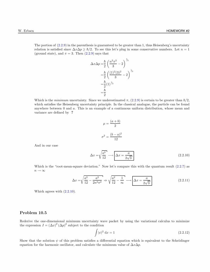
W. Erbsen HOMEWORK #2
The portion of (2.2.9) in the parenthesis is guaranteed to be greater than 1, thus Heisenberg’s uncertaintyrelation is satisfied since ∆x∆p ≥ ~/2. To see this let’s plug in some conservative numbers. Let n = 1(ground state), and π = 3. Then (2.2.9) says that
∆x∆p =~
2
(n2π2
3− 2
) 1/2
=~
2
((1)2(3)2
3− 2
) 1/2
=~
2(1)
1/2
=~
2
Which is the minimum uncertainty. Since we underestimated π, (2.2.9) is certain to be greater than ~/2,which satisfies the Heisenberg uncertainty principle. In the classical analogue, the particle can be foundanywhere between 0 and a. This is an example of a continuous uniform distribution, whose mean andvariance are defined by ?
µ =(a + b)
2
σ2 =(b − a)2
12
And in our case
∆x =
√a2
12−→ ∆x =
a
2√
3(2.2.10)
Which is the “root-mean-square deviation.” Now let’s compare this with the quantum result (2.2.7) asn → ∞
∆x =
√a2
12− a2
2n2π2⇒√a2
12− 1
∞ −→ ∆x =a
2√
3(2.2.11)
Which agrees with (2.2.10).
Problem 10.5
Rederive the one-dimensional minimum uncertainty wave packet by using the variational calculus to minimizethe expression I = (∆x)
2(∆p)
2subject to the condition∫
|ψ|2 dx = 1 (2.2.12)
Show that the solution ψ of this problem satisfies a differential equation which is equivalent to the Schrodingerequation for the harmonic oscillator, and calculate the minimum value of ∆x∆p.
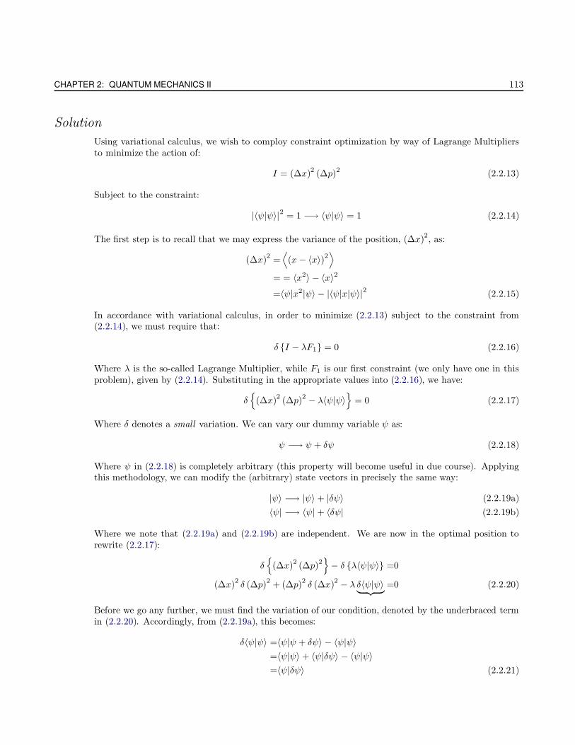
CHAPTER 2: QUANTUM MECHANICS II 113
Solution
Using variational calculus, we wish to comploy constraint optimization by way of Lagrange Multipliersto minimize the action of:
I = (∆x)2 (∆p)2 (2.2.13)
Subject to the constraint:
|〈ψ|ψ〉|2 = 1 −→ 〈ψ|ψ〉 = 1 (2.2.14)
The first step is to recall that we may express the variance of the position, (∆x)2, as:
(∆x)2
=⟨(x− 〈x〉)2
⟩
= = 〈x2〉 − 〈x〉2
=〈ψ|x2|ψ〉 − |〈ψ|x|ψ〉|2 (2.2.15)
In accordance with variational calculus, in order to minimize (2.2.13) subject to the constraint from(2.2.14), we must require that:
δ I − λF1 = 0 (2.2.16)
Where λ is the so-called Lagrange Multiplier, while F1 is our first constraint (we only have one in thisproblem), given by (2.2.14). Substituting in the appropriate values into (2.2.16), we have:
δ
(∆x)2(∆p)
2 − λ〈ψ|ψ〉
= 0 (2.2.17)
Where δ denotes a small variation. We can vary our dummy variable ψ as:
ψ −→ ψ + δψ (2.2.18)
Where ψ in (2.2.18) is completely arbitrary (this property will become useful in due course). Applyingthis methodology, we can modify the (arbitrary) state vectors in precisely the same way:
|ψ〉 −→ |ψ〉 + |δψ〉 (2.2.19a)
〈ψ| −→ 〈ψ| + 〈δψ| (2.2.19b)
Where we note that (2.2.19a) and (2.2.19b) are independent. We are now in the optimal position torewrite (2.2.17):
δ
(∆x)2(∆p)
2− δ λ〈ψ|ψ〉 =0
(∆x)2δ (∆p)
2+ (∆p)
2δ (∆x)
2 − λ δ〈ψ|ψ〉︸ ︷︷ ︸=0 (2.2.20)
Before we go any further, we must find the variation of our condition, denoted by the underbraced termin (2.2.20). Accordingly, from (2.2.19a), this becomes:
δ〈ψ|ψ〉 =〈ψ|ψ + δψ〉 − 〈ψ|ψ〉=〈ψ|ψ〉 + 〈ψ|δψ〉 − 〈ψ|ψ〉=〈ψ|δψ〉 (2.2.21)
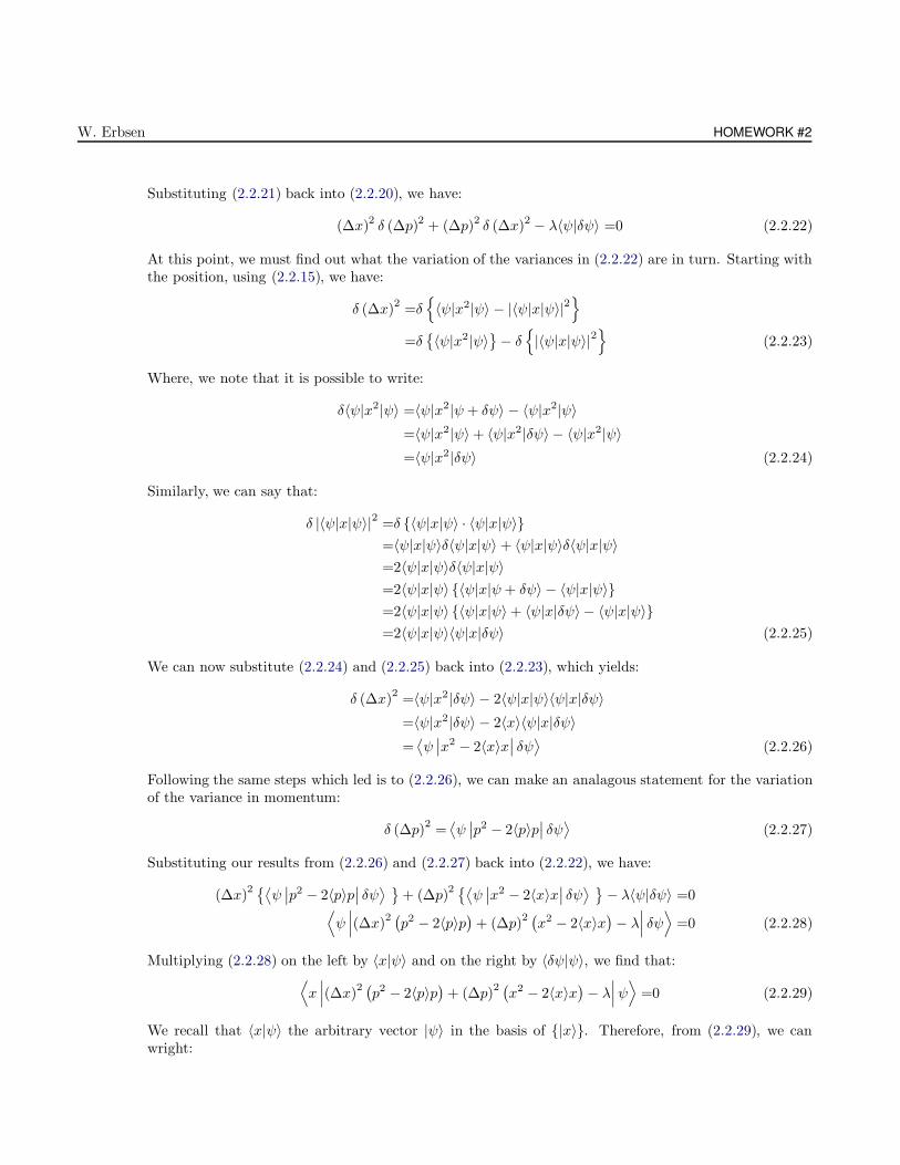
W. Erbsen HOMEWORK #2
Substituting (2.2.21) back into (2.2.20), we have:
(∆x)2 δ (∆p)2 + (∆p)2 δ (∆x)2 − λ〈ψ|δψ〉 =0 (2.2.22)
At this point, we must find out what the variation of the variances in (2.2.22) are in turn. Starting withthe position, using (2.2.15), we have:
δ (∆x)2
=δ〈ψ|x2|ψ〉 − |〈ψ|x|ψ〉|2
=δ〈ψ|x2|ψ〉
− δ
|〈ψ|x|ψ〉|2
(2.2.23)
Where, we note that it is possible to write:
δ〈ψ|x2|ψ〉 =〈ψ|x2|ψ + δψ〉 − 〈ψ|x2|ψ〉=〈ψ|x2|ψ〉 + 〈ψ|x2|δψ〉 − 〈ψ|x2|ψ〉=〈ψ|x2|δψ〉 (2.2.24)
Similarly, we can say that:
δ |〈ψ|x|ψ〉|2 =δ 〈ψ|x|ψ〉 · 〈ψ|x|ψ〉=〈ψ|x|ψ〉δ〈ψ|x|ψ〉 + 〈ψ|x|ψ〉δ〈ψ|x|ψ〉=2〈ψ|x|ψ〉δ〈ψ|x|ψ〉=2〈ψ|x|ψ〉 〈ψ|x|ψ + δψ〉 − 〈ψ|x|ψ〉=2〈ψ|x|ψ〉 〈ψ|x|ψ〉 + 〈ψ|x|δψ〉 − 〈ψ|x|ψ〉=2〈ψ|x|ψ〉〈ψ|x|δψ〉 (2.2.25)
We can now substitute (2.2.24) and (2.2.25) back into (2.2.23), which yields:
δ (∆x)2
=〈ψ|x2|δψ〉 − 2〈ψ|x|ψ〉〈ψ|x|δψ〉=〈ψ|x2|δψ〉 − 2〈x〉〈ψ|x|δψ〉=⟨ψ∣∣x2 − 2〈x〉x
∣∣ δψ⟩
(2.2.26)
Following the same steps which led is to (2.2.26), we can make an analagous statement for the variationof the variance in momentum:
δ (∆p)2
=⟨ψ∣∣p2 − 2〈p〉p
∣∣ δψ⟩
(2.2.27)
Substituting our results from (2.2.26) and (2.2.27) back into (2.2.22), we have:
(∆x)2 ⟨
ψ∣∣p2 − 2〈p〉p
∣∣ δψ⟩
+ (∆p)2 ⟨
ψ∣∣x2 − 2〈x〉x
∣∣ δψ⟩
− λ〈ψ|δψ〉 =0⟨ψ∣∣∣(∆x)2
(p2 − 2〈p〉p
)+ (∆p)
2 (x2 − 2〈x〉x
)− λ
∣∣∣ δψ⟩
=0 (2.2.28)
Multiplying (2.2.28) on the left by 〈x|ψ〉 and on the right by 〈δψ|ψ〉, we find that:⟨x∣∣∣(∆x)2
(p2 − 2〈p〉p
)+ (∆p)
2 (x2 − 2〈x〉x
)− λ
∣∣∣ψ⟩
=0 (2.2.29)
We recall that 〈x|ψ〉 the arbitrary vector |ψ〉 in the basis of |x〉. Therefore, from (2.2.29), we canwright:
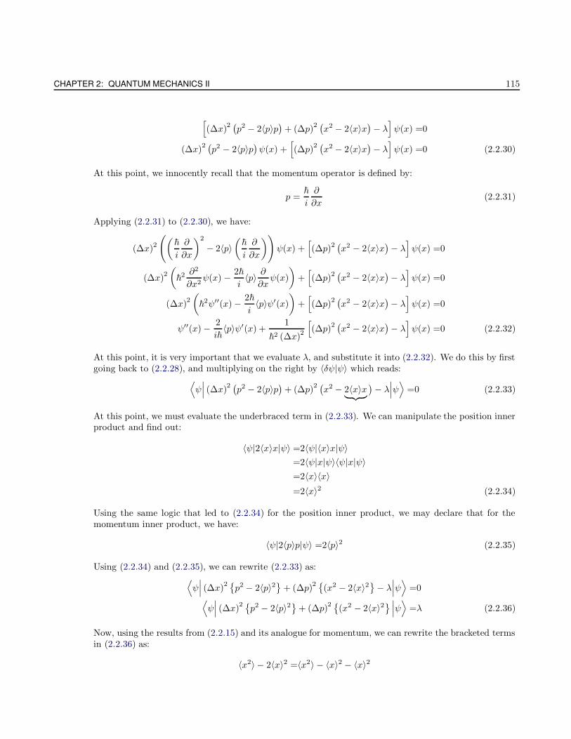
CHAPTER 2: QUANTUM MECHANICS II 115
[(∆x)
2 (p2 − 2〈p〉p
)+ (∆p)
2 (x2 − 2〈x〉x
)− λ]ψ(x) =0
(∆x)2 (p2 − 2〈p〉p
)ψ(x) +
[(∆p)
2 (x2 − 2〈x〉x
)− λ]ψ(x) =0 (2.2.30)
At this point, we innocently recall that the momentum operator is defined by:
p =~
i
∂
∂x(2.2.31)
Applying (2.2.31) to (2.2.30), we have:
(∆x)2((
~
i
∂
∂x
)2
− 2〈p〉(
~
i
∂
∂x
))ψ(x) +
[(∆p)2
(x2 − 2〈x〉x
)− λ
]ψ(x) =0
(∆x)2
(~2 ∂
2
∂x2ψ(x) − 2~
i〈p〉 ∂
∂xψ(x)
)+[(∆p)
2 (x2 − 2〈x〉x
)− λ
]ψ(x) =0
(∆x)2
(~2ψ′′(x) − 2~
i〈p〉ψ′(x)
)+[(∆p)
2 (x2 − 2〈x〉x
)− λ
]ψ(x) =0
ψ′′(x) − 2
i~〈p〉ψ′(x) +
1
~2 (∆x)2
[(∆p)
2 (x2 − 2〈x〉x
)− λ
]ψ(x) =0 (2.2.32)
At this point, it is very important that we evaluate λ, and substitute it into (2.2.32). We do this by firstgoing back to (2.2.28), and multiplying on the right by 〈δψ|ψ〉 which reads:
⟨ψ∣∣∣ (∆x)2
(p2 − 2〈p〉p
)+ (∆p)
2 (x2 − 2〈x〉x︸ ︷︷ ︸
)− λ
∣∣∣ψ⟩
=0 (2.2.33)
At this point, we must evaluate the underbraced term in (2.2.33). We can manipulate the position innerproduct and find out:
〈ψ|2〈x〉x|ψ〉 =2〈ψ|〈x〉x|ψ〉=2〈ψ|x|ψ〉〈ψ|x|ψ〉=2〈x〉〈x〉=2〈x〉2 (2.2.34)
Using the same logic that led to (2.2.34) for the position inner product, we may declare that for themomentum inner product, we have:
〈ψ|2〈p〉p|ψ〉 =2〈p〉2 (2.2.35)
Using (2.2.34) and (2.2.35), we can rewrite (2.2.33) as:⟨ψ∣∣∣ (∆x)2
p2 − 2〈p〉2
+ (∆p)
2 (x2 − 2〈x〉2
− λ
∣∣∣ψ⟩
=0⟨ψ∣∣∣ (∆x)2
p2 − 2〈p〉2
+ (∆p)
2 (x2 − 2〈x〉2
∣∣∣ψ⟩
=λ (2.2.36)
Now, using the results from (2.2.15) and its analogue for momentum, we can rewrite the bracketed termsin (2.2.36) as:
〈x2〉 − 2〈x〉2 =〈x2〉 − 〈x〉2 − 〈x〉2
W. Erbsen HOMEWORK #2
=(∆x)2 − 〈x〉2 (2.2.37)
And similarly, for the momentum:
〈p2〉 − 2〈p〉2 =(∆p)2 − 〈p〉2 (2.2.38)
Applying (2.2.37) and (2.2.38) to (2.2.36), we have:
(∆x)2
(∆p)2 − 〈p〉2
+ (∆p)
2
(∆x)2 − 〈x〉2
= λ
(∆x)2(∆p)
2 − (∆x)2 〈p〉2 + (∆p)
2(∆x)
2 − (∆p)2 〈x〉2 = λ
2 (∆x)2(∆p)
2 − (∆x)2 〈p〉2 − (∆p)
2 〈x〉2 = λ (2.2.39)
Now, substituting (2.2.39) back into (2.2.32)
ψ′′(x) − 2
i~〈p〉ψ′(x)
+1
~2 (∆x)2
[(∆p)
2 (x2 − 2〈x〉x
)−[2 (∆x)
2(∆p)
2 − (∆x)2 〈p〉2 − (∆p)
2 〈x〉2]]ψ(x) = 0
ψ′′(x) − 2
i~〈p〉ψ′(x)
+1
~2 (∆x)2
[(∆p)
2 (x2 − 2〈x〉x
)− 2 (∆x)
2(∆p)
2+ (∆x)
2 〈p〉2 + (∆p)2 〈x〉2
]ψ(x) = 0
ψ′′(x) − 2
i~〈p〉ψ′(x)
+1
~2 (∆x)2
[(∆p)
2 (x2 − 2〈x〉x+ 〈x〉2
)− 2 (∆x)
2(∆p)
2+ (∆x)
2 〈p〉2]ψ(x) = 0
ψ′′(x) − 2
i~〈p〉ψ′(x) +
1
~2 (∆x)2
[(∆p)
2(x− 〈x〉)2 − 2 (∆x)
2(∆p)
2+ (∆x)
2 〈p〉2]ψ(x) = 0
ψ′′(x) − 2
i~〈p〉ψ′(x) +
1
~2
[(∆p)
2
(∆x)2 (x− 〈x〉)2 − 2 (∆p)
2+ 〈p〉2
]ψ(x) = 0 (2.2.40)
At this point, we suppose that the wave function ψ(x) can be expressed as:
ψ(x) = exp
[i〈p〉x
~
]φ(x) (2.2.41)
Whose first and second derivative are
ψ′(x) =i〈p〉~
exp
[i〈p〉x
~
]φ(x) + exp
[i〈p〉x
~
]φ′(x) (2.2.42a)
ψ′′(x) = − 〈p〉2~2
exp
[i〈p〉x
~
]φ(x) +
i〈p〉~
exp
[i〈p〉x
~
]φ′(x) +
i〈p〉~
exp
[i〈p〉x
~
]φ′(x) + exp
[i〈p〉x
~
]φ′′(x)
(2.2.42b)
CHAPTER 2: QUANTUM MECHANICS II 117
We now wish to substitute (2.2.41), (2.2.42a), and (2.2.42b) back into (2.2.40). We first recognize thatthe exponential terms cancel, and so we are left with:
[−〈p〉2
~2φ+
i〈p〉~φ′ +
i〈p〉~φ′ + φ′′
]− 2
i~〈p〉[i〈p〉~φ+ φ′
]+
1
~2
[(∆p)
2
(∆x)2 (x− 〈x〉)2 − 2 (∆p)
2+ 〈p〉2
]φ = 0
−〈p〉2~2
φ+2i〈p〉
~φ′ + φ′′ − 2〈p〉2
~2φ− 2〈p〉
i~φ′ +
1
~2
[(∆p)
2
(∆x)2 (x− 〈x〉)2 − 2 (∆p)
2+ 〈p〉2
]φ = 0
φ′′ +1
~2
[(∆p)
2
(∆x)2 (x− 〈x〉)2 − 2 (∆p)
2+ 〈p〉2 − 〈p〉2 − 2〈p〉2
]φ = 0
φ′′ +1
~2
[(∆p)
2
(∆x)2 (x− 〈x〉)2 − 2
((∆p)
2+ 〈p〉2
)]φ = 0
φ′′ +1
~2
[(∆p)
2
(∆x)2 (x− 〈x〉)2 − 2〈p2〉
]φ = 0
(2.2.43)
At this point, we let (∆p)/ (∆x) → mω (the reasons why we chose our constants as m and ω will becomeclear momentarily. Accordingly, (2.2.43) becomes
~2φ′′ +[m2ω2 (x− 〈x〉)2 − 2〈p2〉
]φ =0 (2.2.44)
We can divide both sides of (2.2.44) by 2m, which yields:
~2
2mφ′′(x) +
mω2
2(x− 〈x〉)2 φ(x) =
〈p2〉m
φ(x) (2.2.45)
We can see that (2.2.45) looks an awful lot like the time-independent Schrodinger Equation with the 1-DHarmonic Oscillator Hamiltonian. We can manipulate it slightly more,
[p2
2m+mω2
2(x− 〈x〉)2
]φ(x) =
〈p2〉m
φ(x) (2.2.46)
We now recall that for the 1-D Harmonic Oscillator, from (A.9) and (A.12), we recall that:
〈x〉 = 0, 〈p2〉 =~mω
2(2n+ 1)
Applying this to (2.2.46), we have:
[p2
2m+mω2
2x2
]φ(x) = ~ω
(n+ 1/2
)φ(x) (2.2.47)
Letting En = ~ω(n+ 1/2
)for obvious reasons, we should now be sufficiently convinced that the solution
of this problem is fully equivalent to the Schrodinger equation for the 1-D Harmonic Oscillator. Lettingφ(x) → ψn(x), (2.2.47) becomes:
[p2
2m+mω2
2x2
]ψn(x) = Enψn(x)
W. Erbsen HOMEWORK #2
The solution for this differential equation is given by (5.49) in Merzbacher as:
ψn(x) = 2−n/2 (n!)−1/2
(mω~π
)1/4exp
(−mω
2~x2)Hn
(√mω
~x
)(2.2.48)
We can find the 1-D minimum uncertainty wave packet by other means, though. Following Merzbacher’swork on pgs. 218-219, starting with (10.55), we have:
∆A2∆B2 ≥ |(Ψ, (A− 〈A〉)(B − 〈B〉)Ψ)|2 (2.2.49)
Where in our case A ⇒ x and B ⇒ p. Remember that we are looking for the minimum uncertaintystate, so to find the ground state wave function with minimum uncertainty we would take the “≥” in(2.2.49) to be a “=.” This holds if and only if
(p− 〈p〉)Ψ = λ(x − 〈x〉)Ψ (2.2.50)
Which is analogous to (10.56) in Merzbacher. With a little manipulation we can see that (2.2.50) is infact a differential equation
(p − 〈p〉)Ψ − λ(x − 〈x〉)Ψ =0(
~
i
∂
∂x− 〈p〉
)Ψ − λ(x − 〈x〉)Ψ =0 (2.2.51)
Where Merzbacher has provided us with the derivation and value of λ = i〈C〉/2∆A2, where in our case〈C〉 = ~. Substituting this into (2.2.51):
(~
i
∂
∂x− 〈p〉
)Ψ − i~
2∆x2λ(x− 〈x〉)Ψ =0
dψ
dx+
(−i〈p〉~
+(x− 〈x〉)
2∆x2
)Ψ =0 (2.2.52)
Which is a separable differential equation, and the solution is found by
1
ΨdΨ =
(i〈p〉~
− (x− 〈x〉)2∆x2
)dx
log (Ψ) =
∫−(x − 〈x〉)
2∆x2dx+
∫i〈p〉~
dx
= − (x− 〈x〉)24∆x2
+i〈p〉x
~+ C
Ψ = C exp
[−(x − 〈x〉)2
4∆x2+i〈p〉x
~
](2.2.53)
And normalizing,
∫ ∞
−∞|Ψ|2 dx =1
∫ ∞
−∞
∣∣∣∣C exp
[−(x− 〈x〉)2
4∆x2+i〈p〉x
~
]∣∣∣∣2
dx =1
CHAPTER 2: QUANTUM MECHANICS II 119
C2
∫ ∞
−∞exp
[−(x− 〈x〉)2
2∆x2
]=1
C2(2π∆x2
) 12 =1
C =(2π∆x2
)−1/4(2.2.54)
So our ground state wave function, (2.2.53), combined with the appropriate normalization constant,(2.2.54), is given by
Ψ =(2π∆x2
)−1/4exp
[−(x− 〈x〉)2
4∆x2+i〈p〉x
~
](2.2.55)
Which is identical to (10.66). An important note would be that (2.2.55) minimizes the uncertainty, whichwill come in handy later on when we reach problems addressing with coherent and squeezed states.
Problem 10.6
The Hamiltonian representing an oscillating LC circuit can be expressed as
H =Q2
2C+
Φ2
2L(2.2.56)
Establish that Hamilton’s equations are the correct dynamical equations for this system, and show that the chargeQ and the magnetic flux Φ can be regarded as canonically conjugate variables q, p (or the dual pair p, −q).Work out the Heisenberg relation for the product of the uncertainties in the current I and the voltage V . If amesoscopic LC circuit has an effective inductance of L = 1 µH and an effective capacitance C = 1 pF, how lowmust the temperature of the device be before quantum fluctuations become comparable to thermal energies? Arethe corresponding current-voltage tolerances in the realm of observability?
Solution
Hamilton’s equations are given by:
qi =∂H
∂pi(2.2.57a)
−pi =∂H
∂qi(2.2.57b)
Where (2.2.57a) and (2.2.57b) are from (8.18) from Goldstein on pg. 337 ?. We note that in our case the“position” is the magnetic flux, and the “momentum” is the charge. Accordingly, (2.2.57a) and (2.2.57b)become
Φ =∂H
∂Q(2.2.58a)
−Q =∂H
∂Φ(2.2.58b)
W. Erbsen HOMEWORK #2
Substituting (2.2.56) into (2.2.58a) and (2.2.59b),
Φ =∂
∂Q
[Q2
2C+
Φ2
2L
]⇒ Φ =
Q
C(2.2.59a)
−Q =∂
∂Φ
[Q2
2C+
Φ2
2L
]⇒ Q = −Φ
L(2.2.59b)
The best way to proceed with this problem is to mimic the same procedure for the Quantum HarmonicOscillator. We begin by drawing a direct analogue between the position and momentum operatorswith the magnetic flux and charge operators, respectively. Starting with the position → magnetic fluxrelationship, we recall from (A.2a) that
q =
√~
2mω
(a† + a
)(2.2.60)
In the case where we let q → Φ, we must also let ω → (LC)1/2 , and m → C. Accordingly, (2.2.60)
becomes:
Φ =
√~
2
(L
C
) 1/4 (c† + c
)(2.2.61)
Where c and c† are to be defined momentarily. We now draw correlation between the momentum operatorfrom (A.2b) to the charge operator:
Q = i
√~
2
(C
L
) 1/4 (c† − c
)(2.2.62)
It is easy to see from (A.9) and (A.11) that 〈Φ〉 = 〈Q〉 = 0. From (A.10), we have:
〈Φ2〉 = ~
√L
C
(n+ 1/2
)(2.2.63)
While from (A.12) we can see that:
〈Q2〉 = ~
√C
L
(n+ 1/2
)(2.2.64)
From (2.2.63) and (2.2.64), we can now calculate the variance of the magnetic flux and charge:
(∆Φ)2
=〈Φ2〉 − 〈Φ〉2 ⇒ ~
√L
C
(n+ 1/2
)(2.2.65a)
(∆Q)2
=〈Q2〉 − 〈Q〉2 ⇒ ~
√C
L
(n + 1/2
)(2.2.65b)
We are asked to find the product of the uncertainties in the current I and the voltage V , however (2.2.65a)and (2.2.65b) are in terms of Φ and Q, respectively. We can use (2.2.60) and (2.2.59b) to connect thetwo respective quantities:
Φ ⇒V =Q
C−→ Q = CV (2.2.66a)
−Q⇒I =Φ
L−→ Φ = LI (2.2.66b)
CHAPTER 2: QUANTUM MECHANICS II 121
So, using (2.2.66a) and (2.2.66b), then (2.2.65a) and (2.2.65b) become
(∆I)2
=~
√1
LC
(n+ 1/2
)(2.2.67a)
(∆V )2
=~
√1
LC
(n+ 1/2
)(2.2.67b)
We now multiply (2.2.67a) and (2.2.67b), which yields
∆I∆V =~√LC
(n+ 1/2
)
Given the provided parameters, we are now in a position to find the temperature at which quantumfluctuations become apparent. We achieve this by setting the zero-point energy equal to the averagethermal energy, and solving for T :
~
2
1√LC
−→ T =~
2kB
1√LC
=1.055× 10⁻³⁴ J · s
2 (1.381× 10⁻²³ J · s−1)
1√(1 × 10⁻⁶ H) (1 × 10⁻¹² F)
−→ T ≈ 3.82× 10⁻³ K (2.2.68)
Problem 10.7
If a coherent state |α〉 (eigenstate of a) of an oscillator is transformed into a squeezed state by the unitaryoperator
U = exp
[ζ
2(a2 − a†2)
](2.2.69)
calculate the value of ζ that will reduce the width of the Hermitian observable (a + a†)/√
2 to 1 percent of itsoriginal coherent-state value. What happens to the width of the conjugate observable (a− a†)/
√2 i in this trans-
formation?
Solution
We know that |α〉 is an eigenstate of a and satisfies a|α〉 = α|α〉. What we want to do is go from ourcoherent state |α〉 to a squeezed state |α, ζ〉. We arrive at the squeezed state by applying a unitaryoperator, (2.2.69), to our coherent state: U|α〉 = |α, ζ〉. To do this, we first find the squeezed stateoperator, b, which we define as:
b =UaU†
U†b =aU†
U†BU =a (2.2.70)

W. Erbsen HOMEWORK #2
So we can say:
〈α|a|α〉 =〈α|U†bU|α〉=〈α, ζ|b|α, ζ〉 (2.2.71)
The easiest way to find b would be to utilize some identities made available by Merzbacher on pgs. 39-40.He says that if
f(λ) = eλABe−λA
Then we can write
f(λ) = B cosh λ√β +
[A,B]√β
sinhλ√β (2.2.72)
Which we can use only if β is constant, and the operators A and B satisfy [A, [A,B]] = βB. In our case,f(λ) → b(ζ), and A = (a2 − a†2) and B = a. To find out if we can use (2.2.72):
[A,B] =[(a2 − a†2), a]
=[a2, a]− [a†2, a]
= − [a†2, a]
= − a†[a†, a]− [a†, a]a†
= − a†(−1) − (−1)a†
=2a† (2.2.73)
[A, [A,B]] =[(a2 − a†2), 2a†]
=2([a2, a†]− [a†2a†]
)
=2(a[a, a†] + [a, a†]a
)
=4a (2.2.74)
It seems that we can in fact use (2.2.72), since both of our conditions are satisfied with λ = −ζ/2 andβ = 4. We now have,
b(ζ) =a coshλ√β +
[A,B]√β
sinhλ√β
=a cosh−ζ/2√
4 +2a†√
4sinh−ζ/2
√4
=a cosh ζ + a† sinh ζ
=a cosh ζ − a† sinh ζ (2.2.75)
Following Merzbacher’s lead on pgs. 230-231, we define λ = cosh ζ and ν = sinh ζ, where λ here isdifferent than the one used before. We can now rewrite (2.2.75):
b = λa+ νa† (2.2.76)
CHAPTER 2: QUANTUM MECHANICS II 123
And taking the Hermitian conjugate,
b† = λa† + νa (2.2.77)
Since both λ and ν are real. Inverting these two equations
a = λb− νb† (2.2.78)
a† = λb† − νb (2.2.79)
And we can now write
1√2〈α|a|α〉 =
1√2〈α, ζ|b|α, ζ〉
=1√2〈α, ζ|λa+ νa†|α, ζ〉 (2.2.80)
1√2〈α|a†|α〉 =
1√2〈α, ζ|b†|α, ζ〉
=1√2〈α, ζ|λa† + νa|α, ζ〉 (2.2.81)
Now that we have the framework laid down, we can now attack our problem head on and directlyinvestigate the Hermitian conjugate we are to minimize, (a+ a†)/
√2 :
1√2〈α|a+ a†|α〉 =
1√2
[〈α|a|α〉+ 〈α|a†|α〉
]
=1√2
[〈α, ζ|λa+ νa†|α, ζ〉+ 〈α, ζ|λa† + νa|α, ζ〉
]
=1√2〈α, ζ|λa+ νa† + λa† + νa|α, ζ〉
=1√2〈α, ζ|a(λ+ ν) + a†(λ+ ν)|α, ζ〉
=1√2
(λ + ν)〈α, ζ|a+ a†|α, ζ〉
=1√2
(cosh ζ − sinh ζ)〈α, ζ|a+ a†|α, ζ〉
=1√2e−ζ 〈α, ζ|a+ a†|α, ζ〉 (2.2.82)
And we are asked to calculate the value of ζ that “squeezes” (a+ a†)/√
2 to 1% of its original coherentstate value. So take the appropriate fraction, and solve for the squeezing parameter ζ:
1/√
2 e−ζ〈α, ζ|a+ a†|α, ζ〉1/
√2 〈α|a+ a†|α〉(100)
=e−ζ
100(2.2.83)
And finally
eζ = 100 ⇒ ζ = log 100 ≈ 4.60517 . . .
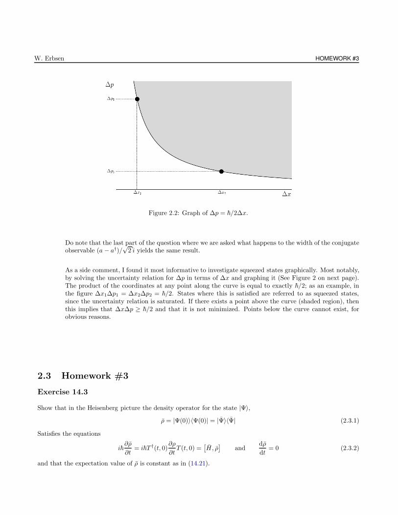
W. Erbsen HOMEWORK #3
Figure 2.2: Graph of ∆p = ~/2∆x.
Do note that the last part of the question where we are asked what happens to the width of the conjugateobservable (a − a†)/
√2 i yields the same result.
As a side comment, I found it most informative to investigate squeezed states graphically. Most notably,by solving the uncertainty relation for ∆p in terms of ∆x and graphing it (See Figure 2 on next page).The product of the coordinates at any point along the curve is equal to exactly ~/2; as an example, inthe figure ∆x1∆p1 = ∆x2∆p2 = ~/2. States where this is satisfied are referred to as squeezed states,since the uncertainty relation is saturated. If there exists a point above the curve (shaded region), thenthis implies that ∆x∆p ≥ ~/2 and that it is not minimized. Points below the curve cannot exist, forobvious reasons.
2.3 Homework #3
Exercise 14.3
Show that in the Heisenberg picture the density operator for the state |Ψ〉,
ρ = |Ψ(0)〉〈Ψ(0)| = |Ψ〉〈Ψ| (2.3.1)
Satisfies the equations
i~∂ρ
∂t= i~T †(t, 0)
∂ρ
∂tT (t, 0) =
[H, ρ
]and
dρ
dt= 0 (2.3.2)
and that the expectation value of ρ is constant as in (14.21).
CHAPTER 2: QUANTUM MECHANICS II 125
Solution
First recall that the Schrodinger equation in the Heisenberg representation takes the form
i~d
dt|ΨH〉 = HH |ΨH〉 (2.3.3)
And similarly,
−i~ d
dt〈ΨH | = 〈ΨH |HH (2.3.4)
We begin by rewriting the first part of (2.3.2):
i~∂ρH
∂t=i~
[(d
dt|ΨH〉
)〈ΨH |+ |ΨH〉
(d
dt〈ΨH |
)]
=i~
[(1
i~HH |ΨH〉
)〈ΨH | − |ΨH〉
(1
i~〈ΨH |HH
)]
= [HH (|ΨH〉〈ΨH |) − (|ΨH〉〈ΨH |)HH ]
= [HH (ρH) − (ρH)HH ]
= [HH , ρH ] (2.3.5)
Now let’s do the same for the middle part. We know that
∂ρ
∂t= T (t, 0)
∂ρH
∂tT †(t, 0) (2.3.6)
We can manipulate this further by multiplying (2.3.6) on the left by T †(t, 0) and on the right by T (t, 0).This gives
T †(t, 0)∂ρ
∂tT (t, 0) =
∂ρH
∂t(2.3.7)
Which is (14.31) in Merzbacher and also is the same as the left side of (2.3.2), which we have alreadyshown to be equal to the right side. We can quantify this by inserting the result from (2.3.5) into (2.3.7),which yields
∂ρH
∂t= T †(t, 0)
∂ρ
∂tT (t, 0) =
1
i~[HH , ρH ] −→ i~
∂ρH
∂t= i~T †(t, 0)
∂ρ
∂tT (t, 0) = [HH , ρH ] (2.3.8)
Where (2.3.8) is identical to (2.3.2).
Exercise 14.4
Show that the expression
〈B′′, t2|T (t2, t1)|A′, t1〉 (2.3.9)
W. Erbsen HOMEWORK #3
for the transition amplitude is quite general and gives the correct answer if the Schrodinger (H0 = 0) or Heisenberg(H0 = H) pictures are employed.
Solution
First, we recall that T (t2, t1) represents the time evolution operator in the interaction picture. It’s effectis the same as we would expect, from (14.48):
|ψ(t)〉 = T (t2, t1)|ψ(0)〉 (2.3.10)
And it can be expressed in terms of unitary transformations from (14.49) as
T (t2, t1) = U(t2)T (t2, t1)U†(t1) (2.3.11)
Where we recall from (14.46) that
U(t) = exp
[i
~H0t
](2.3.12)
Merzbacher states in (14.50) that
|A′, t〉 = U(t)|A′〉 (2.3.13a)
〈B′′, t| = 〈B′′|U†(t) (2.3.13b)
Multiplying (2.3.13a) on the left by U†, and (2.3.13b) on the right by U,
U†(t)|A′, t〉 = |A′〉 (2.3.14a)
〈B′′, t|U(t) = 〈B′′| (2.3.14b)
Substituting (2.3.14a) and (2.3.14b) into (2.3.9),
〈B′′, t2|T (t2, t1)|A′, t1〉 = 〈B′′|T (t2, t1)|A′〉 (2.3.15)
The equivalence has thus been shown. We can further quantify this by recalling (14.17), which reads
T (t, t0) = exp
[− i
~(t− t0)H0
](2.3.16)
Substituting (2.3.16) into (2.3.15),
〈B′′|T (t2, t1)|A′〉 =〈B′′|e− i~(t−t0)H0 |A′〉 (2.3.17)
If we let H0 → 0, as in the Schroginer picture, then (2.3.17) becomes
〈B′′|T (t2, t1)|A′〉 = 〈B′′|A′〉
Which is what we would expect in the Schrodinger picture. Similarly, if we let H0 → H , as in theHeisenberg picture, then (2.3.17) becomes
CHAPTER 2: QUANTUM MECHANICS II 127
〈B′′|e− i~(t−t0)H0 |A′〉 = 〈B′′|e− i
~(t−t0)H |A′〉
Which is, according to Merzbacher, also what we would expect for the Heisenberg picture.
Exercise 14.6
Illustrate the validity of (14.60) by letting G = x2 and F = p2x, and evaluating both the operator expression
on the left, in the limit ~ → 0, and the corresponding Poisson bracket on the right.
Solution
Equation (14.60) reads,
lim~→0
〈GF − FG〉i~
=∂G
∂x
∂F
∂px− ∂F
∂x
∂G
∂px+∂G
∂y
∂F
∂py− ∂F
∂y
∂G
∂py+∂G
∂z
∂F
∂pz− ∂F
∂z
∂G
∂pz(2.3.18)
Let’s start by evaluating the numerator of the limit on the LHS of (2.3.18):
〈GF − FG〉 =〈x2p2x − p2
xx2〉
=〈[x2, p2x]〉
=〈x[x, p2x] + [x, p2
x]x〉=〈x([x, px]︸ ︷︷ ︸
i~
px + px [x, px]︸ ︷︷ ︸i~
) + ([x, px]︸ ︷︷ ︸i~
px + px [x, px]︸ ︷︷ ︸i~
)x〉
=2i~〈xpx + pxx〉=2i~ [〈xpx〉 + 〈pxx〉]
=2i~
[∫ψ∗(x)xpxψ(x) dx+
∫ψ∗(x)pxxψ(x) dx
]
=2i~
[~
i
∫ψ∗(x)x
(∂
∂x
)ψ(x) dx+
~
i
∫ψ∗(x)
(d
dx
)xψ(x) dx
]
=2i~
[~
i
∫ψ∗(x)x
(∂
∂x
)ψ(x) dx+
~
i
(∫ψ∗(x)x
(∂
∂x
)ψ(x) dx+
∫ψ∗(x)ψ(x) dx
)]
=2i~
[2~
i
∫ψ∗(x)x
(∂
∂x
)ψ(x) dx+
~
i
∫ψ∗(x)ψ(x) dx
]
=2i~
[2〈xpx〉 +
~
i〈ψ(x) | ψ(x)〉
]
=2i~
[2〈xpx〉 +
~
i
](2.3.19)
Where I assumed that ψ(x) is normalized, and I also liberally used the fact that [x, px] = i~ and alsothe following identities from (3.50): [AB,C] = A[B,C] + [A,C]B and [A,BC] = [A,B]C +B[A,C]. Wenow plug (2.3.19) into the left side of (2.3.18):
W. Erbsen HOMEWORK #3
lim~→0
〈GF − FG〉i~
= lim~→0
2i~(2〈xpx〉 + ~
i
)
i~
= lim~→0
2
(2〈xpx〉 +
~
i
)
=4〈xpx〉 (2.3.20)
To solve the Poisson bracket on the right, you should first notice that all partial derivatives on the rightare zero except the first:
∂G
∂x
∂F
∂px=∂(x2)
∂x
∂(p2x)
∂px⇒ 4xpx (2.3.21)
So, the left side of (2.3.18) is given by (2.3.20) as 4〈xpx〉 and the right side is given by (2.3.21) as 4xpx:
4〈xpx〉 = 4xpx −→ 〈xpx〉 = xpx
This makes sense; the Poisson Bracket is defined as the classical analogue of the quantum-mechanicalcommutator and the expectation value is an “average.” This therefore demonstrates how classical me-chanics is a limiting case of quantum mechanics.
Exercise 14.7
Show that the transformation
UaxU† =ax cosΘ + bpx sin Θ (2.3.22a)
UbpxU† = − ax sinΘ + bpx cosΘ (2.3.22b)
is canonical, if a and b are real-valued constants, and Θ is a real-valued angle parameter. Construct the unitaryoperator U that effects this transformation. For the special case of Θ = π/2, calculate the matrix elements of U inthe coordinate representation. Noting that this transformation leaves the operator a2x2 + b2p2
x invariant, rederivethe result of Exercises 3.8 and 3.21.
Solution
In the spirit of 14.4, we recall that in order to verify canonically conjugate transformations,
qp− pq = i~1 (2.3.23)
Which is of course (14.63). We also note that q represents the canonically conjugate position, while p isthe canonically conjugate momentum. Claiming that q corresponds to (2.3.22a), while p corresponds to(2.3.22b), we can compute the commutator in (2.3.23) straightforwardly,
qp− pq = (ax cosΘ + bpx sinΘ) (−ax sin Θ + bpx cos Θ) − (−ax sin Θ + bpx cos Θ) (ax cosΘ + bpx sin Θ)(2.3.24)
CHAPTER 2: QUANTUM MECHANICS II 129
To reduce the cumbersomeness of evaluating this, we evaluate qp and pq separately, and then combinethem. Computing the product qp first,
qp =(ax cosΘ + bpx sinΘ) (−ax sin Θ + bpx cos Θ)
= − a2x2 cos Θ sin Θ + axbpx cos2 Θ − bpxax sin2 Θ + b2p2x sin Θ cos Θ (2.3.25)
And now doing the same thing for the product pq,
pq =(−ax sin Θ + bpx cos Θ) (ax cosΘ + bpx sin Θ)
= − a2x2 sin Θ cos Θ − axbpx sin2 Θ + bpxax cos2 Θ + b2p2x cos Θ sin Θ (2.3.26)
Simply by visual inspection, we can see that in subtracting (2.3.26) from (2.3.25), the first and last termsin both equations cancel. We are left with,
qp− pq =axbpx cos2 Θ − bpxax sin2 Θ + axbpx sin2 Θ − bpxax cos2 Θ
=(axbpx − bpxax) cos2 Θ + (axbpx − bpxax) sin2 Θ
= [ax, bpx](cos2 Θ + sin2 Θ
)
= [ax, bpx] (2.3.27)
Recalling that a and b are constants, (2.3.27) becomes
qp− pq =ab [x, px] −→ qp − pq = abi~ (2.3.28)
According to (2.3.23), the transformation in (2.3.22a) and (2.3.22b) are canonically conjugate . Now,
following closely Merzbacher’s work on pgs. 327-328, we define the infinitesimal unitary operator Uε
from (14.72) as
Uε = 1 +iε
~G (2.3.29)
Where G is the generator of this infinitesimal transformation. We now recall that according to (14.68),
F (q, p) = F (x, px) +ε
i~[F,G] (2.3.30)
While we also note that from (14.71),
F (q, p) = UεF (x, px)U†ε (2.3.31)
Comparing (2.3.31) to (2.3.22a) and (2.3.22b), and applying the results to (2.3.30), we have
UaxU† =ax+aε
i~[x,G] (2.3.32a)
UbpxU† =bpx +
bε
i~[px, G] (2.3.32b)
Applying the RHS of (2.3.22a) and (2.3.22b) to (2.3.32a) and (2.3.32b), respectively,
ax cosΘ + bpx sin Θ =ax+aε
i~[x,G] (2.3.33a)
−ax sin Θ + bpx cos Θ =bpx +bε
i~[px, G] (2.3.33b)
W. Erbsen HOMEWORK #3
Now recalling (14.70) from Merzbacher,
F (q, p) =
(1 +
iε
~G
)F (x, px)
(1 − iε
~G
)(2.3.34)
Applying (2.3.34) to (2.3.33a) first,
ax cosΘ + bpx sinΘ =
(1 +
iε
~G
)ax
(1 − iε
~G
)
=
(1 +
iε
~G
)(ax− iaxε
~G
)
=ax− iε
~Gax+ ax
iε
~G+
axε2
~2G2 (2.3.35)
First order approximation in Θ allows us to rewrite (2.3.35) as
ax+ bpxΘ = −axiε~
[G, ax] −→ bpxΘ =iaε
~[x,G] (2.3.36)
And we can analogously apply (2.3.34) to (2.3.33b),
axΘ =ibε
~[px, G] (2.3.37)
Now recalling (14.64) from Merzbacher,
q = x+ ε∂G
∂px, p = px − ε
∂G
∂x(2.3.38)
Applying (2.3.38) to (2.3.22a) and (2.3.22b),
UaxU† =ax+ aε∂G
∂px(2.3.39a)
UbpxU† =bpx − bε
∂G
∂x(2.3.39b)
Using (2.3.22a), (2.3.32a) and (2.3.39a), we now have
ax
bεΘ =
∂G
∂x(2.3.40)
And similarly, using (2.3.22b), (2.3.32b), and (2.3.39b),
bpx
aεΘ =
∂G
∂px(2.3.41)
We can solve the differential equations in (2.3.40) and (2.3.41) as
ax
bεΘ =
∂G
∂x−→ G =
a
bε
x2
2Θ (2.3.42a)
bpx
aεΘ =
∂G
∂px−→ G =
b
aε
p2x
2Θ (2.3.42b)
Having established that ε→ Θ, and combining (2.3.42a) and (2.3.42b), we have
CHAPTER 2: QUANTUM MECHANICS II 131
G =a
2bx2 +
b
2bp2
x (2.3.43)
We now recall (14.75) from Merzbacher, which reads
U = exp
[iλ
~G
](2.3.44)
Substituting (2.3.43), and recognizing the fact that λ→ Θ,
U = exp
[iΘ
~
[a
2bx2 +
b
abp2
x
]](2.3.45)
For the special case of Θ = π/2, (2.3.45) becomes
U = exp
[iπ
2~
[a
2bx2 +
b
2ap2
x
]](2.3.46)
And in order to calculate the matrix elements of U in the coordinate representation (letting q → x),
〈x′|U|x〉 =
⟨x′∣∣∣∣exp
[iπ
2~
[a
2bx2 +
b
2bp2
x
]]∣∣∣∣ x⟩
(2.3.47)
Substituting the series expansion of the exponential function into (2.3.47),
〈x′|U|x〉 =
⟨x′
∣∣∣∣∣
∞∑
N=0
1
N !
[iπ
2~
[a
2bx2 +
b
2bp2
x
]]N∣∣∣∣∣ x⟩
(2.3.48)
Expanding to the first few terms of (2.3.48),
〈x′|U|x〉 =〈x′|x〉 +
⟨x′∣∣∣∣iπ
2~
[a
2bx2 +
b
2bp2
x
]∣∣∣∣ x⟩
+
⟨x′
∣∣∣∣∣1
2
[iπ
2~
[a
2bx2 +
b
2bp2
x
]]2∣∣∣∣∣ x⟩
+ ... (2.3.49)
Rewriting the last element in (2.3.48),⟨x′
∣∣∣∣∣1
2
[iπ
2~
[a
2bx2 +
b
2bp2
x
]]2∣∣∣∣∣ x⟩
=iπ
32~
⟨x′
∣∣∣∣∣
(a
bx2 +
b
ap2
x
)2∣∣∣∣∣x⟩
(2.3.50)
To make our lives easier, let’s examine the main part of (2.3.50) without the constants:
〈x′|(x2 + p2x)2|x〉 =〈x′|(x2 + p2
x + 2xpx)|x〉 ⇒ 〈x′|x2|x〉+ 〈x′|p2x|x〉+ 2〈x′|px|x〉 (2.3.51)
Taking inspiration from the harmonic oscillator, we know that for x 6= x′, then (2.3.51) goes to zero.The same can be seen for the first two matrix elements as well, and therefore we only allow for diagonalentries.
We now recall that for a linear harmonic oscillator, the Schrodinger Equation can be expressed inmomentum representation with (3.84) as
W. Erbsen HOMEWORK #3
1
2mp2
xφE(x) − 1
2mω2 d2φE(x)
dp2x
= EφE(x) (2.3.52)
We now recall that the Hamiltonian for the Quantum Harmonic Oscillator reads
H =p2
x
2m+
1
2mω2x2 (2.3.53)
We may also rewrite the unitary transformation in (2.3.45) as
U = exp
[iΘ
2~
[a2x2 + b2p2
x
]](2.3.54)
To show that the operator inside the brackets of (2.3.54) remains invariant,
U(a2x2 + b2p2
x
)U
† =exp
[iΘ
2~
[a2x2 + b2p2
x
]] (a2x2 + b2p2
x
)exp
[− iΘ
2~
[a2x2 + b2p2
x
]]
=
(1 +
[iΘ
2~
[a2x2 + b2p2
x
]])(a2x2 + b2p2
x
)(1 −
[iΘ
2~
[a2x2 + b2p2
x
]])
=a2x2 + b2p2x
Therefore, the transformation leaves a2x2 + b2p2x invariant . We also note §, §, given in (2.3.45) rep-
resents the time evolution operator for the quantum harmonic oscillator, then it lends itself that theposition-space wave function can be found by taking the position-space function projected onto momentum-space from (2.3.48) and solving the position-space Schrodinger equation from (2.3.52). The result is:
φ(px, t) =eiα
√mω
ψ( px
mω, t)
Exercise 14.11
For a free particle in one dimension and an arbitrary initial wave packet, calculate the time development of(∆q)2t and show (as in Problem 2 in Chapter 3) that
(∆q)2t = (∆q)20 +t
m[〈qp+ pq〉0 − 2〈q〉0〈p〉] +
(∆p)2t2
m2(2.3.55)
Verify that for the minimum uncertainty wave packet this result agrees with (14.97). Also compare with the valueof the variance (∆q)2 as a function of time for a beam of freely moving classical particles whose initial positionsand momenta have distributions like variances (∆q)20 and (∆p)2.
Solution
To find the time development of (∆q)2t , it is first helpful to take care of some definitions. First, recall
CHAPTER 2: QUANTUM MECHANICS II 133
that the time derivative of the expectation value of an operator is given by
i~d
dt〈A〉 = 〈[A,H ]〉 +
⟨∂A
∂t
⟩(2.3.56)
The operators we will be dealing with in this problem are time-independent, so the last part of (2.3.56)will go to zero. Furthermore, we can go ahead and find 〈p〉t and 〈p2〉t since they will be needed later onin the problem:
i~∂
∂t〈p〉 =〈[p, T ]〉
=1
2m〈[p, p2]〉 = 0 (2.3.57)
Integrating (2.3.57) we find that we are only left with a constant: 〈p〉t = 〈p〉0. With the same logic wecan arrive at 〈p2〉t = 〈p2〉0, and the variance of 〈p〉 is therefore 〈∆p2〉 = 〈p2〉0 − 〈p〉20. It will also beconvenient to find the following commutators,
[q, p2] = [q, p]p+ p[q, p] = 2i~p (2.3.58)
Where I liberally used the fact that [q, p] = i~ and also the following identities from (3.50): [AB,C] =A[B,C] + [A,C]B and [A,BC] = [A,B]C+B[A,C]. Armed with these tools, we can go ahead and startfinding (∆q)2t = 〈q2〉t − 〈q〉2t . Start by finding 〈q〉:
i~∂
∂t〈q〉 =〈[q, T ]〉
=1
2m〈[q, p2]〉
=1
mi~〈p〉t
⇒ 〈q〉t =〈p〉0tm
+ 〈q〉0 (2.3.59)
Doing the same for 〈q2〉,
i~∂
∂t〈q2〉 =
1
2m〈[q2, p2]〉
=1
2m〈q [q, p2]︸ ︷︷ ︸
2i~p
+ [q, p2]︸ ︷︷ ︸2i~p
p〉
=i~
m〈qp + pq〉
⇒ 〈q2〉t =〈qp+ pq〉tt
m+ 〈q2〉0 (2.3.60)
And we must now find 〈qp+ pq〉t:
i~∂
∂t〈qp + pq〉 =
1
2m〈[(qp+ pq), p2]〉
=1
2m
⟨[qp, p2] + [pq, p2]
⟩
W. Erbsen HOMEWORK #3
=1
2m〈q [p, p2]︸ ︷︷ ︸
0
+ [q, p2]︸ ︷︷ ︸2i~p
p+ p [q, p2]︸ ︷︷ ︸2i~p
+ [p, p2]︸ ︷︷ ︸0
q〉
=i~
m〈p2〉
⇒ 〈qp+ pq〉t =〈p2〉0tm
+ 〈qp+ pq〉0 (2.3.61)
Substituting (2.3.61) into (2.3.60)
〈q2〉t =1
m
( 〈p2〉0tm
+ 〈qp+ pq〉0)t+ 〈q2〉0
=〈p2〉0t2m2
+〈qp+ pq〉0t
m+ 〈q2〉0 (2.3.62)
And now we find (∆q)2t . Using (2.3.59) and (2.3.62),
(∆q)2t =〈q2〉t − 〈q〉2t
=
( 〈p2〉0t2m2
+〈qp + pq〉0t
m+ 〈q2〉0
)−( 〈p〉0t
m+ 〈q〉0
)2
=〈p2〉0t2m2
+〈qp+ pq〉0t
m+ 〈q2〉0 −
〈p〉20t2m2
− 2〈p〉0〈q〉0t
m− 〈q〉20
=〈q2〉0 − 〈q〉20 +〈qp+ pq〉0t
m− 2〈q〉0〈p〉0t
m+
〈p2〉0t2m2
− 〈p〉20t2m2
=(∆q)20 +t
m[〈qp+ pq〉0 − 2〈q〉0〈p〉0] +
(∆p)20t2
m2(2.3.63)
Which answers the first part of the question∗. For a beam of freely moving classical particles, finding(∆q)2t is simply a matter of realizing that there is no difference between qp and pq, and (2.3.63) becomes:
(∆q)2t =(∆q)20 +t
m[2qp− 2qp] +
(∆p)20t2
m2−→ (∆q)2t = (∆q)20 +
(∆p)20t2
m2(2.3.64)
Which is identical to (14.97).
Exercise 14.13
In either the Heisenberg or Schrodinger picture, show that if at t = 0 a linear harmonic oscillator is in a co-herent state, with eigenvalue α, it will remain in a coherent state, with eigenvalue αe−iωt, at time t.
Solution
∗You will notice that my answer (2.3.63) differs ever so slightly from Merzbacher’s (2.3.107). I do believe that Merzbacher made amistake; the last term in the square brackets should be 〈p〉0, as opposed to 〈p〉.
CHAPTER 2: QUANTUM MECHANICS II 135
Recall from (14.7) that the time development operator T (t, t0) can relate the initial state |Ψ(t0)〉 to thefinal state |Ψ(t)〉. Applying this principle to our system where t0 = 0,
|Ψ(t)〉 = T (t, t0)|Ψ(t0)〉 t0=0−−−→ |Ψ(t)〉 = T (t, 0)|Ψ(0)〉 (2.3.65)
Where the state in our case is a coherent state, |α〉. Using (10.110), we can say that
|α〉 =
∞∑
n=0
|n〉e−|α|2/2 αn
√n!
(2.3.66)
And according to (14.17) that the time development operator T (t, t0) at t0 = 0 is given by
T (t, t0) = e−i~(t−t0)H t0=0−−−→ T (t, 0) = e−
i~
Ht (2.3.67)
And the series expansion of the exponential function ex is given by:
ex =
∞∑
n=0
xn
n!(2.3.68)
So, using (2.3.66), (2.3.67) and (2.3.68), we can now rewrite (2.3.65):
|α(t)〉 =e−i~
Ht|α(0)〉
=e−i~
Ht∞∑
n=0
|n〉e−|α|2/2 αn
√n!
=
∞∑
n=0
(−iHt/~)n
n!|n〉e−|α|2/2 αn
√n!
=
∞∑
n=0
(−iωt(n + 1/2))n
n!|n〉e−|α|2/2 αn
√n!
=
∞∑
n=0
(−iωtn − iωt/2)n
n!|n〉e−|α|2/2 αn
√n!
=
∞∑
n=0
e−iωtne−iωt/2|n〉e−|α|2/2 αn
√n!
=e−iωt/2∞∑
n=0
(e−iωt
)n |n〉e−|α|2/2 αn
√n!
=e−iωt/2∞∑
n=0
|n〉e−|α|2/2
(αe−iωt
)n√n!
=e−iωt/2∣∣αe−iωt
⟩(2.3.69)
Where I used (2.3.66), by using the fact that |α|2 is independent of phase, since it refers to a magnitude.Since
∣∣αe−iωt⟩
is an eigenstate of the energy operator, it satisfies a|α〉 = α|α〉, and
a|α(t)〉 =ae−iωt/2∣∣αe−iωt
⟩
=e−iωt/2a∣∣αe−iωt
⟩
W. Erbsen HOMEWORK #3
=e−iωt/2(αe−iωt
) ∣∣αe−iωt⟩
=αe−iωt(e−iωt/2
∣∣αe−iωt⟩)
=αe−iωt|α(t)〉 (2.3.70)
So, according to , if a linear harmonic is in a coherent state at t0 = 0, it will remain in a coherent statewith eigenvalue αe−iωt:
a|α(t)〉 = αe−iωt|α(t)〉
Problem 10.1
A particle of charge q moves in a uniform magnetic field B which is directed along the z axis. Using a gaugein which Az = 0, show that q = (cpx − qAx)/qB and p = (cpy − qAy)/c may be used as suitable canonically conju-gate coordinate and momentum together with the pair z, pz. Derive the energy spectrum and the eigenfunctionsin the q-representation. Discuss the remaining degeneracy. Propose alternative methods for solving this eigenvalueproblem.
Solution
To show that q and p are canonically conjugate, we must test to see if they satisfy the fundamentalPoisson bracket relations: qi, qj = 0, pi, pj = 0 and qi, pj = δij . The Poisson bracket is defined bythe right hand side of (14.60):
lim~→0
〈[G, F ]〉i~
=∂G
∂x
∂F
∂px− ∂F
∂x
∂G
∂px+∂G
∂y
∂F
∂py− ∂F
∂y
∂G
∂py+∂G
∂z
∂F
∂pz− ∂F
∂z
∂G
∂pz(2.3.71)
The easiest way to find out of Poisson’s conditions are satisfied would be to evaluate the commutator onthe left of (2.3.71). First we must choose our gauge; and I convienently choose to work in the LandauGauge since it has only one term (the symmetric gauge should also work): A(x, y, z) = (−yB0 , 0, 0).Rewriting our given values of q and p,
q =cpx − qAx
qB=cpx
qB0+ y (2.3.72)
And,
p =cpy − qAy
c= py (2.3.73)
Just by visual inspection it is possible to tell that x, y = x, z = y, z = 0, and also that px, py =px, px = py, pz = 0. For the same reasons, we can see that qx, px = qz, pz = 0. To find qy, py,
qy, py = lim~→0
〈[qy, py]〉i~
= lim~→0
〈[y, py]〉i~
CHAPTER 2: QUANTUM MECHANICS II 137
= lim~→0
〈i~〉i~
=1 (2.3.74)
Which indicates that q and p may be used as canonically conjugate coordinates. To find the energy spec-trum and eigenfunctions, start off by remembering the definition of a Hamiltonian in an electromagneticfield (4.93)
H =1
2m
(p− q
cA)2
+ qφ (2.3.75)
Where in our case φ = 0. Still working in the Landau gauge, (2.3.75) becomes
H =1
2m
[(px − q
cAx
)2
+(py − q
cAy
)2
+(pz −
q
cAz
)2]
=1
2m
(px +
q
cyB0
)2
+1
2m
(p2
y + p2z
)
=1
2m
(p2
x +2q
cB0ypx +
q2
c2y2B2
0
)+
1
2m
(p2
y + p2z
)
=1
2m
(p2
x + p2y + p2
z +2q
cB0ypx +
q2
c2y2B2
0
)
=1
2m
(p2
x + p2y + p2
z +2q
cypxB0 +
q2
c2y2B2
0
)
=x2 + p2
y + p2z
2m+
(qB0
mc
)ypx +
m
2
(qB0
mc
)2
y2
=p2
x + p2y + p2
z
2m+ ωcypx +
m
2ω2
cy2 (2.3.76)
Where I used the fact that the cyclotron resonance frequency is defined by ωc = qB0/mc. At this point weshould notice that our Hamiltonian commutes with both px and pz but not with py: [H, px] = [H, pz] = 0.This implies that it is possible to find a common eigenstate between both px, pz and H . Let’s find aneigenfunction for px:
pxψ(x) =pxψ(x)
~
i
d
dxψ(x) =pxψ(x)
1
ψ(x)dψ(x) =
i
~px dx
−→ ψ(x) =eipx x
~ (2.3.77)
And WLOG we can assume this holds for pz as well. At this point we still need to find an eigenstate forH ; one way to find it is to deploy separation of variables:
ψ(x, y, z) =ψ(x)ψ(y)ψ(z)
=eipxx/~ψ(y)eipz z/~
=ei(pxx+pzz)/~ψ(y) (2.3.78)
W. Erbsen HOMEWORK #3
Using our Hamiltonian (2.3.76) and our eigenstate (2.3.78), we can construct the Schrodinger equation,keeping the eigenfunction arbitrary (for now):
(1
2m
(p2
x + p2y + p2
z
)+ ωcypx +
m
2ω2
cy2
)ψ(x, y, z) =Eψ(x, y, z) (2.3.79)
Where the x, z, px and pz are now numbers instead of operators, so:(p2
y
2m+ ωcypx +
m
2ω2
cy2
)ψ(x, y, z) =
(E − (p2
x + p2z)
2m
)ψ(x, y, z) (2.3.80)
At this point we want to undergo a change of variables with the definitions of q and p given in theprompt:
y′ −→ y +pz
mω
And
p′y −→ py
While
E′ −→ E − p2z
2m
Solving and substituting into (2.3.80):(p′2y2m
+ ωcpx
(y′ − px
mω
)+m
2ω2
c
(y′ − px
mω
)2)ψ(x, y, z) =E′ψ(x, y, z)
(p′2y2m
+ ωcpxy′ − p2
x
m+mω2
c
2
(y′2 − 2y′px
mωc+
p2x
mωc
))ψ(x, y, z) =E′ψ(x, y, z)
(p′2y2m
+ ωcpxy′ − p2
x
m+mω2
c y′2
2− ωcpxy
′ +p2
x
2m
)ψ(x, y, z) =E′ψ(x, y, z)
(p′2y2m
− p2x
2m+mω2
cy′2
2
)ψ(x, y, z) =E′ψ(x, y, z)
(p′2y2m
+mω2
cy′2
2
)ψ(x, y, z) =E′ψ(x, y, z) (2.3.81)
The operator acting on ψ(x, y, z) on the left of (2.3.81) is none other than the Hamiltonian for theharmonic oscillator. This implies that it is a straightforward matter to find both the eigenenergies andthe eigenfunctions. From (2.3.81) it is clear that E = ~ωc(n + 1/2), as it would be for the harmonicoscillator. Therefore, the eigenvalues for the energy operator in our case is given by:
E = ~ωc
(n+
1
2
)+
p2z
2m(2.3.82)
To find the eigenfunctions make our separation of variables substitution from (2.3.78),

CHAPTER 2: QUANTUM MECHANICS II 139
(p′2y2m
+mω2
c y′2
2
)exp
[i(pxx+ pzz)
~
]ψ(y) =E′ exp
[i(pxx+ pzz)
~
]ψ(y) (2.3.83)
So that the eigenfunctions are just those of the harmonic oscillator from (5.39) multiplied by (2.3.78):
ψ(x, y, z) = 2−n/2(n!)−1/2(mωc
~π
)1/4
exp
(−mωc
2~+i(pxx+ pzz)
~
)x2Hn
(√mωc
~x
)(2.3.84)
These results agree with the literature; the energy spectrum is referred to as “Landau Levels.” Infact, the whole of the problem alludes to “Landau Quantization,” or the quantization cyclotron orbitsof charged particles subjected to an external magnetic field. The fact that the system boils down to theharmonic oscillator problem is no surprise; when we think of a classical particle in a static magnetic field,the particle follows a helical path, moving in the direction of the field and oscillating in a plane normalto the direction of propagation. The quantum case, however is more interesting.The momentum components in the x and y plane do not commute: [px, py] 6= 0. Therefore it is impossiblefor us to precisely define the momentum in these two directions, which causes degeneracy. This is mademore obvious when we notice that neither of these terms are present in (2.3.82). We also note that thedegeneracy is directly proportional to the strength of the applied magnetic field B0. ?
Problem 10.2
A linear harmonic oscillator is subjected to a spatially uniform external force F (t) = Cη(t)e−λt where λ is apositive constant and η(t) the Heaviside step function (A.23). If the oscillator is in the ground state at t < 0,calculate the probability of finding it at time t in an oscillator eigenstate with quantum number n. AssumingC = (~mλ3)
1/2 , examine the variation of the transition probabilities with n and with the ratio λ/ω, ω being thenatural frequency of the harmonic oscillator.
Solution
This is an instance of a forced linear harmonic oscillator, whose Hamiltonian is given by (14.105):
H =p2
2m+
1
2mω2x2 − qQ(t) − pP (t) (2.3.85)
Where Q(t) is a real-valued function of t and corresponds to an external time-dependent force (F (t) in ourcase). P (t) is a velocity dependent term and needn’t be considered for this problem. The Hamiltoniancan also be written in terms of the raising and lowering operators:
H =~ω
(a†a+
1
2
)+ f(t)a + f∗(t)a† (2.3.86)
Which is (14.106). The function f(t) is given by
f(t) = −√
~
2mωQ(t) + i
√~mω
2P (t)
W. Erbsen HOMEWORK #3
= −√
~
2mωCη(t)e−λt
= −√
~
2mω
√~mλ3 η(t)e−λt
= −√
~2λ3
2ωη(t)e−λt (2.3.87)
Since the oscillator is initially in the ground state at t < 0 and we are asked to find the probability atsome time t, we should use the time evolution operator, |Ψ(t)〉 = T (t, 0)|Ψ(0)〉, where T (t, 0) can befound from (14.148), letting t2 = t, t1 = 0 and H0 = ~ω(a†a + 1/2) from (14.121):
T (t, 0) =eiβ(t,0) exp−ζ∗(t, 0)aeiωt + ζ(t, 0)a†e−iωt
e−iω(a†a+1/2)t (2.3.88)
And to find the probability at some later time t of finding the oscillator in an eigenstate with quantumnumber n would be given by
Pn(t) = |〈n |Ψ(t)〉 |2
= |〈n|T (t, 0) | Ψ(0)〉|2
=∣∣∣〈n| eiβ(t,0) exp
−ζ∗(t, 0)aeiωt + ζ(t, 0)a†e−iωt
e−iω(a†a+1/2)t |Ψ(0)〉
∣∣∣2
(2.3.89)
At this point we should note that
e−iω(a†a+1/2)t |Ψ(0)〉 =
∞∑
k=0
(−iω(a†a+ 1/2)t
)k
k!|Ψ(0)〉
=
∞∑
k=0
(−iωa†a− iωt/2)k
k!|Ψ(0)〉
=e−iωt/2∞∑
k=0
(−iωa†a)k
k!|Ψ(0)〉
=e−iωt/2∞∑
k=0
(−iω)k
k!(a†a)k |Ψ(0)〉
=e−iωt/2
[|Ψ(0)〉 +
∞∑
k=1
(−iω)k
k!(a†a)k |Ψ(0)〉
]
=e−iωt/2 |Ψ(0)〉 (2.3.90)
Because the number operator acting on the ground state (any number of times) has an eigenvalue of zerosince you can’t go any lower than the ground state: a†a|Ψ(0)〉 −→ a†(a|Ψ(0)〉) = 0. We also know thatβ(t, 0) is given by (14.140):
β(t, 0) =i
2~2
∫ t
0
dt′∫ t
0
dt′′f(t′)f∗(t′′)e−iω(t′−t′′) − f∗(t′)f(t′′)eiω(t′−t′′)
(2.3.91)
Luckily, we don’t have to evaluate (2.3.91) since β is real, such that eiβ(t,0) is itself a phase and whosemagnitude is 1, and it therefore doesn’t matter. The same argument can be applied to (2.3.90). Therefore,(2.3.89) becomes

CHAPTER 2: QUANTUM MECHANICS II 141
Pn(t) =∣∣⟨n
∣∣exp−ζ∗(t, 0)aeiωt + ζ(t, 0)a†e−iωt
∣∣Ψ(0)⟩∣∣2 (2.3.92)
Where ζ(t, 0) can be found from (14.138):
ζ(t, 0) = − i
~
∫ t
0
eiωt′f∗(t′) dt′
=i
√λ3
2ω
∫ t
0
eiωt′η(t′)e−λt′ dt′ (2.3.93)
And recall that from (A.23), the Heaviside step function is
η(x) =
∫ x
−∞δ(u) du =
1 x > 00 x < 0
(2.3.94)
Since t > 0, then η(t′) = 1 in (2.3.93), according to (2.3.94). So, ζ(t, 0) becomes:
ζ(t, 0) =i
√λ3
2ω
∫ t
0
ei(ω+iλ)t′ dt′
=i
√λ3
2ω
1
i(ω + iλ)
[ei(ω+iλ)t′
∣∣∣t′=t
t′=0
=
√λ3
2ω
1
ω + iλei(ω+iλ)t (2.3.95)
Using this, we can now rewrite (2.3.92):
Pn(t) =
∣∣∣∣∣
⟨n
∣∣∣∣∣exp
[√λ3
2ω
1
ω + iλei(ω+iλ)t
]a†e−iωt −
[√λ3
2ω
1
ω − iλe−i(ω+iλ)t
]aeiωt
∣∣∣∣∣Ψ(0)
⟩∣∣∣∣∣
2
=
∣∣∣∣∣
⟨n
∣∣∣∣∣exp
[√λ3
2ω
1
ω + iλe−λt
]a† −
[√λ3
2ω
1
ω − iλeiλ
]a
∣∣∣∣∣Ψ(0)
⟩∣∣∣∣∣
2
(2.3.96)
Define a new complex number α(t):
α(t) =
√λ3
2ω
1
ω + iλe−λt (2.3.97)
For reasons to become clear momentarily. Then (2.3.96) becomes
Pn(t) =∣∣⟨n∣∣exp
α(t)a† − α∗(t)a
∣∣Ψ(0)⟩∣∣2 (2.3.98)
Which reminds us of the displacement operator (10.98):
Dα =eαa†−α∗a (2.3.99)
Which has the property |α〉 =Dα|0〉 (2.3.100)
Which is (10.101). Using (2.3.99) and (2.3.100) we can now rewrite (2.3.98):
Pn(t) = |〈n |Dα|Ψ(0)〉|2
W. Erbsen HOMEWORK #3
= |〈n|α〉|2 (2.3.101)
Recall that we can define |α〉 in terms of eigenstates of the number operator with the Poisson distribution,(10.109), such that (2.3.101) becomes (10.110)
Pn(t) =e|α|2 |α|2n
n!(2.3.102)
Where we can find α from (2.3.97):
|α|2 =
∣∣∣∣∣
√λ3
2ω
1
ω + iλe−λt
∣∣∣∣∣
2
=
(√λ3
2ω
1
ω − iλe−λt
)(√λ3
2ω
1
ω + iλe−λt
)
=λ3
2ωe−2λt 1
(ω − iλ)(ω + iλ)
=λ3
2ω(ω2 + λ2)e−2λt (2.3.103)
So that (2.3.102) becomes
Pn(t) = exp
[λ3
2ω(ω2 + λ2)e−2λt
]1
n!
∣∣∣∣λ3
2ω(ω2 + λ2)e−2λt
∣∣∣∣n
= exp
[λ3
2ω(ω2 + λ2)e−2λt
]1
n!
[(λ3
2ω(ω2 + λ2)
)n
e−2nλt
](2.3.104)
We see that (2.3.104) can be easily rewritten as
Pn(t) = exp
[λ3
2ω(ω2 + λ2)
](λ3
2ω(ω2 + λ2)
)n1
n!e−2λt(n+1) (2.3.105)
Which answers the first part of the question. To see how the transition probability Pn(t) varies withn and λ/ω, it will be most instructive to create a graph. For the first graph we seek to see how Pn(t)varies with n, so we set ω = λ = 1 in (2.3.105) and construct a 3-D graph (Fig. (1)).
Similarly, to see how Pn(t) varies with γ (which I have defined as γ = λ/ω), simply plot (2.3.105)with γ for various values of n and see how it looks (Figs. (2)-(4)).
From Fig. (1) it is clear that as n increases the probability that the system will remain in thelowest state subjected to the time-dependent force F (t) decreases with higher n. Similarly, from Figs.(2)-(4) we can see that as γ increases the probability that the system will remain in the ground statedecreases with respect to lower γ.
Problem 10.3
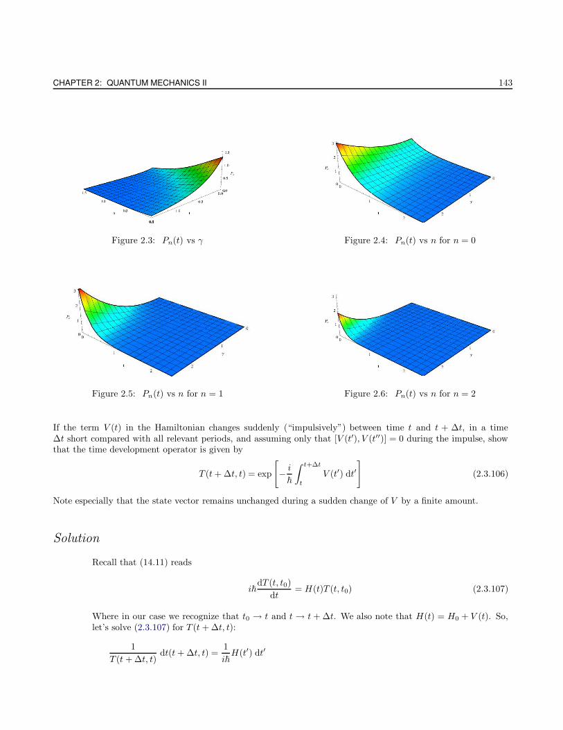
CHAPTER 2: QUANTUM MECHANICS II 143
Figure 2.3: Pn(t) vs γ Figure 2.4: Pn(t) vs n for n = 0
Figure 2.5: Pn(t) vs n for n = 1 Figure 2.6: Pn(t) vs n for n = 2
If the term V (t) in the Hamiltonian changes suddenly (“impulsively”) between time t and t + ∆t, in a time∆t short compared with all relevant periods, and assuming only that [V (t′), V (t′′)] = 0 during the impulse, showthat the time development operator is given by
T (t+ ∆t, t) = exp
[− i
~
∫ t+∆t
t
V (t′) dt′]
(2.3.106)
Note especially that the state vector remains unchanged during a sudden change of V by a finite amount.
Solution
Recall that (14.11) reads
i~dT (t, t0)
dt= H(t)T (t, t0) (2.3.107)
Where in our case we recognize that t0 → t and t → t + ∆t. We also note that H(t) = H0 + V (t). So,let’s solve (2.3.107) for T (t + ∆t, t):
1
T (t + ∆t, t)dt(t+ ∆t, t) =
1
i~H(t′) dt′
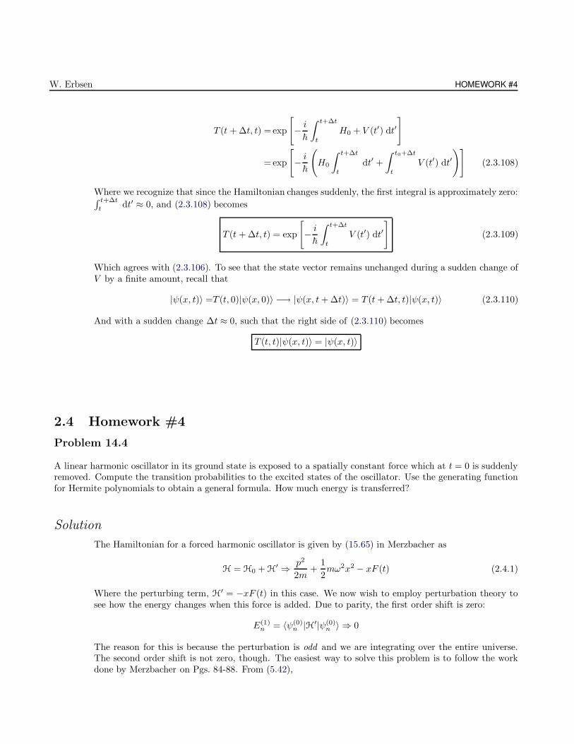
W. Erbsen HOMEWORK #4
T (t + ∆t, t) = exp
[− i
~
∫ t+∆t
t
H0 + V (t′) dt′]
=exp
[− i
~
(H0
∫ t+∆t
t
dt′ +
∫ t0+∆t
t
V (t′) dt′)]
(2.3.108)
Where we recognize that since the Hamiltonian changes suddenly, the first integral is approximately zero:∫ t+∆t
tdt′ ≈ 0, and (2.3.108) becomes
T (t + ∆t, t) = exp
[− i
~
∫ t+∆t
t
V (t′) dt′]
(2.3.109)
Which agrees with (2.3.106). To see that the state vector remains unchanged during a sudden change ofV by a finite amount, recall that
|ψ(x, t)〉 =T (t, 0)|ψ(x, 0)〉 −→ |ψ(x, t+ ∆t)〉 = T (t+ ∆t, t)|ψ(x, t)〉 (2.3.110)
And with a sudden change ∆t ≈ 0, such that the right side of (2.3.110) becomes
T (t, t)|ψ(x, t)〉 = |ψ(x, t)〉
2.4 Homework #4
Problem 14.4
A linear harmonic oscillator in its ground state is exposed to a spatially constant force which at t = 0 is suddenlyremoved. Compute the transition probabilities to the excited states of the oscillator. Use the generating functionfor Hermite polynomials to obtain a general formula. How much energy is transferred?
Solution
The Hamiltonian for a forced harmonic oscillator is given by (15.65) in Merzbacher as
H = H0 + H′ ⇒ p2
2m+
1
2mω2x2 − xF (t) (2.4.1)
Where the perturbing term, H′ = −xF (t) in this case. We now wish to employ perturbation theory tosee how the energy changes when this force is added. Due to parity, the first order shift is zero:
E(1)n = 〈ψ(0)
n |H′|ψ(0)n 〉 ⇒ 0
The reason for this is because the perturbation is odd and we are integrating over the entire universe.The second order shift is not zero, though. The easiest way to solve this problem is to follow the workdone by Merzbacher on Pgs. 84-88. From (5.42),
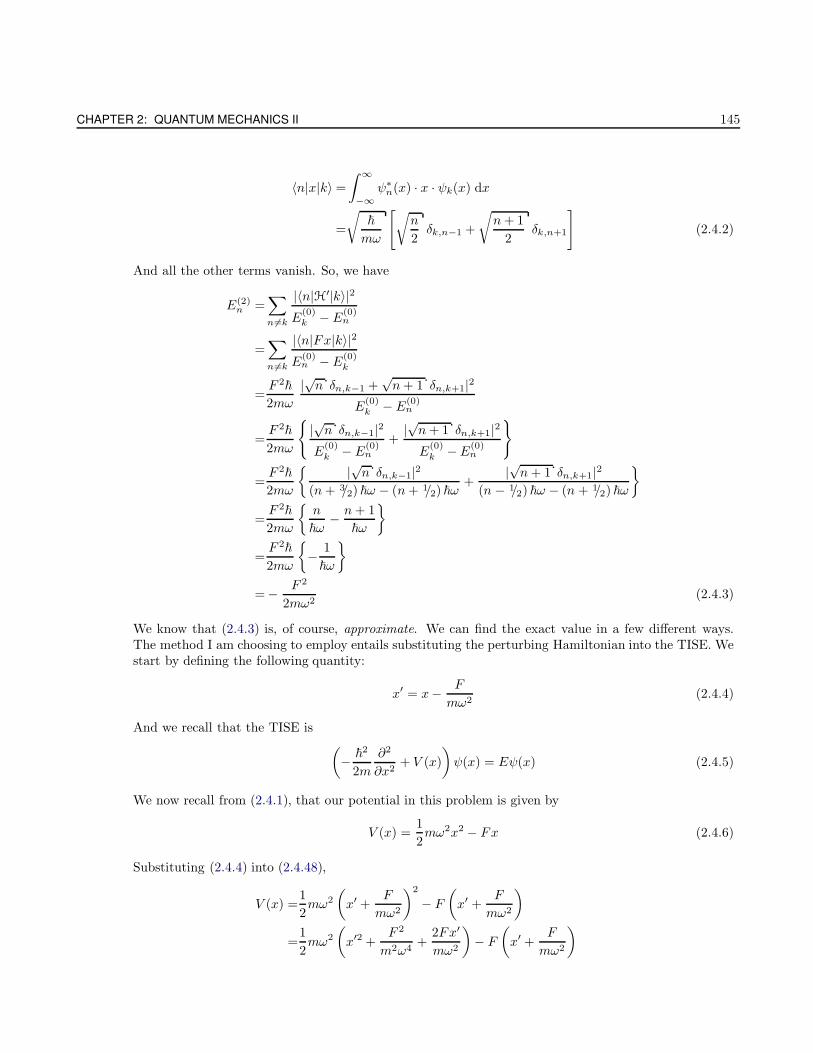
CHAPTER 2: QUANTUM MECHANICS II 145
〈n|x|k〉 =
∫ ∞
−∞ψ∗
n(x) · x · ψk(x) dx
=
√~
mω
[√n
2δk,n−1 +
√n+ 1
2δk,n+1
](2.4.2)
And all the other terms vanish. So, we have
E(2)n =
∑
n 6=k
|〈n|H′|k〉|2
E(0)k − E
(0)n
=∑
n 6=k
|〈n|Fx|k〉|2
E(0)n − E
(0)k
=F 2~
2mω
|√n δn,k−1 +√n+ 1 δn,k+1|2
E(0)k − E
(0)n
=F 2~
2mω
|√n δn,k−1|2
E(0)k − E
(0)n
+|√n+ 1 δn,k+1|2
E(0)k −E
(0)n
=F 2~
2mω
|√n δn,k−1|2(n+ 3/2) ~ω − (n+ 1/2) ~ω
+|√n+ 1 δn,k+1|2
(n − 1/2) ~ω − (n + 1/2) ~ω
=F 2~
2mω
n
~ω− n+ 1
~ω
=F 2~
2mω
− 1
~ω
= − F 2
2mω2(2.4.3)
We know that (2.4.3) is, of course, approximate. We can find the exact value in a few different ways.The method I am choosing to employ entails substituting the perturbing Hamiltonian into the TISE. Westart by defining the following quantity:
x′ = x− F
mω2(2.4.4)
And we recall that the TISE is(− ~2
2m
∂2
∂x2+ V (x)
)ψ(x) = Eψ(x) (2.4.5)
We now recall from (2.4.1), that our potential in this problem is given by
V (x) =1
2mω2x2 − Fx (2.4.6)
Substituting (2.4.4) into (2.4.48),
V (x) =1
2mω2
(x′ +
F
mω2
)2
− F
(x′ +
F
mω2
)
=1
2mω2
(x′2 +
F 2
m2ω4+
2Fx′
mω2
)− F
(x′ +
F
mω2
)
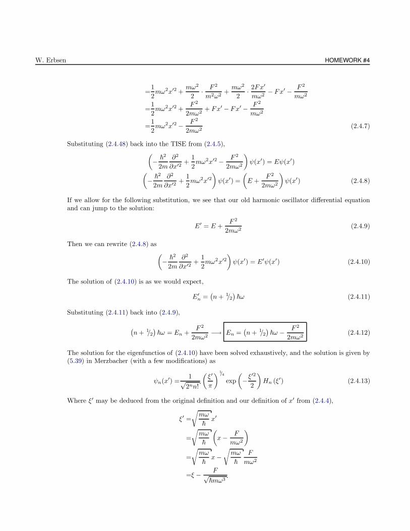
W. Erbsen HOMEWORK #4
=1
2mω2x′2 +
mω2
2· F 2
m2ω2+mω2
2· 2Fx′
mω2− Fx′ − F 2
mω2
=1
2mω2x′2 +
F 2
2mω2+ Fx′ − Fx′ − F 2
mω2
=1
2mω2x′2 − F 2
2mω2(2.4.7)
Substituting (2.4.48) back into the TISE from (2.4.5),
(− ~2
2m
∂2
∂x′2+
1
2mω2x′2 − F 2
2mω2
)ψ(x′) = Eψ(x′)
(− ~2
2m
∂2
∂x′2+
1
2mω2x′2
)ψ(x′) =
(E +
F 2
2mω2
)ψ(x′) (2.4.8)
If we allow for the following substitution, we see that our old harmonic oscillator differential equationand can jump to the solution:
E′ = E +F 2
2mω2(2.4.9)
Then we can rewrite (2.4.8) as
(− ~2
2m
∂2
∂x′2+
1
2mω2x′2
)ψ(x′) = E′ψ(x′) (2.4.10)
The solution of (2.4.10) is as we would expect,
E′n =
(n+ 1/2
)~ω (2.4.11)
Substituting (2.4.11) back into (2.4.9),
(n+ 1/2
)~ω = En +
F 2
2mω2−→ En =
(n+ 1/2
)~ω − F 2
2mω2(2.4.12)
The solution for the eigenfunctios of (2.4.10) have been solved exhaustively, and the solution is given by(5.39) in Merzbacher (with a few modifications) as
ψn(x′) =1√
2nn!
(ξ′
π
) 1/4
exp
(−ξ
′2
2
)Hn (ξ′) (2.4.13)
Where ξ′ may be deduced from the original definition and our definition of x′ from (2.4.4),
ξ′ =
√mω
~x′
=
√mω
~
(x− F
mω2
)
=
√mω
~x−
√mω
~
F
mω2
=ξ − F√~mω3
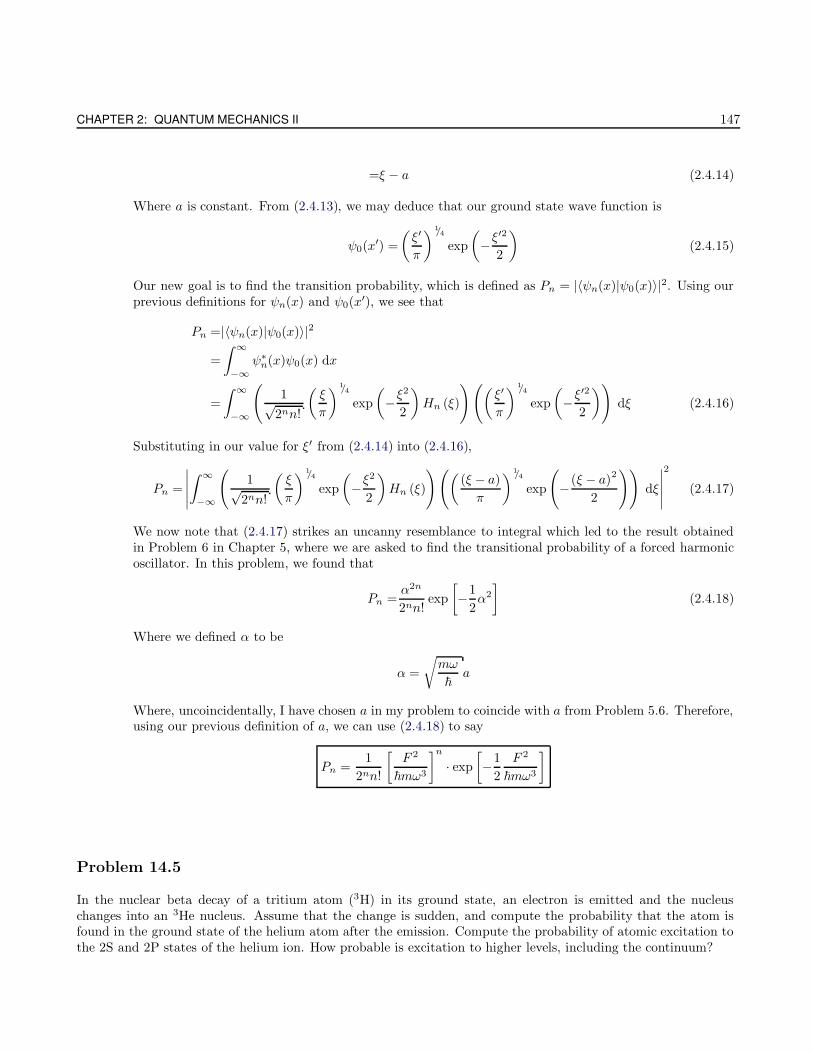
CHAPTER 2: QUANTUM MECHANICS II 147
=ξ − a (2.4.14)
Where a is constant. From (2.4.13), we may deduce that our ground state wave function is
ψ0(x′) =
(ξ′
π
) 1/4
exp
(−ξ
′2
2
)(2.4.15)
Our new goal is to find the transition probability, which is defined as Pn = |〈ψn(x)|ψ0(x)〉|2. Using ourprevious definitions for ψn(x) and ψ0(x
′), we see that
Pn =|〈ψn(x)|ψ0(x)〉|2
=
∫ ∞
−∞ψ∗
n(x)ψ0(x) dx
=
∫ ∞
−∞
(1√
2nn!
(ξ
π
) 1/4
exp
(−ξ
2
2
)Hn (ξ)
)((ξ′
π
) 1/4
exp
(−ξ
′2
2
))dξ (2.4.16)
Substituting in our value for ξ′ from (2.4.14) into (2.4.16),
Pn =
∣∣∣∣∣
∫ ∞
−∞
(1√
2nn!
(ξ
π
) 1/4
exp
(−ξ
2
2
)Hn (ξ)
)(((ξ − a)
π
)1/4
exp
(−(ξ − a)2
2
))dξ
∣∣∣∣∣
2
(2.4.17)
We now note that (2.4.17) strikes an uncanny resemblance to integral which led to the result obtainedin Problem 6 in Chapter 5, where we are asked to find the transitional probability of a forced harmonicoscillator. In this problem, we found that
Pn =α2n
2nn!exp
[−1
2α2
](2.4.18)
Where we defined α to be
α =
√mω
~a
Where, uncoincidentally, I have chosen a in my problem to coincide with a from Problem 5.6. Therefore,using our previous definition of a, we can use (2.4.18) to say
Pn =1
2nn!
[F 2
~mω3
]n
· exp
[−1
2
F 2
~mω3
]
Problem 14.5
In the nuclear beta decay of a tritium atom (3H) in its ground state, an electron is emitted and the nucleuschanges into an 3He nucleus. Assume that the change is sudden, and compute the probability that the atom isfound in the ground state of the helium atom after the emission. Compute the probability of atomic excitation tothe 2S and 2P states of the helium ion. How probable is excitation to higher levels, including the continuum?
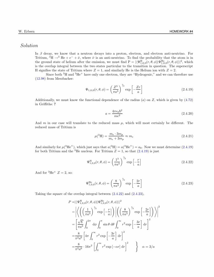
W. Erbsen HOMEWORK #4
Solution
In β decay, we know that a neutron decays into a proton, electron, and electron anti-neutrino. ForTritium, 3H →3 He + e− + ν, where ν is an anti-neutrino. To find the probability that the atom is inthe ground state of helium after the emission, we must find P = |〈ΨH
1,0,0(r, θ, φ)|ΨHe1,0,0(r, θ, φ)〉|2, which
is the overlap integral between the two states particular to the transition in question. The superscriptH signifies the state of Tritium where Z = 1, and similarly He is the Helium ion with Z = 2.
Since both 3H and 3He+ have only one electron, they are “Hydrogenic,” and we can therefore use(12.98) from Merzbacher:
Ψ1,0,0(r, θ, φ) =
(Z3
πa3
) 1/2
exp
[−Zra
](2.4.19)
Additionally, we must know the functional dependence of the radius (a) on Z, which is given by (4.72)in Griffiths: ?
a =4πε0~
2
me2(2.4.20)
And m in our case will translate to the reduced mass µ, which will most certainly be different. Thereduced mass of Tritium is
µ(3H) =me · 3mp
me + 3mp≈ me (2.4.21)
And similarly for µ(3He+), which just says that a(3H) = a(3He+) = a0. Now we must determine (2.4.19)for both Tritium and the 3He nucleus. For Tritium Z = 1, so that (2.4.19) is just
ΨH1,0,0(r, θ, φ) =
(13
πa3
) 1/2
exp[− ra
](2.4.22)
And for 3He+ Z = 2, so:
ΨHe1,0,0(r, θ, φ) =
(8
πa3
)1/2
exp
[−2r
a
](2.4.23)
Taking the square of the overlap integral between (2.4.22) and (2.4.23),
P =|〈ΨH1,0,0(r, θ, φ)|ΨHe
1,0,0(r, θ, φ)〉|2
=
∣∣∣∣∣
⟨((1
πa3
) 1/2
exp[− ra
]) ∣∣∣∣∣
((8
πa3
) 1/2
exp
[−2r
a
])⟩∣∣∣∣∣
2
=
[√8
πa3
∫ 2π
0
dφ
∫ π
0
sin θ dθ
∫ ∞
0
r2 exp
[−3r
a
]dr
]2
=8
π2a6
[4π
∫ ∞
0
r2 exp
[−3r
a
]dr
]2
=8
π2a6· 16π2
[∫ ∞
0
r2 exp [−αr] dr
]2 α = 3/a
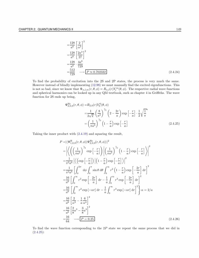
CHAPTER 2: QUANTUM MECHANICS II 149
=128
a6
[2
α3
]2
=128
a6
[2a3
27
]2
=128
a6· 4a6
729
=512
729−→ P ≈ 0.702332 (2.4.24)
To find the probability of excitation into the 2S and 2P states, the process is very much the same.However instead of blindly implementing (12.98) we must manually find the excited eigenfunctions. Thisis not so bad, since we know that Ψn,l,m(r, θ, φ) = Rn,l(r)Y
ml (θ, φ). The respective radial wave functions
and spherical harmonics can be looked up in any QM textbook, such as chapter 4 in Griffiths. The wavefunction for 2S ends up being,
ΨHe2,0,0(r, θ, φ) =R2,0(r)Y
00 (θ, φ)
=1
2√
2
(8
a3
)1/2 (2 − 2r
a
)exp
[− ra
]· 1
2
√1
π
=
(1
πa3
) 1/2 (1 − r
a
)exp
[− ra
](2.4.25)
Taking the inner product with (2.4.19) and squaring the result,
P =|〈ΨH1,0,0(r, θ, φ)|ΨHe
2,0,0(r, θ, φ)〉|2
=
∣∣∣∣∣
⟨((1
πa3
)1/2
exp[− ra
]) ∣∣∣∣∣
(1
πa3
)1/2 (1 − r
a
)exp
[− ra
]⟩∣∣∣∣∣
2
=1
π2a6
∣∣∣⟨(
exp[− ra
]) ∣∣∣(1 − r
a
)exp
[− ra
]⟩∣∣∣2
=1
π2a6
[∫ 2π
0
dφ
∫ π
0
sin θ dθ
∫ ∞
0
r2(1 − r
a
)exp
[−2r
a
]dr
]2
=16
a6
[∫ ∞
0
r2 exp
[−2r
a
]dr − 1
a
∫ ∞
0
r3 exp
[−2r
a
]dr
]2
=16
a6
[∫ ∞
0
r2 exp [−αr] dr − 1
a
∫ ∞
0
r3 exp [−αr] dr
]2α = 2/a
=16
a6
[2
α3− 1
a
6
α4
]2
=16
a6
[2
8a3 − 3
8a3
]2
=16
64−→ P = 0.25 (2.4.26)
To find the wave function corresponding to the 2P state we repeat the same process that we did in(2.4.25):
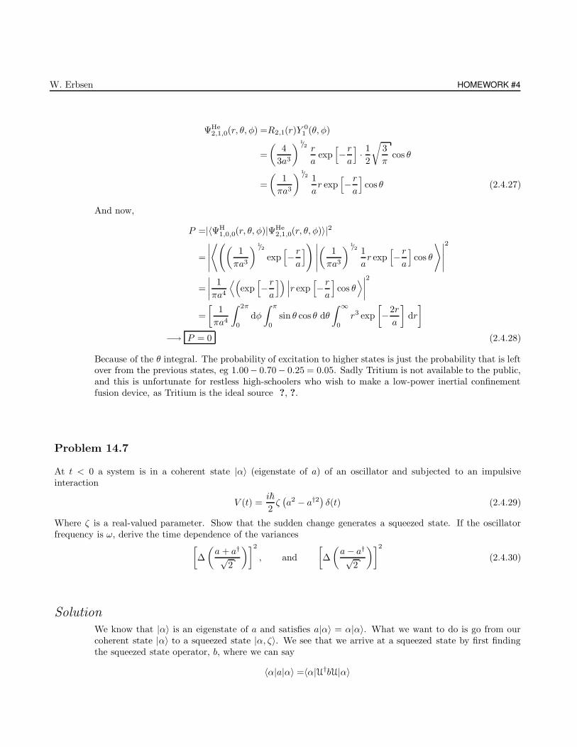
W. Erbsen HOMEWORK #4
ΨHe2,1,0(r, θ, φ) =R2,1(r)Y
01 (θ, φ)
=
(4
3a3
) 1/2 r
aexp
[− ra
]· 1
2
√3
πcos θ
=
(1
πa3
)1/2 1
ar exp
[− ra
]cos θ (2.4.27)
And now,
P =|〈ΨH1,0,0(r, θ, φ)|ΨHe
2,1,0(r, θ, φ)〉|2
=
∣∣∣∣∣
⟨((1
πa3
) 1/2
exp[− ra
]) ∣∣∣∣∣
(1
πa3
) 1/2 1
ar exp
[− ra
]cos θ
⟩∣∣∣∣∣
2
=
∣∣∣∣1
πa4
⟨(exp
[− ra
]) ∣∣∣r exp[− ra
]cos θ
⟩∣∣∣∣2
=
[1
πa4
∫ 2π
0
dφ
∫ π
0
sin θ cos θ dθ
∫ ∞
0
r3 exp
[−2r
a
]dr
]
−→ P = 0 (2.4.28)
Because of the θ integral. The probability of excitation to higher states is just the probability that is leftover from the previous states, eg 1.00− 0.70− 0.25 = 0.05. Sadly Tritium is not available to the public,and this is unfortunate for restless high-schoolers who wish to make a low-power inertial confinementfusion device, as Tritium is the ideal source ?, ?.
Problem 14.7
At t < 0 a system is in a coherent state |α〉 (eigenstate of a) of an oscillator and subjected to an impulsiveinteraction
V (t) =i~
2ζ(a2 − a†2
)δ(t) (2.4.29)
Where ζ is a real-valued parameter. Show that the sudden change generates a squeezed state. If the oscillatorfrequency is ω, derive the time dependence of the variances
[∆
(a + a†√
2
)]2, and
[∆
(a− a†√
2
)]2(2.4.30)
Solution
We know that |α〉 is an eigenstate of a and satisfies a|α〉 = α|α〉. What we want to do is go from ourcoherent state |α〉 to a squeezed state |α, ζ〉. We see that we arrive at a squeezed state by first findingthe squeezed state operator, b, where we can say
〈α|a|α〉 =〈α|U†bU|α〉
CHAPTER 2: QUANTUM MECHANICS II 151
=〈α, ζ|b|α, ζ〉 (2.4.31)
The easiest way to find b would be to utilize some identities made available by Merzbacher on pgs. 39-40.He says that if
f(λ) = eλABe−λA
Then we can write
f(λ) = B cosh λ√β +
[A,B]√β
sinhλ√β (2.4.32)
Which we can use only if β is constant, and the operators A and B satisfy [A, [A,B]] = βB. In our case,f(λ) → b(ζ), and A = (a2 − a†2) and B = a. To find out if we can use (2.4.32):
[A,B] =[(a2 − a†2), a]
=[a2, a]− [a†2, a]
= − [a†2, a]
= − a†[a†, a]− [a†, a]a†
= − a†(−1) − (−1)a†
=2a† (2.4.33)
[A, [A,B]] =[(a2 − a†2), 2a†]
=2([a2, a†]− [a†2a†]
)
=2(a[a, a†] + [a, a†]a
)
=4a (2.4.34)
It seems that we can in fact use (2.4.32), since both of our conditions are satisfied with λ = −ζ/2 andβ = 4. We now have,
b(ζ) =a coshλ√β +
[A,B]√β
sinhλ√β
=a cosh−ζ/2√
4 +2a†√
4sinh−ζ/2
√4
=a cosh ζ + a† sinh ζ
=a cosh ζ − a† sinh ζ (2.4.35)
Following Merzbacher’s lead on pgs. 230-231, we define λ = cosh ζ and ν = sinh ζ, where λ here isdifferent than the one used before. We can now rewrite (2.4.35):
b = λa+ νa† (2.4.36)
And taking the Hermitian conjugate,
b† = λa† + νa (2.4.37)
W. Erbsen HOMEWORK #4
Since both λ and ν are real. Inverting these two equations
a = λb− νb† (2.4.38)
a† = λb† − νb (2.4.39)
And we can now write
1√2〈α|a|α〉 =
1√2〈α, ζ|b|α, ζ〉
=1√2〈α, ζ|λa+ νa†|α, ζ〉 (2.4.40)
1√2〈α|a†|α〉 =
1√2〈α, ζ|b†|α, ζ〉
=1√2〈α, ζ|λa† + νa|α, ζ〉 (2.4.41)
So, we can say that the impulsive action of (2.4.29) generates a squeezed state . We can find the vari-
ances from (2.4.30) by recalling that we can write
[∆
(a+ a†√
2
)]2=
1
2
[〈α, ζ|
(a+ a†
)2|α, ζ〉 − 〈α, ζ|(a+ a†
)|α, ζ〉2
](2.4.42a)
[∆
(a− a†√
2
)]2=
1
2
[〈α, ζ|
(a− a†
)2|α, ζ〉 − 〈α, ζ|(a− a†
)|α, ζ〉2
](2.4.42b)
We can evaluate (2.4.42a) and (2.4.42b) according to the previous formulas laid out in this problem.Unfortunately, I did not have time as I have been preparing a presentation for WildCorn. The frameworkhas been laid out, the rest of this problem is very straightforward.
Exercise 15.5
From the definition (15.31) of the propagator and the Hermitian character of the Hamiltonian, show that
K(r′, r; t′, t) = K∗(r, r′; t, t′) (2.4.43)
linking the transition amplitude that reverses the dynamical development between spacetime points (r, t) and(r′, t′) to the original propagator.
Solution
We first recall (15.31), which states
K(r, r′; t, t′) = 〈r|T (t, t′)|r′〉 (2.4.44)
CHAPTER 2: QUANTUM MECHANICS II 153
Where the time evolution operator is given by (14.41) as
T (t, t′) = exp
[− i
~H(t− t′)
](2.4.45)
Substituting (2.4.45) into (2.4.44) (letting ~ → 1 for convenience),
K(r, r′; t, t′) =〈r|e−iH(t−t′)|r′〉 ⇒(〈r|e−iHt
)(eiHt′ |r′〉
)(2.4.46)
We now take the complex conjugate of both sides of (2.4.46),
K∗(r, r′; t, t′) =[(
〈r|e−iHt)(
eiHt′ |r′〉)]∗
⇒(eiHt′ |r′〉
)∗ (〈r|e−iHt
)∗(2.4.47)
Recalling the Hermitian property of the Hamiltonian H∗ = H†, we can rewrite (2.4.47) as
K∗(r, r′; t, t′) =(〈r′|e−iHt′
)(eiHt|r〉
)⇒ 〈r′|e−iH(t′−t)|r〉 (2.4.48)
Going back to (2.4.46), if we interchange r and r′ and also t and t′, then (2.4.46) becomes
K(r′, r; t′, t) =(〈r′|e−iHt′
)(eiHt|r〉
)⇒ 〈r′|e−iH(t′−t)|r〉 (2.4.49)
We now see that (2.4.49) is equal to (2.4.48), and we can now say
K(r′, r; t′, t) = K∗(r, r′; t, t′)
Exercise 15.8
Verify that (15.48) solves the time-dependent Schrodinger equation and agrees with the initial contition (15.32). Ifthe initial (t′ = 0) state of a free particle is represented by ψ(x, 0) = eik0x, verify that (15.35) produces the usualplane wave.
Solution
Equation (15.48) reads
K(x; x′; t− t′) =
√m
2πi~(t − t′)exp
m(x − x′)2
2i~(t − t′)
(2.4.50)
We want to use this in the time-dependent Schrodinger equation (15.33):
i~∂
∂tK(r, r′; t, t′) =
[− ~2
2m
(∇− iq
~cA
)2
+ V
]K(r, r′; t, t′) (2.4.51)
The LHS of (2.4.51) is
W. Erbsen HOMEWORK #4
i~∂
∂tK(r, r′; t, t′) =i~
∂
∂t
[√m
2πi~(t − t′)exp
m(x− x′)2
2i~(t − t′)
]
=−m(x − x′)2 + i(t − t′)~
2(t− t′)2·(− im
2π~t − 2πt′~
)1/2
· exp
[− im(x − x′)2
2(t − t′)~
](2.4.52)
While the RHS of (2.4.51) is
[− ~2
2m
(∇− iq
~cA
)2
+ V
]K(r, r′; t, t′) =
[− ~2
2m
(∇− iq
~cA
)2
+ V
]√m
2πi~(t − t′)exp
m(x − x′)2
2i~(t− t′)
= − ~2
2m∇2
√m
2πi~(t − t′)exp
m(x− x′)2
2i~(t − t′)
=−m(x − x′)2 + i(t − t′)~
2(t− t′)2·(− im
2π~t − 2πt′~
) 1/2
· exp
[− im(x − x′)2
2(t− t′)~
](2.4.53)
Since we have a free particle and A = 0 and V = 0. All derivatives were computed with Mathematica.We do notice, however that the left side of (2.4.51), (2.4.52) is equal to the right side, (2.4.53), therefore(2.4.50) solves the time-dependent Schrodinger equation.
We are now asked to verify that this agrees with the initial condition given by (15.32), which says:
K(r, r′; t, t) = δ(r − r′) (2.4.54)
Which clearly satisfies the TDSE for t−t′ −→ t−t = 0 because of the completeness of the eigenfunctions:
K(r, r′; t, t′) =
∞∑
n=0
ψ∗n(r′)ψn(r)e−iEnt/~ (2.4.55)
And in our case,
K(r, r′; t, t) =
∞∑
n=0
ψ∗n(r′)ψn(r) = δ(r − r′) (2.4.56)
For the last part of the question, (15.35) reads
ψ(r, t) =
∫K(r, r′; t, t′)ψ(r′, t′)d3r′ (2.4.57)
Where in our case t′ = 0, ψ(x, 0) = eik0x and K(r, r′; t, t′) is given by (2.4.50). So, (2.4.57) becomes:
ψ(r, t) =
∫ ∞
−∞K(r, r′; t, 0)ψ(r′, 0)d3r′
=
∫ ∞
−∞
√m
2πi~texp
m(x− x′)2
2i~t
· eik0x′
dx′
=
∫ ∞
−∞
√m
2πi~texp
m(x− x′)2
2i~t+ ik0x
′
dx′
CHAPTER 2: QUANTUM MECHANICS II 155
=
√m
2πi~t
∫ ∞
−∞exp
m(x2 − 2xx′ − x′2)
2i~t+ ik0x
′
dx′
=
√m
2πi~t
∫ ∞
−∞exp
mx2
2i~t− mxx′
i~t− mx′2
2i~t+ ik0x
′
dx′
=
√m
2πi~t
∫ ∞
−∞exp
−mx
′2
2i~t− mxx′
i~t+mx2
2i~t+ ik0x
′
dx′
=
√m
2πi~t
∫ ∞
−∞exp
(− m
2i~t
)x′2 +
(ik0 −
mx
i~t
)x′ +
(mx2
2i~t
)dx′
=
√m
2πi~t
∫ ∞
−∞exp
ax′2 + bx′ + c
dx′
=
√m
2πi~t
√π
−a exp
[−b24a
+ c
](2.4.58)
Where I have set
a = − m
2i~t(2.4.59a)
b =ik0 −mx
i~t(2.4.59b)
c =mx2
2i~t(2.4.59c)
We now wish to evaluate (2.4.58) one bit at a time. The first factor is
√π
−a =
√π · 2i~t
m⇒√
2πi~t
m(2.4.60)
The exponential term becomes
exp
[−b24a
+ c
]=exp
[−(ik0 − mx
i~t
)2
4(− m
2i~t
) +mx2
2i~t
]
=exp
[1
4· 2i~t
m
(−k2
0 − 2mxk0
~t+m2x2
~2t2
)+mx2
2i~t
]
=exp
[− ik
20~t
2m− ixk0 +
imx2
2~t− imx2
2~t
]
=exp
[− ik0
2m(k0~t + 2mx)
](2.4.61)
Substituting (2.4.60) and (2.4.61) back into (2.4.58),
ψ(r, t) =
√m
2πi~t·√
2πi~t
mexp
[− ik0
2m(k0~t+ 2mx)
]−→ ψ(r, t) = exp
[− ik0
2m(k0~t + 2mx)
]
(2.4.62)
Which is indeed a plane wave.
W. Erbsen HOMEWORK #4
Exercise 15.9
Calculate |ψ(x, t)|2 from (15.50) and show that the wave packet moves uniformly and at the same time spreads sothat
(∆x)2t = (∆x)
20
[1 +
~2t2
4m2 (∆x)40
](2.4.63)
Solution
Equation (15.50) reads:
ψ(x, t) = [2π(∆x)20]−1/4 ·
[1 +
i~t
2m(∆x)20
]−1/2
· exp
− x2
4(∆x)20+ ik0x− ik2
0~t2m
1 + i~t2m(∆x)20
(2.4.64)
To make calculating |ψ(x, t)|2 from (2.4.64) easier recall that if we have (a+ ib)/(c + id), then
a+ ib
c+ id· c − id
c − id⇒ (a+ ib)(c − id)
c2 + d2(2.4.65)
Furthermore we remember that if f(x) = exp (e+ if) then |f(x)| = exp (e− if) ·exp (e+ if) = exp (2e),so in further calculations I will recognize that the imaginary phase cancels out ahead of time to simplifythe calculations. So, we have:
|ψ(x, t)|2 =
∣∣∣∣∣∣[2π(∆x)20]
−1/4 ·[1 +
i~t
2m(∆x)20
]−1/2
· exp
− x2
4(∆x)20+ ik0x− ik2
0~t2m
1 + i~t2m(∆x)20
∣∣∣∣∣∣
2
=
∣∣∣∣∣[2π(∆x)20]−1/4 ·
[1 +
i~t
2m(∆x)20
]−1/2∣∣∣∣∣
2
︸ ︷︷ ︸|ψI|2
·
∣∣∣∣∣∣exp
− x2
4(∆x)20+ ik0x− ik2
0~t2m
1 + i~t2m(∆x)20
∣∣∣∣∣∣
2
︸ ︷︷ ︸|ψII |2
(2.4.66)
Such that
|ψI|2 =
∣∣∣∣∣[2π(∆x)20]−1/4 ·
[1 +
i~t
2m(∆x)20
]−1/2∣∣∣∣∣
2
⇒ [2π(∆x)20]−1/2 ·
[1 +
~2t2
4m2(∆x)40
]−1/2
(2.4.67)
And also
|ψII |2 =
∣∣∣∣∣∣exp
− x2
4(∆x)20+ ik0x− ik2
0~t2m
1 + i~t2m(∆x)20
∣∣∣∣∣∣
2
=exp
− x2
4(∆x)20− ik0x+ ik2
0~t2m
1 − i~t2m(∆x)20
+− x2
4(∆x)20+ ik0x− ik2
0~t2m
1 + i~t2m(∆x)20
CHAPTER 2: QUANTUM MECHANICS II 157
=exp
− x2
4(∆x)20− ik0x+ ik2
0~t2m
1 − i~t2m(∆x)20
·1 + i~t
2m(∆x)20
1 + i~t2m(∆x)20
+− x2
4(∆x)20+ ik0x− ik2
0~t2m
1 + i~t2m(∆x)20
·1 − i~t
2m(∆x)20
1 − i~t2m(∆x)20
=exp
− x2
4(∆x)20+ k0~xt
2m(∆x)20− k2
0~2t2
4m2(∆x)20− x2
4(∆x)20+ k0~xt
2m(∆x)20− k2
0~2t2
4m2(∆x)20
1 + ~2t2
4m(∆x)40
=exp
− x2
2(∆x)20+ k0~xt
m(∆x)20− k2
0~2t2
2m2(∆x)20
1 + ~2t2
4m(∆x)40
=exp
−
x2
2 + k0~xtm − k2
0~2t2
2m2
(∆x)20
(1 + ~2t2
4m(∆x)40
)
(2.4.68)
Combining (2.4.67) and (2.4.68),
|ψ(x, t)|2 =|ψI|2|ψII |2
=[2π(∆x)20]−1/2 ·
[1 +
~2t2
4m2(∆x)40
]−1/2
· exp
(
k0~tm − x
) (−k0~t
2m + x2
)
(∆x)20
(1 + ~2t2
4m(∆x)40
)
(2.4.69)
Which is the answer. By graphing this we can see that this does indeed move uniformly and spreads intime. If we substitute (2.4.63) into (2.4.69),
|ψ(x, t)|2 = [2π(∆x)2t ]−1/2 · exp
[(k0~t/m− x) (−k0~t/(2m) + x/2)
(∆x)2t
](2.4.70)
With the definition of (∆x)t provided by (2.4.63), (2.4.70) is very clearly Gaussian (not that it didn’tlook that way before). Please see attached Mathematica printout for plots.
Exercise 15.13
For the harmonic oscillator, derive ψ(x, t) directly from ψ(x, 0) by expanding the initial wave function, whichrepresents a displaced ground state as in (15.60), in terms of stationary states. Use the generating function (5.33)to obtain the expansion coefficients and again to sum the expansion. Rederive (15.61).
Solution
Using the definition of the propagator from (15.59),
K(x, x′; t) =
α︷ ︸︸ ︷(mω
2πi~ sin(ωt)
) 1/2
exp
− mω
2i~ sin(ωt)(x2 cos(ωt) − 2xx′ + x′2 cos(ωt))
W. Erbsen HOMEWORK #4
=α exp
− mω
2i~ sin(ωt)(x2 cos(ωt) − 2xx′ + x′2 cos(ωt))
(2.4.71)
We can find ψ(x, t) using
ψ(x, t) =
∫ ∞
−∞K(x, x′; t)ψ(x′, 0) dx′
=αN
∫ ∞
−∞exp
− mω
2i~ sin(ωt)(x2 cos(ωt) − 2xx′ + x′2 cos(ωt))
· exp
−mω
2~(x′ − x0)
2
dx′
=αN
∫ ∞
−∞exp
− mω
2i~ sin(ωt)(x2 cos(ωt) − 2xx′ + x′2 cos(ωt)) − mω
2~(x′ − x0)
2
dx′
=αN
∫ ∞
−∞exp
mω
2~
[−x
2 cos(ωt)
i sin(ωt)+
2xx′
i sin(ωt)− x′2 cos(ωt)
i sin(ωt)− (x′ − x0)
2
]dx′
=αN
∫ ∞
−∞exp
mω
2~
[−x
2 cos(ωt)
i sin(ωt)+
2xx′
i sin(ωt)− x′2 cos(ωt)
i sin(ωt)− x′2 + 2x′x0 − x2
0
]dx′
=αN
∫ ∞
−∞exp
−mωx
2 cos(ωt)
2i~ sin(ωt)+
2mωxx′
2i~ sin(ωt)− mωx′2 cos(ωt)
2i~ sin(ωt)
−mωx′2
2~+
2mωx′x0
2~− mωx2
0
2~
dx′
=αN
∫ ∞
−∞exp
−mωx
′2
2~− mωx′2 cos(ωt)
2i~ sin(ωt)+
mωxx′
i~ sin(ωt)+mωx′x0
~
−mωx2 cos(ωt)
2i~ sin(ωt)− mωx2
0
2~
dx′
=αN
∫ ∞
−∞exp
(−mω
2~− mω cos(ωt)
2i~ sin(ωt)
)x′2 +
(mωx
i~ sin(ωt)+mωx0
~
)x′
+
(−mωx
2 cos(ωt)
2i~ sin(ωt)− mωx2
0
2~
)dx′ (2.4.72)
Where we set
a = − mω
2~− mω cos(ωt)
2i~ sin(ωt)= −mω
2~
(1 +
cos(ωt)
i sin(ωt)
)(2.4.73)
b =mωx
i~ sin(ωt)+mωx0
~=mω
~
(x
i sin(ωt)+ x0
)(2.4.74)
c = − mωx2 cos(ωt)
2i~ sin(ωt)− mωx2
0
2~= −mω
2~
(x2 cos(ωt)
i sin(ωt)+ x2
0
)(2.4.75)
Such that (2.4.72) becomes
ψ(x, t) =αN
∫ ∞
−∞exp
ax′2 + bx′ + c
dx′
=αN
[√π
−a exp
[− b2
4a+ c
]](2.4.76)
Where we have
CHAPTER 2: QUANTUM MECHANICS II 159
√π
−a =
[π
(mω
2~
(1 +
cos(ωt)
i sin(ωt)
))−1]1/2
=
[π
(mω
2~
(i sin(ωt) + cos(ωt)
i sin(ωt)
))−1] 1/2
=
[2π~
mω
(i sin(ωt)
i sin(ωt) + cos(ωt)
)]1/2
(2.4.77)
And also, we can say that
exp
[− b2
4a+ c
]= exp
[mω
~
(x
i sin(ωt)+ x0
)]2· 1
4
[mω
2~
(1 +
cos(ωt)
i sin(ωt)
)]−1
− mω
2~
(x2 cos(ωt)
i sin(ωt)+ x2
0
)
We can simplify this further,
exp % =exp
m2ω2
~2
(x
i sin(ωt)+ x0
)2
· 1
4
[mω
2~
(i sin(ωt) + cos(ωt)
i sin(ωt)
)]−1
− mω
2~
(x2 cos(ωt)
i sin(ωt)+ x2
0
)
=exp
mω
2~
(− x2
sin(2ωt)+
2xx0
i sin(ωt)+ x2
0
)(i sin(ωt)
i sin(ωt) + cos(ωt)
)− mω
2~
(x2 cos(ωt)
i sin(ωt)+ x2
0
)
=exp
mω
2~
[(− x2
sin(2ωt)+
2xx0
i sin(ωt)+ x2
0
)(i sin(ωt)
i sin(ωt) + cos(ωt)
)−(x2 cos(ωt)
i sin(ωt)+ x2
0
)]
=exp
mω
2~
[(− ix2
sin(ωt)+ 2xx0 + ix2
0 sin(ωt)
)(1
i sin(ωt) + cos(ωt)
)−(x2 cos(ωt)
i sin(ωt)+ x2
0
)]
=exp
mω
2~
−
ix2
sin(ωt)+ 2xx0 + ix2
0 sin(ωt)
cos(ωt) + i sin(ωt)· (cos(ωt) − i sin(ωt))
(cos(ωt) − i sin(ωt))−(x2 cos(ωt)
i sin(ωt)+ x2
0
)
=exp
mω
2~
−
ix2 cos(ωt)sin(ωt)
+ 2xx0 cos(ωt) + ix20 sin(ωt) cos(ωt) − x2 − 2ixx0 sin(ωt) + x2
0 sin(2ωt)
cos(2ωt) + sin(2ωt)−
−x2 cos(ωt)
i sin(ωt)− x2
0
]
=exp
mω
2~
[− ix
2 cos(ωt)
sin(ωt)+ 2xx0 cos(ωt) + ix2
0 sin(ωt) cos(ωt) − x2 − 2ixx0 sin(ωt) + x20 sin(2ωt)−
−x2 cos(ωt)
i sin(ωt)− x2
0
]
=expmω
2~
[2xx0 cos(ωt) + ix2
0 sin(ωt) cos(ωt) − x2 − 2ixx0 sin(ωt) + x20 sin(2ωt) − x2
0
]
=exp
mω
2~
[2xx0 cos(ωt) +
ix20 sin(2ωt)
2− x2 − 2ixx0 sin(ωt) + x2
0
(1 − cos(2ωt)
)− x2
0
]
=exp
mω
2~
[2xx0 cos(ωt) +
ix20 sin(2ωt)
2− x2 − 2ixx0 sin(ωt) − x2
0 cos(2ωt)
]
W. Erbsen HOMEWORK #4
=exp
mω
2~
[−x2 + 2xx0 cos(ωt) − x2
0 cos(2ωt) − 2ixx0 sin(ωt) +ix2
0 sin(2ωt)
2
]
=exp
−mω
2~
[x2 − 2xx0 cos(ωt) + x2
0 cos(2ωt)]− mωixx0 sin(ωt)
~+imωx2
0 sin(2ωt)
4~
=exp
−mω
2~(x− x0 cos(ωt))
2 − mωixx0 sin(ωt)
~+imωx2
0 sin(2ωt)
4~
=exp
−mω
2~(x− x0 cos(ωt))2 − i
(mωxx0 sin(ωt)
~− mωx2
0 sin(2ωt)
4~
)(2.4.78)
Going back to (2.4.76), implementing (2.4.77) (keeping (2.4.78) arbitrary for the time being), and sub-stituting back in our value for α,
ψ(x, t) =N
(mω
2πi~ sin(ωt)
) 1/2 √ π
−a exp
[− b2
4a+ c
]
=N
(mω
2πi~ sin(ωt)
) 1/2
·[2π~
mω
(i sin(ωt)
cos(ωt) + i sin(ωt)
)]1/2
exp
[− b2
4a+ c
]
=N
[mω
2πi~ sin(ωt)· 2π~
mω
(i sin(ωt)
cos(ωt) + i sin(ωt)
)] 1/2
exp
[− b2
4a+ c
]
=N
[1
i sin(ωt)
(i sin(ωt)
cos(ωt) + i sin(ωt)
)]1/2
exp
[− b2
4a+ c
]
=N
(1
cos(ωt) + i sin(ωt)
)1/2
exp
[− b2
4a+ c
]
=N
(1
(eiωt) + eiωt))/2
)+ i(eiωt) − eiωt))/(2i)
)1/2exp
[− b2
4a+ c
]
=N
(1
eiωt)/2 + e−iωt)/2 + eiωt)/2 − e−iωt)/2
)1/2
exp
[− b2
4a+ c
]
=N
(1
eiωt)
)1/2
exp
[− b2
4a+ c
]
=Ne−iωt)/2 exp
[− b2
4a+ c
](2.4.79)
Now substituting (2.4.78) into (2.4.79),
ψ(x, t) =Ne−iωt)2 exp
−mω
2~(x− x0 cos(ωt))
2 − i(mω
~xx0 sin(ωt) − mω
4~x2
0 sin(2ωt))
=N exp
−mω
2~(x− x0 cos(ωt))2 − i
(mω~xx0 sin(ωt) − mω
4~x2
0 sin(2ωt))− iω
2t
=N exp−mω
2~(x− x0 cos(ωt))
2 − i(ω
2t +
mω
~xx0 sin(ωt) − mω
4~x2
0 sin(2ωt))
(2.4.80)
Such that we finally arrive at
ψ(x, t) = N exp−mω
2~(x− x0 cos(ωt))
2 − i(ω
2t+
mω
~xx0 sin(ωt) − mω
4~x2
0 sin(2ωt))
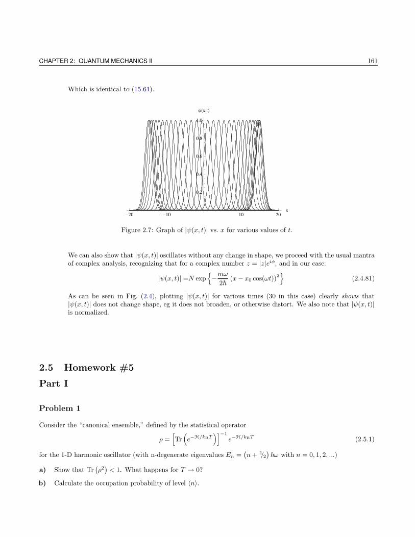
CHAPTER 2: QUANTUM MECHANICS II 161
Which is identical to (15.61).
-20 -10 10 20x
0.2
0.4
0.6
0.8
1.0
ΨHx,tL
Figure 2.7: Graph of |ψ(x, t)| vs. x for various values of t.
We can also show that |ψ(x, t)| oscillates without any change in shape, we proceed with the usual mantraof complex analysis, recognizing that for a complex number z = |z|eiφ, and in our case:
|ψ(x, t)| =N exp−mω
2~(x− x0 cos(ωt))
2
(2.4.81)
As can be seen in Fig. (2.4), plotting |ψ(x, t)| for various times (30 in this case) clearly shows that|ψ(x, t)| does not change shape, eg it does not broaden, or otherwise distort. We also note that |ψ(x, t)|is normalized.
2.5 Homework #5
Part I
Problem 1
Consider the “canonical ensemble,” defined by the statistical operator
ρ =[Tr(e−H/kBT
)]−1
e−H/kBT (2.5.1)
for the 1-D harmonic oscillator (with n-degenerate eigenvalues En =(n+ 1/2
)~ω with n = 0, 1, 2, ...)
a) Show that Tr(ρ2)< 1. What happens for T → 0?
b) Calculate the occupation probability of level 〈n〉.
W. Erbsen HOMEWORK #5
c) Calculate the averaged energy 〈E〉 and specific heat ∂/∂T 〈E〉.
d) Evaluate and discuss the limits of very large and very small temperatures in part c).
Solution
As is the case most of the time in world of statistical mechanics, we must first find the partition function(the single-particle variety, in our case)
Q1 =
∞∑
n=0
exp[−β~ω
(n+ 1/2
)]
=exp[−1/2β~ω
] ∞∑
n=0
exp [−nβ~ω]
= exp[−1/2β~ω
] ∞∑
n=0
exp [−β~ω]n
=exp[−1/2β~ω
] ∞∑
n=0
1
1 − exp [−β~ω]
=1
exp [1/2β~ω] − exp [−1/2β~ω]
=1
2 sinh [1/2β~ω](2.5.2)
a) We first note that the density operator, ρ, is given in the coordinate representation by
ρ = 〈q|ρ|q〉 =
[mω
π~tanh
[~ω
2kBT
]]1/2
exp
[−mωq
2
~tanh
[~ω
2kBT
]](2.5.3)
Which is (5.4.25) from Pathria. To show that Tr[ρ2]< 1, we evaluate ρ2 by squaring (2.5.3):
ρ2 =mω
π~tanh
[~ω
2kBT
]exp
[−2mωq2
~tanh
[~ω
2kBT
]](2.5.4)
Taking the trace of (2.5.4), we find that
Tr[ρ2]
=
∫ ∞
−∞ρ2 dq
=
∫ ∞
−∞
mω
π~tanh
[~ω
2kBT
]exp
[−2mωq2
~tanh
[~ω
2kBT
]]dq
=mω
π~tanh
[~ω
2kBT
] ∫ ∞
−∞exp
[−2mωq2
~tanh
[~ω
2kBT
]]dq (2.5.5)
Let’s define:
α =mω
~tanh
[~ω
2kBT
]
Then (2.5.5) becomes
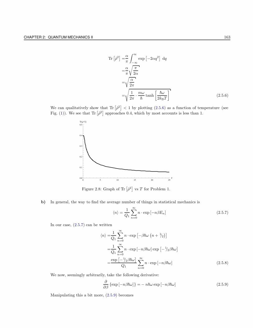
CHAPTER 2: QUANTUM MECHANICS II 163
Tr[ρ2]
=α
π
∫ ∞
−∞exp
[−2αq2
]dq
=α
π
√π
2α
=
√α
2π
=
√1
2π· mω
~tanh
[~ω
2kBT
](2.5.6)
We can qualitatively show that Tr[ρ2]< 1 by plotting (2.5.6) as a function of temperature (see
Fig. (1)). We see that Tr[ρ2]
approaches 0.4, which by most accounts is less than 1.
0 5 10 15 20 25T0.0
0.1
0.2
0.3
0.4
0.5
Tr@Ρ^2D
Figure 2.8: Graph of Tr[ρ2]
vs T for Problem 1.
b) In general, the way to find the average number of things in statistical mechanics is
〈n〉 =1
Q1
∞∑
n=0
n · exp [−nβEn] (2.5.7)
In our case, (2.5.7) can be written
〈n〉 =1
Q1
∞∑
n=0
n · exp[−β~ω
(n+ 1/2
)]
=1
Q1
∞∑
n=0
n · exp [−nβ~ω] exp[−1/2β~ω
]
=exp
[−1/2β~ω
]
Q1
∞∑
n=0
n · exp [−nβ~ω] (2.5.8)
We now, seemingly arbitrarily, take the following derivative:
∂
∂βexp [−nβ~ω] = − n~ω exp [−nβ~ω] (2.5.9)
Manipulating this a bit more, (2.5.9) becomes
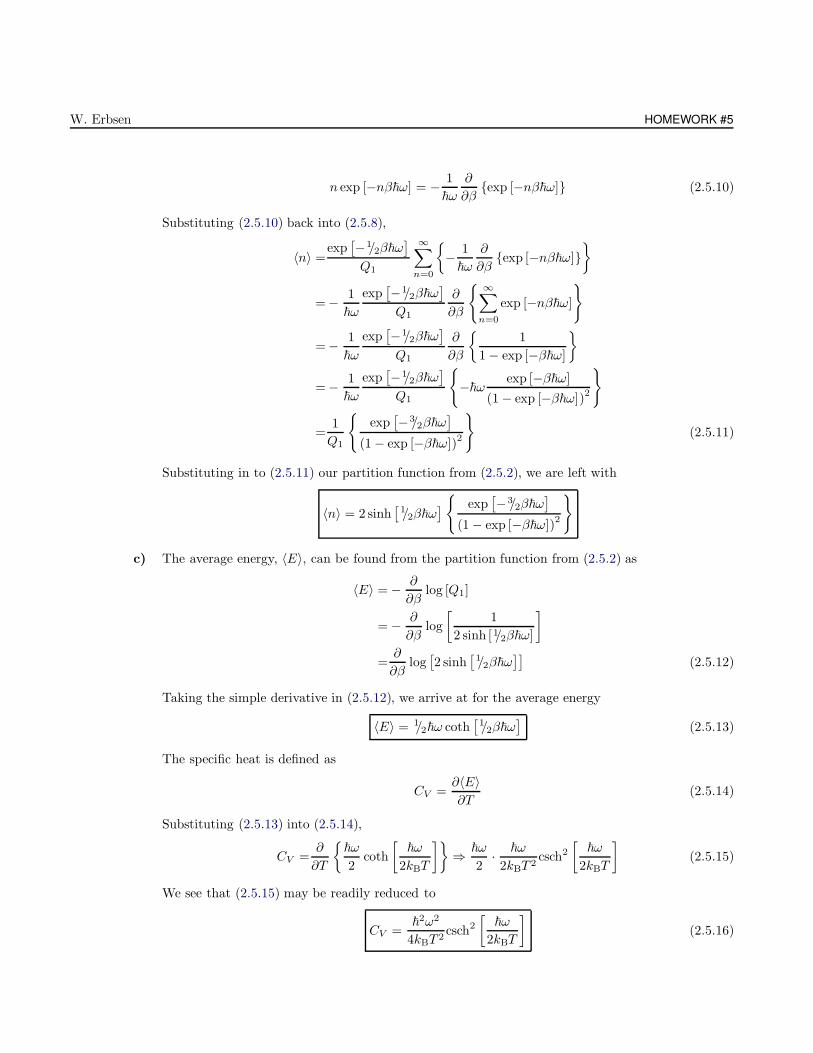
W. Erbsen HOMEWORK #5
n exp [−nβ~ω] = − 1
~ω
∂
∂βexp [−nβ~ω] (2.5.10)
Substituting (2.5.10) back into (2.5.8),
〈n〉 =exp
[−1/2β~ω
]
Q1
∞∑
n=0
− 1
~ω
∂
∂βexp [−nβ~ω]
= − 1
~ω
exp[−1/2β~ω
]
Q1
∂
∂β
∞∑
n=0
exp [−nβ~ω]
= − 1
~ω
exp[−1/2β~ω
]
Q1
∂
∂β
1
1 − exp [−β~ω]
= − 1
~ω
exp[−1/2β~ω
]
Q1
−~ω
exp [−β~ω]
(1 − exp [−β~ω])2
=1
Q1
exp
[−3/2β~ω
]
(1 − exp [−β~ω])2
(2.5.11)
Substituting in to (2.5.11) our partition function from (2.5.2), we are left with
〈n〉 = 2 sinh[1/2β~ω
]
exp[−3/2β~ω
]
(1 − exp [−β~ω])2
c) The average energy, 〈E〉, can be found from the partition function from (2.5.2) as
〈E〉 = − ∂
∂βlog [Q1]
= − ∂
∂βlog
[1
2 sinh [1/2β~ω]
]
=∂
∂βlog[2 sinh
[1/2β~ω
]](2.5.12)
Taking the simple derivative in (2.5.12), we arrive at for the average energy
〈E〉 = 1/2~ω coth[1/2β~ω
](2.5.13)
The specific heat is defined as
CV =∂〈E〉∂T
(2.5.14)
Substituting (2.5.13) into (2.5.14),
CV =∂
∂T
~ω
2coth
[~ω
2kBT
]⇒ ~ω
2· ~ω
2kBT 2csch2
[~ω
2kBT
](2.5.15)
We see that (2.5.15) may be readily reduced to
CV =~2ω2
4kBT 2csch2
[~ω
2kBT
](2.5.16)
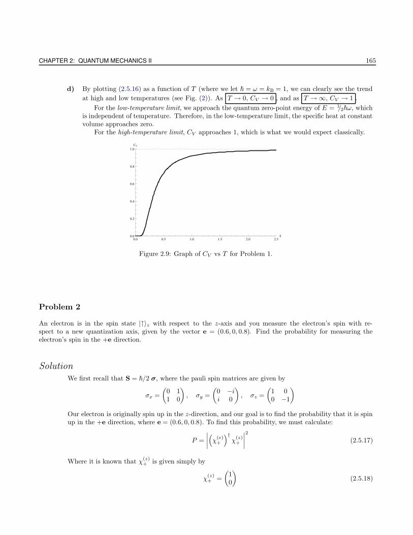
CHAPTER 2: QUANTUM MECHANICS II 165
d) By plotting (2.5.16) as a function of T (where we let ~ = ω = kB = 1, we can clearly see the trend
at high and low temperatures (see Fig. (2)). As T → 0, CV → 0 , and as T → ∞, CV → 1 .
For the low-temperature limit, we approach the quantum zero-point energy of E = 1/2~ω, whichis independent of temperature. Therefore, in the low-temperature limit, the specific heat at constantvolume approaches zero.
For the high-temperature limit, CV approaches 1, which is what we would expect classically.
0.0 0.5 1.0 1.5 2.0 2.5T0.0
0.2
0.4
0.6
0.8
1.0
CV
Figure 2.9: Graph of CV vs T for Problem 1.
Problem 2
An electron is in the spin state |↑〉z with respect to the z-axis and you measure the electron’s spin with re-spect to a new quantization axis, given by the vector e = (0.6, 0, 0.8). Find the probability for measuring theelectron’s spin in the +e direction.
Solution
We first recall that S = ~/2 σ, where the pauli spin matrices are given by
σx =
(0 11 0
), σy =
(0 −ii 0
), σz =
(1 00 −1
)
Our electron is originally spin up in the z-direction, and our goal is to find the probability that it is spinup in the +e direction, where e = (0.6, 0, 0.8). To find this probability, we must calculate:
P =
∣∣∣∣(χ
(e)+
)†χ
(z)+
∣∣∣∣2
(2.5.17)
Where it is known that χ(z)+ is given simply by
χ(z)+ =
(10
)(2.5.18)
W. Erbsen HOMEWORK #5
In order to find χ(e)+ , we must diagonalize the spin matrix Se. We do that by taking the normal component
with S:
Se =e · S
=0.6Sx + 0.8Sz
=~
2
0.6
(0 11 0
)+ 0.8
(1 00 −1
)
=~
2
(0 0.6
0.6 0
)+
(0.8 00 −0.8
)
=~
2
(0.8 0.60.6 −0.8
)(2.5.19)
To find the eigenvalues and eigenvectors of (2.5.19), we take the determinate of the matrix and set it tozero:
~
2
∣∣∣∣0.8− λ 0.6
0.6 −0.8 − λ
∣∣∣∣ = 0 −→ (0.8− λ) (−0.8 − λ) − (0.6) (0.6) = 0
−→− 0.64− 0.8λ+ 0.8λ+ λ2 − 0.36 = 0
−→λ = ±1
To find the eigenvector corresponding to λ = +1,
~
2
(0.8− 1 0.6
0.6 −0.8 − 1
)⇒ ~
2
(−0.2 0.60.6 −1.8
)(2.5.20)
To find the eigenvectors,
~
2
(−0.2 0.60.6 −1.8
)(αβ
)=
(00
)−→ −0.2α+ 0.6β = 0
0.6α− 1.8β = 0
For the first line, we can let α = −0.6, and β = 0.2. Accordingly, our eigenspinor becomes
χ(e)+ =
(−0.3
0.1
)(2.5.21)
We can now substitute (2.5.21) and (2.5.18) back into (2.5.17) to find the probability,
P =
∣∣∣∣∣
(−0.3
0.1
)†(10
)∣∣∣∣∣
2
⇒∣∣∣∣(−0.3 0.1
)(10
)∣∣∣∣2
⇒ |−0.3|2 −→ P = 0.09 (2.5.22)
Part II
CHAPTER 2: QUANTUM MECHANICS II 167
Exercise 15.25
If an ensemble E consists of an equal-probability mixture of two nonorthogonal (but normalized) states |Ψ1〉and |Ψ2〉 with overlap C = 〈Ψ1|Ψ2〉, evaluate the Shannon mixing entropy H(E ) and the von Neumann entropy,S(ρ). Compare the latter with the former as |C| varies between 0 and 1. What happens as C → 0?
Solution
The Shannon mixing entropy is given by (15.126):
H(E ) = −N∑
i=1
pi log [pi] (2.5.23)
And the density operator is given by
ρ =
N∑
i=1
piρi ⇒N∑
i=1
pi|Ψi〉〈Ψi|
And since the states have equal probabilities,
p1 = p2 =1
2
Substituting this into (2.5.23) we have
H(E ) = −2∑
i=1
pi log [pi] = −2∑
i=1
log[1/2]
2= log [2] = 0.693147... (2.5.24)
The Von Neumann entropy is defined by (15.128):
S(ρ) = −n∑
i=1
pi log [pi] ⇒ −n∑
i=1
〈pi|ρ log [ρ] |pi〉 ⇒ −Tr(ρ log [ρ]) (2.5.25)
Where p1,2 is given in Exercise 15.24. So,
p1,2 =1 ±
√|〈Ψ1|Ψ2〉|2
2⇒ 1 ± C
2
−→ p1 =1 +C
2, p2 =
1 −C
2
Putting this back into (2.5.25), we have
S(ρ) = −(
1 + C
2
)log
[1 + C
2
]−(
1 −C
2
)log
[1 −C
2
](2.5.26)
For the functional dependence of S(ρ) on C please see Fig. (3). As we can see, when C = 0 thenS(ρ) = log [2] = H(E ), however as C is increased S(ρ) decreases. Explicitly, as C → 0, we have
S(ρ) = log [2]
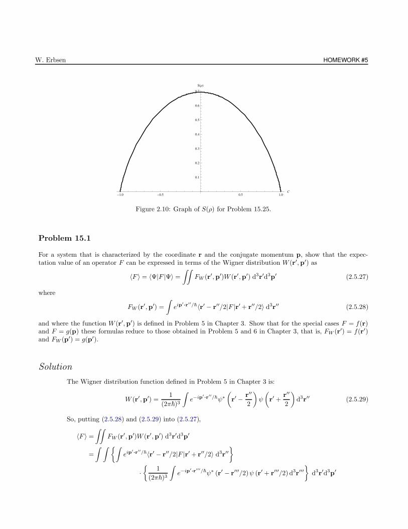
W. Erbsen HOMEWORK #5
-1.0 -0.5 0.5 1.0C
0.1
0.2
0.3
0.4
0.5
0.6
0.7
SHΡL
Figure 2.10: Graph of S(ρ) for Problem 15.25.
Problem 15.1
For a system that is characterized by the coordinate r and the conjugate momentum p, show that the expec-tation value of an operator F can be expressed in terms of the Wigner distribution W (r′,p′) as
〈F 〉 = 〈Ψ|F |Ψ〉 =
∫∫FW (r′,p′)W (r′,p′) d3r′d3p′ (2.5.27)
where
FW (r′,p′) =
∫eip′
·r′′/~〈r′ − r′′/2|F |r′ + r′′/2〉 d3r′′ (2.5.28)
and where the function W (r′,p′) is defined in Problem 5 in Chapter 3. Show that for the special cases F = f(r)and F = g(p) these formulas reduce to those obtained in Problem 5 and 6 in Chapter 3, that is, FW (r′) = f(r′)and FW (p′) = g(p′).
Solution
The Wigner distribution function defined in Problem 5 in Chapter 3 is:
W (r′,p′) =1
(2π~)3
∫e−ip′
·r′′/~ψ∗(r′ − r′′
2
)ψ
(r′ +
r′′
2
)d3r′′ (2.5.29)
So, putting (2.5.28) and (2.5.29) into (2.5.27),
〈F 〉 =
∫∫FW (r′,p′)W (r′,p′) d3r′d3p′
=
∫ ∫ ∫eip′
·r′′/~〈r′ − r′′/2|F |r′ + r′′/2〉 d3r′′
·
1
(2π~)3
∫e−ip′
·r′′′/~ψ∗ (r′ − r′′′/2)ψ (r′ + r′′′/2) d3r′′′
d3r′d3p′
CHAPTER 2: QUANTUM MECHANICS II 169
=1
(2π~)3
∫∫ ∫∫eip′
·(r′′−r′′′)/~〈r′ − r′′/2|F |r′ + r′′/2〉
· ψ∗ (r′ − r′′′/2)ψ (r′ + r′′′/2) d3r′′′d3r′′
d3r′d3p′ (2.5.30)
We recognize that r′′′ integral collapses when looking at the exponent, which reduces to the delta functionδ (r′′ − r′′′). So, (2.5.30) becomes
〈F 〉 =1
(2π~)3
∫∫〈r′ − r′′/2|F |r′ + r′′/2〉ψ∗ (r′ − r′′/2)ψ (r′ + r′′2) d3r′′d3r′ (2.5.31)
We also recall from Chapter 17 that the Wigner Exckart Theorem holds if the determinate of J = 1,where J is
J =
∂
∂r′
(r′ − r′′
2
)∂
∂r′′
(r′ − r′′
2
)
∂
∂r′
(r′ +
r′′
2
)∂
∂r′′
(r′ +
r′′
2
)
⇒
(1 −1/2
1 1/2
)
Taking the determinate of J,
Det J =
∣∣∣∣∣1 −1/2
1 1/2
∣∣∣∣∣⇒ (1)(1/2) − (−1/2)(1) ⇒ 1 X (2.5.32)
We can define two quantities r1 and r2 as
r1 =r′ − r′′
2
r2 =r′ +r′′
2
Using these, we can then rewrite (2.5.31) as
〈F 〉 =
∫∫〈r1|F |r2〉ψ∗ (r1)ψ (r2) d3r1d
3r2
=
∫∫〈r1|F |r2〉〈r1|r2〉 d3r1d
3r2
=
∫∫〈r1|F |r2〉δ (r1 − r2) d3r1d
3r2
=〈F 〉 (2.5.33)
Using the results from (2.5.32) and also the results from (2.5.33), we can therefore safely make the
conclusion that 〈F 〉 can be expressed in terms of W (r′,p′) as in (2.5.27).
The next parts of this problem ask us to show that FW (r′) = f(r′) and FW (p′) = g(p′). Startingwith FW (r′), we rewrite (2.5.28) as
FW (r′,p′) =
∫eip′
·r′′/~〈r′ − r′′/2|f(r)|r′ + r′′/2〉 d3r′′
=
∫eip′
·r′′/~f(r)〈r′ − r′′/2|r′ + r′′/2〉 d3r′′
W. Erbsen HOMEWORK #5
=
∫eip′
·r′′/~f(r)δ (r′ − r′′/2 − (r′ + r′′/2)) d3r′′
=
∫eip′
·r′′/~f(r)δ (r′′) d3r′′ (2.5.34)
From (2.5.34) we can safely conclude that FW (r′,p′) = f(r′). To do the same for FW (p′), we proceed
in very much the same way, except we expand g(p′) in p eigenstates:
FW (r′,p′) =
∫eip′
·r′′/~〈r′ − r′′/2|g(p′)
∫|p〉〈p| d3p
|r′ + r′′/2〉 d3r′′
=
∫∫eip′
·r′′/~g(p′)〈r′ − r′′/2|p〉〈p|r′ + r′′/2〉 d3r′′d3p (2.5.35)
Recalling from a previous homework set that
〈r|p〉 =1
(2π~)3/2eir·p/~ (2.5.36)
Rewriting (2.5.35), and applying (2.5.36),
FW (r′,p′) =
∫∫eip′
·r′′/~g(p′)〈r′ − r′′/2|p〉 (〈r′ + r′′/2|p〉)∗ d3r′′d3p
=
∫∫eip′
·r′′/~g(p′)
1
(2π~)3/2ei(r′−r′′/2)·p/~
1
(2π~)3/2e−i(r′+r′′/2)·p/~
d3r′′d3p
=
∫∫eip′
·r′′/~g(p′)
1
(2π~)3/2ei(r′−r′′/2)·p/~
1
(2π~)3/2e−i(r′+r′′/2)·p/~
d3r′′d3p
=1
(2π~)3
∫∫eip′
·r′′/~g(p′)ei(r′−r′′/2)·p/~e−i(r′+r′′/2)·p/~ d3r′′d3p
=1
(2π~)3
∫∫g(p′)ei(p′−p)·r′′/~ d3r′′d3p (2.5.37)
It is easy to see that the exponential term in (2.5.37) collapses to a δ-function, and we are left with
nothing other than FW (r′,p′) = g(p′).
Exercise 16.8
Prove that the only matrix which commutes with all three Pauli matrices is a multiple of the identity. Alsoshow that no matrix exists which anti-commutes with all three Pauli matrices.
Solution
Imagining some matrix A:
CHAPTER 2: QUANTUM MECHANICS II 171
A =
(a bc d
)
To answer the first part of the question, we look to evaluate:
[A,σ] = [A, σx] + [A, σy] + [A, σz] = 0 (2.5.38)
The first commutator is given by
[A, σx] =Aσx − σxA
=
(a bc d
)(0 11 0
)−(a bc d
)(0 11 0
)
=
(b ad c
)−(c da b
)(2.5.39)
While the second is
[A, σy] =i
(b −ad −c
)− i
(−c −da b
)(2.5.40)
And finally, the third commutator is
[A, σz] =
(a −bc −d
)−(a b−c −d
)(2.5.41)
Plugging (2.5.39)-(2.5.41) back into (2.5.38),
[A,σ] =
(b ad c
)−(c da b
)+ i
(b −ad −c
)− i
(−c −da b
)+
(a −bc −d
)−(a b−c −d
)
=
(b ad c
)+ i
(b −ad −c
)−(c da b
)+ i
(−c −da b
)+
(a −bc −d
)−(a b−c −d
)
=
(b+ ib+ c − ic a− d− 2b
d+ id− (a + ia) + 2c c− ic − (b+ ib)
)(2.5.42)
This leaves us with four equations and four unknowns:
b(1 + i) + c(1 − i) = 0 (2.5.43a)
a− 2b− d = 0 (2.5.43b)
d(1 + i) − a(1 + i) + 2c = 0 (2.5.43c)
c(1 − i) − b(1 + i) = 0 (2.5.43d)
Solving (2.5.43a) for b(1 + i), our four equations become
b(1 + i) = −c(1 − i) (2.5.44a)
a+ 2c(1− i)
(1 + i)− d = 0 (2.5.44b)
d(1 + i) − a(1 + i) + 2c = 0 (2.5.44c)
W. Erbsen HOMEWORK #5
c(1 − i) + c(1 − i) = 0 −→ c = 0 (2.5.44d)
Now that we know that we require that c = 0, (2.5.44a)-(2.5.44c) become
b(1 + i) = 0 −→ b = 0 (2.5.45a)
a− d = 0 −→ a = d (2.5.45b)
d(1 + i) − a(1 + i) = 0 (2.5.45c)
From (2.5.44d), (2.5.45a) and (2.5.45b), it is clear that b = c = 0 and a = d. Therefore, we can now say
that the only matrix which commutes with all three Pauli matrices is a multiple of the identity. We note
that multiplying the commutator by a constant will not change this.The next part of the question asks us to show that no matrix exists which anti-commutes with all
three Pauli matrices. To show this, we proceed in the same way we did in the last problem:
[A, σx] =
(b ad c
)−(c da b
)6= 0 (2.5.46)
[A, σy] =i
(b −ad −c
)− i
(−c −da b
)6= 0 (2.5.47)
[A, σz] =
(a −bc −d
)−(a b−c −d
)6= 0 (2.5.48)
Following the same logic as before, we can see that the anti-commutation condition will only exist if
a = b = c = d = 0, so therefore no matrix exists which anti-commutes with all three Pauli matrices.
Exercise 16.15
In many applications, conservation laws and selection rules cause a decaying two-level system to be preparedin an eigenstate of σz, say
(10
), and governed by the simple normal Hamiltonian matrix
H = a1 + bσx (2.5.49)
where a and b are generally complex constants. In terms of the energy difference ∆E = E02 −E01 and the decayrates Γ1 and Γ2, calculate the probabilities of finding the system at time t in state α or state β, respectively.
Solution
We first recall that from the prompt, we have α =(10
), and according to (2.5.49),
H =a
(1 00 1
)+ b
(0 11 0
)
=
(a 00 a
)+
(0 bb 0
)
=
(a bb a
)(2.5.50)
CHAPTER 2: QUANTUM MECHANICS II 173
We also note that from the prompt that ∆E = E02 −E01, and we recall from (16.81) from Merzbacher,
E1 =E01 − iΓ1
2(2.5.51a)
E2 =E02 − iΓ2
2(2.5.51b)
Taking the difference of (2.5.51a) and (2.5.51b),
E2 −E1 =E02 − iΓ2
2−E01 − i
Γ1
2
=∆E − i∆Γ
2(2.5.52)
Where ∆Γ = Γ2 − Γ1. We also recall from (16.83),
〈β|T (t, 0)|α〉 =〈β|H|α〉E2 −E1
(exp
[− iE2t
~
]− exp
[− iE1t
~
])(2.5.53)
We already know what 〈β|H|α〉 is:
〈β|H|α〉 =β†(a bb a
)α
=(0 1
)(a bb a
)(10
)
=b (2.5.54)
Substituting (2.5.52) and (2.5.54) into (2.5.53),
〈β|T (t, 0)|α〉 =b
∆E − i/2∆Γ
exp
[− i(E02 − i/2Γ2
)t
~
]− exp
[− i(E01 − i/2Γ1
)t
~
](2.5.55)
Taking the modulus squared of (2.5.56),
Pα→β = |〈β|T (t, 0)|α〉|2
=|b|2
|∆E − i/2∆Γ|2
∣∣∣∣∣exp
[− i(E02 − i/2Γ2
)t
~
]− exp
[− i(E01 − i/2Γ1
)t
~
]∣∣∣∣∣
2
=|b|2
(∆E)2 − 1/4 (∆Γ)2
∣∣∣∣∣exp
[− i(E02 − i/2Γ2
)t
~
]− exp
[− i(E01 − i/2Γ1
)t
~
]∣∣∣∣∣
2 (2.5.56)
The bracketed term in (2.5.56) can be reduced to
... =
(exp
[i(E02 + i/2Γ2
)t
~
]− exp
[i(E01 + i/2Γ1
)t
~
])(exp
[− i(E02 − i/2Γ2
)t
~
]
− exp
[− i(E01 − i/2Γ1
)t
~
])
W. Erbsen HOMEWORK #6
=exp
[−Γ2
~
]− exp
[−(2i∆E − (Γ1 + Γ2)) t
2~
]− exp
[(2i∆E − (Γ1 + Γ2)) t
2~
]+ exp
[−Γ1
~
]
(2.5.57)
Substituting (2.5.57) into (2.5.56),
Pα→β =|b|2
(∆E)2 − 1/4 (∆Γ)
2
exp
[−Γ2
~
]− exp
[−(2i∆E − (Γ1 + Γ2)) t
2~
]
− exp
[(2i∆E − (Γ1 + Γ2)) t
2~
]+ exp
[−Γ1
~
]
To find Pα→α, the only difference is that 〈α|H|α〉 = a, and so we have
Pα→α =|a|2
(∆E)2 − 1/4 (∆Γ)
2
exp
[−Γ2
~
]− exp
[−(2i∆E − (Γ1 + Γ2)) t
2~
]
− exp
[(2i∆E − (Γ1 + Γ2)) t
2~
]+ exp
[−Γ1
~
]
2.6 Homework #6
Exercise 16.23
If a constant magnetic field B0, pointing along the z-axis, and a field B1, rotating with angular velocity ω inthe xy-plane, act in concert on a spin system (gyromagnetic ratio γ), calculate the polarization vector P as afunction of time. Assume P to point in the z-direction at t = 0. Calculate the Rabi oscillations in the rotatingframe, and plot the average probability that the particle has “spin down” as a function of ω/ω0 for a value ofB1/B0 = 0.1. Show that a resonance occurs when ω = −γB0 . (This arrangement is a model for all magneticresonance experiments.)
Solution
The processing magnetic field, B1, can be expressed in terms of its angular frequency ω and the time tas
B1 = B1 cos (ωt) i∓ B1 sin (ωt) j (2.6.1)
The sign in (2.6.1) determines the direction of rotation. Let’s let it be rotating clockwise, so that ∓ → −.Furthermore, we are told that the static field points purely in the z-direction, so that B0 = (0, 0, B0).The total magnetic field is of course
B = B1 + B0 ⇒ B = B1 cos (ωt) i −B1 sin (ωt) j + B0 k (2.6.2)

CHAPTER 2: QUANTUM MECHANICS II 175
We now set our minds to finding the Hamiltonian matrix, H, which describes our system. We now recallthat in general, the Hamiltonian for a particle with magnetic moment µ in some magnetic field B isgiven by H = −µ · B, where H is a matrix. For the case of a spin in a magnetic field, the magneticmoment becomes µ = −γ~σ/2, where σ denotes the respective Pauli spin matrix.
Accordingly, the Hamiltonian matrix becomes
H = − γ~
2
[B1 cos (ωt)σx i −B1 sin (ωt) σy j +B0σz k
](2.6.3)
We can rewrite (2.6.3) by replacing our trig functions with exponentials:
H = − γ~
2
[B1
2
(eiωt + e−iωt
)σx i− B1
2i
(eiωt − e−iωt
)σy j +B0σz k
]
= − γ~
2
[B1
2
(eiωt + e−iωt
)σx i− 1
i
(eiωt − e−iωt
)σy j
+B0σz k
](2.6.4)
We also recall that the Pauli spin matrices are
σx =
(0 11 0
), σy = i
(0 −11 0
), σz =
(1 00 −1
)
Substituting in σx, σy and σz into (2.6.4),
H = − γ~
2
[B1
2
(eiωt + e−iωt
)(0 11 0
)− 1
i
(eiωt − e−iωt
)i
(0 −11 0
)+B0
(1 00 −1
)]
= − γ~
2
[B1
2
(eiωt + e−iωt
)(0 11 0
)−(eiωt − e−iωt
)(0 −11 0
)+B0
(1 00 −1
)](2.6.5)
We can combine the first two terms in (2.6.5) as(
0 eiωt + e−iωt
eiωt + e−iωt 0
)−(
0 −(eiωt − e−iωt
)
eiωt − e−iωt 0
)= 2
(0 eiωt
e−iωt 0
)
Using this, (2.6.5) becomes
H = − γ~
2
[B1
(0 eiωt
e−iωt 0
)+B0
(1 00 −1
)](2.6.6)
We now define the following quantities
ω0 =γB0
2, ω1 =
γB1
2
Accordingly, (2.6.6) becomes
H = − ~ω1
(0 eiωt
e−iωt 0
)− ~ω0
(1 00 −1
)(2.6.7)
At this point, we define the following time-dependent wave function
χ(t) =
(c1(t)c2(t)
)(2.6.8)
W. Erbsen HOMEWORK #6
Whose first derivative with respect to time is of course
d
dtχ(t) =
(c1(t)c2(t)
)(2.6.9)
We now require that our Hamiltonian and associated wave functions satisfy the TDSE as
i~d
dtχ(t) = Hχ(t) (2.6.10)
Substituting (2.6.7)-(2.6.9) into (2.6.10) yields
i~
(c1(t)c2(t)
)=
−~ω1
(0 eiωt
e−iωt 0
)− ~ω0
(1 00 −1
)·
(c1(t)c2(t)
)
i
(c1(t)c2(t)
)= − ω1
(c2(t)e
iωt
c1(t)e−iωt
)− ω0
(c1(t)−c2(t)
)
(c1(t)c2(t)
)=iω1
(c2(t)e
iωt
c1(t)e−iωt
)+ iω0
(c1(t)−c2(t)
)(2.6.11)
It is easy to see that (2.6.11) yields two coupled differential equations,
c1(t) =iω1c2(t)eiωt + iω0c1(t) (2.6.12a)
c2(t) =iω1c1(t)e−iωt − iω0c2(t) (2.6.12b)
The two equations (2.6.12a) and (2.6.12b) constitute a set of coupled differential equations. The moststraightforward way to solve these coupled equations is to evaluate the derivative of one of the equationsand then plug in the other one. This was done via Mathematica, including the initial conditions. Theresult is
c1(t) =[cos (ω′t/2) + i/ω′
(ω0 − 1/2ω
)sin (ω′t/2)
]eiωt/2 (2.6.13a)
c2(t) =
[i/ω′
√(ω′)2 − (1/2ω − ω0)
2sin (ω′t/2)
]e−iωt/2 (2.6.13b)
Where I have defined ω′ =√
(1/2ω − ω0)2
+ ω21 . We can further simplify (2.6.13a) and (2.6.13b) by
letting
α =
√(ω′)2 − (1/2ω − ω0)
2
ω′ , β =ω′t
2, γ =
ω0 − ω
ω′ , δ =ωt
2(2.6.14)
Using α, β and γ, we can now rewrite (2.6.13a) and (2.6.13b) as
c1(t) = [cos (β) + iγ sin (β)] eiδ (2.6.15a)
c2(t) =iα sin (β) e−iδ (2.6.15b)
We recall that the Pauli spin matrices from before, and to find the polarization vector P as a functionof time, we must find each component by taking the inner product of the respective spin matrix. Forinstance, we can find Px as follows:
Px =〈χ(t)|σx|χ(t)〉
CHAPTER 2: QUANTUM MECHANICS II 177
=χ†(t)σxχ(t)
=(c∗1(t) c∗2(t)
)(0 11 0
)(c1(t)c2(t)
)
=(c∗2(t) c∗1(t)
)(c1(t)c2(t)
)
=c∗2(t)c1(t) + c∗1(t)c2(t) (2.6.16)
Substituting in to (2.6.16) the results from (2.6.15a) and (2.6.15b),
Px =(iα sin (β) e−iδ
)∗ [(cos (β) + iγ sin (β)) eiδ
]+[(cos (β) + iγ sin (β)) eiδ
]∗ (iα sin (β) e−iδ
)
= − iα sin (β) eiδ (cos (β) + iγ sin (β)) eiδ + iα (cos (β) − iγ sin (β)) e−iδ sin (β) e−iδ
=iα− sin (β) cos (β) e2iδ − iγ sin2 (β) e2iδ + sin (β) cos (β) e−2iδ − iγ sin2 (β) e−2iδ
=iα− sin (β) cos (β)
[e2iδ − e−2iδ
]− iγ sin2 (β)
[e2iδ + e−2iδ
]
=iα− sin (β) cos (β) [2i sin (2δ)] − iγ sin2 (β) [2 cos (2δ)]
=2α sin (β) cos (β) sin (2δ) + 2αγ sin2 (β) cos (2δ)
=2α sin (β) [cos (β) sin (2δ) + sin (β) cos (2δ)] (2.6.17)
Similarly, we can find Py in the following way:
Py =〈χ(t)|σy|χ(t)〉=χ†(t)σyχ(t)
=(c∗1(t) c∗2(t)
)(0 −ii 0
)(c1(t)c2(t)
)
=(ic∗2(t) −ic∗1(t)
)(c1(t)c2(t)
)
=ic∗2(t)c1(t) − ic∗1(t)c2(t) (2.6.18)
Substituting in the appropriate values,
Py =i(iα sin (β) e−iδ
)∗ [(cos (β) + iγ sin (β) eiδ
)]− i[(cos (β) + iγ sin (β)) eiδ
]∗ (iα sin (β) e−iδ
)
= − α sin (β) eiδ (cos (β) + iγ sin (β)) eiδ + α (cos (β) − iδ sin (β)) e−iδ sin (β) e−iδ
=α sin (β)(cos (β) + iγ sin (β)) e2iδ + (cos (β) − iγ sin (β)) e−2iδ
=α sin (β)cos (β) e2iδ + iγ sin (β) e2iδ + cos (β) e−2iδ − iγ sin (β) e−2iδ
=α sin (β)cos (β)
[e2iδ + e−2iδ
]+ iγ sin (β)
[e2iδ − e−2iδ
]
=α sin (β) cos (β) [2 cos (2δ)] + iδ sin (β) [2i sin (2δ)]=2α sin (β) cos (β) cos (2δ) − γ sin (β) sin (2δ) (2.6.19)
And finally, for Pz we have
Pz =〈χ(t)|σz|χ(t)〉=χ†(t)σzχ(t)
=(c∗1(t) c∗2(t)
)(1 00 −1
)(c1(t)c2(t)
)
W. Erbsen HOMEWORK #6
=(c∗1(t) −c∗2(t)
)(c1(t)c2(t)
)
=c∗1(t)c1(t) − c∗2(t)c2(t) (2.6.20)
With the coefficients, (2.6.20) turns in to
Pz =[(cos (β) + iγ sin (β)) eiδ
]∗ [(cos (β) + iγ sin (β)) eiδ
]−(iα sin (β) e−iδ
)∗ (iα sin (β) e−iδ
)
=(cos (β) − iγ sin (β)) (cos (β) + iγ sin (β)) + α2 sin2 (β)
= cos2 (β) + γ2 sin2 (β) + α2 sin2 (β)
= cos2 (β) + sin2 (β)(α2 + γ2
)(2.6.21)
So, the polarization vector, P, is given by (2.6.17), (2.6.19) and (2.6.21) as
Px = 2α sin (β) [cos (β) sin (2δ) + sin (β) cos (2δ)]Py = 2α sin (β) cos (β) cos (2δ) − γ sin (β) sin (2δ)Pz = cos2 (β) + sin2 (β)
(α2 + γ2
)
Where α, β, γ and δ are defined by (2.6.14). To find the probability that the spin polarization is up asa function of time, we evaluate
P↑(t) =∣∣∣〈χ(z)
+ |χ(t)〉∣∣∣2
⇒∣∣∣∣(1 0
)(c1(t)c2(t)
)∣∣∣∣2
⇒ |c1(t)|2 ⇒ c∗1(t)c1(t) (2.6.22)
And now we have
P↑(t) = [cos (β) + iγ sin (β)]∗[cos (β) + iγ sin (β)] −→ P↑(t) = cos2 (β) + γ2 sin2 (β) (2.6.23)
And similarly,
P↓(t) =∣∣∣〈χ(z)
− |χ(t)〉∣∣∣2
⇒∣∣∣∣(0 1
)(c1(t)c2(t)
)∣∣∣∣2
⇒ |c2(t)|2 ⇒ c∗2(t)c2(t) (2.6.24)
And now
P↓(t) = (iα sin (β))∗(iα sin (β)) −→ P↓(t) = α2 sin2 (β) (2.6.25)
Resonance occurs when the probability from (2.6.25) equals 1. To evaluate the condition, we rewrite(2.6.25) by substituting back in the values of α and β from (2.6.14):
P↓(t) =(ω1)
2
(1/2ω − ω0)2 + (ω1)
2sin2
√(1/2ω − ω0)
2 + (ω1)2
2t
(2.6.26)
The maximum value of the sin2 (...) term is 1, so we are left with:
(ω1)2
(1/2ω − ω0)2
+ (ω1)2 = 1 −→
(1/2ω − ω0
)2= 0 −→ ω = 2ω0 (2.6.27)
Using (2.6.27) and our previous definition of ω0, we find that
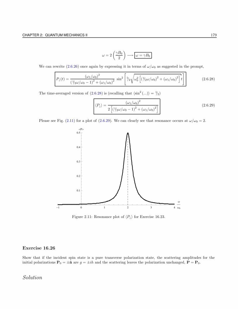
CHAPTER 2: QUANTUM MECHANICS II 179
ω = 2
(γB0
2
)−→ ω = γB0
We can rewrite (2.6.26) once again by expressing it in terms of ω/ω0 as suggested in the prompt,
P↓(t) =(ω1/ω0)
2
(1/2ω/ω0 − 1)2
+ (ω1/ω0)2 sin2
[1/2
√ω2
0
[(1/2ω/ω0)
2+ (ω1/ω0)
2]t
](2.6.28)
The time-averaged version of (2.6.28) is (recalling that 〈sin2 (...)〉 = 1/2)
〈P↓〉 =(ω1/ω0)
2
2[(1/2ω/ω0 − 1)
2+ (ω1/ω0)
2] (2.6.29)
Please see Fig. (2.11) for a plot of (2.6.29). We can clearly see that resonance occurs at ω/ω0 = 2.
-1 0 1 2 3 4
Ω
Ω0
0.1
0.2
0.3
0.4
0.5
<P>
Figure 2.11: Resonance plot of 〈P↓〉 for Exercise 16.23.
Exercise 16.26
Show that if the incident spin state is a pure transverse polarization state, the scattering amplitudes for theinitial polarizations P0 = ±n are g = ±ih and the scattering leaves the polarization unchanged, P = P0.
Solution
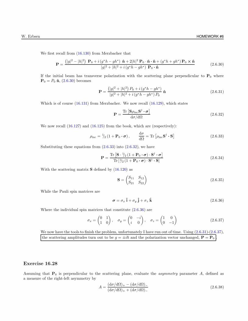
W. Erbsen HOMEWORK #6
We first recall from (16.130) from Merzbacher that
P =
(|g|2 − |h|2
)P0 + i (g∗h− gh∗) n + 2|h|2 P0 · n · n + (g∗h + gh∗)P0 × n
|g|2 + |h|2 + i (g∗h− gh∗) P0 · n(2.6.30)
If the initial beam has transverse polarization with the scattering plane perpendicular to P0 whereP0 = P0 n, (2.6.30) becomes
P =
(|g|2 + |h|2
)P0 + i (g∗h− gh∗)
|g|2 + |h|2 + i (g∗h− gh∗)P0n (2.6.31)
Which is of course (16.131) from Merzbacher. We now recall (16.129), which states
P =Tr[SρincS
†· σ]
dσ/dΩ(2.6.32)
We now recall (16.127) and (16.125) from the book, which are (respectively):
ρinc = 1/2 (1 + P0 · σ) ,dσ
dΩ= Tr
[ρincS
†· S]
(2.6.33)
Substituting these equations from (2.6.33) into (2.6.32), we have
P =Tr[S · 1/2 (1 + P0 · σ) · S†
· σ]
Tr [1/2 (1 + P0 · σ) · S† · S](2.6.34)
With the scattering matrix S defined by (16.120) as
S =
(S11 S12
S21 S22
)(2.6.35)
While the Pauli spin matrices are
σ = σx i + σy j + σz k (2.6.36)
Where the individual spin matrices that constitute (2.6.36) are
σx =
(0 11 0
), σy =
(0 −ii 0
), σz =
(1 00 −1
)(2.6.37)
We now have the tools to finish the problem, unfortunately I have run out of time. Using (2.6.31)-(2.6.37),
the scattering amplitudes turn out to be g = ±i~ and the polarization vector unchanged, P = P0 .
Exercise 16.28
Assuming that P0 is perpendicular to the scattering plane, evaluate the asymmetry parameter A, defined asa measure of the right-left asymmetry by
A =(dσ/dΩ)+ − (dσ/dΩ)−(dσ/dΩ)+ + (dσ/dΩ)−
(2.6.38)
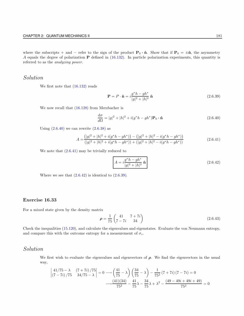
CHAPTER 2: QUANTUM MECHANICS II 181
where the subscripts + and − refer to the sign of the product P0 · n. Show that if P0 = ±n, the asymmetryA equals the degree of polarization P defined in (16.132). In particle polarization experiments, this quantity isreferred to as the analyzing power.
Solution
We first note that (16.132) reads
P = P · n = ig∗h− gh∗
|g|2 + |h|2 n (2.6.39)
We now recall that (16.128) from Merzbacher is
dσ
dΩ= |g|2 + |h|2 + i(g∗h− gh∗)P0 · n (2.6.40)
Using (2.6.40) we can rewrite (2.6.38) as
A =
(|g|2 + |h|2 + i(g∗h− gh∗)
)−(|g|2 + |h|2 − i(g∗h− gh∗)
)
(|g|2 + |h|2 + i(g∗h − gh∗)) + (|g|2 + |h|2 − i(g∗h − gh∗))(2.6.41)
We note that (2.6.41) may be trivially reduced to
A = ig∗h− gh∗
|g|2 + |h|2 n (2.6.42)
Where we see that (2.6.42) is identical to (2.6.39).
Exercise 16.33
For a mixed state given by the density matrix
ρ =1
75
(41 7 + 7i
7 − 7i 34
)(2.6.43)
Check the inequalities (15.120), and calculate the eigenvalues and eigenstates. Evaluate the von Neumann entropy,and compare this with the outcome entropy for a measurement of σz.
Solution
We first wish to evaluate the eigenvalues and eigenvectors of ρ. We find the eigenvectors in the usualway,
∣∣∣∣41/75− λ (7 + 7i) /75
(7 − 7i) /75 34/75− λ
∣∣∣∣ = 0 −→(
41
75− λ
)(34
75− λ
)− 1
752(7 + 7i) (7 − 7i) = 0
−→(41)(34)
752− 41
75λ − 34
75λ+ λ2 − (49 − 49i+ 49i+ 49)
752= 0
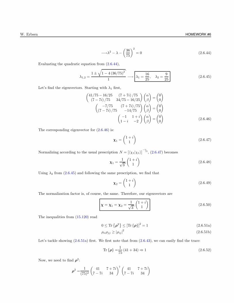
W. Erbsen HOMEWORK #6
−→λ2 − λ −(
36
75
)2
= 0 (2.6.44)
Evaluating the quadratic equation from (2.6.44),
λ1,2 =1 ±
√1 − 4 (36/75)
2
1−→ λ1 =
16
25, λ2 =
9
25(2.6.45)
Let’s find the eigenvectors. Starting with λ1 first,(
41/75− 16/25 (7 + 7i) /75(7 − 7i) /75 34/75− 16/25
)(αβ
)=
(00
)
(−7/75 (7 + 7i) /75
(7 − 7i) /75 −14/75
)(αβ
)=
(00
)
(−1 1 + i
1 − i −2
)(αβ
)=
(00
)(2.6.46)
The corresponding eigenvector for (2.6.46) is:
χ1 =
(1 + i
1
)(2.6.47)
Normalizing according to the usual prescription N = [〈χ1|χ1〉]−1/2 , (2.6.47) becomes
χ1 =1√3
(1 + i
1
)(2.6.48)
Using λ2 from (2.6.45) and following the same prescription, we find that
χ2 =
(1 + i
1
)(2.6.49)
The normalization factor is, of course, the same. Therefore, our eigenvectors are
χ = χ1 = χ2 =1√3
(1 + i
1
)(2.6.50)
The inequalities from (15.120) read
0 ≤ Trρ2≤ [Trρ]2 = 1 (2.6.51a)
ρiiρjj ≥ |ρij |2 (2.6.51b)
Let’s tackle showing (2.6.51a) first. We first note that from (2.6.43), we can easily find the trace:
Tr ρ =1
75(41 + 34) ⇒ 1 (2.6.52)
Now, we need to find ρ2:
ρ2 =1
(75)2
(41 7 + 7i
7 − 7i 34
)† (41 7 + 7i
7 − 7i 34
)
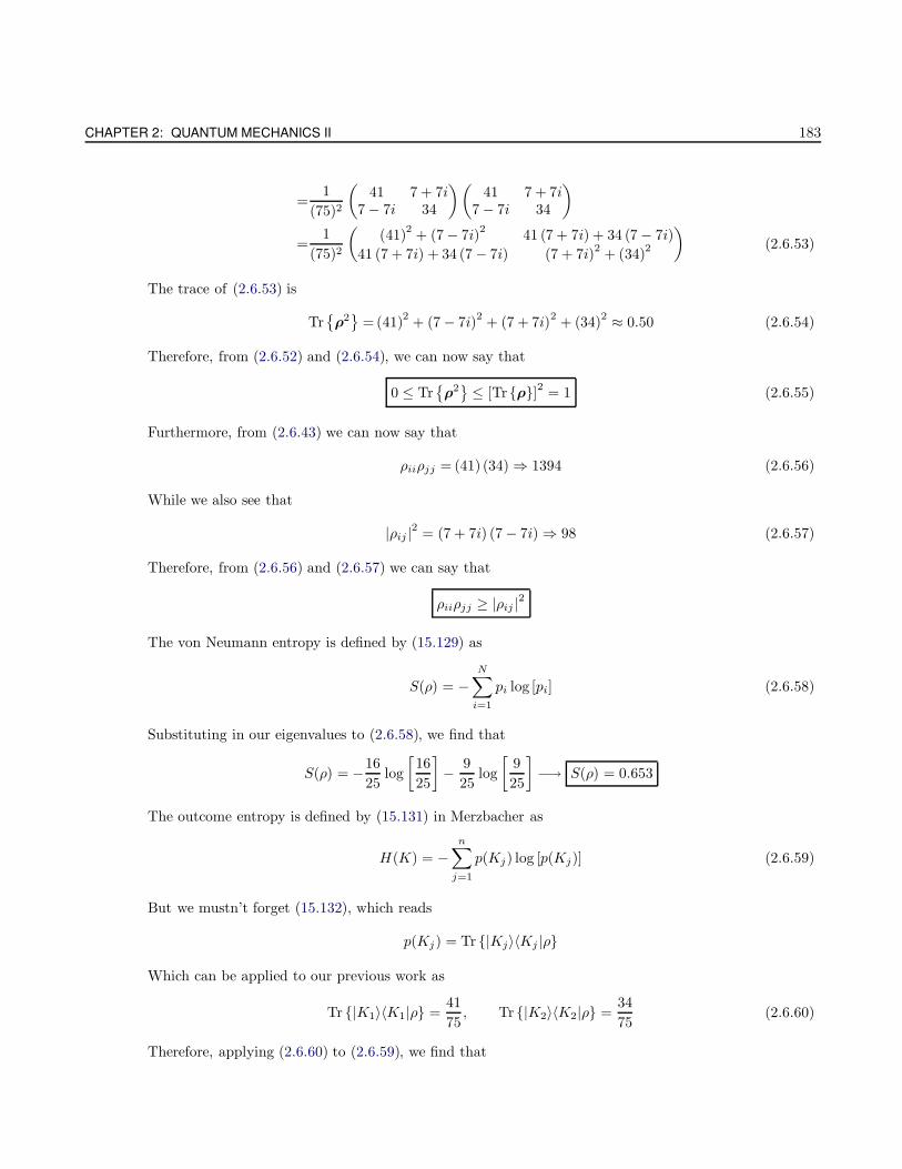
CHAPTER 2: QUANTUM MECHANICS II 183
=1
(75)2
(41 7 + 7i
7 − 7i 34
)(41 7 + 7i
7 − 7i 34
)
=1
(75)2
((41)
2+ (7 − 7i)
241 (7 + 7i) + 34 (7 − 7i)
41 (7 + 7i) + 34 (7 − 7i) (7 + 7i)2
+ (34)2
)(2.6.53)
The trace of (2.6.53) is
Trρ2
=(41)2
+ (7 − 7i)2
+ (7 + 7i)2
+ (34)2 ≈ 0.50 (2.6.54)
Therefore, from (2.6.52) and (2.6.54), we can now say that
0 ≤ Trρ2≤ [Trρ]2 = 1 (2.6.55)
Furthermore, from (2.6.43) we can now say that
ρiiρjj = (41) (34) ⇒ 1394 (2.6.56)
While we also see that
|ρij |2 = (7 + 7i) (7 − 7i) ⇒ 98 (2.6.57)
Therefore, from (2.6.56) and (2.6.57) we can say that
ρiiρjj ≥ |ρij |2
The von Neumann entropy is defined by (15.129) as
S(ρ) = −N∑
i=1
pi log [pi] (2.6.58)
Substituting in our eigenvalues to (2.6.58), we find that
S(ρ) = −16
25log
[16
25
]− 9
25log
[9
25
]−→ S(ρ) = 0.653
The outcome entropy is defined by (15.131) in Merzbacher as
H(K) = −n∑
j=1
p(Kj) log [p(Kj)] (2.6.59)
But we mustn’t forget (15.132), which reads
p(Kj) = Tr |Kj〉〈Kj |ρ
Which can be applied to our previous work as
Tr |K1〉〈K1|ρ =41
75, Tr |K2〉〈K2|ρ =
34
75(2.6.60)
Therefore, applying (2.6.60) to (2.6.59), we find that
W. Erbsen HOMEWORK #6
H(K) = −41
75log
[41
75
]− 34
75log
[34
75
]−→ H(K) = 0.688 (2.6.61)
To find the probability of measuring χ(z)+ , we first must evaluate
〈χ(z)+ |σz|χ(z)
+ 〉 =1
3
(1 − i 1
)(1 00 −1
)(1 + i
1
)
=1
3
(1 − i−1
)(1 + i
1
)
=1
3(1 − i) (1 + i) − 1
=1
3
We see here that the outcome entropy is larger than the result from a measurement of σz . Realizing
now that I may have misinterpreted this last part of the problem, we can also say that
H(K) > S(ρ)
Problem 16.1a
The spin-zero neutral kaon is a system with two basis states, the eigenstates of σz, representing a particle K0
and its antiparticle K0: The operator σx = CP represents the combined parity (P ) and charge conjugation (C),or particle-anti-particle, transformation and takes α = |K0〉 into β = |K0〉. The dynamics is governed by theHamiltonian matrix
H = M− iΓ
2(2.6.62)
Where M and Γ are Hermitian 2 × 2 matrices, representing the mass-energy and decay properties of the system,respectively. The matrix Γ is positive definite. A fundamental symmetry (under combined CP and time reversaltransformations) requires that σxM
∗ = Mσx and σxΓ∗ = Γσx.
Show that in the expansion of H in terms of the Pauli matrices, the matrix σz is absent. Derive the eigenvaluesand eigenstates of H in terms of the matrix elements of M and Γ. Are the eigenstates orthogonal?∗
Solution
Charge-parity reversal requires that σx|K0〉 = 1|K0〉. Furthermore, we recall that the four matrices 1,σx, σy and σz are linearally dependent, and any 2 × 2 matrix can be represented as
A = λ01 + λ1σx + λ2σy + λ3σz
Which is (16.57) from Merzbacher. Applying this principle to our matrix M,
∗What’s your favorite color?
CHAPTER 2: QUANTUM MECHANICS II 185
M =a11+ b1σx + c1σy + d1σz
=a1
(1 00 1
)+ b1
(0 11 0
)+ c1
(0 −ii 0
)+ d1
(1 00 −1
)
=
(a1 + d1 b1 − ic1b1 + ic1 a1 − d1
)(2.6.63)
We recall from the prompt that σxM∗ = Mσx, which is a requirement. Applying the LHS of this
statement to our matrix M from (2.6.63),
σxM∗ =
(0 11 0
)(a1 + d1 b1 − ic1b1 + ic1 a1 − d1
)∗⇒(
0 11 0
)(a1 + d1 b1 + ic1b1 − ic1 a1 − d1
)(2.6.64)
We now compute the RHS of our statement:
Mσx =
(a1 + d1 b1 − ic1b1 + ic1 a1 − d1
)(0 11 0
)⇒(b1 − ic1 a1 + d1
a1 − d1 b1 + ic1
)(2.6.65)
So, equating (2.6.64) and (2.6.65),
σxM∗ = Mσx −→
(b1 − ic1 a1 − d1
a1 + d1 b1 + ic1
)=
(b1 − ic1 a1 + d1
a1 − d1 b1 + ic1
)(2.6.66)
This yields two equations,
b1 − ic1 + a1 − d1 = b1 − ic1 + a1 + d1 −→ −d1 = d1 (2.6.67a)
a1 + d1 + b1 + ic1 = a1 − d1 + b1 + ic1 −→ d1 = −d1 (2.6.67b)
We see that in order for M to meet the requirement that σxM∗ = Mσx, we must have d1 = 0. We can
rewrite M from (2.6.63) with this change,
M =
(a1 b1 − ic1
b1 + ic1 a1
)(2.6.68)
We can equally well apply this principle to the matrix Γ:
Γ =
(a2 + d2 b2 − ic2b2 + ic2 a2 − d2
)(2.6.69)
Following the logic which led us to (2.6.68), we may use (2.6.69) to deduce that d2 = 0 according to therequirement that σxΓ
∗ = Γσx, and we can now write
Γ =
(a2 b2 − ic2
b2 + ic2 a2
)(2.6.70)
We now substitute (2.6.68) and (2.6.70) into (2.6.62),
H =
(a1 b1 − ic1
b1 + ic1 a1
)− i
2
(a2 b2 − ic2
b2 + ic2 a2
)
=
(a1 b1 − ic1
b1 + ic1 a1
)−(
i/2 · a2i/2 (b2 − ic2)
i/2 (b2 + ic2)i/2 · a2
)
W. Erbsen HOMEWORK #6
=
(a1 b1 − ic1
b1 + ic1 a1
)−(
ia2/2 (ib2 + c2) /2(ib2 − c2) /2 ia2/2
)
=
(a1 − ia2/2 b1 − ic1 − (ib2 + c2) /2
b1 + ic1 − (ib2 − c2) /2 a1 − ia2/2
)(2.6.71)
We must now find the eigenvalues of H, in the usual way∣∣∣∣
a1 − ia2/2 − λ b1 − ic1 − (ib2 + c2) /2b1 + ic1 − (ib2 − c2) /2 a1 − ia2/2 − λ
∣∣∣∣ =0
(a1 − i/2a2 − λ
)2 −(b1 − ic1 − 1/2 (ib2 + c2)
) (b1 + ic1 − 1/2 (ib2 − c2)
)=0 (2.6.72)
We can just go ahead and solve for λ,
λ = a1 − i/2a2 ±√
(b1 − ic1 − 1/2 (ib2 + c2)) (b1 + ic1 − 1/2 (ib2 − c2)) (2.6.73)
We can simplify (2.6.73) ever so slightly, giving eigenvalues
λ1,2 = a1 − i/2a2 −√
(2b1 − ib2)2
+ (2c1 − ic2)2
(2.6.74)
To find the eigenvectors, we substitute λ1 and λ2 from (2.6.74) into our Hamiltonian from (2.6.72) as(
a1 − ia2/2 − λ1,2 b1 − ic1 − (ib2 + c2) /2b1 + ic1 − (ib2 − c2) /2 a1 − ia2/2 − λ1,2
)(c1c2
)=
(00
)(2.6.75)
The eigenvectors were found using Mathematica. The result is
χ1,2 = N
(±√
(2b1−ib2)2+(2c1−ic2)
2
2b1−ib2+2ic1+c2
1
)(2.6.76)
The normalization in (2.6.76) is obtained as we usually do:
〈χ1|χ1〉 = 1 −→ N2χ†1 · χ1 = 1 −→ N2
(c1 c2
)∗(c1c2
)= 1 −→ N =
1√c∗1c1 + c∗2c2
(2.6.77)
This normalization constant was determined from (2.6.77) using Mathematica, the result is
N =
√(2b1 + ib2)
2 + (2c1 + ic2)2
2b1 + ib2 − 2ic1 + c2+
√(2b1 − ib2)
2 + (2c1 − ic2)2
2b1 − ib2 + 2ic1 + c2
−1/2
(2.6.78)
Combining (2.6.76) and (2.6.78), the normalized eigenvectors are
χ1,2 =
√(2b1 + ib2)
2+ (2c1 + ic2)
2
2b1 + ib2 − 2ic1 + c2+
√(2b1 − ib2)
2+ (2c1 − ic2)
2
2b1 − ib2 + 2ic1 + c2
−1/2 (±√
(2b1−ib2)2+(2c1−ic2)
2
2b1−ib2+2ic1+c2
1
)
(2.6.79)
To see if the eigenstates from (2.6.79) are orthogonal, we apply the following test:
CHAPTER 2: QUANTUM MECHANICS II 187
〈χ1|χ2〉 = 0 (if orthogonal) (2.6.80)
Using Mathematica, it is easy to show that (2.6.80) is not satisfied, and therefore χ1 and χ2 are not orthogonal .
2.7 Homework #7
Exercise 17.12
Derive the recursion relation (17.54), as indicated.
Solution
We first recall three three relations defining various quantities specifying the behavior of the total angularmomentum:
J =J1 + J2
Jz =Jz1 + Jz2
J+ =J1+ + J2+ (2.7.1a)
We now recall the three equations from (17.27) of Merzbacher:
Jz|j m〉 =m~|j m〉 (2.7.2a)
J+|j m〉 =√
(j −m)(j +m+ 1) ~ |j1 j2 j m+ 1〉 (2.7.2b)
J−|j m〉 =√
(j +m)(j −m+ 1) ~ |j1 j2 j m− 1〉 (2.7.2c)
We also recall (17.52), which reads
|j1 j2 j m〉 =∑
m1,m2
|j1 j2 m1 m2〉〈j1 j2 m1 m2|j1 j2 j m〉 (2.7.3)
Which is the link between the direct product basis and the total angular momentum basis. Accordingto Merzbacher, in order to obtain the recursion relations from (17.54), all we have to do is apply J+
and J− to (2.7.3). The behavior of J+ and J− is defined by (2.7.2b) and (2.7.2c), which may be morecompactly redefined as
J±|j m〉 =√
(j ∓m)(j ±m+ 1) ~ |j1 j2 j m± 1〉 (2.7.4)
Similarly, we may generalize (2.7.1a) as
J± = J1± + J2± (2.7.5)
We can apply (2.7.5) to (2.7.3), which yields
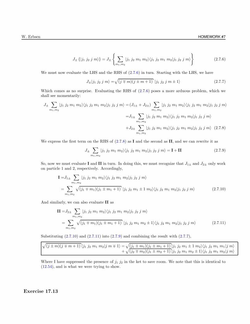
W. Erbsen HOMEWORK #7
J± |j1 j2 j m〉 = J±
∑
m1,m2
|j1 j2 m1 m2〉〈j1 j2 m1 m2|j1 j2 j m〉
(2.7.6)
We must now evaluate the LHS and the RHS of (2.7.6) in turn. Starting with the LHS, we have
J±|j1 j2 j m〉 =√
(j ∓m)(j ±m+ 1) |j1 j2 j m± 1〉 (2.7.7)
Which comes as no surprise. Evaluating the RHS of (2.7.6) poses a more arduous problem, which weshall see momentarily:
J±∑
m1,m2
|j1 j2 m1 m2〉〈j1 j2 m1 m2|j1 j2 j m〉 =(J1± + J2±)∑
m1,m2
|j1 j2 m1 m2〉〈j1 j2 m1 m2|j1 j2 j m〉
=J1±∑
m1,m2
|j1 j2 m1 m2〉〈j1 j2 m1 m2|j1 j2 j m〉
+J2±∑
m1,m2
|j1 j2 m1 m2〉〈j1 j2 m1 m2|j1 j2 j m〉 (2.7.8)
We express the first term on the RHS of (2.7.8) as I and the second as II, and we can rewrite it as
J±∑
m1,m2
|j1 j2 m1 m2〉〈j1 j2 m1 m2 |j1 j2 j m〉 = I + II (2.7.9)
So, now we must evaluate I and II in turn. In doing this, we must recognize that J1± and J2± only workon particle 1 and 2, respectively. Accordingly,
I =J1±∑
m1,m2
|j1 j2 m1 m2〉〈j1 j2 m1 m2|j1 j2 j m〉
=∑
m1,m2
√(j1 ∓m1)(j1 ±m1 + 1) |j1 j2 m1 ± 1 m2〉〈j1 j2 m1 m2|j1 j2 j m〉 (2.7.10)
And similarly, we can also evaluate II as
II =J2±∑
m1,m2
|j1 j2 m1 m2〉〈j1 j2 m1 m2|j1 j2 j m〉
=∑
m1,m2
√(j1 ∓m1)(j1 ±m1 + 1) |j1 j2 m1 m2 ± 1〉〈j1 j2 m1 m2|j1 j2 j m〉 (2.7.11)
Substituting (2.7.10) and (2.7.11) into (2.7.9) and combining the result with (2.7.7),
√(j ±m)(j ∓m+ 1) 〈j1 j2 m1 m2|j m∓ 1〉 =
√(j1 ±m1)(j1 ±m1 + 1) |j1 j2 m1 ± 1 m2〉〈j1 j2 m1 m1 |j m〉
+√
(j2 ∓m2)(j1 ±m2 + 1) |j1 j2 m1 m2 ± 1〉〈j1 j2 m1 m2 |j m〉
Where I have suppressed the presence of j1 j2 in the ket to save room. We note that this is identical to(12.54), and is what we were trying to show.
Exercise 17.13
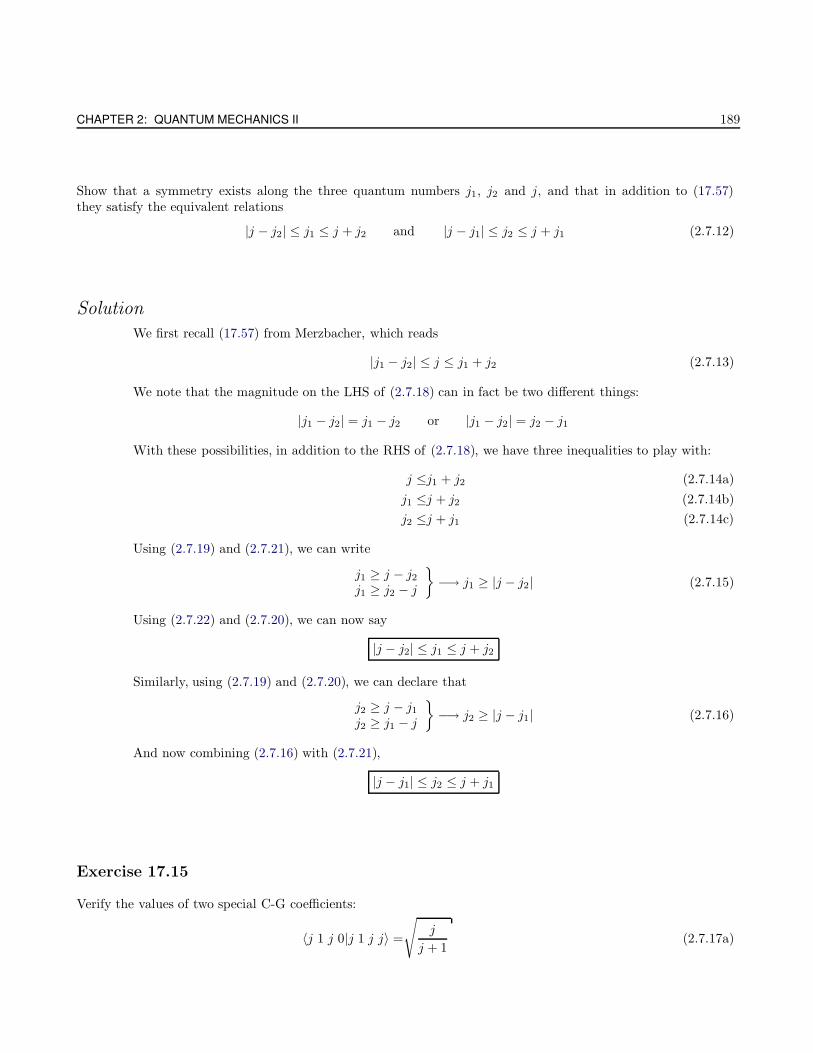
CHAPTER 2: QUANTUM MECHANICS II 189
Show that a symmetry exists along the three quantum numbers j1, j2 and j, and that in addition to (17.57)they satisfy the equivalent relations
|j − j2| ≤ j1 ≤ j + j2 and |j − j1| ≤ j2 ≤ j + j1 (2.7.12)
Solution
We first recall (17.57) from Merzbacher, which reads
|j1 − j2| ≤ j ≤ j1 + j2 (2.7.13)
We note that the magnitude on the LHS of (2.7.18) can in fact be two different things:
|j1 − j2| = j1 − j2 or |j1 − j2| = j2 − j1
With these possibilities, in addition to the RHS of (2.7.18), we have three inequalities to play with:
j ≤j1 + j2 (2.7.14a)
j1 ≤j + j2 (2.7.14b)
j2 ≤j + j1 (2.7.14c)
Using (2.7.19) and (2.7.21), we can write
j1 ≥ j − j2j1 ≥ j2 − j
−→ j1 ≥ |j − j2| (2.7.15)
Using (2.7.22) and (2.7.20), we can now say
|j − j2| ≤ j1 ≤ j + j2
Similarly, using (2.7.19) and (2.7.20), we can declare that
j2 ≥ j − j1j2 ≥ j1 − j
−→ j2 ≥ |j − j1| (2.7.16)
And now combining (2.7.16) with (2.7.21),
|j − j1| ≤ j2 ≤ j + j1
Exercise 17.15
Verify the values of two special C-G coefficients:
〈j 1 j 0|j 1 j j〉 =
√j
j + 1(2.7.17a)
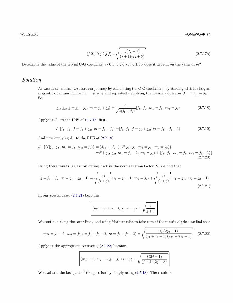
W. Erbsen HOMEWORK #7
〈j 2 j 0|j 2 j j〉 =
√j(2j − 1)
(j + 1)(2j + 3)(2.7.17b)
Determine the value of the trivial C-G coefficient 〈j 0 m 0|j 0 j m〉. How does it depend on the value of m?
Solution
As was done in class, we start our journey by calculating the C-G coefficients by starting with the largestmagnetic quantum number m = j1 + j2 and repeatedly applying the lowering operator J− = J1+ + J2−.So,
|j1, j2, j = j1 + j2, m = j1 + j2〉 =~√
2(j1 + j2)|j1, j2, m1 = j1, m2 = j2〉 (2.7.18)
Applying J− to the LHS of (2.7.18) first,
J−|j1, j2, j = j1 + j2, m = j1 + j2〉 =|j1, j2, j = j1 + j2, m = j1 + j2 − 1〉 (2.7.19)
And now applying J− to the RHS of (2.7.18),
J− N |j1, j2, m1 = j1, m2 = j2〉 = (J1+ + J2−) N |j1, j2, m1 = j1, m2 = j2〉=N |j1, j2, m1 = j1 − 1, m2 = j2〉 + |j1, j2, m1 = j1, m2 = j2 − 1〉
(2.7.20)
Using these results, and substituting back in the normalization factor N , we find that
|j = j1 + j2, m = j1 + j2 − 1〉 =
√j1
j1 + j2|m1 = j1 − 1, m2 = j2〉 +
√j2
j1 + j2|m1 = j1, m2 = j2 − 1〉
(2.7.21)
In our special case, (2.7.21) becomes
〈m1 = j, m2 = 0|j, m = j〉 =
√j
j + 1
We continue along the same lines, and using Mathematica to take care of the matrix algebra we find that
〈m1 = j1 − 2, m2 = j2|j = j1 + j2 − 2, m = j1 + j2 − 2〉 =
√j2 (2j2 − 1)
(j1 + j2 − 1) (2j1 + 2j2 − 1)(2.7.22)
Applying the appropriate constants, (2.7.22) becomes
〈m1 = j, m2 = 2|j = j, m = j〉 =
√j (2j − 1)
(j + 1) (2j + 3)
We evaluate the last part of the question by simply using (2.7.18). The result is
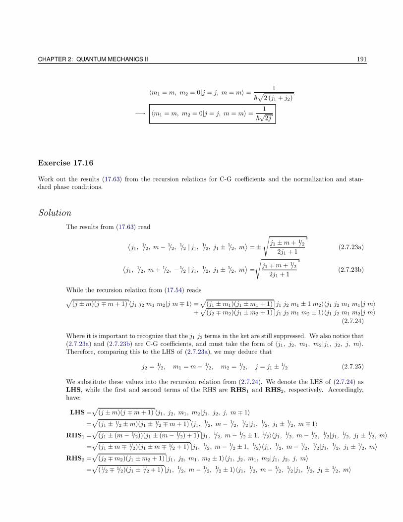
CHAPTER 2: QUANTUM MECHANICS II 191
〈m1 = m, m2 = 0|j = j, m = m〉 =1
~√
2 (j1 + j2)
−→ 〈m1 = m, m2 = 0|j = j, m = m〉 =1
~√
2j
Exercise 17.16
Work out the results (17.63) from the recursion relations for C-G coefficients and the normalization and stan-dard phase conditions.
Solution
The results from (17.63) read
⟨j1,
1/2, m− 1/2,1/2 | j1, 1/2, j1 ± 1/2, m
⟩= ±
√j1 ±m+ 1/2
2j1 + 1(2.7.23a)
⟨j1,
1/2, m+ 1/2, −1/2 | j1, 1/2, j1 ± 1/2, m⟩
=
√j1 ∓m+ 1/2
2j1 + 1(2.7.23b)
While the recursion relation from (17.54) reads
√(j ±m)(j ∓m+ 1) 〈j1 j2 m1 m2|j m∓ 1〉 =
√(j1 ±m1)(j1 ±m1 + 1) |j1 j2 m1 ± 1 m2〉〈j1 j2 m1 m1|j m〉
+√
(j2 ∓m2)(j1 ±m2 + 1) |j1 j2 m1 m2 ± 1〉〈j1 j2 m1 m2|j m〉(2.7.24)
Where it is important to recognize that the j1 j2 terms in the ket are still suppressed. We also notice that(2.7.23a) and (2.7.23b) are C-G coefficients, and must take the form of 〈j1, j2, m1, m2|j1, j2, j, m〉.Therefore, comparing this to the LHS of (2.7.23a), we may deduce that
j2 = 1/2, m1 = m− 1/2, m2 = 1/2, j = j1 ± 1/2 (2.7.25)
We substitute these values into the recursion relation from (2.7.24). We denote the LHS of (2.7.24) asLHS, while the first and second terms of the RHS are RHS1 and RHS2, respectively. Accordingly,have:
LHS =√
(j ±m)(j ∓m+ 1) 〈j1, j2, m1, m2|j1, j2, j, m∓ 1〉=√
(j1 ± 1/2 ±m)(j1 ± 1/2 ∓m+ 1) 〈j1, 1/2, m− 1/2,1/2|j1, 1/2, j1 ± 1/2, m∓ 1〉
RHS1 =√
(j1 ± (m− 1/2))(j1 ± (m− 1/2) + 1) |j1, 1/2, m− 1/2 ± 1, 1/2〉〈j1, 1/2, m− 1/2,1/2|j1, 1/2, j1 ± 1/2, m〉
=√
(j1 ±m∓ 1/2)(j1 ±m∓ 1/2 + 1) |j1, 1/2, m− 1/2 ± 1, 1/2〉〈j1, 1/2, m− 1/2,1/2|j1, 1/2, j1 ± 1/2, m〉
RHS2 =√
(j2 ∓m2)(j1 ±m2 + 1) |j1, j2, m1, m2 ± 1〉〈j1, j2, m1, m2|j1, j2, j, m〉=√
(1/2 ∓ 1/2)(j1 ± 1/2 + 1) |j1, 1/2, m− 1/2,1/2 ± 1〉〈j1, 1/2, m− 1/2,
1/2|j1, 1/2, j1 ± 1/2, m〉
W. Erbsen HOMEWORK #7
Seemingly arbitrarily, we choose the top sign in the above equations:
LHS =√
(j1 +m+ 1/2) (j1 −m+ 3/2) 〈j1, 1/2, m− 1/2,1/2|j1 + 1/2, m1〉
RHS1 =√
(j1 +m− 1/2) (j1 +m+ 1/2) |j1, 1/2, m+ 1/2,1/2〉〈j1, 1/2, m− 1/2,
1/2|j1 + 1/2, m〉RHS2 =0
Combining these equations and rearranging,
〈m− 1/2,1/2|j1 + 1/2, m〉 =
√j1 +m+ 1/2j1 +m+ 3/2
〈m+ 1/2,1/2|j1 + 1/2, m+ 1〉 (2.7.26)
Shifting the index according to m→ m+ 1, we now have
〈m+ 1/2,1/2|j1 + 1/2, m+ 1〉 =
√j1 +m+ 3/2j1 +m+ 5/2
〈m+ 3/2,1/2|j1 + 1/2, m+ 2〉 (2.7.27)
Going back to (2.7.23a) and applying m = j1 + 1/2 to (2.7.26) and (2.7.27), we find that
〈j1, 1/2, m− 1/2,1/2|j1, 1/2, j1 − 1/2, m〉 = ±
√j1 +m+ 1/2
2j1 + 1(2.7.28)
Substituting back in the appropriate ± signs into (2.7.28),
⟨j1,
1/2, m− 1/2,1/2 | j1, 1/2, j1 ± 1/2, m
⟩= ±
√j1 ±m+ 1/2
2j1 + 1(2.7.29)
Which we note is identical to (2.7.23a). To derive (2.7.23b), we repeat the same process. Evaluating theLHS and RHS of our recursion relation yields
LHS =√
(j1 ± 1/2 ±m)(j1 ± 1/2 ∓m+ 1) 〈j1, 1/2, m+ 1/2, −1/2|j1 ± 1/2, m∓ 1〉RHS1 =
√(j1 ± (m+ 1/2))(j1 ± (m+ 1/2) + 1) |j1, 1/2, m+ 1/2 ± 1, −1/2〉〈j1, 1/2, m+ 1/2, −1/2|j1 ± 1/2, m〉
RHS2 =√
(1/2 ∓ (−1/2))(j1 ± (−1/2) + 1) |j1, 1/2, m+ 1/2, −1/2 ± 1〉〈j1, 1/2, m+ 1/2, −1/2|j1 ± 1/2, m〉
The steps taken to arrive at (2.7.23b) are from henceforth identical to that which was done to derive(2.7.23a), and accordingly they will not be shown. From the above equations, we choose an arbitrarysign (which will be stuck back in at the end) in order to simplify the equation. We then shift the indexof m, finagle the equations and evaluating the coefficient in terms of j1 and m, we get
⟨j1,
1/2, m+ 1/2, −1/2 | j1, 1/2, j1 ± 1/2, m⟩
=
√j1 ∓m+ 1/2
2j1 + 1
Which is of course (2.7.23b).
Exercise 17.18
CHAPTER 2: QUANTUM MECHANICS II 193
Starting with the uncoupled basis (17.67), work out the 4 × 4 matrices Sz and S2, and show by explicit diag-onalzation that the singlet and triplet states are the eigenvectors with the appropriate eigenvalues.
Solution
We recall that (17.67) from Merzbacher reads
α1 ⊗ α2 = α1α2, α1 ⊗ β2 = α1β2, β1 ⊗ α2 = β1α2, β1 ⊗ β2 = β1β2 (2.7.30)
We introduce the following shorthand notation, as indicated in lecture, which constitutes the productbasis:
|++〉, |+−〉, |−+〉, |−−〉
Where the first term in each ket acts on particle 1, while the second acts on particle 2. We also recallthat we can write the total spin operator S in terms of the single particle spin operators S1 and S2 as
S = S1 ⊗ 1(2) + 1
(1) ⊗ S2 (2.7.31)
We also note that when referring to the individual components of the spin operators, it will be mostconvenient to work in terms of the raising and lowering spin operators (S+ and S−, respectively). Theraising and lowering operators are described in terms of the cartesian components by
S± = Sz ± iSy
So that S (Sx, Sy, Sz) → S (S±, Sz). We now recognize that the S acts on the individual spin ketsaccording to
Sz|+〉 = ~/2|+〉, Sz |−〉 = −~/2|−〉S+|+〉 = 0, S+|−〉 = ~|+〉S−|+〉 = ~|−〉, S−|−〉 = 0
We also musn’t forget how the total components act on each particle, following the convention of (2.7.31),
Sz =S1z ⊗ 1(2) + 1
(1) ⊗ S2z
S+ =S1+ ⊗ 1(2) + 1
(1) ⊗ S2+
S− =S1− ⊗ 1(2) + 1
(1) ⊗ S2−
Accordingly, we can now write
Sz |++〉 =~/2|++〉 + ~/2|++〉 ⇒ ~|++〉 (2.7.32a)
Sz |+−〉 =0 (2.7.32b)
Sz |−+〉 =0 (2.7.32c)
Sz |−−〉 = − ~/2|−−〉 − ~/2|−−〉 ⇒ −~|−−〉 (2.7.32d)
We can express (2.7.32a)-(2.7.32d) in matrix form as
W. Erbsen HOMEWORK #7
(Sz)m1,m2=
~ 0 0 00 0 0 00 0 0 00 0 0 −~
(2.7.33)
The value of the eigenvalues from (2.7.34) are transparent,
λ1 = ~, λ2 = −~
We now wish to find S2, first representing it in the product basis:
S2 =S21 + S2
2 + 2S1zS2z + S1+S2− + S1−S2+ (2.7.34)
In order to evaluate all the matrix elements for S2, let’s make a table:
S21 S2
2 S1z S2z S1+ S2− S1− S2+
|++〉 3/4~2|++〉 3/4~
2|++〉 1/2~|++〉 1/2~|++〉 0 ~|+〉 ~|+〉 0|+−〉 3/4~
2|+−〉 3/4~2|+−〉 1/2~|+−〉 −1/2~|+−〉 0 0 ~|−〉 ~|+〉
|−+〉 3/4~2|−+〉 3/4~
2|−+〉 −1/2~|−+〉 1/2~|−+〉 ~|+〉 ~|−〉 0 0|−−〉 3/4~
2|−−〉 3/4~2|−−〉 −1/2~|−−〉 −1/2~|−−〉 ~|+〉 0 0 ~|−〉
Substituting the values of the tabulated matrix elements into (2.7.34), we find that:
S2|++〉 =3/4~2|++〉 + 3/4~
2|++〉 + 2(
1/2~|++〉) (
1/2~|++〉)⇒ 2~2|++〉 (2.7.35a)
S2|+−〉 =3/4~2|+−〉 + 3/4~
2|+−〉 + 2(
1/2~|+−〉) (
−1/2~|+−〉)
+ ~2|−+〉 ⇒ ~2 (|+−〉 + |−+) (2.7.35b)
S2|−+〉 =3/4~2|−+〉 + 3/4~
2|−+〉 + 2(−1/2~|−+〉
) (1/2~|−+〉
)+ ~2|+−〉 ⇒ ~2 (|−+〉 + |+−〉) (2.7.35c)
S2|−−〉 =3/4~2|−−〉 + 3/4~
2|−−〉 + 2(−1/2~|−−〉
) (−1/2~|−−〉
)⇒ 2~2|−−〉 (2.7.35d)
We can find the expectation values of S2 (i.e. the matrix elements) easily, and the non-zero elements are
〈+ + |S2|++〉 =2~2
〈+ − |S2|+−〉 =~2
〈+ − |S2|−+〉 =~2
〈− + |S2|+−〉 =~2
〈− + |S2|−+〉 =~2
〈+ + |S2|++〉 =2~2
While all the other elements are of course zero. We are now in a place to write down the matrix S2:
(S2)m1,m2
= ~2
2 0 0 00 1 1 00 1 1 00 0 0 2
(2.7.36)
Which is not diagonal. We can remedy this by diagonalizing the central matrix, allowing us to find theeigenvalues and eigenvectors of S2.
CHAPTER 2: QUANTUM MECHANICS II 195
(S′)2
=
(~2 ~2
~2 ~2
)
Finding the eigenvalues,∣∣∣∣~2 − λ ~2
~2 ~2 − λ
∣∣∣∣ = 0 −→(~2 − λ
) (~2 − λ
)− ~4 = 0
−→λ(λ− 2~2
)= 0
−→ λ1 = 0, λ2 = 2~2
Whose corresponding eigenvectors are
V1 =1√2
(|+−〉 − |−+〉) , V2 =1√2
(|+−〉 + |−+〉)
The eigenvectors which we did not include here are found from the first and fourth column of the matrixS2. Combining the results, we arrive at a series of states whose total angular momentum is either 0 or1, i.e. either singlet or triplet. The states are
|0 0〉 =1√2
(|+−〉 − |−+〉)
|1 m〉 = |++〉
|1 m〉 =1√2
(|+−〉 + |−+〉)
|1 m〉 = |−−〉
Problem 17.1
In the notation of (17.64) the state of a spin one-half particle with sharp total angular momentum j, m is
aY jmj−1/2
+ bY jmj+1/2
(2.7.37)
Assume this state to be an eigenstate of the Hamiltonian with no degeneracy other than that demanded byrotational invariance.
a) If H conserves parity, how are the coefficients a and b restricted?
b) If H is invariant under time reversal, show that a/b must be imaginary.
c) Verify explicitly that the expectation value of the electric dipole moment −e r vanishes if either parity isconserved or time reversal invariance holds (or both).
Solution
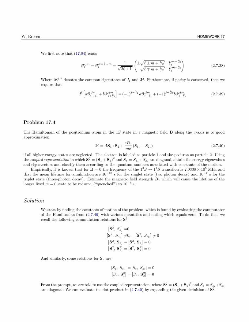
W. Erbsen HOMEWORK #7
We first note that (17.64) reads
Yjm
` = Y`±1/2, m
` =1√
2`+ 1
(±√` ±m+ 1/2 Y
m−1/2`√
` ∓m+ 1/2 Ym+1/2
`
)(2.7.38)
Where Yjm
` denotes the common eigenstates of Jz and J2. Furthermore, if parity is conserved, then werequire that
P[aY jm
j−1/2+ bY jm
1+1/2
]=(−1)
j−1/2 aY jmj−1/2
+ (−1)j+1/2 bY jm
j+1/2(2.7.39)
Problem 17.4
The Hamiltonain of the positronium atom in the 1S state in a magnetic field B along the z-axis is to goodapproximation
H = AS1 · S2 +eB0
mc(S1z − S2z) (2.7.40)
if all higher energy states are neglected. The electron is labeled as particle 1 and the positron as particle 2. Usingthe coupled representation in which S2 = (S1 + S2)
2and Sz = S1z +S2z are diagonal, obtain the energy eigenvalues
and eigenvectors and classify them according to the quantum numbers associated with constants of the motion.Empirically, it is known that for B = 0 the frequency of the 13S → 11S transition is 2.0338× 10⁵ MHz and
that the mean lifetime for annihilation are 10−10 s for the singlet state (two photon decay) and 10−7 s for thetriplet state (three-photon decay). Estimate the magnetic field strength B0 which will cause the lifetime of thelonger lived m = 0 state to be reduced (“quenched”) to 10−8 s.
Solution
We start by finding the constants of motion of the problem, which is found by evaluating the commutatorof the Hamiltonian from (2.7.40) with various quantities and noting which equals zero. To do this, werecall the following commutation relations for S2:
[S2, Sz
]=0
[S2, Sz1
]6=0,
[S2, Sz2
]6= 0
[S2, S1
]=[S2, S2
]= 0
[S2, S2
1
]=[S2, S2
2
]= 0
And similarly, some relations for Sz are
[Sz , Sz1 ] = [Sz , Sz2 ] = 0[Sz , S2
1
]=[Sz , S2
2
]= 0
From the prompt, we are told to use the coupled representation, where S2 = (S1 + S2)2 and Sz = Sz1+Sz2
are diagonal. We can evaluate the dot product in (2.7.40) by expanding the given definition of S2:

CHAPTER 2: QUANTUM MECHANICS II 197
S2 = (S1 + S2)2 ⇒ S2
1 + S22 + 2S1 · S2 −→ S1 · S2 = 1/2
(S2 − S2
1 − S22
)(2.7.41)
Substituting (2.7.41) into (2.7.40), the Hamiltonian becomes
H = 1/2A(S2 − S2
1 − S22
)+eB0
mc(S1z − S2z) (2.7.42)
Let’s not evaluate some commutators to find the constants of motion:
[H,S2
]=[
1/2A(S2 − S2
1 − S22
)+ ω (Sz1 − Sz2 )
, S2
]
=1/2A [
S2, S2]
︸ ︷︷ ︸=0
−[S2
1, S2]
︸ ︷︷ ︸=0
−[S2
2, S2]
︸ ︷︷ ︸=0
+ ω
[Sz1 , S2
]︸ ︷︷ ︸
6=0
−[Sz2 , S2
]︸ ︷︷ ︸
6=0
6= 0 (2.7.43)
[H, Sz] =[
1/2A(S2 − S2
1 − S22
)+ ω (Sz1 − Sz2 )
, Sz
]
=1/2A [
S2, Sz
]︸ ︷︷ ︸
=0
−[S2
1, Sz
]︸ ︷︷ ︸
=0
−[S2
2, Sz
]︸ ︷︷ ︸
=0
+ ω
[Sz1 , Sz ]︸ ︷︷ ︸
=0
− [Sz2 , Sz ]︸ ︷︷ ︸=0
= 0 (2.7.44)
[H,S1] =[
1/2A(S2 − S2
1 − S22
)+ ω (Sz1 − Sz2 )
, S1
]
=1/2A [
S2, S1
]︸ ︷︷ ︸
=0
−[S2
1, S1
]︸ ︷︷ ︸
=0
−[S2
2, S1
]︸ ︷︷ ︸
=0
+ ω
[Sz1 , S1]︸ ︷︷ ︸
=0
− [Sz2 , S1]︸ ︷︷ ︸=0
= 0 (2.7.45)
[H,S2] =[
1/2A(S2 − S2
1 − S22
)+ ω (Sz1 − Sz2 )
, S2
]
=1/2A [
S2, S2
]︸ ︷︷ ︸
=0
−[S2
1, S2
]︸ ︷︷ ︸
=0
−[S2
2, S2
]︸ ︷︷ ︸
=0
+ ω
[Sz1 , S2]︸ ︷︷ ︸
=0
− [Sz2 , S2]︸ ︷︷ ︸=0
= 0 (2.7.46)
So, S2 is not a constant of motion according to (2.7.43), while Sz , S1, and S2 are constants of motionfrom (2.7.44)-(2.7.46). We now wish to switch to the following basis notation,
|++〉, |+−〉, |−+〉, |−−〉
We now wish to evaluate the diagonal matrix elements for H, first recalling that
H = 1/2A(S2 − S2
1 − S22
)+ ω (S1z − S2z)
S2 S21 S2
1 S1z S2z
|++〉 2~2|++〉 3/4~2|++〉 3/4~
2|++〉 1/2~|++〉 1/2~|++〉|+−〉 0 3/4~
2|+−〉 3/4~2|+−〉 1/2~|+−〉 −1/2~|+−〉
|−+〉 0 3/4~2|−+〉 3/4~
2|−+〉 −1/2~|−+〉 1/2~|−+〉|−−〉 2~2|−−〉 3/4~
2|−−〉 3/4~2|−−〉 −1/2~|−−〉 −1/2~|−−〉
Substituting the tabulated elements into our Hamiltonian,
H|++〉 =1/2A(2~2 − 3/4~2 − 3/4~
2)|++〉 ⇒ 1/4A~2 |++〉
H|+−〉 =1/2A(−3/4~
2 − 3/4~2)|+−〉 + ω
(1/2~ + 1/2~
)|+−〉 ⇒
(−3/4A~2 + ω~
)|+−〉
H|−+〉 =1/2A(−3/4~
2 − 3/4~2)|−+〉 + ω
(−1/2~ − 1/2~
)|−+〉 ⇒
(−3/4A~2 − ω~
)|−+〉
H|−−〉 =1/2A(2~2 − 3/4~2 − 3/4~
2)|−−〉 ⇒ 1/4A~2 |−−〉
These calculations were clearly done in the direct product basis, whereas it could just as easily be donein the total angular momentum basis.
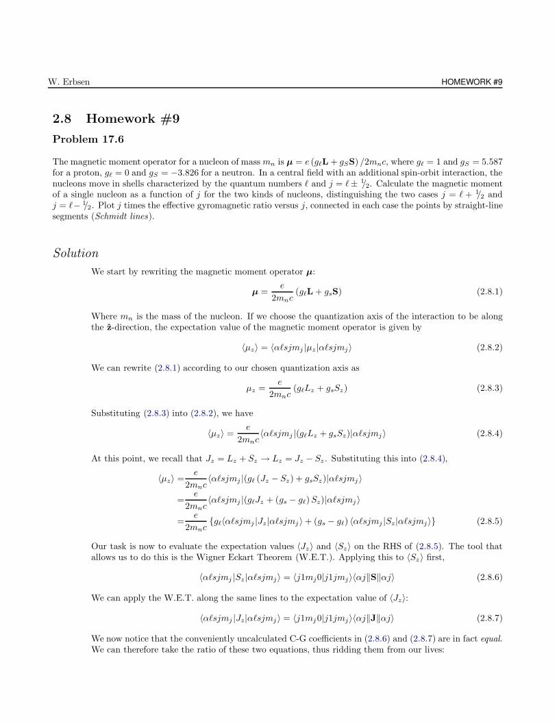
W. Erbsen HOMEWORK #9
2.8 Homework #9
Problem 17.6
The magnetic moment operator for a nucleon of mass mn is µ = e (g`L + gSS) /2mnc, where g` = 1 and gS = 5.587for a proton, g` = 0 and gS = −3.826 for a neutron. In a central field with an additional spin-orbit interaction, thenucleons move in shells characterized by the quantum numbers ` and j = `± 1/2. Calculate the magnetic momentof a single nucleon as a function of j for the two kinds of nucleons, distinguishing the two cases j = ` + 1/2 andj = `− 1/2. Plot j times the effective gyromagnetic ratio versus j, connected in each case the points by straight-linesegments (Schmidt lines).
Solution
We start by rewriting the magnetic moment operator µ:
µ =e
2mnc(g`L + gsS) (2.8.1)
Where mn is the mass of the nucleon. If we choose the quantization axis of the interaction to be alongthe z-direction, the expectation value of the magnetic moment operator is given by
〈µz〉 = 〈α`sjmj |µz|α`sjmj〉 (2.8.2)
We can rewrite (2.8.1) according to our chosen quantization axis as
µz =e
2mnc(g`Lz + gsSz) (2.8.3)
Substituting (2.8.3) into (2.8.2), we have
〈µz〉 =e
2mnc〈α`sjmj |(g`Lz + gsSz)|α`sjmj 〉 (2.8.4)
At this point, we recall that Jz = Lz + Sz → Lz = Jz − Sz . Substituting this into (2.8.4),
〈µz〉 =e
2mnc〈α`sjmj |(g` (Jz − Sz) + gsSz)|α`sjmj 〉
=e
2mnc〈α`sjmj |(g`Jz + (gs − g`)Sz)|α`sjmj 〉
=e
2mncg`〈α`sjmj |Jz|α`sjmj 〉 + (gs − g`) 〈α`sjmj |Sz|α`sjmj〉 (2.8.5)
Our task is now to evaluate the expectation values 〈Jz〉 and 〈Sz〉 on the RHS of (2.8.5). The tool thatallows us to do this is the Wigner Eckart Theorem (W.E.T.). Applying this to 〈Sz〉 first,
〈α`sjmj |Sz|α`sjmj〉 = 〈j1mj0|j1jmj〉〈αj‖S‖αj〉 (2.8.6)
We can apply the W.E.T. along the same lines to the expectation value of 〈Jz〉:
〈α`sjmj |Jz|α`sjmj 〉 = 〈j1mj0|j1jmj〉〈αj‖J‖αj〉 (2.8.7)
We now notice that the conveniently uncalculated C-G coefficients in (2.8.6) and (2.8.7) are in fact equal.We can therefore take the ratio of these two equations, thus ridding them from our lives:
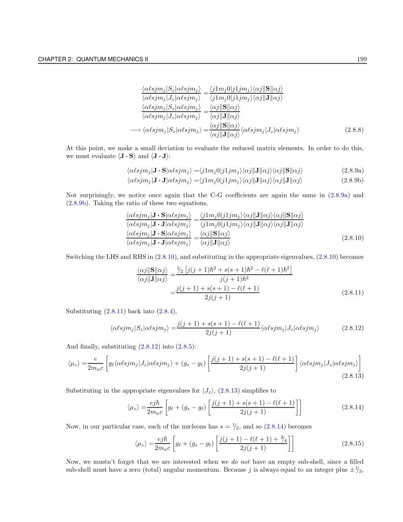
CHAPTER 2: QUANTUM MECHANICS II 199
〈α`sjmj |Sz|α`sjmj 〉〈α`sjmj |Jz|α`sjmj〉
=〈j1mj0|j1jmj〉〈αj‖S‖αj〉〈j1mj0|j1jmj〉〈αj‖J‖αj〉
〈α`sjmj |Sz|α`sjmj 〉〈α`sjmj |Jz|α`sjmj〉
=〈αj‖S‖αj〉〈αj‖J‖αj〉
−→ 〈α`sjmj |Sz|α`sjmj 〉 =〈αj‖S‖αj〉〈αj‖J‖αj〉 〈α`sjmj |Jz|α`sjmj〉 (2.8.8)
At this point, we make a small deviation to evaluate the reduced matrix elements. In order to do this,we must evaluate 〈J · S〉 and 〈J · J〉:
〈α`sjmj |J · S|α`sjmj〉 =〈j1mj0|j1jmj〉〈αj‖J‖αj〉〈αj‖S‖αj〉 (2.8.9a)
〈α`sjmj |J · J|α`sjmj〉 =〈j1mj0|j1jmj〉〈αj‖J‖αj〉〈αj‖J‖αj〉 (2.8.9b)
Not surprisingly, we notice once again that the C-G coefficients are again the same in (2.8.9a) and(2.8.9b). Taking the ratio of these two equations,
〈α`sjmj |J · S|α`sjmj〉〈α`sjmj |J · J|α`sjmj〉
=〈j1mj0|j1jmj〉〈αj‖J‖αj〉〈αj‖S‖αj〉〈j1mj0|j1jmj〉〈αj‖J‖αj〉〈αj‖J‖αj〉
〈α`sjmj |J · S|α`sjmj〉〈α`sjmj |J · J|α`sjmj〉
=〈αj‖S‖αj〉〈αj‖J‖αj〉 (2.8.10)
Switching the LHS and RHS in (2.8.10), and substituting in the appropriate eigenvalues, (2.8.10) becomes
〈αj‖S‖αj〉〈αj‖J‖αj〉 =
1/2[j(j + 1)~2 + s(s + 1)~2 − `(` + 1)~2
]
j(j + 1)~2
=j(j + 1) + s(s+ 1) − `(` + 1)
2j(j + 1)(2.8.11)
Substituting (2.8.11) back into (2.8.4),
〈α`sjmj |Sz|α`sjmj〉 =j(j + 1) + s(s+ 1) − `(` + 1)
2j(j + 1)〈α`sjmj |Jz|α`sjmj〉 (2.8.12)
And finally, substituting (2.8.12) into (2.8.5):
〈µz〉 =e
2mnc
[g`〈α`sjmj |Jz|α`sjmj 〉 + (gs − g`)
[j(j + 1) + s(s + 1) − `(` + 1)
2j(j + 1)
]〈α`sjmj |Jz|α`sjmj〉
]
(2.8.13)
Substituting in the appropriate eigenvalues for 〈Jz〉, (2.8.13) simplifies to
〈µz〉 =ej~
2mnc
[g` + (gs − g`)
[j(j + 1) + s(s+ 1) − `(` + 1)
2j(j + 1)
]](2.8.14)
Now, in our particular case, each of the nucleons has s = 1/2, and so (2.8.14) becomes
〈µz〉 =ej~
2mnc
[g` + (gs − g`)
[j(j + 1) − `(` + 1) + 3/4
2j(j + 1)
]](2.8.15)
Now, we mustn’t forget that we are interested when we do not have an empty sub-shell, since a filledsub-shell must have a zero (total) angular momentum. Because j is always equal to an integer plus ±1/2,
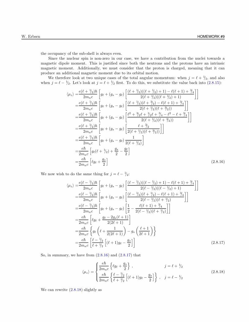
W. Erbsen HOMEWORK #9
the occupancy of the sub-shell is always even.Since the nuclear spin is non-zero in our case, we have a contribution from the nuclei towards a
magnetic dipole moment. This is justified since both the neutrons and the protons have an intrinsicmagnetic moment. Additionally, we must consider that the proton is charged, meaning that it canproduce an additional magnetic moment due to its orbital motion.
We therefore look at two unique cases of the total angular momentum: when j = ` + 1/2, and alsowhen j = ` − 1/2. Let’s look at j = `+ 1/2 first. To do this, we substitute the value back into (2.8.15):
〈µz〉 =e(` + 1/2)~
2mnc
[g` + (gs − g`)
[(` + 1/2)((` + 1/2) + 1) − `(` + 1) + 3/4
2(`+ 1/2)((` + 1/2) + 1)
]]
=e(` + 1/2)~
2mnc
[g` + (gs − g`)
[(` + 1/2)(` + 3/2) − `(` + 1) + 3/4
2(`+ 1/2)(` + 3/2))
]]
=e(` + 1/2)~
2mnc
[g` + (gs − g`)
[`2 + 3/2`+ 1/2` + 3/4 − `2 − ` + 3/4
2(` + 1/2)(` + 3/2))
]]
=e(` + 1/2)~
2mnc
[g` + (gs − g`)
[`+ 3/2
2(` + 1/2)(` + 3/2))
]]
=e(` + 1/2)~
2mnc
[g` + (gs − g`)
1
2(` + 1/2)
]
=e~
2mnc
[g`(` + 1/2) +
gs
2− g`
2
]
=e~
2mnc
[`g` +
gs
2
](2.8.16)
We now wish to do the same thing for j = `− 1/2:
〈µz〉 =e(` − 1/2)~
2mnc
[g` + (gs − g`)
[(` − 1/2)((` − 1/2) + 1) − `(` + 1) + 3/4
2(`− 1/2)((` − 1/2) + 1)
]]
=e(` − 1/2)~
2mnc
[g` + (gs − g`)
[(` − 1/2)(` + 1/2) − `(` + 1) + 3/4
2(`− 1/2)(` + 1/2)
]]
=e(` − 1/2)~
2mnc
[g` + (gs − g`)
[1
2− `(` + 1) + 3/4
2(`− 1/2)(` + 1/2)
]]
=e~
2mnc
[`g` +
g` − 2gs(` + 1)
2(2`+ 1)
]
=e~
2mnc
g`
(` +
1
2(2` + 1)
)− gs
(`+ 1
2`+ 1
)
=e~
2mnc
[`− 1/2`+ 1/2
[(` + 1)g` −
gs
2
]](2.8.17)
So, in summary, we have from (2.8.16) and (2.8.17) that
〈µz〉 =
e~
2mnc
`g` +
gs
2
, j = `+ 1/2
e~
2mnc
` − 1/2` + 1/2
[(` + 1)g` −
gs
2
], j = `− 1/2
(2.8.18)
We can rewrite (2.8.18) slightly as
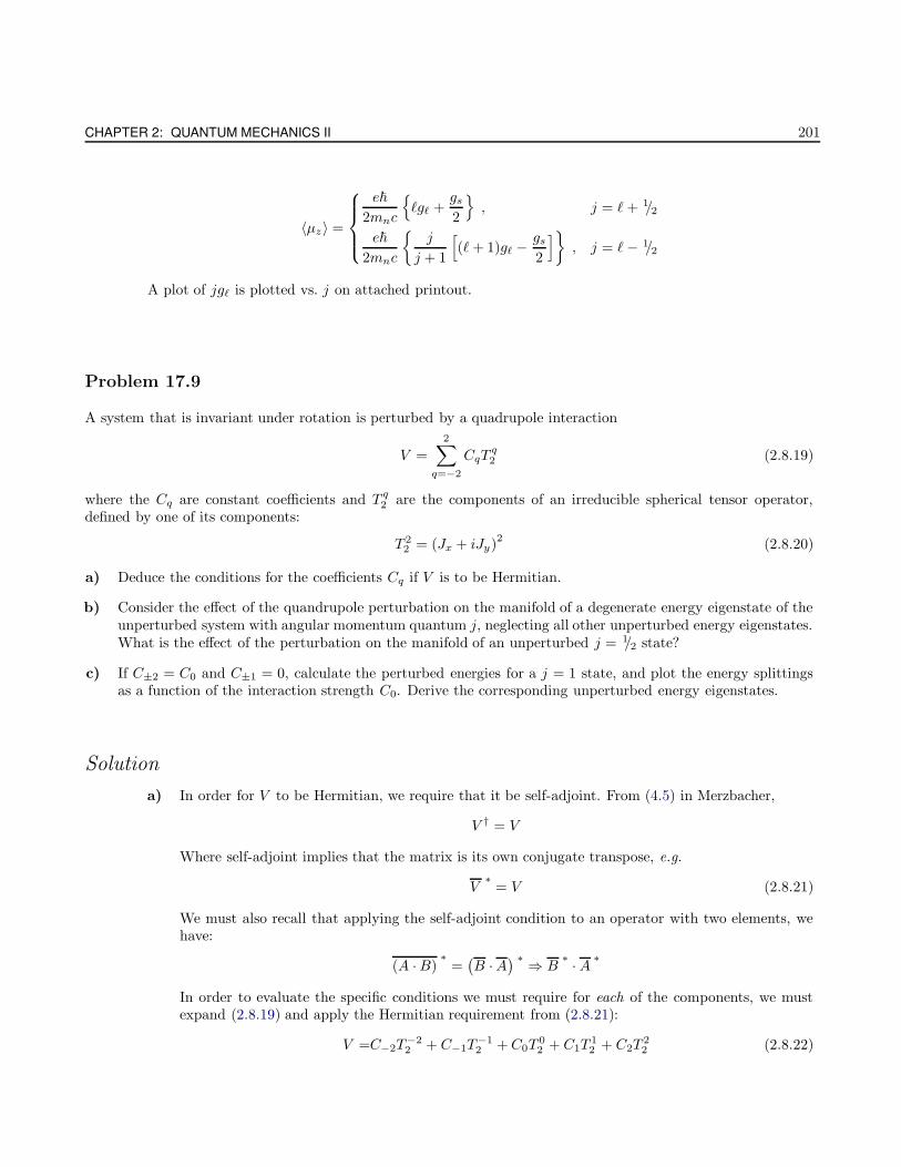
CHAPTER 2: QUANTUM MECHANICS II 201
〈µz〉 =
e~
2mnc
`g` +
gs
2
, j = ` + 1/2
e~
2mnc
j
j + 1
[(` + 1)g` −
gs
2
], j = ` − 1/2
A plot of jg` is plotted vs. j on attached printout.
Problem 17.9
A system that is invariant under rotation is perturbed by a quadrupole interaction
V =
2∑
q=−2
CqTq2 (2.8.19)
where the Cq are constant coefficients and T q2 are the components of an irreducible spherical tensor operator,
defined by one of its components:
T 22 = (Jx + iJy)
2(2.8.20)
a) Deduce the conditions for the coefficients Cq if V is to be Hermitian.
b) Consider the effect of the quandrupole perturbation on the manifold of a degenerate energy eigenstate of theunperturbed system with angular momentum quantum j, neglecting all other unperturbed energy eigenstates.What is the effect of the perturbation on the manifold of an unperturbed j = 1/2 state?
c) If C±2 = C0 and C±1 = 0, calculate the perturbed energies for a j = 1 state, and plot the energy splittingsas a function of the interaction strength C0. Derive the corresponding unperturbed energy eigenstates.
Solution
a) In order for V to be Hermitian, we require that it be self-adjoint. From (4.5) in Merzbacher,
V † = V
Where self-adjoint implies that the matrix is its own conjugate transpose, e.g.
V∗
= V (2.8.21)
We must also recall that applying the self-adjoint condition to an operator with two elements, wehave:
(A ·B)∗
=(B ·A
) ∗ ⇒ B∗ · A ∗
In order to evaluate the specific conditions we must require for each of the components, we mustexpand (2.8.19) and apply the Hermitian requirement from (2.8.21):
V =C−2T−22 + C−1T
−12 +C0T
02 + C1T
12 + C2T
22 (2.8.22)
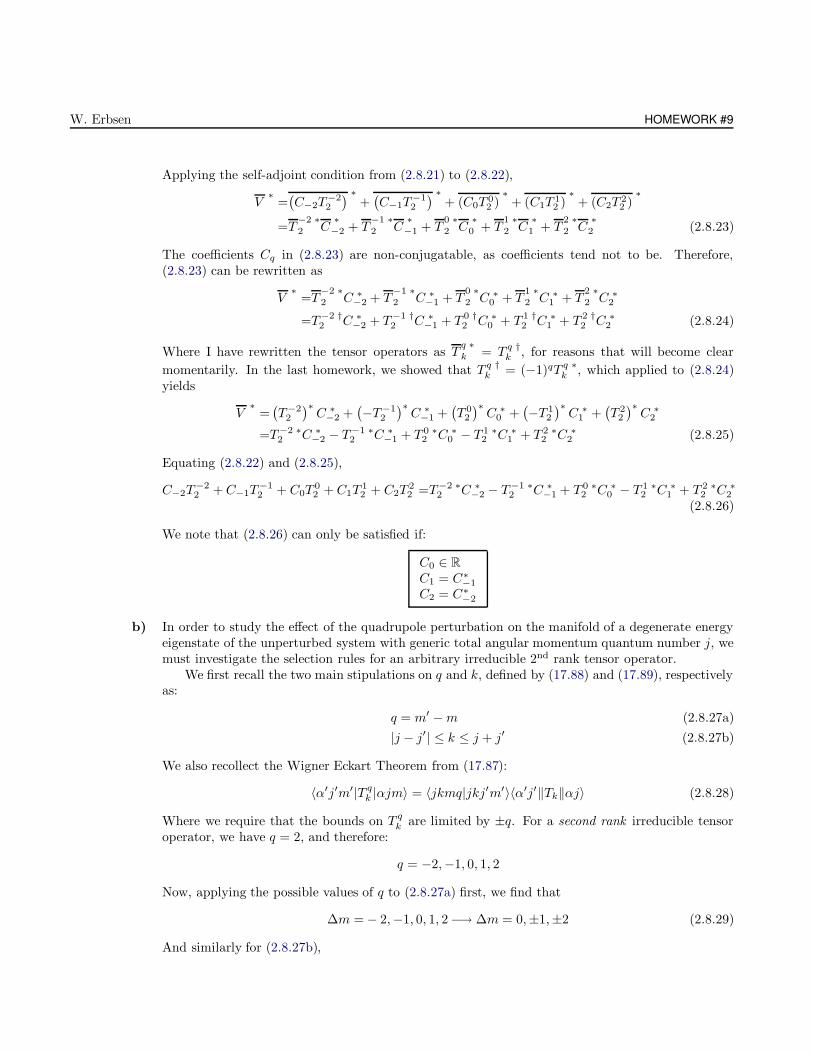
W. Erbsen HOMEWORK #9
Applying the self-adjoint condition from (2.8.21) to (2.8.22),
V∗
=(C−2T
−22
) ∗+(C−1T
−12
) ∗+ (C0T 0
2 )∗
+ (C1T 12 )
∗+ (C2T 2
2 )∗
=T−2 ∗2 C
∗−2 + T
−1 ∗2 C
∗−1 + T
0 ∗2 C
∗0 + T
1 ∗2 C
∗1 + T
2 ∗2 C
∗2 (2.8.23)
The coefficients Cq in (2.8.23) are non-conjugatable, as coefficients tend not to be. Therefore,(2.8.23) can be rewritten as
V∗
=T−2 ∗2 C ∗
−2 + T−1 ∗2 C ∗
−1 + T0 ∗2 C ∗
0 + T1 ∗2 C ∗
1 + T2 ∗2 C ∗
2
=T−2 †2 C ∗
−2 + T−1 †2 C ∗
−1 + T 0 †2 C ∗
0 + T 1 †2 C ∗
1 + T 2 †2 C ∗
2 (2.8.24)
Where I have rewritten the tensor operators as Tq ∗k = T q †
k , for reasons that will become clear
momentarily. In the last homework, we showed that T q †k = (−1)qT q ∗
k , which applied to (2.8.24)yields
V∗
=(T−2
2
)∗C ∗
−2 +(−T−1
2
)∗C ∗
−1 +(T 0
2
)∗C ∗
0 +(−T 1
2
)∗C ∗
1 +(T 2
2
)∗C ∗
2
=T−2 ∗2 C ∗
−2 − T−1 ∗2 C ∗
−1 + T 0 ∗2 C ∗
0 − T 1 ∗2 C ∗
1 + T 2 ∗2 C ∗
2 (2.8.25)
Equating (2.8.22) and (2.8.25),
C−2T−22 +C−1T
−12 + C0T
02 +C1T
12 + C2T
22 =T−2 ∗
2 C ∗−2 − T−1 ∗
2 C ∗−1 + T 0 ∗
2 C ∗0 − T 1 ∗
2 C ∗1 + T 2 ∗
2 C ∗2
(2.8.26)
We note that (2.8.26) can only be satisfied if:
C0 ∈ R
C1 = C∗−1
C2 = C∗−2
b) In order to study the effect of the quadrupole perturbation on the manifold of a degenerate energyeigenstate of the unperturbed system with generic total angular momentum quantum number j, wemust investigate the selection rules for an arbitrary irreducible 2nd rank tensor operator.
We first recall the two main stipulations on q and k, defined by (17.88) and (17.89), respectivelyas:
q = m′ −m (2.8.27a)
|j − j′| ≤ k ≤ j + j′ (2.8.27b)
We also recollect the Wigner Eckart Theorem from (17.87):
〈α′j′m′|T qk |αjm〉 = 〈jkmq|jkj′m′〉〈α′j′‖Tk‖αj〉 (2.8.28)
Where we require that the bounds on T qk are limited by ±q. For a second rank irreducible tensor
operator, we have q = 2, and therefore:
q = −2,−1, 0, 1, 2
Now, applying the possible values of q to (2.8.27a) first, we find that
∆m = − 2,−1, 0, 1, 2−→ ∆m = 0,±1,±2 (2.8.29)
And similarly for (2.8.27b),
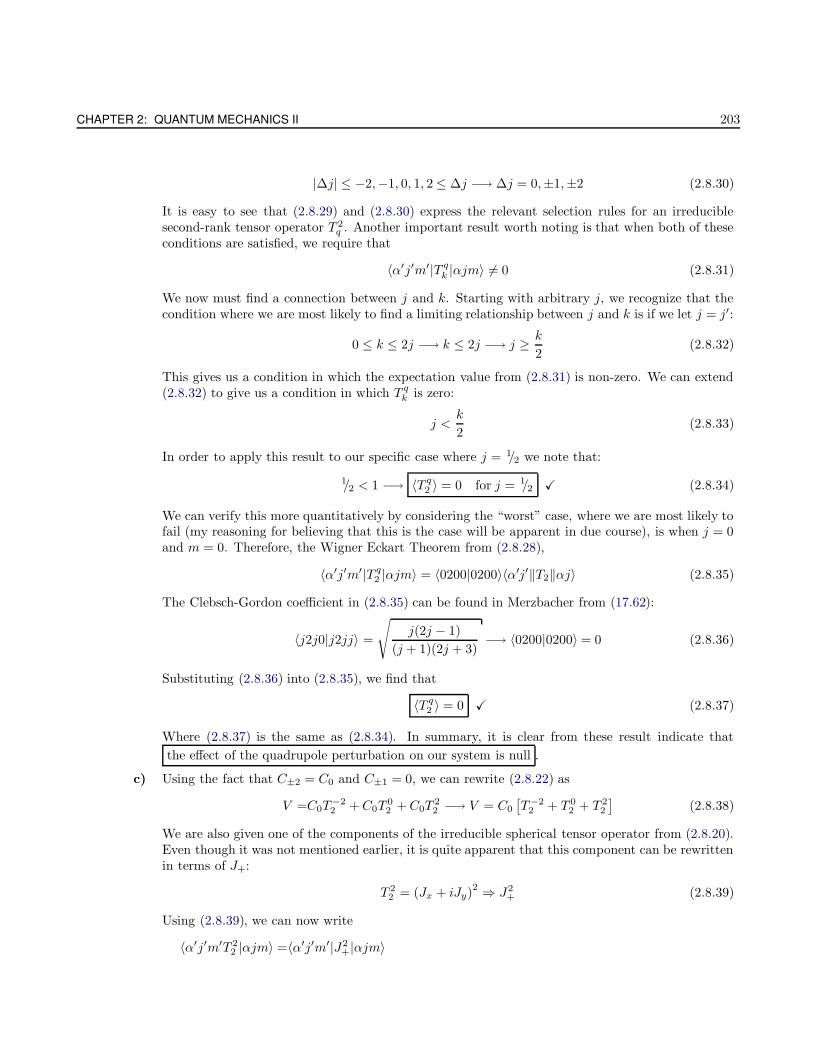
CHAPTER 2: QUANTUM MECHANICS II 203
|∆j| ≤ −2,−1, 0, 1, 2 ≤ ∆j −→ ∆j = 0,±1,±2 (2.8.30)
It is easy to see that (2.8.29) and (2.8.30) express the relevant selection rules for an irreduciblesecond-rank tensor operator T 2
q . Another important result worth noting is that when both of theseconditions are satisfied, we require that
〈α′j′m′|T qk |αjm〉 6= 0 (2.8.31)
We now must find a connection between j and k. Starting with arbitrary j, we recognize that thecondition where we are most likely to find a limiting relationship between j and k is if we let j = j′:
0 ≤ k ≤ 2j −→ k ≤ 2j −→ j ≥ k
2(2.8.32)
This gives us a condition in which the expectation value from (2.8.31) is non-zero. We can extend(2.8.32) to give us a condition in which T q
k is zero:
j <k
2(2.8.33)
In order to apply this result to our specific case where j = 1/2 we note that:
1/2 < 1 −→ 〈T q2 〉 = 0 for j = 1/2 X (2.8.34)
We can verify this more quantitatively by considering the “worst” case, where we are most likely tofail (my reasoning for believing that this is the case will be apparent in due course), is when j = 0and m = 0. Therefore, the Wigner Eckart Theorem from (2.8.28),
〈α′j′m′|T q2 |αjm〉 = 〈0200|0200〉〈α′j′‖T2‖αj〉 (2.8.35)
The Clebsch-Gordon coefficient in (2.8.35) can be found in Merzbacher from (17.62):
〈j2j0|j2jj〉 =
√j(2j − 1)
(j + 1)(2j + 3)−→ 〈0200|0200〉 = 0 (2.8.36)
Substituting (2.8.36) into (2.8.35), we find that
〈T q2 〉 = 0 X (2.8.37)
Where (2.8.37) is the same as (2.8.34). In summary, it is clear from these result indicate that
the effect of the quadrupole perturbation on our system is null .
c) Using the fact that C±2 = C0 and C±1 = 0, we can rewrite (2.8.22) as
V =C0T−22 +C0T
02 +C0T
22 −→ V = C0
[T−2
2 + T 02 + T 2
2
](2.8.38)
We are also given one of the components of the irreducible spherical tensor operator from (2.8.20).Even though it was not mentioned earlier, it is quite apparent that this component can be rewrittenin terms of J+:
T 22 = (Jx + iJy)
2 ⇒ J2+ (2.8.39)
Using (2.8.39), we can now write
〈α′j′m′T 22 |αjm〉 =〈α′j′m′|J2
+|αjm〉
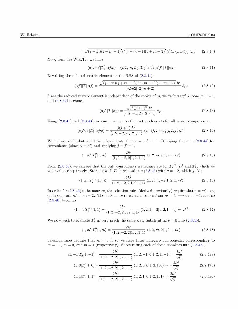
W. Erbsen HOMEWORK #9
=√
(j −m)(j +m+ 1)√
(j −m− 1)(j +m+ 2) ~2δm′,m+2δjj′δαα′ (2.8.40)
Now, from the W.E.T. , we have
〈α′j′m′|T 22 |αjm〉 =〈j, 2, m, 2|j, 2, j′, m′〉〈α′j′‖T‖αj〉 (2.8.41)
Rewriting the reduced matrix element on the RHS of (2.8.41),
〈αj′‖T‖αj〉 =
√(j −m)(j +m+ 1)(j −m− 1)(j +m+ 2) ~2
〈j2m2|j2jm + 2〉 δjj′ (2.8.42)
Since the reduced matrix element is independent of the choice of m, we “arbitrary” choose m = −1,and (2.8.42) becomes
〈αj′‖T‖αj〉 =
√j2(j + 1)2 ~2
〈j, 2,−1, 2|j, 2, j, 1〉 δjj′ (2.8.43)
Using (2.8.41) and (2.8.43), we can now express the matrix elements for all tensor components:
〈αj′m′|T q2 |αjm〉 =
j(j + 1) ~2
〈j, 2,−2, 2|j, 2, j, 1〉 δjj′ 〈j, 2, m, q|j, 2, j′, m′〉 (2.8.44)
Where we recall that selection rules dictate that q = m′ − m. Dropping the α in (2.8.44) forconvenience (since α = α′) and applying j = j′ = 1,
〈1, m′|T q2 |1, m〉 =
2~2
〈1, 2,−2, 2|1, 2, 1, 1〉 〈1, 2, m, q|1, 2, 1, m′〉 (2.8.45)
From (2.8.38), we can see that the only components we require are for T−22 , T 0
2 and T 22 , which we
will evaluate separately. Starting with T−22 , we evaluate (2.8.45) with q = −2, which yields
〈1, m′|T−22 |1, m〉 =
2~2
〈1, 2,−2, 2|1, 2, 1, 1〉 〈1, 2, m,−2|1, 2, 1,m′〉 (2.8.46)
In order for (2.8.46) to be nonzero, the selection rules (derived previously) require that q = m′ −m,or in our case m′ = m − 2. The only nonzero element comes from m = 1 −→ m′ = −1, and so(2.8.46) becomes
〈1,−1|T−22 |1, 1〉 =
2~2
〈1, 2,−2, 2|1, 2, 1, 1〉 〈1, 2, 1,−2|1, 2, 1,−1〉 ⇒ 2~2 (2.8.47)
We now wish to evaluate T 02 in very much the same way. Substituting q = 0 into (2.8.45),
〈1, m′|T 02 |1, m〉 =
2~2
〈1, 2,−2, 2|1, 2, 1, 1〉 〈1, 2, m, 0|1, 2, 1,m′〉 (2.8.48)
Selection rules require that m = m′, so we have three non-zero components, corresponding tom = −1, m = 0, and m = 1 (respectively). Substituting each of these m-values into (2.8.48),
〈1,−1|T 02 |1,−1〉 =
2~2
〈1, 2,−2, 2|1, 2, 1, 1〉 〈1, 2,−1, 0|1, 2, 1,−1〉 ⇒ 2~2
√6
(2.8.49a)
〈1, 0|T 02 |1, 0〉 =
2~2
〈1, 2,−2, 2|1, 2, 1, 1〉 〈1, 2, 0, 0|1, 2, 1, 0〉⇒ −4~2
√6
(2.8.49b)
〈1, 1|T 02 |1, 1〉 =
2~2
〈1, 2,−2, 2|1, 2, 1, 1〉 〈1, 2, 1, 0|1, 2, 1, 1〉⇒2~2
√6
(2.8.49c)
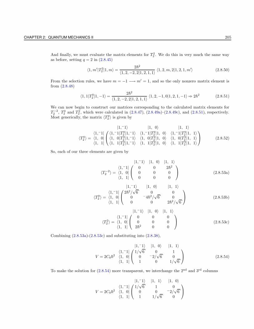
CHAPTER 2: QUANTUM MECHANICS II 205
And finally, we must evaluate the matrix elements for T 22 . We do this in very much the same way
as before, setting q = 2 in (2.8.45)
〈1, m′|T 22 |1, m〉 =
2~2
〈1, 2,−2, 2|1, 2, 1, 1〉 〈1, 2, m, 2|1, 2, 1,m′〉 (2.8.50)
From the selection rules, we have m = −1 −→ m′ = 1, and so the only nonzero matrix element isfrom (2.8.48)
〈1, 1|T 02 |1,−1〉 =
2~2
〈1, 2,−2, 2|1, 2, 1, 1〉 〈1, 2,−1, 0|1, 2, 1,−1〉 ⇒ 2~2 (2.8.51)
We can now begin to construct our matrices corresponding to the calculated matrix elements forT−2
2 , T 02 and T 2
2 , which were calculated in (2.8.47), (2.8.49a)–(2.8.49c), and (2.8.51), respectively.Most generically, the matrix 〈T q
2 〉 is given by
〈T q2 〉 =
|1,−1〉 |1, 0〉 |1, 1〉〈1,−1| 〈1,−1|T q
2 |1,−1〉 〈1,−1|T q2 |1, 0〉 〈1,−1|T q
2 |1, 1〉〈1, 0| 〈1, 0|T q
2 |1,−1〉 〈1, 0|T q2 |1, 0〉 〈1, 0|T q
2 |1, 1〉〈1, 1| 〈1, 1|T q
2 |1,−1〉 〈1, 1|T q2 |1, 0〉 〈1, 1|T q
2 |1, 1〉
(2.8.52)
So, each of our three elements are given by
〈T−22 〉 =
|1,−1〉 |1, 0〉 |1, 1〉〈1,−1| 0 0 2~2
〈1, 0| 0 0 0〈1, 1| 0 0 0
(2.8.53a)
〈T 02 〉 =
|1,−1〉 |1, 0〉 |1, 1〉〈1,−1| 2~2/
√6 0 0
〈1, 0| 0 −4~2/√
6 0〈1, 1| 0 0 2~2/
√6
(2.8.53b)
〈T 22 〉 =
|1,−1〉 |1, 0〉 |1, 1〉〈1,−1| 0 0 0〈1, 0| 0 0 0〈1, 1| 2~2 0 0
(2.8.53c)
Combining (2.8.53a)-(2.8.53c) and substituting into (2.8.38),
V = 2C0~2
|1,−1〉 |1, 0〉 |1, 1〉〈1,−1| 1/
√6 0 1
〈1, 0| 0 −2/√
6 0〈1, 1| 1 0 1/
√6
(2.8.54)
To make the solution for (2.8.54) more transparent, we interchange the 2nd and 3rd columns
V = 2C0~2
|1,−1〉 |1, 1〉 |1, 0〉〈1,−1| 1/
√6 1 0
〈1, 0| 0 0 −2/√
6〈1, 1| 1 1/
√6 0

W. Erbsen HOMEWORK #9
And now do the same thing for the 1st and 3rd rows,
V = 2C0~2
|1,−1〉 |1, 1〉 |1, 0〉〈1,−1| 1/
√6 1 0
〈1, 1| 1 1/√
6 0〈1, 0| 0 0 −2/
√6
(2.8.55)
It is easy to see that we needn’t diagonalize the entire matrix in (2.8.55); rather, only the 2 × 2submatrix:
V ′ = 2C0~2
( |1,−1〉 |1, 1〉〈1,−1| 1/
√6 1
〈1, 1| 1 1/√
6
)(2.8.56)
Diagonalizing (2.8.56), we find that∣∣∣∣
2C0~2/√
6 − λ 2C0~2
2C0~2 2C0~
2/√
6 − λ
∣∣∣∣ = 0 −→(
2C0~2
√6
− λ
)(2C0~
2
√6
− λ
)− 4C0~
2 = 0
−→λ2 − 4C0~2
√6
λ− 10C20~4
3= 0
−→λ = 2C0~2
(1√6
± 1
)(2.8.57)
Using (2.8.57), we can now find the corresponding eivenvectors. For λ = 2C0~2(
1√6
+ 1), we have
2C0~2
(−1 11 −1
)(|1, 1〉|1,− 1〉
)=
(00
)−→ N
(|1, 1〉 + |1,− 1〉
)= 0 (2.8.58)
And similarly, for λ = 2C0~2(
1√6− 1),
2C0~2
(1 11 1
)(|1, 1〉|1,− 1〉
)=
(00
)−→ N
(|1, 1〉 − |1,− 1〉
)= 0 (2.8.59)
Where the normalization constant N in (2.8.58) and (2.8.59) is simply 1/√
2 . The eigenvalues andeigenvectors are then
λ1 = − 4C0~2
√6
, |1, 0〉 = 0 (2.8.60)
λ2 =2C0~2
(1√6
+ 1
),
1√2
(|1, 1〉 + |1,− 1〉
)= 0 (2.8.61)
λ3 =2C0~2
(1√6
− 1
),
1√2
(|1, 1〉 − |1,− 1〉
)= 0 (2.8.62)
The eigenvalues in (2.8.60) are the energy shifts (∆E), while the eigenvectors correspond to theunperturbed energy Eigenstates. The energy shifts are plotted in Fig. (3) (see attached Mathamaticaprintout).
Exercise 21.4
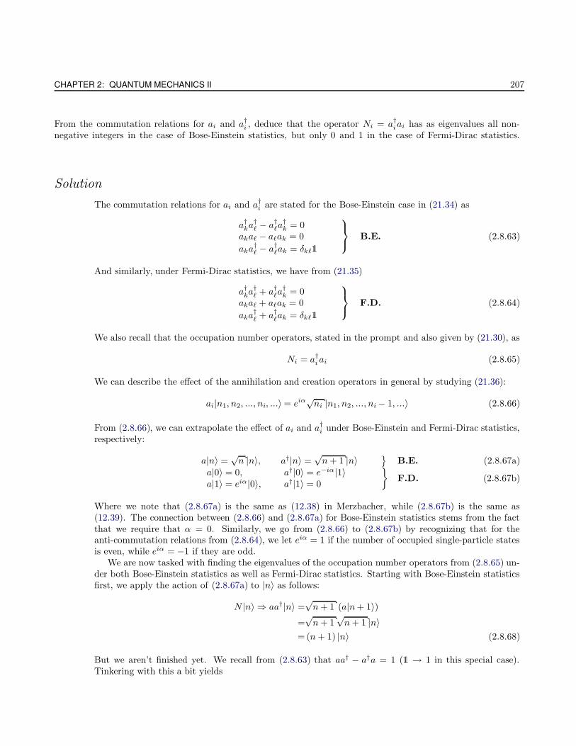
CHAPTER 2: QUANTUM MECHANICS II 207
From the commutation relations for ai and a†i , deduce that the operator Ni = a†iai has as eigenvalues all non-negative integers in the case of Bose-Einstein statistics, but only 0 and 1 in the case of Fermi-Dirac statistics.
Solution
The commutation relations for ai and a†i are stated for the Bose-Einstein case in (21.34) as
a†ka†` − a†`a
†k = 0
aka` − a`ak = 0
aka†` − a†`ak = δk`1
B.E. (2.8.63)
And similarly, under Fermi-Dirac statistics, we have from (21.35)
a†ka†` + a†`a
†k = 0
aka` + a`ak = 0
aka†` + a†`ak = δk`1
F.D. (2.8.64)
We also recall that the occupation number operators, stated in the prompt and also given by (21.30), as
Ni = a†iai (2.8.65)
We can describe the effect of the annihilation and creation operators in general by studying (21.36):
ai|n1, n2, ..., ni, ...〉 = eiα√ni |n1, n2, ..., ni − 1, ...〉 (2.8.66)
From (2.8.66), we can extrapolate the effect of ai and a†i under Bose-Einstein and Fermi-Dirac statistics,respectively:
a|n〉 =√n |n〉, a†|n〉 =
√n+ 1 |n〉
B.E. (2.8.67a)
a|0〉 = 0, a†|0〉 = e−iα|1〉a|1〉 = eiα|0〉, a†|1〉 = 0
F.D. (2.8.67b)
Where we note that (2.8.67a) is the same as (12.38) in Merzbacher, while (2.8.67b) is the same as(12.39). The connection between (2.8.66) and (2.8.67a) for Bose-Einstein statistics stems from the factthat we require that α = 0. Similarly, we go from (2.8.66) to (2.8.67b) by recognizing that for theanti-commutation relations from (2.8.64), we let eiα = 1 if the number of occupied single-particle statesis even, while eiα = −1 if they are odd.
We are now tasked with finding the eigenvalues of the occupation number operators from (2.8.65) un-der both Bose-Einstein statistics as well as Fermi-Dirac statistics. Starting with Bose-Einstein statisticsfirst, we apply the action of (2.8.67a) to |n〉 as follows:
N |n〉 ⇒ aa†|n〉 =√n+ 1 (a|n+ 1〉)
=√n+ 1
√n+ 1 |n〉
=(n+ 1) |n〉 (2.8.68)
But we aren’t finished yet. We recall from (2.8.63) that aa† − a†a = 1 (1 → 1 in this special case).Tinkering with this a bit yields
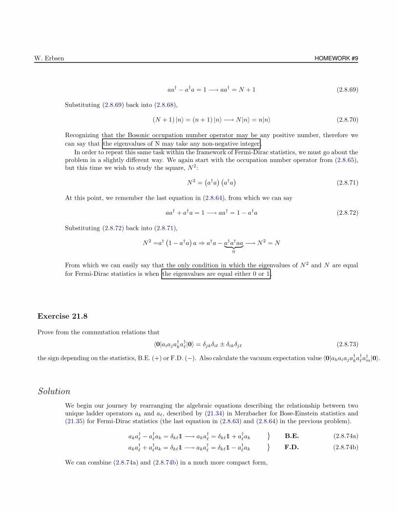
W. Erbsen HOMEWORK #9
aa† − a†a = 1 −→ aa† = N + 1 (2.8.69)
Substituting (2.8.69) back into (2.8.68),
(N + 1) |n〉 = (n+ 1) |n〉 −→ N |n〉 = n|n〉 (2.8.70)
Recognizing that the Bosonic occupation number operator may be any positive number, therefore we
can say that the eigenvalues of N may take any non-negative integer .
In order to repeat this same task within the framework of Fermi-Dirac statistics, we must go about theproblem in a slightly different way. We again start with the occupation number operator from (2.8.65),but this time we wish to study the square, N2:
N2 =(a†a) (a†a)
(2.8.71)
At this point, we remember the last equation in (2.8.64), from which we can say
aa† + a†a = 1 −→ aa† = 1 − a†a (2.8.72)
Substituting (2.8.72) back into (2.8.71),
N2 =a†(1 − a†a
)a ⇒ a†a− a†a†aa︸ ︷︷ ︸
0
−→ N2 = N
From which we can easily say that the only condition in which the eigenvalues of N2 and N are equal
for Fermi-Dirac statistics is when the eigenvalues are equal either 0 or 1 .
Exercise 21.8
Prove from the commutation relations that
〈0|aiaja†ka
†`|0〉 = δjkδi` ± δikδj` (2.8.73)
the sign depending on the statistics, B.E. (+) or F.D. (−). Also calculate the vacuum expectation value 〈0|ahaiaja†ka
†`a
†m|0〉.
Solution
We begin our journey by rearranging the algebraic equations describing the relationship between twounique ladder operators ak and a`, described by (21.34) in Merzbacher for Bose-Einstein statistics and(21.35) for Fermi-Dirac statistics (the last equation in (2.8.63) and (2.8.64) in the previous problem).
aka†` − a†`ak = δk`1 −→ aka
†` = δk`1 + a†`ak
B.E. (2.8.74a)
aka†` + a†`ak = δk`1 −→ aka
†` = δk`1− a†`ak
F.D. (2.8.74b)
We can combine (2.8.74a) and (2.8.74b) in a much more compact form,
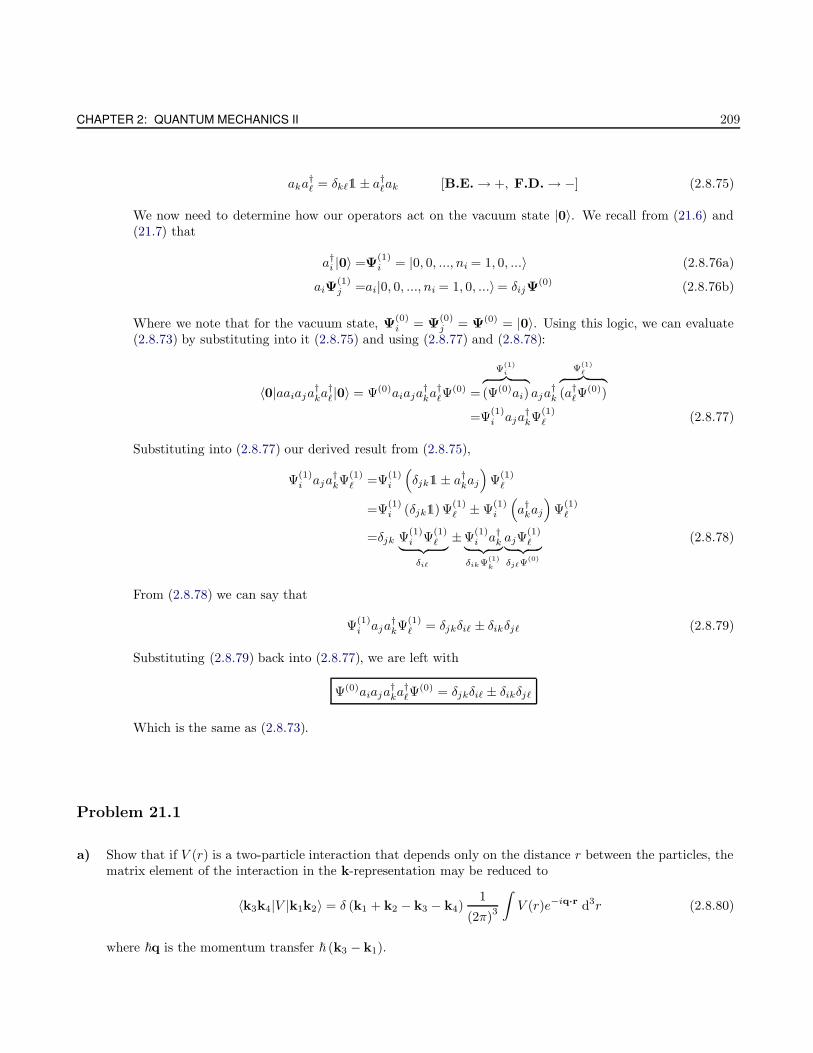
CHAPTER 2: QUANTUM MECHANICS II 209
aka†` = δk`1± a†`ak [B.E. → +, F.D. → −] (2.8.75)
We now need to determine how our operators act on the vacuum state |0〉. We recall from (21.6) and(21.7) that
a†i |0〉 =Ψ(1)i = |0, 0, ..., ni = 1, 0, ...〉 (2.8.76a)
aiΨ(1)j =ai|0, 0, ..., ni = 1, 0, ...〉= δijΨ
(0) (2.8.76b)
Where we note that for the vacuum state, Ψ(0)i = Ψ
(0)j = Ψ(0) = |0〉. Using this logic, we can evaluate
(2.8.73) by substituting into it (2.8.75) and using (2.8.77) and (2.8.78):
〈0|aaiaja†ka
†`|0〉 = Ψ(0)aiaja
†ka
†`Ψ
(0) =
Ψ(1)i︷ ︸︸ ︷
(Ψ(0)ai) aja†k
Ψ(1)`︷ ︸︸ ︷
(a†`Ψ(0))
=Ψ(1)i aja
†kΨ
(1)` (2.8.77)
Substituting into (2.8.77) our derived result from (2.8.75),
Ψ(1)i aja
†kΨ
(1)` =Ψ
(1)i
(δjk1± a†kaj
)Ψ
(1)`
=Ψ(1)i (δjk1)Ψ
(1)` ± Ψ
(1)i
(a†kaj
)Ψ
(1)`
=δjk Ψ(1)i Ψ
(1)`︸ ︷︷ ︸
δi`
±Ψ(1)i a†k︸ ︷︷ ︸
δikΨ(1)k
ajΨ(1)`︸ ︷︷ ︸
δj`Ψ(0)
(2.8.78)
From (2.8.78) we can say that
Ψ(1)i aja
†kΨ
(1)` = δjkδi` ± δikδj` (2.8.79)
Substituting (2.8.79) back into (2.8.77), we are left with
Ψ(0)aiaja†ka
†`Ψ
(0) = δjkδi` ± δikδj`
Which is the same as (2.8.73).
Problem 21.1
a) Show that if V (r) is a two-particle interaction that depends only on the distance r between the particles, thematrix element of the interaction in the k-representation may be reduced to
〈k3k4|V |k1k2〉 = δ (k1 + k2 − k3 − k4)1
(2π)3
∫V (r)e−iq·r d3r (2.8.80)
where ~q is the momentum transfer ~ (k3 − k1).
W. Erbsen HOMEWORK #9
b) For this interaction, show that the mutual potential energy operator is
V =1
2
∫∫∫φ† (k1 + q)φ† (k2 − q) φ (k2)φ (k1)F (q) d3k1 d3k2 d3q (2.8.81)
where F (q) is the Fourier transform of the displacement-invariant interaction.
Solution
Before we get down to business, we must lay down some formalism. We recall that within the frameworkof identical particles, ai and a†i destroy and create particles with some quantum numberKi. We also recallthat L represents a complete set of one-particle observables, whose eigenvalues are Lq . The relationshipbetween Ki and Lq is given by (21.9) as
|Ki〉 =∑
q
|Lq〉〈Lq |Ki〉 (2.8.82)
We can also evaluate the expectation value of K by expanding it in terms of Ki:
〈Lq |K|Lr〉 =∑
i
〈Lq|Ki〉Ki〈Ki|Lr〉 (2.8.83)
Which is of course (21.43). We also wish to define an additive two-particle operator as
V =1
2
∑
ij
a†ia†jajai Vij ⇒ 1
2
∑
qrst
b†qb†rbsbt 〈qr|V |ts〉 (2.8.84)
Where, from (21.48),
〈qr|V |st〉 =∑
ij
〈Lq |Ki〉〈Ki|Lt〉〈Lr |Kj〉〈Kj |Ls〉 Vij (2.8.85)
We note that (2.8.85) is the generalized two-particle matrix element, and according to Merzbacher’schosen convention we require that r and s belong to one particle, while q and t to the other. We alsorecall the following symmetry property:
〈qr|V |ts〉 = 〈rq|V |st〉
Which should come as no surprise.
a) We are now tasked with finding the two-particle matrix element in the k-representation. The mostgeneral form is given by (2.8.85), and we note that since our interaction stems from a mutualpotential energy, (2.8.84) and (2.8.85) can be readily used.
The first thing we wish to do is rewrite our k-representation two-particle matrix element fromthe LHS of (2.8.80) in terms of the more generic form of (2.8.85):
〈k3k4|V |k1k2〉 =∑
ij
〈k3|ri〉〈ri|k1〉〈k4|rj〉〈rj |k2〉 Vij (2.8.86)
Our particle coordinates are r1 and r2, while the interaction potential between the two particles isonly dependent on the distance between them (call this distance r), so that Vij = V (r1−r2) = V (r).Accordingly, (2.8.86) becomes
CHAPTER 2: QUANTUM MECHANICS II 211
〈k3k4|V |k1k2〉 =∑
12
〈k3|r1〉〈r1|k1〉〈k4|r2〉〈r2|k2〉 V (r) (2.8.87)
It is very important that we recognize that the summation indicies in (2.8.87) are referring to thecoordinates r1 and r2, and mustn’t be applied to k. Since r1 and r2 are continuous variables, wemay take the sums in (2.8.87) to be integrals. We now have
〈k3k4|V |k1k2〉 =
∫∫〈k3|r1〉〈r1|k1〉〈k4|r2〉〈r2|k2〉 V (r) d3r1d
3r2 (2.8.88)
At this point, we wish to reexpress (2.8.88) in terms of momentum eigenstates, which we will do inthe usual way. Most generally,
Ψ(r) =〈r
1 =
∫|k〉〈k| dk
↓|Ψ〉
=
∫〈r|k〉〈k|Ψ〉 dk (2.8.89)
We also recall that (〈k|r〉)∗ = 〈r|k〉 ⇒ Ne−ik·r/~, while normalizing this yields
|N |2∫ ∞
−∞eik·(r−r′)/~ −→ N =
1√2π~
, < δ (r − r′) (2.8.90)
Compensating for the fact that dr → d3r, we can now say that
〈r|k〉 =1
(2π~)3/2eik·r/~ (2.8.91)
We now rewrite (2.8.88) in a slightly more transparent way,
〈k3k4|V |k1k2〉 =
∫∫〈r1|k3〉∗〈r1|k1〉 〈r2|k4〉∗〈r2|k2〉 V (r) d3r1d
3r2 (2.8.92)
We can now evaluate each of the coefficients in (2.8.93) by applying (2.8.91):
〈r1|k3〉∗ =1
(2π~)3/2e−ik3·r1/~
〈r1|k1〉 =1
(2π~)3/2eik1·r1/~
〈r2|k4〉∗ =1
(2π~)3/2e−ik4·r2/~
〈r2|k2〉 =1
(2π~)3/2eik2·r2/~
And substituting these into (2.8.93),
〈k3k4|V |k1k2〉 =1
(2π~)6
∫∫exp
[i
~(−k3 · r1 + k1 · r1 − k4 · r2 + k2 · r2)
]V (r) d3r1d
3r2
(2.8.93)
By substituting r = r1 − r2 −→ r1 = r2 + r into (2.8.93) and completing the square, we arrive at
W. Erbsen HOMEWORK #9
〈k3k4|V |k1k2〉 =
∫e−iq·r2e−i(k4−k2)·r2 d3r2
eiq·r2
∫V (r)e−iq·r1 d3r1 − eiq·r1
∫V (r)eiq·r2 d3r2
=1
(2π~)3
∫ei(k1+k2−k3−k4)·r2/~ d3r2
∫V (r)e−iq·r/~ d3r (2.8.94)
Noticing that the first integral in (2.8.94) is a δ-function, we are left with
〈k3k4|V |k1k2〉 = δ (k1 + k2 − k3 − k4)1
(2π)3
∫V (r)e−iq·r d3r
Problem 21.2
Show that the diagonal part of the interaction operator V , found in Problem 1 in the k-representation, arisesfrom momentum transfers q = 0 and q = k2 −k1, respectively. Write down the two interaction terms and identifythem as direct (q = 0) and exchange (q = k2 −k1) interactions. Draw the corresponding diagrams (Figure 21.1).
Solution
We first recall from (21.51) that
ψσ′ (r′)ψσ′′ (r′′) − ψσ′′ (r′′)ψσ′ (r′) = 0
ψ†σ′ (r′)ψ
†σ′′ (r′′) − ψ†
σ′′ (r′′)ψ†σ′ (r′) = 0
ψσ′ (r′)ψ†σ′′ (r′′) − ψ†
σ′′ (r′′)ψσ′ (r′) = δ(r′ − r′′) δσ′σ′′
B.E. (2.8.95)
And similarly, under Fermi-Dirac statistics, we have from (21.52)
ψσ′ (r′)ψσ′′ (r′′) + ψσ′′ (r′′)ψσ′ (r′) = 0
ψ†σ′ (r′)ψ
†σ′′ (r′′) + ψ†
σ′′ (r′′)ψ†σ′ (r′) = 0
ψσ′ (r′)ψ†σ′′ (r′′) + ψ†
σ′′ (r′′)ψσ′ (r′) = δ(r′ − r′′) δσ′σ′′
F.D. (2.8.96)
We also recall from (21.53) that
N =∑
σ′
∫ψ†
σ′ (r′)ψσ′ (r′) d3r′ (2.8.97)
From the previous problem, we have
V =1
2
∫∫∫φ† (k1 + q)φ† (k2 − q)φ (k2)φ (k1)F (q) d3k1 d3k2 d3q (2.8.98)
Substituting in to (2.8.98) the appropriate value for q and simplifying, we have
V =1
2
∫∫∫∫φ†(k3)φ
†(k4)φ(k2)φ(k1)〈k3k4|k2k1〉 d3k1d3k2d
3k3d3k4 (2.8.99)
We now wish to sandwich (2.8.99) between the state ψn as follows:
CHAPTER 2: QUANTUM MECHANICS II 213
〈ψn|V |ψn〉 =1
2
∫∫∫∫〈ψn|φ†(k3)φ
†(k4)φ(k2)φ(k1)|ψn〉〈k3k4|k2k1〉 d3k1d3k2d
3k3d3k4 (2.8.100)
The generic interaction term we are interested in is given from (2.8.100) as
〈ψn|φ†(k3)φ†(k4)φ(k2)φ(k1)|ψn〉 (2.8.101)
Now, if q = 0, then we require from the prompt that k1 = k3 and k2 = k4, and so (2.8.101) becomes
〈ψn|φ†(k1)φ†(k2)φ(k2)φ(k1)|ψn〉 =〈ψn |φ†(k1)φ(k1)φ
†(k2)φ(k2)|ψn〉 (2.8.102)
Where we recall that the number operator acts like Ni = a†iai. Accordingly, if we recall that Niψ = niψ,from (2.8.102) we have
〈ψn |φ†(k1)φ(k1)φ†(k2)φ(k2)|ψn〉 =n1n2 (2.8.103)
If, on the other hand, q = 0 because k1 = k2 = k3 = k4 ⇒ k, then
〈ψn |φ†(k1)φ†(k2)φ(k2)φ(k1)|ψn〉 =〈ψn|φ†(k)φ(k)φ†(k)φ(k)|ψn〉
=〈ψn|φ†(k)φ†(k)φ(k)φ(k)|ψn〉=〈ψn|φ†(k)φ†(k)φ(k)φ(k)|ψn〉 (2.8.104)
The result of (2.8.104) is not the same for each flavor of particles; for symmetric particles, the RHS of(2.8.104) is n(n− 1), and for anti-symmetric particles, it is equal to 0, which comes as no surprise.
Following the same logic, we have for q 6= 0 that k3 = k2 and k1 = k4. The number operators actas before, and we end up with
〈ψn|φ†(k1)φ(k1)φ†(k2)φ(k2)|ψn〉 =〈ψn |φ†(k1)φ(k1)φ
†(k2)φ(k2)|ψn〉⇒A n1n2 (2.8.105)
Where for symmetric particles, A = 1, and for anti-symmetric particles A = −1. We finally can say that
the “direct” terms come from q = 0 , while the “exchange terms” come from q = k1 − k2 . Please see
diagrams in Fig. (4) and (5) (attached at the end of this assignment).
2.9 Homework #10
Exercise 22.3
Construct explicitly in terms of the states of the form a†jm2αa†jm1α |0〉 the total angular momentum eigenstates for
two neutrons in the configurations (p1/2)2 and (p3/2)
2. How would the angular momentum eigenstates look if thetwo particles were a neutron and a proton but otherwise had the same quantum numbers as before?
Solution
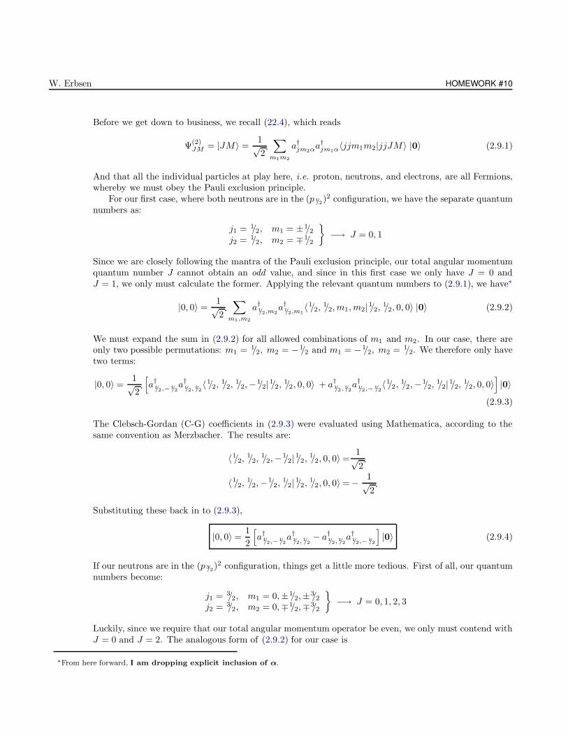
W. Erbsen HOMEWORK #10
Before we get down to business, we recall (22.4), which reads
Ψ(2)JM = |JM〉 =
1√2
∑
m1m2
a†jm2αa†jm1α〈jjm1m2|jjJM〉 |0〉 (2.9.1)
And that all the individual particles at play here, i.e. proton, neutrons, and electrons, are all Fermions,whereby we must obey the Pauli exclusion principle.
For our first case, where both neutrons are in the (p1/2)2 configuration, we have the separate quantum
numbers as:
j1 = 1/2, m1 = ±1/2j2 = 1/2, m2 = ∓1/2
−→ J = 0, 1
Since we are closely following the mantra of the Pauli exclusion principle, our total angular momentumquantum number J cannot obtain an odd value, and since in this first case we only have J = 0 andJ = 1, we only must calculate the former. Applying the relevant quantum numbers to (2.9.1), we have∗
|0, 0〉 =1√2
∑
m1,m2
a†1/2,m2a†1/2,m1
〈1/2,1/2, m1, m2|1/2, 1/2, 0, 0〉 |0〉 (2.9.2)
We must expand the sum in (2.9.2) for all allowed combinations of m1 and m2. In our case, there areonly two possible permutations: m1 = 1/2, m2 = −1/2 and m1 = −1/2, m2 = 1/2. We therefore only havetwo terms:
|0, 0〉 =1√2
[a†1/2,−1/2
a†1/2,1/2〈1/2,
1/2,1/2,−1/2|1/2, 1/2, 0, 0〉 + a†1/2,1/2
a†1/2,−1/2〈1/2,
1/2,−1/2,1/2|1/2, 1/2, 0, 0〉
]|0〉
(2.9.3)
The Clebsch-Gordan (C-G) coefficients in (2.9.3) were evaluated using Mathematica, according to thesame convention as Merzbacher. The results are:
〈1/2,1/2,
1/2,−1/2|1/2, 1/2, 0, 0〉 =1√2
〈1/2,1/2,−1/2,
1/2|1/2, 1/2, 0, 0〉 = − 1√2
Substituting these back in to (2.9.3),
|0, 0〉 =1
2
[a†1/2,−1/2
a†1/2,1/2− a†1/2,1/2
a†1/2,−1/2
]|0〉 (2.9.4)
If our neutrons are in the (p3/2)2 configuration, things get a little more tedious. First of all, our quantum
numbers become:
j1 = 3/2, m1 = 0,±1/2,±3/2j2 = 3/2, m2 = 0,∓1/2,∓3/2
−→ J = 0, 1, 2, 3
Luckily, since we require that our total angular momentum operator be even, we only must contend withJ = 0 and J = 2. The analogous form of (2.9.2) for our case is
∗From here forward, I am dropping explicit inclusion of α.
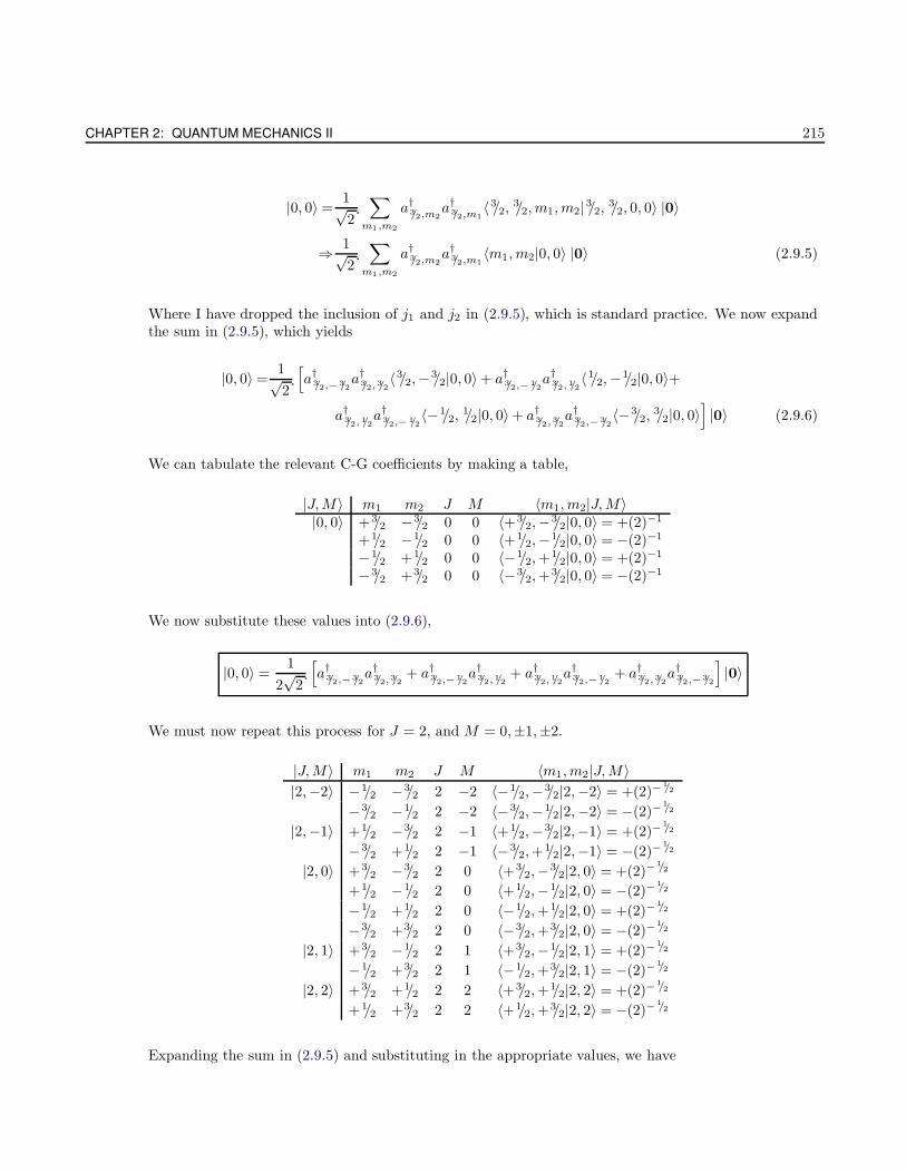
CHAPTER 2: QUANTUM MECHANICS II 215
|0, 0〉 =1√2
∑
m1,m2
a†3/2,m2a†3/2,m1
〈3/2,3/2, m1, m2|3/2, 3/2, 0, 0〉 |0〉
⇒ 1√2
∑
m1,m2
a†3/2,m2a†3/2,m1
〈m1, m2|0, 0〉 |0〉 (2.9.5)
Where I have dropped the inclusion of j1 and j2 in (2.9.5), which is standard practice. We now expandthe sum in (2.9.5), which yields
|0, 0〉 =1√2
[a†3/2,−3/2
a†3/2,3/2〈3/2,−3/2|0, 0〉+ a†3/2,−1/2
a†3/2,1/2〈1/2,−1/2|0, 0〉+
a†3/2,1/2a†3/2,−1/2
〈−1/2,1/2|0, 0〉+ a†3/2,3/2
a†3/2,−3/2〈−3/2,
3/2|0, 0〉]|0〉 (2.9.6)
We can tabulate the relevant C-G coefficients by making a table,
|J,M〉 m1 m2 J M 〈m1, m2|J,M〉|0, 0〉 +3/2 −3/2 0 0 〈+3/2,−3/2|0, 0〉 = +(2)−1
+1/2 −1/2 0 0 〈+1/2,−1/2|0, 0〉 = −(2)−1
−1/2 +1/2 0 0 〈−1/2,+1/2|0, 0〉 = +(2)−1
−3/2 +3/2 0 0 〈−3/2,+3/2|0, 0〉 = −(2)−1
We now substitute these values into (2.9.6),
|0, 0〉 =1
2√
2
[a†3/2,−3/2
a†3/2,3/2+ a†3/2,−1/2
a†3/2,1/2+ a†3/2,1/2
a†3/2,−1/2+ a†3/2,3/2
a†3/2,−3/2
]|0〉
We must now repeat this process for J = 2, and M = 0,±1,±2.
|J,M〉 m1 m2 J M 〈m1, m2|J,M〉|2,−2〉 −1/2 −3/2 2 −2 〈−1/2,−3/2|2,−2〉 = +(2)−
1/2
−3/2 −1/2 2 −2 〈−3/2,−1/2|2,−2〉 = −(2)−1/2
|2,−1〉 +1/2 −3/2 2 −1 〈+1/2,−3/2|2,−1〉 = +(2)−1/2
−3/2 +1/2 2 −1 〈−3/2,+1/2|2,−1〉 = −(2)−
1/2
|2, 0〉 +3/2 −3/2 2 0 〈+3/2,−3/2|2, 0〉 = +(2)−1/2
+1/2 −1/2 2 0 〈+1/2,−1/2|2, 0〉 = −(2)−1/2
−1/2 +1/2 2 0 〈−1/2,+1/2|2, 0〉 = +(2)−
1/2
−3/2 +3/2 2 0 〈−3/2,+3/2|2, 0〉 = −(2)−
1/2
|2, 1〉 +3/2 −1/2 2 1 〈+3/2,−1/2|2, 1〉 = +(2)−1/2
−1/2 +3/2 2 1 〈−1/2,+3/2|2, 1〉 = −(2)−
1/2
|2, 2〉 +3/2 +1/2 2 2 〈+3/2,+1/2|2, 2〉 = +(2)−
1/2
+1/2 +3/2 2 2 〈+1/2,+3/2|2, 2〉 = −(2)−
1/2
Expanding the sum in (2.9.5) and substituting in the appropriate values, we have
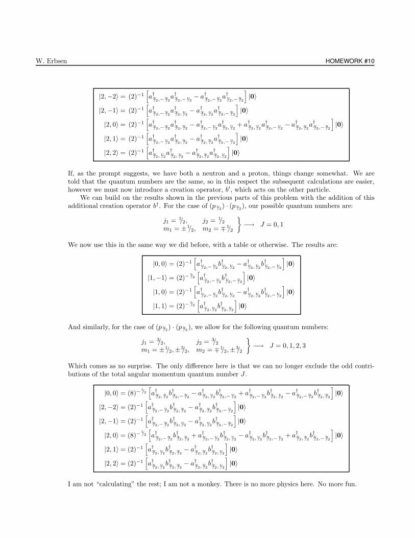
W. Erbsen HOMEWORK #10
|2,−2〉 = (2)−1[a†3/2,−3/2
a†3/2,−1/2− a†3/2,−3/2
a†1/2,−3/2
]|0〉
|2,−1〉 = (2)−1[a†3/2,−3/2
a†3/2,1/2− a†3/2,1/2
a†3/2,−3/2
]|0〉
|2, 0〉 = (2)−1[a†3/2,−3/2
a†3/2,3/2− a†3/2,−1/2
a†3/2,1/2+ a†3/2,1/2
a†3/2,−1/2− a†3/2,3/2
a†3/2,−3/2
]|0〉
|2, 1〉 = (2)−1[a†3/2,−1/2
a†3/2,3/2− a†3/2,3/2
a†3/2,−1/2
]|0〉
|2, 2〉 = (2)−1[a†3/2,1/2
a†3/2,1/2− a†3/2,3/2
a†3/2,1/2
]|0〉
If, as the prompt suggests, we have both a neutron and a proton, things change somewhat. We aretold that the quantum numbers are the same, so in this respect the subsequent calculations are easier,however we must now introduce a creation operator, b′, which acts on the other particle.
We can build on the results shown in the previous parts of this problem with the addition of thisadditional creation operator b†. For the case of (p1/2) · (p1/2), our possible quantum numbers are:
j1 = 1/2, j2 = 1/2m1 = ±1/2, m2 = ∓1/2
−→ J = 0, 1
We now use this in the same way we did before, with a table or otherwise. The results are:
|0, 0〉 = (2)−1[a†1/2,−1/2
b†1/2,1/2− a†1/2,1/2
b†1/2,−1/2
]|0〉
|1,−1〉 = (2)−1/2[a†1/2,−1/2
b†1/2,−1/2
]|0〉
|1, 0〉 = (2)−1[a†1/2,−1/2
b†1/2,1/2− a†1/2,1/2
b†1/2,−1/2
]|0〉
|1, 1〉 = (2)−1/2[a†1/2,1/2
b†1/2,1/2
]|0〉
And similarly, for the case of (p3/2) · (p3/2 ), we allow for the following quantum numbers:
j1 = 3/2, j2 = 3/2m1 = ±1/2,±3/2, m2 = ∓1/2,±3/2
−→ J = 0, 1, 2, 3
Which comes as no surprise. The only difference here is that we can no longer exclude the odd contri-butions of the total angular momentum quantum number J .
|0, 0〉 = (8)−1/2[a†3/2,3/2
b†3/2,−3/2− a†3/2,1/2
b†3/2,−1/2+ a†3/2,−1/2
b†3/2,1/2− a†3/2,−3/2
b†3/2,3/2
]|0〉
|2,−2〉 = (2)−1[a†3/2,−1/2
b†3/2,3/2− a†3/2,3/2
b†3/2,−1/2
]|0〉
|2,−1〉 = (2)−1[a†3/2,−3/2
b†3/2,1/2− a†3/2,1/2
b†3/2,−3/2
]|0〉
|2, 0〉 = (8)−1/2[a†3/2,−3/2
b†3/2,3/2+ a†3/2,−1/2
b†3/2,1/2− a†3/2,1/2
b†3/2,−1/2+ a†3/2,3/2
b†3/2,−3/2
]|0〉
|2, 1〉 = (2)−1[a†3/2,1/2
b†3/2,3/2− a†3/2,3/2
b†3/2,1/2
]|0〉
|2, 2〉 = (2)−1[a†3/2,1/2
b†3/2,3/2− a†3/2,3/2
b†3/2,1/2
]|0〉
I am not “calculating” the rest; I am not a monkey. There is no more physics here. No more fun.
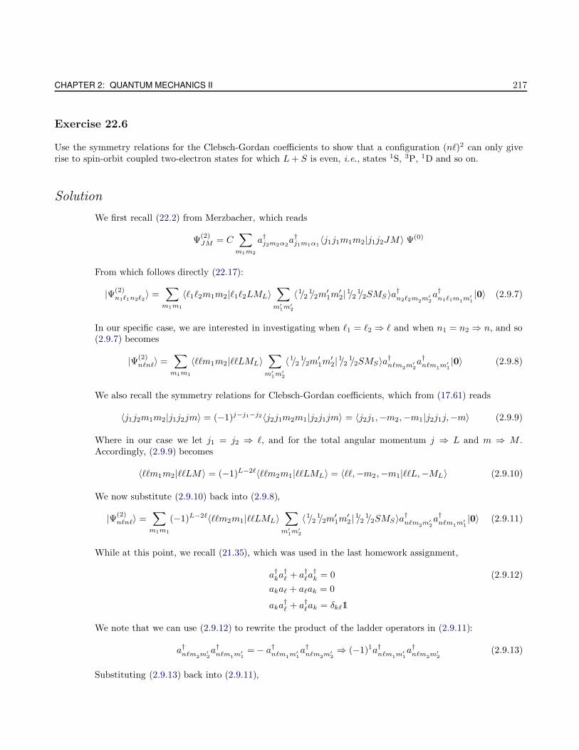
CHAPTER 2: QUANTUM MECHANICS II 217
Exercise 22.6
Use the symmetry relations for the Clebsch-Gordan coefficients to show that a configuration (n`)2 can only giverise to spin-orbit coupled two-electron states for which L+ S is even, i.e., states 1S, 3P, 1D and so on.
Solution
We first recall (22.2) from Merzbacher, which reads
Ψ(2)JM = C
∑
m1m2
a†j2m2α2a†j1m1α1
〈j1j1m1m2|j1j2JM〉 Ψ(0)
From which follows directly (22.17):
|Ψ(2)n1`1n2`2
〉 =∑
m1m1
〈`1`2m1m2|`1`2LML〉∑
m′1m′
2
〈1/21/2m
′1m
′2|1/2 1/2SMS 〉a†n2`2m2m′
2a†n1`1m1m′
1|0〉 (2.9.7)
In our specific case, we are interested in investigating when `1 = `2 ⇒ ` and when n1 = n2 ⇒ n, and so(2.9.7) becomes
|Ψ(2)n`n`〉 =
∑
m1m1
〈``m1m2|``LML〉∑
m′1m′
2
〈1/21/2m
′1m
′2|1/2 1/2SMS〉a†n`m2m′
2a†n`m1m′
1|0〉 (2.9.8)
We also recall the symmetry relations for Clebsch-Gordan coefficients, which from (17.61) reads
〈j1j2m1m2|j1j2jm〉 = (−1)j−j1−j2〈j2j1m2m1|j2j1jm〉 = 〈j2j1,−m2,−m1|j2j1j,−m〉 (2.9.9)
Where in our case we let j1 = j2 ⇒ `, and for the total angular momentum j ⇒ L and m ⇒ M .Accordingly, (2.9.9) becomes
〈``m1m2|``LM〉 = (−1)L−2`〈``m2m1|``LML〉 = 〈``,−m2 ,−m1|``L,−ML〉 (2.9.10)
We now substitute (2.9.10) back into (2.9.8),
|Ψ(2)n`n`〉 =
∑
m1m1
(−1)L−2`〈``m2m1|``LML〉∑
m′1m′
2
〈1/21/2m
′1m
′2 |1/2 1/2SMS〉a†n`m2m′
2a†n`m1m′
1|0〉 (2.9.11)
While at this point, we recall (21.35), which was used in the last homework assignment,
a†ka†` + a†`a
†k = 0 (2.9.12)
aka` + a`ak = 0
aka†` + a†`ak = δk`1
We note that we can use (2.9.12) to rewrite the product of the ladder operators in (2.9.11):
a†n`m2m′2a†n`m1m′
1= − a†n`m1m′
1a†n`m2m′
2⇒ (−1)1a†n`m1m′
1a†n`m2m′
2(2.9.13)
Substituting (2.9.13) back into (2.9.11),
W. Erbsen HOMEWORK #10
|Ψ(2)n`n`〉 =
∑
m1m1
(−1)L−2`+1〈``m2m1|``LML〉∑
m′1m′
2
〈1/21/2m
′1m
′2|1/2 1/2SMS〉a†n`m1m′
1a†n`m2m′
2|0〉 (2.9.14)
⇒(−1)L+S−2`|Ψ(2)n`n`〉 (2.9.15)
The required condition is satisfied, i.e. unless L+ S is even, (2.9.14) is violated .
Exercise 22.10
Show that the configuration space wave function corresponding to the independent particle state (22.22) canbe expressed as the Slater determinant
ψ(r1σ1, · · · , rNσN) =1√N !
∣∣∣∣∣∣∣∣∣
ψ1(r1σ1) ψ1(r2σ2) · · · ψ1(rNσN)ψ2(r1σ1) ψ2(r2σ2) · · · ψ2(rNσN)
......
. . ....
ψn(r1σ1) ψn(r2σ2) · · · ψn(rNσN)
∣∣∣∣∣∣∣∣∣(2.9.16)
Solution
We first recall that (22.22) from Merzbacher reads
|Ψν〉 = a†Na†N−1 · · ·a
†2a
†1 |0〉 (2.9.17)
While we must always obey the symmetrixation requirement :
ψ(r1, r2) = ±ψ(r2, r1)
Treating this in a more explicit manner,
ψ±(r1, r2) =1√2
[ψa(r1)ψb(r2) ± ψb(r1)ψa(r2)] (2.9.18)
Where the upper sign represents Bosons, while the lower is for Fermions. Directly from (2.9.18) followsthe Pauli Exclusion Principle, which applies only to Fermions. For two particles that occupy the samestate ψa = ψb,
ψ−(r1, r2) =1√2
[ψa(r1)ψa(r2) − ψa(r2)ψa(r1)] ⇒ 0
In other words, the resultant wave function must be anti-symmetric with the exchange of any twoparticles. We note that while the previous equations do not contain an explicit spin dependence, onemay be included without loss of generality. Accordingly, (2.9.18) becomes
ψ±(r1σ1, r2σ2) =1√2
[ψa(r1σ1)ψb(r2σ2) ± ψa(r2σ2)ψb(r1σ1)] (2.9.19)
CHAPTER 2: QUANTUM MECHANICS II 219
In this special two-particle case, it is not hard to see that we can rewrite (2.9.19) in terms of a determinant:
ψ±(r1σ1, r2σ2) =1√2
∣∣∣∣ψa(r1σ1) ψa(r2σ2)ψb(r1σ1) ψb(r2σ2)
∣∣∣∣ (2.9.20)
The extension of (2.9.19) to (2.9.20) may be generalized to a N -particle system without too much trouble;all we have to do is recognize that the odd exchanges in the wave function product terms must includea factor of −1. Explicitly, we rewrite (2.9.20) for N particles as:
ψ±(r1σ1, r2σ2, · · · , rNσN) =1√2
[ψa(r1σ1)ψb(r2σ2) · · ·ψN (rNσN ) ± ψa(r2σ2)ψb(r1σ1) · · ·ψN (rNσN)]
(2.9.21)
Where we note that the complete set of wave function denominations is ψa, ψb, ..., ψN . We canimmediately rewrite (2.9.21) in the form of a determinant, as suggested by the prompt:
ψ(r1σ1, · · · , rNσN ) =1√N !
∣∣∣∣∣∣∣∣∣
ψa(r1σ1) ψa(r2σ2) · · · ψa(rNσN )ψb(r1σ1) ψb(r2σ2) · · · ψb(rNσN)
......
. . ....
ψN (r1σ1) ψN (r2σ2) · · · ψN (rNσN )
∣∣∣∣∣∣∣∣∣
Which is the same as (2.9.16).
Problem 22.6
Apply the Hartree-Fock method to a system of two “electrons” which are attracted to the coordinate originby an isotropic harmonic oscillator potential mω2r2/2 and which interact with each other through a potentialV = C(r′ − r′′)2. Solve the Hartree-Fock equations for the ground state and compare with the exact result andwith first-order perturbation theory.
Solution
Due to the phrasing of the problem, we are inclined to utilize the symmetry around the origin. We alsoknow that the Hamiltonian for this system is just the sum of the Harmonic oscillator Hamiltonian plusthe interaction term:
H = − ~2
2m∇
2 +mω2
2r2 − V (2.9.22)
Applying V from the prompt to (2.9.22),∗
H = − ~2
2m
(∇
21 + ∇
22
)+mω2
2
(r21 + r2
2
)− C(r1 − r2)
2 (2.9.23)
∗I have replace Merzbacher’s silly prime notation with my selected subscripts to deter ambiguity between various notations.
W. Erbsen HOMEWORK #10
At this point, we seemingly arbitrarily, introduce the relative and center of mass coordinate variablesrespectively:
r =1√2
(r1 − r2) , R =1√2
(r1 + r2) (2.9.24)
Rewriting (2.9.23) according to (2.9.24),
H = − ~2
2m
(∇
21 + ∇
22
)+mω2
2R2 − Cr2 (2.9.25)
If we introduce the following similar coordinates for the momenta,
p =1√2
(p1 − p2) , P =1√2
(p1 + p2) (2.9.26)
Rewriting the kinetic energy term from (2.9.25) in terms momentum variables and utilizing (2.9.26), wehave∗
H =1
2
(P2 + R2
)+
1
2
[p2 + r2
√2C + 1
](2.9.27)
From this, we can see that by the use of our chosen transformations from (2.9.24) and (2.9.26), we seethat we have turned one Hamiltonian into two independent 3-dimensional harmonic oscillators.
This problem has been presented before; the (exact) results are
Ψ(r,R) =
(2C + 1
π4
) 3/8
exp
[−R2
2
]exp
[−√
2C + 1
2r2
](2.9.28a)
E0 =3
2
[1 +
√2C + 1
](2.9.28b)
To see how the Hartree-Fock (HF) perspective compares to (2.9.28a) and (2.9.28b), we see that
ΨHF =1√2
∣∣∣∣ψ(r1)χ+ ψ(r2)χ+
ψ(r1)χ− ψ(r2)χ−
∣∣∣∣ (2.9.29)
And the HF equation for our Hamiltonian becomes
1
2
[p2
1 + r21
]ψ(r1) +
1
2
[∫ψ∗(r2) · C (r1 − r2)
2 · ψ(r2) dr2
]ψ(r1) = Eψ(r1) (2.9.30)
If we expand the central term in (2.9.30), we find that
(r1 − r2)2
= r21 + r2
2 − 2r1 · r2 (2.9.31)
The last term in (2.9.31) vanishes in the integral due to parity. Therefore, the integral becomes trivialand (2.9.30) yields
Ψ0(r1) =
(C + 1
π2
) 3/8
exp
[−√C + 1
2r21
]
∗Atomic units and also ω = 1.
CHAPTER 2: QUANTUM MECHANICS II 221
E0 =3
2
(3C + 2
2C + 2
)√C + 1
And so the Hartree-Fock ground state wave function becomes
ΨHF0 (r,R) =
(C + 1
π4
)3/8
exp
[−√C + 1
2
(r2 + R2
)](2.9.33)
And now, the energy eigenvalues according to (2.9.33) can be found by taking the expectation value ofour Hamiltonian from (2.9.25) with the HF state from (2.9.33). The result is ?
EHF0 = 〈ΨHF
0 |H|ΨHF0 〉 −→ EHF
0 = 3√C + 1 (2.9.34)
Please see attached Mathematica printout with plots.
W. Erbsen *
Appendix A *
Creation and Annihilation Operators
We first recall from class that the action of the creation and annihilation operators on an arbitrary vector |ψn〉acts like:
a†|ψn〉 =√n+ 1 |ψn+1〉 (A.1a)
a|ψn〉 =√n |ψn−1〉 (A.1b)
We also recall that the position and momentum operators are given in terms of the creation and annihilationoperators as:
x =
√~
2mω
(a† + a
)(A.2a)
p =
√~mω
2
(a† − a
)(A.2b)
We can now find the expectation values of various combinations of ladder operators, namely 〈a†〉, 〈a〉, 〈a†a〉, 〈aa†〉,〈a2〉, and 〈a†2〉:
〈a†〉 =〈ψn′(x)|a†|ψn(x)〉
=
∫ ∞
−∞ψ∗
n′(x)a†ψn(x) dx
=
∫ ∞
−∞ψ∗
n′(x)(√n+ 1 ψn+1(x)
)dx
=√n + 1 δn′,n+1 (A.3)
〈a〉 =〈ψn′(x)|a|ψn(x)〉
=
∫ ∞
−∞ψ∗
n′(x)aψn(x) dx
=
∫ ∞
−∞ψ∗
n′(x)(√n ψn−1(x)
)dx
=√n δn′,n−1 (A.4)
〈a†a〉 =〈ψn′(x)|a†a|ψn(x)〉
=
∫ ∞
−∞ψ∗
n′(x)a†aψn(x) dx
=
∫ ∞
−∞ψ∗
n′(x)a†(√n ψn−1(x)
)dx
=
∫ ∞
−∞ψ∗
n′(x) (nψn(x)) dx
=nδn′,n (A.5)
〈aa†〉 =〈ψn′(x)|aa†|ψn(x)〉
CHAPTER 2: QUANTUM MECHANICS II 223
=
∫ ∞
−∞ψ∗
n′(x)aa†ψn(x) dx
=
∫ ∞
−∞ψ∗
n′(x)a(√n+ 1 ψn+1(x)
)dx
=
∫ ∞
−∞ψ∗
n′(x) ((n+ 1)ψn(x)) dx
=(n+ 1)δn′,n (A.6)
〈a†2〉 =〈ψn′(x)|a†2|ψn(x)〉
=
∫ ∞
−∞ψ∗
n′(x)a†a†ψn(x) dx
=
∫ ∞
−∞ψ∗
n′(x)a†(√n+ 1 ψn+1(x)
)dx
=
∫ ∞
−∞ψ∗
n′(x) ((n+ 1)ψn+2(x)) dx
=(n+ 1)δn′,n+2 (A.7)
〈a2〉 =〈ψn′(x)|a2|ψn(x)〉
=
∫ ∞
−∞ψ∗
n′(x)aaψn(x) dx
=
∫ ∞
−∞ψ∗
n′(x)a(√n ψn−1(x)
)dx
=
∫ ∞
−∞ψ∗
n′(x) (nψn−2(x)) dx
=nδn′,n−2 (A.8)
We now wish to find the expectation values of the position and momentum operators from (A.2a) and (A.2b), andalso their square. We can do this by using (A.3)-(A.8):
〈x〉 =
√~
2mω〈(a† + a)〉
=
√~
2mω
(〈a†〉 + 〈a〉
)
=
√~
2mω
(√n+ 1 δn′,n+1 +
√n δn′,n−1
)
=0 (A.9)
〈x2〉 =~
2mω〈(a† + a)2〉
=~
2mω〈(a†2 + a†a + aa† + a2)〉
=~
2mω
(〈a†2〉 + 〈a†a〉 + 〈aa†〉 + 〈a2〉
)
W. Erbsen *
=~
2mω((n + 1)δn′,n+2 + nδn′,n + (n+ 1)δn′,n + nδn′,n−2)
=~
2mω(n(n + 1))
=~
2mω(2n+ 1) (A.10)
〈p〉 =i
√~mω
2〈(a† + a)〉
=i
√~mω
2
(〈a†〉 + 〈a〉
)
=i
√~mω
2
(√n+ 1 δn′,n+1 +
√n δn′,n−1
)
=0 (A.11)
〈p2〉 = − ~mω
2〈(a† − a)2〉
= − ~mω
2〈(a†2 − a†a− aa† + a2)〉
= − ~mω
2
(〈a†2〉 − 〈a†a〉 − 〈aa†〉 + 〈a2〉
)
= − ~mω
2((n+ 1)δn′,n+2 − nδn′,n − (n + 1)δn′,n + nδn′,n−2)
= − ~mω
2(−n− (n+ 1))
=~mω
2(2n+ 1) (A.12)
CHAPTER 2: QUANTUM MECHANICS II 225
Appendix B *
Hermite Polynomial Recursion RelationEquation (5.35) from Merzbacher reads:
Hn(ξ) =
(dn
dsneξ2−(s−ξ)2
)
s=0
=(−1)neξ2 dn
dξne−ξ2
(B.1)
Which is known as Rodrigues’ formula for Hermite Polynomials. To derive the recursion relation, we first differ-entiate Hn(ξ):
d
dξHn(ξ) =
d
dξ
((−1)neξ2
(d
dξ
)n
e−ξ2
)
=(−1)n
(d
dξeξ2
)(d
dξ
)n
+ (−1)neξ2
(d
dξ
)n+1
e−ξ2
=2x(−1)neξ2
(d
dξ
)n
− (−1)n+1eξ2
(d
dξ
)n+1
e−ξ2
=2xHn(ξ) −Hn+1(ξ) (B.2)
And from Eq. (5.32) in Merzbacher we know that
d
dξHnξ = 2nHn−1(ξ)
So that (B.2) becomes:
2nHn−1(ξ) = 2xHn(ξ) −Hn+1(ξ) (B.3)
And from (B.3) we finally arrive at the recursion relation,
Hn+1(ξ) = 2xHn(ξ) − 2nHn−1(ξ) (B.4)
Which agrees with Abramowitz and Stegun, pg. 782 22.7.13 ?.

W. Erbsen *
clearemptydoublepage
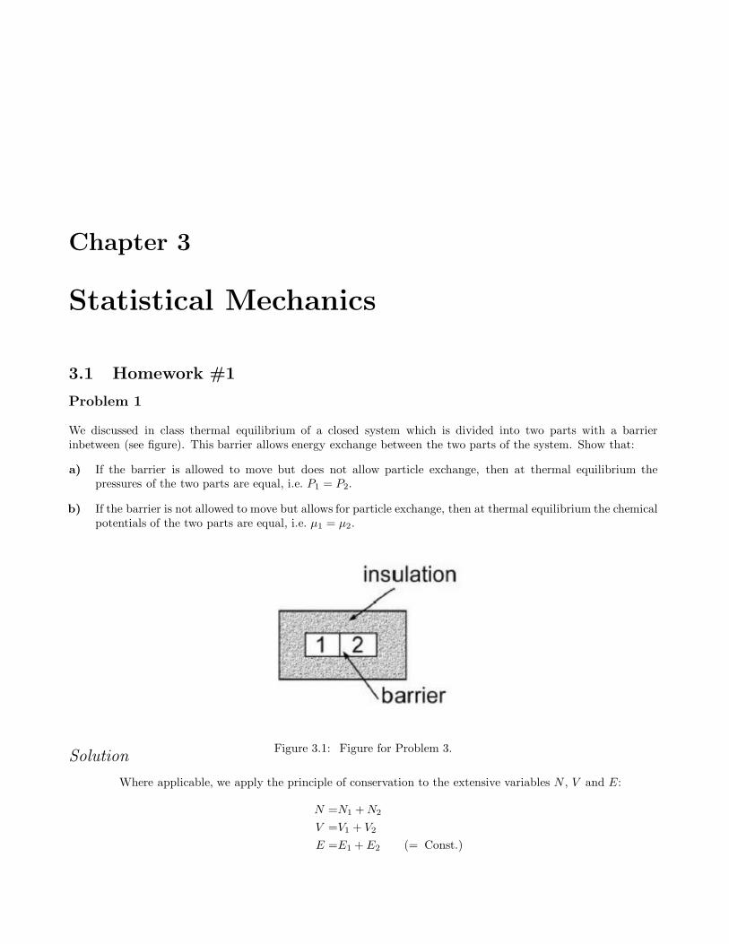
Chapter 3
Statistical Mechanics
3.1 Homework #1
Problem 1
We discussed in class thermal equilibrium of a closed system which is divided into two parts with a barrierinbetween (see figure). This barrier allows energy exchange between the two parts of the system. Show that:
a) If the barrier is allowed to move but does not allow particle exchange, then at thermal equilibrium thepressures of the two parts are equal, i.e. P1 = P2.
b) If the barrier is not allowed to move but allows for particle exchange, then at thermal equilibrium the chemicalpotentials of the two parts are equal, i.e. µ1 = µ2.
Figure 3.1: Figure for Problem 3.Solution
Where applicable, we apply the principle of conservation to the extensive variables N , V and E:
N =N1 +N2
V =V1 + V2
E =E1 + E2 (= Const.)
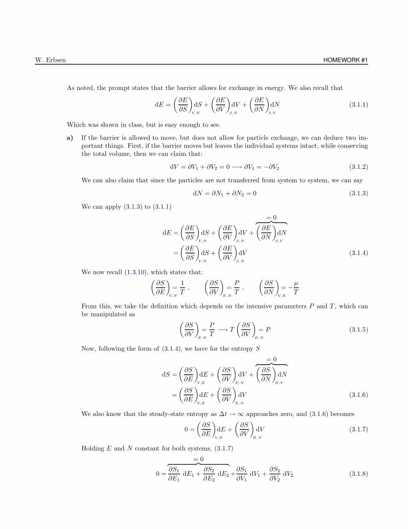
W. Erbsen HOMEWORK #1
As noted, the prompt states that the barrier allows for exchange in energy. We also recall that
dE =
(∂E
∂S
)
V,N
dS +
(∂E
∂V
)
S,N
dV +
(∂E
∂N
)
S,V
dN (3.1.1)
Which was shown in class, but is easy enough to see.
a) If the barrier is allowed to move, but does not allow for particle exchange, we can deduce two im-portant things. First, if the barrier moves but leaves the individual systems intact, while conservingthe total volume, then we can claim that:
dV = ∂V1 + ∂V2 = 0 −→ ∂V1 = −∂V2 (3.1.2)
We can also claim that since the particles are not transferred from system to system, we can say
dN = ∂N1 + ∂N2 = 0 (3.1.3)
We can apply (3.1.3) to (3.1.1)
dE =
(∂E
∂S
)
V,N
dS +
(∂E
∂V
)
S,N
dV +
= 0︷ ︸︸ ︷(∂E
∂N
)
S,V
dN
=
(∂E
∂S
)
V,N
dS +
(∂E
∂V
)
S,N
dV (3.1.4)
We now recall (1.3.10), which states that:(∂S
∂E
)
V,N
=1
T,
(∂S
∂V
)
E,N
=P
T,
(∂S
∂N
)
V,E
= −µ
T
From this, we take the definition which depends on the intensive parameters P and T , which canbe manipulated as
(∂S
∂V
)
E,N
=P
T−→ T
(∂S
∂V
)
E,N
= P (3.1.5)
Now, following the form of (3.1.4), we have for the entropy S
dS =
(∂S
∂E
)
V,E
dE +
(∂S
∂V
)
E,N
dV +
= 0︷ ︸︸ ︷(∂S
∂N
)
E,V
dN
=
(∂S
∂E
)
V,E
dE +
(∂S
∂V
)
E,N
dV (3.1.6)
We also know that the steady-state entropy as ∆t → ∞ approaches zero, and (3.1.6) becomes
0 =
(∂S
∂E
)
V,E
dE +
(∂S
∂V
)
E,N
dV (3.1.7)
Holding E and N constant for both systems, (3.1.7)
0 =
= 0︷ ︸︸ ︷∂S1
∂E1dE1 +
∂S2
∂E2dE2 +
∂S1
∂V1dV1 +
∂S2
∂V2dV2 (3.1.8)
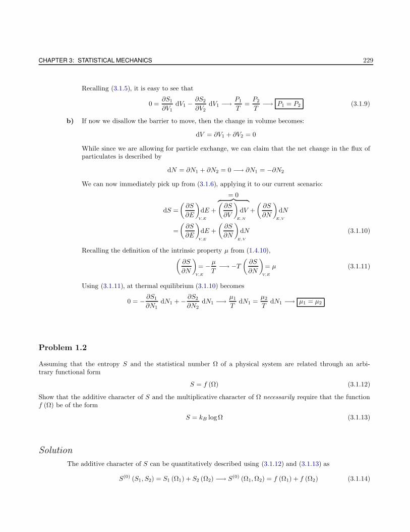
CHAPTER 3: STATISTICAL MECHANICS 229
Recalling (3.1.5), it is easy to see that
0 =∂S1
∂V1dV1 −
∂S2
∂V2dV1 −→ P1
T=P2
T−→ P1 = P2 (3.1.9)
b) If now we disallow the barrier to move, then the change in volume becomes:
dV = ∂V1 + ∂V2 = 0
While since we are allowing for particle exchange, we can claim that the net change in the flux ofparticulates is described by
dN = ∂N1 + ∂N2 = 0 −→ ∂N1 = −∂N2
We can now immediately pick up from (3.1.6), applying it to our current scenario:
dS =
(∂S
∂E
)
V,E
dE +
= 0︷ ︸︸ ︷(∂S
∂V
)
E,N
dV +
(∂S
∂N
)
E,V
dN
=
(∂S
∂E
)
V,E
dE +
(∂S
∂N
)
E,V
dN (3.1.10)
Recalling the definition of the intrinsic property µ from (1.4.10),(∂S
∂N
)
V,E
= − µ
T−→ −T
(∂S
∂N
)
V,E
= µ (3.1.11)
Using (3.1.11), at thermal equilibrium (3.1.10) becomes
0 = − ∂S1
∂N1dN1 + − ∂S2
∂N2dN1 −→ µ1
TdN1 =
µ2
TdN1 −→ µ1 = µ2
Problem 1.2
Assuming that the entropy S and the statistical number Ω of a physical system are related through an arbi-trary functional form
S = f (Ω) (3.1.12)
Show that the additive character of S and the multiplicative character of Ω necessarily require that the functionf (Ω) be of the form
S = kB logΩ (3.1.13)
Solution
The additive character of S can be quantitatively described using (3.1.12) and (3.1.13) as
S(0) (S1, S2) = S1 (Ω1) + S2 (Ω2) −→ S(0) (Ω1,Ω2) = f (Ω1) + f (Ω2) (3.1.14)
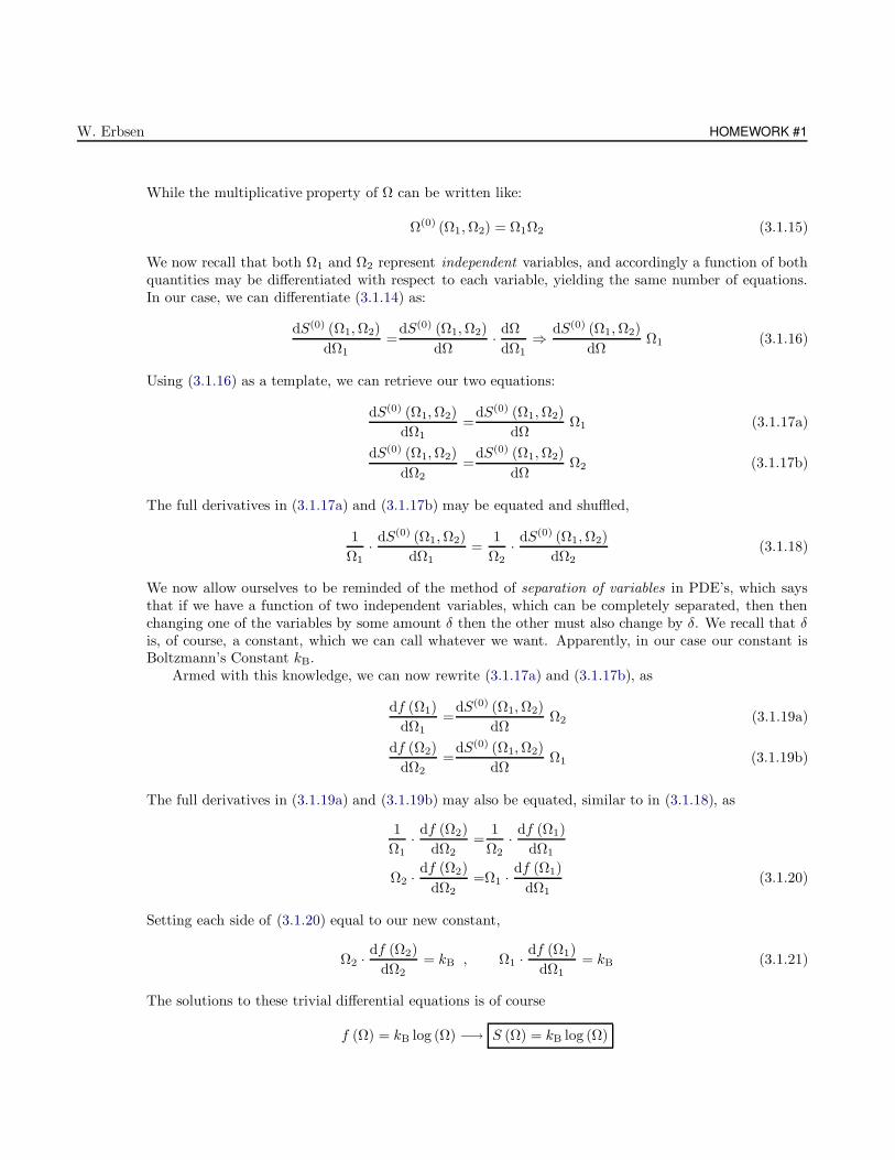
W. Erbsen HOMEWORK #1
While the multiplicative property of Ω can be written like:
Ω(0) (Ω1,Ω2) = Ω1Ω2 (3.1.15)
We now recall that both Ω1 and Ω2 represent independent variables, and accordingly a function of bothquantities may be differentiated with respect to each variable, yielding the same number of equations.In our case, we can differentiate (3.1.14) as:
dS(0) (Ω1,Ω2)
dΩ1=
dS(0) (Ω1,Ω2)
dΩ· dΩ
dΩ1⇒ dS(0) (Ω1,Ω2)
dΩΩ1 (3.1.16)
Using (3.1.16) as a template, we can retrieve our two equations:
dS(0) (Ω1,Ω2)
dΩ1=
dS(0) (Ω1,Ω2)
dΩΩ1 (3.1.17a)
dS(0) (Ω1,Ω2)
dΩ2=
dS(0) (Ω1,Ω2)
dΩΩ2 (3.1.17b)
The full derivatives in (3.1.17a) and (3.1.17b) may be equated and shuffled,
1
Ω1· dS(0) (Ω1,Ω2)
dΩ1=
1
Ω2· dS(0) (Ω1,Ω2)
dΩ2(3.1.18)
We now allow ourselves to be reminded of the method of separation of variables in PDE’s, which saysthat if we have a function of two independent variables, which can be completely separated, then thenchanging one of the variables by some amount δ then the other must also change by δ. We recall that δis, of course, a constant, which we can call whatever we want. Apparently, in our case our constant isBoltzmann’s Constant kB.
Armed with this knowledge, we can now rewrite (3.1.17a) and (3.1.17b), as
df (Ω1)
dΩ1=
dS(0) (Ω1,Ω2)
dΩΩ2 (3.1.19a)
df (Ω2)
dΩ2=
dS(0) (Ω1,Ω2)
dΩΩ1 (3.1.19b)
The full derivatives in (3.1.19a) and (3.1.19b) may also be equated, similar to in (3.1.18), as
1
Ω1· df (Ω2)
dΩ2=
1
Ω2· df (Ω1)
dΩ1
Ω2 ·df (Ω2)
dΩ2=Ω1 ·
df (Ω1)
dΩ1(3.1.20)
Setting each side of (3.1.20) equal to our new constant,
Ω2 ·df (Ω2)
dΩ2= kB , Ω1 ·
df (Ω1)
dΩ1= kB (3.1.21)
The solutions to these trivial differential equations is of course
f (Ω) = kB log (Ω) −→ S (Ω) = kB log (Ω)
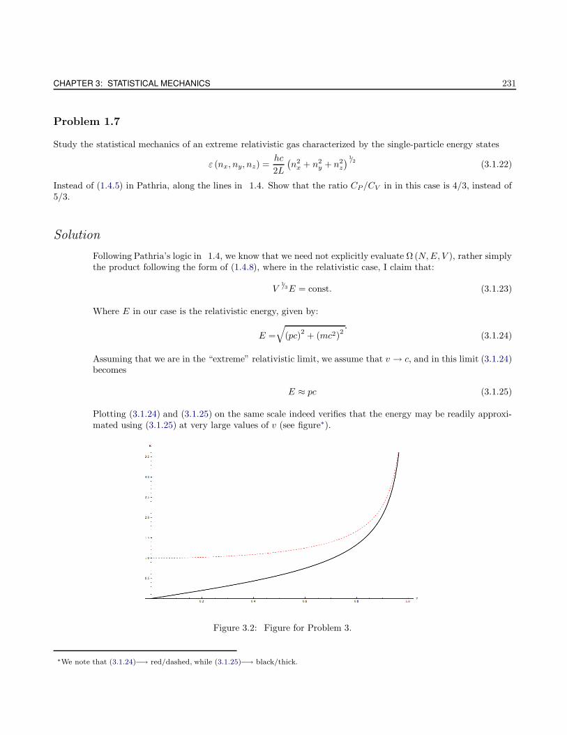
CHAPTER 3: STATISTICAL MECHANICS 231
Problem 1.7
Study the statistical mechanics of an extreme relativistic gas characterized by the single-particle energy states
ε (nx, ny, nz) =hc
2L
(n2
x + n2y + n2
z
)1/2(3.1.22)
Instead of (1.4.5) in Pathria, along the lines in 1.4. Show that the ratio CP/CV in in this case is 4/3, instead of5/3.
Solution
Following Pathria’s logic in 1.4, we know that we need not explicitly evaluate Ω (N,E, V ), rather simplythe product following the form of (1.4.8), where in the relativistic case, I claim that:
V1/3E = const. (3.1.23)
Where E in our case is the relativistic energy, given by:
E =
√(pc)
2+ (mc2)
2(3.1.24)
Assuming that we are in the “extreme” relativistic limit, we assume that v → c, and in this limit (3.1.24)becomes
E ≈ pc (3.1.25)
Plotting (3.1.24) and (3.1.25) on the same scale indeed verifies that the energy may be readily approxi-mated using (3.1.25) at very large values of v (see figure∗).
Figure 3.2: Figure for Problem 3.
∗We note that (3.1.24)−→ red/dashed, while (3.1.25)−→ black/thick.
W. Erbsen HOMEWORK #1
Furthermore, we can build on (1.4.6) by noting that the expression for Ω (N,E, V ) depends on thenumber of independent, positive-integral solutions as prescribed by:
2L
hcε =
(n2
x + n2y + n2
z
)1/2(3.1.26)
From the Maxwell-Boltzmann Distribution Function, and (3.1.25). Furthermore, we recall that V = L3,and so (3.1.26) becomes
2
hcV
1/3ε (nx, ny, nz) =(n2
x + n2y + n2
z
) 1/2 −→ ε (nx, ny, nz) =hc
2L
(n2
x + n2y + n2
z
)1/2(3.1.27)
Where we can see from (3.1.27) where (3.1.23) was derived from. Furthermore, using (1.4.25), we cansay that:
P = −(∂E
∂V
)
N,S
= − ∂
∂V
[Const. · V −1/3
]
=Const. · 1
3· V −4/3
=Const. · V −4/3 (3.1.28)
It is easy to see from (3.1.28) that our condition for a reversible adiabatic process is given by
PV4/3 = Const. (3.1.29)
Where the raised power of V in (3.1.29) is none other than γ, so we can finally say:
γ =CP
CV−→ γ =
4
3
Problem 1.13
If the two gases considered in the mixing process of 1.5 were initially at different temperatures, say T1 andT2, what would the entropy of mixing be in that case? Would the contribution arising from this cause depend onwhether the two gases were different or identical?
Solution
We first recall from (1.5.13) that
Si = NikB log [Vi] +3
2NikB
1 + log
[2πmikBT
h2
]; i = 1, 2 (3.1.30)
Which represents the entropy before the mixing ever took place. If we allow our systems to start atdifferent temperatures, (3.1.30) becomes
CHAPTER 3: STATISTICAL MECHANICS 233
Si = NikB log [Vi] +3
2NikB
1 + log
[2πmikBTi
h2
]; i = 1, 2 (3.1.31)
Where it should be mentioned that the only thing changed is the addition of an index to the intensivevariable T . Regrouping and realigning (3.1.31), we have
Si =3
2kBNi
2
3log [Vi] + log [αmiTi] + 1
(3.1.32)
Where I have assigned the constant α to be defined by
α =2πkB
h2(3.1.33)
Following the convention of (3.1.32), we can say that the post-mixing entropy is (analogous to (1.5.2)):
ST =3
2kB
2∑
i=1
Ni
2
3log [V ] + log [αmiT ] + 1
(3.1.34)
The increase in ∆S, called the entropy of mixing, is then given by
∆S = ST −2∑
i=1
Si (3.1.35)
The first term in (3.1.35) is found from (3.1.34) to be
ST =3
2kB
[N1
2
3log [V ] + log [αm1T ] + 1
+N2
2
3log [V ] + log [αm2T ] + 1
](3.1.36)
While the sum in (3.1.35) is found from (3.1.32) to be
2∑
i=1
=3
2kB
[N1
2
3log [V1] + log [αm1T1] + 1
+N2
2
3log [V2] + log [αm2T2] + 1
](3.1.37)
Before we take the difference of (3.1.36) and (3.1.37), thus completing the saga of (3.1.35), we note thatthis page width is finite (countable, har har), we drop the terms which obviously cancel. I will alsoconsolidate a few things. Continuing,
∆S =3
2kB
[N1
2
3log
[V
V1
]+ log
[T
T1
]+N2
2
3log
[V
V2
]+ log
[T
T2
]](3.1.38)
Jostling things about a bit, (3.1.38) becomes
∆S = kBN1
log
[V1 + V2
V1
]+ log
[T
T1
]3/2
+ kBN2
log
[V1 + V2
V2
]+ log
[T
T2
]3/2
(3.1.39)
The contribution of entropy in (3.1.39) most certainly depends on whether the gases are distinguishableor indistinguishable. This is the setup for Gibbs Paradox. The general idea is that if the particles inboth systems are distinguishable, then after equilibrium is reached, the gas particles may be separatedback into their original compartments, assuming that we can reinsert the partition quickly enough. This
W. Erbsen HOMEWORK #1
would correspond to a reversible process, where we know that the change in entropy, or the entropy ofmixing, must be zero.
If the particles are indistinguishable, then there is no hope of separating them, and so we have anirreversible process, and the entropy must increase.
Problem 1.16
Establish thermodynamically the formulae
V
(∂P
∂T
)
µ
=S (3.1.40a)
V
(∂P
∂µ
)
T
=N (3.1.40b)
Express the pressure P of an ideal classical gas in terms of the variables µ and T , and verify the above formulae.
Solution
We first recall that within the framework of the Grand Canonical Ensemble, where particle exchange isallowed, we can define the following thermodynamic potential:
Ω = F − µdN −→ dΩ = −SdT −Ndµ− PdV (3.1.41)
Where we must recognize that this new thermodynamic potential is not the same as the multiplicity.For our case, (3.1.40a) becomes
dΩ = −SdT︸︷︷︸= 0
−Ndµ︸ ︷︷ ︸= 0
−PdV −→ Ω = −PdV (3.1.42)
Where, following the example of other thermodynamic potentials, we may deduce that
S = −(∂Ω
∂T
)
µ
(3.1.43a)
N = −(∂Ω
∂µ
)
T
(3.1.43b)
Substituting (3.1.42) into (3.1.43a) and (3.1.43b) yields
S = −(∂ (−PV )
∂T
)
µ
−→ S = V
(∂P
∂T
)
µ
(3.1.44a)
N = −(∂ (−PV )
∂µ
)
T
−→ N = V
(∂P
∂µ
)
T
(3.1.44b)
Where we can see that (3.1.44a) is the same as (3.1.40a), while (3.1.44b) is identical to (3.1.40b).
CHAPTER 3: STATISTICAL MECHANICS 235
We now recall that the Gibbs Sum, which is sort of like the partition function for the Grand CanonicalEnsemble, is given by
Ω (µ, T ) =
∞∑
N=0
∑
s(N)
exp
[Nµ− Es,N
kBT
](3.1.45)
While the pressure is
P =kBT
Vlog [Ω (µ, T )] (3.1.46)
Substituting (3.1.45) into (3.1.46), and then plugging the results in to (3.1.40a) and (3.1.40b) in turncauses the terms to collapse, which is readily seen qualitatively.
3.2 Homework #2
Problem 1
In this problem, you will find an expression for entropy in terms of the canonical distribution function ρs = e−βEs
Z
where the partition function Z is given by Z =∑
s e−Es/kBT .
Solution
We first recall that the entropy is defined in terms of the free energy as:
S = −(∂F
∂T
)
V,N
(3.2.1)
While the free energy is given by
F = −kBT log [Z] (3.2.2)
Substituting (3.2.2) into (3.2.1), we have:
S =∂
∂TkBT log [Z] (3.2.3)
And since Z of course depends on T , we carry the partial derivative out as:
S =kB log [Z] + kBT
∂
∂Tlog [Z]
=kB log [Z] + kBT1
Z
∂Z
∂T
(3.2.4)
The bracketed term in (3.2.4) becomes:
W. Erbsen HOMEWORK #2
∂Z
∂T=∂
∂T
∑
s
exp
[− Es
kBT
]
=1
kBT 2
∑
s
Es exp
[− Es
kBT
](3.2.5)
Substituting (3.2.5) back into (3.2.4) yields
S =kB log [Z] + kBT1
Z
1
kBT 2
∑
s
Es exp
[− Es
kBT
]
=kB
(log [Z] +
1
kBT
∑
s
Es1
Zexp
[− Es
kBT
]
︸ ︷︷ ︸ρs
)
=kB
(log [Z] +
1
kBT
∑
s
Esρs
)
= − kB
(− log [Z] +
∑
s
ρs
(− Es
kBT
))
= − kB
(− log [Z] +
∑
s
ρs log
[exp
[− Es
kBT
]])
= − kB
(∑
s
ρs log
[1
Zexp
[− Es
kBT
]
︸ ︷︷ ︸ρs
])(3.2.6)
At this point, we can trivially rewrite (3.2.6) as:
S = −kB
(∑
s
ρs log [ρs]
)
Problem 2
The expression S = −kB
∑r Pr logPr is accepted as the general definition of the entropy of a system. Now
imagine that a system A1 has probability P(1)r of being found in a state r and a system A2 has probability P
(2)s of
being found in a state s. Then one has
S1 = − kB
∑
r
P (1)r logP (1)
r
S2 = − kB
∑
s
P (2)s logP (2)
s
Each state of the composite system A consisting of A1 and A2 can then be labeled by the pair of numbers r, s.Let the probability of A being found in this state be denoted by Prs. Then its entropy is defined as
S = −kB
∑
r
∑
s
Prs logPrs (3.2.7)
CHAPTER 3: STATISTICAL MECHANICS 237
All the probabilities are normalized so that∑
r
P (1)r =1
∑
s
P (2)s =1
∑
r
∑
s
Prs =1
a) If A1 and A2 are weakly interacting so that they are statistically independent, then Prs = P(1)r P
(2)s . Show
that under these circumstances the entropy is additive, i.e. S = S1 + S2.
b) If A1 and A2 are not weakly interacting Prs 6= P(1)r P
(2)s , but the general solutions still hold:
P (1)r =
∑
s
Prs
P (2)s =
∑
r
Prs
Show that
S − (S1 + S2) = kB
∑
r,s
Prs log
(P
(1)r P
(2)s
Prs
)(3.2.8)
and use the inequality log x ≤ (x− 1) to show that S ≤ (S1 + S2). This means that the existence ofcorrelations between the systems, due to the interactions between them, leads to a situation less random thanthat where the systems are completely independent of each other.
Solution
a) Applying our assumption to (3.2.7), we have:
S = − kB
∑
r
∑
s
PrPs log [PrPs]
= − kB
∑
r
∑
s
PrPs log [Pr] + log [Ps]
= − kB
∑
r
∑
s
PrPs log [Pr] + PrPs log [Ps]
= − kB
∑
r
∑
s
PrPs log [Pr] +∑
r
∑
s
PrPs log [Ps]
= − kB
∑
s
Ps
∑
r
Pr log [Pr] +∑
r
Pr
∑
s
Ps log [Ps]
(3.2.9)
We recall from the previous problem that S = −kB
∑i ρi log [ρi], and applying this to (3.2.9) leads
us to:
S = − kB
∑
s
Ps
(−S1
kB
)+∑
r
Pr
(−S2
kB
)
W. Erbsen HOMEWORK #2
=S1
∑
s
Ps + S2
∑
r
Pr (3.2.10)
Applying the fact that the probabilities are normalized, (3.2.10) leads us to
S = S1 + S2
b) In order to show (3.2.8), we begin by evaluating the LHS with our previous definitions of therespective entropies:
S − (S1 + S2) = − kB
∑
r
∑
s
Prs logPrs −(−kB
∑
r
Pr logPr − kB
∑
s
Ps logPs
)
=kB
(−∑
r
∑
s
Prs logPrs +∑
r
Pr logPr +∑
s
Ps logPs
)(3.2.11)
We can expand (3.2.11) given the provided summation identities:
S − (S1 + S2) =kB
(−∑
r
∑
s
Prs logPrs +∑
r
∑
s
Prs logPr +∑
s
∑
r
Prs logPs
)
=kB
(−∑
r
∑
s
Prs logPrs + Prs logPr + Prs logPs)
=kB
(−∑
r
∑
s
Prs logPrs + logPr + logPs)
(3.2.12)
It is easy to see that (3.2.12) may be readily rewritten as:
S − (S1 + S2) = kB
∑
r
∑
s
Prs log
(PrPs
Prs
)(3.2.13)
Problem 3.13
a) Evaluate the partition function and the major thermodynamic properties of an ideal gas consisting of N1
molecules of mass m1 and N2 molecules of mass m2, confined to a space of volume V at temperatureT . Assume that the molecules of a given kind are mutually indistinguishable, while those of one kind aredistinguishable from those of the other kind.
b) Compare your results with the ones pertaining to an ideal gas consisting of (N1 +N2) molecules, all of one
kind, of mass m, such that m (N1 +N2) = m1N1 +m2N2.
Solution
a) We know that the volume and temperature of the system are held constant, and the system consistsof two unique gases, each distinguishable from the other type, but indistinguishable from its own
CHAPTER 3: STATISTICAL MECHANICS 239
type. Since the two gases are independent of one another, this lends the idea that the partitionfunction may be expressed as the product of two distinct partition functions:
Q (N1, N2, V, T ) = Q(N1, V, T ) ·Q(N2, V, T ) (3.2.14)
Where we recall that
Q(N, V, T ) =1
N !h3N
∫∫exp
[−∑N
i Ei
kBT
]dp3N dq3N
N
(3.2.15)
Where the subscript N has been suppressed. Assuming that there is no interaction between theparticles, then there is no potential energy term to the Hamiltonian, and the energy is due to thekinetic energy alone. Accordingly, (3.2.15) becomes:
Q(N, V, T ) =1
N !h3
V
∫ ∞
−∞exp
[− p2
2mkBT
]dp3N
N
=1
N !h3
V [2πmkBT ]
3/2N
(3.2.16)
Applying the general prescription from (3.2.16) to (3.2.14) yields
Q (N1, N2, V, T ) =1
N1!h3
V [2πm1kBT ]
3/2N1
· 1
N2!h3
V [2πm2kBT ]
3/2N2
(3.2.17)
We start by finding the “major” thermodynamic properties by finding the Helmholtz Free Energy:
F = − kBT log [Q (N1, N2, V, T )]
= − kBT log
[1
N1!h3
V [2πm1kBT ]
3/2N1
· 1
N2!h3
V [2πm2kBT ]
3/2N2
](3.2.18)
One major property is the pressure, which can be found by differentiating the free energy withrespect to V :
P =
(∂F
∂V
)
T,N
=∂
∂Vlog[(...)VN1
]+
∂
∂Vlog[(...)V N2
]
=N1∂
∂Vlog [V ] +N2
∂
∂Vlog [V ]
Carrying out this simple differentiation, we are left with
P =N1 +N2
V
Another important thermodynamic property is the internal energy, which is easy enough to find:
U = − ∂
∂βlog [Q (N1, N2, V, T )]
= − ∂
∂βlog
1
N1!h3
V
[2πm1
β
]3/2N1
· 1
N2!h3
V
[2πm2
β
]3/2N2
W. Erbsen HOMEWORK #2
= −N1∂
∂βlog
[(...)
1
β
3/2]−N2
∂
∂βlog
[(...)
1
β
3/2]
= − 3N1
2
∂
∂βlog
[(...)
1
β
]− 3N2
2
∂
∂βlog
[(...)
1
β
](3.2.19)
From (3.2.19) we can gather
U =3
2kBT (N1 +N2)
We can also calculate the entropy from (3.2.18) as
S = −(∂F
∂T
)
N,V
= − ∂
∂T
−kBT log
[1
N1!h3
V [2πm1kBT ]
3/2N1
· 1
N2!h3
V [2πm2kBT ]
3/2N2
](3.2.20)
Differentiating (3.2.20) leads us to
S = kB
log
[1
N1!h3
V [2πm1kBT ]
3/2N1
· 1
N2!h3
V [2πm2kBT ]
3/2N2
]+
3
2T(N1 +N2)
b) If the gas is no longer a mixture of two unique species, then the partition function becomes
Q (N1, N2, V, T ) =1
N1!N2!h6
V [2πmkBT ]
3/2N1+N2
The pressure and internal energy remain unchanged, while the entropy becomes:
S = kB
log
[1
N1!N2!h6
V [2πmkBT ]
3/2N1+N2
]+
3
2T(N1 +N2)
Problem 3.15
Show that the partition function QN (V, T ) of an extreme relativistic gas consisting of N monatomic moleculeswith energy-momentum relationship E = pc, c being the speed of light, is given by
QN(V, T ) =1
N !
8πV
(kBT
hc
)3N
(3.2.21)
Study the thermodynamics of this system, checking in particular that
PV =1
3U, U/N = 3kB and γ =
4
3
Next, using the inversion formula (3.4.7), derive an expression for the density of states g(E) of this system.
Solution
CHAPTER 3: STATISTICAL MECHANICS 241
We first recall that the partition function can be expressed as:
QN(V, T ) =1
N !h3N
∫∫exp
[−∑N
i Ei
kBT
]dp3N dq3N
N
(3.2.22)
Assuming that our relativistic gas is in 3-D, then (3.2.22) becomes:
QN(V, T ) =1
N !h3
∫∫exp
[−∑N
i pic
kBT
]d3p d3q
N
=1
N !h3
V
∫exp
[−∑N
i pic
kBT
]d3p
N
=1
N !h3
V
∫∫∫exp
[− pc
kBT
]p2 sin θ dp dθ dφ
N
=1
N !h3
4πV
∫ ∞
0
p2 exp
[− pc
kBT
]dp
N
=1
N !h3
4πV · 2
(kBT
c
)3N
(3.2.23)
Rearranging (3.2.23) somewhat, we are left with:
QN (V, T ) =1
N !
8πV
(kBT
hc
)3N
Which is the same as (3.2.21). We now recall that the internal energy is given by:
E = − ∂
∂βlog [QN ] (3.2.24)
Substituting (3.2.21) into (3.2.24), we have:
E = − ∂
∂βlog
1
N !
8πV
(kBT
hc
)3N
= −N∂
∂βlog
[(1
N !
)1/N
8πV
(1
βhc
)3]
= − 3N∂
∂βlog
[(1
N !
) 1/3N
8πV
(1
βhc
)]
= − 3N
[− 1
β
](3.2.25)
From (3.2.25) it is easy to see that:
E
N= 3kBT (3.2.26)
W. Erbsen HOMEWORK #2
We now recall that the free energy is given by:
F = −kBT log [QN ] (3.2.27)
Substituting (3.2.21) into (3.2.27), we have:
F = − kBT log
1
N !
8πV
(kBT
hc
)3N
= −NkBT log
[(1
N !
) 1/N
8πV
(kBT
hc
)3]
(3.2.28)
We innocently recall that the pressure is defined in terms of the free energy as:
P = −(∂F
∂V
)
T,N
(3.2.29)
And so, putting (3.2.28) into (3.2.29):
P = − ∂
∂V
−NkBT log
[(1
N !
)1/N
8πV
(kBT
hc
)3]
=NkBT∂
∂Vlog
[(1
N !
) 1/N
8πV
(kBT
hc
)3]
=NkBT
V(3.2.30)
We can now manipulate (3.2.26), such that:
NkBT =E
3(3.2.31)
And now substituting (3.2.31) into (3.2.30),
P =E
3· 1
V−→ PV =
E
3(3.2.32)
We now recall that the specific heat at constant volume is defined by:
CV =
(∂E
∂T
)
V
(3.2.33)
And substituting (3.2.26) into (3.2.33), we are left with:
CV =∂
∂T3NkBT −→ CV = 3NkB (3.2.34)
While the specific heat at constant pressure is given from (1.3.18) as:
CP =
(∂ (E + PV )
∂T
)
N,P
(3.2.35)

CHAPTER 3: STATISTICAL MECHANICS 243
Evaluating the internal energy in terms of PV from (3.2.32) and substituting into (3.2.36):
CP =∂ (3PV + PV )
∂T
=4∂
∂TPV (3.2.36)
Recalling the from the ideal gas law that PV = NkBT , (3.2.36) becomes:
CP = 4∂
∂TNkBT −→ CP = 4NkB (3.2.37)
Using (3.2.34) and (3.2.37), we can now find γ:
γ =CP
CV⇒ 4NkBT
3NkBT−→ γ =
4
3(3.2.38)
Problem 3.22
The restoring force of an anharmonic oscillator is proportional to the cube of the displacement. Show thatthe mean kinetic energy of the oscillator is twice its mean potential energy.
Solution
We begin our journey by recalling that the average of some quantity 〈x〉 can be found from the corre-sponding distribution function f(x) according to:
〈x〉 =
∫x · f(x) dx (3.2.39)
Now, in order to find the mean kinetic energy, we recall that in general, the 1-D kinetic energy is givenby:
T = 1/2mv2 (3.2.40)
So, the mean value of the kinetic energy is then:
〈T 〉 = 1/2m〈v2〉 (3.2.41)
We can now find 〈v2〉 from (3.2.41) by use of (3.2.39), recalling that the distribution function in thiscase is none other than the Maxwell-Boltzmann Velocity Distribution:
f(v) =
√m
2πkBTexp
[− mv2
2kBT
](3.2.42)
Using (3.2.42), 〈v2〉 becomes:
〈v2〉 =
∫ ∞
−∞v2 · f(v) dv
W. Erbsen HOMEWORK #2
=
√m
2πkBT
∫ ∞
−∞v2 exp
[− mv2
2kBT
]dv (3.2.43)
At this point, we recall that integrals in the form of (3.2.43) can be evaluated as:
∫ ∞
−∞x2 exp
[−ax2
]dx =
√π
2a3/2
Applying this to (3.2.43), we have:
〈v2〉 =
√m
2πkBT·√π
2·[2kBT
m
]3/2
=kBT
m(3.2.44)
Substituting (3.2.44) back into (3.2.41):
〈T 〉 =m
2· kBT
m⇒ kBT
2(3.2.45)
We now recall that according to Boltzmann statistics, the mean energy is given by:
〈E〉 =1
Z
∑
s
Es exp
[− Es
kBT
](3.2.46)
And now, remembering the relationship between force and potential energy:
F (x) = −∂V (x)
∂x(3.2.47)
We are also told that the restoring force is proportional to the cube of the displacement, so:
F (x) ∼ −Cx3 (3.2.48)
Where C is some constant. Accordingly, substituting (3.2.48) into (3.2.47), we have:
V (x) ∼ Cx4 (3.2.49)
Using Boltzmann statistics according to (3.2.46), we find that the mean potential energy is then givenby:
〈V 〉 =1
Z
∑V (x) · exp
[−V (x)
kBT
](3.2.50)
Converting the sum in (3.2.50) into an integral,
〈V 〉 =1
Z
∫ ∞
−∞V (x) · exp
[−V (x)
kBT
]dx
=1
Z
∫ ∞
−∞Cx4 · exp
[−Cx
4
kBT
]dx
=1
Z· Γ(
5/4)
2·[kBT
C
]5/4
(3.2.51)
CHAPTER 3: STATISTICAL MECHANICS 245
We now wish to evaluate the partition function Z:
Z =
∫ ∞
−∞exp
[−Cx
4
kBT
]dx
=2 · Γ(
5/4)·[kBT
C
]1/4
(3.2.52)
Substituting (3.2.52) back into (3.2.51),
〈V 〉 =1
2· 1
Γ (5/4)·[C
kBT
]1/4
· Γ(
5/4)
2·[kBT
C
]5/4
=kBT
4(3.2.53)
So, in summary, from (3.2.45) and (3.2.53), we have:
〈T 〉 =kBT
2, 〈V 〉 =
kBT
4−→ 2〈T 〉 = 〈V 〉
Problem 3.42
Consider the system of N magnetic dipoles, studied in 3.10, in the microcanonical ensemble. Enumerate thenumber of microstates, Ω(N,E), accessible to the system at energy E, and evaluate the quantities S(N,E) andT (N,E). Compare your results with (3.10.8) and (3.10.9).
Solution
Within the framework of the microcanonoical ensemble, we note that the energy in the system is fixedand therefore conserved. If we assume that our magnetic dipoles can have only one of two unique states(i.e. aligned or anti-aligned), then the total number of dipoles N can be expressed in terms of theindividual components as:
N = N↑ +N↓ (3.2.54)
It will also be useful to define:
n = N↑ −N↓ (3.2.55)
We can solve (3.2.54) and (3.2.55) giving expressions in terms of the number in each state:
N↑ =N + n
2(3.2.56a)
N↓ =N − n
2(3.2.56b)
Using (3.2.56a) and (3.2.56b), we can enumerate the number of microstates as:
W. Erbsen HOMEWORK #2
Ω (N,E) =N !
N↑!N↓!−→ Ω (N,E) =
N !
[(N + n)/2]! [(N − n)/2]!(3.2.57)
We could take the natural log of both sides of (3.2.57),
log [Ω (N,E)] = log
[N !(
N+n2
)!(
N−n2
)!
]
= log [N !]− log
[(N + n
2
)!
]− log
[(N − n
2
)!
](3.2.58)
We can also apply Stirling’s Approximation to each of the three terms in (3.2.58). The first terms is
log [N !] = N log [N ] −N (3.2.59)
The second term can now be expressed as
log
[(N + n
2
)!
]=
(N + n
2
)log
[(N + n
2
)]−(N + n
2
)
=1
2
(N + n) log
[(N + n
2
)]−N − n
=1
2
N log
[(N + n
2
)]+ n log
[(N + n
2
)]−N − n
(3.2.60)
While the third is
log
[(N − n
2
)!
]=
(N − n
2
)log
[(N − n
2
)]−(N − n
2
)
=1
2
(N − n) log
[(N − n
2
)]−N + n
=1
2
N log
[(N − n
2
)]− n log
[(N − n
2
)]−N + n
(3.2.61)
Substituting (3.2.59)-(3.2.61) into (3.2.58), we have
log [Ω (N,E)] =N log [2] +N log [N ]−(N − n
2
)log [N − n] −
(N + n
2
)log [N + n] (3.2.62)
To find S(N,E), we first recall that S = kB log [Ω], and also that (3.2.62) is in a convienent form:
S(N,E) = kB
N log [2] +N log [N ]−
(N − n
2
)log [N − n] −
(N + n
2
)log [N + n]
(3.2.63)
We now recall the thermodynamic identity
dU = TdS − Pdv (3.2.64)
At constant volume, (3.2.64) becomes
dU = TdS −→ dS
dU=
1
T(3.2.65)
CHAPTER 3: STATISTICAL MECHANICS 247
Applying the chain rule to (3.2.65),
dS
dU=
dS
dU· dU
dn· dn
dU⇒ dS
dn· dn
dU=
1
T
Also recalling that in our case
dU = E dn −→ dn
dE=
1
E
Substituting this back into the chain rule, we have
dS
dn· 1
E=
1
T−→ dS
dn=
E
T(3.2.66)
Where we recall that E = ±µBH . Substituting (3.2.63) into (3.2.66),
µBH
T=kB
d
dn
N log [2] +N log [N ]−
(N − n
2
)log [N − n] −
(N + n
2
)log [N + n]
=kB
2log
[N − n
N + n
](3.2.67)
It is easy to see that (3.2.67) can be solved, yielding
T (N,E) =2µBH
kBlog
[N + n
N − n
]
3.3 Homework #3
Problem 1
Consider a system of N non-interacting spins of angular momentum J in the presence of an external field H .The energy levels for each spin are gµBHm`, where m` = −J,−J + 1, ..., J .
a) Compute the partition function for this system (evaluate all sums)
b) Compute the average magnetic moment for this system
c) Compare your results to the J = 1/2 example from lecture and the J = ∞ classical case (take the limit J → ∞and g → 0 such that µBgJ retains the constant value µ0)
d) Evaluate the Curie constant for the generic spin J case
Solution
W. Erbsen HOMEWORK #3
a) The single-particle canonical partition function is defined by
Q1 ≡∑
i
exp
[− Ei
kBT
](3.3.1)
In our case, the energy is due to the interaction between the spins and the magnetic field, whoserelationship was given in the prompt. Accordingly, (3.3.1) becomes
Q1 =
m`=+J∑
m`=−J
exp
[−gµBHm`
kBT
](3.3.2)
At this point, we define the following quantity:
x =gµBH
kBT
Rewriting (3.3.2) in terms of x and expanding the sum,
Q1 =
m`=+J∑
m`=−J
e−xm`
=e−x(−J) + e−x(−J+1) + e−x(−J+2) + ...+ e−x(J−2) + e−x(J−1) + e−xJ
=exj + e(J−1)x + e(J−2)x + ...+ e−(J−2)x + e−(J−1)x + e−xJ
=e−xJ[e2xJ + e(2J−1)x + e(2J−2)x + ...+ e2x + ex + 1
]
=e−xJ[1 + ex + e2x + ...+ e(2J−2)x + e(2J−1)x + e2xJ
]
=e−xJ[1 + ex + e2x + ...+ e2(J−1)x + e2(J−1/2)x + e2xJ
](3.3.3)
Taking a slight detour, we recall that we can express a finite sum in terms of two infinite sums like
1 + y + y2 + y3 + ...+ yx =(1 + y + y2 + y3 + ...
)−(yx+1 + yx+2 + ...
)
=(1 + y + y2 + y3 + ...
)− yx+1
(1 + y + y2 + y3 + ...
)
=(1 + y + y2 + y3 + ...
) (1 − yx+1
)(3.3.4)
We can simplify this further by recalling that
(1 + y + y2 + y3 + ...
)=
∞∑
y
1
1 − y(3.3.5)
Using (3.3.5), we can now rewrite (3.3.4) as
1 + y + y2 + y3 + ...+ yx =1 − yx+1
1 − y(3.3.6)
Confusingly, we recognize that in the notation of (3.3.6), we let y → ex, and x→ 2J . Accordingly,(3.3.3) becomes
Q1 =e−xJ
[1 − e(2J+1)x
1 − ex
]
=e−xJ − e(J+1)x
1 − ex
CHAPTER 3: STATISTICAL MECHANICS 249
=e−xJ − e(J+1)x
1 − ex· e
x/2
ex/2
=e−xJ−x/2 − e(J+1)x−x/2
ex/2 − ex−x/2
=e−(J+1/2)x − e(J+1/2)x
e−x/2 − ex/2
=e(J+1/2)x − e−(J+1/2)x
ex/2 − e−x/2
=e(J+1/2)x − e−(J+1/2)x
1· 1
ex/2 − e−x/2(3.3.7)
Recalling that 2 sinh (x) = ex − e−x, (3.3.7) becomes
Q1 =sinh
[(J + 1/2
)x]
sinh [x/2](3.3.8)
b) To find the average magnetic moment, we first recall that the relationship between the magnetization(M) and the magnetic moment (µ) is ?
M =N
Vµ
Such that the mean magnetic moment can now be defined in terms of the mean magnetization as
〈M〉 = N〈µ〉 (3.3.9)
We also recall that the magnetization is defined in terms of the free energy as
〈M〉 = −(∂F
∂H
)
T
(3.3.10)
Where the free energy is of course
F = −kBT log [QN ] (3.3.11)
Recalling that for distinguishable, non-interacting particles the full partition function is defined interms of the single-particle partition function as QN = QN
1 . Keeping this in mind, and substituting(3.3.11) into (3.3.10),
〈M〉 = kBT∂
∂Hlog[QN
1
]−→ 〈M〉 = NkBT
1
Q1
∂Q1
∂H(3.3.12)
It will be much easier to evaluate (3.3.12) if we convert the partial derivative of Q with respect toH into the product of two other partial derivatives using the chain rule:
〈M〉 = NkBT1
Q1
∂Q1
∂H
∂x
∂Q1
∂Q1
∂x−→ 〈M〉 = kBT
1
Q1
∂x
∂H
∂Q1
∂x(3.3.13)
We can solve the first partial derivative in (3.3.13) by recalling how we originally defined x:
∂x
∂H=
∂
∂H
[gµBH
kBT
]⇒ gµB
kBT(3.3.14)
We can also solve the second partial derivative in (3.3.13) by use of (3.3.8),
W. Erbsen HOMEWORK #3
∂Q1
∂x=∂
∂x
[sinh
[(J + 1/2
)x]
sinh [x/2]
]
= sinh[(J + 1/2
)x] ∂∂x
[1
sinh [x/2]
]+
1
sinh [x/2]
∂
∂x
[sinh
[(J + 1/2
)x]]
= sinh[(J + 1/2
)x] [
−1
2
coth [x/2]
sinh [x/2]
]+
1
sinh [x/2]
[(J + 1/2
)cosh
[(J + 1/2
)x]]
= − 1
2· sinh
[(J + 1/2
)x]
sinh [x/2]· coth [x/2] +
cosh[(J + 1/2
)x]
sinh [x/2]
(J + 1/2
)
= − Q
2· coth [x/2] +
cosh[(J + 1/2
)x]
sinh [x/2]
(J + 1/2
)
= − Q
2· cosh [x/2]
sinh [x/2]+
cosh[(J + 1/2
)x]
sinh [x/2]
(J + 1/2
)
=1
sinh [x/2]
cosh
[(J + 1/2
)x] (J + 1/2
)− Q
2cosh [x/2]
(3.3.15)
Substituting (3.3.14) and (3.3.15) back into (3.3.13), we have
〈M〉 =NkBT1
Q1
(gµB
kBT
)(1
sinh [x/2]
cosh
[(J + 1/2
)x] (J + 1/2
)− Q
2cosh [x/2]
)
=NgµB
sinh [x/2]
1
Q1cosh
[(J + 1/2
)x] (J + 1/2
)− 1
2cosh [x/2]
=NgµB
sinh [x/2]
sinh [x/2]
sinh [(J + 1/2)x]cosh
[(J + 1/2
)x] (J + 1/2
)− 1
2cosh [x/2]
=NgµB
cosh
[(J + 1/2
)x]
sinh [(J + 1/2)x]
(J + 1/2
)− 1
2
cosh [x/2]
sinh [x/2]
=NgµB
coth
[(J + 1/2
)x] (J + 1/2
)− 1
2coth [x/2]
(3.3.16)
Applying (3.3.16) to (3.3.9), we can say that the mean magnetic moment is
〈µ〉 =〈M〉N
−→ 〈µ〉 = gµB
coth
[(J + 1/2
)x] (J + 1/2
)− 1
2coth [x/2]
(3.3.17)
c) From lecture, in the case of J = 1/2, we came to the conclusion that
〈µ〉 = µB tanh
[µBH
kBT
](3.3.18)
Whereas in the classical case, we came to the conclusion that
〈µ〉 =µ2
BH
3kBT(3.3.19)
We can take the limit of (3.3.18) as J → ∞ easily if we recall that coth[∞] → 1,
〈µ〉 = gµB
(J + 1/2
)− 1
2
−→ 〈µ〉 = gµBJ (3.3.20)
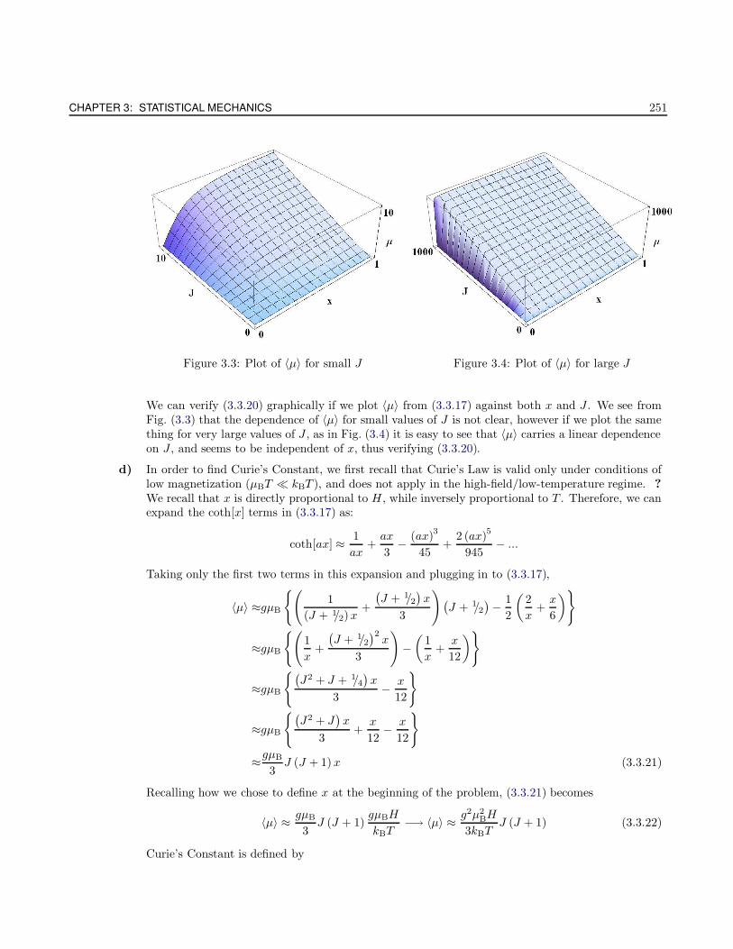
CHAPTER 3: STATISTICAL MECHANICS 251
Figure 3.3: Plot of 〈µ〉 for small J Figure 3.4: Plot of 〈µ〉 for large J
We can verify (3.3.20) graphically if we plot 〈µ〉 from (3.3.17) against both x and J . We see fromFig. (3.3) that the dependence of 〈µ〉 for small values of J is not clear, however if we plot the samething for very large values of J , as in Fig. (3.4) it is easy to see that 〈µ〉 carries a linear dependenceon J , and seems to be independent of x, thus verifying (3.3.20).
d) In order to find Curie’s Constant, we first recall that Curie’s Law is valid only under conditions oflow magnetization (µBT kBT ), and does not apply in the high-field/low-temperature regime. ?We recall that x is directly proportional to H , while inversely proportional to T . Therefore, we canexpand the coth[x] terms in (3.3.17) as:
coth[ax] ≈ 1
ax+ax
3− (ax)
3
45+
2 (ax)5
945− ...
Taking only the first two terms in this expansion and plugging in to (3.3.17),
〈µ〉 ≈gµB
(1
(J + 1/2)x+
(J + 1/2
)x
3
)(J + 1/2
)− 1
2
(2
x+x
6
)
≈gµB
(1
x+
(J + 1/2
)2x
3
)−(
1
x+
x
12
)
≈gµB
(J2 + J + 1/4
)x
3− x
12
≈gµB
(J2 + J
)x
3+
x
12− x
12
≈gµB
3J (J + 1)x (3.3.21)
Recalling how we chose to define x at the beginning of the problem, (3.3.21) becomes
〈µ〉 ≈ gµB
3J (J + 1)
gµBH
kBT−→ 〈µ〉 ≈ g2µ2
BH
3kBTJ (J + 1) (3.3.22)
Curie’s Constant is defined by
W. Erbsen HOMEWORK #3
M =C
TH −→ C = M
T
H(3.3.23)
Where C is Curie’s Constant. Recalling that M = Nµ, and using (3.3.22), we can find Curie’sConstant from (3.3.23) as
C =Ng2µ2
B
3kBJ (J + 1)
Problem 2
Consider a liquid in equilibrium (both thermal and diffusive) with its vapor (treated as an ideal gas). For theliquid, we will apply the following crude model: we treat the liquids as if the molecules still formed a gas ofmolecules moving independently, but with the following considerations. 1) each molecule is assumed to have aconstant potential energy −ε due to its interaction with the other molecules, and 2) each molecule is assumedfree to move throughout a total volume N`v0, where v0 is the average volume available per molecule in the liquidphase.
a) With these assumptions, write down the partition function for a liquid consisting of N` molecules.
b) Now set the chemical potential of the liquid equal to the chemical potential of the vapor phase and find anexpression for the vapor pressure in terms of the temperature and other constants like v0 and ε.
Solution
a) We begin our journey by recalling that the partition function can be expressed in integral form as
QN(N, V, T ) =1
N !h3N
∫∫exp
[−∑N
i Hi
kBT
]dp3N dq3N
N
(3.3.24)
The Hamiltonian, H, in our case is a combination of the kinetic energy term, and the potential energy−ε, which is one of our assumptions in defining our crude model for the liquid. The Hamiltonian isthen given by
H =∑
i
Ti + Vi ⇒N∑
i
p2
i
2m− ε
(3.3.25)
Substituting (3.3.25) into (3.3.24),
Q(`)N (N, V, T ) =
1
N !h3N
∫∫exp
[−∑N
i
p2
i /2m− ε
kBT
]dp3 dq3
N
=1
N !h3N
∫∫exp
[− p2
2mkBT+
ε
kBT
]dp3 dq3
N
=1
N !h3N
exp
[ε
kBT
] ∫exp
[− p2
2mkBT
]dp3
∫dq3N
CHAPTER 3: STATISTICAL MECHANICS 253
=1
N !h3N
V exp
[ε
kBT
][∫ ∞
−∞exp
[− p2
2mkBT
]dp
]3N
=1
N !h3N
V exp
[ε
kBT
] [√2πmkBT
]3N
=1
N !
V exp
[ε
kBT
] [2πmkBT
h2
]3/2N
(3.3.26)
Recalling that the total volume, V , is related to the average volume per molecule, v0, through thenumber of molecules N (`), as V = N (`)v0, and so (3.3.26) becomes
Q(`)N (N, V, T ) =
1
N !
N (`)v0 exp
[ε
kBT
] [2πmkBT
h2
]3/2N
(3.3.27)
b) The chemical potential is given by:
µ ≡(∂F
∂N
)
V,T
≡ −(∂kBT log [Q]
∂N
)
V,T
(3.3.28)
So, let’s find the chemical potential of the liquid first. Substituting (3.3.27) into (3.3.28),
µ(`) = − kBT∂ log
[Q
(`)N
]
∂N
= − kBT∂
∂Nlog
1
N !
Nv0 exp
[ε
kBT
][2πmkBT
h2
]3/2N
= − kBT∂
∂N
log
Nv0 exp
[ε
kBT
] [2πmkBT
h2
]3/2N− log [N !]
= − kBT∂
∂N
N log
[Nv0 exp
[ε
kBT
][2πmkBT
h2
]3/2]− log [N !]
= − kBT
∂
∂N
[N log
[Nv0 exp
[ε
kBT
] [2πmkBT
h2
]3/2]]
︸ ︷︷ ︸I
− ∂
∂Nlog [N !]
︸ ︷︷ ︸II
(3.3.29)
We first evaluate I from (3.3.29):
I =∂
∂N
[N log
[Nv0 exp
[ε
kBT
] [2πmkBT
h2
]3/2]]
= log
[Nv0 exp
[ε
kBT
] [2πmkBT
h2
]3/2]
∂
∂N[N ] +N
∂
∂N
[log
[Nv0 exp
[ε
kBT
] [2πmkBT
h2
]3/2]]
= log
[Nv0 exp
[ε
kBT
] [2πmkBT
h2
]3/2]
+ 1 (3.3.30)
We now carry out the remaining partial derivative in (3.3.29), employing Stirling’s approximation:
W. Erbsen HOMEWORK #3
II =∂
∂Nlog [N !]
=∂
∂NN log [N ] −N
= log [N ]∂
∂NN +N
∂
∂Nlog [N ] − ∂
∂NN
= log [N ] + 1 − 1
= log [N ] (3.3.31)
Substituting (3.3.30) and (3.3.31) back into (3.3.29),
µ(`) = − kBT
log
[Nv0 exp
[ε
kBT
] [2πmkBT
h2
]3/2]
+ 1 − log [N ]
= − kBT
log
[v0 exp
[ε
kBT
] [2πmkBT
h2
]3/2]
+ 1
= − kBT
log
[v0 exp
[ε
kBT
] [2πmkBT
h2
]3/2]
+ log [exp [1]]
= − kBT
log
[v0 exp
[ε
kBT
] [2πmkBT
h2
]3/2
exp [1]
]
= − kBT log
[v0 exp
[ε
kBT+ 1
][2πmkBT
h2
]3/2]
(3.3.32)
In order to find the chemical potential of the gas, we can simply rewrite (3.3.32), where in the newcase ε → 0, and we also recall that v0 = V/N :
µ(g) = −kBT log
[V
N
[2πmkBT
h2
]3/2]
(3.3.33)
Recalling that our gas is in fact an ideal gas, we notice that we can manipulate the ideal gas law as
PV = NkBT −→ V
N=kBT
P(3.3.34)
Substituting (3.3.34) back into (3.3.33),
µ(g) = −kBT log
[kBT
P
[2πmkBT
h2
]3/2]
(3.3.35)
And now, to find the vapor pressure at thermal and diffusive equilibrium, we set µ(`) = µ(g), andfrom (3.3.32) and (3.3.35) we have
−kBT log
[v0 exp
[ε
kBT+ 1
][2πmkBT
h2
]3/2]
= − kBT log
[kBT
P
[2πmkBT
h2
]3/2]
v0 exp
[ε
kBT+ 1
] [2πmkBT
h2
]3/2
=kBT
P
[2πmkBT
h2
]3/2
v0 exp
[ε
kBT+ 1
]=kBT
P(3.3.36)
CHAPTER 3: STATISTICAL MECHANICS 255
We see that (3.3.36) may be trivially solved for P , yielding
P =kBT
v0exp
[−(
ε
kBT+ 1
)]
Problem 3
A zipper has N links, each link has a state in which it is closed with energy 0 and a state in which it is open withenergy ε. We require that the zipper only unzip from the left end, and that the link number s can only open if allthe links to the left(1, s, ..., s− 1) are already open.
a) Show that the partition function can be summed in the form:
QN =1 − e−(N+1)βε
1 − e−βε(3.3.37)
b) Find an expression for the average number of open links at some temperature T .
Solution
a) The standard form of the single-particle partition function is
Q1 =
∞∑
s=0
exp
[− Es
kBT
](3.3.38)
Because the “particles” are distinguishable, then we can gain the full partition from (3.3.38) quiteeasily
Qs =
∞∑
s=0
exp
[− Es
kBT
]s
(3.3.39)
We now take a field trip. Let’s take a close look at the following series:
N∑
s=0
xs = 1 + x+ x2 + x3 + ...+ xN (3.3.40)
We now multiply both sides of (3.3.40) by x. This looks like
x
N∑
s=0
xs = x+ x2 + x3 + x4 + ...+ xN+1 (3.3.41)
We now take (3.3.40) and subtract from it (3.3.41). This yields
(1 − x)
N∑
s=0
xs = 1 − xN+1 (3.3.42)
W. Erbsen HOMEWORK #3
If we were to rearrange (3.3.42), then it would look like
N∑
s=0
xs =1 − xN+1
1 − x(3.3.43)
Noticing that this is the exact sum is what we need in order to evaluate (3.3.39)!
Qs =1 − exp [− (N + 1)Eβ]
1 − exp [−Eβ](3.3.44)
b) In general, the way to find the average number of open links, we use the form
〈s〉 =1
Qs
N∑
s=0
s · exp[−sEβ] (3.3.45)
Now, notice that we can arrive at (3.3.45) if we are very tricky and take a derivative of the followingform:
〈s〉 =1
Qs
∂
∂ (Eβ)
N∑
s=0
exp [−sEβ]
︸ ︷︷ ︸Qs
(3.3.46)
Rewriting (3.3.46) once more,
〈s〉 =1
Qs
∂
∂xQs (3.3.47)
Where I have made the temporary substitution x = Eβ for convenience. Carrying out the firstderivative in (3.3.47),
∂
∂xQs =
∂
∂x
1 − exp [− (N + 1)x]
1 − exp [−x]
=1
1 − exp [−x]
[∂
∂x[1 − exp [− (N + 1)x]]
]+ [1 − exp [− (N + 1)x]]
[∂
∂x
1
1 − exp [−x]
]
=1
1 − exp [−x] [(N + 1) exp [−(N + 1)x]] − [1 − exp [−(N + 1)x]]
[exp [−x]
(1 − exp [−x])2
]
=(N + 1)exp [−(N + 1)x]
1 − exp [−x] − exp [−x][
1 − exp [−(N + 1)x]
(1 − exp [−x])2
]
=(N + 1)exp [−(N + 1)x]
1 − exp [−x] − exp [−x](1 − exp [−x])2
+exp [−x] exp [−(N + 1)x]
(1 − exp [−x])2
=(N + 1)exp [−(N + 1)x]
1 − exp [−x] − 1
1 − exp [−x]
[− exp [−x]
1 − exp [−x] +exp [−(N + 1)x] exp [−x]
1 − exp [−x]
]
=1
1 − exp [−x]
[(N + 1) exp [−(N + 1)x] − exp [−x]
1 − exp [−x] +exp [−(N + 1)x] exp [−x]
1 − exp [−x]
]
=1
1 − exp [−x]
[(N + 1) exp [−(N + 1)x] − exp [−x]
1 − exp [−(N + 1)x]
1 − exp [−x]
](3.3.48)
Where we note that the expression in brackets in (3.3.48) is none other than Qs. Rewriting,
CHAPTER 3: STATISTICAL MECHANICS 257
∂
∂xQs =
1
1 − exp [−x] [(N + 1) exp [−(N + 1)x] − exp [−x]Qs] (3.3.49)
At this point we are ready to substitute (3.3.49) and (3.3.44) into (3.3.47):
〈s〉 =1
Qs· 1
1 − exp [−x] [(N + 1) exp [−(N + 1)x] − exp [−x]Zs]
=(N + 1) exp [−(N + 1)x] − exp [−x]
1 − exp [−x]
=(N + 1) exp [−(N + 1)x]
1 − exp [−x] − exp [−x]1 − exp [−x] (3.3.50)
Putting the numbers back in to (3.3.50) leads us to
〈s〉 =(N + 1) exp [−(N + 1)Eβ]
1 − exp [−Eβ]− exp [−Eβ]
1 − exp [−Eβ](3.3.51)
We are asked to evaluate the average number of open links from (3.3.51) given the following stipu-lation:
E kBT −→ Eβ 1
If Eβ 1, then all the exponential terms approach zero, and so the average number of open linksis
〈s〉 = 0
Problem 4.5
Show that expression (4.3.20) for the entropy of a system in the grand canonical ensemble can also be written as:
S = kB
[∂
∂T(Tq)
]
µ,V
(3.3.52)
Solution
We see that (4.3.20) from Pathria reads
S = kBT
(∂q
∂T
)
z,V
−NkB log [z] + kBq (3.3.53)
We now recall that the differential of the q-potential has the form
dq =
(∂q
∂T
)
z,V
dT +
(∂q
∂V
)
z,T
dV +
(∂q
∂z
)
V,T
dz (3.3.54)
Now that we are inspired, we may now rewrite the partial derivative in (3.3.53) as
W. Erbsen HOMEWORK #3
(∂q
∂T
)
z,V
⇒(∂q
∂T
)
V,T
+
(∂q
∂T
)
µ,V
⇒ ∂q
∂T· ∂T∂z
· ∂z∂T
+
(∂q
∂T
)
µ,V
⇒∂q
∂z· ∂z∂T
+
(∂q
∂T
)
µ,V
(3.3.55)
We now recall (4.3.17), which reads
N(z, V, T )z
[∂
∂zq(z, V, T )
]
V,T
−→(∂q
∂z
)
V,T
=N
z(3.3.56)
Applying (3.3.56) to (3.3.55),
(∂q
∂T
)
z,V
⇒ N
z
∂z
∂T+
(∂q
∂T
)
µ,V
(3.3.57)
Substituting (3.3.57) back into (3.3.53),
S =kBT
N
z
∂z
∂T+
(∂q
∂T
)
µ,V
−NkB log [z] + kBq
=kB
NT
z
∂z
∂T+ T
(∂q
∂T
)
µ,V
−N log [z] + q
(3.3.58)
We now innocently notice that
T
z
∂z
∂T= log [z] (3.3.59)
Accordingly, we can now write (3.3.58) as
S =kB
T
(∂q
∂T
)
µ,V
+ q
=kB
T
(∂q
∂T
)
µ,V
+ q
(∂T
∂T
)
µ,V
−→ S = kB
[∂
∂T(qT )
]
µ,V
Problem 4.8
Determine the grand partition function of a gaseous system of “magnetic” atoms (with J = 1/2 and g = 2)which can have, in addition to the kinetic energy, a magnetic potential energy equal to µBH or −µBH , dependingupon their orientation with respect to the applied magnetic field H . Derive an expression for the magnetization ofthe system, and calculate how much heat will be given off by the system when the magnetic field is reduced fromH to zero at constant volume and constant temperature.
CHAPTER 3: STATISTICAL MECHANICS 259
Solution
The (canonical) single-particle partition function is defined by
Q1 =1
h3
∫∫exp
[∑Ni Hi
kBT
]d3p d3q (3.3.60)
The Hamiltonian in this case is
H =p2
2m± µBH (3.3.61)
Applying (3.3.61) to (3.3.60),
Q1 =1
h3
∫∫exp
[p2/2m± µBH
kBT
]d3p d3q
=1
h3
∫∫exp
[p2
2mkBT± µBH
kBT
]d3p d3q
=1
h3exp
[±µBH
kBT
] ∫d3q
∫exp
[p2
2mkBT
]d3p
=V
h3exp
[±µBH
kBT
]∫ ∞
−∞exp
[p2
2mkBT
]dp
3
=V
h3exp
[±µBH
kBT
]√2πmkBT
3
(3.3.62)
We now notice that the exponential term can be rewritten as
exp
[±µBH
kBT
]=exp
[+µBH
kBT
]+ exp
[−µBH
kBT
]⇒ 2 cosh
[−µBH
kBT
](3.3.63)
Substituting (3.3.63) back into (3.3.62),
Q1 =2V
h3cosh
[−µBH
kBT
][2πmkBT ]
3/2 (3.3.64)
Using (3.3.64), we can now say that the full partition function is
QN =1
N !
2V
h3cosh
[−µBH
kBT
][2πmkBT ]
3/2
N
(3.3.65)
We now recall that the equation linking the grand partition function to the canonical partition functionis
Q =
∞∑
N=0
zNQN (3.3.66)
Where z is the fugacity. Substituting (3.3.65) into (3.3.66),
Q =
∞∑
N=0
zN 1
N !
2V
h3cosh
[−µBH
kBT
][2πmkBT ]
3/2
N
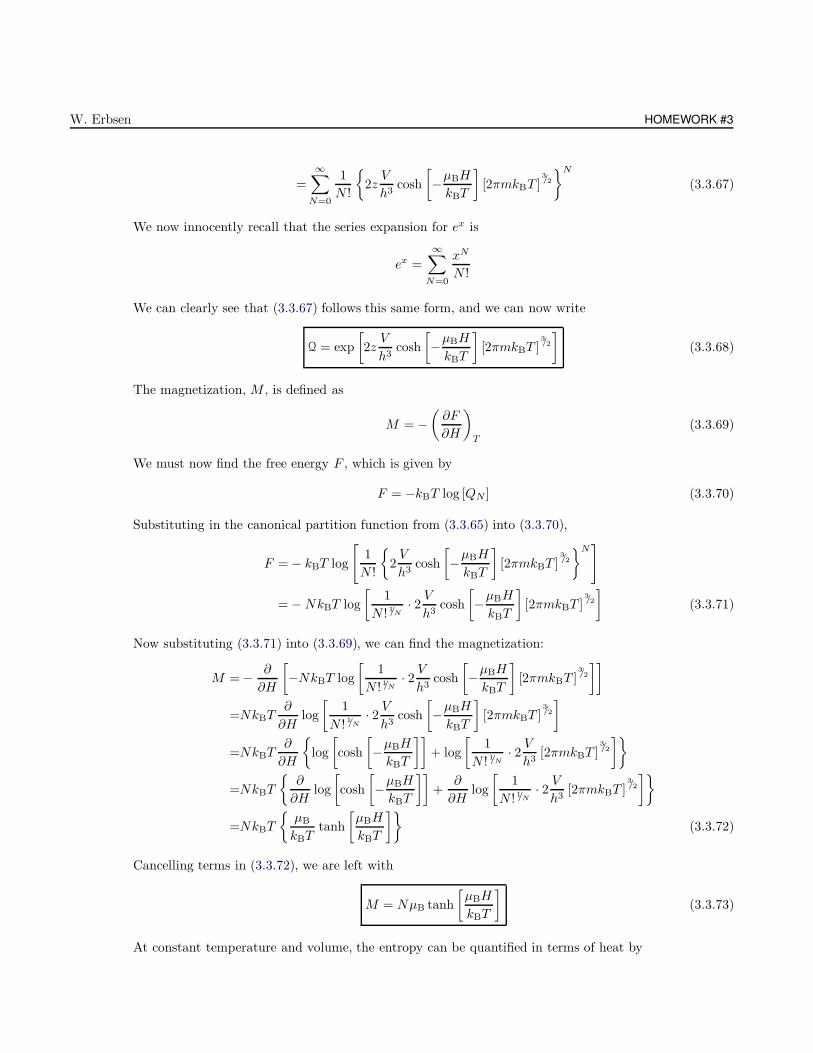
W. Erbsen HOMEWORK #3
=
∞∑
N=0
1
N !
2zV
h3cosh
[−µBH
kBT
][2πmkBT ]
3/2
N
(3.3.67)
We now innocently recall that the series expansion for ex is
ex =
∞∑
N=0
xN
N !
We can clearly see that (3.3.67) follows this same form, and we can now write
Q = exp
[2zV
h3cosh
[−µBH
kBT
][2πmkBT ]
3/2
](3.3.68)
The magnetization, M , is defined as
M = −(∂F
∂H
)
T
(3.3.69)
We must now find the free energy F , which is given by
F = −kBT log [QN ] (3.3.70)
Substituting in the canonical partition function from (3.3.65) into (3.3.70),
F = − kBT log
[1
N !
2V
h3cosh
[−µBH
kBT
][2πmkBT ]
3/2
N]
= −NkBT log
[1
N ! 1/N· 2 Vh3
cosh
[−µBH
kBT
][2πmkBT ]
3/2
](3.3.71)
Now substituting (3.3.71) into (3.3.69), we can find the magnetization:
M = − ∂
∂H
[−NkBT log
[1
N ! 1/N· 2 Vh3
cosh
[−µBH
kBT
][2πmkBT ]
3/2
]]
=NkBT∂
∂Hlog
[1
N !1/N
· 2 Vh3
cosh
[−µBH
kBT
][2πmkBT ]
3/2
]
=NkBT∂
∂H
log
[cosh
[−µBH
kBT
]]+ log
[1
N ! 1/N· 2 Vh3
[2πmkBT ]3/2
]
=NkBT
∂
∂Hlog
[cosh
[−µBH
kBT
]]+
∂
∂Hlog
[1
N ! 1/N· 2 Vh3
[2πmkBT ]3/2
]
=NkBT
µB
kBTtanh
[µBH
kBT
](3.3.72)
Cancelling terms in (3.3.72), we are left with
M = NµB tanh
[µBH
kBT
](3.3.73)
At constant temperature and volume, the entropy can be quantified in terms of heat by
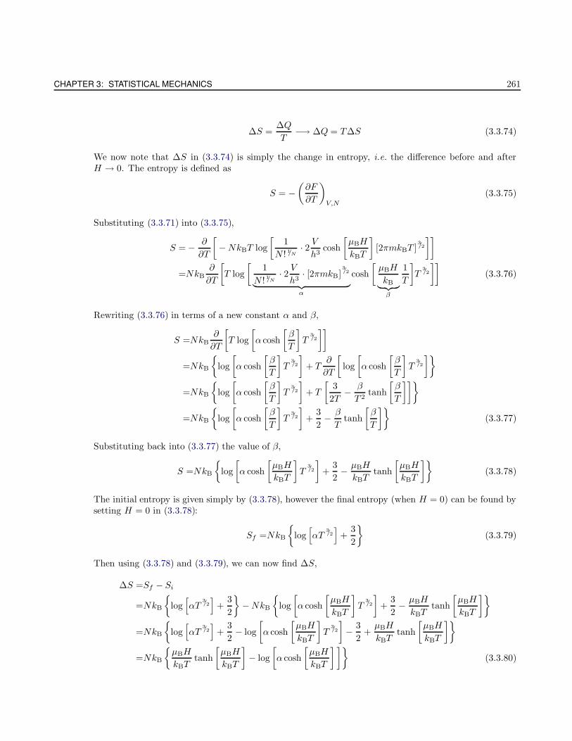
CHAPTER 3: STATISTICAL MECHANICS 261
∆S =∆Q
T−→ ∆Q = T∆S (3.3.74)
We now note that ∆S in (3.3.74) is simply the change in entropy, i.e. the difference before and afterH → 0. The entropy is defined as
S = −(∂F
∂T
)
V,N
(3.3.75)
Substituting (3.3.71) into (3.3.75),
S = − ∂
∂T
[−NkBT log
[1
N ! 1/N· 2 Vh3
cosh
[µBH
kBT
][2πmkBT ]
3/2
]]
=NkB∂
∂T
[T log
[1
N !1/N
· 2 Vh3
· [2πmkB]3/2
︸ ︷︷ ︸α
cosh
[µBH
kB︸ ︷︷ ︸β
1
T
]T
3/2
]](3.3.76)
Rewriting (3.3.76) in terms of a new constant α and β,
S =NkB∂
∂T
[T log
[α cosh
[β
T
]T
3/2
]]
=NkB
log
[α cosh
[β
T
]T
3/2
]+ T
∂
∂T
[log
[α cosh
[β
T
]T
3/2
]
=NkB
log
[α cosh
[β
T
]T
3/2
]+ T
[3
2T− β
T 2tanh
[β
T
]]
=NkB
log
[α cosh
[β
T
]T
3/2
]+
3
2− β
Ttanh
[β
T
](3.3.77)
Substituting back into (3.3.77) the value of β,
S =NkB
log
[α cosh
[µBH
kBT
]T
3/2
]+
3
2− µBH
kBTtanh
[µBH
kBT
](3.3.78)
The initial entropy is given simply by (3.3.78), however the final entropy (when H = 0) can be found bysetting H = 0 in (3.3.78):
Sf =NkB
log[αT
3/2]
+3
2
(3.3.79)
Then using (3.3.78) and (3.3.79), we can now find ∆S,
∆S =Sf − Si
=NkB
log[αT
3/2]
+3
2
−NkB
log
[α cosh
[µBH
kBT
]T
3/2
]+
3
2− µBH
kBTtanh
[µBH
kBT
]
=NkB
log[αT
3/2]
+3
2− log
[α cosh
[µBH
kBT
]T
3/2
]− 3
2+µBH
kBTtanh
[µBH
kBT
]
=NkB
µBH
kBTtanh
[µBH
kBT
]− log
[α cosh
[µBH
kBT
] ](3.3.80)
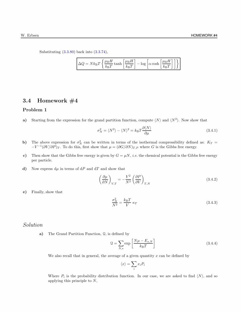
W. Erbsen HOMEWORK #4
Substituting (3.3.80) back into (3.3.74),
∆Q = NkBT
µBH
kBTtanh
[µBH
kBT
]− log
[α cosh
[µBH
kBT
] ]
3.4 Homework #4
Problem 1
a) Starting from the expression for the grand partition function, compute 〈N〉 and 〈N2〉. Now show that
σ2N = 〈N2〉 − 〈N〉2 = kBT
∂〈N〉∂µ
(3.4.1)
b) The above expression for σ2N can be written in terms of the isothermal compressibility defined as: KT =
−V −1(∂V/∂P )T . To do this, first show that µ = (∂G/∂N)T,P where G is the Gibbs free energy.
c) Then show that the Gibbs free energy is given by G = µN , i.e. the chemical potential is the Gibbs free energyper particle.
d) Now express dµ in terms of dP and dT and show that
(∂µ
∂N
)
V,T
= − V 2
N2
(∂P
∂V
)
T,N
(3.4.2)
e) Finally, show that
σ2N
N2=kBT
VκT (3.4.3)
Solution
a) The Grand Partition Function, Q, is defined by
Q =∑
N,s
exp
[Nµ−Es,N
kBT
](3.4.4)
We also recall that in general, the average of a given quantity x can be defined by
〈x〉 =∑
i
xiPi
Where Pi is the probability distribution function. In our case, we are asked to find 〈N〉, and soapplying this principle to N ,
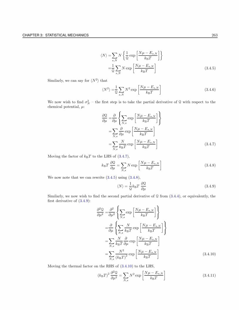
CHAPTER 3: STATISTICAL MECHANICS 263
〈N〉 =∑
s,N
N
1
Qexp
[Nµ− Es,N
kBT
]
=1
Q
∑
s,N
N exp
[Nµ− Es,N
kBT
](3.4.5)
Similarly, we can say for 〈N2〉 that
〈N2〉 =1
Q
∑
s,N
N2 exp
[Nµ −Es,N
kBT
](3.4.6)
We now wish to find σ2N – the first step is to take the partial derivative of Q with respect to the
chemical potential, µ:
∂Q
∂µ=∂
∂µ
∑
N,s
exp
[Nµ− Es,N
kBT
]
=∑
N,s
∂
∂µexp
[Nµ− Es,N
kBT
]
=∑
N,s
N
kBTexp
[Nµ−Es,N
kBT
](3.4.7)
Moving the factor of kBT to the LHS of (3.4.7),
kBT∂Q
∂µ=∑
N,s
N exp
[Nµ −Es,N
kBT
](3.4.8)
We now note that we can rewrite (3.4.5) using (3.4.8),
〈N〉 =1
QkBT
∂Q
∂µ(3.4.9)
Similarly, we now wish to find the second partial derivative of Q from (3.4.4), or equivalently, thefirst derivative of (3.4.9):
∂2Q
∂µ2=∂2
∂µ2
∑
N,s
exp
[Nµ− Es,N
kBT
]
=∂
∂µ
∑
N,s
N
kBTexp
[Nµ− Es,N
kBT
]
=∑
N,s
N
kBT
∂
∂µexp
[Nµ −Es,N
kBT
]
=∑
N,s
N2
(kBT )2 exp
[Nµ− Es,N
kBT
](3.4.10)
Moving the thermal factor on the RHS of (3.4.10) to the LHS,
(kBT )2 ∂
2Q
∂µ2=∑
N,s
N2 exp
[Nµ− Es,N
kBT
](3.4.11)
W. Erbsen HOMEWORK #4
Using (3.4.11), we can rewrite (3.4.6),
〈N2〉 =1
Q(kBT )2
∂2Q
∂µ2(3.4.12)
Substituting (3.4.9) and (3.4.12) into (3.4.1),
σ2N =〈N2〉 − 〈N〉2
=1
Q(kBT )
2 ∂2Q
∂µ2−
1
QkBT
∂Q
∂µ
2
=1
Q(kBT )2
∂2Q
∂µ2− 1
Q2(kBT )2
(∂Q
∂µ
)2
=kBT
Q
[kBT
∂2Q
∂µ2− 1
QkBT
(∂Q
∂µ
)2]
=kBT
Q
[kBT
∂2Q
∂µ2− 1
QkBT
∂Q
∂µ︸ ︷︷ ︸·∂Q∂µ
](3.4.13)
Noticing that the underbraced term in (3.4.13) is 〈N〉 from (3.4.9),
σ2N =
kBT
Q
[kBT
∂2Q
∂µ2− 〈N〉∂Q
∂µ
]
=kBT
Q
[∂
∂µ· kBT
∂Q
∂µ︸ ︷︷ ︸−〈N〉∂Q
∂µ
](3.4.14)
Solving (3.4.5) for the underbraced term in (3.4.14) and making the substitution,
σ2N =
kBT
Q
[∂
∂µ(Q〈N〉) − 〈N〉∂Q
∂µ
](3.4.15)
We not notice that the first partial derivative may be carried out to be
∂
∂µ(Q〈N〉) = Q
∂〈N〉∂µ
+ 〈N〉∂Q∂µ
(3.4.16)
Substituting (3.4.16) back into (3.4.15), we find that
σ2N =
kBT
Q
[Q∂〈N〉∂µ
+ 〈N〉∂Q∂µ
− 〈N〉∂Q∂µ
]−→ σ2
N = kBT∂〈N〉∂µ
(3.4.17)
b) To show that we can write the chemical potential in terms of the Gibbs Free Energy as suggestedin the prompt, we first recall that the Gibbs Free Energy is defined by (1.3.15) as
G = E − TS + PV ⇒ µN (3.4.18)
Where the RHS can be used if the intensive parameters T , p, and µ remain constant while theextensive parameters N , V , and E grow proportionately with one another (See Footnote 8 on pg.28). Therefore, the chemical potential can be defined in terms of the Gibbs Free Energy as
µ =
(∂G
∂N
)
T,P
(3.4.19)
CHAPTER 3: STATISTICAL MECHANICS 265
c) Recalling that the non-differential analogue to (1.3.4) reads
E = TS − PV + µN (3.4.20)
Substituting (3.4.20) into the LHS of (3.4.18), we see that
G = (TS − PV + µN) − TS + PV −→ G = µN (3.4.21)
d) Extending the Gibbs Free Energy to a multi-particle system, we can find the differential as
dG = µdN +Ndµ (3.4.22)
We also note that the differential of G from (3.4.18) is
dG = −SdT + V dP + µdN (3.4.23)
Equating (3.4.22) and (3.4.23), we find that
µdN +Ndµ = −SdT + V dP + µdN −→ dµ = − S
NdT +
V
NdP (3.4.24)
Letting dT → 0, (3.4.24) becomes
dµ =V
NdP −→ ∂µ
∂P=V
N(3.4.25)
Applying the chain rule to (3.4.25),
∂µ
∂P
∂P
∂V
∂V
∂P=V
N−→ ∂µ
∂V
∂V
∂P=V
N−→ ∂µ
∂V=V
N
∂P
∂V(3.4.26)
Applying the chain rule once again to the LHS of (3.4.26),
∂µ
∂V
∂V
∂N
∂N
∂V=V
N
∂P
∂V
∂µ
∂N−→ ∂N
∂V=V
N
∂P
∂V(3.4.27)
We now note that from Maxwell’s relations, we can write(∂N
∂V
)
T,µ
=
(∂P
∂µ
)
T,V
(3.4.28)
Substituting (3.4.28) into (3.4.27),(∂µ
∂N
)
T,V
(∂P
∂µ
)
T,V
=V
N
(∂P
∂V
)
T,N
(3.4.29)
From a previous homework set, we were asked to establish
−N = V
(∂P
∂µ
)
T,V
−→(∂P
∂µ
)
T,V
= −NV
(3.4.30)
Substituting (3.4.32) into (3.4.31),
(∂µ
∂N
)
T,V
N
V= − V
N
(∂P
∂V
)
T,N
−→(∂µ
∂N
)
T,V
= − V 2
N2
(∂P
∂V
)
T,N
(3.4.31)
W. Erbsen HOMEWORK #4
e) The first thing we must do is recognize that the isothermal compressibility, κT , can be quantifiedas
κT = − 1
V
(∂V
∂P
)
T,N
(3.4.32)
For a system being isothermally compressed (both T and N constant), we note that we can rewrite(3.4.31) as
(∂µ
∂N
)
T,V
= − V 2
N2
(∂P
∂V
)
T,N
−→(∂〈N〉∂µ
)
T,V
= − N2
V 2
(∂V
∂P
)
T,N
=N2
V
[− 1
V
(∂V
∂P
)
T,N
](3.4.33)
Substituting (3.4.32) into the RHS of (3.4.33),(∂〈N〉∂µ
)
T,V
=N2
VκT −→ kBT
(∂〈N〉∂µ
)
T,V
= kBTN2
VκT (3.4.34)
Substituting (3.4.1) into (3.4.34) and rearranging, we see that
σ2N = kBT
N2
VκT −→ σ2
N
N2=kBT
VκT
Which is the same as (3.4.3).
Problem 2
A surface with N adsorption sites is in equilibrium with a mixed ideal gas containing molecules of type A and B.Each site can take either one single A molecules with energy −εA or a single B molecule with energy −εB . Com-pute the grand canonical partition function for this adsorbed system. Then find relations between the fractionaloccupations (θA = nA/N and θB = nB/N) and the partial pressures pA and pB.
Solution
Recalling that the Grand Canonical Partition Function (i.e. the Gibbs Sum) is given by
Q =∑
N,s
exp
[µsN −Es,N
kBT
](3.4.35)
In order to find the PT for the adsorbed system, we assume that there are only two states available tothe system, one where molecule A is adsorbed and the other where molecule B is adsorbed. There is nostate where neither molecule is connected - this is deduced from the wording of the problem. We recallthat the Grand PT can be defined in terms of the canonical PT from (4.3.15) as
Q =∑
n
znQn (3.4.36)
CHAPTER 3: STATISTICAL MECHANICS 267
Where z is the fugacity (= eµs/kBT ) and Qn is the canonical PT. Following the example in class of a gasadsorbed onto a lattice, , we note that the canonical PT with degeneracy is
Qn = gn · exp
[−Es,n
kBT
]n
(3.4.37)
Where the degeneracy is
gN =N(N − 1)...(N − n+ 1)
n!⇒ N !
(N − n)!n!(3.4.38)
Substituting (3.4.38) into (3.4.37),
Qn =N !
(N − n)!n!exp
[−Es,n
kBT
]n
(3.4.39)
And now substituting (3.4.39) back into the Grand PT from (3.4.36),
Q =∑
n,s
exp
[µs
kBT
]· N !
(N − n)!n!exp
[−Es,n
kBT
]n
=∑
n,s
N !
(N − n)!n!exp
[(µs − Es,n)n
kBT
](3.4.40)
Using the Binomial Expansion, (3.4.40) becomes,
Q =∑
s
1 + exp
[µs −Es
kBT
]N
(3.4.41)
In our case, since we have two possible energies, the sum is carried out to A and B and hence has onlytwo terms. We now see that (3.4.41) becomes
Q =
1 + exp
[(µA + εA)
kBT
]+ exp
[(µB + εB)
kBT
]N
(3.4.42)
We now recall from class that the thermodynamic potential, Φ, is defined in terms of the Grand CanonicalPT as
Φ = −kBT log [Q] (3.4.43)
Substituting (3.4.36) into (3.4.43),
Φ = −kBT log
[∑
n
znQn
]⇒ −kBT log [Q] (3.4.44)
We can now take the partial derivative of (3.4.44) with respect to µ, which yields
−∂Φ∂µ
= z∂
∂zlog [Q] (3.4.45)
Noticing that the RHS of (3.4.45) is equal to n, or the average number of adsorbed molecules, we nowcan say

W. Erbsen HOMEWORK #4
n = −∂Φ∂µ
(3.4.46)
Substituting the thermodynamic potential from (3.4.44) into (3.4.46),
n = − ∂
∂µ−kBT log [Q] (3.4.47)
At this point, we remember that it is important to be very careful, as both n and µ are a function of thespecific states in the Gibbs sum. Rewriting (3.4.48) to make this more explicit,
ns = − kBT∂
∂µslog [Q] (3.4.48)
And now substituting the grand canonical PT from (3.4.42) into (3.4.48),
ns = − kBT∂
∂µslog
[1 + exp
[(µA + εA)
kBT
]+ exp
[(µB + εB)
kBT
]N]
= −NkBT∂
∂µslog
[1 + exp
[(µA + εA)
kBT
]+ exp
[(µB + εB)
kBT
]](3.4.49)
We can go no further until we explicitly define which state we are evaluating ns for. Starting with A,(3.4.49) becomes
nA =NkBT∂
∂µAlog
[1 + exp
[(µA + εA)
kBT
]+ exp
[(µB + εB)
kBT
]]
=N
β
∂
∂µAlog [1 + exp [(µA + εA)β] + exp [(µB + εB)β]]
=N
β
β
exp [(µA + εA)β]
1 + exp [(µA + εA)β] + exp [(µB + εB)β]
=Nexp [(µA + εA)β]
1 + exp [(µA + εA)β] + exp [(µB + εB)β](3.4.50)
The average number of adsorbed molecules per site is given by θs = ns/N , and we are of course interestedin the fractional coverage of each type of molecule to each site. Accordingly, θA can be found from (3.4.50)to be
θA =exp [(µA + εA)β]
1 + exp [(µA + εA)β] + exp [(µB + εB)β](3.4.51)
And similarly, for θB ,
θB =exp [(µB + εB)β]
1 + exp [(µA + εA)β] + exp [(µB + εB)β](3.4.52)
The time has now come to find the partial pressure pA and pB . The first step is to isolate µ from θin either (3.4.51) or (3.4.52). Following the example from lecture, we first wish to find the chemicalpotential of the surface (µsurf), and equate it with the chemical potential of the gas (µgas). Starting withµsurf, we recognize that µA = µB ⇒ µ, and also θA = θB ⇒ θ, and so
CHAPTER 3: STATISTICAL MECHANICS 269
1
θ=
1 + exp [(µsurf + εA)β] + exp [(µsurf + εB)β]
exp [(µsurf + εA)β]
=1
exp [(µsurf + εA)β]+
exp [(µsurf + εA)β]
exp [(µsurf + εA)β]+
exp [(µsurf + εB)β]
exp [(µsurf + εA)β]
=1 +1
exp [(µsurf + εA)β]+ exp [(εB − εA)β] (3.4.53)
If we define ∆ε = εB − εB, then (3.4.53) becomes
exp [− (µsurf + εA)β] =1
θ− 1 − exp [∆εβ] −→ µsurf = − 1
βlog
[1
θ− 1 − exp [∆εβ]
]− εA (3.4.54)
From class, we know that the chemical potential of an ideal gas is given, in general by
µgas =1
βlog [P · f(T )] (3.4.55)
Equating (3.4.54) and (3.4.56),
− 1
βlog
[1
θ− 1 − exp [∆εβ]
]− εA =
1
βlog [P · f(t)]
log
[1
θ− 1 − exp [∆εβ]
]+ εAβ = log
[1
P · f(t)
]
(1
θ− 1 − exp [∆εβ]
)exp [εAβ] =
1
P · f(t) (3.4.56)
Recalling that ∆ε = εB − εA, (3.4.56) becomes(
1 − θ
θ
)exp [εAβ] − exp [εBβ] =
1
P · f(t) −→ P =1
f(T )
(θ
1 − θ
)1
exp [εAβ] − exp [εBβ](3.4.57)
If we assume that the total gas mixture is given by P from (3.4.57), then the partial pressure is definedby pi = niP . To find nA, we follow this logic and from (3.4.50) and (3.4.57), we can find pA:
pA = Nexp [(µA + εA)β]
1 + exp [(µA + εA)β] + exp [(µB + εB)β]· 1
f(T )
(θ
1 − θ
)1
exp [εAβ] − exp [εBβ](3.4.58)
And similarly, we can say that the partial pressure of molecule B is given by
pB = Nexp [(µB + εB)β]
1 + exp [(µA + εA)β] + exp [(µB + εB)β]· 1
f(T )
(θ
1 − θ
)1
exp [εAβ] − exp [εBβ](3.4.59)
It might be possible to reduce (3.4.58)–(3.4.59) to a slightly nicer form, however it will likely still bequite ugly.
Problem 3
W. Erbsen HOMEWORK #4
Suppose that N molecules of H2O gas (assumed to behave like a classical ideal gas) are introduces into a containerof fixed volume V at a temperature low enough that virtually all the gas remains as molecular water vapor. Athigher temperatures dissociation can take place according to the reaction
2H2O 2H2 + O2 (3.4.60)
Let x be the fraction of H2O molecules dissociated at some temperature T corresponding to the total gas pressureP . Write an equation relating x, P , and F (t) where F (t) is some function of temperature (that can include thebinding energy of the water molecule).
Solution
The dynamic reaction in (3.4.60) can be rewritten as
2H2O − 2H2 − O2 = 0 (3.4.61)
We can express (3.4.61) in terms of coefficients and species according to∑
i aiAi, and in our case thecoefficients are
A1 = H2, A2 = O2, A3 = H2Oa1 = −2, a2 = −1, a3 = 2
We also recall that the condition for chemical equilibrium can be defined in terms of the coefficients ai
as
∑
i
aiµi = 0 (3.4.62)
Where this condition is met at the equilibrium pressure and temperature. We can express (3.4.61) inthe language of (3.4.62) as
2µ (H2O) − 2µ (H2) − µ (O2) = 0 (3.4.63)
The chemical potential for each species, µi, can be described by (1.5.7), which reads
µi(Ni, V, T ) = kBT log
Ni
V
(h2
2πmikBT
) 3/2
(3.4.64)
We now define the fractional occupancy Ni, which we quantify as N ′i = Ni/N . If we assume that the
gas phase of each species can be treated as ideal, then we can write PV = NkBT → N/V = P/ (kBT ),and we can rewrite (3.4.64) as
µi(Ni, V, T ) =kBT log
[P
kBTN ′
i
(h2
2πmikBT
) 3/2]
=kBT log
[P
kBT
(h2
2πmikBT
)3/2]
+ kBT log [N ′i ] (3.4.65)
Using (3.4.62), we may rewrite (3.4.65) as
CHAPTER 3: STATISTICAL MECHANICS 271
kBT∑
i
ai
log
[P
kBT
(h2
2πmikBT
) 3/2]
+ log [N ′i ]
= 0 (3.4.66)
Killing the factor in front of the sum and rearranging, (3.4.66) becomes
−∑
i
ai log
[P
kBT
(h2
2πmikBT
) 3/2]
=∑
i
ai log [N ′i ]
∑
i
log
[kBT
P
(2πmikBT
h2
) 3/2]ai
=∑
i
log [N ′i ]
ai
∑
i
log
[V
Ni
(2πmikBT
h2
) 3/2]ai
=∑
i
log [N ′i ]
ai
∑
i
log
[qi
Ni
]ai
=∑
i
log [N ′i ]
ai (3.4.67)
From lecture, we know that
Na11 ·Na2
2 ·Na33 · ... = qa1
1 · qa22 · qa3
3 · ...⇒ K(T, V ) (3.4.68)
And, simply by visual inspection of (3.4.67), we can see that K(T, V ) = qai
i makes sense, recognizingthat at equilibrium
∑iKi(T, V ) = 1 so the equation reduces readily to 0 = 0. We now recall that we
can alternatively define the equilibrium constant in terms of (3.4.60) as
K(T, V ) =[H2O]
2
[H2]2[O2]
⇒ N (H2O)2
N (H2)2 N (O2)(3.4.69)
We also recall from lecture that
∏
i
Ni
qi
ai
= 1 (3.4.70)
Applying (3.4.70) to the case of (3.4.60),
NH2O
qH2O
2
·NH2
qH2
−2
·NO2
qO2
−1
=1 (3.4.71)
The total number of species at any time, ΣN ′, can be quantified by
ΣN ′ = NH2O +NH2 +NO2 (3.4.72)
We are told to let x denote the fraction of water molecules dissociated after some period of time, and alsothat initially, the total number of free particulates are entirely water molecules, so that ΣN = NH2O.Accordingly, we see that in my notation x = 1 −NH2O/ΣN . With this, (3.4.72) becomes
ΣN ′ = ΣN (1 − x) +NH2+NO2
(3.4.73)
Following the same logic, we see that NH2 grows proportionally with NH2O, whereas NO2 grows half -proportionally with respect to NH2O (according to the stoichiometric coefficients from (3.4.60)). We seethat (3.4.73) becomes
W. Erbsen HOMEWORK #4
ΣN ′ = ΣN (1 − x) + xΣN + xΣN
2−→ 1 =
ΣN
ΣN ′ (1 − x) +ΣN
ΣN ′ x+ΣN
ΣN ′x
2(3.4.74)
Substituting the appropriate fractional coefficients into (3.4.71),
ΣN (1 − x)
qH2O
2
I
·xΣN
qH2
−2
II
·
1/2xΣN
qO2
−1
III
=1 (3.4.75)
We now recall that qi is defined by
qi =pi
kBT· Ppi
· pi
P
(h2
2πmikBT
)3/2
=P
kBT
Ni
ΣN
(h2
2πmikBT
) 3/2
=P
m3/2i
Ni
ΣN
(h2
2π (kBT )3
)3/2
︸ ︷︷ ︸F (T )
−→ qi =Ni
ΣN· P
m3/2i
F (T ) (3.4.76)
In the language of (3.4.76), we can rewrite each of the terms in (3.4.75). Starting with I,
I =
ΣN (1 − x)
qH2O
2
=
(1 − x) ·
m3/2H2O
F (T )P
2
=(1 − x)2 ·
m3H2O
[F (T )P ]2 (3.4.77a)
II =
xΣN
qH2
−2
=
x ·
m3/2H2
F (T )P
−2
=
x2 ·
m3H2
[F (T )P ]2
−1
=1
x2· [F (T )P ]
2
m3H2
(3.4.77b)
III =
1/2xΣN
qO2
−1
=
x
2·m
3/2O2
F (T )P
−1
CHAPTER 3: STATISTICAL MECHANICS 273
=2
x· F (T )P
m3/2O2
(3.4.77c)
Substituting (3.4.77a)–(3.4.77c) back into (3.4.75),
(1 − x)
2 ·m3
H2O
[F (T )P ]2
·
1
x2· [F (T )P ]
2
m3H2
2
x· F (T )P
m3/2O2
=1
(1 − x)2
x3· 2(
m2H2O
m2H2mO2
) 3/2
F (T )P =1 (3.4.78)
Rearranging (3.4.78), we are left with
F (T )P =x3
2 (1 − x)2
(m2
H2mO2
m2H2O
) 3/2
Problem 4
Evaluate the density matrix ρmn of an electron spin in the representation which makes σx diagonal. Next, showthat the value of 〈σz〉, resulting from this representation, is precisely the same as the one obtained in 5.3. Hint :the representation needed here follows from the one used in 5.3 by carrying out a transformation with the helpof the unitary operator
U =
(1/
√2 1/
√2
−1/√
2 1/√
2
)(3.4.79)
Solution
The Pauli spin matrices are given by
σx =
(0 11 0
), σy =
(0 −ii 0
), σz =
(1 00 −1
)
We now note that we can straightforwardly rewrite our unitary operator from (3.4.79) as
U =1√2
(1 1
−1 1
)(3.4.80)
We also recognize that by using this matrix, we may transform our spin matrices to a basis in which σx
is diagonal via a unitary transformation:
σ′x = U
†σxU (3.4.81)
Where σ′x denotes σx in the basis in which it is diagonal. Substituting (3.4.80) into (3.4.81),
W. Erbsen HOMEWORK #4
σ′x =
1√2
(1 1
−1 1
)†(0 11 0
)1√2
(1 1
−1 1
)
=1
2
(1 −11 1
)(0 11 0
)(1 1
−1 1
)
=1
2
(1 1
−1 1
)(1 1
−1 1
)
=1
2
(−2 0
0 2
)
=
(−1 0
0 1
)(3.4.82)
So, the provided matrix does indeed diagonalize σx. We must now see how it affects σz,
σ′z =
1√2
(1 1
−1 1
)†(1 00 −1
)1√2
(1 1
−1 1
)
=1
2
(1 −11 1
)(1 00 −1
)(1 1
−1 1
)
=1
2
(1 11 −1
)(1 1
−1 1
)
=1
2
(0 22 0
)
=
(0 11 0
)(3.4.83)
The Hamiltonian operator, H, is given by (5.3.1),
H = −µBBσ′z (3.4.84)
Which includes our new Pauli Matrix σ′z in the basis in which σx is diagonal. Substituting (3.4.83) into
(3.4.84),
H = −µBB
(0 11 0
)(3.4.85)
We now recall the expression for the density matrix in the canonical ensemble is given by (5.3.3) as
(ρ) =
(e−βH
)
Tr(e−βH
)
=1
eβµBB + e−βµBB
(eβµBB 0
0 e−βµBB
)(3.4.86)
But this is not the answer. We must now express this density matrix in our new basis, in the same waywe did with our Pauli spin matrices before. Performing the unitary transformation on (3.4.86),
CHAPTER 3: STATISTICAL MECHANICS 275
(ρ′) =1√2
(1 1
−1 1
)†1
eβµBB + e−βµBB
(eβµBB 0
0 e−βµBB
)1√2
(1 1
−1 1
)
=1
2
1
eβµBB + e−βµBB
(1 −11 1
)(eβµBB 0
0 e−βµBB
)(1 1
−1 1
)
=1
2
1
eβµBB + e−βµBB
(eβµBB −e−βµBB
eβµBB e−βµBB
)(1 1
−1 1
)
=1
eβµBB + e−βµBB
(eβµBB + e−βµBB eβµBB − e−βµBB
eβµBB − e−βµBB eβµBB + e−βµBB
)
=1
2 cosh [βµBB]
(cosh [βµBB] sinh [βµBB]sinh [βµBB] cosh [βµBB]
)(3.4.87)
We may now absorb the cosh term out front of (3.4.87) to inside the matrix, leaving us with
(ρ′) =1
2
(1 tanh [βµBB]
tanh [βµBB] 1
)(3.4.88)
We can find the expectation value of σ′x by generalizing the form of (5.3.4),
〈σ′x〉 = Tr [ρ′σ′] (3.4.89)
Substituting σ′z from (3.4.83) and ρ′ from (3.4.88) into (3.4.89),
〈σ′x〉 =Tr
[1
2
(1 tanh [βµBB]
tanh [βµBB] 1
)(0 11 0
)]
=Tr
[1
2
(tanh [βµBB] 1
1 tanh [βµBB]
)](3.4.90)
Recalling that the trace of a matrix is simply the sum of the diagonal elements, (3.4.90) becomes
〈σ′x〉 = tanh [βµBB]
Which is the same as found in 5.3.
3.5 Homework #7
Problem 1
Extension of the Debye Model of a Solid: Assuming the dispersion relation ω = Aks, where ω is the angularfrequency and k is the wave-number of a vibrational mode existing in a solid, show that the respective contribu-tion towards the specific heat of the solid at low temperature is proportional to T
3/s .
W. Erbsen HOMEWORK #7
Solution
This problem is essentially the same as if we were trying to find the specific heat of a Debye solid atlow temperatures, the only difference is that the dispersion relation has an extra term s in the exponentof the wave-number: ω = Aks. We can carry through the arithmatic in very much the same way then,following Pathria’s work in 7.2 and 7.3.
We first recall that the specific heat in terms of internal energy is given by
CV (T ) =
(∂U
∂T
)
V
(3.1.1)
So our goal then, is to find the internal energy, U , as a function of our dispersion relation. We recallPathria’s definition of the Debye function from (7.3.18):
D(x0) =3
x30
∫ x0
0
x3
ex − 1dx (3.1.2)
Where we have defined x0 to be
x0 =~ωD
kBT(3.1.3)
And substituting (3.1.3) back into (3.1.2),
D(x0) = 3
(kBT
~ωD
)3 ∫ x0
0
x3
ex − 1dx (3.1.4)
We also realize that, to make things more transparent, Pathria has made the substitution x = ~ωE/kBT .Recalling our definition of x0 from (3.1.3), we note that in the low temperature limit, as suggested inthe prompt, we see that x0 ∼ 1/T → ∞, and so (3.1.4) becomes
D(x0) =3
(kBT
~ωD
)3 ∫ ∞
0
x3
ex − 1dx
=3
(kBT
~ωD
)3 [π4
15
](3.1.5)
The only difference in our case is that we make the following change to (3.1.3),
x0 =
(~ωD
kBT
)s
(3.1.6)
Which we can see makes no difference in the integrand of (3.1.5). Therefore, the result from (3.1.5) using(3.1.6) instead of (3.1.3) is
D(x0) =3
(kBT
~ωD
) 3/s[π4
15
](3.1.7)
From (3.1.7) we can find the specific heat at low temperature by using the following approximation:
CV (T ) = 3NkBE(x) (3.1.8)
CHAPTER 3: STATISTICAL MECHANICS 277
Which is (7.3.9) from Pathria. This is actually what determined the factor in our integral, which wassolved in (3.1.5). So, our specific heat is then:
CV (T ) = D(x0) =9N
(kBT
~ωD
)3/s[π4
15
]−→ CV ∼ T
3/s
Problem 2
Stability of a white dwarf against gravitational collapse: Consider a star to be made up of an approximatelyequal number N of electrons and protons (otherwise the Coulomb repulsion would overcome the gravitational in-teraction). Somewhat arbitrarily we would also assume that there is an equal number of neutrons and protons.Now, it is energetically favorable for a body held together by gravitational forces to be as compact as possible. OnEarth, the gravitational force is not large enough to overcome the repulsive forces between atoms and molecules.Inside the sun, matter does not exist in the form of atoms and molecules, where the radiation pressure from thenuclear fusion keeps the star from collapsing. We will consider the case of a white dwarf, where the fusion hascompleted and there is no longer radiation pressure to prevent collapse. Assume that the temperature of thestar is low enough, compared to the electron Fermi temperature, that the electrons can be approximated by aT = 0 Fermi gas (because of their large mass, the kinetic energy of protons and neutrons are assumed to be smallcompared to that of the electrons).
a) If the electron gas is non-relativistic, show that the electron kinetic energy (KE) of the star is given by
Ekin =3~2
10me
(9π
4
) 2/3 N5/3
R2(3.1.9)
where me is the electron mass and R is the radius of the star.
b) The gravitational potential energy is dominated by neutrons and protons. Let mN be the nucleon mass.Assume the mass density is approximately constant inside the star. Show that, if there is an equal numberN of protons and neutrons, then the gravitational potential energy is given by
Epot = −12
5m2
NGN2
R(3.1.10)
where G = 6.67× 10⁻¹¹ Nm2/kg2 is the gravitational constant.
c) Find the radius for which the gravitational potential energy plus the kinetic energy is a minimum for a whitedwarf with the same mass as the sun (1.99× 1030 Kg) in units of solar radii (6.96× 10⁸ m).
d) If the density is very large, the Fermi velocity of the electrons becomes comparable to the speed of light andwe should use the relativistic formula for the relationship between energy and momentum. Compute theelectron kinetic energy in the ultra relativistic limit ε ≈ cp.
e) You have just shown in d) that in the ultra relativistic limit, the electron kinetic energy is proportional to
N4/3/R, i.e. the R dependence is the same as the gravitational potential energy computed in part b) (which
remains unchanged). Since for large N , N2 N4/3 , we find that if the mass of the star is large enough, the
gravitational potential energy will dominate. The star will then collapse. Show taht the critical value of Nfor this to happen is
W. Erbsen HOMEWORK #7
Ncrit =
(5~c
36πm2NG
) 3/2 (9π
4
)(3.1.11)
Substituting numbers, one find that this corresponds to about 1.71 solar masses. This is the so-calledChandrasekhar limit.
Solution
a) We recall that the total energy of a degenerate electron gas is given by
Edeg =3
5NEF (3.1.12)
Where the Fermi Energy, EF , is given by
EF =~2
2me
(3π2N
V
) 2/3
(3.1.13)
Substituting (3.1.13) into (3.1.12),
Edeg =3
5N
[~2
2me
(3π2N
V
) 2/3]
=3~2
10meN
(3π2N
V
) 2/3
=3~2
10me
(3π2)2/3 · 1
V 2/3·N 5/3 (3.1.14)
Recalling that V = 4/3πR3, (3.1.14) becomes
Edeg =3~2
10me
(3π2)2/3 ·
(3
4πR3
)2/3
·N 5/3
=3~2
10me
(9π
4R3
) 2/3
·N 5/3 (3.1.15)
We note that (3.1.15) may be straightforwardly rewritten as
Edeg =3~2
10me
(9π
4
) 2/3 N5/3
R2(3.1.16)
b) To find the gravitational potential energy, we assume the star to be a perfect sphere of mass densityρ, where we define ρ = m/V → m = ρV . Also recalling the volume of a sphere, we find that
m =4
3πr3ρ (3.1.17)
The differential element of (3.1.17) is of course
dm = 4πr2ρ dr (3.1.18)
We also recall that the potential energy of a celestial body is defined by
CHAPTER 3: STATISTICAL MECHANICS 279
dU = −Gmr
dm (3.1.19)
We can find the gravitational potential energy by integrating (3.1.19), and substituting in to this(3.1.17) and (3.1.18) we have
Egrav = −∫ R
0
Gm
rdm
= −G
∫ R
0
1
r
(4πr3ρ
3
) (4πr2ρ
)dr
= − 16π2Gρ2
3
∫ R
0
r4 dr
= − 16π2Gρ2
3
[R5
5
]
= − 16π2Gρ2
15R5 (3.1.20)
Substituting in the density in terms of the total mass, (3.1.21) becomes
Egrav = − 16π2G
15
(M
4/3πR3
)2
R5
= − 16π2G
15
(9M2
16π2R6
)R5
= − 3
5
GM2
R(3.1.21)
If we want to express this in terms of the nucleon mass, we note that M = 2mNN , and so from(3.1.21) we have
Egrav = −3
5
G (2mNN)2
R−→ Egrav = −12
5
Gm2NN
2
R(3.1.22)
c) In order to find the equilibrium radius, Re, we must minimize the total energy of the star, which isthe sum of the results from the previous two parts of this problem:
Etot = Edeg +Egrav ⇒ 3~2
10me
(9π
4
) 2/3 N5/3
R2− 12
5
Gm2NN
2
R(3.1.23)
Minimizing (3.1.23) with respect to R,
∂Etot
∂R=∂
∂R
[3~2
10me
(9π
4
) 2/3 N5/3
R2− 12
5
Gm2NN
2
R
]
=3~2
10me
(9π
4
) 2/3
N5/3
∂
∂R
[1
R2
]− 12
5Gm2
NN2 ∂
∂R
[1
R
]
=3~2
10me
(9π
4
) 2/3
N5/3
[− 2
R3
]− 12
5Gm2
NN2
[− 1
R2
]
= − 3~2
5me
(9π
4
) 2/3
N5/3
1
R3+
12
5Gm2
NN2 1
R2(3.1.24)
W. Erbsen HOMEWORK #7
To minimize (3.1.24), we set the derivative with respect to R equal to zero and simplify:
12
5Gm2
NN2 1
R2=
3~2
5me
(9π
4
)2/3
N5/3
1
R3−→ R =
1
4
(9π
4
) 2/3 ~2
Gmem2N
1
N 1/3(3.1.25)
We now wish to eliminate N , where we use our previous definition of the total mass M to declarethat M = 2mNN → N = M/(2mN ), and (3.1.25) becomes
R =1
4
(9π
4
) 2/3 ~2
Gmem2N
(2mN
M
) 1/3
⇒ (2)1/3
4
(9π
4
) 2/3 ~2
Gmem5/2N M 1/3
(3.1.26)
Substituting in the appropriate values into (3.1.26),
Re =(2)
1/3
4
(9π
4
) 2/3(1.055× 10−34 J · s
)2 (1.990× 1030 Kg
)1/3
(1.674× 10⁻¹¹ m3 · Kg−1 · s2
)(9.109× 10⁻³¹ Kg) (1.673× 10⁻²⁷ Kg)
5/2
=7.162× 10⁶ m (3.1.27)
We can re-express (3.1.27) in terms of solar radii as
Re
R=
7.162× 10⁶ m
6.960× 10⁸ m−→ Re
R= 1.029× 10⁻²
d) In the relativistic limit, we let ε ≈ cp, and we can use the density of states formula from (7.2.16):
a(ε) dε =8πV
h3c3ε2 dε (3.1.28)
Recalling that h = 2π~, (3.1.28) becomes
a(ε) dε =V
π2~3c3ε2 dε (3.1.29)
We can integrate the density of states from (3.1.29) to find the number of particles N :
N =
∫ εF
0
a(ε) dε
=
∫ εF
0
V
π2~3c3ε2 dε
=V
π2~3c3ε3F3
(3.1.30)
We can now substitute in to (3.1.30) the equation for volume,
N =1
π2~3c3ε3F3
· 4
3πR3 ⇒ 4R3
9π~3c3ε3F (3.1.31)
Similarly, we can integrate the density of states from (3.1.29) to find the internal energy:
U =
∫ εF
0
εa(ε) dε
=
∫ εF
0
V
π2~3c3ε3 dε
=V
π2~3c3ε4F4
(3.1.32)
CHAPTER 3: STATISTICAL MECHANICS 281
Substituting in our value for V into (3.1.32),
U =1
π2~3c3ε4F4
4
3πR3 ⇒ R3
3π~3c3ε4F (3.1.33)
We can now solve (3.1.31) for εF , which we will later substitute into (3.1.33). We find that:
N =1
π2~3c3ε3F3
· 4
3πR3 ⇒ 4R3
9π~3c3ε3F −→ εF =
(9π
4N
)1/3 ~c
R(3.1.34)
Substituting (3.1.34) into (3.1.33),
U =R3
3π~3c3
[(9π
4N
) 1/3 ~c
R
]4
⇒ R3
3π~3c3
(9π
4
) 4/3
N4/3
(~c)4
R4(3.1.35)
From (3.1.35) it is easy to see that the energy is then
U =~c
3π
(9π
4
) 4/3 N4/3
R(3.1.36)
e) To find the critical value of N , we evaluate (3.1.36) set equal to (3.1.22):
~c
3π
(9π
4
) 4/3 N4/3c
R=
12
5
Gm2NN
2c
R−→ Nc =
[5~c
36π
(9π
4
) 4/3 1
m2NG
] 3/2
(3.1.37)
From (3.1.37) we can simplify our expression for Nc and we arrive at
Nc =
[5~c
36πm2NG
]3/2 (9π
4
)2
Problem 3
Let the Fermi distribution at low temperatures be represented by a straight line (shown in Fig. 8.11) that istangent to the actual curve at ε = µ. Show that this approximate representation yields a “correct” result for thelow-temperature specific heat of a Fermi gas, except that this numerical factor turns out to be smaller by a factorof 4/π2. Discuss, in a qualitative manner, the origin of the numerical discrepancy.
Solution
First of all, I don’t really understand this problem. From Pathria, the low temperature specific heat ofa gas is given from (8.1.39) as
CV
NkB=π2
2
kBT
EF+ ... (3.1.38)
Recalling that the Fermi Energy can be defined in terms of the Fermi Temperature as TF = EF /kB,(3.1.38) may be rewritten as
W. Erbsen HOMEWORK #7
CV
NkB=π2
2
T
TF+ ... (3.1.39)
While the classical value is just given by
CV =3
2NKB −→ CV
NkB=
3
2(3.1.40)
Dividing (3.1.38) by (3.1.40) we find that
CF-DV
CClassV
=
(π2
2
T
TF
)·(
3
2
)−1
⇒ π2
3
T
TF(3.1.41)
The factor relating the classical to the quantum result for CV at low temperature seems is π2/3 . The
reason why the quantum factor is larger than the classical factor has to do with the behavior of gasesas T → 0. In the classical case, the barrier is assumed to be a step function, yielding the factor of3/2. In the quantum case, things are not so easy – we must integrate the energy from the Fermi-Diracdistribution function, which yields a numerical result which ends up being attributed to the factor ofπ2/2 out front.
Chapter 4
Mathematical Methods
4.1 Homework #3
Problem 1
Determine if the following series converge:
a)
∞∑
n=10
1
n(lnn)(ln(lnn))(4.1.1a)
b)
∞∑
n=2
ln√
[ n]lnn (4.1.1b)
c)
∞∑
n=0
4n + 1
3n − 1(4.1.1c)
d)
∞∑
n=1
(n!)2
(n2)!(4.1.1d)
e)
∞∑
n=0
(logπ 2)n
(4.1.1e)
Solution
a) Since an+1 ≤ an it is to our advantage to use the integral test to see if (4.1.1a) converges. Graph-ically this just means that if we plot (4.1.1a) in terms of n we will get a curve that has negativeinstantaneous slopes at all (finite) points. Rewriting (4.1.1a),
∞∑
n=10
1
n(lnn)(ln(lnn))⇒∫ ∞
10
1
x(lnx)(ln(lnx))dx
u = lnx, du = 1/x dx
=
∫ ∞
ln 10
1
u lnudu
v = lnu, dv = 1/u du
=
∫ ∞
ln ln 10
1
vdv
W. Erbsen HOMEWORK #3
= [ln v|∞ln ln 10 → ∞ (4.1.2)
From (4.1.2) we can see that since v diverges, so does u and so does x, so from the integral test it
is clear that (4.1.1a) diverges .
b) This problem begs to be solved by way of the comparison test, however a more straightforward,qualitative explanation looms overhead. We know that lnn where n ≥ 2 is always a positivenumber, so all we must do is analyze what’s left of (4.1.1b) and if that diverges then so does theentire function. We can see that
√[ n]lnn diverges since for significant values of n the square root
overcomes the enveloping ln function. Therefore, since√
[ n]lnn diverges , so too must (4.1.1b).
c) This is a fairly straightforward; recall that if
limn→∞
an 6= 0, then
∞∑
n=0
an diverges. (4.1.3)
In our case,
limn→∞
4n + 1
3n − 1⇒ lim
n→∞4n
3n
= limn→∞
(4
3
)n
→ ∞ (4.1.4)
So that (4.1.1c) diverges .
d) This can be analyzed using the ratio test. Letting an = (n!)2/(n2)! and an+1 = ((n+1)!)2/((n+1)2)!,we have
an+1
an=
(n+ 1)!(n+ 1)!
[(n+ 1)(n+ 1)]!
[n · n]!
n! · n!
=(n + 1)(n+ 1)[n · n]!
[(n+ 1)(n + 1)]!
=(n + 1)2
(n + 1)2= 1 (4.1.5)
The fact that (4.1.5) equals 1 signifies that the ratio test failed; we must find another way to test forconvergence. A method that is not immediately apparent would be the integral test. The behaviorof (4.1.1d) is complex near the origin, but eventually the denominator “wins,” and it dominates thebehavior of the function. Subsequently, this implies that an+1 ≤ an and we can therefore use theintegral test.
∞∑
n=1
(n!)2
(n2)!⇒∫ ∞
1
(n!)2
(n2)!dx
≈0.685292 (< 1) (4.1.6)
Which was computed numerically using Mathematica. Since (4.1.6) is less than 1 then we can saythat (4.1.1d) converges .
e) Here we can straightforwardly apply the ratio test, where an = (logπ 2)n and an+1 = (logπ 2)n+1.So,
an+1
an=
(logπ 2)n+1
(logπ 2)n
CHAPTER 4: MATHEMATICAL METHODS 285
= logπ 2
≈0.605512 (< 1) (4.1.7)
From (4.1.7) we can see that since an+1/an < 1 then we know that (4.1.1e) converges .
Problem 2
Find the circle of convergence of the following series:
a)
∞∑
n=0
nzn (4.1.8a)
b)
∞∑
n=0
n!
nnzn (4.1.8b)
c)
∞∑
n=0
(z + 5i)2n(n+ 1)2 (4.1.8c)
Solution
a) To find the radius of convergence, we first must use a test to see for what values (4.1.8a) is convergent.In this case we should use the ratio test, where an = nzn and an+1 = (n+ 1)zn+1:
limn→∞
∣∣∣∣an+1
an
∣∣∣∣ = limn→∞
∣∣∣∣(n+ 1)zn+1
nzn
∣∣∣∣
= limn→∞
∣∣∣∣(n+ 1)z
n
∣∣∣∣
=|z| limn→∞
∣∣∣∣n+ 1
n
∣∣∣∣
=|z| limn→∞
∣∣∣∣1 +1
n
∣∣∣∣=|z| (4.1.9)
Since we are looking for the radius of convergence we require (4.1.9) to be a positive number less
than 1, so that we have 0 ≤ |z| ≤ 1 .
b) Again, we need to go ahead and implement the ratio in order to attack this problem. Let an =n!zn/nn and an+1 = (n + 1)!zn+1/(n+ 1)n+1. Then
limn→∞
∣∣∣∣an+1
an
∣∣∣∣ = limn→∞
∣∣∣∣(n + 1)!zn+1
(n+ 1)n+1
nn
n!zn
∣∣∣∣
= limn→∞
∣∣∣∣(n + 1)nnz
(n + 1)n+1
∣∣∣∣
=|z| limn→∞
∣∣∣∣nn
(n + 1)n
∣∣∣∣
W. Erbsen HOMEWORK #3
=|z| limn→∞
∣∣∣∣∣
(n
n+ 1
)2∣∣∣∣∣
=|z| limn→∞
∣∣∣∣∣
(1
1 + 1/n
)2∣∣∣∣∣
=|z|1e
(4.1.10)
The last step of (4.1.10) was achieved by noticing that the limit was nothing more than the inverseof Euler’s famous limit definition of e. Analogous to what we did in the last problem, to determinethe radius of convergence you say that (4.1.10) is between 0 and 1, such that 0 ≤ |z|/e ≤ 1 →0 ≤ |z| ≤ e .
c) We can find the radius of convergence for (4.1.8c) by way of the ratio test. As usual, go ahead andlet an = (z + 5i)2n(n+ 1)2 and an+1 = (z + 5i)2(n+1)(n+ 2)2. Then
limn→∞
∣∣∣∣an+1
an
∣∣∣∣ = limn→∞
∣∣∣∣(z + 5i)2(n+1)(n+ 2)2
(z + 5i)2n(n+ 1)2
∣∣∣∣
= limn→∞
∣∣∣∣(z + 5i)2(n + 2)2
(n + 1)2
∣∣∣∣
= |z + 5i|2 limn→∞
∣∣∣∣(n+ 2)2
(n+ 1)2
∣∣∣∣ (4.1.11)
To find the limit in (4.1.11) we need to use the comparison test. We know that
|z + 5i|2 limn→∞
∣∣∣∣(n+ 2)2
(n+ 1)2
∣∣∣∣→|z + 5i|2 limn→∞
∣∣∣∣(n+ 2)2
(n)2
∣∣∣∣
= |z + 5i|2 limn→∞
∣∣∣∣∣
((n+ 2)
(n)
)2∣∣∣∣∣
= |z + 5i|2 limn→∞
∣∣∣∣∣
(1 + 1/n
1
)2∣∣∣∣∣
︸ ︷︷ ︸1
= |z + 5i|2 (4.1.12)
And, as before, for convergence we require that (4.1.12) be between 0 and 1, so 0 ≤ |z + 5i|2 ≤ 1 →0 ≤ |z + 5i| ≤ 1 .
Problem 3
Sum the following series:
a)
∞∑
n=0
(n+ 1)(n+ 2)
2n(4.1.13a)

CHAPTER 4: MATHEMATICAL METHODS 287
b)
∞∑
n=0
(−1)n
n!(4.1.13b)
c)
∞∑
n=0
(−π)n
(2n)!(4.1.13c)
Solution
a) The easiest way by far to evaluate this sum is to write out some of the terms to see what value itapproaches. To make our job easier, let’s rewrite (4.1.13a):
∞∑
n=0
(n + 1)(n+ 2)
2n=
∞∑
n=0
n2 + 3n+ 2
2n=
∞∑
n=0
n2
2n
︸ ︷︷ ︸Σ1
+3
∞∑
n=0
n
2n
︸ ︷︷ ︸Σ2
+2
∞∑
n=0
1
2n
︸ ︷︷ ︸Σ3
(4.1.14)
Where I have defined Σ1, Σ2 and Σ3 to be:
Σ1 =
∞∑
n=0
n2
2n= 0 +
1
2+ 1 +
9
8+ 1 +
25
32+
9
16+
49
128+
1
4+
81
512+
25
256≈ 5.85742
Σ2 =
∞∑
n=0
n
2n= 0 +
1
2+
1
2+
3
8+
1
4+
5
32+
3
32+
7
128+
1
132+
9
512+
5
512≈ 1.98828
Σ3 =
∞∑
n=0
1
2n= 0 + 1 +
1
2+
1
4+
1
8+
1
16+
1
32+
1
64+
1
128+
1
256+
1
512+
1
1024≈ 1.99902
So that we now have
∞∑
n=0
(n+ 1)(n+ 2)
2n≈ Σ1 + 3Σ2 + 2Σ3 = 5.85742 + 3 · 1.98828 + 2 · 1.99902 = 15.8203 → 16
b) This is rather straightforward to solve if we recognize that (4.1.13b) is similar in form to the seriesexpansion of ex,
ex = 1 + x+x2
2!+x3
3!+ ...+
xn
n!=
∞∑
n=0
xn
n!(4.1.15)
Where at this point it should be noticed that x in (4.1.15) is equal to −1 in (4.1.13b). Making thissubstitution into (4.1.15) we are left with,
∞∑
n=0
(−1)n
n!= e−1 ⇒ 1
e(4.1.16)
c) We approach this problem in the same way we did for the last one; look at a table of Taylorexpansions for common functions and see if we can use one to solve (4.1.13c). In this case, we areinterested in the expansion of cos x:
cosx = 1 − x2
2!+x4
4!− x6
6!+ ...+
(−1)n
(2n)!=
∞∑
n=0
(−1)n
(2n)!x2n (4.1.17)
W. Erbsen HOMEWORK #4
Recognizing that x in (4.1.17) is√π in (4.1.13c) and substituting it into the right side of (4.1.17),
∞∑
n=0
(−1)n
(2n)!(√π )2n =
∞∑
n=0
(−1)n(π)n
(2n)!=
∞∑
n=0
(−π)n
(2n)!= cos
√π (4.1.18)
4.2 Homework #4
Problem 1
Evaluate the integral:∮
CR
π cot (πz)
z4dz (4.2.1)
Where C is a circle of large radius R centered at z = 0, and prove that η(4) = π4
90 .Hint 1 : As R approaches infinity, the integral approaches zero.
Hint 2 : Series expansion of the cotangent function near zero is cot (x) = 1x− x
3− x3
45+ ...
Solution
The first step is to substitute the series expansion given in the 2nd hint into (4.2.1):
∮
CR
π cot (πz)
z4dz =
∮
CR
π
z4
(1
πz− πz
3− (πz)3
45+ ...
)dz
=
∮
CR
(1
z5− π2
3z3− π4
45z+ ...
)dz (4.2.2)
And also recall that∮
C
1
zndz = 0 for n 6= 1 (4.2.3)
According to (4.2.3), the only surviving term in (4.2.2) is the 3rd term:
∮
CR
π cot (πz)
z4dz = −
∮
CR
π4
45zdz (4.2.4)
And we can see that the residue at z0 = 0 is just −π4/45, and due to the residue theorem the integralends up being
∮
CR
π cot (πz)
z4dz =2πi
(−π4
45
)→ −2π5
45(4.2.5)
To find ζ(4), first take the taylor expansion of sinx/x:
CHAPTER 4: MATHEMATICAL METHODS 289
sinx
x=1 − x2
3!+x4
5!− x6
7!+ ... (4.2.6)
And also recall that the Euler-Wallis’ Sine Product has the form
sinx
x=
∞∏
n=1
(1 − π2x2
n2
)
=(1 − π2x2
)(1 − π2x2
4
)(1 − π2x2
8
)... (4.2.7)
By multiplying out the first few terms of (4.2.7) and equating it with (4.2.6), it might be possible tofind ζ(4). Mathews and Walker go through a significantly different method to solve the problem on pg.53, however I did not find it to be intuitive and decided to investigate other ways to solve the problem.Unfortunately, I ran out of time!
Problem 2
Evaluate the integral:
I(a) =
∫ ∞
0
e−ax
1 + x2dx (4.2.8)
By obtaining a differential equation for I(a) and solving it by variation of parameters. Express the answer usingCi(x) and Si(x) integrals.
Solution
To solve this integral in the way suggested, the first step would be to combine several derivatives of ourintegral I(a) to form a differential equation, which we can then solve. So, let’s find the derivatives of(4.2.8) with respect to a:
I′(a) =
∫ ∞
0
xe−ax
1 + x2dx (4.2.9)
I′′(a) =
∫ ∞
0
x2e−ax
1 + x2dx (4.2.10)
Now, using (4.2.8), (4.2.9), and (4.2.10) we can create a differential equation. Following Mathews andWalker p. 61, let’s add I(a) and I′′(a):
I′′(a) + I(a) =
∫ ∞
0
x2e−ax
1 + x2dx+
∫ ∞
0
e−ax
1 + x2dx
=
∫ ∞
0
e−ax
1 + x2
(x2 + 1
)dx
=
∫ ∞
0
e−ax dx
W. Erbsen HOMEWORK #4
=1
a
So, our differential equation is then:
I′′(a) + I(a) =1
a(4.2.11)
Which takes the standard form of an inhomogeneous second order differential equation,
P (x)y′′ +Q(x)y′ + R(x)y = S(x) (4.2.12)
At this point we use variation of parameters to solve (4.2.11). To start, first look at the general solutionto the homogeneous analogue to (4.2.12):
y(x) = c1y1(x) + c2y2(x) (4.2.13)
If our equation was homogeneous, then we would have I′′(a) + I(a) = 0, which has solutions I1(a) = eia
and I2(a) = e−ia. But in the case of our inhomogeneous differential equation, the constants in front ofthe terms in (4.2.13) are also dependent on a, which we now refer to as ui(a) instead of ci:
I(a) = u1(a)I1(a) + u2(a)I2(a) (4.2.14)
Where from now on I will drop the explicit a dependence for convenience (eg I(a) → I). We must takethe first and second derivatives of (4.2.14) and insert them into (4.2.11). Taking the first derivative,
I′ = u1I′1 + u2I
′2 + u′1I1 + u′2I2 (4.2.15)
Where, following Mathews and Walker’s lead on pg. 9, we impose the condition that the last two termsin (4.2.15) sum to zero:
u′1I1 + u′2I2 = 0 (4.2.16)
This is one of two equations which allows us to find u1 and u2. Continuing, (4.2.15) becomes
I′ = u1I′1 + u2I
′2 (4.2.17)
Now find the second derivative of (4.2.17):
I′′ = u1I′′1 + u2I
′′2 + u′1I
′1 + u′2I
′2 (4.2.18)
Substituting (4.2.14) and (4.2.18) into (4.2.12):
PI′′ +QI′ +RI =P [u1I′′1 + u2I
′′2 + u′1I
′1 + u′2I
′2] +Q[u1I
′1 + u2I
′2] + R[u1I1 + u2I2]
=P [u′1I′1 + u′2I
′2] + u1 [PI′′1 +QI′1 +RI1]︸ ︷︷ ︸
0
+u2 [PI′′2 +QI′2 + RI2]︸ ︷︷ ︸0
(4.2.19)
Where the last two terms vanish since both I1 and I2 are solutions to the homogeneous analogue to(4.2.12). So, remembering that P = 1 and S = 1/a, we now have:
u′1I′1 + u′2I
′2 = 1/a (4.2.20)
Now we must use (4.2.16) and (4.2.20) to find out what u1 and u2 are. Solving (4.2.16) for u′1:
CHAPTER 4: MATHEMATICAL METHODS 291
u′1 = −u′2I2I1
(4.2.21)
And substituting this into (4.2.20):(−u
′2I2I1
)I′1 + u′2I
′2 =
1
a
u′2
[I′2 −
I2I′1
I1
]=
1
a
u′2 =1
a
[I′2 −
I2I′1
I1
]−1
(4.2.22)
At this point it should be remembered that I1 = eia,I′1 = ieia,I2 = e−ia, and I′2 = −ie−ia. Continuing,
u′2 =1
a
[(−ie−ia) − (e−ia)(ieia)
eia
]−1
=1
a
[−ie−ia − ie−ia
]−1
= − eia
2ia
=1
2a
(−cos a
i− sin a
)(4.2.23)
And integrating,
u2 =1
2
[−1
i
∫cos a
ada −
∫sin a
ada
]
=1
2
[−1
i
(∫cos a
ada
)−(∫
sin a
ada
)]
=1
2
[−1
iCi(a) − Si(a)
]
= − Ci(a)
2i− Si(a)
2(4.2.24)
Where I used the fundamental definitions of Ci(x) and Si(x). To find u′1 substitute (4.2.23) into (4.2.16):
u′1 = −(− eia
2ia
)I2I1
=
(eia
2ia
)e−ia
eia
=e−ia
2ia
=1
2a
(cos a
i− sin a
)(4.2.25)
And integrating here as well,
u1 =1
2
[1
i
∫cos a
ada−
∫sin a
ada
]
W. Erbsen HOMEWORK #4
=1
2
[1
i
(∫cos a
ada
)−(∫
sin a
ada
)]
=1
2
[+
1
iCi(a) − Si(a)
]
=Ci(a)
2i− Si(a)
2(4.2.26)
At this point we substitute (4.2.24) and (4.2.26) into (4.2.14):
I =u1I1 + u2I2
=
(Ci(a)
2i− Si(a)
2
)eia +
(−Ci(a)
2i− Si(a)
2
)e−ia
=Ci(a)
2ieia − Si(a)
2eia − Ci(a)
2ie−ia − Si(a)
2e−ia
=Ci(a)
(eia
2i− e−ia
2i
)+ Si(a)
(−e
ia
2− e−ia
2
)
=Ci(a)(sin a) − Si(a)(cos a) (4.2.27)
But (4.2.27) is not the answer. I apologize but I did not have time to go back to change everything –recall that the definition for Ci(x) and Si(x) are:
Ci(x) =
∫ x
∞
cos t
tdt (4.2.28)
and
Si(x) =
∫ x
0
sin t
tdt (4.2.29)
So in order to make the substitution, we must account for the fact that the integration limits of Ci(x)are different from Si(x). In fact, we must require that I(a) and all it’s derivatives vanish at a = ∞, sowe need to substitute the following correction in place of Si(a) in (4.2.27):
∫ a
∞
sina
ada =
∫ a
0
sin a
ada −
∫ ∞
0
sin a
ada
=Si(a) − π
2(4.2.30)
So, substituting this into (4.2.27),
I =Ci(a)(sin a) −(Si(a) − π
2
)(cos a)
= sin aCi(a) + cos a(π
2− Si(a)
)(4.2.31)
Problem 3
CHAPTER 4: MATHEMATICAL METHODS 293
Evaluate∫ +∞
−∞
1 − cos x
x2dx (4.2.32)
Solution
First recall Euler’s equation eix = cos x + i sinx. Since (4.2.32) has a cos x in the numerator, we maysimply refer to it as the real part of eix: <eix = cosx. Rewriting (4.2.32), and also moving it over tothe complex plane, we have
∫ +∞
−∞
1 − cosx
x2dx =<
∫ +∞
−∞
1 − eix
x2dx
=
∮
C
1 − eiz
z2dz (4.2.33)
There is a singularity at z = 0, and recall that if we have a pole of order n,
a−1 =1
(n − 1)!
dn−1
dz(z − z0)
nf(z) (4.2.34)
Since n = 2 in our case,
Res(z0 = 0) =d
dzz2
(1 − eiz
z2
)∣∣∣∣z→0
= −ieiz∣∣z→0
= − i (4.2.35)
Since our residue is on the negative imaginary axis, we should integrate over the lower hemisphere.Futhermore, since our singularity is located at z = 0 and is on the path of the contour, we must detouraround the origin. To do this subtract π from the result upon applying the Residue Theorem:
∫ +∞
−∞
1 − cos x
x2dx =2πi(−i) = 2π − π = π (4.2.36)
Problem 4
Show that:∫ +∞
−∞
cos x
x2 + a2dx =
π
ae−a (4.2.37)
Solution
W. Erbsen HOMEWORK #5
Noticing that we can rewrite (4.2.37) in much the same way that we did in Problem 3,
∫ +∞
−∞
cos x
x2 + a2dx = <
∫ +∞
−∞
eix
x2 + a2dx
(4.2.38)
At this point we can solve (4.2.38) using the Residue Theorem rather straightforwardly. Notice that wecan rewrite the denominator in (4.2.38) as (x + ia)(x − ia). Making this substitution and moving theintegral to the complex plane,
<∫ +∞
−∞
eix
x2 + a2dx
=⇒
∮
C
eiz
(z + ia)(z − ia)dz (4.2.39)
From (4.2.39) it is obvious that there are residues at both z0 = −ia and z0 = ia. Evaluating the integralover the uer hemisphere we would take only the positive residue,
Res(z0 = ia) = (z − ia)
(eiz
(z + ia)(z − ia)
)∣∣∣∣z→ia
=e−a
2ia(4.2.40)
And by the residue theorem,
∫ +∞
−∞
cos x
x2 + a2dx =2πi
(e−a
2ia
)
=π
ae−a (4.2.41)
4.3 Homework #5
Problem 1
Prove Parseval’s Theorem:
If f(x) ∼ a0
2+
∞∑
n=1
(an cosnx+ bn sinnx) (4.3.1a)
Then
∫ π
−π
f2(x) dx =π
2a20 + π
∞∑
n=1
(a2n + b2n) (4.3.1b)
Solution
This can be solved via straightforward substitution, where we insert (4.3.1a) into the left hand side of(4.3.1b). This yields,
CHAPTER 4: MATHEMATICAL METHODS 295
∫ π
−π
f2(x) dx =
∫ π
−π
[a0
2+
∞∑
n=1
(an cos nx+ bn sinnx)
]2
dx
=
∫ π
−π
[a0
4
2+ a0
∞∑
n=1
(an cos nx+ bn sinnx) +
∞∑
n=1
(an cosnx+ bn sinnx)2
]dx
=a0
4
2∫ π
−π
dx+ a0
∞∑
n=1
∫ π
−π
(an cosnx+ bn sinnx) dx+
∞∑
n=1
∫ π
−π
(an cos nx+ bn sinnx)2
dx
=πa2
0
2+
∞∑
n=1
∫ π
−π
(a2
n cos2 nx+ 2anbn sinnx cosnx+ b2n sin2 nx)
dx
=πa2
0
2+
∞∑
n=1
[a2
n
∫ π
−π
cos2 nx dx+ bn
∫ π
−π
sin2 nx dx
]
=πa2
0
2+
∞∑
n=1
[a2
n
2
∫ π
−π
(1 + cos 2nx) dx+b2n2
∫ π
−π
(1 − cos 2nx) dx
]
=πa2
0
2+
∞∑
n=1
[a2
n
2
(2π +
∫ π
−π
cos 2nx dx
)+b2n2
(2π −
∫ π
−π
cos 2nx dx
)]
=πa2
0
2+
∞∑
n=1
[a2
n
2
(2π +
sin2nπ
2n
)+b2n2
(2π − sin 2nπ
2n
)]
=πa2
0
2+
∞∑
n=1
[a2
n
2(2π) +
b2n2
(2π)
]
=πa2
0
2+ π
∞∑
n=1
[a2
n + b2n]
Which is the same as the right hand side of (4.3.1b). Therefore, we have shown that given (4.3.1a), that:
∫ π
−π
f2(x) dx =π
2a20 + π
∞∑
n=1
[a2
n + b2n]
Problem 2
Show that for a symmetric function
f(π
2+ x
)= f
(π2− x
), (4.3.2)
The Fourier series has coefficients bn = 0 and a2n+1 = 0.
Solution
Recall that
W. Erbsen HOMEWORK #5
f(x) =a0
2+
∞∑
n=1
(an cos nx+ bn sinnx) (4.3.3)
Fourier series expands a given function as a sum of cosine and sine terms, where cosine is even (symmetric)and sine is odd (anti-symmetric). If the function is purely even, then it is clear that it cannot be expanded
in terms of any odd terms, which in (4.3.3) corresponding to bn = 0 :
f(x) =a0
2+
∞∑
n=1
an cos nx (4.3.4)
To see that a2n+1 = 0, recall how we define an:
an =1
π
∫ π
−π
f(x) cos nx dx
Such that we have for a2n+1:
a2n+1 =1
π
∫ π
−π
f(x) cos [(2n+ 1)x] dx
=1
π
∫ π
−π
f(x) (cos 2nx cos x− sin 2nx sinx) dx
=1
π
[∫ π
−π
f(x) cos 2nx cosx dx−∫ π
−π
f(x) sin 2nx sinx dx
](4.3.5)
We recall from (4.3.4) that f(x) is an even function, and also that the domain is symmetric. Therefore,the first integral in (4.3.5) is zero since it is an even function integrated over a symmetric domain. Thesecond integral is also zero since it is an even function multiplying an odd function over a symmetricdomain. Therefore, a2n+1 = 0 .
Problem 3
Consider the step function
f(x) =
π for 0 ≤ x < π
−π for − π ≤ x < 0(4.3.6)
Find
a) The Fourier series for f(x)
b) The integral of the Fourier series
c) Show that the differential of the Fourier series does not exist.
Solution
CHAPTER 4: MATHEMATICAL METHODS 297
a) We begin by noting that the Fourier Series is defined by
f(x) =a0
2+
∞∑
n=1
(an cosnx+ bn sinnx) (4.3.7)
Where the coefficients a0, an, and bn are defined by
a0 =1
π
∫ π
−π
f(x) dx (4.3.8)
And,
an =1
π
∫ π
−π
f(x) cos nx dx (4.3.9)
And also
bn =1
π
∫ π
−π
f(x) sin nx dx (4.3.10)
For the function defined by (4.3.6), we can immediately see that the function is purely odd, andconsequently an = 0. To find the Fourier Series (4.3.7) we start by calculating a0 from (4.3.8):
a0 =1
π
∫ π
−π
f(x) dx
=1
π
[∫ 0
−π
(−π) dx+
∫ π
0
(π) dx
]
=1
π
[−π [x|0−π + π [x|π0
]
=1
π[−π(0 + π) + π(π − 0)]
=1
π
[−π2 + π2
]= 0
And similarly we find bn from (4.3.10):
bn =1
π
∫ π
−π
f(x) sin nx dx
=1
π
[−π∫ 0
−π
sinnx dx+ π
∫ π
0
sinnx dx
]
=1
π
[−π[−cosnx
n
∣∣∣0
−π+ π
[−cos nx
n
∣∣∣π
0
]
=1
π
[π
(1
n− cosnπ
n
)− π
(cos nπ
n− 1
n
)]
=1
π
[2π
(1
n− cosnπ
n
)]
=2
(1 − cos nπ
n
)
Substituting the values for a0, an, and bn into (4.3.7):
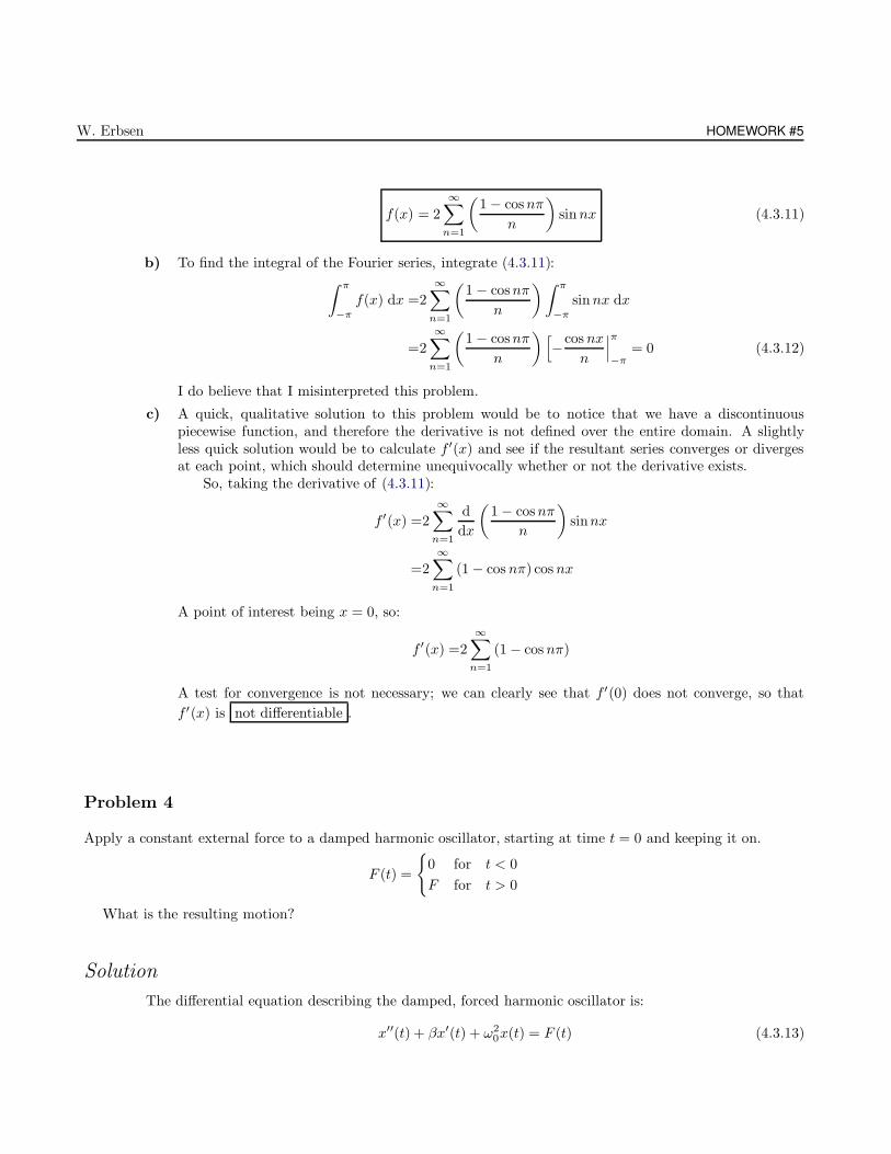
W. Erbsen HOMEWORK #5
f(x) = 2
∞∑
n=1
(1 − cosnπ
n
)sinnx (4.3.11)
b) To find the integral of the Fourier series, integrate (4.3.11):∫ π
−π
f(x) dx =2
∞∑
n=1
(1 − cosnπ
n
)∫ π
−π
sinnx dx
=2
∞∑
n=1
(1 − cosnπ
n
)[−cos nx
n
∣∣∣π
−π= 0 (4.3.12)
I do believe that I misinterpreted this problem.
c) A quick, qualitative solution to this problem would be to notice that we have a discontinuouspiecewise function, and therefore the derivative is not defined over the entire domain. A slightlyless quick solution would be to calculate f ′(x) and see if the resultant series converges or divergesat each point, which should determine unequivocally whether or not the derivative exists.
So, taking the derivative of (4.3.11):
f ′(x) =2
∞∑
n=1
d
dx
(1 − cosnπ
n
)sinnx
=2∞∑
n=1
(1 − cos nπ) cos nx
A point of interest being x = 0, so:
f ′(x) =2
∞∑
n=1
(1 − cos nπ)
A test for convergence is not necessary; we can clearly see that f ′(0) does not converge, so that
f ′(x) is not differentiable .
Problem 4
Apply a constant external force to a damped harmonic oscillator, starting at time t = 0 and keeping it on.
F (t) =
0 for t < 0
F for t > 0
What is the resulting motion?
Solution
The differential equation describing the damped, forced harmonic oscillator is:
x′′(t) + βx′(t) + ω20x(t) = F (t) (4.3.13)
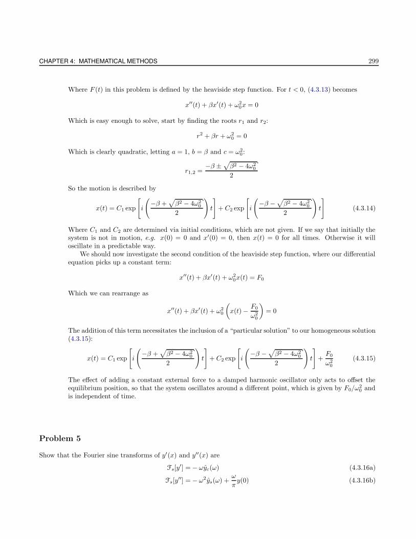
CHAPTER 4: MATHEMATICAL METHODS 299
Where F (t) in this problem is defined by the heaviside step function. For t < 0, (4.3.13) becomes
x′′(t) + βx′(t) + ω20x = 0
Which is easy enough to solve, start by finding the roots r1 and r2:
r2 + βr + ω20 = 0
Which is clearly quadratic, letting a = 1, b = β and c = ω20 :
r1,2 =−β ±
√β2 − 4ω2
0
2
So the motion is described by
x(t) = C1 exp
[i
(−β +
√β2 − 4ω2
0
2
)t
]+ C2 exp
[i
(−β −
√β2 − 4ω2
0
2
)t
](4.3.14)
Where C1 and C2 are determined via initial conditions, which are not given. If we say that initially thesystem is not in motion, e.g. x(0) = 0 and x′(0) = 0, then x(t) = 0 for all times. Otherwise it willoscillate in a predictable way.
We should now investigate the second condition of the heaviside step function, where our differentialequation picks up a constant term:
x′′(t) + βx′(t) + ω20x(t) = F0
Which we can rearrange as
x′′(t) + βx′(t) + ω20
(x(t) − F0
ω20
)= 0
The addition of this term necessitates the inclusion of a “particular solution” to our homogeneous solution(4.3.15):
x(t) = C1 exp
[i
(−β +
√β2 − 4ω2
0
2
)t
]+ C2 exp
[i
(−β −
√β2 − 4ω2
0
2
)t
]+F0
ω20
(4.3.15)
The effect of adding a constant external force to a damped harmonic oscillator only acts to offset theequilibrium position, so that the system oscillates around a different point, which is given by F0/ω
20 and
is independent of time.
Problem 5
Show that the Fourier sine transforms of y′(x) and y′′(x) are
Fs[y′] = − ωyc(ω) (4.3.16a)
Fs[y′′] = − ω2ys(ω) +
ω
πy(0) (4.3.16b)
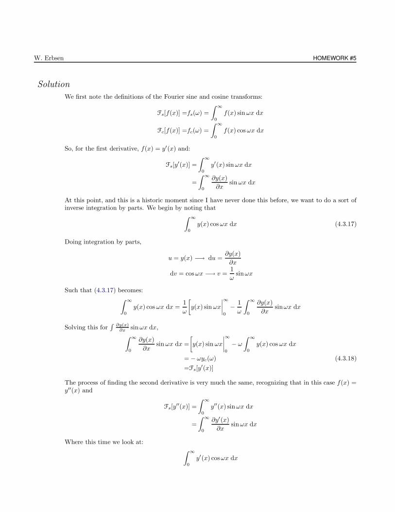
W. Erbsen HOMEWORK #5
Solution
We first note the definitions of the Fourier sine and cosine transforms:
Fs[f(x)] =fs(ω) =
∫ ∞
0
f(x) sinωx dx
Fc[f(x)] =fc(ω) =
∫ ∞
0
f(x) cosωx dx
So, for the first derivative, f(x) = y′(x) and:
Fs[y′(x)] =
∫ ∞
0
y′(x) sinωx dx
=
∫ ∞
0
∂y(x)
∂xsinωx dx
At this point, and this is a historic moment since I have never done this before, we want to do a sort ofinverse integration by parts. We begin by noting that
∫ ∞
0
y(x) cosωx dx (4.3.17)
Doing integration by parts,
u = y(x) −→ du =∂y(x)
∂x
dv = cosωx −→ v =1
ωsinωx
Such that (4.3.17) becomes:∫ ∞
0
y(x) cosωx dx =1
ω
[y(x) sin ωx
∣∣∣∣∞
0
− 1
ω
∫ ∞
0
∂y(x)
∂xsinωx dx
Solving this for∫ ∂y(x)
∂x sinωx dx,∫ ∞
0
∂y(x)
∂xsinωx dx =
[y(x) sin ωx
∣∣∣∣∞
0
− ω
∫ ∞
0
y(x) cosωx dx
= − ωyc(ω) (4.3.18)
=Fs[y′(x)]
The process of finding the second derivative is very much the same, recognizing that in this case f(x) =y′′(x) and
Fs[y′′(x)] =
∫ ∞
0
y′′(x) sinωx dx
=
∫ ∞
0
∂y′(x)
∂xsinωx dx
Where this time we look at:∫ ∞
0
y′(x) cosωx dx
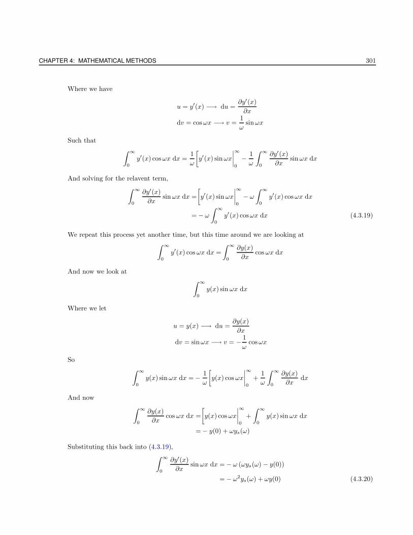
CHAPTER 4: MATHEMATICAL METHODS 301
Where we have
u = y′(x) −→ du =∂y′(x)
∂x
dv = cosωx −→ v =1
ωsinωx
Such that
∫ ∞
0
y′(x) cosωx dx =1
ω
[y′(x) sinωx
∣∣∣∣∞
0
− 1
ω
∫ ∞
0
∂y′(x)
∂xsinωx dx
And solving for the relavent term,
∫ ∞
0
∂y′(x)
∂xsinωx dx =
[y′(x) sinωx
∣∣∣∣∞
0
− ω
∫ ∞
0
y′(x) cosωx dx
= − ω
∫ ∞
0
y′(x) cosωx dx (4.3.19)
We repeat this process yet another time, but this time around we are looking at
∫ ∞
0
y′(x) cosωx dx =
∫ ∞
0
∂y(x)
∂xcosωx dx
And now we look at
∫ ∞
0
y(x) sin ωx dx
Where we let
u = y(x) −→ du =∂y(x)
∂x
dv = sinωx −→ v = − 1
ωcosωx
So
∫ ∞
0
y(x) sin ωx dx = − 1
ω
[y(x) cosωx
∣∣∣∣∞
0
+1
ω
∫ ∞
0
∂y(x)
∂xdx
And now
∫ ∞
0
∂y(x)
∂xcosωx dx =
[y(x) cosωx
∣∣∣∣∞
0
+
∫ ∞
0
y(x) sinωx dx
= − y(0) + ωys(ω)
Substituting this back into (4.3.19),∫ ∞
0
∂y′(x)
∂xsinωx dx = − ω (ωys(ω) − y(0))
= − ω2ys(ω) + ωy(0) (4.3.20)
W. Erbsen HOMEWORK #5
In summary, we have shown that:
Fs[y′] = −ωyc(ω)
Fs[y′′] = −ω2ys(ω) + ωy(0)
You might have noticed that what I found for Fs[y′′] differs from yours by a factor of 1/π in the last
term. I have no idea where that could have come from.
Problem 6
Show that the solution of
y′′ + 2µy′ + (β2 + µ2)y = g(x), µ > 0, β > 0, y(−∞) = y(∞) = 0 (4.3.21)
With g(±∞) = 0 is
y =1
β
∫ x
−∞g(ξ)e−µ(x−ξ) sin [β(x − ξ)] dξ (4.3.22)
Hint: Find Green’s function of the equation first.
Solution
As per the hint, I am going to go ahead and find Green’s function for (4.3.21). Substituting G(x− ξ) fory assuming that x > ξ, we solve the homogeneous analogue of our given differential equation:
G′′(x− ξ) + 2µG′(x− ξ) + (β2 + µ2)G(x− ξ) = 0
Finding the roots,
r2 + 2µr + (β2 + µ2) = 0
Letting a = 1, b = 2µ and c = β2 + µ2:
r1,2 =−2µ±
√4µ2 − 4(β2 + µ2)
2=µ± iβ
So that we have
G(x− ξ) =C1 cos[(µ+ iβ)(x − ξ)] + C2 sin[(µ− iβ)(x − ξ)]
=1
βsin[(µ− iβ)(x − ξ)] (4.3.23)
Due to the boundary conditions of the problem. At this point we should note that this problem representsa driven, damped harmonic oscillator, whose solution was discussed in an earlier problem. The solution
CHAPTER 4: MATHEMATICAL METHODS 303
to this type of problem using Green’s function is given in M&W in the prompt of problem 9-7. Tailoringit to our case,
y(x) =
∫ x
−∞G(x− ξ)g(ξ) dξ (4.3.24)
The finite upper limit comes from the fact that x in this problem really should be t, and up to this pointwe have been assuming that for x− ξ ≤ 0, G(x− ξ) = 0. To make this more transparent, we note thatfor a harmonic oscillator, we would have likely chosen “x” to be “t,” and “ξ” to be “t′.” In this case oursolution for y(x) (or y(t), rather) is represented by an integral over past times t.
Substituting (4.3.23) into (4.3.24),
y(x) =1
β
∫ x
−∞sin[(µ− iβ)x]g(ξ) dξ (4.3.25)
Where we can say
sin[(µ− iβ)x] =1
2iexp[(µ− iβ)(x − ξ)] − exp[(−µ+ iβ)(x − ξ)]
=1
2iexp[µx− µξ − iβx + iβξ] − exp[−µx+ µξ + iβx − iβξ]
=1
2iexp[µ(x− ξ) + iβ(x − ξ)] − exp[−µ(x− ξ) + iβ(x − ξ)]
=exp[µ(x− ξ)]
2iexp[iβ(x − ξ)] − exp[−iβ(x − ξ)]
=exp[µ(x− ξ)] sin [β(x − ξ)] (4.3.26)
Now substituting (4.3.26) back into (4.3.25):
y(x) =1
β
∫ x
−∞exp[µ(x− ξ)] sin [β(x− ξ)] g(ξ) dξ
In case you couldn’t tell I worked backwards a bit, sorry for the missteps in logic. I am very ignorant toGreen’s functions (I find the entire thing very confusing), however it is an invaluable mathematical tool,one I hope to master soon.
4.4 Homework #6
Problem 1
Find the Laplace transform of f(t) = tet, and determine the region of existence.
Solution
W. Erbsen HOMEWORK #6
We know that the Laplace Transform of some function f(t) is given by
L f(t) = F (s) =
∫ ∞
0
f(t)e−st dt
And in our case,
L f(t) =
∫ ∞
0
tete−st dt
=
∫ ∞
0
te−(s−1)t dt
u = t, du = 1dv = e−(s−1)t, v = − 1
s−1e−(s−1)t
=
[− t
s− 1e−(s−1)t
∣∣∣∣∞
0
+1
s− 1
∫ ∞
0
e−(s−1)t dt
=
[− 1
(s− 1)2e−(s−1)t
∣∣∣∣∞
0
=1
(s− 1)2
We can see that in the last limit, the result will be convergent only if s− 1 < 0, or s > 1, so
F (s) =1
(s− 1)2for s > 1
Problem 2
Find the inverse Laplace Transform of
a)1
s3 − s2(4.4.1a)
b)s2 + s− 1
s3 − 2s2 + s− 2(4.4.1b)
Solution
a) As per the hint, let’s go ahead and employ partial fractions on (4.4.1a):
1
s3 − s2=⇒ 1
s2(s− 1)=A
s2+B
s+
C
s− 1
1 =A(s− 1) + Bs(s − 1) + Cs2
Let s = 0: 1 = −A −→ A = −1
Let s = 1: 1 =Cs2 −→ C = 1
Let A = −1, C = 1: 1 =1 − s+Bs(s − 1) + s2 −→ B = 1
So, (4.4.1a) becomes
CHAPTER 4: MATHEMATICAL METHODS 305
1
s3 − s2=
1
s− 1− 1
s2− 1
s(4.4.2)
Where we note that
Let
=
∫ ∞
0
et · e−st dt =
∫ ∞
0
e−(s−1)t dt =1
s− 1(4.4.3a)
L t =
∫ ∞
0
te−st dt =1
s
∫ ∞
0
e−st dt =1
s2(4.4.3b)
L 1 =
∫ ∞
0
e−st dt =1
s(4.4.3c)
Substituting (4.4.3a)-(4.4.3c) into (4.4.2),
1
s3 − s2= et − t − 1
b) This time we only need to factor; no partial fractions is needed:
s2 + s− 1
s3 − 2s2 + s− 2=
(s2 + 1)
(s2 + 1)(s− 2)+
(s2 + 1) + (s− 2)
(s2 + 1)(s− 2)=
1
s2 + 1+
1
s− 2(4.4.4)
We note the Laplace Transforms of the following functions
L sin t =
∫ ∞
0
sin te−st dt
=1
2i
∫ ∞
0
[eit − e−it
]e−st dt
=1
2i
∫ ∞
0
[e(i−s)t − e−(i+s)t
]dt
=1
2i
[−e
(i−s)t
s− i− e−(i+s)t
s+ i
∣∣∣∣∞
0
=1
2i
[1
s− i− 1
s+ i
]
=1
2i
[2i
s2 + 1
]
=1
s2 + 1(4.4.5)
Le2t
=
∫ ∞
0
e2t · e−st dt =
∫ ∞
0
e−(s−2)t dt =1
s− 2(4.4.6)
Putting (4.4.5) and (4.4.6) into (4.4.4),
s2 + s− 1
s3 − 2s2 + s− 2= sin t + e2t
Problem 3
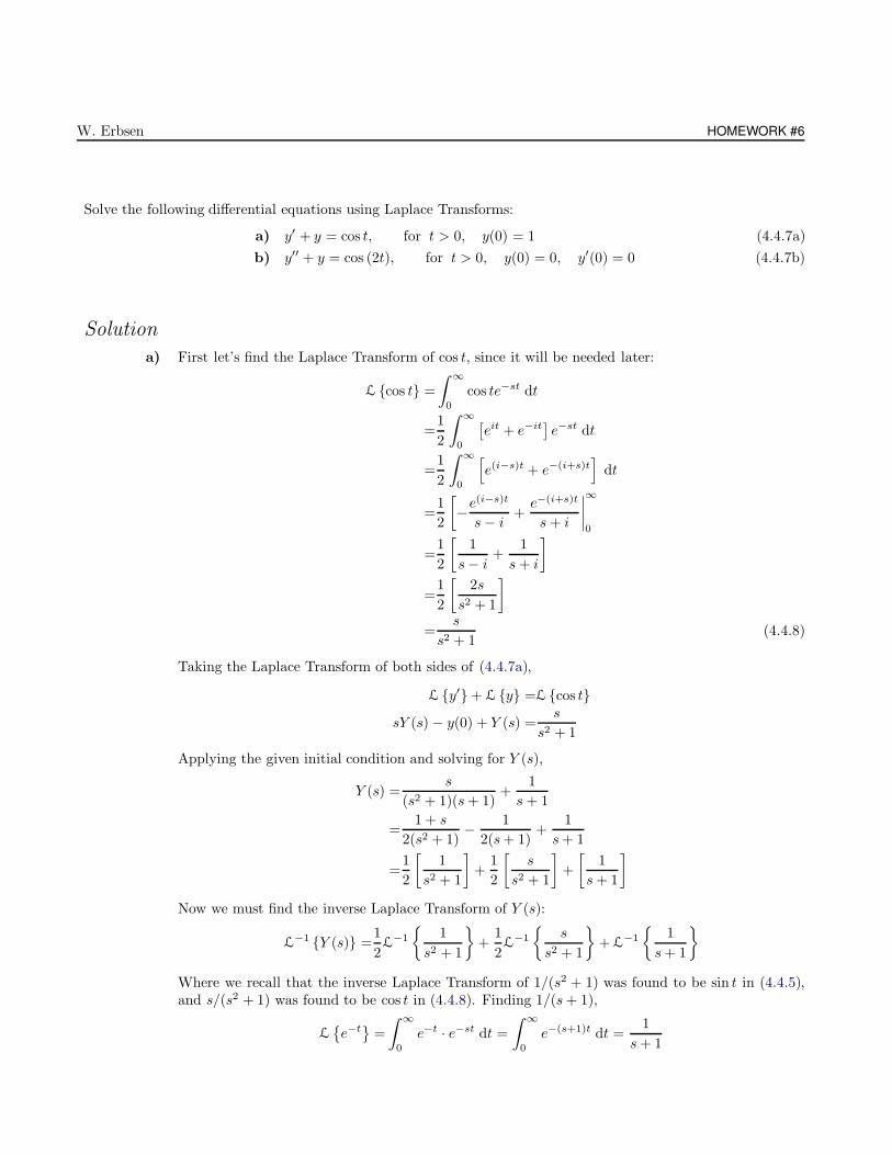
W. Erbsen HOMEWORK #6
Solve the following differential equations using Laplace Transforms:
a) y′ + y = cos t, for t > 0, y(0) = 1 (4.4.7a)
b) y′′ + y = cos (2t), for t > 0, y(0) = 0, y′(0) = 0 (4.4.7b)
Solution
a) First let’s find the Laplace Transform of cos t, since it will be needed later:
L cos t =
∫ ∞
0
cos te−st dt
=1
2
∫ ∞
0
[eit + e−it
]e−st dt
=1
2
∫ ∞
0
[e(i−s)t + e−(i+s)t
]dt
=1
2
[−e
(i−s)t
s− i+e−(i+s)t
s+ i
∣∣∣∣∞
0
=1
2
[1
s− i+
1
s+ i
]
=1
2
[2s
s2 + 1
]
=s
s2 + 1(4.4.8)
Taking the Laplace Transform of both sides of (4.4.7a),
L y′ + L y =L cos t
sY (s) − y(0) + Y (s) =s
s2 + 1
Applying the given initial condition and solving for Y (s),
Y (s) =s
(s2 + 1)(s+ 1)+
1
s+ 1
=1 + s
2(s2 + 1)− 1
2(s+ 1)+
1
s+ 1
=1
2
[1
s2 + 1
]+
1
2
[s
s2 + 1
]+
[1
s+ 1
]
Now we must find the inverse Laplace Transform of Y (s):
L−1 Y (s) =
1
2L
−1
1
s2 + 1
+
1
2L
−1
s
s2 + 1
+ L
−1
1
s+ 1
Where we recall that the inverse Laplace Transform of 1/(s2 + 1) was found to be sin t in (4.4.5),and s/(s2 + 1) was found to be cos t in (4.4.8). Finding 1/(s+ 1),
Le−t
=
∫ ∞
0
e−t · e−st dt =
∫ ∞
0
e−(s+1)t dt =1
s+ 1
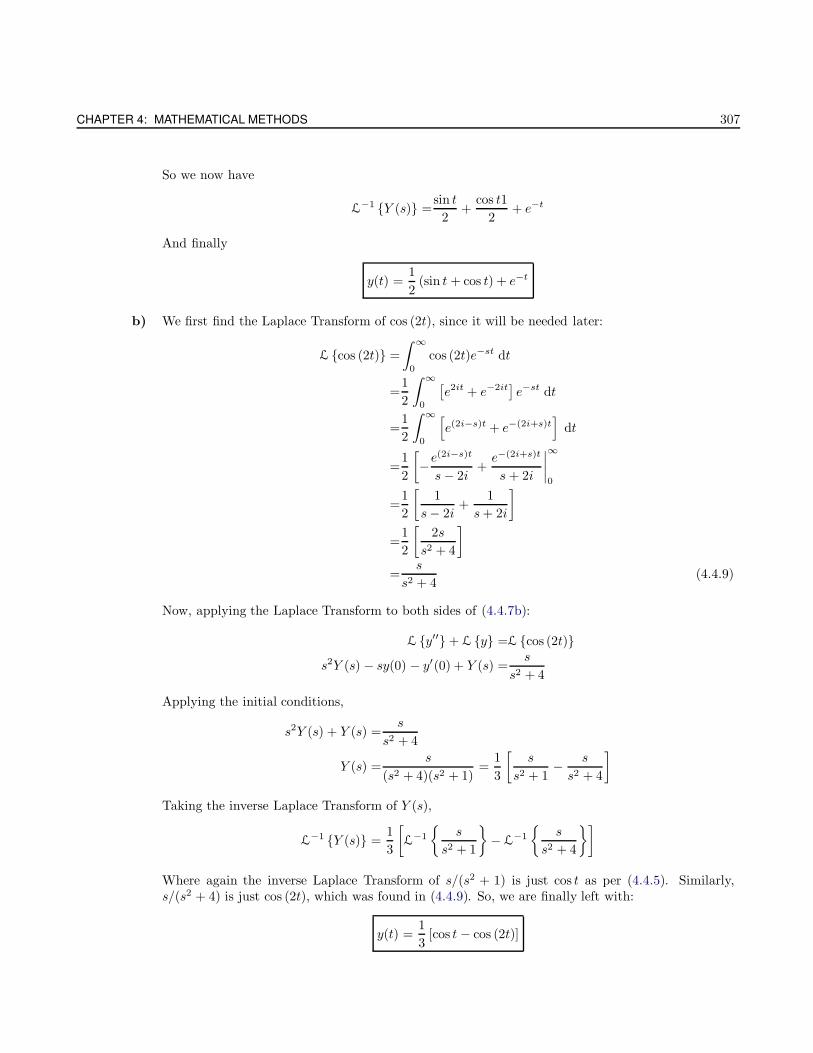
CHAPTER 4: MATHEMATICAL METHODS 307
So we now have
L−1 Y (s) =
sin t
2+
cos t1
2+ e−t
And finally
y(t) =1
2(sin t + cos t) + e−t
b) We first find the Laplace Transform of cos (2t), since it will be needed later:
L cos (2t) =
∫ ∞
0
cos (2t)e−st dt
=1
2
∫ ∞
0
[e2it + e−2it
]e−st dt
=1
2
∫ ∞
0
[e(2i−s)t + e−(2i+s)t
]dt
=1
2
[−e
(2i−s)t
s− 2i+e−(2i+s)t
s+ 2i
∣∣∣∣∞
0
=1
2
[1
s− 2i+
1
s+ 2i
]
=1
2
[2s
s2 + 4
]
=s
s2 + 4(4.4.9)
Now, applying the Laplace Transform to both sides of (4.4.7b):
L y′′ + L y =L cos (2t)s2Y (s) − sy(0) − y′(0) + Y (s) =
s
s2 + 4
Applying the initial conditions,
s2Y (s) + Y (s) =s
s2 + 4
Y (s) =s
(s2 + 4)(s2 + 1)=
1
3
[s
s2 + 1− s
s2 + 4
]
Taking the inverse Laplace Transform of Y (s),
L−1 Y (s) =
1
3
[L
−1
s
s2 + 1
− L
−1
s
s2 + 4
]
Where again the inverse Laplace Transform of s/(s2 + 1) is just cos t as per (4.4.5). Similarly,s/(s2 + 4) is just cos (2t), which was found in (4.4.9). So, we are finally left with:
y(t) =1
3[cos t − cos (2t)]
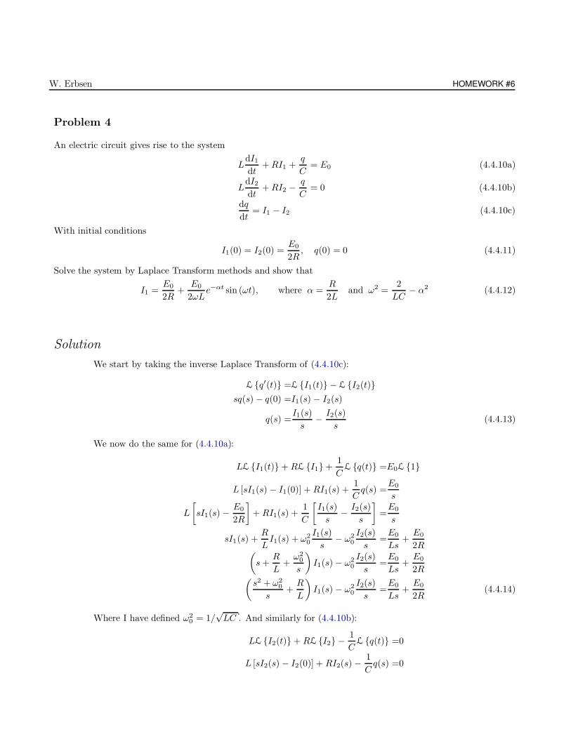
W. Erbsen HOMEWORK #6
Problem 4
An electric circuit gives rise to the system
LdI1dt
+RI1 +q
C= E0 (4.4.10a)
LdI2dt
+RI2 −q
C= 0 (4.4.10b)
dq
dt= I1 − I2 (4.4.10c)
With initial conditions
I1(0) = I2(0) =E0
2R, q(0) = 0 (4.4.11)
Solve the system by Laplace Transform methods and show that
I1 =E0
2R+
E0
2ωLe−αt sin (ωt), where α =
R
2Land ω2 =
2
LC− α2 (4.4.12)
Solution
We start by taking the inverse Laplace Transform of (4.4.10c):
L q′(t) =L I1(t) − L I2(t)sq(s) − q(0) =I1(s) − I2(s)
q(s) =I1(s)
s− I2(s)
s(4.4.13)
We now do the same for (4.4.10a):
LL I1(t) + RL I1 +1
CL q(t) =E0L 1
L [sI1(s) − I1(0)] + RI1(s) +1
Cq(s) =
E0
s
L
[sI1(s) −
E0
2R
]+ RI1(s) +
1
C
[I1(s)
s− I2(s)
s
]=E0
s
sI1(s) +R
LI1(s) + ω2
0
I1(s)
s− ω2
0
I2(s)
s=E0
Ls+E0
2R(s+
R
L+ω2
0
s
)I1(s) − ω2
0
I2(s)
s=E0
Ls+E0
2R(s2 + ω2
0
s+R
L
)I1(s) − ω2
0
I2(s)
s=E0
Ls+E0
2R(4.4.14)
Where I have defined ω20 = 1/
√LC . And similarly for (4.4.10b):
LL I2(t) + RL I2 −1
CL q(t) =0
L [sI2(s) − I2(0)] + RI2(s) −1
Cq(s) =0
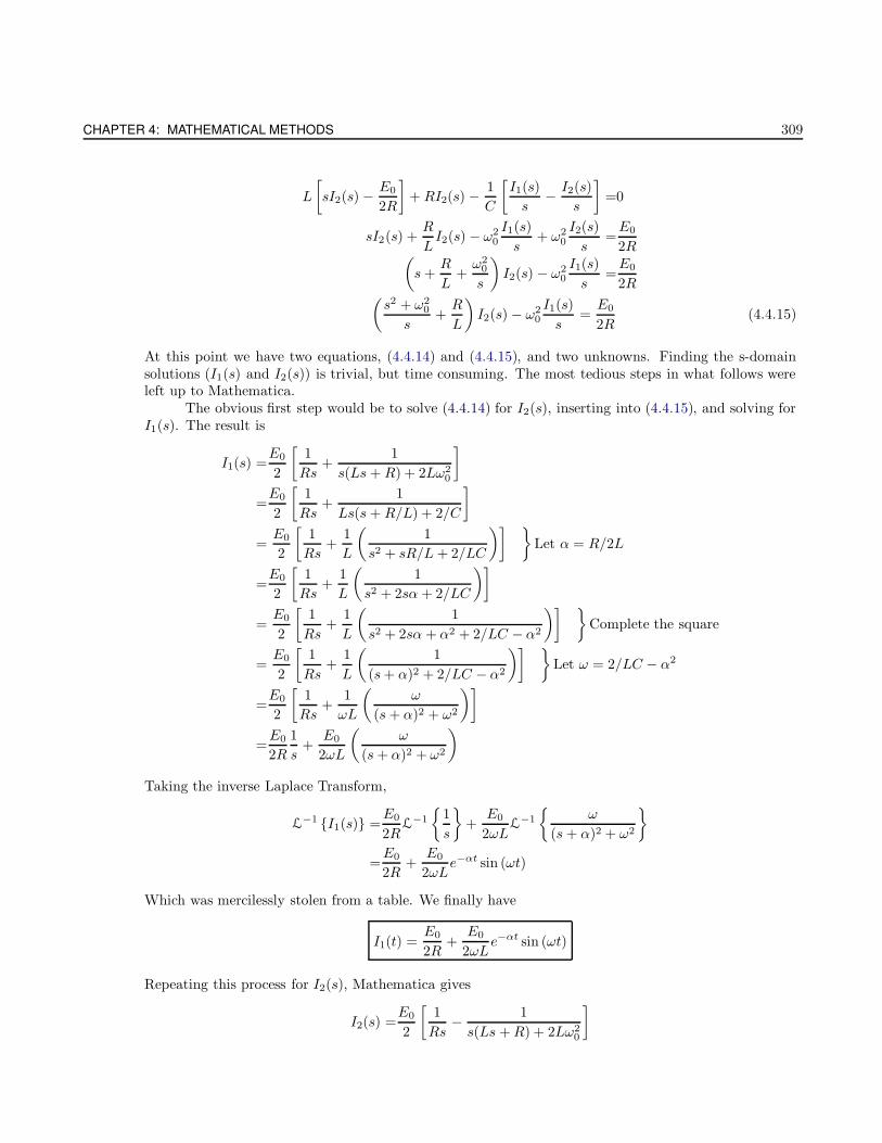
CHAPTER 4: MATHEMATICAL METHODS 309
L
[sI2(s) −
E0
2R
]+ RI2(s) −
1
C
[I1(s)
s− I2(s)
s
]=0
sI2(s) +R
LI2(s) − ω2
0
I1(s)
s+ ω2
0
I2(s)
s=E0
2R(s+
R
L+ω2
0
s
)I2(s) − ω2
0
I1(s)
s=E0
2R(s2 + ω2
0
s+R
L
)I2(s) − ω2
0
I1(s)
s=E0
2R(4.4.15)
At this point we have two equations, (4.4.14) and (4.4.15), and two unknowns. Finding the s-domainsolutions (I1(s) and I2(s)) is trivial, but time consuming. The most tedious steps in what follows wereleft up to Mathematica.
The obvious first step would be to solve (4.4.14) for I2(s), inserting into (4.4.15), and solving forI1(s). The result is
I1(s) =E0
2
[1
Rs+
1
s(Ls+ R) + 2Lω20
]
=E0
2
[1
Rs+
1
Ls(s+ R/L) + 2/C
]
=E0
2
[1
Rs+
1
L
(1
s2 + sR/L + 2/LC
)] Let α = R/2L
=E0
2
[1
Rs+
1
L
(1
s2 + 2sα + 2/LC
)]
=E0
2
[1
Rs+
1
L
(1
s2 + 2sα + α2 + 2/LC − α2
)] Complete the square
=E0
2
[1
Rs+
1
L
(1
(s+ α)2 + 2/LC − α2
)] Let ω = 2/LC − α2
=E0
2
[1
Rs+
1
ωL
(ω
(s+ α)2 + ω2
)]
=E0
2R
1
s+
E0
2ωL
(ω
(s+ α)2 + ω2
)
Taking the inverse Laplace Transform,
L−1 I1(s) =
E0
2RL
−1
1
s
+
E0
2ωLL
−1
ω
(s+ α)2 + ω2
=E0
2R+
E0
2ωLe−αt sin (ωt)
Which was mercilessly stolen from a table. We finally have
I1(t) =E0
2R+
E0
2ωLe−αt sin (ωt)
Repeating this process for I2(s), Mathematica gives
I2(s) =E0
2
[1
Rs− 1
s(Ls +R) + 2Lω20
]
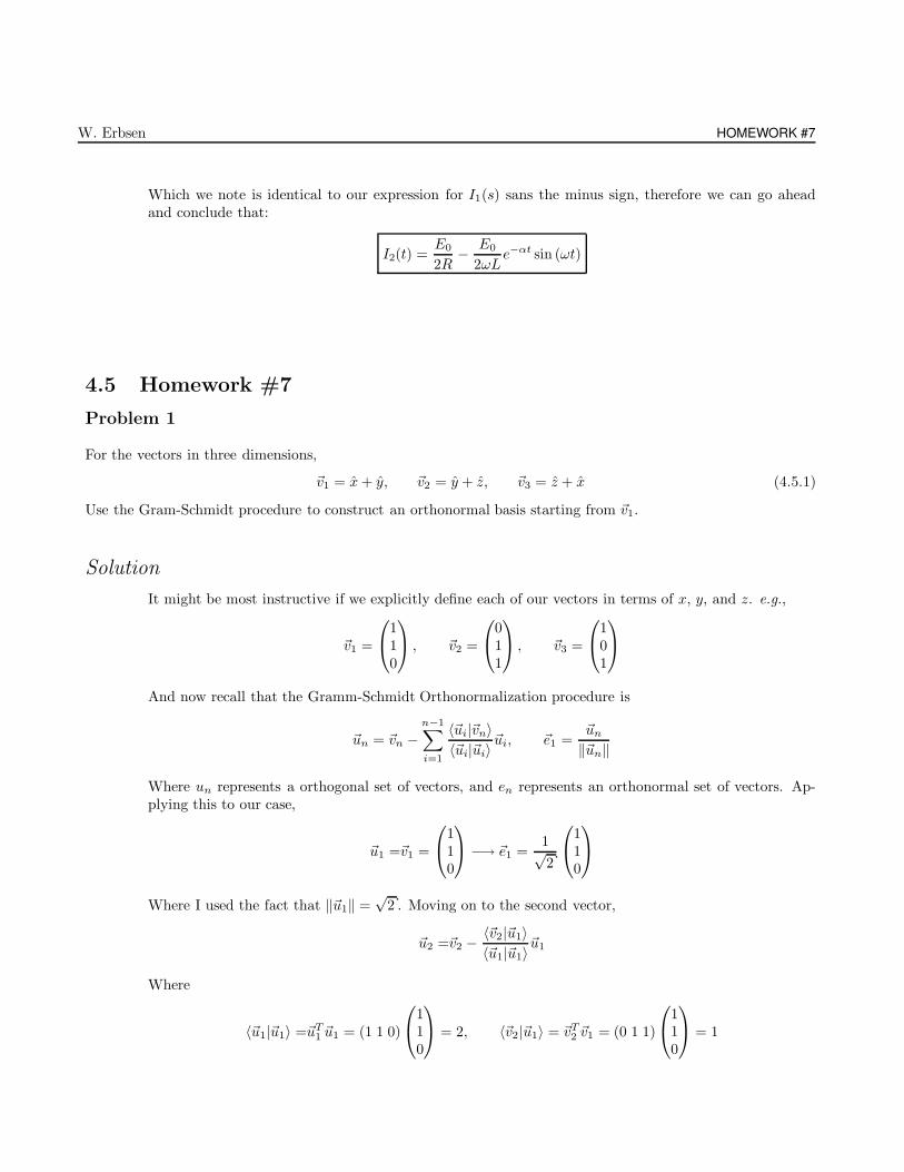
W. Erbsen HOMEWORK #7
Which we note is identical to our expression for I1(s) sans the minus sign, therefore we can go aheadand conclude that:
I2(t) =E0
2R− E0
2ωLe−αt sin (ωt)
4.5 Homework #7
Problem 1
For the vectors in three dimensions,
~v1 = x+ y, ~v2 = y + z, ~v3 = z + x (4.5.1)
Use the Gram-Schmidt procedure to construct an orthonormal basis starting from ~v1.
Solution
It might be most instructive if we explicitly define each of our vectors in terms of x, y, and z. e.g.,
~v1 =
110
, ~v2 =
011
, ~v3 =
101
And now recall that the Gramm-Schmidt Orthonormalization procedure is
~un = ~vn −n−1∑
i=1
〈~ui|~vn〉〈~ui|~ui〉
~ui, ~e1 =~un
‖~un‖
Where un represents a orthogonal set of vectors, and en represents an orthonormal set of vectors. Ap-plying this to our case,
~u1 =~v1 =
110
−→ ~e1 =
1√2
110
Where I used the fact that ‖~u1‖ =√
2 . Moving on to the second vector,
~u2 =~v2 −〈~v2|~u1〉〈~u1|~u1〉
~u1
Where
〈~u1|~u1〉 =~uT1 ~u1 = (1 1 0)
110
= 2, 〈~v2|~u1〉 = ~vT
2 ~v1 = (0 1 1)
110
= 1
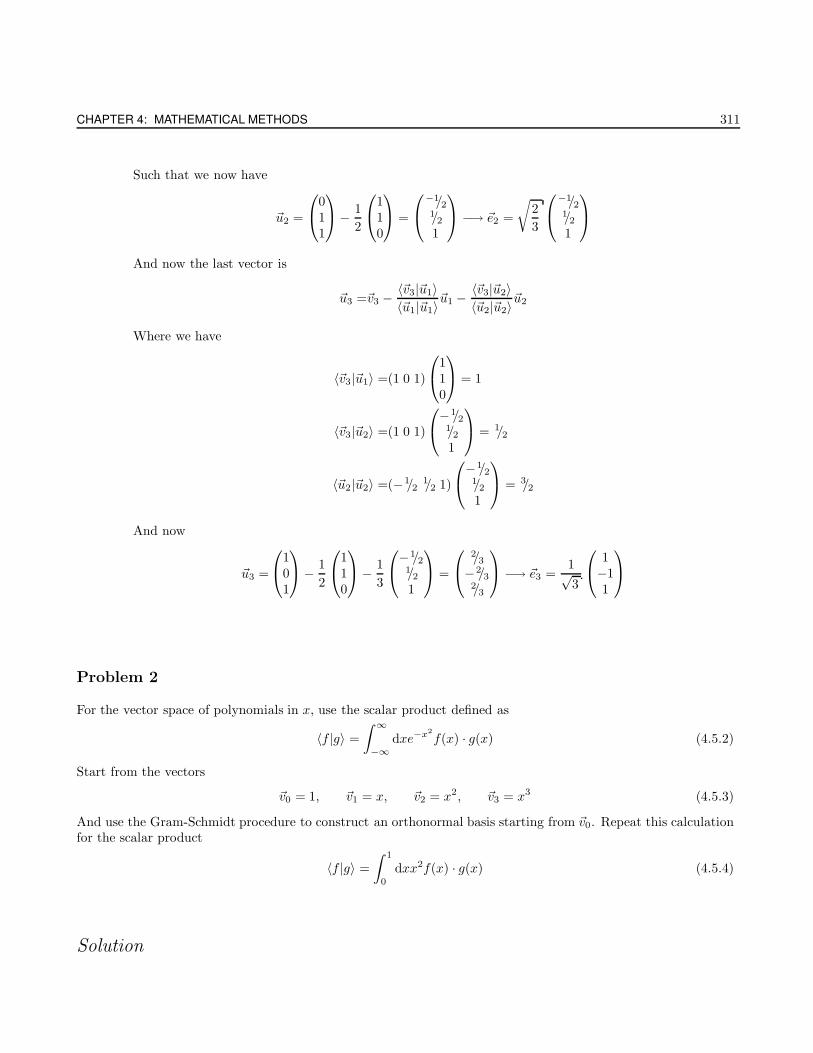
CHAPTER 4: MATHEMATICAL METHODS 311
Such that we now have
~u2 =
011
− 1
2
110
=
−1/21/21
−→ ~e2 =
√2
3
−1/21/21
And now the last vector is
~u3 =~v3 −〈~v3|~u1〉〈~u1|~u1〉
~u1 −〈~v3|~u2〉〈~u2|~u2〉
~u2
Where we have
〈~v3|~u1〉 =(1 0 1)
110
= 1
〈~v3|~u2〉 =(1 0 1)
−1/21/21
= 1/2
〈~u2|~u2〉 =(−1/21/2 1)
−1/21/21
= 3/2
And now
~u3 =
101
− 1
2
110
− 1
3
−1/21/21
=
2/3−2/32/3
−→ ~e3 =
1√3
1−11
Problem 2
For the vector space of polynomials in x, use the scalar product defined as
〈f |g〉 =
∫ ∞
−∞dxe−x2
f(x) · g(x) (4.5.2)
Start from the vectors
~v0 = 1, ~v1 = x, ~v2 = x2, ~v3 = x3 (4.5.3)
And use the Gram-Schmidt procedure to construct an orthonormal basis starting from ~v0. Repeat this calculationfor the scalar product
〈f |g〉 =
∫ 1
0
dxx2f(x) · g(x) (4.5.4)
Solution
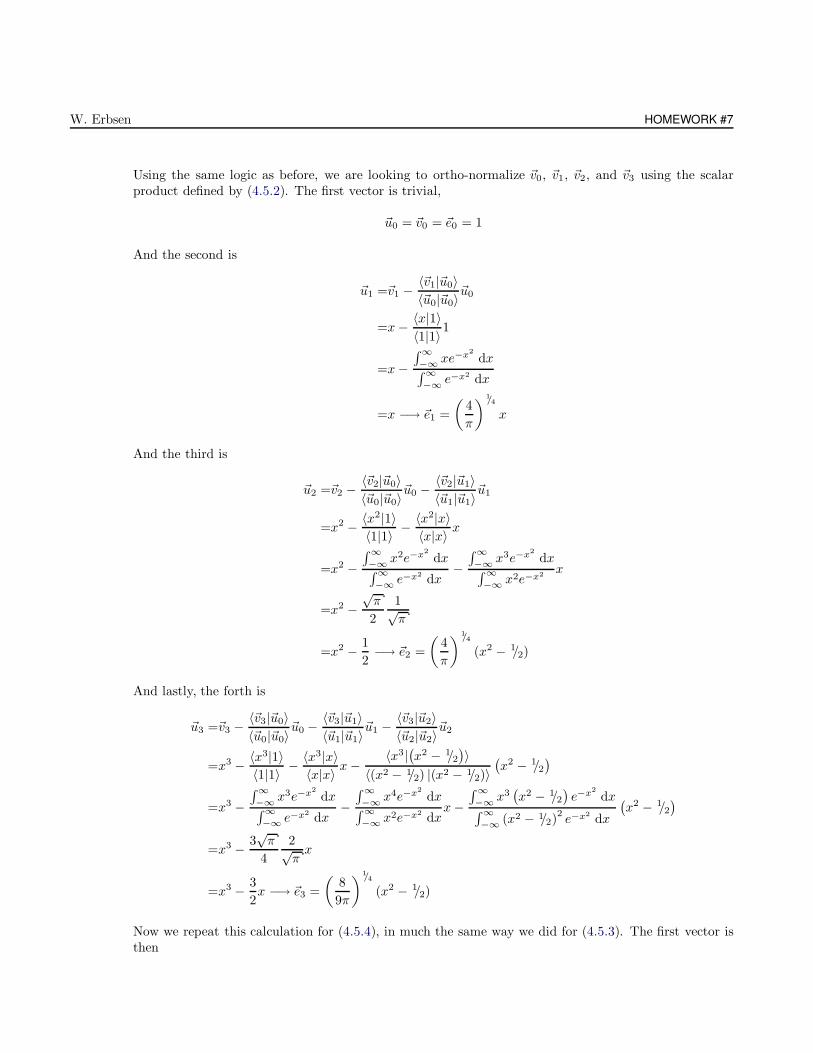
W. Erbsen HOMEWORK #7
Using the same logic as before, we are looking to ortho-normalize ~v0, ~v1, ~v2, and ~v3 using the scalarproduct defined by (4.5.2). The first vector is trivial,
~u0 = ~v0 = ~e0 = 1
And the second is
~u1 =~v1 −〈~v1|~u0〉〈~u0|~u0〉
~u0
=x− 〈x|1〉〈1|1〉1
=x−∫∞−∞ xe−x2
dx∫∞−∞ e−x2 dx
=x −→ ~e1 =
(4
π
) 1/4
x
And the third is
~u2 =~v2 −〈~v2|~u0〉〈~u0|~u0〉
~u0 −〈~v2|~u1〉〈~u1|~u1〉
~u1
=x2 − 〈x2|1〉〈1|1〉 − 〈x2|x〉
〈x|x〉 x
=x2 −∫∞−∞ x2e−x2
dx∫∞−∞ e−x2
dx−∫∞−∞ x3e−x2
dx∫∞−∞ x2e−x2
x
=x2 −√π
2
1√π
=x2 − 1
2−→ ~e2 =
(4
π
) 1/4
(x2 − 1/2)
And lastly, the forth is
~u3 =~v3 −〈~v3|~u0〉〈~u0|~u0〉
~u0 −〈~v3|~u1〉〈~u1|~u1〉
~u1 −〈~v3|~u2〉〈~u2|~u2〉
~u2
=x3 − 〈x3|1〉〈1|1〉 − 〈x3|x〉
〈x|x〉 x− 〈x3|(x2 − 1/2
)〉
〈(x2 − 1/2) |(x2 − 1/2)〉(x2 − 1/2
)
=x3 −∫∞−∞ x3e−x2
dx∫∞−∞ e−x2
dx−∫∞−∞ x4e−x2
dx∫∞−∞ x2e−x2
dxx−
∫∞−∞ x3
(x2 − 1/2
)e−x2
dx∫∞−∞ (x2 − 1/2)
2e−x2
dx
(x2 − 1/2
)
=x3 − 3√π
4
2√πx
=x3 − 3
2x −→ ~e3 =
(8
9π
)1/4
(x2 − 1/2)
Now we repeat this calculation for (4.5.4), in much the same way we did for (4.5.3). The first vector isthen
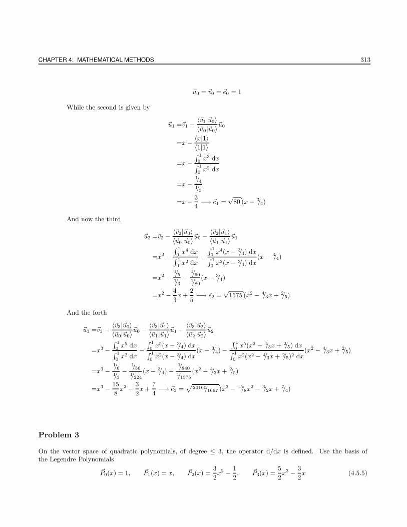
CHAPTER 4: MATHEMATICAL METHODS 313
~u0 = ~v0 = ~e0 = 1
While the second is given by
~u1 =~v1 −〈~v1|~u0〉〈~u0|~u0〉
~u0
=x− 〈x|1〉〈1|1〉
=x−∫ 1
0x3 dx
∫ 1
0x2 dx
=x−1/41/3
=x− 3
4−→ ~e1 =
√80 (x− 3/4)
And now the third
~u2 =~v2 −〈~v2|~u0〉〈~u0|~u0〉
~u0 −〈~v2|~u1〉〈~u1|~u1〉
~u1
=x2 −∫ 1
0x4 dx
∫ 1
0 x2 dx
−∫ 1
0x4(x− 3/4) dx
∫ 1
0 x2(x− 3/4) dx
(x− 3/4)
=x2 −1/51/3
−1/60
1/80(x− 3/4)
=x2 − 4
3x+
2
5−→ ~e2 =
√1575 (x2 − 4/3x+ 2/5)
And the forth
~u3 =~v3 −〈~v3|~u0〉〈~u0|~u0〉
~u0 −〈~v3|~u1〉〈~u1|~u1〉
~u1 −〈~v3|~u2〉〈~u2|~u2〉
~u2
=x3 −∫ 1
0x5 dx
∫ 1
0x2 dx
−∫ 1
0x5(x− 3/4) dx
∫ 1
0x2(x− 3/4) dx
(x− 3/4) −∫ 1
0x5(x2 − 4/3x+ 2/5) dx
∫ 1
0x2(x2 − 4/3x+ 2/5)2 dx
(x2 − 4/3x+ 2/5)
=x3 −1/61/3
−1/56
1/224(x− 3/4) −
1/840
1/1575(x2 − 4/3x+ 2/5)
=x3 − 15
8x2 − 3
2x+
7
4−→ ~e3 =
√20160/1667 (x3 − 15/8x
2 − 3/2x+ 7/4)
Problem 3
On the vector space of quadratic polynomials, of degree ≤ 3, the operator d/dx is defined. Use the basis ofthe Legendre Polynomials
~P0(x) = 1, ~P1(x) = x, ~P2(x) =3
2x2 − 1
2, ~P3(x) =
5
2x3 − 3
2x (4.5.5)
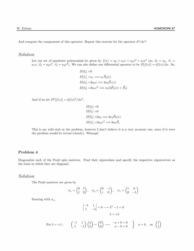
W. Erbsen HOMEWORK #7
And compute the components of this operator. Repeat this exercise for the operator d2/dx2.
Solution
Let our set of quadratic polynomials be given by f(x) = a0 + a1x + a2x2 + a3x
3 (so, ~v0 = a0, ~v1 =a1x, ~v2 = a2x
2, ~v3 = a3x3). We can also define our differential operator to be D[f(x)] = df(x)/dx. So,
D[~v0] =0
D[~v1] =a1 =⇒ a1~P0(x)
D[~v2] =2a2x =⇒ 2a2~P1(x)
D[~v3] =3a3x2 =⇒ a3(2 ~P2(x) + ~P0)
And if we let D2 [f(x)] = df(x)2/dx2,
D[~v0] =0
D[~v1] =0
D[~v2] =2a2 =⇒ 2a2~P0(x)
D[~v3] =3a3x2 =⇒ 6a3
~P1
This is my wild stab at the problem, however I don’t believe it is a very accurate one, since if it werethe problem would be trivial (clearly). Whoops!
Problem 4
Diagonalize each of the Pauli spin matrices. Find their eigenvalues and specify the respective eigenvectors asthe basis in which they are diagonal.
Solution
The Pauli matrices are given by
σx =
(0 11 0
), σy =
(0 −ii 0
), σz =
(1 00 −1
)
Starting with σx,∣∣∣∣−λ 11 −λ
∣∣∣∣ = 0 −→ λ2 − 1 = 0
λ = ±1
For λ = +1 :
(−1 11 −1
)(ab
)=
(00
)−→ −a+ b = 0
a− b = 0
a = b, so
(11
)
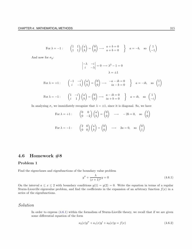
CHAPTER 4: MATHEMATICAL METHODS 315
For λ = −1 :
(1 11 1
)(ab
)=
(00
)−→ a+ b = 0
a+ b = 0
a = −b, so
(1−1
)
And now for σy:∣∣∣∣−λ −ii −λ
∣∣∣∣ = 0 −→ λ2 − 1 = 0
λ = ±1
For λ = +1 :
(−1 −ii −1
)(ab
)=
(00
)−→ −a − ib = 0
ia − b = 0
a = −ib, so
(1i
)
For λ = −1 :
(1 −ii 1
)(ab
)=
(00
)−→ a− ib = 0
ia + b = 0
a = ib, so
(1−i
)
In analyzing σz we immidiately recognize that λ = ±1, since it is diagonal. So, we have
For λ = +1 :
(0 00 −2
)(ab
)=
(00
)−→ − 2b = 0, so
(10
)
For λ = −1 :
(2 00 0
)(ab
)=
(00
)−→ 2a = 0, so
(01
)
4.6 Homework #8
Problem 1
Find the eigenvlaues and eigenfunctions of the boundary value problem
y′′ +λ
(x+ 1)2y = 0 (4.6.1)
On the interval a ≤ x ≤ 2 with boundary conditions y(1) = y(2) = 0. Write the equation in terms of a regularSturm-Liouville eigenvalue problem, and find the coefficients in the expansion of an arbitrary function f(x) in aseries of the eigenfunctions.
Solution
In order to express (4.6.1) within the formalism of Sturm-Lioville theory, we recall that if we are givensome differential equation of the form
a2(x)y′′ + a1(x)y
′ + a0(x)y = f(x) (4.6.2)
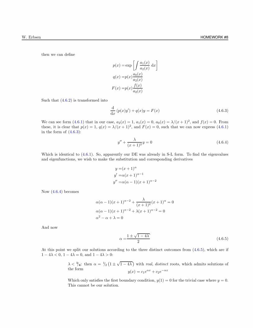
W. Erbsen HOMEWORK #8
then we can define
p(x) = exp
[∫a1(x)
a2(x)dx
]
q(x) =p(x)a0(x)
a2(x)
F (x) =p(x)f(x)
a2(x)
Such that (4.6.2) is transformed into
d
dx(p(x)y′) + q(x)y = F (x) (4.6.3)
We can see form (4.6.1) that in our case, a2(x) = 1, a1(x) = 0, a0(x) = λ/(x+ 1)2, and f(x) = 0. Fromthese, it is clear that p(x) = 1, q(x) = λ/(x+ 1)2, and F (x) = 0, such that we can now express (4.6.1)in the form of (4.6.3):
y′′ +λ
(x + 1)2y = 0 (4.6.4)
Which is identical to (4.6.1). So, apparently our DE was already in S-L form. To find the eigenvaluesand eigenfunctions, we wish to make the substitution and corresponding derivatives
y =(x+ 1)α
y′ =α(x+ 1)α−1
y′′ =α(α− 1)(x+ 1)α−2
Now (4.6.4) becomes
α(α− 1)(x+ 1)α−2 +λ
(x+ 1)2(x+ 1)α = 0
α(α− 1)(x+ 1)α−2 + λ(x+ 1)α−2 = 0
α2 − α+ λ = 0
And now
α =1 ±
√1 − 4λ
2(4.6.5)
At this point we split our solutions according to the three distinct outcomes from (4.6.5), which are if1 − 4λ < 0, 1 − 4λ = 0, and 1 − 4λ > 0:
λ < 1/4: then α = 1/2(1 ±
√1 − 4λ
)with real, distinct roots, which admits solutions of
the formy(x) = c1e
αx + c2e−αx
Which only satisfies the first boundary condition, y(1) = 0 for the trivial case where y = 0.This cannot be our solution.
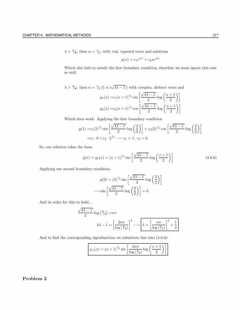
CHAPTER 4: MATHEMATICAL METHODS 317
λ = 1/4: then α = 1/2, with real, repeated roots and solutions
y(x) = c1eαx + c2xe
αx
Which also fails to satisfy the first boundary condition, therefore we must ignore this caseas well.
λ > 1/4: then α = 1/2(1 ± i
√4λ− 1
)with complex, distinct roots and
y1(x) =c1(x+ 1)1/2 sin
[√4λ − 1
2log
(x+ 1
2
)]
y2(x) =c2(x+ 1)1/2 cos
[√4λ− 1
2log
(x+ 1
2
)]
Which does work. Applying the first boundary condition
y(1) =c1(2)1/2 sin
[√4λ− 1
2log
(2
2
)]+ c2(2)
1/2 cos
[√4λ − 1
2log
(2
2
)]
=c1 · 0 + c2 · 21/2 −→ c1 = 1, c2 = 0
So, our solution takes the form
y(x) = y1(x) = (x+ 1)1/2 sin
[√4λ− 1
2log
(x+ 1
2
)](4.6.6)
Applying our second boundary condition,
y(2) = (3)1/2 sin
[√4λ− 1
2log
(3
2
)]
−→ sin
[√4λ − 1
2log
(3
2
)]= 0
And in order for this to hold...
√4λ− 1
2log(
3/2)
=nπ
4λ− 1 =
[2nπ
log (3/2)
]2−→ λ =
[nπ
log (3/2)
]2+
1
4
And to find the corresponding eigenfunction we substitute this into (4.6.6):
ϕn(x) = (x+ 1)1/2 sin
[2nπ
log (3/2)log
(x+ 1
2
)]
Problem 2
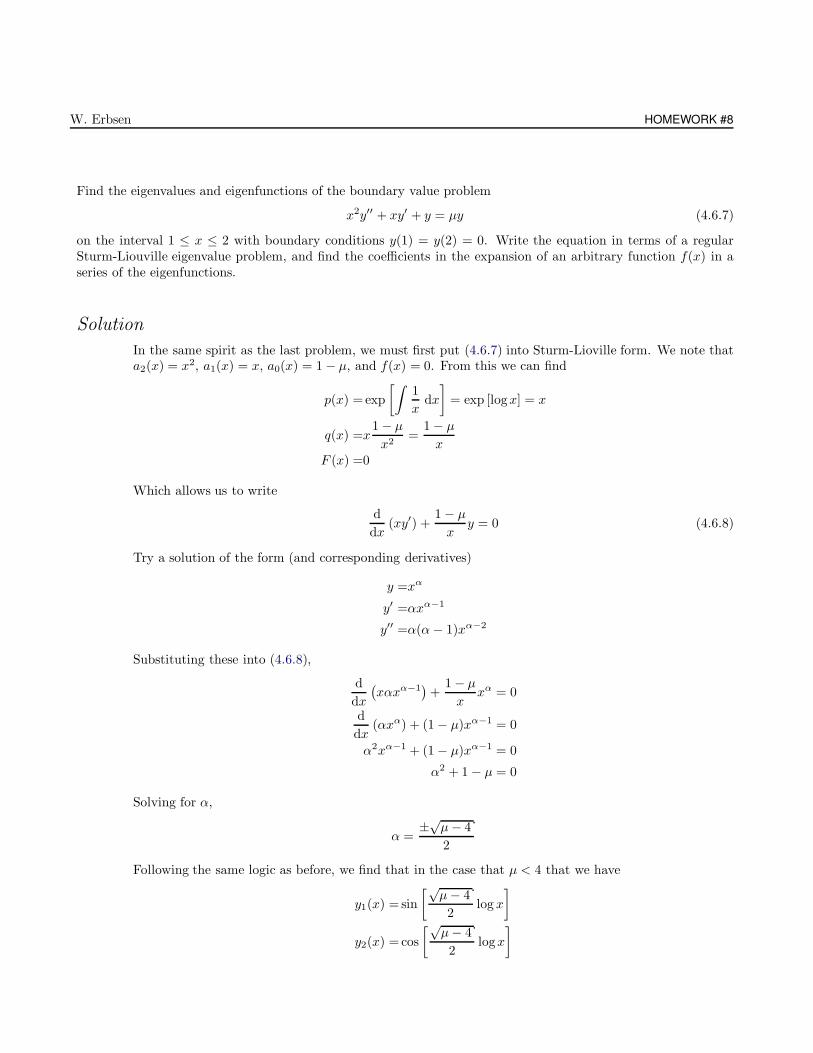
W. Erbsen HOMEWORK #8
Find the eigenvalues and eigenfunctions of the boundary value problem
x2y′′ + xy′ + y = µy (4.6.7)
on the interval 1 ≤ x ≤ 2 with boundary conditions y(1) = y(2) = 0. Write the equation in terms of a regularSturm-Liouville eigenvalue problem, and find the coefficients in the expansion of an arbitrary function f(x) in aseries of the eigenfunctions.
Solution
In the same spirit as the last problem, we must first put (4.6.7) into Sturm-Lioville form. We note thata2(x) = x2, a1(x) = x, a0(x) = 1 − µ, and f(x) = 0. From this we can find
p(x) = exp
[∫1
xdx
]= exp [logx] = x
q(x) =x1 − µ
x2=
1 − µ
xF (x) =0
Which allows us to write
d
dx(xy′) +
1 − µ
xy = 0 (4.6.8)
Try a solution of the form (and corresponding derivatives)
y =xα
y′ =αxα−1
y′′ =α(α− 1)xα−2
Substituting these into (4.6.8),
d
dx
(xαxα−1
)+
1 − µ
xxα = 0
d
dx(αxα) + (1 − µ)xα−1 = 0
α2xα−1 + (1 − µ)xα−1 = 0
α2 + 1 − µ = 0
Solving for α,
α =±√
µ− 4
2
Following the same logic as before, we find that in the case that µ < 4 that we have
y1(x) = sin
[√µ− 4
2log x
]
y2(x) = cos
[√µ− 4
2logx
]
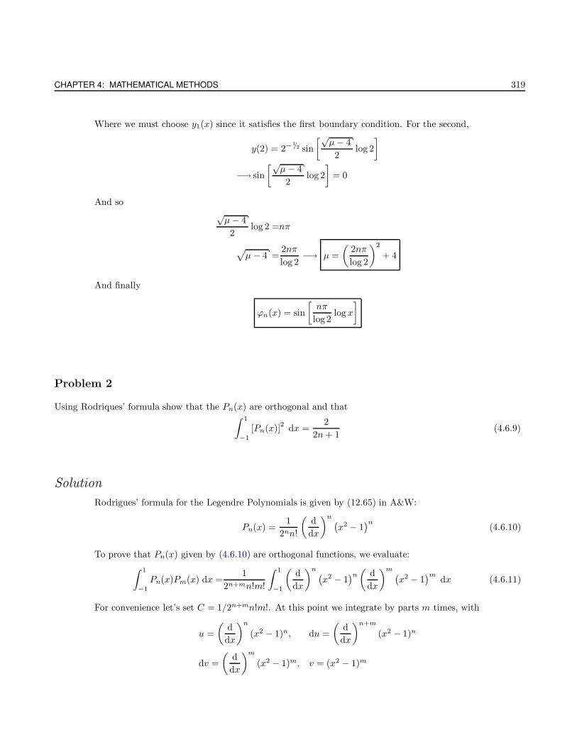
CHAPTER 4: MATHEMATICAL METHODS 319
Where we must choose y1(x) since it satisfies the first boundary condition. For the second,
y(2) = 2−1/2 sin
[√µ− 4
2log 2
]
−→ sin
[√µ− 4
2log 2
]= 0
And so√µ− 4
2log 2 =nπ
√µ − 4 =
2nπ
log 2−→ µ =
(2nπ
log 2
)2
+ 4
And finally
ϕn(x) = sin
[nπ
log 2log x
]
Problem 2
Using Rodriques’ formula show that the Pn(x) are orthogonal and that∫ 1
−1
[Pn(x)]2
dx =2
2n+ 1(4.6.9)
Solution
Rodrigues’ formula for the Legendre Polynomials is given by (12.65) in A&W:
Pn(x) =1
2nn!
(d
dx
)n (x2 − 1
)n(4.6.10)
To prove that Pn(x) given by (4.6.10) are orthogonal functions, we evaluate:
∫ 1
−1
Pn(x)Pm(x) dx =1
2n+mn!m!
∫ 1
−1
(d
dx
)n (x2 − 1
)n(
d
dx
)m (x2 − 1
)mdx (4.6.11)
For convenience let’s set C = 1/2n+mn!m!. At this point we integrate by parts m times, with
u =
(d
dx
)n
(x2 − 1)n, du =
(d
dx
)n+m
(x2 − 1)n
dv =
(d
dx
)m
(x2 − 1)m, v = (x2 − 1)m
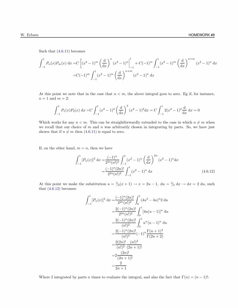
W. Erbsen HOMEWORK #8
Such that (4.6.11) becomes
∫ 1
−1
Pn(x)Pm(x) dx =C
[(x2 − 1)m
(d
dx
)n
(x2 − 1)n
∣∣∣∣1
−1
+ C(−1)m
∫ 1
−1
(x2 − 1)m
(d
dx
)n+m
(x2 − 1)n dx
=C(−1)m
∫ 1
−1
(x2 − 1)m
(d
dx
)n+m
(x2 − 1)n dx
At this point we note that in the case that n < m, the above integral goes to zero. Eg if, for instance,n = 1 and m = 2:
∫ 1
−1
P1(x)P2(x) dx =C
∫ 1
−1
(x2 − 1)2(
d
dx
)3
(x2 − 1)2dx = C
∫ 1
−1
2(x2 − 1)2d
dxdx = 0
Which works for any n < m. This can be straightforwardly extended to the case in which n 6= m whenwe recall that our choice of m and n was arbitrarily chosen in integrating by parts. So, we have justshown that if n 6= m then (4.6.11) is equal to zero.
If, on the other hand, m = n, then we have
∫ 1
−1
[Pn(x)]2 dx =(−1)n
22n(n!)2
∫ 1
−1
(x2 − 1)n
(d
dx
)2n
(x2 − 1)ndx
=(−1)n(2n)!
22n(n!)2
∫ 1
−1
(x2 − 1)n dx (4.6.12)
At this point we make the substitution u = 1/2(x + 1) → x = 2u − 1, du = 1/2 dx → dx = 2 du, suchthat (4.6.12) becomes:
∫ 1
−1
[Pn(x)]2 dx =(−1)n(2n)!
22n(n!)2
∫ 1
0
(4u2 − 4u)n2 du
=2(−1)n(2n)!
22n(n!)2
∫ 1
0
[4u(u− 1)]n du
=2(−1)n(2n)!
(n!)2
∫ 1
0
un(u− 1)n du
=2(−1)n(2n)!
(n!)2(−1)n Γ(n + 1)2
Γ(2n+ 2)
=2(2n)!
(n!)2(n!)2
(2n + 1)!
=2(2n)!
(2n+ 1)!
=2
2n+ 1
Where I integrated by parts n times to evaluate the integral, and also the fact that Γ(n) = (n− 1)!:
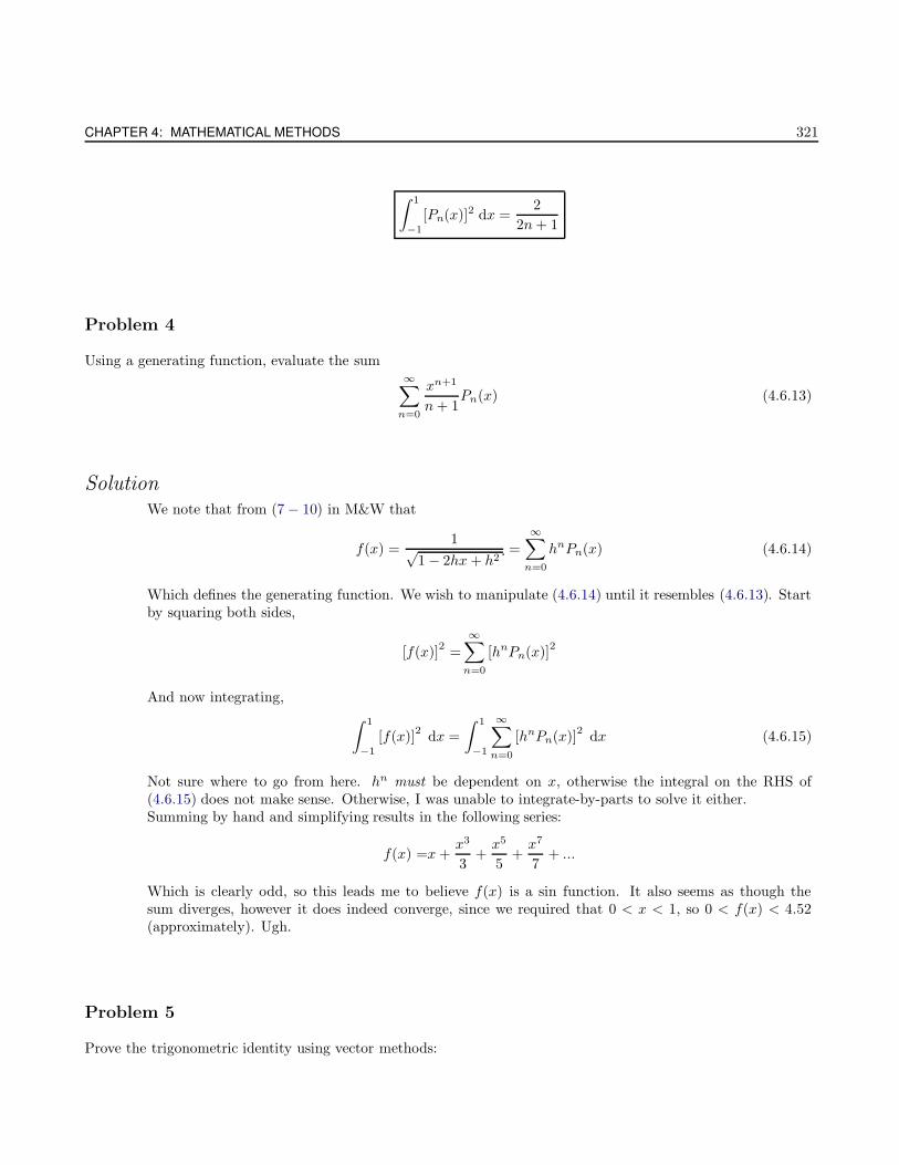
CHAPTER 4: MATHEMATICAL METHODS 321
∫ 1
−1
[Pn(x)]2 dx =2
2n+ 1
Problem 4
Using a generating function, evaluate the sum∞∑
n=0
xn+1
n+ 1Pn(x) (4.6.13)
Solution
We note that from (7 − 10) in M&W that
f(x) =1√
1 − 2hx+ h2=
∞∑
n=0
hnPn(x) (4.6.14)
Which defines the generating function. We wish to manipulate (4.6.14) until it resembles (4.6.13). Startby squaring both sides,
[f(x)]2
=
∞∑
n=0
[hnPn(x)]2
And now integrating,
∫ 1
−1
[f(x)]2
dx =
∫ 1
−1
∞∑
n=0
[hnPn(x)]2
dx (4.6.15)
Not sure where to go from here. hn must be dependent on x, otherwise the integral on the RHS of(4.6.15) does not make sense. Otherwise, I was unable to integrate-by-parts to solve it either.Summing by hand and simplifying results in the following series:
f(x) =x+x3
3+x5
5+x7
7+ ...
Which is clearly odd, so this leads me to believe f(x) is a sin function. It also seems as though thesum diverges, however it does indeed converge, since we required that 0 < x < 1, so 0 < f(x) < 4.52(approximately). Ugh.
Problem 5
Prove the trigonometric identity using vector methods:
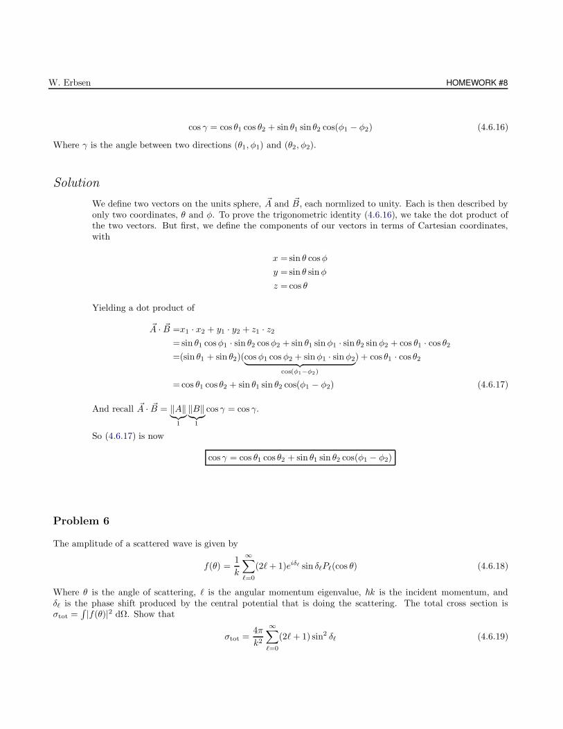
W. Erbsen HOMEWORK #8
cos γ = cos θ1 cos θ2 + sin θ1 sin θ2 cos(φ1 − φ2) (4.6.16)
Where γ is the angle between two directions (θ1, φ1) and (θ2, φ2).
Solution
We define two vectors on the units sphere, ~A and ~B, each normlized to unity. Each is then described byonly two coordinates, θ and φ. To prove the trigonometric identity (4.6.16), we take the dot product ofthe two vectors. But first, we define the components of our vectors in terms of Cartesian coordinates,with
x =sin θ cosφ
y =sin θ sinφ
z =cos θ
Yielding a dot product of
~A · ~B =x1 · x2 + y1 · y2 + z1 · z2=sin θ1 cosφ1 · sin θ2 cosφ2 + sin θ1 sinφ1 · sin θ2 sinφ2 + cos θ1 · cos θ2
=(sin θ1 + sin θ2)(cos φ1 cos φ2 + sinφ1 · sinφ2︸ ︷︷ ︸cos(φ1−φ2)
) + cos θ1 · cos θ2
=cos θ1 cos θ2 + sin θ1 sin θ2 cos(φ1 − φ2) (4.6.17)
And recall ~A · ~B = ‖A‖︸︷︷︸1
‖B‖︸︷︷︸1
cos γ = cos γ.
So (4.6.17) is now
cos γ = cos θ1 cos θ2 + sin θ1 sin θ2 cos(φ1 − φ2)
Problem 6
The amplitude of a scattered wave is given by
f(θ) =1
k
∞∑
`=0
(2`+ 1)eiδ` sin δ`P`(cos θ) (4.6.18)
Where θ is the angle of scattering, ` is the angular momentum eigenvalue, ~k is the incident momentum, andδ` is the phase shift produced by the central potential that is doing the scattering. The total cross section isσtot =
∫|f(θ)|2 dΩ. Show that
σtot =4π
k2
∞∑
`=0
(2` + 1) sin2 δ` (4.6.19)
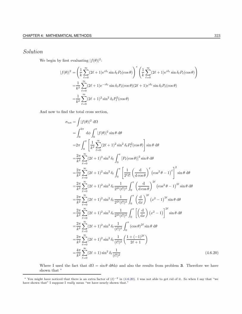
CHAPTER 4: MATHEMATICAL METHODS 323
Solution
We begin by first evaluating |f(θ)|2 :
|f(θ)|2 =
(1
k
∞∑
`=0
(2`+ 1)eiδ` sin δ`P`(cos θ)
)∗(1
k
∞∑
`=0
(2` + 1)eiδ` sin δ`P`(cos θ)
)
=1
k2
∞∑
`=0
(2`+ 1)e−iδ` sin δ`P`(cos θ)(2` + 1)eiδ` sin δ`P`(cos θ)
=1
k2
∞∑
`=0
(2`+ 1)2 sin2 δ`P2` (cos θ)
And now to find the total cross section,
σtot =
∫|f(θ)|2 dΩ
=
∫ 2π
0
dφ
∫ π
0
|f(θ)|2 sin θ dθ
=2π
∫ π
0
[1
k2
∞∑
`=0
(2`+ 1)2 sin2 δ`P2` (cos θ)
]sin θ dθ
=2π
k2
∞∑
`=0
(2` + 1)2 sin2 δ`
∫ π
0
[P`(cos θ)]2sin θ dθ
=2π
k2
∞∑
`=0
(2` + 1)2 sin2 δ`
∫ π
0
[1
2``!
(d
d cos θ
)` (cos2 θ − 1
)`]2
sin θ dθ
=2π
k2
∞∑
`=0
(2` + 1)2 sin2 δ`1
22`(`!)2
∫ π
0
(d
d cos θ
)2` (cos2 θ − 1
)2`sin θ dθ
=2π
k2
∞∑
`=0
(2` + 1)2 sin2 δ`1
22`(`!)2
∫ π
0
(d
dx
)2` (x2 − 1
)2`sin θ dθ
=2π
k2
∞∑
`=0
(2` + 1)2 sin2 δ`1
22`(`!)2
∫ π
0
[(d
dx
)(x2 − 1
)]2`
sin θ dθ
=2π
k2
∞∑
`=0
(2` + 1)2 sin2 δ`1
(`!)2
∫ π
0
(cos θ)2`
sin θ dθ
=2π
k2
∞∑
`=0
(2` + 1)2 sin2 δ`1
(`!)2
(1 + (−1)2`
2`+ 1
)
=4π
k2
∞∑
`=0
(2` + 1) sin2 δ`1
(`!)2(4.6.20)
Where I used the fact that dΩ = sin θ dθdφ and also the results from problem 3. Therefore we haveshown that ∗
∗ You might have noticed that there is an extra factor of (`)−2 in (4.6.20). I was not able to get rid of it. So when I say that “wehave shown that” I suppose I really mean “we have nearly shown that.”
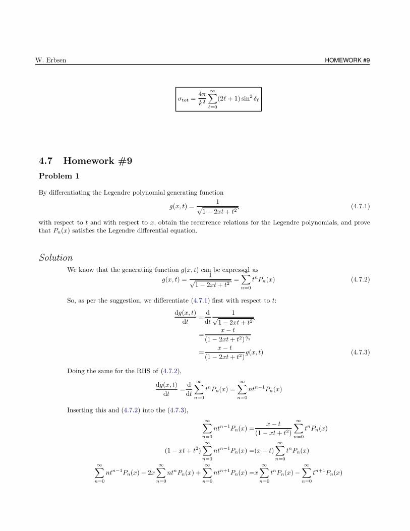
W. Erbsen HOMEWORK #9
σtot =4π
k2
∞∑
`=0
(2`+ 1) sin2 δ`
4.7 Homework #9
Problem 1
By differentiating the Legendre polynomial generating function
g(x, t) =1√
1 − 2xt+ t2(4.7.1)
with respect to t and with respect to x, obtain the recurrence relations for the Legendre polynomials, and provethat Pn(x) satisfies the Legendre differential equation.
Solution
We know that the generating function g(x, t) can be expressed as
g(x, t) =1√
1 − 2xt+ t2=
∞∑
n=0
tnPn(x) (4.7.2)
So, as per the suggestion, we differentiate (4.7.1) first with respect to t:
dg(x, t)
dt=
d
dt
1√1 − 2xt+ t2
=x− t
(1 − 2xt+ t2)3/2
=x− t
(1 − 2xt+ t2)g(x, t) (4.7.3)
Doing the same for the RHS of (4.7.2),
dg(x, t)
dt=
d
dt
∞∑
n=0
tnPn(x) =
∞∑
n=0
ntn−1Pn(x)
Inserting this and (4.7.2) into the (4.7.3),
∞∑
n=0
ntn−1Pn(x) =x− t
(1 − xt+ t2)
∞∑
n=0
tnPn(x)
(1 − xt+ t2)
∞∑
n=0
ntn−1Pn(x) =(x− t)
∞∑
n=0
tnPn(x)
∞∑
n=0
ntn−1Pn(x) − 2x
∞∑
n=0
ntnPn(x) +
∞∑
n=0
ntn+1Pn(x) =x
∞∑
n=0
tnPn(x) −∞∑
n=0
tn+1Pn(x)
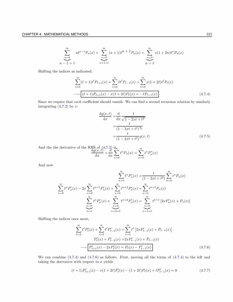
CHAPTER 4: MATHEMATICAL METHODS 325
∞∑
n=0︸︷︷︸n− 1 = `
ntn−1Pn(x) +
∞∑
n=0︸︷︷︸n+1=`
(n+ 1)tn+ 1Pn(x) =
∞∑
n=0︸︷︷︸n = `
x(1 + 2n)tnPn(x)
Shifting the indices as indicated:
∞∑
`=0
(` + 1)t`P`+1(x) +
∞∑
`=0
`t`P`−1(x) =
∞∑
`=0
x(1 + 2`)t`P`(x)
−→ (`+ 1)P`+1(x) − x(1 + 2`)P`(x) = −`P`−1(x) (4.7.4)
Since we require that each coefficient should vanish. We can find a second recursion relation by similarlyintegrating (4.7.2) by x:
dg(x, t)
dx=
d
dx
1√1 − 2xt+ t2
=t
(1 − 2xt+ t2)3/2
=t
(1 − 2xt+ t2)g(x, t) (4.7.5)
And the the derivative of the RHS of (4.7.2) isdg(x, t)
dx=
d
dx
∞∑
n=0
tnPn(x) =
∞∑
n=0
tnP ′n(x)
And now
∞∑
n=0
tnP ′n(x) =
t
(1 − 2xt+ t2)
∞∑
n=0
tnPn(x)
∞∑
n=0
tnP ′n(x) − 2x
∞∑
n=0
tn+1P ′n(x) +
∞∑
n=0
tn+2P ′n(x) =
∞∑
n=0
tn+1Pn(x)
∞∑
n=0︸︷︷︸n=`
tnP ′n(x) +
∞∑
n=0︸︷︷︸n+2=`
tn+2P ′n(x) =
∞∑
n=0︸︷︷︸n+1=`
tn+1 [2xP ′n(x) + Pn(x)]
Shifting the indices once more,
∞∑
`=0
t`P ′`(x) +
∞∑
`=0
t`P ′`−2(x) =
∞∑
`=0
t`[2xP ′
`−1(x) + P`−1(x)]
P ′`(x) + P ′
`−2(x) =2xP ′`−1(x) + P`−1(x)
−→ P ′`+1(x) − 2xP ′
`(x) = P`(x) − P ′`−1(x) (4.7.6)
We can combine (4.7.4) and (4.7.6) as follows. First, moving all the terms of (4.7.4) to the left andtaking the derivative with respect to x yields
(` + 1)P ′`+1(x) − x(1 + 2`)P ′
`(x) − (1 + 2`)P`(x) + `P ′`−1(x) = 0 (4.7.7)
W. Erbsen HOMEWORK #9
Now moving all the terms of (4.7.6) to the left, and multiplying by −`
−`P ′`+1(x) + 2`xP ′
`(x) + `P`(x) − `P ′`−1(x) = 0 (4.7.8)
Adding (4.7.7) and (4.7.8),
P ′`+1(x) = xP ′
`(x) + (1 + `)P`(x)
Many more (in fact, infinitely more) recursion relations may be derived, in addition to the three I havefound here, there are two more that can be found in M&W that become useful:
xP ′`(x) − `P`(x) − P ′
`−1(x) =0 (4.7.9)
P ′`(x) − xP ′
`−1(x) − `P`−1(x) =0 (4.7.10)
Multiplying (4.7.9) by x:
x2P ′`(x) − `xP`(x) − xP ′
`−1(x) = 0 (4.7.11)
(4.7.12)
Now take (4.7.11) and subtract (4.7.10):
x2P ′`(x) − `xP`(x) − xP ′
`−1(x) − P ′`(x) + xP ′
`−1(x) + `P`−1(x) = 0
(x2 − 1)P ′`(x) − `xP`(x) + `P`−1(x) = 0 (4.7.13)
Now taking the derivative of (4.7.13) with respect to x:
2xP ′`(x) + x2P ′′
` (x) − P ′′` (x) − `P`(x) − `xP ′
`(x) + `P ′`−1(x) = 0
x2P ′′` (x) − P ′′
` (x) + (2 − `)xP ′`(x) − `P`(x) + `P`−1(x) = 0 (4.7.14)
At this point we take (4.7.9), solve for P ′`−1(x), and substitute into (4.7.14):
x2P ′′` (x) − P ′′
` (x) + (2 − `)xP ′`(x) − `P`(x) + `xP ′
`(x) − `2P`(x) = 0
(x2 − 1)P ′′` (x) + 2xP ′
`(x) − `xP ′`(x) − `P`(x) + `xP ′
`(x) − `2P`(x) = 0
(x2 − 1)P ′′` (x) + 2xP ′
`(x) − `(` + 1)P`(x) = 0
Which is the Legendre differential equation.
Problem 2
By differentiating the Bessel generating function
g(x, t) = ex2 (t−1/t) (4.7.15)
with respect to t and with respect to x, obtain the recurrence relations for the Bessel functions, and prove thatJn(x) satisfies the Bessel differential equation.
CHAPTER 4: MATHEMATICAL METHODS 327
Solution
In very much the same spirit as the last problem, we are given that the generating function is
g(x, t) = ex2 (t−1/t) =
∞∑
n=0
tnJn(x) (4.7.16)
Differentiating (4.7.15) first with respect to t,
dg(x, t)
dt=
d
dte
x2 (t−1/t)
=x
2
(1 − 1/t2
)e
x2 (t− 1
t )
=x
2
(1 − 1/t2
)g(x, t)
=
∞∑
n=0
ntn−1Jn(x)
Playing with this a little bit, we have
∞∑
n=0
ntn−1Jn(x) =x
2
(1 − 1
t2
) ∞∑
n=0
tnJn(x)
2
∞∑
n=0︸︷︷︸n−1=`
ntn−1Jn(x) =
∞∑
n=0︸︷︷︸n=`
xtnJn(x) −∞∑
n=0︸︷︷︸n−2=`
xtn−2Jn(x)
Shift the indices,
2
∞∑
`=0
(` + 1)t`J`+1(x) =
∞∑
`=0
xt`J`(x) +
∞∑
`=0
t`J`+2
2(`+ 1)J`+1(x) =xJ`(x) + xJ`+2(x)
−→ 2`
xJ`(x) = J`−1(x) + J`+1(x) (4.7.17)
Now differentiating (4.7.15) with respect to x,
dg(x, t)
dx=
d
dxe
x2 (t−1/t)
=1
2
(t− 1
t
)e
x2 (t−1/t)
=1
2
(t− 1
t
)g(x, t)
=∞∑
n=0
tnJ ′n(x)
And now
W. Erbsen HOMEWORK #9
2∞∑
n=0
tnJ ′n(x) =
(t− 1
t
) ∞∑
n=0
tnJn(x)
2
∞∑
n=0︸︷︷︸n=`
tnJ ′n(x) =
∞∑
n=0︸︷︷︸n+1=`
tn+1Jn(x) −∞∑
n=0︸︷︷︸n−1=`
tn−1Jn(x)
Shifting,
2
∞∑
`=0
t`J ′`(x) =
∞∑
`=0
t`J`−1(x) −∞∑
`=0
t`J`+1(x)
−→ 2J ′`(x) = J`−1(x) − J`+1(x) (4.7.18)
If we subtract (4.7.17),
−→ J ′`(x) =
`
xJ`(x) − J`+1(x) (4.7.19)
We can arrive at one more recursion relation if we take (4.7.19) and subtract (4.7.17):
−→ J ′`(x) = J`−1(x) −
`
xJ`(x) (4.7.20)
To prove that Jn(x) satisfies the Bessel differential equation (4.7.15), we start by multiplying (4.7.20) byx:
xJ ′`(x) − xJ`−1(x) + `J`(x) = 0 (4.7.21)
We now differentiate (4.7.21) with respect to x:
d
dx[xJ ′
`(x) − xJ`−1(x) + `J`(x)] =J ′`(x) + xJ ′′
` (x) − J`−1(x) − xJ ′`−1(x) + `J ′
`(x)
=xJ ′′` (x) + (`+ 1)J ′
`(x) − xJ ′`−1(x) − J`−1(x) (4.7.22)
Multiplying (4.7.22) by x,
xJ ′′` (x) + (` + 1)J ′
`(x) − xJ ′`−1(x) − J`−1(x) =0
x2J ′′` (x) + x(`+ 1)J ′
`(x) − x2J ′`−1(x) − xJ`−1(x) =0 (4.7.23)
And multiply (4.7.21) by `:
`xJ ′`(x) − `xJ`−1(x) + `2J`(x) = 0 (4.7.24)
Now take (4.7.22) and subtract (4.7.21):
x2J ′′` (x) + x(`+ 1)J ′
`(x) − x2J ′`−1(x) − xJ`−1(x) − `xJ ′
`(x) + `xJ`−1(x) − `2J`(x) =0
x2J ′′` (x) + xJ ′
`(x) − x2J ′`−1(x) + (`− 1)J`−1(x) − `2J`(x) =0 (4.7.25)
At this point we take (4.7.19) and shift the index from ` to ` − 1,
CHAPTER 4: MATHEMATICAL METHODS 329
J ′`−1(x) =
` − 1
xJ`−1(x) − J`(x)
And multiplying this by x and solving for J`−1(x),
xJ ′`−1(x) = (` − 1)J`−1(x) − xJ`(x) −→ J`−1(x) =
x
`− 1J ′
`−1(x) +x
`− 1J`(x)
Substituting this into (4.7.25),
x2J ′′` (x) + xJ ′
`(x) − x2J ′`−1(x) + (` − 1)
[x
`− 1J ′
`−1(x) +x
`− 1J`(x)
]− `2J`(x) =0
x2J ′′` + xJ ′
`(x) − x2J ′`−1(x) + x2J`−1(x) + x2J`(x) − `2J` = 0
x2J ′′` (x) + xJ ′
`(x) +(x2 − `2
)J`(x) = 0
Which is the Bessel differential equation.
Problem 3
Prove the normalization condition for the Bessel functions∫ ∞
0
·Jn(kr) · Jn(k′r) drr =1
kδ(k′ − k) (4.7.26)
Solution
It was shown in class, and additionally can be found in M&W that:
∫ b
a
Jn(αr)Jn(βr)rdr =1
α2 − β2[βrJn(αr)J ′
n(βr) − αrJn(βr)J ′n(αr)|ba (4.7.27)
Where I dispensed k and k′ in favor of α and β, respectively in order to avoid confusion with thederivatives. First let’s choose a→ 0 as in (4.7.26):
∫ b
0
Jn(αr)Jn(βr)rdr =1
α2 − β2[βrJn(αr)J ′
n(βr) − αrJn(βr)J ′n(αr)|b0
=1
α2 − β2[βrJn(αb)J ′
n(βb) − αrJn(βb)J ′n(αb)] (4.7.28)
And since both J ′`(αr) and J ′
`(βr) evaluated at the endpoints equal zero, then (4.7.36) too must vanish.To see that this is the case at x = 0, it is illuminating to recall that J ′
`(0) = J`+1(0) = 0. We shouldalso recognize that J ′
`(∞) → 0. Both of these properties become very evident when plotting the relevantfunctions and recognizing the respective behaviors. Therefore, (4.7.28) becomes
W. Erbsen HOMEWORK #9
∫ b
0
Jn(αr)Jn(βr)rdr = 0 (4.7.29)
For the case in which α and β are equal, we must evaluate
∫ b
0
Jn(αr)Jn(βr)rdr =
∫ b
0
Jn(αr)Jn(αr)rdr =
∫ b
0
[Jn(αr)]2rdr
Which we now set equal to the RHS of (4.7.28)
∫ b
0
[Jn(αr)]2rdr =
βrJn(αb)J ′n(βb) − αrJn(βb)J ′
n(αb)
α2 − β2(4.7.30)
Evaluating the RHS of (4.7.30) is not so easy; we must take the limit as β → α, but since this isindeterminate we must use L’Hospital’s Rule:
∫ b
0
[Jn(αr)]2r dr = lim
β→α
[βrJn(αb)J ′
n(βb) − αrJn(βb)J ′n(αb)
α2 − β2
]
= limβ→α
[rJn(αb)J ′
n(βb) + βrJn(αb)J ′′n(βb) − αrJ ′
n(βb)J ′n(αb)
−2β
]
=αr [J ′
n(αb)]2 − rJn(αb)J ′
n(αb) − αrJn(αb)J ′′n(αb)
2α(4.7.31)
We now solve Bessel’s differential equation for J ′′n(αb):
α2J ′′n(αb) + αJ ′
n(αb) + (α2 − n2)Jn(αb) = 0 −→ J ′′n(αb) = −αJ
′n(αb) − (α2 − n2)Jn(αb)
α2(4.7.32)
Substituting (4.7.32) into (4.7.31),
∫ b
0
[Jn(αr)]2rdr =
αr [J ′n(αb)]
2 − rJn(αb)J ′n(αb) − αrJn(αb)
[−αJ′
n(αb)−(α2−n2)Jn(αb)α2
]
2α
=αr [J ′
n(αb)]2 − rJn(αb)J ′
n(αb) + rJn(αb)J ′n(αr) + αr
(1 − n2
α2
)[Jn(αb)]
2
2α
=r
2
[[J ′
n(αb)]2
+
(1 − n2
α2
)[Jn(αb)]
2
](4.7.33)
So that if α and β represent two unique roots of order n then (4.7.33) must vanish.
Problem 4
A disk of radius R in the xy-plane (z = 0) is kept at a constant potential φ0 and the rest of the plane z = 0 iskept at zero potential. As shown in class, the potential for z > 0 is given by
φ(r, z) = φ0R
∫ ∞
0
dkJ1(kR)J0(kr)e−kz (4.7.34)
CHAPTER 4: MATHEMATICAL METHODS 331
Hence, the potential above the center of the disk (r = 0) is given by the integral
φ(0, z) = φ0R
∫ ∞
0
dkJ1(kR)e−kz (4.7.35)
Using the Bessel function recurrence relations and the integral representation of the Bessel function, show that thelast expression can be reduced to
φ(0, z) = φ0
[1 − z√
z2 +R2
](4.7.36)
Solution
According to (4.7.19),
J1(x) = −J ′0(x)
And (4.7.35) becomes
φ(0, z) = −φ0R
∫ ∞
0
J ′0(kR)e−kz dk
And at this point we wish to undergo a change of variables x = kR −→ k = x/R:
φ(0, z) = − φ0R
∫ ∞
0
J ′0(x)e
−xz/Rdx
R
= − φ0
∫ ∞
0
J ′0(x)e
−xz/R dx
Where we must integrate by parts:
u = e−xz/R , du = − z
Re−
xz/R
dv = J ′0(x), v = J0(x)
So we now have
φ(0, z) = − φ0
[J0(x)e
−xz/R
∣∣∣∞
0+z
R
∫ ∞
0
J0(x)e−xz/R dx
= − φ0
−1 +
z
R
∫ ∞
0
J0(x)e−xz/R dx
(4.7.37)
At this point we pause, try a myriad of obscure substitutions, get frustrated, have a beer, and thenrealize that the integral in (4.7.37) has actually been tabulated by the likes of Gradshteyn and Ryzhikas Eq. 6.611.1: ?
∫ ∞
0
e−αxJν(βx) dx =β−ν
[√α2 + β2 − α
]ν
√α2 + β2
Where in our case α = z/R, β = 1 and ν = 0:
W. Erbsen HOMEWORK #10
∫ ∞
0
e−xz/RJ0(x) dx =
1√(z/R)
2+ 1
=1
1/R√z2 +R2
=R√
z2 + R2(4.7.38)
And substituting (4.7.38) into (4.7.37),
φ(0, z) = − φ0
−1 +
z
R
(R√
z2 + R2
)
From which we finally arrive at (4.7.36), thus completing the problem:
φ(0, z) = φ0
1 − z√
z2 + R2
4.8 Homework #10
Problem 1
In class we shows that the lowest order spherical Bessel function is given by
j0(x) =sinx
x(4.8.1)
Using the recurrence relations, find j1(x) and j2(x), and also prove that
j`(x) = (−1)`x`
(1
x
∂
∂x
)`
j0(x) (4.8.2)
Solution
Recall that one of the recurrence relations for Bessel functions reads
j`+1(x) =`
xj`(x) − j′`(x) (4.8.3)
Which was rigorously proven in Homework #9, and subsequently will be treated as an axiom in thisassignment. We are given j0(x), so we need to calculate j1(x) and j2(x) using our recursion relation(4.8.3). We start by finding the first derivative of (4.8.1):
j′0(x) =cosx
x− sinx
x2
We now substitute this into (4.8.3),
j1(x) =0
xj0(x) − j′0(x)
=sinx
x2− cosx
x(4.8.4)
CHAPTER 4: MATHEMATICAL METHODS 333
Taking the first derivative of j1(x) yields
j′1(x) =2 cosx
x2− 2 sinx
x3+
sinx
x
From which we can now find j2(x):
j2(x) =1
xj1(x) − j′1(x)
=sinx
x3− cosx
x2− 2 cosx
x2+
2 sinx
x3− sinx
x
=3 sinx
x3− 3 cosx
x2− sinx
x(4.8.5)
In order to prove (4.8.2), it will be most convenient to show that (4.8.2) works when substituted into(4.8.3). I will employ proof by induction. So the first step is to show that it works for ` = 0,
j1(x) = − j′0(x)
= − d
dx
[(−1)0x0
(1
x
∂
∂x
)0
j0(x)
]
= − d
dx
sinx
x
=sinx
x2− cosx
x
=j1(x) X
So it works for ` = 0. Assuming that it holds for all `, we now show that it holds for ` + 1. First findthe derivative of j`(x):
j′`(x) =d
dx
[(−x)`
(1
x
d
dx
)`sinx
x
]
=
[d
dx(−x)`
] [(1
x
d
dx
)`sinx
x
]+ (−x)` d
dx
[(1
x
d
dx
)`sinx
x
]
=`(−x)`−1
[(1
x
d
dx
)`sinx
x
]+ (−x)` d
dx
[(1
x
d
dx
)`sinx
x
]
= − `(−x)`
x
[(1
x
d
dx
)`sinx
x
]+ (−x)` d
dx
[(1
x
d
dx
)`sinx
x
]
= − `
x(−x)`
[(1
x
d
dx
)`sinx
x
]+ (−x)` d
dx
[(1
x
d
dx
)`sinx
x
]
= − `
xj`(x) + (−x)` d
dx
[(1
x
d
dx
)`sinx
x
](4.8.6)
So, let’s find j`+1(x):
j`+1(x) =(−x)`+1
(1
x
d
dx
)`+1sinx
x
W. Erbsen HOMEWORK #10
=(−x)`(−x)(
1
x
d
dx
)`(1
x
d
dx
)sinx
x
= − (−x)` d
dx
[(1
x
d
dx
)`sinx
x
]
=`
xj`(x) − j′`(x) X
Where I used (4.8.6). Since (4.8.2) works for ` = 0 (the base step) and also ` + 1 (the inductive step),then it follows that it works for ` (the hypothesized step).
Problem 2
Using the definition of Neumann functions in terms of Bessel functions, show that for the spherical Neumannfunctions,
η0(x) = −cos x
x(4.8.7)
Using the recurrence relations, find η1(x) and η2(x).
Solution
Analogous to (4.8.3), the recursion relation for the Neumann functions takes the form
η`+1(x) =`
xη`(x) − η′`(x) (4.8.8)
So, from ` = 0 we can find η1(x):
η1(x) =`
xη0(x) − η′0(x) =⇒= −η′0(x) (4.8.9)
So, in finding the first derivative of η0(x), we find η1(x):
η1(x) = −η′0(x) =d
dx
cosx
x= −sinx
x− cosx
x2(4.8.10)
Applying the same process letting ` = 1,
η1+1(x) =1
xη1(x) − η′1(x)
= − sinx
x2− cosx
x3− η′1(x) (4.8.11)
Where we find that
η′1(x) =d
dx
[−sinx
x− cos x
x2
]
= − cosx
x+
2 sinx
x2+
sinx
x2+
2 cosx
x3
CHAPTER 4: MATHEMATICAL METHODS 335
= − cosx
x+
2 sinx
x2+
2 cosx
x3(4.8.12)
Substituting (4.8.12) into (4.8.11), we find that
η2(x) = − sinx
x2− cosx
x3+
cosx
x− 2 sinx
x2− 2 cosx
x3
=cosx
x− 3 sinx
x3− 3 cosx
x3(4.8.13)
Problem 3
Transform the hyperbolic equation
y2ψxx − x2ψyy = 0 (4.8.14)
into the canonical form of ψην = f(...)
Solution
The general formalism of the Method of Characteristics entails taking some arbitrary differential equation,
Au2xx + 2Buxy + Cu2
yy = 0 −→ Au2ξξ + 2Buξη + Cu2
ηη + R = 0 (4.8.15)
WhereA =Aξ2x + 2Bξxξy +Cξ2y
B =Aξxηx + B (ξxηy + ξyηx) +Cξyηy
C =Aη2x + 2Bηxηy + Cη2
y
R =(Aξxx + 2Bξxy +Cξyy)uξ + (Aηxx + 2Bηxy +Cηyy)uη
So, from (4.8.14), it is apparent that A = y2, B = 0, and C = −x2. Since (4.8.14) is hyperbolic, thecharacteristics can be found by
dy
dx=B ±
√B2 − 4AC
2A= ±
√−4AC
2A= ±x
y
Solving and integrating this we arrive at
x2
2± y2
2= 0 −→ x2 ± y2 = 0 (4.8.16)
Where we now define
ξ(x, y) = ξ = x2 + y2 , and η(x, y) = η = x2 − y2 (4.8.17)
Taking some partial derivatives,
ξx =2x, ξy = 2y, ξxx = ξyy = 2, ξxy = 0
W. Erbsen HOMEWORK #10
ηx =2x, ηy = −2y, ηxx = 2, ηyy = −2, ηxy = 0
Now finding the coefficients in (4.8.15),
A =Aξ2x + 2Bξxξy +Cξ2y
=y2ξ2x − x2ξ2y
=y2(2x)2 − x2(2y)2 = 0
B =Aξxηx + B (ξxηy + ξyηx) +Cξyηy
=y2ξxηx − x2ξyηy
=y2(2x)(2x)− x2(2y)(−2y)
=4x2y2 + 4x2y2
=8x2y2
C =Aη2x + 2Bηxηy + Cη2
y
=y2η2x − x2η2
y
=y2(2x)2 − x2(−2x)2
=0
R =(Aξxx + 2Bξxy +Cξyy)uξ + (Aηxx + 2Bηxy +Cηyy)uη
=(y2ξxx − x2ξyy
)uξ +
(y2ηxx − x2ηyy
)uη
=2(y2 − x2
)uξ + 2
(y2 + x2
)uη
And putting all these into (4.8.15),
Au2ξξ + 2Buξη + Cu2
ηη + R = 0
2(8x2y2)uξη + 2(y2 − x2
)uξ + 2
(y2 + x2
)uη = 0
8x2y2uξη +(y2 − x2
)uξ +
(y2 + x2
)uη = 0 (4.8.18)
We can combine our original definitions of ξ and η from (4.8.17) to obtain:
x2 =ξ + η
2, and y2 =
ξ − η
2
So that we can now rewrite (4.8.18) as
8
(ξ + η
2
)(ξ − η
2
)uξη − ηuξ + ξuη = 0
2(ξ2 − η2
)uξη − ηuξ + ξuη = 0
And the canonical form of (4.8.14) becomes
uξη =ηuξ − ξuη
2 (ξ2 − η2)
CHAPTER 4: MATHEMATICAL METHODS 337
Problem 4
Transform the elliptical equations
y2ψxx + x2ψyy = 0 (4.8.19a)
ψxx + (1 + y)2ψyy = 0 (4.8.19b)
into the canonical form of ψσσ + ψττ = f(...).
Solution
Starting from (4.8.19a), it is apparent to the casual observer that A = y2, B = 0 and C = x2. Further-more, we can go on to find the characteristics of this equation:
dy
dx=
−B ±√B2 − 4AC
2A=
√−ACA
=ix
y(4.8.20)
Solving and integrating, we find that
ix2
2± y2
2= 0 −→ ix2 ± y2 = 0 (4.8.21)
At this point we set
ξ(x, y) = ξ = ix2 + y2 , and η(x, y) = η = ix2 − y2 (4.8.22)
With corresponding partial derivatives
ξx =2ix, ξy = 2y, ξxx = 2i, ξyy = 2, ξxy = 0
ηx =2ix, ηy = −2y, ηxx = 2i, ηyy = −2, ηxy = 0
And now finding the coefficients,
A =Aξ2x + 2Bξxξy +Cξ2y
=y2(2ix)2 + x2(2y)2
= − 4x2y2 + 4x2y2
=0
B =Aξxηx + B (ξxηy + ξyηx) +Cξyηy
=y2(2ix)(2ix) + x2(2y)(−2y)
= − 4x2y2 − 4x2y2
= − 8x2y2
C =Aη2x + 2Bηxηy + Cη2
y
=y2(2ix)2 + x2(−2y)2
= − 4x2y2 + 4x2y2
W. Erbsen HOMEWORK #10
=0
R =(Aξxx + 2Bξxy +Cξyy)uξ + (Aηxx + 2Bηxy +Cηyy)uη
=(y2(2i) + x2(2)
)uξ +
(y2(2i) + x2(−2)
)uη
=2(iy2 + x2
)uξ + 2
(iy2 − x2
)uη
Substituting these in we have
2Buξη + R = 0
− 16x2y2uξη + 2(iy2 + x2
)uξ + 2
(iy2 − x2
)uη = 0 (4.8.23)
And it is possible to eliminate x and y by making the following substitution:
x2 =ξ + η
2i, and y2 =
ξ − η
2
Putting this in (4.8.23) and simplifying,
−16
(ξ2 − η2
4i
)uξη − 2iηuξ + 2iξuη
2(ξ2 − η2
)uξη − ηuξ + ξuη = 0
From which we finally arrive at
uξη =ηuξ − ξuη
2 (ξ2 − η2)
In the same spirit for (4.8.19b), we note that A = 1, B = 0, C = (1 + y)2 . Finding the characteristics,
dy
dx=
−B ±√B2 − 4AC
2A=
±√−ACA
= ±i(1 + y) (4.8.24)
Solving and integrating,
1
1 + ydy = ±i dx −→ log (1 + y) = ±ix
Assigning our two independent variables,
ξ(x, y) = ξ = ix+ log (1 + y), and η(x, y) = η = ix − log (1 + y) (4.8.25)
Let’s take some partial derivatives:
ξx =i, ξy =1
1 + y, ξxx = 0, ξyy = − 1
(1 + y)2, ξxy = 0
ηx =i, ηy = − 1
1 + y, ηxx = 0, ηyy =
1
(1 + y)2, ηxy = 0
And the coefficients are
CHAPTER 4: MATHEMATICAL METHODS 339
A =Aξ2x + 2Bξxξy +Cξ2y
=Aξ2x + (1 + y)2ξ2y
=(i)(i) + (1 + y)21
(1 + y)2
= − 1 + 1
=0
B =Aξxηx + B (ξxηy + ξyηx) +Cξyηy
=ξxηx + (1 + y)2ξyηy
=(i)(i) + (1 + y)2(
1
1 + y
)(− 1
1 + y
)
= − 1 − 1
= − 2
C =Aη2x + 2Bηxηy + Cη2
y
=η2x + (1 + y)2η2
y
=(i)(i) + (1 + y)2(
1
1 + y
)2
= − 1 + 1
=0
R =(Aξxx + 2Bξxy +Cξyy)uξ + (Aηxx + 2Bηxy +Cηyy)uη
=(1 + y)2ξyyuξ + (1 + y)2ηyyuη
=(1 + y)2(− 1
(1 + y2)2
)uξ + (1 + y)2
(1
(1 + y)2
)uη
= − uξ + uη
And now we can find the canonical form of (4.8.19b):
2Buξη +R = 0
− 4uξη − uξ + uη = 0
And finally
uξη =uξ − uη
4
W. Erbsen HOMEWORK #10
Problem 5
Classify the following equations in appropriate regions and transform them into canonical form:
ψxx − y2ψyy + ψx − ψ + x2 = 0 (4.8.26a)
ψxx + xψyy = 0 (4.8.26b)
Solution
For (4.8.26a) it is important that the elements that characterize the dominant behavior are the secondorder terms, so analyzing this (the principle part), we see that A = 1, B = 0, and C = −y2 . Furthermore,we can see that:
B2 − AC = y2 > 0 −→ hyperbolic
Solving, integrating:
dy
dx= ±y −→ x± log y = 0
And now we can say
ξ(x, y) = ξ = x+ log y, and η(x, y) = η = x− log y
Take some partials:
ξx =1, ξy =1
y, ξxx = 0, ξyy = − 1
y2, ξxy = 0
ηx =1, ηy = −1
y, ηxx = 0, ηyy =
1
y2, ηxy = 0
And the coefficients are
A =Aξ2x + 2Bξxξy +Cξ2y
=ξ2x − y2ξ2y
=1 − y2 1
y2
=1 − 1
=0
B =Aξxηx + B (ξxηy + ξyηx) +Cξyηy
=ξxηx − y2ξyηy
=1 − y2
(1
y
)(1
y
)
=1 + 1
=2
CHAPTER 4: MATHEMATICAL METHODS 341
C =Aη2x + 2Bηxηy + Cη2
y
=η2x − y2η2
y
=1 − y2
(−1
y
)2
=1 − 1
=0
R =(Aξxx + 2Bξxy +Cξyy)uξ + (Aηxx + 2Bηxy +Cηyy)uη
=(ξxx − y2ξyy
)uξ +
(ηxx − y2ηyy
)uη
=
[1 − y2
(1
y
)]uξ +
[1 − y2
(−1
y
)]uη
=(1 − y) uξ + (1 + y) uη
And we now have
4uξη + (1 − y) uξ + (1 + y) uη = 0
And consequently
4uξη +
(1 − exp
[ξ − η
2
])uξ +
(1 +
[ξ − η
2
])uη = 0
This last equation yields A = 1, B = 0, C = x, which is elliptical, assuming that x > 0:
B2 −AC = −x < 0 −→ elliptical
Find the characteristics:
dy
dx= ±
√−x = ±i
√x
Solving and integrating, we arrive at
ξ(x, y) = ξ =2
3ix
3/2 + y, and η(x, y) = η =2
3ix
3/2 − y
With partial derivatives
ξx =i√x , ξy = 1, ξxx =
1
2√x, ξyy = 0, ξxy = 0
ηx =√x , ηy = −1, ηxx =
1
2√x, ηyy = 0, ηxy = 0
Finding the coefficients
A =Aξ2x + 2Bξxξy +Cξ2y
=ξ2x + xξ2y
W. Erbsen HOMEWORK #11
=(i√x )2 + x
= − x+ x
=0
B =Aξxηx + B (ξxηy + ξyηx) +Cξyηy
=(i√x )(i
√x ) + x(1)(−1)
= − x− x
= − 2x
C =Aη2x + 2Bηxηy + Cη2
y
=(√x )2 + x(−1)2
=x− x
=0
R =(Aξxx + 2Bξxy +Cξyy)uξ + (Aηxx + 2Bηxy +Cηyy)uη
=(ξxx + xξyy)uξ + (ηxx + xηyy)uη
=
(i
2√x
)uξ +
(i
2√x
)uη
Our equation becomes
− 4xuξη +i
2√x
(uξ + uη) = 0
And finally
−4
[3
4i(ξ − η)
]2/3
uξη +i
2
[4i
3
1
ξ − η
]1/3
(uξ + uη) = 0
4.9 Homework #11
Problem 1
Consider a thin half pipe of unit radius laying on the ground. It is heated by radiation from above. We takethe initial temperature of the pipe and the temperature of the ground to be zero. We model this problem with aheat equation with a source term.
ut = κuxx + A sinx, u(0, t) = u(π, t) = 0, u(x, 0) = 0 (4.9.1)
CHAPTER 4: MATHEMATICAL METHODS 343
Solution
We begin by assuming that our solution can be written in terms of a steady-state solution and a transientone
u(x, t) = µ(x) +w(x, t) µ(x) : Steady-state solutionw(x, t) : Transient solution
To find the equilibrium solution, we note that µt(x) = 0, and substitute µ(x) into (4.9.1):
µt = κµxx +A sinx −→ µxx = −Aκ
sinx, µ(0) = µ(π) = 0 (4.9.2)
Integrating (4.9.2) once,
∫ x
0
∂2
∂x2µ(x) dx = − A
κ
∫ x
0
sinx dx
∂
∂xµ(x) =
A
κcos x+C1 (4.9.3)
And now integrating (4.9.3),
∫ x
0
∂
∂xµ(x) dx =
A
κ
∫ x
0
cosx dx+
∫ x
0
C1 dx
µ(x) =A
κsinx+ C1x+ C2 (4.9.4)
Applying our first boundary condition to (4.9.4), we find that
µ(0) =C2 6= 0 −→ C2 = 0
And similarly, applying th4e second boundary condition,
µ(π) =C1π 6= 0 −→ C1 = 0
And (4.9.4) becomes
µ(x) =A
κsinx (4.9.5)
And now we do the same for w(x, t):
wt = κwxx +A sinx −→ wt = κwxx (4.9.6)
We can see that (4.9.6) can be expressed as an eigenvalue problem, the explicit details of which are shownin subsequent problems and I will not repeat them here. Applying all our given conditions, we arrive at
wn(x, t) =
√2
πsin (nx) e−κn2t (4.9.7)
And in order for (4.9.7) to work, we require that it corresponds to the Fourier coefficient an fromw(x, t) =
∑anwn(x, t):
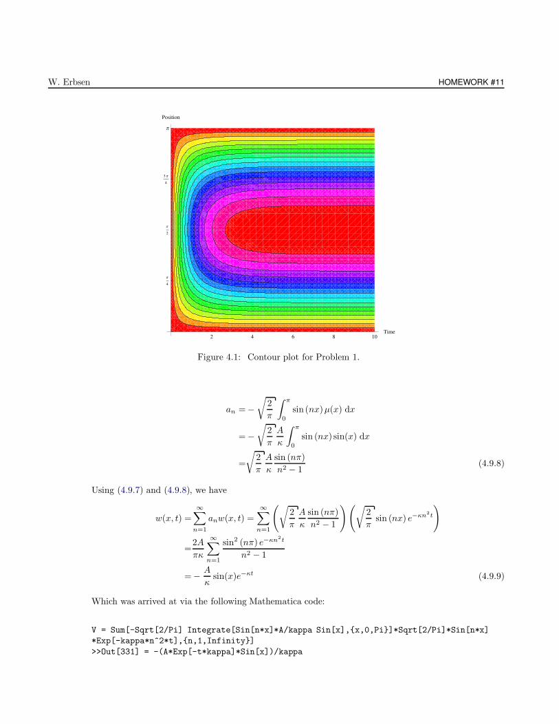
W. Erbsen HOMEWORK #11
2 4 6 8 10Time
Π
4
Π
2
3 Π
4
Π
Position
Figure 4.1: Contour plot for Problem 1.
an = −√
2
π
∫ π
0
sin (nx)µ(x) dx
= −√
2
π
A
κ
∫ π
0
sin (nx) sin(x) dx
=
√2
π
A
κ
sin (nπ)
n2 − 1(4.9.8)
Using (4.9.7) and (4.9.8), we have
w(x, t) =
∞∑
n=1
anw(x, t) =
∞∑
n=1
(√2
π
A
κ
sin (nπ)
n2 − 1
)(√2
πsin (nx) e−κn2t
)
=2A
πκ
∞∑
n=1
sin2 (nπ) e−κn2t
n2 − 1
= − A
κsin(x)e−κt (4.9.9)
Which was arrived at via the following Mathematica code:
V = Sum[-Sqrt[2/Pi] Integrate[Sin[n*x]*A/kappa Sin[x],x,0,Pi]*Sqrt[2/Pi]*Sin[n*x]
*Exp[-kappa*n^2*t],n,1,Infinity]
>>Out[331] = -(A*Exp[-t*kappa]*Sin[x])/kappa
CHAPTER 4: MATHEMATICAL METHODS 345
And finally, to get the full solution for u(x, t) we combine our steady-state solution from (4.9.5) and ourtransient solution from (4.9.9):
u(x, t) = w(x, t) + µ(x) = −Aκ
sin(x)e−κt +A
κsin(x)
Which may be rewritten as
u(x, t) =A
κsin(x)
[1 − e−κt
]
A contour plot of my solution can be seen in Fig. (4.1), where I set A = κ = 1.
Problem 2
Obtain Poisson’s formula to solve the Dirichlet problem for the circular region 0 ≤ r < R, 0 ≤ θ < 2π. That is,determine a solution φ(r, θ) to solve Laplace’s equation ∇2φ = 0 in polar coordinates given φ(R, θ). Show that
φ(r, θ) =1
2π
∫ 2π
0
φ(R, α)R2 − r2
R2 + r2 − 2Rr cos (θ − α)dα (4.9.10)
Solution
We begin by noting that Laplace’s equation in polar coordinates is
∇2f =1
r
∂
∂r
(r∂f
∂r
)+
1
r2∂2f
∂θ2= 0 (4.9.11)
Which should be solvable using separation of variables, where we assume that the solution can take theform of f(r, θ) = R(r)Θ(θ). Substituting this into (4.9.11) and separating the variables,
r
R
d
dr
(rdR
dr
)= − 1
Θ
d2Θ
dθ2= λ2 (4.9.12)
Where we set each equation equal to the square of some equilibrium constant λ. We first take theequation for R(r),
r
R
d
dr
(rdR
dr
)=λ2
r
R
[rd2R
dr2+
dR
dr
]=λ2
r2d2R
dr2+ r
dR
dr− λ2R =0 (4.9.13)
Now we must solve the equation for Θ(θ) from (4.9.12):
W. Erbsen HOMEWORK #11
− 1
Θ
d2Θ
dθ2=λ2
d2Θ
dθ2+ λ2Θ =0 (4.9.14)
We require our solution for Θ(θ) to be periodic, such that Θ(θ + 2π) = Θ(θ). Therefore we set λ = nwhere n is an integer, and (4.9.14) becomes
d2Θ
dθ2+ n2Θ =0
Which has solutions
Θ(θ) =Aneinθ +Bne
−inθ = An cos(nθ) + Bn sin(nθ) (4.9.15)
And similarly we can rewrite (4.9.13) as
r2d2R
dr2+ r
dR
dr− n2R =0
Which has solutions of the form
R(r) = Cnrn +Dnr
−n (4.9.16)
Combining our solutions from (4.9.15) and (4.9.16),
fn(r, θ) = R(r)Θ(θ) =(Cnr
n +Dnr−n)(An cos(nθ) + Bn sin(nθ))
Choosing Dn = 0 for boundary conditions,
fn(r, θ) = Cnrn (An cos(nθ) + Bn sin(nθ))
And more generally,
fn(r, θ) =
∞∑
n=0
Cnrn (An cos(nθ) + Bn sin(nθ))
=C0r0 (A0 cos(0) +B0 sin(0)) +
∞∑
n=1
Cnrn (An cos(nθ) +Bn sin(nθ))
=C0A0 +
∞∑
n=1
Cnrn (An cos(nθ) +Bn sin(nθ)) (4.9.17)
The solution of (4.9.17) is most easily found if we first assume that R = r = 1,
f(1, θ) =C0A0 +
∞∑
n=1
Cn (An cos(nθ) +Bn sin(nθ))
=a0 +
∞∑
n=1
(an cos(nθ) + bn sin(nθ)) (4.9.18)
CHAPTER 4: MATHEMATICAL METHODS 347
Where I have set C0A0 = a0, Cn = 1, An = an and Bn = bn. In doing this, we see that (4.9.18) is justa Fourier series. The coefficients are readily determined with
a0 =1
2· 1
π
∫ 2π
0
f(1, α) dα (4.9.19a)
an =1
π
∫ 2π
0
f(1, α) cos(nα) dα (4.9.19b)
bn =1
π
∫ 2π
0
f(1, α) sin(nα) dα (4.9.19c)
Substituting (4.9.19a), (4.9.19b) and (4.9.19c) into (4.9.18):
f(1, θ) =a0 +
∞∑
n=1
(an cos(nθ) + bn sin(nθ))
=1
2π
∫ 2π
0
f(1, α) dα+
∞∑
n=1
(1
π
∫ 2π
0
f(1, α) cos(nα) dα cos(nθ) +1
π
∫ 2π
0
f(1, α) sin(nα) dα sin(nθ)
)
=1
π
∫ 2π
0
[1
2f(1, α) +
∞∑
n=1
(f(1, α) cos(nα) cos(nθ) + f(1, α) sin(nα) sin(nθ))
]dα
=1
π
∫ 2π
0
f(1, α)
[1
2+
∞∑
n=1
(cos(nα) cos(nθ) + sin(nα) sin(nθ))
]dα
=1
π
∫ 2π
0
f(1, α)
[1
2+
∞∑
n=1
cos [n (θ − α)]
]dα (4.9.20)
Where I used the identity cosα cosβ + sinα sinβ = cos (α− β) = cos (β − α). The bracketed term in(4.9.20) can be simplified, and I used Mathematica:
FullSimplify[1/2 + Sum[r^n*Cos[n*(alpha - theta], n, 1, Infinity]]
>>Out[157]=-((-1 + r^2)/(2*(1 + r^2 - 2*r*Cos[alpha - theta])))
With this, (4.9.20) becomes
f(1, θ) =1
π
∫ 2π
0
f(1, α)
[1 − r2
2 (1 + r2 − 2r cos (θ − α))
]dα
=1
2π
∫ 2π
0
f(1, α)
[1 − r2
1 + r2 − 2r cos (θ − α)
]dα (4.9.21)
And we can extend (4.9.21) to the more general case of f(r, θ) by replacing r with r/R:
f(r, θ) =1
2π
∫ 2π
0
f(R, α)
[1 − (r/R)2
1 + (r/R)2 − 2(r/R) cos (θ − α)
]dα
=1
2π
∫ 2π
0
f(R, α)1/R2
1/R2
[R2 − r2
R2 + r2 − 2rR cos (θ − α)
]dα (4.9.22)
From (4.9.22) we are finally left with
W. Erbsen HOMEWORK #11
f(r, θ) =1
2π
∫ 2π
0
f(R, α)
[R2 − r2
R2 + r2 − 2rR cos (θ − α)
]dα
Problem 3
For 0 < x < `, solve
ut = a2uxx + w(x, t); u(0, t) = 0, ux(`, t) = 0, u(x, 0) = f(x) (4.9.23)
By means of a series expansion involving the eigenfunctions of
d2φ(x)
dx2+ λφ(x) = 0; φ(0) = φ′(`) = 0 (4.9.24)
Solution
We begin our journey by assuming that the solution of (4.9.23) can be separated in the form u(x, t) =X(x)T (t). Assuming that this is the case, we plug it into the homogeneous analogue to (4.9.23) and takethe corresponding partial derivatives:
XTt = a2XxxT
And separating the variables,
Tt
a2T=Xxx
X= −λ (4.9.25)
Where I have chosen −λ to be the separation constant. Taking the equation for X(x) first,
Xxx
x= −λ −→ Xxx + λX = 0 (4.9.26)
We immediately recognize that (4.9.26) is identical in form to (4.9.24). Furthermore, we also see thatthese are Sturm-Lioville boundary value problems, and the solution of which was derived in class (andcommonly used in introduction quantum mechanics courses). The corresponding eigenvalues and eigen-functions are given by
λn =(nπ`
)2
, and Xn(x) = sin(nπx
`
)
Now, taking our separated solution and plugging it into (4.9.23),
∞∑
n=1
T ′n(t)Xn(x) =a2
∞∑
n=1
Tn(t)X′′n(x) + f(x, t)
∞∑
n=1
T ′n(t)Xn(x) =a2
∞∑
n=1
Tn(t)X′′n(x) +
∞∑
n=1
fn(t)Xn(x) (4.9.27)
CHAPTER 4: MATHEMATICAL METHODS 349
And since the equation for X satisfies the Sturm-Liouville problem, we know that X′′n(x) + λXn(x) = 0,
and (4.9.27) becomes
∞∑
n=1
T ′n(t)Xn(x) = − a2
∞∑
n=1
Tn(t)λnXn(x) +
∞∑
n=1
fn(t)Xn(x)
∞∑
n=1
T ′n(t) = − a2
∞∑
n=1
Tn(t)λn +
∞∑
n=1
fn(t) (4.9.28)
Which is satisfied if
T ′n(t) = − a2Tn(t)λn + fn(t)
Whose solution takes the form
Tn(t) = e−a2λnt
[∫ t
0
ea2λnαfn(α) dα+ Tn(0)
](4.9.29)
And at this point we note that un(x, 0) = fn(x), which implies that
fn(x) =
∞∑
n=0
Tn(0) sin(nπx
`
)
And accordingly
Tn(0) =2
`
∫ `
0
fn(x) sin(nπx
`
)dx
So that (4.9.18) becomes
Tn(t) = e−a2λnt
[∫ t
0
ea2λnαfn(α) dα+2
`
∫ `
0
fn(x) sin(nπx
`
)dx
](4.9.30)
Combining (4.9.20) with our solution for X(x) (and substituting in the corresponding eigenvalues), wearrive at
un(x, t) =
∞∑
n=1
e−( nπa
` )2t sin
(nπx`
)[∫ t
0
e−( nπa` )
2αfn(α) dα+
2
`
∫ `
0
fn(x) sin(nπx
`
)dx
]
Problem 4
Find the solution of Laplace’s equation subject to the following boundary conditions
∇2u = 0, 0 < θ < α, a < r < b (4.9.31)
u(r, 0) = u(r, α) = 0, u(a, θ) = 0, u(b, θ) = f(θ) (4.9.32)
W. Erbsen HOMEWORK #11
Solution
On this problem we will build on what was done in Problem 3, specifically for our separated solutionsfor Θ(θ) and R(r) from (4.9.15) and (4.9.16), respectively:
Θ(θ) =A cos(λθ) +Bn sin(λθ) (4.9.33a)
R(r) =Crλ +Dr−λ (4.9.33b)
We now take our solution for Θ(θ) from (4.9.33a) and apply our boundary conditions:
Θ(0) =A 6= 0 −→ A = 0
Which yields
Θ(θ) = B sin(λθ)
And applying our second angular boundary condition,
Θ(α) = B sin(λα) 6= 0
This is an eigenvalue problem, where the corresponding eigenvalue and eigenvector are given by
λn =nπ
α, Θn(θ) = sin
(nπθ
α
)(4.9.34)
Moving on to our equation for R(r) from (4.9.33b), and applying our first boundary condition
R(a) = Caλ +Da−λ 6= 0
For this we choose C and D such that we have
Rn(r) =( ra
)nπα −
( ra
)−nπα
Which we can see satisfies our first radial boundary condition. Before applying our last boundarycondition, we express our solution in the form of a superposition of the separated solutions:
un(r, θ) = Rn(r)Θn(θ) =
∞∑
n=1
En
[( ra
)nπα −
(ra
)−nπα
]sin
(nπθ
α
)
And now applying our last boundary condition,
un(b, θ) = f(θ) =
∞∑
n=1
En
[(b
a
)nπα
−(b
a
)−nπα
]sin
(nπθ
α
)(4.9.35)
And we see from (4.9.35) that the boundary condition u(b, θ) = f(θ) is satisfied if it coincides with theFourier Sine series
∑bn sin
(nπθ/α
). Therefore, we require that
En =bn
(b/a)nπ/α − ( b/a)
−nπ/α
With this, (4.9.35) becomes
CHAPTER 4: MATHEMATICAL METHODS 351
f(θ) =∞∑
n=1
bn sin
(nπθ
α
)
And also
bn =1
π
∫ α
0
f(θ) sin
(nπθ
α
)dθ
And we can finally express our solution as
un(r, θ) =1
π
∞∑
n=1
[( ra
)nπα −
( ra
)−nπα
]sin
(nπθ
α
)∫ α
0
f(θ) sin
(nπθ
α
)dθ
Problem 5
Use transformation methods to find an integral representation of the solution u(x, y) of
uxx + uyy = 0 for −∞ < x <∞, 0 < y <∞ (4.9.36)
subject to the boundary conditions
u(x, 0) = f(x), −∞ < x <∞, u(x, y) → 0 as x2 + y2 → ∞ (4.9.37)
Solution
We start by applying the Fourier transform in x, where we denote F u(x, y) = u(ω, y):
F uxx + F uyy = 0 (4.9.38)
And, since y is independent of x,
F uyy =1√2π
∫ ∞
−∞
∂2
∂y2u(x, y)e−iωx dx
=∂2
∂y2
(1√2π
∫ ∞
−∞u(x, y)e−iωx dx
)
=∂2
∂y2u(ω, y) (4.9.39)
And similarly,
F uxx = − ω2u(ω, y) (4.9.40)
See next problem for derivation of (4.9.40). Using (4.9.39) and (4.9.40), we can rewrite (4.9.38):
W. Erbsen HOMEWORK #11
∂2
∂y2u(ω, y) − ω2u(ω, y) = 0
Which has a trivial solution of the form
u(ω, y) = A(ω)eωy +B(ω)e−ωy (4.9.41)
In order for our equation to remain finite according to our boundary conditions from (4.9.37), we mustrequire that if ω ≥ 0 and y → ∞, then we must require that A(ω) = 0. Conversely, if ω ≤ 0 and y → ∞,we must have B(ω) = 0. With this, our solution becomes
u(ω, y) = C(ω)e−|ω|y
And from the next problem in this assignment, we have C(ω) = f(ω), and the solution is finally
u(ω, y) = f(ω)e−|ω|y (4.9.42)
To find the real solution, we must take the inverse Fourier transform of u(ω, y) in (4.9.42):
u(x, y) =F u(ω, y) =1√2π
∫ ∞
−∞u(ω, y)eiωx dω
=1√2π
∫ ∞
−∞f(ω)e−|ω|yeiωx dω (4.9.43)
And now f(ω) can be found by taking the Fourier transform with respect to some other variable α:
f(ω) =1√2π
∫ ∞
−∞f(α)e−iωα dα
Substituting this into (4.9.43),
u(x, y) =1√2π
∫ ∞
−∞
(1√2π
∫ ∞
−∞f(α)e−iωα dα
)e−|ω|yeiωx dω
=1
2π
∫ ∞
−∞
∫ ∞
−∞f(α)e−iωαe−|ω|yeiωx dωdα
=1
2π
∫ ∞
−∞
(∫ ∞
−∞e−iωαe−|ω|yeiωx dω
)f(α) dα
=1
2π
∫ ∞
−∞
(∫ ∞
−∞e−|ω|ye−iω(α−x) dω
)f(α) dα (4.9.44)
The integral in parenthesis is solved via Mathematica, with the following code:
Integrate[Exp[-Abs[omega]*y]*Exp[-i*omega*(alpha - x)], omega, -Infinity, Infinity]
>>Out[75] = (2 y)/(-i^2*x^2 + y^2 + 2*i^2*x*alpha - i^2*alpha^2)
In keeping with Mathematica’s typically nonsensical outputs, we can evaluate the output as follows:∫ ∞
−∞e−|ω|ye−iω(α−x) dω =
2y
x2 + y2 − 2xα+ α2
CHAPTER 4: MATHEMATICAL METHODS 353
=2y
y2 + (x− α)2
Substituting this back into (4.9.44),
u(x, y) =1
2π
∫ ∞
−∞
(2y
y2 + (x− α)2
)f(α) dα
And we are finally left with
u(x, y) =y
π
∫ ∞
−∞
f(α)
y2 + (x− α)2dα
Problem 6
Solve the Cauchy problem for the one-dimensional heat equation in the domain −∞ < x <∞, t > 0
ut = κuxx, u(x, 0) = f(x) (4.9.45)
with the Fourier transform.
Solution
We begin by taking the Fourier Transform of both sides of (4.9.45):
F ut = κF uxx (4.9.46)
In future arguments we note that F u(x, t) = u(ω, t), and the terms in (4.9.46) are
F ut =1√2π
∫ ∞
−∞ute
−iωx dx
=1√2π
∫ ∞
−∞
∂u
∂te−iωx dx
=∂
∂t
(1√2π
∫ ∞
−∞ue−iωx dx
)
=∂
∂tu(ω, t) (4.9.47)
And similarly,
κF uxx =κ√2π
∫ ∞
−∞uxxe
−iωx dx
=κ√2π
∫ ∞
−∞
∂2u
∂x2e−iωx dx
u = e−iωx, du = −iωe−iωx
dv = d2udx2 , v = du
dx
=κ√2π
[du
dxe−iωx
∣∣∣∣∞
−∞+ iω
∫ ∞
−∞
du
dxe−iωx dx
u = e−iωx, du = −iωe−iωx
dv = dudx, v = u
W. Erbsen HOMEWORK #11
=iκω√2π
[[ue−iωx
∣∣∞∞ + iω
∫ ∞
−∞ue−iωx dx
]
= − κω2
(1√2π
∫ ∞
−∞ue−iωx dx
)
= − κω2u(ω, t) (4.9.48)
Using (4.9.47) and (4.9.48), we can rewrite (4.9.46):
d
dtu(ω, t) + κω2u(ω, t) = 0
With solutions
u(ω, t) = C(ω)e−κω2t (4.9.49)
Applying our boundary condition, we find that
u(ω, t) = F u(ω, t) = f(ω)e−κω2t (4.9.50)
Because
C(ω) = f(ω) = u(ω, 0) =1√2π
∫ ∞
−∞u(x, 0)e−iωx dx =
1√2π
∫ ∞
−∞f(x)e−iωx dx
So, from (4.9.50), we know what u(ω, t) is, and to find u(x, t) we must find the inverse Fourier Transform:
u(x, t) =F−1 u(ω, t)
=1√2π
∫ ∞
−∞u(ω, t)eiωx dω
=1√2π
∫ ∞
−∞f(ω)e−κω2teiωx dω (4.9.51)
And taking the Fourier transform of f(ω) with respect to α yields
f(ω) =1√2π
∫ ∞
−∞f(α)e−iωα dα
And (4.9.51) becomes
u(x, t) =1√2π
∫ ∞
−∞
(1√2π
∫ ∞
−∞f(α)e−iωα dα
)e−κω2teiωx dω
=1
2π
∫ ∞
−∞
∫ ∞
−∞f(α)e−iωαe−κω2teiωx dωdα
=1
2π
∫ ∞
−∞
∫ ∞
−∞f(α)e−κω2 te−iω(α−x) dωdα
=1
2π
∫ ∞
−∞
(∫ ∞
−∞e−κω2te−iω(α−x) dω
)f(α) dα (4.9.52)
The term in parenthesis can be evaluated with Mathematica,
CHAPTER 4: MATHEMATICAL METHODS 355
Integrate[Exp[-kappa*omega^2*t]*Exp[-i*omega*(alpha-x)], omega, -Infinity, Infinity]
>>Out[102]= e^((i^2*(x - alpha)^2)/(4*t*kappa))*Sqrt[Pi]/Sqrt[t*kappa]
This translates to
∫ ∞
−∞e−κω2te−iω(α−x) dω =
√π
κtexp
[−(x− α)2
4κt
]
And (4.9.52) becomes
u(x, t) =1
2π
∫ ∞
−∞
(√π
κtexp
[−(x− α)2
4κt
])f(α) dα
And we are finally left with
1√4πκt
∫ ∞
−∞f(α) exp
[−(x− α)2
4κt
]dα
4.10 Homework #12
Problem 1
Find the solution of the equations subject to the following boundary conditions
8xψxx − 6√x ψxy + ψyy + 4ψx = 0, x > 0, y > 0
ψ|y=0 = x/2, ψy|y=0 = 0(4.10.1)
Solution
We start off by determining the nature of our partial differential equation, by first noticing that A = 8x,B = −6
√x , and C = 1. Accordingly,
B2 − 4AC =(−6
√x)2 − 4 (8x) = 36x− 32x = 4x > 0 −→ Hyperbolic
Which is a fair assumption, since the prompt states that x > 0. Furthermore, we find the characteristicswith
8x
(dy
dx
)2
+ 6√x
(dy
dx
)+ 1 = 0 −→ dy
dx=−6
√x ±
√4x
16x=
3 ± 1
8√x
(4.10.2)
We note that there are two solutions (characteristics) that may be found from (4.10.2), one correspondingto the + and the other with the −.
W. Erbsen HOMEWORK #12
+ :dy
dx=
−3 + 1
8√x
= − 1
4√x
−→ dy = − 1
4√x
dx −→ y = −√x
2−→ y +
√x
2= 0
− :dy
dx=
−3 − 1
8√x
= − 1
2√x
−→ dy = − 1
2√x
dx −→ y = −√x −→ y +
√x = 0
And I choose the characteristics to be assigned as follows:
ξ(x, y) = ξ = y +√x , and η(x, y) = η = y +
√x
2
And now taking some partial derivatives,
ξx =1
2√x, ξy = 1, ξxx = − 1
4x 3/2, ξyy = 0, ξxy = 0
ηx =1
4√x, ηy = 1, ηxx = − 1
8x 3/2, ηyy = 0, ηxy = 0
And at this point we must find ψx, ψy, ψxx, ψxy, and ψyy:
ψx =ξxψξ + ηxψη =1
2√xψξ +
1
4√xψη (4.10.3a)
ψy =ξyψξ + ηyψη = ψξ + ψη (4.10.3b)
ψxx =ξ2xψξξ + 2ξxηxψξη + η2xψηη + ξxxψξ + ηxxψη
=1
4xψξξ +
1
4xψξη +
1
16xψηη − 1
4x3/2ψξ −
1
8x3/2ψη (4.10.3c)
ψxy =ξxξyψξξ + (ξxηy + ξyηx)ψξη + ηxηyψηη + ξxyψξ + ηxyψη
=1
2√xψξξ +
(1
2√x
+1
4√x
)ψξη +
1
4√xψηη
=1
2√xψξξ +
3
2√xψξη +
1
4√xψηη (4.10.3d)
ψyy =ξ2yψξξ + 2ξyηyψξη + η2yψηη + ξyyψξ + ηyyψη
=ψξξ + 2ψξη + ψηη (4.10.3e)
And now, we use (4.10.3a)-(4.10.3e) to find ψξξ, ψξη , ψηη, ψξ and ψη. I choose to use a table to do this.
ψxx ψxy ψyy ψx ψy
∑
ψξξ 8x(
14x
)−6
√x(
12√
x
)1 0 0 0
ψηη 8x(
14x
)−6
√x(
34√
x
)2 0 0 −1
2
ψξη 8x(
116x
)−6
√x(
14√
x
)1 0 0 0
ψξ −8x(
1
4x3/2
)0 0 4
(1
2√
x
)0 0
ψη −8x(
1
8x3/2
)0 0 4
(1
4√
x
)0 0
So, it turns out that our equation is,
−1
2ψξη = 0 −→ ψξη =f(ξ) + g(η)
CHAPTER 4: MATHEMATICAL METHODS 357
=f(y +
√x)
+ g
(y +
√x
2
)(4.10.4)
Which is our arbitrary solution. In order to apply our first boundary condition, we let y = 0, and thentake the derivative:
ψ(x, 0) =f(√x)
+ g
(√x
2
)=x
2(4.10.5)
ψ′(x, 0) =1
2√xf ′(√x)
+1
4√xg′(√
x
2
)=
1
2(4.10.6)
And now we apply the second boundary condition,
ψy(x, 0) =f ′(√x)
+ g′(√
x
2
)= 0 (4.10.7)
Now, we solve (4.10.7) for f ′(√x ),
f ′(√x)
= −g′(√
x
2
)(4.10.8)
Now, we rewrite (4.10.6) and substitute in (4.10.8):
1
2√xf ′(√x)
+1
4√xg′(√
x
2
)=
1
2=⇒2f ′
(√x)
+ g′(√
x
2
)= 2
√x
−2g′(√
x
2
)+ g′
(√x
2
)= 2
√x
g′(√
x
2
)= −2
√x (4.10.9)
We can now solve (4.10.9),
g′(√
x
2
)= −2
√x −→ g
(√x
2
)= −4x
3/2
3+ C (4.10.10)
By substituting (4.10.10) into (4.10.5), we can find g′(√x /2):
f(√x)− 4x
3/2
3+ C =
x
2
f(√x)
=4x
3/2
3+x
2− C (4.10.11)
Now, using (4.10.10) and (4.10.11), we can say
ψ(x, y) =4x
3/2
3+x
2− C + −4x
3/2
3+ C
Which leads us to the final answer:
ψ(x, y) =x
2
W. Erbsen HOMEWORK #12
Problem 2
Show that the Euler-Lagrange equation can be written in the form
d
dx
(L− y′
∂L
∂y′
)− ∂L
∂x= 0 (4.10.12)
Solution
I will work backwards from (4.10.12), and hopefully arrive at the Euler-Lagrange equation. But first, wemust find what the total derivative of the Lagrangian is, since it will be needed later. First recognizingthat L → L (x, y(x), y′(x)), we find that
dL
dx=∂
∂xL +
∂
∂y
dy
dxL +
∂
∂y′dy′
dxL
=∂L
∂x+∂L
∂yy′ +
∂L
∂y′y′′
Using this, we can now work backwards from (4.10.12):
d
dx
(L − y′
∂L
∂y′
)− ∂L
∂x=0
dL
dx− y′′
∂L
∂y′− y′
d
dx
∂L
∂y′− ∂L
∂x=0
∂L
∂x+∂L
∂yy′ +
∂L
∂y′y′′ − y′′
∂L
∂y′− y′
d
dx
∂L
∂y′− ∂L
∂x=0
∂L
∂yy′ − y′
d
dx
∂L
∂y′=0
y′(∂L
∂y− d
dx
∂L
∂y′
)=0 (4.10.13)
From (4.10.13) it is easy to see that we arrive at the Euler Lagrange equation:
∂L
∂y− d
dx
∂L
∂y′= 0
Problem 3
The equations for water waves with free surface y = h(x, t) and bottom at y = 0 are
φxx + φyy = 0, for 0 < y < h(x, t)φt + 1
2φ2x + 1
2φ2y + gy = 0, for y = h(x, t)
ht + φxhx − φy = 0, for y = h(x, t)φy = 0, for y = 0
(4.10.14a)
CHAPTER 4: MATHEMATICAL METHODS 359
Where the fluid motion is described by φ(x, y, t) and g is the acceleration due to gravity. Show that all theseequations may be obtained by varying the functions φ(x, y, t) and h(x, t) in the variational principle
δ
∫ ∫
R
[∫ h(x,t)
0
(φt +
1
2φ2
x +1
2φ2
y + gy
)dy
]dxdt = 0 (4.10.15)
Where R is an arbitrary region in the (x, t) plane.
Solution
We begin by choosing a smaller chunk of (4.10.21a), which will be more manageable:
L =
∫ h(x,t)
0
(φt +
1
2φ2
x +1
2φ2
y + gy
)dy (4.10.16)
And what we want to do is vary φ by some small amount δφ, and then doing the same with h(x, t). Theprescribed formula for this is
δφL = L (φ− δφ) − L(φ) (4.10.17)
If we apply (4.10.17) to (4.10.16) (only the variational part first, and we will subtract the rest later), wehave
L =
∫ h(x,t)
0
(φt + δφt +
1
2(φx + δφx)
2+
1
2(φy + δφy)
2+ gy
)dy
=
∫ h(x,t)
0
(φt + δφt +
1
2
(φ2
x + 2φxδφx + (δφx)2)
+1
2
(φ2
y + 2φyδφy + (δφy)2)
+ gy
)dy
=
∫ h(x,t)
0
(φt + δφt +
1
2φ2
x + φxδφx +1
2φ2
y + φyδφy + gy
)dy (4.10.18)
One thing I did was remove, or more accurately, neglect the terms including a δδ, a standard tool in thecalculus of variations. We assume δ to be a small change, so δδ must indeed be a very small change, andis therefore neglected. We now take (4.10.18) and subtract from it the original Lagrangian, (4.10.16) asfollows:
L =
∫ h(x,t)
0
(φt + δφt +
1
2φ2
x + φxδφx +1
2φ2
y + φyδφy + gy − φt −1
2φ2
x − 1
2φ2
y − gy
)dy
=
∫ h(x,t)
0
(δφt + φxδφx + φyδφy) dy
=
∫ h(x,t)
0
(δ∂φ
∂t+∂φ
∂xδ∂φ
∂x+∂φ
∂yδ∂φ
∂y
)dy
=
∫ h(x,t)
0
δ∂φ
∂tdy +
∫ h(x,t)
0
∂φ
∂xδ∂φ
∂xdy +
∫ h(x,t)
0
∂φ
∂yδ∂φ
∂ydy (4.10.19)
At this point we apply Leibniz’ rule, and do integration by parts over and over again. I’m not showingall my work on this one:
− [δφht|h0 +∂
∂t
∫ h
0
δφ dy − [φxδφhx|h0 +∂
∂x
∫ h
0
φxδφ dy + [φyδφ|h0 −∫ h
0
φxxδφ dy −∫ h
0
φyyδφ dy

W. Erbsen HOMEWORK #12
− [δφht|h +∂
∂t
∫ h
0
δφ dy − [φxδφhx|h +∂
∂x
∫ h
0
φxδφ dy + [φyδφ|h0 −∫ h
0
φxxδφ dy −∫ h
0
φyyδφ dy
[∂
∂t
∫ h
0
δφ dy +∂
∂x
∫ h
0
φxδφ dy
]−∫ h
0
(φxx + φyy) δφ dy − [δφht|h − [φxδφhx|h + [φyδφ|h + [φyδφ|0[∂
∂t
∫ h
0
δφ dy +∂
∂x
∫ h
0
φxδφ dy
]−∫ h
0
(φxx + φyy)︸ ︷︷ ︸δφ dy − δφ [ht + φxhx − φy|h︸ ︷︷ ︸+ [φyδφ|0︸ ︷︷ ︸
The three underbraced equations represent three out of the four equations we were asked to find. Theforth is just (4.10.16).
Problem 4
Find a minimum for the functional
I(y) =
∫ m
o
√y + h
√1 + (y′)2 dx for h > 0, y(0) = 0, , y(m) = M > −h (4.10.20)
Solution
Within the Euler-Lagrangian formalism, we wish to extract the Lagrangian from (4.10.20), and put itinto the Euler-Lagrange equation. The form most convenient for our purposes will be that given by(4.10.12). Consequently, we must evaluate all the terms within the Euler-Lagrange equation first:
L =√y + h
√1 + (y′)2 (4.10.21a)
∂L
∂y′=
∂
∂y′√y + h
√1 + (y′)2 =
y′√y + h√
1 + (y′)2(4.10.21b)
∂L
∂x= 0 (4.10.21c)
We now substitute (4.10.21a)-(4.10.21c) into (4.10.12):
d
dx
√y + h
√1 + (y′)2 − y′
y′√y + h√
1 + (y′)2
=0
d
dx
√y + h
√
1 + (y′)2 − y′y′√
1 + (y′)2
=0
d
dx
√y + h
(√
1 + (y′)2)·
√1 + (y′)2
√1 + (y′)2
− y′y′√
1 + (y′)2
=0
CHAPTER 4: MATHEMATICAL METHODS 361
d
dx
√y + h
1 + (y′)2√
1 + (y′)2− (y′)2√
1 + (y′)2
=0
d
dx
√y + h
1√
1 + (y′)2
=0
d
dx
√y + h√
1 + (y′)2
︸ ︷︷ ︸constant
=0 (4.10.22)
So, the bracketed term in (4.10.22) is a constant of motion:
√y + h√
1 + (y′)2=C (4.10.23)
We are now tasked to find a solution of y(x) corresponding to the given initial conditions:
y + h
1 + (y′)2=C2
y + h =C2(1 + (y′)
2)
dy
dx=
√y + h
C2− 1
dy
dx=
√y + h− C2
C
dx =C√
y + h− C2dy
x =2C√y + h− C2 + C ′
(x− C ′)2
=4C2(y + h−C2) (4.10.24)
In order for this problem to work, I have to assume that the second integration constant goes to zero.We now apply the initial condition on (4.10.24) to find C:
0 =4C2(h −C2) −→ C =√h
Substituting this back into (4.10.24),
x2 =4h(y+ h− h)
From this it is easy to see that the solution is...
y(x) =x2
4h
W. Erbsen HOMEWORK #12
Problem 5
A rocket is propelled vertically upward so as to reach a prescribed height h in a minimum time while using agiven fixed quantity of fuel. The vertical distance x(t) above the surface satisfies,
mx′′ = −mg +mU(t), with x(0) = 0, x′(0) = 0 (4.10.25)
where U(t) is the acceleration provided by the engine thrust. We impose the terminal constant x(T ) = h, and wewish to find the particular thrust function U(t) which will minimize T assuming that the total thrust of the rocketengine over the entire thrust time is limited by the condition,
∫ T
0
U2(t) dt = k2 (4.10.26)
Where k is a given positive constant which measures the total amount of available fuel.
Solution
The first thing we need to do is solve (4.10.25) with the given initial conditions.
x′′(t) = − g + U(t)∫ t
0
x′′(t) dt = − g
∫ t
0
dt+
∫ t
0
U(α) dα
x′(t) = − gt+
∫ t
0
U(α) dα
∫ t
0
x′(t) dt = − g
∫ t
0
t dt +
∫ t
0
[∫ β
0
U(α) dα
]dβ
x(t) = − gt2
2+
∫ t
0
[∫ β
0
U(α) dα
]dβ
= − gt2
2+
∫ t
0
U(α) dα
∫ t
α
dβ
= − gt2
2+
∫ t
0
(t − α)U(α) dα (4.10.27)
Where I eliminated the integration constants en route. We now apply our boundary condition, x(T ) = h,to (4.10.27):
x(T ) = − gT 2
2+
∫ T
0
(T − α)U(α) dα = h (4.10.28)
And we define two new equations,
F1 = − gT 2
2+
∫ T
0
(T − t)U(t) dt (4.10.29a)
F2 =
∫ T
0
U2(t) dt (4.10.29b)
CHAPTER 4: MATHEMATICAL METHODS 363
Where I changed variables from α to t in (4.10.29a). Starting with (4.10.29a), we continue with ourvariational adventures by adding some small element to our to-be-varied functional:
F1(T + δT ) = − g
2(T + δT )2 +
∫ T
0
(T + δT − t)(U + δU) dt
= − g
2(T 2 + 2TδT + (δT )2) +
∫ T
0
(TU + δTU − tU + TδU + δTδU − tδU) dt
= − gT 2
2− gTδT +
∫ T
0
(TU + TδU + δTU − tU − tδU) dt (4.10.30)
We now subtract the original functional from (4.10.30),
F1(T + δT ) − F1(T ) = − gT 2
2− gTδT +
∫ T
0
(TU + TδU + δTU − tU − tδU) dt+gT 2
2−∫ T
0
(T − t)U dt
= − gTδT +
∫ T
0
(TδU + δTU − tδU) dt (4.10.31)
We repeat this process with F2 in (4.10.29b):
F2(T + δT ) =
∫ T
0
(U + δU)2
dt
=
∫ T
0
(U2 + 2UδU + (δU)2
)dt
=
∫ T
0
(U2 + 2UδU
)dt (4.10.32)
We now take (4.10.32) and subtract (4.10.29b):
F2(T + δT ) − F2(T ) =
∫ T
0
(U2 + 2UδU
)dt−
∫ T
0
U2 dt
=2
∫ T
0
UδU dt (4.10.33)
And now bringing all the pieces together,
δT =λ1F1(T ) − λ2F2(t)
=λ1
[−gTδT +
∫ T
0
(TδU + δTU − tδU) dt
]+ λ2
[2
∫ T
0
UδU dt
]
= − λ1gTδT +
∫ T
0
(λ1TδU + λ1δTU − λ1tδU + λ22UδU) dt (4.10.34)
Now we take (4.10.34) such that δT = 0, eg no variation. This gives
0 =
∫ T
0
(λ1TδU − λ1tδU + λ22UδU) dt
0 =
∫ T
0
(λ1T − λ1t+ 2λ2U)︸ ︷︷ ︸ dt
W. Erbsen HOMEWORK #12
0 =λ1T − λ1t + 2λ2U
λ1t− λ1T = 2λ2U −→ λ1(t− T ) = 2λ2U (4.10.35)
And remember F1 and F2? Sure you do - here’s where we use them. Solve (4.10.35) for U(t) andsubstitute into these equations and integrate:
F1 = − gT 2
2+
∫ T
0
(T − t)
[− λ1
2λ2(T − t)
]dt
= − gT 2
2− λ1
2λ2
∫ T
0
(T − t)2 dt
= − gT 2
2− λ1
2λ2
[T 3
3− T 3 + T 3
]
= − gT 2
2− λ1
6λ2T 3 = h (4.10.36)
And now for F2:
F2 =
∫ T
0
[− λ1
2λ2(T − t)
]2dt = − λ2
1
4λ22
T 3
3= k2 (4.10.37)
We have three independent variables, λ1, λ2, and T , so we need another equation. In addition to thesewe can one more as suggested by Donald Smith in his book “Variational Methods in Optimization.” Wedo this by again varying δT by a small amount, other than zero. Let’s do just that:
1 = − λ1gT +
∫ T
0
(λ1TδU + λ1U − λ1tδu+ 2λ2uδu) dt
= − λ1gT +
∫ T
0
(λ1(T − t)︸ ︷︷ ︸
−2λ2
UδU + λ1U + 2λ2UδU)
dt
= − λ1gT +
∫ T
0
(−2λ2UδU + λ1U + 2λ2UδU) dt
= − λ1gT +
∫ T
0
λ1U dt (4.10.38)
Now insert (4.10.35) into (4.10.38)!
1 = − λ1gT + λ1
∫ T
0
(−λ1(T − t)
2λ2
)dt
= − λ1gT − λ21
2λ2
[∫ T
0
T dt−∫ T
0
t dt
]
= − λ1gT − λ21
2λ2
[T 2 − T 2
2
]
= − λ1gT − λ21
2λ2
T 2
2
= − λ1gT − λ21
4λ2T 2 (4.10.39)
CHAPTER 4: MATHEMATICAL METHODS 365
From here forward is just plugging in equations and solving; I left this up to Mathematica. There seemto be many solutions, here are two:
U(t) =3(t − T )
(gT 2 − 2h
)
2T 2, U(t) =
√3 k(T − t)
T 3/2

W. Erbsen HOMEWORK #12
Chapter 5
Departmental Examinations
5.1 Quantum Mechanics
Problem 1
Consider two different spin 1/2 whose Hamiltonian is completely specified as H = cs(1) · s(2) where c is a realconstant.
a) What are the constants of motion? Obtain the eigenvalues of H for both singlet and triplet states.
b) Consider at time t = 0 the spin of particle (1) along the z-axis is up and the spin of particle (2) along thez-axis is down. What is the wave function of the system at a later time t?
c) Calculate the probability that at a later time t the spins of both particles are aligned as they were at t = 0.
Useful information:
χm1 =
α(1)α(2) m = 1
β(1)β(2) m = −1
1√2
[α(1)β(2) + β(1)α(2)] m = 0
χ00 =
1√2
[α(1)β(2) − β(1)α(2)]
Solution
a) The Hamiltonian is given by H = cs1 · s2,∗ and the total spin is just s = s1 + s2. We can find an
alternate form of the Hamiltonian by doing the following:
s2 =(s1 + s2)2
= s21 + s22 + 2s1 · s2 −→ s1 · s2 =1
2
[s2 − s21 − s22
]
∗Parenthetic indicies have been shamelessly transformed into subscripts to avoid confusion.
W. Erbsen QUANTUM MECHANICS
Such that our Hamiltonian becomes
H =c
2
[s2 − s21 − s22
](5.1.1)
To find the constants of motion, we test to see whether or not the quantity in question commuteswith the Hamiltonian (5.1.1). The contenders are s1, s2, and s. Starting with s1,
[H, s1] =c
2
[(s2 − s21 − s22
), s1
]=c
2
[s2, s1]︸ ︷︷ ︸
i
− [s21, s1]︸ ︷︷ ︸ii
,− [s22, s1]︸ ︷︷ ︸iii
= 0 (5.1.2)
It is immediately obvious that i and ii equal zero, and since the operators in iii act on two differentparticles, it commutes to. Therefore, s1 is a constant of motion. Similarly, for s2 we have:
[H, s2] =c
2
[(s2 − s21 − s22
), s2
]=c
2
[s2, s2] − [s21, s2],−[s22, s2]
= 0 (5.1.3)
For the same reasons applied to (5.1.2), we see from (5.1.3) that s2 is also a constant of motion.Furthermore, for s, we have
[H, s] =c
2
[(s2 − s21 − s22
), s]
=c
2
[s2, s]− [s21, s],−[s22, s]
= 0 (5.1.4)
So, from (5.1.2)-(5.1.5), we see that the constants of motion are s1, s2, and s .
For the second part of this problem, we wish to find the eigenvalues of (5.1.1) for both singlet s = 0and triplet s = 1 states. For the singlet state, we recognize that s = 0, so s1 and s2 must be inopposite spin states. Let’s let s1 = 1/2, and s2 = −1/2.
Hχ00 =
c
2
[s2 − s21 − s22
]χ0
0
=c
2
s2χ0
0 − s21χ00 − s22χ
00
=c
2
s(s + 1)~2χ0
0 − s1(s1 + 1)~2χ00 − s2(s2 + 1)~2χ0
0
=c
2
0(0 + 0)~2 − 1/2(
1/2 + 1)~2 − 1/2(1/2 + 1)~2
χ0
0
=c
2
0 − 3/4~2 − 3/4~
2χ0
0
= − 3c
4χ0
0 (5.1.5)
For the triplet state we have s = 1, so following the steps from (5.1.5),
=c
2
1(1 + 1)~2 − 1/2(
1/2 + 1)~2 − 1/2(1/2 + 1)~2
χm
1
=c
2
2 − 3/4~
2 − 3/4~2χm
1
=c
4χm
1 (5.1.6)
So from (5.1.5) and (5.1.6), our eigenvalues for the provided Hamiltonian for both singlet and tripletstates are, respectively:
Hχ00 = −3c
4~2χ0
0, Hχm1 =
c
4~2χm
1
CHAPTER 5: DEPARTMENTAL EXAMINATIONS 369
b) The general wave function for particle one spin up and particle two spin down is given by
χ(0) =1√2
[χ0
0 + χ01
](5.1.7)
If we wish to obtain the wave function at some later time t, we need to apply the time evolutionoperator U = exp
[− iHt
~
]to (5.1.7)
χ(t) =1√2
exp
[− iHt
~
]χ0
0 + exp
[− iHt
~
]χ0
1
=1√2
exp
[− it
~
(−3c
4~2
)]χ0
0 + exp
[− it
~
( c4
~2)]χ0
1
Which readily simplifies to
χ(t) =1√2
exp
[3c~
4it
]χ0
0 + exp
[−c~
4it
]χ0
1
c) To calculate the probability that at some later time t both electrons will return to their originalstate, we simply take the modulus squared of the matrix element between these two states. Tosimplify notation, I make the following substitutions:
E0 =3c~
4, E1 =
c~
4
So, the probabilty is then:
|〈χ(0)|χ(t)〉|2 =
∣∣∣∣⟨(
1√2
[χ0
0 + χ01
])∣∣∣∣(
1√2
eE0itχ0
0 + e−E1itχ01
)⟩∣∣∣∣2
=1
4
∣∣∣∣⟨χ0
0 + χ01
∣∣ eE0itχ00 + e−E1itχ0
1
⟩ ∣∣∣∣2
=1
4
∣∣∣∣eE0it 〈χ0
0|χ00〉︸ ︷︷ ︸
1
+e−E1it 〈χ00|χ0
1〉︸ ︷︷ ︸0
+eE0it 〈χ01|χ0
0〉︸ ︷︷ ︸0
+e−E1it 〈χ01|χ0
1〉︸ ︷︷ ︸1
∣∣∣∣2
=1
4
∣∣eE0it + e−E1it∣∣2
=1
4
∣∣∣e 3c~
4 it + e−c~
4 it∣∣∣2
=1
4
∣∣∣e c~
4 it[e
c~
2 it + e−c~
2 it]∣∣∣
2
=1
4
∣∣∣∣ec~
4 it2 cos
[c~
2t
]∣∣∣∣2
(5.1.8)
From (5.1.8) it is clear that the probability of realignment is
P = cos2[c~
2t
]
W. Erbsen QUANTUM MECHANICS
Problem 2
a) If(
2 11 −1
), what are the eigenvalues of this Hamiltonian?
b) Prove that [H, exp (H)] = 0, that is, the two operators commute.
c) What are the eigenvalues of exp (H)?
d) If a small perturbation H ′ = λ ( 0 11 0 ), where λ is a small positive number, is applied to the system, calculate
the change in the eigenenergy of the ground state, to first order in λ.
e) Carry out the change in the ground state energy to second order in λ.
Solution
a) Let’s diagonalize this mofo:
∣∣∣∣2 − λ 1
1 −2 − λ
∣∣∣∣ = (2 − λ)(−2 − λ) − 1 = λ2 − 5 = 0 −→ λ = ±√
5
b) We first recall that the series expansion for ex is
ex =
∞∑
n=0
xn
n!= 1 + x+
x2
2+x3
6+ ...
So, our commutator is
[H, exp[H ]] = [H, (1 +H + h2/2 + h3/6 + ...)] = [H, 1] + [H,H ] + [H,H2/2] + [H,H3/6] (5.1.9)
Each of the terms in (5.1.9) vanish, so we can only conclude that H and exp[H ] commute, and so
[H, exp[H ]] = 0
c) The eigenvalues of exp [H ] are just λ = exp [±√
5 ] .
d) The first thing we need to do is find the eigenvectors associated with the eigenvalues that we foundin part a):
For λ = +√
5 :
[2 −
√5 1
1 −1 −√
5
] [αβ
]=
[00
](2 −
√5 )α+ β = 0 −→ ψfes =
(1
2 −√
5
)
For λ = −√
5 :
[2 +
√5 1
1 −1 +√
5
] [αβ
]=
[00
](2 +
√5 )α+ β = 0 −→ ψgs =
(1
2 +√
5
)
The ground state is associated with the eigenvalue λ = −√
5 , with eigenvector ψgs. The first orderenergy correction is given by
〈ψgs|H ′|ψgs〉 =(1 (2 +
√5 ))λ
(0 11 0
)(1
2 +√
5
)
=λ(1 (2 +
√5 ))(2 +
√5
1
)
CHAPTER 5: DEPARTMENTAL EXAMINATIONS 371
From which it is clear that the first order shift in energy is simply
E(1)gs = λ
(4 + 2
√5)
e) To carry out the change in the ground state energy to second order in λ, we first recall that thesecond order energy shift from time-independent perturbation theory is
E(2)n =
∞∑
m,nm6=n
|〈ψm|H ′|ψn〉|2En − Em
(5.1.10)
In our case ψm = ψfes, ψn = ψgs, Em = E1 and En = E0. We compute the matrix element in(5.1.10) first:
〈ψfes|H ′|ψgs〉 =(1 (2 −
√5 ))λ
(0 11 0
)(1
2 +√
5
)
=λ(1 (2 −
√5 ))(2 +
√5
1
)
=4λ (5.1.11)
The denominator of (5.1.10) is just
E0 − E1 = −√
5 −√
5 = −2√
5 (5.1.12)
We now substitute (5.1.11) and (5.1.12) into (5.1.10) to obtain the energy shift:
E(2)n =
∞∑
m,nm6=n
|4λ|2−2
√5
−→ E(2)n =
8λ2
√5
Problem 3
Consider two spin 1/2 particles described by the Hamiltonian
H =p21
2m+
p22
2m+ V (x1) + V (x2) (5.1.13)
Where V (x) = ∞ for x < 0 and for x > a; V (x) = 0 for 0 < x < a. Assume that the electrons are in the oppositespin state, that is, the total S = 0.
a) Write down the spin wave function(s). Use the standard notations: α for spin up and β for spin down.
b) Find the energy and wavefunctions of the ground state of this Hamiltonian.
c) Find the energy and wavefunction of the lowest state for S = 1.
d) Find the energy and wavefunction of the second S = 0 state. Show that the energy is the same as in (c).
W. Erbsen QUANTUM MECHANICS
e) If the two particles have a small interaction W (x1, x2) = bx1x2 where b is small and positive, show that thedegeneracy in (c) and (d) is removed. Which one has the lower energy?
Solution
We first note that since s1 = ±1/2 and s2 = ∓1/2 then s1 + s2 = 0. The eigenfunctions and eigenenergiesare
ψn(x) =
√2
Lsin(nπx
a
), En =
n2π2~2
2ma2
a) The spin wave function is
χ =1√2
[α(1)β(2) − α(2)β(1)] (5.1.14)
b) The full wave function is just the product of the space part and the spin part:
ψ(x) = ψ1(x1)ψ1(x2)χ −→ ψ(x) =
√2
Lsin(πx1
L
)sin(πx2
L
)[α(1)β(2) − α(2)β(1)] (5.1.15)
While the energy is just the sum:
Egs = E1 + E1 −→ Egs =π2~2
2mL2
c) For s = 1 the spin wave function is symmetric, so the space part must be anti-symmetric:
ψa,b(x1, x2) =1√2
[ψa(x1)ψb(x2) − ψa(x2)ψb(x1)]χ
Since s = 1, this implies that they cannot both be in the same state, so the lowest state would befor one of the electrons to be at n = 1, and the first at n = 2. The total energy is just the sum ofthese:
E =5π2~2
2mL2
d) Now that s = 0 this implies that the spin wave function is anti-symmetric, so the space part shouldnow be symmetric:
ψa,b(x1, x2) =1√2
[ψa(x1)ψb(x2) + ψa(x2)ψb(x1)]χ
And since we are now looking for the second lowest state, and we know that since s = 0 impliesthat the electrons are in opposite states this means they can occupy the same energy level, so theground state is n1 = 1 and n2 = 1, and the second state is n1 = 1 and n2 = 2 (or vice versa). Thetotal energy is the same as the ground state for the case of s = 1:
CHAPTER 5: DEPARTMENTAL EXAMINATIONS 373
E =5π2~2
2mL2
e) To do this part we must compute the first order energy shift in time-independent perturbationtheory. Let’s define
ψa(x1, x2) =1√2
[ψa(x1)ψb(x2) − ψa(x2)ψb(x1)]
ψb(x1, x2) =1√2
[ψa(x1)ψb(x2) + ψa(x2)ψb(x1)]
Then the first order shift for s = 1 is then
E(1) =〈ψa|H ′|ψa〉
=b
2
∫∫x1x2 [ψa(x1)ψb(x2) − ψa(x2)ψb(x1)]
2dx1dx2
=b
2
∫∫ [x1x2 (ψa(x1)ψb(x2))
2+ x1x2 (ψa(x2)ψb(x1))
2
−2x1x2ψa(x1)ψb(x2)ψa(x2)ψb(x1)] dx1dx2 (5.1.16)
And also the first order shift for s = 0 is
E(1) =b
2
∫∫x1x2 [ψa(x1)ψb(x2) + ψa(x2)ψb(x1)]
2dx1dx2
=b
2
∫∫ [x1x2 (ψa(x1)ψb(x2))
2+ x1x2 (ψa(x2)ψb(x1))
2
+2x1x2ψa(x1)ψb(x2)ψa(x2)ψb(x1)] dx1dx2 (5.1.17)
It is clear from just looking at (5.1.16) and (5.1.17) that the degeneracy will be broken, since theydiffer in the sign of one of the cross terms. The case of s = 1 has a lower energy.
Problem 4
The result of a measurement shows that the electron spin is along the +x direction at t = 0. For t > 0, theelectron enters in a uniform magnetic field that is parallel to the +z direction. Calculate the quantum mechanicalprobability as a function of time for finding the electron in each of the following states (~ = 1):
a) Sx = +1/2
b) Sx = −1/2
c) Sz = +1/2
d) Sz = −1/2
The Pauli matrices are given byσx =
(0 11 0
), σy =
(0 −ii 0
), σz =
(1 00 −1
)

W. Erbsen QUANTUM MECHANICS
Solution
Initially at time t = 0 the spin is along the x-direction, so it will be most convenient to express the spinorin the Sz basis. We first recall that
χ(x)+ =
1√2
(11
), χ
(x)− =
1√2
(1−1
)
χ(z)+ =
(10
), χ
(z)− =
(01
)
And also that we can apply the time-evolution operator to a state at t = 0 as
|ψ(t)〉 = U |ψ(0)〉, with U = exp [−iHt]
The Hamiltonian for a dipole in a magnetic field (the dipole in this case is provided by the spin) is
H = µB =eSz
mB0 = ωSz
So the time evolution operator becomes
U = exp [−iωSz t] (5.1.18)
We now wish to express our current spinor in terms of the Sz basis:
|ψ(0)〉 =(χ
(x)+
)†χ
(z)+ +
(χ
(x)+
)†χ
(z)−
=1√2
(1 1
)(10
)+
1√2
(1 1
)(01
)
=1√2
(10
)+
1√2
(01
)
=1√2|↑〉 +
1√2|↓〉 (5.1.19)
We apply the time evolution operator from (5.1.18) to our state at time t = 0 from (5.1.19):
|ψ(t)〉 =e−iωSzt 1√2|↑〉 + e−iωSzt 1√
2|↓〉
=1√2
(e−i ω
2 t|↑〉 + ei ω2 t|↓〉
)(5.1.20)
Where we have set ~ = 1. Now that we have our time-dependent wave function, we can calculate thetime-dependent probabilities for the spin to flip:
a) The probability for finding the particle to be in Sx = 1/2 is found by
P = |〈Sx(↑)|ψ(t)〉|2
=1
2
∣∣〈Sx(↑)|(e−i ω
2 t|↑〉 + ei ω2 t|↓〉
)〉∣∣2
=1
2
∣∣〈Sx(↑)|e−i ω2 t|↑〉 + 〈Sx(↑)|ei ω
2 t|↓〉∣∣2
CHAPTER 5: DEPARTMENTAL EXAMINATIONS 375
=1
2
∣∣e−i ω2 t〈Sx(↑)|↑〉 + ei ω
2 t〈Sx(↑)|↓〉∣∣2 (5.1.21)
Where the expectation values are given by
〈Sx(↑)|↑〉 =(χ
(x)+
)†χ
(z)+ =
1√2
(1 1
)(10
)=
1√2
(5.1.22a)
〈Sx(↑)|↓〉 =(χ
(x)+
)†χ
(z)− =
1√2
(1 1
)(10
)=
1√2
(5.1.22b)
Substituting (5.1.22a) and (5.1.22b) into (5.1.21),
P =1
2
∣∣∣∣1√2e−i ω
2 t +1√2ei ω
2 t
∣∣∣∣2
−→ P = cos2(ωt
2
)
b) And for the probability for finding the particle in Sx = −1/2,
P =1
2
∣∣e−i ω2 t〈Sx(↓)|↑〉+ ei ω
2 t〈Sx(↓)|↓〉∣∣2 (5.1.23)
Where we have
〈Sx(↓)|↑〉 =(χ
(x)−
)†χ
(z)+ =
1√2
(1 −1
)(10
)=
1√2
(5.1.24a)
〈Sx(↓)|↓〉 =(χ
(x)−
)†χ
(z)− =
1√2
(1 −1
)(01
)= − 1√
2(5.1.24b)
Substituting (5.1.24a) and (5.1.24b) into (5.1.23),
P =1
2
∣∣∣∣1√2e−i ω
2 t − 1√2ei ω
2 t
∣∣∣∣2
−→ P = sin2
(ωt
2
)
c) Doing the same thing for Sz = 1/2,
P =1
2
∣∣e−i ω2 t〈Sz(↑)|↑〉+ ei ω
2 t〈Sz(↑)|↓〉∣∣2 (5.1.25)
Where
〈Sz(↑)|↑〉 =(χ
(z)+
)†χ
(z)+ =
(1 0
)(10
)= 1 (5.1.26a)
〈Sz(↑)|↓〉 =(χ
(z)+
)†χ
(z)− =
(1 0
)(01
)= 0 (5.1.26b)
Putting (5.1.26a) and (5.1.26b) into (5.1.25),
P =1
2
∣∣e−i ω2 t∣∣2 −→ P =
1
2
d) And the mantra continues with Sz = −1/2:
P =1
2
∣∣e−i ω2 t〈Sz(↓)|↑〉+ ei ω
2 t〈Sz(↓)|↓〉∣∣2 (5.1.27)
W. Erbsen QUANTUM MECHANICS
Where we have
〈Sz(↓)|↑〉 =(χ
(z)−
)†χ
(z)+ =
(0 1
)(10
)= 0 (5.1.28a)
〈Sz(↓)|↓〉 =(χ
(z)−
)†χ
(z)− =
(0 1
)(01
)=
1
2(5.1.28b)
Slamming (5.1.28a) and (5.1.28b) into (5.1.27),
P =1
2
∣∣ei ω2 t∣∣2 −→ P =
1
2
Problem 5 (Old Problem 2)
A quark-quark potential that is sometimes used in quark models of mesons is V (r) = g log(r/a). If the quarks arevery heavy, then non-relativistic physics is possible.
Use the uncertainty principle to estimate the size and binding energy of a pair of quarks, each of mass m (g > 0).
Solution
Before we get down to bidness we recall that the reduced mass for two particles of equal mass is
µ =mm
m+m=m
2−→ m = 2µ
The uncertainty principle is ∆x∆p ≤ ~/2 −→ ∆x∆p ∼ ~. If we assume that r ∼ ∆r and p ∼ ∆p,then rp ∼ ~ −→ p ∼ ~/r. We now substitute this into the two-particle Hamiltonian, with the giveninterasction term:
H =p21
2m+
p22
2m+ g log
[ ra
]
=p2
2µ+ g log
[ra
]
=~2
2µr2+ g log
[ ra
](5.1.29)
The plan of action now is to minimize (5.1.29), by taking the derivative and setting it equal to zero:
dH
dt=∂
∂t
(~2
2µr2
)+∂
∂t
(g log
[ ra
])= 0
⇒− ~2
µr3+g
r= 0 −→ r = ±
√~2
gµ(5.1.30)
Taking r from (5.1.30) and putting it back into H from (5.1.29),
CHAPTER 5: DEPARTMENTAL EXAMINATIONS 377
H =~2
2µ
(gµ~2
)+ g log
[1
a
√~2
gµ
]
=g
2+ g log
[√~2
a2gµ
](5.1.31)
We can see that (5.1.31) is actually an eigenvalue, and so the solution is
E =g
2+ g log
[√~2
a2gµ
]
Problem 6
Show that for a system consisting of two identical particles with spin I, the ratio of the number of states symmetricunder exchange of the two spins to the number of states antisymmetric under exchange of the two spins is equalto (I + 1)/I. [Hint: If you do not know where to start, consider I = 1/2 first.]
Solution
For a nucleus with spin quantum number I 6= 0, there are 2I + 1 different possible values of the z-component of the spin angular momentum quantum number:
MI = −I,−I + 1, ..., I − 1, I
For two such nuclei, the total multiplicity is (2I + 1) · (2I + 1). Clearly, some of the wave functionsassociated with these will be symmetric, while some will be anti-symmetric:
ψS(x1, x2) =1√2
[ψa(x1)ψb(x2) + ψb(x1)ψa(x2)] (5.1.32)
ψA(x1, x2) =1√2
[ψa(x1)ψb(x2) − ψb(x1)ψa(x2)] (5.1.33)
Where ψS(x1, x2) denotes the symmetric states, and ψA(x1, x2) is for the anti-symmetric states. Let’salso denote the number of symmetric states as num(S), and the number of anti-symmetric states asnum(A). In addition to these two sources of states, there is another case for the symmetric wavefunction:
ψS′
(x1, x2) = ψa(x1)ψa(x2) (5.1.34)
And as before, we let num(S′) denote the number of symmetric states in the form of (5.1.34). We knowthat (5.1.32), (5.1.33) and (5.1.34) represent all possible states for a nucleus with spin quantum numberI. Accordingly,
W. Erbsen QUANTUM MECHANICS
(2I + 1)2︸ ︷︷ ︸Total # of states
= num(S) + num(S′)︸ ︷︷ ︸# of symmetric states
+ num(A)︸ ︷︷ ︸# of anti-symmetric states
We can see that the multiplicity of num(S′) is just 2I + 1, while the multiplicity of num(S) and num(A)are equal, but unknown (call this multiplicity α). So,
(2I + 1)2 = α+ (2I + 1) + α
(2I + 1)2 − 2I − 1 = 2α
4I2 + 4I + 1 − 2I − 1 = 2α
4I2 + 2I = 2α −→ α = 2I2 + I = I(2I + 1)
So, num(S) = num(A) = I(2I + 1), and num(S′) = 2I + 1. The ratio of symmetric states to anti-symmetric states is then
num(S) + num(S′)
num(A)=I(2I + 1) + 2I + 1
I(2I + 1)=
(2I + 1)
(2I + 1)
(I + 1)
I−→ I + 1
I
Problem 7
A rod of length d and uniform mass distribution is pivoted at its center and constrained to rotate in an xy-plane.The rod has mass M and charges +Q and −Q fixed at either end.
a) Write down the Hamiltonian, its eigenfunctions, and eigenvalues.
b) If a constant weak electric field ε lies along the x-direction, calculate the perturbed energy of the groundstate and the first excited state to the 2nd order in ε.
Solution
a) Classically, we know that the Hamiltonian for a system like this is expressed as
H =L2
2I
Where L is the angular momentum, and I the moment of inertia, which in our case is
I =∑
i
mir2i = m
(d/2)2
+m(
d/2)2
= 1/2md2
And we also know that L2 can be expressed as
L2 = −~2 ∂2
∂φ2
CHAPTER 5: DEPARTMENTAL EXAMINATIONS 379
So, our Hamiltonian is:
H = − ~2
md2
∂2
∂φ2(5.1.35)
We now insert our Hamiltonian from (5.1.35) into the time-independent Schrodinger equation:
− ~2
md2
∂2
∂φ2ψ(φ) = Eψ(θ, φ) −→ ∂2
∂φ2ψ(φ) +
md2E
~2ψ(φ) = 0
With solutions
ψ(φ) = A sin(kφ) + B cos(kφ), k2 =md2E
~2(5.1.36)
We require rotational periodicity, eg that φ(φ) = ψ(φ + 2π). Applying this to (5.1.36),
ψ(φ + 2π) =A sin [k(φ+ 2π)] + B cos [k(φ+ 2π)]
=A[sin(kφ) cos(2πk)︸ ︷︷ ︸
1
+sin(2πk)︸ ︷︷ ︸0
cos(kφ)]+ B
[cos(kφ) cos(2πk)︸ ︷︷ ︸
1
− sin(kφ) sin(2πk)︸ ︷︷ ︸0
]
=A sin(kφ) +B cos(kφ) (5.1.37)
Two important things happened here. First, I assumed that k was an integer, so let’s just say thatk = n from now on. Also, I used the following trig identities:
sin (α± β) = sinα cos β ± cosα sinβ
cos (α± β) = cosα cosβ ∓ sinα sinβ
So, our eigenvalues are then
k2 = n2 =md2E
~2−→ E =
n2~2
md2
And our eigenfunctions are
ψ(φ) = A sin(nφ) + B cos(nφ) = Aeinφ +Be−inφ
However, if we imagine our system to be classical, then we can simply our expression for theeigenfunctions by recognizing that our rotor can only spin in one direction concurrently (classically),so our wave function “collapses” and allows only motion in one direction:
ψ(φ) = Aeinφ
Normalizing,
A2
∫ 2π
0
(e−inφ
) (einφ
)dφ = A22π = 1 −→ A =
1√2π
So, our eigenfunction is:
ψ(φ) =1√2π
einφ
W. Erbsen QUANTUM MECHANICS
b) The dipole Hamiltonian for an oscillating perturbation is
H ′ = −pE = −QdE0 cos φ
The first order energy shift is then
E(1)n =〈ψn(φ)|H ′|ψn(φ)〉
=1
2π
∫ 2π
0
e−inφ (−QdE0 cos φ) einφ dφ
= − QdE0
2π
∫ 2π
0
cos φ dφ = 0
The second order energy shift has the form
E(2)n =
∞∑
n,mn 6=m
|〈ψm(φ)|H ′|ψn(φ)〉|2En − Em
(5.1.38)
We start with the ground state first. Taking the numerator,
〈ψm(φ)|H ′|ψn(φ)〉 =1
2π〈eimφ|QdE0 cos φ|einφ〉
= − QdE0
2π〈eimφ| cosφ|einφ〉
= − QdE0
2π
∫ 2π
0
e−imφ cosφeinφ dφ
= − QdE0
2π
∫ 2π
0
cosφei(n−m)φ dφ
= − QdE0
4π
∫ 2π
0
(eiφ + e−iφ
)ei(n−m)φ dφ
= − QdE0
4π
[∫ 2π
0
ei(n−m+1)φ dφ+
∫ 2π
0
ei(n−m−1)φ dφ
]
= − QdE0
2[δn,m+1 + δn,m−1] (5.1.39)
The denominator of (5.1.38) would be
En −Em =~2
md2(n2 −m2) (5.1.40)
For the ground state, we have n = 1. Realizing this, we now take (5.1.39) and (5.1.40) and substituteit back into (5.1.38):
E(2)1 =
Q2d2E20
4
md2
~2
∞∑
m6=1
|δ1,m+1 + δ1,m−1|2
1 −m2(5.1.41)
The only possible value of m to sum over is m = 2, the rest of the terms vanish. Therefore, thesecond order energy shift for the ground state is just
E(2)1 =
Q2d2E20
4
md2
~2
(1)2
1 − (2)2−→ E
(2)1 = −mQ
2d4E20
12~2
CHAPTER 5: DEPARTMENTAL EXAMINATIONS 381
To find the second order energy shift for the first excited state, we start with (5.1.41) with n = 2:
E(2)2 =
Q2d2E20
4
md2
~2
∞∑
m6=2
|δ2,m+1 + δ2,m−1|24 −m2
(5.1.42)
In this case there are two possible values we can sum to such that (5.1.42) will not collapse: m = 1and m = 3. Summing these, we can find the energy:
E(2)2 =
Q2d2E20
4
md2
~2
[(1)2
2 − (1)2+
(1)2
2 − (3)2
]
=Q2d2E2
0
4
md2
~2
[1 − 1
7
]
Which finally leads us to
E(2)2 =
3mQ2d4E20
14~2
c) If the field is very strong, then the molecule will be perfectly aligned and cos φ ≈ 1, so thatH ′ = −QdE0 cos φ→ H ′ = −QdE0. Inserting this into the time-independent Schrodinger equation,
(− ~2
md2
∂2
∂φ2−QdE0
)ψ(φ) = Eψ(φ)
∂2
∂φ2ψ(φ) +
md2
~2(QdE0 +E)ψ(φ) = 0
If we let
κ2 =md2
~2(QdE0 + E)
Then our approximate wave function is
ψ(φ) = A cos κφ+B sinκφ
Problem 8
Consider a particle in an infinitely deep three-dimensional box with the length on each side equal to a.
a) Write down the Hamiltonian describing such a particle.
b) Find the first 5 lowest eigenenergies.
c) Find the degeneracy of each energy eigenstate above.
d) If there are 10 noninteracting, indistinguishable fermions in such a box, what is the ground state energy ofthe whole system? Consider separately the cases for spin 1/2 and spin 3/2 particles.
W. Erbsen QUANTUM MECHANICS
Solution
a) The Hamiltonian is for a particle in a three dimensional box is
H = − ~2
2m∇2 + V −→ H = − ~2
2m
(∂2
∂x2+
∂2
∂y2+
∂2
∂z2
)+ V (5.1.43)
Where the potential is defined by
V =
−V0 if 0 < x, y, z < a
0 otherwise
b) The energy eigenvalues corresponding to (5.1.43) are given by
En =π2~2
2ma2
(n2
x + n2y + n2
z
)(5.1.44)
And the first five lowest energies, tabulated via (5.1.44) are
E111 =3π2~2
2ma2
E112 =E121 = E211 =6π2~2
2ma2
E122 =E212 = E221 =9π2~2
2ma2
E113 =E131 = E311 =11π2~2
2ma2
E222 =12π2~2
2ma2
E223 =E232 = E322 =17π2~2
2ma2
c) The degeneracies are given by the number of different combinations of atomic numbers that resultin the same eigenenergy; these are obvious from part b).
d) If 10 spin 1/2 fermions are in the box, then the ground state is determined by the fact that 2 particlescan occupy each of the lowest energy states (±1/2 for each):
E = 2E111 + 2E211 + 2E121 + 2E112 + 2E122 −→ E =60π2~2
2ma2
For spin 3/2, then 4 can occupy each of the lowest states:
E = 4E111 + 4E211 + 2E121 −→ E =48π2~2
2ma2
Problem 9
Let |ψ〉 =√
1/3 Y10α+√
2/3 Y11β (5.1.45)
CHAPTER 5: DEPARTMENTAL EXAMINATIONS 383
a) If you were to measure Sz , what is the probability that you would get ~/2?
b) If indeed you do get ~/2 in (a), what is the new state (or wavefunction after the measurement)?
c) If you measure Lz after (b), what is the probability that you will get −~? (Note: α for spin up and β forspin down, and the Y ’s are the spherical harmonics).
Solution
a) The probability of measuring Sz would simply be the square of the coefficient associated with thatstate. In other words,
P =1
3
b) If you do measure ~/2, then you have essentially “collapsed” the wave function, leaving only thepart which corresponds to your measurement. In this case,
|ψ〉 = Y10α (5.1.46)
c) The chances would be zero. The current state our particle is in (5.1.46), which has ` = 1 andm` = 0. In the general case, when measuring Lz we have
LzYm`
` (θ, φ) = m`~Ym`
` (θ, φ)
However, in our case
LzY01 (θ, φ) = (0)~Y 0
1 (θ, φ)
So, it is very clear that the chances that upon measuring Lz you get −~ is zero.
Problem 10
A spin 1/2 particle is placed in a uniform magnetic field H0 directed along z. A small rf field H1 cosωt is ap-plied along x. Calculate the time independent probability for the spin to flip from up to down along z. The paulispin matrices are
σx =
(0 11 0
), σy =
(0 −ii 0
), σz =
(1 00 −1
)
Solution
W. Erbsen QUANTUM MECHANICS
We begin our journey by restating the problem in a much more transparent way. Our particle is initiallyperfectly content with beign spin-up whilst a uniform magnetic field is being applied to it along thez-direction. Then, a grumpy old perturbation comes along pointing in the x-direction. The question is:what are the chances that the particle will go from begin spin-up to spin-up along the z-direction to spindown along the same direction?
This is a time-dependent perturbation theory problem, and accordingly we require the formalismof first-order time-dependent perturbation theory. First things first, however; the Hamiltonian for acharged particle in a magnetic field is given by
H0 =eB0Sz
mc, where Sz =
~
2
(1 00 −1
)
Now – we recall from time-dependent perturbation theory that
c1(t) =1
i~H ′
12e−iω0tc2(t) (5.1.47a)
c2(t) =1
i~H ′
21eiω0tc1(t) (5.1.47b)
Now, the particle is initially spin-up, so
Eb χ(z)+ cb(0) = 1
Ea χ(z)− ca(0) = 0
Since at time t = 0 we are guaranteed to be in the upper state, and wish to know the probability thatwe will be in the lower state as a function of time, we use (5.1.47a). We are told that the perturbationtakes the form:
H ′1 = H1 cosωt =
eB′
mSx cosωt
So, the matrix element that we use in (5.1.47a) is then
H ′ab =〈↓|eB
′
mSz cosωt|↑〉
=eB′
mcosωt〈↓|Sx|↑〉
=eB′
mcosωt
[(0 1
) ~
2
(0 11 0
)(10
)]
=e~B′
mcosωt
[(1 0
)(10
)]
=e~B′
mcosωt (5.1.48)
We now take (5.1.48) and substitute it into the first-order integral equation for the 2 → 1 transition:
ca(t) =1
i~
∫ t
0
H ′ab(t
′)e−iω0t′ dt′
=1
i~
∫ t
0
(e~B′
mcosωt′
)e−iω0t′ dt′
CHAPTER 5: DEPARTMENTAL EXAMINATIONS 385
=eB′
im
∫ t
0
cosωt′e−iω0t′ dt′
=eB′
2im
∫ t
0
(eiωt′ + e−iωt′
)e−iω0t′ dt′
=eB′
2im
∫ t
0
e−i(ω0−ω)t′ dt′ +
∫ t
0
e−i(ω0+ω)t′ dt′
=eB′
2im
[−e
−i(ω0−ω)t′
i(ω0 − ω)
∣∣∣∣∣
t
0
+
[−e
−i(ω0+ω)t′
i(ω0 + ω)
∣∣∣∣∣
t
0
=eB′
2im
− e−i(ω0−ω)t
i(ω0 − ω)+
1
i(ω0 − ω)− e−i(ω0+ω)t
i(ω0 + ω)+
1
i(ω0 + ω)︸ ︷︷ ︸
(5.1.49)
We typically neglect the underbraced terms in (5.1.49). Why? Good question. We are typically lookingat driving frequencies that are very close to the resonant frequencies, eg ω ≈ ω0. In this approximation,the underbraced terms are very small compared to the rest of the expressions, so they essentially vanish.We could carry them on through the end to get an exact solution; but this is not necessary. Continuing,
ca(t) =eB′
2im
−e
−i(ω0−ω)t
i(ω0 − ω)+
1
i(ω0 − ω)
=eB′
2im
e−i(ω0−ω)
2 t
i(ω0 − ω)
ei
(ω0−ω)2 t − e−i
(ω0+ω)2 t
=eB′
2im
e−i(ω0−ω)
2 t
i(ω0 − ω)sin
[(ω0 − ω)t
2
](5.1.50)
And to find the transitional probability, we square the modulus of (5.1.50), and we obtain:
Pb→a =e2B′2
m2
1
(ω0 + ω)2sin2
[(ω0 − ω)t
2
]
Problem 11
Calculate the transmission coefficient T at any energy E for the potential
V (x) = − ~2
2maδ(x− b) (5.1.51)
Solution
The solutions of the time-independent Schrodinger for this problem are
ψI(x) =Aeikx +Be−ikx for x < b (5.1.52a)
W. Erbsen QUANTUM MECHANICS
ψII(x) =Ceikx +De−ikx for x > b (5.1.52b)
We can immediately say that D = 0 in (5.1.52b), since we don’t expect any reflection after the well. Thefirst continuity condition is ψI(b) = ψII(b):
Aeikb +Be−ikb = Ceikb −→ A+ Be−2ikb = C −→ B = e2ikb(C −B) (5.1.53)
The second continuity condition is ψ′I(b) = ψ′
II(b), and in order to apply this we must go back to thetime-independent Schrodinger equation with the potential provided:
(− ~2
2m
∂2
∂x2− ~2
2maδ(x− b)
)ψ(x) =Eψ(x)
∂2
∂x2ψ(x) +
1
aδ(x − b)ψ(x) = − 2mE
~2ψ(x)
∫ b+ε
b−ε
∂2
∂x2ψ(x) dx+
1
a
∫ b+ε
b−ε
δ(x− b)ψ(x) dx =0
limε→0
[∂
∂xψ(x)
∣∣∣∣b+ε
−[∂
∂xψ(x)
∣∣∣∣b−ε
= − 1
aψ(b)
∂
∂bψII(b) −
∂
∂xψI (b) = − 1
aψII(b)
∂
∂x
(Ceikx
)− ∂
∂x
(Aeikx + Be−ikx
)= − C
aeikb
ikCeikb − ikAeikb + ikBe−ikb = − C
aeikb
C − A+Be−2ikb = − C
ika(5.1.54)
At this point we substitute (5.1.53) into (5.1.54),
C − A+(e2ikb(C −A)
)e−2ikb = − C
ika
C −A +C − A = − C
ika
2C +C
ika=2A
C
A
(2 +
1
ika
)= 2 (5.1.55)
And the transmission coefficient is
T =
∣∣∣∣C
A
∣∣∣∣2
=
∣∣∣∣2
2 + 1ika
∣∣∣∣2
=
(2
2 − 1ika
)(2
2 + 1ika
)=
4
4 + 1k2a2
−→ T =1
1 + ~2
8mEa2
Problem 12
CHAPTER 5: DEPARTMENTAL EXAMINATIONS 387
Consider a two-state system with state |1〉, |2〉 and energies E1 and E2, respectively. The system is in the state |1〉.At t = 0 it enters a region where it is perturbed by a constant potential with matrix elements 〈1|V |1〉 = 〈2|V |2〉 = 0,〈1|V |2〉 = 〈2|V |1〉 = V . Find P2(t), the probability that the system is in the state |2〉 as a function of time.
Solution
This problem directly reflects the derivation of the time-dependent perturbation theory for a two-statesystem. This is derived in great detail in Griffiths in Chapter 9. The general idea is that you have twodifferent states with two different energy levels, where each state is an eigenstate in the time-independentSchrodinger equation:
ψ1(t) =c1e−iE1t/~|1〉, H0|1〉 = E1|1〉
ψ2(t) =c1e−iE2t/~|2〉, H0|2〉 = E2|2〉
Our total wave function can then be expressed as a linear combination of ψ1(t) and ψ2(t), and thecoefficients are time-dependent :
Ψ(t) = c1(t)e−iE1t/~|1〉 + c2(t)e
−iE2t/~|2〉 (5.1.56)
By substituting ψ1(t) and ψ2(t) into the time-dependent Schrodinger equation, with the HamiltonianH → H0+H
′(t), where H0 is the unperturbed Hamiltonian andH ′(t) is the time-dependent perturbation.After simplification, we arrive at:
c1(t) =1
i~H ′
12e−iω0tc2(t) (5.1.57a)
c2(t) =1
i~H ′
21eiω0tc1(t) (5.1.57b)
Where we have define H ′12 and H ′
21 to be
H ′12 = 〈ψ1(t)|H ′(t)|ψ2(t)〉, H ′
21 = 〈ψ2(t)|H ′(t)|ψ1(t)〉
While ω0 is
ω0 =E2 − E1
~
The hallmark result from first-order time-dependent perturbation theory is
c(1)2 (t) =
1
i~
∫ t
0
H ′21(t
′)eiω0t′ dt′ (5.1.58)
By inserting the appropriate values into (5.1.58) and squaring the modulus of the result, we arrive atthe probability that the system will transition from ψ1(t) to ψ2(t) as a function of time. The providedperturbation matrix is
Vij =
(0 V12
V21 0
)(5.1.59)
Where we note that V12 = V21 = V . Substituting the relevant matrix element from (5.1.59) into (5.1.58),
W. Erbsen QUANTUM MECHANICS
c(1)2 (t) =
1
i~V
∫ t
0
eiω0t′ dt′
=V
i~
[eiω0t′
iω0
∣∣∣∣∣
t
0
= − V
~ω0
(eiω0t − 1
)
= − V
~ω0e
iω0t2
(e
iω0t2 − e−
iω0t2
)
= − 2iV
~ω0e
iω0t
2 sin
[ω0t
2
]
= − 2iV
(E2 − E1)e
i(E2−E1)t
2~ sin
[(E2 −E1)t
2~
](5.1.60)
Taking the modulus squared of (5.1.60),
P1→2 = |c1(t)|2 −→ P1→2 =4V 2
(E2 − E1)2sin2
[(E2 −E1)t
2~
]
Problem 13
Consider a hydrogen atom in its ground state. An electric field, E(t), is applied in the z-direction.
E(t) =
0 t < 0
E0e−t/τ t > 0
(5.1.61)
a) Apply first-order time-dependent perturbation theory to calculate an expression for the probability that thehydrogen atom is in an excited state.
b) What is the probability if the excited state is (i) 2s and (ii) 2p? Explain briefly the justification for youranswer.
c) How do your answers to (b) behave in the limits τ = 0 and τ = ∞? Explain physically whether this behavioris sensible.
Solution
Before we get down to business, let’s remember a few things. For instance,
ψn`m(r, θ, φ) =Rn`(r)Ym
` (θ, φ)
=
√(2
na
)3(n − ` − 1)!
2n [(n+ `)!]3 e
− rna
(2r
na
)` [L2`+1
n−`−1
(2r
na
)]Y m
` (θ, φ) (5.1.62)
And the first three radial wave functions are:
CHAPTER 5: DEPARTMENTAL EXAMINATIONS 389
R10 = 2a−3/2 exp
[− r
a
]Y 0
0 =(
14π
)1/2
R20 = 1√2a−
3/2(1 − r
2a
)exp
[− r
2a
]Y 0
1 =(
34π
)1/2cos θ
R21 = 1√24a−
3/2 ra exp
[− r
2a
]Y ±1
1 = ∓(
38π
)1/2sin θe±iφ
So, the first excited state has n = 2 with ` = 0, 1, and admits the following states:
ψ200(r, θ, φ) =R20(r)Y00 (θ, φ)
=
(1√2a−
3/2(1 − r
2a
)exp
[− r
2a
])( 1√4π
)
=1√8π
a−3/2(1 − r
2a
)exp
[− r
2a
](5.1.63)
ψ210(r, θ, φ) =R21(r)Y01 (θ, φ)
=
(1√24
a−3/2r
aexp
[− r
2a
])(√ 3
4πcos θ
)
=1
4√
2πa−
3/2r
aexp
[− r
2a
]cos θ (5.1.64)
We also recall the time-dependent coefficients,
ca(t) =1
i~H ′
abe−iω0tcb(t)
cb(t) =1
i~H ′
baeiω0tca(t)
And in the spirit of first order time-dependent perturbation theory,
c(1)b =
1
i~
∫ t
0
H ′ba(t
′)eiω0t′ dt′ (5.1.65)
The matrix element in (5.1.65) is given by
H ′ba = 〈ψb|H ′|ψa〉
The perturbation in our case is E(t) = E0e− t/τ , and for dipole radiation the perturbation becomes
H ′ = −pE = −qzE0e− t/τ
If we recall that in spherical coordinates z = r cos θ, then the full matrix element becomes
H ′ba(t) =〈ψb|
(−qE0e
− t/τ r cos θ)|ψa〉
= − qE0e− t/τ 〈ψb|r cos θ|ψa〉 (5.1.66)
For the most general expression for the probability that hydrogen is in an excited state, we carry oncalculating our matrix element from (5.1.66) using the full wave functions for hydrogen:
H ′ba = − qE0e
− t/τ 〈ψn`m(r, θ, φ)|r cos θ|ψ100(r, θ, φ)〉
= − qE0e− t/τ
a−3/2
√π
〈Rnl(r)Yml (θ, φ)|r cos θ|e−r/a〉
W. Erbsen QUANTUM MECHANICS
= − qE0e− t/τ
a−3/2
√π
∫ 2π
0
∫ π
0
∫ ∞
0
(Rn`(r)Ym` (θ, φ)) (r cos θ)
(e−
r/a
)r2 sin θ drdθdφ
= − qE0e− t/τ
a−3/2
√π
∫ 2π
0
∫ π
0
Y m` (θ, φ) cos θ sin θ dθdφ
∫ ∞
0
r3Rn`(r)e−r/a dr (5.1.67)
To find the time-dependent probability, we would take the matrix element (5.1.67) and substitute it intothe integral (5.1.65) and take the modulus squared. Since We do not know what state we are calculatingthe probability of jumping to, things will get very messy very quickly. Although they do call me messywessy, this does not have anything to do with messy equations. Yuck.
a) The dipole selection rules prevent the 1s → 2s transition (` ± 1), so let’s find the probability ofexciting to the 2p state. The matrix element would be
H ′ba(t) = − qE0e
− t/τ 〈ψ210(r, θ, φ)|r cos(θ)|ψ100(r, θ, φ)〉
= −qE0e− t/τ
⟨1
4√
2πa−
3/2 r
ae−
r/2a cos θ
∣∣∣∣ r cos θ
∣∣∣∣1√πa−
3/2e−r/a
⟩
= − qE0e−3/2
1
a3
1
4π√
2
1
a
⟨re−
r/2a cos(θ)∣∣∣ r cos(θ)
∣∣∣e−r/a
⟩
= − qE0e− t/τ
4π√
2 a4
⟨re−
r/2a cos(θ)∣∣∣ r cos(θ)
∣∣∣e−r/a
⟩
=α
∫ 2π
0
∫ π
0
∫ ∞
0
(re−
r/2a cos(θ))
(r cos(θ))(e−
r/a
)r2 sin(θ) drdθdφ
=α
∫ 2π
0
dφ
∫ π
0
cos2(θ) sin(θ) dθ
∫ ∞
0
r4e−3r/4a dr (5.1.68)
Where I have temporarily clumped all constants infront of the integrals as α. To solve the θ integral,we require the following trig identities:
sin2(θ) =1
2(1 − cos(2θ)) , cos2(θ) =
1
2(1 + cos(2θ))
sin(α) cos(β) =1
2[sin (αβ) + sin (α− β)]
So the θ integral becomes∫ π
0
cos2 θ sin(θ) dθ =
∫ π
0
1
2(1 + cos(2θ)) sin(θ) dθ
=1
2
∫ π
0
sin(θ) dθ +1
2
∫ π
0
sin(θ) cos(2θ) dθ
=1
2[− cos(θ)|π0 +
1
4
∫ π
0
[sin(3θ) + sin(−θ) dθ]
=1
2[1 + 1] +
1
4
1
3[1 + 1]− 1
4[1 + 1]
=1 +1
6− 1
2
=2
3(5.1.69)
For the r integral, we recall the following integral
CHAPTER 5: DEPARTMENTAL EXAMINATIONS 391
∫ ∞
0
xne−ax dx =n!
an+1
Then the r integral becomes
∫ ∞
0
r4e−3r/4adr =
4!
(3/4a)5=
45a54!
35(5.1.70)
Combining (5.1.69) and (5.1.70) into (5.1.68) (let’s throw α back in there too),
H ′ba(t) = − qE0e
− t/τ
4π√
2 a4(2π)
(2
3
)(45a54!
35
)= −qE0e
− t/τa454!
36√
2(5.1.71)
Substituting (5.1.71) into (5.1.65),
c(1)b =
−qE0a
i~
454!
36√
2
∫ t
0
e−t′/τ eiω0t′ dt′
=−qE0a
i~
454!
36√
2
∫ t
0
et′(iω0−1/τ) dt′
=−qE0a
i~
454!
36√
2
[eiω0t′e−
t′/τ
(iω0 − 1/τ )
∣∣∣∣∣
t
0
=−qE0a
i~
454!
36√
2
[e(iω0−1/τ)t
(iω0 − 1/τ)− 1
(iω0 − 1/τ )
]
=−qE0a
i~
454!
36√
2
1
(iω0 − 1/τ)
[e(iω0−1/τ)t − 1
]
=−qE0a
i~
454!
36√
2
e(iω0−1/τ) t2
(iω0 − 1/τ)
[e(iω0−1/τ) t
2 − e−(iω0−1/τ ) t2
]
=−qE0a
~
2114!
36√
2
eiω0t
2 et
2τ
(iω0 − 1/τ)sin
[(iω0 − 1/τ)t
2
](5.1.72)
The probability of transition is then
P (1s→ 2p) =
∣∣∣∣∣−qE0a
~
2114!
36√
2
eiω0t
2 et2τ
(iω0 − 1/τ )sin
[(iω0 − 1/τ )t
2
]∣∣∣∣∣
2
Which finally leads to
P (1s→ 2p) =q2E2
0a2
~2
221(4!)2
312
et/2τ
ω20 + (1/τ)
2 sin2
[(iω0 − 1/τ)t
2
](5.1.73)
b) If we let τ = 0, then (5.1.73) leads to
P (1s→ 2p) =q2E2
0a2
~2
221(4!)2
312
1
ω20
sin2
[iω0t
2
]
W. Erbsen QUANTUM MECHANICS
Problem 14
Deuterons have spin-1 (bosons).
a) In general, what are the possible total spin S and total spin angular momentum J of two deuterons in anarbitrary (relative) orbital angular momentum state L? Assume the state vector is a product of a spin partand an orbital part. Determine just the allowed S, J , not the state vector.
b) In particular, for L = 0 and L = 1, what S and J are allowed?
Solution
a) For bosons, ms = ±1, so S = 0, 1, 2, and the possible arbitrary J values are just J = L + S =|L− S|, ..., |L+ S|. The (arbitrary) total angular momentum quantum numbers are given by
L S J
L 2 |L− 2|, ..., |L+ 2|L 1 |L− 1|, ..., |L+ 1|L 0 L
b) Let’s make a table and find out!
L S J
0 2 21 2 1, 2, 30 1 11 1 0, 1, 20 0 01 0 1
Problem 15 (Old Problem 16)
A particle of mass m is confined to a one-dimensional potential −γδ(x), γ > 0. Show that there is one boundstate. Calculate its binding energy and its eigenfunction.
Solution
We imagine our potential to consist of three regions: I is before the potential, II is at the potential, andIII is after the potential. Plugging our given potential into the time-dependent Schrodinger equation,
(− ~2
2m
∂2
∂x2− γδ(x)
)ψ(x) = Eψ(x) (5.1.74)
We now solve (5.1.74) for each of the regions. For the first region (region I),
− ~2
2m
∂2
∂x2ψ(x) = Eψ(x) −→ ∂2
∂x2ψ(x) − k2ψ(x) = 0, k =
√2m|E|
~(5.1.75)
CHAPTER 5: DEPARTMENTAL EXAMINATIONS 393
The sign changed because we know that E is negative. The solution to (5.1.75) is rather obvious,
ψI(x) = Aekx + Be−kx −→ ψI(x) = Aekx (5.1.76)
Where we found that B = 0 due to boundary conditions. The solution for region III is similar,
ψIII(x) = Cekx +De−kx −→ ψIII(x) = De−kx (5.1.77)
And boundary conditions dictated that C = 0, as before. We now move on to the trickier region, thatof II:
− ~2
2m
∂2
∂x2ψ(x) + V (x)ψ(x) = Eψ(x)
− ~2
2m
∫ ε
−ε
∂2
∂x2ψ(x) dx+
∫ ε
−ε
V (x)ψ(x) dx = E
∫ ε
−ε
ψ(x) dx
− ~2
2mlimε→0
([∂
∂x
∣∣∣∣ε
−[∂
∂x
∣∣∣∣−ε
)−∫ ε
−ε
δ(x)ψ(x) dx = 0
− ~2
2m
(∂
∂xψIII(x) −
∂
∂xψI(x)
)= γψ(0)
∂
∂x
(De−kx
)− ∂
∂x
(Aekx
)= −2mγ
~2D
−kD − kA = −2mγ
~2D
At x = 0, ψI(0) = ψIII(0) −→ A = D, so:
2kA =2mγ
~2A −→ K =
mγ
~2=
√2m|E|
~
Rearranging and solving,
2m|E| = m2γ2
~2−→ |E| = mγ2
2~2−→ E = −mγ
2
2~2(5.1.78)
We can see that the only values in (5.1.78) are numbers; there are no indicies like n, that would infer adifferent eigenenergy. Therefore, (5.1.78) is the only bound state. For normalization,
∫ ∞
0
|ψIII(x)| dx =1
2A2
∫ ∞
0
e−2kx dx =1
A2
([− 1
2ke−2kx
∣∣∣∣∞
−[− 1
2ke−2kx
∣∣∣∣0
)=0 −→ A2
k= 1 −→ A =
√mγ
~
So that we have
ψ(x) =
√mγ
~exp
[−mγ
~2x]
W. Erbsen QUANTUM MECHANICS
Problem 16
Consider the isotropic harmonic oscillator where the potential is given by
V (r) = 1/2mω2r2 (5.1.79)
a) Show that the eigenfunctions can be expressed in the form Rn`(r)Ym`
` .
b) The problem is separable in Cartesian coordinates, show that the eigenenergies can be expressed as
En =(n+ 3/2
)~ω (5.1.80)
c) Find the degeneracy D(n) of En for the first 4 values of energies. You obtain the degeneracy from thesolutions in Cartesian coordinates. For each energy, identify the value(s) of orbital angular momentum (ormomenta if more than one) for each eigenenergy.
Solution
a) I don’t wanna
b) The full Hamiltonian for the 3-D isotropic harmonic oscillator is
H = − ~2
2m∇2 +
1
2mω2r2 = − ~2
2m
(∂2
∂x2+
∂2
∂y2+
∂2
∂z2
)+
1
2mω2
(x2 + y2 + z2
)(5.1.81)
We now insert (5.1.81) into the time-independent Schrodinger equation,[− ~2
2m
(∂2
∂x2+
∂2
∂y2+
∂2
∂z2
)+mω2
2
(x2 + y2 + z2
)]ψ(x, y, z) = Eψ(x, y, z) (5.1.82)
We will solve this partial differential equation by separation of variables, whereby we assume thata separable solution exists in the form ψ(x, y, z) = X(x)Y (y)Z(z). Substituting this into (5.1.82),
(∂2
∂x2+
∂2
∂y2+
∂2
∂z2
)X(x)Y (y)Z(z) − m2ω2
~2
(x2 + y2 + z2
)X(x)Y (y)Z(z) = −2mE
~2
1
X(x)
∂2
∂x2X(x) +
1
Y (y)
∂2
∂y2+
1
Z(z)
∂2
∂z2− m2ω2
m2
(x2 + y2 + z2
)X(x)Y (y)Z(z) = −2mE
~2
[1
X(x)
∂2
∂x2X(x) −
(mω~
)2
x2
]+
[1
Y (y)
∂2
∂x2Y (y) −
(mω~
)2
y2
]+
[1
Z(z)
∂2
∂x2Z(z) −
(mω~
)2
z2
]= −2mE
~2
(5.1.83)
If we let E be the separation constant, where E = Ex +Ey +Ez, we find that (5.1.83) can be fullyseparated into three unique equations:
1
X(x)
∂2
∂x2X(x) −
(mω~
)2
x2 +2mEx
~2= 0 (5.1.84a)
1
Y (y)
∂2
∂y2Y (y) −
(mω~
)2
y2 +2mEy
~2= 0 (5.1.84b)
1
Z(z)
∂2
∂z2Z(z) −
(mω~
)2
z2 +2mEz
~2= 0 (5.1.84c)
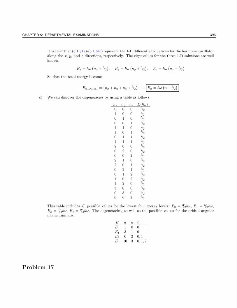
CHAPTER 5: DEPARTMENTAL EXAMINATIONS 395
It is clear that (5.1.84a)-(5.1.84c) represent the 1-D differential equations for the harmonic oscillatoralong the x, y, and z directions, respectively. The eigenvalues for the three 1-D solutions are wellknown,
Ex = ~ω(nx + 1/2
), Ey = ~ω
(ny + 1/2
), Ez = ~ω
(nz + 1/2
)
So that the total energy becomes
Enx,ny,nz =(nx + ny + nz + 3/2
)−→ En = ~ω
(n+ 3/2
)
c) We can discover the degeneracies by using a table as follows
nx ny nz E(~ω)0 0 0 3/21 0 0 5/20 1 0 5/20 0 1 5/21 1 0 7/21 0 1 7/20 1 1 7/21 1 1 9/22 0 0 7/20 2 0 7/20 0 2 7/22 1 0 9/22 0 1 9/20 2 1 9/20 1 2 9/21 0 2 9/21 2 0 9/23 0 0 9/20 3 0 9/20 0 3 9/2
This table includes all possible values for the lowest four energy levels: E0 = 3/2~ω, E1 = 5/2~ω,E2 = 7/2~ω, E3 = 9/2~ω. The degeneracies, as well as the possible values for the orbital angularmomentum are:
E d n `
E0 1 0 0E1 3 1 0E2 6 2 0, 1E3 10 3 0, 1, 2
Problem 17
W. Erbsen QUANTUM MECHANICS
a) Consider a helium ion. The two electrons are in the 2p and 3p states. The energy levels will have definite totalangular momentum (J = L + S). What J-values can occur and how many degenerate energy levels for each Jcan there be?
b) How do your answers change if the electrons are both in the 3p states?
Solution
a) Let’s call the electron in the 2p state “1”, and the electron in the 3p state “2.” Then `1 = 1, and`2 = 1. The total orbital angular momentum can then take the values
L = |`1 − `2|, ..., |`1 + `2| = 0, 1, 2 (5.1.85)
And for electrons, ms = ±1/2, so the possible values for the total spin angular momentum are
S = 0, 1 (5.1.86)
And we also know that the possible values for the total angular momentum is determined by
J = L+ S = |L− S|, ..., |L+ S| (5.1.87)
And to find the possible values, we create a table:
L S J0 1 11 1 0, 1, 22 1 1, 2, 30 0 01 0 12 0 2
So, the possible values for J are J = 0, 1, 2, 3 , each with degeneracies 2J + 1:
J D
0 11 32 53 7
b) If both electrons are in the 3p state, then
L = 0, 1, 2S = 0
And the possible total angular momentum quantum numbers can be found by
L S J
0 0 01 0 12 0 2
So the possible values for J are J = 0, 1, 2 . The degeneracies are
CHAPTER 5: DEPARTMENTAL EXAMINATIONS 397
J D0 11 32 5
Problem 18
A particle of spin zero is confined in a two-dimensional infinite square well of dimension 2a on each side.
a) Find the energies and the wave functions of the first two states.
b) If there are two indistinguishable noninteracting spin 1/2 particles inside the box, write down the total wavefunction of the first two states. Identify the degree of degeneray for each state.
c) If there are five indistinguishable spin 1/2 noninteracting particles in the box, what is the total energy of theground state?
d) If there are five indistinguishable spin 1 noninteracting particles in the box, what is the total energy of theground state?
Solution
a) In general, the eigenstates and energy eigenvalues for this problem are given by
ψ(x, y) =1
asin(nxπx
2a
)sin(nyπy
2a
)(5.1.88a)
Enx,ny =π2~2
8ma2(n2
x + nxy) = E0(n
2x + n2
y) (5.1.88b)
The the ground state, nx = ny = 1, (5.1.88a) and (5.1.88b) become
ψ(x, y) =1
asin(πx
2a
)sin(πy
2a
), E11 = 2E0
For the first excited state, nx = 2, and ny = 1, so we have
ψ(x, y) =1
asin(πxa
)sin(πy
2a
), E12 = 5E0
So, the first excited state is doubly degenerate.
b) We first recall that the total wave function of a fermion (space and spin part) must be completelyanti-symmetric under the exchange of any two particles in the system.
For the case at hand, we may have to “symmetrize,” or “anti-symmetrize” the wave functionsuch that the final total wave function is anti-symmetric. In other words, if the spin part is sym-metric, then the space part must be anti-symmetric, and also vice versa.
We recall that, in general,
W. Erbsen QUANTUM MECHANICS
ψ(x1, x2) =1√2
[ψn1(x1)ψn2(x2) ± ψn2(x1)ψn1(x2)] (5.1.89)
And also
ψ(x1, x2) =1
asin(n1πx1
2a
)sin(n2πx2
2a
)(5.1.90)
For the ground state, n1 = n2 = 1 and S = 0 (singlet) so the space part is just
ψ(x1, x2) =1
asin(πx1
2a
)sin(πx2
2a
)(5.1.91)
Since the space part is symmetric, the spin part must be anti-symmetric:
χ00 =
1√2
[|↑↓〉 − |↓↑〉] (5.1.92)
The total wave function for the ground state for two indistinguishable spin-1/2 fermions is just theproduct of (5.1.91) and (5.1.92)
ψ(x1, x2) =1
a√
2sin(πx1
2a
)sin(πx2
2a
)[|↑↓〉 − |↓↑〉]
The ground state has singlet degeneracy. For the first excited state, where are two different options:electron 1 can be excited or electron 2 can be excited.
Either of the first excited states may have by a symmetric (S = 0) or an anti-symmetric (S = 1)spatial wave function, like (5.1.89). In our case, letting n1 = 1 and n2 = 2,
ψ(x1, x2) =1
a√
2
[sin(πx1
2a
)sin(πx2
a
)+ sin
(πx1
a
)sin(πx2
2a
)](5.1.93a)
=1
a√
2
[sin(πx1
2a
)sin(πx2
a
)− sin
(πx1
a
)sin(πx2
2a
)](5.1.93b)
Where (5.1.93a) is symmetric and thus has an anti-symmetric spin part, while (5.1.93b) is anti-symmetric , and must have a symmetric spin part. The former is familiar; the latter (S = 1) hasthree components, each corresponding to one of the available symmetric spin functions. So, thisgives us four wave functions:
ψ(x1, x2) =1
a√
2
[sin(πx1
2a
)sin(πx2
a
)+ sin
(πx1
a
)sin(πx2
2a
)] 1√2
[|↑↓〉 − |↓↑〉]
=1
a√
2
[sin(πx1
2a
)sin(πx2
a
)− sin
(πx1
a
)sin(πx2
2a
)]|↑↑〉
=1
a√
2
[sin(πx1
2a
)sin(πx2
a
)− sin
(πx1
a
)sin(πx2
2a
)] 1√2
[|↑↓〉+ |↓↑〉]
=1
a√
2
[sin(πx1
2a
)sin(πx2
a
)− sin
(πx1
a
)sin(πx2
2a
)]|↓↓〉
We arrive at four more wave functions if we choose n1 = 2 and n2 = 1. Therefore, the first excitedstate is eightfold degenerate, and
E = 5E0
CHAPTER 5: DEPARTMENTAL EXAMINATIONS 399
c) If there are five indistinguishable spin 1/2 fermions in the box, the total energy of the ground statecan be determined via a table:
n1 n2 E d1 1 2E0 11 2 5E0 42 1 5E0 4
There can be two electrons per each set of quantum numbers, so we can fit five in the first two rows,so
E = 2 · 2E0 + 3 · 5E0 −→ E = 19E0
d) For five indistinguishable spin-1 bosons, all the particles can be in the lowest level, so the groundstate is just
E = 5 · 2E0 −→ E = 10E0
Problem 19
Ten electrons are confined in a box of dimensions (a, 2a, 2a) on each side. Calculate the total energy of theground state of these ten electrons if we assume that the electrons do not interact with each other.
Solution
The separated eigenfunctions and associated eigenenergies are
ψ(x) =
√2
asin(nxπx
a
), Ex =
n2xπ
2~2
2ma2(5.1.94a)
ψ(y) =
√1
asin(nyπy
2a
), Ey =
n2yπ
2~2
8ma2(5.1.94b)
ψ(z) =
√1
asin(nzπz
2a
), Ez =
n2zπ
2~2
8ma2(5.1.94c)
The total energy is thenEnxnynz =
π2~2
8ma2
(4n2
x + n2y + n2
z
)(5.1.95)
In order to find out which combination of atomic numbers yield the ground state, we create a table:

W. Erbsen QUANTUM MECHANICS
nx ny nz 4n2x n2
y n2z Σ #
1 1 1 4 1 1 6 11 1 2 4 1 4 9 21 2 1 4 4 1 9 32 1 1 16 1 1 182 1 2 16 1 4 212 2 1 16 4 1 211 2 2 4 4 4 12 41 1 3 4 1 9 14 51 3 1 4 9 1 153 1 1 36 1 1 38
With fermions, two can have each energy (±1/2), so we picked the five lowest energies and now multiplythem by two and sum to find the total ground state energy:
E =π2~2
8ma2[2 (6 + 9 + 9 + 12 + 14)] −→ E =
100π2~2
8ma2
Problem 23
Suppose a particle moves in one dimension under the potential V (x). V (x) is even, that is V (x) = V (−x).Also, all the eigenstates of the Hamiltonian H are known to be non-degenerate.
a) Prove that every eigenstate of H has either even or odd parity.
b) Consider a completely free particle in one dimension. Show that there are solutions to the eigenvalue equationwhich do not have well-defined parity. Explain why this is not a contradiction to the theorem of part (a).
Solution
a) To show that every eigenstate of H has either even or odd parity, we apply the parity operator tothe time-independent Schrodinger equation:
PHψ(x) =P
(p2
2m+ V (x)
)ψ(x) =
(p2
2m+ V (−x)
)ψ(−x) =
(p2
2m+ V (x)
)ψ(−x) (5.1.96)
If we were to apply the parity operator twice,
P 2Hψ(x) = P
(p2
2m+ V (x)
)ψ(−x) =
(p2
2m+ V (x)
)ψ(x) (5.1.97)
So, we can see that P 2 has an eigenvalue of 1: P 2 = 1 −→ P = ±1. Furthermore, P and Hcommute, so they must share the same eigenvector. Since the eigenstates of P can have either evenor odd parity (p = ±1), and H and P commute (have same eigenvector), then every eigenstate ofH must have either even or odd parity.
CHAPTER 5: DEPARTMENTAL EXAMINATIONS 401
b) A free particle is described by
ψ+(x) = Aeikx, ψ−(x) = Ae−ikx
And if we apply the parity operator once,
Pψ+(x) =PAeikx = Ae−ikx
Pψ−(x) =PAe−ikx = Aeikx
Since ψ+(x) and ψ−(x) have the same energy (they are degenerate), we cannot follow the samelogic as in a).
Problem 24
Consider an isotropic 3D spherical square well. What are the conditions on the depth V0 and radius a suchthat a particle of mass m has exactly one bound state in this well? Show your reasoning and calculations.
Solution
The radial equation that we wish to solve is in terms of a intermediary function U(r) = rR(r) One couldjust imagine it to be ψ and carry on, since it plays no important part here.
(− ~2
2m
∂
∂r2+ V +
~2
2m
`(` + 1)
r2
)U(r) = EU(r) (5.1.98)
However, for the ground state, we recognize that ` = 0 and Veff → V , and (5.1.98) becomes
(− ~2
2m
∂
∂r2+ V
)U(r) = EU(r) (5.1.99)
For our isotropic spherical square well, we define two regions; I is inside the sphere, where V = −V0,and II is outside, where V = 0. Our task is to first solve (5.1.99) for each of these two regions. Startingwith region I,
(− ~2
2m
∂
∂r2− V0
)U(r) = EU(r)
∂2
∂r2u(r) +
2m(E + V0)
~2U(r) = 0
∂2
∂r2U(r) + k2U(r) = 0, k =
√2m(E + V0)
~(5.1.100)
The solution of (5.1.100) is
UI (r) = A sin (kr) + B cos (kr) (5.1.101)
And now for region II,
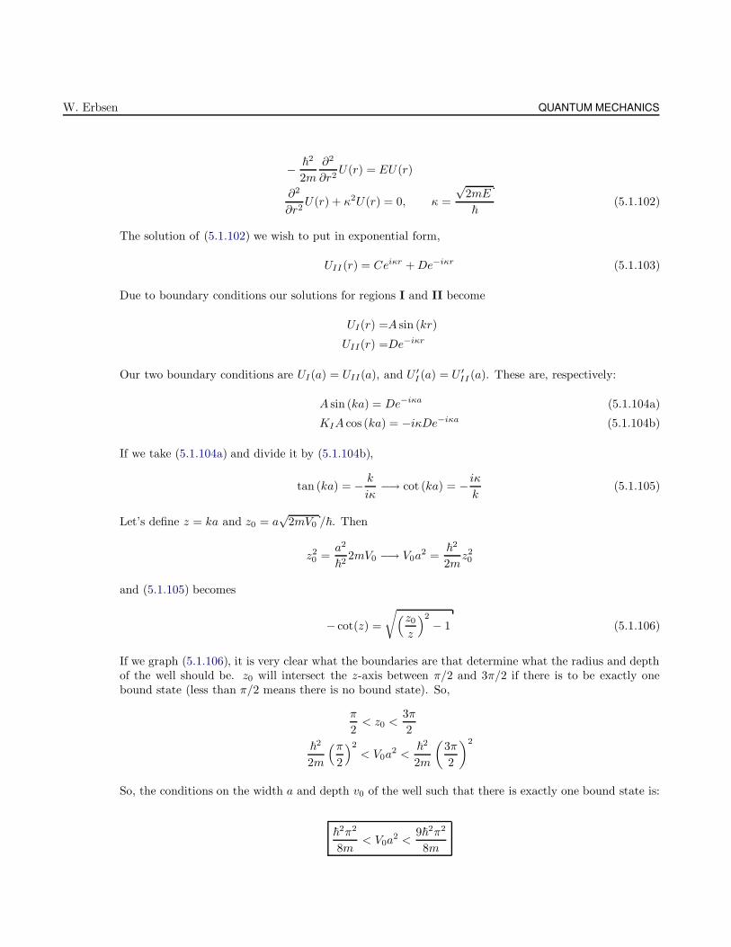
W. Erbsen QUANTUM MECHANICS
− ~2
2m
∂2
∂r2U(r) = EU(r)
∂2
∂r2U(r) + κ2U(r) = 0, κ =
√2mE
~(5.1.102)
The solution of (5.1.102) we wish to put in exponential form,
UII (r) = Ceiκr +De−iκr (5.1.103)
Due to boundary conditions our solutions for regions I and II become
UI(r) =A sin (kr)
UII(r) =De−iκr
Our two boundary conditions are UI(a) = UII(a), and U ′I (a) = U ′
II (a). These are, respectively:
A sin (ka) = De−iκa (5.1.104a)
KIA cos (ka) = −iκDe−iκa (5.1.104b)
If we take (5.1.104a) and divide it by (5.1.104b),
tan (ka) = − k
iκ−→ cot (ka) = − iκ
k(5.1.105)
Let’s define z = ka and z0 = a√
2mV0 /~. Then
z20 =
a2
~22mV0 −→ V0a
2 =~2
2mz20
and (5.1.105) becomes
− cot(z) =
√(z0z
)2
− 1 (5.1.106)
If we graph (5.1.106), it is very clear what the boundaries are that determine what the radius and depthof the well should be. z0 will intersect the z-axis between π/2 and 3π/2 if there is to be exactly onebound state (less than π/2 means there is no bound state). So,
π
2< z0 <
3π
2
~2
2m
(π2
)2
< V0a2 <
~2
2m
(3π
2
)2
So, the conditions on the width a and depth v0 of the well such that there is exactly one bound state is:
~2π2
8m< V0a
2 <9~2π2
8m
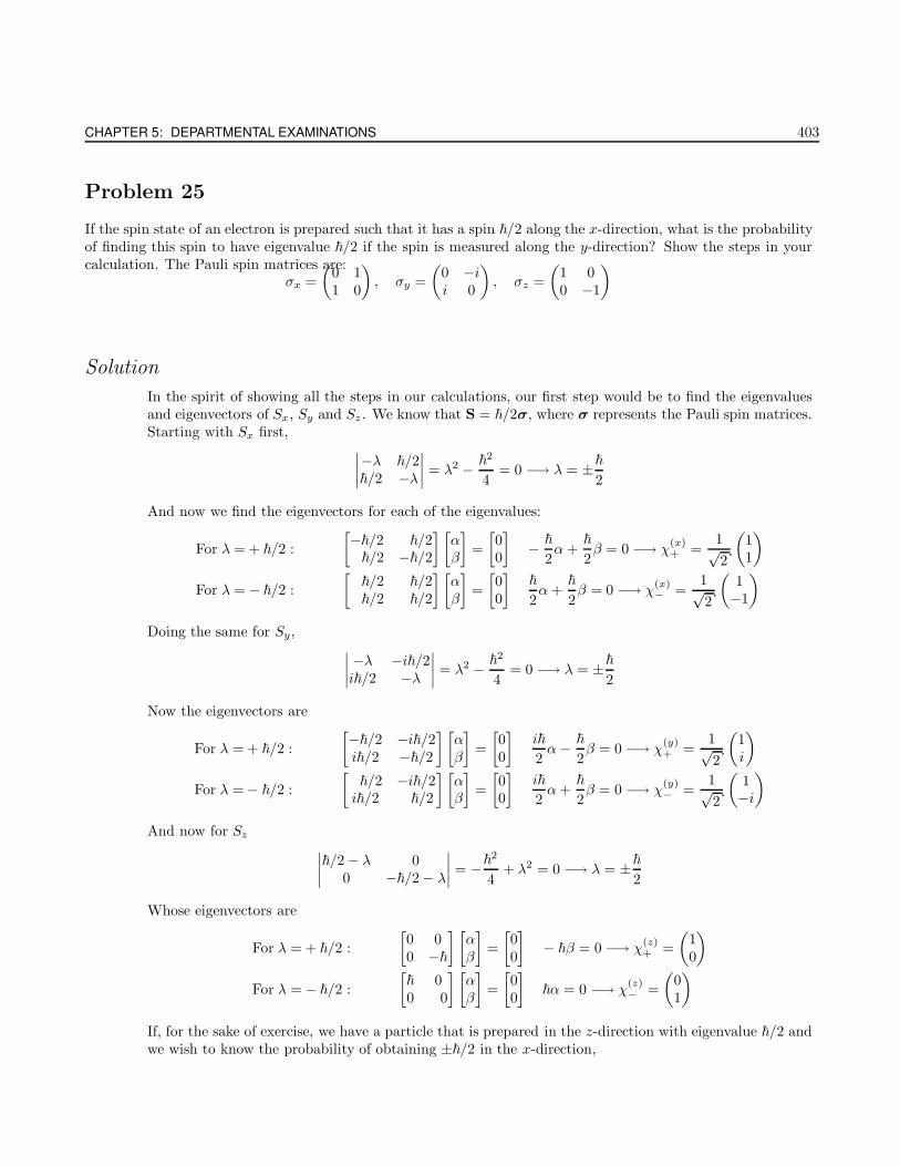
CHAPTER 5: DEPARTMENTAL EXAMINATIONS 403
Problem 25
If the spin state of an electron is prepared such that it has a spin ~/2 along the x-direction, what is the probabilityof finding this spin to have eigenvalue ~/2 if the spin is measured along the y-direction? Show the steps in yourcalculation. The Pauli spin matrices are:
σx =
(0 11 0
), σy =
(0 −ii 0
), σz =
(1 00 −1
)
Solution
In the spirit of showing all the steps in our calculations, our first step would be to find the eigenvaluesand eigenvectors of Sx, Sy and Sz . We know that S = ~/2σ, where σ represents the Pauli spin matrices.Starting with Sx first,
∣∣∣∣−λ ~/2~/2 −λ
∣∣∣∣ = λ2 − ~2
4= 0 −→ λ = ±~
2
And now we find the eigenvectors for each of the eigenvalues:
For λ = + ~/2 :
[−~/2 ~/2
~/2 −~/2
] [αβ
]=
[00
]− ~
2α+
~
2β = 0 −→ χ
(x)+ =
1√2
(11
)
For λ = − ~/2 :
[~/2 ~/2~/2 ~/2
] [αβ
]=
[00
]~
2α+
~
2β = 0 −→ χ
(x)− =
1√2
(1−1
)
Doing the same for Sy,∣∣∣∣−λ −i~/2i~/2 −λ
∣∣∣∣ = λ2 − ~2
4= 0 −→ λ = ±~
2
Now the eigenvectors are
For λ = + ~/2 :
[−~/2 −i~/2i~/2 −~/2
] [αβ
]=
[00
]i~
2α− ~
2β = 0 −→ χ
(y)+ =
1√2
(1i
)
For λ = − ~/2 :
[~/2 −i~/2i~/2 ~/2
] [αβ
]=
[00
]i~
2α+
~
2β = 0 −→ χ
(y)− =
1√2
(1−i
)
And now for Sz
∣∣∣∣~/2 − λ 0
0 −~/2 − λ
∣∣∣∣ = −~2
4+ λ2 = 0 −→ λ = ±~
2
Whose eigenvectors are
For λ = + ~/2 :
[0 00 −~
] [αβ
]=
[00
]− ~β = 0 −→ χ
(z)+ =
(10
)
For λ = − ~/2 :
[~ 00 0
] [αβ
]=
[00
]~α = 0 −→ χ
(z)− =
(01
)
If, for the sake of exercise, we have a particle that is prepared in the z-direction with eigenvalue ~/2 andwe wish to know the probability of obtaining ±~/2 in the x-direction,
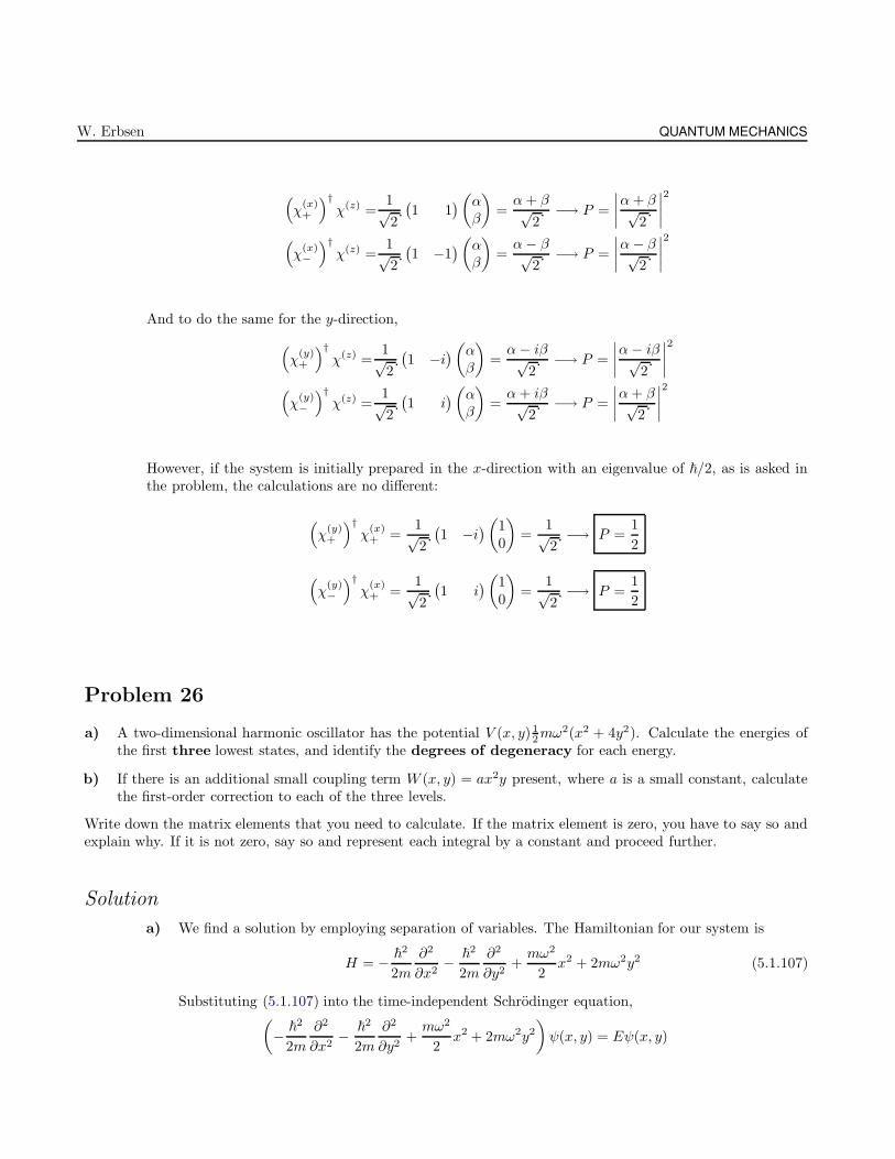
W. Erbsen QUANTUM MECHANICS
(χ
(x)+
)†χ(z) =
1√2
(1 1
)(αβ
)=α+ β√
2−→ P =
∣∣∣∣α+ β√
2
∣∣∣∣2
(χ
(x)−
)†χ(z) =
1√2
(1 −1
)(αβ
)=α− β√
2−→ P =
∣∣∣∣α− β√
2
∣∣∣∣2
And to do the same for the y-direction,
(χ
(y)+
)†χ(z) =
1√2
(1 −i
)(αβ
)=α− iβ√
2−→ P =
∣∣∣∣α− iβ√
2
∣∣∣∣2
(χ
(y)−
)†χ(z) =
1√2
(1 i
)(αβ
)=α+ iβ√
2−→ P =
∣∣∣∣α+ β√
2
∣∣∣∣2
However, if the system is initially prepared in the x-direction with an eigenvalue of ~/2, as is asked inthe problem, the calculations are no different:
(χ
(y)+
)†χ
(x)+ =
1√2
(1 −i
)(10
)=
1√2
−→ P =1
2
(χ
(y)−
)†χ
(x)+ =
1√2
(1 i
)(10
)=
1√2
−→ P =1
2
Problem 26
a) A two-dimensional harmonic oscillator has the potential V (x, y)12mω
2(x2 + 4y2). Calculate the energies ofthe first three lowest states, and identify the degrees of degeneracy for each energy.
b) If there is an additional small coupling term W (x, y) = ax2y present, where a is a small constant, calculatethe first-order correction to each of the three levels.
Write down the matrix elements that you need to calculate. If the matrix element is zero, you have to say so andexplain why. If it is not zero, say so and represent each integral by a constant and proceed further.
Solution
a) We find a solution by employing separation of variables. The Hamiltonian for our system is
H = − ~2
2m
∂2
∂x2− ~2
2m
∂2
∂y2+mω2
2x2 + 2mω2y2 (5.1.107)
Substituting (5.1.107) into the time-independent Schrodinger equation,(− ~2
2m
∂2
∂x2− ~2
2m
∂2
∂y2+mω2
2x2 + 2mω2y2
)ψ(x, y) = Eψ(x, y)
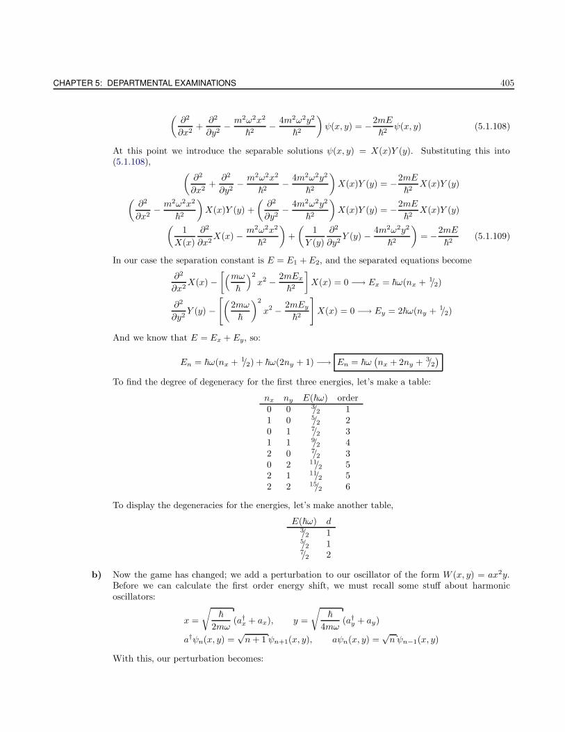
CHAPTER 5: DEPARTMENTAL EXAMINATIONS 405
(∂2
∂x2+
∂2
∂y2− m2ω2x2
~2− 4m2ω2y2
~2
)ψ(x, y) = −2mE
~2ψ(x, y) (5.1.108)
At this point we introduce the separable solutions ψ(x, y) = X(x)Y (y). Substituting this into(5.1.108),
(∂2
∂x2+
∂2
∂y2− m2ω2x2
~2− 4m2ω2y2
~2
)X(x)Y (y) = −2mE
~2X(x)Y (y)
(∂2
∂x2− m2ω2x2
~2
)X(x)Y (y) +
(∂2
∂y2− 4m2ω2y2
~2
)X(x)Y (y) = −2mE
~2X(x)Y (y)
(1
X(x)
∂2
∂x2X(x) − m2ω2x2
~2
)+
(1
Y (y)
∂2
∂y2Y (y) − 4m2ω2y2
~2
)= −2mE
~2(5.1.109)
In our case the separation constant is E = E1 +E2, and the separated equations become
∂2
∂x2X(x) −
[(mω~
)2
x2 − 2mEx
~2
]X(x) = 0 −→ Ex = ~ω(nx + 1/2)
∂2
∂y2Y (y) −
[(2mω
~
)2
x2 − 2mEy
~2
]X(x) = 0 −→ Ey = 2~ω(ny + 1/2)
And we know that E = Ex + Ey, so:
En = ~ω(nx + 1/2) + ~ω(2ny + 1) −→ En = ~ω(nx + 2ny + 3/2
)
To find the degree of degeneracy for the first three energies, let’s make a table:
nx ny E(~ω) order0 0 3/2 11 0 5/2 20 1 7/2 31 1 9/2 42 0 7/2 30 2 11/2 52 1 11/2 52 2 15/2 6
To display the degeneracies for the energies, let’s make another table,
E(~ω) d3/2 15/2 17/2 2
b) Now the game has changed; we add a perturbation to our oscillator of the form W (x, y) = ax2y.Before we can calculate the first order energy shift, we must recall some stuff about harmonicoscillators:
x =
√~
2mω(a†x + ax), y =
√~
4mω(a†y + ay)
a†ψn(x, y) =√n+ 1 ψn+1(x, y), aψn(x, y) =
√n ψn−1(x, y)
With this, our perturbation becomes:

W. Erbsen QUANTUM MECHANICS
W =a
(√~
2mω(a†x + ax)
)2(√~
4mω(a†y + ay)
)
=a~
2mω
√~
4mω(a†x + ax)2(a†y + ay) (5.1.110)
In general, the first order shift in energy is given by
E(1)n =〈nx|〈ny|W (x, y)|ny〉|nx〉
=a~
2mω
√~
4mω〈nx|〈ny|(a†x + ax)2(a†y + ay)|ny〉|nx〉
=a~
2mω
√~
4mω
[〈nx|〈ny|(a†x + ax)2a†y|ny〉|nx〉 + 〈nx| 〈ny|(a†x + ax)2ay|ny〉|nx〉
]
=a~
2mω
√~
4mω
[√ny + 1 〈nx|〈ny|(a†x + ax)2|ny + 1〉|nx〉 +
√ny 〈nx|〈ny|(a†x + ax)2|ny − 1〉|nx〉
]
(5.1.111)
Problem 28
A particle is in the ground state of an infinite square well. That is
V (x) =
0 0 ≤ x ≤ L∞ otherwise
(5.1.112)
At t = 0 the wall at x = L is suddenly moved to x = 2L - this happens very fast, approximately instantaneously.
a) Calculate the probability that long after t = 0 the system is in the ground state of the new potential.
b) How fast must the change take place for this “instantaneous” assumption to be good?
Solution
The eigenstates for the ground states before and arbitrary eigenstates after the transition are
ψgs(x) =
√2
Lsin(πxL
)(5.1.113a)
ψn(x) =
√1
Lsin(nπx
2L
)(5.1.113b)
a) We wish to express our initial ground state wave function ψgs(x) in terms of a linear combinationof ψn(x) states:
ψgs =
√2
Lsin(πxL
)=∑
n
cnψn(x) =
√1
L
∑
n
cn sin(nπx
2L
)
For the probability that we will be in the ground state, we calculate cn for n = 1:
CHAPTER 5: DEPARTMENTAL EXAMINATIONS 407
cn =
∫ L
0
ψgs(x)ψn(x) dx
=
√2
L
∫ L
0
sin(πxL
)sin(πx
2L
)dx
=
√2
L
∫ L
0
1
2
[cos(πxL
− πx
2L
)− cos
(πxL
+πx
2L
)]dx
=
√2
L
1
2
∫ L
0
[cos(πx
2L
)− cos
(3πx
2L
)]dx
=
√2
2L
[2L
πsin(πx
2L
)− 2L
3πsin
(3πx
2L
)∣∣∣∣L
0
=
√2
2L
[2L
πsin(π
2
)− 2L
3πsin
(3π
2
)]
=
√2
2L
[2L
π+
2L
3π
]
=4√
2
3π
So, the probability that we will remain in the ground state is
|c1|2 =32
9π2
b) To find out how fast this process must take place, we use the time-energy uncertainty relation:∆t∆E ∝ ~. We find the change in energy first
∆E =n2π2~2
8mL2− n2π2~2
2mL2=
3n2π2~2
8mL2
So, the necessary time is (approximately)
∆t =8mL2
3n2π2~
Problem 29
The scattering amplitude for a proton on a target atom is f(θ). That is, if the target is at rT = 0 then farfrom the target the wavefunction is
ψ(r) = eik·r + f(θ)eikr
r(5.1.114)
a) Suppose that there are N(N 1) target atoms located at the point r1 = A, r2 = 2A, r3 = 3A and so on.What is ψ(r) for positions r far from the line? That is, find ψ(r) for |r| N |A|. It will have the form
ψ(r) = eik·r + F (θ)eikr
r(5.1.115)
Find F (θ) and dσ/dΩ = |F (θ)|2. Is dσ/dΩ ∼ N?
W. Erbsen QUANTUM MECHANICS
b) Suppose now that the N(N 1) target atoms are located at random positions, but all inside a small finiteball of radius R. Calculate F (θ) and dσ/dΩ. Is dσ/dΩ ∼ N?
Solution
a) For some point P very far from the target, then we can make the approximation that r1 ≈ r2 ≈r3 ≈ r. We start with the template provided, (5.1.115), but add to it an additional phase term:
ψ(r) =eikr + f(θ)
N∑
n=0
eikr−inkA
r
=eikr +eikr
rf(θ)
N∑
n=0
e−inkA (5.1.116)
The sum in (5.1.117) is finite; to evaluate it, we let∑e−inkr =
∑an, where a = e−ikr. Then
N∑
n=0
an = 1 + a+ a2 + a3 + ...+ aN−1
1+
N∑
n=0
an+1 = 1 + a+ a2 + a3 + ...+ aN−1 + aN
1+
N∑
n=0
an+1 =
N∑
n=0
an + aN
1 − aN =
N∑
n=0
an −N∑
n=0
an+1
1 − aN =
N∑
n=0
an(1 − a)
N∑
n=0
an =1 − aN
1 − a
Using this, (5.1.117) becomes
ψ(r) = eikr +eikr
r
[1 − e−iNkr
1 − e−ikr
]f(θ) (5.1.117)
From (5.1.117), it is clear that F (θ) is simply the term in the brackets,
F (θ) =1 − e−iNkr
1 − e−ikrf(θ)
And now to find the differential cross section,
dσ
dΩ= |F (θ)|2
CHAPTER 5: DEPARTMENTAL EXAMINATIONS 409
=
∣∣∣∣1 − e−iNkr
1 − e−ikrf(θ)
∣∣∣∣2
=
∣∣∣∣e−iNkr/2
e−ikr/2
(eiNkr/2 − e−iNkr/2
eikr/2 − e−ikr/2
))
∣∣∣∣2
|f(θ)|2
=
∣∣∣∣e−iNkr
e−ikr
sin (Nkr/2)
sin (kr/2)
∣∣∣∣2
|f(θ)|2
From which it is clear that
dσ
dΩ=
sin2 (Nkr/2)
sin2 (kr/2)|f(θ)|2
No, the differential cross section is not proportional to N .
b) For the case of gathered target atoms we start in much the same way,
ψ(r) =eikr + f(θ)
N∑
n=0
eikr−iXnk
r
=eikr +eikr−iXnk
rf(θ)
N∑
n=0
e−iXnk (5.1.118)
Where Xn represents the displacement of the nth target particle. From (5.1.118) it is clear that
F (θ) = f(θ)
N∑
n=0
e−iXnk (5.1.119)
To find the differential cross section,
dσ
dΩ= |F (θ)|2
=
∣∣∣∣∣f(θ)N∑
n=0
e−iXnk
∣∣∣∣∣
2
= |f(θ)|2(
N∑
n=0
eiXnk
)(N∑
m=0
e−iXmk
)
= |f(θ)|2N∑
n=0m=0
eik(Xn−Xm)
= |f(θ)|2
N∑
n=m=1
eik(Xn−Xm) +
N∑
n 6=m=1
eik(Xn−Xm)
= |f(θ)|2
N∑
n=m=1
e0 +
N∑
n 6=m=1
eik(Xn−Xm)
W. Erbsen ELECTRODYNAMICS
= |f(θ)|2N +
N∑
n 6=m=1
eik(Xn−Xm)
(5.1.120)
The remaining sum is often referred to as random walk, where the trajectories are completely randomand as an ensemble, average to zero. Thus, our differential cross section is
dσ
dΩ= N |f(θ)|2
There is no escaping the fact that the differential cross section is proportional to the number ofatoms in this particular configuration.
5.2 Electrodynamics
Problem 1
A conducting sphere of radius a is placed in a uniform electrostatic field E0. If the sphere is well insulated,find the expressions for potential and electric fields V and E at the point P (r, θ, φ) lying outside the sphere. Alsoobtain the expression for the induced surface charge density σ and show that it forms a dipole distribution. Specifiyyour boundary conditions clearly.
Solution
The induced surface charge density is σ(θ) = ε0E; the plan of action then is to calculate E, which canbe readily done by intermediately solving for the potential, V :
V (r, θ) =
∞∑
`=0
(A`r
` +B`
r`+1
)P` (cos θ) (5.2.1)
Where (5.2.1) stems from (3.63) in Griffiths. The problem, then, is to take (5.2.1) and adjust it so thatit describes our problem. We do this by applying boundary conditions. It should be mentioned thatas a conductor, the sphere has a constant potential, but we are only interested in the potential outsideof the sphere, so we can choose it to be whatever we want. The most convenient choice would be tolet Vsphere = 0. Additionally, we recognize that in the field (absent from the sphere) the potential isV (r, θ) = −E0r cos θ. We can now form our boundary conditions:
V (r, θ) =
0 at r = R−E0r cos θ at r → ∞
Applying our first boundary condition to (5.2.1),
V (R, θ) =
∞∑
`=0
(A`R
` +B`
R`+1
)P` (cos θ) = 0 −→ A`R
` +B`
R`+1= 0 −→ B` = −A`R
2`+1 (5.2.2)

CHAPTER 5: DEPARTMENTAL EXAMINATIONS 411
Substituting our new value for B` into (5.2.1), we have
V (r, θ) =
∞∑
`=0
(A`r
` −A`R2`+1
r`+1
)P` (cos θ) (5.2.3)
If we apply the second boundary condition to (5.2.3), we find that the second term in parenthesisapproaches 0 as r → ∞, and we are left with
V (r, θ) =
∞∑
`=0
(A`r
`)P` (cos θ) = −E0r cos θ (5.2.4)
From (5.2.4) we can see that the second boundary condition is satisfied only if ` = 1 and A` = A1 = −E0.With these modifications, (5.2.3) is now
V (r, θ) =
(−E0r + E0
R3
r2
)cos θ (5.2.5)
From the potential, we can now find E, and in turn σ:
σ(θ) = − ε0∂
∂rV (r, θ)
= − ε0∂
∂r
[(−E0r − E0
R3
r2
)cos θ
]
= − ε0
[(−E0 − 2E0
R3
r3
)cos θ
∣∣∣∣r=R
From this it is easy to see that
σ(θ) = 3E0ε0 cos θ
Problem 2
Two insulated square parallel conducting plates, of side L and separation d, are charged with surface densi-ties +σ on the upper plate and −σ on the lower. Two dieletric slabs, each with thickness d/2 and area L × L,are inserted between the plates, one slab above the other. The dieletric constants are K1 and K2. Assume thatd L. Determine:
a) D everywhere between the plates.
b) E everywhere between the plates.
c) The bound surface charge densities σb on the three dialetric surfaces.
d) The capacitance.
Solution

W. Erbsen ELECTRODYNAMICS
a) We first recall that Gauss’ Law for for dielectrics can be written as∮
D · dA = Q
Where D = ε0KE is the electric displacement. In the current case, the area is just L ·L = L2, andthe surface charge density defines the total charge as Q = σL2, so that we have
DL2 = σL2 −→ D = −σ z for − d/2 < z < d/2 (5.2.6)
b) We again use the fact that D = ε0KE, such that Gauss’ Law becomes:
ε0K1,2EL2 = −σL2 z −→ E = − σ
ε0K1,2z (5.2.7)
And we now have
E =
− σ
ε0K1z for 0 < z < d/2
σ
ε0K2(−z) for −d/2 < z < 0
c) The bound surface charge density is related to the polarization as σb = P · n, where we rememberthat P = ε0χE. We also recall that the dielectric constant is defined as K = (1 +χ). The (general)polarization is then given by
|P1,2| = ε0χ1,2|E1,2| = ε0 (K1,2 − 1)E = ε0 (K1,2 − 1)
(σ
ε0K1,2
)=
(1 − 1
K1,2
)σ (5.2.8)
The three surfaces the prompt is speaking about refers to the top surface, where slab 1 interfaceswith the positive conducting plate (and analogously for slab 2 on the lower negative conductingplate), and the interface between the two dielectrics. The only tricky bit is in the interstitial region;but all we have to do is add the bound charge densities being contributed from both slabs. Theresult is
σb =
−(
1 − 1
K1
)σ for surface 1
(1 − 1
K1
)σ −
(1 − 1
K2
)σ for surface 2
(1 − 1
K2
)σ for surface 3
d) In order to calculate the capacitance, we first recall the relation Q = C|∆V |. So, it seems like all wewould have to do is calculate ∆V and we are home-free. We must integrate over both dielectrics,going from the negative terminal at the bottom of slab 2 to the positive terminal at the top of slab1:
∆V = −∫ 0
−d/2
E2 dz −∫ d/2
0
E1 dz
= −(− σ
ε0K2
)∫ 0
−d/2
dz −(− σ
ε0K1
)∫ d/2
0
dz
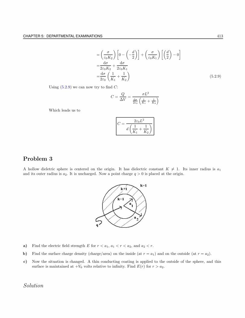
CHAPTER 5: DEPARTMENTAL EXAMINATIONS 413
=
(σ
ε0K2
)[0 −
(−d
2
)]+
(σ
ε0K1
)[(d
2
)− 0
]
=dσ
2ε0K2+
dσ
2ε0K1
=dσ
2ε0
(1
K1+
1
K2
)(5.2.9)
Using (5.2.9) we can now try to find C:
C =Q
∆V=
σL2
dσ2ε0
(1
K1+ 1
K2
)
Which leads us to
C =2ε0L
2
d
(1
K1+
1
K2
)
Problem 3
A hollow dieletric sphere is centered on the origin. It has dielectric constant K 6= 1. Its inner radius is a1
and its outer radius is a2. It is uncharged. Now a point charge q > 0 is placed at the origin.
a) Find the electric field strength E for r < a1, a1 < r < a2, and a2 < r.
b) Find the surface charge density (charge/area) on the inside (at r = a1) and on the outside (at r = a2).
c) Now the situation is changed. A thin conducting coating is applied to the outside of the sphere, and thissurface is maintained at +V0 volts relative to infinity. Find E(r) for r > a2.
Solution
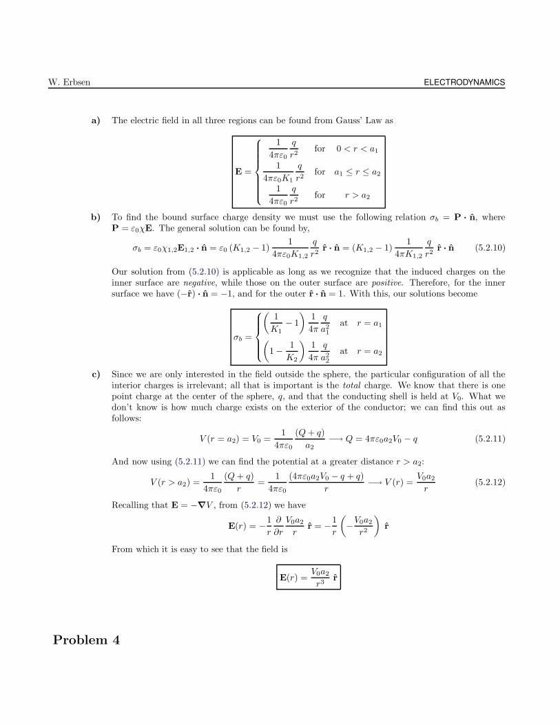
W. Erbsen ELECTRODYNAMICS
a) The electric field in all three regions can be found from Gauss’ Law as
E =
1
4πε0
q
r2for 0 < r < a1
1
4πε0K1
q
r2for a1 ≤ r ≤ a2
1
4πε0
q
r2for r > a2
b) To find the bound surface charge density we must use the following relation σb = P · n, whereP = ε0χE. The general solution can be found by,
σb = ε0χ1,2E1,2 · n = ε0 (K1,2 − 1)1
4πε0K1,2
q
r2r · n = (K1,2 − 1)
1
4πK1,2
q
r2r · n (5.2.10)
Our solution from (5.2.10) is applicable as long as we recognize that the induced charges on theinner surface are negative, while those on the outer surface are positive. Therefore, for the innersurface we have (−r) · n = −1, and for the outer r · n = 1. With this, our solutions become
σb =
(1
K1− 1
)1
4π
q
a21
at r = a1
(1 − 1
K2
)1
4π
q
a22
at r = a2
c) Since we are only interested in the field outside the sphere, the particular configuration of all theinterior charges is irrelevant; all that is important is the total charge. We know that there is onepoint charge at the center of the sphere, q, and that the conducting shell is held at V0. What wedon’t know is how much charge exists on the exterior of the conductor; we can find this out asfollows:
V (r = a2) = V0 =1
4πε0
(Q+ q)
a2−→ Q = 4πε0a2V0 − q (5.2.11)
And now using (5.2.11) we can find the potential at a greater distance r > a2:
V (r > a2) =1
4πε0
(Q+ q)
r=
1
4πε0
(4πε0a2V0 − q + q)
r−→ V (r) =
V0a2
r(5.2.12)
Recalling that E = −∇V , from (5.2.12) we have
E(r) = −1
r
∂
∂r
V0a2
rr = −1
r
(−V0a2
r2
)r
From which it is easy to see that the field is
E(r) =V0a2
r3r
Problem 4
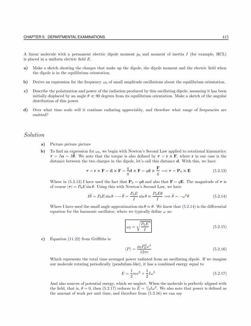
CHAPTER 5: DEPARTMENTAL EXAMINATIONS 415
A linear molecule with a permanent electric dipole moment p0 and moment of inertia I (for example, HCL)is placed in a uniform electric field E.
a) Make a sketch showing the charges that make up the dipole, the dipole moment and the electric field whenthe dipole is in the equilibrium orientation.
b) Derive an expression for the frequency ω0 of small amplitude oscillations about the equilibrium orientation.
c) Describe the polarization and power of the radiation produced by this oscillating dipole, assuming it has beeninitially displaced by an angle θ 90 degrees from its equilibrium orientation. Make a sketch of the angulardistribution of this power.
d) Over what time scale will it continue radiating appreciably, and therefore what range of frequencies areemitted?
Solution
a) Picture picture picture
b) To find an expression for ω0, we begin with Newton’s Second Law applied to rotational kinematics:τ = Iα = Iθ. We note that the torque is also defined by τ = r × F, where r in our case is thedistance between the two charges in the dipole, let’s call this distance d. With this, we have
τ = r × F = d × F =q
qd × F = qd ×
F
q=⇒ τ = P0 × E (5.2.13)
Where in (5.2.13) I have used the fact that P0 = qd and also that F = qE. The magnitude of τ isof course |τ | = P0E sin θ. Using this with Newton’s Second Law, we have
Iθ = P0E sin θ −→ θ =P0E
Isin θ ≈ P0Eθ
I=⇒ θ = −ω2θ (5.2.14)
Where I have used the small angle approximation sin θ ≈ θ. We know that (5.2.14) is the differentialequation for the harmonic oscillator, where we typically define ω as:
ω0 =
√P0E
I(5.2.15)
c) Equation (11.22) from Griffiths is:
〈P 〉 =µ0P
20ω
4
12πc(5.2.16)
Which represents the total time averaged power radiated from an oscillating dipole. If we imagineour molecule rotating periodically (pendulum-like), it has a combined energy equal to
E =1
2mv2 +
1
2Iω2 (5.2.17)
And also sources of potential energy, which we neglect. When the molecule is perfectly aligned withthe field, that is, θ = 0, then (5.2.17) reduces to E = 1/2Iω
2 . We also note that power is defined asthe amount of work per unit time, and therefore from (5.2.16) we can say
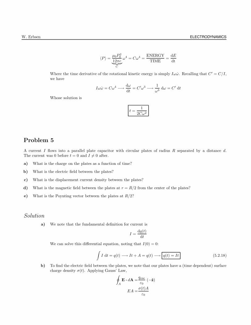
W. Erbsen ELECTRODYNAMICS
〈P 〉 =µ0P
20
12πc︸ ︷︷ ︸C
ω4 = Cω4 =ENERGY
TIME=
dE
dt
Where the time derivative of the rotational kinetic energy is simply Iωω. Recalling that C ′ = C/I,we have
Iωω = Cω4 −→ dω
dt= C ′ω3 −→ 1
ω3dω = C ′ dt
Whose solution is
t =1
2Cω2
Problem 5
A current I flows into a parallel plate capacitor with circular plates of radius R separated by a distance d.The current was 0 before t = 0 and I 6= 0 after.
a) What is the charge on the plates as a function of time?
b) What is the electric field between the plates?
c) What is the displacement current density between the plates?
d) What is the magnetic field between the plates at r = R/2 from the center of the plates?
e) What is the Poynting vector between the plates at R/2?
Solution
a) We note that the fundamental definition for current is
I =dq(t)
dt
We can solve this differential equation, noting that I(0) = 0:
∫I dt = q(t) −→ It +A = q(t) −→ q(t) = It (5.2.18)
b) To find the electric field between the plates, we note that our plates have a (time dependent) surfacecharge density σ(t). Applying Gauss’ Law,
∮
A
E · dA =qenc
ε0(−z)
EA =σ(t)A
ε0
CHAPTER 5: DEPARTMENTAL EXAMINATIONS 417
E =1
ε0
q(t)
πR2(−z) (5.2.19)
From (5.2.19) and using (5.2.18), the electric field is given by
E =It
ε0πR2(−z) (5.2.20)
c) We know that the displacement current density is denoted by Jd and is given by
Jd = ε0∂E
∂t+∂P
∂t(5.2.21)
The displacement current density is obtained simply by taking the time derivative of the electricdisplacement field D = ε0E+P. In our case, we have no dielectric media so the last term in (5.2.21)is neglected. Using (5.2.20), Jd becomes
Jd =∂
∂t
(It
ε0πR2(−z)
)
Which is simple enough to evaluate. The result is:
Jd =I
ε0πR2(−z) (5.2.22)
d) The magnetic field at a position r = R/2 between the plates can be computed using Ampere’s Law:∮
B · d` =µ0Ienc
In we are allowed to switch Ienc with Id since the magnetic field within the plates is the sameas between the plates. We also note that the displacement current density Jd is related to thedisplacement current Id by Jd = Id/πR
2 (in the following case R is actually r). So, with (5.2.22),(d) becomes:
B2πr =µ0Jdπr2
B2πr =µ0
(I
πR2(−z)
)πr2
B = − µ0Ir
2πR2z (5.2.23)
If we recall that r = R/2, it is easy to see that (5.2.23) can be written as:
B = − µ0I
4πRφ (5.2.24)
e) The fundamental formulation for the Poyinting Vector is
S =1
µ0E × B (5.2.25)
Inserting our previously tabulated values for E from (5.2.20) and B from (5.2.24), (5.2.25) becomes:
S =1
µ0
(− It
ε0πR2z
)×
(− µ0I
4πRφ
)
W. Erbsen ELECTRODYNAMICS
Which can be rewritten as
S =I2t
4ε0π2R3ρ
Problem 6
A sphere of radius R carries charge Q distributed uniformly over its surface. The sphere is rotated at a con-stant angular velocity ω around the z-axis. Calculate the magnetic dipole moment. Find the magnetic field at thepoint (x, 0, 0) where x R.
Solution
The integral form of the magnetic dipole moment is
µ =
∫I dA =
∫A dI (5.2.26)
We also recall that the definition of current is I = dQ/dt, but if we want the differential element of theamount of current over some specified length of time (the period, T ), this becomes dI = dQ/T . Thedifferential charge element in our case since we have a surface charge density is dQ = σ dA.
So, theoretically we just insert our values into (5.2.26) and integrate. we begin by looking for thecharge element dQ for a thin strip of the sphere, rotating around at some radius r = a sin θ with someangular velocity ω. This rotating charge, of course, produces current, and in turn a magnetic dipolemoment. The thickness of the stripe is a dθ, and so we have:
dQ = σ dA =
(Q
4πa2
)(a dθ) (2πa sin θ) =
1
2Q sin θ dθ (5.2.27)
Using (5.2.27) and remembering that the temporal period at some rotational frequency ω is T = 2π/ω,our differential current element becomes
dI =dQ
2π/ω=
ω
2π
1
2Q sin θ dθ =
Qω
4πsin θ dθ (5.2.28)
The loop area is A = πr2 = π (a sin θ)2, and the magnetic dipole moment becomes
µ =
∫AdI =
∫ π
0
(π (a sin θ)2 z
)(Qω4π
sin θ dθ
)sin θ =
4ωQa2
4
∫ π
0
sin3 θ dθ z (5.2.29)
Straightforward integration yields
µ =4ωQa2
4
∫ π
0
(1 − cos2 θ
)sin θ dθ z
=4ωQa2
4
[∫ π
0
sin θ dθ −∫ π
0
cos2 θ sin θ dθ
]z
CHAPTER 5: DEPARTMENTAL EXAMINATIONS 419
=4ωQa2
4
[[− cos θ|π0 +
1
3
[cos3 θ
∣∣π0
]z
=4ωQa2
4
[− (−1 − 1) +
1
3(−1 − 1)
]z
=4ωQa2
4
[4
3
]z
From which we conclude that
µ =ωQa2
3z (5.2.30)
To calculate the field B, we recount the following equation, the bastard love-child of the Biot-Sevart law:
Bdip(r) =µ0
4π
1
r3[3 (µ · r) r − µ] (5.2.31)
In our case we use r = x, and with (5.2.30), (5.2.31) becomes
B(x) =µ0
4π
1
x3
ωQa2
3[3 (z · x) x− z]
Where we note that z · x = 0, so we finally have
B(x) = −µ0ωqa2
12πx3z
Problem 8
Two long coaxial cylindrical metal tubes (inner radius a, outer radius b) stand vertically in a dielectric oil (dielec-tric constant ε, density ρ). The inner one is maintained at potential V and the outer one is grounded. To whatheight does the oil rise in the space between the tubes? (Hints: Find the electric field, then the electrical energyand then the force).
Solution
To find the maximum height that the oil reaches, we must think about what forces are acting on thefluid. The force that is lifting the oil upwards is due to the capacitance between the two cylinders. Themotion of the fluid stops when this force is exactly cancelled by the opposing force due to gravity. Wecan, then start from the end and work towards the beginning. Let’s say the fluid is currently at itsmaximum height, h. Then the mass density can be used as follows:
ρ =MASS
VOLUME=
m
(πb2 − πa2)h−→ m = ρπ
(b2 − a2
)h
The force acting downward on the center of mass is then
W. Erbsen ELECTRODYNAMICS
Fg =ρgπ
(b2 − a2
)h
2z (5.2.32)
Where the factor of 2 in the denominator stems from the fact that we are interested in the average
height. We also know that (5.2.32) must be equal to the force pulling up on the fluid. To find out whatthis opposing (lifting) force is, recall that
F = −1
2V 2 dC
dzz (5.2.33)
At this point we take a break to calculate what the capacitance of our system is. In general,∮
A
E · dA =Qenc
ε0−→ E2πrL =
Q
ε0−→ E =
1
2πε0
Q
rLr (5.2.34)
And from (5.2.34) we now calculate the potential:
V = −∫ a
b
E · rdr = − 1
2πε0
Q
L
∫ a
b
1
rr · rdr =
1
2πε0
Q
Llog(
b/a)
(5.2.35)
Again using the handy relation Q = CV , (5.2.35) becomes
C =Q
V=
2πε0L
log (b/a)(5.2.36)
What we have just found in (5.2.36) is the general relation for the capacitance of a cylindrical capacitor. Inour case, part of the capacitor is filled with the dielectric, and the other with oil, so the total capacitancewould just be the sum of the two:
Cair =2πε0 (L− z)
log (b/a)
Coil =2πε0zK1
log (b/a)=
2πε0z (1 + χ)
log (b/a)
So that the total capacitance is
C = Cair +Coil =2πε0 (L − z)
log (b/a)+
2πε0z (1 + χ)
log (b/a)=
2πε0log (b/a)
(L + zχ) (5.2.37)
At this point we substitute (5.2.37) into (5.2.33):
F = −1
2V 2 d
dz
[− 2πε0
log (b/a)(L + zχ) z
∣∣∣∣z=h
=V 2χπε0log (b/a)
z (5.2.38)
And now we set (5.2.32) equal to (5.2.38):
ρgπ(b2 − a2
)h
2z =
V 2χπε0log (b/a)
z
If we solve for the height h we finally arrive at
h =2V 2 (εr − 1) ε0
ρg (b2 − a2) log (b/a)
CHAPTER 5: DEPARTMENTAL EXAMINATIONS 421
The factor of 1/2 comes from the fact that h represents the average height of the oil, which is half-wayup the vertical height.
Problem 9
A cylindrical capacitor consists of two long, concentric tubes of sheet metal of radii R1 and R2, respectively.The space between the tubes is filled with a dielectric constant ε.
a) Find the capacitance of this capacitor.
b) Suppose the potential difference between the shells is V0, find the electrostatic energy.
Solution
a) The typical equation relating to capacitance is Q = CV → C = Q/V . We can firmly say that ifthe total height of the capacitor is L, and if the plates have a line charge density λ, then the totalcharge is Q = λL. We now calculate the potential,
V = −∫ R1
R2
E · dr (5.2.39)
We now find E as follows
E =1
4πε0ε
Q
r=
λL
4πε0ε
1
r(5.2.40)
Using (5.2.40), we can now calculate V from (5.2.39):
V = − λL
4πε0ε
∫ R1
R2
1
rdr = − λL
4πε0ε(log [R2] − log [R1]) = − λL
4πε0εlog
[R2
R1
]=
λL
4πε0εlog
[R1
R2
]
(5.2.41)
From (5.2.41) we can finally say that
C =λL
V=
2πε0L
log[
R2
R1
] (5.2.42)
b) We recall that the equation for the electrostatic energy is U = 1/2CV2. From (5.2.41) and (5.2.42),
U =1
2
4πε0ε
log[
R2
R1
]
(
λL
4πε0εlog
[R2
R1
])2
=2πε0ε
log[
R2
R1
] λ2L2
16π2ε20ε2
log
[R2
R1
]2
From which it is easy to arrive at
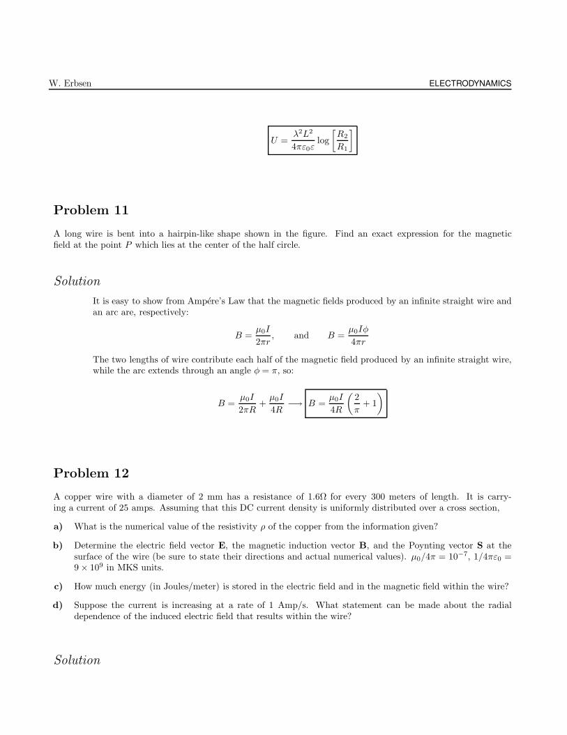
W. Erbsen ELECTRODYNAMICS
U =λ2L2
4πε0εlog
[R2
R1
]
Problem 11
A long wire is bent into a hairpin-like shape shown in the figure. Find an exact expression for the magneticfield at the point P which lies at the center of the half circle.
Solution
It is easy to show from Ampere’s Law that the magnetic fields produced by an infinite straight wire andan arc are, respectively:
B =µ0I
2πr, and B =
µ0Iφ
4πr
The two lengths of wire contribute each half of the magnetic field produced by an infinite straight wire,while the arc extends through an angle φ = π, so:
B =µ0I
2πR+µ0I
4R−→ B =
µ0I
4R
(2
π+ 1
)
Problem 12
A copper wire with a diameter of 2 mm has a resistance of 1.6Ω for every 300 meters of length. It is carry-ing a current of 25 amps. Assuming that this DC current density is uniformly distributed over a cross section,
a) What is the numerical value of the resistivity ρ of the copper from the information given?
b) Determine the electric field vector E, the magnetic induction vector B, and the Poynting vector S at thesurface of the wire (be sure to state their directions and actual numerical values). µ0/4π = 10−7, 1/4πε0 =9 × 10⁹ in MKS units.
c) How much energy (in Joules/meter) is stored in the electric field and in the magnetic field within the wire?
d) Suppose the current is increasing at a rate of 1 Amp/s. What statement can be made about the radialdependence of the induced electric field that results within the wire?
Solution
CHAPTER 5: DEPARTMENTAL EXAMINATIONS 423
a) The fundamental relation relating resistance and resistivity is:
R =ρL
A−→ ρ =
RA
L(5.2.43)
In our case, A = πr2 = π(10−3 m
)2, so that the resistivity is given by
ρ =(1.6Ω)(π(10−3m)2)
300m−→ ρ = 1.67× 10⁻⁸ Ω · m (5.2.44)
b) To find the electric field vector E, we must employ Gauss’ Law:∮
E · d` =1
ε0
λ
L−→ E · 2πr =
1
ε0
λ
L−→ E =
1
2πε0
λ
r(5.2.45)
We notice that the equaled part in (5.2.45) looks suspiciously similar to the definition of the scalarpotential V . And we can go ahead and find the scalar potential using the given information:V = IR = (25A)(1.6Ω) = 40v. Using this information, and manipulating (5.2.45), we have
E =
(1
4πε0
λL
r
)2
L=
2V
L(5.2.46)
Substituting the given values, (5.2.46) becomes:
E =2
15
v
mz (5.2.47)
The magnetic field may similarly be found using Ampere’s Law:∮
B · d` =µ0Ienc −→ B =µ0I
2πr=
2 × 10−7 · 25A
10−3m
Evaluating this, we arrive at
B = 5 × 10⁻³ T φ (5.2.48)
Using (5.2.47) and (5.2.48), we can calculate the Poynting Vector S:
S =1
µ0E × B =
1
µ0
(4
15
v
mz
)×
(3 × 10⁻³ T φ
)−→ S = −1061
W
m2ρ (5.2.49)
c) Finding the total energy stored in the both the electric and magnetic fields entails recalling thefollowing relations:
ηE =energy
volume=
1
2ε0|E|2, and ηB =
energy
volume=
1
2
1
µ0|B|2
Let’s say that we are interested in the amount of energy in a 1m length of wire. Then the volumeis V = πr2 = π(10−3 m)2(1 m) = 3.14× 10⁻⁶ m3. Accordingly, the amount of energy stored in theelectric and magnetic fields is given by
1
2
(8.887× 10⁻¹² A · s
V · m
) ∣∣∣∣2
15
v
m
∣∣∣∣2 (
3.14× 10⁻⁶ m3)−→ Energy in E = 2.473× 10⁻¹⁹ J
m
1
2
(1
4π10−7
A ·mV · s
)∣∣∣5 × 10⁻³ T φ
∣∣∣2 (
3.14× 10⁻⁶m3)−→ Energy in B = 1.562× 10⁻⁵ J
m
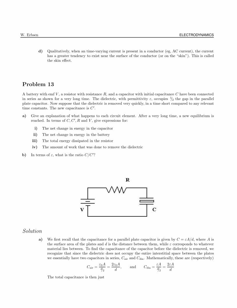
W. Erbsen ELECTRODYNAMICS
d) Qualitatively, when an time-varying current is present in a conductor (eg, AC current), the currenthas a greater tendency to exist near the surface of the conductor (or on the “skin”). This is calledthe skin effect.
Problem 13
A battery with emf V , a resistor with resistance R, and a capacitor with initial capacitance C have been connectedin series as shown for a very long time. The dielectric, with permittivity ε, occupies 1/2 the gap in the parallelplate capacitor. Now suppose that the dielectric is removed very quickly, in a time short compared to any relevanttime constants. The new capacitance is C ′.
a) Give an explanation of what happens to each circuit element. After a very long time, a new equilibrium isreached. In terms of C,C ′, R and V , give expressions for:
i) The net change in energy in the capacitor
ii) The net change in energy in the battery
iii) The total energy dissipated in the resistor
iv) The amount of work that was done to remove the dielectric
b) In terms of ε, what is the ratio C/C ′?
Solution
a) We first recall that the capacitance for a parallel plate capacitor is given by C = εA/d, where A isthe surface area of the plates and d is the distance between them, while ε corresponds to whatevermaterial lies between. To find the capacitance of the capacitor before the dielectric is removed, werecognize that since the dielectric does not occupy the entire interstitial space between the plateswe essentially have two capacitors in series, Cair and Cdia. Mathematically, these are (respectively)
Cair =ε0Ad/2
=2ε0A
d, and Cdia =
εAd/2
=2εA
d
The total capacitance is then just

CHAPTER 5: DEPARTMENTAL EXAMINATIONS 425
C =1
Cair+
1
Cdia=
CairCdia
Cair + Cdia=
(2ε0A/d)(2εA/d)
2ε0A/d+ 2εA/d=
2εε0A
d(ε+ ε0)(5.2.50)
While after the dielectric is removed, the capacitance is simply
C ′ =ε0A
d(5.2.51)
i) The amount of energy in the capacitor decreases. Adding dielectrics between the plates ofa capacitor act to decrease the magnitude of the electric field, but increase the capacitance(and therefore the energy stored) through the polarization of the static dielectric atoms. Tocalculate this change, we just have to remember that the amount of energy in a capacitor isjust U = 1/2CV
2. So,
∆Uc = 1/2C′V 2 − 1/2CV
2 −→ ∆Uc = 1/2V2 (C ′ −C) (5.2.52)
ii) When the dielectric is removed, there is a drop in capacitance and charge flows from the platesof the capacitor towards the battery. The change in energy of the circuit occurs due to thermallosses in the resistor; the potential energy of a charge in a potential is U = QV , so the changein energy is then
∆Ub = Q′V −QV = C ′V 2 − CV 2 −→ ∆Ub = (C ′ −C)V 2 (5.2.53)
iii) As mentioned previously, the total amount of energy dissipated in the circuit is done throughthe resistor. The basic equation to calculate this is P = I2R, however all we have to do is takethe difference of (5.2.52) and (5.2.53):
∆Ur = ∆Uc − ∆Ub = 1/2V2 (C ′ − C) − (C ′ −C)V 2 −→ ∆Ur = 1/2V
2 (−C ′ +C) (5.2.54)
The ratio of the capacitances before and after the dielectric is removed is
C
C ′ =2εε0A
d(ε+ ε0)· d
ε0A−→ C
C ′ =2ε
ε+ ε0
Problem 14
A series LCR circuit with L= 2 H, C=2 µF, and R=20 Ω is driven by a generator with maximum emf of 100 Vand variable frequency. Find the resonant frequency ω0 and the phase φ and maximum current Imax when thegenerator angular frequency is ω = 400 s−1.
Solution
We first recall that for a resonant RLC circuit, we have Z = R, ω = 1/√LC , XC = XL, and φ = 0. This
is not the case, however; the first thing we want to do is find the resonant frequency ω0 of the circuit:
ω0 =1√LC
=1√
(2 H)(2 × 10⁻⁶ F)−→ ω0 = 500
rad
sec(5.2.55)
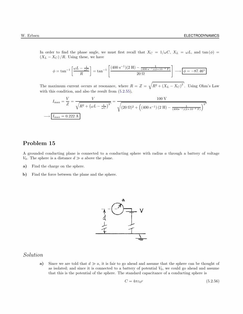
W. Erbsen ELECTRODYNAMICS
In order to find the phase angle, we must first recall that XC = 1/ωC, XL = ωL, and tan (φ) =(XL −XC ) /R. Using these, we have
φ = tan−1
[ωL − 1
ωC
R
]= tan−1
[(400 s−1)(2 H) − 1
(400 s−1)(2×10⁻⁶ F)
20 Ω
]−→ φ = −87.46o
The maximum current occurs at resonance, where R = Z =
√R2 + (XL −XC)
2. Using Ohm’s Law
with this condition, and also the result from (5.2.55),
Imax =V
Z=
V√R2 +
(ωL− 1
ωC
)2 =100 V√
(20 Ω)2 +((400 s−1) (2 H) − 1
(400s−1)(2×10⁻⁶ F)
)2
−→ Imax = 0.222 A
Problem 15
A grounded conducting plane is connected to a conducting sphere with radius a through a battery of voltageV0. The sphere is a distance d a above the plane.
a) Find the charge on the sphere.
b) Find the force between the plane and the sphere.
Solution
a) Since we are told that d a, it is fair to go ahead and assume that the sphere can be thought ofas isolated; and since it is connected to a battery of potential V0, we could go ahead and assumethat this is the potential of the sphere. The standard capacitance of a conducting sphere is
C = 4πε0r (5.2.56)
CHAPTER 5: DEPARTMENTAL EXAMINATIONS 427
Where in our case r = a. Furthermore, we know that Q = CV , so the total charge on our sphereis just
Q = 4πε0aV0 (5.2.57)
b) The force between the sphere and the grounded conducting plane can be calculated via the methodof images, where we imagine an identical, albeit oppositely charged sphere a distance 2d away. Using(5.2.57) and Coulomb’s law, we have
F =1
4πε0
Q2
(2d)2=
1
4πε0
(4πε0aV0)2
4d2
Which can be readily simplified to
F =πε0a
2V 20
d2
Problem 17
A conducting sphere of radius a and total charge Q is surrounded by a spherical shell of dielectric material(with permittivity ε) of inner radius a and outer radius b. Find the electrostatic energy of the system.
Solution
The general form for the energy stored in any electrostatic system is
W =ε
2
∫E2 dτ (5.2.58)
In our case, the electric field of the conducting sphere is given by
E =1
4πε
Q
r2r (5.2.59)
Inserting this value for E into (5.2.58), we have
W =ε
2
∫∫∫ (1
4πε
Q
r2r
)2
dV =ε
2
1
16π2ε2Q2
∫ 2π
0
∫ π
0
∫ ∞
0
1
r4· r2 sin θ drdθdϕ (5.2.60)
The radial integral in (5.2.60) must be divided according to each section: from 0 → a we are inside theconductor, so E = 0. However from a → b and b → ∞ we must evaluate the integral, and (5.2.60)becomes:
W =Q2
32π2ε20
∫ 2π
0
dϕ
∫ π
0
sin θ dθ
[ε20ε2
∫ b
a
1
r2dr +
∫ ∞
b
1
r2dr
]
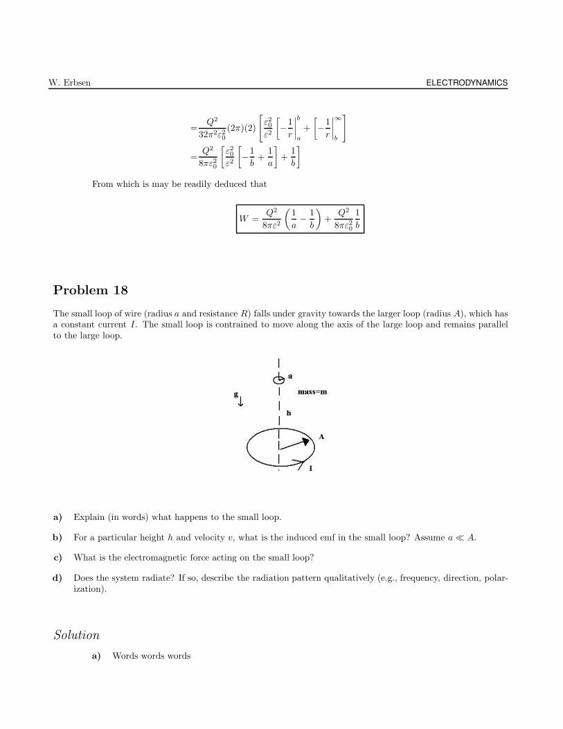
W. Erbsen ELECTRODYNAMICS
=Q2
32π2ε20(2π)(2)
[ε20ε2
[−1
r
∣∣∣∣b
a
+
[−1
r
∣∣∣∣∞
b
]
=Q2
8πε20
[ε20ε2
[−1
b+
1
a
]+
1
b
]
From which is may be readily deduced that
W =Q2
8πε2
(1
a− 1
b
)+
Q2
8πε20
1
b
Problem 18
The small loop of wire (radius a and resistance R) falls under gravity towards the larger loop (radius A), which hasa constant current I. The small loop is contrained to move along the axis of the large loop and remains parallelto the large loop.
a) Explain (in words) what happens to the small loop.
b) For a particular height h and velocity v, what is the induced emf in the small loop? Assume a A.
c) What is the electromagnetic force acting on the small loop?
d) Does the system radiate? If so, describe the radiation pattern qualitatively (e.g., frequency, direction, polar-ization).
Solution
a) Words words words
CHAPTER 5: DEPARTMENTAL EXAMINATIONS 429
b) The emf induced on the smaller loop will be due to the change of flux passing through it, changingas it falls:
E = −dΦB
dt= − d
dt
∮B · dA (5.2.61)
If we assume that the field is homogeneous throughout the smaller loop, we can expand on (5.2.61)as follows
E = − d
dtB · πa2 (5.2.62)
At this point all we have to do is find B. The best way to do this is with the Biot-Sevart Law, butbefore we do that we should define some needed quantities. d`, the length element of the sourceloop (the bigger one) is A dφ. Furthermore, the radial vector r is found by subtracting by boringtrig stuff: r = zk − Aρ. The magnitude of r is just
√z2 +A2 . Using all this in the Biot-Sevart
Law:
B =µ0I
4π
d` × r
|r|3
=µ0I
4π
A dφφ × (zk −Aρ)
(z2 + A2)3/2
=µ0IA
4π
zρ + Az
(z2 +A2)3/2
dφ
=µ0IA
4π
1
(z2 +A2)3/2
[z
∫ 2π
0
ρ dφ+ A
∫ 2π
0
z dφ
]
=µ0I
4π
A
(z2 +A2)3/2
[0 + 2πA] z]
=µ0I
2
A2
(z2 +A2)3/2
z (5.2.63)
We can now use (5.2.63) in (5.2.62) to find E:
E = − πa2 d
dt
[µ0I
2
A2
(z2 +A2)3/2
]
= − πµ0Ia2A2
2
d
dt
dt
dz
dz
dt
[1
(z2 +A2)3/2
]
= − πµ0Ia2A2
2z
d
dz
[1
(z2 +A2)3/2
]
= − πµ0Ia2A2
2z
d
dz
[− 3z
(z2 + A2)5/2
∣∣∣∣∣z=h
(5.2.64)
By evaluating (5.2.64) at z = h, and recognizing that z is the downward velocity, we have
E =3hµ0Iπa
2A2
2(h2 +A2)5/2
· v (5.2.65)
W. Erbsen ELECTRODYNAMICS
c) Not too sure on this one
d) Yes , the system does radiate, in the ρ direction.
Problem 19
A cylindrically shaped conductor has length L, radius a, and conductivity σ. It carries a uniform time-independentcurrent density J = J e0, parallel to its long axis.
a) Determine the electric and magnetic fields within the conductor.
b) Calculate the Poynting vector S within the conductor.
c) Write out Poynting’s theorem for this situation. Verify that it is satisfied for any point within the conductor.
Solution
a) We first recall the fundamental relation for current density: J = σE. So, the electric field is givensimply by
E =
J/σ z for 0 ≤ ρ ≤ a0 elsewhere
(5.2.66)
And to find the internal magnetic field B, we apply Ampere’s Law:∮
B · d` =µ0Iinc = µ0
(πρ2J
)
2πρB =µπρ2J
Such that we have
B =
µ0Jρ/2 φ for 0 ≤ ρ ≤ a0 elsewhere
(5.2.67)
b) We note that the Poynting vector takes the form
S =1
µ0E × B
And since we know that E = J/σ ρ from (5.2.66) and B = µ0Jρ/2 ρ from (5.2.67), then thePoynting vector is simply
S =J2ρ
2σ(−ρ) (5.2.68)
CHAPTER 5: DEPARTMENTAL EXAMINATIONS 431
c) Poynting’s theorem states that
∂u
∂t+ ∇ · S = − J · E (5.2.69)
Where u is the energy density. We can express the energy density as:
u =1
2
(ε0E
2 +B2
µ0
)(5.2.70)
Substituting (5.2.66) and (5.2.67) into (5.2.70),
u =1
2
(ε0
J2
σ2+ µ0
µ20J
2ρ2
4
)
=1
2
(ε0
J2
σ2+µ0J
2ρ2
4
)(5.2.71)
And we note that u is time independent, so ∂u/∂t = 0. We also note that the divergence incylindrical coordinates takes the form
∇ · F =1
ρ
∂
∂ρ(ρFρ) +
1
ρ
∂Fϕ
∂ϕ+∂Fz
∂z
So finally we can calculate
∇ · S =1
ρ
∂
∂ρ(ρSρ) +
1
ρ
∂Sϕ
∂ϕ+∂Sz
∂z
=1
ρ
∂
∂ρ(ρSρ)
=1
ρ
∂
∂ρ
(ρJ2ρ
2σ(−ρ)
)
=1
ρ
J2ρ
σ(−ρ)
= − J2
σρ (5.2.72)
So, using (5.2.72), Poynting’s theorem (5.2.69) is now
−J2
σρ = −J · E = −J
J
σρ = −J2
σρ X
Problem 21
An electron beam of uniform charge density ρ0 inside the beam radius r0 is traveling on the axis of a metaltube with an inner radius Ri and an outer radius of Ro which is kept at a potential φτ .
a) Calculate the potential at the center of the electron beam.
b) Calculate the net charge on the tube per unit length `.
W. Erbsen ELECTRODYNAMICS
c) Calculate the energy that is required to double the tube potential to 2×φτ assuming that the electron beamcharge density remains constant.
Solution
a) Calculating the potential at the center of the beam poses no major obstacles. We imagine to bedragging a unit charge (“test” charge) from ∞ to the center of the beam . The total potential ishow much work it took. So we start from the outside, from ∞, and boundary by boundary calculatethe potentials and at the end add them together.
φ(r = 0) = −∫ 0
∞E · ds
= −∫ Ro
∞E4 · ds
︸ ︷︷ ︸φτ
−∫ Ri
Ro
E3 · ds−∫ Ra
Ri
E2 · ds−∫ 0
a
E1 · ds (5.2.73)
We are told that the potential of the shell is kept at φτ , so we needn’t even calculate E4. The restare
E1 =ρ0(πr
2)
2πε0r =
ρ0
2ε0r r (5.2.74a)
E2 =ρ0(πr
20)
2πε0rr =
ρ0r20
2ε0rr (5.2.74b)
E3 =0 (5.2.74c)
The reason why E3 = 0 is because this region corresponds to within a conductor, where the internalelectric field is guaranteed to be zero. Using (5.2.74a), (5.2.74b) and (5.2.74c), we can evaluate ourpotential from (5.2.73):
φ(0) =φτ −∫ Ra
Ri
ρ0r20
2ε0rr · dr −
∫ 0
a
ρ0
2ε0r r · dr
=φτ − ρ0r20
2ε0
∫ Ro
Ri
1
rdr − ρ0
2ε0
∫ 0
a
r dr
=φτ − ρ0r20
2ε0[log r|Ro
Ri− ρ0
2ε0
[r2
2
∣∣∣∣0
a
=φτ − ρ0r20
2ε0log
[Ri
Ro
]+
ρ0
2ε0
a2
2(5.2.75)
From (5.2.75) it is easy to see that the potential is
φ(0) = φτ +ρ0r
20
2ε0log
[Ri
Ro
]+ρ0a
2
4ε0
b) The net charge on the tube per unit length would just be the charge density times the area inquestion where we take the length to be equal to 1,
λ = −ρ0πa2
CHAPTER 5: DEPARTMENTAL EXAMINATIONS 433
Problem 22
A charge 2q is located at (0, 0, 0), a second charge, −q, is located at (0,−a, 0), and a third charge, −q, is lo-cated at (0, 0,−a).
a) Calculate the monopole and dipole moments.
b) Calculate all quadrupole moments.
c) What is the potential for r a using multipole approximation?
Solution
a) The monopole moment is zero, since it is just the sum of the charges. The dipole moment for anarray of charges is defined by
p =
N∑
i=1
riqi (5.2.76)
Applied to our geometric arrangement of charges,
p = (−aj)(−q) + (0)(2q) + (−ak)(−q) −→ p = aq(j + k) (5.2.77)
b) The defining equation for the quadrupole moment is
Q0 =1
2
∞∑
i=1
qi
(3xiαxiβ − r2i δαβ
)(5.2.78)
Applying (5.2.78) to our case,
Q0 = −1
2(a2)(−q) +
1
2(0)(−2q) − 1
2(a2)(−q) −→ Q0 = a2q (5.2.79)
c) The full equation for multipole expansion is
V (r) =1
4πε0
∞∑
n=0
1
r(n+1)
∫(r′)nPn(cos θ′)ρ(r′) dτ ′
=1
4πε0
[1
r
∫ρ(r′) dτ ′ +
1
r2
∫r′ cos θ′ρ(r′) dτ ′ +
1
r3
∫(r′)2
(3
2cos2 θ′ − 1
2
)ρ(r′) dτ ′ + ...
]
(5.2.80)
The integrals represent the various -pole terms through quadrupole. We know that the monopoleterm is zero, so we simply substitute (5.2.77) and (5.2.79) into (5.2.80):
V (r) ≈ 1
4πε0
[aq(j + k)
r2+a2q
r2
]
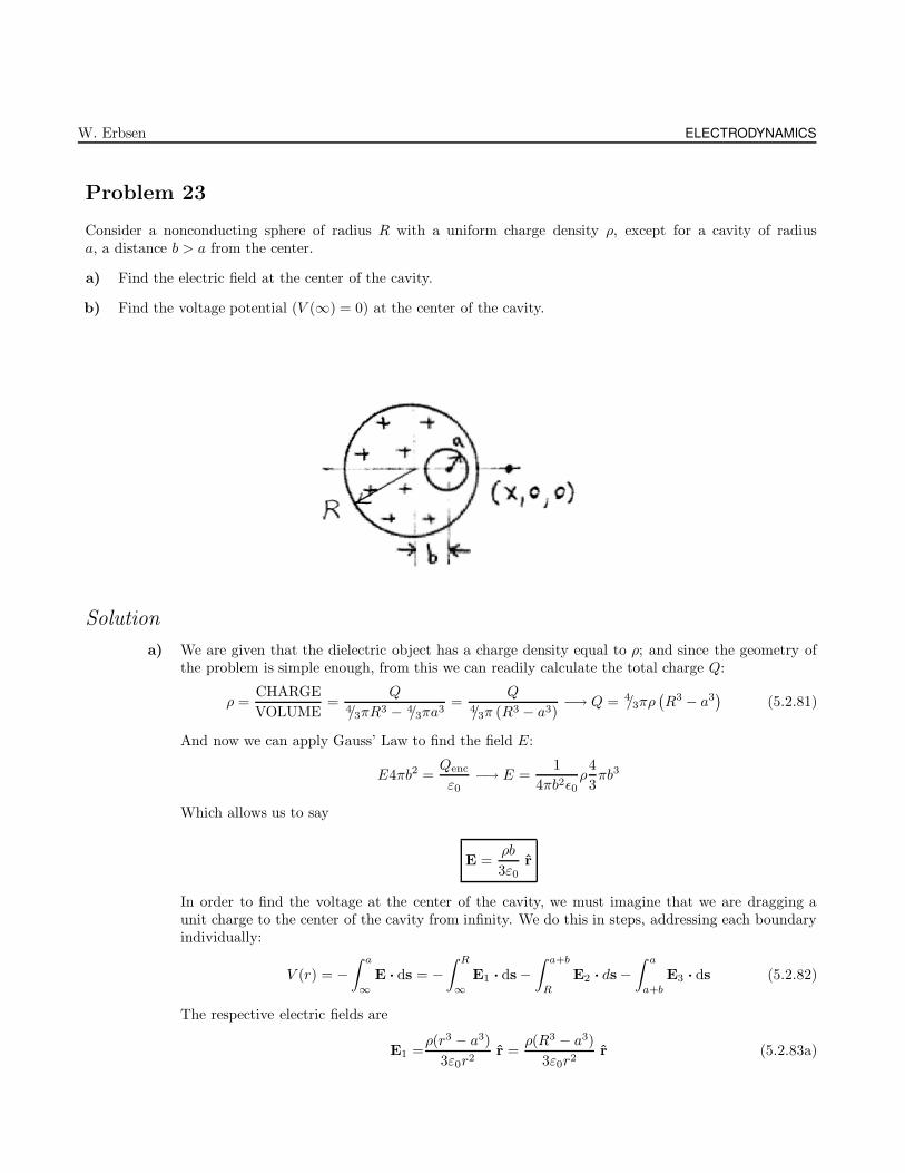
W. Erbsen ELECTRODYNAMICS
Problem 23
Consider a nonconducting sphere of radius R with a uniform charge density ρ, except for a cavity of radiusa, a distance b > a from the center.
a) Find the electric field at the center of the cavity.
b) Find the voltage potential (V (∞) = 0) at the center of the cavity.
Solution
a) We are given that the dielectric object has a charge density equal to ρ; and since the geometry ofthe problem is simple enough, from this we can readily calculate the total charge Q:
ρ =CHARGE
VOLUME=
Q4/3πR3 − 4/3πa3
=Q
4/3π (R3 − a3)−→ Q = 4/3πρ
(R3 − a3
)(5.2.81)
And now we can apply Gauss’ Law to find the field E:
E4πb2 =Qenc
ε0−→ E =
1
4πb2ε0ρ4
3πb3
Which allows us to say
E =ρb
3ε0r
In order to find the voltage at the center of the cavity, we must imagine that we are dragging aunit charge to the center of the cavity from infinity. We do this in steps, addressing each boundaryindividually:
V (r) = −∫ a
∞E · ds = −
∫ R
∞E1 · ds−
∫ a+b
R
E2 · ds−∫ a
a+b
E3 · ds (5.2.82)
The respective electric fields are
E1 =ρ(r3 − a3)
3ε0r2r =
ρ(R3 − a3)
3ε0r2r (5.2.83a)
CHAPTER 5: DEPARTMENTAL EXAMINATIONS 435
E2 =ρ(r3 − a3)
3ε0r2r (5.2.83b)
E3 =ρb
3ε0r (5.2.83c)
We now substitute (5.2.83a)-(5.2.83c) into (5.2.82) and integrate. I will do each of the three integralsin turn and combine them later. The first is
V1(r) =ρ(R3 − a3)
3ε0
∫ R
∞
1
r2dr
= −[ρ(R3 − a3)
3ε0r
∣∣∣∣R
∞
= − ρ(R3 − a3)
3ε0R(5.2.84)
And now for the second,
V2(r) =ρ
3ε0
∫ a+b
R
r3 − a3
r2dr
=ρ
3ε0
[∫ a+b
R
rdr − a3
∫ a+b
R
1
r2dr
]
=ρ
3ε0
[[r2
2
∣∣∣∣a+b
R
− a3
[−1
r
∣∣∣∣a+b
R
]
=ρ
3ε0
[(a + b)2
2− R2
2+
1
a+ b− 1
R
](5.2.85)
And that last little bitch is
V3(r) =ρb
3ε0
∫ a
a+b
dr
=ρb
3ε0[a− (a + b)]
= − ρb2
3ε0(5.2.86)
We now take (5.2.84) - (5.2.86) and substitute it into (5.2.82):
V (r) =ρ(R3 − a3)
3ε0R+
ρ
3ε0
[(a+ b)2
2− R2
2+
1
a+ b− 1
R
]+ρb2
3ε0
Which finally leads us to
V (r = 0) =ρ
3ε0
[(R3 − a3)
R+
(a + b)2
2− R2
2+
1
a + b− 1
R+ b2
]
Problem 24
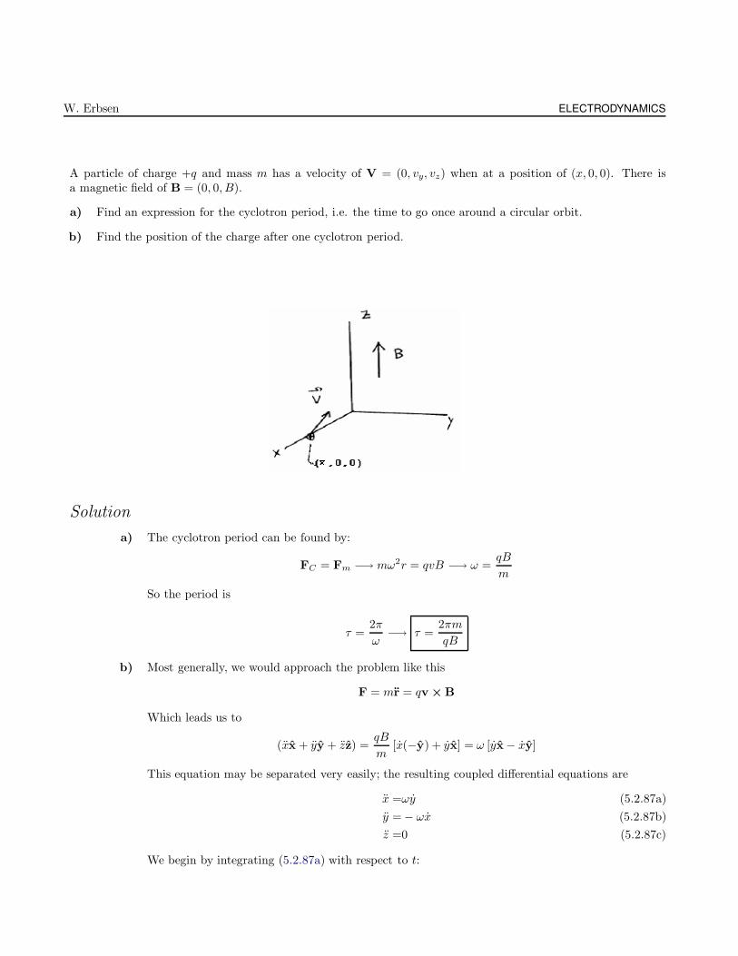
W. Erbsen ELECTRODYNAMICS
A particle of charge +q and mass m has a velocity of V = (0, vy, vz) when at a position of (x, 0, 0). There isa magnetic field of B = (0, 0, B).
a) Find an expression for the cyclotron period, i.e. the time to go once around a circular orbit.
b) Find the position of the charge after one cyclotron period.
Solution
a) The cyclotron period can be found by:
FC = Fm −→ mω2r = qvB −→ ω =qB
m
So the period is
τ =2π
ω−→ τ =
2πm
qB
b) Most generally, we would approach the problem like this
F = mr = qv × B
Which leads us to
(xx + yy + zz) =qB
m[x(−y) + yx] = ω [yx− xy]
This equation may be separated very easily; the resulting coupled differential equations are
x =ωy (5.2.87a)
y = − ωx (5.2.87b)
z =0 (5.2.87c)
We begin by integrating (5.2.87a) with respect to t:
CHAPTER 5: DEPARTMENTAL EXAMINATIONS 437
x = ωy + C(vx) (5.2.88)
Substituting (5.2.88) into (5.2.87b),
y = −ω2y − ωC(vx) (5.2.89)
Our initial conditions state that at t = 0 then vx = 0, so C(vx) in (5.2.89) vanishes. We are leftwith a second order differential equation, with solutions of the form
y(t) = A cosωt+ B sinωt
If we again apply our initial conditions, we note that at t = 0 then y = 0, so we must require thatA = 0. Our solution is then
y(t) = B sinωt (5.2.90)
We now substitute (5.2.90) into (5.2.88):
x = ωyB sinωt −→ x(t) = −B cosωt +C(x) −→ x(t) = −B cosωt + x0 (5.2.91)
Where we note that initial conditions imply that C(x) is none other than the initial position of ourparticle. Additionally, we can unleash the true identity of the integration constant B everpresentin both (5.2.90) and (5.2.91). We do this by taking the derivative of (5.2.90) and setting it equalto vy:
y(t) = Bω cos 0 = vy −→ B =vy
ω
And now we can rewrite (5.2.90) and (5.2.91):
x(t) = − vy
ωcosωt + x0 (5.2.92a)
y(t) =vy
ωsinωt (5.2.92b)
And now, after one full period, t → τ , which implies that ωτ = 2π, it can be easily (very easily)seen that (5.2.92a) and (5.2.92b) reveal the location of the particle to be
x(τ ) = x0 −vy
ω, y(τ ) = 0
Problem 25
A long wire lies along the z-axis. A square coil of wire, each side of length a, lies in the xz-plane. The sidenearest the wire is parallel to the wire and located at x = a.
a) Find the vector potential A if the wire is carrying a current I and there is no current in the loop.
b) What is the flux through the loop, using the results from part a)?
c) What is the mutual inductance of the loop and on the wire?
W. Erbsen ELECTRODYNAMICS
d) If the current I is varying at a rate dI/dt = K, what is the induced emf in the coil?
e) If there is a current in the loop varying at a rate dI/dt = C, what is the size of the voltage across the endsof the long wire?
Solution
a) In order to find the magnetic vector potential A, we must “uncurl” it from B = ∇ × A. We dothis by first setting up the determinant,
∣∣∣∣∣∣∣∣∣
ρ φ z
∂
∂ρ
1
ρ
∂
∂φ
∂
∂z
Aρ Aφ Az
∣∣∣∣∣∣∣∣∣
Due to the geometry of this particular problem, since I flows along the z direction and the face ofthe loop is adjacent aligned to the wire, we can make some shortcuts. We know that A only flowsin the z direction in our case, so the other terms are zero. Additionally, we can see that A willdepend only on ρ, so any derivatives of A that aren’t with respect to ρ will be zero.
∣∣∣∣∣∣∣∣∣
ρ φ z
∂
∂ρ0 0
0 0 Az
∣∣∣∣∣∣∣∣∣= − ∂
∂ρAz φ
So, we now have
B = ∇ × A = − ∂
∂ρAzφ =
µ0I
2πρ(5.2.93)
The differential equation in (5.2.93) can be solved straightforwardly,
∂
∂ρAzφ =
µ0I
2πρφ −→ Az =
µ0I
2πlog
[a
ρ
](5.2.94)
b) To find the flux, we use the typical definitions:
ΦB =
∫B · dA =
∫(∇ × A) · dA =
∫µ0I
2πρdρdz =
µ0I
2π
∫ 2a
a
1
ρdρ
∫ a
0
dz (5.2.95)
The integration in (5.2.95) is straightforward, and the result is
ΦB =µ0Ia
2πlog [2] (5.2.96)
c) If we recall that the mutual inductance is qualitatively defined as M = ΦB/I, then the mutualinductance is simply:
M =µ0a
2πlog [2]
CHAPTER 5: DEPARTMENTAL EXAMINATIONS 439
d) Using (5.2.96), we can straightforwardly find the emf to be
E = −dΦB
dt= − d
dt
µ0Ia
2πlog [2] = −µ0a
2πlog [2]
dI
dt
And using the handy substitution the prompt suggests,
E = −Kµ0a
2πlog [2]
e) With the given substitution, the voltage across the ends of the long wire is
E = −Cµ0a
2πlog [2]
Problem 26
A disc carrying a uniform surface charge density σ has radius a and rotates at an angular frequency ω. Thisdisc lies in the xy-plane and rotates along the z-axis. A second identical disc rotating at the same frequency islocated with its center on the z-axis at Z, but this one lies in the yz-plane about an axis parallel to the x-axis.Find the torque on the second disc. Indicate in a sketch the direction of the torque and the sense of rotation ofthe two discs.
Solution
We begin by recanting a rather unfamiliar form of Biot-Sevart’s Law:
dB =µ0
4π
KdS × r
|r|3 (5.2.97)
Where K is known as the surface charge density, and is described by K = σv. Similar to what we did ina previous problem, we define all the elements needed to compute the magnetic field from (5.2.97). Theline element and its magnitude are, respectively
r = zz − ρρ, and |r| =√z2 + ρ2
And we can also expand upon the surface charge density:
K = σv = σωρφ
And we also recall that that the volume element for cylindrical coordinates is ds = ρ dρdφ. We can nowcalculate,
Kds × r =(σωρρ) (ρ dρdφ) × (zz − ρρ)
=σωρ2 dρdφφ × (zz − ρρ)
W. Erbsen ELECTRODYNAMICS
=σωρ2 dρdφ (zρ + ρz) (5.2.98)
We can now substitute (5.2.98) into (5.2.97),
dB =µ0σω
4π
ρ2 (zρ + ρz)
(z2 + ρ2)3/2
dρdφ
B =µ0σω
4π
∫∫ρ2 (zρ + ρz)
(z2 + ρ2)3/2
dρdφ
=µ0σω
2
[z
∫ a
0
ρ2
(z2 + ρ2)3/2
ρ dρ+
∫ a
0
ρ3
(z2 + ρ2)3/2
z dρ
](5.2.99)
The first integral in (5.2.99) is neglected, due to symmetry. The second integral can be found in tables,and the result is
B =µ0σω
2
[a2 + 2z2
√z2 + a2
− 2z
]z (5.2.100)
Now, if we can reconcile with the fact that K = σv, then we can find the magnetic moment of the upperloop as follows
µ =
∫ a
0
I · dρ =
∫ a
0
K(πρ2) dρ =
∫ a
0
σv(πρ2) dρ =
∫ a
0
σωρ(πρ2) dρ = πσω
∫ a
0
ρ3 dρ =πσωa4
4(5.2.101)
And if we recall that within this context τ = µ × B, then by using (5.2.100) and (5.2.101) we can findthe torque:
τ =πµ0σ
2ω2a4
8
[a2 + 2z2
√z2 + a2
− 2z
](−y)
Problem 27
The KSU ultra-short pulse, ultra-high intensity laser in the JRM Lab has λ = 800 nm, pulse width of 20 femtosec-onds, pulse energy of 6 mJ, and can be focused to a spot size of 100 µm.
a) What is the intensity of the light in the focus?
b) What average electric field produces this intensity?
c) To how many atomic units of the intensity and electric field does this correspond?
Solution
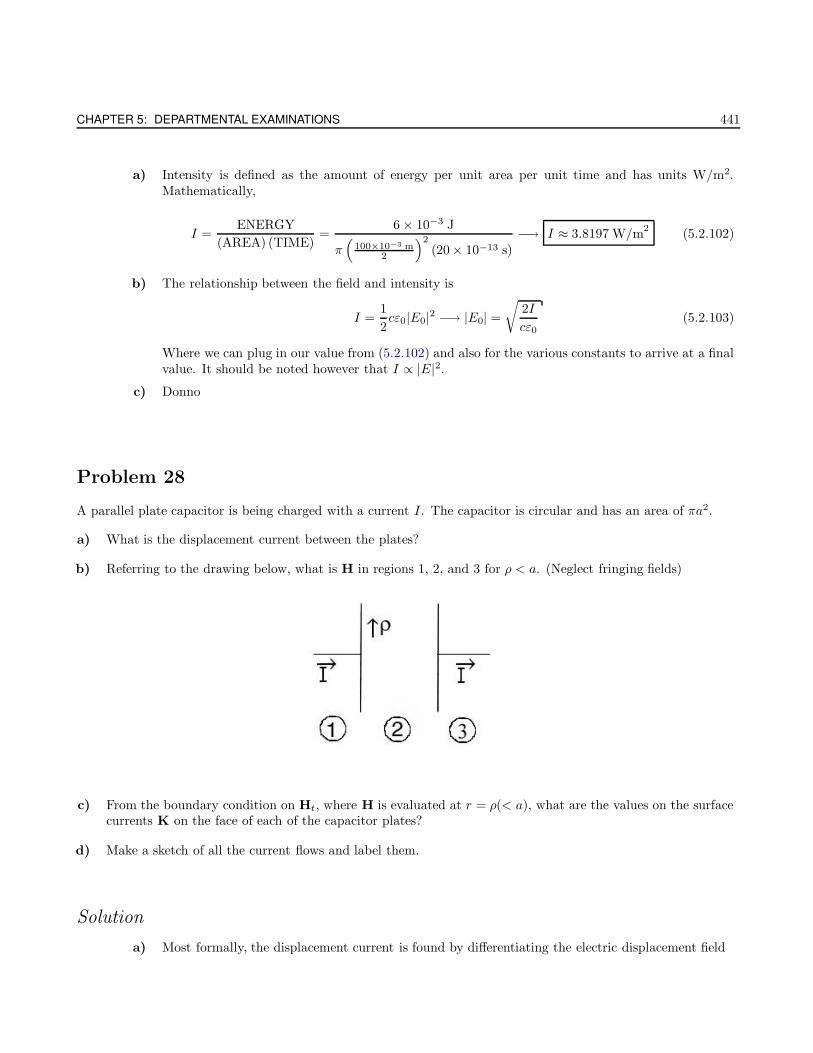
CHAPTER 5: DEPARTMENTAL EXAMINATIONS 441
a) Intensity is defined as the amount of energy per unit area per unit time and has units W/m2.Mathematically,
I =ENERGY
(AREA) (TIME)=
6 × 10⁻³ J
π(
100×10−3 m2
)2
(20× 10−13 s)−→ I ≈ 3.8197 W/m
2(5.2.102)
b) The relationship between the field and intensity is
I =1
2cε0|E0|2 −→ |E0| =
√2I
cε0(5.2.103)
Where we can plug in our value from (5.2.102) and also for the various constants to arrive at a finalvalue. It should be noted however that I ∝ |E|2.
c) Donno
Problem 28
A parallel plate capacitor is being charged with a current I. The capacitor is circular and has an area of πa2.
a) What is the displacement current between the plates?
b) Referring to the drawing below, what is H in regions 1, 2, and 3 for ρ < a. (Neglect fringing fields)
c) From the boundary condition on Ht, where H is evaluated at r = ρ(< a), what are the values on the surfacecurrents K on the face of each of the capacitor plates?
d) Make a sketch of all the current flows and label them.
Solution
a) Most formally, the displacement current is found by differentiating the electric displacement field
W. Erbsen ELECTRODYNAMICS
D = ε0E + P
↓ ↓ ↓
Jd = ε0∂E
∂t+
∂P
∂t
We have no dielectric so the polarization term is neglected in our case. One thing that shoulddefinitely be remembered is that the electric field between the plates of a parallel plate capacitoris E = σ/ε0. We are now in a place to find the displacement current Jd:
Jd = ε0∂E
∂t= ε0
∂
∂t
(σ
ε0
)=∂σ
∂t=
∂
∂t
(Q(t)
πa2
)(5.2.104)
If we recall that I(t) = Q(t), then (5.2.104) is
Jd =I
πa2z (5.2.105)
b) Recall that Ampere’s Law for H fields is∮
H · d` = Id
Within region 2, we can use (5.2.105) to find H:
H2(2πρ) =I
πa2φ −→ H2 =
I
2πρφ (5.2.106)
And in regions 1 and 3, the value for H is simply
H1,3 =I
2πρφ (5.2.107)
Problem 29
A spherical conductor A contains two spherical cavities. The total charge on A itself is zero. However, thereis a point charge qb at the center of one cavity, and qc at the center of the other. A considerable distance r awayis another charge qd. What force acts on each of the four objects A, qb, qc, and qd? Which answers, if any, are onlyapproximate? If qb is displaced slightly away from the center of the cavity, will it experience a resistance force?(If so, what is it?)
Solution
The forces on charges qb and qc themselves are, of course, zero. To calculate the force of qd acting on A,
F =1
4πε0
qd(qb + qc)
r2(5.2.108)
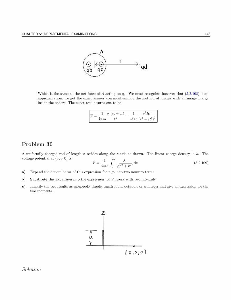
CHAPTER 5: DEPARTMENTAL EXAMINATIONS 443
Which is the same as the net force of A acting on qd. We must recognize, however that (5.2.108) is anapproximation. To get the exact answer you must employ the method of images with an image chargeinside the sphere. The exact result turns out to be
F =1
4πε0
qd(qb + qc)
r2− 1
4πε0
q2Rr
(r2 −R2)2
Problem 30
A uniformily charged rod of length a resides along the z-axis as drawn. The linear charge density is λ. Thevoltage potential at (x, 0, 0) is
V =1
4πε0
∫ a
0
λ√z2 + x2
dz (5.2.109)
a) Expand the denominator of this expression for x z to two nonzero terms.
b) Substitute this expansion into the expression for V , work with two integrals.
c) Identify the two results as monopole, dipole, quadrupole, octapole or whatever and give an expression for thetwo moments.
Solution
W. Erbsen ELECTRODYNAMICS
a) The series expansion around z is
1√z2 + x2
=1
x√z2/x2 + 1
=1
x− z2
2x3+
3z4
8x5− 5z6
16x7− ...
So, expanded to the first two nonzero terms:
1√z2 + x2
=1
x− z2
2x3(5.2.110)
b) Substituting (5.2.110) into (5.2.109), we have
V =1
4πε0
∫ a
0
λ
(1
x− z2
2x3
)dz
=1
4πε0λ
[1
x
∫ a
0
dz − 1
2x3
∫ a
0
z2 dz
]
=1
4πε0λ
[a
x− a3
6x3
]
So the result is
V =λ
4πε0
a
x− λ
24πε0
a3
x3(5.2.111)
c) The first term in (5.2.111) is monopole, because of the 1/x factor, and the second is quadrupole,since it has a 1/x3 term.
Problem 31
a) Find the voltage potential at point P a distance b from the right end of a uniform line charge with length `and total charge Q as drawn.
b) Using this voltage find the x-component of the electric field at point P .
Solution
a) We first note that our object has a charge given by dq = λ d`, and the total charge is Q, and thetotal length is `, so we know that λ = Q/`. Furthermore, we know that E = −∇V −→ dV = −Edx.We can take this further:
V = − λ
4πε0
∫ 0
−`
1
(b− x)dx
= − 1
4πε0
Q
`[log (b− x)|0−`
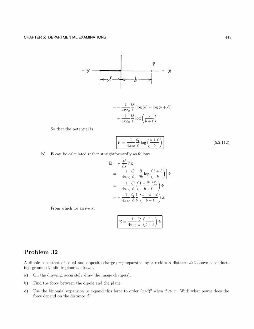
CHAPTER 5: DEPARTMENTAL EXAMINATIONS 445
= − 1
4πε0
Q
`[log (b) − log (b+ `)]
= − 1
4πε0
Q
`log
(b
b+ `
)
So that the potential is
V =1
4πε0
Q
`log
(b+ `
b
)(5.2.112)
b) E can be calculated rather straightforwardly as follows
E = − ∂
∂xV x
= − 1
4πε0
Q
`
[∂
∂blog
(b+ `
b
)]x
= − 1
4πε0
Q
`
(1 − (b+`)/bb+ `
)x
= − 1
4πε0
Q
`
1
b
(b− b− `
b+ `
)x
From which we arrive at
E =1
4πε0
Q
b
(1
b+ `
)x
Problem 32
A dipole consistent of equal and opposite charges ±q separated by x resides a distance d/2 above a conduct-ing, grounded, infinite plane as drawn.
a) On the drawing, accurately draw the image charge(s).
b) Find the force between the dipole and the plane.
c) Use the binomial expansion to expand this force to order (x/d)2 when d x. With what power does theforce depend on the distance d?
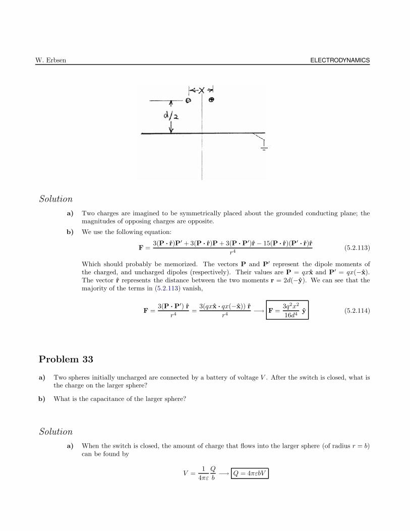
W. Erbsen ELECTRODYNAMICS
Solution
a) Two charges are imagined to be symmetrically placed about the grounded conducting plane; themagnitudes of opposing charges are opposite.
b) We use the following equation:
F =3(P · r)P′ + 3(P · r)P + 3(P · P′)r − 15(P · r)(P′
· r)r
r4(5.2.113)
Which should probably be memorized. The vectors P and P′ represent the dipole moments ofthe charged, and uncharged dipoles (respectively). Their values are P = qxx and P′ = qx(−x).The vector r represents the distance between the two moments r = 2d(−y). We can see that themajority of the terms in (5.2.113) vanish,
F =3(P · P′) r
r4=
3(qxx · qx(−x)) r
r4−→ F =
3q2x2
16d4y (5.2.114)
Problem 33
a) Two spheres initially uncharged are connected by a battery of voltage V . After the switch is closed, what isthe charge on the larger sphere?
b) What is the capacitance of the larger sphere?
Solution
a) When the switch is closed, the amount of charge that flows into the larger sphere (of radius r = b)can be found by
V =1
4πε
Q
b−→ Q = 4πεbV
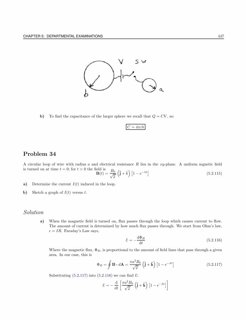
CHAPTER 5: DEPARTMENTAL EXAMINATIONS 447
b) To find the capacitance of the larger sphere we recall that Q = CV , so:
C = 4πεb
Problem 34
A circular loop of wire with radius a and electrical resistance R lies in the xy-plane. A uniform mgnetic fieldis turned on at time t = 0; for t > 0 the field is
B(t) =B0√2
(j + k
)[1 − e−λt
](5.2.115)
a) Determine the current I(t) induced in the loop.
b) Sketch a graph of I(t) versus t.
Solution
a) When the magnetic field is turned on, flux passes through the loop which causes current to flow.The amount of current is determined by how much flux passes through. We start from Ohm’s law,ε = IR. Faraday’s Law says,
E = −dΦB
dt(5.2.116)
Where the magnetic flux, ΦB, is proportional to the amount of field lines that pass through a givenarea. In our case, this is
ΦB =
∮B · dA =
πa2B0√2
(j + k
)[1 − e−λt
](5.2.117)
Substituting (5.2.117) into (5.2.116) we can find E:
E = − d
dt
[πa2B0√
2
(j + k
) [1 − e−λt
]]
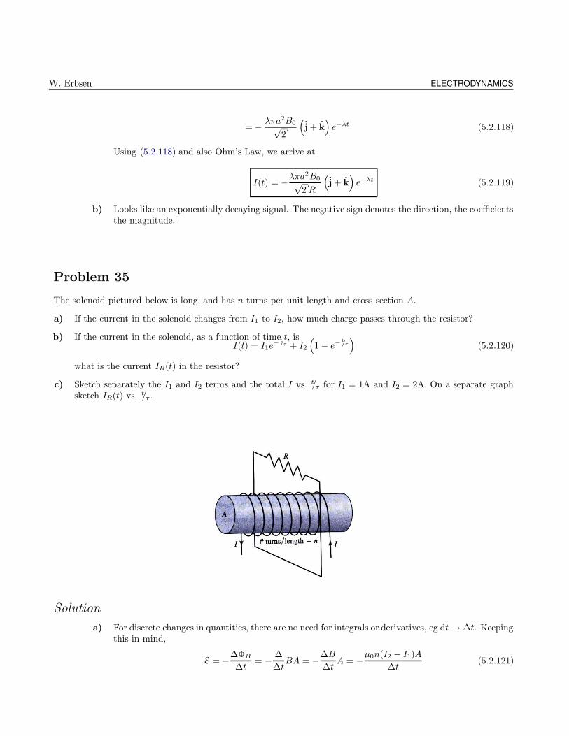
W. Erbsen ELECTRODYNAMICS
= − λπa2B0√2
(j + k
)e−λt (5.2.118)
Using (5.2.118) and also Ohm’s Law, we arrive at
I(t) = −λπa2B0√
2R
(j + k
)e−λt (5.2.119)
b) Looks like an exponentially decaying signal. The negative sign denotes the direction, the coefficientsthe magnitude.
Problem 35
The solenoid pictured below is long, and has n turns per unit length and cross section A.
a) If the current in the solenoid changes from I1 to I2, how much charge passes through the resistor?
b) If the current in the solenoid, as a function of time t, isI(t) = I1e
− t/τ + I2
(1 − e−
t/τ
)(5.2.120)
what is the current IR(t) in the resistor?
c) Sketch separately the I1 and I2 terms and the total I vs. t/τ for I1 = 1A and I2 = 2A. On a separate graphsketch IR(t) vs. t/τ .
Solution
a) For discrete changes in quantities, there are no need for integrals or derivatives, eg dt→ ∆t. Keepingthis in mind,
E = −∆ΦB
∆t= − ∆
∆tBA = −∆B
∆tA = −µ0n(I2 − I1)A
∆t(5.2.121)
CHAPTER 5: DEPARTMENTAL EXAMINATIONS 449
We also know Ohm’s Law, which states that E = IR, where I = ∆Q/(∆t). With this knowledge,(5.2.121) becomes
∆Q
∆tR = −µ0n(I2 − I1)A
∆t
From which it is clear that the ∆t on the denominator cancels, and we are left with
∆Q = −µ0n(I2 − I1)A
R
b) To calculate the current,
E = − ∂
∂tBA = − ∂
∂tµ0nIA = −µ0nA
∂I(t)
∂t(5.2.122)
Recalling again Ohm’s Law, IR(t) can be found by combining (5.2.122) and (5.2.120):
IR(t) =E
R= −µ0nA
R
∂
∂t
[I1e
− t/τ + I2
(1 − e−
t/τ
)]= −µ0nA
R
[−I1τe−
t/τ +I2τe−
t/τ
]
From which it is easily seen that
IR(t) = −µ0nA
Rτe−
t/τ [I2 − I1]
5.3 Modern Physics
Problem 1
Recently, 2000 rubidium atoms (8737Rb), which had been compressed to a density of 1013 atoms/cm3, were ob-
served to undergo a Bose-Einstein condensation as a function of temperature. This occurs when the deBrogliewavelengths overlap and the system forms a single macroscopic quantum state. Estimate the temperature at whichBose-Einstein condensation occurs for this system.
Solution
We first recall that the deBroglie wavelength is given by
λ =h
p(5.3.1)
Where we are also told that
N =2000 atoms
ρ =1013 atoms · cm3
W. Erbsen MODERN PHYSICS
So, we can say that the spacing is proportional to the deBroglie wavelength, and the spacing can befound by
2000 atoms
L3= 1013 atoms · cm3 −→ L =
(2000 atoms
1013 atoms · cm3
)1/3
(5.3.2)
We now wish to set (5.3.2) equal to the deBroglie wavelength. But first, we recall that
p =√
2mEE ∼ kBT
→ p ∼
√2mkBT (5.3.3)
Where putting (5.3.3) into (5.3.1) of course yields
λ ∼ h√2mkBT
(5.3.4)
Setting (5.3.4) equal to (5.3.2) yields
(2000 atoms
1013 atoms · cm3
) 1/3
=h√
2mkBT
Solving for T leaves us with
T ∼ h1/2
2mkB
(2000 atoms
1013 atoms · cm3
) 1/6
Problem 2
Rutile, TiO2, is a tetragonal crystal a = 4.4923A. The position of the Ti atoms in the unit cell are 0, 0, 0;1/2,
1/2,1/2 and the position of the oxygen atoms are 0.31, 0.31, 0; 0.81, 0.19, 0.5; 0.69, 0.69, 0; 0.19, 0.81, 0.5.
a) What would be the d-spacing of the 310 planes of rutile?
b) Using CuK x-radiation, λ = 1.54 A, what would be the diffraction angle from the (310) planes of Rutile?
c) Assuming atomic scattering factors of fTi for the 2 titanium atoms and fO for the 4 oxygen atoms, what isthe crystalline scattering factor from the (310) planes of TiO2?
Solution
We first note that:
a =4.4923 A
Ti =0, 0, 01/2,
1/2,1/2

CHAPTER 5: DEPARTMENTAL EXAMINATIONS 451
O =
0.31, 0.31, 00.81, 0.19, 0.50.69, 0.69, 00.19, 0.81, 0.5
a) In order to find the d-plane spacing, we recall that
1
d2=h2
a2+k2
b2+`2
c2(5.3.5)
Where h, k and ` correspond to the the indices of the plane (eg h = 3, k = 1, and ` = 0).Furthermore, the numbers a, b, and c correspond to the sides of the crystal. In our case a = b =c → a. Taking all this into account, (5.3.5) becomes
1
d2=h2
a2+k2
a2−→ d = a
(1
h+
1
k
)(5.3.6)
Plugging into (5.3.6) the appropriate values, we have
d = 4.4923 A
(1
32+
1
1
)−→ d = 1.42 A (5.3.7)
b) We recall that the diffraction equation from a periodic structure is given by
nλ = 2d sin θ (5.3.8)
Where integer multiples of λ yield maxima. Since we are interested in the first maxima, then n = 1in our case, and after applying this to (5.3.8) and solving for θ, we have
θ = sin−1
[λ
2d
](5.3.9)
Putting in the correct numbers into (5.3.9) leaves us with
θ = sin−1
[1.54 A
2(1.42 A
)]−→ θ = 32.8o
c) In order to find the crystalline scattering factor for our lattice, we employ the following equationfor reasons unknown:
Fhk` =∑
j
fj exp [iφhk` (j)] (5.3.10)
Where
φhk` (j) = 2π (hxj + kyj + `zj) (5.3.11)
Substituting (5.3.11) into (5.3.10) yields
Fhk` =∑
j
fj exp [i2π (hxj + kyj + `zj)] (5.3.12)
In our case, ` is always zero, so we can make our lives easier by ignoring the last term in (5.3.14):
Fhk` =∑
j
fj exp [i2π (hxj + kyj)]
W. Erbsen MODERN PHYSICS
And we also know what h and k are, so let’s go ahead and put them in too:
F310 =∑
j
fj exp [i2π (3xj + yj)] (5.3.13)
Completing (5.3.10) and (5.3.11) for Titanium is the easiest, so let’s do that sum first:
FTi310 =fTi exp [i2π (3 · 0 + 0)] + fTi exp
[i2π
(3 · 1/2 + 1/2
)]
=fTi [1 + exp [i4π]] (5.3.14)
Now, let’s do the same for Oxygen:
FO310 = fO exp [i2π (3xj + yj)]︸ ︷︷ ︸
I
+ fO exp [i2π (3xj + yj)]︸ ︷︷ ︸II
+ fO exp [i2π (3xj + yj)]︸ ︷︷ ︸III
+ fO exp [i2π (3xj + yj)]︸ ︷︷ ︸IV
So let’s do these one at a time..
I =fO exp [i2π (3 · 0.31 + 0.31)] ⇒ fO exp [2.48πi] (5.3.15a)
II =fO exp [i2π (3 · 0.81 + 0.19)] ⇒ fO exp [5.24πi] (5.3.15b)
III =fO exp [i2π (3 · 0.69 + 0.69)] ⇒ fO exp [5.52πi] (5.3.15c)
IV =fO exp [i2π (3 · 0.19 + 0.81)] ⇒ fO exp [2.76πi] (5.3.15d)
Combining (5.3.15a)-(5.3.15d) back into our original equation,
FO310 =fO [exp [2.48πi] + exp [5.24πi] + exp [5.52πi] + exp [2.76πi]] (5.3.16)
And now, combining (5.3.14) with (5.3.16),
F310 = FTi310 + FO
310
−→ F310 = fTi [1 + exp [i4π]] + fO [exp [2.48πi] + exp [5.24πi] + exp [5.52πi] + exp [2.76πi]]
Problem 3
Copper is a monovalent metal of density 8 g/cm3 and atomic weight of 64 g/mole. Using the free electronapproximation, and considering a cubic system of side L,
a) Find a formula for the number of states dN within an energy interval dε.
b) Use your expression to evaluate the Fermi energy for copper in eV, at 0 K.
Solution
The Free Electron Approximation assumes that the valence electrons are essentially detached from theirparent ions. Subsequently, the free electrons are thought of as “conduction” electrons, and are ableto move freely throughout the crystal. This approximation completely ignores all electron-electron andion-electron interactions.
CHAPTER 5: DEPARTMENTAL EXAMINATIONS 453
a) In this part we are looking for the density of states for a single valence electron. Using the freeelectron approximation, we imagine the electron to be bound within a cube, each side of length L.The TISE equation says that
− ~2
2m∇2ψ = Eψ −→ − ~2
2m
[∂2
∂x2+
∂2
∂y2+
∂2
∂z2
]ψ = Eψ (5.3.17)
Whose corresponding eigenvalues are
E =~2π2
2mL2
(n2
x + n2y + n2
z
)(5.3.18)
If we imagine the energy levels to be continuous rather than discrete, then the total number of
states can be approximated by the volume of a sphere of radius r =[n2
x + n2y + n2
z
]1/2. The total
number of states, N , can then be found by integrating this radius within n-space:
N = 2 · 1
8· 4
3πr3 (5.3.19)
Where in (5.3.19), the factor of 2 is due to spin degeneracy (two different spins with the sameenergy), while the factor of 1/8 is due to the fact that we are only interested in the quadrant whereall n’s are positive (nx, ny, nz > 0), which happens only within one quadrant, which corresponds to1/8 of the total volume of the sphere. Substituting r in (5.3.19) for its equivalent form in terms ofn gives
N = 2 · 1
8· 4
3π[n2
x + n2y + n2
z
]3/2(5.3.20)
Now, we solve (5.3.18) as follows
n2x + n2
y + n2z =
2mL2E
~2π2(5.3.21)
Substituting (5.3.21) back into (5.3.20),
N =2 · 1
8· 4
3π
[2mL2E
~2π2
]3/2
=π
3· (2m)
3/2 L3
~3π3E
3/2
=(2m)
3/2 L3
3~3π2E
3/2 (5.3.22)
We now recall that the density of states g(N), is defined as the first derivative of N with respectto energy. Using (5.3.22), this becomes
g(N) =dN
dE
=d
dE
[(2m)
3/2 L3
3~3π2E
3/2
]
=(2m)
3/2 L3
3~3π2
[d
dEE
3/2
](5.3.23)
Carrying out the simple derivative in (5.3.23), we have
W. Erbsen MODERN PHYSICS
g(N) =(2m)
3/2 L3
2~3π2E
1/2 (5.3.24)
b) In order to find the Fermi Energy, EF , we first recall that the number of particles is given by
N =
∫ EF
0
g(E) · f(E) dE (5.3.25)
Where g(E) is the density of states, and f(E) is the Fermi-Dirac distribution function, which isgiven by
f(E) =1
exp [(E − µ) /kBT ] + 1(5.3.26)
At T = 0 K, then µ(T = 0) = EF , where EF is the Fermi Energy. If E < µ, then (5.3.26) becomes
f(E) =1
exp [(E − µ) /kBT ] + 1−→ 1
With this, (5.3.25) becomes
N =
∫ EF
0
g(E) dE
=
∫ EF
0
[(2m)
3/2 L3
2~3π2E
1/2
]dE
=(2m)
3/2 L3
2~3π2
∫ EF
0
E1/2 dE
=(2m)
3/2 L3
2~3π2· 2
3E
3/2F
=(2m)
3/2 L3
3~3π2· E
3/2F (5.3.27)
From the values given initially, we know that
N
V=N
L3
=8g
cm3· 1 mol
64 g· · (100 cm)
3
(1 m)3 ·NA
=8g
cm3· 1 mol
64 g· · (100 cm)3
(1 m)3 · 6.022× 1022 atoms
mol
=7.528× 1028 atoms
m3(5.3.28)
Now, we wish to solve (5.3.27) for EF , which yields
EF =~2
2m
[3π2 N
L3
]2/3
(5.3.29)
Substituting in (5.3.28) and the other appropriate values into (5.3.29) yields
CHAPTER 5: DEPARTMENTAL EXAMINATIONS 455
EF =
[3(6.582× 10⁻¹⁶ eV · s
)3π2
(2 · 0.511× 106 eV)·(3 × 10⁸ m/s
)3 · 7.528× 1028 atoms
m3
]2/3
−→ EF = 6.4 eV
Problem 4
A white dwarf is a star which has used up its nuclear fuel and contracted under its own weight to a state ofhigh density and arbitrarily low temperature. It is held up by the kinetic energy of its degenerate electrons.Assume that all electrons in the star behave like free electrons in a metal, that all the electron states are full upto the Fermi energy, that the star is spherical and made of helium, and that the electrons are non-relativistic.
a) Discuss briefly the physical principles needed to find the equilibrium radius of the star. Write down a set ofequations which, when combined, will determine the radius. Don’t worry too much about the factors of 2.
b) Show that this radius is given approximately by
R = Ch2
(Gmemp)5/3M−1/3 (5.3.30)
Where C is a purely numerical constant, G is the gravitational constant, me and mp are the electron andproton masses, and M is the mass of the star.
Solution
a) The equilibrium radius is defined as the radius which minimizes the total energy of the star. Inour case the energy comes from the gravitational energy, which acts to contract the star, andalso the degenerate energy, which is attributed to the tendency of Fermions to repel one another.Mathematically,
Etot = Egrav +Edeg (5.3.31)
b) Let’s find the gravitational energy in (5.3.31) first. In order to find the gravitational self-energy ofsome spherical mass with a density ρ, we recall that ρ = m/V → m = ρV . In other words,
m =4
3πr3ρ
[recalling that V =
4
3πr3]
(5.3.32)
From which we can say that
dm = 4πr2ρ dr (5.3.33)
We also recall that the potential energy is given by
dU = −Gmr
dm (5.3.34)
Substituting (5.3.33) into (5.3.34), and recalling that∫U = Egrav, we have
Egrav = −∫ R
0
Gm
rdm
W. Erbsen MODERN PHYSICS
= −G
∫ R
0
1
r
(4πr3ρ
3
) (4πr2ρ
)dr (5.3.35)
Where I have substituted m for the value from (5.3.32) and likewise for dm from (5.3.33). Contin-uing,
Egrav = − 16π2Gρ2
3
∫ R
0
r4 dr
= − 16π2Gρ2
3
[R5
5
]
= − 16π2Gρ2
15
[R5]
= − 16π2Gρ2
15
[3M
4πR3
]
= − 3
5
GM2
R(5.3.36)
We now recall that the total energy of a degenerate electron gas is given by∗
Edeg =3
5NEF (5.3.37)
Where the Fermi Energy, EF , is given by
EF =~2
2me
(3π2N
V
) 2/3
(5.3.38)
Substituting (5.3.38) into (5.3.37),
Edeg =3
5N
[~2
2me
(3π2N
V
) 2/3]
=3~2
10meN
(3π2N
V
) 2/3
=3~2
10me
(3π2)2/3 · 1
V 2/3·N 5/3 (5.3.39)
Recalling that V = 4/3πR3, (5.3.39) becomes
Edeg =3~2
10me
(3π2)2/3 ·
(3
4πR3
)2/3
·N 5/3
=3~2
10me
(9π
4R3
) 2/3
·N 5/3
=3~2
10me
1
R2
(9π
4
) 2/3
·N 5/3 (5.3.40)
Substituting (5.3.36) and (5.3.40) into (5.3.31),
Etot = − 3
5
GM2
R+
3~2
10me
1
R2
(9π
4
) 2/3
N5/3 (5.3.41)
∗Recall that E =R
E · d (ε) dε
CHAPTER 5: DEPARTMENTAL EXAMINATIONS 457
And now minimizing the total energy with respect to R, we take the first derivative of (5.3.41) withrespect to R and set it equal to zero:
∂Etot
∂R=∂
∂R
[−3
5
GM2
R+
3~2
10me
1
R2
(9π
4
) 2/3
N5/3
]
= − 3
5GM2 ∂
∂R
[1
R
]+
3~2
10me
(9π
4
)2/3
N5/3
∂
∂R
[1
R2
]
= − 3
5GM2
[− 1
R2
]+
3~2
10me
(9π
4
) 2/3
N5/3
[− 2
R3
]
=3
5GM2
[1
R2
]− 6~2
10me
(9π
4
) 2/3
N5/3
[1
R3
](5.3.42)
Setting (5.3.42) equal to zero and solving for R, we find that
3
5GM2R =
6~2
10me
(9π
4
) 2/3
N5/3
R =~2
GmeM2
(9π
4
)2/3
N5/3 (5.3.43)
Recalling that N = M/mp, (5.3.43) becomes
R =~2
G
(9π
4
) 2/3 1
me (mp ·N)2 N
5/3
=~2
G
(9π
4
) 2/3 1
me ·m2p
1
N 1/3
=~2
G
(9π
4
) 2/3 1
me ·m2p
(mp
M
)1/3
=~2
G
(9π
4
) 2/3 1
me ·m5/3p
1
M 1/3(5.3.44)
And now recalling that ~ = h/2π, (5.3.44) becomes
R =h2
4π2G
(9π
4
)2/3 1
me ·m5/3p
1
M 1/3
=1
4π2
(9π
4
) 2/3 h2
G
1
me ·m5/3p
1
M 1/3(5.3.45)
And we are finally left with
R = Ch
Gmem5/3p
M−1/3
Where
C =1
4π2
(9π
4
) 2/3
W. Erbsen MODERN PHYSICS
Problem 5
A particular atom has two energy levels with a transition wavelength of 1064 nm. At 297 K there are 2.5× 10²¹
atoms in the lower state.
a) How many atoms are in the upper state?
b) Suppose that 1.8 × 10²¹ of the atoms in the lower state are pumped to the upper state. How much energycould this system release in a single laser pulse? How many photons are emitted in this pulse?
Solution
a) We first recall that the number of atoms in a particular state is
N =1
Zexp
[− E
kBT
](5.3.46)
Taking the ratio of the two populations, and using (5.3.46), we have
NU
NL= exp
[−(EU − EL)
kBT
](5.3.47)
Where we note that
∆E =EU − EL
=hc
λ
=
(4.136× 10⁻⁵ eV · s
) (3 × 10⁸ m · s−1
)
(1064× 10−9 m)
=1.166 eV (5.3.48)
Substituting (5.3.48) back into (5.3.47) and solving for NU yields
NU =(2.5 × 10²¹ atoms
)· exp
[− (1.166 eV)(
8.617× 10⁻⁵ eV ·K−1)(300 K)
]
−→ NU = 40.87 atoms (5.3.49)
b) If 1.8 × 10²¹ atoms are pumped to the upper state, and we are interested in how much energythey could release in a single laser pulse, this is the same as asking what happens if all atomssimultaneously fall down to the lower state from the upper state. We know that the energy differencebetween the two levels is ∆E = 1.166 eV from (5.3.48), so the total energy that would be releasedis
Epulse =(1.8× 10²¹
)(1.166 eV)
(1.602× 10⁻¹⁹ J · eV−1
)−→ Epulse = 2.099× 10²¹ eV
Pulse
−→ Epulse = 336.292Joules
Pulse
CHAPTER 5: DEPARTMENTAL EXAMINATIONS 459
Problem 6
A helium-neon laser emits light with a wavelength of 6328 A in a transition between two states of neon atoms.What would be the ratio of population of the upper state relative to the lower state of the neon atoms if they werein thermal equalibrium at 300 K?
Solution
At equilibrium (T = 300 K in this case), the population of the two states are equal. That is,
N1 = N2
And the ratio would be
N2
N1= exp
[−(E2 − E1)
kBT
](5.3.50)
Where
∆E =E2 − E1
=hc
λ
=
(4.136× 10⁻¹⁵ eV · s
) (3 × 10⁸ m · s−1
)
(632.8× 10⁻⁹ m)
=1.961 eV
Applying this to (5.3.50) at T = 300 K yields
N2
N1= exp
[− (1.961 eV)(
8.617× 10⁵ eV · K−2)(300 K)
]−→ N2
N1= 1.136× 10⁻³³
Problem 7
The atomic number of Na is 11.
a) Write down the electronic configuration for the ground state of the Na atom showing in standard notationthe assignment of all electrons to various one-electron states.
b) Give the standard spectroscopic notation for the ground state of the Na atom.
c) The lowest frequency line in the absorption spectrum of Na is a doublet. What are the spectroscopic desig-nations of the pair of energy levels to which the atom is excited as a result of this absorption process?
d) Discuss the mechanism responsible for the splitting between this pair of energy levels.
e) Which of these levels lies the lowest? Discuss the basis on which you base your choice.
W. Erbsen MODERN PHYSICS
Solution
a) The ground state electronic configuration of Sodium in standard notation is:
1s2 2s2 2p6 3s1
b) Only the unpaired 3s electron contributes to the total angular momentum J :
L = 0, S = 1/2−→ J = 1/2
So, the spectroscopic notation is:
2S1/2
c) The first excited state is the 3p state, which means that
L = 1, S = 1/2−→ J = 1/2,
3/2
And therefore, the spectroscopic notation for the lowest excited states is
2P 1/2 ,2P 3/2
d) The levels 32P 1/2 and 32P 3/2 are split when the spin-orbit interaction is taken into account. In the
electron’s rest frame, it sees the nucleus orbiting it. This causes the electron to see a magnetic fieldcaused by the nucleus “orbiting” the electron. This is seen as a current loop, and is proportionalto the electron’s orbital angular momentum, Li. This field interacts with the electron’s magneticdipole moment, µi, which is proportional to its spin angular momentum, si.
This creates a perturbation term which is proportional to Li, Si for each electron. The pertur-bation term is given by
H =1
2m2c21
ri
dV(ri)
driLi · Si
e) The 32P 1/2 state lies lower than the 32P 3/2 when spin-orbit is taken into account. The reason is
because of Hund’s rules, which states that for any two states with identical L and S values, the onewith the lowest J is more tightly bound with the lowest energy shells that are less than half-full (asis the case with a single electron in a P -state).
Problem 8
A slab of lead shielding 1.0 cm thick reduces the intensity of 15 MeV γ rays by a factor of 2.
a) By what factor will 5.0 cm of lead reduce the beam?
b) What is the assumption cross-section for 15 MeV γ’s in lead nuclei? Lead has a density of 11.4 g/cm3, andan atomic weight of 207 g/mol.
Solution
CHAPTER 5: DEPARTMENTAL EXAMINATIONS 461
The decrease in intensity of radiation passing through matter is mathematically given by
I = I0 exp [−µd] (5.3.51)
Where µ = nσ, and n is the number of atoms per cm3, and σ is the absorption cross section.
a) First, we find µ for the initial case:
0.5I0 = I0 exp [−µ] −→ µ = log [2]
So, for d = 5.0 cm, (5.3.51) becomes
I = I0 exp [− log [2] · 5] −→ I =I032
b) Recalling that µ = nσ, and that for lead we found that µ = log [2], we have:
log [2] = nσ −→ σ =log [2]
n(5.3.52)
Where for lead, we find that
n =11.4g
cm3· 1 mol
207 g· NA atoms
1mol
=11.4 ·NA
207
atoms
cm3(5.3.53)
Substituting (5.3.53) into (5.3.52),
σ = log [2] · 207
11.4 · 6.022× 1023cm3 −→ σ = 2.090× 10⁻²³ cm3
Problem 9
The potential energies of two diatomic molecules of the same reduced mass are shown. From the graph, determinewhich molecule has the larger
a) Inter-nuclear distance
b) Rotational inertia (moment of inertia)
c) Separation between rotational energy levels
d) Binding energy
e) Zero-point energy
f ) Separation between low-lying vibrational states
Solution
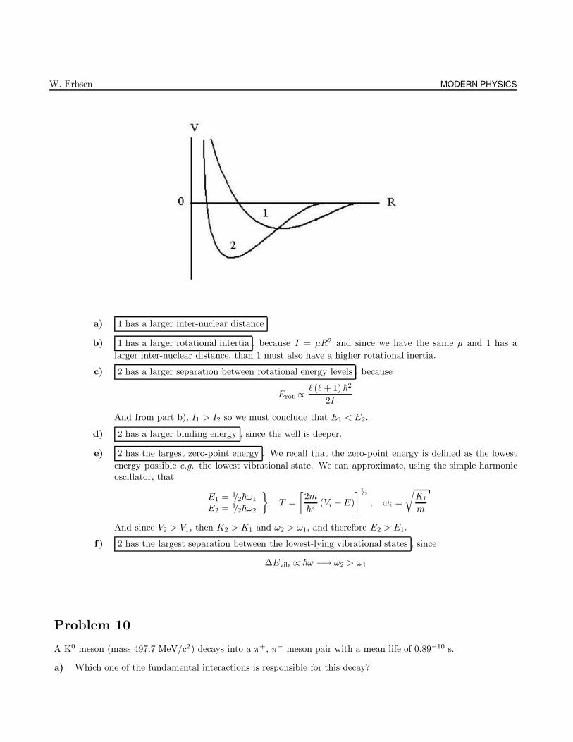
W. Erbsen MODERN PHYSICS
a) 1 has a larger inter-nuclear distance
b) 1 has a larger rotational intertia , because I = µR2 and since we have the same µ and 1 has a
larger inter-nuclear distance, than 1 must also have a higher rotational inertia.
c) 2 has a larger separation between rotational energy levels , because
Erot ∝` (` + 1) ~2
2I
And from part b), I1 > I2 so we must conclude that E1 < E2.
d) 2 has a larger binding energy , since the well is deeper.
e) 2 has the largest zero-point energy . We recall that the zero-point energy is defined as the lowest
energy possible e.g. the lowest vibrational state. We can approximate, using the simple harmonicoscillator, that
E1 = 1/2~ω1
E2 = 1/2~ω2
T =
[2m
~2(Vi −E)
]1/2
, ωi =
√Ki
m
And since V2 > V1, then K2 > K1 and ω2 > ω1, and therefore E2 > E1.
f ) 2 has the largest separation between the lowest-lying vibrational states , since
∆Evib ∝ ~ω −→ ω2 > ω1
Problem 10
A K0 meson (mass 497.7 MeV/c2) decays into a π+, π− meson pair with a mean life of 0.89−10 s.
a) Which one of the fundamental interactions is responsible for this decay?
CHAPTER 5: DEPARTMENTAL EXAMINATIONS 463
b) Suppose the K0 has a kinetic energy of 276 MeV when it decays, and that the two π Mesons emerge at equalangles to the original K0 direction. Find the kinetic energy of each π meson and the opening angle betweenthem. The mass of a π meson is 139.6 MeV/c2.
Solution
a) This decay is caused by the weak interaction . This is know because Ko has strange quarks, while
π-particles do not. Only in the weak interaction strangeness is not conserved.
b) At this point, we must employ the wonders of conservation of momentum, which says
pk = pπ+ + pπ− (5.3.54)
We now recall the handy formula
p2c2 = E2 −(mc2
)2(5.3.55)
First it would be nice to combine the two momenta from the Pions in (5.3.54):
pk = 2pπ (5.3.56)
However, we must be careful! The Pions do not both go in the same directions – they fly off atequal angles. Therefore, the momentum we concern ourselves with from with is
pk = 2pπ cos θ (5.3.57)
At this point we recognize that pπ in (5.3.57) can be rewritten using our good ol pal (5.3.55):
p2πc
2 = E2π −
(mπc
2)2 −→ pπc =
√E2
π − (mπc2)2
(5.3.58)
Now multiplying both sides of (5.3.58) by c,
pkc = 2pπc cos θ (5.3.59)
And substituting (5.3.58) into (5.3.59),
pkc = 2
√E2
π − (mπc2)2
cos θ (5.3.60)
And squaring both sides,
p2kc
2 = 4[E2
π −(mπc
2)2]
cos2 θ (5.3.61)
And substituting (5.3.55) into (5.3.61) for the LHS,
E2k −
(mkc
2)2
= 4 cos2 θ[E2
π −(mπc
2)2]
(5.3.62)
We know all the constants in this equation, except for Eπ . From conservation of energy,
Ek = 2Eπ −→ Eπ = 1/2Ek
Substituting this back into (5.3.65),
E2k −
(mkc
2)2
=4 cos2 θ
[E2
k
4−(mπc
2)2]
W. Erbsen MODERN PHYSICS
=cos2 θ[E2
k −(2mπc
2)2]
(5.3.63)
We can now solve (5.3.63) for θ,
θ = cos−1
[√E2
k − (mkc2)2
E2k − (2mπc2)
2
](5.3.64)
Before we go any further, we must recognize that Ek represents that total energy of the Ko, so itincludes both the mass energy term and the kinetic term. Using all the constants applied, (5.3.64)becomes
θ = cos−1
[√(497.7 + 276 MeV)
2 − (497.7 MeV)2
(497.7 + 276 MeV)2 − (2 · 139.6 MeV)
2
](5.3.65)
Evaluating (5.3.65), we are left with
θ = 34.82o
HOWEVER, if we want the total angle between the two Pions, we must double this result, whichyields
θ = 69.34o
The kinetic energy can just be found via Conservation of Energy, which says that
Tk = 2Tπ −→ Tπ =Tk
2−→ Tπ =
276 eV
2−→ Tπ = 138 MeV
Problem 11
A beam of 50 eV electrons is scattered from a cubic crystal with 1.2A spacing between the crystal planes. Theelectron beam is perpendicular to the crystal plane. At what angle will the first diffraction maximum be detected?
Solution
We first recall that the deBroglie wavelength is given by
λ =h
p(5.3.66)
And the momentum is
T =p2
2m−→ p =
√2mT (5.3.67)
Substituting (5.3.67) into (5.3.66) yields
CHAPTER 5: DEPARTMENTAL EXAMINATIONS 465
λ =h√
2mT(5.3.68)
We also recall that the equation for diffraction from a 3D period structure is
nλ = 2d sin θ (5.3.69)
Where we recognize that the path length must be in integer multiples of λ for completely constructiveinterference. For the first maxima, we have n = 1, and with (5.3.68), we have
h√2mT
= 2d sin θ −→ θ = sin−1
[h
2d
1√2mT
](5.3.70)
Substituting in the appropriate values into (5.3.70) yields
θ = sin−1
6.626× 10⁻³⁴ J · s
2 (1.2× 10⁻¹⁰ m)
1√2 (9.109× 10⁻³¹ Kg) (50 eV)
(1.602× 10⁻¹⁹ J · eV−1
)
−→ θ = 46.3o
Problem 12
One of the strongest emission lines observed from distant galaxies comes from Hydrogen and has a wavelength of122 nm (in the ultraviolet region).
a) How fast must a galaxy be moving away from us in order for that line to be observed in the visible region of366 nm?
b) What would be the wavelength of the line if that galaxy were moving towards us at the same speed?
Solution
a) If the source and receiver are moving away from each other, the Doppler effect says that
f ′ =
√1 − u2/c2√1 + u2/c2
fo
=
√1 − u2/c2
1 + u2/c2fo
(5.3.71)
Recalling that f = c/λ, we can rewrite (5.3.71) in the following form
1
λ′=
√1 − u/c
1 + u/c
1
λo
W. Erbsen MODERN PHYSICS
(λo
λ′
)2
=1 − u/c
1 + u/c(5.3.72)
=[1 − u/c]
[1 + u/c]
(c/c)
(c/c)
=c − u
c + u(5.3.73)
So, with (5.3.73) and the values given, we have
c− u
c+ u=
(λ0
λ′
)2
=
(122 nm
366 nm
)2
=
(1
3
)2
=1
9(5.3.74)
Rewriting, (5.3.74) becomes
c− u
c+ u=
1
9
9 (c− µ) =c+ u
9c− 9u =c+ u
u+ 9u =9c− c
From which it is easy to see that
u =8
10c
b) If the galaxy is moving towards Earth at the same speed, we simply change the sign of u in (5.3.72):
1
λ′=
√1 + u/c
1 − u/c
1
λ0
λ′ =
√1 − u/c
1 + u/cλ0
=
√1 − 0.8
1 + 0.8122 nm
=122 nm
3
Which finally leads us to
λ′ = 40.67 nm
Problem 13
Hall effect: Consider a free electron gas with an electric field E along the x-direction. The electrons are con-stantly undergoing collisions resulting in some average velocity E is applied.
a) The conductivity is defined using the current density j = Eσ. Find an expression for σ in terms of therelaxation time T which is half of the time between successive collisions. Let n be the density of electrons in
CHAPTER 5: DEPARTMENTAL EXAMINATIONS 467
the material and m the electron mass.
b) Now assume the electron gas is confined to a wire lying along the x-direction (E is still applied). Under thesecircumstances the equation of motion of an electron is
mdv
dt= −e (E + v × B) −m
v
T(5.3.75)
Where the first term in the Lorentz force and the second term takes account of collisions. It is found thata voltage develops along the y-direction (across the wire). A measure of this voltage is given by the Hallconstant R = Ey/(j ·Bz). Show that R = −1/(ne).
c) Will the Hall constant be larger in a metal or a semiconductor and why?
Solution
a) To find an expression for the conductivity, σ in terms of the relaxation time, T , we must employseveral not-so-tedius substitutions. First, we write down the (given) Ohm’s Law:
J = σE (5.3.76)
We also recall that the drift velocity is defined by
v =J
nq(5.3.77)
Where v is the velocity vector. We also recall that
v = a · T (5.3.78)
Where a is the acceleration of course. Now, from Newton’s second law,
F = ma (5.3.79)
And we must also recall that the force on a charged particle is given by
F = −qE (5.3.80)
Setting (5.3.79) equal to (5.3.80),
ma = −qE −→ a = −qEm
(5.3.81)
We now take (5.3.81) and substitute it back into (5.3.78):
v =
(−qEm
)· T (5.3.82)
We now set (5.3.82) equal to (5.3.77), which yields
J
nq= −qE
m· T −→ J =
nq2ET
m(5.3.83)
And finally, we set (5.3.83) and (5.3.83) equal to one another:
W. Erbsen MODERN PHYSICS
σE =nq2ET
m−→ σ =
nq2T
m(5.3.84)
b) The very first thing we need to do in this problem is to solve (5.3.75), which reads (for convienence)
mdv
dt= −q (E + v × B) − mv
T(5.3.85)
Let’s evaluate the cross product first. We are told that the magnetic field is along the z-direction,and so
v × B =i j zvx vy vz
0 0 Bz
= vyBz i − vxBz j (5.3.86)
Substituting this in to (5.3.85) and breaking down the components,
md(vx + vy + vz)
dt= −q
(Ex + Ey +Ez + vyBz i− vxBz j
)− m(vx + vy + vz)
T(5.3.87)
A voltage only exists along the y-direction, so lets get rid of everything not in the y-direction, and(5.3.88) becomes
mdvy
dt= −q
(Ey − vxBz j
)− mvy
T
And now,
0 = −q(Ey − vxBz j
)−→ vx = −Ey
Bzj (5.3.88)
Recalling that J · R = vx, (5.3.88) becomes
R =Ey
JBzj (5.3.89)
And now, recall that
J ·R = vx, J = q · v · n
Combining these,
Rqvxn = −vx −→ R = − 1
nq(5.3.90)
c) The hall constant will be larger .
Problem 14
The density of states g(E) is defined as the number of electronic states per unit energy range.
CHAPTER 5: DEPARTMENTAL EXAMINATIONS 469
a) Write down an expression for the density of the electron states in metal.
b) Find an expression for the Fermi energy from a).
c) Find an expression for the fraction of the conduction electrons which are within kT of the Fermi energy.
d) Evaluate this fraction for Copper at T = 300K. [Copper is a monovalent metal with ρ = 8.92g/cm3 andatomic weight M = 63.5g/mole.]
Solution
a) In order to find an expression for the density of states for a 3D electron gas, we start with theassumption that the metal is in the shape of a cube, each side having a length of L. Assumingfor the time being hat we have one free electron and infinite potential at the cube boundaries, theEigenenergies are given by
E =~2π2
2mL2
[n2
x + n2y + n2
z
](5.3.91)
For macroscopic systems, we assume that L is large enough that we can assume that the energyspectrum is continuous. In this approximation, the total number of states (up to an energy E)
is proportional to the volume of a sphere of radius r =[n2
x + n2y + n2
z
]1/2. Since we are only
interested in one quadrant, we concern ourselves with only 1/8th of the total volume of the sphere.Furthermore, we also have a 2-fold degeneracy, so we must also include a factor of 2. So, we have
N =2 · 1
8· 4
3π[n2
x + n2y + n2
z
]2/2
=π
3
[n2
x + n2y + n2
z
]3/2(5.3.92)
From (5.3.91) we have
[n2
x + n2y + n2
z
]=
2mL2
~2π2E (5.3.93)
Substituting (5.3.93) into (5.3.92),
N =π
3
[2mL2
~2π2E
]3/2
(5.3.94)
Recalling that the density of states is defined by
g(E) =dN
dE(5.3.95)
We then substitute (5.3.94) into (5.3.95), yielding
g(E) =d
dE
[π
3
[2mL2
~2π2E
]3/2]
=(2m)
3/2 L3
3~3π2
d
dE
[E
3/2]
=(2m)
3/2 L3
3~3π2
[3
2E
1/2
](5.3.96)
W. Erbsen MODERN PHYSICS
Simplifying, (5.3.96) leads us to
g(E) =(2m)
3/2 L3
2~3π2E
1/2 (5.3.97)
b) We first recall that the number of particles in a system is given by
N =
∫ EF
0
g(E) · f(E) dE (5.3.98)
Where g(E) is the density of states, and f(E) is the relevant distribution function, which in ourcase is the Fermi-Dirac function:
f(E) =1
exp [(E − µ)/kBT ] + 1(5.3.99)
For T = 0, this distribution gives the average number of particles in a state of energy E to be 1 forE < µ and 0 for E > µ. This maximum occupied energy (µ(T = 0)) is known as the Fermi Energy.
So, letting f(E) → 1, and substituting (5.3.97) into (5.3.98), we have
N =
∫ EF
0
[(2m)
3/2 L3
2~3π2E
1/2
]dE
=(2m)
3/2 L3
2~3π2
∫ EF
0
E1/2dE
=(2m)
3/2 L3
2~3π2
[2
3E
3/2F
]
=(3m)
3/2 L3
2~3π2E
3/2F (5.3.100)
Solving (5.3.100) for EF ,
EF =
[3~3π2
(2m)3/2 L3
N
]2/3
Which can be rewritten slightly nicer as
EF =~2
2m
[3Nπ2
L3
]2/3
(5.3.101)
c) In order to find the fraction of conduction electrons within kBT of the conduction band, we needto make a few assumptions. First, we assume that the density of states is constant over the entirekBT band, and secondly that the Fermi-Dirac distribution is still on the order of 1 for particles inthis region. Then the number of particles within the kBT band is given by
NkBT =g(EF ) · kBT (5.3.102)
Substituting (5.3.97) into (5.3.102),
NkBT =
[(2m)
3/2 L3
2~3π2E
1/2
]· kBT (5.3.103)
CHAPTER 5: DEPARTMENTAL EXAMINATIONS 471
And also from (5.3.94) we know that
N =π
3
[2mL2
~2π2E
]3/2
(5.3.104)
Taking the ratio of (5.3.103) and (5.3.104) leads us to
NkBT
N=
3
2
1
EFkBT (5.3.105)
d) We now wish to evaluate (5.3.105) for Copper. The first thing that we want to do is find the fractionN/V , which is:
N
V=
8.92 mol
63.5 cm3·(
100 cm
1 m
)3
· 6.022× 1023 atoms
mol(5.3.106)
The Fermi Energy as found in (5.3.101) is
EF =
[3~3π2
(2m)3/2 L3
N
]2/3
=
[3~3π2
(2m)3/2
] 2/3 [N
V
]2/3
(5.3.107)
Where I have set L3 → V . Substituting (5.3.107) into (5.3.105),
NkBT
N=
3
2kBT
[
3~3π2
(2m)3/2
]2/3 [N
V
]2/3
−1
=3
2kBT
[
(2m)3/2
3~3π2
]2/3 [V
N
]2/3
(5.3.108)
Substituting in to (5.3.108) the appropriate values,
NkBT
N=
3
2
(1.381× 10⁻²³ J ·K−1
)(300 K)
(2 · 9.109× 10−31 Kg
)2/3
3 · 1.055× 10−34 J · s
2/3
·[
63.5
8.92 · 103 · 6.022× 1023
]2/3
Evaluating this, we are left with
NkBT
N= 5.5 × 10⁻³
Problem 15
A hypothetical atom has only two excited states, at 4.0 and 7.0eV, and has a ground-state ionization energy

W. Erbsen MODERN PHYSICS
of 9.0eV. If we used a vapor of such atoms from the Franck-Hertz experiment, for what voltages would we expectto see decreases in the current? List all voltages up to 20V.
Solution
We first recall the principles behind the Franck-Hertz experiment. This seminal experiment demonstratedthe quantization of atomic energy states by means of accelerating negatively charged electrons through apositively charged grid, surrounded by Mercury vapor. The resulting data takes the form of an increasesoscillating signal, when plotting the net electron current vs the potential difference of the grid.
The hypothetical atom described in the prompt has three energy levels:
V3 =9 eV [Continuum]
V2 =7 eV
V1 =4 eV
The electron current will drop whenever any multiple of V1, V2, or V3 is reached. Therefore,
1V1 =4 eV
2V1 =8 eV
3V1 =12 eV
4V1 =16 eV
5V1 =20 eV
1V2 =7 eV
2V2 =14 eV
1V3 =9 eV
2V3 =18 eV
Also, allowing for combinations of V1, V2 and V3,
V1 + V2 =11 eV
V1 + V3 =13 eV
V2 + V3 =16 eV
2V1 + V2 =15 eV
2V1 + V3 =17 eV
3V1 + V2 =19 eV
So, we expect the current to drop at the following values:
V = 4, 7, 8, 9, 11, 12, 13, 14, 15, 16, 17, 18, 19, and 20 eV
Problem 16
CHAPTER 5: DEPARTMENTAL EXAMINATIONS 473
Consider two protons of mass mp and electric charge e, separated by a distance r.
a) Compute the ratio of the electromagnetic to gravitational forces acting on the protons.
b) Given your every day experiences with bulk neutral bodies, what do you conclude from the numerical valuesthat you computed in a)? In particular, what force is more important for small bodies? For very large bodies?
c) Consider a large spherical body, of constant density, made up of N hydrogen atoms. Determine the criticalmass of this body at which the binding energy of the body just balances the gravitational potential energyof teh body. Use the fact that the atom size is approximately the Bohr radius [= 1/(ame)] and the atomicbinding energy is twice the Rydberg energy [=a2me/2], where a is the fine structure constant and me is theelectron mass. Also assume that the mass of the hydrogen atom is equal to mp.
d) Determine the critical radius of the body, corresponding to the critical mass derived in c).
Solution
a) The electrostatic force between the two protons is
Fe =1
4πε0
e2
r2⇒ K
e2
r2(5.3.109)
While the gravitational force acting on the bodies is
FG = GM2
p
r2(5.3.110)
So that if we were to find the ratio of electromagnetic and gravitational forces acting on the protons,we would divide (5.3.109) by (5.3.110), which leads us to
Fe
Fg=Ke2/r2
Gm2p/r
2=
Ke2
Gm2p
(5.3.111)
Plugging into (5.3.111) the appropriate values,
Fe
Fg=
(8.988× 10⁹ N · m2 · C−2
) (1.6022× 10⁻¹⁹ C
)2(6.674× 10⁻¹¹ N ·m2 Kg−2
)(1.673× 10⁻²⁷ Kg)
2 −→ Fe
Fg≈ 1036 (5.3.112)
b) Rewriting (5.3.111),
Fe
Fg=K
g
(e
mp
)2
≈1020
(e
mp
)2
(5.3.113)
So, unless the mass of the particle is more than ten orders of magnitude larger than the charge, theelectrostatic force will be more prevalent.
However, in our everyday experiences, we have mostly bulk substances, being neutral in nature,so for really large objects (stars, planets, etc), the gravitational force wins, whereas on the atomiclevel (atoms, molecules), the electrostatic force still dominates.
W. Erbsen MODERN PHYSICS
c) Here we must find the critical mass, in which the binding energy just balances the gravitationalenergy. In the following calculations, we will assume that the Hydrogen atom radius is on the orderof the Bohr radius, and that the binding energy of Hydrogen is twice the Rydberg energy. We firstrecall that
ρ =m
V−→ m = V · ρ =
4
3πr3ρ (5.3.114)
Taking the differential limit of (5.3.114),
dm = 4πr2ρ dr (5.3.115)
We also recall that the gravitational self energy, in differential form is
Ug = −GMr
dm (5.3.116)
Substituting (5.3.115) into (5.3.116) and carrying out the integration,
Ug = −∫ R
0
Gm
rdm
= −∫ R
0
G
r
(4
3πr3ρ
) (4πr2ρ dr
)
= − 16π2G
3ρ2
∫ R
0
r4 dr
= − 16π2G
3ρ2
[R5
5
]
= − 16π2Gρ2
15R5 (5.3.117)
And the density is (recall that M = mpN):
ρ =M
4/3πR3=
3mpN
4πR3(5.3.118)
And according to the prompt, the binding energy of one Hydrogen atom is
Ub =
(a2m1
2
)2 (5.3.119)
For the entire mass, (5.3.119) becomes
Ub = NA2me (5.3.120)
Putting (5.3.118) into (5.3.117),
UG = − 16π2GR5
15·9m2
pN2
16π2R6
= −G9m2
pR5N2
15R
= −G9m2
pN2
15R
= −G3m2
pN2
5R
CHAPTER 5: DEPARTMENTAL EXAMINATIONS 475
= − 3
5Gm2
p
RN2 (5.3.121)
Recalling now that
Ub = Na2me (5.3.122)
Setting (5.3.121) and (5.3.122) equal to one another,
Na2me =3
5Gm2
p
RN2
mpN =5
3
a2me
GmpR (5.3.123)
We now recall that M = mp ·N , so that (5.3.123) becomes
M =5
3
a2me
GmpR (5.3.124)
d) The critical radius is related to the critical mass as∗
R = N1/3RBohr
Applying this to (5.3.124), we are left with†
R =
[5
3
a2me
Gm2p
R2Bohr
]1/3
Problem 17
Use the Bohr theory to answer the following question:
a) Derive the energy levels of the hydrogen atom.
b) The orbiting speed of the electron in the ground state.
c) If an excitation laser pulse has a duration of one picosecond, what is the principal quantum number n forwhich the orbiting period of the electron is about one picosecond?
d) If the electron is replaced by a negatively charged muon, what is the ground state energy of this muon? Usethese facts to get your numerical answers: the ground state of atomic hydrogen has a binding energy of 13.6eV, the mass of the proton is 1837 times that of en electron and teh mass of a muon is 206 times that of anelectron. What is the photon energy for the n = 2 to n = 1 transition in this case?
e) Use the uncertainty principle to estimate the ground state energy of atomic hydrogen and compare the resultsfrom the Bohr model.
∗Hint: volume of sphere = N · volume of hydrogen.
†R = N1/3 r0
W. Erbsen MODERN PHYSICS
Solution
a) The potential (energy) of a Hydrogen atom is given in its most general form by
V = − 1
4πε0
e2
r(5.3.125)
While the total energy of the system (kinetic plus potential) is
E =T + V
=mev
2
2− 1
4πε0
e2
r(5.3.126)
Assuming that we have a circular orbit, we may use the following formula for centripetal force:
F =mv2
r=
1
4πε0
e2
r2︸ ︷︷ ︸Coulomb Force
(5.3.127)
Solving (5.3.127) for v2,
v2 =1
4πε0
e2
mer(5.3.128)
And now substituting (5.3.128) back into (5.3.126),
E =me
2
(1
4πε0
e2
mer
)− 1
4πε0
e2
r
=1
2
(1
4πε0
e2
r
)− 2
2
(1
4πε0
e2
r
)
= − 1
8πε0
e2
r(5.3.129)
One of Bohr’s key assumptions is that circular orbit had quantized angular momentum. Mathe-matically,
L = mvr = n~ (5.3.130)
Solving (5.3.130) for r,
r =n~
mev−→ r2 =
n2~2
m2ev
2(5.3.131)
Substituting our value for v2 from (5.3.128) back into (5.3.131), we have
r2 =n2~2
m2e
4πε0mer
e2
r =n2~24πε0mee2
(5.3.132)
Now substituting (5.3.132) into (5.3.129),
E = − 1
8πε0e2 · mee
2
n2~24πε0(5.3.133)
CHAPTER 5: DEPARTMENTAL EXAMINATIONS 477
We can rearrange (5.3.133), which finally leads us to
E = − mee4
2 (4πε0)2n2~2
(5.3.134)
b) For the ground state, n = 1, and using (5.3.128), and (5.3.132), we have
v =
[1
4πε0
e2
me
mee2
~24πε0
]1/2
=
[1
(4πε0)2
e4
~2
] 1/2
=1
4πε0
e2
~(5.3.135)
Plugging in the appropriate values into (5.3.135),
v =(98.987× 10⁹ N · m2 · C−2
) (1.6023× 10⁻¹⁹ C)2
(1.055× 10⁻³⁴ J · s) −→ v = 2.187× 10⁶ m · s−1 (5.3.136)
c) By default, the orbital period is given by
Tn =2πrn
vn(5.3.137)
Substituting our previous functional value of v into (5.3.137), as well as our value for r and also(5.3.137), we have
Tn =2π
(n2~24πε0mee2
)(4πε0 ·
n~
e2
)
=2π (4πε0)
2n3~3
mee4(5.3.138)
Solving (5.3.138) for n,
n =
(Tnmee
4
2π (4πε0)3
~3
)1/3
=
(Tnmee
4K2
2π~3
) 1/3
(5.3.139)
Substituting in the appropriate values into (5.3.139),
n =
((10−12 s
) (9.109× 10⁻³¹ Kg
) (1.602× 10⁻¹⁹ C
)4 (8.987× 10⁹ N ·m2 · Kg−2
)
2π (1.055× 10⁻³⁴ J · s)3
)(5.3.140)
Evaluating (5.3.144), we are left with,
n = 18.73 −→ n = 19
d) The energy of a Muon instead of an electron is found by replacing me in (5.3.136) by µ, which isthe reduced mass of the atom, and is mathematically described by
W. Erbsen MODERN PHYSICS
µ =mp ·mµ
mp +mµ(5.3.141)
The relative mass of a proton to an electron is mp = 1838 me, so (5.3.141) becomes
µ =(1836 me) (207 me)
1836 me + 207 me= 186.0 me (5.3.142)
With this new value of reduced mass, we must re-evaluate our results from (5.3.134), which leadsus to
E = − mee4
2n2~2k2
= −(9.109× 10⁻³¹ Kg
) (1.602× 10⁻¹⁹ C
)4 (8.897× 10⁹ N · m2 · Kg−2
)
2n2 (1.055× 10⁻³⁴; J · s)2
=−13.6 eV
n2(5.3.143)
Applying our reduced mass from (5.3.145) to (5.3.146),
E =−14.6 eVPn2 186.0 me
me
=−13.6 eV · 186.0
n2(5.3.144)
For the ground state, (5.3.144) becomes
Egs(µ) = 2629 eV (5.3.145)
And the photon energy for this case would just be E2 − E1 evaluated using (5.3.144), which yields
∆E = E2 −E1 = −2529 eV
(1
4− 1
)−→ ∆E = 1896 eV
e) From the uncertainty relation, we recall that
∆p∆r ∼ ~ −→ ∆p ∼ ~
∆r
Using these results, the total energy is
E =p2
2m− k
e2
r
=~2
2m (∆r)2 − ke2
r(5.3.146)
We must minimize (5.3.146) in the usual fashion,
∂E(r)
∂r=0
~2
2m
∂
∂r
1
r2− ke2
∂
∂r
1
r=0
(5.3.147)
Rearranging things a bit, (5.3.147) becomes
CHAPTER 5: DEPARTMENTAL EXAMINATIONS 479
r =~2
2m· 2 · 1
Ke2
=~2
kme2(5.3.148)
Substituting (5.3.148) back in to (5.3.146),
E =~2
2m
(K2m2e4
~4
)− ke2
(Kme2
~2
)
=me4k2
2~2− me4k2
~2
=me4k2
~2(5.3.149)
From (5.3.149), we can easily deduce that
E =me4
2~2k2 (5.3.150)
Which we can see is identical to (5.3.144).
Problem 18
The resistivity ρ of a metal due to scattering of the quasi-free electrons as per the Drude model is given by
ρ =mevav
ne2λ(5.3.151)
a) Derive the expression above. What are the quantities n and λ, and explain qualitatively is ρ inverselyproportional to them?
b) The average electron velocity vav is very different in the classical and quantum-mechanical treatments. Ex-plain the origin of the difference (why the quantum-mechanical velocity is much larger at room temperature,and is nearly independent of temperature).
c) How is λ related to the cross-section σ for scattering of conduction electrons in the metal?
d) Naively, one might take σ to be the geometrical area of the lattice ions. A more correct treatment gives amuch smaller cross section which depends on temperature. Explain how this arises.
Solution
a) We first note that n is the number of electrons per unit volume, while λ is the mean free path. Theelectrons will move with a drift velocity, vd. In some time interval ∆t all charge that passes throughcross sectional area A will be ∆Q = neAvd∆t. We can find the current by taking the derivative,
I =dQ(t)
dt=
d
dt[neAvd∆t] (5.3.152)
W. Erbsen MODERN PHYSICS
If we assume that the time interval is appropriately constant, (5.3.152) becomes
I = neAvd (5.3.153)
At this point, we must recall a number of seemingly arbitrary definitions. We of course recall Ohm’slaw as V = IR, and the resistivity is given as
R =ρL
A(5.3.154)
We also recall that the electric field within the material is given by
E =V
L−→ V = EL (5.3.155)
Substituting (5.3.155) into Ohm’s Law, we have
EL = IR (5.3.156)
We now substitute our expression for resistivity from (5.3.154) into (5.3.156),
EL = I
(ρL
A
)−→ I =
EA
ρ(5.3.157)
We now set (5.3.153) equal to (5.3.157),
neAvd =EA
ρ−→ ρ =
E
nevd(5.3.158)
In the same mantra as before, we recall that Newton’s second law says F = ma, F = eE, andv = aτ , so we can solve for v and arrive at
vd =eEτ
m(5.3.159)
Putting (5.3.159) back into (5.3.158),
ρ =E
ne· m
eEτ−→ ρ =
m
ne2τ(5.3.160)
But hold on there jack, τ is really the average time the particle goes without a collision, and wewant our expression in terms of the mean free path. The formula which connects these two entitiesis simple: τ = λ/vavg. Substituting this back into (5.3.160),
ρ =m
ne2· vavg
λ−→ ρ =
mvavg
ne2λ(5.3.161)
b) The average electron velocity, vavg is a very different animal when investigated in either the classicalor quantum-mechanical regime. Classically,
T =mv2
2=
3
2kBT (5.3.162)
Playing with (5.3.162) a little bit,
v =
√3kBT
m(5.3.163)
Quantum-mechanically, only electrons that have energies within the kBT band contribute, so theaverage energy is the Fermi energy: Eavg = EF :
CHAPTER 5: DEPARTMENTAL EXAMINATIONS 481
T = EF =mv2
2(5.3.164)
Playing some more,
vavg =
√2EF
m(5.3.165)
Where we note that EF does not depend on T , so vavg does not depend on it either. Freaky! Aqualitative summary,
Ef = kBTF kBTroom −→ vavg(Quantum) vavg(Classical)
c) To answer this we need only consider two elements. Firstly, we recognize that an electron enteringon the left of the cylinder will be scattered before it reaches the right side of the same cylinder. Weknow that the volume of the cylinder is λσ, and that the density of scatterers is n = 1/λσ, so, ouranswer is then
λ =1
nσ
d) The area swept out by the atomic vibrations perpendicular to the direction of propagating electronsis given by the cross section, σ. Increasing the temperature, T increases the vibrations. Therefore,
as they both increase without limit, we have no choice but to say that σ, T → ∞ at the same rate.
Problem 19
The band theory of solids can be used to explain how a pure, intrinsic semiconductor (such as germanium)can become a p-type semiconductor.
a) How do conduction bands arise in a solid?
b) Sketch an energy level diagram for electrons in a pure germanium crystal. Indicate both the conduction andvalence bands and give order of magnitude estimates of the energies in your diagram.
Solution
a) This is a tricky question to answer, in the sense that the full explanation is a science in and ofitself. Irregardless, we start with the idealized scenario of a repeating series of potentials (a “DiracComb”) that has a fixed height (V0) and each barrier is a fixed distance from one another a. TheBarrier itself has a width, which we call b. These series of potentials go on forever, as to neglectany edging effects.
At this point, we introduce our old friend the TISE in 1-D:(− ~2
2m
∂
∂x+ V (x)
)ψ(x) = Eψ(x) (5.3.166)
Whose realizable solutions end up begin
W. Erbsen MODERN PHYSICS
ψ(x) = Aeikx , k =
√2m (E − V (x))
~(5.3.167)
Our periodicity boundary condition also satisfies the TISE, but the solution will be shifted by somephase factor:
ψ (x+N(a+ b)) = eik(a+b)ψ(x) (5.3.168)
Where (5.3.168) is lovingly referred to Bloch’s Theorem. Solving the TISE for repeating latticesusing boundary conditions (eventually yields a transcidental equation, which can be used to visuallydetermine the bands and band-gaps within a particular solid.
The size, length, and location of the bands and bandgaps depends on the distance between thepotentials, a, the width of the potentials, b, and the height of the potentials, V0. From these threevariables, we can plot the energy versus the wave number, and depending on the combination ofthe supplied variables, the plots may indicate a conductor, insulator, or a semiconductor.
For a conductor, the Fermi Energy lies within a band and accordingly, the valence bands andconduction bands overlap. This implies that at T = 0, some of the electrons will be “free” to“conduct.”
For an insulator, the Fermi energy lies either at the beginning, or the end of the gap (orsomewhere inbetween). Subsequently, at T = 0 all orbitals below EF are filled, leaving no ”free“electrons to “conduct.”
For the case of a semi-conductor, the gaps are small enough for some electrons to jump acrossand become free. These particular characteristics can be controlled by way of introducing impuritiesto the pure semiconductor (known as “doping”).
b) I can’t sketch here, but it should be fairly straightforward. Anyway, as far as an order of magnitudeestimate for the gap spacing between the valence and conduction bands in a semi-conductor, the only
way I can think to solve this problem is by experience, which tells me that the gap should be ∼ 1 eV
Problem 20
When sodium metal is illuminated with light of wavelength 4.20 × 10² nm, the stopping potential is found tobe 0.64 V; when the wavelength is changed to 3.10 × 10² nm, the stopping potential becomes 1.69 V. Using only
this data and the values of the speed of light and electronic charge, find the work function of sodium and the valueof Planck’s constant.
Solution
We first recall that the key equation for the photoelectric effect is
Emax = hf − φ (5.3.169)
The stopping potential is the potential that is required to stop an electron with some maximum kineticenergy Emax. Since the potential energy created by a potential difference V is U = qV , (5.3.169) becomes
qV =hf − φ
CHAPTER 5: DEPARTMENTAL EXAMINATIONS 483
=hc
λ− φ (5.3.170)
Given that λ = 4.20× 10² nm, and also that the stopping potential is V − 0.65 V, (5.3.170) becomes
qV1 =hc
λ1− φ
V1 = 0.65 Vλ1 = 420× 10−9 m
(5.3.171)
And similarly, for λ = 3.10× 10² nm and V = 1.69 V, we have
qV2 =hc
λ2− φ
V2 = 1.69 Vλ2 = 310× 10−9 m
(5.3.172)
Solving (5.3.171) and (5.3.172) for φ and setting them equal to one another leads us to
hc
λ1− qV1 =
hc
λ2− qV2
hc
(1
λ1− 1
λ2
)=q (V1 − V2)
h =q
c(V1 − V2)
(1
λ1− 1
λ2
)−1
(5.3.173)
Substituting in the correct values into (5.3.173) leads us to
h =1.602× 10⁻¹⁹ C
2.998× 10⁸ m · s−1(0.65 V − 1.69 V)
(1
420 × 10−9 m− 1
310 × 10−9 m
)−1
−→ h = 6.578× 10⁻³⁴ J · s (5.3.174)
Now, using either (5.3.171) or (5.3.172), we can calculate the work function φ. Using (5.3.172),
φ =hc
λ1− qV1
Substituting in the appropriate values,
φ =
(6.578× 10⁻³⁴ J · s
) (2.998× 10⁸ m · s−1
)
(420× 10−9 m)−→ φ = 3.661× 10⁻¹⁹ J
φ = 2.285 eV
Problem 21
Two identical photons are produced when a proton and an antiproton, both at rest, annihilate each other. Whatare the frequencies and corresponding wavelengths of the photons? Is it possible to produce a single photon inproton-antiproton annihilation? Why or why not?
Solution
W. Erbsen MODERN PHYSICS
We first recall the following energy/momentum relations:
E2p =m2c4 + p2c2 (5.3.175a)
E2p =m2c4 (5.3.175b)
We also recall that Ep = mc2 = 938.3 MeV. Now, recall from Einstein’s relation that
Eγ = hf −→ f =Eγ
h
=938.3× 10⁶ eV
4.136× 10⁻¹⁵ eV · s=2.296× 10²³ Hz (5.3.176)
Now, we can say that
λ =c
f=
3 × 10⁸ m · s−1
2.269× 10²³ Hz−→ λ = 1.322× 10⁻¹⁵ m
It is not possible to produce a single photon in this particular interaction, since it would violate con-
servation of momentum (recall that the protons start off at rest)
Problem 22
A dust particle at rest relative to the sun is in equilibrium between the radiation pressure and gravitationalattraction. What is the size of the dust particle? (For simplicity, you can assume that the dust particle inspherical)
Solution
We first recall that the radiation pressure is defined by
Prad =〈S〉c
(5.3.177)
Where 〈S〉 is the time-averaged Poynting vector, aka the intensity. The power emitted by the sun isaround P ≈ 3.8× 1026 W, and so the intensity is
I = 〈S〉 =3.8 × 1026 W
4πr2(5.3.178)
Applying (5.3.178) to (5.3.177),
Prad =3.8× 1026 W
4πr2c(5.3.179)
Since pressure is defined as P = F/A, then (5.3.179) becomes
CHAPTER 5: DEPARTMENTAL EXAMINATIONS 485
Frad =
(3.8× 1026 W
) (4πR2
)
4πr2
=
(3.8× 1026 W
)
r2R2 (5.3.180)
Now, if we assume that the dust particles are perfectly reflective, then (5.3.180) becomes
Frad =2
(3.8× 1026 W
)
r2R2 (5.3.181)
And we also recall that the gravitational force is given by
Fgrav = GmM
r2(5.3.182)
Equating (5.3.181) and (5.3.182),
2
(3.8× 1026 W
)
r2R2 = G
mM
r2
Solving for R, this becomes
R =
√GmM
2 (3.8× 1026 W)(5.3.183)
Problem 23
What is the density of a neutron star? Evaluate the size (radius) of a neutron star as massive as the sun,given that the radius 197
79 Au nucleus is 7 × 10⁻¹⁴ m, mass of the sun is 2 × 1030 kg.
Solution
Density is of course given by ρ = m/v, and given the supplied constants, we have
ρ =197 × 1.67× 10−27 Kg
4/3π (7 × 10⁻¹⁴ m)3
−→ ρ = 2.194× 10¹⁴ Kg ·m−3 (5.3.184)
To find the radius of the neutron star, we recall that from the density, we can say that
ρ =M
4/3πR3−→ R =
(3M
4πρ
)1/3
(5.3.185)
Plugging into (5.3.185) the appropriate values,
R =
((3)(2 × 1030 Kg
)
4π (2.194× 10¹⁴ Kg · m3)
)1/3
−→ R = 129589 m
W. Erbsen MODERN PHYSICS
Problem 24
A typical particle production process isp+ p −→ p+ p+ π0
where mp = 938MeV/c2, mass of π0 = 135MeV/c2.
a) In a standard accelerator one of the initial protons would be at rest. In this case what is the minimumlaboratory energy for the moving particle so that the reaction listed above occurs?
b) In colliding beam accelerators, such as the one proposed for the superconducting supercollider, the two initialparticles are moving towards each other with equal speeds. Why do colliding beam accelerators have anenergetic advantage over the type of accelerator from a)?
c) What energy would be required of each proton in a colliding beams accelerator to produce a pion?
Solution
We first recall the following:
E2 =p2c2 +(m0c
2)2
(5.3.186a)
E =mc2 (5.3.186b)
And that the invariant quantity is
(m0c
2)2
︸ ︷︷ ︸Lab frame invariant before collision
=
Center of mass frame invariant after collision︷ ︸︸ ︷E2 − p2c2 (5.3.187)
Where in the center of mass frame (COM) the momentum is zero, so (5.3.187) becomes
(m0c
2)2
= E2 (5.3.188)
Let’s make a table:
Before After• −→ • • → • → • →
Σm 2mp 2mp +mπ
(5.3.189)
a) If we choose not to use the COM frame, then the momentum is conserved (let’s do it this way). Wefirst apply conservation of energy to our system:
Ei = Ef (5.3.190)
Squaring (5.3.190) and substituting in (5.3.186a),
p2i c
2 +m2i c
4 = p2fc
2 +m2f c
4 (5.3.191)
Conservation of momentum says that pi = pf , and so (5.3.191) becomes
m2i c
4 =m2f c
4
CHAPTER 5: DEPARTMENTAL EXAMINATIONS 487
(2mpc
2)2
=[(2mp +mπ) c2
]2
4m2pc
4 =4m2pc
4 + 2mpmπc4 + 2mpmπc
4 +m2πc
4
0 =4mpmπc4 +m2
πc4
0 =mπc2
(mπc
2
2mpc2+ 2
)
0 =mπc2
(mπ
2mp+ 2
)(5.3.192)
We can now say that this is the threshold energy, which is the minimum possible energy that willallow this reaction to happen. The RHS of (5.3.192) is this so-called threshold energy:
ET = mπc2
(mπc
2
2mpc2+ 2
)
Substituting in the appropriate values, we have
ET = 135 MeV
(135 MeV
2 · 938 MeV+ 1
)−→ ET = 279.7 MeV (5.3.193)
And to find the total energy, we combine the results of (5.3.193) plus the rest mass energy of theproton:
Etot = 279.7 MeV + 938 MeV −→ Etot = 1217.7 MeV
b) Since in the case of a), all the energy needed to create the πo is carried by the first proton, howeverif both were to move towards one another, then the energy would need to be much less in order toreach the threshold energy.
c) If they are moving towards one another, we use the same logic as before - we want the threshold
energy, that is the energy that is just barely enough to complete the reaction. In this case, we careonly about the creation of three particles: two Protons, and one Pion. Therefore, each incidentproton must have an initial energy equal to
Ep =1
2(2mp +mπ)
Plugging in the appropriate number,
Ep =1
2[2 (938 MeV) + 135 MeV] −→ Ep = 1005.5 MeV
Problem 25
In a muonic hydrogen atom, the electron is replaced by a muon, which is 207 times heavier.
a) What is the wavelength of the n = 2 to n = 1 transition in Muonic hydrogen? In what region of theelectromagnetic spectrum does this wavelength belong?
b) How would the fine structure and Zeeman effects differ from those in ordinary atomic hydrogen?

W. Erbsen MODERN PHYSICS
Solution
a) We first recall the Rydberg formula, which reads
1
λ= R
(1
n2f
− 1
n2i
)(5.3.194)
While the Rydberg constant is given by
R =me
4πc~3
(e2
4πε0
)2
= 1.097× 10⁷ m−1 (5.3.195)
R ∼C ·me
Where me is the electron mass. For Muonic Hydrogen, we replace me with µ/me, where µ is thereduced mass, where
mµ = 207 me, mp = 1836 me
So, the reduced mass is
µ =(207 me) (1836 me)
(207 me) + (1836 me)= 186.0 me (5.3.196)
Substituting (5.3.196) into (5.3.194),
1
λ= R · µ
me
(1
n2f
− 1
n2i
)(5.3.197)
Substituting in the appropriate values, (5.3.197) becomes
1
λ=(1.097× 10⁷ m−1
)(186.0
me
me
)(1
4− 1
)
=1.530× 10⁹ m−1 (5.3.198)
From which it is easy to see that
λ = 6.535× 10⁻¹⁰ m
Which are x-rays.
b) The only appreciable difference between Hydrogen and Muonic Hydrogen is the difference in themasses of the electron and the Muon, respectively. Therefore, we must find the splitting as a func-tion of mass for both fine structure and Zeeman effects.
The fine structure is of order:
Efs ∼ α4me2 −→ Efs ∼m
While the Zeeman effect is of order:
Ez ∼me ·e~
2m· B −→ Ez ∼ 1
m

CHAPTER 5: DEPARTMENTAL EXAMINATIONS 489
Problem 26
For an intrinsic semiconductor, the number of electrons per unit volume in the conduction band and the numberof holes in the valence band are given by
n =NC exp
[−(EC − EF )
kBT
](5.3.199a)
p =NV exp
[−(EF −EV )
kBT
](5.3.199b)
Where
NC = NV =2(2πmkBT )
3/2
h3(5.3.200)
a) Find the position of the Fermi energy in an intrinsic semiconductor.
b) Show that the product of the number of electrons in the conduction band and the number of holes in thevalence band depends only on temperature and the gap energy, Eg.
c) Discuss how one can use the temperature (T ) dependence of the conductivity σ to approximately measurethe gap energy provided that T is not too high.
Solution
We first recall that the Fermi Energy is defined as the highest occupied state at T = 0 K. We also recallthat the Intrinsic Fermi Energy (Ei) is defined as the Fermi Energy in the absence of doping.
a) In an intrinsic semiconductor, the number of electrons is equal to the number of holes (n = p), sincethe thermal excitation of an electron leaves behind a hole in the valence band.
The very first thing that we wish to do is multiply (5.3.199a) and (5.3.199b):
np = NcNv exp
[−(Ec −Ev)
kBT
](5.3.201)
And furthermore, from (5.3.200), we may deduce that
NC = 2
(2πmekBT
h2
)3/2
(5.3.202a)
NV = 2
(2πmhkBT
h2
)3/2
(5.3.202b)
Where mh is the electron effective mass near the top of the valence band. Using (5.3.202a)-(5.3.202b), we can now rewrite (5.3.199a) and (5.3.199b), respectively:
n =2
(2πmekBT
h2
) 3/2
· exp
[−(Ec − EF )
kBT
](5.3.203a)
p =2
(2πmhkBT
h2
) 3/2
· exp
[−(EF − Ev)
kBT
](5.3.203b)
Multiplying (5.3.203a) and (5.3.203b) leads us to
W. Erbsen MODERN PHYSICS
np = 4
(2πkBT
h2
)3
(memh)3/2 exp
[−(Ec − Ev)
kBT
](5.3.204)
The intrinsic carrier concentration depends exponentially on (Ec −EV ) /2kBT .
At the Fermi Energy, n = p because the number of electrons and the number of holes are createdin pairs for intrinsic semiconductors, as is what we have here. So,
Nc exp
[−(Ec − Ef)
kBT
]=Nv exp
[−(EF − Ev)
kBT
]
Since Nc and Nv are equal in this case, this becomes
(Ec − Ef)
kBT= − (EF − Ev)
kBT
Ec − Ef = − EF − Ev
From which it is easy to gather that
EF =Ev +Ec
2
In other words, the Fermi Energy is located exactly inbetween the valence band and the conductionband.
b) From the results of the previous problem, we found that
np = 4
(2πkBT
h2
)3
(mhme)3/2 exp
[− Eg
kBT
](5.3.205)
Where Eg = Ec − Ev is the gap energy.
c) We recall from Ohm’s law that
σ =j
E, Vd =
j
nq
Combining these, we find that
σ =nqv
E(5.3.206)
Also recalling that F = qE, (5.3.206) becomes
σ =nq2v
F(5.3.207)
Now, we recall that v = aτ , where τ is the time between collisions. Combining this with Newton’ssecond law, F = ma, we have F = vm/τ , and (5.3.207) becomes
σ =nq2τ
m(5.3.208)
Recalling from before that
σ =σc + σv
CHAPTER 5: DEPARTMENTAL EXAMINATIONS 491
=q2τ
m
2
(2πmekBT
h2
) 3/2
· exp
[−(Ec − EF )
kBT
]+ 2
(2πmhkBT
h2
) 3/2
· exp
[−(EF − Ev)
kBT
]
From this we can easily say that
σ ∼ C exp
[−(Ev +Ec)
kBT
]
So, as long as the temperature is low, the gap will dominate this equation, and we can solve for thegap as needed.
Problem 27
The potential energy between two atoms in a molecule can often be described rather well by the Lennard-Jonespotential, which can be written
U(r) = U0
[(ar
)12
− 2(ar
)6]
(5.3.209)
Where U0 and a are constants.
a) Find the interatomic separation r0 in terms of a for which the potential energy is minimum.
b) Find the corresponding value of Umin.
c) Use the figure below to obtain numerical values for r0 and U0 for the H2 molecule. Express your answer innanometers and electron volts.
d) Make a plot of the potential energy U(r) versus the internuclear separation r for the H2 molecules. Plot eachterm separately, together with the total U(r).
Solution
a) To find the value of the interatomic separation r0 when the potential energy is at a minimum, wemust minimize (5.3.209). The general prescription for minimizing any function is to take the deriva-tive with respect to the minimization variable and set it equal to zero, solving for the appropriateminimized value. In our case,
∂U(r)
∂r
∣∣∣∣r=r0
= 0 (5.3.210)
So, applying (5.3.210) to (5.3.209), we have
∂
∂r
[(ar
)12
− 2(ar
)6]
= 0
a12
[∂
∂r
1
r12
]− 2a6
[∂
∂r
1
r6
]= 0
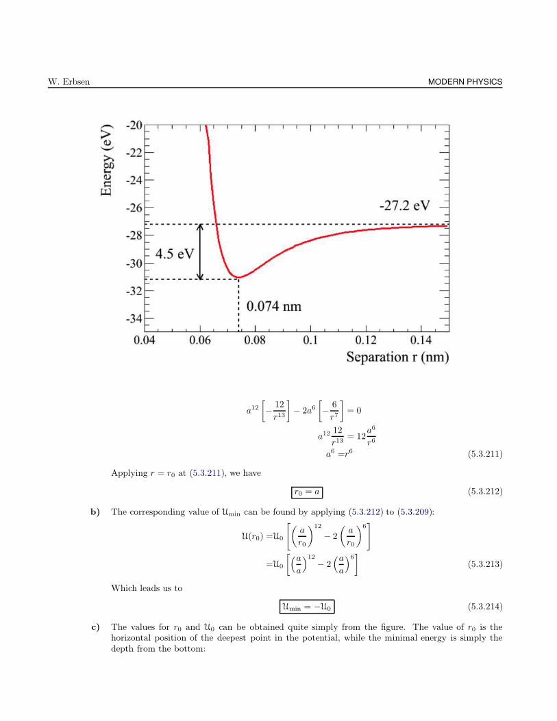
W. Erbsen MODERN PHYSICS
a12
[− 12
r13
]− 2a6
[− 6
r7
]= 0
a12 12
r13= 12
a6
r6
a6 =r6 (5.3.211)
Applying r = r0 at (5.3.211), we have
r0 = a (5.3.212)
b) The corresponding value of Umin can be found by applying (5.3.212) to (5.3.209):
U(r0) =U0
[(a
r0
)12
− 2
(a
r0
)6]
=U0
[(aa
)12
− 2(aa
)6]
(5.3.213)
Which leads us to
Umin = −U0 (5.3.214)
c) The values for r0 and U0 can be obtained quite simply from the figure. The value of r0 is thehorizontal position of the deepest point in the potential, while the minimal energy is simply thedepth from the bottom:
CHAPTER 5: DEPARTMENTAL EXAMINATIONS 493
r0 = 0.074 nm
Umin = −|27.2 eV − 4.5eV| −→ Umin = −31.7 eV
Problem 28
The measured conductivity of copper at room temperature is 5.88 × 10⁷ Ω−1 · m−1, its Fermi energy is 7.03eV,density is 8.96g m/cm3 and molar mass is 63.5gm/mole.
a) Calculate the density of free electrons in copper.
b) Calculate the average time between collisions of the conduction electrons.
c) Calculate the mean free path of electrons in copper.
d) Calculate the smallest possible deBroglie wavelength of electrons in copper at T = 0K. How does this valuecompare with the atomic separation in copper?
Solution
a) Copper has only one free (valence) electron. According to the Free Electron Approximation, all theconductivity is due to this one electron per copper atom. So, if we wanted to calculate the density
of free electrons in copper, we recall that ρ = M/V , and since we have only one free electron peratom, we find the density as
n =(ρCu
m
)·NA
=8.96g
cm3·(63.5 · g
mol
)−1
· 6.022× 1023 atoms
mol
=8.96g
cm3·(
1
63.5· mol
g
)· 6.022× 10²³ atoms
mol(5.3.215)
From (5.3.215), it is easy to see that we are left simply with
n = 8.497× 10²² atoms
cm3(5.3.216)
b) In order to calculate the average time between collisions of the conduction electrons, we first mustconsider the kinetic energy of these electrons, and from that find the average velocity:
E =mv2
2−→ v =
√2E
m(5.3.217)
Where we take E in (5.3.217) to be the Fermi Energy, EF , which is given in the prompt. Accordingly,we can evaluate v in (5.3.217) as
v =
√2 (7.03 eV)
(0.511× 10⁶ eV)· (3 × 10⁸ m/s)
2 −→ v = 1.574× 10⁶ m
s(5.3.218)
W. Erbsen MODERN PHYSICS
We now recall that the conductivity is defined as
σ =ne2d
mv(5.3.219)
Where we recognize that the relationship between velocity, the time between collisions and thedistance traveled between collisions is v = d/τ → d/v = τ . Substituting this into (5.3.219),
σ =ne2
m·(
d
v
)
=ne2
m· τ (5.3.220)
Solving (5.3.220) for τ yeilds
τ =mσ
ne2
=
(9.109× 10⁻³¹ Kg
) (5.880× 10⁷ Ω−1 · m−1
)
(8.497× 10²² atoms · cm−3) (100 cm ·m−1)3(1.602× 10⁻¹⁹ C)
2 (5.3.221)
Evaluating all the goodness in (5.3.221) leaves us with
τ = 2.462× 10⁻¹⁴ s (5.3.222)
c) The mean free path is found from the velocity found in part b) as
d =v · τ=(1.574× 10⁶ m · s−1
) (2.462× 10⁻¹⁴ s
)−→ d = 38.75 nm (5.3.223)
d) The deBroglie wavelength can be found rather straightforwardly using (5.3.218) as
λ =h
p=
6.626× 10⁻³⁴ J · s(9.109× 10⁻³¹ Kg) (1.574× 10⁶ m · s−1)
(5.3.224)
From (5.3.224) we see that
λ = 4.621× 10⁻¹⁰ m (5.3.225)
The atomic separation of copper can be found from the density, ρ, which is given in the problem:
ρ =m
v=m
L3−→ L =
[m
ρ
]1/3
(5.3.226)
Substituting in the appropriate values into (5.3.226) yields
L =
[(63.5 g · mol−1
) (6.022× 10²² atoms ·mol−1
)
(8.96 g · cm3) (100 cm · m−1)3
]−→ L = 2.275× 10⁻¹⁰ m
Problem 29
The proper mean lifetime of π Mesons (Pions) is 2.6× 10⁻⁸ s. If a beam of such particles has a speed of 0.9 c:
CHAPTER 5: DEPARTMENTAL EXAMINATIONS 495
a) What would their mean life be as measured in the laboratory?
b) How far would they travel (on the average) before they decay?
c) What would your answer be to part b) if you neglect time dilation?
d) What is the interval in space-time between creation of a typical pion and its decay?
Solution
We first recall that the equation for time-dilation is
T = γT0 (5.3.227)
Where the Lorentz factor, γ, is equal to
γ =1√
1 − v2/c2(5.3.228)
a) In the lab frame, using (5.3.227)-(5.3.228) we have
T =2.6× 10⁻⁸ s√
1 − (0.9)2−→ T = 5.965× 10⁻⁸ s (5.3.229)
b) In the lab frame, we know that ∆x = v · T , and using (5.3.229), we have
∆x = (0.9)(3 × 10⁸ m · s−1
) (5.965× 10⁻⁸ s
)−→ ∆x = 16.105 m (5.3.230)
c) If time-dilation is neglected, we can find ∆x as
∆x = (0.9)(3 × 10⁸ m · s−1
) (2.6× 10⁻⁸ s
)−→ ∆x = 7.020 m
d) The Space-time interval is defined as
∆s2 = −∆x2 + c2∆T 2 (5.3.231)
Substituting in the appropriate values into (5.3.231),
∆s2 =(3 × 10⁸ m · s−1
) (5.965× 10⁻⁸ s
)2 − (16.105 m)2 −→ ∆s2 = 60.86 m2
So, the space-time interval is
∆s =√
60.86 m2 −→ ∆s = 7.801 m
Problem 30
Four identical, non-interacting particles are placed in a one dimensional box of length L. Find the lowest to-tal energy of the system and list the quantum numbers of all occupied states (including ms) if:
a) The particles are electrons
W. Erbsen MODERN PHYSICS
b) The particles are neutral Pions, π0.
c) Two of the particles are protons and the other two are neutrons.
Solution
We first recall that the 1-D, time independent SE reads
− ~2
2m
∂2
∂x2ψ(x) = Eψ(x) (5.3.232)
Solving (5.3.232) with the appropriate boundary conditions, we find that the corresponding Eigenfunctionand Eigenvalues are, respectively
ψ(x) =
√2
Lsin(nπxL
)(5.3.233a)
En =n2~2π2
2mL2(5.3.233b)
a) Since electrons are Fermions, no two electrons can be described by the same set of quantum numbers,as necessitated by the Pauli Exclusion Principle. Therefore, the lowest occupied states are:
|n,ms〉 = |1, 1/2〉, |1, −1/2〉, |2, 1/2〉, |2, −1/2〉
And from (5.3.233b), the lowest energy corresponding to this state is
Egs =~2π2
2mL2[1 + 1 + 4 + 4] −→ Egs =
5~2π2
meL2
b) The neutral pion has a spin of zero, making it a Boson. Since the Pauli Exclusion principle doesnot apply to Bosons, all the particles may lie in the lowest state:
|n,ms〉 = |1, 0〉, |1, 0〉, |1, 0〉, |1, 0〉
While the energy is, following (5.3.233b),
Egs =~2π2
2mL2[1 + 1 + 1 + 1] −→ Egs =
2~2π2
mπL2
c) Both Protons and Neutrons are Fermions, but they are distinguishable from one another. Therefore,the lowest state is then
|n,ms〉 = |1, 1/2〉, |1, −1/2〉, |1, 1/2〉, |1, −1/2〉
And the Eigenenergies are
Egs =~2π2
2mpL2[1 + 1] +
~2π2
2mnL2[1 + 1] −→ Egs =
~2π2
L2
(1
mp+
1
mn
)
CHAPTER 5: DEPARTMENTAL EXAMINATIONS 497
5.4 Statistical Mechanics
Problem 1
a) Define the chemical potential µ. Show that two systems are in diffusive equilibrium if µ1 = µ2. You maystart with F = F1 + F2 (free energy) and use the fact that µ1 = µ2 should minimize F .
b) Now consider a 1−D gas of length L and number of distinguishable and non-interacting particles N . Assumethat temperature T is high enough that we are in the classical regime. Find the chemical potential µ in termsof T and other parameters of the problem.
c) Now find the free energy F and the specific heat at constant volume CV .
Solution
a) The chemical potential, µ, can be thought of as a number that allows us to quantify whether or nottwo (or more) systems are in diffusive equilibrium.
If they are equal, then there will be no (net) flux of particles moving from one system to another.If they are not equal, then particles will tend to flow from a region of high chemical potential to aregion of low chemical potential.
We also recall that the Helmholtz Free Energy (F ) measures the amount of “useful” work thatis extractable from a system at constant temperature and volume. The Free Energy has severalimportant characteristics:
i) At equilibrium, the Free Energy is at a minimum
ii) An important form of the second law of thermodynamics is
U = F + TS
Where U is the internal energy, and S is the final entropy.
At diffusive equilibrium, we know that dF = 0, and the number of particles in each system remainsconstant. From this, we may also deduce that the total number of particles remains constant.Quantitatively,
N = N1 +N2
In fact, whether we are in diffusive equilibrium or not, the total number of particles must remainconstant! That is,
0 = dN1 + dN2 −→ dN1 = −dN2 (5.4.1)
We can also think of the free energy of each system, as we did with the particle number previously.The total free energy would be described by
F = F1 + F2 (5.4.2)
And when we are in diffusive equilibrium, according to our first stipulation, F must be minimizedwith respect to the particle number:
W. Erbsen STATISTICAL MECHANICS
dF
dN= 0 (5.4.3)
Combining (5.4.1) and (5.4.2),
dF =∂F1
∂N1dN1 +
∂F2
∂N2dN2 (5.4.4)
Setting (5.4.4) equal to zero, as demonstrated in (5.4.3), we have
∂F1
∂N1dN1 = − ∂F2
∂N2dN2 (5.4.5)
Applying (5.4.1) once again to (5.4.5), we are left with
∂F1
∂N1dN1 = − ∂F2
∂N2(−dN1) −→
∂F1
∂N1=∂F2
∂N2(5.4.6)
We now recall that the chemical potential is defined by
µ =
(∂F
∂N
)
V,T
(5.4.7)
Applying the definition of chemical potential from (5.4.7) to our result (5.4.6), it is easy to see thatat equilibrium,
µ1 = µ2
b) We are tasked with finding the chemical potential for distinguishable, non-interacting particles inthe classical regime for a 1-D gas. As we do in all of statistical mechanics, we begin by finding the(single particle) partition function:
Z1 =∑
i
exp
[− Ei
kBT
](5.4.8)
For a classical gas, the energy will come in the form of the kinetic energy, which is E = p2/(2m).Furthermore, within the classical regime, we may take our energy distribution to be continuous,and as such may be integrated in the following way:
Z1 =1
h3
∫exp
[− p2
2mkBT
]d3p
∫d3x (5.4.9)
For a 1-D gas, as is the case here, (5.4.9) becomes
Z1 =1
h
∫ ∞
−∞exp
[− p2
2mkBT
]dp
∫ L
0
dx
=1
h·[√
2πmkBT]· [L]
=L
h
√2πmkBT (5.4.10)
Within the classical approximation, the full partition function can be approximated by
ZN∼= ZN
1
Applying this to the single particle partition function of (5.4.10), we have
CHAPTER 5: DEPARTMENTAL EXAMINATIONS 499
ZN =
[L
h
√2πmkBT
]N
(5.4.11)
We now recall that the Free energy takes the form
F = −kBT log [ZN ] (5.4.12)
Substituting (5.4.11) into (5.4.12),
F = − kBT log
[L
h
√2πmkBT
]N
= −NkBT log
[L
h
√2πmkBT
](5.4.13)
Now, we recall that the chemical potential, given by (5.4.7), can be calculated from (5.4.13) as
µ =∂
∂N
[−NkBT log
[L
h
√2πmkBT
]](5.4.14)
The answer is then
µ = −kBT log
[L
h
√2πmkBT
]
c) From (5.4.13), F was found to be
F = −NkBT log
[L
h
√2πmkBT
]
To find the specific heat capacity at constant volume, we have to get back to work. Recall that thisquantity is defined as
CV =
(∂U
∂T
)
V
(5.4.15)
We also recall that the internal energy is given by
U = − ∂
∂βlog (ZN ) (5.4.16)
Now substituting (5.4.11) into (5.4.16),
U = − ∂
∂βlog
[L
h
√2πmkBT
]N
= −N∂
∂βlog
[L
h
√2πmkBT
]
= −N∂
∂βlog
[√2πmL2
βh2
]
= −N∂
∂βlog
[2πmL2
βh2
]1/2
W. Erbsen STATISTICAL MECHANICS
= − N
2
∂
∂βlog
[2πmL2
βh2
]
= − N
2
∂
∂βlog
[2πmL2
h2︸ ︷︷ ︸Garbage
1
β
](5.4.17)
The derivative of (5.4.17) comes out being very simple,
U =N
2· 1
β
=NkBT
2(5.4.18)
Putting our cleaned up expression back into (5.4.15), we find CV :
CV =∂
∂T
[NkBT
2
]−→ CV =
NkB
2
Problem 2
Consider a particle in a 1-dimensional box of side L with available energy levels (in the presence of a magneticfield B along z)
εn = γ2n2 + m · B; γ2 =~2
2m
(πL
)2
(5.4.19)
Where n is an integer greater than zero and m = ±mz k.
a) What is the partition function for this particle?
b) What is the partition function for N classical, identical, noninteracting particles in the same box in thepresence of a magnetic field? Hence find an expression for the internal energy U , and the Helmholtz freeenergy F .
c) What is the equilibrium pressure and magnetization of this gas?
Solution
From the information supplied,
En = γ2n2 + m · B
γ2 =~2
2m
(πL
)2
→ En =n2~2π2
2mL2+ m · B (5.4.20)
a) The first step in this problem, as is in most problems in this field, is to find the partition function.Let’s ride this pony:
Z1 =∑
n
exp
[− En
kBT
]=∑
n
exp [−Enβ] (5.4.21)
CHAPTER 5: DEPARTMENTAL EXAMINATIONS 501
Substituting (5.4.20) into (5.4.21),
Z1 =∑
n
exp
[−[n2~2π2
2mL2+ m · B
]β
]
=∑
n
exp
[−n
2~2π2
2mL2β −m · Bβ
]
=∑
n
exp
[−n
2~2π2
2mL2β −±mzB0β
](5.4.22)
I changed m ·B → ±mzB0. Because of the ± in front of the spin quantum number, we need to split(5.4.22) into two distinct sums, each addressing its respective parity. With this, (5.4.22) is now
Z1 =∑
n
exp
[−n
2~2π2
2mL2β −mzB0β
]+ exp
[−n
2~2π2
2mL2β +mzB0β
](5.4.23)
At this point, we turn to our calculus loving friends and with a tote on their pipe I decide to go theway of the integral. And it was so, the sum was transferred into an integral, and (5.4.23) becomes
Z1 =
∫ ∞
0
exp
[−n
2~2π2
2mL2β −mzB0β
]+ exp
[−n
2~2π2
2mL2β +mzB0β
]dn
=
∫ ∞
0
exp
[−n
2~2π2
2mL2β
]exp [−mzB0β] + exp
[−n
2~2π2
2mL2β
]exp [mzB0β]
dn
=exp [−mzB0β]
∫ ∞
0
exp
[−n
2~2π2
2mL2β
]dn + exp [mzB0β]
∫ ∞
0
exp
[−n
2~2π2
2mL2β
]dn
=exp [−mzB0β]
∫ ∞
0
exp
[−β~2π2
2mL2n2
]dn+ exp [mzB0β]
∫ ∞
0
exp
[−β~2π2
2mL2n2
]dn
= exp [−mzB0β] + exp [mzB0β]∫ ∞
0
exp
[−β~2π2
2mL2n2
]dn
=2 cosh [mzB0β]
∫ ∞
0
exp
[−β~2π2
2mL2n2
]dn
=2 cosh [mzB0β]
[1
2
√2πmL2
β~2
](5.4.24)
From (5.4.24), it is easy to see that the partition function becomes
Z1 = cosh [mzB0β]
√2πmL2
β~2(5.4.25)
b) But what if the partition function is to be applied to a classical, indistinguishable, non-interactingsystem? From this we must find the internal energy U , as well as the free energy F .
We first recall that since we have indistinguishable particles, the full partition function can befound from the single-particle partition function as
ZN∼= ZN
1
N !(5.4.26)
Rearranging the single particle partition function (5.4.25) and applying (5.4.26), we have
W. Erbsen STATISTICAL MECHANICS
ZN =1
N !
[cosh [mzB0β]
√2πmL2
β~2
]N
(5.4.27)
Now, the free energy is
F = −kBT log [ZN ] (5.4.28)
And plugging (5.4.27) into (5.4.28),
F = −kBT
log
[cosh [mzB0β]
√2πmL2
β~2
]N− log [N !]
(5.4.29)
At this point, we recall Stirling’s Approximation:
log [N !] ∼= N log [N ]−N
Applying this to (5.4.29),
F = − kBT
log
[cosh [mzB0β]
√2πmL2
β~2
]N− (N log [N ] −N)
= − kBT
N log
[cosh [mzB0β]
√2πmL2
β~2
]−N log [N ] +N
= −NkBT
log
[cosh [mzB0β]
√2πmL2
β~2
]− log [N ] + 1
(5.4.30)
Simplifying (5.4.30) further leads us to
F = −NkBT
log
[cosh [mzB0β]
N
√2πmL2
β~2
]+ 1
(5.4.31)
To find the internal energy, U , we first recall that
U = − ∂
∂βlog [ZN ] (5.4.32)
Substituting the partition function from (5.4.27) into (5.4.32),
U = − ∂
∂βlog
1
N !
[cosh [mzB0β]
√2πmL2
β~2
]N
= −N∂
∂βlog
[1
N !1/N
[cosh [mzB0β]
√2πmL2
β~2
]]
= −N∂
∂βlog
[1
N !1/N
√2πmL2
~2︸ ︷︷ ︸
Garbage
cosh [mzB0β]√β
]
Proceeding,
CHAPTER 5: DEPARTMENTAL EXAMINATIONS 503
U = −N∂
∂βlog
[cosh [mzB0β]√
β
]
= −N∂
∂β
log [cosh [mzB0β]] − log
[√β]
= −N
∂
∂βlog [cosh [mzB0β]] − 1
2
∂
∂βlog [β]
(5.4.33)
Playing around with (5.4.33) a bit we can see that we have our answer:
U = −NmzB0 tanh [mzB0β] − 1
2β
(5.4.34)
c) In order to find the equilibrium pressure, we first recall that
P = −∂F∂V
⇒ −∂F∂L
(5.4.35)
Where I took V → L since we are only in 1-D. Anyway, we can substitute our value for the FreeEnergy from (5.4.31) into (5.4.35):
P = − ∂
∂L
[−NkBT
log
[cosh [mzB0β]
N
√2πmL2
β~2
]+ 1
]
=NkBT∂
∂L
[log
[cosh [mzB0β]
N
√2πmL2
β~2
]+ 1
]
=NkBT∂
∂L
[log
[L
cosh [mzB0β]
N
√2πm
β~2
]+ 1
︸ ︷︷ ︸Garbage
](5.4.36)
Eww smelly garbage yuck yuck. Anyway, ignoring the icky garbage, (5.4.36) becomes
P =NkBT∂
∂L[L] −→ P =
NkBT
L(5.4.37)
The Magnetization, however, is a different story entirely. The relationship we are interested in is
M = −∂F∂B
(5.4.38)
Substituting our previous value of F into (5.4.38) yields
M = − ∂
∂B
[−NkBT
log
[cosh [mzB0β]
N
√2πmL2
β~2+ 1
]]
=NkBT∂
∂Blog
[cosh [mzB0β]
N
√2πmL2
β~2+ 1
]
=NkBT∂
∂Blog
[cosh [mzB0β]
1
N
√2πmL2
β~2+ 1
]
M =NkBT∂
∂Blog
[cosh [mzB0β]
]
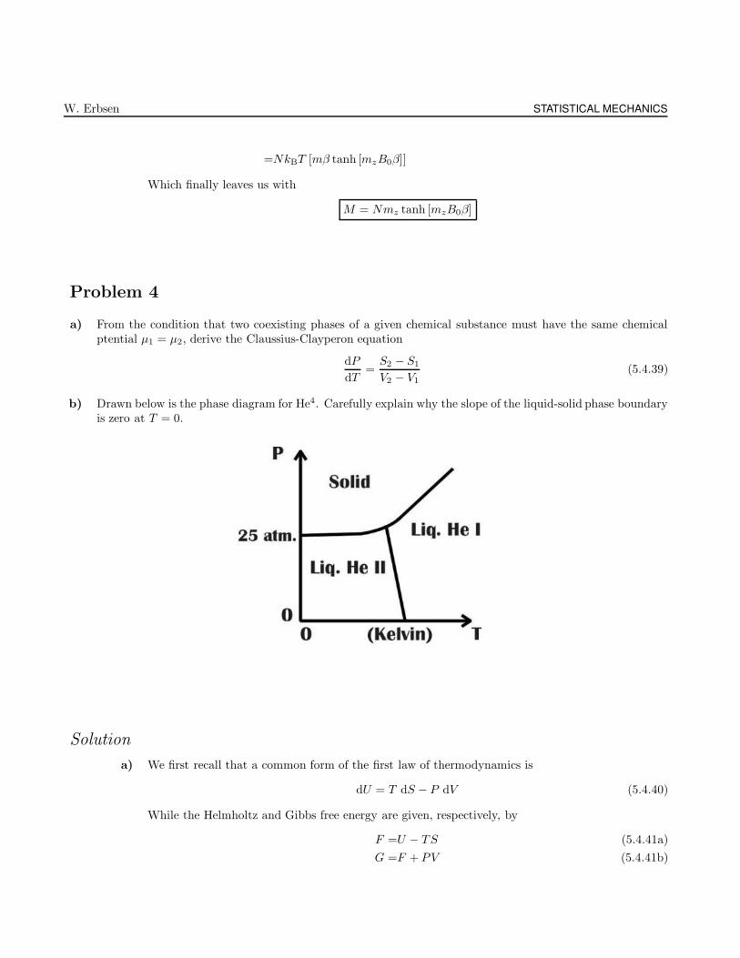
W. Erbsen STATISTICAL MECHANICS
=NkBT [mβ tanh [mzB0β]]
Which finally leaves us with
M = Nmz tanh [mzB0β]
Problem 4
a) From the condition that two coexisting phases of a given chemical substance must have the same chemicalptential µ1 = µ2, derive the Claussius-Clayperon equation
dP
dT=S2 − S1
V2 − V1(5.4.39)
b) Drawn below is the phase diagram for He4. Carefully explain why the slope of the liquid-solid phase boundaryis zero at T = 0.
Solution
a) We first recall that a common form of the first law of thermodynamics is
dU = T dS − P dV (5.4.40)
While the Helmholtz and Gibbs free energy are given, respectively, by
F =U − TS (5.4.41a)
G =F + PV (5.4.41b)
CHAPTER 5: DEPARTMENTAL EXAMINATIONS 505
If we make the substitution (5.4.41a) into (5.4.41b), we have
G = U − TS + PV (5.4.42)
Taking (5.4.42) to the differential limit, we have
dG =dU − T dS − S dT + P dV + V dP
=dU − (T dS − P dV ) − s dT + V dP
=dU − dU − S dT + V dP
= − S dT + V dP (5.4.43)
Where I substituted in (5.4.40) in the second to last step arriving at (5.4.43). We now recall thatthe chemical potential is given by
µ =
(∂F
∂N
)
V,T
⇒ ∂G
∂N(5.4.44)
We can now play around with (5.4.44) as follows
µ =∂G
∂N−→ dµ =
G
N−→ dG = Ndµ (5.4.45)
Applying (5.4.45) to (5.4.43),
n dµ =V dP − S dT
dµ =V
NdP − S
NdT (5.4.46)
We now temporarily recall that since we are at diffusive equilibrium, then µ1 = µ2 and furthermore,dµ1 = dµ2. Ergo, (5.4.46) is transformed into
V1
NdP − S1
NdT =
V2
NdP − S2
NdT
V1
NdP − V2
NdP =
S1
NdT − S2
NdT
dP (V1 − V2) =dT (S1 − S2) (5.4.47)
From (5.4.47), it is most easily seen that
dP
dT=S1 − S2
V1 − V2(5.4.48)
b) We are given a phase diagram for He4, which we immediately recognize as a Boson. This is especiallyinteresting because Bosons do not obey the Pauli Exclusion Principle, and can therefore all occupythe same state at an arbitrarily low temperature. The multiplicity, that is, the number of statesavailable to a system without changing anything, is only 1. e.g., at low temperatures, there is only1 way that the system can be configured (all in the ground state), and subsequently the multiplicityis Ω = 1.
This is particularly interesting, since He4 has a multiplicity of 1, then the entropy is 0:
S = kBT log [Ω] −→ S = kBT log [1] −→ S = 0
The Claussius-Clayperon equation that we derived earlier in (5.4.48) describes the slope of the phaseboundaries. In the case that we have low temperatures (approaching zero), where the multiplicity,
W. Erbsen STATISTICAL MECHANICS
Ω, is 1, while the entropy, S, is 0. Plugging this in to (5.4.48), we get
dP
dT=
0 − 0
V1 − V2−→ dP
dT= 0
The Claussius-Clayperon equation can be thought of as the “slope equation” for phase diagrams.When the result is zero, that implies that there is no slope, and so you get a straight line.
Problem 5
Consider an ideal gas of diatomic molecules. The rotational motion is quantized according to εj = j(j + 1)ε0, j =0, 1, 2, ... The multiplicity of each rotational level is gj = 2j + 1.
a) Find the rotational part of the partition function Z for one molecule.
b) Convert the sum (for Z) to an integral and evaluate the integral for kT ε0. From this find an expressionfor the specific heat capacity at constant volume at low temperatures.
Solution
a) For a system consisting of degeneracy, the form of the partition function that we will employ is
Z1 =∑
j
gj exp
[− Ej
kBT
](5.4.49)
In our case, we have
gj = 2j + 1 , εj = j(j + 1) ε0
Applying both of these to our single-particle partition function in (5.4.49), we have
Z1 =∑
j
(2j + 1) exp
[−j(j + 1) ε0
kBT
](5.4.50)
b) Converting the sum in (5.4.50) into an integral:
Z1 =
∫ ∞
0
(2j + 1) exp
[−j(j + 1) ε0
kBT
]dj (5.4.51)
u = j(j + 1) = j2 + jdu = 2j + 1 dj
And using this du substitution, we can transform (5.4.51) into
Z1 =
∫ ∞
0
exp
[− uε0kBT
]du
= − kBT
ε0
[exp
[− uε0kBT
]∣∣∣∣∞
0
CHAPTER 5: DEPARTMENTAL EXAMINATIONS 507
From which it is easy to deduce that
Z1 =kBT
ε0(5.4.52)
We need to move away from the single-particle partition function, and since we are dealing indis-tinguishable entities:
ZN∼= ZN
1
N !(5.4.53)
Substituting the single particle partition function from (5.4.52) into (5.4.53),
ZN =1
N !
(kBT
ε0
)N
(5.4.54)
Now hold on to yer britches, and recall that
CV =
(∂U
∂T
)
V
, U = − ∂
∂βlog [ZN ]
First, let’s evaluate the internal energy U , by substituting into (5.4.54) this expression:
U = − ∂
∂βlog
[1
N !
(1
βε0
)N]
= −N∂
∂βlog
[1
N ! 1/N
(1
βε0
)]
= −N∂
∂βlog
[1
N !1/N
(1
ε0
)
︸ ︷︷ ︸
1
β
](5.4.55)
And (5.4.55) becomes
U = −N∂
∂βlog
[1
β
](5.4.56)
Carrying out the simple derivative in (5.4.56) leads us to
U =N
β−→ u = NkBT (5.4.57)
To find the specific heat, we substitute the internal energy (5.4.57) into the appropriate formula
CV =∂
∂T(nkBT ) −→ CV = NkB
For an ideal gas with three degrees of freedom, we find that
U =3
2NkBT
And so the specific heat at constant volume becomes
CV =5
2NkB
W. Erbsen STATISTICAL MECHANICS
Problem 6
a) Write down the Grand Partition Function (Gibbs sum), Ω. Define all quantities used and explain what thesummations are over.
b) Show that the average number of particles in a Grand Canonical Ensemble is given by
〈N〉 = τ∂
∂µlog Ω (5.4.58)
where τ = kT and µ is the chemical potential.
c) Now consider a dilute gas of hydrogen atoms. Assume each atom may have the following states:
State No. of Electrons Energy
Ground 1 0Positive ion 0 −∆Negative ion 2 +δ
Find the condition that the average number of electrons per atom is 1.
Solution
a) We recall that within the framework of the Grand Canonical Ensemble, the system in question isin both thermal and diffusive equilibrium. The sum itself takes the form
Ω (µ, T ) =
∞∑
N=0
∑
s(N)
exp
[Nµ− Es,N
kBT
](5.4.59)
Ω = The Gibbs Sumµ = The Chemical PotentialN = The Number of Particles
Es,N = The energy of N-particles in S-states
b) We recall that, in general, the average number of particles is
〈N〉 =∑
s,N
N · P (N,Es,N) (5.4.60)
Where the probability function is given by
P (N,Es,N) =1
Ω (µ, T )· exp
[Nµ −Es,N
kBT
](5.4.61)
And substituting the probability function (5.4.61) back into (5.4.60) to find the average number ofparticles,
〈N〉 =∑
s,N
N · 1
Ω (µ, T )· exp
[NU − Es,N
kBT
](5.4.62)
For the time being, let’s take the following (seemingly) arbitrary derivative:
CHAPTER 5: DEPARTMENTAL EXAMINATIONS 509
∂Ω (µ, T )
∂µ=∂
∂µ
∑
N,s(N)
exp
[Nµ −Es,N
kBT
]
=∑
N,s(N)
N
kBTexp
[Nµ− Es,N
kBT
]
=1
kBT
∑
N,s(N)
N exp
[Nµ− Es,N
kBT
](5.4.63)
Solving (5.4.63) for the portion that resembles a part of (5.4.62),
kBT · ∂
∂µΩ (µ, T ) =
∑
N,s(N)
N exp
[Nµ− Es,N
kBT
](5.4.64)
We can substitute the RHS of (5.4.64) into (5.4.62):
〈N〉 =∑
s,N
kBT
Ω (µ, T )· ∂∂µ
Ω (µ, T ) (5.4.65)
Let’s rewrite (5.4.65):
〈N〉 =∑
s,N
kBT1
Ω (µ, T )· ∂∂µ
Ω (µ, T )
︸ ︷︷ ︸(5.4.66)
Let’s look a little closer at the Gibbs function from (5.4.59) (ignore sums momentarily):
Ω (µ, T ) = exp
[Nµ−Es,N
kBT
]
Let’s take the first derivative with respect to µ:
∂
∂µΩ (µ, T ) =
∂
∂µexp
[Nµ− Es,N
kBT
]
=N
kBTexp
[Nµ−Es,N
kBT
](5.4.67)
If we take the first derivative of the Gibbs function with respect to µ, we get some coefficient times
the original function. Now, there’s two ways of getting rid of the original function: assuming thatyou just want to play around with the coefficients for some reason. You could a) simply divide youranswer by the original function, or b), you could take the same derivative you took before, but hadthe natural log of the function:
1
Ω (µ, T )· ∂∂µ
Ω (µ, T ) =∂
∂µlog [Ω (µ, T )] (5.4.68)
We note that the LHS of (5.4.68) is identical to the underbraced term in (5.4.66). Substituting theRHS of (5.4.68) into (5.4.66), replacing the underbraced term, we have:
〈N〉 =∑
s,N
kBT∂
∂µlog [Ω (µ, T )] (5.4.69)
Rearranging, (5.4.69) becomes
W. Erbsen STATISTICAL MECHANICS
〈N〉 = kBT∂
∂µlog [Ω (µ, T )] (5.4.70)
Where we note that the summation is implicit in the Gibbs function.
c) The first thing that we have to do is find the Gibbs sum. Using the probability function (5.4.61) asour outline, the sum itself takes the form
Ω (µ, T ) =
∞∑
N=0
∑
s(N)
exp
[Nµ−Es,N
kBT
](5.4.71)
There are only three unique states, so the second sum in (5.4.71) only goes to 3. We also know thatwe have three states of electrons, of occupancy 0, 1, or 2 as given in the provided table. Accordingly,(5.4.71) becomes
Ω (µ, T ) = exp
[(1)µ− 0
kBT
]+ exp
[(0)µ − (−∆)
kBT
]+ exp
[(2)µ− (δ)
kBT
]
=exp
[µ
kBT
]+ exp
[∆
kBT
]+ exp
[2µ− δ
kBT
]
=exp [µβ] + exp [∆β] + exp [(2µ− δ) β] (5.4.72)
Substituting (5.4.72) into the equation for average number of particles from (5.4.70),
〈N〉 =1
β
∂
∂µlog [exp [µβ] + exp [∆β] + exp [(2µ− δ)β]]
=1
β
[β exp [µβ] + 2β exp [(2µ− δ)β]
exp [µβ] + exp [∆β] + exp [(2µ− δ)β]
]
=exp [µβ] + 2 exp [(2µ− δ)β]
exp [µβ] + exp [∆β] + exp [(2µ− δ)β](5.4.73)
We are actually looking for a condition where 〈N〉 = 1, so setting this in (5.4.73) yields
exp [µβ] + exp [∆β] + exp [(2µ− δ)β] = exp [µβ] + 2 exp [(2µ− δ)β]
exp [∆β] = exp [(2µ− δ)β]
∆β = (2µ− δ)β (5.4.74)
From (5.4.74), one of the conditions that might be met is in terms of the chemical potential, whichreads
µ =∆ + δ
2
Problem 7
A system of N distinguishable noninteracting particles has one-particle energy levels of En = nε, where thedegeneracy of the nth level is equal to n, and n = 1, 2, 3, ...
CHAPTER 5: DEPARTMENTAL EXAMINATIONS 511
a) Show that the partition function of the system is
Z =
[eβε
(eβε − 1)2
]N
(5.4.75)
where β = (kBT )−1
.
b) Calculate the entropy of the system of particles.
c) Determine the behavior of the entropy at high temperature.
d) Determine the behavior of the specific heat at high temperatures.
Solution
We first recognize that since we have distinguishable particles, then the partition function as a functionof the single-particle partition function would be ZN
∼= ZN1 .
a) The standard form of the partition function (with degeneracy) is
Z1 =∑
n
n · exp
[− En
kBT
](5.4.76)
We now substitute En = nε into (5.4.76),
Z1 =∑
n
n · exp
[− nε
kBT
](5.4.77)
We can rewrite (5.4.77) slightly,
Z1 =∑
n
n · exp
[− ε
kBT
]n
(5.4.78)
And now, we see that if we were to take some arbitrary derivative of some function then the answercould be (5.4.78). One such form is
Z1 = −1
ε
∂
∂β
∑
n
n · exp [−εβ]n
(5.4.79)
Where I have changed form kBT to β−1. We now recall the following summation identity:∑
rn =r
1 − r
Applying this to (5.4.79),
Z1 = − 1
ε
∂
∂β
[exp [−εβ]
1 − exp [−εβ]
]
= − 1
ε
∂
∂β
[exp [−εβ]
1 − exp [−εβ]
]
= − 1
ε
exp [−εβ]
[∂
∂β
1
1 − exp [−εβ]
]+
1
1 − exp [−εβ]
[∂
∂βexp [−εβ]
]
W. Erbsen STATISTICAL MECHANICS
= − 1
ε
exp [−εβ]
[−ε exp [−εβ]
(1 − exp [−εβ])2
]+
1
1 − exp [−εβ][−ε exp [−εβ]]
=exp [−2εβ]
(1 − exp [−εβ])2 +
exp [−εβ]
1 − exp [−εβ]
=exp [−2εβ]
(1 − exp [−εβ])2+
exp [−εβ]
1 − exp [−εβ]· 1 − exp [−εβ]
1 − exp [−εβ]
=exp [−2εβ] + exp [−εβ] − exp [−2εβ]
(1 − exp [−εβ])2
=exp [−εβ]
(1 − exp [−εβ])2
=exp [−εβ]
1 − 2 exp [−εβ] + exp [−2εβ]· exp [2εβ]]
exp [2εβ]]
=exp [εβ]
exp [2εβ] − 2 exp [εβ] + 1(5.4.80)
We an finally say that (5.4.80) can be reduced to
Z1 =exp [εβ]
(exp[εβ] − 1)2(5.4.81)
Converting (5.4.81) into the full partition function,
ZN =
[exp [εβ]
(exp[εβ] − 1)2
]N
(5.4.82)
b) To calculate the entropy for a system of particles, we first recall that
S = −∂F∂T
(5.4.83)
So, we first need to find F :
F = −kBT log [ZN ] (5.4.84)
Substituting the partition function (5.4.82) into (5.4.84),
F = − kBT log
[exp [εβ]
(exp[εβ] − 1)2
]N
= −NkBT log
[exp [εβ]
(exp[εβ] − 1)2
]
= −NkBT
log [exp [εβ]] − log[(exp [εβ] − 1)
2]
= −NkBT log [exp [εβ]]− 2 log [(exp [εβ] − 1)] (5.4.85)
Substituting (5.4.85) back into (5.4.83), we can find S,
S = − ∂
∂T[−NkBT log [exp [εβ]]− 2 log [(exp [εβ] − 1)]]
CHAPTER 5: DEPARTMENTAL EXAMINATIONS 513
=NkB∂
∂T
[T log
[exp
[ε
kBT
]]+ 2 log
[(exp
[ε
kBT
]− 1
)]]
=NkB∂
∂T
[ε
kB︸︷︷︸Garbage
+2 log
[exp
[ε
kBT
]−1︸︷︷︸
Don’t matter
]](5.4.86)
Rewriting (5.4.86):
S =2NkB∂
∂Tlog
[exp
[ε
kBT
]− 1
]
=2NkB
− ε
kBT
exp[
εkBT
]
exp[
εkBT
]− 1
(5.4.87)
Rearranging (5.4.87),
S = −2N
T
exp[
εkBT
]
exp[
εkBT
]− 1
(5.4.88)
Problem 8
In a mono-atomic crystalline solid each atom can occupy either a regular lattice site or an interstitial site. Theenergy of an atom at an interstitial site exceeds the energy of an atom at a lattice site by ε. Assume that thenumber of atoms, lattice sites, and interstitial sites are all equal in number.
a) Calculate the entropy of the crystal in the state where exactly n of the N atoms are at interstitial sites.
b) What is the temperature of the crystal in this state, if the crystal is at thermal equilibrium?
c) If ε = 0.5 eV and teh temperature of the crystal is 273 K, what is the fraction of atoms at interstitial sites?
Hint: You have two choices to make in this problem - which atoms to put at interstitial sites, and which interstitialsites to put them in.
Solution
a) To calculate the entropy, we recall that
S = −∂F∂T
(5.4.89)
And also that the Free energy is
F = −kBT log [ZN ] (5.4.90)
While the single-particle partition function in the case of degeneracy is
W. Erbsen STATISTICAL MECHANICS
Z1 =∑
i
gi · exp
[− Ei
kBT
](5.4.91)
Now, there are two different sources of degeneracy in this problem. There is one source comingfrom the n interstitial lattices, and then there is N for the regular lattices. So, combining theseinto (5.4.91), yields
Z1 =∑
n
n exp
[− En
kBT
]+∑
N
N exp
[− EN
kBT
](5.4.92)
Depending on where we are on the lattice we have a different energy, such that we should rewrite(5.4.92) as
Z1 =∑
n
n exp
[−(E0 + ε)
kBT
]+∑
N
N exp
[− E0
kBT
]
=exp
[− E0
kBT
]∑
n
n exp
[− ε
kBT
]+∑
N
N
(5.4.93)
At this point, we say that the degeneracy for this particular two-level case can be expressed in thefollowing more compact form:
g(N, n) =N !
(N − n)!n!(5.4.94)
Using this equation, we can completely transform (5.4.93), which now reads
ZN =N !
(N − n)!n!· exp
[− E0
kBT
]exp
[− ε
kBT
]+ 1
(5.4.95)
Using (5.4.90), we can now find the Free Energy by way of (5.4.95) as follows
F = − kBT log
N !
(N − n)!n!· exp
[− E0
kBT
]exp
[− ε
kBT
]+ 1
= − kBT
log
[N !
(N − n)!n!
]+ log
[exp
[− E0
kBT
]]+ log
[exp
[− ε
kBT
]+ 1
]
= − kBT
log
[N !
(N − n)!n!
]− E0
kBT+ log
[exp
[− ε
kBT
]+ 1
](5.4.96)
And to calculate the entropy, we now substitute (5.4.96) back in to (5.4.89):
S = − ∂
∂T
−kBT
log
[N !
(N − n)!n!
]− E0
kBT+ log
[exp
[− ε
kBT
]+ 1
]
=kB∂
∂T
T log
[N !
(N − n)!n!
]− E0
kB+ T log
[exp
[− ε
kBT
]+ 1
]
=kB
log
[N !
(N − n)!n!
]+ log
[exp
[− ε
kBT
]+ 1
]+ T
∂
∂Tlog
[exp
[− ε
kBT
]+ 1
]
=kB
log
[N !
(N − n)!n!
]+ log
[exp
[− ε
kBT
]+ 1
]+ T
[ε
T 2
exp [−ε/(kBT )]
exp [−ε/(kBT )] + 1
](5.4.97)
We can simplify (5.4.97) again:
CHAPTER 5: DEPARTMENTAL EXAMINATIONS 515
S = kB log
[N !
(N − n)!n!
]+ kB log
[exp
[− ε
kBT
]+ 1
]+ kB
ε
T
exp [−ε/(kBT )]
exp [−ε/(kBT )] + 1(5.4.98)
b) We recall that from the first law of thermodynamics,
dU = T dS − P dV (5.4.99)
At constant volume, (5.4.99) becomes
dU = T dS −→ dS
dU=
1
T(5.4.100)
Applying the chain rule to (5.4.100),
dS
dU=
dS
dU· dU
dn· dn
dU=
dS
dn· dn
dU=
1
T
And now,
U =n (E + ε) + (N − n)E
=nE + nε+NE − nE
=nε+NE
Taking the differential limit,
dU = ε dn −→ dn
dε=
1
ε
Substituting this back in to our chain rule,
dS
dn· 1
ε=
1
T−→ dS
dn=ε
T(5.4.101)
At this point, we apply (5.4.101) to (5.4.98):
dS
dn=
d
dn
kB log
[N !
(N − n)!n!
]+ kB log
[exp
[− ε
kBT
]+ 1
]+ kB
ε
T
exp [−ε/(kBT )]
exp [−ε/(kBT )] + 1
=kBd
dnlog
[N !
(N − n)!n!
](5.4.102)
We can further rewrite (5.4.102),
dS
dn=kB
d
dnlog [N !]− log [(N − n)!] + log [n!] (5.4.103)
Recall the identity
log [N !] = N log [N ]−N (5.4.104)
Using (5.4.104), we can rewrite (5.4.103) as:
dS
dn=kB
d
dnlog [(N − n)!] + n log [n] − n (5.4.105)
We can apply the same logic to the mixed term in (5.4.105):
log [(N − n)!] = (N − n) log [N − n] − (N − n)
W. Erbsen STATISTICAL MECHANICS
=N log [N − n] − n log [N − n] −N + n (5.4.106)
Substituting (5.4.106) back into (5.4.105),
dS
dn=kB
d
dnN log [N − n] − n log [N − n] −N + n+ n log [n] − n
=kBd
dnN log [N − n] − n log [N − n] + n log [n]
=kB
N
N − n− log [N − n]− n
N − n+ log [n] + 1
=kB
log
[N − n
n
]+
N
N − n− n
N − n+ 1
=kB
log
[N − n
n
]+ 2
(5.4.107)
We now set (5.4.107) to ε/T :
kB
log
[N − n
n
]+ 2
=ε
T(5.4.108)
Solving (5.4.108) for T ,
T =ε
kB
log
[N − n
n
]+ 2
−1
(5.4.109)
c) To find the fraction of atoms in the interstitial sites, we simply solve (5.4.109) for N/n:
ε
kBT= log
[N − n
n
]+ 2
exp
[ε
kBT− 1
]=N − n
n(5.4.110)
From (5.4.110) we can see that
N
n= exp
[ε
kBT− 1
]+ 1 (5.4.111)
Problem 9
Calculate the magnetic susceptibilityχ =
(∂M
∂H
∣∣∣∣H=0
(5.4.112)
Where M is the magnetic moment of the sample and H is the applied field. Calculate χ as a function of T of agas of N permanent dipoles, each of moment µ,
a) If any direction is allowed (classical spines).
b) If the dipole is only allowed to assume 2 directions, parallel and opposite to the applied field (Ising spins).
CHAPTER 5: DEPARTMENTAL EXAMINATIONS 517
Solution
a) The first thing that we recall is the energy of a dipole in an external field, which is given by
U = −µ · H (5.4.113)
And the magnetization is given by
M = − ∂F
∂H(5.4.114)
Now, if we have a whole bunch of dipoles, then they are not all perfectly aligned (or antialigned),but rather at some random angle θi. Then the total energy from the entirety of the molecules canbe found as
U = − µ · H∑
i
cos θi
= − µH∑
i
cos θi (5.4.115)
Since the particles in this case are distinguishable, the full partition function can be found from thesingle particle partition function as ZN
∼= ZN1 . The single-particle partition function is
Z1 =∑
i
exp
[µH cos θi
kBT
](5.4.116)
Turning the sum in (5.4.116) into an integral, we have
Z1 =
∫ 2π
0
∫ π
0
exp
[µH cos θ
kBT
]sin θ dθdφ (5.4.117)
Letting u = cos θ and du = − sin θ dθ, (5.4.117) becomes
Z1 = − 2π
∫ −1
1
exp
[µHu
kBT
]du
= − 2π · kBT
µH
[exp
[µHu
kBT
]∣∣∣∣−1
1
= − 2π · kBT
µH
exp
[−µHkBT
]− exp
[µH
kBT
]
=4π · kBT
µHsinh
[−µHkBT
](5.4.118)
The full partition function can be found from (5.4.118) easily as
ZN =
[4π · kBT
µHsinh
[−µHkBT
]]N
(5.4.119)
We now use (5.4.119) to find the Free Energy, F :
F = − kBT log [ZN ]
= − kBT log
[−4π · kBT
µHsinh
[µH
kBT
]]N
W. Erbsen STATISTICAL MECHANICS
= −NkBT log
[−4π · kBT
µHsinh
[µH
kBT
]](5.4.120)
We now substitute F from (5.4.120) into (5.4.114), the equation for the Magnetization, M :
M = − ∂
∂H
−NkBT log
[−4π · kBT
µHsinh
[µH
kBT
]]
=NkBT∂
∂Hlog
[−4π · kBT
µHsinh
[µH
kBT
]]
=NkBT∂
∂H
log
[4πkBT
µ
]− log [H ] + log
[− sinh
[µH
kBT
]]
=NkBT
− 1
H+
∂
∂Hlog
[− sinh
[µH
kBT
]]
=NkBT
− 1
H+
µ
kBTcosh
[µH
kBT
]
=N
[−kBT
H+ µ cosh
[µH
kBT
]](5.4.121)
Now, according to the prompt, to find the susceptibility χ, all we must do is differentiate M withrespect to H . Doing this, we take the derivative of (5.4.121) with respect to H :
χ =∂M
∂H
=∂
∂H
N
[−kBT
H+ µ cosh
[µH
kBT
]]
=N
[−kBT
[∂
∂H
1
H
]+ µ
[∂
∂Hcosh
[µH
kBT
]]]
=N
[−kBT
[− 1
H2
]− µ
[− µ
kBTcsch2
[µH
kBT
]]]
=N
[kBT
H2+
µ2
kBTcsch2
[µH
kBT
]](5.4.122)
While (5.4.122) is the exact answer, and I believe that we were supposed to use an approximation.We make this approximation in (5.4.121), where we expand the cosh term in a series expansion:
∞∑
H=0
cosh
[µH
kBT
]=kBT
µH+
µH
3kBT− µ3H3
45 (k3BT
3)+ ...
If we assume that the field is weak, then we can approximate this function by its first two expansionterms. Substituting them back into the Magnetization from (5.4.121),
M =N
[−kBT
H+ µ
[kBT
µH+
µH
3kBT
]]−→ M =
Nµ2H
3kBT
It is trivial then, to find the susceptibility in the weak-field regime:
χ =∂
∂H
[Nµ2H
3kBT
]−→ χ =
Nµ2
3kBT
b) We now need to see how things change if the dipoles are only allowed to assume 2 directions,parallel and anti-parallel. The only difference is that here our energies are discrete, so our problem
CHAPTER 5: DEPARTMENTAL EXAMINATIONS 519
is actually easier. I will fly through it rather quickly. Firstly, the single particle partition functionis
Z1 = exp
[− µH
kBT
]+ exp
[µH
kBT
]
Whose full counterpart is then
ZN =
[exp
[− µH
kBT
]+ exp
[µH
kBT
]]N
(5.4.123)
And (5.4.123), we can find the Fermi energy
F = − kBT log
[exp
[− µH
kBT
]+ exp
[µH
kBT
]]N
= −NkBT log
[exp
[− µH
kBT
]+ exp
[µH
kBT
]]
= −NkBT log
[2 cosh
[µH
kBT
]](5.4.124)
Finding the magnetization of (5.4.124),
M =NkBT
[∂
∂Hlog
[2 cosh
[µH
kBT
]]]
=NkBT
[µ
kBTtanh
[µH
kBT
]](5.4.125)
Approximating the first two terms in tanh in very much the same way we did before,
∞∑
H=0
tanh
[µH
kBT
]=
µH
kBT− µ3H3
3 (k3BT
3)+
2µ5H5
15k5BT
5+ ...
Substituting in the first two terms back into the Magnetization equation (5.4.125),
M =NkBT
[µ
kBT
[µH
kBT− µ3H3
3 (k3BT
3)
]]
=Nµ
[µH
kBT− µ3H3
3 (k3BT
3)
](5.4.126)
And finally, to find the susceptibility we differentiate (5.4.126) with respect to H :
χ =∂
∂H
Nµ
[µH
kBT− µ3H3
3 (k3BT
3)
]
Playing around with this a little, we are finally left with
χ = Nµ
[µ
kBT− µ3H2
(k3BT
3)
]
W. Erbsen STATISTICAL MECHANICS
Problem 10
Similar to the van der Waals equation of state is the Dieterici equation of state,
p(V − b) = RTe−a/RTV (5.4.127)
Find the critical constants pc, V c and Tc in this model of a weakly interacting gas. This equation of state wasproposed to account for the interaction of gas atoms with walls.
Solution
We first recall what a typical phase diagram looks like, which is of P vs. T . The critical point is wherethe phase boundaries cease to exist, and all phases coexist simultaneously. This point has the coordinatesPC and TC .
We can also plot a phase diagram of P vs. V , plotting a variety of different isotherms (lines of con-stant temperature). We find that in plotting one particular isotherm, that has a point which coincideswith Pc and VC from the PT diagram plot. At this point, the slope is zero.
The isotherms that lie inside the shaded area are in stable equilibrium of gas and liquid. At the criticalpoint, on the isotherm at the critical temperature, the first (and therefore, the second) derivative withrespect to V must be zero:
(∂P
∂V
)
Tc
=
(∂2P
∂V 2
)
Tc
= 0
Solving the equation of state given from (5.4.127) for P yields
P =RT
V − b· exp
[− a
RTV
](5.4.128)
Taking the first derivative of (5.4.128) yields(∂P
∂V
)
Tc
=∂
∂V
[RT
V − b· exp
[− a
RTV
]]
=RT
V − b
[∂
∂Vexp
[− a
RTV
]]+ exp
[− a
RTV
] ∂
∂V
RT
V − b
=RT
V − b
[ a
RTV 2exp
[− a
RTV
]]+ exp
[− a
RTV
] [− RT
(V − b)2
]
=a
V 2(V − b)exp
[− a
RTV
]− RT
(V − b)2exp
[− a
RTV
]
=exp
[− a
RTV
]
V − b
[a
V 2− RT
V − b
](5.4.129)
And setting (5.4.129) equal to zero,(∂P
∂V
)
Tc
=0 −→ a
V 2=
RT
V − b−→ V 2RT − aV + ab = 0 (5.4.130)
Taking the second derivative of P is the same as taking the first derivative of (5.4.129), so let’s do that:
CHAPTER 5: DEPARTMENTAL EXAMINATIONS 521
(∂2P
∂V 2
)
Tc
=∂
∂V
[exp
[− a
RTV
]
V − b
[a
V 2− RT
V − b
]]
=exp
[− a
RTV
]
RTV 4(V − b)3[a2(b− V )2 − 2aRTV (b− 2V )(b− V ) + 2R2T 2V 4
](5.4.131)
Setting (5.4.131) equal to zero,
(∂2P
∂V 2
)
Tc
= 0 −→ a2(b− V )2 = 2aRTV (b− 2V )(b− V ) + 2R2T 2V 4 (5.4.132)
We now have two equations, and two unknowns. Let’s now solve (5.4.130) for T
T =a(V − b)
RV 2(5.4.133)
And substituting this into our second equation (5.4.132),
a2(b− V )2 =2aRV
[a(V − b)
RV 2
](b − 2V )(b − V ) + 2R2
[a(V − b)
RV 2
]2V 4
−a2(V − b)2 =2a2(V − b)2(b− 2V )
V+ 2a2(V − b)2
−1 =2(b− 2V )
V+ 2
3 =2(2V − b)
V(5.4.134)
From (5.4.134), we can see that Vc = 2b . Plugging in this value into (5.4.133) yields
T =a(2b− b)
R(2b)2−→ Tc =
a
4bR
Substituting both Vc and Tc into P from (5.4.128),
P =R
2b− b
[ a
4bR
]· exp
[− a
R· 4bR
a· 1
2b
]−→ Pc =
a
4b2· exp [−2]
Problem 11
For a gas of molecules with diameter d, number density n and at temperature T , find
a) The mean free path
b) Their average speed
c) The pressure of the gas using kinetic arguments
W. Erbsen STATISTICAL MECHANICS
Solution
a) The mean free path is defined as the average distance that a gas particle transverses betweencollisions. If we imagine two gas particles, each of diameter d, passing close to one another, thequestion is: what is the effective collisional diameter? In other words, if two individual particleshappen to collide at one point in space, then it is easy to see that if any particle approaches anyother particle, then the net new particle diameter would have to be the sum of the two collidedmolecules, or 2d.
This illustration works particularly well if we make a number of critical assumptions:
i) Only one particle is moving, while all other molecules (target molecules) are sta-tionary. If the moving particle comes within a distance of 2d of a stationaryparticle, then a collision occurs.
→ The effective collision area is then A = πd2.
If the particle travels through space some distance, and in its wake it sweeps out a volume propor-tional to its cross sectional area and the distance that it traveled. The volume of such a sphere isV = `A = `πd2, where ` is the length of the swept out cylinder.
We must also recognize that we must harness the time that passes while the particle snakes its paththrough space. Recalling that velocity is defined as v = ∆x/∆t, and in our case ∆x = ` and ∆t isjust plain old t. Then we can say that v is the average velocity, and t is the time between successivecollisions.
When the volume of this imaginary cylinder equals the average volume per particle, then we arelikely to get a collision.→ The mean free path (`) is the length of the cylinder when this condition is met
Quantitatively, this condition is
Volume of Cylinder =Avg Volume per Particle
πd2` =V
N(5.4.135)
We can solve (5.4.135) for the mean free path, `:
` =1
πd2· VN
(5.4.136)
It is important that we recognize that (5.4.136) is only an approximation, since according to stipu-lation i), we have assumed that the target molecules are stationary, which is most certainly nevertrue.
To remedy this, we can rewrite ` from (5.4.136) in terms of the average velocity, v:
` = v · t =1
πd2· VN
(5.4.137)
In truth, what we are interested in is the relative velocity between the various particles, not theaverage velocity. Luckily, this question has been asked before, and a quantitative link has beendefined relating the two quantities. The savior comes in the form of the Maxwell-Boltzmann SpeedDistribution Function, which I shall derive later. The punch-line is
vrel =√
2 v −→ v =1√2vrel (5.4.138)

CHAPTER 5: DEPARTMENTAL EXAMINATIONS 523
Substituting (5.4.138) into (5.4.137),
` =1√2vrel · t −→ ` =
1√2 πd2
· VN
(5.4.139)
b) We recall that any probability can be obtained by integrating the probability distribution functionover a particular range:
P (v) =
∫ v2
v1
f(v) dv
Our goal is to find some distribution function that allows us to integrate and find a value for speed.We also note that there are many different speeds that can correspond to any particular velocity.In general,
f(v) ∝(
Probability of havinga velocity v
)·(
Number of velocity vectorscorresponding to the same speed
)(5.4.140)
The first factor in (5.4.140) is simply the Boltzmann factor, so we can begin building our distributionfunction:
f(v) ∼ exp
[− mv2
2mkBT
](5.4.141)
And for the second term in (5.4.140), we need to get a little more abstract.. we imagine a 3-Dcoordinate system in which the axes correspond to different velocity components vx, vy, and vz.Some speed then, will act to mark an invisible sphere around the origin of our coordinate system,such that if one end of the vector is planted at the origin, it can trace out the sphere in any directionit pleases.
This “velocity space” analogy convinces us that the second factor in (5.4.140) is only a propor-tionality factor, equal to the area that is swept out in v-space. This area is A = 4πv2. Therefore,from (5.4.141), our distribution function is now
f(v) ∼ exp
[− mv2
2mkBT
]· 4πv2 ·C (5.4.142)
Where C normalizes our distribution function. Now,∫ ∞
0
f(v) dv = 1
4πC
∫ ∞
0
v2 exp
[− mv2
2mkBT
]dv = 1
4πC
1
4
[π
(2kBT
m
)3]1/2 = 1
C ·[2πkBT
m
]3/2
= 1
C =
[m
2πkBT
] 3/2
(5.4.143)
Substituting (5.4.143) back into our function (5.4.142)
W. Erbsen STATISTICAL MECHANICS
f(v) = 4πv2 ·[
m
2πkBT
]3/2
· exp
[− mv2
2mkBT
](5.4.144)
This, (5.4.144), is the famous Maxwell-Boltzmann Distribution Function. We will now use it. Butfirst, going back to the fundamentals: an average quantity can be found by
〈x〉 =
∫ x
0
x · f(x) dx
Following this example, we now wish to find the average speed, v, using our distribution functionfrom (5.4.144):
v =
∫ ∞
0
v · f(v) dv
=4π
[m
2πkBT
]3/2 ∫ ∞
0
v3 · exp
[− mv2
2mkBT
]dv (5.4.145)
The integral in (5.4.145) is tedious , and I would recommend doing it in Mathematica or possiblya table. Anyway, the result is
v =
√8kBT
πm(5.4.146)
c) What is pressure? Well, kinetically speaking, pressure is the average force exerted on the walls ofsome container. Mathematically,
Favg = N · mv2x
L(5.4.147)
Now, if the speed is the same in all directions, then (5.4.147) becomes
Favg = 3N · mv2
L(5.4.148)
And we recall that the pressure is defined as P = F/A, in our case, the force is the average forceapplied to the sides of the container. Using (5.4.148), the pressure becomes
P =Favg
Area−→ P = N · 3mv2
L · A
Problem 12
Consider a large reservoir energy U0 − ε in thermal contact with a system with energy ε.
a) Give an argument based on the multiplicity (number of distinguishable ways a state with a given energy maybe obtained) which leads to the result
P (ε) ∼ exp(− ε
kT
)(5.4.149)
Where P (ε) is the probability of finding the system in a particular state with energy ε. Hint: Recall that theentropy S = k log (multiplicity).
CHAPTER 5: DEPARTMENTAL EXAMINATIONS 525
b) A system of N magnetic moments (µ) may orient themselves parallel or antiparallel to an applied field.Deduce from a) the total magnetization M ≡∑1 µi as a function of H and T .
Solution
a) Multiplicity refers to the number of configurations that a system has available to it while stayingessentially the same. The entropy can be linked to the multiplicity as
S = kB log [Ω] (5.4.150)
And the probability of being in one particular state is
P =1
Ω(5.4.151)
And we recall that the first law says that
dU = T dS − P dV (5.4.152)
Since the volume in our case is constant, (5.4.152) reduces to
dU = T dS −→ dS
dU=
1
T(5.4.153)
Applying the chain rule to (5.4.153),
dS
dU· dU
dΩ· dΩ
dU=
dS
dΩ· dΩ
dU=
1
T(5.4.154)
Sweet. Now, substitute our relation for S from (5.4.150) into (5.4.154) and let’s see what happens:
dS
dΩ· dΩ
dU=
(d
dΩkB log [Ω]
)· dΩ
dU
=kB
Ω· dΩ
dU(5.4.155)
And setting (5.4.155) equal to 1/T , as originally intended,
kB
Ω· dΩ
dU=
1
T−→ 1
ΩdΩ =
1
kBTdU (5.4.156)
Integrating both sides of (5.4.156), we find that
log [Ω] =E
kBT
Ω =exp
[E
kBT
](5.4.157)
And applying (5.4.151) to (5.4.157), we have
P = exp
[− E
kBT
]
b) We first recall that for a two-state paramagnet, we can either be in the direction of the field, oranti-parallel to it:
W. Erbsen STATISTICAL MECHANICS
E = µ · B (5.4.158)
While the total number of domains is given by
N = N↑ +N↓
Each with respective energies
E↑ =µB
E↓ = − µB
We also recall that the magnetization is defined as the density of magnetic moments. In our case,
M = µ (N↑ +N↑) (5.4.159)
The single-particle partition function is then given by
Z1 = exp
[µB
kBT
]+ exp
[− µB
kBT
]
=2 cosh
[µB
kBT
]
And assuming that our particles are distinguishable, then the full partition function can be foundeasily:
ZN =
[2 cosh
[µB
kBT
]]N
(5.4.160)
Now finding the Helmholtz Free Energy, we use the partition function from (5.4.160), and so:
F = − kBT log
[2 cosh
[µB
kBT
]]N
= −NkBT log
[2 cosh
[µB
kBT
]](5.4.161)
The magnetization, M , is then found using (5.4.161) as
M = − ∂
∂B
[−NkBT log
[2 cosh
[µB
kBT
]]]
=NkBT
[∂
∂Blog
[2 cosh
[µB
kBT
]]]
=NkBT
[µ
kBTtanh
[µB
kBT
]]
Simplifying things a bit, the magnetization becomes
M = Nµ tanh
[µB
kBT
]
CHAPTER 5: DEPARTMENTAL EXAMINATIONS 527
Problem 13
Consider a two-state system with energies 0 and ε.
a) Calculate the partition function
b) Find the average energy at temperature T
c) Find the heat capacity and graph it versus temperature
Solution
a) We first recall that the plain old partition function is given in its most basic form as
Z =∑
s
exp
[− Es
kBT
](5.4.162)
We only have a two-level system, so it is easy to expand (5.4.162) to suit our needs:
Z = exp [0] + exp
[− ε
kBT
]
Which can be rewritten as:
Z = 1 + exp
[− ε
kBT
](5.4.163)
b) In order to find the average energy, we recall that
U =1
Z
∑
s
Es exp [−Es/(kBT )] (5.4.164)
Evaluating the internal energy from (5.4.164) out to the two allowed terms, much as we did before:
U =0 · exp [0] + ε exp [−ε/(kBT )]
1 + exp [−ε/(kBT )](5.4.165)
Getting rid of the null terms in (5.4.165) leads us to
U =ε exp [−ε/(kBT )]
1 + exp [−ε/(kBT )](5.4.166)
We can actually nicen (5.4.166) up a bit (for reasons that will become clear momentarily) by lettingβ = 1/(kBT ):
U =ε exp [−εβ]
1 + exp [−εβ](5.4.167)
c) To find the heat capacity at constant volume, we first recall:
CV =
(∂U
∂β
)
V
(5.4.168)
Substituting the internal energy from (5.4.167) into (5.4.168),
W. Erbsen STATISTICAL MECHANICS
CV =∂
∂β
[ε exp [−εβ]
1 + exp [−εβ]
]
=ε exp [−εβ]∂
∂β
[1
1 + exp [−εβ]
]+
[1
1 + exp [−εβ]
]∂
∂β[ε exp [−εβ]]
=ε exp [−εβ]
[εβ exp [−εβ]
(1 + exp [−εβ])2
]+
[1
1 + exp [−εβ]
] [−ε2β exp [−εβ]
]
=ε exp [−εβ]
[εβ exp [−εβ]
(1 + exp [−εβ])2
]+
[−ε2β exp [−εβ]
1 + exp [−εβ]
]
=ε2β
[exp [−2εβ]
(1 + exp [−εβ])2
]+
(− exp [−εβ])
(1 + exp [−εβ])
(1 + exp [−εβ])
(1 + exp [−εβ])
=ε2β
exp [−2εβ] − exp [−εβ] − exp [−2εβ]
(1 + exp [−εβ])2
We can now deduce that
CV = −ε2β[
exp [−εβ]
(1 + exp [−εβ])2
]
Problem 14
An ideal diatomic gas has rotational energy levels given by
Ej =h2
8π2Ij(j + 1), with degeneracies gj = 2j + 1 (5.4.169)
a) For Oxygen, what fraction of the molecules is in the lowest rotational energy state at T = 50K? Recall that
θrot =h2
8π2IkB= 2K (5.4.170)
b) Repeat this for Hydrogen, with θrot = 85K.
Solution
a) The single particle partition function (with degeneracy) is by default given by
Z1 =∑
j
gj · exp
[− Ej
kBT
](5.4.171)
Substituting in the appropriate values into (5.4.171),
Z1 =∑
j
(2j + 1) · exp
[− 1
kBT· h2
8π2Ij(j + 1)
](5.4.172)
CHAPTER 5: DEPARTMENTAL EXAMINATIONS 529
At this point, we can rewrite Ej and Θrot as follows
Ej =h2
8π2I· kB
kBj(j + 1)
=Θrot · kB · j(j + 1) (5.4.173)
Substituting (5.4.173) back into our partition function from (5.4.172),
Z1 =∑
j
(2j + 1) · exp
[− 1
kBT· Θrot · kB · j(j + 1)
]
=∑
j
(2j + 1) · exp
[−Θrot
Tj(j + 1)
](5.4.174)
We now wish to convert the sum in (5.4.174) into an integral:
Z1 =
∫(2j + 1) · exp
[−Θrot
Tj(j + 1)
]dj (5.4.175)
Using u = j(j + 1) = j2 + 1 and du = (2j + 1) du, (5.4.175) becomes
Z1 =
∫ ∞
0
exp
[−Θrot
Tu
]du
= − T
Θrot
[exp
[−Θrot
Tu
]∣∣∣∣∞
0
=T
Θrot(5.4.176)
From the provided information, we have T = 50 K, and (5.4.176) becomes
Z1 =T
Θrot−→ 1
Z1=
Θrot
T−→ 1
Z1=
1
25(5.4.177)
b) We recall the single particle partition function from (5.4.175) and using the fact that Θrot = 85 K,and T = 50 K, (5.4.175) becomes
Z1 =∑
j
(2j + 1) · exp
[−85
50j(j + 1)
](5.4.178)
The sum in (5.4.178) seems to converge very quickly. Let’s look at the first few terms:
Z1(0) =1
Z1(1) =3 · exp
[−85
50· 2]
= 0.11
Z1(2) =5 · exp
[−85
50· 6]
= 0.00
So, taking only the first two terms, we have Z1 ≈ 1.100, and so the inverse of this yields
1
Z1≈ 0.909
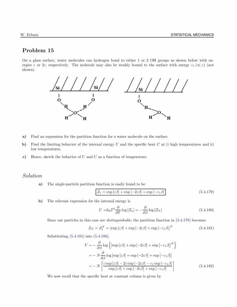
W. Erbsen STATISTICAL MECHANICS
Problem 15
On a glass surface, water molecules can hydrogen bond to either 1 or 2 OH groups as shown below with en-ergies ε or 2ε, respectively. The molecule may also be weakly bound to the surface with energy ε1 ( ε) (notshown).
a) Find an expression for the partition function for a water molecule on the surface.
b) Find the limiting behavior of the internal energy U and the specific heat C at i) high temperatures and ii)low temperatures.
c) Hence, sketch the behavior of U and C as a function of temperature.
Solution
a) The single-particle partition function is easily found to be
Z1 = exp [εβ] + exp [−2εβ] + exp [−ε1β] (5.4.179)
b) The relevant expression for the internal energy is
U =kBT2 ∂
∂Tlog [Zn] = − ∂
∂βlog [ZN ] (5.4.180)
Since our particles in this case are distinguishable, the partition function in (5.4.179) becomes
ZN = ZN1 = [exp [εβ] + exp [−2εβ] + exp [−ε1β]]N (5.4.181)
Substituting (5.4.181) into (5.4.180),
U = − ∂
∂βlog
[exp [εβ] + exp [−2εβ] + exp [−ε1β]]N
= −N∂
∂βlog [exp [εβ] + exp [−2εβ] + exp [−ε1β]]
= −N
[ε exp [εβ] − 2ε exp [−2εβ] − ε1 exp [−ε1β]
exp [εβ] + exp [−2εβ] + exp [−ε1β]
](5.4.182)
We now recall that the specific heat at constant volume is given by
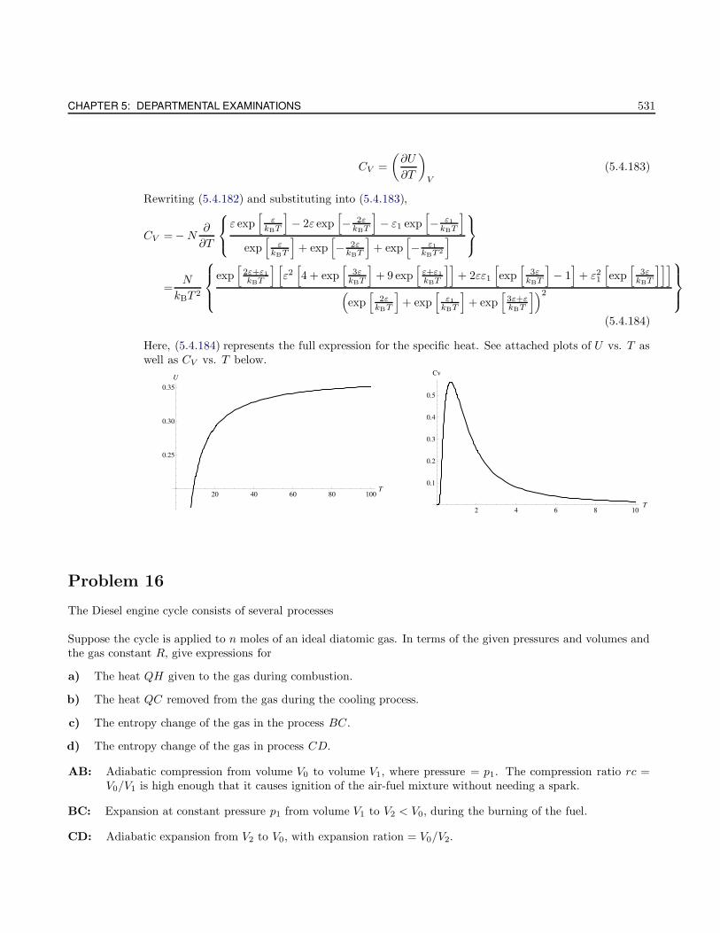
CHAPTER 5: DEPARTMENTAL EXAMINATIONS 531
CV =
(∂U
∂T
)
V
(5.4.183)
Rewriting (5.4.182) and substituting into (5.4.183),
CV = −N∂
∂T
ε exp
[ε
kBT
]− 2ε exp
[− 2ε
kBT
]− ε1 exp
[− ε1
kBT
]
exp[
εkBT
]+ exp
[− 2ε
kBT
]+ exp
[− ε1
kBT 2
]
=N
kBT 2
exp[
2ε+ε1
kBT
] [ε2[4 + exp
[3ε
kBT
]+ 9 exp
[ε+ε1
kBT
]]+ 2εε1
[exp
[3ε
kBT
]− 1]
+ ε21
[exp
[3ε
kBT
]]]
(exp
[2ε
kBT
]+ exp
[ε1
kBT
]+ exp
[3ε+εkBT
])2
(5.4.184)
Here, (5.4.184) represents the full expression for the specific heat. See attached plots of U vs. T aswell as CV vs. T below.
20 40 60 80 100T
0.25
0.30
0.35
U
2 4 6 8 10T
0.1
0.2
0.3
0.4
0.5
Cv
Problem 16
The Diesel engine cycle consists of several processes
Suppose the cycle is applied to n moles of an ideal diatomic gas. In terms of the given pressures and volumes andthe gas constant R, give expressions for
a) The heat QH given to the gas during combustion.
b) The heat QC removed from the gas during the cooling process.
c) The entropy change of the gas in the process BC.
d) The entropy change of the gas in process CD.
AB: Adiabatic compression from volume V0 to volume V1, where pressure = p1. The compression ratio rc =V0/V1 is high enough that it causes ignition of the air-fuel mixture without needing a spark.
BC: Expansion at constant pressure p1 from volume V1 to V2 < V0, during the burning of the fuel.
CD: Adiabatic expansion from V2 to V0, with expansion ration = V0/V2.
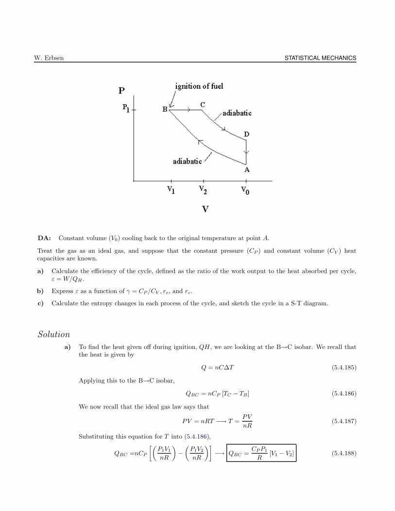
W. Erbsen STATISTICAL MECHANICS
DA: Constant volume (V0) cooling back to the original temperature at point A.
Treat the gas as an ideal gas, and suppose that the constant pressure (CP ) and constant volume (CV ) heatcapacities are known.
a) Calculate the efficiency of the cycle, defined as the ratio of the work output to the heat absorbed per cycle,ε = W/QH .
b) Express ε as a function of γ = CP/CV , re, and rc.
c) Calculate the entropy changes in each process of the cycle, and sketch the cycle in a S-T diagram.
Solution
a) To find the heat given off during ignition, QH , we are looking at the B→C isobar. We recall thatthe heat is given by
Q = nC∆T (5.4.185)
Applying this to the B→C isobar,
QBC = nCP [TC − TB ] (5.4.186)
We now recall that the ideal gas law says that
PV = nRT −→ T =PV
nR(5.4.187)
Substituting this equation for T into (5.4.186),
QBC =nCP
[(P1V1
nR
)−(P1V2
nR
)]−→ QBC =
CPP1
R[V1 − V2] (5.4.188)
CHAPTER 5: DEPARTMENTAL EXAMINATIONS 533
b) We now wish to find the heat QC removed during the cooling process, which along the D→Aisochor. The process is very much the same as in the last part, adopting (5.4.186) for our purposes,
QDA = nCV [TA − TD] (5.4.189)
And substituting (5.4.187) into (5.4.189),
QDA = nCV
[(PDV0
nR
)−(PAV0
nR
)]−→ QDA =
CV V0
R[PD − PA] (5.4.190)
c) Now we want to calculate the change in entropy along B→C. We first recall that the entropy isdefined by
∆S =Q
T(5.4.191)
Substituting (5.4.188) into (5.4.191),
∆S =CPP1
RT[V1 − V2] (5.4.192)
And also that the specific heat at constant pressure is
CP = T∂S
∂T(5.4.193)
Treating (5.4.193) like a differential equation,
1
CPdS =
1
TdT −→ S
CP= log
[V2
V1
](5.4.194)
Solving (5.4.194) for S,
S = CP log
[V2
V1
](5.4.195)
d) To find the change in entropy along the isochore D→A, we can go ahead and use (5.4.195) and saythat
S = CV log
[V0
V0
]−→ S = 0 (5.4.196)
e) We are now asked to find the efficiency of the entire cycle, which is given as ε = W/QH . We alsorecall that W = Qin −Qout, so that in our case, the efficiency is given by
ε =QBC −QDA
QBC
=
(CP P1
R [V1 − V2])−(
CV V0
R [PD − PA])
(CP P1
R [V1 − V2])
Which leads us to
ε =CPP1 [V1 − V2] −CV V0 [PD − PA]
CPP1 [V1 − V2]
W. Erbsen STATISTICAL MECHANICS
f ) We now wish to rewrite ε in terms of some new variables, which are
γ =CP
CV, re =
V0
V2, rc =
V0
V1
The result is
ε = 1 − 1
P1γ
[PD − PA
1/rc − 1/re
]−→ ε = 1 − 1
P1γ
[PD − PA
rc − re
]rcre
g) The entropy for both cycles are
∆SBC = ∆SDA = CP log
[V2
V1
], ∆SAB = ∆SCD = 0
And the net change in entropy is of course
∆Snet = 0
Problem 17
A classical monatomic ideal gas of N particles (each of mass m) is confined to a cylinder of radius r and in-finite height. A gravitational field points along the axis of the cylinder downwards.
a) Determine the Helmholtz energy A.
b) Find the internal energy U and the specific heat CV .
c) Why is CV 6= 3/2Nk?
Solution
a) There are two components of energy in this system: kinetic (p2/2m) and potential (mgh). TheHamiltonian for this system is then
H =p2
2m+mgz
=p2
x + p2y + p2
z
2m+mgz (5.4.197)
While the single-particle partition function takes the form
Z1 =1
h3
∫ ∫exp
[− H
kBT
]d3pd3r
(5.4.198)
Substituting our Hamiltonian from (5.4.197) into the partition function from (5.4.198) yields
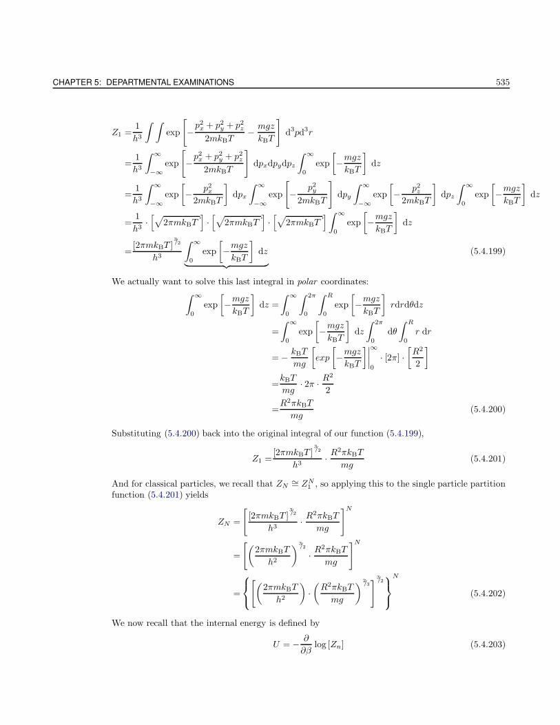
CHAPTER 5: DEPARTMENTAL EXAMINATIONS 535
Z1 =1
h3
∫ ∫exp
[−p2
x + p2y + p2
z
2mkBT− mgz
kBT
]d3pd3r
=1
h3
∫ ∞
−∞exp
[−p2
x + p2y + p2
z
2mkBT
]dpxdpydpz
∫ ∞
0
exp
[−mgzkBT
]dz
=1
h3
∫ ∞
−∞exp
[− p2
x
2mkBT
]dpx
∫ ∞
−∞exp
[−
p2y
2mkBT
]dpy
∫ ∞
−∞exp
[− p2
z
2mkBT
]dpz
∫ ∞
0
exp
[−mgzkBT
]dz
=1
h3·[√
2πmkBT]·[√
2πmkBT]·[√
2πmkBT] ∫ ∞
0
exp
[−mgzkBT
]dz
=[2πmkBT ]
3/2
h3
∫ ∞
0
exp
[−mgzkBT
]dz
︸ ︷︷ ︸(5.4.199)
We actually want to solve this last integral in polar coordinates:∫ ∞
0
exp
[−mgzkBT
]dz =
∫ ∞
0
∫ 2π
0
∫ R
0
exp
[−mgzkBT
]rdrdθdz
=
∫ ∞
0
exp
[−mgzkBT
]dz
∫ 2π
0
dθ
∫ R
0
r dr
= − kBT
mg
[exp
[−mgzkBT
]∣∣∣∣∞
0
· [2π] ·[R2
2
]
=kBT
mg· 2π · R
2
2
=R2πkBT
mg(5.4.200)
Substituting (5.4.200) back into the original integral of our function (5.4.199),
Z1 =[2πmkBT ]
3/2
h3· R
2πkBT
mg(5.4.201)
And for classical particles, we recall that ZN∼= ZN
1 , so applying this to the single particle partitionfunction (5.4.201) yields
ZN =
[[2πmkBT ]
3/2
h3· R
2πkBT
mg
]N
=
[(2πmkBT
h2
)3/2
· R2πkBT
mg
]N
=
[(2πmkBT
h2
)·(R2πkBT
mg
) 2/3]3/2
N
(5.4.202)
We now recall that the internal energy is defined by
U = − ∂
∂βlog [Zn] (5.4.203)
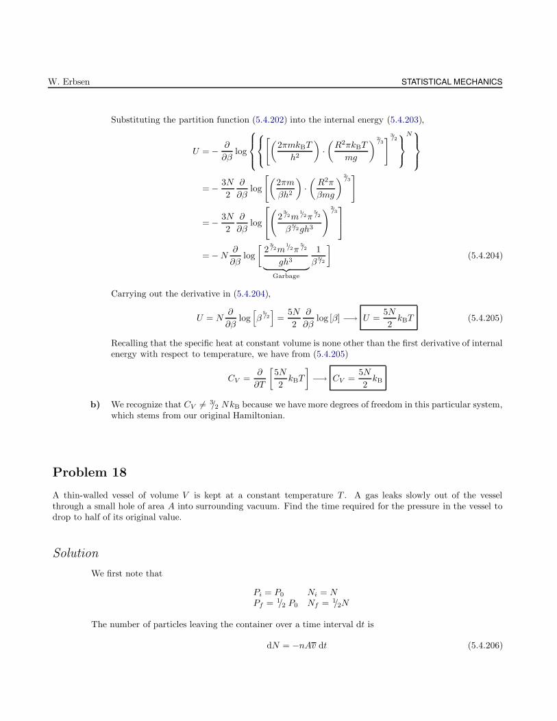
W. Erbsen STATISTICAL MECHANICS
Substituting the partition function (5.4.202) into the internal energy (5.4.203),
U = − ∂
∂βlog
[(2πmkBT
h2
)·(R2πkBT
mg
) 2/3]3/2
N
= − 3N
2
∂
∂βlog
[(2πm
βh2
)·(R2π
βmg
) 2/3]
= − 3N
2
∂
∂βlog
(
23/2m
1/2π5/2
β 5/2gh3
)2/3
= −N∂
∂βlog
[2
3/2m1/2π
5/2
gh3
︸ ︷︷ ︸Garbage
1
β 5/2
](5.4.204)
Carrying out the derivative in (5.4.204),
U = N∂
∂βlog[β
5/2]
=5N
2
∂
∂βlog [β] −→ U =
5N
2kBT (5.4.205)
Recalling that the specific heat at constant volume is none other than the first derivative of internalenergy with respect to temperature, we have from (5.4.205)
CV =∂
∂T
[5N
2kBT
]−→ CV =
5N
2kB
b) We recognize that CV 6= 3/2 NkB because we have more degrees of freedom in this particular system,which stems from our original Hamiltonian.
Problem 18
A thin-walled vessel of volume V is kept at a constant temperature T . A gas leaks slowly out of the vesselthrough a small hole of area A into surrounding vacuum. Find the time required for the pressure in the vessel todrop to half of its original value.
Solution
We first note that
Pi = P0 Ni = NPf = 1/2 P0 Nf = 1/2N
The number of particles leaving the container over a time interval dt is
dN = −nAv dt (5.4.206)
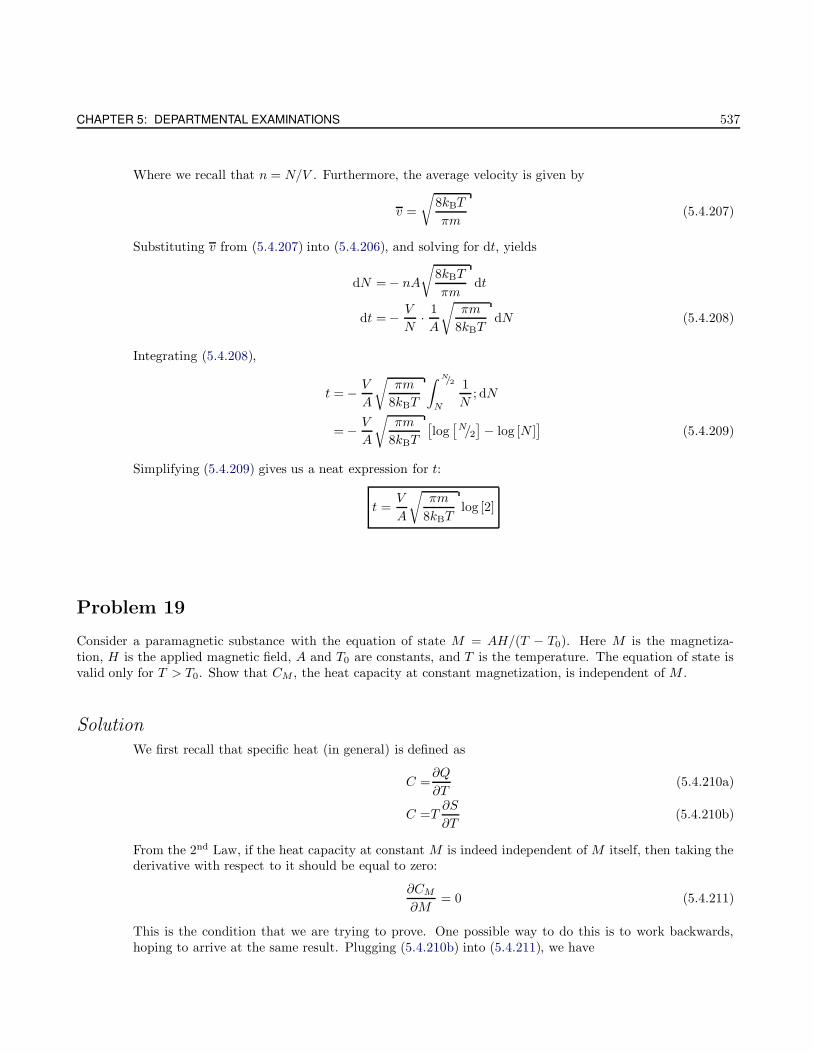
CHAPTER 5: DEPARTMENTAL EXAMINATIONS 537
Where we recall that n = N/V . Furthermore, the average velocity is given by
v =
√8kBT
πm(5.4.207)
Substituting v from (5.4.207) into (5.4.206), and solving for dt, yields
dN = − nA
√8kBT
πmdt
dt = − V
N· 1
A
√πm
8kBTdN (5.4.208)
Integrating (5.4.208),
t = − V
A
√πm
8kBT
∫ N/2
N
1
N; dN
= − V
A
√πm
8kBT
[log[
N/2]− log [N ]
](5.4.209)
Simplifying (5.4.209) gives us a neat expression for t:
t =V
A
√πm
8kBTlog [2]
Problem 19
Consider a paramagnetic substance with the equation of state M = AH/(T − T0). Here M is the magnetiza-tion, H is the applied magnetic field, A and T0 are constants, and T is the temperature. The equation of state isvalid only for T > T0. Show that CM , the heat capacity at constant magnetization, is independent of M .
Solution
We first recall that specific heat (in general) is defined as
C =∂Q
∂T(5.4.210a)
C =T∂S
∂T(5.4.210b)
From the 2nd Law, if the heat capacity at constant M is indeed independent of M itself, then taking thederivative with respect to it should be equal to zero:
∂CM
∂M= 0 (5.4.211)
This is the condition that we are trying to prove. One possible way to do this is to work backwards,hoping to arrive at the same result. Plugging (5.4.210b) into (5.4.211), we have
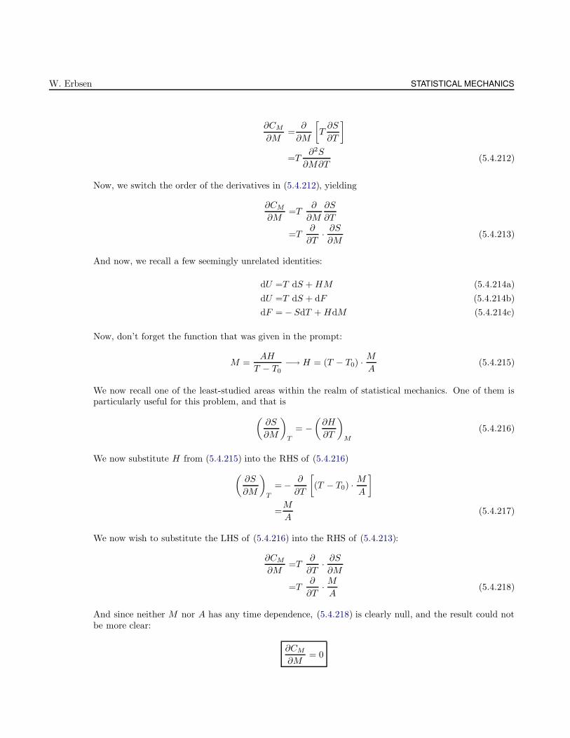
W. Erbsen STATISTICAL MECHANICS
∂CM
∂M=
∂
∂M
[T∂S
∂T
]
=T∂2S
∂M∂T(5.4.212)
Now, we switch the order of the derivatives in (5.4.212), yielding
∂CM
∂M=T
∂
∂M
∂S
∂T
=T∂
∂T· ∂S∂M
(5.4.213)
And now, we recall a few seemingly unrelated identities:
dU =T dS +HM (5.4.214a)
dU =T dS + dF (5.4.214b)
dF = − SdT +HdM (5.4.214c)
Now, don’t forget the function that was given in the prompt:
M =AH
T − T0−→ H = (T − T0) ·
M
A(5.4.215)
We now recall one of the least-studied areas within the realm of statistical mechanics. One of them isparticularly useful for this problem, and that is
(∂S
∂M
)
T
= −(∂H
∂T
)
M
(5.4.216)
We now substitute H from (5.4.215) into the RHS of (5.4.216)
(∂S
∂M
)
T
= − ∂
∂T
[(T − T0) ·
M
A
]
=M
A(5.4.217)
We now wish to substitute the LHS of (5.4.216) into the RHS of (5.4.213):
∂CM
∂M=T
∂
∂T· ∂S∂M
=T∂
∂T· MA
(5.4.218)
And since neither M nor A has any time dependence, (5.4.218) is clearly null, and the result could notbe more clear:
∂CM
∂M= 0
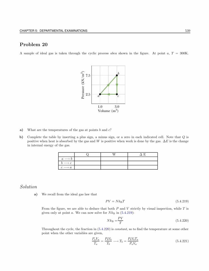
CHAPTER 5: DEPARTMENTAL EXAMINATIONS 539
Problem 20
A sample of ideal gas is taken through the cyclic process abca shown in the figure. At point a, T = 300K.
a) What are the temperatures of the gas at points b and c?
b) Complete the table by inserting a plus sign, a minus sign, or a zero in each indicated cell. Note that Q ispositive when heat is absorbed by the gas and W is positive when work is done by the gas. ∆E is the changein internal energy of the gas.
Q W ∆ E
a −→ bb −→ c
c −→ a
Solution
a) We recall from the ideal gas law that
PV = NkBT (5.4.219)
From the figure, we are able to deduce that both P and V strictly by visual inspection, while T isgiven only at point a. We can now solve for NkB in (5.4.219):
NkB =PV
T(5.4.220)
Throughout the cycle, the fraction in (5.4.220) is constant, so to find the temperature at some otherpoint when the other variables are given,
PaVa
Ta=PbVb
Tb−→ Tb =
PbVbTa
PaVa(5.4.221)
W. Erbsen STATISTICAL MECHANICS
Plugging in the appropriate values into (5.4.221),
Tb =
(7.5× 10³ N ·m2
) (3.0 m3
)(300 K)
(2.5 × 10³ N · m2) (1.0 m3)−→ Tb = 2700 K
We can repeat the same process to find Tc by making a change of variables from b→ c:
Tc =PcVcTa
PaVa(5.4.222)
And substituting in the correct values into (5.4.222), we have
Tc =
(2.5× 10³ N · m2
) (3.0 m3
)(300 K)
(2.5× 10³ N ·m2) (1.0 m3)−→ Tc = 900 K
b) We note that Q is positive when heat is absorbed, while W is positive when work is done by thegas. Accordingly,
From ∆t Q Wa → b ↑ ↑ ↑b → c ↓ ↓ =c → a ↓ ↑ ↓
Problem 21
A sample of helium gas inside a cylinder terminated with a piston doubles its volume from Vi = 1m3 to Vf = 2m3.During this process the pressure and volume are related by PV
6/5 = A = constant. Assume that the product PValways equals 2/3U , where U is the internal energy.
a) What is the change in energy of the gas?
b) What is the change in entropy of the gas?
c) How much heat was added to or removed from the gas?
Solution
a) Given that the original formula PV6/5 = A, we can solve for P before and after this expansion:
Pi =A
V6/5
i
, Pf =A
V6/5
f
And the change in energy can be found using the second given expression,
PV =2
3U −→ U =
3
2PV (5.4.223)
And so the change in energy, ∆U , can be found by
∆U =3
2(PfVf − PiVi)
CHAPTER 5: DEPARTMENTAL EXAMINATIONS 541
=3
2
(A
V6/5
f
Vf − A
V6/5
i
Vi
)
=3
2A
(1
V1/5
f
− 1
V1/5
i
)(5.4.224)
Substituting in the appropriate values into (5.4.224),
∆U =3
2A
(1
(2 m3)1/5
− 1
(1 m3)1/5
)(5.4.225)
b) To find the change in entropy of the gas, we first recall that a common form of the first law ofthermodynamics is
dU = T dS − P dV (5.4.226)
Solving (5.4.226) for dS,
dS =1
TdU +
P
TdV (5.4.227)
We now recall from the ideal gas law, and also from the information given in the problem, that
PV = NkBT =2
3U −→ U =
3
2NkBT (5.4.228a)
−→ T =2
3
U
NkB(5.4.228b)
−→ P =NkBT
V=
2
3
U
V(5.4.228c)
Substituting (5.4.228a)-(5.4.228c) into (5.4.227),
dS =
(3
2
NkB
U
)dU +
1
T
(NkBT
V
)dV
=3
2NkB
(1
UdU
)+ nkB
(1
VdV
)(5.4.229)
Integrating, (5.4.229) becomes
S =3
2NkB [logU |Uf
Ui+ nkB [logV |V
f
Vi
=3
2NkB log
[Uf
Ui
]+NkB log
[Vf
Vi
](5.4.230)
And we now innocently recall that
Uf =3
2A
1
(2 m3)1/5
=3
2A
1
V1/5
f
(5.4.231a)
Ui =3
2A
1
(1 m3)1/5
=3
2A
1
V1/5
i
(5.4.231b)
And substituting (5.4.231a) and (5.4.231b) into S from (5.4.230),
W. Erbsen STATISTICAL MECHANICS
S =3
2NkB log
V
−1/5f
V−1/5
i
+NkB log
[Vf
Vi
]
=3
10NkB log
[Vi
Vf
]+NkB log
[Vf
Vi
]
=7
10NkB log
[Vf
Vi
](5.4.232)
Substituting the appropriate values into (5.4.232), we are left with
S =7
10NkB log [2]
c) We first recall that
dQ = dW + dU (5.4.233)
To find out what W is in (5.4.233), we recall that work is defined as W =∫PdV . Also remembering
that PV6/5 = A→ P = AV −6/5 , so we have
W =A
∫ Vf
Vi
V −6/5 dV
= − A · 5[
1
V1/5
∣∣∣∣Vf
Vi
= − A · 5(
1
V1/5
f
− 1
V1/5
i
)(5.4.234)
Now, substituting ∆U from (5.4.225) and W from (5.4.234) into (5.4.233), we have
Q = −A · 5(
1
V1/5
f
− 1
V1/5
i
)+
3
2· A(
1
V1/5
f
− 1
V1/5
i
)
= − 7
2A
(1
V1/5
f
− 1
V1/5
i
)
And with the given values, this becomes
Q =7
2A
(1
(1 m3)1/5
− 1
(2 m3)1/5
)
Problem 24
An arbitrary network of resistors, capacitors, and inductors is in thermal equilibrium at temperature T . There areno sources in the network.
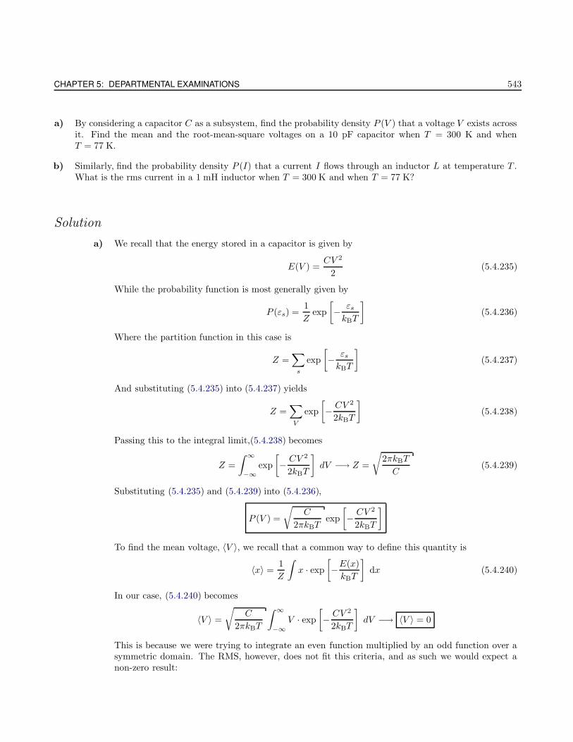
CHAPTER 5: DEPARTMENTAL EXAMINATIONS 543
a) By considering a capacitor C as a subsystem, find the probability density P (V ) that a voltage V exists acrossit. Find the mean and the root-mean-square voltages on a 10 pF capacitor when T = 300 K and whenT = 77 K.
b) Similarly, find the probability density P (I) that a current I flows through an inductor L at temperature T .What is the rms current in a 1 mH inductor when T = 300 K and when T = 77 K?
Solution
a) We recall that the energy stored in a capacitor is given by
E(V ) =CV 2
2(5.4.235)
While the probability function is most generally given by
P (εs) =1
Zexp
[− εs
kBT
](5.4.236)
Where the partition function in this case is
Z =∑
s
exp
[− εs
kBT
](5.4.237)
And substituting (5.4.235) into (5.4.237) yields
Z =∑
V
exp
[− CV 2
2kBT
](5.4.238)
Passing this to the integral limit,(5.4.238) becomes
Z =
∫ ∞
−∞exp
[− CV 2
2kBT
]dV −→ Z =
√2πkBT
C(5.4.239)
Substituting (5.4.235) and (5.4.239) into (5.4.236),
P (V ) =
√C
2πkBTexp
[− CV 2
2kBT
]
To find the mean voltage, 〈V 〉, we recall that a common way to define this quantity is
〈x〉 =1
Z
∫x · exp
[−E(x)
kBT
]dx (5.4.240)
In our case, (5.4.240) becomes
〈V 〉 =
√C
2πkBT
∫ ∞
−∞V · exp
[− CV 2
2kBT
]dV −→ 〈V 〉 = 0
This is because we were trying to integrate an even function multiplied by an odd function over asymmetric domain. The RMS, however, does not fit this criteria, and as such we would expect anon-zero result:
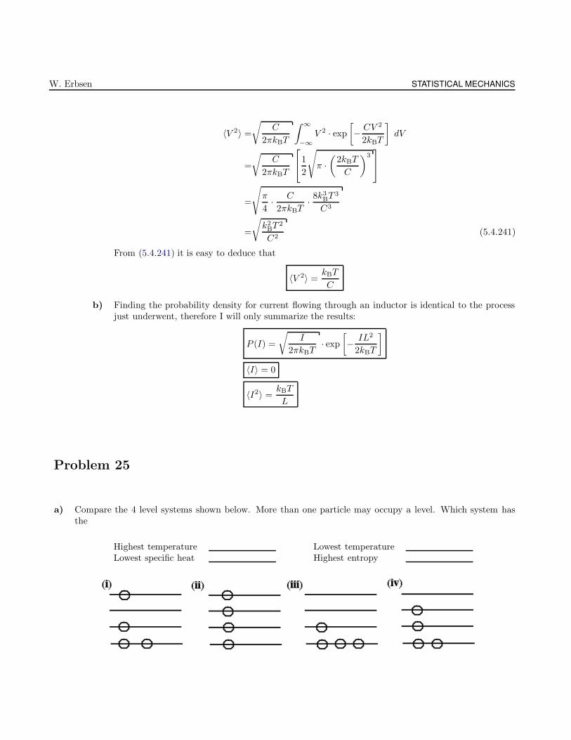
W. Erbsen STATISTICAL MECHANICS
〈V 2〉 =
√C
2πkBT
∫ ∞
−∞V 2 · exp
[− CV 2
2kBT
]dV
=
√C
2πkBT
1
2
√
π ·(
2kBT
C
)3
=
√π
4· C
2πkBT· 8k3
BT3
C3
=
√k2BT
2
C2(5.4.241)
From (5.4.241) it is easy to deduce that
〈V 2〉 =kBT
C
b) Finding the probability density for current flowing through an inductor is identical to the processjust underwent, therefore I will only summarize the results:
P (I) =
√I
2πkBT· exp
[− IL2
2kBT
]
〈I〉 = 0
〈I2〉 =kBT
L
Problem 25
a) Compare the 4 level systems shown below. More than one particle may occupy a level. Which system hasthe
Highest temperature Lowest temperatureLowest specific heat Highest entropy
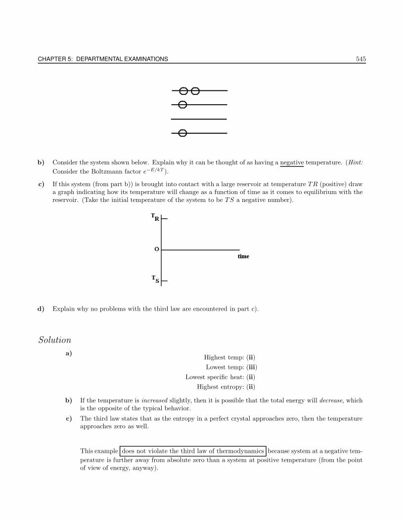
CHAPTER 5: DEPARTMENTAL EXAMINATIONS 545
b) Consider the system shown below. Explain why it can be thought of as having a negative temperature. (Hint:
Consider the Boltzmann factor e−E/kT ).
c) If this system (from part b)) is brought into contact with a large reservoir at temperature TR (positive) drawa graph indicating how its temperature will change as a function of time as it comes to equilibrium with thereservoir. (Take the initial temperature of the system to be TS a negative number).
d) Explain why no problems with the third law are encountered in part c).
Solution
a)Highest temp: (ii)
Lowest temp: (iii)
Lowest specific heat: (ii)
Highest entropy: (ii)
b) If the temperature is increased slightly, then it is possible that the total energy will decrease, whichis the opposite of the typical behavior.
c) The third law states that as the entropy in a perfect crystal approaches zero, then the temperatureapproaches zero as well.
This example does not violate the third law of thermodynamics because system at a negative tem-
perature is further away from absolute zero than a system at positive temperature (from the pointof view of energy, anyway).
W. Erbsen STATISTICAL MECHANICS
Problem 26
Equipartition. A classical harmonic oscillator
H =p2
2m+Kq2
2(5.4.242)
is in thermal contact with a heat bath at temperature T . Calculate the partition function for the oscillator in thecanonical ensemble and show explicitly that
〈E〉 = kBT, and 〈(E − 〈E〉)2〉 = (kBT )2
(5.4.243)
Solution
We first recall that the single-particle partition function is given by
Z1 =1
h3
∫ ∫exp [−βH] d3pd3q (5.4.244)
However, in our case we are assuming that the Hamiltonian is only in 1-D, so that substituting ourHamiltonian from (5.4.242) into (5.4.244), we have
Z1 =1
h
∫ ∫exp
[−β(p2
2m+kq2
2
)]dpdq
=1
h
∫ ∞
−∞exp
[− p2
2mkBT
]dp
∫ ∞
−∞exp
[Kq2
2
]dq
=1
h
(√2mπkBT
)(√2πkBT
K
)
=2πkBT
h
√m
K(5.4.245)
We now recall that the internal energy, 〈E〉, is defined by
〈E〉 = − ∂
∂βlogZ1 (5.4.246)
Rearranging (5.4.245) and substituting into (5.4.246), we have
〈E〉 = − ∂
∂βlog
[2π
βh
√m
K
]−→ 〈E〉 = kBT (5.4.247)
Now, we recall that
〈(E − 〈E〉)2〉 = 〈E2〉 − 〈E〉2 (5.4.248)
And we can also express 〈E〉 in yet another way
〈E〉 =1
Z1
∫ ∫E · exp [−βH] dpdq −→ 〈E〉 = kBT (5.4.249)
CHAPTER 5: DEPARTMENTAL EXAMINATIONS 547
As before, We can extend this to find 〈E2〉, however, and (5.4.249) becomes
〈E2〉 =1
Z1
∫ ∫E2 exp [−βH] dpdq (5.4.250)
And now, seemingly arbitrarily, we take the first derivative of 〈E〉 with respect to β in (5.4.247):
∂
∂β〈E〉 =
∂
∂β
1
β= − 1
β2(5.4.251)
And now, stay with me here, we wish to do the same thing for the primary expression in (5.4.249):
∂
∂β〈E〉 =
∂
∂β
[1
Z1
∫ ∫E · exp [−βH] dpdq
](5.4.252)
Recognizing that Z1 has a dependence on β, we continue with (5.4.252), yielding
∂
∂β〈E〉 =
1
Z1
[∂
∂β
∫ ∫E · exp [−βH] dpdq
]+
∫ ∫E · exp [−βH] dpdq
[∂
∂β
1
Z1
]
=1
Z1
∫ ∫E2 · exp [−βH] dpdq +
∫ ∫E · exp [−βH] dpdq
[∂
∂β
1
Z1︸ ︷︷ ︸
](5.4.253)
Let’s take a closer look at the underbraced term in (5.4.253), using the value of Z1 found in (5.4.245):
∂
∂β
1
Z1=
∂
∂β
[hβ
2π
√K
m
]⇒ h
2π
√K
m(5.4.254)
Substituting (5.4.254) back in to (5.4.253),
∂
∂β〈E〉 =
1
Z1
∫ ∫E2 · exp [−βH] dpdq +
h
2π
√K
m
∫ ∫E · exp [−βH] dpdq (5.4.255)
Inserting in to (5.4.255) our expression for Z1 found in (5.4.245),
∂
∂β〈E〉 =
h
2πkBT
√K
m
∫ ∫E2 · exp [−βH] dpdq +
h
2π
√K
m
∫ ∫E · exp [−βH] dpdq
︸ ︷︷ ︸(5.4.256)
Let us know rewrite the underbraced term in (5.4.256):
h
2π
√K
m
∫ ∫E · exp [−βH] dpdq =
h
2π
√K
m· Z1〈E〉
=h
2π
√K
m·[2πkBT
h
√m
K
]〈E〉
=1
β〈E〉 (5.4.257)
Plugging (5.4.257) back into (5.4.256),
∂
∂β〈E〉 =
1
Z1
∫ ∫E2 · exp [−βH] dpdq
︸ ︷︷ ︸+
1
β〈E〉 (5.4.258)
W. Erbsen STATISTICAL MECHANICS
We immediately recognize the underbraced term to be none other than our good friend 〈E2〉. Using thisknowledge, we can now rewrite (5.4.258),
∂
∂β〈E〉 =〈E2〉 +
1
β〈E〉
Rearranging this a bit,
〈E2〉 =1
β〈E〉 − ∂
∂β〈E〉
=1
β
(1
β
)− ∂
∂β
(1
β
)
=1
β2+
1
β2
=2
β2(5.4.259)
Substituting (5.4.247) and (5.4.259) into (5.4.248),
〈E2〉 − 〈E〉2 =2
β2− 1
β2−→ 〈E2〉 − 〈E〉2 = (kBT )2
Problem 27
Consider two single-particle states and two particles. Calculate the entropy of this system when the particleshave the following statistics:
a) Maxwell-Boltzmann (i.e. classical)
b) Bose-Einstein
c) Fermi-Dirac
d) If two particles of mass m are confined to a box of volume V , approximately what temperature do classicalstatistics lose their validity?
Solution
a) We first recall how the entropy depends on the multiplicity
S = kB log [Ω] (5.4.260)
We first need to know what the multiplicity, Ω is before we can use this tool though. The multi-plicity refers to the number of available states in the system. It’s as simple as that.
For Maxwell-Boltzmann statistics, we recognize that this is a classical system, and both particlesmay occupy any of the states available with no restrictions what-so-ever:
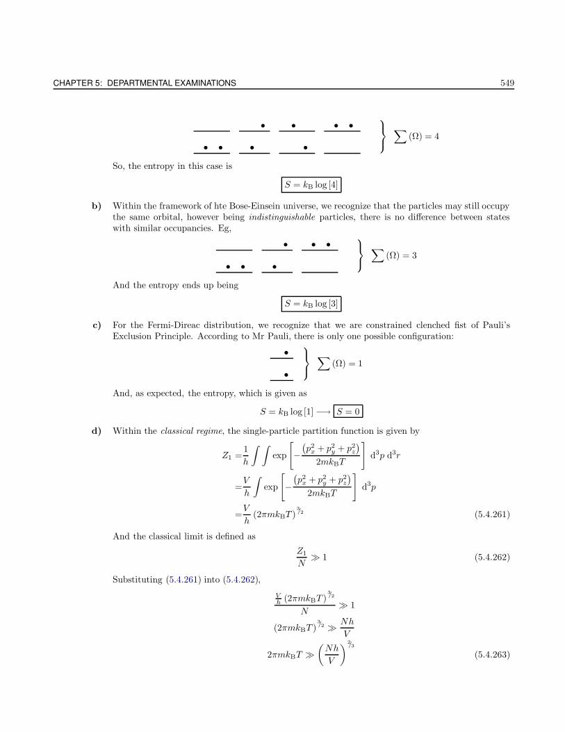
CHAPTER 5: DEPARTMENTAL EXAMINATIONS 549
• • • •
• • • •
∑(Ω) = 4
So, the entropy in this case is
S = kB log [4]
b) Within the framework of hte Bose-Einsein universe, we recognize that the particles may still occupythe same orbital, however being indistinguishable particles, there is no difference between stateswith similar occupancies. Eg,
• • •
• • •
∑(Ω) = 3
And the entropy ends up being
S = kB log [3]
c) For the Fermi-Direac distribution, we recognize that we are constrained clenched fist of Pauli’sExclusion Principle. According to Mr Pauli, there is only one possible configuration:
•
•
∑(Ω) = 1
And, as expected, the entropy, which is given as
S = kB log [1] −→ S = 0
d) Within the classical regime, the single-particle partition function is given by
Z1 =1
h
∫ ∫exp
[−(p2
x + p2y + p2
z
)
2mkBT
]d3p d3r
=V
h
∫exp
[−(p2
x + p2y + p2
z
)
2mkBT
]d3p
=V
h(2πmkBT )
3/2 (5.4.261)
And the classical limit is defined as
Z1
N 1 (5.4.262)
Substituting (5.4.261) into (5.4.262),
Vh (2πmkBT )
3/2
N 1
(2πmkBT )3/2 Nh
V
2πmkBT (Nh
V
)2/3
(5.4.263)
W. Erbsen STATISTICAL MECHANICS
From (5.4.263), it is easy to see that the condition is
T 1
2πmkB
(Nh
V
) 2/3
Problem 28
A zipper has N links; each link has a state in which it is closed with energy 0 and a state in which it is open withenergy ε. We require, however, that the zipper can only unzip from the left end, and that the link number, s, canonly open if all links to the left (1, 2, ..., s− 1) are already open.
a) Show that the partition function can be summed in the form:
QN =1 − exp [−(N + 1)βε]
1 − exp[−βε] (5.4.264)
b) In the limit ε kT , find the average number of open links.
The above model is a very simplified model of the unwinding of two-stranded DNA molecules.
Solution
Ooooh the zipper problem. I zip you so much.
a) The standard form of the single-particle partition function is
Z1 =
∞∑
s=0
exp
[− εs
kBT
](5.4.265)
Because the “particles” are distinguishable, then we can gain the full partition from (5.4.265) quiteeasily
Zs =
∞∑
s=0
exp
[− εs
kBT
]s
(5.4.266)
We now take a field trip. Let’s take a close look at the following series:
N∑
s=0
xs = 1 + x+ x2 + x3 + ...+ xN (5.4.267)
We now multiply both sides of (5.4.267) by x. This looks like
x
N∑
s=0
xs = x+ x2 + x3 + x4 + ...+ xN+1 (5.4.268)
We now take (5.4.267) and subtract from it (5.4.268). This yields
CHAPTER 5: DEPARTMENTAL EXAMINATIONS 551
(1 − x)
N∑
s=0
xs = 1 − xN+1 (5.4.269)
If we were to rearrange (5.4.269), then it would look like
N∑
s=0
xs =1 − xN+1
1 − x(5.4.270)
This exact sum is what we need in order to evaluate (5.4.266)!
Zs =1 − exp [− (N + 1) εβ]
1 − exp [−εβ](5.4.271)
b) In general, the way to find the average number of open links, we use the form
〈s〉 =1
Zs
N∑
s=0
s · exp[−sεβ] (5.4.272)
Now, notice that we can arrive at (5.4.272) if we are very tricky and take a derivative of the followingform:
〈s〉 =1
Zs
∂
∂ (εβ)
N∑
s=0
exp [−sεβ]
︸ ︷︷ ︸Zs
(5.4.273)
Rewriting (5.4.273) once more,
〈s〉 =1
Zs
∂
∂xZs (5.4.274)
Where I have made the temporary substitution x = εβ for convenience. Carrying out the firstderivative in (5.4.274),
∂
∂xZs =
∂
∂x
1 − exp [− (N + 1)x]
1 − exp [−x]
=1
1 − exp [−x]
[∂
∂x[1 − exp [− (N + 1)x]]
]+ [1 − exp [− (N + 1)x]]
[∂
∂x
1
1 − exp [−x]
]
=1
1 − exp [−x] [(N + 1) exp [−(N + 1)x]] − [1 − exp [−(N + 1)x]]
[exp [−x]
(1 − exp [−x])2
]
=(N + 1)exp [−(N + 1)x]
1 − exp [−x] − exp [−x][
1 − exp [−(N + 1)x]
(1 − exp [−x])2
]
=(N + 1)exp [−(N + 1)x]
1 − exp [−x] − exp [−x](1 − exp [−x])2
+exp [−x] exp [−(N + 1)x]
(1 − exp [−x])2
=(N + 1)exp [−(N + 1)x]
1 − exp [−x] − 1
1 − exp [−x]
[− exp [−x]
1 − exp [−x] +exp [−(N + 1)x] exp [−x]
1 − exp [−x]
]
=1
1 − exp [−x]
[(N + 1) exp [−(N + 1)x] − exp [−x]
1 − exp [−x] +exp [−(N + 1)x] exp [−x]
1 − exp [−x]
]
W. Erbsen STATISTICAL MECHANICS
=1
1 − exp [−x]
[(N + 1) exp [−(N + 1)x] − exp [−x]
1 − exp [−(N + 1)x]
1 − exp [−x]
](5.4.275)
Where we note that the expression in brackets in (5.4.275) is none other than Zs. Rewriting,
∂
∂xZs =
1
1 − exp [−x] [(N + 1) exp [−(N + 1)x] − exp [−x]Zs] (5.4.276)
At this point we are ready to substitute (5.4.276) and (5.4.271) into (5.4.274):
〈s〉 =1
Zs· 1
1 − exp [−x] [(N + 1) exp [−(N + 1)x]− exp [−x]Zs]
=(N + 1) exp [−(N + 1)x]− exp [−x]
1 − exp [−x]
=(N + 1) exp [−(N + 1)x]
1 − exp [−x] − exp [−x]1 − exp [−x] (5.4.277)
Putting the numbers back in to (5.4.277) leads us to
〈s〉 =(N + 1) exp [−(N + 1)εβ]
1 − exp [−εβ]− exp [−εβ]
1 − exp [−εβ](5.4.278)
We are asked to evaluate the average number of open links from (5.4.278) given the followingstipulation:
ε kBT −→ εβ 1
If εβ 1, then all the exponential terms approach zero, and so the average number of open links is
〈s〉 = 0
Problem 29
a) Obtain the Van der Waals equation of state
(p+
N2a
V
)(V −Nb) = NkT (5.4.279)
by making the following two corrections to the ideal gas:
i) Use an “effective volume,” instead of the usual volume
ii) Include interactions in a mean field form. State clearly where the mean field assumptions come in.
b) What is the work done by the gas if it expands isothermally from V1 to V2 at some temperature T?
Solution
CHAPTER 5: DEPARTMENTAL EXAMINATIONS 553
a) The ideal gas law is, of course, given by
PV = NkBT (5.4.280)
Let’s apply ii) first to (5.4.280), where we are including interactions from the “mass field form.”
Mean field theory essentially consists of replacing all interactions attributed to any one body, withan average, or “effective” interaction.→ This reduces a complicated multi-body problem to an effectively single-body problem, whose
solutions are easier to find.
But what is the probability that two particles will be in the same place at the same time?→ The density (ρ = m/v) is sort of like a probability, in the sense that if the density is large, the
probability that two particles will try to be in the same space at the same time increases (thisprobability actually goes like P ∝ ρ2).
→ Think of two coins: if the probability that one is heads up is ρ, then the probability that theywill both be heads up is ρ2.
This adds an “effective pressure” term to (5.4.280). The addition of a new term indicates thatdue to the chance of spatially co-existing molecules, the pressure is actually more, proportional toseveral constants. Anyway, with this correction, (5.4.280) becomes
(P + aρ2
)V = NkBT (5.4.281)
Where the constant a is a proportionality constant, which depends on how much the particles in-teract with one another.
We now recall how we define the particle density :
ρ =N
V
Substituting this in to (5.4.281) yields(P + a
N2
V 2
)V = NkBT (5.4.282)
Next, we wish to address i), which is attributed to the “effective volume,” which basically meansthat the two particles cannot coexist at the same place at the same time.→ Therefore, the amount of space available for these molecules flying around is actually less then
the total volume of the container, by an amount proportional to the number of molecules present:
Veff = V −Nb (5.4.283)
Where b is the volume of the individual gas particle, and N is the number of particles in the volume.Therefore, substituting (5.4.283) into (5.4.282), we have
(P + a
N2
V 2
)(V −Nb) = NkBT (5.4.284)
W. Erbsen STATISTICAL MECHANICS
b) To find the work done by a gas which expands isothermally (constant temperature), from someinitial volume Vi to some final volume Vf , we must first recall that
W =
∫ Vf
Vi
P dV (5.4.285)
At this point, we solve (5.4.284) for P , which will subsequently be substituted into (5.4.285). Butfirst things first:
P =NkBT
V −Nb− aN2
V 2(5.4.286)
And now substituting (5.4.286) back into (5.4.285),
W =
∫ Vf
Vi
[NkBT
V −Nb− aN2
V 2
]dV
=NkBT
∫ Vf
Vi
1
V −NbdV − aN2
∫ Vf
Vi
1
V 2dV
=NkBT [log [V −Nb]|Vf
Vi− aN2
[− 1
V
∣∣∣∣Vf
Vi
=NkBT [log [Vf −Nb]− log [Vi −Nb]] + aN2
[1
Vf− 1
Vi
](5.4.287)
We can simplify (5.4.287) slightly, leaving us with
W = NkBT log
[Vf −Nb
Vi −Nb
]+ aN2
[1
Vf− 1
Vi
]
Problem 30
A quantum harmonic oscillator has energy levels En =(n+ 1/2
)~ω0, where n = 0, 1, 2, ... Treat this single oscilla-
tor to be a small system coupled to a heat bath at temperature T . What is the probability of finding the oscillatorin its nth quantum state?
Solution
The Quantum Harmonic Oscillator (or simply QHO, as we lovingly call it) has the following eigenenergies:
En =(n+ 1/2
)~ω (5.4.288)
And if we dutifully recall, the partition function is given by
Z =
∞∑
n=0
exp
[− En
kBT
](5.4.289)
CHAPTER 5: DEPARTMENTAL EXAMINATIONS 555
Now, we are interested in finding the QHO in some other state, let’s call it n′. How do we find this out?Well, we first recall that
P (En) =exp [−En/(kBT )]
Z(5.4.290)
Now let’s tailor it to our system in need:
P (E′n) =
exp [−E′n/(kBT )]
Z(5.4.291)
Now, we must find Z:
Z =
∞∑
n=0
exp
[−(n + 1/2
)~ω0
kBT
](5.4.292)
Now, the nth excited state is n′, and (5.4.291) becomes
P (E′n) =
exp[−(n′ + 1/2
)~ω0
]/(kBt)∑∞
n=0 exp [− (n+ 1/2) ~ω0/(kBT )]
=exp
[−(n′ + 1/2
)~ω0β
]∑∞
n=0 exp [− (n+ 1/2) ~ω0β]
= exp[−(n′ + 1/2
)~ω0β
]·
∞∑
n=0
exp[(n+ 1/2
)~ω0β
]
=exp[−n′~ω0β − 1/2~ω0β
]· exp
[1/2~ω0β
] ∞∑
n=0
exp [n~ω0β]
= exp[−n′~ω0β − 1/2~ω0β + 1/2~ω0β
]·
∞∑
n=0
exp [n~ω0β]
= exp [−n′~ω0β] ·∞∑
n=0
exp [n~ω0β] (5.4.293)
At this point we recall the following arcane summation identity
∞∑
n=0
ean =1
1− ea
Applying this to (5.4.293),
P (E′n) =
exp [−n′~ω0β]
1− exp [~ω0β]
Problem 31
The surface temperature of the sun is T0(= 5800o K); its radius is R(= 7 × 10⁸ m) while the radius of the
W. Erbsen STATISTICAL MECHANICS
Earth is r(= 6.37× 10⁶ m). The mean distance between the sun and Earth is L(= 1.5× 10¹³ m). In first approx-imation, one can assume that both the sun and the Earth absorb all electromagnetic radiation incident upon them.
Assume that Earth has reached a steady state at some temperature T .
a) Find an approximate expression for the temperature T of Earth in terms of the astronomical parametersmentioned above.
b) Calculate the temperature T numerically.
Solution
a) The Stefan-Boltzmann Law gives the total power that the Sun is emitting, and is given by
PS = 4πR2σT 40 (5.4.294)
Since the sun emits radiation in all directions, the Earth only absorbs a small fraction of the totaloutput, and depends on the cross sectional area of the Earth and the distance it is from the emitter.Quantitatively,
PE =PSA
4πL2
=PSπr2
4πL2
=PSr2
4L2(5.4.295)
As suggested in the prompt, if we assume in the first approximation that the Earth is a perfectabsorber, then (5.4.295) holds, and we can use (5.4.294) to come up with another expression whichdescribes the power absorbed by the Earth.
We start by slightly rewriting (5.4.294)
PE = 4πr2σT 4 (5.4.296)
At this point, we substitute both (5.4.294) and (5.4.296) into (5.4.295):
4πr2σT 4 = 4πR2σT 40 · r2
4L2−→ T 4 = T 4
0 · R2 · 1
4L2(5.4.297)
From (5.4.297) it is easy to see that
T = T0
√R
2L(5.4.298)
b) Substituting in the appropriate values into (5.4.298), we solve
T = 5800 K
√7 × 10⁸ m
2 (1.5× 10¹⁵) m−→ T = 28.017 K
CHAPTER 5: DEPARTMENTAL EXAMINATIONS 557
Problem 32
A 1.00 gram drop of water is supercooled to −5.00o C (remains in liquid state). Then suddenly and irreversiblyit freezes and becomes solid ice at the temperature of the surrounding air, 5.00o C. The specific heat of ice is2.220 J · g−1 · K, and of water is 4.136 J · g−1 · K, and the heat of fusion of water is 333 J · g−1.
a) How much heat leaves the drop as it freezes?
b) What is the change in entropy of the drop as it freezes?
Solution
m = 1.00 g
T1 = −5.00o Cw = 2.220 J · g−1 · KT2 = −5.00o Ci = 4.186 J · g−1 ·K
Lf = 3.333 J · g−1
a) Two equations that have been since long forgotten are
Q =mC∆T (5.4.299a)
Q =mLf (5.4.299b)
Where we recall that the heat, Q is the key quantity in all this. If a cup of ice is sitting in roomtemperature, then heat is entering the vessel, causing it to melt. If, however you have the same cupof ice cooled to exactly 32o F (remember, ice doesn’t normally freeze lower than this), and it startsto turn to water of the same temperature. The heat required to make this phase transition maynot contribute towards a change in ∆T , however energy is being applied because it takes energy toundergo a phase change.
In our case, the sample does not undergo any change in temperature, and the amount of heatthat leaves the drop is due only to the change of phase. Therefore, we only need to use (5.4.299b),and applying the appropriate constants, yields
Q = (1.00 g)(333 J · g−1
)−→ Q = 333 J (5.4.300)
b) A common form of entropy is
dS =∆Q
T(5.4.301)
And substituting in the appropriate values into (5.4.301), we have
S =333 J
273 − 5 K−→ S = 1.243 J ·K−1