WELL LOGGING LABORATORY TECHNICAL...
152
+ WELL LOGGING LABORATORY TECHNICAL REPORT NO. 33 October 2012 Department of Electrical Engineering Cullen College of Engineering University of Houston
Transcript of WELL LOGGING LABORATORY TECHNICAL...

+
WELL LOGGING LABORATORY
TECHNICAL REPORT NO. 33
October 2012
Department of Electrical Engineering
Cullen College of Engineering
University of Houston

Technical Report N
o. 33 University of H
ouston 2012

i
WELL LOGGING TECHNICAL REPORT NO. 33
October 2012
All rights reserved
Well Logging Laboratory Department of Electrical and Computer Engineering
University of Houston Houston, Texas 77204-4005
U. S. A.

ii
Research Staff Faculty Dr. Hezhu Yin, Adjunct Professor
Dr. Hanming Wang, Adjunct Professor
Dr. Donald Wilton, Professor
Dr. Ning Yuan, Research Assistant Professor
Dr. Richard Liu, Professor
Research Assistants
Jing Wang (Ph.D. Candidate)
Bo Gong (Ph.D. Candidate)
Pengfei Liu (Ph.D. Candidate)
Yinxi Zhang (Ph.D. Candidate)
Boyuan Yu (Ph.D. Candidate)
Fouad Shehab (Master Candidate)
Yajun Kong (M. S. Candidate)
Chang Ming Lin (M. S. Candidate)
Ziting Liu (M. S. Candidate)
Xiangyang Mu (Visiting Professor)

iii
Acknowledgment
The authors would like to acknowledge gratefully the financial support and the technical assistance which they have received from the following companies: BP
Chevron E & P Technology Company
ExxonMobil Upstream Research Company
Great Wall Drilling Company
Halliburton Energy Services
Saudi Aramco
Schlumberger Oilfield Services
Statoil
Weatherford

iv
TECHNICAL REPORT NO. 33 (2012)
Table of Contents
Research Staff ..................................................................................................................... ii
Acknowledgment ............................................................................................................... iii
Table of Contents ............................................................................................................... iv
CHAPTER 1 Application of Image Theory in Geo-Steering, by Jing Wang and Richard
Liu...........................................................................................................1-1
CHAPTER 2 Preliminary Study of Look-Ahead Resistivity Logging Tools, by Bo Gong
and Richard Liu…………………………………………………2-1
CHAPTER 3 Analysis of Pulsed Look Ahead Tools Using FDTD Method, by Boyuan
Yu and Richard Liu…………………………………..….......................3-1
CHAPTER 4 Dielectric Constant of Rocks Obtained by Using Micro-CT Images, by El
Emir Fouad Shehab and Richard Liu…………..………………..4-1
CHAPTER 5 Study of Array Dielectric Logging Tools, by Yinxi Zhang and Richard
Liu….…………….……………...…………………………………….5-1
APPENDIX A List of Theses and Dissertations…………………………………...…...A1
APPENDIX B List of Technical Paper Publications…………………………...………B1

The application of Image Theory in Geo-steering
1-1
CHAPTER 1
The Application of Image Theory in Geo-Steering
Abstract
Geo-steering is a real-time system used to control and adjust the direction of the drilling
bit in a horizontal or deviated well. One of the most challenging issues in geo-steering is
the boundary detection, which calculates the distance away from the upper or lower
boundary from the measured resistivity. To implement the real-time control of the
drilling, the forward modeling must be fast enough. In this study, the complex image
theory in lossy media is introduced to simplify the forward model, which reduces the
simulation time and improves the real-time ability of the control system. This method is
implemented in both two-layer and three-layer cases. The accuracy is tested in different
frequencies and conductivity combinations. The simulation results showed that the
complex image method worked in most geo-steering situations when the bit is in the high
resistivity layer with respect to the boundary layers. Compared with the results from the
full solution (the result from INDTRI), the complex image method has satisfactory
accuracy and much less simulation time. The error only appeared in the small area when
the tool was too close to the boundaries.
1. Introduction
Geo-steering, as a real-time control system, is playing a more and more important role in
oil and gas explorations. The purpose of real-time geo-steering is to steer the drilling
system inside the production layer and in between the shoulder beds. Directional
resistivity has been applied in geo-steering in past years to interpret the measurements
used to obtain the distance to bed, dipping angles and anisotropy, among others. Li
represented a differential measurement approach, based on the standard propagation
resistivity tool [1], placing two tilted antennas on a drill string, to get the bed information
by the ratio of two signals at different tool azimuth angles [2]. The measurements contain
both the direction-sensitive information and direction-insensitive information, by using

The application of Image Theory in Geo-steering
1-2
post processing. In 2006, Wang proposed a new approach that employs an orthogonal
transmitter and receiver antennas [3]. The voltage signals from a main receiver antenna
and a bucking antenna directly represent the only directional sensitive information.
Due to the requirement of real-time, a fast forward modeling method is desirable.
Currently, most of the forward modeling is based on the full solution. In 2005, Omeragic
proposed a model-based (parametric) inversion method to detect distances to both upper
and lower shoulder beds [2]. In 2006, Wang showed the inversion of distance to a bed
based on a full 1-D forward model [3]. In 2007, Wang first adopted the image theory to
interpret the directional resistivity measurement and showed that the image theory could
be used in a quantitative computation tool.
The conventional image theory is used to simplify the inhomogeneous problem to the
homogenous problem when the source is over the PEC or PMC interface. In 1969, Wait
extended the approximate discrete image theory to a finite conducting interface [4]. Then
Bannister further developed this extension to arbitrary sources [5]. In 1984, I. V. Lindell
and E. Alanen posted the continuous exact image source over a dissipate plane [6].
The application of the image source could extremely simplify the forward modeling and
speed up the calculation. Wang published more cases verifying the feasibility of the
complex image in well-logging [7]. This method is powerful for both qualitative and
quantitative analysis of a logging response in a stratified formation.
2. Background of Geo Steering
Geo-steering is a real time monitoring and adjustment of well trajectory method used to
ensure that the well objectives are met. It is the intentional directional control of a well
based on the results of down-hole geological logging measurement rather than three-
dimensional targets in space, usually to keep a wellbore in a particular section of a
reservoir to minimize a gas or water breakthrough and maximize economic production

The application of Image Theory in Geo-steering
1-3
from the well. (Schlumberger) Geo-steering is often applied in horizontal drilling to
control the drilling within the production layer.
2.1 Horizontal drilling Horizontal drilling is drilling a well from the surface to a subsurface location called the
"kickoff point," which is just above the target oil or gas. Then the bit is deviated from the
vertical plane to a near-horizontal inclination and remains within the reservoir until the
desired bottom hole is reached. Since most oil and gas are much more extensive in their
horizontal dimensions, horizontal drilling could expose more reservoir rock to the well
bore to maximize the oil and gas production. Besides, compared with vertical drilling,
because each horizontal well can drain a larger rock volume, operators could develop a
reservoir with significantly fewer wells.
The horizontal well is the main application situation of the Geo-steering system, in which
the Geo-steering system will control the bit in real-time to keep the drilling bit always
within the production layer.
2.2 Boundary detection For real-time adjustment, Geo-steering is a negative feedback system, which adjusts the
direction of the drilling bit based on the real-time data collected from the down hole, This
includes the current position of the drilling bit and the distance away from the boundary.
The boundary detection is the key part of this system. A fast and accurate method is
essential for the real-time control.
The realization of boundary detection is actually an inversion problem. The iterative
calculation is used to minimize the difference between the data collected from the
receiving antenna and the simulation results from the forward modeling in certain
tolerances in order to get the value of the parameters. Figure 1 shows the flow chart of the
inversion problem, which generally includes forwarding modeling and inversion in two
parts. The inversion part is a time consuming iterative process, while the real-time system

The application of Image Theory in Geo-steering
1-4
requires that the forward modeling, calculating the field distribution of dipole in
multilayered media, is fast and accurate.
Figure 1 Flow chart of inversion
2.3 Directional resistivity The concept of directional resistivity is from the anisotropy of the formation. Anisotropy
(the variation of properties with direction) usually has two classes. One is called particle
shape anisotropy, most commonly found in shale, and may also occur in sands and
carbonates. It is caused by the oriented arrangement of solid particle, which is usually
oriented parallel to the plane. This results in the electric current flow being more easily
parallel to the bedding plane than perpendicular to it. The second anisotropy is due to the
thin layer scale structure (Shown in Figure 2). The shale has high conductivity; however,
sand has high resistivity. When they are combined to format the thin layered structure,
the horizontal resistivity ( hR ) is different with the vertical resistivity ( vR ).

The application of Image Theory in Geo-steering
1-5
Figure 2 Directional resistivity (After Kriegshoeuser et al, 2000)
For collecting the information of both horizontal resistivity and vertical resistivity, two
couples of coils, horizontal and vertical, generating vertical and horizontal fields
respectively, are applied. As shown in Figure 2, the vertical pair of coils gives the
horizontal resistivity ( hR ) and the horizontal pair is sensitive to the vertical resistivity
( vR ). This method could be used to measure the directional resistivity of anisotropy
media. Because the anisotropy tool could give the resistivity in different directions, it also
has other applications, including fracture detection, horizontal well interpretation and
Geo-steering. Currently, there are two general configurations of directional resistivity
tools.
The first one is shown in Figure 3. The measurement system is extended based on the
conventional propagation resistivity tool, with the antenna aligned with the tool axis; i.e.,
transmitters T1-T5 and receivers R1 and R2. In addition, one transverse transmitter T6
and two titled receiver antennas R3 and R4, inclined 45o with respect to the tool axis, are
added. Then, this new deep directional EM tool has both horizontal and vertical sets of
antennas to measure both hR and vR . The resistivity is calculated from the voltage ratio
of the two receiver antennas.

The application of Image Theory in Geo-steering
1-6
Figure 3 Directional EM tool transmitter and receiver layout showing the axial and transverse
transmitter antennae and the tilted receiver antennae [8].
The symmetric configuration enables removal or amplification of sensitivities to dip,
anisotropy and nearby boundaries, resulting in simplified responses and interpretation.
Because the transmitter antenna and receiver antennas are not orthogonal, the measured
response is a combination of the direction-sensitive information and direction-insensitive
information from the total measurement. There is direct coupling between the transmitter
and receiver antennas.
Figure 4 Sketch of the APR tool. The tool deploys a pair of coaxial transmitters (T) and a pair of
transverse receivers (R) [3].
The other configuration is employing orthogonal, or fully tilted, transmitter and receiver
antennas. The orthogonal array provides only directional sensitive information and is free
of direct coupling between the transmitter and receiver antennas. Instead of measuring
the voltage ratio, this new approach could read the direct voltage signal from a main
receiver antenna and a bucking antenna, which allows removal of many environment
effects, such as tool eccentricity and tool bending. Compared with the first configuration,
the second one is simpler in the data processing. The following simulations are all based
on the second configuration.

The application of Image Theory in Geo-steering
1-7
3. Image theory
Generally, image theory is transferring the inhomogeneous problem to a homogeneous
problem by setting up an image source. Then the homogeneous space green function can
be used to solve the field distribution, which is much easier and faster than the full
solution.
3.1 Image theory over perfect conductor The conventional image theory is referring to one electrical dipole over the PEC
interface, as shown in Figure 5. There is no field in the lower half space. The field of the
upper half space could be calculated by replacing the interface with an image source at
the lower space and applying the homogeneous green function. The field in the upper
space would be the summation of the fields generated by the two sources. The two-layer
inhomogeneous problem is transferred into a homogeneous problem.
q
q
q
Il
Il
Il
Figure 5 Image theory of PEC interface
More generally, the image sources of electrical dipoles (represented by single arrows)
and magnetic dipoles (represented by double arrows) over PEC (Perfect electric
conductor) and PMC (Perfect magnetic conductor) respectively are shown in Figure 6.
From the summary, over the electric conductor, the image sources of the horizontal
electrical dipole and vertical magnetic dipole have the opposite direction from the
original sources. That agrees with the conclusion that the tangential current does not

The application of Image Theory in Geo-steering
1-8
radiate along the PEC plane. Similarly, when the vertical electrical dipole and horizontal
magnetic dipole are over the magnetic conductor, there is also no field radiation.
Electric Conductor
Magnetic Conductor
Figure 6 Summary of image theory
3.2 Complex image theory in lossy media Consider the model in Figure 7. The vertical magnetic dipole is located at a height
0z over a conducting half-space of conductivity and relative permittivity . Here, we
have assumed that the magnetic permeability of the whole space is a constant 0 and the
relative permittivity of the upper half-space is 0 .
In a cylindrical system, the interface between the lower conducting half-space and the
upper dielectric half-space is 0z . The exact representation of the fields, for z > 0, can
be obtained from a magnetic Hertz vector which has only a z component
0 0
0
exp4m
RIdA PR
(1)

The application of Image Theory in Geo-steering
1-9
00 0 00
0 01 222
0 0
1 22 20 0
1 22 2
1 20 0 0
1 20
where expu uP J u z z du u u
R z z
u
u
j
j j
1
2
0z
0z
Z
0
mIL
z
1r
2rr
Figure 7 Vertical magnetic dipole over a dissipate half space
For the application in well-logging, most cases are low frequency and satisfy the quasi-
static condition. In the quasi-static assumption,
000
z zuP J e du
. (2)
Next, do a Taylor-series expansion of the function f (λ) in the form
0
d nn
n
uf e au
where d is yet to be specified and, of course, 1 ! 0nna n f . Carrying out the
derivative operations, we can find that

The application of Image Theory in Geo-steering
1-10
3
321 terms in higher powers of 3!
du eu
(3)
and consequently 3
3 3
2 11 ...3! a
Pz R
(4)
where 1 222
0aR d z z .
If 3 1,R where 1 222
0R d z z , 1 aP R is a good approximation.
Then
0
1 14m
a
IdAR R
. (5)
Therefore, the hertz potential of the image source could be simply expressed in the same
formation as the original source. The total field would be the summation of the two
discrete sources. Sommerfeld integral is simplified to the summation of two terms. Then
the potential could be understood as the potential generated by the original source
together with the potential coming from the image source, located at the position 0d z
away from the boundary, where 1d j , if we neglect displacement current in the
imaging space. 1 202 is the 'skin depth.' Similarly, we could derive the
approximated potential expression for the horizontal dipole. Then other sources can
easily be synthesized from these two cases. Bannister, et al. (1969) gave the shifts for
horizontal and vertical magnetic dipoles respectively.
2 2
2 2
2
1VMD
b n
b nHMD
n
dk k
k kd
k
(6)
where

The application of Image Theory in Geo-steering
1-11
2 2
2 2n
b b b
n n
k jk j
are the near bed and the remote bed, if we further assume that the remote bed is
sufficiently more conductive than the near bed. Then the shift distance can be simplified
to
1VMD HMD
n
d djk
.
After this assumption, whether in the case of horizontal magnetic dipole or in the case of
vertical magnetic dipole, the non-perfect conductor always can be approximated as a
perfect conductor by introducing a complex depth shift d. The equivalent two-layer
model is shown in Figure 8, in which the remote bed (upper layer, where the image
source is located) is much more conductive than the near bed (lower layer, where the
original source is located).
Figure 8 Two-layer equivalent model by applying the image theory
Figure 9 Three-layer equivalent model by applying the image theory

The application of Image Theory in Geo-steering
1-12
Consider a three-layer model as shown in Figure 9. In this model, for each boundary,
only the first image is considered. According to the application condition of the
approximated image theory, the middle layer, where the drilling bit is in, has the higher
resistivity compared with the other two adjacent layers. Then the three-layer model is
simplified into a homogeneous model with three sources.
4. Numerical Results
In this section, the approximated image method will be tested in two-layer and three-layer
models respectively, the equivalent models of which have been shown in Section 3. The
results will be compared with the results from the full solution calculated by INDTRI.
The computation speed, accuracy and tolerance will also be discussed in this section. In
this case, we focus on the horizontal well, where the dipping angle is 90o. As shown in
Figure 10, the tool will always be in a horizontal direction and move along the depth
direction.
Figure 10 A tool is located horizontally in the production layer
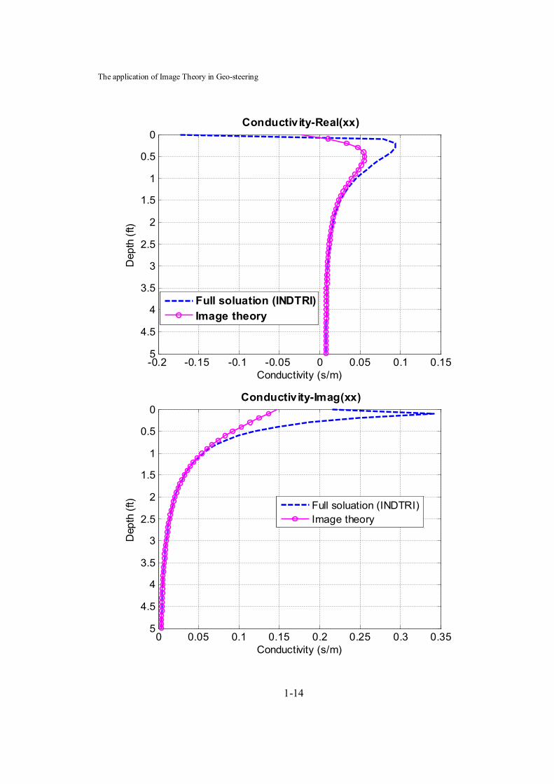
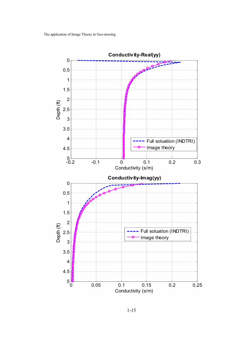
4.1 Two-layer model A two-layer model with the boundary at z = 0ft is shown in Figure 11. The parameter of
the two layers are 1 1 110, 1, 1 for the upper layer and 1 1 110, 1, 0.01 for
the lower layer respectively. Because the approximated image theory only works when

The application of Image Theory in Geo-steering
1-13
the transmitter is within the high resistivity layer, the simulation results will only be
compared in the region of the lower layer. The two-layer model will be tested using two
different tools.
Sig = 1s/m
Sig = 0.01s/m
Figure 11 Two-layer model
a) Tool 1:
Frequency = 2000000 Hz
Spacing = 17in
Transmitter:
Number = 1
Turn = 1
Receiver:
Number = 1
Turn = 1
Figure 12 shows the the tool response of different components. The simulation results
are compared with the full solution results. From the figures, we can see that in most
ranges, except when the tool is approaching the boundary, the complex image method
works very vell. The relative error is less than 10% when the tool is two feet away from
the boundary. Considering the application scenario, this algorithm may be useful for the
Geo-steering control, since the bit should be steered away before the the tool reaches two
feet from the boundary.
The application of Image Theory in Geo-steering
1-14
-0.2 -0.15 -0.1 -0.05 0 0.05 0.1 0.15
0
0.5
1
1.5
2
2.5
3
3.5
4
4.5
5
Conductivity (s/m)
Dep
th (f
t)Conductivity-Real(xx)
Full soluation (INDTRI)Image theory
0 0.05 0.1 0.15 0.2 0.25 0.3 0.35
0
0.5
1
1.5
2
2.5
3
3.5
4
4.5
5
Conductivity (s/m)
Dep
th (f
t)
Conductivity-Imag(xx)
Full soluation (INDTRI)Image theory
The application of Image Theory in Geo-steering
1-15
-0.2 -0.1 0 0.1 0.2 0.3
0
0.5
1
1.5
2
2.5
3
3.5
4
4.5
5
Conductivity (s/m)
Dep
th (f
t)Conductivity-Real(yy)
Full soluation (INDTRI)Image theory
0 0.05 0.1 0.15 0.2 0.25
0
0.5
1
1.5
2
2.5
3
3.5
4
4.5
5
Conductivity (s/m)
Dep
th (f
t)
Conductivity-Imag(yy)
Full soluation (INDTRI)Image theory

The application of Image Theory in Geo-steering
1-16
-0.1 0 0.1 0.2 0.3
0
0.5
1
1.5
2
2.5
3
3.5
4
4.5
5
Conductivity (s/m)
Dep
th (f
t)Conductivity-Real(zz)
Full soluation (INDTRI)Image theory
0 0.05 0.1 0.15 0.2 0.25 0.3 0.35
0
0.5
1
1.5
2
2.5
3
3.5
4
4.5
5
Conductivity (s/m)
Dep
th (f
t)
Conductivity-Imag(zz)
Full soluation (INDTRI)Image theory

The application of Image Theory in Geo-steering
1-17
-1 -0.8 -0.6 -0.4 -0.2 0
0
0.5
1
1.5
2
2.5
3
3.5
4
4.5
5
Conductivity (s/m)
Dep
th (f
t)Conductivity-Real(xz)
Full soluation (INDTRI)Image theory
-0.4 -0.3 -0.2 -0.1 0
0
0.5
1
1.5
2
2.5
3
3.5
4
4.5
5
Conductivity (s/m)
Dep
th (f
t)
Conductivity-Imag(xz)
Full soluation (INDTRI)Image theory

The application of Image Theory in Geo-steering
1-18
0 0.2 0.4 0.6 0.8 1
0
0.5
1
1.5
2
2.5
3
3.5
4
4.5
5
Conductivity (s/m)
Dep
th (f
t)
Conductivity-Real(zx)
Full soluation (INDTRI)Image theory
0 0.1 0.2 0.3 0.4
0
0.5
1
1.5
2
2.5
3
3.5
4
4.5
5
Conductivity (s/m)
Dep
th (f
t)
Conductivity-Imag(zx)
Full soluation (INDTRI)Image theory
Figure 12 xx, yy, zz, xz and zx components of tool response in 2MHz

The application of Image Theory in Geo-steering
1-19
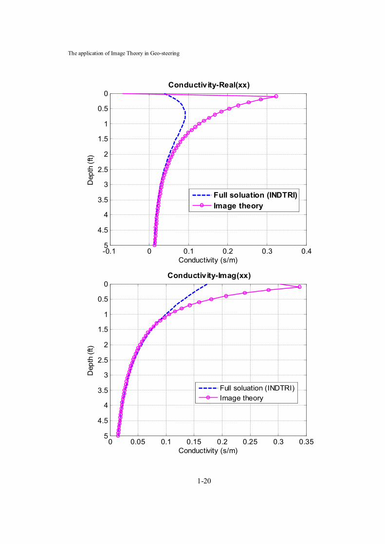
b) Tool 2
A two-layer model was also tested for a 400kHz tool with 34-inch spacing. Figure 13
shows the different components of tool response. Because the dipping angle is always
equal to 90o, the xz component and zx component are identical. Only the xx component,
yy component, zz component and xz component are shown. Compared with the 2MHz
tool, the image thoery has more error at the lower frequency, which is expected. This is
because when the frequency is lower, the skin depth of the conductor will be greater.
Then the error between the perfect conductor and the finite conductor will be larger. The
image approximation method has bigger errors.
The simulation results also show that, when the logging tool is working at 400kHz with
34 inch spacing, the relative accuracy range is within three feet away from the boundary,
which also could be considered as the effective application zone of Geo-steering,
compared to the physical dimension of tool and formation.
Frequency = 400000 Hz
Spacing = 34 in
Transmitter:
Number = 1
Turn = 1
Receiver:
Number = 1
Turn = 1
The application of Image Theory in Geo-steering
1-20
-0.1 0 0.1 0.2 0.3 0.4
0
0.5
1
1.5
2
2.5
3
3.5
4
4.5
5
Conductivity (s/m)
Dep
th (f
t)Conductivity-Real(xx)
Full soluation (INDTRI)Image theory
0 0.05 0.1 0.15 0.2 0.25 0.3 0.35
0
0.5
1
1.5
2
2.5
3
3.5
4
4.5
5
Conductivity (s/m)
Dep
th (f
t)
Conductivity-Imag(xx)
Full soluation (INDTRI)Image theory

The application of Image Theory in Geo-steering
1-21
-0.1 0 0.1 0.2 0.3
0
0.5
1
1.5
2
2.5
3
3.5
4
4.5
5
Conductivity (s/m)
Dep
th (f
t)Conductivity-Real(yy)
Full soluation (INDTRI)Image theory
0 0.05 0.1 0.15 0.2 0.25 0.3 0.35
0
0.5
1
1.5
2
2.5
3
3.5
4
4.5
5
Conductivity (s/m)
Dep
th (f
t)
Conductivity-Imag(yy)
Full soluation (INDTRI)Image theory

The application of Image Theory in Geo-steering
1-22
-0.1 0 0.1 0.2 0.3 0.4
0
0.5
1
1.5
2
2.5
3
3.5
4
4.5
5
Conductivity (s/m)
Dep
th (f
t)Conductivity-Real(zz)
Full soluation (INDTRI)Image theory
0 0.05 0.1 0.15 0.2 0.25 0.3 0.35
0
0.5
1
1.5
2
2.5
3
3.5
4
4.5
5
Conductivity (s/m)
Dep
th (f
t)
Conductivity-Imag(zz)
Full soluation (INDTRI)Image theory

The application of Image Theory in Geo-steering
1-23
-1 -0.8 -0.6 -0.4 -0.2 0 0.2 0.4
0
0.5
1
1.5
2
2.5
3
3.5
4
4.5
5
Conductivity (s/m)
Dep
th (f
t)Conductivity-Real(xz)
Full soluation (INDTRI)Image theory
-0.4 -0.3 -0.2 -0.1 0 0.1 0.2 0.3
0
0.5
1
1.5
2
2.5
3
3.5
4
4.5
5
Conductivity (s/m)
Dep
th (f
t)
Conductivity-Imag(xz)
Full soluation (INDTRI)Image theory
Figure 13 xx, yy, zz and xz components of tool response in 400KHz

The application of Image Theory in Geo-steering
1-24
4.2 Three-layer model The three-layer model with the boundary at z = -5ft and z = 5ft respectively is shown in
Figure 14. The parameter of the three layers are 1 1 110, 1, 1 for the upper layer,
1 10 , 1 11, 0.05 for the middle layer and 1 1 110, 1, 2 for the lower layer
respectively. Because the approximated image theory only works when the transmitter is
within the high resistivity layer, the simulation results will only be compared when the
tool is in the middle layer, -5< z <5. The three-layer model will be tested for two different
tools.
Sig = 1s/m
Sig = 0.05s/m
Sig = 2s/m
z = -5ft
z = 5ft z (ft)
Figure 14 Three-layer model
a) Tool 1:
Frequency = 2000000 Hz
Spacing = 17 in
Transmitter:
Number = 1
Turn = 1
Receiver:
Number = 1
Turn = 1

The application of Image Theory in Geo-steering
1-25
The simulation results of the three-layer model for the Tool 1 at 2MHz are shown in
Figure 15. From Figure 15, we can see that the results are similar to what was discussed
in the two-layer model. When the drilling bit is further away from the boundary more
than two feet, the approximated image method is rather accurate. Only when the bit is
approaching the boundary, almost one and a half feet away from the boundary, does the
error increase. Among all the tool responses, xx, yy and zz have a relatively large margin
of error. The xz component, the one with the boundary information and the one in which
we are more interested, agrees with the full solution almost from one foot away from the
boundary. Compared with the imaginary part, the real part of each component has a
higher accuracy. Then actually we can obtain a higher accuracy by post-processing the
measured results. The reason for this is that in the data processing of obtaining the phase
difference and attenuation, only the real part of each component is involved.
-0.6 -0.5 -0.4 -0.3 -0.2 -0.1 0 0.1
-5
-4
-3
-2
-1
0
1
2
3
4
5
Conductivity (s/m)
Dep
th (f
t)
Conductivity-Real(xx)
Full soluation (INDTRI)Image theory

The application of Image Theory in Geo-steering
1-26
0 0.05 0.1 0.15 0.2 0.25 0.3 0.35
-5
-4
-3
-2
-1
0
1
2
3
4
5
Conductivity (s/m)
Dep
th (f
t)Conductivity-Imag(xx)
Full soluation (INDTRI)Image theory
-0.2 -0.1 0 0.1 0.2 0.3 0.4 0.5
-5
-4
-3
-2
-1
0
1
2
3
4
5
Conductivity (s/m)
Dep
th (f
t)
Conductivity-Real(yy)
Full soluation (INDTRI)Image theory

The application of Image Theory in Geo-steering
1-27
0 0.05 0.1 0.15 0.2 0.25 0.3 0.35
-5
-4
-3
-2
-1
0
1
2
3
4
5
Conductivity (s/m)
Dep
th (f
t)Conductivity-Imag(yy)
Full soluation (INDTRI)Image theory
-0.4 -0.3 -0.2 -0.1 0 0.1 0.2 0.3
-5
-4
-3
-2
-1
0
1
2
3
4
5
Conductivity (s/m)
Dep
th (f
t)
Conductivity-Real(zz)
Full soluation (INDTRI)Image theory

The application of Image Theory in Geo-steering
1-28
-0.05 0 0.05 0.1 0.15 0.2 0.25 0.3
-5
-4
-3
-2
-1
0
1
2
3
4
5
Conductivity (s/m)
Dep
th (f
t)Conductivity-Imag(zz)
Full soluation (INDTRI)Image theory
-1 -0.5 0 0.5 1
-5
-4
-3
-2
-1
0
1
2
3
4
5
Conductivity (s/m)
Dep
th (f
t)
Conductivity-Real(xz)
Full soluation (INDTRI)Image theory

The application of Image Theory in Geo-steering
1-29
-1.5 -1 -0.5 0 0.5 1 1.5 2
-5
-4
-3
-2
-1
0
1
2
3
4
5
Conductivity (s/m)
Dep
th (f
t)Conductivity-Imag(xz)
Full soluation (INDTRI)Image theory
Figure 15 Three-layer model xx, yy, zz, xz and zx componets of tool response in 2MHz
b) Tool 2
Frequency = 400000 Hz
Spacing = 34 in
Transmitter:
Number = 1
Turn = 1
Receiver:
Number = 1
Turn = 1

The application of Image Theory in Geo-steering
1-30
-2 -1 0 1 2
-5
-4
-3
-2
-1
0
1
2
3
4
5
Conductivity (s/m)
Dep
th (f
t)Conductivity-Real(xz)
Full soluation (INDTRI)Image theory
-1.5 -1 -0.5 0 0.5 1 1.5
-5
-4
-3
-2
-1
0
1
2
3
4
5
Conductivity (s/m)
Dep
th (f
t)
Conductivity-Imag(xz)
Full soluation (INDTRI)Image theory
Figure 16 Three-layer model xz component of tool response in 400KHz

The application of Image Theory in Geo-steering
1-31
Figure 16 shows the xz component of the tool response at 400k in the three-layer model.
From the results we can see that, although at 400kHz the approximation method has less
accuracy, the result from the image theory and the result from the full solution still have
good agreement when the distance away from boundary is greater than three feet.
4.3 Tolerance In this section, the tolerance of the image method at different frequencies and
conductivities will be investigated in the two-layer model, as shown in Figure 11. The
upper layer of the model is the high conductivity layer, which will always be equal to
1m/s. The lower layer of the model is a low conductivity layer. The conductivity of the
formation is changed from 0.1m/s to 0.001m/s. The tolerance of the image method is
tested for two different tools, 2MHz and 400kHz, respectively. For each tool, at a specific
obeservation point, the absolute error and relative error will be given along with the
different conductivity ratio between the upper layer and lower layer.
a) Tool 1:
Frequency = 2000000 Hz
Spacing = 17 in
Transmitter:
Number = 1
Turn = 1
Receiver:
Number = 1
Turn = 1
Figure 17 and Figure 18 show the absolute error and relative error between the
approximation results and full solution results at the observation point one foot away
from the boundary. The results show that when the resistivity ratio between the upper
layer and the lower layer is increased, the error between the approximation method and

The application of Image Theory in Geo-steering
1-32
the full solution converges. The error of the xz component is smaller when the resistivity
ratio of the upper layer and the lower layer is larger. At the observation point one foot
away from the boundary, when the resistivity ratio between the upper layer and the lower
layer is ,more than 100, the absolute error is less than 0.0123; the relative error between
the approximation method and the full solution is about 15%.
Consider another receiver: two feet away from the boundary. Figure 19 and Figure 20
give the absolute error and relative error variation as a function of the resistivity ratio of
the upper layer and the lower layer. The results show that the tool gives more accurate
results when the tool is two feet away from the boundary. When the resistivity ratio
between the upper layer and the lower layer is higher than 100, the relative error between
the approximation method and the full solution is about 11%.
200 400 600 800 10000
1
2
3
4
5
6x 10
-3Oberservation point 1ft away from boundary
Resistivity ratio
Err
or
Real(xx)Real(yy)Rea(zz)

The application of Image Theory in Geo-steering
1-33
200 400 600 800 10000.012
0.0125
0.013
0.0135
0.014
0.0145
0.015Oberservation point 1ft away from boundary
Resistivity ratio
Err
or
Real(xz)
Figure 17 Absolute error of 2MHz tool at 1ft away from boundary
200 400 600 800 10000
2
4
6
8
10
12
14
16Oberservation point 1ft away from boundary
Resistivity ratio
Err
or(%
)
Real(xx)Real(yy)Rea(zz)

The application of Image Theory in Geo-steering
1-34
200 400 600 800 100014
16
18
20
22
24
26
28Oberservation point 1ft away from boundary
Resistivity ratio
Err
or(%
)
Real(xz)
Figure 18 Relative error of 2MHz tool at 1ft away from boundary
200 400 600 800 10000
0.2
0.4
0.6
0.8
1
1.2
1.4x 10
-3Oberservation point 2ft away from boundary
Resistivity ratio
Err
or
Real(xx)Real(yy)Rea(zz)

The application of Image Theory in Geo-steering
1-35
200 400 600 800 10001.44
1.46
1.48
1.5
1.52
1.54
1.56x 10
-3Oberservation point 2ft away from boundary
Resistivity ratio
Err
or
Real(xz)
Figure 19 Absolute error of 2MHz tool at two feet away from boundary
200 400 600 800 10000
1
2
3
4
5
6
7Oberservation point 2ft away from boundary
Resistivity ratio
Err
or(%
)
Real(xx)Real(yy)Rea(zz)

The application of Image Theory in Geo-steering
1-36
200 400 600 800 100010
15
20
25
30
35
40
45
50
55Oberservation point 2ft away from boundary
Resistivity ratio
Err
or(%
)
Real(xz)
Figure 20 Relative error of 2MHz tool at two feet away from boundary
b) Tool 2
Frequency = 400000 Hz
Spacing = 34 in
Transmitter:
Number = 1
Turn = 1
Receiver:
Number = 1
Turn = 1
The same testing is done for the 400KHz tool. Compared with the 2MHz tool, the
400KHz tool has less accuracy. The two observation points are chosen a little bit further
away from the boundary, two feet and three feet.

The application of Image Theory in Geo-steering
1-37
200 400 600 800 10000
1
2
3
4
5
6
7
8
9x 10
-3Oberservation point 2ft away from boundary
Resistivity ratio
Err
or
Real(xx)Real(yy)Rea(zz)
200 400 600 800 10000.0085
0.009
0.0095
0.01
0.0105
0.011
0.0115
0.012
0.0125
0.013Oberservation point 2ft away from boundary
Resistivity ratio
Err
or
Real(xz)
Figure 21 Absolute error of 400kHz tool at two feet away from boundary

The application of Image Theory in Geo-steering
1-38
200 400 600 800 10000
5
10
15
20
25Oberservation point 2ft away from boundary
Resistivity ratio
Err
or(%
)
Real(xx)Real(yy)Rea(zz)
200 400 600 800 100010
12
14
16
18
20
22Oberservation point 2ft away from boundary
Resistivity ratio
Err
or(%
)
Real(xz)
Figure 22 Relative error of 400kHz tool at two feet away from boundary

The application of Image Theory in Geo-steering
1-39
200 400 600 800 10000
0.5
1
1.5
2
2.5
3x 10
-3Oberservation point 3ft away from boundary
Resistivity ratio
Err
or
Real(xx)Real(yy)Rea(zz)
200 400 600 800 10003.6
3.8
4
4.2
4.4
4.6
4.8x 10
-3Oberservation point 3ft away from boundary
Resistivity ratio
Err
or
Real(xz)
Figure 23 Absolute error of 400kHz tool at three feet away from boundary

The application of Image Theory in Geo-steering
1-40
200 400 600 800 10000
2
4
6
8
10
12Oberservation point 3ft away from boundary
Resistivity ratio
Err
or(%
)
Real(xx)Real(yy)Rea(zz)
200 400 600 800 100010
12
14
16
18
20
22
24
26
28Oberservation point 3ft away from boundary
Resistivity ratio
Err
or(%
)
Real(xz)
Figure 24 Relative error of 400kHz tool at three feet away from boundary

The application of Image Theory in Geo-steering
1-41
4.4 Computation time Machine parameters: operation system: Window XP
processor: Intel @ 2.33GHz
Memory(RAM):8.00GB
Testing model: Three-layer model (Figure 14)
Testing tool: Frequency = 2MHz Spacing = 19
Z_start, Z_end, Z_step: -30, 30 , 0.1
Number of logging point: 600 (single routine)
Table 1: Computation time comparison
Iterative Times 10 100 1000
Image Method (s) 0.1201728 0.590845 5.367719
Full Solution (s) 8.672470 86.17391 859.8765
Speed Ratio 72.167 150.926 160.1940228
Table 1 shows the CPU time comparson between the image method and the full solution
for different numbers of iterations. The results show that the image method is much faster
than the full solution. When iteration time is 1000, the image method is 160 times faster
than the full solution. In addition, when iterative times increase, the image method will
have a greater advantage in computation speed.
5. Conclusion
Image theory, as a method used to simplfy the inhomogenous media to homogenous
media, can be applied in Geo-steering to speed up the simulation. The advantage of this
theory is to simplify calculation and to speed up simulation. The limitation is that the
complex image theory can be only used in the situation when the source is within the
high resistivity layer, compared with other boundary layers. However, this specific
requirement satisfies most G
eo-steering applications.

The application of Image Theory in Geo-steering
1-42
The image approximation method was tested at 2MHz and 400KHz respectively.
Compared with the full solution results, the complex image method has very good
agreement at both frequencies. The image method has signifiant error when the tool is
two feet and three feet away from the bed boundary. It works better at high frequencies.
This is because when the frequency is higher, the skin depth of the conductor is shorter,
which is closer to a perfect conductor,, and therefore the image theory is more accurate.
The accuracy of the complex image theory also depends on the conductivities of both
layers. When the error decreases, the conductivity difference between the upper layer and
the lower layer increases. The absolute error and relative error are collected at different
observation points. Closer to the boundary, the error is larger. For the 2MHz tool, when
the logging point away from the boundary is more than two feet, we can obtain a higher
accuracy. For the 400KHz tool, this distance is increased to three feet.
Compared with the full solution method, the image approximation method can
significantly speed up the simulation. For a 1000 iteration, 600 logging points in each
routine, the image method is 160 times faster than the full solution. This time difference
is also enlarged along with the increase of the logging point.

The application of Image Theory in Geo-steering
1-43
Reference
[1] M. Bittar, J. Klain, G. Hu, J. Pitcher, C. Golla, G. Althoff, M. Sitka, V. Minosyan
and M. Paulk, "A new azimuthal deep-reading resistivity tool for geo-steering and
advanced formation evaluation," SPE Annual Technical Conference and
Exhibition, SPE 109971, 2007.
[2] Q. Li, D. Omeragic, L. Chou, L. Yang, K. Duong, J. Smits, J. Yang, T. Lau, C.
Liu, R. Dworak, V. Dreuillault and H. Ye, "New directional electromagnetic tool
for proactive geo-steering and accurate formation evaluation while drilling," 46th
SPWLA Annual Logging Symposium, Paper UU, 2005.
[3] T. Wang, H. Meyer and L. Yu, "Dipping bed response and inversion for distance
to bed for a new while-drilling resistivity measurement," SEG New Orleans 2006
Annual Meeting, pp. 416-420, 2006.
[4] J. R. Wait, "Image theory of a quasi-static magnetic dipole over a dissipative
half-space," Electron. Letter. Vol. 5, No. 13, pp. 281-282, June, 1969.
[6] I. V. Lindell and E. Alanen, "Exact image theory for the Sommerfeld half-space
problem, Part I: Vertical magnetic dipole," IEEE Trans. Antennas Propagateion,
Vol. AP-32, No. 2, pp. 126-133, February, 1984.
[5] P. R. Bannister, "Summary of image field expressions for the quasi-static fields of
antennas at or above the earth's surface," Proceedings of the IEEE, Vol. 67,No. 7,
July, 1979.
[7] T. Wang and Q. Z. Dong, "A fast forward model for simulating a layered medium
using the complex image theory," SEG San Antonio 2011Annual Meeting, pp.
573-577, 2011.
[8] D. Omeragic, T. Habashy, C. Esmersoy, Q. Li, J. Seydoux, J. Smits and J. R.
Tabanou, "Real-time interpretation of formation structure from directional EM
measurements," SPWLA 47th Annual Logging Symposium, June 4-7, 2006.

Preliminary Study of Look-Ahead Resistivity Logging Tools
2-1
CHAPTER 2
Preliminary Study of Look-Ahead Resistivity Logging Tools
Abstract
Look-ahead measurement is to detect the formation properties ahead of the drill bit. In
geosteering operations, accurate controlling of drilling trajectory often benefits from the
prediction of the target-formation properties. Using resistivity logging tools, we can
detect an anomaly ahead of the drill bit, such as a problem zone or a boundary. However,
conventional logging tools with coil antennas are not designed for look-ahead purposes,
and hence may not be optimal when used in such scenarios. In this paper, we modeled the
resistivity logging tool with several different types of sources, and investigated the
electromagnetic fields they generate in front of the drill bit. By comparing the attenuation
of the normalized fields simulated under various conditions, we were able to assess the
look-ahead capability of each type of source, and to determine the optimized excitation
form for a new look-ahead tool design.
1. Introduction
The past two decades have seen dramatically increasing demands in horizontal drilling.
In order to achieve the most cost-effective production, wells can be designed with very
complicated trajectories. In modern geosteering operations, directional drillers mainly
refer to the formation model that is built beforehand based on seismic interpretation, log
analysis and geological mapping [1]. However, the formation modeling inevitably
involves estimation and interpolation, which result in uncertainties between modeled
strata and the real formation structures the bit will pass. To guide the bit towards the
target layers, operators need to monitor the well logs in real time, especially the data that
suggest formation variations ahead of the drill bit.

Preliminary Study of Look-Ahead Resistivity Logging Tools
2-2
Look-ahead logging is to take measurements of, or to look axially into the formations
before they are encountered by the bit. Using look-ahead logs, one can detect the
existence of an anomaly in advance. Such anomalies can be an over-pressured shale zone,
which may cause serious troubles when drilled through without adequate preparation [2].
Once the well enters the target area, the driller’s objective is to keep the well path within
the pay zone, avoiding the unproductive layers and/or boundaries. As a result, the
accuracy of drilling is greatly affected by the look-ahead capability of the logging tools.
Resistivity logging tools make measurements by emitting radio-frequency waves and
generate electromagnetic fields in the formations. The receiver response is closely related
to the formation conductivity, and thus an indication of lithology or the presence of
hydrocarbon reservoir. Conventional resistivity logging tools use coils as transmitter and
receiver antennas, and generally sees several feet laterally into the formations. [2] and [3]
discussed the look-ahead potentials of coil antenna with no mandrels, using both time-
domain and frequency-domain methods. However, induction logging tool with coils was
not specially designed for look-ahead purposes, so it may be not optimal when applied
under such conditions. To develop a look-ahead logging tool, we need to first determine
an optimized source, or an appropriate form of electromagnetic excitation, which can
provide better performance in predicting the formation resistivity ahead of the bit.
Fig. 1 Tool configuration Fig. 2 Induction logging tool with coil antenna

Preliminary Study of Look-Ahead Resistivity Logging Tools
2-3
In this paper, we modeled the tool with four types of sources: coil, gap, dipole, and
surface current along the mandrel. By investigating the ahead-of-the-bit fields generated
by each source, we discussed the tool behaviors in response to the conductivity variation
respectively, and then compared the field attenuation with respect to distance from the
drill bit. Conclusions and suggested future work are presented at the end.
2. Frequency-Domain Tool Modeling
The prototype tool used in simulations is captured in Fig. 1. The tool consists of a source,
or a transmitter antenna, and a finite-size metal mandrel. An infinite homogeneous
formation is assumed, with a conductivity of f that varies from 0.1-10 S/m. The field of
interest is ahead of the drill bit, so no receiver is involved here. L represents the distance
from source to bit. For each type of source, two values of L are used: 0.8 m and 10 m,
indicating the tool is near bit or not. Corresponding fields are investigated in each
scenario, with the observation point moving axially away from the drill bit. The operation
frequency is 10 kHz.
2.1 Coil antenna
Coils, excited by an alternating current, are used in induction logging as transmitter and
receiver antennas. As illustrated in Fig. 2, the magnetic fields produced by the transmitter
induce eddy currents in the formation surrounding the wellbore, the intensity of which is
approximately proportional to the conductivity [4]. When the coil area is much smaller
than wavelength, it can be modeled as a vertical magnetic dipole.
Using a single-turn coil antenna wound on a conductive mandrel to calculate the
azimuthal current density J with finite element method, we get the results shown in Fig.
3.

Preliminary Study of Look-Ahead Resistivity Logging Tools
2-4
(a)
(b)
Fig. 3 Current density ahead of the drill bit, coil antenna. (a) L = 0.8 m; (b) L = 10 m.

Preliminary Study of Look-Ahead Resistivity Logging Tools
2-5
Fig. 4 Current density affected by conductivity, coil antenna, d = 0.5 m.
When the transmitter is near the drill bit (L = 0.8 m), J increases with the formation
conductivity, forming a linear relationship shown in Fig. 4. However, if the transmitter
coil is far above the bit (L = 10 m), the relationship between J and f is no longer
monotonous. This phenomenon results from the skin depth effect caused by the
increasing of conductivity. In principle, the inductive current intensity benefits from the
conductivity, but over a long distance from the source to bit, the field attenuation is not
negligible. After f grows beyond 1 S/m, the skin depth effect eventually dominates the
overall result.
Fig. 5 Voltage-gap source and current-gap source
0 2 4 6 8 10
|Jφ| (
A/m
2 )
Formation conductivity (S/m)
L = 0.8 mL = 10 m

Preliminary Study of Look-Ahead Resistivity Logging Tools
2-6
(a)
(b)
Fig. 6 Electric field ahead of the bit, voltage-gap source. (a) L = 0.8 m; (b) L = 10 m.

Preliminary Study of Look-Ahead Resistivity Logging Tools
2-7
2.2 Gap source
Another excitation method in practical use is gap source. The drill string is cut into two
parts, and separated with an electric insulator. An alternating voltage or current is applied
within the insulator, to produce currents along the drill string and then through the
formation, as shown in Fig. 5.
Here we modeled with both voltage and current sources. The results are given in Fig. 6 -
Fig. 8. The figures show that the behavior of gap source is quite different from coil
antennas. In both 0.8-m and 10-m cases, the vertical electric field decreases exponentially
as the conductivity grows up. That means, when the formation turns conductive, the
currents become more concentrated around the source, and in turn contribute less to the
ahead-of-the-bit field.
The results in Fig. 8 also demonstrated that no matter the gap is near bit or otherwise, the
performance of voltage-gap is almost identical with current-gap.
(a)

Preliminary Study of Look-Ahead Resistivity Logging Tools
2-8
(b)
Fig. 7 Electric field ahead of the bit, current-gap source. (a) L = 0.8 m; (b) L = 10 m.
(a) (b)
Fig. 8 Electric field affected by conductivity, gap source.
(a) L = 0.8 m, d = 0.5 m; (b) L = 10 m, d = 2.5 m.
0
10
20
30
40
50
60
0
0.05
0.1
0.15
0.2
0.25
0 5 10
Elec
tric
field
|Ez
| (V
/m)
Formation conductivity (S/m)
voltage sourcecurrent source
0
0.5
1
1.5
2
2.5
00.05
0.10.15
0.20.25
0.30.35
0.40.45
0.5
0 5 10
Elec
tric
field
|Ez
| (V
/m)
Formation conductivity (S/m)
voltage sourcecurrent source

Preliminary Study of Look-Ahead Resistivity Logging Tools
2-9
2.3 Horizontal Electric Dipole
An electric dipole is a pair of separated electric charges, with equal magnitude and
opposite signs, while a magnetic dipole is a small current loop. In practice, a toroidal
antenna with wires wound on a magnetic torus can be seen as an electric dipole.
Fig. 9 Dipole sources
(a)

Preliminary Study of Look-Ahead Resistivity Logging Tools
2-10
(b)
Fig. 10 Electric field ahead of the bit, electric dipole. (a) L = 0.8 m; (b) L = 10 m.
(a)

Preliminary Study of Look-Ahead Resistivity Logging Tools
2-11
(b)
Fig. 11 Current density ahead of the bit, magnetic dipole. (a) L = 0.8 m; (b) L = 10 m.
(a) (b)
Fig. 12 Electric field affected by conductivity, dipole source.
(a) Electric dipole; (b) Magnetic dipole.
0 2 4 6 8 10
|Ey|
(V/m
)
Formation conductivity (S/m)
L = 0.8 m, d = 0.5 m
L = 10 m, d = 2.5 m
0
0.5
1
1.5
2
2.5
0
5
10
15
20
25
0 5 10
|Jz|
(A/m
2 )
Formation conductivity (S/m)
L = 0.8 m, d = 0.5 m
L = 10 m, d = 2.5 m

Preliminary Study of Look-Ahead Resistivity Logging Tools
2-12
Here we investigated the fields of both electric and magnetic dipoles with the existence of
a conductive mandrel. The dipole is perpendicular to the tool axis, as shown in Fig. 9.
The results are given in Fig. 10 - Fig. 12. For electric dipole, the results are similar with
that of gap excitation in the way that the look-ahead capability is affected by the
formation conductivity. Magnetic dipole produces inductive fields like coils, so the skin
depth effect appears in the 10-m case as well when f > 1 S/m.
2.4 Surface current
In this model, we applied a surface current along the mandrel. Results are shown in Fig.
13 and Fig. 14. Since the current is constant along the tool axis, the distance from source
to bit is zero. For comparison, we built mandrels of different lengths, as used in previous
models. In general, the fields get intensified as the conductivity increases. When a short
mandrel is used, the current density is proportional to the conductivity as coil antenna
does. For a long mandrel, the relationship between J and f is no longer linear. The
skin depth effect becomes stronger as the observation point moves away from the drill bit.
3. Comparison
To compare between different source models, the normalized fields from each model are
plotted in Fig. 15. In both mandrel configurations, coil antenna and horizontal electric
dipole showed better performance than any others. Both of them have an axial component
of magnetic field, which is enhanced by the metal mandrel, and in turn produces stronger
electric field or current ahead of the bit. In the near-bit case, the attenuation of coil and
electric dipole is about two times lower than others; while for longer L, the advantage is
even more significant. This result suggests that other than coil antenna, horizontal electric
dipole or toroidal antenna also has potentials to look deep into the formation with the
existence of the mandrel.

Preliminary Study of Look-Ahead Resistivity Logging Tools
2-13
(a)
(b)
Fig. 13 Current density ahead of the bit, surface current. (a) short mandrel; (b) long mandrel.

Preliminary Study of Look-Ahead Resistivity Logging Tools
2-14
Fig. 14 Current density affected by conductivity, surface current 4 Conclusions
Four types of source are modeled for a look-ahead resistivity logging tool. Simulations
are conducted under various conditions to evaluate the look-ahead capability of each
source model. The results have shown that other than the commonly-used coil induction
logging tools, a horizontal electric dipole, or a toroidal antenna can also be considered as
an alternative of the transmitter.
To further investigate the look-ahead capability of the logging tools, a simple
homogeneous formation model would not be adequate. More aspects of the formation
parameters, such as multi-layers and dipping angle, will be involved in the future
research.
0
0.05
0.1
0.15
0.2
0.25
0.3
0
0.005
0.01
0.015
0.02
0.025
0.03
0.035
0.04
0 2 4 6 8 10
|J z|
(A/m
2 )
Formation conductivity (S/m)
Short, d = 0.5 m
Short, d = 1.0 m
Long, d = 0.5 m
Long, d = 1.0 m
Long, d = 2.5 m

Preliminary Study of Look-Ahead Resistivity Logging Tools
2-15
(a)
(b)
Fig. 15 Comparison of fields ahead of the bit. (a) Short mandrel; (b) Long mandrel.
0
0.1
0.2
0.3
0.4
0.5
0.6
0.7
0.8
0.9
1
0 0.5 1 1.5 2
Nor
mal
ized
fiel
d
Distance from bit (m)
coil
gap_voltage
gap_current
E-dipole
H-dipole
surface current
0
0.1
0.2
0.3
0.4
0.5
0.6
0.7
0.8
0.9
1
0 5 10 15 20
Nor
mal
ized
fiel
d
Distance from bit (m)
coil
gap_voltage
gap_current
E-dipole
H-dipole
surface current

Preliminary Study of Look-Ahead Resistivity Logging Tools
2-16
Reference
[1] P. Hook, Predicting the path ahead, Middle East & Asia Reservoir Review, vol. 21,
1998, pp. 26-33.
[2] Q. Zhou, D. Gregory, S. Chen and W. C. Chew, Investigation on electromagnetic
measurement ahead of drill-bit, Geoscience and remote sensing symposium, 2000,
vol. 4, pp. 1745-1747.
[3] E. Banning, T. Hagiwara and R. Ostermeier, System and method for locating an
anomaly ahead of a drill bit, US patent 7538555, 2004.
[4] J. H. Moran and K. S. Kunz, Basic theory of induction logging and application to
study of two-coil sondes, Geophysics, vol. 27, no. 6, part 1, 1962, pp. 829-858.

Analysis of Pulsed Look Ahead Tools Using FDTD Method
3-1
CHAPTER 3
Analysis of Pulsed Look Ahead Tools Using FDTD Method
Abstract
Finite difference time domain method (FDTD) is one of most powerful numerical
solution to EM time domain problems especially in microwave frequencies. However,
in some areas, ultra low frequency (ULF) is required such as look ahead tools, and
sea-bed logging, EM problems in marine-subsurface, which means extremely large
number of time steps to get satisfied results. Thus, how to significantly reduce the
large time-steps becomes very important in such FDTD applications in ULF problems.
Here this paper proposed a new way to significantly reduce the total simulation time.
A 3D problem has been raised to be set as an example showing that the results are
satisfied with much smaller number of simulation time steps. The developed 3D
method is applied to solve the pulsed look-ahead tool response for detection of bed
boundaries in the time domain. Both frequency effects and formation detection
capabilities are investigated.
1. Introduction
Finite-difference (FD) method has already been widely used in many areas nowadays.
Those areas are not only engineering, science, technologies but even business,
economics. In this report, it mainly deals with the electromagnetic problems in look
ahead logging tools using one of the FD methods in the time domain.
The FD method is a method which is used to solve partial differential equations
numerically. The finite-difference time domain method was introduced by Yee in
1966. This method is mainly focusing on solving Maxwell’s equations. And it is very
successful and already been applied to many electromagnetic problems.

Analysis of Pulsed Look Ahead Tools Using FDTD Method
3-2
During the FDTD calculation, the speed of the calculation is very important for
engineers and problem solving. There are a lot of ways which increase the speed of
the FDTD algorithm such as Perfect Matched Layers (PML), up scaling of artificially
high electric permittivity. Both of those two has been implemented in the FDTD
algorithm in this report. 2. Background of Look-Ahead tool simulation 2.1. Introduction of look-ahead tool Look-ahead tool can be implemented in the time domain. The purpose of the look
ahead tool is to find the boundaries ahead of the drilling string. This kind of tools is
usually installed near the drill bits if possible. However, due to the limited space near
the bit, the tool sometimes has to be installed after the mud motor or rotary steerable
units as shown in Figure 1.
Figure 1. A schematic of a boundary detection look ahead tool
One of the implementation is to use an air gap as an excitation. The air gap can be
either a real insulation gap between two conducting electrode on the mandrel, or can
be a toroidal coil. In this study, we use air gap as excitation. The excitation consists
of 3 parts which are 2 PECs and 1 air gap portion. The tool configuration is shown in
Look ahead tool
Bed boundary

Analysis of Pulsed Look Ahead Tools Using FDTD Method
3-3
Figure 1. Two PECs are connected by the air part. The transmitter is actually a voltage
source centering inside the air gap. 2 receivers are located along the PEC pipe.
2.2. Voltage source simulation using finite difference time domain method
2.2.1. FDTD updating equations for lumped elements
Many practical electromagnetics applications require inclusion of lumped circuit
elements. The lumped elements may be active sources in the form of voltage and
current sources or passive in the form of resistors, inductors, and capacitors.
Nonlinear circuit elements such as diodes and transistors are also required to be
integrated in the numerical simulation of antennas and microwave devices. The
electric current flowing through theses circuit elements can be represented by the
impressed current density term, 퐽⃗ in Maxwell’s curl equation.
ei
EH E Jt
(1)
Impressed currents are used to represent sources or known quantities. In this sense,
they are the sources that cause the electric and magnetic fields in the computational
domain. A lumped element component placed between two nodes is characterized by
the relationship between the voltage V across and the current I flowing between these
two nodes. This relationship can be incorporated into the Maxwell’s curl equation (4.1)
by expressing 퐸⃗ in terms of V using
E V
(2)
And by expressing 퐽⃗ in terms of I using the relation
Figure 2. Look ahead tool structure, an air gap on the mandril is used to simulate the excitation
V

Analysis of Pulsed Look Ahead Tools Using FDTD Method
3-4
퐼 = ∫ 횥⃑ . 푑푠⃑ (3)
Where S is the cross-sectional area of a unit cell normal to the flow of the current I.
these equations can be implemented in discrete time and space and can be
incorporated into (4.1), which are expressed in terms of finite differences. Then, the
finite-difference time-domain (FDTD) updating equations can be obtained that
simulates the respective lumped element characteristics.
In this chapter we discuss the construction of the FDTD updating equations for
lumped element components.
Voltage source
In any electromagnetics simulation, one of the necessary components is the inclusion
of sources. Types of sources vary depending on the problem types; scattering
problems require incident fields from far zone sources, such as plane waves, to excite
objects in a problem space, whereas many other problems require near zone sources,
which are usually in the forms of voltage or current sources. In this section we derive
updating equations that simulate the effects of a voltage source present in the problem
space.
Consider the scalar curl equation below:
1 ( ).y exzz z iz
z
H HE E Jt x y
(4)
This equation constitutes the relation between the current density 퐽 ⃗ flowing in the z
direction and the electric and magnetic field vector components. Application of the
central difference formula to the time and space derivatives based on the field
positioning scheme.

Analysis of Pulsed Look Ahead Tools Using FDTD Method
3-5
11 ( , , ) ( 1, , )( , , ) ( , , ) 1( , , )
n nn ny yz z
z
H i j k H i j kE i j k E i j kt i j k x
1/2 1/2( , , ) ( , 1, )1( , , )
n nx x
z
H i j k H i j ki j k y
1( , , ) ( ( , , ) ( , , ))2 ( , , )
en nzz z
z
i j k E i j k E i j ki j k
1/21 ( , , ).( , , )
niz
z
J i j ki j k
(5)
We want to place a voltage source with sV volts magnitude and sR ohms internal
resistance between nodes ( , , )i j k and ( , , 1)i j k , where sV a time-varying function
with a predetermined waveform. The voltage-current relation for this circuit can be written as
,ss
V VIR
(6)
Where V is the potential difference between nodes ( , , )i j k and ( , , 1)i j k . The
term V can be expressed in terms of zE using (2), which translates to
1 11/2 ( , , ) ( , , )( , , ) ,
2
n nn z zz
E i j k E i j kV z E i j k z
(7)
In discrete form at time instant ( 0.5)n t . Current I is the current flowing
through the surface enclosed by the magnetic field components, which can be
expressed in terms of izJ using (3) as
1/2 1/2 ( , , ).n nizI x yJ i j k (8)
One should notice that V in (7) is evaluated at time instant ( 0.5)n t , which
corresponds to the required time instant of I and J dictated by (5). Inserting (7) and (8) in (6) one can obtain

Analysis of Pulsed Look Ahead Tools Using FDTD Method
3-6
1/2 1/2 1 1/21( ( , , ) ( , , )) .2
n n n niz z z s
s s
zJ E i j k E i j k Vx yR x yR
(9)
Equation (9) includes the voltage-current relation for a voltage source tying sV and
sR to electric field components in the discrete space and time. One can use (9) in (5)
and rearrange the terms such that the future values of the electric field component 1n
zE can be calculated using other terms, which yields our standard form updating
equations such that
1( , , ) ( , , ) ( , , )n nz eze zE i j k C i j k E i j k
1/2 1/2( , , ) ( ( , , ) ( 1, , ))n nezby y yC i j k H i j k H i j k
1/2 1/2( , , ) ( ( , , ) ( , 1, ))n nezbx x xC i j k H i j k H i j k
1/2( , , ) ( , , ),nezs sC i j k V i j k (10)
Where
2 ( , , ) ( , , )( , , )
2 ( , , ) ( , , )
2( , , )(2 ( , , ) ( , , ) )
2( , , )(2 ( , , ) ( , , ) )
( , , )
ez z
seze
ez z
s
ezbye
z zs
ezbxe
y ys
ezs
t zi j k t i j kx yRC i j k t zi j k t i j kx yR
tC i j k t zi j k t i j k xx yR
tC i j k t zi j k t i j k xx yR
C i j k
2 .(2 ( , , ) ( , , ) )( )e
y y ss
tt zi j k t i j k x yRx yR
Equation (10) is the FDTD updating equation modeling a voltage source placed
between the nodes ( , , )i j k and ( , , 1)i j k , which is oriented in the z direction. The
FDTD updating equations for voltage sources oriented in other directions can easily

Analysis of Pulsed Look Ahead Tools Using FDTD Method
3-7
be obtained following the same steps as just illustrated.
The FDTD updating equation (10) is given for a voltage source with a polarity in the
positive z direction. To model a voltage source with the opposite polarity, one needs
only to use the inverse of the voltage magnitude waveform by changing sV to sV .
2.2.2 Hard Voltage source In some applications it may be desired that a voltage difference is enforced between
two points in the problem space. This can be achieved by using a voltage source
without any internal resistances, which is called a hard voltage source. Voltage source
with sV volts magnitude is placed between the nodes ( , , )i j k and ( , , 1)i j k . The
FDTD updating equation for this voltage source can simply be obtained by letting
0sR in (10), which can be written as
1( , , ) ( , , ) ( , , )n nz eze zE i j k C i j k E i j k
1/2 1/2( , , ) ( ( , , ) ( 1, , ))n n
ezby y yC i j k H i j k H i j k
1/2 1/2( , , ) ( ( , , ) ( , 1, ))n n
ezbx x xC i j k H i j k H i j k (11)
1/2( , , ) ( , , ),n
ezs sC i j k V i j k Where:
( , , ) 1,( , , ) 0,
( , , ) 0,2( , , ) .
eze
ezby
ezbx
ezs
C i j kC i j k
C i j k
C i j kz
3. Numerical Results
3.1 Example 1
A 3 dimensional formation with a vertical boundary placed ahead of the tool. The
maximum frequency of the source is 1MHz differentiated gaussian wave as shown in

Analysis of Pulsed Look Ahead Tools Using FDTD Method
3-8
Figure 3. The purpose of this example is to investigate the tool response when the
frequency is high.
0 1 2 3 4 5 6 7 8
x 10-4
-8
-6
-4
-2
0
2
4
6x 10⁻³ Ex in homogenous case
Time(s)
Ex(
v)
Figure 3. A FDTD model of a look ahead tool near a low resistivity formation used to test the algorithm
Figure 4. Tool response in the time domain at the receiver when the formation is homogeneous, Ex component. The excitation pulse width is 1S.

Analysis of Pulsed Look Ahead Tools Using FDTD Method
3-9
0 1 2 3 4 5 6 7 8
x 10-4
-4
-3
-2
-1
0
1
2
3x 10⁻³ Ey in homogenous case
Time(s)
Ey(
v)
0 1 2 3 4 5 6 7 8
x 10-4
-0.15
-0.1
-0.05
0
0.05
0.1Ez in homogenous case
Time(s)
Ez(
v)
Figure 5. Tool response in the time domain at the receiver when the formation is homogeneous, Ey component. The excitation pulse width is 1S.
Figure 6. Tool response in the time domain at the receiver when the formation is homogeneous, Ez component. The excitation pulse width is 1S.

Analysis of Pulsed Look Ahead Tools Using FDTD Method
3-10
Figure 4, Figure 5, and Figure 6 show the computed results of the FDTD modeling
when the formation is homogeneous in which the conductive formation boundary is
removed. In the simulation, a 1 S width differential Gaussian pulse is used as the
source. The purpose of this modeling is to verify that the absorbing boundary
condition in the simulation is correctly placed so that the reflection wave is minimized
from the artificial boundaries. Figure 4 is the Ex component, Figure 5 and 6 are Ey
and Ez components at the receiver location.
Figure 7, Figure 8, and Figure 9 show the computed results of the FDTD modeling
when the formation is inhomogeneous in which the conductive formation boundary is
placed as shown in Figure 3. Figure 7 is the Ex component, Figure 8 and 9 are Ey and
Ez components at the receiver location. In each plot, the boundaries are placed at
three different locations: 6.56, 8.2, and 9.84 feet ahead of the drill bit. It is clearly
seen that the reflected waveforms changes as the distance of the boundary from the
drill bits changes.
0 1 2 3 4 5 6 7 8
x 10-6
-8
-6
-4
-2
0
2
4
6x 10⁻³
Time(s)
Ex(
v)
Ex vs Distance at Receiver 2
6.56 feet8.20 feet9.84 feet

Analysis of Pulsed Look Ahead Tools Using FDTD Method
3-11
Figure 7. Tool response in the time domain at the receiver when the formation is inhomogeneous, Ex component. The distance ahead of the drill bit is 6.56, 8.2, and 9.84 feet. The excitation pulse width is 1S.
Figure 8. Tool response in the time domain at the receiver when the formation is inhomogeneous, Ey component. The distance ahead of the drill bit is 6.56, 8.2, and 9.84 feet. The excitation pulse width is 1S.
0 1 2 3 4 5 6 7 8
x 10-6
-4
-3
-2
-1
0
1
2
3x 10⁻³
Time(s)
Ey(
v)Ey vs Distance at Receiver 2
6.56 feet8.20 feet9.84 feet
0 1 2 3 4 5 6 7 8
x 10-6
-0.15
-0.1
-0.05
0
0.05
0.1
Time(s)
Ez(
v)
Ez vs Distance at Receiver 2
6.56 feet8.20 feet9.84 feet

Analysis of Pulsed Look Ahead Tools Using FDTD Method
3-12
Figure 9. Tool response in the time domain at the receiver when the formation is inhomogeneous, Ez component. The distance ahead of the drill bit is 6.56, 8.2, and 9.84 feet. The excitation pulse width is 1S. Figure 7, Figure 8, and Figure 9 show the computed results of the FDTD modeling
when the formation is inhomogeneous in which the conductive formation boundary is
placed as shown in Figure 3. Figure 7 is the Ex component, Figure 8 and 9 are Ey and
Ez components at the receiver location. In each plot, the boundaries are placed at
three different locations: 6.56, 8.2, and 9.84 feet ahead of the drill bit. It is clearly
seen that the reflected waveforms changes as the distance of the boundary from the
drill bits changes.
Figure 10a, Figure 11a, and Figure 12a show the case of Figures 7, 8, and 9 when the
direct wave is subtracted from the total wave. Therefore, only reflected signals are left.
Figures 10b, 11b, and 12b are log-log plots of the corresponding waveform. From
these figures, we can see that the reflection signal amplitudes reduce with the distance
to boundary and time delay increases with the increase of the distance to boundary.
0 1 2 3 4 5 6 7 8
x 10-6
-8
-6
-4
-2
0
2
4
6
8
10x 10-4
Time(s)
Ex(
v)
Ex Secondary Wave vs Distance at Receiver 2
6.56 feet8.20 feet9.84 feet

Analysis of Pulsed Look Ahead Tools Using FDTD Method
3-13
Figure 10a. The reflection waveform after the direct wave is subtracted from the total waveform shown in Figure 7. Ex component. The distance ahead of the drill bit is 6.56, 8.2, and 9.84 feet. The excitation pulse width is 1S.
Figure 10b. Log plot of the reflection waveform after the direct wave is subtracted from the total waveform shown in Figure 7. Ex component. The distance ahead of the drill bit is 6.56, 8.2, and 9.84 feet. The excitation pulse width is 1S.
0 1 2 3 4 5 6 7 8
x 10-6
10-25
10-20
10-15
10-10
10-5
100
Time(s)
Ex(
v)
Ex Secondary Wave vs Distance at Receiver 2 in log scale
6.56 feet8.20 feet9.84 feet

Analysis of Pulsed Look Ahead Tools Using FDTD Method
3-14
Figure 11a. The reflection waveform after the direct wave is subtracted from the total waveform shown in Figure 8. Ey component. The distance ahead of the drill bit is 6.56, 8.2, and 9.84 feet. The excitation pulse width is 1S.
Figure 11b. The log plot of the reflection waveform after the direct wave is subtracted from the total waveform shown in Figure 8. Ey component. The distance ahead of the drill bit is 6.56, 8.2, and 9.84 feet. The excitation pulse width is 1S.
0 1 2 3 4 5 6 7 8
x 10-6
-6
-5
-4
-3
-2
-1
0
1
2
3
4x 10
-4
Time(s)
Ey(
v)
Ey Secondary Wave vs Distance at Receiver 2
6.56 feet8.20 feet9.84 feet
0 1 2 3 4 5 6 7
x 10-6
10-25
10-20
10-15
10-10
10-5
100
Time(s)
Ey(
v)
Ey Secondary Wave vs Distance at Receiver 2 in log scale
6.56 feet8.20 feet9.84 feet

Analysis of Pulsed Look Ahead Tools Using FDTD Method
3-15
Figure 12a. The reflection waveform after the direct wave is subtracted from the total waveform shown in Figure 9. Ez component. The distance ahead of the drill bit is 6.56, 8.2, and 9.84 feet. The excitation pulse width is 1S.
0 1 2 3 4 5 6 7 8
x 10-6
-0.015
-0.01
-0.005
0
0.005
0.01
0.015
0.02
Time(s)
Ez(
v)
Ez Secondary Wave vs Distance at Receiver 2
6.56 feet8.20 feet9.84 feet
0 1 2 3 4 5 6 7 8
x 10-6
10-20
10-15
10-10
10-5
100
Time(s)
Ez(
v)
Ez Secondary Wave vs Distance at Receiver 2 in log scale
6.56 feet8.20 feet9.84 feet

Analysis of Pulsed Look Ahead Tools Using FDTD Method
3-16
Figure 12b. The log plot of the reflection waveform after the direct wave is subtracted from the total waveform shown in Figure 9. Ey component. The distance ahead of the drill bit is 6.56, 8.2, and 9.84 feet. The excitation pulse width is 1S.
3.2. Example 2
A 3 dimensional formation with a vertical boundary placed ahead of the tool. The
maximum frequency of the source is 5kHz differentiated Gaussian wave. The same
formation is used in example 1. The purpose of this example is to investigate the tool
response when the frequency is low.
Figures 13, 14 and 15 are the received waveforms computed when the formation
boundary is removed for Ex, Ey and Ez components, respectively.
Figure 13. Tool response in the time domain at the receiver when the formation is homogeneous, Ex component. The excitation pulse width is 0.2mS.
0 0.2 0.4 0.6 0.8 1 1.2 1.4 1.6
x 10-3
-2
-1.5
-1
-0.5
0
0.5
1
1.5
2x 10⁻⁵ Ex in homogenous case
Time(s)
Ex(
v)

Analysis of Pulsed Look Ahead Tools Using FDTD Method
3-17
Figure 14. Tool response in the time domain at the receiver when the formation is homogeneous, Ey component. The excitation pulse width is 0.2mS.
Figure 15. Tool response in the time domain at the receiver when the formation is
0 0.2 0.4 0.6 0.8 1 1.2 1.4 1.6
x 10-3
-2
-1.5
-1
-0.5
0
0.5
1
1.5
2
2.5
3x 10
-5 Ey in homogenous case
Time(s)
Ey(
v)
0 0.2 0.4 0.6 0.8 1 1.2 1.4 1.6
x 10-3
-4
-3
-2
-1
0
1
2
3
4x 10⁻⁴ Ez in homogenous case
Time(s)
Ez(
v)

Analysis of Pulsed Look Ahead Tools Using FDTD Method
3-18
homogeneous, Ez component. The excitation pulse width is 0.2mS.
Figures 16, 17, and 18 are plots when the bed boundaries ahead of the drill bit is
placed at the distance of 66, 98, and 130 feet, respectively. It is seen that at low
frequencies the tool can “see” further.
Figures 16. Time domain response of the tool when the bed boundaries ahead of the drill bit is placed at the distance of 66, 98, and 130 feet, respectively, Ex component. The pulse width is 0.5mS.
0 0.2 0.4 0.6 0.8 1 1.2 1.4 1.6
x 10-3
-2
-1.5
-1
-0.5
0
0.5
1
1.5
2x 10⁻⁵
Time(s)
Ex(
v)
Ex vs Distance at Receiver 2
66 feet98 feet130 feet

Analysis of Pulsed Look Ahead Tools Using FDTD Method
3-19
Figures 17. Time domain response of the tool when the bed boundaries ahead of the drill bit is placed at the distance of 66, 98, and 130 feet, respectively, Ey component. The pulse width is 0.5mS.
0 0.2 0.4 0.6 0.8 1 1.2 1.4 1.6
x 10-3
-2
-1.5
-1
-0.5
0
0.5
1
1.5
2
2.5x 10
-5
Time(s)
Ey(
v)
Ey vs Distance at Receiver 2
66 feet98 feet130 feet
0 0.2 0.4 0.6 0.8 1 1.2 1.4 1.6
x 10-3
-4
-3
-2
-1
0
1
2
3
4x 10⁻⁴
Time(s)
Ez(
v)
Ez vs Distance at Receiver 2
66 feet98 feet130 feet

Analysis of Pulsed Look Ahead Tools Using FDTD Method
3-20
Figures 18. Time domain response of the tool when the bed boundaries ahead of the drill bit is placed at the distance of 66, 98, and 130 feet, respectively, Ez component. The pulse width is 0.5mS.
4. Conclusion
This report recoded the efforts of study of the time domain tool response to a
boundary ahead of the tool composed of an air gap between two sections of the
drilling collar. A differential Gaussian pulse is used as excitation voltage. Both high
frequency (1MHz) and low frequency (5kHz) cases are investigated. Bed boundaries
at different distances are placed and corresponding tool response is investigated.
FDTD methos is used to do the modeling. Method of imposing a voltage source is
derived and implemented. It is seen that the lower frequency the further tool can
detect. Future work will be focused on different sources and more computation cases.
References
[1] Berenger, J. P., 1994, Aperfectly matched layer for the absorbtion of
electromagnetic waves: Journal of Computational Physics, 62, 185–200.
[2] Eidesmo, T., S. Ellingsrud, L. M. MacGregor, S. Constable, M. C. Sinha, S.
Johansen, F. N. Kong, and H. Westerdahl, 2002, Sea bed logging SBL: a new
method for remote and direct identification of hydro carbon filled layers in
deepwater areas: First Break, 20, 144–152.
[3] Ellingsrud, S., T. Eidesmo, S. Johansen, M. C. Sinha, L. M. MacGregor, and S.
Constable, 2002, Remote sensing of hydrocarbon layers by seabed logging SBL:
Results from a cruise offshore Angola: The Leading Edge, 21, 971–982.

Analysis of Pulsed Look Ahead Tools Using FDTD Method
3-21
[4] Frank A. Maao Fast finite-difference time-domain modeling for
marine-subsurface electromagnetic problems, Geophysics,Vol. 72, No.2 March
April 2007; P.A19-A23, 4 FIGS. 1 TABLE10.1190/1.2434781
[5] Oristaglio, M. L., and G. W. Hohmann, 1984, Diffusion of electromagnetic
fields into a two-dimensional earth: A finite difference approach: Geophysics, 49,
870–894.
[6] Wang, T., and G. W. Hohmann, 1993, Afinite-difference, time-domain solution
for three-dimensional electromagnetic modeling: Geophysics, 58,797–809.
[7] The Finite Difference Time Domain Method for Electromagnetics: With
MATLAB Simulations Atef Elsherbeni (Author), Veysel Demir (Author)
[8] Computational Electrodynamics: The Finite-Difference Time-Domain
Method, Third Edition Allen Taflove (Author), Susan C. Hagness (Author)

Chapter 4. Numerical Calculation of the Dielectric Constant of Micro CT Images of Rocks
4-1
CHAPTER 4
Numerical Calculation of the Dielectric Constant of Micro CT
Images of Rocks
Abstract
In this study, an attempt to derive a dielectric constant and other petro-physical properties
from the numerical results based on micro-CT images of the rocks was done using the
Hani-Bruggman equation. It was conducted on three sandstone samples thus illustrating
the affectivity and accuracy of the Micro CT numerical calculation versus experiments.
The measurements were done with a TM010 resonant cavity, developed at the Well
Logging Lab, University of Houston. The equipment was automated using LABVIEW,
and a new inversion method was built to get an accurate measurement of the electrical
properties of the measured 5 mm diameter samples. Both measurements and numerical
calculations converged despite using the threshold technique in segmenting the Micro CT
images. Furthermore, it was proven that the permittivity at high frequencies of sandstone
samples is independent of geometry when saturated with fresh water.
4.1 Finite Difference Method The 3D-FDM method used in numerically calculating the dielectric constant at
1.1 GHz of Micro CT images of 5mm diameter rocks is based on a cubic capacitor
model. It was developed by Assami [1] and coded by Luo and Liu [2]. The cubic subset
of the original micro CT image is n × m × k elements. Each element is a cube with side
lengths equal to 3.2 microns, the resolution of the micro CT scanner. The distribution of
the nodes with respect to the cubic elements was done by considering the center of every
element as a node as shown in Figures 4.1-a and 4.1-b. The theory is based on Poisson’s
equation

Chapter 4. Numerical Calculation of the Dielectric Constant of Micro CT Images of Rocks
4-2
with
where and ε are the electric potential and permittivity respectively. Each node has six
connections with the surrounding six nodes in the neighboring elements. As a result, the
total electric current flowing into a given element from its neighboring nodes is zero.
Finally, by applying the finite differences approximation in Equation (4.1), this results in
Equations (4.3 – 4.15) respectively with boundary conditions in Equations (4.17 – 4.20).
Figure 4.1-a FDM node distribution in Figure 4.1-b FDM node distribution in
z- direction xy-plane
Figure 4.2 Admittance Y3 between potential nodes and
The integral of Poisson’s equation in (4.1) indicates that
Y3
Grain space Pore Space

Chapter 4. Numerical Calculation of the Dielectric Constant of Micro CT Images of Rocks
4-3
By discretizing the differential equation using forward and backward difference this will
lead to
are expressed as
Substituting Equations (4.4 – 4.15) in Equation (4.3) results in a finite difference
equation,
The periodic boundary conditions applied are

Chapter 4. Numerical Calculation of the Dielectric Constant of Micro CT Images of Rocks
4-4
, , and are the maximum element numbers in the x, y, z directions.
i, j, and k are the locations of the elements within the defined grid in the x, y, z direction.
After solving Equations (4.3 – 4.16) using an iterative method as part of the FDM
code, the internal electric potentials can be calculated using an iterative method as
suggested by Assami, 2006 [1] and implemented by Luo and Liu at the University of
Houston [2]. Upon calculation of all the complex potentials across all nodes,
where Iout is the current flowing out of any plane in the image parallel to the ground and
high potential electrodes. Therefore, from Equations (4.21) and (4.22)
4.2 Measurements on three sandstone samples Using the TM010 resonant cavity, the dielectric constant of three 5mm diameter
dry sandstones was measured at 1.1 GHz. The data is shown in Table 4.1. To compare the
actual measurement with the numerical calculations, 3D subsets of the original micro CT
images of the scanned sandstones were acquired using the software package at Shell
Exploration and Production International. The subset images are shown in Figures 4.3,
4.4 and 4.5 respectively. The images are reconstructed in the software by assigning a
color for every gray scale value supplied by the micro CT scanner. The same approach
was used in the MATLAB program I developed for plotting the images as shown in
Figures 4.6 and 4.7 respectively. To numerically calculate the effective permittivity of the
sample, one needs to separate between the pore and grain space. The histogram of the
gray scale values in a given image is plotted as shown in Figure 4.8. It is clearly seen that
there are two gray scale curves, one for pore space and the other for grains. A cutoff is

Chapter 4. Numerical Calculation of the Dielectric Constant of Micro CT Images of Rocks
4-5
selected on the histogram indicating that any gray scale value in the image below the
selected cutoff is pore space and any greater is grains. The output of this process is a
binary image where ‘1’ stands for grain and ‘0’ for pore. Figure 4.7 is a binary image of
Figure 4.6 where the brown color is the grains and the blue color is pore space. It is worth
noting that the threshold method is not accurate since the cutoff will be selected in a
position on the histogram that is not clear whether it is grain or pore space since the gray
values between the two structures are close. As a result, the threshold method would
either set some of the actual pore space as grain space or vice versa. The proper way to
handle the above problem is to apply image processing algorithms to remove the artifacts
from the image, and then apply a segmentation algorithm which would result in a more
accurate method of capturing the pore space and would result in a clear separation
between the pore space and the grain space with their actual 3D shapes.
Upon the separation of the pore space from grains using the threshold method, the
above discussed FDM developed by Assami, 2006 [1] and implemented by Luo and Liu
[2] is used to numerically calculate the effective permittivity at 1.1 GHz. The permittivity
of the dry sandstones was measured and tabulated with the measured porosity in Table
4.1 below. The CRIMS Law was used to invert for the permittivity of the matrix of each
sample from the measured data. The resultant matrix permittivity data is shown in Table
4.3 below. The inverted values overlapped with measured matrix permittivity of
sandstones in literature thus indicating the accuracy of the measurement system.

Chapter 4. Numerical Calculation of the Dielectric Constant of Micro CT Images of Rocks
4-6
Figure 4.3 3D subset volume of the BEREA 400-500 mD Micro CT image
opened using Shell Software
Figure 4.4 3D subset volume of the BEREA 200 mD Micro CT image opened
using Shell Software

Chapter 4. Numerical Calculation of the Dielectric Constant of Micro CT Images of Rocks
4-7
Figure 4.5 3D subset volume of the Castle Gate Micro CT image opened using
Shell Software
Figure 4.6 2D slice of the 400 mD Berea Micro CT image with ring artifacts
plotted using developed MATLAB code

Chapter 4. Numerical Calculation of the Dielectric Constant of Micro CT Images of Rocks
4-8
Figure 4.7 2D slice of the thresholded 400 mD Berea Micro CT image plotted
using developed MATLAB code
Figure 4.8 Histogram of the 2D slice of the 400 mD Berea Micro CT image
plotted using developed MATLAB code
Table 4.1 Measured permittivity of 5mm diameter sandstones in dry state
Sandstone Sample Permittivity (F/m) Measured
Porosity
Berea 200 mD 3.353 22.16
Berea 400-500 mD 3.309 22.92
Castle Gate 3.051 28.44
Table 4.2 Measured permittivity of 5mm diameter 100 % saturated low
salinity brine sandstones
Sandstone Sample Permittivity (F/m) Measured Porosity
Berea 200 mD 12.67 22.16
Berea 400-500 mD 13.07 22.92
Castle Gate Unable to acquire 28.44

Chapter 4. Numerical Calculation of the Dielectric Constant of Micro CT Images of Rocks
4-9
4.3 Finite Difference Method Simulation Results The numerical calculation of the dielectric constant at 1.1 GHz of rocks was
achieved using the existing FDM code discussed in Section 4.1. The acquired images
have been thresholded based on the grey scale histogram to set a cutoff between the pore
space and grain space. As a result, a binary image could be generated from the existing
gray scale image that the micro CT provides, where 1 stands for grain and 0 for pore
space.
Table 4.3 Permittivity of rock matrix of sandstones under study calculated using CRIM
from measured permittivity of dry samples
Sandstone Sample Rock Matrix Permittivity
(F/m)
Berea 200 mD 4.275501
Berea 400-500 mD 4.254392
Castle Gate 4.175793
Numerical calculation of the permittivity of air-filled samples was done on the 3D
subset images of rocks and was presented in Table 4.4 below. The grain permittivity in
Table 4.3 was assigned as the permittivity of the rock matrix in the FDM code, and the
porosity was calculated from the binary image itself. It can be noted that the porosities
calculated from the images of the rocks are at a small offset from the actual measured
porosity shown in Table 4.1, thus indicating the error present from the image and the
simple thresholding technique. However, despite the errors, the numerical data in Table
4.4 showed close values to the measured one in Table 4.1 with a very low percentage of
difference. The low percentage errors are illustrated in Table 4.5 respectively. This would
indicate that the numerical code used is liable in evaluating the dielectric constant as a
function of frequency; and the reason why there is convergence between the measured
data and the numerical data is that the pore space is saturated with air, thus the dielectric
constant is not particularly sensitive to the geometry in this case. As a result, the error
artifacts induced in the image are not of great impact on the result.
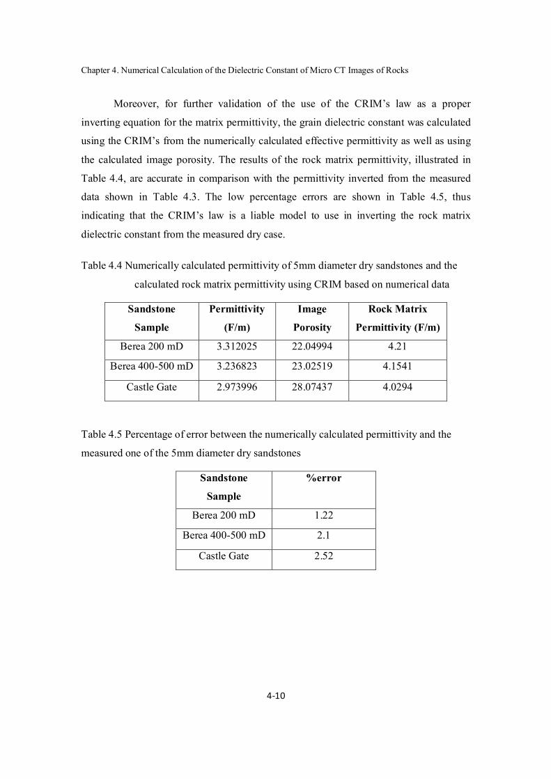
Chapter 4. Numerical Calculation of the Dielectric Constant of Micro CT Images of Rocks
4-10
Moreover, for further validation of the use of the CRIM’s law as a proper
inverting equation for the matrix permittivity, the grain dielectric constant was calculated
using the CRIM’s from the numerically calculated effective permittivity as well as using
the calculated image porosity. The results of the rock matrix permittivity, illustrated in
Table 4.4, are accurate in comparison with the permittivity inverted from the measured
data shown in Table 4.3. The low percentage errors are shown in Table 4.5, thus
indicating that the CRIM’s law is a liable model to use in inverting the rock matrix
dielectric constant from the measured dry case.
Table 4.4 Numerically calculated permittivity of 5mm diameter dry sandstones and the
calculated rock matrix permittivity using CRIM based on numerical data
Sandstone
Sample
Permittivity
(F/m)
Image
Porosity
Rock Matrix
Permittivity (F/m)
Berea 200 mD 3.312025 22.04994 4.21
Berea 400-500 mD 3.236823 23.02519 4.1541
Castle Gate 2.973996 28.07437 4.0294
Table 4.5 Percentage of error between the numerically calculated permittivity and the
measured one of the 5mm diameter dry sandstones
Sandstone
Sample
%error
Berea 200 mD 1.22
Berea 400-500 mD 2.1
Castle Gate 2.52

Chapter 4. Numerical Calculation of the Dielectric Constant of Micro CT Images of Rocks
4-11
Table 4.6 Percentage of error between the rock matrix permittivity derived from the
numerical simulation and the measured one of the 5mm diameter dry sandstones
Sandstone
Sample
%error
Berea 200 mD 1.53
Berea 400-500 mD 2.36
Castle Gate 3.51
Table 4.7 Numerically calculated permittivity of 5mm diameter 100 % saturated low
salinity brine sandstones
Sandstone Sample Permittivity (F/m) Image Porosity
Berea 200 mD 12.99086 22.04994
Berea 400-500 mD 13.09229 23.02519
Castle Gate 14.23178 28.07437
Finally, the permittivity of the two Berea sandstones saturated with deionized
water was measured and presented in Table 4.2. Measurement for the Castle Gate was not
obtainable because the sample ended up being broken. Further attempts in drilling a 5mm
plug of Castle Gate were carried without success due to the extreme material fragility.
Operating at such high frequencies, the permittivity is independent of geometry.
As a result, if the porosity of the image subsets is close to the actual one, and if the
permittivity of the matrix in the numerical calculation is assigned as the true permittivity
of the sandstone under test, the numerical results should be the same as the measured data
for 100% saturated brine sandstones. That can be clearly seen by comparing the measured
data in Table 4.2 with the numerical results in Table 4.7 respectively, where both
converge.
It has been proven by Myers, et al. [3] that the dielectric constant of carbonates
saturated with a fairly low salinity brine fits the Hanai-Bruggeman equation

Chapter 4. Numerical Calculation of the Dielectric Constant of Micro CT Images of Rocks
4-12
with a single depolarization factor “L.” This despite the huge variation in the porosities
and pore space structure between the samples tested, thus illustrating the low sensitivity
of permittivity to geometry at high frequencies. Therefore, in an attempt to further prove
the accuracy of the FDM numerical algorithm used and the possibility of deriving some
petro-physical properties from it, the depolarization factor for each sample was inverted
from the Hanai-Bruggeman equation. Its values are shown in Table 4.8 below. Similar
computation was done from the measured data shown in Table 4.9 below.
It appears that despite the variation in geometry of the samples, the measured
permittivity of the Berea sandstones fits the equation with roughly the same factor, 0.355.
This illustrates the low sensitivity of permittivity to geometry at high frequencies in the
case of sandstone, the same conclusion that Dr. Michael Myers came up with for
carbonates. Moreover, the factor calculated from the measured data is roughly the same
as that derived from the numerical calculations in the case of Berea 400 mD, but a bit
undervalued in case of Berea 200 mD with a 5% error. As for the Castle Gate, no
measured data was possible to obtain due to the extreme fragility of the material.
Therefore no 1-inch long plugs were able to be drilled, and the only existing plug broke
upon saturation. Furthermore, the data obtained for the dry Castle Gate, which resulted in
3.051 F/m of permittivity, is undervalued since the plug was way below one inch, and the
height discrepancy wouldn’t be possible to compensate for it with aluminum foil. This
resulted in an inaccurate measurement of the dry rock dielectric constant for that case,
leading to an inaccurate rock matrix permittivity inverted from the complex refractive
index method law, which lead to a wrong effective permittivity in the numerical
calculation with 100% water saturation. This explains why the derived depolarization
factor for Castle Gate is at a huge offset from that of the Berea sandstones, which tend to
converge in the measured case and is fairly close in the numerical data with less than 5%
error.

Chapter 4. Numerical Calculation of the Dielectric Constant of Micro CT Images of Rocks
4-13
Table 4.8 Depolarization factor of the sandstones inverted from the
numerical data in Table 4.7
Sandstone Sample HB - L factor
Berea 200 mD 0.3381
Berea 400-500 mD 0.3564
Castle Gate 0.4160
Table 4.9 Depolarization factor of the sandstones inverted from the
measured data in Table 4.7
Sandstone Sample HB - L factor
Berea 200 mD 0.3571
Berea 400-500 mD 0.3549
4.4 Conclusions To achieve more accurate numerical results, especially as the project starts to
involve the effect of salinity on the dielectric constant, one needs to build the nonlinear
anisotropic diffusion filter in addition to the segmentation code, thus removing the errors
from the image and clearly separating the pore space from the grain space. As a result
one can obtain in this simulation reliable data that would illustrate the effect of geometry
and various water saturations on the dielectric constant.

Chapter 4. Numerical Calculation of the Dielectric Constant of Micro CT Images of Rocks
4-14
References
1. K. Assami, “Dielectric dispersion in biological cells of complex geometry
simulated by the three dimensional finite difference method,” Journal of Physics:
Applied Physics, Vol. 39, pp.492-499, 2006.
2. M. Luo and C. Liu, “Explanation of dielectric enhancement of some composite
media by a 3D-FDM method,” Society of Exploration Geophysicists, Vol. 28, p.
2184, 2009.
3. M. T. Myers, “A pore geometry dependent dispersion model for the dielectric
constant,” SCA, Paper 9626, 1996.

Study of Array Dielectric Logging Tools
5-1
CHAPTER 5
Study of Array Dielectric Logging Tools Abstract
Dielectric measurement plays a vital role in distinguishing fresh water and carbonates.
For thinly laminated shale oil/gas detection, it could be of great use. Array dielectric
logging tools possesses both longitudinal and transverse polarization antennas which can
be operated at multiple frequencies. We perform detailed investigation on this tool,
demonstrating theoretical derivation of the tool response in cases of homogeneous and
layered formation. Anisotropy is also considered in this study. Meanwhile, results from
numeric simulation are presented. Homogeneous isotropic and anisotropic formations are
taken as examples, both vertically and radically layered cases are covered. In addition,
limitations of the current technology is shed some light on. With profound understanding
of the tool, we hope to achieve development in detecting shale oil/gas with it in the future.
1. Introduction
Reservoir rocks are mostly sedimentary in nature. They consist of a grain and cement
rock matrix with interconnecting void spaces (pores). The pores are filled with formation
water, oil, and gas. Resistivity logging is based on the fact that formation rocks can
transmit an electric current through the absorbed saline water contained inside their pores,
but not through the insulating matrix, oil, and gas. Consequently, water bearing
formations tend to have low electric resistivity relative to hydrocarbon bearing formation.
However, once the pores reach a high resistance of formation fluid such as fresh water,
the resistivity logging tools fail to perform an accurate formation evaluation and provide
incorrect formation property measurements. This is of particularly importance in shale oil
or gas exploration, to determine whether it is oil or fresh water filled in the thin porous
laminated layers. Table 1 lists relative dielectric constants of a number of substances
commonly found in earth formations. Note that rock dielectric constants are independent
of salinity.

Study of Array Dielectric Logging Tools
5-2
Table 1 Dielectric constants of commonly found in earth formations. Substance Relative dielectric constant Limestonea 5.55 Berea sandstonea 3.45 Yule marblea 8.06 Dolomitea 7.92 Pine prairie salta 5.51 Waterb 76.7 Petroleum oilsb 1.92 – 2.22 (a) Values reported by Tam [2] at frequency = 1.0 GHz for dry rocks at room
temperatures. (b) Values reported by von Hipple [3] at frequency = 3.0 GHz and T = 25°C.
Dielectric constant logging was developed in the 1970’s in order to make a distinction
between fresh water and oil, which was difficult to do with resistivity logs alone. Due to
its fairly sensitive measurement of formation water content without knowledge of the
water salinity, interests on it have been growing in industry. Service companies such as
Halliburton, BakerHueghsand Schlumberger all have developed their own dielectric tools.
Most recent dielectric tools are single frequencies around 1GHz with one or two
transmitters, one or two receivers. The performances of such single frequency tools have
been well studied. The array dielectric logging tool is known for its extensive
applications since it possesses multiple frequency channels, various combinations of
transmitter and receiver sets. The performance of the array dielectric logging tool has not
been very clear. Figure 1 is the array dielectric logging tool that consists of two
transmitting antennas and eight receiving antennas symmetrically surrounding the
transmitting antennas. Each antenna is a cross-dipole offering collocated normal
magnetic dipoles working in longitudinal and transversal modes. This tool can be
operated at 20 MHz, 200 MHz, 500 MHz and 1 GHz.
In this report, we perform most of the calculation based on Dielectric logging arrays,
modeling transmitters and receivers as unit moment magnetic dipoles and computing the
tool responses. Section 2 is a presentation of a brief mathematical derivation. After that,

Study of Array Dielectric Logging Tools
5-3
specific cases are considered. Examples include homogeneous isotropic and anisotropic
formation, symmetrically horizontal layered cases and formation with an adjacent layer
of mudcake. The calculated results are displayed and compared with commercial
software simulations in Section 3. Then comes to discussion and conclusion, which is the
last part of the report.
Figure 1. Schematic of Dielectric logging array
2. Formulation
The tool transmitters and receivers are modeled as unit moment magnetic dipoles, which
can generate electromagnetic field in surrounding media. Field distribution depends on
media properties; thus the received signal reflects media parameters such as conductivity
and dielectric constant. The array dielectric logging tool is placed vertically and pushed
tightly against the borehole wall; so dipping is not considered in our discussion. The two
transmitters are in the center of a highly conductive pad, 8 receivers are aligned with
transmitters, located symmetrically above and below. See Figure 1. Given certain spacing,
tool response is defined as

Study of Array Dielectric Logging Tools
5-4
ln A A B B
A B B A
R T R TLG LG
R T R T
S SAT iPS
S S (1)
where A AR TS ,
B AR TS , A BR TS ,
B BR TS denotes response at the receiver described by the
subscript according to corresponding transmitter. As a result of the symmetric geometry
and simplified dipole model, A AR TS =
B BR TS and B AR TS =
A BR TS . The final result is just ratio of
H field at two spacing expressed in logarithm values.
In this part, we evaluate tool response in four cases separately. They are homogeneous
isotropic and anisotropic, vertical and radial layered formations. Schematics of these four
formations are shown in Figure 2, red arrow represents horizontal dipole and blue one
represents longitudinal dipole.
2.1 Homogeneous formation
The H field due to magnetic dipole has been derived from previous work.
퐻 = + 푖푘 푠 − 1 + 3 − 3푖푘 푠 − 푘 푠 − −
2푖푘ℎ푥2휌4−푖푘ℎ푟2+푘ℎ2푥2+1푟3+3푖푘ℎ푥2푟4−3푥2푟5 (2)
퐻 = 푘 푟 + 푖푘 푟 − 1 + 3 − 3푖푘 푟 − 푘 푟 (3)
Here, /h v is an anisotropic coefficient and s is related to λ. For isotropic
formation, λ=1. The tool is located along vertical axis, thus x=0, y=0, ρ=0. Cross
components are zero. Equation (2) and (3) can be simplified as 2
2 3
1( )4
hik rh h
xxk ikeHr r r
(4)
2
22( )4
hik rh
zzikeH
r r r (5)
Thus, tool response can be obtained from

Study of Array Dielectric Logging Tools
5-5
2 2
2 2
1 1 ( / 2) ( / 2)/ 23ln( ) ln[ ]/ 2 1 1 ( / 2) ( / 2)
h hxx xx h
h h
ik r k rrAT iPS ikr ik r k r
(6)
1 1 ( / 2)/ 23ln( ) ln[ ]/ 2 1 1 ( / 2)
hzz zz h
h
ik rrAT iPS ikr ik r
(7)
For anisotropic formation, Hzz stays the same, and Hxx reflects the anisotropy factor.

Study of Array Dielectric Logging Tools
5-6
Figure 2. Four cases of the formation structures to be investigated: (a) Homogeneous
isotropic formation (b) Homogeneous anisotropic formation (c) Vertically layered
formations and (d) Formation with radial-directed mudcakes
Rv
Rh
T
R1
R2
Rv
Rh
T
R1
R2
Rv
Rh
T
R1
R2
(a) (b)
(c) (d)
h v
r r
h v
2 2 2, ,h v r
3 3 3, ,h v r
4 4 4, ,h v r
T
R1
R2
mudcake
formation
borehole borehole

Study of Array Dielectric Logging Tools
5-7
Since Hzz does not reflect anisotropy, the formula in anisotropic formation stays the
same with isotropic cases. But Hxx is expressed as
2 2
2 2
1 1 ( / 2) ( / 2)/ 23ln( ) ln[ ]/ 2 1 1 ( / 2) ( / 2)
h vxx xx h
h v
ik r k rrAT iPS ikr ik r k r
(8)
2.2. Inhomogeneous cases
a) Formation with a layer of mudcake
Pushed against the borehole wall, both longitudinal and transverse transmitters are
parallel to the mudcake and formation plane. Based on published papers, H field detected
by the receiver is derived as:
11
ˆ ( )2
i xiH d e g
(9)
where 1
1
12 11 2
1 12 1
2 ( )( ) [1 ]1 ( )
i h
i h
eige
221 1 2
12 1 221 1 2
( ) nn
2 21 1k
2 22 2k
1,2 1/21,2 1,2 0
1,2
(1 )k i
Since it is not obvious to obtain a close form expression, we integrate numerically H field
at each receiver separately and acquire tool response via the ratio.
b) Symmetrically vertical layered formation
Antenna on array dielectric logging tool is placed on a conductive pad which can be
regarded as a perfect conductor. For symmetric 1D formation, field is symmetric about
the tool. Apply equivalence theorem, tool response in the interested zone are just twice of
that without the pad. The case without pad has been completely studied in publications of
Study of Array Dielectric Logging Tools
5-8
Well Logging Laboratory. Major calculating steps as explained in this section. To be
general, ̂ is a complex conductivity tensor defined by
ii
i
v
h
h
000000
ˆ (10)
We can introduce the Hertz vector potential Π and scalar potential to express electric
and magnetic fields
1E hi (11)
hi 0H (12)
Substituting (8) and (9) into equations (5) and (6), we obtain
.10
0sME
hii
(10)
We introduce a gauge condition for the scalar potential,
.ˆ v (11)
Substituting (8) and (11) into equation (10), we obtain
sMb h
v
i 02 ˆ1 (12)
where b is a matrix defined by
b =
yxz
z
z
yx
y
x
)1(
)1(
)1(
2
22
2
22
2
(13)
Equation (12) can be written as three scalar equations:

Study of Array Dielectric Logging Tools
5-9
,11202
2
22
2
2
2
xxvxxx Mi
zyx
(14)
,11202
2
22
2
2
2
yyvyyy Mi
zyx
(15)
zhzzz i
zyx
02
2
2
2
2
2
yxz
M yxz
21 . (16)
Equation (14)-(16) can be rewritten in a new form
xxvx Mk 222 1
(17)
yyvy Mk 222 1
(18)
,1 222
yxz
Mk yxzzhz
(19)
where
2
2
22
2
2
22 1
zyx , and hh ik 02 and vv ik 0
2 .
Equations (17)-(19) are scalar equations of the potentials and make it possible to treat the
source components xM , yM and zM separately. The solution in multi-layered with an
ideal vertical magnetic dipole is discussed in this report and corresponding magnetic field
response can be found thereafter.

Study of Array Dielectric Logging Tools
5-10
Fig 3 A vertical magnetic dipole in multi-layered formation
According to equations (17) - (19), with only the z-directional coil, resulting potential
have only z component zi in each layer. In ith layer of anisotropic layered formation, i.e
z < 푧 < z , zi can be written in the following form, where Fi and Gi are transmission
and reflection coefficient representing upgoing and downgoing elecro-magnetic waves
respectively.
And
ξ = (λ − k ) / (λ + k ) /
k = (jωμ σ ) /
Jn(x) is the nth order Bessel function and
β = 0, ifMisnotinlayeri1,ifMisinlayeri
�
Now consider boundary conditions at z=zi . The electrical field can be express as 1ˆhj
E .
Substituting ˆz z into the above equation, we get
hi hi hiξ |z| ξ z ξ zz izi i i 1
hi0
M βπ ( e Fe G e ) J ρ d4π ξ

Study of Array Dielectric Logging Tools
5-11
1ˆ ˆ ˆz zhj x y
x y
E .
From the continuity of tangential component of electrical field at the interface of the i-th
and i+1-th layer, explicitly
1xi x iE E ; 1yi y iE E ,
We can get
1 1i zi i z i .
The magnetic field can be express as
ˆ
hv
j
H
0 0 0
ˆ 0 0 00 0 1
h z
z
j z
2 2 2
2ˆ ˆˆ ˆz z zh zj z x y z
x z y z z
.
From the continuity of tangential component of magnetic field at the interface of the i-th
and i+1-th layer, we can obtain
( 1)z izi
z z
Followed by potential expression and boundary conditions, solving for Fi and Gi is the
next step. Assume there are N layers in total, and the transmitter is in ith layer. We define
a coefficient vector Ui=[Fi Gi]T. Obviously, there is no downgoing wave in the
uppermost layer or upgoing wave in the bottom layer. This can be expressed as
U = [F , 0] , U = [0, G ] .
A simpler case would be two adjacent layers without source
( 1) ( 1)
( 1) ( 1)
( ) ( )111 21
( ) ( )121 22
hk h k k hk h k k
hk h k k hk h k k
z zk k
z zk k
F Fp e p eG Gp e p e
Study of Array Dielectric Logging Tools
5-12
where
11 1 ( 1) 22
12 1 ( 1) 21
0.5( / / )
0.5( / / )k k h k hk
k k h k hk
p pp p
For those three layers sandwiches in the transmitter, contribution of the source need to be
calculated
( 1) ( 1)
( 1) ( 1)
( 1) ( 1)
( ) ( )111 21 1
( ) ( )1 221 22
( ) ( )1 12 2 22
(1 11
1
1 1,
hi h i i hi h i i
hi h i i hi h i i
hi h i i hi h i i
z z ii i
iz zi i
z zi i
hi hi
i
i
F Fp e p e sG G sp e p e
s p e s p e
F p eG
( 1) 1 ( 1) 1
( 1) 1 ( 1) 1
( 1) 1 ( 1) 1
) ( ) 121 1
1( ) ( )221 22
( ) ( )1 11 12 2 11
1 1,
h i hi i h i hi i
h i hi i h i hi i
h i hi i h i hi i
z z ii
iz zi
z zi i
hi hi
Fp e sG sp e p e
s p e s p e
For simplicity, we define ei, Si and Si+1
1 2
Ti iiS s s , and
1 11 2
Ti iiS s s
( 1)
( 1)
( )
( )
1
hi h i i
hi h i i
z
iz
ee
e
In summary, we have the iteration expression of the coefficient:
퐔 = e 퐏퐔 + e 퐒 forz ≥ 0
퐔 = e 퐏퐔 + 퐒 forz < 0
Together with the fact that F and G are zero, final expression of Hertz potential caused
by the vertical coil can be derived. As a result, Hxz, Hyz, Hzz is obtained. It is similar
case with transverse coils; so we omit the trivial derivation.
3. Numerical Results
Numerical results of the above examples are displayed in this section. Tool response with
respect to formation properties such as conductivity and relative dielectric constant are

Study of Array Dielectric Logging Tools
5-13
plotted. Note that the spacing between transmitters and receivers are assumed to be the
same for all the antennas due to limited public knowledge of the tool structure.
a. Homogeneous formation
The tool can operate at 20 MHz, 500 MHz and 1GHz. Lower frequency channel is more
sensitive to conductive variation while higher frequency response indicates more
information of dielectric constant. Meanwhile, all the responses are monotonous with
respect to σ and εr regardless of the frequency. Since the formation is simple, all the
useful information can be extracted from Hzz alone. The next a few graphs are AT and
PS in the z direction at various frequencies. For anisotropic case, only x-directional
response is presented as we mentioned that Hzz is exactly the same with isotropic
formation. 20 MHz and 1 GHz are used in this case to plot ATx and PSx v.s. conductivity
and relative dielectric constant respectively. To get the plot of conductivity, relative
dielectric constant is assumed as 15 and ratio between transverse and vertical
conductivity is a constant 5. When dielectric constant is the variable, conductivity is set
as 0.6 / , 0.1 /h vS m S m . See Figure 4 and Figure 5.

Study of Array Dielectric Logging Tools
5-14
(a)
(b)
0 10 20 30 40 50 60 70 80 900.55
0.6
0.65
0.7
0.75
0.8
0.85
0.9
0.95
1
1.05longitudinal attenuation in homogeneous isotropic formation
r
ATz
LG
v=h=0.6S/m r=3 inch
r=4 inchr=5 inchr=6 inch
0 10 20 30 40 50 60 70 80 900.105
0.11
0.115
0.12
0.125
0.13
0.135
0.14
0.145
0.15
0.155longitudinal phase shift in homogeneous isotropic formation
r
PS
z LG
v=h=0.6S/m r=3 inch
r=4 inchr=5 inchr=6 inch

Study of Array Dielectric Logging Tools
5-15
(c)
(d)
10-3 10-2 10-1 100 1010.4
0.5
0.6
0.7
0.8
0.9
1
1.1
1.2
1.3longitudinal attenuation in homogeneous isotropic formation
/(S/m)
ATz
LG
r=15 r=3 inchr=4 inchr=5 inchr=6 inch
10-3
10-2
10-1
100
101
0
0.05
0.1
0.15
0.2
0.25
0.3
0.35longitudinal phase shift in homogeneous isotropic formation
/(S/m)
PS
z LG
r=15 r=3 inchr=4 inchr=5 inchr=6 inch

Study of Array Dielectric Logging Tools
5-16
(e)
(f)
0 10 20 30 40 50 60 70 80 90
0.7
0.8
0.9
1
1.1
1.2
1.3
1.4
1.5
1.6longitudinal attenuation in homogeneous isotropic formation
r
ATz
LG
v=h=0.6S/m r=3 inch
r=4 inchr=5 inchr=6 inch
0 10 20 30 40 50 60 70 80 900.8
1
1.2
1.4
1.6
1.8
2
2.2
2.4
2.6longitudinal phase shift in homogeneous isotropic formation
r
PS
z LG
v=h=0.6S/m r=3 inch
r=4 inchr=5 inchr=6 inch

Study of Array Dielectric Logging Tools
5-17
(g)
(h)
10-3
10-2
10-1
100
101
0.2
0.4
0.6
0.8
1
1.2
1.4
1.6
1.8
2
2.2longitudinal attenuation in homogeneous isotropic formation
/(S/m)
ATz
LG
r=15 r=3 inch
r=4 inchr=5 inchr=6 inch
10-3 10-2 10-1 100 1010.9
1
1.1
1.2
1.3
1.4
1.5
1.6
1.7
1.8longitudinal phase shift in homogeneous isotropic formation
/(S/m)
PS
z LG
r=15 r=3 inchr=4 inchr=5 inchr=6 inch

Study of Array Dielectric Logging Tools
5-18
(i)
(j)
0 10 20 30 40 50 60 70 80 90
0.8
1
1.2
1.4
1.6
1.8
2longitudinal attenuation in homogeneous isotropic formation
r
ATz
LG
v=h=0.6S/m r=3 inchr=4 inchr=5 inchr=6 inch
0 10 20 30 40 50 60 70 80 901
1.5
2
2.5
3
3.5
4
4.5
5longitudinal phase shift in homogeneous isotropic formation
r
PS
z LG
v=h=0.6S/m r=3 inchr=4 inchr=5 inchr=6 inch

Study of Array Dielectric Logging Tools
5-19
(k)
(l)
Figure 4. Tool response in homogeneous isotropic formation when the antenna spacing is
1 inch for all antennas. Conductivity is 0.6 S/m for relative dielectric constant variation,
and relative dielectric constant is 15 for changing conductivity. (a)-(d). Longitudinal tool
10-3
10-2
10-1
100
101
0
0.5
1
1.5
2
2.5
3longitudinal attenuation in homogeneous isotropic formation
/(S/m)
ATz
LG
r=15 r=3 inch
r=4 inchr=5 inchr=6 inch
10-3
10-2
10-1
100
101
2
2.1
2.2
2.3
2.4
2.5
2.6
2.7
2.8longitudinal phase shift in homogeneous isotropic formation
/(S/m)
PS
z LG
r=15r=3 inchr=4 inchr=5 inchr=6 inch

Study of Array Dielectric Logging Tools
5-20
response at 20 MHz. (e)-(h). Longitudinal tool response at 500 MHz. (i)-(l).
Longitudinal tool response at 1 GHz.
(a)
10-3
10-2
10-1
100
101
0.2
0.4
0.6
0.8
1
1.2
1.4
1.6transverse attenuation in homogeneous isotropic formation
h/(S/m)
ATx
LG
r=15,h/v=5 r=3 inchr=4 inchr=5 inchr=6 inch

Study of Array Dielectric Logging Tools
5-21
(b)
(c)
10-3
10-2
10-1
100
101
0
0.5
1
1.5transverse phase shift in homogeneous isotropic formation
h/(S/m)
PS
x LG
r=15,h/v=5 r=3 inch
r=4 inchr=5 inchr=6 inch
0 10 20 30 40 50 60 70 80 900
0.2
0.4
0.6
0.8
1
1.2
1.4
1.6
1.8transverse attenuation in homogeneous isotropic formation
r
ATx
LG
v=0.1S/m,h=0.6S/m r=3 inch
r=4 inchr=5 inchr=6 inch

Study of Array Dielectric Logging Tools
5-22
(d)
Figure 5. Transverse response in homogeneous anisotropic formation. (a), (b) ATx and
PSx with respect to conductivity at 20 MHz. (c), (d) ATx and PSx with respect to relative
dielectric constant at 1 GHz
b. Formation with mudcake
See Figure 2 (d) for the schematic of the tool in the formation. Antennas in both
directions are parallel with the formation and mudcake plane. Assume both the mudcake
and formations are isotropic; responses in two directions are identical. Keep relative
dielectric constant as changing variable, AT and PS are simulated with constant
tangential loss. Working frequency is 1 GHz. The results of dielectric constant range
from 5-25 are compared with published paper.
0 10 20 30 40 50 60 70 80 902
2.5
3
3.5
4
4.5
5transverse phase shift in homogeneous isotropic formation
r
PS
x LG
v=0.1S/m,h=0.6S/m r=3 inch
r=4 inchr=5 inchr=6 inch

Study of Array Dielectric Logging Tools
5-23
(a)
(b)
0 10 20 30 40 50 60 70 80 90 10011.8
12
12.2
12.4
12.6
12.8
13
13.2
13.4
13.6
13.8
r
AT
attenuation of tool with mudcake rm=25, tanm=1
tan=0.1tan=0.3tan=0.4tan=0.6
0 10 20 30 40 50 60 70 80 90 100-4
-3
-2
-1
0
1
2
3
4
r
PS
phase of tool with mudcake rm=25, tanm=1
tan=0.1tan=0.3tan=0.4tan=0.6

Study of Array Dielectric Logging Tools
5-24
(c)
Figure 6. Simulated tool response in isotropic formation and mudcake. (a) AT (b) PS (c)
Error compared with publish paper
c. Layered formation
Numeric simulation of tool response in laminated formations is performed and displayed
in the next a few graphs. Three examples are provided:
Example 1: 5 layer formation, each layer has the same conductivity, 0.6 /h v S m ,
dielectric constant are 1, 7, 15, 51, 7 from top to bottom layers. The tool is set working at
1 GHz. See Figure 7 for formation structure and numeric results.
Example 2: 5 layer formation, each layer has the same relative dielectric constant of 15.
Horizontal and vertical conductivity are the same; from top to bottom layers are 0.1 S/m,
1 S/m, 0.5 S/m, 0.2 S/m, and 0.01 S/m respectively. The tool is set working at 20 MHz.
See Figure 8 for formation structure and numeric results.
0.00%
0.50%
1.00%
1.50%
2.00%
2.50%
3.00%
3.50%
4.00%
0.1 0.1 0.1 0.1 0.1 0.3 0.3 0.3 0.3 0.3 0.4 0.4 0.4 0.4 0.4 0.6 0.6 0.6 0.6 0.6
5 10 15 20 25 5 10 15 20 25 5 10 15 20 25 5 10 15 20 25
Formation Parameters
Error in Observed values
d = 0 cm
d = 0.3 cm
d = 0.5 cm
d = 1.0 cm

Study of Array Dielectric Logging Tools
5-25
Example 3: 5 layered isotropic formation. Conductivity of each layer is shown in Figure
9 (a). Tool response at 20 MHz and 1 GHz against r are plotted.
(a)
0 10 20 30 40 50 60
00.5
2
5
r
dept
h/fo
ot
Layered isotropic formation
-4 -3 -2 -1 0 1 2 3
00.5
2
5
AT
dept
h/fo
ot
Layered isotropic formation attenuation
Z directionX direction
-8 -6 -4 -2 0 2 4
00.5
2
5
PS
dept
h/fo
ot
Layered isotropic formation phase
Z directionX direction

Study of Array Dielectric Logging Tools
5-26
(b) (c)
Figure 7 Array dielectric logging tool response in layered isotropic formation (f=1 GHz)
(a)
10-2
10-1
100
00.5
2
5
/<S/m>
dept
h/(fo
ot)
Layered formation Conductivity
-0.5 -0.4 -0.3 -0.2 -0.1 0 0.1 0.2 0.3
00.5
2
5
PS
dept
h/fo
ot
Layered isotropic formation phase
Z directionX direction
3.1 3.15 3.2 3.25 3.3 3.35 3.4 3.45 3.5
00.5
2
5
AT
dept
h/fo
ot
Layered isotropic formation attenuation
Z directionX direction

Study of Array Dielectric Logging Tools
5-27
(b) (d)
Figure 8. Array dielectric logging tool response in layered isotropic formation (f=20
MHz)
(a)
10-2
10-1
100
00.5
2
5
dept
h/fo
ot
Layered anisotropic formation(r=15)
h
v
-16 -14 -12 -10 -8 -6 -4 -2 0 2 4
00.5
2
5
AT
dept
h/fo
ot
Layered anisotropic formation attenuation
Z directionX direction
-10 -5 0 5 10 15
00.5
2
5
PS
dept
h/fo
ot
Layered anisotropic formation phase
Z directionX direction

Study of Array Dielectric Logging Tools
5-28
(b) (c)
(d) (e)
Figure 8. Array dielectric logging tool response in layered anisotropic formation (a)
Formation structure. (b) and (c) Tool response at f=1 GHz (d) and (e) Tool response
at f= 20 MHz
4. Conclusions
From previous discussion, we can conclude that array dielectric logging tool behaves
well in detecting various formation structures, isotropic or anisotropic, homogeneous or
inhomogeneous. Higher frequency channels like 1 GHz are better choice for dielectric
constant exploration; while lower frequencies plays more importance role in conductivity
investigation. Response from longitudinal antenna implies most of the information in
transverse plane; thus is especially useful in homogeneous isotropic formation evaluation.
For more complex media, for example, laminated or radially inhomogeneous formation,
transverse components start to involve and reflect anisotropy factor and boundary
influence. Both components are sensitive to media conductivity and relative dielectric
constant. Utilizing different combinations of antenna spacing and frequency channel, the
tool can detect thin layers within 0.5 inches.
1.8 2 2.2 2.4 2.6 2.8 3 3.2 3.4 3.6 3.8
00.5
2
5
AT
dept
h/fo
ot
Layered isotropic formation attenuation
Z directionX direction
-3.5 -3 -2.5 -2 -1.5 -1 -0.5 0 0.5 1
00.5
2
5
PS
dept
h/fo
ot
Layered isotropic formation phase
Z directionX direction

Study of Array Dielectric Logging Tools
5-29
Future work will cover more case studies and maybe experimental results. Inversion
algorithm will be developed. We hope it could live up to the expectation of solving the
difficulty in discovering laminated shale oil or gas.

Study of Array Dielectric Logging Tools
5-30
References
[1] S. Calvert and T. Pritchard, BG Group, Eric Decoster, Schlumberger, 2006, “Tri-
axial array induction tool aids field development for the north coast marine area,”
SPWLA 47th Annual Logging Symposium, June 4-7, 2006.
[2] Hanming Wang, “Triaxial Induction Logging -Theory, Modeling, Inversion and
Interpretation,” Well Logging Research Seminar Announcement, University of
Houston, March 24, 2006
[3] Aria Abubakar,1 Tarek M. Habashy,1 Vladimir Druskin,1 Leonid Knizhnerman,2 and
Sofia Davydycheva3, “A 3D parametric inversion algorithm for tri-axial induction
data,” Geophysics, Vol. 71, No. 1, pp. G1–G9, January-February 2006.
[4] Northwest Geophysical Associates, Inc, “Conductivity logs”, GEOPHYSICAL
BOREHOLE LOGGING, November 25, 1997
[5] Barbara Ina Anderson, “Modeling and Inversion Methods for the Interpretation of
Resistivity Logging Tool Response, ”Schlumberger, 2001
[6] Lili Zhong, Jing Li; A. Bhardwaj, L.C. Shen, and R. C. Liu, “Computation of
Triaxial Induction Logging Tools in Layered Anisotropic Dipping Formations,”
IEEE Trans. Geoscience and Remote Sensing, vol. 46, pp.1148 – 1163, 2008.
[7] M. Huang, and L.C. Shen, “Computation of induction logs in multiple-layer
dipping formation,” IEEE Trans. Geoscience and Remote Sensing, vol.27, no.3, pp
259-267, 1989.

A-1
APPENDIX A
List of Theses and Dissertations
The following are senior theses, master theses, and doctoral dissertations completed by
the research staff of the Well Logging Laboratory.
1982 Shabbir A. Chowdhury
Investigation of Electrode Effects in the Measurement of Impedance of Water Saturated Rocks at Low Frequencies (M. S. Thesis) Shey-Min Su Measurements of Dielectric Constant and Conductivity of Petroleum Reservoir Rocks at Microwave Frequencies (M. S. Thesis)
1984 Hardy X. J. Guo
Physical Modelling of Induction Logging in Dipping Beds (M. S. Thesis) S. C. Frank Huang Techniques for Measuring the Dielectric Properties of Samples Using Coaxial-Line and Insulated Antenna (Ph. D. Dissertation) Shahryar Darayan High-Temperature Electromagnetic Properties of Reservoir Rocks at UHF (M. S. Thesis)
1985 Herzl Marouni Dielectric Constant and Conductivity Measurement of Reservoir Rocks in the Range of 20-50 MHz (M. S. Thesis) Gong Li Physical Modelling of Induction Logging in Dipping Beds with a Large Borehole (M. S. Thesis)
1986 Michel S. Bittar
Laterolog Scale Modelling Experiments

A-2
(M. S. Thesis) Nancy S. Pollard Computer Simulation of Induction Tool Resistivity Readings in Multiple Layer Formations (Senior Thesis) Kobina O. Eshun A New Design for the WLL Induction Logging Model Facility (Senior Thesis)
1987 Lee-Hwa Lue Wang
Inversion of Induction Logging Data in Horizontally Layered Formation (M. S. Thesis) Ming Huang Modeling Medium Inhomogeneity in Induction Logging (M. S. Thesis) Xin Lin Microwave Dipmeter (M. S. Thesis)
1988 Kuang-Fu Han Dielectric Constant Measurement of Saline Solution at 1.1 GHz (M. S. Thesis) Muhammad N. A. Ansari Effect of Dissimilar Scale Factors for Length and Diameter on Shallow Laterolog Scale-Model Tool Response (M. S. Thesis) Kobina O. Eshun A Laboratory Model of the Focused Induction Logging Sonde (M. S. Thesis) Chi-Ming Lam Modelling the Electrode Well-Logging Sonde by the Method of Finite Elements (M. S. Thesis) Chia-Hsiang Lin Conductivity Measurement at Low Frequencies Using a Digital Bridge (M. S. Thesis)

A-3
1990 Yongdong He Input Impedance of an Antenna and Its Application in Complex Permittivity Measurement at High Frequencies (Ph. D. Dissertation) Michael S. Bittar Study of Resistivity Sondes by Scale Modeling and Three-Dimensional Finite element Method (Ph. D. Dissertation)
1991 Xiaolu Zhao
Numerical Analysis of a TM010 Cavity for Dielectric Measurement (M. S. Thesis)
1992 Chun-ta Chao
Wellog Simulator: Simulation for Induction Tool in Layered Medium (M. S. Thesis) Yu-zhi Li Monopole Antenna as a Probe for Measuring Dielectric Properties at 300-1100 MHz (M. S. Thesis) Tien-min Wang Electrical Properties of Saline Solution and Contaminated Soils (M. S. Thesis)
1993 Shahryar Darayan
Measurement of Dielectric Permittivity and Conductivity of Samples Using Guarded Electrodes (Ph. D. Dissertation) Ming Huang Resistivity Measurement in Laboratory and Field Environments (Ph. D. Dissertation) Yongchun Zhang Induction Log Inversion and Cross-Hole Electromagnetic Tomography (Ph. D. Dissertation)
1994 Jiazhi Chui
A-4
Simulation of Measurement-While-Drilling Tool in Cylindrical Media (M. S. Thesis) Liang (Linda) Lin Simulation of Induction Tools in Dipping Beds (M. S. Thesis) Yongmin Zhang A Time-Domain Modeling and Inversion Technique and Its Applications to Electromagnetic Subsurface Sensing (Ph. D. Dissertation)
1995 Qian Gu
Evaluation of Approximations Used to Simulate MWD Tools in Layered Formations (M. S. Thesis) Xuhua Hu Radial Resistivity Profile Invasion Using Array Induction Logs (M. S. Thesis) Xiaoning Zhang Quick Look Inversion of Through Casing Resistivity Measurement (M. S. Thesis)
1996 Rohit Gaikwad
Scale Modeling of the Through-Casing Resistivity Tool (M.S. Thesis) Feng Gao A Scale Model of the Through-Casing Resistivity Measurement (M.S. Thesis) Jing Lin Three Dimensional Finite-Element Mesh Generation and Interactive Computer Graphic Visualization System (M. S. Thesis) Xiao-bing Wu Inversion of Induction Logs in Dipping Beds (Ph.D. Dissertation)
Ruilin Zhong

A-5
Simulation the Effects of Casing Corrosion on the Through-Casing Resistivity Logs (M. S. Thesis) Jiang Zhu Modeling and Evaluation of MWD Resistivity Tool in Horizontal Well (M. S. Thesis)
1997 Ji Fang
Algorithms for Inversion of Induction Logs in Dipping Bed (M. S. Thesis)
Xiang Tian Numerical Simulations of Induction and MWD Logging Tools and Data Inversion Method with X-Window Interface on a UNIX Workstation (Ph.D. Dissertation) Yuanzheng Ming Simulation of Through-Casing Resistivity Logging (M. S. Thesis) Hongxu Wu Theoretical Studey of the Effective Dielectric Constant of 3D Mixtures with Applications in Soil Water Content Measurement (M.S. Thesis)
1998 Jingjing Sun
Simulation of Induction Logging in 2D Formation using the Born Approximation (M. S. Thesis) Shu Huang Computer Simulation of Microwave Flow Meter (M. S. Thesis) Long Wang 3-D Numerical Modeling of Induction Resistivity Tool for Well Logging Using Finite Element Method (Ph.D. Dissertation)
1999 Huage Zheng Physical Modeling of an Automated Through-Casing Resistivity Measurement System

A-6
(M. S. Thesis) Hanming Wang Finite Element Analysis of Resistivity Logging (Ph.D. Dissertation)
2000 Yuan Hu
Simulation of Induction and MWD Logging in Wells with Varying Dip Angles (M. S. Thesis) Jian Li 2-D Inversion for Induction and MWD Logs (Ph.D. Dissertation)
Ji Li Modeling Electrode-type Logging Tools in 2-D Formations by Finite Element Method (M. S. Thesis) Guoyu Hu Two-dimensional Cross-well Forward Modeling and Inversion (M. S. Thesis)
2001 Chatrpol Lertsirimit
Apparatus for Measuring Conductivity Tensor of Anisotropic Samples in the Laboratory (M. S. Thesis) Chuanxiao Li A Graphical Interface for Well-Logging Codes (M. S. Thesis)
2002 Pei Jin
Laboratory Technique for Measuring Conductivity Tensor of Anisotropic Samples (M. S. Thesis) Lili Zhong Simulation of Multi-Component Induction Tool in Dipping Beds (M. S. Thesis) Wei Gao 3D Transmission Line Matrix Method and Application Interface (M. S. Thesis)

A-7
2004 Lili Zhong
Simulation of Tri-Axial Induction Tools in Dipping Anisotropic Beds (Ph.D. Dissertation) Shanjun Li Analysis of Complex Formations Using Computer Techniques (Ph.D. Dissertation) Weishan Han 3D Finite Element Simulation Method of Induction and MWD Tools (Ph.D. Dissertation)
2005 Jing Li
Electrical Property Measurement of Rocks in the Range of 10kHz –1.1GHz (M.S. Thesis)
2006 Xueshen Yu Inversion of Tri-Axial Induction Logs in Anisotropic Formation (M.S. Thesis)
2007 David Navarro Effects of Invasion Transient on Resistivity Time-Lapsed Logging (M.S. Thesis)
2008 Asutosh Bhardwaj 1-D Inversion of Tri-axial Induction Logs in Anisotropic Medium (M.S. Thesis)
Yumei Tang Modeling and Inversion of Multicomponent Induction Logs in Biaxial Anisotropic Formation (Ph.D. Dissertation)
2009 Li Zhong
Response of Induction and LWD Tools in Multiple Cylindrically Layered Media (M.S. Thesis) Jinjuan Zhou Application of Finite Element Method in Solving Well Logging Problems (Ph.D. Dissertation)

A-8
Hamid Naseri Electromagnetic Telemetry in Measurement-While-Drilling with a Wireless Relay Network (Ph.D. Dissertation) Mark Collins Response of MWD Resistivity Tools in Eccentric Cylindrically Layered Media (M.S. Thesis)
2010 Huaping Wang Ground Penetrating Radar with Wireless Data Access and Control (Ph. D. Dissertation) Wei Ren The Portable Ground Penetrating Radar System Design (Ph.D. Dissertation)
Chen Guo Research on Ultra Wideband(UWB) Antenna and Radar Application (Ph.D. Dissertation)
2011
Zhijuan Zhang 1D Modeling and Inversion of Triaxial Induction Logging Tools in Layered Anisotropic Medium (Ph.D Dissertation) El Emir Fouad Shehab Large Dielectric Enhancement Measurement at Low Frequencies and Numerical Evaluation of Permittivity of Digital Rocks at High Frequency (MS Thesis) Yinan Xing Road Profiling System using Non-contact laser Displacement Sensor (MS Thesis) Guoyu Hu Analysis of Induction Tool Response to Fractures Using an Improved 3D Finite Difference Method (Ph.D Dissertation)

A-9
2012 Changmin Lin Study of Dielectric Constant Logging Tools (MS Thesis) Yajuan Kong Study of Logging-While-Drilling Simulation Models Using Wellog Inversion Software and COMSOL (MS Thesis) Ziting Liu Wireless MWD Telemetry System Using MEMS Radio (MS Thesis)

B-1
APPENDIX B
List of Technical Paper Publications
The following are papers published in technical journals and symposium transactions by
the research staff of the Well Logging Laboratory.
Papers Published in Technical Journals 1983
F.S.C. Huang and L. C. Shen, “Analysis of error due to presence of gaps in the measurement of rock samples in a coaxial Line,” Geophysics, Vol.48, No.2, pp.206-212, February 1983.
1984
G. J. Zhang and L. C. Shen, “Response of a normal resistivity tool in a borehole crossing a bed boundary,” Geophysics, Vol. 49, No. 2, pp. 142-149, February 1984. D. Coope, L. C. Shen, and F. S. C. Huang, “The theory of 2 MHz resistivity tool and its application to measurement-while-drilling,” The Log Analyst, Vol. XXV, No. 3, pp. 35-46, May-June 1984.
1985
L. C. Shen, W. C. Savre, J. M. Price and K. Athavale, “Dielectric properties of reservoir rocks and ultra high frequencies,” Geophysics, Vol. 50, No. 4, pp. 692-704, April 1985. L. C. Shen, “A Laboratory Technique for measuring dielectric properties of core samples at ultra high frequencies,” Society of Petroleum Engineers Journal, pp. 502-514, August 1985. L. C. Shen, and G. J. Zhang, “Electromagnetic field due to a magnetic dipole in a medium containing both planar and cylindrical boundaries,” IEEE Transactions on Geoscience and Remote Sensing, Vol.23, No. 6, pp. 827-833, November 1985. L. C. Shen, “Problems in dielectric-constant logging and possible routes to their solution,” The Log Analyst, Vol. XXVI, No. 6, pp. 14-25, November-December 1985.

B-2
1986
R. H. Hardman and L. C. Shen, “Theory of induction sonde in dipping beds,” Geophysics, Vol. 51, No. 3, pp. 800-809, March 1986.
1987
R. H. Hardman and L. C. Shen, “Charts for correcting the effect of formation dip and hole deviation on induction logs,” The Log Analyst, Vol. 28, No. 4, pp. 349-356, July-August 1987. D. P. Shattuck, Michel Bittar and L. C. Shen, “Scale modelling of the laterolog using synthetic focusing methods,” The Log Analyst, Vol. 28, No. 4, pp. 357-369, July-August 1987. L. C. Shen, H. Marouni, Y. X. Zhang and X. D. Shi, “Analysis of parallel-disk sample holder for dielectric permittivity measurement,” IEEE Transactions on Geoscience and Remote Sensing, Vol. 25, No. 5, pp. 534-540, September 1987.
1989
M. Huang and L. C. Shen, “Computation of induction logs in multiple-layer dipping formation,” IEEE Transactions on Geoscience and Remote Sensing, Vol. 27, No. 3, pp. 259-267, May 1989. L. C. Shen, “Effects of skin-effect correction and three-point deconvolution on induction logs,” The Log Analyst, Vol. 30, No. 4, pp. 217-224, July-August 1989.
1990
L. C. Shen, C. Liu, J. Korringa and K. J. Dunn, “Computation of conductivity and dielectric constant of periodic porous media,” J. of Applied Physics, Vol. 67, No.11, pp. 7071-7081, June 1990. M. S. Bittar, D. P. Shattuck and L. C. Shen, “Laboratory study of the shallow laterolog in high and low contrast zones,” The Log Analyst, Vol. 31, No.4, pp.189-197, 1990.
1991
K. F. Han, C. M. Butler, L. C. Shen, Y. D. He and M. A. Harris, “High-frequency dielectric permittivity of saline solution at elevated temperature,” IEEE

B-3
Transactions on Geoscience and Remote Sensing, Vol.29, No.1, pp. 48-56, January 1991. C. Liu and L. C. Shen, “Response of electromagnetic-pulse logging sonde in axially-symmetrical formation,” IEEE Transactions on Geoscience and Remote Sensing, Vol.29, No.2, pp. 214-221, March 1991. C. Liu and L. C. Shen, “Numerical simulation of subsurface radar for detecting buried pipes,” IEEE Transactions on Geoscience and Remote Sensing, Vol.29, No. 5, pp.795-798, September 1991. L. C. Shen, “Theory of a coil-type resistivity sensor for MWD application,” The Log Analyst, vol. 32, pp. 603-611, No.5, 1991.
1992
Y. D. He and L. C. Shen, “Measurement of complex permittivity of materials using a monopole antenna,” IEEE Transactions on Geoscience and Remote Sensing, Vol.30, No.3, pp. 624-627, May 1992. X. L. Zhao, C. Liu and L. C. Shen, “Numerical analysis of a TM010 cavity for dielectric measurement,” IEEE Transactions on Microwave Theory and Techniques, Vol.40, No.10, pp. 1951-1959, October 1992. J. Li and L. C. Shen, “Numerical simulation of spherically focused log,” The Log Analyst, Vol. 33, No. 6, pp. 495-499, 1992.
1993 C. Liu and L. C. Shen, “Dielectric constant of two-component, two-dimensional mixtures in terms of Bergman-Milton simple poles,” J. of Applied Physics, vol. 73, no. 4, pp.1897-1903, 1993. Jiang Li and L. C. Shen, “MWD resistivity logs in invaded beds,” The Log Analyst, Vol.34, No. 2, pp. 15-17, 1993. Jiang Li and L. C. Shen, “Vertical eigenstate method for simulation of induction and MWD resistivity sensors,” IEEE Transactions on Geoscience and Remote Sensing, Vol.31, No. 2, pp. 399-406, March 1993.

B-4
C. Liu and L. C. Shen, “Dispersion characteristics of two-component, two-dimensional mixtures,” Modelling and Simulation in Materials Science and Engineering, Vol. 1, pp. 723-730, 1993.
1994
Y. C. Zhang, L. C. Shen and C. Liu, “Inversion of induction logs based on maximum flatness, maximum oil, and minimum oil algorithms,” Geophysics, pp. 1320-1326, 1994.
1995
M. Huang, C. Liu and L. C. Shen, “Monitoring the contamination of soils by measuring their conductivity in the laboratory using a contactless probe,” Geophysical Prospecting, Vol. 43, pp 759-778, 1995. M. Huang, C. Liu, L. C. Shen and D. Shattuck, “Laboratory conductivity measurement using a contactless coil-type probe,” The Log Analyst, pp.82-90, May 1995. Y. M. Zhang and C. Liu, “A space marching inversion algorithm for pulsed borehole radar in the time domain,” IEEE Transactions on Geosciences and Remote Sensing, Vol. 33, No.3, pp.541-550, May, 1995. M. S. Bittar, D.P. Shattuck and L.C. Shen, “Finite element modeling of the normal resistivity tool in azimuthally inhomogeneous formations,” Journal of Petroleum Science and Engineering, Vol. 14, pp. 59-63, December, 1995.
1996
Y. M. Zhang, C. Liu and L. C. Shen, “The performance evaluation of MWD logging tools using magnetic and electric dipoles by numerical simulations,” IEEE Transactions on Geoscience and Remote Sensing, Vol. 34, No. 4, pp. 1039-1044, 1996. Y. C. Zhang, C. Liu, L. C. Shen, “An iterative algorithm for conductivity image reconstruction from crosswell EM measurements,” Geophysics, Vol. 61, No. 4, pp. 987-997, 1996. C. Liu and Q. Zou, “A simplified Fourier series expansion method for computing the effective dielectric constant of a two-component, three-dimensional composite material with geometric symmetry,” Modeling and Simulation in Materials Science, Vol. 4, pp. 55-71,1996.

B-5
S. Darayan, D. P. Shattuck, L. C. Shen and C. Liu, “Measurement of dielectric constant and conductivity of samples using guarded electrodes,” Radio Science, Vol.31, No. 6, pp. 1417-1426, 1996. Y. M. Zhang, C. Liu and L. C. Shen, “A TLM model of a borehole electromagnetic sensing system,” Journal of Applied Geophysics, Vol. 36, pp. 77-88, 1996.
1997
C. Liu and H. X. Wu, “Computation of the effective dielectric constant of a two- component, three-dimensional composite materials using simple poles”, Journal of Applied Physics, Vol. 82, No. 1, 1997.
1998
S. Graciet and L. C. Shen, “Theory and numerical simulation of induction and MWD resistivity tools in anisotropic dipping beds,” The Log Analyst, Vol. 39, No. 1, pp. 24-37, 1998. X. Tian, C. Liu and L. C. Shen, “A stable algorithm for simulation of array induction and measurement-while-drilling logging tools,” Radio Science, Vol. 33, No.4, pp. 949-956, 1998. S. Darayan, C. Liu, L. C. Shen, and D. Shattuck, “Measurement of electrical properties of contaminated soil,” Geophysical Prospecting, Vol. 46, No. 5, pp. 477-488,1998.
2000
H. M.Wang, L. C. Shen and G. J. Zhang, “Dual laterolog response in 3-D environments,” Petrophysics, Vol. 41, No. 3, pp. 234-241, 2000. L. C. Shen, “Comparison of modeling codes for resistivity and MWD instruments: part 1 1-D radial invasion,” Petrophysics, Vol. 41, No. 3, pp. 242-245, 2000. S. Graciet and L. C. Shen, “Finite difference forward modeling of induction tool in 3D geometry,” Petrophysics, Vol. 41, No. 6, pp. 503-511, 2000. J. Li and C. Liu, “A 3-D transmission line matrix method (TLM) for simulations of logging tools,” IEEE Transactions on Geoscience and Remote Sensing, Vol. 38, No. 4, pp. 1522-1529, 2000.

B-6
2001 E. A. Badea, M. E. Everett, L. C. Shen and C. J. Weiss, “Effect of background fields on three-dimensioanal finite element analysis of induction logging,” Radio Science, Vol. 36, No. 4, pp. 721-729, 2001.
H. M. Wang and L. C. Shen, “Dual laterolog responses in anisotropic crossing bedding formation,” Petrophysics, Vol. 42, No. 6, pp. 624-632, 2001. J. Li and C. Liu, “Noncontact detection of air voids under glass epoxy jackets using a microwave system”, Subsurface Sensing Technologies and Applications, Vol. 2, No. 4, pp. 411-423, 2001. M. E. Everett, E. A. Badea, L. C. Shen, G. A. Merchant and C. J. Weiss, “3-D finite element analysis of induction logging in a dipping formation,” IEEE Transactions on Geoscience and Remote Sensing, Vol. 39, No. 10, pp. 2244-2252, 2001.
2002 L. C. Shen, “Comparison of modeling codes for resistivity and MWD instruments: part 2 1-D thin beds,” Petrophysics, Vol. 43, No.1, pp. 20-25, 2002. C. Liu, J. Li, Xinhua Gan, Huichun Xing and Xuemin Chen, “A new model for estimating the thickness and permittivity of subsurface layers from GPR data,” IEE Proceedings on Radar Sonar and Navigation, Vol. 149, No. 6, 2002.
2003
Q. Zhang, X. Chen, X. Jiang and C. Liu, “A multi-frequency electromagnetic image system,” Computer-Aided Civil and Infrastructure Engineering, Vol.18, 2003.
2004 Y. Zhang, L. Shieh, and C. Liu, “Digital PID controller design for multivariable analogue systems with computational input-delay,” IMA Journal of Mathematical Control and Information, Vol.21, pp 433–456, 2004. X. He, C, Liu, X. Chen and J. Li, “Simulation of a multi-frequency continuous-wave reconstruction technique for subsurface conductivity and dielectric-constant profiles,” Subsurface Sensing Technologies and Application, Vol. 5, No. 3, pp. 99-120, July 2004.

B-7
J. Lin, C. Liu, J. Li and X. Chen, “Measurement of concrete highway rough surface parameters by an X-Band scatterometer,” IEEE Geoscience and Remote Sensing, Vol. 42, No. 6, pp 1188-1196, June 2004.
2006 Richard C. Liu, “MWD telemetry with low-cost radios”, E&P Journal, pp.111-112, May 2006. H. Q. Zhou, L.S. Shieh, R. C. Liu and Q.G. Wang, “State-space PI controller design for linear stochastic multivariable systems with input delay,” The Canadian Journal of Chemical Engineering, Vol. 84, No. 2, pp.230-238, April 2006.
2007 Chien-ping Kao, Jing Li, Huichun Xing, Ying Wang, Haobing Dong and Richard Liu, “Measurement of layer thickness and permittivity using a new multi-layer model from GPR data,” Transactions on Geoscience and Remote Sensing, August 2007. Dagang Wu, Ji Chen and Ce Liu, “Numerical evaluation of effective dielectric properties of three-dimensional composite materials with arbitrary inclusions using a finite-difference time-domain method,” Journal of Applied Physics, 102, 2007.
2008
Dagang Wu, Ji Chen and Ce Richard Liu, “An efficient FDTD method for axially symmetric LWD environments,” IEEE Transactions on Geoscience and Remote Sensing, Vol. 46, No. 6, June, 2008. Lili Zhong, Jing Li, Ashutosh Bhardwaj, Liang C. Shen and Richard C. Liu, “Computation of triaxial induction logging tools in layered anisotropic dipping formations,” IEEE Transactions on Geoscience and Remote Sensing, Vol. 46, No. 4, pp.1148-1163, April 2008.
2009
Y.P. Chang, L.S. Shieh, C.R. Liu, P. Cofie, “Digital modeling and PID controller design for MIMO analog systems with multiple delays in states, inputs and outputs,” Circuits Syst. Signal Process Vol. 28, pp. 111-145, 2009.
2010

B-8
Chen Guo, Richard C .Liu. A Borehole Imaging Method Using Electromagnetic Short-Pulse in Oil Based Mud. IEEE Geoscience and Remote Sensing Letters, 2010, PP(99):856~860
Miao Luo, Ce Liu, and H.P. Pan, “Numerical Simulation on Dielectric Enhancement of Periodic Composite Media using a 3D Finite Difference Method,”. The European Physical Journal Applied Physics, 2010.
Xiaochun Nie, Ning Yuan and Richard Liu, “Simulation of LWD Tool Response Using a Fast Integral Equation Method,” IEEE Trans. on Geoscience and Remote Sensing, Vol.48, No.1, pp.72-81, 2010.
Ning Yuan, Xiao Chun Nie and Richard Liu, “Response of a triaxial induction logging tool in a homogeneous biaxial anisotropic formation,” Geophysics, Vol.75, No.2, March-April, 2010 Chen Guo, Richard C. Liu, An-xue Zhang, “Design and Implement of a Shielded Antenna System for Ground Penetrating Radar Applications,” Chinese Journal of Radio Science, Vol.25, No.2, pp.221~226, 2010.
2011 Zhijuan Zhang, Ning Yuan and Richard Liu, Application of OpenMP to Wireline Triaxial Induction Logging in 1-D Layered Anisotropic Medium," International Journal of Antennas and Propagation, No. 10, 2011
Papers Published in Conference Proceedings 1983
H. C. Shang and L. C. Shen, “A laboratory study of induction logs using physical modeling,” SPWLA 24th Annual Logging Symposium, June, 1983, Paper M, Calgary, Alberta, Canada.
1984
L.C. Shen, M. J. Manning, and J. M. Price, “Application of electromagnetic propagation tool in formation evaluation,” SPWLA 25th Annual Logging Symposium, June, 1984, Paper J, New Orleans, Louisiana.
1985

B-9
L. C. Shen, “Current problems in dielectric-constant logging and possible routes to their solution,” SPWLA 26th Annual Logging Symposium, June, 1985, Invited Paper, Dallas, Texas. The text was published in The Log Analyst, Nov. 1985.
1986
L. C. Shen and R. H. Hardman, “Effect of formation dip or hole deviation on induction logs,” SPWLA 27th Annual Logging Symposium, June, 1986, Paper I, Houston, Texas.
1987
L. C. Shen, “A parallel-disk sample holder for dielectric permittivity measurement in the 20-200 MHz range,” SPWLA 28th Annual Logging Symposium, June 1987, Paper J, London, England.
1988
L. C. Shen, “Effects of skin-effect correction and three-point deconvolution on induction logs,” SPWLA 29th Annual Logging Symposium, June 1988, Paper M, San Antonio, Texas.
1991
L. C. Shen, “Investigation depth of coil-type MWD resistivity sensor,” SPWLA 32nd Annual Logging Symposium, June 1991, Paper C, Midland, Texas.
1993
M. Huang, C. Liu, and L. C. Shen, “Laboratory resistivity measurement using a contactless coil-type probe,” SPWLA 34th Annual Logging Symposium, June 1993, Paper JJ, Calgary, Alberta, Canada.
1997
S. Graciet and L. C. Shen, “Simulation of induction and MWD resistivity tools in anisotropic dipping beds,” SPWLA 38th Annual Logging Symposium, June 1997, Paper M, Houston, TX.
1998
H. M. Wang, L. C. Shen, and G. J. Zhang, “Dual laterolog responses in 3-D environments,” SPWLA 39th Annual Logging Symposium, May 1998, Paper X, Keystone, CO.
1999

B-10
H. M. Wang and L. C. Shen, “A three-dimensional mesh generation method for well-logging modeling,” Fifth SIAM Conference on Mathematical and Computational Issues in the Geosciences, March 1999, San Antonio, Texas.
2001
L. C. Shen, “Simulation of electromagnetic logging tools,” 2001 IEEE AP-S International Symposium and USNC/URSI National Radio Science Meeting, July 2001, Boston, MA.
2003
Shanjun Li and L. C. Shen, “Dynamic invasion profiles and time-lapse electrical logs,” SPWLA 44th Annual Logging Symposium, June 2003, Paper E,Galveston, TX.
2005
D. Wu, F. Yang, J. Chen and C. Liu, “MWD tool / small antenna analysis using cylindrical unconditional stable FDTD method,” (invited) Asian-Pacific Microwave Conference, December, 2005.
2006
S.J. Li, C. Liu, L.C. Shen, H.M. Wang, J. Ouyang and G.J. Zhang, “Identification and evaluation of fractured tight-sand oil reservoir in deep zone of Bohai Gulf,” SPWLA Annual Conference, Veracruz, Mexico June 4-7, 2006 Dagang Wu, Ji Chen and Ce Liu, “Numerical modeling of MWD electromagnetic responses using a unconditionally stable finite-difference time-domain (FDTD) method,” IEEE Geoscience and Remote Sensing Conference, Denver, Colorado, July 31-August 4, 2006. Dagang Wu, Rui Qiang, Ji Chen and Richard Liu, “Numerical evaluation of the effective dielectric property of multi-component three-dimensional mixtures using a finite-difference time-domain method,” in proceeding of SEG symposium, 2006. Yumei Tang, Tsili Wang, Bill Corley and James Morrison, “Interpreting fracture length from multi-array induction logs,” in proceeding of SEG symposium, 2006. Shanjun Li, Richard Liu and Liangchi Shen, “A new 3D electrode-type logging tool,” in proceeding of SEG symposium, 2006. Lili Zhong, L. C. Shen, Shanjun Li, Richard Liu, Michael Bittar and Guoyu Hu, “Simulation of triaxial induction logging tools in layered anisotropic dipping

B-11
formations,” in proceeding of SEG symposium, 2006.
2007 Dagang Wu, Ji Chen and Ce Liu, “Analysis of Three-dimensional composite materials with non-isotropic or biaxial anisotropic inclusions using a finite difference method,” IEEE Antenna and Propagation Symposium, Hawaii, USA, June, 2007. Jing Li and C. Richard Liu, “Complex dielectric measurement using TM010 cylindrical cavity,” Progress in Electromagnetic Research Symposium, Beijing, China, June 2007. Jing Li, Xuesheng Yu, Lili Zhong and Richard C. Liu, “Frequency response of 1D tri-axial induction logging in different formations,” Progress in Electromagnetic Research Symposium, Beijing, China, June 2007. David Navarro, Shanjun Li, Richard C. Liu , Kishore K. Mohanty, Guoxin Li, Cancan Zhou and Changxi Li, “Invasion effects on time-lapsed array induction logs,” SPWLA 48th Annual Logging Symposium, Austin, Texas, USA, June 3-6, 2007. Yumei Tang, Tsili Wang, and Richard Liu, “Multicomponent induction response in a biaxially anisotropic formation,” SEG Annual Conference, San Antonio, Texas, USA, August 2007.
2008
Xiaochun Nie, Ning Yuan and Richard C. Liu, “A 3-D Fast Integral Equation Method for Simulation of Induction Logging Response in Formations with Large Conductivity Contrasts,” 2008 IEEE AP-S International Symposium and USNC/URSI National Radio Science Meeting, San Diego, June 2008. Hamid Naseri and Richard C. Liu, “Electromagnetic telemetry in measurement-while-drilling with a wireless relay network,” SEG 2008, Las Vegas, November 2008. Xiaochun Nie, Ning Yuan and Richard C. Liu, “Simulation of LWD Tool Response Using a Fast Integral Equation Method,” SEG 2008, Las Vegas, November 2008.
2009
Ning Yuan, Xiaochun Nie and Richard C. Liu, “Dyadic Green’s Function in a Homogeneous Biaxial Anisotropic Medium,” 2009 IEEE AP-S International

B-12
Symposium and USNC/URSI National Radio Science Meeting, Charleston, South Carolina, June 2009.
Zhijuan Zhang, Ning Yuan and Richard Liu, “The effect of dip on 1-D simulation of triaixal induction tool in anisotropic layered formation,” SPWLA 50th Annual Logging Symposium, Houston, Texas, USA, June 22-26, 2009. Ning Yuan, Xiaochun Nie and Richard C. Liu, “Response of a triaxial induction logging tool in a homogeneous biaxial anisotropic formation,” Annual Meeting of Society of Exploration and Geophysicists, 25-30, Oct., Houston, TX, U.S.A, 2009. Xiao Chun Nie, Ning Yuan and Richard Liu, “Analysis of tilted-coil eccentric LWD tool response using a fast integral equation method,” Annual Meeting of Society of Exploration and Geophysicists, 25-30, Oct., Houston, TX, 2009. C. Guo and R. Liu, “Design of a shielded antenna system for ground penetrating radar applications,” 2009 IEEE AP-S International Symposium and USNC/URSI National Radio Science Meeting, Charleston, South Carolina, USA, June 2009. Jing Li and C. Liu, “Simulation of a borehole radar in measurement while drilling (MWD) environments”, PIERS 2009, Moscow, August 2009. Hamid Naseri and Richard Liu, “Electromagnetic telemetry in measurement-while-drilling with small RF-transceivers,” Society of Geophysical Exploration, CPS/SEG Beijing 2009 Conference and Exposition, Beijing China, April 2009. Miao Luo and Ce Liu, “Numerical simulations of large dielectric enhancement in some rocks,” Society of Geophysical Exploration, CPS/SEG Beijing 2009 Conference and Exposition, Beijing China, April 2009. R. Zhong and R. Liu, “Development of a high resolution wireless distance measurement instrument,” 2009 International Instrumentation and Measurement Technology Conference, Singapore, May 5-7, 2009.
2010 Ning Yuan, Xiao Chun Nie, and Richard Liu, “Electromagnetic Field Response of Triaxial Induction Logging Tools in 1-D Multi-Layered Anisotropic Formations,” accepted by 2010 IEEE AP-S International Symposium on Antennas and Propagation and 2010 USNC/URSI National Radio Science Meeting, Toronto, ON, Canada, on July 11-17, 2010

B-13
Xiao Chun Nie, Ning Yuan and Richard Liu, “Simulation of Induction Logging Tools in Anisotropic Media Using a 3D Finite Difference Method,” Annual Meeting of Society of Exploration and Geophysicists, 18-22, Oct., Denver, CO, 2010. G. Hu, I.M. Geldmacher, Weatherford International Ltd., and R.C. Liu, Effect of Fracture Orientation on Induction Logs: A Modeling Study, SPE 2010, Denver, SPE133802, October 2010. Chen Guo, Richard C.Liu. EM Pulse Borehole Imaging System for Oil Based Mud[C], IEEE International Symposium on Antennas and Propagation and USNC/CNC/URSI Meeting, Toronto,Canada, July 11-17, 2010 Chen Guo, Richard C. Liu, “A 900MHz Shielded Bow-tie Antenna System for Ground Penetrating Radar,” XIII International Conference on Ground Penetrating Radar, Lecce, Italy, 21-25 June 2010. Chen Guo, Richard C. Liu, “An UWB EM Borehole Imaging System,” IEEE International Conference on Ultra-Wideband (ICUWB) 2010.
2011
Ning Yuan, Xiao Chun Nie, and Richard Liu, “Electromagnetic Field of Arbitrarily Oriented Coil Antennas in Complex Underground Environment,” 2011 IEEE AP-S International Symposium on Antennas and Propagation and 2011 USNC/URSI National Radio Science Meeting, , Spokane, Washington, USA, July 3-8, 2011 Yong Zhang , Ce Liu , Chen Guo, Ting Li , Design and Analysis of a Circular Double-Layer Broadband Microstrip Antenna, CSQRWC, July 2011 Li Ting, Liu Ce , GUO Chen , ZHANG Yong, Numerical Analysis on the Dielectric Dispersion of a Micro-strip Ring Resonator, Cross Strait Quad-Regional Radio Science and Wireless Technology Conference (CSQRWC), 2011 Volume: 1, Page(s): 334 - 336