Well-Balanced Positivity Preserving Central- Upwind Scheme on Triangular Grids for the

Saint-Venant System

Yekaterina Epshteyn, University of Utahjoint work with Steve Bryson, Alexander Kurganov and Guergana

Petrova

Modeling and Computations of Shallow-Water Coastal Flows October 19, 2010

Outline

• Motivation

• Saint-Venant System of Shallow Water Equations

• Brief Overview of the Semi-Discrete Central-Upwind Scheme

• Scheme

• Numerical Results

• Conclusions

Outline

Motivation

• Saint-Venant System of shallow water equationsdescribes the fluid flow as a conservation law withan additional source term

• The general characteristic of shallow water flowsis that vertical scales of motion are much smallerthan the horizontal scales

• The shallow water equations are derived from theincompressible Navier-Stokes

Motivation

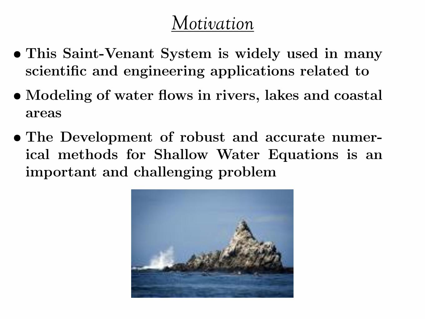
Motivation• This Saint-Venant System is widely used in many

scientific and engineering applications related to

• Modeling of water flows in rivers, lakes and coastalareas

• The Development of robust and accurate numer-ical methods for Shallow Water Equations is animportant and challenging problem

Motivation

!"""#

"""$

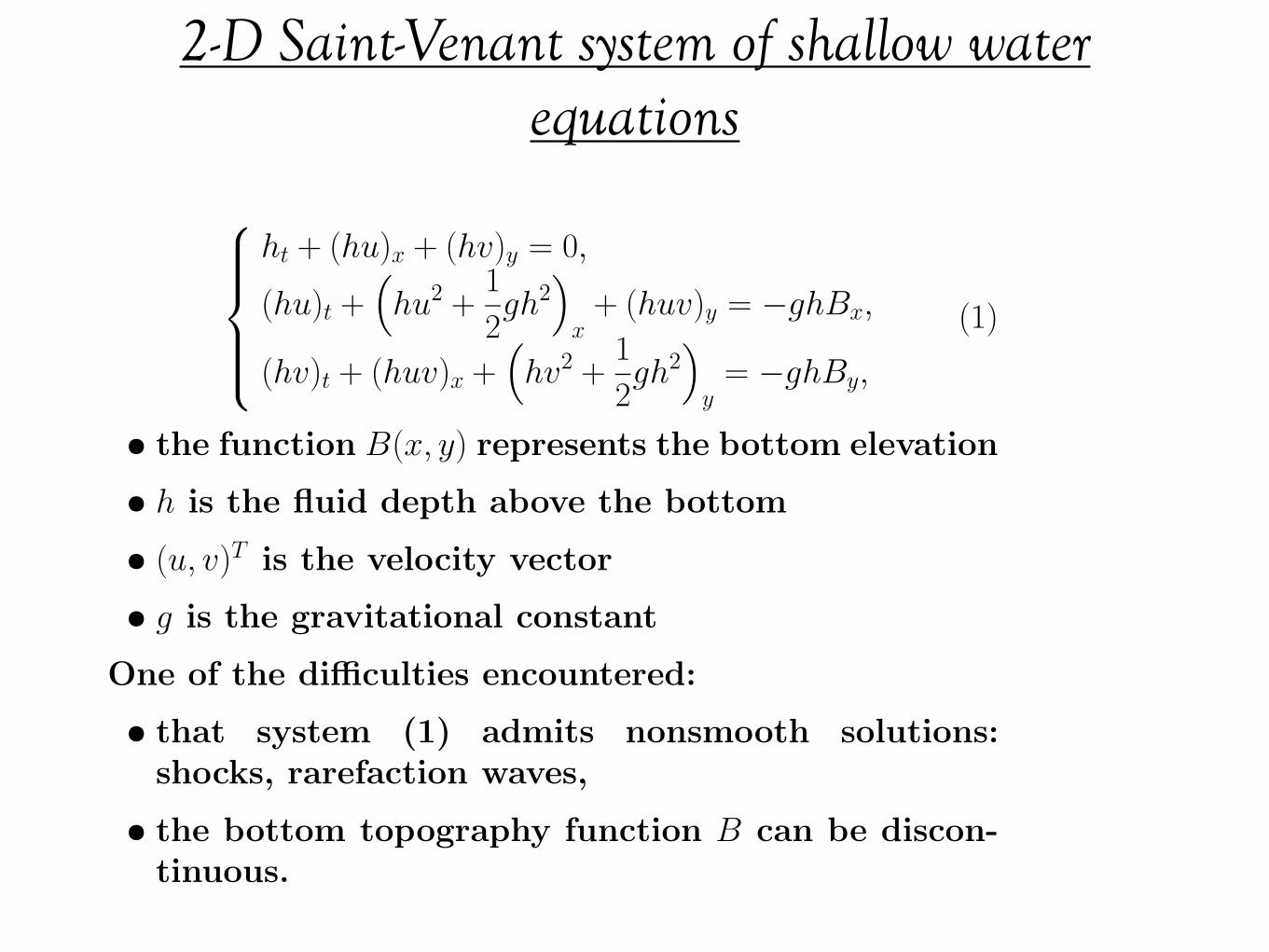
ht + (hu)x + (hv)y = 0,

(hu)t +%hu2 +

1

2gh2

&

x+ (huv)y = !ghBx,

(hv)t + (huv)x +%hv2 +

1

2gh2

&

y= !ghBy,

(1)

• the function B(x, y) represents the bottom elevation

• h is the fluid depth above the bottom

• (u, v)T is the velocity vector

• g is the gravitational constant

One of the di!culties encountered:

• that system (1) admits nonsmooth solutions:shocks, rarefaction waves,

• the bottom topography function B can be discon-tinuous.

Two-Dimensional (2-D) Saint-VenantSystem of Shallow Water Equations

2-D Saint-Venant system of shallow water equations

2-D Saint-Venant system of shallow water equations

A good numerical method for Saint-Venant System shouldhave at least two major properties, which are crucial for itsstability:

(i) The method should be well-balanced, that is, itshould exactly preserve the stationary steady-statesolutions h + B ! const, u ! v ! 0 (lake at reststates).This property diminishes the appearance of un-physical waves of magnitude proportional tothe grid size (the so-called “numerical storm”),which are normally present when computing quasisteady-states;

(ii) The method should be positivity preserving, thatis, the water depth h should be nonnegative at alltimes.This property ensures a robust performance of themethod on dry (h = 0) and almost dry (h " 0)states.

Semi-discrete central-upwind scheme

Central-Upwind schemes were developed for multidimensionalhyperbolic systems of conservation laws in 2000 ! 2007 byKurganov, Lin, Noelle, Petrova, Tadmor, ...

• Central-Upwind schemes are Godunov-type finite-volume projection-evolution methods:

• At each time level a solution is globally approxi-mated by a piecewise polynomial function,

• Which is then evolved to the new time level usingthe integral form of the conservation law system.

Semi-Discrete Central-Upwind Scheme

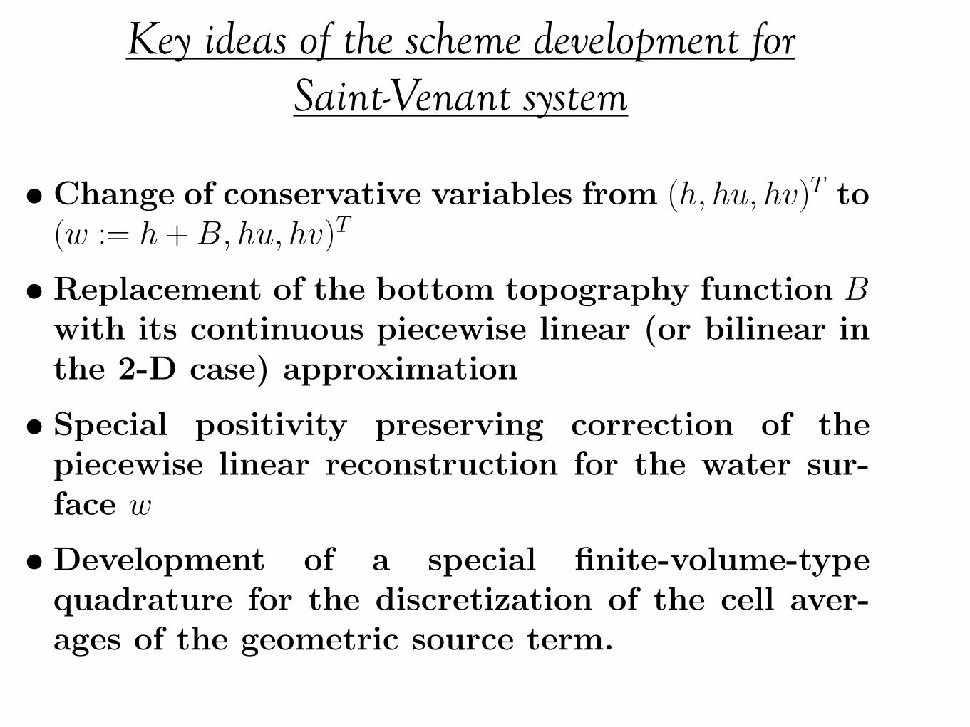
Key ideas of the scheme development for Saint-Venant system

• Change of conservative variables from (h, hu, hv)T to(w := h + B, hu, hv)T

• Replacement of the bottom topography function Bwith its continuous piecewise linear (or bilinear inthe 2-D case) approximation

• Special positivity preserving correction of thepiecewise linear reconstruction for the water sur-face w

• Development of a special finite-volume-typequadrature for the discretization of the cell aver-ages of the geometric source term.

Key ideas in the Development Scheme forSaint-Venant System

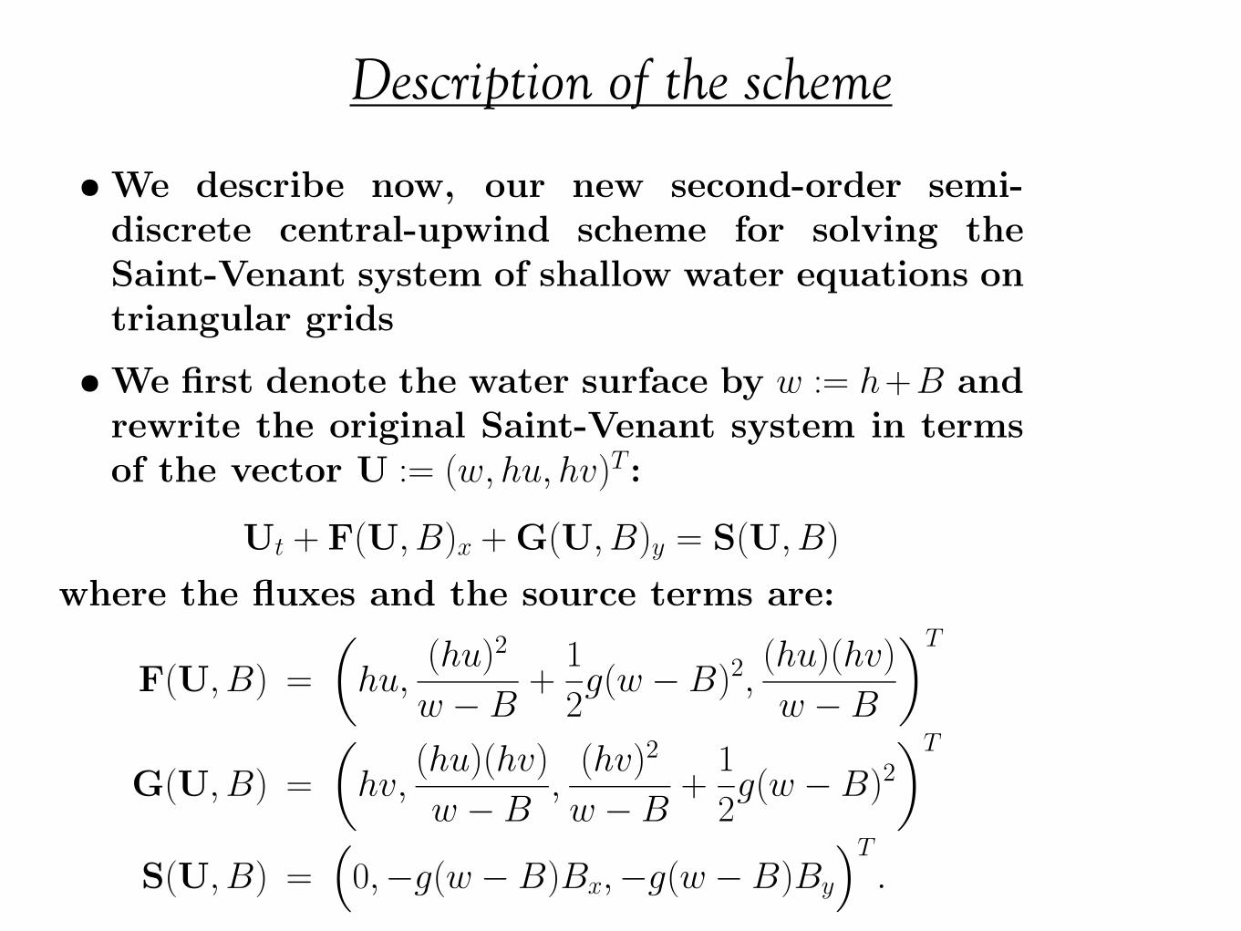
Description of the scheme

• We describe now, our new second-order semi-discrete central-upwind scheme for solving theSaint-Venant system of shallow water equations ontriangular grids

• We first denote the water surface by w := h+B andrewrite the original Saint-Venant system in termsof the vector U := (w, hu, hv)T :

Ut + F(U, B)x + G(U, B)y = S(U, B)

where the fluxes and the source terms are:

F(U, B) =

!hu,

(hu)2

w ! B+

1

2g(w ! B)2,

(hu)(hv)

w ! B

"T

G(U, B) =

!hv,

(hu)(hv)

w ! B,

(hv)2

w ! B+

1

2g(w ! B)2

"T

S(U, B) =#0,!g(w ! B)Bx,!g(w ! B)By

$T.

Description of the Scheme

Description of the scheme: notations

~

~

~

~

~

~

(x ,y )j j

(x ,y )j12 j12

(x ,y )j23 j23

(x ,y )j13 j13

Mj1

j3M

j2Mn

T

T

T

n

j1n

j2

T

j3j3

j

j2

j1

~

~

~

~

~

~

(x ,y )j j

(x ,y )j12 j12

(x ,y )j23 j23

(x ,y )j13 j13

Mj1

j3M

j2Mn

T

T

T

n

j1n

j2

T

j3j3

j

j2

j1

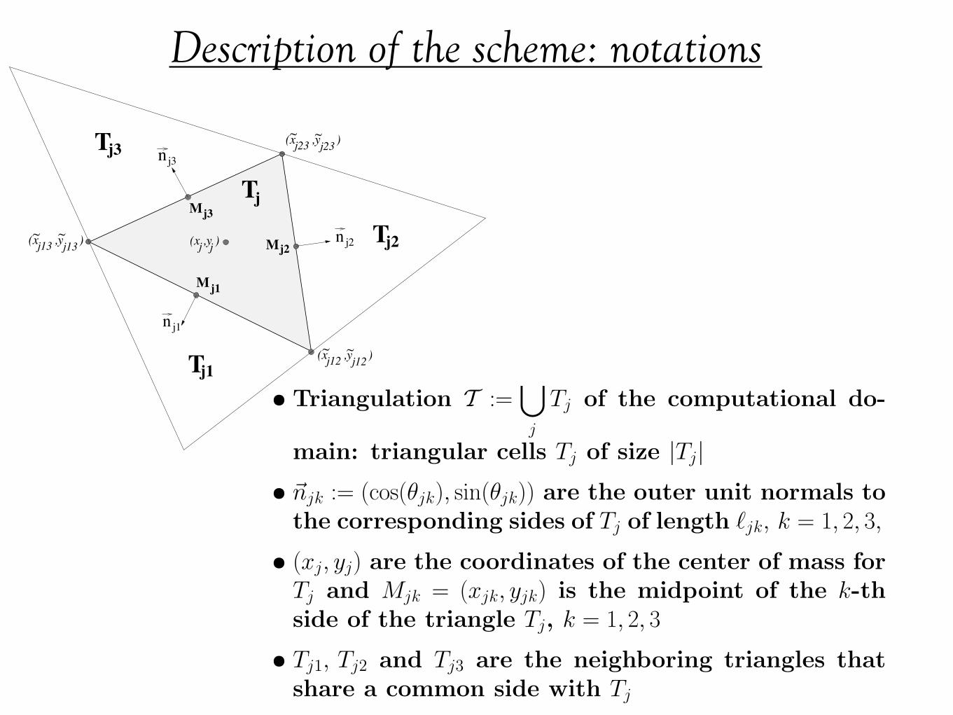
• Triangulation T :=!

j

Tj of the computational do-

main: triangular cells Tj of size |Tj|

• !njk := (cos("jk), sin("jk)) are the outer unit normals tothe corresponding sides of Tj of length #jk, k = 1, 2, 3,

• (xj, yj) are the coordinates of the center of mass forTj and Mjk = (xjk, yjk) is the midpoint of the k-thside of the triangle Tj, k = 1, 2, 3

• Tj1, Tj2 and Tj3 are the neighboring triangles thatshare a common side with Tj

Description of the Scheme: Notations

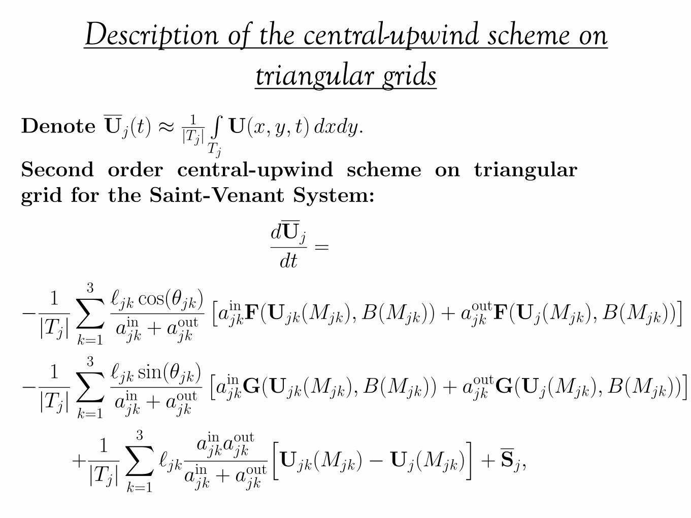
Description of the central-upwind scheme on triangular grids

Denote Uj(t) !1

|Tj|

!

Tj

U(x, y, t) dxdy.

Second order central-upwind scheme on triangulargrid for the Saint-Venant System:

dUj

dt=

"1

|Tj|

3"

k=1

!jk cos("jk)

ainjk + aout

jk

#ain

jkF(Ujk(Mjk), B(Mjk)) + aoutjk F(Uj(Mjk), B(Mjk))

$

"1

|Tj|

3"

k=1

!jk sin("jk)

ainjk + aout

jk

#ain

jkG(Ujk(Mjk), B(Mjk)) + aoutjk G(Uj(Mjk), B(Mjk))

$

+1

|Tj|

3"

k=1

!jk

ainjka

outjk

ainjk + aout

jk

%Ujk(Mjk) " Uj(Mjk)

&+ Sj,

Description of the Central-Upwind Schemeon Triangular Grids

Description of the central-upwind scheme on triangular grids

• Uj(Mjk) and Ujk(Mjk) are the corresponding valuesat Mjk of the piecewise linear reconstruction

U(x, y) := Uj +(Ux)j(x!xj)+ (Uy)j(y! yj), (x, y) " Tj

of U at time t

• The quantity Sj in the scheme is an appropriate dis-cretization of the cell averages of the source term

• The directional local speeds ainjk and aout

jk are definedby

ainjk(Mjk) = !min{!1[Vjk(Uj(Mjk))],!1[Vjk(Ujk(Mjk)], 0},

aoutjk (Mjk) = max{!3[Vjk(Uj(Mjk))],!3[Vjk(Ujk(Mjk)], 0},

where !1 [Vjk] # !2 [Vjk] # !3 [Vjk] are the eigenvaluesof the matrix Vjk = cos("jk)

#F#U + sin("jk)

#G#U.

• A fully discrete scheme is obtained by using a sta-ble ODE solver of an appropriate order

Description of the Central-Upwind Schemeon Triangular Grids

Calculation of the numerical derivatives of the ith component of U

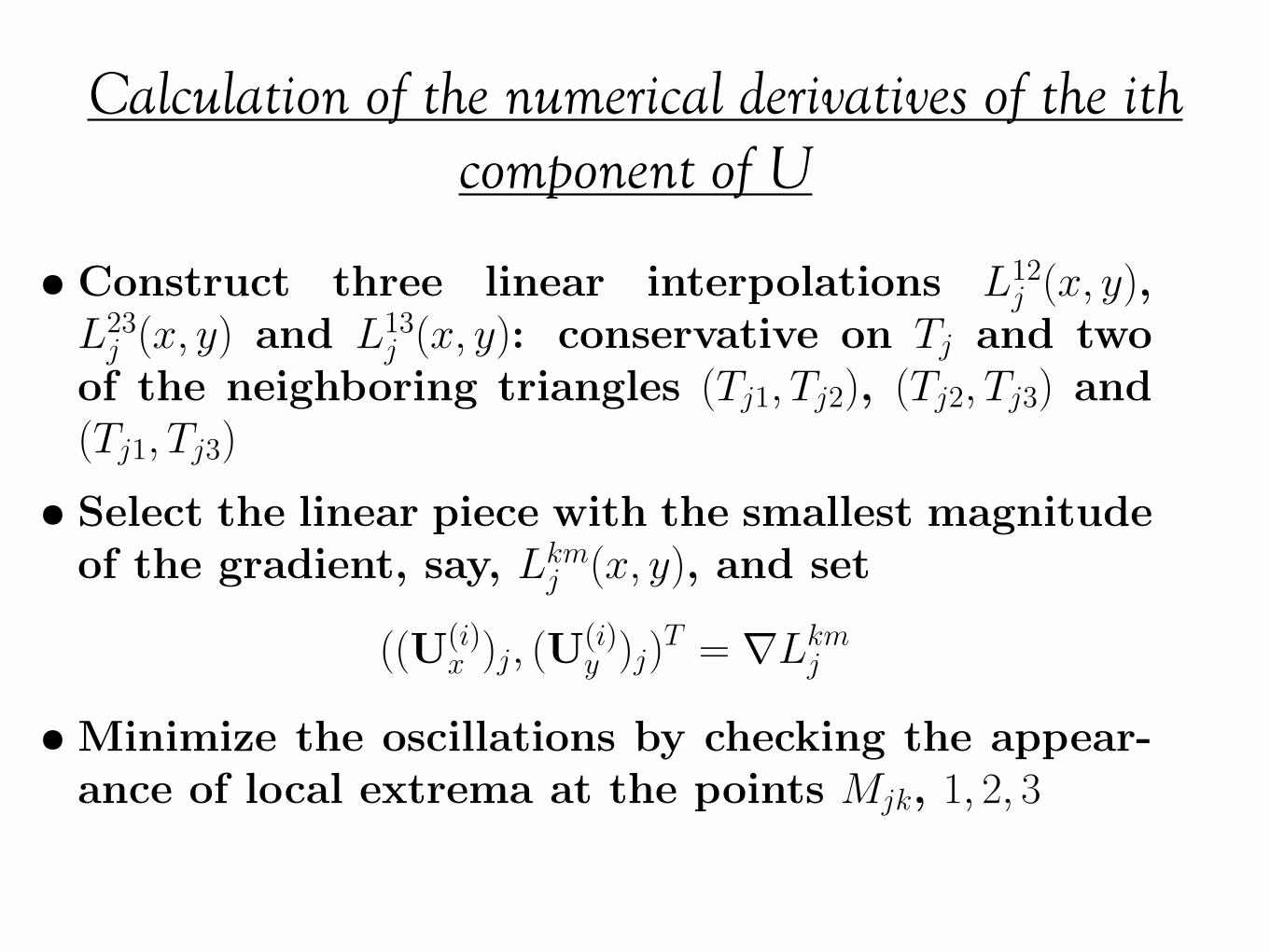
• Construct three linear interpolations L12j (x, y),

L23j (x, y) and L13

j (x, y): conservative on Tj and twoof the neighboring triangles (Tj1, Tj2), (Tj2, Tj3) and(Tj1, Tj3)

• Select the linear piece with the smallest magnitudeof the gradient, say, Lkm

j (x, y), and set

((U(i)x )j, (U

(i)y )j)

T = !Lkmj

• Minimize the oscillations by checking the appear-ance of local extrema at the points Mjk, 1, 2, 3

Calculation of the numerical derivatives ofthe ith component of U, (U(i)

x )j and (U(i)y )j

Piecewise linear approximation of the bottom

• Replace the bottom topography function B withits continuous piecewise linear approximation !B,which over each cell Tj is given by the formula:"""""""""

x ! xj12 y ! yj12!B(x, y) ! Bj12

xj23 ! xj12 yj23 ! yj12 Bj23 ! Bj12

xj13 ! xj12 yj13 ! yj12 Bj13 ! Bj12

"""""""""

= 0, (x, y) " Tj.

• Bj! are the values of !B at the vertices (xj!, yj!), ! =12, 23, 13, of the cell Tj

Piecewise Linear Approximation of theBottom

• Bj! := 12(max"2+#2=1 limh,$!0 B(xj! + h", yj! + $#) +

min"2+#2=1 limh,$!0 B(xj! + h", yj! + $#)),

• If the function B is continuous at (xj!, yj!): Bj! =B(xj!, yj!)

• Denote by Bjk the value of the continuous piecewiselinear reconstruction at Mjk, Bjk := !B(Mjk),and by Bj := !B(xj, yj) the value of the reconstructionat the center of mass (xj, yj) of Tj,

• Notice that, in general, Bjk "= B(Mjk) and

Bj =1

|Tj|

"

Tj

!B(x, y) dxdy,

• One can easily show that

Bj =1

3(Bj1 + Bj2 + Bj3) =

1

3(Bj12 + Bj23 + Bj13) .

Positivity preserving reconstruction for w

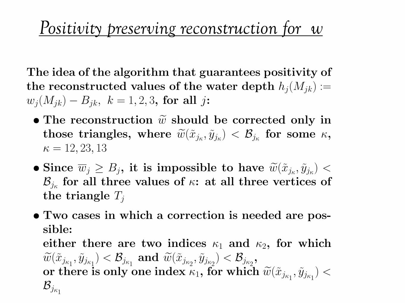
The idea of the algorithm that guarantees positivity ofthe reconstructed values of the water depth hj(Mjk) :=wj(Mjk) ! Bjk, k = 1, 2, 3, for all j:

• The reconstruction !w should be corrected only inthose triangles, where !w(xj!, yj!) < Bj! for some !,! = 12, 23, 13

• Since wj " Bj, it is impossible to have !w(xj!, yj!) <Bj! for all three values of !: at all three vertices ofthe triangle Tj

• Two cases in which a correction is needed are pos-sible:either there are two indices !1 and !2, for which!w(xj!1

, yj!1) < Bj!1

and !w(xj!2, yj!2

) < Bj!2,

or there is only one index !1, for which !w(xj!1, yj!1

) <Bj!1

Positivity Preserving Reconstruction for w

Well-balanced discretization of the source term

• The well-balanced property of the scheme is guar-anteed if the discretized cell average of the sourceterm, Sj, exactly balances the numerical fluxes

• The desired quadrature for the source term thatwill preserve stationary steady states (Ujk(Mjk) !Uj(Mjk) ! (C, 0, 0)T , "j, k) is given by:

S(2)j =

g

2|Tj|

3!

k=1

!jk(wj(Mjk) # Bjk)2 cos("jk) # g(wx)j(wj # Bj)

S(3)j =

g

2|Tj|

3!

k=1

!jk(wj(Mjk) # Bjk)2 sin("jk) # g(wy)j(wj # Bj)

Well-Balanced Discretization of the SourceTerm

Main theorem: positivity property of the new scheme

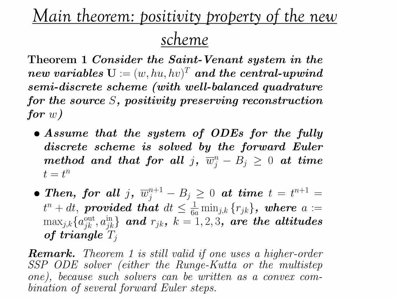
Theorem 1 Consider the Saint-Venant system in thenew variables U := (w, hu, hv)T and the central-upwindsemi-discrete scheme (with well-balanced quadraturefor the source S, positivity preserving reconstructionfor w)

• Assume that the system of ODEs for the fullydiscrete scheme is solved by the forward Eulermethod and that for all j, wn

j ! Bj " 0 at timet = tn

• Then, for all j, wn+1j ! Bj " 0 at time t = tn+1 =

tn + dt, provided that dt # 16a minj,k {rjk}, where a :=

maxj,k{aoutjk , ain

jk} and rjk, k = 1, 2, 3, are the altitudesof triangle Tj

Remark. Theorem 1 is still valid if one uses a higher-orderSSP ODE solver (either the Runge-Kutta or the multistepone), because such solvers can be written as a convex com-bination of several forward Euler steps.

Positivity Preserving Reconstruction for w

Accuracy test

The scheme is applied to the Saint-Venant system sub-ject to the following initial data and the bottom to-pography:

w(x, y, 0) = 1, u(x, y, 0) = 0.3,

B(x, y) = 0.5 exp(!25(x ! 1)2 ! 50(y ! 0.5)2).

• For a reference solution, we solve this problem withour method on a 2 " 400 " 400 triangular grid

• By t = 0.07 the solution converges to the steadystate

Accuracy Test

Accuracy test

• w component of the reference solution ofthe IVP on a 2 ! 400 ! 400 grid: the 3-D view (left) and the contour plot (right).

0 0.5 1 1.5 20

0.2

0.4

0.6

0.8

1

• L1- and L"-errors and numerical orders of accuracy.

Number of cells L1-error Order L"-error Order2 ! 50 ! 50 6.59e-04 – 8.02e-03 –

2 ! 100 ! 100 2.87e-04 1.20 3.59e-03 1.162 ! 200 ! 200 1.00e-04 1.52 1.21e-03 1.57

Accuracy Test

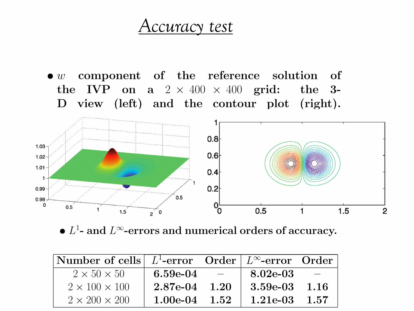
• w component of the reference solution ofthe IVP on a 2 ! 400 ! 400 grid: the 3-D view (left) and the contour plot (right).

0 0.5 1 1.5 20

0.2

0.4

0.6

0.8

1

• L1- and L"-errors and numerical orders of accuracy.

Number of cells L1-error Order L"-error Order2 ! 50 ! 50 6.59e-04 – 8.02e-03 –

2 ! 100 ! 100 2.87e-04 1.20 3.59e-03 1.162 ! 200 ! 200 1.00e-04 1.52 1.21e-03 1.57

Accuracy Test

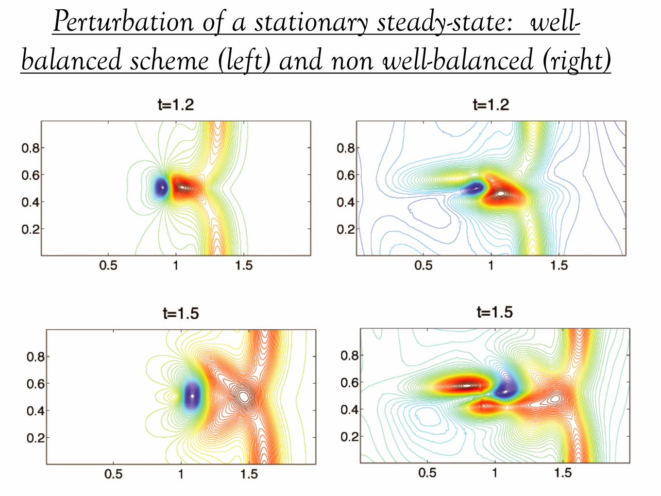
Small perturbation of a stationary steady-state solution

• Solve the initial value problem (IVP) proposed byR.Leveque.

• The computational domain is [0, 2] ! [0, 1] and thebottom consists of an elliptical shaped hump:

B(x, y) = 0.8 exp("5(x " 0.9)2 " 50(y " 0.5)2).

• Initially, the water is at rest and its surface is flateverywhere except for 0.05 < x < 0.15:

w(x, y, 0) =

!1 + !, 0.05 < x < 0.15,1, otherwise,

u(x, y, 0) # v(x, y, 0) # 0,

where the perturbation height is ! = 10"4

Small Perturbation of a StationarySteady-State Solution

Perturbation of a stationary steady-state: well-balanced scheme (left) and non well-balanced (right)

Perturbation of a stationary steady-state: well-balanced scheme (left) and non well-balanced (right)

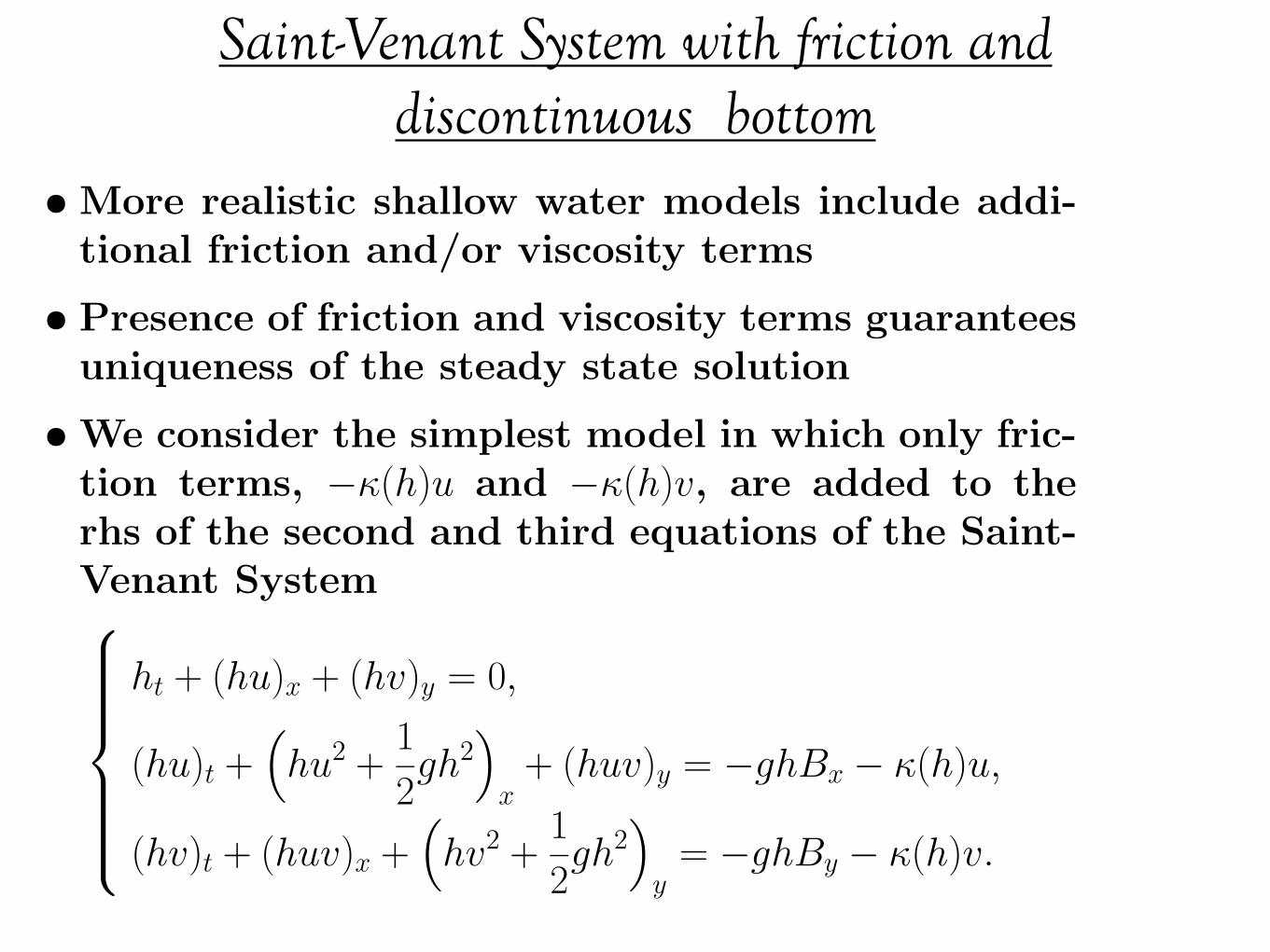
Saint-Venant System with friction and discontinuous bottom

• More realistic shallow water models include addi-tional friction and/or viscosity terms

• Presence of friction and viscosity terms guaranteesuniqueness of the steady state solution

• We consider the simplest model in which only fric-tion terms, !!(h)u and !!(h)v, are added to therhs of the second and third equations of the Saint-Venant System!"""""#

"""""$

ht + (hu)x + (hv)y = 0,

(hu)t +%hu2 +

1

2gh2

&

x+ (huv)y = !ghBx ! !(h)u,

(hv)t + (huv)x +%hv2 +

1

2gh2

&

y= !ghBy ! !(h)v.

Saint-Venant System with friction and discontinuous bottom

• We numerically solve the shallow water model withfriction term on the domain [!0.25, 1.75] " [!0.5, 0.5]

• We assume that the friction coe!cient is

!(h) = 0.001(1 + 10h)!1

• The bottom topography function has a discontinu-ity along the vertical line x = 1 and it mimics amountain river valley

!!"# ! !"# $ $"# %!!"#

!!"#

!

$

%

&

'

#

(

)

*

Saint-Venant System with friction and discontinuous bottom: description of the initial and boundary

conditions• We implement reflecting (solid wall) boundary con-

ditions at all boundaries

• Our initial data correspond to the situation whenthe second of the three dams, initially located atthe vertical linesx = !0.25 (the left boundary of the computational do-main), x = 0, and x = 1.75 (the right boundary of thecomputational domain),breaks down at time t = 0, and the water propa-gates into the initially dry area x > 0, and a “lake atrest” steady state is achieved after a certain periodof time

• We plot 1-D slices of the numerical solution alongthe y = 0 line

• Plots clearly show the dynamics of the fluid flowas it moves from the region x < 0 into the initiallydry area x > 0 and gradually settles down into a“lake at rest” steady state

• This state includes dry areas and therefore its com-putation requires a method that is both well-balancedand positivity preserving on the entire computational do-main

• We plot 1-D slices of the numerical solution alongthe y = 0 line

• Plots clearly show the dynamics of the fluid flowas it moves from the region x < 0 into the initiallydry area x > 0 and gradually settles down into a“lake at rest” steady state

• This state includes dry areas and therefore its com-putation requires a method that is both well-balancedand positivity preserving on the entire computational do-main

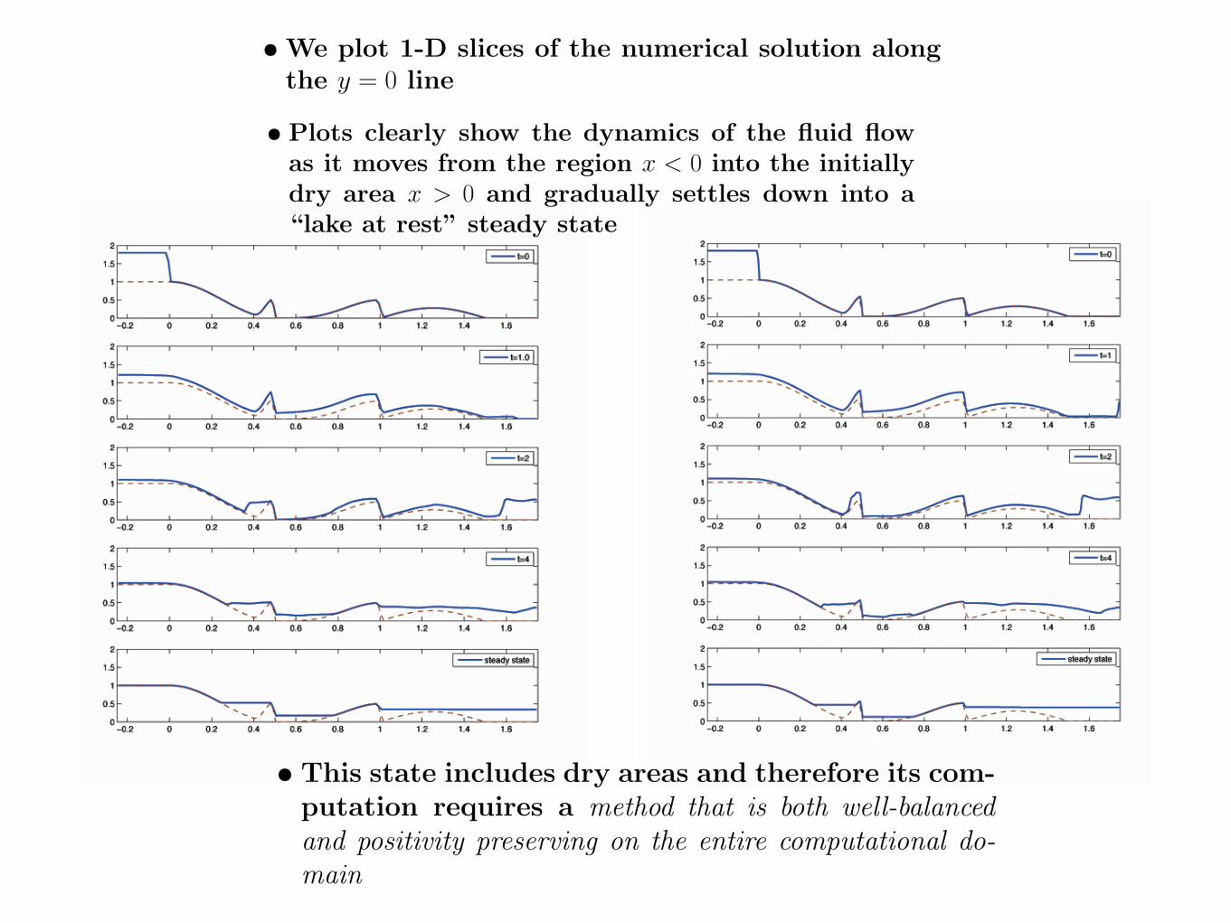
• We plot 1-D slices of the numerical solution alongthe y = 0 line

• Plots clearly show the dynamics of the fluid flowas it moves from the region x < 0 into the initiallydry area x > 0 and gradually settles down into a“lake at rest” steady state

• This state includes dry areas and therefore its com-putation requires a method that is both well-balancedand positivity preserving on the entire computational do-main

Flow in converging-diverging channel

• The exact geometry of each channel is determinedby its breadth, which is equal to 2yb(x), where

yb(x) =

!0.5 ! 0.5(1 ! d) cos2(!(x ! 1.5)), |x ! 1.5| " 0.5,0.5, otherwise,

• d = 0.6 is the minimum channel breadth

d

Flow in Converging-Diverging Channel

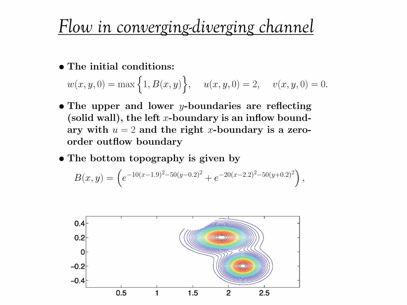
Flow in converging-diverging channel

• The initial conditions:

w(x, y, 0) = max!

1, B(x, y)"

, u(x, y, 0) = 2, v(x, y, 0) = 0.

• The upper and lower y-boundaries are reflecting(solid wall), the left x-boundary is an inflow bound-ary with u = 2 and the right x-boundary is a zero-order outflow boundary

• The bottom topography is given by

B(x, y) =#e!10(x!1.9)2!50(y!0.2)2 + e!20(x!2.2)2!50(y+0.2)2

$,

0.5 1 1.5 2 2.5

!0.4

!0.2

0

0.2

0.4

Flow in Converging-Diverging Channel

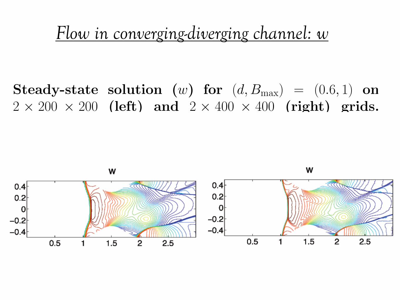
Flow in converging-diverging channel: w

Steady-state solution (w) for (d,Bmax) = (0.6, 1) on2 ! 200 ! 200 (left) and 2 ! 400 ! 400 (right) grids.

w

0.5 1 1.5 2 2.5

!0.4

!0.2

0

0.2

0.4

w

0.5 1 1.5 2 2.5

!0.4

!0.2

0

0.2

0.4

Flow in Converging-Diverging Channel: wcomponent

Conclusions/Difficulties

• We developed a simple central-upwind scheme forthe Saint-Venant system on triangular grids

• We proved that the scheme both preserves station-ary steady states (lake at rest) and guarantees thepositivity of the computed fluid depth

• It can be applied to models with discontinuous bot-tom topography and irregular channel widths

• Method is sensitive to the accuracy of the bound-ary representation

• S. Bryson, Y. Epshteyn, A. Kurganov andG. Petrova, Well-Balanced Positivity PreservingCentral-Upwind Scheme on Triangular Grids forthe Saint-Venant System, to appear, ESAIM:M2AN 2010.

Conclusions/Di!culties