WEBIRA-ComparativeAnalysisofWeightBalancingMethoddspace.vgtu.lt/bitstream/1/3730/1/WEBIRA -...

INTERNATIONAL JOURNAL OF COMPUTERS COMMUNICATIONS & CONTROLISSN 1841-9836, 12(2):238-253, April 2017.

WEBIRA - Comparative Analysis of Weight Balancing Method

A. Krylovas, N. Kosareva, E.K. Zavadskas

Aleksandras Krylovas, Natalja Kosareva*,Edmundas Kazimieras ZavadskasVilnius Gediminas Technical UniversitySauletekio al. 11, LT-10223 Vilnius, [email protected], [email protected],[email protected]*Corresponding author: [email protected]

Abstract: The attributes weight establishing problem is one of the most importantMCDM tasks. This study summarizes weight determining approach which is calledWEBIRA (WEight Balancing Indicator Ranks Accordance). This method requiresto solve complicated optimization problem and its application is possible by carryingout non trivial calculations. The efficiency of WEBIRA and other MCDM methods –SAW (Simple Additive Weighting) and EMDCW (Entropy Method for Determiningthe Criterion Weight) compared for 4 different data normalization methods. The re-sults of the study revealed that more sophisticated WEBIRA method is significantlyefficient for all considered numbers of alternatives. Efficiency of all methods decreaseswith increasing number of alternatives, but WEBIRA is still applicable, while appli-cation of other methods is impossible as the number of alternatives is greater than11. WEBIRA is the least affected by the data normalization, while EMDCW is themost affected method.Keywords: WEBIRA, SAW, EMDCW, multi-attribute decision making (MADM),entropy, KEMIRA.

1 Introduction

From the large diversity of MCDM methods some are very simple to use methods, andthe other – complex, requiring more effort and computing resources. This article analyses theattributes weighting task, which is solved by different methods. One of the main and well knownmultiple criteria decision making (MCDM) methods is calculation of weighted averages of thethe performance values of alternatives evaluated in terms of attributes (criteria):

S(j) (W,R) =n∑i=1

wir(j)i , j = 1, 2, . . . ,m, (1)

here W = (w1, w2, . . . , wn), 0 6 wi 6 1,n∑i=1

wi = 1 is vector of weights, n – number of attributes,

R =

r

(1)1 r

(1)2 . . . r

(1)n

r(2)1 r

(2)2 . . . r

(2)n

. . . . . . . . . . . .

r(m)1 r

(m)2 . . . r

(m)n

– matrix of alternatives j ∈ {1, 2, . . . ,m} estimates, which

elements 0 6 r(j)i 6 1 are obtained by certain measurements or expert assessments applying

different calculation procedures, which are usually referred to as normalization methods (see[1, 2]). For example, in this article maximum method (Max), sums method (Sum), minmaxmethod (MinMax) and vector normalization (Vctr) will be used.

The mentioned MCDM method is known as WSM (Weighted Sum Model). It was noticedby Churchman in 1954 [3] that "course of action that maximizes the expected total weighted

Copyright © 2006-2017 by CCC Publications

WEBIRA - Comparative Analysis of Weight Balancing Method 239

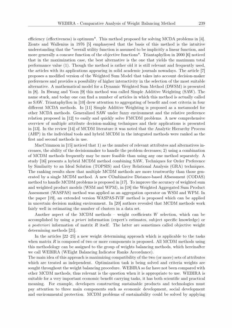
efficiency (effectiveness) is optimum". This method proposed for solving MCDA problems in [4].Zionts and Wallenius in 1976 [5] emphasysed that the basis of this method is the intuitiveunderstanding that the "overall utility function is assumed to be implicitly a linear function, andmore generally a concave function of the objective functions". Triantaphyllou in 2000 [6] noticedthat in the maximization case, the best alternative is the one that yields the maximum totalperformance value (1). Though the method is rather old it is still relevant and frequently used,the articles with its applications appearing in solid academic journals nowadays. The article [7]proposes a modified version of the Weighted Sum Model that takes into account decision-makerpreferences and provides a possibility of higher interactivity in the selection of the most suitablealternative. A mathematical model for a Dynamic Weighted Sum Method (DWSM) is presentedin [8]. In Hwang and Yoon [9] this method was called Simple Additive Weighting (SAW). Thename stuck, and today one can find a number of articles in which this method is actually calledas SAW. Triantaphyllou in [10] drew attention to aggregating of benefit and cost criteria in fourdifferent MCDA methods. In [11] Simple Additive Weighting is proposed as a metamodel forother MCDA methods. Generalized SAW under fuzzy environment and the relative preferencerelation proposed in [12] to easily and quickly solve FMCDM problems. A new comprehensiveoverview of multiple attribute decision-making techniques and their applications is presentedin [13]. In the review [14] of MCDM literature it was noted that the Analytic Hierarchy Process(AHP) in the individual tools and hybrid MCDM in the integrated methods were ranked as thefirst and second methods in use.

MacCrimmon in [15] noticed that 1) as the number of relevant attributes and alternatives in-creases, the ability of the decisionmaker to handle the problem decreases; 2) using a combinationof MCDM methods frequently may be more feasible than using any one method separately. Astudy [16] presents a hybrid MCDM method combining SAW, Techniques for Order Preferenceby Similarity to an Ideal Solution (TOPSIS) and Grey Relational Analysis (GRA) techniques.The ranking results show that multiple MCDM methods are more trustworthy than those gen-erated by a single MCDM method. A new COmbinative Distance-based ASsessment (CODAS)method to handle MCDM problems is proposed in [17]. To improve the accuracy of weighted sumand weighted product models (WSM and WPM), in [18] the Weighted Aggregated Sum ProductAssessment (WASPAS) method was applied as an aggregation operator on WSM and WPM. Inthe paper [19], an extended version WASPAS-IVIF method is proposed which can be appliedin uncertain decision making environment. In [20] authors revealed that MCDM methods workfairly well in estimating the number of clusters in a data set.

Another aspect of the MCDM methods – weight coefficients W selection, which can beaccomplished by using a priori information (expert’s estimates, subject specific knowledge) ora posteriori information of matrix R itself. The latter are sometimes called objective weightdetermining methods [21].

In the articles [22–25] a new weight determining approach which is applicable to the taskswhen matrix R is composed of two or more components is proposed. All MCDM methods usingthis methodology can be assigned to the group of weights balancing methods, which hereinafterwe call WEBIRA (WEight Balancing Indicator Ranks Accordance).The main idea of this approach is maximizing compatibility of the two (or more) sets of attributeswhich are treated as independent. Optimization task is being solved and criteria weights aresought throughout the weight balancing procedure. WEBIRA so far have not been compared withother MCDM methods, thus relevant is the question when it is appropriate to use. WEBIRA issuitable for a very important economic benefit carrying tasks, it has both scientific and practicalmeaning. For example, developers constructing sustainable products and technologies mustpay attention to three main components such as economic development, social developmentand environmental protection. MCDM problems of sustainability could be solved by applying

240 A. Krylovas, N. Kosareva, E.K. Zavadskas

WEBIRA for 3 sets of attributes – economic, social and environmental components of sustainabledevelopment.

A major criticism of MADM is that different techniques may yield different results whenapplied to the same problem. It does not exist multiple criteria evaluation method which is"best under any circumstances". Therefore the comparative analysis of various MCDM methodsdetermining which method is best for a particular case is relevant and important task. The per-formance of eight methods: ELimination and Choice Expressing REality (ELECTRE), TOPSIS,Multiplicative Exponential Weighting (MEW), SAW, and four versions of AHP investigated insimulation experiment in [26]. Simulation parameters are the number of alternatives, criteriaand their distribution. In general, all AHP versions behave similarly and closer to SAW thanthe other methods. ELECTRE is the least similar to SAW. The following performance order ofmethods was established: SAW and MEW (best), followed by TOPSIS, AHPs and ELECTRE.The comparative analysis of MCDA methods SAW and COPRAS (Complex Proportional As-sessment) describing their common and diverse characteristics is proposed in [27]. The paper [28]presents an empirical application and comparison of six different MCDM approaches (betweenthem WSM, AHP, TOPSIS, COPRAS) for the purpose of assessing sustainable housing afford-ability. TOPSIS, SAW, and Mixed (Rank Average) for decision-making as well as AHP andEntropy for obtaining the weights of attributes have been compared in [29]. Mixed method ascompared to TOPSIS and SAW is the preferred technique, moreover, AHP is more acceptablethan Entropy for weighting. The comprehensive study [30] carried out the comparative analy-sis among well-known and widely-used methods WPM, WSM, TOPSIS, AHP, PROMETHEE,ELECTRE, when applied to the reference problem of the selection of wind turbine supportstructures for a given deployment location. The outcomes of this research highlight that moresophisticated methods, such as TOPSIS and Preference Ranking Organization METHod forEnrichment Evaluation (PROMETHEE), better predict the optimum design alternative.

WEBIRA method requires to solve complicated optimization task and therefore it relatesto executing non trivial computer calculations. Naturally, the question arises as to when itwould appear reasonable to apply WEBIRA, and when – the less sophisticated approaches. Inthis article Monte Carlo-type experiments are performed and WEBIRA is compared with twosimple objective weight determining methods: AVRG – the simple arithmetic average, i. e. theweighted sum with equal weights and the Entropy Method for Determining the Criterion Weight(EMDCW) described in [21]. The Shannon entropy method [31] is one of the most famousapproach for determining the objective attribute weights. Entropy measures the uncertaintyassociated with a random variable, i.e. the expected value of the information transmitted tothe decision maker. The authors of the paper [21] have combined the best features of theentropy method and the CILOS (the Criterion Impact Loss) approach to obtain a new method –Integrated Determination of Objective CRIteria Weights, or (IDOCRIW). In [32] three methodshave been used for estimating criteria weights: Entropy, CILOS and IDOCRIW, while for theselection of priority well-known and widely used MCDM methods SAW, TOPSIS and COPRAShave been used in MCDM analysis of operating of rotor systems with tilting pad bearings.

Another problem the article dealt with – the comparative analysis of efficiency of some datanormalization methods. A state-of-the-art survey on the influence of normalization techniques inranking is proposed in [33]. Thirty-one methods were identified, classified and evaluated for use inmaterials selection problems. Review of normalization methods used in construction engineeringand management, and their applications presented in [34].

The article is organized as follows. In Chapter 2 the algorithm of solving the optimizationproblem and the case study of its application is proposed. In Chapter 3 random matrices gen-erating scheme is described. In Chapter 4 the transformation formulas for matrix of estimatesproposed. Chapter 5 describes the process of numerical experiments and methods of efficiency


comparison. Chapter 6 describes the statistical analysis of the results of numerical experiments,summarizes and proposes recommendations for application of various MCDM methods and nor-malizing procedures.

2 Algorithm of WEBIRA method

Suppose, that matrix R is composed of two componentsR = (P |Q), P =

(p

(j)i

)m×np

, Q =(q

(j)i

)m×nq

, np + nq = n.

Two weighted sums are calculated

S(j)P =

np∑i=1

wPip(j)i , S

(j)Q =

nq∑i=1

wQiq(j)i , j = 1, 2, . . . ,m. (2)

Coefficients WP =(wp1, wp2, . . . , wpnp

), WQ =

(wq1, wq2, . . . , wqnq

)satisfy monotonicity condi-

tions:1 > wp1 > wp2 > · · · > wpnp > 0, 1 > wq1 > wq2 > · · · > wqnq > 0. (3)

Inequalities (3) are set from expert estimates, when k experts line up attributes pie, qie accordingto their importance:

pi1e � pi2e � · · · � pinpe, qi1e � · · · � qi2e � qinq e, e = 1, 2, . . . , k. (4)

When we have a priori information about experts evaluations (4), inequalities (3) could beobtained by different methods. In the article [22] Kemeny median has been adapted for thispurpose and the name KEMIRA (KEmeny Median Indicator Ranks Accordance) proposed forthe method. In the articles [23–25] inequalities (3) were set by calculating entropy values or byapplication of voting theory methods. As the inequalities (3) indicating the weight preferences areestablished, all of the mentioned methods can be assigned to the objective weight determining,because there is not need of further information to set the weights of the attributes. We considerthe task when inequalities (3) already established and the weights WP , WQ determining task isbeing solved. The task is formulated as minimization of a certain distance or measure:

s (WP ,WQ) = minWP ,WQ

√√√√ 1

m

m∑j=1

(S

(j)P − S

(j)Q

)2, (5)

where the weights WP , WQ are satisfying the inequalities (3). So, all the mentioned MCDMmethods [22–25] can be assigned to the group of weight balancing methods, which we call WE-BIRA.

In this article we analyze only the benefit type attributes, i.e. whose higher value is better.When optimization task (5),(3) is already solved, the ranks can be assigned to the alternativesj ∈ {1, 2, . . . ,m} depending on the size of the weighted sums S(j)

P and S(j)Q . Suppose that jP1 ,

jP2 , . . ., jPm, jQ1 , jQ2 , . . ., jQm are such numbers of alternatives that the weighted sums (2) are

satisfying the inequalities:

SjP1P > S

jP2P > · · · > S

jPmP , S

jQ1Q > S

jQ2Q > · · · > Sj

Qm

Q . (6)

Denote a set of the best k alternatives according to the first np attributes APk = {jP1 , jP2 , . . . , jPk },according to the last nq attributes – A

Qk = {jQ1 , jQ2 , . . . , jQk } and their intersection A = APk ∩A

Qk .


The meaning of the sets APk and AQk is selecting the best k alternatives according to the attributesP and Q respectively while the meaning of the set A – the best alternatives according to the bothattributes. The purpose of WEBIRA method is to balance weights so that a number of elements|A| of the set A would be not less than the certain number. So, it is required to find a sufficientnumber of the best alternatives according to both attributes P and Q. In the articles [22–25]the minimizing tasks (5),(3) have been solved together with max |A| under various parameterk values of the sets APk and AQk . In the current article we limit ourselves to the case k = 1and require A 6= ∅, i. e. we will search the only one the best alternative according to the bothattributes P and Q.

This additional condition can be formulated as follows:

S(jP0 )P = max

j=1,2,...,m{S(j)

P }, S(jQ0 )Q = max

j=1,2,...,m{S(j)

Q }, jP0 = jQ0 . (7)

Algorithm of solving the problem (5),(3),(7) is as follows.

1. By random re-selection among weights WP , WQ satisfying conditions (3) the weights sat-isfying an additional condition (7) are being searched.

2. If the weights W 0P , W

0Q were not found after iter0 iterations, algorithm is finishing work

and it is concluded that the weights can not be determined.

3. If the weights W 0P , W

0Q are set, the loss value (5) is fixed as s0, directions ∆WP , ∆WQ

are selected at random and the new weights W 1P = W 0

P + h∆WP , W 1Q = W 0

Q + h∆WQ

calculated, here h is the predetermined value.

4. The correction of weights W 1P , W

1Q is performed as follows W → W :

W = (w1, w2, . . . , wn), wi =

1, if wi > 1,0, if wi 6 0,wi, else,

then the weights are normalized wi = win∑i=1

wi

.

5. Checking whether the new weights W 1P , W

1Q satisfy the condition (7). If they satisfy and

the number of iterations does not exceed the established limit iter1 the algorithm movesto the Step 7.

6. If the number of iterations exceeds the established limit iter1, algorithm finishes its workwith the determined weights W 0

P , W0Q.

7. The loss value (5) is calculated s1(W 1P ,W

1Q

). If s1 6 s0, we substitute W 0

P = W 1P ,

W 0Q = W 1

Q, s0 = s1 and then the new weights W 1

P , W1Q are calculated with the same

directions ∆WP , ∆WQ. Go to the weight correction procedure to the Step 4.

8. If s1 > s0, the directions ∆WP , ∆WQ are changed randomly, i. e. go to the Step 3 ofalgorithm.


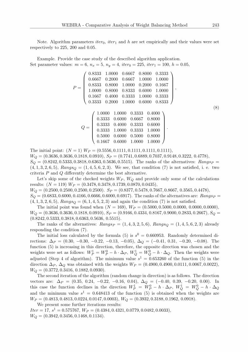
Note. Algorithm parameters iter0, iter1 and h are set empirically and their values were setrespectively to 225, 200 and 0.05.

Example. Provide the case study of the described algorithm application.Set parameter values: m = 6, nx = 5, ny = 4, iter0 = 225, iter1 = 100, h = 0.05,

P =

0.8333 1.0000 0.6667 0.8000 0.33330.6667 0.2000 0.6667 1.0000 1.00000.8333 0.8000 1.0000 0.2000 0.16671.0000 0.8000 0.8333 0.6000 1.00000.1667 0.4000 0.3333 1.0000 0.33330.3333 0.2000 1.0000 0.6000 0.8333

,

Q =

1.0000 1.0000 0.3333 0.40000.3333 0.6000 0.6667 0.80000.3333 0.4000 0.3333 0.60000.3333 1.0000 0.3333 1.00000.5000 0.6000 0.5000 0.80000.1667 0.6000 1.0000 1.0000

.

(8)

The initial point: (N = 1) WP = (0.5556, 0.1111, 0.1111, 0.1111, 0.1111),WQ = (0.3636, 0.3636, 0.1818, 0.0910), SP = (0.7741, 0.6889, 0.7037, 0.9148, 0.3222, 0.4778),SQ = (0.8242, 0.5333, 0.3818, 0.6363, 0.5636, 0.5515). The ranks of the alternatives: RangsP =(4, 1, 3, 2, 6, 5), RangsQ = (1, 4, 5, 6, 2, 3). We see, that condition (7) is not satisfied, i. e. twocriteria P and Q differently determine the best alternative.

Let’s skip some of the checked weights WP , WQ and provide only some of the calculationsresults: (N = 119) WP = (0.3478, 0.3478, 0.1739, 0.0870, 0.0435),WQ = (0.2500, 0.2500, 0.2500, 0.2500). SP = (0.8377, 0.5478, 0.7667, 0.8667, 0.3565, 0.4478),SQ = (0.6833, 0.6000, 0.4166, 0.6666, 0.6000, 0.6917). The ranks of the alternatives are: RangsP =(4, 1, 3, 2, 6, 5), RangsQ = (6, 1, 4, 5, 2, 3) and again the condition (7) is not satisfied.

The initial point was found when (N = 169), WP = (0.5000, 0.5000, 0.0000, 0.0000, 0.0000),WQ = (0.3636, 0.3636, 0.1818, 0.0910), SP = (0.9166, 0.4334, 0.8167, 0.9000, 0.2833, 0.2667), SQ =(0.8242, 0.5333, 0.3818, 0.6363, 0.5636, 0.5515).

The ranks of the alternatives: RangsP = (1, 4, 3, 2, 5, 6), RangsQ = (1, 4, 5, 6, 2, 3) alreadyresponding the condition (7).

The initial loss calculated by the formula (5) is s0 = 0.660953. Randomly determined di-rections: ∆P = (0.30, −0.30, −0.22, −0.13, −0.05), ∆Q = (−0.41, 0.31, −0.20, −0.08). Thefunction (5) is increasing in this direction, therefore, the opposite direction was chosen and theweights were set as follows: W 1

P = W 0P − h · ∆P , W 1

Q = W 0Q − h · ∆Q. Then the weights were

adjusted (Step 4 of algorithm). The minimum value s1 = 0.653260 of the function (5) in thedirection ∆P , ∆Q was obtained with the weights WP = (0.4900, 0.4900, 0.0111, 0.0067, 0.0022),WQ = (0.3772, 0.3416, 0.1882, 0.0930).

The second iteration of the algorithm (random change in direction) is as follows. The directionvectors are: ∆P = (0.35, 0.24, −0.22, −0.16, 0.04), ∆Q = (−0.40, 0.39, −0.20, 0.00). Inthis case the function declines in the direction W 1

P = W 0P − h · ∆P , W 1

Q = W 0Q − h · ∆Q

and the minimum value s1 = 0.648413 of the function (5) is obtained when the weights areWP = (0.4813, 0.4813, 0.0224, 0.0147, 0.0003), WQ = (0.3932, 0.3188, 0.1962, 0.0918).

We present some further iterations results:Iter = 17, s1 = 0.575767, WP = (0.4384, 0.4321, 0.0779, 0.0482, 0.0033),WQ = (0.3942, 0.3456, 0.1468, 0.1134).


Iter = 29, s1 = 0.508748, WQ = (0.4119, 0.4057, 0.0832, 0.0804, 0.0188),WQ = (0.4094, 0.4035, 0.0935, 0.0935).Iter = 65, s1 = 0.450759, WP = (0.3447, 0.3447, 0.1488, 0.1488, 0.0130),WQ = (0.4454, 0.4380, 0.0583, 0.0583).Iter = 93, s1 = 0.388068, WP = (0.2453, 0.2453, 0.2453, 0.2453, 0.0187),WQ = (0.3954, 0.3954, 0.1227, 0.0866).

Notice that Iter1 = 100 iterations were accomplished, but we failed to reduce the values1 = 0.388068 of the loss function, i. e. in all randomly selected directions the function (5)increased.

Given the weights obtained in the 93-th iteration the values of criteria areSP = (0.8158, 0.6402, 0.6982, 0.8119, 0.4723, 0.5389),SQ = (0.8662, 0.5201, 0.3828, 0.6546, 0.5655, 0.5124).

The ranks of the alternatives: RangsP = (1, 4, 3, 2, 6, 5), RangsQ = (1, 4, 5, 2, 6, 3).Please note that for the algorithm realization it was necessary to apply a relatively com-

plicated computer program which was realized in C++. However, one can easily check thecalculations and this may be done in each step of the algorithm independently of other steps.

3 Random matrices estimates generation

The elements x(j)i , y(j)

i of the estimates matrices X =(x

(j)i

)m×nx

and Y =(y

(j)i

)m×ny

are the integers simulating the scores of the expert estimates x(j)i ∈ {1, 2, . . . , bXi }, y

(j)i ∈

{1, 2, . . . , bYi } of the alternatives i ∈ {1, 2, . . . ,m}. Each row of matrices X and Y correspondsto one alternative

X =

x

(1)1 x

(1)2 · · · x

(1)nx

x(2)1 x

(2)2 · · · x

(2)nx

· · · · · · · · · · · ·x

(m)1 x

(m)2 · · · x

(m)nx

, Y =

y

(1)1 y

(1)2 · · · y

(1)ny

y(2)1 y

(2)2 · · · y

(2)ny

· · · · · · · · · · · ·y

(m)1 y

(m)2 · · · y

(m)ny

. (9)

The columns of matrices (9) arranged in descending order of attributes priorities. The firstline of matrix is generated with preset probabilities PXik , P

Yik :

P{x(1)i = bXi − k} = PXik , k = 0, 1, 2, . . . , bXi − 1,

P{y(1)i = bYi − k} = P Yik , k = 0, 1, 2, . . . , bYi − 1.

(10)

Antecedent probabilities PXik , PYik chosen in such way, that the first alternative should have on

average higher estimates. Other alternatives estimates generated with the equal probabilities:

P{x(j)i = bXi − k} = 1

bXi, k = 0, 1, . . . , bXi − 1, i = 1, 2, . . . , nx,

P{y(j)i = bYi − k} = 1

bYi, k = 0, 1, . . . , bYi − 1, i = 1, 2, . . . , ny,

j = 2, 3, . . . ,m.

(11)

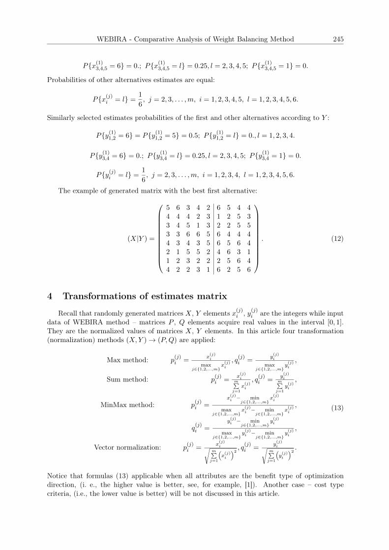
Therefore, the second and all other alternatives are treated as a kind of noise making heavyrecognition of the first – the best alternative. The more alternatives we have, the more difficultis the task of identification.The experiments were carried out with the following parameter values:bXi = 6, i = 1, 2, 3, 4, 5, bYi = 6, i = 1, 2, 3, 4. Probabilities of the first alternative estimates:

P{x(1)1,2 = 6} = P{x(1)

1,2 = 5} = 0.5; P{x(1)1,2 = l} = 0., l = 1, 2, 3, 4.


P{x(1)3,4,5 = 6} = 0.; P{x(1)

3,4,5 = l} = 0.25, l = 2, 3, 4, 5; P{x(1)3,4,5 = 1} = 0.

Probabilities of other alternatives estimates are equal:

P{x(j)i = l} =

1

6, j = 2, 3, . . . ,m, i = 1, 2, 3, 4, 5, l = 1, 2, 3, 4, 5, 6.

Similarly selected estimates probabilities of the first and other alternatives according to Y :

P{y(1)1,2 = 6} = P{y(1)

1,2 = 5} = 0.5; P{y(1)1,2 = l} = 0., l = 1, 2, 3, 4.

P{y(1)3,4 = 6} = 0.; P{y(1)

3,4 = l} = 0.25, l = 2, 3, 4, 5; P{y(1)3,4 = 1} = 0.

P{y(j)i = l} =

1

6, j = 2, 3, . . . ,m, i = 1, 2, 3, 4, l = 1, 2, 3, 4, 5, 6.

The example of generated matrix with the best first alternative:

(X|Y ) =

5 6 3 4 2 6 5 4 44 4 4 2 3 1 2 5 33 4 5 1 3 2 2 5 53 3 6 6 5 6 4 4 44 3 4 3 5 6 5 6 42 1 5 5 2 4 6 3 11 2 3 2 2 2 5 6 44 2 2 3 1 6 2 5 6

. (12)

4 Transformations of estimates matrix

Recall that randomly generated matrices X, Y elements x(j)i , y(j)

i are the integers while inputdata of WEBIRA method – matrices P , Q elements acquire real values in the interval [0, 1].They are the normalized values of matrices X, Y elements. In this article four transformation(normalization) methods (X,Y )→ (P,Q) are applied:

Max method: p(j)i =

x(j)i

maxj∈{1,2,...,m}

x(j)i

, q(j)i =

y(j)i

maxj∈{1,2,...,m}

y(j)i

,

Sum method: p(j)i =

x(j)i

m∑j=1

x(j)i

, q(j)i =

y(j)i

m∑j=1

y(j)i

,

MinMax method: p(j)i =

x(j)i − min

j∈{1,2,...,m}x(j)i

maxj∈{1,2,...,m}

x(j)i − min

j∈{1,2,...,m}x(j)i

,

q(j)i =

y(j)i − min

j∈{1,2,...,m}y(j)i

maxj∈{1,2,...,m}

y(j)i − min

j∈{1,2,...,m}y(j)i

,

Vector normalization: p(j)i =

x(j)i√

m∑j=1

(x(j)i

)2 , q(j)i =

y(j)i√

m∑j=1

(y(j)i

)2 .

(13)

Notice that formulas (13) applicable when all attributes are the benefit type of optimizationdirection, (i. e., the higher value is better, see, for example, [1]). Another case – cost typecriteria, (i.e., the lower value is better) will be not discussed in this article.


Suppose that matrices P , Q and their concatenation – matrix

R = (P |Q) =(r

(j)i

)m×(nx+ny)

, i. e. r(j)i =

{p

(j)i , if i 6 nx,

q(j)i−nx , if nx + 1 6 i 6 nx + ny

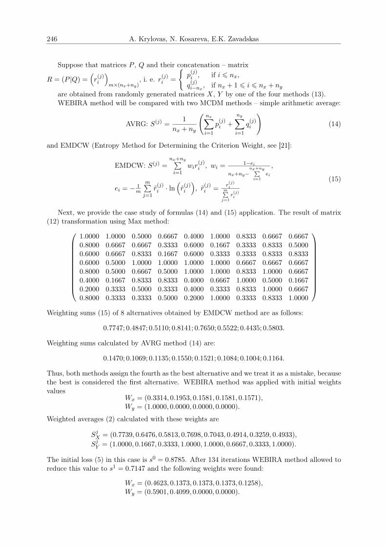
are obtained from randomly generated matrices X, Y by one of the four methods (13).WEBIRA method will be compared with two MCDM methods – simple arithmetic average:

AVRG: S(j) =1

nx + ny

(nx∑i=1

p(j)i +

ny∑i=1

q(j)i

)(14)

and EMDCW (Entropy Method for Determining the Criterion Weight, see [21]:

EMDCW: S(j) =nx+ny∑i=1

wir(j)i , wi = 1−ei

nx+ny−nx+ny∑i=1

ei

,

ei = − 1m

m∑j=1

r(j)i · ln

(r

(j)i

), r

(j)i =

r(j)i

m∑j=1

r(j)i

(15)

Next, we provide the case study of formulas (14) and (15) application. The result of matrix(12) transformation using Max method:

1.0000 1.0000 0.5000 0.6667 0.4000 1.0000 0.8333 0.6667 0.66670.8000 0.6667 0.6667 0.3333 0.6000 0.1667 0.3333 0.8333 0.50000.6000 0.6667 0.8333 0.1667 0.6000 0.3333 0.3333 0.8333 0.83330.6000 0.5000 1.0000 1.0000 1.0000 1.0000 0.6667 0.6667 0.66670.8000 0.5000 0.6667 0.5000 1.0000 1.0000 0.8333 1.0000 0.66670.4000 0.1667 0.8333 0.8333 0.4000 0.6667 1.0000 0.5000 0.16670.2000 0.3333 0.5000 0.3333 0.4000 0.3333 0.8333 1.0000 0.66670.8000 0.3333 0.3333 0.5000 0.2000 1.0000 0.3333 0.8333 1.0000

Weighting sums (15) of 8 alternatives obtained by EMDCW method are as follows:

0.7747; 0.4847; 0.5110; 0.8141; 0.7650; 0.5522; 0.4435; 0.5803.

Weighting sums calculated by AVRG method (14) are:

0.1470; 0.1069; 0.1135; 0.1550; 0.1521; 0.1084; 0.1004; 0.1164.

Thus, both methods assign the fourth as the best alternative and we treat it as a mistake, becausethe best is considered the first alternative. WEBIRA method was applied with initial weightsvalues

Wx = (0.3314, 0.1953, 0.1581, 0.1581, 0.1571),Wy = (1.0000, 0.0000, 0.0000, 0.0000).

Weighted averages (2) calculated with these weights are

SjX = (0.7739, 0.6476, 0.5813, 0.7698, 0.7043, 0.4914, 0.3259, 0.4933),

SjY = (1.0000, 0.1667, 0.3333, 1.0000, 1.0000, 0.6667, 0.3333, 1.0000).

The initial loss (5) in this case is s0 = 0.8785. After 134 iterations WEBIRA method allowed toreduce this value to s1 = 0.7147 and the following weights were found:

Wx = (0.4623, 0.1373, 0.1373, 0.1373, 0.1258),Wy = (0.5901, 0.4099, 0.0000, 0.0000).


Weighted averages are:

SjX = (0.8100, 0.6741, 0.5816, 0.7464, 0.7245, 0.4869, 0.3029, 0.5551),

SjY = (0.9316, 0.2349, 0.3333, 0.8633, 0.9316, 0.8032, 0.5382, 0.7267).

Ranks of alternatives according to the X: 1, 4, 5, 2, 3, 8, 6, 7 and according to the Y : 1, 5, 4,6, 8, 7, 3, 2. So, WEBIRA method set as the best the first alternative and we treat this as theright decision. Notice that all three methods set the same three best alternatives: 1, 4 and 5.

Submit normalized matrices, calculated by other methods. MinMax method:

1.0000 1.0000 0.2500 0.6000 0.2500 1.0000 0.7500 0.3333 0.60000.7500 0.6000 0.5000 0.2000 0.5000 0.0000 0.0000 0.6667 0.40000.5000 0.6000 0.7500 0.0000 0.5000 0.2000 0.0000 0.6667 0.80000.5000 0.4000 1.0000 1.0000 1.0000 1.0000 0.5000 0.3333 0.60000.7500 0.4000 0.5000 0.4000 1.0000 1.0000 0.7500 1.0000 0.60000.2500 0.0000 0.7500 0.8000 0.2500 0.6000 1.0000 0.0000 0.00000.0000 0.2000 0.2500 0.2000 0.2500 0.2000 0.7500 1.0000 0.60000.7500 0.2000 0.0000 0.4000 0.0000 1.0000 0.0000 0.6667 1.0000

.

EMDCW and AVRG methods determined as the best the fifth alternative, WEBIRA – the firstalternative.

Matrix transformated by Sum method:

0.1923 0.2400 0.0937 0.1538 0.0869 0.1818 0.1612 0.1052 0.12900.1538 0.1600 0.1250 0.0769 0.1304 0.0303 0.0645 0.1315 0.09670.1154 0.1600 0.1562 0.0384 0.1304 0.0606 0.0645 0.1315 0.16120.1154 0.1200 0.1875 0.2307 0.2173 0.1818 0.1290 0.1052 0.12900.1538 0.1200 0.1250 0.1153 0.2173 0.1818 0.1612 0.1578 0.12900.0769 0.0400 0.1562 0.1923 0.0869 0.1212 0.1935 0.0789 0.03220.0384 0.0800 0.0937 0.0769 0.0869 0.0606 0.1612 0.1578 0.12900.1538 0.0800 0.0625 0.1153 0.0434 0.1818 0.0645 0.1315 0.1935

.

In this case, as in another – vector normalization method the obtained results coincide withthe Max method, i. e. EMDCW and AVRG methods set as the best the fourth alternative, whileWEBIRA – the first.

Matrix transformated by Vector normalization:

0.5103 0.6155 0.2535 0.3922 0.2222 0.4615 0.4240 0.2917 0.34420.4082 0.4103 0.3380 0.1961 0.3333 0.0769 0.1696 0.3646 0.25810.3061 0.4103 0.4225 0.0980 0.3333 0.1538 0.1696 0.3646 0.43030.3061 0.3077 0.5070 0.5883 0.5556 0.4615 0.3392 0.2917 0.34420.4082 0.3077 0.3380 0.2941 0.5556 0.4615 0.4240 0.4375 0.34420.2041 0.1025 0.4225 0.4902 0.2222 0.3076 0.5089 0.2187 0.08600.1020 0.2051 0.2535 0.1961 0.2222 0.1538 0.4240 0.4375 0.34420.4082 0.2051 0.1690 0.2941 0.1111 0.4615 0.1696 0.3646 0.5163

.

5 Numerical experiments

Numerical experiments were conducted as follows. Random matrices X, Y generated in sucha way that on average more often the best alternative is the first. Matrices P , Q are calculated by


four normalization methods and the best alternative is determined by three methods EMDCW,AVRG andWEBIRA. When the best is the first alternative the result of the experiment is markedwith (+) and recorded to the table. If the best is any other (not the first) alternative (−) isrecorded to the table. It is possible that WEBIRA can not set the best alternative. We thenrecord (n). Notice, that in the cases of EMDCW and AVRG methods such experimental resultis impossible. In the Table 1 the results of 5 experiments are presented. Methods EMDCW,AVRG, WEBIRA are denoted respectively as (E), (A), (W).

Table 1: Fragment of experimental results.

Max method MinMax method Sum method Vector normalizationNr. (E) (A) (W) (E) (A) (W) (E) (A) (W) (E) (A) (W)1 + + + - + + + + + + + +2 + + + + + + + + n + + n3 - - + + - + - - + - - +4 - + + - + + - + + - + +5 - - n - - n - - n - - n

After a series of experiments, we calculate the number of pluses (+) denoted as p in each ofthe 12 columns of the Table 1, the number of minuses (-) denoted as m and undetected cases(n). WEBIRA method peculiarity compared to AVRG and EMDCW – possible non zero valuesof parameter n. It means that WEBIRA quite often eliminates cases when it can not detect thebest alternative. Consider the following indicator to compare methods performance:

En =p−m

p+m+ n. (16)

Indicator En shows reliability of the correspondent method. Our purpose is the detection ofsignificantly different average values of En in the groups.

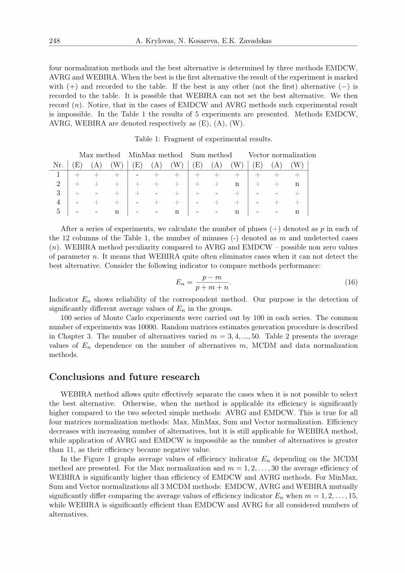
100 series of Monte Carlo experiments were carried out by 100 in each series. The commonnumber of experiments was 10000. Random matrices estimates generation procedure is describedin Chapter 3. The number of alternatives varied m = 3, 4, ..., 50. Table 2 presents the averagevalues of En dependence on the number of alternatives m, MCDM and data normalizationmethods.

Conclusions and future research

WEBIRA method allows quite effectively separate the cases when it is not possible to selectthe best alternative. Otherwise, when the method is applicable its efficiency is significantlyhigher compared to the two selected simple methods: AVRG and EMDCW. This is true for allfour matrices normalization methods: Max, MinMax, Sum and Vector normalization. Efficiencydecreases with increasing number of alternatives, but it is still applicable for WEBIRA method,while application of AVRG and EMDCW is impossible as the number of alternatives is greaterthan 11, as their efficiency became negative value.

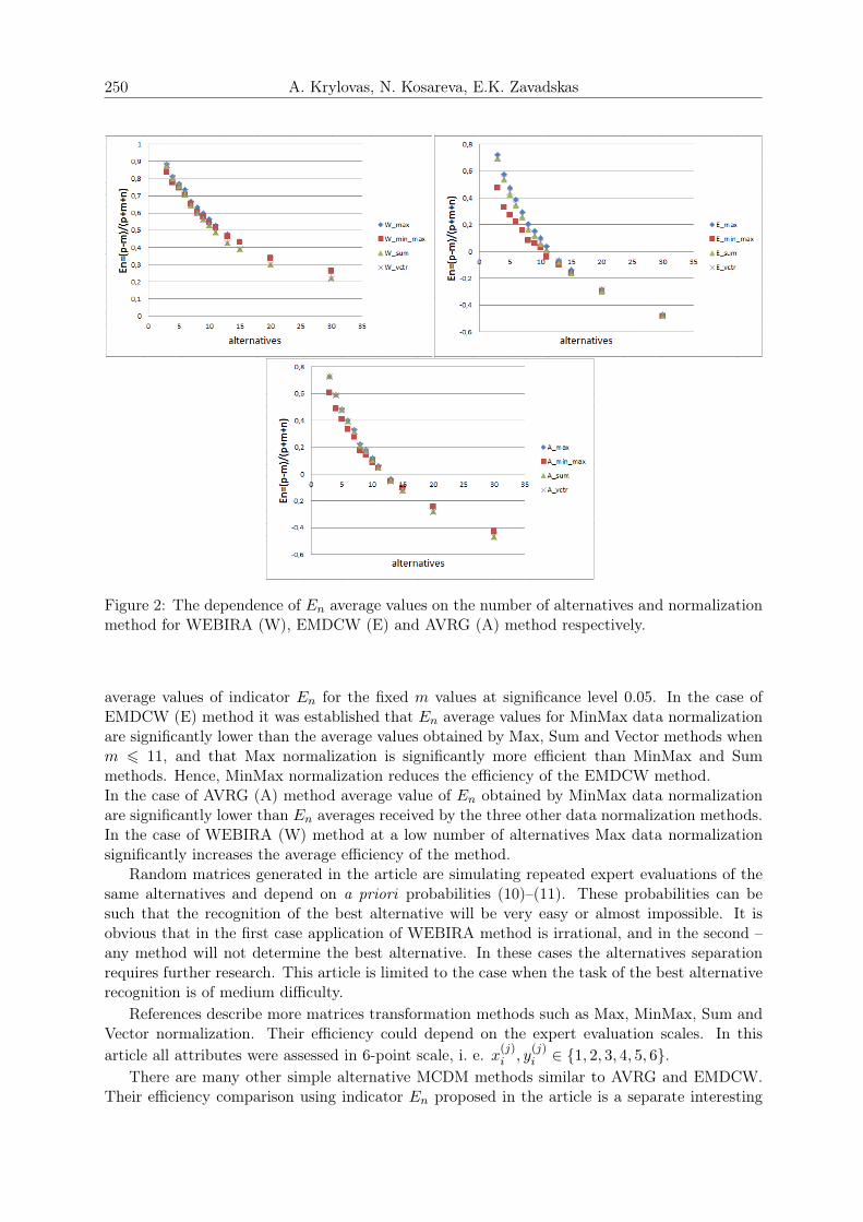
In the Figure 1 graphs average values of efficiency indicator En depending on the MCDMmethod are presented. For the Max normalization and m = 1, 2, . . . , 30 the average efficiency ofWEBIRA is significantly higher than efficiency of EMDCW and AVRG methods. For MinMax,Sum and Vector normalizations all 3 MCDM methods: EMDCW, AVRG and WEBIRA mutuallysignificantly differ comparing the average values of efficiency indicator En when m = 1, 2, . . . , 15,while WEBIRA is significantly efficient than EMDCW and AVRG for all considered numbers ofalternatives.


Table 2: Average values of En dependence on the number of alternatives m, MCDM and datanormalization methods.

Max method MinMax method Sum method Vctr methodm (E) (A) (W) (E) (A) (W) (E) (A) (W) (E) (A) (W)3 0.7224 0.7268 0.8837 0.4736 0.6086 0.8398 0.6944 0.7344 0.8820 0.7018 0.7286 0.88204 0.5762 0.5896 0.8122 0.3298 0.4868 0.7781 0.5358 0.5934 0.8006 0.5468 0.5890 0.80395 0.4760 0.4860 0.7721 0.2746 0.4082 0.7479 0.4288 0.4842 0.7591 0.4438 0.4770 0.75996 0.3870 0.4010 0.7354 0.2220 0.3358 0.7059 0.3426 0.3958 0.7075 0.3552 0.3918 0.70557 0.2968 0.3308 0.6694 0.1580 0.2758 0.6539 0.2556 0.3180 0.6449 0.2682 0.3200 0.64728 0.2060 0.2236 0.6318 0.0824 0.1744 0.6074 0.1606 0.2166 0.6003 0.1782 0.2110 0.60169 0.1520 0.1816 0.5999 0.0626 0.1470 0.5797 0.1134 0.1732 0.5637 0.1272 0.1724 0.5662

10 0.0998 0.1200 0.5644 0.0300 0.0884 0.5430 0.0574 0.1064 0.5314 0.0718 0.1082 0.530011 0.0404 0.0628 0.5275 -0.0412 0.0414 0.5149 0.0108 0.0494 0.4906 0.0168 0.0500 0.490513 -0.0646 -0.0374 0.4745 -0.0992 -0.0556 0.4653 -0.0776 -0.0490 0.4282 -0.0724 -0.0556 0.427415 -0.1356 -0.1032 0.4349 -0.1602 -0.1016 0.4293 -0.1572 -0.1208 0.3943 -0.1534 -0.1220 0.390320 -0.2824 -0.2512 0.3427 -0.2988 -0.2424 0.3378 -0.2930 -0.2786 0.2990 -0.2864 -0.2826 0.298930 -0.4726 -0.4368 0.2639 -0.4840 -0.4272 0.2606 -0.4818 -0.4660 0.2233 -0.4764 -0.4678 0.218350 -0.6592 -0.6250 0.1658 -0.6572 -0.6172 0.1725 -0.6604 -0.6530 0.1482 -0.6616 -0.6524 0.1488

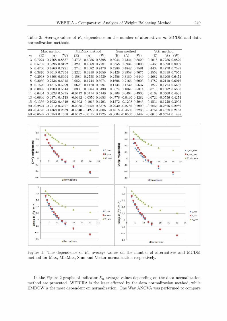
Figure 1: The dependence of En average values on the number of alternatives and MCDMmethod for Max, MinMax, Sum and Vector normalization respectively.

In the Figure 2 graphs of indicator En average values depending on the data normalizationmethod are presented. WEBIRA is the least affected by the data normalization method, whileEMDCW is the most dependent on normalization. One Way ANOVA was performed to compare


Figure 2: The dependence of En average values on the number of alternatives and normalizationmethod for WEBIRA (W), EMDCW (E) and AVRG (A) method respectively.

average values of indicator En for the fixed m values at significance level 0.05. In the case ofEMDCW (E) method it was established that En average values for MinMax data normalizationare significantly lower than the average values obtained by Max, Sum and Vector methods whenm 6 11, and that Max normalization is significantly more efficient than MinMax and Summethods. Hence, MinMax normalization reduces the efficiency of the EMDCW method.In the case of AVRG (A) method average value of En obtained by MinMax data normalizationare significantly lower than En averages received by the three other data normalization methods.In the case of WEBIRA (W) method at a low number of alternatives Max data normalizationsignificantly increases the average efficiency of the method.

Random matrices generated in the article are simulating repeated expert evaluations of thesame alternatives and depend on a priori probabilities (10)–(11). These probabilities can besuch that the recognition of the best alternative will be very easy or almost impossible. It isobvious that in the first case application of WEBIRA method is irrational, and in the second –any method will not determine the best alternative. In these cases the alternatives separationrequires further research. This article is limited to the case when the task of the best alternativerecognition is of medium difficulty.

References describe more matrices transformation methods such as Max, MinMax, Sum andVector normalization. Their efficiency could depend on the expert evaluation scales. In thisarticle all attributes were assessed in 6-point scale, i. e. x(j)

i , y(j)i ∈ {1, 2, 3, 4, 5, 6}.

There are many other simple alternative MCDM methods similar to AVRG and EMDCW.Their efficiency comparison using indicator En proposed in the article is a separate interesting


task. It is appropriate to look for the most efficient methods and investigate the cases when itmakes sense to apply the method WEBIRA.

WEBIRA method is extended and applicable in the case of three or more subgroups ofevaluating criteria. The first direction of our next research is to elaborate WEBIRA metodologyfor solution of practical problems where several groups of criteria naturally arise. For example,for solving sustainable management tasks where several interconnected domains such as ecology,economics, politics and environment are considered. Our other research area is the comparisonof the proposed WEBIRA method with other existing methods used for solving this type ofproblems, i.e. when there are several natural groups of evaluation criteria. The third task is toprepare software for practical MADM problems solving by applying WEBIRA approach.

Bibliography

[1] Stanujkic,D.; Dordevic, B.; Dordevic, M. (2013); Comparative analysis of some prominentMCDM methods: A case of ranking Serbian banks, Serbian Journal of Management, 8(2):213–241.

[2] Zavadskas, E.K.; Turskis, Z. (2008); A New Logarithmic Normalization Method in GamesTheory, Informatica, 19(2): 303–314.

[3] Churchman, C.W.; Ackoff, R. (1954); An Approximate Measure of Value. Journal of theOperations Research Society of America, 2(2):172–187.

[4] Fishburn, P.C. (1967); Additive Utilities with Incomplete Product Sets: Application to Pri-orities and Assignments, Operations Research, 15(3):537–542.

[5] Zionts, S.; Wallenius, J. (1976); An Interactive Programming Method for Solving the MultipleCriteria Problem, Management Science, 26:652–663.

[6] Triantaphyllou, E. (2000); Multi-Criteria Decision Making Methods: A Comparative Study,Norwell, MA:Kluwer.

[7] Stanujkic, D.; Zavadskas, E.K. (2015); A modified Weighted Sum method based on thedecision-maker’s preferred levels of performances, Studies in Informatics and Control, 24(4):461–470.

[8] Alanazi, H.O.; Abdullah, A.H.; Larbani, M. (2013); Dynamic weighted sum multi-criteriadecision making: mathematical model. International Journal of Mathematics and StatisticsInvention, 1(2): 16–18.

[9] Hwang, C.L.; Yoon, K. (1981); Multiple Attribute Decision Making – Methods and Applica-tions: A State-of-the-Art Survey, Lecture Notes in Economics and Mathematical Systems,Springer, New York.

[10] Triantaphyllou, E.; Baig, K. (2005); The impact of aggregating benefit and cost criteria infour MCDA methods, IEEE Transactions on Engineering Management, 52(2):213–226.

[11] Kaliszewski, I.; Podkopaev, D. (2016); Simple additive weighting - A metamodel for multiplecriteria decision analysis methods, Expert Systems with Applications, 54:155–161.

[12] Wang, Y.J. (2015); A fuzzy multi-criteria decision-making model based on simple additiveweighting method and relative preference relation, Applied Soft Computing, 30:412–420.


[13] Tzeng, G.H.; Huang J. (2011); Multiple Attribute Decision Making: Methods and Applica-tions, CRCPress, Taylor & Francis group.

[14] Mardani, A.; Jusoh, A.; Nor, MD K.; Khalifah, Z.; Zakwan, N.; Valipour, A. (2015); Multiplecriteria decision-making techniques and their applications - a review of the literature from2000 to 2014, Economic Research–Ekonomska Istraživanja, 28(1):516–571.

[15] MacCrimmon, K.R. (1968); Decisionmaking Among Multiple-Attribute Alternatives: A Sur-vey and Consolidated Approach, Santa Monica, CA: RAND Corporation.

[16] Wang, P.; Zhu Z.Q.; Wang, Y.G. (2016); A novel hybrid MCDM model combining the SAW,TOPSIS and GRA methods based on experimental design, Information Sciences, 345:27–45.

[17] Ghorabaee, M.K.; Zavadskas, E.K.; Turskis, Z.; Antucheviciene, J. (2016); A new combi-native distance-based assessment (CODAS) method for multi-criteria decision-making, Eco-nomic Computation & Economic Cybernetics Studies & Research, 50(3):25–44.

[18] Chakraborty, S.; Zavadskas, E.K. (2014); Applications of WASPAS Method in Manufactur-ing Decision Making, Informatica, 25(1):1–20.

[19] Zavadskas, E.K.; Antucheviciene, J.; Razavi Hajiagha, S.H; Hashemi, S.S. (2014); Exten-sion of weighted aggregated sum product assessment with interval-valued intuitionistic fuzzynumbers (WASPAS-IVIF), Applied Soft Computing, 24:1013–1021.

[20] Peng, Y.; Zhang, Y.; Kou, G.; Shi, Y. (2012); A Multicriteria Decision Making Approachfor Estimating the Number of Clusters in a Data Set, PLoS ONE, 7(7): e41713.

[21] Zavadskas, E.K.; Podvezko, V. (2016); Integrated Determination of Objective CriteriaWeights in MCDM, International Journal of Information Technology & Decision Making,15(2):267–283.

[22] Krylovas, A.; Zavadskas, E.K.; Kosareva, N.; Dadelo, S. (2014); New KEMIRA Method forDetermining Criteria Priority and Weights in Solving MCDM Problem, International Journalof Information Technology & Decision Making, 13(1):1119–1133.

[23] Krylovas, A.; Kosareva, N.; Zavadskas, E.K. (2016); Statistical analysis of KEMIRA typeweights balancing methods, Romanian Journal of Economic Forecasting, 19(3):19–39.

[24] Krylovas, A.; Zavadskas, E.K.; Kosareva, N. (2016); Multiple criteria decision-makingKEMIRA-M method for solution of location alternatives, Economic Research-EkonomskaIstraživanja, 29(1): 50–65.

[25] Kosareva, N.; Zavadskas, E.K.; Krylovas, A.; Dadelo, S. (2016); Personnel ranking and se-lection problem solution by application of KEMIRA method, International Journal of Com-puters Communications & Control, 11(1):51–66.

[26] Zanakis, S.H.; Solomon, A.; Wishart, N.; Dublish, S. (1998); Multi-attribute decision mak-ing: A simulation comparison of select methods, European Journal of Operational Research,107(3):507–529.

[27] Podvezko, V. (2011); The Comparative Analysis of MCDA Methods SAW and COPRAS,Inzinerine Ekonomika-Engineering Economics, 22(2):134–146.

[28] Mulliner, E.; Malys, N.; Maliene, V. (2016); Comparative analysis of MCDM methods forthe assessment of sustainable housing affordability, Omega, 59(B):146–156.


[29] Karami, A.; Johansson, R. (2014); Utilization of Multi Attribute Decision Making Tech-niques to Integrate Automatic and Manual Ranking of Options, Journal of Information Sci-ence and Engineering, 30(2):519–534.

[30] Kolios, A.; Mytilinou, V.; Lozano-Minguez, E.; Salonitis, K. (2016); A Comparative Study ofMultiple-Criteria Decision-Making Methods under Stochastic Inputs, Energies, 9(7):566–587.

[31] Shannon, C.E. (1948); A Mathematical Theory of Communication, The Bell System Tech-nical J, 27:379–423.

[32] Čereska, A.; Podvezko, V.; Zavadskas, E.K. (2016); Operating Characteristics Analysis ofRotor Systems Using MCDM Methods, Studies in Informatics and Control, 25(1):59–68.

[33] Jahan, A.; Edwards, K.L. (2015); A state-of-the-art survey on the influence of normaliza-tion techniques in ranking: Improving the materials selection process in engineering design,Materials & Design, 65:335–342.

[34] Kaplinski, O.; Tamošaitiene, J. (2015); Analysis of Normalization Methods Influencing Re-sults: A Review to Honour Professor Friedel Peldschus on the Occasion of his 75th Birthday,Procedia Engineering, 122:2–10.

WEBIRA-ComparativeAnalysisofWeightBalancingMethoddspace.vgtu.lt/bitstream/1/3730/1/WEBIRA -...

Documents

Transcript of WEBIRA-ComparativeAnalysisofWeightBalancingMethoddspace.vgtu.lt/bitstream/1/3730/1/WEBIRA -...