web.eecs.umich.eduweb.eecs.umich.edu/~hero/Preprints/10.1007_s10618-012-0302-x.pdf · Adaptive...

1 23

Data Mining and KnowledgeDiscovery ISSN 1384-5810 Data Min Knowl DiscDOI 10.1007/s10618-012-0302-x

Adaptive evolutionary clustering

Kevin S. Xu, Mark Kliger & AlfredO. Hero III

1 23

Your article is protected by copyright and all

rights are held exclusively by The Author(s).

This e-offprint is for personal use only

and shall not be self-archived in electronic

repositories. If you wish to self-archive your

work, please use the accepted author’s

version for posting to your own website or

your institution’s repository. You may further

deposit the accepted author’s version on

a funder’s repository at a funder’s request,

provided it is not made publicly available until

12 months after publication.

Data Min Knowl DiscDOI 10.1007/s10618-012-0302-x


Kevin S. Xu · Mark Kliger · Alfred O. Hero III

Received: 10 April 2011 / Accepted: 21 December 2012© The Author(s) 2013

Abstract In many practical applications of clustering, the objects to be clusteredevolve over time, and a clustering result is desired at each time step. In such applica-tions, evolutionary clustering typically outperforms traditional static clustering by pro-ducing clustering results that reflect long-term trends while being robust to short-termvariations. Several evolutionary clustering algorithms have recently been proposed,often by adding a temporal smoothness penalty to the cost function of a static cluster-ing method. In this paper, we introduce a different approach to evolutionary clusteringby accurately tracking the time-varying proximities between objects followed by staticclustering. We present an evolutionary clustering framework that adaptively estimatesthe optimal smoothing parameter using shrinkage estimation, a statistical approachthat improves a naïve estimate using additional information. The proposed frameworkcan be used to extend a variety of static clustering algorithms, including hierarchical,k-means, and spectral clustering, into evolutionary clustering algorithms. Experimentson synthetic and real data sets indicate that the proposed framework outperforms staticclustering and existing evolutionary clustering algorithms in many scenarios.

Responsible editor: Ian Davidson.

K. S. Xu (B)· A. O. Hero IIIEECS Department, University of Michigan, 1301 Beal Avenue, Ann Arbor, MI 48109-2122, USAe-mail: [email protected]

A. O. Hero IIIe-mail: [email protected]

M. KligerOmek Interactive, Bet Shemesh, Israele-mail: [email protected]

123

Author's personal copy

K. S. Xu et al.

Keywords Evolutionary clustering · Similarity measures · Clustering algorithms ·Tracking · Data smoothing · Adaptive filtering · Shrinkage estimation

1 Introduction

In many practical applications of clustering, the objects to be clustered are observedat many points in time, and the goal is to obtain a clustering result at each time step.This situation arises in applications such as identifying communities in dynamic socialnetworks (Falkowski et al. 2006; Tantipathananandh et al. 2007), tracking groups ofmoving objects (Li et al. 2004; Carmi et al. 2009), finding time-varying clusters ofstocks or currencies in financial markets (Fenn et al. 2009), and many other applicationsin data mining, machine learning, and signal processing. Typically the objects evolveover time both as a result of long-term drifts due to changes in their statistical propertiesand short-term variations due to noise.

A naïve approach to these types of problems is to perform static clustering at eachtime step using only the most recent data. This approach is extremely sensitive to noiseand produces clustering results that are unstable and inconsistent with clustering resultsfrom adjacent time steps. Subsequently, evolutionary clustering methods have beendeveloped, with the goal of producing clustering results that reflect long-term driftsin the objects while being robust to short-term variations.1

Several evolutionary clustering algorithms have recently been proposed by addinga temporal smoothness penalty to the cost function of a static clustering method. Thispenalty prevents the clustering result at any given time from deviating too much fromthe clustering results at neighboring time steps. This approach has produced evolu-tionary extensions of commonly used static clustering methods such as agglomerativehierarchical clustering (Chakrabarti et al. 2006), k-means (Chakrabarti et al. 2006),Gaussian mixture models (Zhang et al. 2009), and spectral clustering (Tang et al. 2008;Chi et al. 2009) among others. How to choose the weight of the penalty in an optimalmanner in practice, however, remains an open problem.

In this paper, we propose a different approach to evolutionary clustering by treatingit as a problem of tracking followed by static clustering (Sect. 3). We model theobserved matrix of proximities between objects at each time step, which can be eithersimilarities or dissimilarities, as a linear combination of a true proximity matrix and azero-mean noise matrix. The true proximities, which vary over time, can be viewed asunobserved states of a dynamic system. Our approach involves estimating these statesusing both current and past proximities, then performing static clustering on the stateestimates.

The states are estimated using a restricted class of estimators known as shrinkageestimators, which improve a raw estimate by combining it with other information. Wedevelop a method for estimating the optimal weight to place on past proximities soas to minimize the mean squared error (MSE) between the true proximities and ourestimates. We call this weight the forgetting factor. One advantage of our approach

1 The term “evolutionary clustering” has also been used to refer to clustering algorithms motivated bybiological evolution, which are unrelated to the methods discussed in this paper.

123



is that it provides an explicit formula for the optimal forgetting factor, unlike existingevolutionary clustering methods. The forgetting factor is estimated adaptively, whichallows it to vary over time to adjust to the conditions of the dynamic system.

The proposed framework, which we call Adaptive Forgetting Factor for Evolution-ary Clustering and Tracking (AFFECT), can extend any static clustering algorithm thatuses pairwise similarities or dissimilarities into an evolutionary clustering algorithm. Itis flexible enough to handle changes in the number of clusters over time and to accom-modate objects entering and leaving the data set between time steps. We demonstratehow AFFECT can be used to extend three popular static clustering algorithms, namelyhierarchical clustering, k-means, and spectral clustering, into evolutionary clusteringalgorithms (Sect. 4). These algorithms are tested on several synthetic and real datasets (Sect. 5). We find that they not only outperform static clustering, but also otherrecently proposed evolutionary clustering algorithms due to the adaptively selectedforgetting factor.

The main contribution of this paper is the development of the AFFECT adaptiveevolutionary clustering framework, which has several advantages over existing evo-lutionary clustering approaches:

1. It involves smoothing proximities between objects over time followed by staticclustering, which enables it to extend any static clustering algorithm that takes aproximity matrix as input to an evolutionary clustering algorithm.

2. It provides an explicit formula and estimation procedure for the optimal weight(forgetting factor) to apply to past proximities.

3. It outperforms static clustering and existing evolutionary clustering algorithms inseveral experiments with a minimal increase in computation time compared tostatic clustering (if a single iteration is used to estimate the forgetting factor).

This paper is an extension of our previous work (Xu et al. 2010), which was limitedto evolutionary spectral clustering. In this paper, we extend the previously proposedframework to other static clustering algorithms. We also provide additional insightinto the model assumptions in Xu et al. (2010) and demonstrate the effectiveness ofAFFECT in several additional experiments.

2 Background

2.1 Static clustering algorithms

We begin by reviewing three commonly used static clustering algorithms. We demon-strate the evolutionary extension of these algorithms in Sect. 4, although the AFFECTframework can be used to extend many other static clustering algorithms. The term“clustering” is used in this paper to refer to both data clustering and graph clustering.The notation i ∈ c is used to denote object i being assigned to cluster c. |c| denotesthe number of objects in cluster c, and C denotes a clustering result (the set of allclusters).

In the case of data clustering, we assume that the n objects in the data set are storedin an n × p matrix X , where object i is represented by a p-dimensional feature vectorxi corresponding to the i th row of X . From these feature vectors, one can create a

123


K. S. Xu et al.

Fig. 1 A general agglomerativehierarchical clustering algorithm

1: Assign each object to its own cluster2: repeat3: Compute dissimilarities between each pair of clusters4: Merge clusters with the lowest dissimilarity5: until all objects are merged into one cluster6: return dendrogram

proximity matrix W , wherewi j denotes the proximity between objects i and j , whichcould be their Euclidean distance or any other similarity or dissimilarity measure.

For graph clustering, we assume that the n vertices in the graph are representedby an n × n adjacency matrix W where wi j denotes the weight of the edge betweenvertices i and j . If there is no edge between i and j , then wi j = 0. For the usualcase of undirected graphs with non-negative edge weights, an adjacency matrix is asimilarity matrix, so we shall refer to it also as a proximity matrix.

2.1.1 Agglomerative hierarchical clustering

Agglomerative hierarchical clustering algorithms are greedy algorithms that createa hierarchical clustering result, often represented by a dendrogram (Hastie et al. 2001).The dendrogram can be cut at a certain level to obtain a flat clustering result. Thereare many variants of agglomerative hierarchical clustering. A general algorithm isdescribed in Fig. 1. Varying the definition of dissimilarity between a pair of clustersoften changes the clustering results. Three common choices are to use the minimumdissimilarity between objects in the two clusters (single linkage), the maximum dis-similarity (complete linkage), or the average dissimilarity (average linkage) (Hastieet al. 2001).

2.1.2 k-means

k-means clustering (MacQueen 1967; Hastie et al. 2001) attempts to find clusters thatminimize the sum of squares cost function

D(X,C ) =k∑

c=1

∑

i∈c

‖xi − mc‖2, (1)

where ‖ · ‖ denotes the �2-norm, and mc is the centroid of cluster c, given by

mc =∑

i∈c xi

|c| .

Each object is assigned to the cluster with the closest centroid. The cost of a clusteringresult C is simply the sum of squared Euclidean distances between each object andits closest centroid. The squared distance in (1) can be rewritten as

‖xi − mc‖2 = wi i − 2∑

j∈c wi j

|c| +∑

j,l∈c w jl

|c|2 , (2)

123



Fig. 2 Pseudocode for k-means clustering using similarity matrix W

where wi j = xi xTj , the dot product of the feature vectors. Using the form of (2) to

compute the k-means cost in (1) allows the k-means algorithm to be implemented withonly the similarity matrix W = [wi j ]n

i, j=1 consisting of all pairs of dot products, asdescribed in Fig. 2.

2.1.3 Spectral clustering

Spectral clustering (Shi and Malik 2000; Ng et al. 2001; von Luxburg 2007) is a pop-ular modern clustering technique inspired by spectral graph theory. It can be used forboth data and graph clustering. When used for data clustering, the first step in spectralclustering is to create a similarity graph with vertices corresponding to the objects andedge weights corresponding to the similarities between objects. We represent the graphby an adjacency matrix W with edge weights wi j given by a positive definite similar-ity function s(xi , x j ). The most commonly used similarity function is the Gaussiansimilarity function s(xi , x j ) = exp{−‖xi − x j‖2/(2ρ2)} (Ng et al. 2001), where ρ isa scaling parameter. Let D denote a diagonal matrix with elements corresponding torow sums of W . Define the unnormalized graph Laplacian matrix by L = D − W andthe normalized Laplacian matrix (Chung 1997) by L = I − D−1/2W D−1/2.

Three common variants of spectral clustering are average association (AA), ratio cut(RC), and normalized cut (NC) (Shi and Malik 2000). Each variant is associated withan NP-hard graph optimization problem. Spectral clustering solves relaxed versionsof these problems. The relaxed problems can be written as (von Luxburg 2007; Chi etal. 2009)

AA(Z) = maxZ∈Rn×k

tr(Z T W Z) subject to Z T Z = I (3)

RC(Z) = minZ∈Rn×k

tr(Z T L Z) subject to Z T Z = I (4)

NC(Z) = minZ∈Rn×k

tr(Z T L Z) subject to Z T Z = I. (5)

These are variants of a trace optimization problem; the solutions are given by a gen-eralized Rayleigh-Ritz theorem (Lütkepohl 1997). The optimal solution to (3) consistsof the matrix containing the eigenvectors corresponding to the k largest eigenvalues ofW as columns. Similarly, the optimal solutions to (4) and (5) consist of the matricescontaining the eigenvectors corresponding to the k smallest eigenvalues of L and L ,respectively. The optimal relaxed solution Z is then discretized to obtain a clustering

123


K. S. Xu et al.

Fig. 3 Pseudocode fornormalized cut spectralclustering

result, typically by running the standard k-means algorithm on the rows of Z or anormalized version of Z .

An algorithm (Ng et al. 2001) for normalized cut spectral clustering is shown inFig. 3. To perform ratio cut spectral clustering, compute eigenvectors of L insteadof L and ignore the row normalization in steps 2–4. Similarly, to perform averageassociation spectral clustering, compute instead the k largest eigenvectors of W andignore the row normalization in steps 2–4.

2.2 Related work

We now summarize some contributions in the related areas of incremental and con-strained clustering, as well as existing work on evolutionary clustering.

2.2.1 Incremental clustering

The term “incremental clustering” has typically been used to describe two types ofclustering problems2:

1. Sequentially clustering objects that are each observed only once.2. Clustering objects that are each observed over multiple time steps.

Type 1 is also known as data stream clustering, and the focus is on clustering the datain a single pass and with limited memory (Charikar et al. 2004; Gupta and Grossman2004). It is not directly related to our work because in data stream clustering eachobject is observed only once.

Type 2 is of greater relevance to our work and targets the same problem setting asevolutionary clustering. Several incremental algorithms of this type have been pro-posed (Li et al. 2004; Sun et al. 2007; Ning et al. 2010). These incremental clusteringalgorithms could also be applied to the type of problems we consider; however, thefocus of incremental clustering is on low computational cost at the expense of clus-tering quality. The incremental clustering result is often worse than the result of per-forming static clustering at each time step, which is already a suboptimal approach asmentioned in the introduction. On the other hand, evolutionary clustering is concernedwith improving clustering quality by intelligently combining data from multiple timesteps and is capable of outperforming static clustering.

2 It is also sometimes used to refer to the simple approach of performing static clustering at each time step.

123



2.2.2 Constrained clustering

The objective of constrained clustering is to find a clustering result that optimizessome goodness-of-fit objective (such as the k-means sum of squares cost function(1)) subject to a set of constraints. The constraints can either be hard or soft. Hardconstraints can be used, for example, to specify that two objects must or must not be inthe same cluster (Wagstaff et al. 2001; Wang and Davidson 2010). On the other hand,soft constraints can be used to specify real-valued preferences, which may be obtainedfrom labels or other prior information (Ji and Xu 2006; Wang and Davidson 2010).These soft constraints are similar to evolutionary clustering in that they bias clusteringresults based on additional information; in the case of evolutionary clustering, theadditional information could correspond to historical data or clustering results.

Tadepalli et al. (2009) considered the problem of clustering time-evolving objectssuch that objects in the same cluster at a particular time step are unlikely to be in thesame cluster at the following time step. Such an approach allows one to divide the timeseries into segments that differ significantly from one another. Notice that this is theopposite of the evolutionary clustering objective, which favors smooth evolutions incluster memberships over time. Hossain et al. (2010) proposed a framework that unifiesthese two objectives, which are referred to as disparate and dependent clustering,respectively. Both can be viewed as clustering with soft constraints to minimize ormaximize similarity between multiple sets of clusters, e.g. clusters at different timesteps.

2.2.3 Evolutionary clustering

The topic of evolutionary clustering has attracted significant attention in recent years.Chakrabarti et al. (2006) introduced the problem and proposed a general frameworkfor evolutionary clustering by adding a temporal smoothness penalty to a static clus-tering method. Evolutionary extensions for agglomerative hierarchical clustering andk-means were presented as examples of the framework.

Chi et al. (2009) expanded on this idea by proposing two frameworks for evolu-tionary spectral clustering, which they called Preserving Cluster Quality (PCQ) andPreserving Cluster Membership (PCM). Both frameworks proposed to optimize themodified cost function

Ctotal = α Ctemporal + (1 − α)Csnapshot, (6)

where Csnapshot denotes the static spectral clustering cost, which is typically taken tobe the average association, ratio cut, or normalized cut as discussed in Sect. 2.1.3. Thetwo frameworks differ in how the temporal smoothness penalty Ctemporal is defined.In PCQ, Ctemporal is defined to be the cost of applying the clustering result at time tto the similarity matrix at time t − 1. In other words, it penalizes clustering resultsthat disagree with past similarities. In PCM, Ctemporal is defined to be a measure ofdistance between the clustering results at time t and t − 1. In other words, it penalizesclustering results that disagree with past clustering results. Both choices of temporalcost are quadratic in the cluster memberships, similar to the static spectral clustering

123


K. S. Xu et al.

cost as in (3)–(5), so optimizing (6) in either case is simply a trace optimizationproblem. For example, the PCQ average association evolutionary spectral clusteringproblem is given by

maxZ∈Rn×k

αtr(

Z T W t−1 Z)

+ (1 − α)tr(

Z T W t Z)

subject to Z T Z = I,

where W t and W t−1 denote the adjacency matrices at times t and t − 1, respec-tively. The PCQ cluster memberships can be found by computing eigenvectors ofαW t−1 + (1 −α)W t and then discretizing as discussed in Sect. 2.1.3. Our work takesa different approach than that of Chi et al. (2009) but the resulting framework sharessome similarities with the PCQ framework. In particular, AFFECT paired with aver-age association spectral clustering is an extension of PCQ to longer history, which wediscuss in Sect. 4.3.

Following these works, other evolutionary clustering algorithms that attempt tooptimize the modified cost function defined in (6) have been proposed (Tang et al.2008; Lin et al. 2009; Zhang et al. 2009; Mucha et al. 2010). The definitions of snap-shot and temporal cost and the clustering algorithms vary by approach. None of theaforementioned works addresses the problem of how to choose the parameter α in(6), which determines how much weight to place on historic data or clustering results.It has typically been suggested (Chi et al. 2009; Lin et al. 2009) to choose it in anad-hoc manner according to the user’s subjective preference on the temporal smooth-ness of the clustering results.

It could also be beneficial to allow α to vary with time. Zhang et al. (2009) proposedto choose α adaptively by using a test statistic for checking dependency between twodata sets (Gretton et al. 2007). However, this test statistic also does not satisfy any opti-mality properties for evolutionary clustering and still depends on a global parameterreflecting the user’s preference on temporal smoothness, which is undesirable.

The existing method that is most similar to AFFECT is that of Rosswog and Ghose(2008), which we refer to as RG. The authors proposed evolutionary extensions ofk-means and agglomerative hierarchical clustering by filtering the feature vectors usinga Finite Impulse Response (FIR) filter, which combines the last l + 1 measurementsof the feature vectors by the weighted sum yt

i = b0xti + b1xt−1

i + · · · + blxt−li , where

l is the order of the filter, yti is the filter output at time t , and b0, . . . , bl are the filter

coefficients. The proximities are then calculated between the filter outputs rather thanthe feature vectors. The main resemblance between RG and AFFECT is that RG is alsobased on tracking followed by static clustering. In particular, RG adaptively selectsthe filter coefficients based on the dissimilarities between cluster centroids at the past ltime steps. However, RG cannot accommodate varying numbers of clusters over timenor can it deal with objects entering and leaving at various time steps. It also strugglesto adapt to changes in clusters, as we demonstrate in Sect. 5.2. AFFECT, on the otherhand, is able to adapt quickly to changes in clusters and is applicable to a much largerclass of problems.

Finally, there has also been recent interest in model-based evolutionary clustering.In addition to the aforementioned method involving mixtures of exponential families(Zhang et al. 2009), methods have also been proposed using semi-Markov models

123



(Wang et al. 2007), Dirichlet process mixtures (DPMs) (Ahmed and Xing 2008; Xu etal. 2008a), hierarchical DPMs (Xu et al. 2008a,b; Zhang et al. 2010), and smooth plaidmodels (Mankad et al. 2011). For these methods, the temporal evolution is controlledby hyperparameters that can be estimated in some cases.

3 Proposed evolutionary framework

The proposed framework treats evolutionary clustering as a tracking problem followedby ordinary static clustering. In the case of data clustering, we assume that the featurevectors have already been converted into a proximity matrix, as discussed in Sect. 2.1.We treat the proximity matrices, denoted by W t , as realizations from a non-stationaryrandom process indexed by discrete time steps, denoted by the superscript t . Weassume, like many other evolutionary clustering algorithms, that the identities of theobjects can be tracked over time so that the rows and columns of W t correspond tothe same objects as those of W t−1 provided that no objects are added or removed(we describe how the proposed framework handles adding and removing objects inSect. 4.4.1). Furthermore we posit the linear observation model

W t = Ψ t + N t , t = 0, 1, 2, . . . (7)

where Ψ t is an unknown deterministic matrix of unobserved states, and N t is a zero-mean noise matrix.Ψ t changes over time to reflect long-term drifts in the proximities.We refer to Ψ t as the true proximity matrix, and our goal is to accurately estimate itat each time step. On the other hand, N t reflects short-term variations due to noise.Thus we assume that N t , N t−1, . . . , N 0 are mutually independent.

A common approach for tracking unobserved states in a dynamic system is to use aKalman filter (Harvey 1989; Haykin 2001) or some variant. Since the states correspondto the true proximities, there are O(n2) states and O(n2) observations, which makesthe Kalman filter impractical for two reasons. First, it involves specifying a parametricmodel for the state evolution over time, and secondly, it requires the inversion of anO(n2)× O(n2) covariance matrix, which is large enough in most evolutionary clus-tering applications to make matrix inversion computationally infeasible. We present asimpler approach that involves a recursive update of the state estimates using only asingle parameter αt , which we define in (8).

3.1 Smoothed proximity matrix

If the true proximity matrix Ψ t is known, we would expect to see improved clusteringresults by performing static clustering on Ψ t rather than on the current proximitymatrix W t because Ψ t is free from noise. Our objective is to accurately estimate Ψ t

at each time step. We can then perform static clustering on our estimate, which shouldalso lead to improved clustering results.

The naïve approach of performing static clustering on W t at each time step can beinterpreted as using W t itself as an estimate for Ψ t . The main disadvantage of thisapproach is that it suffers from high variance due to the observation noise N t . As a

123


K. S. Xu et al.

consequence, the obtained clustering results can be highly unstable and inconsistentwith clustering results from adjacent time steps.

A better estimate can be obtained using the smoothed proximity matrix Ψ t definedby

Ψ t = αt Ψ t−1 + (1 − αt )W t (8)

for t ≥ 1 and by Ψ 0 = W 0. Notice that Ψ t is a function of current and past dataonly, so it can be computed in the on-line setting where a clustering result for time t isdesired before data at time t +1 can be obtained. Ψ t incorporates proximities not onlyfrom time t − 1, but potentially from all previous time steps and allows us to suppressthe observation noise. The parameter αt controls the rate at which past proximitiesare forgotten; hence we refer to it as the forgetting factor. The forgetting factor in ourframework can change over time, allowing the amount of temporal smoothing to vary.

3.2 Shrinkage estimation of true proximity matrix

The smoothed proximity matrix Ψ t is a natural candidate for estimating Ψ t . It is aconvex combination of two estimators: W t and Ψ t−1. Since N t is zero-mean, W t isan unbiased estimator but has high variance because it uses only a single observation.Ψ t−1 is a weighted combination of past observations so it should have lower variancethan W t , but it is likely to be biased since the past proximities may not be represen-tative of the current ones as a result of long-term drift in the statistical properties ofthe objects. Thus the problem of estimating the optimal forgetting factor αt may beconsidered as a bias-variance trade-off problem.

A similar bias-variance trade-off has been investigated in the problem of shrinkageestimation of covariance matrices (Ledoit and Wolf 2003; Schäfer and Strimmer 2005;Chen et al. 2010), where a shrinkage estimate of the covariance matrix is taken to be� = λT +(1−λ)S, a convex combination of a suitably chosen target matrix T and thestandard estimate, the sample covariance matrix S. Notice that the shrinkage estimatehas the same form as the smoothed proximity matrix given by (8) where the smoothedproximity matrix at the previous time step Ψ t−1 corresponds to the shrinkage targetT , the current proximity matrix W t corresponds to the sample covariance matrix S,and αt corresponds to the shrinkage intensity λ. We derive the optimal choice of αt

in a manner similar to Ledoit and Wolf’s derivation of the optimal λ for shrinkageestimation of covariance matrices (Ledoit and Wolf 2003).

As in Ledoit and Wolf (2003), Schäfer and Strimmer (2005), and Chen et al. (2010),we choose to minimize the squared Frobenius norm of the difference between the trueproximity matrix and the smoothed proximity matrix. That is, we take the loss functionto be

L(αt) =

∥∥∥Ψ t − Ψ t∥∥∥

2

F=

n∑

i=1

n∑

j=1

(ψ t

i j − ψ ti j

)2.

123



We define the risk to be the conditional expectation of the loss function given allof the previous observations

R(αt) = E

[∥∥∥Ψ t − Ψ t∥∥∥

2

F

∣∣∣∣ W (t−1)]

where W (t−1) denotes the set{W t−1,W t−2, . . . ,W 0

}. Note that the risk function is

differentiable and can be easily optimized ifΨ t is known. However,Ψ t is the quantitythat we are trying to estimate so it is not known. We first derive the optimal forgettingfactor assuming it is known. We shall henceforth refer to this as the oracle forgettingfactor.

Under the linear observation model of (7),

E[W t

∣∣W (t−1)]

= E[W t ] = Ψ t (9)

var(

W t∣∣W (t−1)

)= var

(W t) = var

(N t) (10)

because N t, N t−1, . . . , N 0 are mutually independent and have zero mean. From thedefinition of Ψ t in (8), the risk can then be expressed as

R(αt) =

n∑

i=1

n∑

j=1

E

[(αt ψ t−1

i j + (1 − αt)wt

i j − ψ ti j

)2∣∣∣∣ W (t−1)

]

=n∑

i=1

n∑

j=1

{var

(αt ψ t−1

i j + (1 − αt)wt

i j − ψ ti j

∣∣∣ W (t−1))

+E[αt ψ t−1

i j + (1 − αt)wt

i j − ψ ti j

∣∣∣ W (t−1)]2

}. (11)

(11) can be simplified using (9) and (10) and by noting that the conditional varianceof ψ t−1

i j is zero and that ψ ti j is deterministic. Thus

R(αt) =

n∑

i=1

n∑

j=1

{(1 − αt)2 var

(nt

i j

)+ (αt)2

(ψ t−1

i j − ψ ti j

)2}. (12)

From (12), the first derivative is easily seen to be

R′(αt) = 2n∑

i=1

n∑

j=1

{(αt − 1

)var

(nt

i j

)+ αt

(ψ t−1

i j − ψ ti j

)2}.

123


K. S. Xu et al.

To determine the oracle forgetting factor(αt

)∗, simply set R′(αt) = 0. Rearranging

to isolate αt , we obtain

(αt)∗ =

n∑i=1

n∑j=1

var(

nti j

)

n∑i=1

n∑j=1

{(ψ t−1

i j − ψ ti j

)2 + var(

nti j

)} . (13)

We find that(αt

)∗ does indeed minimize the risk because R′′(αt) ≥ 0 for all αt .

The oracle forgetting factor(αt

)∗ leads to the best estimate in terms of minimizingrisk but is not implementable because it requires oracle knowledge of the true proximitymatrix Ψ t , which is what we are trying to estimate, as well as the noise variancevar

(N t

). It was suggested in Schäfer and Strimmer (2005) to replace the unknowns

with their sample equivalents. In this setting, we would replace ψ ti j with the sample

mean of wti j and var(nt

i j ) = var(wti j ) with the sample variance of wt

i j . However, Ψ t

and potentially var(N t

)are time-varying so we cannot simply use the temporal sample

mean and variance. Instead, we propose to use the spatial sample mean and variance.Since objects belong to clusters, it is reasonable to assume that the structure of Ψ t

and var(N t

)should reflect the cluster memberships. Hence we make an assumption

about the structure of Ψ t and var(N t

)in order to proceed.

3.3 Block model for true proximity matrix

We propose a block model for the true proximity matrix Ψ t and var(N t

)and use the

assumptions of this model to compute the desired sample means and variances. Theassumptions of the block model are as follows:

1. ψ ti i = ψ t

j j for any two objects i, j that belong to the same cluster.2. ψ t

i j = ψ tlm for any two distinct objects i, j and any two distinct objects l,m such

that i, l belong to the same cluster, and j,m belong to the same cluster.

The structure of the true proximity matrix Ψ t under these assumptions is shown inFig. 4. In short, we are assuming that the true proximity is equal inside the clustersand different between clusters. We make the assumptions on var

(N t

)that we do on

Ψ t , namely that it also possesses the assumed block structure.One scenario where the block assumptions are completely satisfied is the case where

the data at each time t are realizations from a dynamic Gaussian mixture model (GMM)(Carmi et al. 2009), which is described as follows. Assume that the k components ofthe dynamic GMM are parameterized by the k time-varying mean vectors

{µt

c

}kc=1

and covariance matrices{Σ t

c

}kc=1. Let {φc}k

c=1 denote the mixture weights. Objectsare sampled in the following manner:

1. (Only at t = 0) Draw n samples {zi }ni=1 from the categorical distribution specified

by {φc}kc=1 to determine the component membership of each object.

2. (For all t) For each object i , draw a sample xti from the Gaussian distribution

parameterized by(µt

zi, �t

zi

).

123



Fig. 4 Block structure of trueproximity matrix Ψ t . ψ t

(c)denotes ψ t

i i for all objects i incluster c, and ψ t

(cd) denotes ψ ti j

for all distinct objects i, j suchthat i is in cluster c and j is incluster d

Notice that while the parameters of the individual components change over time,the component memberships do not, i.e. objects stay in the same components overtime. The dynamic GMM simulates clusters moving in time. In Appendix A.1, weshow that at each time t , the mean and variance of the dot product similarity matrixW t , which correspond to Ψ t and var

(N t

)respectively under the observation model

of (7), do indeed satisfy the assumed block structure. This scenario forms the basis ofthe experiment in Sect. 5.1.

Although the proposed block model is rather simplistic, we believe that it is areasonable choice when there is no prior information about the shapes of clusters. Asimilar block assumption has also been used in the dynamic stochastic block model(Yang et al. 2011), developed for modeling dynamic social networks. A nice featureof the proposed block model is that it is permutation invariant with respect to theclusters; that is, it does not require objects to be ordered in any particular manner.The extension of the proposed framework to other models is beyond the scope of thispaper and is an area for future work.

3.4 Adaptive estimation of forgetting factor

Under the block model assumption, the means and variances of proximities are iden-tical in each block. As a result, we can sample over all proximities in a block to obtainsample means and variances. Unfortunately, we do not know the true block structurebecause the cluster memberships are unknown.

To work around this problem, we estimate the cluster memberships along with (αt )∗in an iterative fashion. First we initialize the cluster memberships. Two logical choicesare to use the cluster memberships from the previous time step or the membershipsobtained from performing static clustering on the current proximities. We can thensample over each block to estimate the entries of Ψ t and var(N t ) as detailed below,and substitute them into (13) to obtain an estimate (αt )∗ of (αt )∗. Now substitute (αt )∗into (8) and perform static clustering on Ψ t to obtain an updated clustering result. Thisclustering result is then used to refine the estimate of (αt )∗, and this iterative processis repeated to improve the quality of the clustering result. We find, empirically, thatthe estimated forgetting factor rarely changes after the third iteration and that even asingle iteration often provides a good estimate.

123


K. S. Xu et al.

Fig. 5 Pseudocode for generic AFFECT evolutionary clustering algorithm. Cluster(·) denotes any staticclustering algorithm that takes a similarity or dissimilarity matrix as input and returns a flat clustering result

To estimate the entries of Ψ t = E[W t

], we proceed as follows. For two distinct

objects i and j both in cluster c, we estimate ψ ti j using the sample mean

E[wt

i j

]= 1

|c| (|c| − 1)

∑

l∈c

∑

m∈cm �=l

wtlm .

Similarly, we estimate ψ ti i by

E[wt

i i

] = 1

|c|∑

l∈c

wtll .

For distinct objects i in cluster c and j in cluster d with c �= d, we estimate ψ ti j by

E[wt

i j

]= 1

|c||d|∑

l∈c

∑

m∈d

wtlm .

var(N t

) = var(W t

)can be estimated in a similar manner by taking unbiased sample

variances over the blocks.

4 Evolutionary algorithms

From the derivation in Sect. 3.4, we have the generic algorithm for AFFECT at eachtime step shown in Fig. 5. We provide some details and interpretation of this genericalgorithm when used with three popular static clustering algorithms: agglomerativehierarchical clustering, k-means, and spectral clustering.

4.1 Agglomerative hierarchical clustering

The proposed evolutionary extension of agglomerative hierarchical clustering has aninteresting interpretation in terms of the modified cost function defined in (6). Recallthat agglomerative hierarchical clustering is a greedy algorithm that merges the twoclusters with the lowest dissimilarity at each iteration. The dissimilarity between two

123



clusters can be interpreted as the cost of merging them. Thus, performing agglomer-ative hierarchical clustering on Ψ t results in merging the two clusters with the lowestmodified cost at each iteration. The snapshot cost of a merge corresponds to the costof making the merge at time t using the dissimilarities given by W t . The temporal costof a merge is a weighted combination of the costs of making the merge at each timestep s ∈ {0, 1, . . . , t − 1} using the dissimilarities given by W s . This can be seen byexpanding the recursive update in (8) to obtain

Ψ t = (1 − αt) W t + αt(1 − αt−1)W t−1 + αtαt−1

(1 − αt−2

)W t−2 + · · ·

+αtαt−1 · · ·α2(

1 − α1)

W 1 + αtαt−1 · · ·α2α1W 0. (14)

4.2 k-means

k-means is an iterative clustering algorithm and requires an initial set of cluster mem-berships to begin the iteration. In static k-means, typically a random initialization isemployed. A good initialization can significantly speed up the algorithm by reducingthe number of iterations required for convergence. For evolutionary k-means, an obvi-ous choice is to initialize using the clustering result at the previous time step. We usethis initialization in our experiments in Sect. 5.

The proposed evolutionary k-means algorithm can also be interpreted as optimizingthe modified cost function of (6). The snapshot cost is D

(Xt ,C t

)where D(·, ·) is

the sum of squares cost defined in (1). The temporal cost is a weighted combinationof D

(Xt ,C s

), s ∈ {0, 1, . . . , t − 1}, i.e. the cost of the clustering result applied to

the data at time s. Hence the modified cost measures how well the current clusteringresult fits both current and past data.

4.3 Spectral clustering

The proposed evolutionary average association spectral clustering algorithm involvescomputing and discretizing eigenvectors of Ψ t rather than W t . It can also be interpretedin terms of the modified cost function of (6). Recall that the cost in static averageassociation spectral clustering is tr

(Z T W Z

). Performing average association spectral

clustering on Ψ t optimizes

tr

(Z T

[t∑

s=0

βs W s

]Z

)=

t∑

s=0

βs tr(

Z T W s Z), (15)

where βs corresponds to the coefficient in front of W s in (14). Thus, the snapshot costis simply tr

(Z T W t Z

)while the temporal cost corresponds to the remaining t terms

in (15). We note that in the case where αt−1 = 0, this modified cost is identical to thatof PCQ, which incorporates historical data from time t − 1 only. Hence our proposedgeneric framework reduces to PCQ in this special case.

123


K. S. Xu et al.

Fig. 6 Adding and removingobjects over time. Shaded rowsand columns are to be removedbefore computing Ψ t . The rowsand columns for the new objectsare then appended to Ψ t

Chi et al. (2009) noted that PCQ can easily be extended to accommodate longerhistory and suggested to do so by using a constant exponentially weighted forget-ting factor. Our proposed framework uses an adaptive forgetting factor, which shouldimprove clustering performance, especially if the rate at which the statistical propertiesof the data are evolving is time-varying.

Evolutionary ratio cut and normalized cut spectral clustering can be performed byforming the appropriate graph Laplacian, Lt or L t , respectively, using Ψ t instead ofW t . They do not admit any obvious interpretation in terms of a modified cost functionsince they operate on Lt and L t rather than W t .

4.4 Practical issues

4.4.1 Adding and removing objects over time

Up to this point, we have assumed that the same objects are being observed at multipletime steps. In many application scenarios, however, new objects are often introducedover time while some existing objects may no longer be observed. In such a scenario,the indices of the proximity matrices W t and Ψ t−1 correspond to different objects, soone cannot simply combine them as described in (8).

These types of scenarios can be dealt with in the following manner. Objects thatwere observed at time t − 1 but not at time t can simply be removed from Ψ t−1 in(8). New objects introduced at time t have no corresponding rows and columns inΨ t−1. These new objects can be naturally handled by adding rows and columns toΨ t after performing the smoothing operation in (8). In this way, the new nodes haveno influence on the update of the forgetting factor αt yet contribute to the clusteringresult through Ψ t . This process is illustrated graphically in Fig. 6.

4.4.2 Selecting the number of clusters

The task of optimally choosing the number of clusters at each time step is a difficultmodel selection problem that is beyond the scope of this paper. However, since theproposed framework involves simply forming a smoothed proximity matrix followedby static clustering, heuristics used for selecting the number of clusters in static clus-tering can also be used with the proposed evolutionary clustering framework. Onesuch heuristic applicable to many clustering algorithms is to choose the number of

123



clusters to maximize the average silhouette width (Rousseeuw 1987). For hierarchicalclustering, selection of the number of clusters is often accomplished using a stoppingrule; a review of many such rules can be found in Milligan and Cooper (1985). Theeigengap heuristic (von Luxburg 2007) and the modularity criterion (Newman 2006)are commonly used heuristics for spectral clustering. Any of these heuristics can beemployed at each time step to choose the number of clusters, which can change overtime.

4.4.3 Matching clusters between time steps

While the AFFECT framework provides a clustering result at each time that is consis-tent with past results, one still faces the challenge of matching clusters at time t withthose at times t − 1 and earlier. This requires permuting the clusters in the clusteringresult at time t . If a one-to-one cluster matching is desired, then the cluster matchingproblem can be formulated as a maximum weight matching between the clusters attime t and those at time t − 1 with weights corresponding to the number of commonobjects between clusters. The maximum weight matching can be found in polyno-mial time using the Hungarian algorithm (Kuhn 1955). The more general cases ofmany-to-one (multiple clusters being merged into a single cluster) and one-to-many(a cluster splitting into multiple clusters) matching are beyond the scope of this paper.We refer interested readers to Greene et al. (2010) and Bródka et al. (2012), both ofwhich specifically address the cluster matching problem.

5 Experiments

We investigate the performance of the proposed AFFECT framework in five experi-ments involving both synthetic and real data sets. Tracking performance is measured in

terms of the MSE E[‖Ψ t − Ψ t‖2

F

], which is the criterion we seek to optimize. Clus-

tering performance is measured by the Rand index (Rand 1971), which is a quantitybetween 0 and 1 that indicates the amount of agreement between a clustering result anda set of labels, which are taken to be the ground truth. A higher Rand index indicateshigher agreement, with a Rand index of 1 corresponding to perfect agreement. Werun at least one experiment for each of hierarchical clustering, k-means, and spectralclustering and compare the performance of AFFECT against three recently proposedevolutionary clustering methods discussed in Sect. 2.2.3: RG, PCQ, and PCM. We runthree iterations of AFFECT unless otherwise specified.

5.1 Well-separated Gaussians

This experiment is designed to test the tracking ability of AFFECT. We draw 40samples equally from a mixture of two 2-D Gaussian distributions with mean vectors(4, 0) and (−4, 0) and with both covariance matrices equal to 0.1I . At each time step,the means of the two distributions are moved according to a one-dimensional randomwalk in the first dimension with step size 0.1, and a new sample is drawn with the

123


K. S. Xu et al.

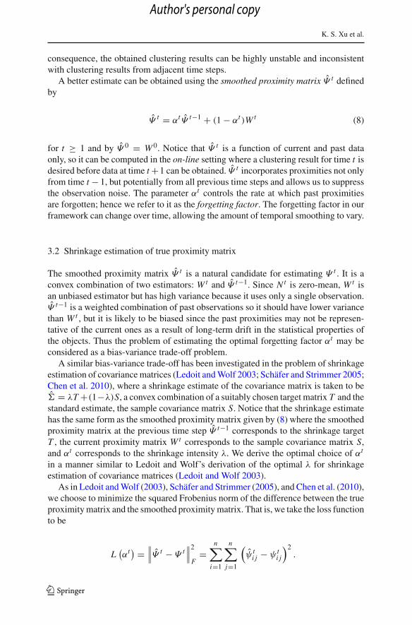
Fig. 7 Comparison of MSE in well-separated Gaussians experiment. The adaptively estimated forgettingfactor outperforms the constant forgetting factors and achieves MSE very close to the oracle forgettingfactor

0 10 20 30 400

0.2

0.4

0.6

0.8

1

Time step

αt Covariancechanged

Estimated αt

Oracle αt

(a) 40 samples

0 10 20 30 400

0.2

0.4

0.6

0.8

1

Time step

αt Covariancechanged

Estimated αt

Oracle αt

(b) 200 samples

Fig. 8 Comparison of oracle and estimated forgetting factors in well-separated Gaussians experiment. Thegap between the estimated and oracle forgetting factors decreases as the sample size increases

component memberships fixed, as described in Sect. 3.3. At time 19, we change thecovariance matrices to 0.3I to test how well the framework can respond to a suddenchange.

We run this experiment 100 times over 40 time steps using evolutionary k-meansclustering. The two clusters are well-separated so even static clustering is able tocorrectly identify them. However the tracking performance is improved significantlyby incorporating historical data, which can be seen in Fig. 7 where the MSE betweenthe estimated and true similarity matrices is plotted for several choices of forgettingfactor, including the estimated αt . We also compare to the oracle αt , which can becalculated using the true moments and cluster memberships of the data as shown inAppendix A.1 but is not implementable in a real application. Notice that the estimatedαt performs very well, and its MSE is very close to that of the oracle αt . The estimatedαt also outperforms all of the constant forgetting factors.

The estimated αt is plotted as a function of time in Fig. 8a. Since the clusters arewell-separated, only a single iteration is performed to estimate αt . Notice that boththe oracle and estimated forgetting factors quickly increase from 0 then level off toa nearly constant value until time 19 when the covariance matrix is changed. Afterthe transient due to the change in covariance, both the oracle and estimated forgettingfactors again level off. This behavior is to be expected because the two clusters are

123



Fig. 9 Setup of two collidingGaussians experiment: onecluster is slowly moved towardthe other, then a change incluster membership is simulated

−6 −4 −2 0 2 4 6−6

−4

−2

0

2

4

6

moving according to random walks. Notice that the estimated αt does not converge tothe same value the oracle αt appears to. This bias is due to the finite sample size. Theestimated and oracle forgetting factors are plotted in Fig. 8b for the same experimentbut with 200 samples rather than 40. The gap between the steady-state values ofthe estimated and oracle forgetting factors is much smaller now, and it continues todecrease as the sample size increases.

5.2 Two colliding Gaussians

The objective of this experiment is to test the effectiveness of the AFFECT frameworkwhen a cluster moves close enough to another cluster so that they overlap. We alsotest the ability of the framework to adapt to a change in cluster membership.

The setup of this experiment is illustrated in Fig. 9. We draw 40 samples from amixture of two 2-D Gaussian distributions, both with covariance matrix equal to iden-tity. The mixture proportion (the proportion of samples drawn from the second cluster)is initially chosen to be 1/2. The first cluster has mean (3, 3) and remains stationarythroughout the experiment. The second cluster’s mean is initially at (−3,−3) and ismoved toward the first cluster from time steps 0 to 9 by (0.4, 0.4) at each time. Attimes 10 and 11, we switch the mixture proportion to 3/8 and 1/4, respectively, tosimulate objects changing cluster. From time 12 onwards, both the cluster means andmixture proportion are unchanged. At each time, we draw a new sample.

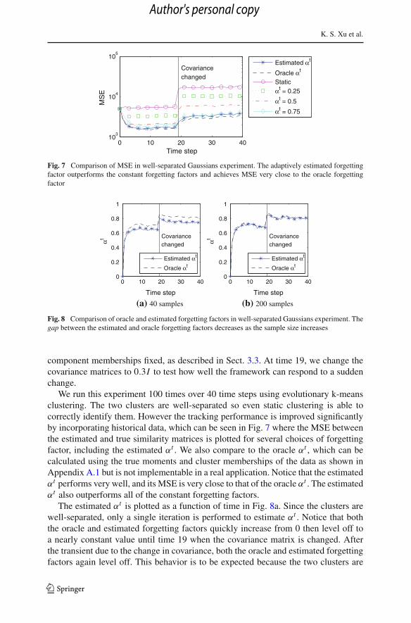
We run this experiment 100 times using evolutionary k-means clustering. The MSEin this experiment for varying αt is shown in Fig. 10. As before, the oracle αt iscalculated using the true moments and cluster memberships and is not implementablein practice. It can be seen that the choice of αt affects the MSE significantly. Theestimated αt performs the best, excluding the oracle αt , which is not implementable.Notice also that αt = 0.5 performs well before the change in cluster membershipsat time 10, i.e. when cluster 2 is moving, while αt = 0.75 performs better after thechange when both clusters are stationary.

The clustering accuracy for this experiment is plotted in Fig. 11. Since this exper-iment involves k-means clustering, we compare to the RG method. We simulate twofilter lengths for RG: a short-memory 3rd-order filter and a long-memory 10th-orderfilter. In Fig. 11 it can be seen that the estimated αt also performs best in Rand index,

123


K. S. Xu et al.

0 5 10 15 20 2510

3

104

105

106

Time step

MS

E

Change 1 Change 2

Estimated αt

Oracle αt

Static

αt = 0.25

αt = 0.5

αt = 0.75

Fig. 10 Comparison of MSE in two colliding Gaussians experiment. The estimated αt performs best bothbefore and after the change points

0 5 10 15 20 250.5

0.6

0.7

0.8

0.9

1

Time step

Ran

d in

dex

Change 1 Change 2

Estimated αt

Oracle αt

StaticRG (3rd order)RG (10th order)

Fig. 11 Comparison of Rand index in two colliding Gaussians experiment. The estimated αt detects thechanges in clusters quickly unlike the RG method

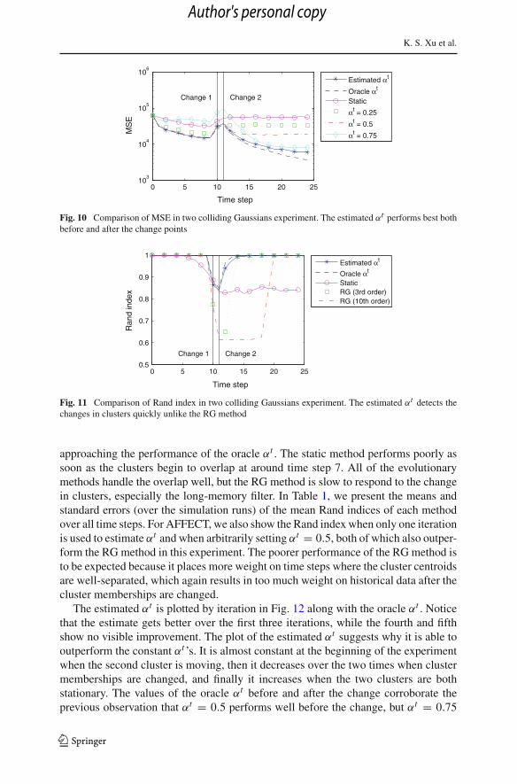
approaching the performance of the oracle αt . The static method performs poorly assoon as the clusters begin to overlap at around time step 7. All of the evolutionarymethods handle the overlap well, but the RG method is slow to respond to the changein clusters, especially the long-memory filter. In Table 1, we present the means andstandard errors (over the simulation runs) of the mean Rand indices of each methodover all time steps. For AFFECT, we also show the Rand index when only one iterationis used to estimate αt and when arbitrarily setting αt = 0.5, both of which also outper-form the RG method in this experiment. The poorer performance of the RG method isto be expected because it places more weight on time steps where the cluster centroidsare well-separated, which again results in too much weight on historical data after thecluster memberships are changed.

The estimated αt is plotted by iteration in Fig. 12 along with the oracle αt . Noticethat the estimate gets better over the first three iterations, while the fourth and fifthshow no visible improvement. The plot of the estimated αt suggests why it is able tooutperform the constant αt ’s. It is almost constant at the beginning of the experimentwhen the second cluster is moving, then it decreases over the two times when clustermemberships are changed, and finally it increases when the two clusters are bothstationary. The values of the oracle αt before and after the change corroborate theprevious observation that αt = 0.5 performs well before the change, but αt = 0.75

123



Table 1 Means and standarderrors of k-means Rand indicesin two colliding Gaussiansexperiment

Bolded number indicates bestperformer within one standarderror

Method Parameters Rand index

Static − 0.899 ± 0.002AFFECT Estimated αt (3 iterations) 0.984 ± 0.001

Estimated αt (1 iteration) 0.978 ± 0.001

αt = 0.5 0.975 ± 0.001

RG l = 3 0.955 ± 0.001

l = 10 0.861 ± 0.001

0 5 10 15 20 250

0.2

0.4

0.6

0.8

1

Time step

αt

Change 1 Change 2

1st iteration2nd iteration3rd iteration4th iteration5th iteration

Oracle αt

Fig. 12 Comparison of oracle and estimated forgetting factors in two colliding Gaussians experiment.There is no noticeable change after the third iteration

performs better afterwards. Notice that the estimated αt appears to converge to a lowervalue than the oracle αt . This is once again due to the finite-sample effect discussedin Sect. 5.1.

5.3 Flocks of boids

This experiment involves simulation of a natural phenomenon, namely the flockingbehavior of birds. To simulate this phenomenon we use the bird-oid objects (boids)model proposed by Reynolds (1987). The boids model allows us to simulate naturalmovements of objects and clusters. The behavior of the boids are governed by threemain rules:

1. Boids try to fly towards the average position (centroid) of local flock mates.2. Boids try to keep a small distance away from other boids.3. Boids try to fly towards the average heading of local flock mates.

Our implementation of the boids model is based on the pseudocode of Parker (2007).At each time step, we move each boid 1/100 of the way towards the average positionof local flock mates, double the distance between boids that are within 10 units of eachother, and move each boid 1/8 of the way towards the average heading.

We run two experiments using the boids model; one with a fixed number of flocksover time and one where the number of flocks varies over time.

123


K. S. Xu et al.

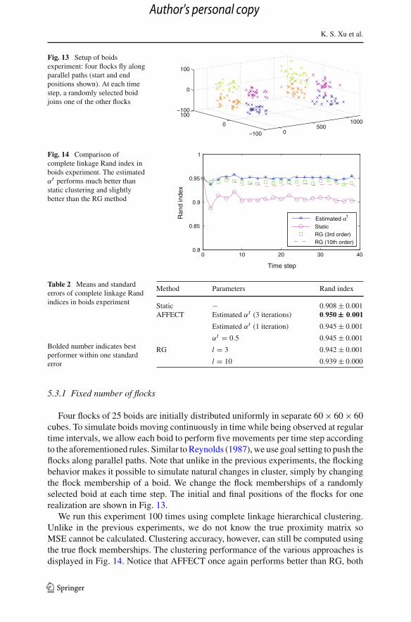
Fig. 13 Setup of boidsexperiment: four flocks fly alongparallel paths (start and endpositions shown). At each timestep, a randomly selected boidjoins one of the other flocks

0500

1000

−100

0

100−100

0

100

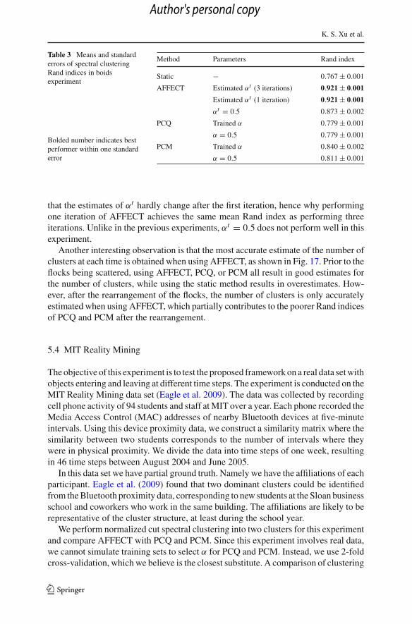
Fig. 14 Comparison ofcomplete linkage Rand index inboids experiment. The estimatedαt performs much better thanstatic clustering and slightlybetter than the RG method

0 10 20 30 400.8

0.85

0.9

0.95

1

Time step

Ran

d in

dex

Estimated αt

StaticRG (3rd order)RG (10th order)

Table 2 Means and standarderrors of complete linkage Randindices in boids experiment





αt = 0.5 0.945 ± 0.001

RG l = 3 0.942 ± 0.001

l = 10 0.939 ± 0.000

5.3.1 Fixed number of flocks

Four flocks of 25 boids are initially distributed uniformly in separate 60 × 60 × 60cubes. To simulate boids moving continuously in time while being observed at regulartime intervals, we allow each boid to perform five movements per time step accordingto the aforementioned rules. Similar to Reynolds (1987), we use goal setting to push theflocks along parallel paths. Note that unlike in the previous experiments, the flockingbehavior makes it possible to simulate natural changes in cluster, simply by changingthe flock membership of a boid. We change the flock memberships of a randomlyselected boid at each time step. The initial and final positions of the flocks for onerealization are shown in Fig. 13.

We run this experiment 100 times using complete linkage hierarchical clustering.Unlike in the previous experiments, we do not know the true proximity matrix soMSE cannot be calculated. Clustering accuracy, however, can still be computed usingthe true flock memberships. The clustering performance of the various approaches isdisplayed in Fig. 14. Notice that AFFECT once again performs better than RG, both

123



Fig. 15 Comparison of spectralclustering Rand index in boidsexperiment. The estimated αt

outperforms static clustering,PCQ, and PCM

0 10 20 30 400

0.2

0.4

0.6

0.8

1

Time step

Ran

d in

dex

Flocks scattered Flocks rearranged

Estimated αt

StaticPCQPCM

with short and long memory, although the difference is much smaller than in the twocolliding Gaussians experiment. The means and standard errors of the Rand indicesfor the various methods are listed in Table 2. Again, it can be seen that AFFECT is thebest performer. The estimated αt in this experiment is roughly constant at around 0.6.This is not a surprise because all movements in this experiment, including changes inclusters, are smooth as a result of the flocking motions of the boids. This also explainsthe good performance of simply choosing αt = 0.5 in this particular experiment.

5.3.2 Variable number of flocks

The difference between this second boids experiment and the first is that the number offlocks changes over time in this experiment. Up to time 16, this experiment is identicalto the previous one. At time 17, we simulate a scattering of the flocks by no longermoving them toward the average position of local flock mates as well as increasingthe distance at which boids repel each other to 20 units. The boids are then rearrangedat time 19 into two flocks rather than four.

We run this experiment 100 times. The RG framework cannot handle changes inthe number of clusters over time, thus we switch to normalized cut spectral clusteringand compare AFFECT to PCQ and PCM. The number of clusters at each time stepis estimated using the modularity criterion (Newman 2006). PCQ and PCM are notequipped with methods for selecting α. As a result, for each run of the experiment, wefirst performed a training run where the true flock memberships are used to computethe Rand index. The α which maximizes the Rand index is then used for the test run.

The clustering performance is shown in Fig. 15. The Rand indices for all methodsdrop after the flocks are scattered, which is to be expected. Shortly after the boidsare rearranged into two flocks, the Rand indices improve once again as the flocksseparate from each other. AFFECT once again outperforms the other methods, whichcan also be seen from the summary statistics presented in Table 3. The performanceof PCQ and PCM with both the trained α and arbitrarily chosen α = 0.5 are listed.Both outperform static clustering but perform noticeably worse than AFFECT withestimated αt . From Fig. 15, it can be seen that the estimated αt best responds to therearrangement of the flocks. The estimated forgetting factor by iteration is shown inFig. 16. Notice that the estimated αt drops when the flocks are scattered. Notice also

123


K. S. Xu et al.

Table 3 Means and standarderrors of spectral clusteringRand indices in boidsexperiment



Static − 0.767 ± 0.001

AFFECT Estimated αt (3 iterations) 0.921 ± 0.001


αt = 0.5 0.873 ± 0.002

PCQ Trained α 0.779 ± 0.001

α = 0.5 0.779 ± 0.001

PCM Trained α 0.840 ± 0.002

α = 0.5 0.811 ± 0.001

that the estimates of αt hardly change after the first iteration, hence why performingone iteration of AFFECT achieves the same mean Rand index as performing threeiterations. Unlike in the previous experiments, αt = 0.5 does not perform well in thisexperiment.

Another interesting observation is that the most accurate estimate of the number ofclusters at each time is obtained when using AFFECT, as shown in Fig. 17. Prior to theflocks being scattered, using AFFECT, PCQ, or PCM all result in good estimates forthe number of clusters, while using the static method results in overestimates. How-ever, after the rearrangement of the flocks, the number of clusters is only accuratelyestimated when using AFFECT, which partially contributes to the poorer Rand indicesof PCQ and PCM after the rearrangement.

5.4 MIT Reality Mining

The objective of this experiment is to test the proposed framework on a real data set withobjects entering and leaving at different time steps. The experiment is conducted on theMIT Reality Mining data set (Eagle et al. 2009). The data was collected by recordingcell phone activity of 94 students and staff at MIT over a year. Each phone recorded theMedia Access Control (MAC) addresses of nearby Bluetooth devices at five-minuteintervals. Using this device proximity data, we construct a similarity matrix where thesimilarity between two students corresponds to the number of intervals where theywere in physical proximity. We divide the data into time steps of one week, resultingin 46 time steps between August 2004 and June 2005.

In this data set we have partial ground truth. Namely we have the affiliations of eachparticipant. Eagle et al. (2009) found that two dominant clusters could be identifiedfrom the Bluetooth proximity data, corresponding to new students at the Sloan businessschool and coworkers who work in the same building. The affiliations are likely to berepresentative of the cluster structure, at least during the school year.

We perform normalized cut spectral clustering into two clusters for this experimentand compare AFFECT with PCQ and PCM. Since this experiment involves real data,we cannot simulate training sets to select α for PCQ and PCM. Instead, we use 2-foldcross-validation, which we believe is the closest substitute. A comparison of clustering

123



Fig. 16 Comparison ofestimated spectral clusteringforgetting factor by iteration inboids experiment. The estimatedforgetting factor drops at thechange point, i.e. when theflocks are scattered. There is nonoticeable change in theforgetting factor after the seconditeration

0 10 20 30 400

0.2

0.4

0.6

0.8

1

Time step

Est

imat

edαt


1st iteration2nd iteration3rd iteration

Fig. 17 Comparison of numberof clusters detected by spectralclustering in boids experiment.Using the estimated αt results inthe best estimates of the numberof flocks (4 before the changepoint and 2 after)

0 10 20 30 402

3

4

5

6

Time step

Det

ecte

d nu

mbe

r of

clu

ster

s


Estimated αt

StaticPCQPCM

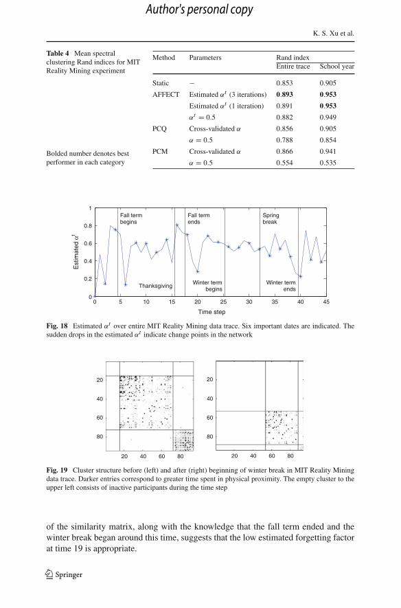
performance is given in Table 4. Both the mean Rand indices over the entire 46 weeksand only during the school year are listed. AFFECT is the best performer in bothcases. Surprisingly, PCQ barely performs better than static spectral clustering with thecross-validated α and even worse than static spectral clustering with α = 0.5. PCMfares better than PCQ with the cross-validated α but also performs worse than staticspectral clustering with α = 0.5. We believe this is due to the way PCQ and PCMsuboptimally handle objects entering and leaving at different time steps by estimatingprevious similarities and memberships, respectively. On the contrary, the method usedby AFFECT, described in Sect. 4.4.1, performs well even with objects entering andleaving over time.

The estimated αt is shown in Fig. 18. Six important dates are labeled. The start andend dates of the terms were taken from the MIT academic calendar (MIT–WWW 2005)to be the first and last day of classes, respectively. Notice that the estimated αt appearsto drop around several of these dates. These drops suggest that physical proximitieschanged around these dates, which is reasonable, especially for the students becausetheir physical proximities depend on their class schedules. For example, the similaritymatrices at time steps 18 and 19, before and after the beginning of winter break, areshown in Fig. 19. The detected clusters using the estimated αt are superimposed ontoboth matrices, with rows and columns permuted according to the clusters. Notice thatthe similarities, corresponding to time spent in physical proximity of other participants,are much lower at time 19, particularly in the smaller cluster. The change in the structure

123


K. S. Xu et al.

Table 4 Mean spectralclustering Rand indices for MITReality Mining experiment

Bolded number denotes bestperformer in each category

Method Parameters Rand indexEntire trace School year

Static − 0.853 0.905

AFFECT Estimated αt (3 iterations) 0.893 0.953

Estimated αt (1 iteration) 0.891 0.953

αt = 0.5 0.882 0.949

PCQ Cross-validated α 0.856 0.905

α = 0.5 0.788 0.854

PCM Cross-validated α 0.866 0.941

α = 0.5 0.554 0.535

0 5 10 15 20 25 30 35 40 450

0.2

0.4

0.6

0.8

1

Est

imat

edαt

Time step

Fall termbegins

Thanksgiving

Fall termends

Winter termbegins

Springbreak

Winter termends

Fig. 18 Estimated αt over entire MIT Reality Mining data trace. Six important dates are indicated. Thesudden drops in the estimated αt indicate change points in the network

20 40 60 80

20

40

60

80

20 40 60 80

20

40

60

80

Fig. 19 Cluster structure before (left) and after (right) beginning of winter break in MIT Reality Miningdata trace. Darker entries correspond to greater time spent in physical proximity. The empty cluster to theupper left consists of inactive participants during the time step

of the similarity matrix, along with the knowledge that the fall term ended and thewinter break began around this time, suggests that the low estimated forgetting factorat time 19 is appropriate.

123



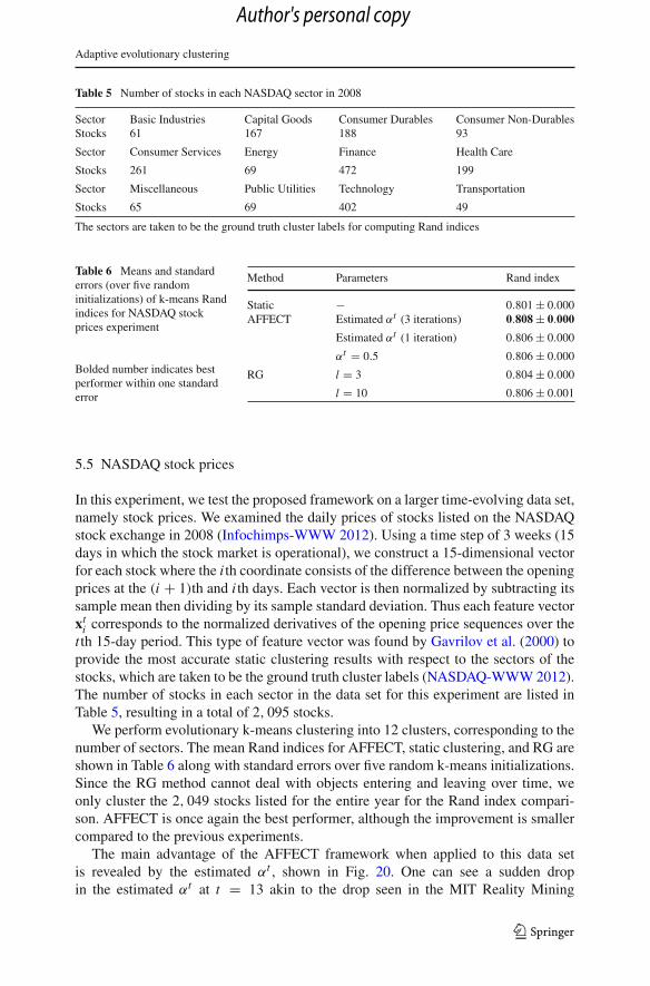
Table 5 Number of stocks in each NASDAQ sector in 2008

Sector Basic Industries Capital Goods Consumer Durables Consumer Non-DurablesStocks 61 167 188 93

Sector Consumer Services Energy Finance Health Care

Stocks 261 69 472 199

Sector Miscellaneous Public Utilities Technology Transportation

Stocks 65 69 402 49

The sectors are taken to be the ground truth cluster labels for computing Rand indices

Table 6 Means and standarderrors (over five randominitializations) of k-means Randindices for NASDAQ stockprices experiment





αt = 0.5 0.806 ± 0.000

RG l = 3 0.804 ± 0.000

l = 10 0.806 ± 0.001

5.5 NASDAQ stock prices

In this experiment, we test the proposed framework on a larger time-evolving data set,namely stock prices. We examined the daily prices of stocks listed on the NASDAQstock exchange in 2008 (Infochimps-WWW 2012). Using a time step of 3 weeks (15days in which the stock market is operational), we construct a 15-dimensional vectorfor each stock where the i th coordinate consists of the difference between the openingprices at the (i + 1)th and i th days. Each vector is then normalized by subtracting itssample mean then dividing by its sample standard deviation. Thus each feature vectorxt

i corresponds to the normalized derivatives of the opening price sequences over thet th 15-day period. This type of feature vector was found by Gavrilov et al. (2000) toprovide the most accurate static clustering results with respect to the sectors of thestocks, which are taken to be the ground truth cluster labels (NASDAQ-WWW 2012).The number of stocks in each sector in the data set for this experiment are listed inTable 5, resulting in a total of 2, 095 stocks.

We perform evolutionary k-means clustering into 12 clusters, corresponding to thenumber of sectors. The mean Rand indices for AFFECT, static clustering, and RG areshown in Table 6 along with standard errors over five random k-means initializations.Since the RG method cannot deal with objects entering and leaving over time, weonly cluster the 2, 049 stocks listed for the entire year for the Rand index compari-son. AFFECT is once again the best performer, although the improvement is smallercompared to the previous experiments.

The main advantage of the AFFECT framework when applied to this data setis revealed by the estimated αt , shown in Fig. 20. One can see a sudden dropin the estimated αt at t = 13 akin to the drop seen in the MIT Reality Mining

123


K. S. Xu et al.

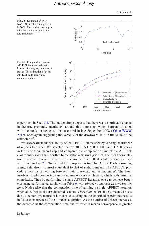
Fig. 20 Estimated αt overNASDAQ stock opening pricesin 2008. The sudden drop alignswith the stock market crash inlate September

0 5 10 150

0.2

0.4

0.6

0.8

1

Stock market crash

Time step

Est

imat

edαt

Fig. 21 Computation times ofAFFECT k-means and statick-means for varying numbers ofstocks. The estimation of αt inAFFECT adds hardly anycomputation time

0 500 1000 1500 2000 250010

−2

10−1

100

101

102

103

Number of stocks

Com

puta

tion

time

(sec

onds

)

Estimated αt (3 iterations)

Estimated αt (1 iteration)Static clustering3 × Static clustering

experiment in Sect. 5.4. The sudden drop suggests that there was a significant changein the true proximity matrix Ψ t around this time step, which happens to alignwith the stock market crash that occurred in late September 2008 (Yahoo-WWW2012), once again suggesting the veracity of the downward shift in the value of theestimated αt .

We also evaluate the scalability of the AFFECT framework by varying the numberof objects to cluster. We selected the top 100, 250, 500, 1, 000, and 1, 500 stocksin terms of their market cap and compared the computation time of the AFFECTevolutionary k-means algorithm to the static k-means algorithm. The mean computa-tion times over ten runs on a Linux machine with a 3.00 GHz Intel Xeon processorare shown in Fig. 21. Notice that the computation time for AFFECT when runninga single iteration is almost equivalent to that of static k-means. The AFFECT pro-cedure consists of iterating between static clustering and estimating αt . The latterinvolves simply computing sample moments over the clusters, which adds minimalcomplexity. Thus by performing a single AFFECT iteration, one can achieve betterclustering performance, as shown in Table 6, with almost no increase in computationtime. Notice also that the computation time of running a single AFFECT iterationwhen all 2, 095 stocks are clustered is actually less than that of static k-means. This isdue to the iterative nature of k-means; clustering on the smoothed proximities resultsin faster convergence of the k-means algorithm. As the number of objects increases,the decrease in the computation time due to faster k-means convergence is greater

123



than the increase due to estimating αt . The same observations apply for 3 iterations ofAFFECT when compared to 3 times the computation time for static clustering (labeledas “3 × static clustering”).

6 Conclusion

In this paper we proposed a novel adaptive framework for evolutionary clustering byperforming tracking followed by static clustering. The objective of the frameworkwas to accurately track the true proximity matrix at each time step. This was accom-plished using a recursive update with an adaptive forgetting factor that controlled theamount of weight to apply to historic data. We proposed a method for estimating theoptimal forgetting factor in order to minimize mean squared tracking error. The mainadvantages of our approach are its universality, allowing almost any static clusteringalgorithm to be extended to an evolutionary one, and that it provides an explicit methodfor selecting the forgetting factor, unlike existing methods. The proposed frameworkwas evaluated on several synthetic and real data sets and displayed good performancein tracking and clustering. It was able to outperform both static clustering algorithmsand existing evolutionary clustering algorithms.

There are many interesting avenues for future work. In the experiments presentedin this paper, the estimated forgetting factor appeared to converge after three itera-tions. We intend to investigate the convergence properties of this iterative process inthe future. In addition, we would like to improve the finite-sample behavior of theestimator. Finally, we plan to investigate other loss functions and models for the trueproximity matrix. We chose to optimize MSE and work with a block model in thispaper, but perhaps other functions or models may be more appropriate for certainapplications.

Acknowledgements We would like to thank the anonymous reviewers for their suggestions to improvethis article. Kevin Xu was partially supported by an award from the Natural Sciences and EngineeringResearch Council of Canada. This study was partially supported by the National Science Foundation GrantCCF 0830490 and the US Army Research Office Grant No. W911NF-09-1-0310.

Appendix

True similarity matrix for dynamic Gaussian mixture model

We derive the true similarity matrix Ψ and the matrix of variances of similaritiesvar(W ), where the similarity is taken to be the dot product, for data sampled from thedynamic Gaussian mixture model described in Sect. 3.3. These matrices are requiredin order to calculate the oracle forgetting factor for the experiments in Sects. 5.1 and5.2. We drop the superscript t to simplify the notation.

Consider two arbitrary objects xi ∼ N (µc, �c) and x j ∼ N (µd , �d) where theentries of µc and �c are denoted by μck and σckl , respectively. For any distinct i, jthe mean is

123


K. S. Xu et al.

E[xi xT

j

]=

p∑

k=1

E[xik x jk

] =p∑

k=1

μckμdk,

and the variance is

var(

xi xTj

)= E

[(xi xT

j

)2]

− E[xi xT

j

]2

=p∑

k=1

p∑

l=1

{E

[xik x jk xil x jl

] − μckμdkμclμdl}

=p∑

k=1

p∑

l=1

{(σckl + μckμcl) (σdkl + μdkμdl)− μckμdkμclμdl}

=p∑

k=1

p∑

l=1

{σcklσdkl + σcklμdkμdl + σdklμckμcl}

by independence of xi and x j . This holds both for xi , x j in the same cluster, i.e. c = d,and for xi , x j in different clusters, i.e. c �= d. Along the diagonal,

E[xi xT

i

]=

p∑

k=1

E[x2

ik

]=

p∑

k=1

(σckk + μ2

ck

).

The calculation for the variance is more involved. We first note that

E[x2

ik x2il

]= μ2

ckμ2cl + μ2

ckσcll + 4μckμclσckl + μ2clσckk + 2σ 2

ckl + σckkσcll ,

which can be derived from the characteristic function of the multivariate Gaussiandistribution (Anderson 2003). Thus

var(

xi xTi

)=

p∑

k=1

p∑

l=1

{E

[x2

ik x2il

]−

(σckk + μ2

ck

) (σcll + μ2

cl

)}

=p∑

k=1

p∑

l=1

{4μckμclσckl + 2σ 2

ckl

}.

The calculated means and variances are then substituted into (13) to compute theoracle forgetting factor. Since the expressions for the means and variances dependonly on the clusters and not any objects in particular, it is confirmed that both Ψ andvar(W ) do indeed possess the assumed block structure discussed in Sect. 3.3.

123



References

Ahmed A, Xing EP (2008) Dynamic non-parametric mixture models and the recurrent chinese restaurantprocess: with applications to evolutionary clustering. Proceedings of the SIAM international conferenceon data mining, Atlanta

Anderson TW (2003) An introduction to multivariate statistical analysis, 3rd edn. Wiley, HobokenBródka P, Saganowski S, Kazienko P (2012) GED: the method for group evolution discovery in social

networks. Soc Netw Anal Min. doi:10.1007/s13278-012-0058-8Carmi A, Septier F, Godsill SJ (2009) The Gaussian mixture MCMC particle algorithm for dynamic cluster

tracking. Proceedings of the 12th international conference on information fusion, SeattleChakrabarti D, Kumar R, Tomkins A (2006) Evolutionary clustering. Proceedings of the 12th ACM

SIGKDD international conference on knowledge discovery and data mining, PhiladelphiaCharikar M, Chekuri C, Feder T, Motwani R (2004) Incremental clustering and dynamic information

retrieval. SIAM J Comput 33(6):1417–1440Chen Y, Wiesel A, Eldar YC (2010) Shrinkage algorithms for MMSE covariance estimation. IEEE Trans

Signal Process 58(10):5016–5029Chi Y, Song X, Zhou D, Hino K, Tseng BL (2009) On evolutionary spectral clustering. ACM Trans Knowl

Discov Data 3(4):17Chung FRK (1997) Spectral graph theory. American Mathematical Society, ProvidenceEagle N, Pentland A, Lazer D (2009) Inferring friendship network structure by using mobile phone data.

Proc Nat Acad Sci 106(36):15274–15278Falkowski T, Bartelheimer J, Spiliopoulou M (2006) Mining and visualizing the evolution of subgroups

in social networks. Proceedings of the IEEE/WIC/ACM international conference on web intelligence,Hong Kong

Fenn DJ, Porter MA, McDonald M, Williams S, Johnson NF, Jones NS (2009) Dynamic communities inmultichannel data: an application to the foreign exchange market during the 2007–2008 credit crisis.Chaos 19(033):119

Gavrilov M, Anguelov D, Indyk P, Motwani R (2000) Mining the stock market: Which measure is best?Proceedings of 6th ACM SIGKDD international conference on knowledge discovery and data mining.ACM Press, New York, pp 487–496

Greene D, Doyle D, Cunningham P (2010) Tracking the evolution of communities in dynamic socialnetworks. Proceedings of international conference on advanced social network analysis and mining, pp176–183

Gretton A, Borgwardt KM, Rasch M, Schölkopf B, Smola AJ (2007) A kernel approach to comparingdistributions. Proceedings of the 22nd AAAI conference on artificial intelligence

Gupta C, Grossman R (2004) GenIc: a single pass generalized incremental algorithm for clustering. Pro-ceedings SIAM conference on data mining, Lake Buena Vista

Harvey AC (1989) Forecasting, structural time series models and the Kalman filter. Cambridge UniversityPress, Cambridge

Hastie T, Tibshirani R, Friedman J (2001) The elements of statistical learning: data mining, inference, andprediction. Springer, New York

Haykin S (2001) Kalman filtering and neural networks. Wiley-Interscience, New YorkHossain MS, Tadepalli S, Watson LT, Davidson I, Helm RF, Ramakrishnan N (2010) Unifying dependent

clustering and disparate clustering for non-homogeneous data. Proceedings of the 16th ACM SIGKDDinternational conference on knowledge discovery and data mining, pp 593–602

Infochimps-WWW (2012) NASDAQ Exchange Daily 1970–2010 Open, Close, High, Low and Vol-ume data set. http://www.infochimps.com/datasets/nasdaq-exchange-daily-1970-2010-open-close-high-low-and-volume

Ji X, Xu W (2006) Document clustering with prior knowledge. Proceedings of the 29th annual internationalACM SIGIR conference on research and development in information retrieval, New York, pp 405–412

Kuhn HW (1955) The Hungarian method for the assignment problem. Nav Res Logist Quart 2(1–2):83–97Ledoit O, Wolf M (2003) Improved estimation of the covariance matrix of stock returns with an application

to portfolio selection. J Empir Financ 10(5):603–621Li Y, Han J, Yang J (2004) Clustering moving objects. Proceedings of the 10th ACM SIGKDD international

conference on knowledge discovery and data miningLin YR, Chi Y, Zhu S, Sundaram H, Tseng BL (2009) Analyzing communities and their evolutions in

dynamic social networks. ACM Trans Knowl Discov Data 3(2):8

123


http://dx.doi.org/10.1007/s13278-012-0058-8

http://www.infochimps.com/datasets/nasdaq-exchange-daily-1970-2010-open-close-high-low-and-volume

http://www.infochimps.com/datasets/nasdaq-exchange-daily-1970-2010-open-close-high-low-and-volume

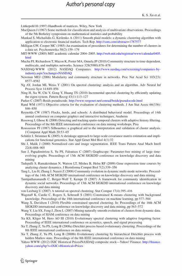
K. S. Xu et al.

Lütkepohl H (1997) Handbook of matrices. Wiley, New YorkMacQueen J (1967) Some methods for classification and analysis of multivariate observations. Proceedings

of the 5th Berkeley symposium on mathematical statistics and probabilityMankad S, Michailidis G, Kirilenko A (2011) Smooth plaid models: a dynamic clustering algorithm with

application to electronic financial markets. Tech Rep. http://ssrn.com/abstract=1787577Milligan GW, Cooper MC (1985) An examination of procedures for determining the number of clusters in

a data set. Psychometrika 50(2):159–179MIT-WWW (2005) MIT academic calendar 2004–2005. http://web.mit.edu/registrar/www/calendar0405.

htmlMucha PJ, Richardson T, Macon K, Porter MA, Onnela JP (2010) Community structure in time-dependent,

multiscale, and multiplex networks. Science 328(5980):876–878NASDAQ-WWW (2012) NASDAQ Companies. http://www.nasdaq.com/screening/companies-by-

industry.aspx?exchange=NASDAQNewman MEJ (2006) Modularity and community structure in networks. Proc Nat Acad Sci 103(23):

8577–8582Ng AY, Jordan MI, Weiss Y (2001) On spectral clustering: analysis and an algorithm. Adv Neural Inf

Process Syst 14:849–856Ning H, Xu W, Chi Y, Gong Y, Huang TS (2010) Incremental spectral clustering by efficiently updating

the eigen-system. Pattern Recog 43(1):113–127Parker C (2007) Boids pseudocode. http://www.vergenet.net/conrad/boids/pseudocode.htmlRand WM (1971) Objective criteria for the evaluation of clustering methods. J Am Stat Assoc 66(336):

846–850Reynolds CW (1987) Flocks, herds, and schools: A distributed behavioral model. Proceedings of 14th

annual conference on computer graphics and interactive techniques, AnaheimRosswog J, Ghose K (2008) Detecting and tracking spatio-temporal clusters with adaptive history filtering.

Proceedings of the 8th IEEE international conference on data mining workshops, PisaRousseeuw PJ (1987) Silhouettes: a graphical aid to the interpretation and validation of cluster analysis.

J Computat Appl Math 20:53–65Schäfer J, Strimmer K (2005) A shrinkage approach to large-scale covariance matrix estimation and impli-

cations for functional genomics. Stat Appl Genet Mol Biol 4(1):32Shi J, Malik J (2000) Normalized cuts and image segmentation. IEEE Trans Pattern Anal Mach Intell

22(8):888–905Sun J, Papadimitriou S, Yu PS, Faloutsos C (2007) Graphscope: Parameter-free mining of large time-

evolving graphs. Proceedings of 13th ACM SIGKDD conference on knowledge discovery and datamining

Tadepalli S, Ramakrishnan N, Watson LT, Mishra B, Helm RF (2009) Gene expression time courses byanalyzing cluster dynamics. J Bioinforma Comput Biol 7(2):339–356

Tang L, Liu H, Zhang J, Nazeri Z (2008) Community evolution in dynamic multi-mode networks. Proceed-ings of the 14th ACM SIGKDD international conference on knowledge discovery and data mining

Tantipathananandh C, Berger-Wolf T, Kempe D (2007) A framework for community identification indynamic social networks. Proceedings of 13th ACM SIGKDD international conference on knowledgediscovery and data mining

von Luxburg U (2007) A tutorial on spectral clustering. Stat Comput 17(4):395–416Wagstaff K, Cardie C, Rogers S, Schroedl S (2001) Constrained K-means clustering with background

knowledge. Proceedings of the 18th international conference on machine learning, pp 577–584Wang X, Davidson I (2010) Flexible constrained spectral clustering. In: Proceedings of the 16th ACM

SIGKDD international conference on knowledge discovery and data mining, pp 563–572Wang Y, Liu SX, Feng J, Zhou L (2007) Mining naturally smooth evolution of clusters from dynamic data.

Proceedings of SIAM conference on data miningXu KS, Kliger M, Hero AO III (2010) Evolutionary spectral clustering with adaptive forgetting factor.

Proceeding of IEEE international conference on acoustics, speech, and signal processingXu T, Zhang Z, Yu PS, Long B (2008a) Dirichlet process based evolutionary clustering. Proceedings of the

8th IEEE international conference on data miningXu T, Zhang Z, Yu PS, Long B (2008b) Evolutionary clustering by hierarchical Dirichlet process with

hidden Markov state. Proceedings of the 8th IEEE international conference on data miningYahoo-WWW (2012) IXIC Historical Prices|NASDAQ composite stock—Yahoo! Finance. http://finance.

yahoo.com/q/hp?s=IXIC+Historical+Prices

123


http://ssrn.com/abstract=1787577

http://web.mit.edu/registrar/www/calendar0405.html

http://web.mit.edu/registrar/www/calendar0405.html

http://www.nasdaq.com/screening/companies-by-industry.aspx?exchange=NASDAQ

http://www.nasdaq.com/screening/companies-by-industry.aspx?exchange=NASDAQ

http://www.vergenet.net/conrad/boids/pseudocode.html

http://finance.yahoo.com/q/hp?s=IXIC+Historical+Prices

http://finance.yahoo.com/q/hp?s=IXIC+Historical+Prices


Yang T, Chi Y, Zhu S, Gong Y, Jin R (2011) Detecting communities and their evolutions in dynamic socialnetworks—a Bayesian approach. Mach Learn 82(2):157–189

Zhang J, Song Y, Chen G, Zhang C (2009) On-line evolutionary exponential family mixture. Proceedingsof the 21st international joint conference on artificial intelligence, Pasadena

Zhang J, Song Y, Zhang C, Liu S (2010) Evolutionary hierarchical Dirichlet processes for multiple correlatedtime-varying corpora. Proceedings of the 16th ACM SIGKDD international conference on knowledgediscovery and data mining

123


web.eecs.umich.eduweb.eecs.umich.edu/~hero/Preprints/10.1007_s10618-012-0302-x.pdf · Adaptive...

Documents

Transcript of web.eecs.umich.eduweb.eecs.umich.edu/~hero/Preprints/10.1007_s10618-012-0302-x.pdf · Adaptive...