Web Crippling and Bending Moment Failure of Trapezoidal ... Web Crippling and Bending Moment Failure...
394
Combined web crippling and bending moment failure of first- generation trapezoidal steel sheeting : experiments, finite element models, mechanical models Citation for published version (APA): Hofmeyer, H. (2000). Combined web crippling and bending moment failure of first-generation trapezoidal steel sheeting : experiments, finite element models, mechanical models. Eindhoven: Technische Universiteit Eindhoven. https://doi.org/10.6100/IR540607 DOI: 10.6100/IR540607 Document status and date: Published: 01/01/2000 Document Version: Publisher’s PDF, also known as Version of Record (includes final page, issue and volume numbers) Please check the document version of this publication: • A submitted manuscript is the version of the article upon submission and before peer-review. There can be important differences between the submitted version and the official published version of record. People interested in the research are advised to contact the author for the final version of the publication, or visit the DOI to the publisher's website. • The final author version and the galley proof are versions of the publication after peer review. • The final published version features the final layout of the paper including the volume, issue and page numbers. Link to publication General rights Copyright and moral rights for the publications made accessible in the public portal are retained by the authors and/or other copyright owners and it is a condition of accessing publications that users recognise and abide by the legal requirements associated with these rights. • Users may download and print one copy of any publication from the public portal for the purpose of private study or research. • You may not further distribute the material or use it for any profit-making activity or commercial gain • You may freely distribute the URL identifying the publication in the public portal. If the publication is distributed under the terms of Article 25fa of the Dutch Copyright Act, indicated by the “Taverne” license above, please follow below link for the End User Agreement: www.tue.nl/taverne Take down policy If you believe that this document breaches copyright please contact us at: [email protected] providing details and we will investigate your claim. Download date: 16. Apr. 2020
Transcript of Web Crippling and Bending Moment Failure of Trapezoidal ... Web Crippling and Bending Moment Failure...

Combined web crippling and bending moment failure of first-generation trapezoidal steel sheeting : experiments, finiteelement models, mechanical modelsCitation for published version (APA):Hofmeyer, H. (2000). Combined web crippling and bending moment failure of first-generation trapezoidal steelsheeting : experiments, finite element models, mechanical models. Eindhoven: Technische UniversiteitEindhoven. https://doi.org/10.6100/IR540607
DOI:10.6100/IR540607
Document status and date:Published: 01/01/2000
Document Version:Publisher’s PDF, also known as Version of Record (includes final page, issue and volume numbers)
Please check the document version of this publication:
• A submitted manuscript is the version of the article upon submission and before peer-review. There can beimportant differences between the submitted version and the official published version of record. Peopleinterested in the research are advised to contact the author for the final version of the publication, or visit theDOI to the publisher's website.• The final author version and the galley proof are versions of the publication after peer review.• The final published version features the final layout of the paper including the volume, issue and pagenumbers.Link to publication
General rightsCopyright and moral rights for the publications made accessible in the public portal are retained by the authors and/or other copyright ownersand it is a condition of accessing publications that users recognise and abide by the legal requirements associated with these rights.
• Users may download and print one copy of any publication from the public portal for the purpose of private study or research. • You may not further distribute the material or use it for any profit-making activity or commercial gain • You may freely distribute the URL identifying the publication in the public portal.
If the publication is distributed under the terms of Article 25fa of the Dutch Copyright Act, indicated by the “Taverne” license above, pleasefollow below link for the End User Agreement:www.tue.nl/taverne
Take down policyIf you believe that this document breaches copyright please contact us at:[email protected] details and we will investigate your claim.
Download date: 16. Apr. 2020

Combined Web Crippling and Bending Moment Failure of First-Generation Trapezoidal Steel Sheeting
Experiments, Finite Element Models, Mechanical Models
H. Hofmeyer

ISBN 90-6814-114-7
H. Hofmeyer, 2000
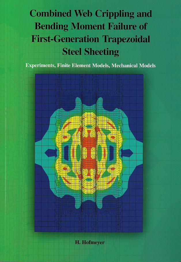
Cover: finite element simulation of experiment 17 (chapter 3), top view, Von Mises stresseson the outer shell element surface.
Printed by the Eindhoven University Press.
Combined Web Crippling and Bending Moment Failure of First-Generation Trapezoidal Steel Sheeting
Experiments, Finite Element Models, Mechanical Models
Proefschrift
ter verkrijging van de graad van doctor aan deTechnische Universiteit Eindhoven, op gezag van de
Rector Magnificus, prof.dr. M. Rem, voor een commissieaangewezen door het College voor Promoties in het
openbaar te verdedigen op maandag 18 december 2000om 16.00 uur door
Hèrm Hofmeyer
geboren te Beek (Limburg)

Dit proefschrift is goedgekeurd door de promotoren
prof.dr.ir. J.G.M. Kerstensenprof.ir. H.H. Snijder
Copromotor:dr.ir. M.C.M. Bakker
This research was supported by the Technology Foundation STW, applied science division ofNWO and the technology programme of the Ministry of Economic Affairs.

Overige leden kerncommissie:
Prof.ir. J.W.B. StarkProf. T. Peköz, Ph.D.Ir. A.W. Tomà
Overige leden promotiecommissie:
Prof.dr.ir. J. BlaauwendraadProf.ir. F. van HerwijnenProf.dr.ir. R.F.C. Kriens

Acknowledgements
I wish to express my gratitude to the following people:
J.G.M. Kerstens, H.H. Snijder, M.C.M. Bakker, J.W.B. Stark, A.W. Tomà, E. Ramm, M.Mahendran, H.L.M. Wijen, P.W.C. van Hoof, M.A.C.M. Ceelen, S. Ralston, J.P.W. Bongers,L.R.B. Tang, M.P.M.A. Limpens,
H. Hofmeyer, B.C. Hofmeyer-Van Doezelaar, E.A.C. Geurts van Kessel, and B. Hofmeyer.
Finally, I wish to express my gratitude to all those people, who have not been mentioned butcontributed in various ways to the successful completion of this thesis.
i
Contents
Notation .....................................................................................................................................v
1 Introduction ......................................................................................................................1
1.1 Trapezoidal Sheeting ....................................................................................................21.2 Problem definition ........................................................................................................6
1.2.1 Insight by current design rules................................................................................61.2.2 Accuracy of current design rules ............................................................................8
1.3 Research approach .......................................................................................................91.3.1 Experiments ............................................................................................................91.3.2 Finite element models.............................................................................................91.3.3 Mechanical models ...............................................................................................10
1.4 Preview of thesis contents ..........................................................................................11
2 Literature survey ............................................................................................................13
2.1 Existing design rules ...................................................................................................142.1.1 1996 AISI Cold-Formed Steel Specification (United States’ code).....................152.1.2 S136-94 Cold Formed Steel Structural Members (Canadian code) .....................192.1.3 ENV 1993-1-3 Eurocode3 - Part 1-3 (European code) ........................................202.1.4 Differences for the three design codes .................................................................212.1.5 Comparison of design codes.................................................................................222.1.6 Conclusions ..........................................................................................................26
2.2 Experimental work .....................................................................................................272.2.1 Pure concentrated load..........................................................................................272.2.2 Pure bending moment...........................................................................................282.2.3 Interaction.............................................................................................................29
2.3 Finite element models .................................................................................................312.4 Mechanical models .....................................................................................................342.5 Conclusions .................................................................................................................38
3 Experiments ....................................................................................................................39
3.1 Survey of sheeting use in practice .............................................................................413.1.1 Sheeting cross-section variables ...........................................................................413.1.2 Ratios between concentrated load and bending moment and η ratios .................42
3.2 Experiments ................................................................................................................473.2.1 Sheet sections .......................................................................................................473.2.2 Test rig..................................................................................................................503.2.3 Testing procedure .................................................................................................533.2.4 Test results ............................................................................................................54
ii
3.3 Post-failure modes ......................................................................................................563.3.1 Yield line patterns.................................................................................................563.3.2 Definition of post-failure modes...........................................................................583.3.3 Relevance rolling post-failure mode.....................................................................64
3.4 Conclusions .................................................................................................................65
4 Finite element models .....................................................................................................66
4.1 Model design ...............................................................................................................674.1.1 Mesh and elements ...............................................................................................684.1.2 Material properties................................................................................................704.1.3 Loading.................................................................................................................714.1.4 Boundary conditions.............................................................................................734.1.5 Solution.................................................................................................................744.1.6 Definitions ............................................................................................................744.1.7 Overview finite element models...........................................................................75
4.2 Results..........................................................................................................................764.2.1 Yield arc post-failure mode ..................................................................................764.2.2 Rolling post-failure mode.....................................................................................784.2.3 Yield eye post-failure mode .................................................................................814.2.4 Definition of ultimate failure modes ....................................................................85
4.3 Reliability of finite element models ...........................................................................874.3.1 Corner modelling and contact elements ...............................................................874.3.2 Difficulties for the yield eye post-failure mode....................................................87
4.4 Choice of correct finite element model .....................................................................914.4.1 Set of finite element simulations ..........................................................................914.4.2 Post-failure modes ................................................................................................934.4.3 Choice of correct finite element model ................................................................954.4.4 54-x-series, additional information.......................................................................954.4.5 25-x-series, additional information.......................................................................984.4.6 Equal ultimate loads and behaviour for yield arc and yield eye modes .............100
4.5 Conclusions ...............................................................................................................102
5 Ultimate failure mechanical model .............................................................................104
5.1 Development of the mechanical model ...................................................................1065.1.1 Introduction ........................................................................................................1065.1.2 Principle..............................................................................................................1075.1.3 Justification of the model ...................................................................................1085.1.4 Sensitivity of model............................................................................................1105.1.5 Model use (formulae) .........................................................................................110
5.2 Model versus experiments........................................................................................1155.2.1 Introduction ........................................................................................................1155.2.2 All selected experiments.....................................................................................1165.2.3 Tomà and Stark experiments ..............................................................................116
iii
5.2.4 Wing experiments...............................................................................................1175.2.5 Tsai experiments.................................................................................................1175.2.6 Experiments chapter 3 ........................................................................................118
5.3 Model behaviour for changing variables................................................................1195.3.1 Plate thickness ....................................................................................................1195.3.2 Web width...........................................................................................................1195.3.3 Yield strength .....................................................................................................1205.3.4 Span length .........................................................................................................1205.3.5 Bottom flange width ...........................................................................................1215.3.6 Angle between web and flange...........................................................................1215.3.7 Load-bearing plate width....................................................................................1225.3.8 Corner radius ......................................................................................................1235.3.9 η-ratio .................................................................................................................1235.3.10 M/Mu-ratio..........................................................................................................1245.3.11 Model results in interaction diagram..................................................................124
5.4 Conclusions ...............................................................................................................126
6 Post-failure modes ........................................................................................................127
6.1 Introduction ..............................................................................................................1286.1.1 Experiments chapter 3 ........................................................................................1286.1.2 Specific finite element models ...........................................................................1286.1.3 Post-failure mechanical models..........................................................................1286.1.4 Two aspects of successive post-failure modes ...................................................130
6.2 Mechanical model for the yield arc post-failure mode (MA1) .............................1316.2.1 Elastic behaviour ................................................................................................1316.2.2 Plastic behaviour.................................................................................................1316.2.3 Intersection of elastic and plastic curves ............................................................1326.2.4 Correction 1 of the ultimate load prediction.......................................................1336.2.5 Correction 2 of the ultimate load prediction.......................................................1336.2.6 Correction 3 of the ultimate load prediction.......................................................1346.2.7 Ultimate load Fu .................................................................................................1356.2.8 Yield line distance Lbf ........................................................................................1356.2.9 Summary.............................................................................................................135
6.3 Mechanical model for the rolling post-failure mode (MR1).................................1376.3.1 Elastic behaviour ................................................................................................1376.3.2 Plastic behaviour.................................................................................................1376.3.3 Intersection of elastic and plastic curves ............................................................1376.3.4 Corrections of the ultimate load prediction ........................................................1386.3.5 Summary.............................................................................................................138
6.4 Mechanical model for the yield eye post-failure mode (ME1)..............................1396.4.1 Elastic behaviour ................................................................................................1396.4.2 Plastic behaviour.................................................................................................1396.4.3 Intersection of elastic and plastic curves ............................................................1406.4.4 Cross-section deformation versus flip-disc deformation....................................1406.4.5 Load at section versus load at bottom flange .....................................................1406.4.6 Intersection of elastic and plastic curves ............................................................141
iv
6.5 Corner radius ............................................................................................................1436.6 Span length................................................................................................................1486.7 Angle between web and flange ................................................................................1516.8 Load-bearing plate width.........................................................................................1546.9 Bottom flange width .................................................................................................1576.10 Web width .............................................................................................................1596.11 Steel plate thickness..............................................................................................1616.12 Yield strength ........................................................................................................1626.13 Conclusions ...........................................................................................................163
7 Conclusions and recommendations.............................................................................164
7.1 Conclusions ...............................................................................................................1657.1.1 Research aim.......................................................................................................1657.1.2 Results achieved .................................................................................................1657.1.3 Scientific contribution ........................................................................................1657.1.4 Contribution to practice ......................................................................................166
7.2 Future research, recommendations ........................................................................1677.2.1 Better cross-section models ................................................................................1677.2.2 Simplification ultimate failure mechanical model..............................................1677.2.3 Modern sheeting .................................................................................................1677.2.4 Fitting of the mechanical models........................................................................167
Literature ..............................................................................................................................168
A Appendix experiments..................................................................................................175
Summary ...............................................................................................................................183

v
Notation
Design rules and general variables
b1,2 Effective widths of web parts under compression and tension [mm].bbf;eff Effective bottom flange width [mm].bw;eff Effective web width [mm].c, d Values for interaction rule. Are found by curve-fitting.F Actual concentrated load [N].f1,2 Maximum compression and tension stresses in the web [N/mm2].fbf Normal stress in bottom flange [N/mm2].fi Functions for ultimate concentrated load design rule.h1, h2 Variables to illustrate the web crippling deformation ∆hw [mm].k Web crippling stiffness, ratio between concentrated load and web crippling
deformation [N/mm].M Actual bending moment [Nmm].Mu Ultimate bending moment if there is no concentrated load [Nmm].pi, qi Parameters for ultimate concentrated load design rule. Are found by curve fitting.Ru Ultimate concentrated load if there is no bending moment [N].vi Sheeting variables for ultimate concentrated load design rule.∆hw Web crippling deformation. The reduction of height hw [mm].α Additional variables for the Eurocode3 design code.δ ... Incremental ...λ1, λ2, Cy Additional variables for the AISI design code.ρ, λ, k Additional variables for the AISI design code.ψ Ratio between stresses f1 and f2.
Sheeting variables (see also figure 2-3, chapter 2)
bbf Bottom flange width, measured between the points of intersection of the web andflange midlines [mm].
bbffl Flat bottom flange width [mm]. Also possible is bbf;fl.bm Sheet section width [mm].btf Top flange width, measured between the points of intersection of the web and
flange midlines [mm].btffl Flat top flange width [mm]. Also possible is btf;fl.bw Web width, measured between the points of intersection of the web and flange
midlines [mm].bwfl Flat web width [mm]. Also possible is bw;fl.E Modulus of elasticity [N/mm2].fy Steel yield strength [N/mm2].hm Sheeting height between top and bottom flange midlines [mm].hw Sheeting height between top of top flange and bottom of bottom flange [mm].Llb Load bearing plate width [mm].Lspan Span length [mm]. Also possible is Lsp.rbf Radius of bottom corner midline [mm].ribf Interior radius of bottom corner [mm].ritf Interior radius of top corner [mm].
vi
rtf Radius of top corner midline [mm].t Steel plate thickness [mm].θw Angle between web and flange [deg.].
Yield line distances
Lbf;left;edgeLbf;right;edge
Distance between left / right two yield lines in bottom flange at the bottom corner[mm].
Lbf;left;inLbf;right;in
Distance between load-bearing plate and inner left / right yield line in bottomflange [mm].
Lbf;left;outLbf;right;out
Distance between load-bearing plate and outer left / right yield line in bottomflange [mm].
Ltf Distance between support and yield line in top flange [mm].Lw Distance between bottom corner and yield line in web [mm].Lyb Distance between yield lines in bottom flange (Bakker's model) [mm].Lyt Distance between yield lines in top flange (Bakker's model) [mm].
Experiments
a, b, c Variables to illustrate measured versus real web crippling deformation [mm].A, R, E Yield arc, rolling, and yield eye post-failure modes.A>E A yield arc post-failure mde is followed by a yield eye post-failure mode.A>R A yield arc post-failure mode is followed by a rolling post-failure mode.Fimec Mechanism / mode initiation load [N].Ftest Ultimate load Fu measured during an experiment [N].q Equally distributed load [N/mm2].w Beam deflection [mm].η Equals M/Mu divided by F/Ru.ϕ Support rotation [rad.].
Finite element models
a Distance between strips [mm].d1, d2 Displacements to illustrate loading and behaviour for different post-failure modes.Fi, Fj, di, dj Forces [N] and distances [mm] to illustrate the concept of contact elements.i, i', k, k' Node locations to illustrate the concept of contact elements.rotx, roty, rotz Rotations around the x-, y-, and z-axes.ux, uy, uz Displacements along the x-, y-, and z-axes.x, y, z Variables for coordinate system.εe Engineering strain.εr Real strain.σe Engineering stress [N/mm2].σr Real stress [N/mm2].
vii
Ultimate failure mechanical model
b Abbreviated variable. Stands for bbffl [mm].dQ, dP Distances of point Q and P to line of intersection top flange and web [mm].f1 Function.Fbf Compressive force in bottom flange [N].h1, h2 Variables to illustrate the web crippling deformation ∆hw [mm].I Moment of inertia of area in sheeting longitudinal direction for sheeting part
above the load-bearing plate [mm4].Is Moment of inertia of area for complete sheeting cross-section [mm4].Ma Bending moment in sheeting part above the load-bearing plate [Nmm].P, Q, R, S Points at the bottom flange.Rh Reaction force for sheeting part above the load bearing plate [N].w0 Out-of-plane displacement of modelled part bottom flange [mm].wP, wR, wS Out-of-plane displacements of point P, R, and S [mm].y0 Initial imperfection of midpoint in modelled part of bottom flange [mm].zp Distance between centre of gravity and bottom flange [mm].∆dQ, ∆dP Reduction of distances dQ, dP [mm].α, β, b Substitution variables.λ, L, C1, C2,C3, D, p
Substitution variables.
ν Poisson's ratio (0.3).σVM Von Mises stress [N/mm2].σx max, z max Normal stresses in the outer fibres caused by bending moment in direction of x/z-
axis [N/mm2].σx,z Normal stress in direction of x/z-axis [N/mm2].σz Compressive normal stress in bottom flange [N/mm2].τxz Shear stress in plane perpendicular to the x-axis, in z-direction [N/mm2].
Post-failure mechanical models
a Length of yield eye / flip disc [mm].A, B, C Constants.b Width of yield eye / flip disc [mm].dx Infinite small piece of sheeting in length direction.F2p Load to deform two parts adjacent to the load-bearing plate [N].Fcs Load to deform cross-section [N].Fcsu Ultimate load of cross-section [N].Fe Load to deform cross-section elastically [N].Fl Extra force due to the indentation of the cross-section [N].fl1,2 Length factor 1, 2.Fp Load to deform cross-section plastically [N].Fylbf Load to form yield lines in the bottom flange [N].Me External bending moment [Nmm].s Distance from neutral axis to outer fibre of bottom flange [mm].ua, ub Movements of yield lines in the cross-section [mm].x, α, β Substituting variables.∆ Out-of-plane deflection yield eye / flip disc [mm].

viii
∆bwfl Reduction of distance bwfl [mm].δEe1 Incremental external energy cross-section only.δEe2 Incremental external energy cross-section and sheet section deflection.ϕa, ϕb, ϕc Rotations of yield lines in the cross-section [rad.].ϕd, ϕe Rotations of yield lines in the longitudinal section [rad.].

1
1 Introduction
Chapter abstractCold-formed trapezoidal sheeting of thin steel plate is introduced. Problems with currentdesign rules for this sheeting are shown. It is explained how the research presented in thisthesis tries to solve these problems. Finally, the thesis contents are outlined.
2
1.1 Trapezoidal Sheeting
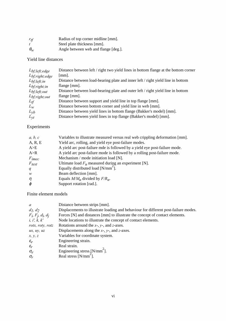
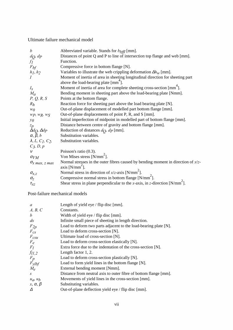
Cold-formed trapezoidal sheeting of thin steel plate is a very popular product for buildingconstruction. It combines low weight and high strength and is economical in use. Figures 1-1and 1-2 show photos of sheeting used as cladding and for roof construction.
Figure 1-1. Sheeting used as cladding (and as a corrugated shelter).
Figure 1-2. Sheeting used for roof construction.
3
ManufacturingSteel is cast continuously into a long steel strip after which the long steel strip is cut intosmaller pieces. The pieces are, while they are 1250o C., rolled into moderate thick steel plate(2 to 3 mm). The moderate thick steel plate is cold rolled into thin steel plate (0.5-1.5 mm).This thin steel plate is heated to remove residual stresses. Then, the thin steel plate is coldrolled again to obtain the requested yield strength. Finally, the thin steel plate will often becoated by a thin layer of zinc. There are three different methods for transforming the thin steelplate into profiled sections like trapezoidal sheeting: cold roll forming, press brake operation,and bending brake operation [Yuww85a]. Trapezoidal sheeting is usually made via cold rollforming. In recent decades, new generations of sheeting have been made by using profiledrolls for cold roll forming.
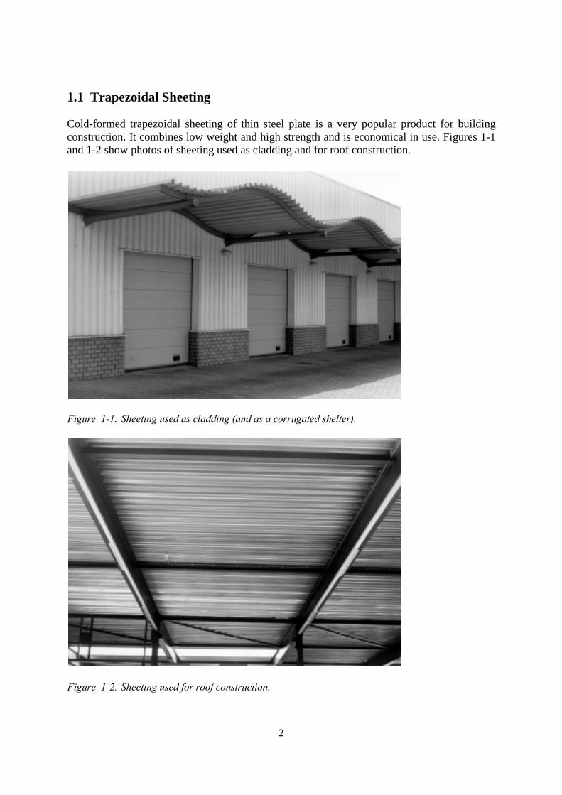
Three generations of sheetingFigure 1-3 shows three generations of sheeting. First generation sheeting is a rolled platewithout any stiffeners. Second generation sheeting has stiffeners in the longitudinal directiononly. Third generation sheeting also has stiffeners in the transverse direction.
First generation sheeting(unstiffened)
Second generation sheeting(longitudinally stiffened)
Third generation sheeting(longitudinally and transverselystiffened)
Figure 1-3. Generations of sheeting.
In this thesis, only first generation sheeting is investigated, although second and thirdgeneration sheetings are widely used. The reason for this limitation is that it is important tofirst understand the behaviour of the relatively simple first generation sheeting.
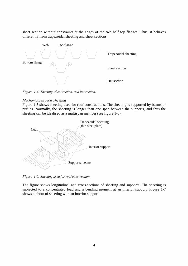
DefinitionsNext to trapezoidal sheeting, sheet sections and hat sections will be introduced later in thisthesis. Here, only their definitions are given (see figure 1-4). Trapezoidal sheeting is folded(rolled) plate with several webs and flanges. A sheet section is a combination of one bottomflange, two webs, and two half top flanges. Constraints are applied at the edges of the two halftop flanges to let this sheet section behave like infinitely wide sheeting. A hat section is a
4
sheet section without constraints at the edges of the two half top flanges. Thus, it behavesdifferently from trapezoidal sheeting and sheet sections.
Trapezoidal sheeting
Sheet section
Hat section
Bottom flange
Top flangeWeb
Figure 1-4. Sheeting, sheet section, and hat section.
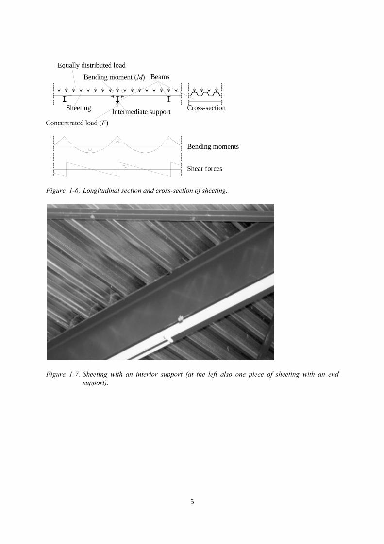
Mechanical aspects sheetingFigure 1-5 shows sheeting used for roof constructions. The sheeting is supported by beams orpurlins. Normally, the sheeting is longer than one span between the supports, and thus thesheeting can be idealised as a multispan member (see figure 1-6).
Supports: beams
Trapezoidal sheeting(thin steel plate)
Interior support
Load
Figure 1-5. Sheeting used for roof construction.
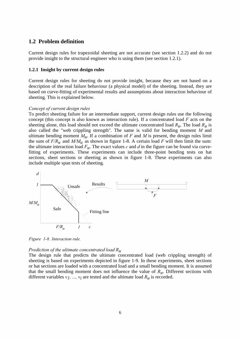
The figure shows longitudinal and cross-sections of sheeting and supports. The sheeting issubjected to a concentrated load and a bending moment at an interior support. Figure 1-7shows a photo of sheeting with an interior support.
5
Sheeting
Beams
Intermediate support
Equally distributed load
Cross-section
Bending moment (M)
Concentrated load (F)
Bending moments
Shear forces
Figure 1-6. Longitudinal section and cross-section of sheeting.
Figure 1-7. Sheeting with an interior support (at the left also one piece of sheeting with an endsupport).
6
1.2 Problem definition
Current design rules for trapezoidal sheeting are not accurate (see section 1.2.2) and do notprovide insight to the structural engineer who is using them (see section 1.2.1).
1.2.1 Insight by current design rules
Current design rules for sheeting do not provide insight, because they are not based on adescription of the real failure behaviour (a physical model) of the sheeting. Instead, they arebased on curve-fitting of experimental results and assumptions about interaction behaviour ofsheeting. This is explained below.
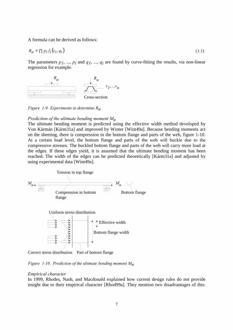
Concept of current design rulesTo predict sheeting failure for an intermediate support, current design rules use the followingconcept (this concept is also known as interaction rule). If a concentrated load F acts on thesheeting alone, this load should not exceed the ultimate concentrated load Ru. The load Ru isalso called the "web crippling strength". The same is valid for bending moment M andultimate bending moment Mu. If a combination of F and M is present, the design rules limitthe sum of F/Ru and M/Mu as shown in figure 1-8. A certain load F will then limit the sum:the ultimate interaction load Fu. The exact values c and d in the figure can be found via curve-fitting of experiments. These experiments can include three-point bending tests on hatsections, sheet sections or sheeting as shown in figure 1-8. These experiments can alsoinclude multiple span tests of sheeting.
M/Mu
F/Ru 1
1
d
c
Safe
Unsafe
F
MResults
Fitting line
Figure 1-8. Interaction rule.
Prediction of the ultimate concentrated load RuThe design rule that predicts the ultimate concentrated load (web crippling strength) ofsheeting is based on experiments depicted in figure 1-9. In these experiments, sheet sectionsor hat sections are loaded with a concentrated load and a small bending moment. It is assumedthat the small bending moment does not influence the value of Ru. Different sections withdifferent variables v1, ..., vi are tested and the ultimate load Ru is recorded.
7
A formula can be derived as follows:
( )∏= iqivifipuR , (1.1)
The parameters p1, ..., pi and q1, ..., qi are found by curve-fitting the results, via non-linearregression for example.
v1,...,vn
Cross-section
RuRu
Figure 1-9. Experiments to determine Ru.
Prediction of the ultimate bending moment MuThe ultimate bending moment is predicted using the effective width method developed byVon Kármán [Kárm31a] and improved by Winter [Wint49a]. Because bending moments acton the sheeting, there is compression in the bottom flange and parts of the web, figure 1-10.At a certain load level, the bottom flange and parts of the web will buckle due to thecompressive stresses. The buckled bottom flange and parts of the web will carry more load atthe edges. If these edges yield, it is assumed that the ultimate bending moment has beenreached. The width of the edges can be predicted theoretically [Kárm31a] and adjusted byusing experimental data [Wint49a].
Mu Mu
Compression in bottom flange
Tension in top flange
Part of bottom flangeCorrect stress distribution
Uniform stress distribution
Bottom flange width
Effective width
Bottom flange
Figure 1-10. Prediction of the ultimate bending moment Mu.
Empirical characterIn 1999, Rhodes, Nash, and Macdonald explained how current design rules do not provideinsight due to their empirical character [Rhod99a]. They mention two disadvantages of this:

8
"... (i) the rules are strictly confined to the range for which they have been proven, and (ii) it isoften difficult to ascertain the engineering reasoning behind the different parts of the rathercomplex equations ...".
1.2.2 Accuracy of current design rules
The previous section showed that the current design rules have three parts: a calculation forthe ultimate concentrated load Ru only (web crippling), a calculation for the ultimate bendingmoment Mu, and the interaction rule for finding the ultimate interaction load Fu. In thissection, we will discuss why design rules are not accurate because all investigated designcodes give different results for the same experiments, for all three parts of the design rules.This is explained in chapter 2, section 2.1.5. The conclusions of this section are given below.
For the ultimate concentrated load Ru, predictions of the three design codes investigated candiffer between +18 and -58 %.
The three design codes use the same concept for predicting the ultimate concentrated load Mu.However, due to small differences in formulae and restrictions, predictions can differ between-20 and 20 %.
The three design codes use the same concept for predicting the ultimate interaction load Fu.However, due to different numerical values in the formulae, there are differences between -40% and 10 %.
Findings in literatureDavies and Jiang [Davi97a] carried out finite element calculations to test two typicaltrapezoidal types of sheeting for different ratios between the bending moment M andconcentrated load F. "The computational results reveal that M/Mu can be significantly greaterthan 1 (note that 1 is the design rule limit) when F/Ru is less than 0.4*. A possible explanationfor this increase in strength is that the interaction of bending moment and reaction causes acomplicated stress combination in the sheeting".
* For small concentrated loads, the design rules only calculate the ultimate bending moment.
9
1.3 Research approach
The problem definition in section 1.2 showed that current design rules for sheeting are notaccurate and do not provide the structural engineer with any insight. To develop better designrules, which are accurate and provide insight, the following research approach is followed.The concepts of the current design rules and the interaction rule are discarded. Instead of this,the failure behaviour of sheeting for practical loading situations is described.
To this purpose, experiments were carried out on sheet sections to investigate the behaviourof trapezoidal sheeting. Following that, mechanical models were developed. Thesemechanical models predict the ultimate load and describe the physical phenomena that occur(thus providing insight). The mechanical models can be used as a basis for new design rules.Finite element models were used in the evaluation of the experiments and the development ofmechanical models.
1.3.1 Experiments
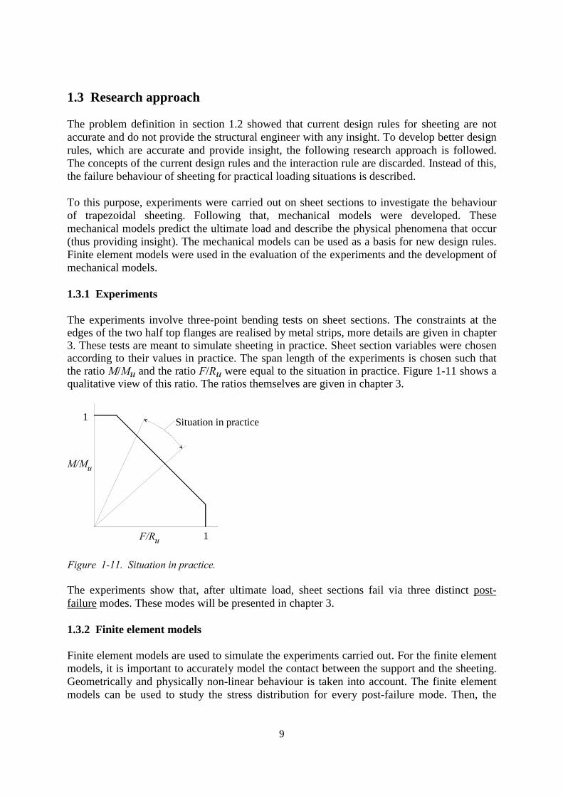
The experiments involve three-point bending tests on sheet sections. The constraints at theedges of the two half top flanges are realised by metal strips, more details are given in chapter3. These tests are meant to simulate sheeting in practice. Sheet section variables were chosenaccording to their values in practice. The span length of the experiments is chosen such thatthe ratio M/Mu and the ratio F/Ru were equal to the situation in practice. Figure 1-11 shows aqualitative view of this ratio. The ratios themselves are given in chapter 3.
1
1 Situation in practice
F/Ru
M/Mu
Figure 1-11. Situation in practice.
The experiments show that, after ultimate load, sheet sections fail via three distinct post-failure modes. These modes will be presented in chapter 3.
1.3.2 Finite element models
Finite element models are used to simulate the experiments carried out. For the finite elementmodels, it is important to accurately model the contact between the support and the sheeting.Geometrically and physically non-linear behaviour is taken into account. The finite elementmodels can be used to study the stress distribution for every post-failure mode. Then, the

10
finite element models show that, until and at ultimate load, sheet sections have two distinctultimate failure modes. Note that experiments showed three post-failure modes after ultimateload. Ultimate failure modes cannot be distinguished for the experiments.
1.3.3 Mechanical models
In this thesis, a mechanical model is defined as a set of formulae. The formulae representphysical phenomena like deformations, stresses, yield lines, and geometry. These physicalphenomena are used to model the physical behaviour of the sheeting. A mechanical model isdifferent from a finite element model: the formulae of a mechanical model use only variablesthat directly describe the sheeting geometry like web height, corner radius, etc. The formulaeof a finite element model mainly describe equilibrium for many very small parts of thesheeting.
Prediction of the ultimate loadFinite element calculations showed that until and at ultimate load, sheet sections fail by twodifferent ultimate failure modes. One of these ultimate failure modes is not relevant forpractice because it only occurs for large sheet section corner radii and (impractical) smallsupport widths. This will be shown in chapter 3. For the remaining ultimate failure mode, amodel was developed. This model predicts the ultimate load by finding the loadcorresponding to the occurrence of first yielding in the sheet section. The model providesinsight into the behaviour until and at ultimate load, because it is based on the physicalbehaviour of the sheet section.
Insight into post-failure modesTo develop additional insight into the occurrence of the three post-failure modes (as shown bythe experiments) after ultimate load, several post-failure mechanical models were developed.These models predict ultimate load via the intersection of an elastic and plastic loaddeformation curve. The plastic curves are different for each post-failure mode, while theelastic load deformation curves are identical.
11
1.4 Preview of thesis contents
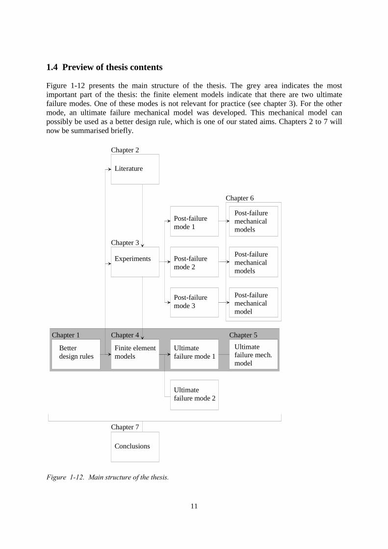
Figure 1-12 presents the main structure of the thesis. The grey area indicates the mostimportant part of the thesis: the finite element models indicate that there are two ultimatefailure modes. One of these modes is not relevant for practice (see chapter 3). For the othermode, an ultimate failure mechanical model was developed. This mechanical model canpossibly be used as a better design rule, which is one of our stated aims. Chapters 2 to 7 willnow be summarised briefly.
Betterdesign rules
Literature
Experiments
Finite elementmodels
Ultimatefailure mode 1
Ultimatefailure mode 2
Ultimatefailure mech.model
Post-failuremode 1
Post-failuremode 2
Post-failuremode 3
Post-failure mechanicalmodels
Conclusions
Chapter 1
Chapter 2
Chapter 3
Chapter 4 Chapter 5
Chapter 6
Chapter 7
Post-failure mechanicalmodels
Post-failure mechanicalmodel
Figure 1-12. Main structure of the thesis.
12
Chapter 2, literature surveyChapter 2 presents research carried out in the past that is relevant for this thesis. Threecurrently used design codes will be compared.
Chapter 3, experimentsTo develop mechanical models, experiments had to be carried out to study sheetingbehaviour. The experimental research is presented in chapter 3. The chapter starts with asurvey on how sheeting is used in practice. Then, the experiments themselves are presented.Detailed experimental data are presented in an appendix. The experiments show three post-failure modes after ultimate load.
Chapter 4, finite element modelsIn chapter 4, the finite element models are used to simulate the three post-failure modes foundfor the experiments. The finite elements models show that until and at ultimate load, there areonly two ultimate failure modes.
Chapter 5, ultimate failure mechanical modelAlthough the finite element models show two ultimate failure modes, only one of these modesis relevant for practice. In chapter 5, an ultimate failure mechanical model for this ultimatefailure mode is presented. The model is compared with the experiments in this thesis, but alsowith experiments found in literature. The model performs well and provides the structuralengineer with insight. Thus, it can possibly be used in future as a candidate design rule.
Chapter 6, post-failure modesChapter 6 presents several post-failure mechanical models for all three post-failure modes.Using these models, it can be investigated which post-failure mode occurs if sheetingvariables change. And although these models are not meant to be a basis for new design rules,they do improve insight into sheeting behaviour.
Chapter 7, conclusions and recommendationsChapter 7 presents the conclusions and recommendations for further research in this field.

13
2 Literature survey
Chapter abstractCurrent design rules for failure of sheeting at an interior support are all based on the sameconcept: sheeting can fail by concentrated load only, by bending moment only, and byinteraction of concentrated load and bending moment. Existing experiments on sheeting, sheetsections, or hat sections do not provide detailed information about failure modes. Finiteelement models that model sheeting behaviour often neglect to model the corner radii and arerarely aiming at increasing the knowledge on sheeting behaviour. There is only one fullymechanical model in literature for sheeting in the practical range of concentrated load andbending moment.
14
2.1 Existing design rules
In the world, there are many design codes for sheeting capacity, so it is impossible to presentthem all here. However, as far as the author knows, all current design codes use the sameconcept to predict sheeting failure, as explained in the introduction. Three current designcodes, which contain design rules for sheeting capacity, will be presented here. The code usedin the United States of America [Aisi96a], the code used in Europe [Euro96a], and the codeused in Canada [Cana95a]. The first two codes have been selected because together they servethe largest part of the market for sheeting. The Canadian code has proved to be accurate forpredicting the ultimate concentrated load [Bakk86a].
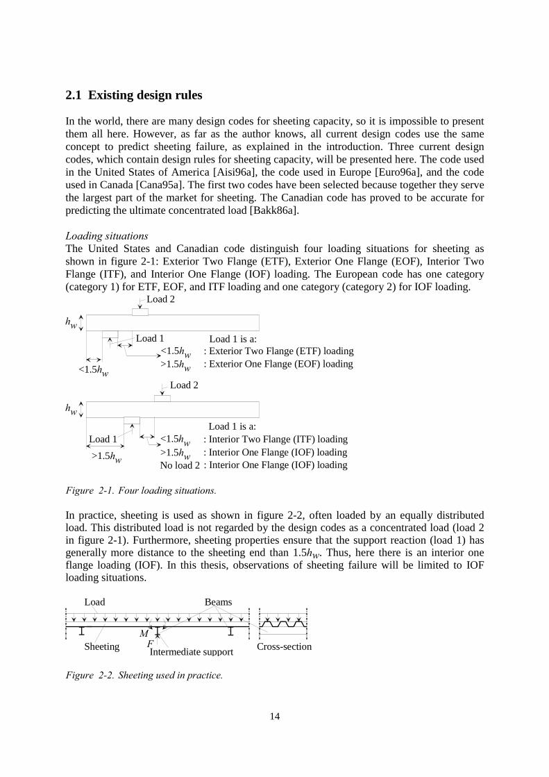
Loading situationsThe United States and Canadian code distinguish four loading situations for sheeting asshown in figure 2-1: Exterior Two Flange (ETF), Exterior One Flange (EOF), Interior TwoFlange (ITF), and Interior One Flange (IOF) loading. The European code has one category(category 1) for ETF, EOF, and ITF loading and one category (category 2) for IOF loading.
<1.5hw
hw
<1.5hw : Exterior Two Flange (ETF) loading>1.5hw : Exterior One Flange (EOF) loading
>1.5hw
hw
<1.5hw : Interior Two Flange (ITF) loading>1.5hw : Interior One Flange (IOF) loading
Load 2
Load 1Load 1 is a:
No load 2 : Interior One Flange (IOF) loading
Load 1 is a:
Load 2
Load 1
Figure 2-1. Four loading situations.
In practice, sheeting is used as shown in figure 2-2, often loaded by an equally distributedload. This distributed load is not regarded by the design codes as a concentrated load (load 2in figure 2-1). Furthermore, sheeting properties ensure that the support reaction (load 1) hasgenerally more distance to the sheeting end than 1.5hw. Thus, here there is an interior oneflange loading (IOF). In this thesis, observations of sheeting failure will be limited to IOFloading situations.
Sheeting
Beams
Intermediate support
Load
Cross-sectionFM
Figure 2-2. Sheeting used in practice.
15
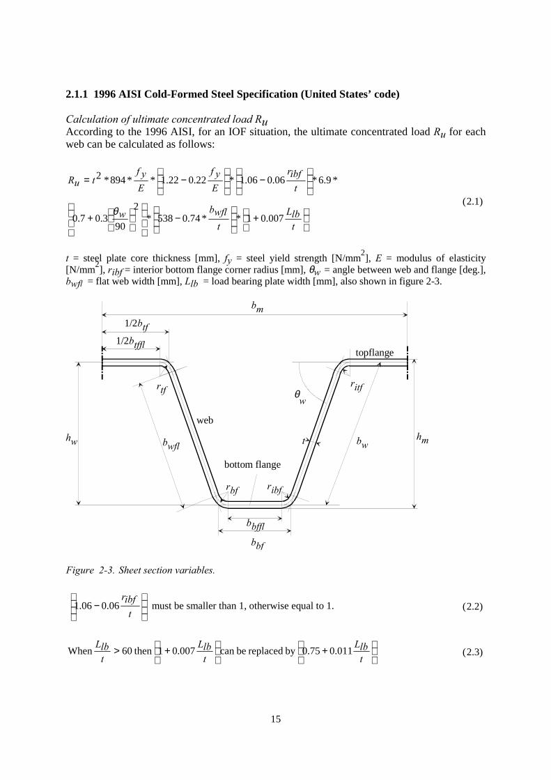
2.1.1 1996 AISI Cold-Formed Steel Specification (United States’ code)
Calculation of ultimate concentrated load RuAccording to the 1996 AISI, for an IOF situation, the ultimate concentrated load Ru for eachweb can be calculated as follows:
+
−
+
−
−=
tlbL
twflbw
tibfr
Eyf
Eyf
tuR
007.01**74.0538*2
903.07.0
*9.6*06.006.1*22.022.1**894*2
θ(2.1)
t = steel plate core thickness [mm], fy = steel yield strength [N/mm2], E = modulus of elasticity[N/mm2], ribf = interior bottom flange corner radius [mm], θw = angle between web and flange [deg.],bwfl = flat web width [mm], Llb = load bearing plate width [mm], also shown in figure 2-3.
bwfl bw
1/2btffl
bbf
bbffl
t
ritf
ribfrbf
rtf
hw hm
bm
topflange
bottom flange
web
1/2btf
θw
Figure 2-3. Sheet section variables.
−
tibfr
06.006.1 must be smaller than 1, otherwise equal to 1. (2.2)
+
+>
tlbL
tlbL
tlbL
011.075.0by replaced be can 007.01 then60 When (2.3)
16
For hat sections, the following conditions apply:
6/ ≤tibfr (2.4)
For sheet sections, the following conditions apply:
7/ ≤tibfr (2.5)
210/ ≤tlbL (2.6)
5.3/ ≤wflblbL (2.7)
It is not permitted to use strength increase from cold work of forming. The normal yieldstrength should be used.
Calculation of ultimate bending moment MuThe 1996 AISI has two different procedures to predict the ultimate bending moment Mu. Nodistinction is made between hat sections and sheet sections or sheeting in either procedure.
The first procedure predicts the ultimate bending moment if one of the outer fibres of thesheeting yields, be it a compressed or tensioned fibre. It is permitted to use strength increasefrom cold work of forming.
For shear lag effects, if the span length is smaller than 30 times half the distance between thewebs, the widths of flanges (whether in compression or in tension) should be reduced. TheAISI has a table for this.
For the compressed parts of the sheeting (parts of the web and the compressed bottom flange)effective widths are calculated. These effective widths are calculated as follows:
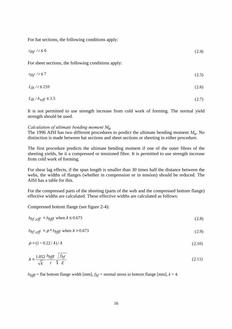
Compressed bottom flange (see figure 2-4):
673.0 when; ≤= λbfflbeffbfb (2.8)
673.0 when*; >= λρ bfflbeffbfb (2.9)
λλρ /)/22.01( −= (2.10)
Ebff
tbfflb
k052.1=λ (2.11)
bbffl = flat bottom flange width [mm], fbf = normal stress in bottom flange [mm], k = 4.
17
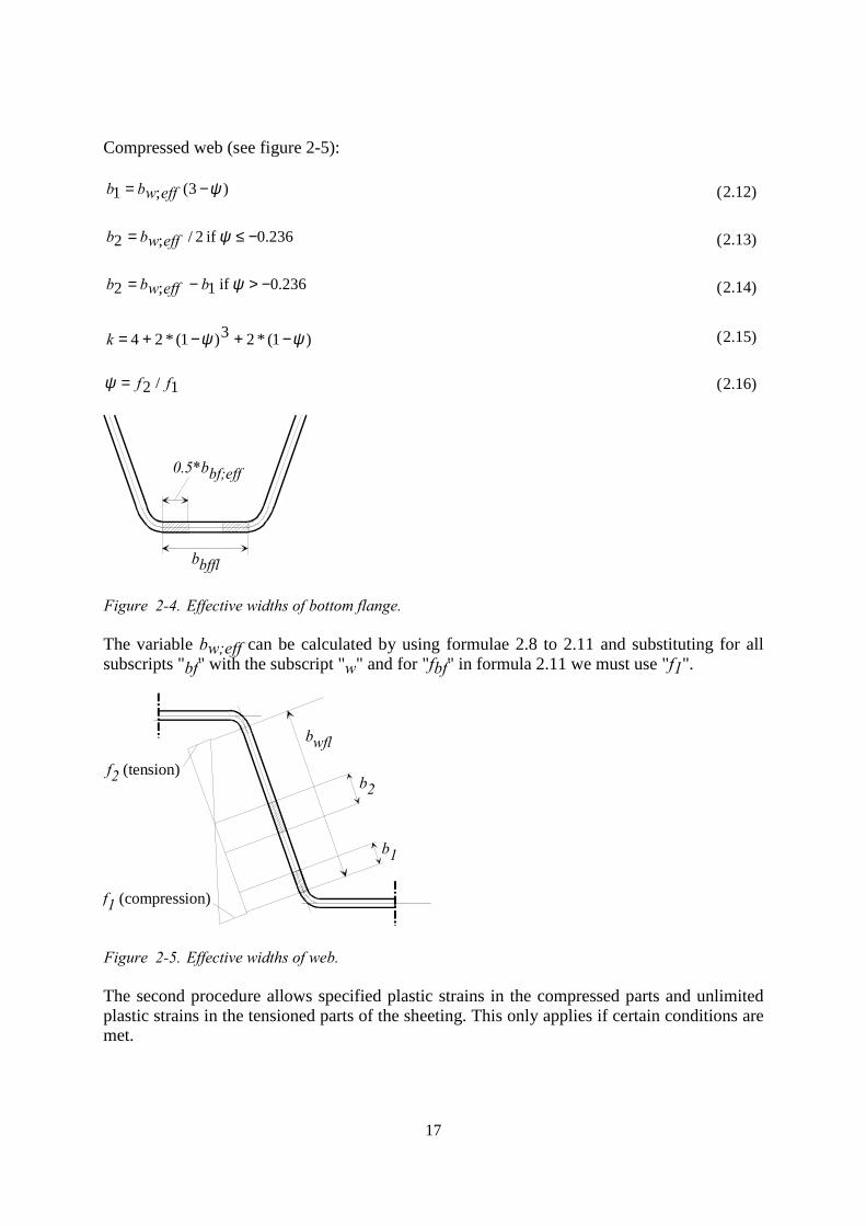
Compressed web (see figure 2-5):
)3(;1 ψ−= effwbb (2.12)
236.0 if 2/;2 −≤= ψeffwbb (2.13)
236.0 if 1;2 −>−= ψbeffwbb (2.14)
)1(*23)1(*24 ψψ −+−+=k (2.15)
1/2 ff=ψ (2.16)
bbffl
0.5*bbf;eff
Figure 2-4. Effective widths of bottom flange.
The variable bw;eff can be calculated by using formulae 2.8 to 2.11 and substituting for allsubscripts "bf" with the subscript "w" and for "fbf" in formula 2.11 we must use "f1".
bwfl
f1 (compression)
f2 (tension)
b1
b2
Figure 2-5. Effective widths of web.
The second procedure allows specified plastic strains in the compressed parts and unlimitedplastic strains in the tensioned parts of the sheeting. This only applies if certain conditions aremet.
18
Some of these conditions (relevant for this thesis) are as follows:
• The flange under compression (the bottom flange) should be fully effective for the firstprocedure.
• The ratio of the depth of the compressed portion of the web to its thickness does notexceed λ1 (formula 2.20). This ensures that the web is fully effective.
• The angle between web and flange θw should be larger than 70 degrees.
• The predicted ultimate bending moment should not exceed 1.25 times the ultimatebending moment found for the first procedure.
The second procedure is completely based on a paper of Reck, Peköz, and Winter [Reck75a].It is not permitted to use strength increase from cold work of forming.
The allowable plastic strain is obtained by multiplying the yield strain (fy/E) in thecompressed parts by a factor Cy that is calculated as follows:
1for 3 λ/tbfflbyC ≤= (2.17)
2/1for 12
1/23 λλ
λλλ
≤≤
−
−−= tbfflb
tbfflbyC (2.18)
2/for 1 λ≥= tbfflbyC (2.19)
Eyf /11.1
1 =λ (2.20)
Eyf /28.1
2 =λ (2.21)
Calculation of ultimate interaction load FuUsing the "Load Resistance and Factor Design (LRFD)" method, which is also used by theother two design codes, failure of sheeting is predicted as follows:
32.182.0 =+uM
M
uRuF
(2.22)
with:
4
)( lbLspanLuFM
−= (2.23)
19
2.1.2 S136-94 Cold Formed Steel Structural Members (Canadian code)
Calculation of ultimate concentrated load RuThe Canadian code [Cana95a] predicts the ultimate concentrated load as follows. Nodistinction is made between hat sections and sheeting, but for hat sections spreading of thewebs should be prevented.
( )
−
+
−=
twflb
tlbL
tibfr
wyftuR 04.01*065.01*12.01sin2*21 θ (2.24)
The above formula is valid for the following conditions:
10≤t
ibfr(2.25)
200≤tlbL
(2.26)
200≤t
wflb(2.27)
2≤wflblbL
(2.28)
It is not permitted to use strength increase from cold work of forming. The normal yieldstrength should be used.
Calculation of ultimate bending moment MuIn the Canadian code, the calculation of the ultimate bending moment Mu is exactly equal tothe United States’ code, except for the following items.
• Some formulae are written in a different format, such as the determination of effectivewidths. Due to different rounding of constants, these format differences are important.
• For the second procedure, an additional condition should apply:
yfE
twflb
73.3≤ (2.29)
20
Calculation of ultimate interaction load FuFor interaction of concentrated load and bending moment, the Canadian code demands thefollowing:
3.1=+uM
M
uRuF
(2.30)
with:
4
)( lbLspanLuFM
−= (2.31)
2.1.3 ENV 1993-1-3 Eurocode3 - Part 1-3 (European code)
Calculation of ultimate concentrated load RuThe European code predicts the ultimate concentrated load Ru for each web by the followingformula:
( ) ( ) ( )
++−= 290/4.2*/02.05.0*/1.01*2
wtlbLtibfrEyftuR θα (2.32)
The variable α depends on whether sheeting or sheet sections (0.075) or hat sections (0.057)are used. The formula is valid for the following conditions:
10≤t
ibfr(2.33)
9045 ≤≤ wθ (2.34)
200≤t
wflb(2.35)
It is not permitted to use strength increase from cold work of forming. The normal yieldstrength should be used.
Calculation of ultimate bending moment MuIn the European code, the calculation of the ultimate bending moment Mu is exactly equal tothe first procedure of the United States’ code, except for the following items.
• The effects of shear lag are presented in a more complex way. If the length between pointsof zero moment is less than 20 times half the distance between the webs, the widths offlanges (different for compression and tension) should be reduced. This reduction dependson the loading situation: an internal support of a continuous beam (sheeting in practice) ora span moment in a simple beam with central point load (three-point bending test).

21
• In the calculations for effective widths, not the flat widths bbffl and bwfl are used, but thedistances between the midpoints of corners.
• It is permitted to use strength increase from cold work of forming for fully effectiveflanges.
• Some formulae are written in a different format, e.g. the determination of effective widthsfor the web. Due to different rounding of constants, these format differences areimportant.
The conditions for allowable plastic strains in the compressed flange (second procedure) aredifferent:
• The angle between web and flange θw should be larger than 60 degrees.
• There is no such condition as in the United States’ code that the predicted ultimatebending moment should not exceed 1.25 times the ultimate bending moment found for thefirst procedure.
Calculation of ultimate interaction load FuFor interaction of concentrated load and bending moment, the European code requires thefollowing:
25.1=+uM
M
uRuF
(2.36)
with:
4
)( lbLspanLuFM
−= (2.37)
2.1.4 Differences for the three design codes
The three presented design codes have more similarities than differences. However, thedifferences are especially important. All three design codes have completely differentprocedures for finding Ru. Furthermore, the interaction ultimate load Fu is found usingdifferent values in the interaction formula for all three codes. Other differences concern thecalculation of ultimate bending moment Mu and are presented here.
Differences between Eurocode3 and the AISI:
1. The procedure taking shear lag into account is different for Eurocode3 and the AISI.
2. For the AISI, the ultimate bending moment found by the second procedure should notexceed 1.25 times the ultimate bending moment found via the first procedure. Eurocode 3does not have such a restriction.
22
3. The effective widths in Eurocode3 are based on a slightly larger width than the 1986 AISI.
4. The calculation of effective widths for the compressed part of the web is different forEurocode3 and the AISI.
5. Compared to Eurocode3, AISI has an additional constraint (regarding shear forces) toallow calculation of the bending moment via the second procedure.
Differences between the Canadian code and the AISI:
1. The constraints to allow calculation of the bending moment via the second procedure aredifferent for the Canadian code and the AISI.
2. The calculation of effective widths for the compressed part of the web is different for theCanadian code and the AISI.
2.1.5 Comparison of design codes
In chapter 5, section 5.2, experiments are selected from experiments presented in section2.2.3. These selected experiments are used in this section to compare the three design codespresented. The selected experiments are assumed to be suitable for making a comparison ofthe three design codes. Section 2.2.3 and chapter 5, section 5.2 will give a further explanationof the selected experiments.
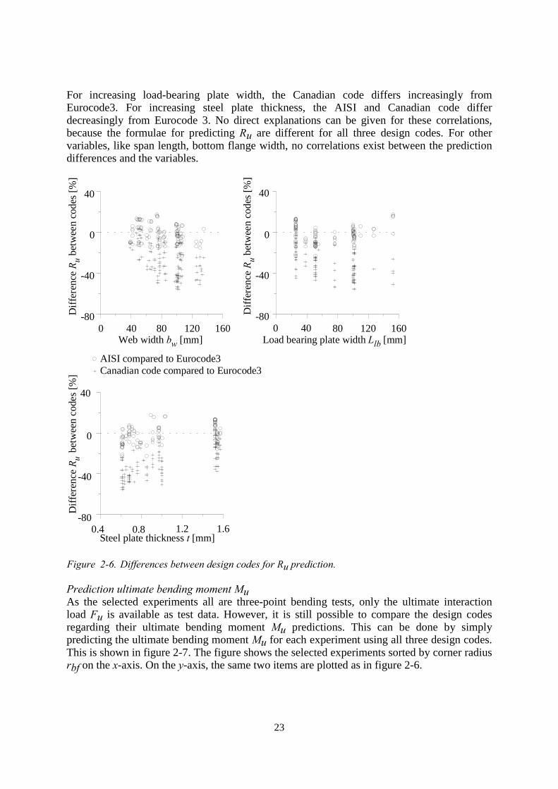
Prediction of ultimate concentrated load RuBecause the selected experiments all are three-point bending tests, only the ultimateinteraction load Fu is available as test data. However, it is still possible to compare the designcodes concerning their prediction of ultimate concentrated load Ru. This can be done bysimply predicting the ultimate concentrated load Ru for each experiment using all three designcodes. This is shown in figure 2-6. The first diagram in figure 2-6 shows the selectedexperiments sorted by web width bw on the x-axis. On the y-axis, two items are plotted. Forthe experiments indicated with a small circle, the difference of the AISI prediction to theEurocode3 prediction is plotted as follows for every experiment: ((AISI value - Eurocode3value) / Eurocode3 value) * 100%. For the experiments indicated with a small cross, thedifference of the Canadian code prediction to the Eurocode3 prediction is plotted for everyexperiment. The next two diagrams in figure 2-6 show the same results, however, now sortedby load-bearing plate width and steel plate thickness.
Figure 2-6 shows that AISI code predictions can differ between +18 and -22 % compared toEurocode3 predictions. Canadian code predictions can differ between +3 and -58 % comparedto Eurocode3 predictions.
For increasing web width, the Canadian code differs increasingly from Eurocode3. This maybe because Eurocode3 does not include the influence of the web width. However, the AISIdoes include the influence of the web width, but differences between the AISI and Eurocode3are not correlated to the web width.
23
For increasing load-bearing plate width, the Canadian code differs increasingly fromEurocode3. For increasing steel plate thickness, the AISI and Canadian code differdecreasingly from Eurocode 3. No direct explanations can be given for these correlations,because the formulae for predicting Ru are different for all three design codes. For othervariables, like span length, bottom flange width, no correlations exist between the predictiondifferences and the variables.
0 40 80 120 160Web width bw [mm]
-80
-40
0
40
Diff
eren
ce R
u be
twee
n co
des [
%]
AISI compared to Eurocode3Canadian code compared to Eurocode3
0 40 80 120 160Load bearing plate width Llb [mm]
-80
-40
0
40
Diff
eren
ce R
u bet
wee
n co
des [
%]
0.4 0.8 1.2 1.6Steel plate thickness t [mm]
-80
-40
0
40
Diff
eren
ce R
u be
twee
n co
des [
%]
Figure 2-6. Differences between design codes for Ru prediction.
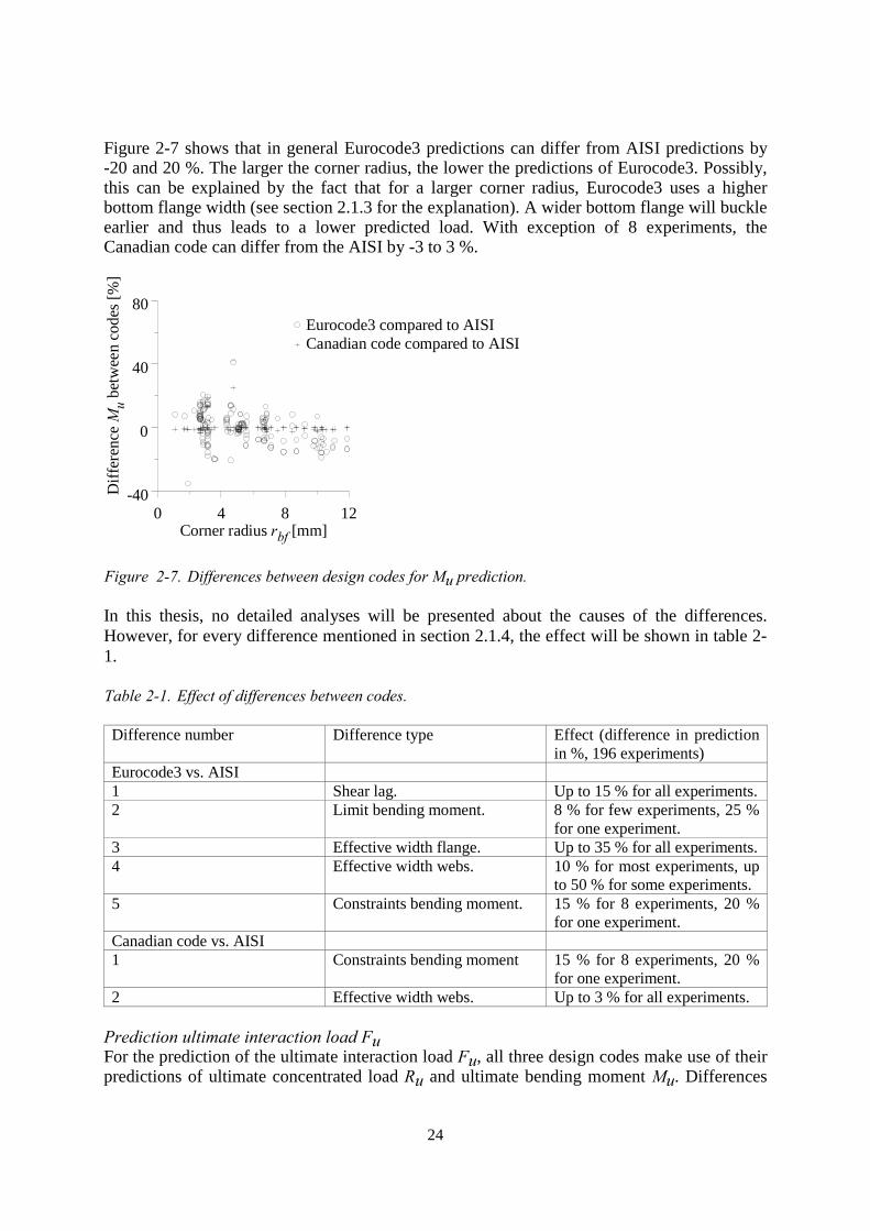
Prediction ultimate bending moment MuAs the selected experiments all are three-point bending tests, only the ultimate interactionload Fu is available as test data. However, it is still possible to compare the design codesregarding their ultimate bending moment Mu predictions. This can be done by simplypredicting the ultimate bending moment Mu for each experiment using all three design codes.This is shown in figure 2-7. The figure shows the selected experiments sorted by corner radiusrbf on the x-axis. On the y-axis, the same two items are plotted as in figure 2-6.
24
Figure 2-7 shows that in general Eurocode3 predictions can differ from AISI predictions by-20 and 20 %. The larger the corner radius, the lower the predictions of Eurocode3. Possibly,this can be explained by the fact that for a larger corner radius, Eurocode3 uses a higherbottom flange width (see section 2.1.3 for the explanation). A wider bottom flange will buckleearlier and thus leads to a lower predicted load. With exception of 8 experiments, theCanadian code can differ from the AISI by -3 to 3 %.
Corner radius rbf [mm]0 4 8 12
-40
0
40
80
Diff
eren
ce M
u be
twee
n co
des [
%]
Eurocode3 compared to AISICanadian code compared to AISI
Figure 2-7. Differences between design codes for Mu prediction.
In this thesis, no detailed analyses will be presented about the causes of the differences.However, for every difference mentioned in section 2.1.4, the effect will be shown in table 2-1.
Table 2-1. Effect of differences between codes.
Difference number Difference type Effect (difference in predictionin %, 196 experiments)
Eurocode3 vs. AISI1 Shear lag. Up to 15 % for all experiments.2 Limit bending moment. 8 % for few experiments, 25 %
for one experiment.3 Effective width flange. Up to 35 % for all experiments.4 Effective width webs. 10 % for most experiments, up
to 50 % for some experiments.5 Constraints bending moment. 15 % for 8 experiments, 20 %
for one experiment.Canadian code vs. AISI1 Constraints bending moment 15 % for 8 experiments, 20 %
for one experiment.2 Effective width webs. Up to 3 % for all experiments.
Prediction ultimate interaction load FuFor the prediction of the ultimate interaction load Fu, all three design codes make use of theirpredictions of ultimate concentrated load Ru and ultimate bending moment Mu. Differences
25
between codes for the prediction of Ru and Mu thus will also cause differences for Fu.Besides this, there are differences between the codes for the prediction of Fu itself: there aredifferent numerical values for the interaction formulae (for example formulae 2.30 and 2.36).
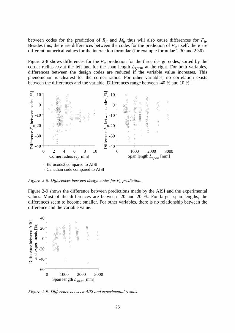
Figure 2-8 shows differences for the Fu prediction for the three design codes, sorted by thecorner radius rbf at the left and for the span length Lspan at the right. For both variables,differences between the design codes are reduced if the variable value increases. Thisphenomenon is clearest for the corner radius. For other variables, no correlation existsbetween the differences and the variable. Differences range between -40 % and 10 %.
Corner radius rbf [mm]0 2 4 6 8 10
-40
-30
-20
-10
0
10
Diff
eren
ce F
u bet
wee
n co
des [
%]
0 1000 2000 3000Span length Lspan [mm]
-40
-30
-20
-10
0
10
Diff
eren
ce F
u bet
wee
n co
des [
%]
Eurocode3 compared to AISICanadian code compared to AISI
Figure 2-8. Differences between design codes for Fu prediction.
Figure 2-9 shows the difference between predictions made by the AISI and the experimentalvalues. Most of the differences are between -20 and 20 %. For larger span lengths, thedifferences seem to become smaller. For other variables, there is no relationship between thedifference and the variable value.
0 1000 2000 3000Span length Lspan [mm]
-60
-40
-20
0
20
40
Diff
eren
ce b
etw
een
AIS
I a
nd e
xper
imen
ts [%
]
Figure 2-9. Difference between AISI and experimental results.

26
2.1.6 Conclusions
The three current design codes investigated (AISI, the Canadian code, and Eurocode3) allhave different formulae for predicting the ultimate concentrated load Ru. However, all threedesign codes developed these formulae by curve fitting experimental results. For the ultimateconcentrated load Ru, AISI predictions can differ between +18 and -22 % from Eurocode3predictions. Canadian code predictions can differ between +3 and -58 % from Eurocode3predictions.
The three design codes use the same concept to predict the ultimate concentrated load Mu.However, due to small differences in formulae and restrictions, Eurocode3 predictions candiffer from AISI predictions by between -20 and 20 %. With exception of 8 experiments, theCanadian code can differ from the AISI by -3 to 3 %.
The three design codes use the same concept for predicting the ultimate interaction load Fu.However, due to different numerical values in the formulae, there are differences between -40% and 10 %. Compared to experimental ultimate loads, the AISI predictions are between -20and 20 %.
27
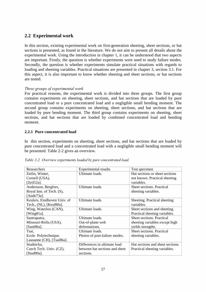
2.2 Experimental work
In this section, existing experimental work on first-generation sheeting, sheet sections, or hatsections is presented, as found in the literature. We do not aim to present all details about theexperimental work. Using the introduction in chapter 1, it can be understood that two aspectsare important. Firstly, the question is whether experiments were used to study failure modes.Secondly, the question is whether experiments simulate practical situations with regards toloading and sheeting variables. Practical situations are presented in chapter 3, section 3.1. Forthis aspect, it is also important to know whether sheeting and sheet sections, or hat sectionsare tested.
Three groups of experimental workFor practical reasons, the experimental work is divided into three groups. The first groupcontains experiments on sheeting, sheet sections, and hat sections that are loaded by pureconcentrated load or a pure concentrated load and a negligible small bending moment. Thesecond group contains experiments on sheeting, sheet sections, and hat sections that areloaded by pure bending moment. The third group contains experiments on sheeting, sheetsections, and hat sections that are loaded by combined concentrated load and bendingmoment.
2.2.1 Pure concentrated load
In this section, experiments on sheeting, sheet sections, and hat sections that are loaded bypure concentrated load and a concentrated load with a negligible small bending moment willbe presented. Table 2-2 gives an overview.
Table 2-2. Overview experiments loaded by pure concentrated load.
Researchers Experimental results Test specimenZetlin, Winter,Cornell (USA),[Zetl52a].
Ultimate loads. Hat sections or sheet sectionsnot known. Practical sheetingvariables.
Andersson, Bergfors,Royal Inst. of Tech. (S),[Ande73a].
Ultimate loads. Sheet sections. Practicalsheeting variables.
Keulers, Eindhoven Univ. ofTech., (NL), [Keul80a].
Ultimate loads. Sheeting. Practical sheetingvariables.
Wing, Waterloo (CAN),[Wing81a].
Ultimate loads. Sheet sections and sheeting.Practical sheeting variables.
Santraputra,Missouri-Rolla (USA),[Sant86a].
Ultimate loads.Out-of-plane webdeformations.
Sheet sections. Practicalsheeting variables except highyields strengths.
Tsai,Ecole Polytechnique,Lausanne (CH), [Tsai86a].
Ultimate loads.Photos of post-failure modes.
Sheet sections. Practicalsheeting variables.
Studnicka,Czech Tech. Univ. (CZ),[Stud90a].
Differences in ultimate loadbetween hat sections and sheetsections.
Hat sections and sheet sections.Practical sheeting variables.
28
Only a few sets of experiments provide some insight into the failure behaviour by presentingphotos of post-failure modes of sheeting. However, these photos are not detailed enough tostudy post-failure modes in depth. None of these experiments simulates the practical loadingsituation because only concentrated load (or concentrated load and a negligible small bendingmoment) is applied.
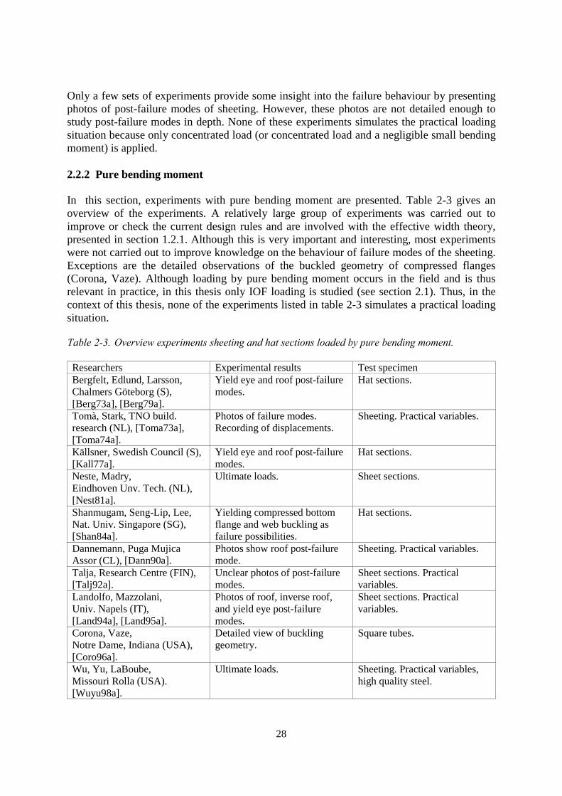
2.2.2 Pure bending moment
In this section, experiments with pure bending moment are presented. Table 2-3 gives anoverview of the experiments. A relatively large group of experiments was carried out toimprove or check the current design rules and are involved with the effective width theory,presented in section 1.2.1. Although this is very important and interesting, most experimentswere not carried out to improve knowledge on the behaviour of failure modes of the sheeting.Exceptions are the detailed observations of the buckled geometry of compressed flanges(Corona, Vaze). Although loading by pure bending moment occurs in the field and is thusrelevant in practice, in this thesis only IOF loading is studied (see section 2.1). Thus, in thecontext of this thesis, none of the experiments listed in table 2-3 simulates a practical loadingsituation.
Table 2-3. Overview experiments sheeting and hat sections loaded by pure bending moment.
Researchers Experimental results Test specimenBergfelt, Edlund, Larsson,Chalmers Göteborg (S),[Berg73a], [Berg79a].
Yield eye and roof post-failuremodes.
Hat sections.
Tomà, Stark, TNO build.research (NL), [Toma73a],[Toma74a].
Photos of failure modes.Recording of displacements.
Sheeting. Practical variables.
Källsner, Swedish Council (S),[Kall77a].
Yield eye and roof post-failuremodes.
Hat sections.
Neste, Madry,Eindhoven Unv. Tech. (NL),[Nest81a].
Ultimate loads. Sheet sections.
Shanmugam, Seng-Lip, Lee,Nat. Univ. Singapore (SG),[Shan84a].
Yielding compressed bottomflange and web buckling asfailure possibilities.
Hat sections.
Dannemann, Puga MujicaAssor (CL), [Dann90a].
Photos show roof post-failuremode.
Sheeting. Practical variables.
Talja, Research Centre (FIN),[Talj92a].
Unclear photos of post-failuremodes.
Sheet sections. Practicalvariables.
Landolfo, Mazzolani,Univ. Napels (IT),[Land94a], [Land95a].
Photos of roof, inverse roof,and yield eye post-failuremodes.
Sheet sections. Practicalvariables.
Corona, Vaze,Notre Dame, Indiana (USA),[Coro96a].
Detailed view of bucklinggeometry.
Square tubes.
Wu, Yu, LaBoube,Missouri Rolla (USA).[Wuyu98a].
Ultimate loads. Sheeting. Practical variables,high quality steel.
29
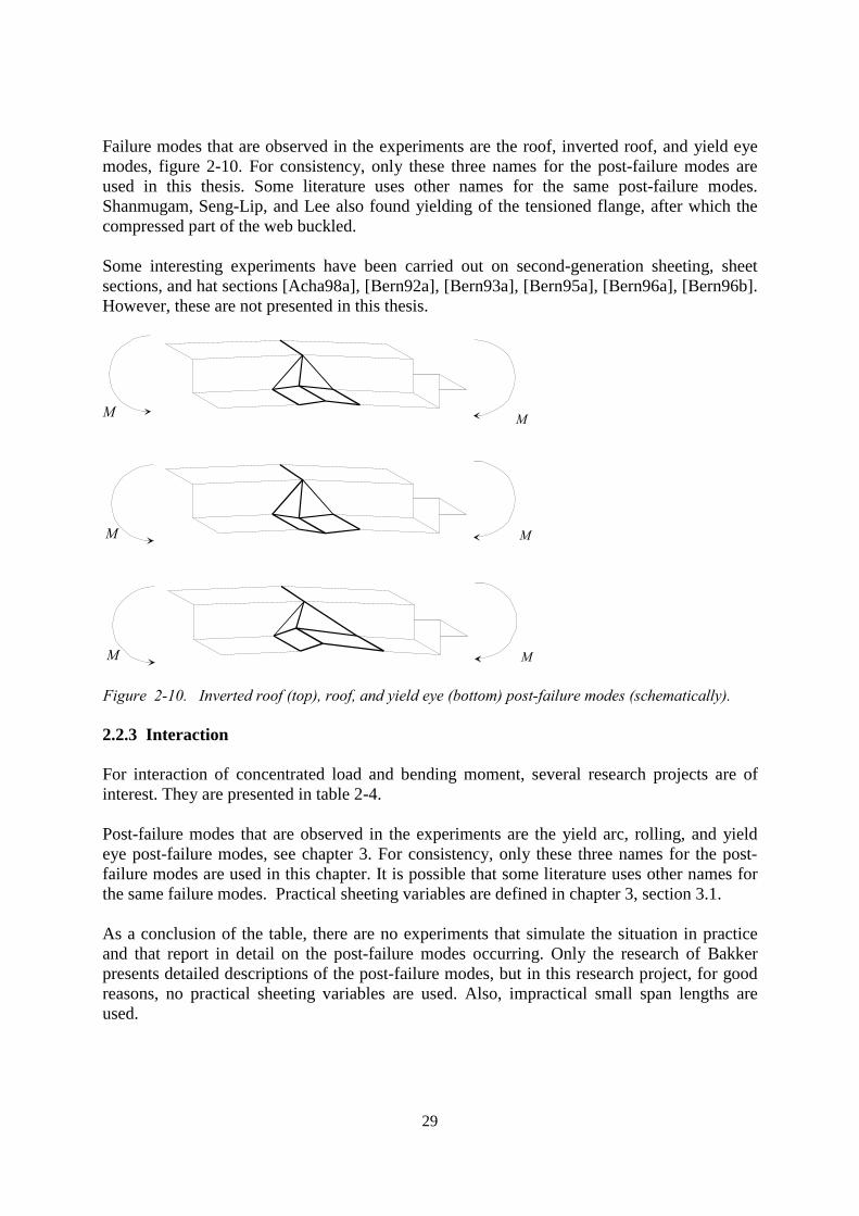
Failure modes that are observed in the experiments are the roof, inverted roof, and yield eyemodes, figure 2-10. For consistency, only these three names for the post-failure modes areused in this thesis. Some literature uses other names for the same post-failure modes.Shanmugam, Seng-Lip, and Lee also found yielding of the tensioned flange, after which thecompressed part of the web buckled.
Some interesting experiments have been carried out on second-generation sheeting, sheetsections, and hat sections [Acha98a], [Bern92a], [Bern93a], [Bern95a], [Bern96a], [Bern96b].However, these are not presented in this thesis.
M M
M M
M M
Figure 2-10. Inverted roof (top), roof, and yield eye (bottom) post-failure modes (schematically).
2.2.3 Interaction
For interaction of concentrated load and bending moment, several research projects are ofinterest. They are presented in table 2-4.
Post-failure modes that are observed in the experiments are the yield arc, rolling, and yieldeye post-failure modes, see chapter 3. For consistency, only these three names for the post-failure modes are used in this chapter. It is possible that some literature uses other names forthe same failure modes. Practical sheeting variables are defined in chapter 3, section 3.1.
As a conclusion of the table, there are no experiments that simulate the situation in practiceand that report in detail on the post-failure modes occurring. Only the research of Bakkerpresents detailed descriptions of the post-failure modes, but in this research project, for goodreasons, no practical sheeting variables are used. Also, impractical small span lengths areused.

30
Table 2-4. Overview experiments sheeting, sheet sections, and hat sections under interaction load.
Researchers Test results Practical situations simulatedZetlin, Winter, Cornell (USA),[Zetl52a].
Ultimate loads. Sheet or hat sections notknown. Practical variables
Tomà, Stark, TNO build.research (NL), [Toma73a],[Toma74a].
Photos of failure modes.Recording of displacements.
Sheeting. Practical variables.Three point bending tests andtwo span tests.
Keulers, Eindhoven (NL),[Keul80a], [Keul81a].
Ultimate loads. Sheet sections and sheeting.Practical variables.
Wing, Waterloo (CAN),[Wing81a].
Ultimate loads. Sheet sections and sheeting.Practical variables.
Santraputra, Missouri-Rolla(USA), [Sant86a].
Out-of-plane web deformationshave been recorded.
Sheet sections. High yieldstrengths.
Tsai, Ecole Tech. Lausanne(CH), [Tsai86a].
Photos of failure modes. Sheet sections. Practicalsheeting variables.
Bakker, Eindhoven Unv. Tech.(NL), [Bakk92a].
Detailed description: yield arcand rolling failure modes.
Sheet sections. No practicalsheeting variables.
31
2.3 Finite element models
Although finite element models have been available since the beginning of the sixties, finiteelement models for sheeting still are sparse. Finite element models are useful for modellingsheeting for three reasons. Firstly, they can partly substitute expensive experiments forsystematic variation of variables. Secondly, they can be used to test all sorts of assumptionsand hypotheses about sheeting failure. Thirdly, they can simulate experiments that arepractically impossible but worthy of study. For example, it is possible to investigate howsheeting behaves for extremely long span lengths.
In chapter 4, it will be shown that the finite element modelling of the corner between web andflange is very important. Furthermore, chapter 3 will show that for a specific failure mode, ahalf finite element model is necessary, instead of a normally used quarter model. These twoaspects, the modelling of the corner and the model type, will be given special attention in thissection. Below, the finite element models are listed in chronological sequence.
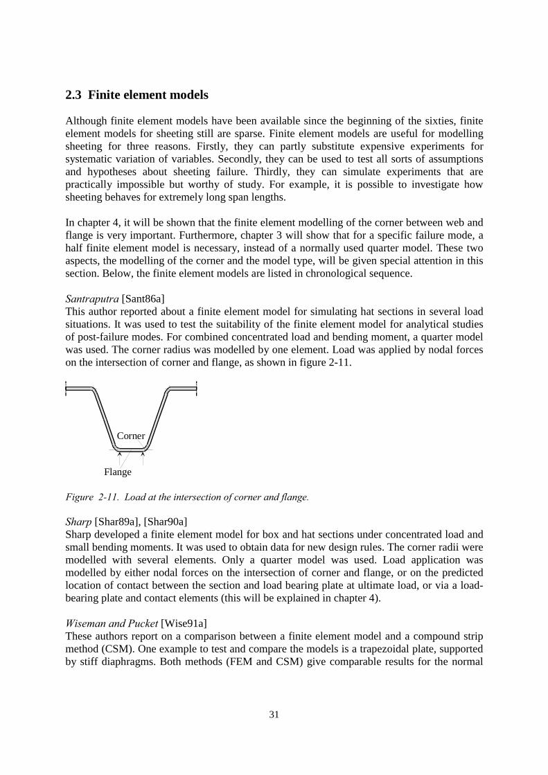
Santraputra [Sant86a]This author reported about a finite element model for simulating hat sections in several loadsituations. It was used to test the suitability of the finite element model for analytical studiesof post-failure modes. For combined concentrated load and bending moment, a quarter modelwas used. The corner radius was modelled by one element. Load was applied by nodal forceson the intersection of corner and flange, as shown in figure 2-11.
Corner
Flange
Figure 2-11. Load at the intersection of corner and flange.
Sharp [Shar89a], [Shar90a]Sharp developed a finite element model for box and hat sections under concentrated load andsmall bending moments. It was used to obtain data for new design rules. The corner radii weremodelled with several elements. Only a quarter model was used. Load application wasmodelled by either nodal forces on the intersection of corner and flange, or on the predictedlocation of contact between the section and load bearing plate at ultimate load, or via a load-bearing plate and contact elements (this will be explained in chapter 4).
Wiseman and Pucket [Wise91a]These authors report on a comparison between a finite element model and a compound stripmethod (CSM). One example to test and compare the models is a trapezoidal plate, supportedby stiff diaphragms. Both methods (FEM and CSM) give comparable results for the normal
32
stresses in the compression flange. Corner radii are not modelled. Load application involves auniformly distributed load. Only elastic behaviour is investigated.
Talja [Talj92a]The author presents a finite element model for pure bending and one model for combinedconcentrated load and bending tests for open sections. For the bending tests, long specimenswere given an imperfection; smaller specimens did not contain an imperfection. Very littledetailed information on the finite element model itself is given. For the combinedconcentrated load and bending tests, the corner radius was modelled with only one element.For hat sections studied, the corner radius was ignored. Load application involved nodalforces on the intersection of corner and flange, see figure 2-11.
Landolfo and Mazzolani [Land94a], [Land95a]These authors carried out a large experimental program on pure bending of hat sections. Theyalso modelled the experiments with a finite element model, but details on the model are notgiven. The aim of the finite element model is to create moment versus curvature diagrams andto compare them with the experiments. The best results are within 25 % of the experimentalvalues.
Vaessen [Vaes95a]The author developed a quarter finite element model to study the elastic behaviour of hatsections in three-point bending tests. Corner radii are accurately modelled with severalelements. Load is applied by nodal forces on the intersection of corner and flange. This modelis possibly inaccurate for large load-bearing plate widths.
Schafer and Peköz [Scha97a]For this research project sheeting with stiffeners was modelled with the finite element methodand loaded by pure bending moment. This was done to study the ultimate bending momentbehaviour. Corner radii are not modelled. A quarter model was used.
Davies and Jian [Davi97a]These authors present a finite element model for three commercial types of sheeting. This is aquarter model. The load of the intermediate support is modelled as nodal forces on theintersection of flange and web. Corner radii are not modelled. The model is used to show thatfor a specific area in the interaction diagram, extra strength is available.
Samanta and Mukhopadhyay [Sama99a]In order to make the analysis of trapezoidal sheeting less complicated, these authors suggestcarrying out an orthotropic analysis including bending rigidities. Finite element models ofsheeting and the proposed method are compared and it is proposed that the orthotropicanalysis including bending rigidities can be used as an alternative to the finite elementmethod. Corner radii are not modelled. Load application involves a uniformly distributedload. Only the elastic stresses in the sheeting are compared.
In chapter 4, the finite element model shows the need to model the corner radius with severalelements in cross-section direction (1), at least for the rolling post-failure mode. It also showsthe need to use a load bearing plate and contact elements to model the load application (2), at

33
least for the rolling post-failure mode. Finally, asymmetrical post-failure modes can occur(chapter 3). To cover these asymmetric post-failure modes, a whole or half finite elementmodel is needed. Table 2-5 gives an overview of the finite element models for these threeaspects. It shows that not one single finite element model follows all three requirements.
Table 2-5. Overview finite element models for sheeting and hat sections.
Author(s) Aim Corner modellingin cross-section
Load application Complete, half,or quarter model
Santraputra(1986).
Suitabilityelement models.
1 element. Nodal forces. Quarter.
Sharp (1990). Data for designrules.
Several elements. Nodal forces orload bearingplate.
Quarter.
Wiseman andPucket (1991).
Differences FEM/CSM.
Sharp (norounding ofcorner).
Uniformlydistributed load.
Complete.
Talja (1992). Behaviour thickwalled columns.
Max. 1 element. Nodal forces. Half.
Landolfo andMazzolani (1994,1995).
Moment rotationcurves.
Sharp (norounding ofcorner).
Nodal rotations. Not known.
Vaessen (1995). Elastic webstiffness.
Several elements. Nodal forces. Quarter.
Schafer andPeköz (1997).
Researchintermediatestiffeners.
Sharp (norounding ofcorner).
Nodal rotations. Quarter.
Davies and Jian(1997).
Basis for newmech. model.
Sharp (norounding ofcorner).
Nodal forces. Quarter.
Samanta andMukhopadhyay(1999).
Differences FEM/orthotropicmodels.
Sharp (norounding ofcorner).
Uniformlydistributed load.
Quarter.
34
2.4 Mechanical models
In the past, some efforts have been made to develop mechanical models for sheeting failurebehaviour. In all these cases, there are two possible reasons to develop these models: the needfor understandable design rules and the need for taking into account moment redistribution.Only the first reason will be a subject in this section. For moment redistribution, see[Bleu70a], [Unge73a], [Wang73a], [Yene85a], [Luur93a], [Thom96a], [Davi97a], [Soko97a]and [Soko98a].
Important aspectsThree important aspects are pertinent to mechanical models. Firstly, the model concept: themodel can be developed by means of yield line theory, elastic theory, etc. Secondly, thereason for developing the model. As already mentioned, most models are developed to obtainunderstandable design rules or to include moment redistribution. Finally, the load situationsfor which the model is developed: for concentrated load only, for bending moment only, orfor interaction. These three aspects will be used to discuss the mechanical models. In thesection below, mechanical models are presented in chronological order.
RSD [Rsdm74a]This was the first mechanical model for sheeting failure used in a Dutch design code. Itprovides insight into the failure behaviour by predicting the buckling load of the web due toseveral loads: the concentrated load of the support, a bending moment due to the off-centreapplication of the concentrated load, and the bending moment in the sheeting.
Bähr [Bahr78a]For sheeting under pure concentrated load at an end support, Bähr developed an analyticalmodel to predict the ultimate load. For this model, the elastic moment and force distributionsin the cross-section are calculated. Along the longitudinal direction, a parabolic distribution ofthese moments and forces is assumed. If the cross-section above the support yields, thesection is considered to have failed.
Reinsch [Rein83a]Reinsch developed a mechanical model for sheeting to be able to account for momentredistribution. However, his model can also be used to determine the failure load of sheeting.Using ITF tests, Reinsch derives an empirical formula to predict the ultimate concentratedload. By making the internal energy for ITF and IOF situations equal, the ultimate load can bederived for combined concentrated load and bending moment.
Tsai [Tsai86a]Tsai developed a mechanical model to find the ultimate load for sheeting. The concentratedload - deformation curve found by Reinsch is empirically modified for the bending moment.
Bakker [Bakk92a]Bakker carried out experiments on hat sections with a concentrated load only, or with aconcentrated load and a small bending moment. Two failure modes were observed: the rollingand the yield arc modes. These modes are briefly described in section 3.3.2 and figure 3-22. Ayield line model was developed for the rolling mode, see figure 2-12. Moving yield lines were
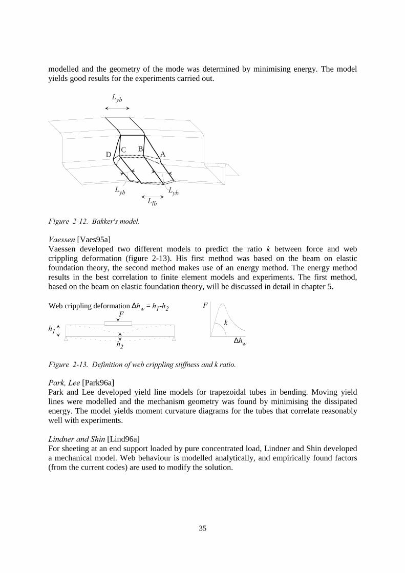
35
modelled and the geometry of the mode was determined by minimising energy. The modelyields good results for the experiments carried out.
ABCD
Llb
Lyb
Lyb Lyb
Figure 2-12. Bakker's model.
Vaessen [Vaes95a]Vaessen developed two different models to predict the ratio k between force and webcrippling deformation (figure 2-13). His first method was based on the beam on elasticfoundation theory, the second method makes use of an energy method. The energy methodresults in the best correlation to finite element models and experiments. The first method,based on the beam on elastic foundation theory, will be discussed in detail in chapter 5.
F
kh1
h2
Web crippling deformation ∆hw = h1-h2
∆hw
F
Figure 2-13. Definition of web crippling stiffness and k ratio.
Park, Lee [Park96a]Park and Lee developed yield line models for trapezoidal tubes in bending. Moving yieldlines were modelled and the mechanism geometry was found by minimising the dissipatedenergy. The model yields moment curvature diagrams for the tubes that correlate reasonablywell with experiments.
Lindner and Shin [Lind96a]For sheeting at an end support loaded by pure concentrated load, Lindner and Shin developeda mechanical model. Web behaviour is modelled analytically, and empirically found factors(from the current codes) are used to modify the solution.

36
Schafer and Peköz [Scha98a]Schafer and Peköz presented a model for the prediction of the ultimate bending moment ofcold-formed steel members. For existing tests, they calculated the buckling load using a finitestrip model. They discovered a relationship between the member slenderness and the strength.Therefore, they suggest to use a method to predict the ultimate load in which this relationshipis used at the member level. Traditional effective width methods work at the element level(only for webs or flange under compression).
Davies, Jian, Liu [Davi99a]These authors announce the development of a two-dimensional model for the hat sectioncross-section. This model will be checked by a two-dimensional finite element model. Infuture, the authors want to use the model for real three-dimensional sections.
Rhodes, Nash, and Macdonald [Rhod99a]For web crippling of thin-walled beams, finite element models and an energy model are usedto find the buckling load of the web. Then a Perry-Robertson approach was used to predict theultimate load of the webs. Only the Interior Two Flange (ITF) loading situation is observed.For this loading situation, the method yields satisfactory results.
OverviewTable 2-6 presents an overview of the mechanical models presented. The load situation oftenequals a concentrated load and a small impractical bending moment. One model wasdeveloped for pure bending, mainly to demonstrate the general approach of the yield linetheory. The model by Davies, Jian and Liu, which is not presented in literature yet, wasdeveloped for a practical range of concentrated load and bending moment.
DiscussionAs table 2-6 shows, four models exist or are in development for a practical load situation(concentrated load and bending moment). Two of them (Reinsch, Tsai) use empiricallyderived formulae. For a model in development (Davies, Jian, Liu), only the cross-sectionbehaviour of sheeting is modelled in this new model. The fourth model (RSD-model) predictssheeting failure by calculating the web buckling load. However, in chapter 4 it will be shownthat failure occurs mainly by yielding of the bottom corner.

37
Table 2-6. Mechanical models.
Authors Model concept Reason for developing Load situationRSD-Model,(1974).
Web buckling underseveral loads.
New design rule. Concentrated load andbending moment.
Bähr,(1987).
Elastic equilibrium. Improve currentempirical rule.
Concentrated loadonly.
Reinsch,(1983).
Empiricallydeterminedconcentrated load andenergy equilibrium.
Moment redistribution,but also suitable forprediction model.
Concentrated load andbending moment.
Tsai,(1986).
Empiricallydeterminedconcentrated load andcombined load.
New design rule. Concentrated load andbending moment.
Bakker,(1992).
Yield line. New design rule. Concentrated load andsmall (not practical)bending moment.
Vaessen,(1995).
Energy method. Finding elasticbehaviour for Bakkermodel.
Concentrated load andsmall (not practical)bending moment.
Park,Lee,(1996).
Yield line. Presenting generalapproach.
Pure bending.
Lindner,Shin,(1996).
Buckling of plate withsprings.
Improve currentempirical rule.
Concentrated load andsmall (not practical)bending moment.
Schafer and Peköz,(1998).
Relationship betweenslenderness andstrength.
More easy use ofdesign rules forcomplex cross-sections.
Pure bending.
Davies, Jian,Liu,(1999).
Not known, indevelopment.
New design rule. Concentrated load andsmall bendingmoment.
Rhodes, Nash,Macdonald,(1999).
Buckling load byenergy method.Ultimate load byPerry-Robertsonformulae.
Better design rules. Pure concentratedload.

38
2.5 Conclusions
To predict sheeting failure for the intermediate support, current design rules use the followingconcept. If only a concentrated load F acts on the sheeting, this load should not exceed theultimate concentrated load Ru. The same is valid for bending moment M and ultimate bendingmoment Mu. If a combination of F and M is present, the design rules limit the sum of F/Ruand M/Mu.
All three presented design codes are different concerning their prediction of the ultimateconcentrated load. The European code does not include the influence of the web width bwfl.
The effects of shear lag are calculated differently in the European code when compared withthe other two codes.
In chapter 4, we suggest that a finite element model should model the corner radius withseveral elements in cross-section direction (1), at least for the rolling post-failure mode. It isalso advisable to use a load bearing plate and contact elements to model the load application(2), at least for the rolling post-failure mode. Finally, as will be shown in chapter 3,asymmetrical post-failure modes can occur. To cover these asymmetric post-failure modes, awhole or half finite element model is needed. Existing finite element models do not follow allthree requirements.
Four mechanical models exist or are in development for a practical load situation(concentrated load and bending moment). Two of them (Reinsch and Tsai) partly useempirically derived formulae. For a model in development of Davies, Jian, and Liu, only thecross-section behaviour of sheeting is modelled at present. The fourth model (RSD-model)predicts sheeting failure by calculating the web buckling load. However, in chapter 4 it willbe shown that failure occurs mainly by yielding of the bottom corner.

39
3 Experiments
Chapter abstractThree point bending tests on sheet sections were carried out. Span length and cross-sectionvariables were chosen to simulate sheeting in practice. Three post-failure modes occur: therolling, yield arc and yield eye post-failure modes. Only the yield arc and yield eye post-failure modes are relevant.
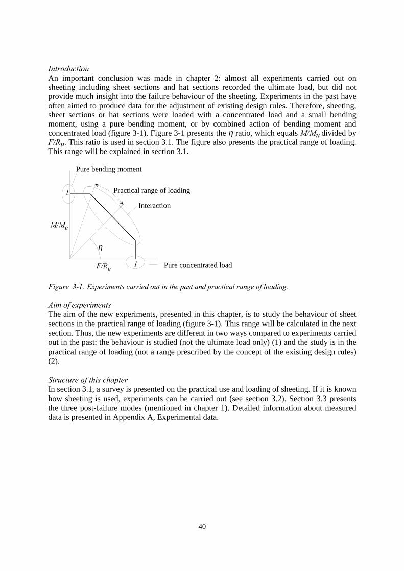
40
IntroductionAn important conclusion was made in chapter 2: almost all experiments carried out onsheeting including sheet sections and hat sections recorded the ultimate load, but did notprovide much insight into the failure behaviour of the sheeting. Experiments in the past haveoften aimed to produce data for the adjustment of existing design rules. Therefore, sheeting,sheet sections or hat sections were loaded with a concentrated load and a small bendingmoment, using a pure bending moment, or by combined action of bending moment andconcentrated load (figure 3-1). Figure 3-1 presents the η ratio, which equals M/Mu divided byF/Ru. This ratio is used in section 3.1. The figure also presents the practical range of loading.This range will be explained in section 3.1.
M/Mu
F/Ru1
1
Interaction
Pure concentrated load
Pure bending moment
η
Practical range of loading
Figure 3-1. Experiments carried out in the past and practical range of loading.
Aim of experimentsThe aim of the new experiments, presented in this chapter, is to study the behaviour of sheetsections in the practical range of loading (figure 3-1). This range will be calculated in the nextsection. Thus, the new experiments are different in two ways compared to experiments carriedout in the past: the behaviour is studied (not the ultimate load only) (1) and the study is in thepractical range of loading (not a range prescribed by the concept of the existing design rules)(2).
Structure of this chapterIn section 3.1, a survey is presented on the practical use and loading of sheeting. If it is knownhow sheeting is used, experiments can be carried out (see section 3.2). Section 3.3 presentsthe three post-failure modes (mentioned in chapter 1). Detailed information about measureddata is presented in Appendix A, Experimental data.
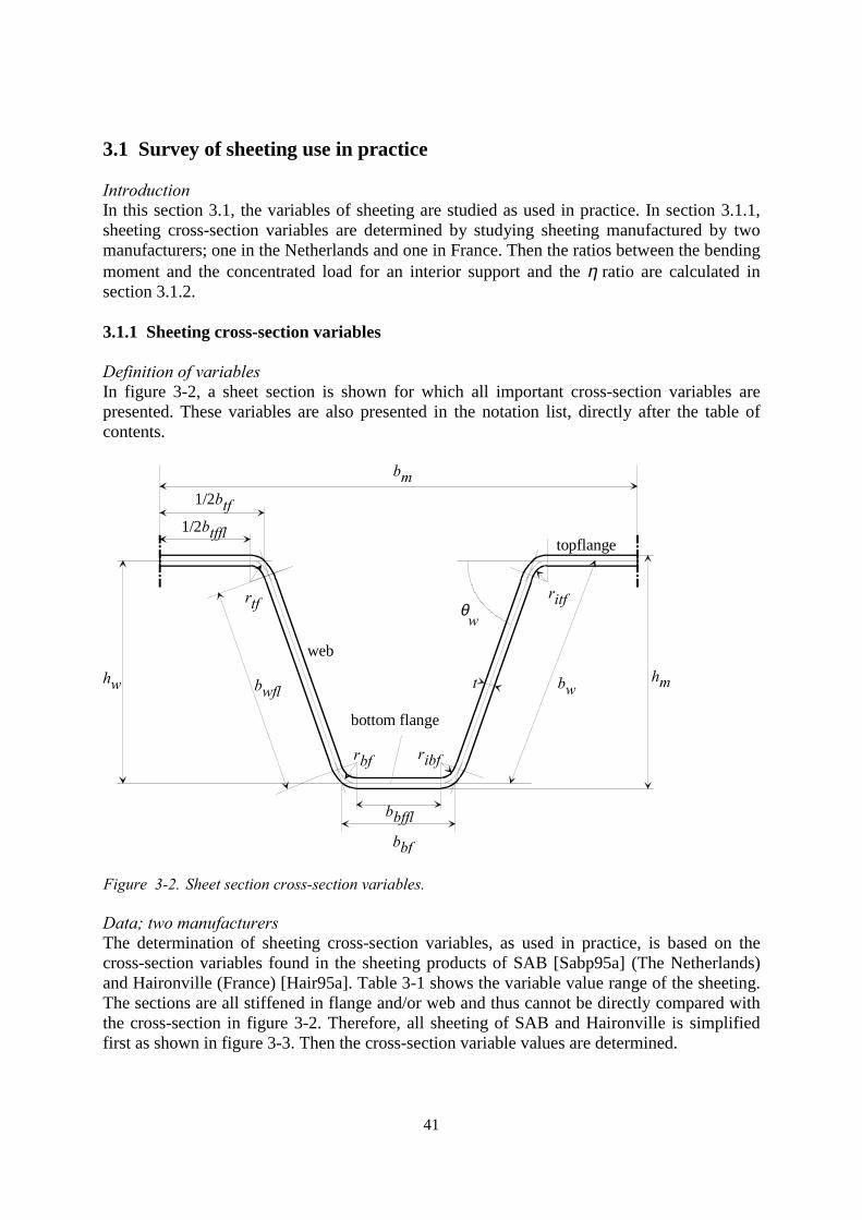
41
3.1 Survey of sheeting use in practice
IntroductionIn this section 3.1, the variables of sheeting are studied as used in practice. In section 3.1.1,sheeting cross-section variables are determined by studying sheeting manufactured by twomanufacturers; one in the Netherlands and one in France. Then the ratios between the bendingmoment and the concentrated load for an interior support and the η ratio are calculated insection 3.1.2.
3.1.1 Sheeting cross-section variables
Definition of variablesIn figure 3-2, a sheet section is shown for which all important cross-section variables arepresented. These variables are also presented in the notation list, directly after the table ofcontents.
bwfl bw
1/2btffl
bbf
bbffl
t
ritf
ribfrbf
rtf
hw hm
bm
topflange
bottom flange
web
1/2btf
θw
Figure 3-2. Sheet section cross-section variables.
Data; two manufacturersThe determination of sheeting cross-section variables, as used in practice, is based on thecross-section variables found in the sheeting products of SAB [Sabp95a] (The Netherlands)and Haironville (France) [Hair95a]. Table 3-1 shows the variable value range of the sheeting.The sections are all stiffened in flange and/or web and thus cannot be directly compared withthe cross-section in figure 3-2. Therefore, all sheeting of SAB and Haironville is simplifiedfirst as shown in figure 3-3. Then the cross-section variable values are determined.
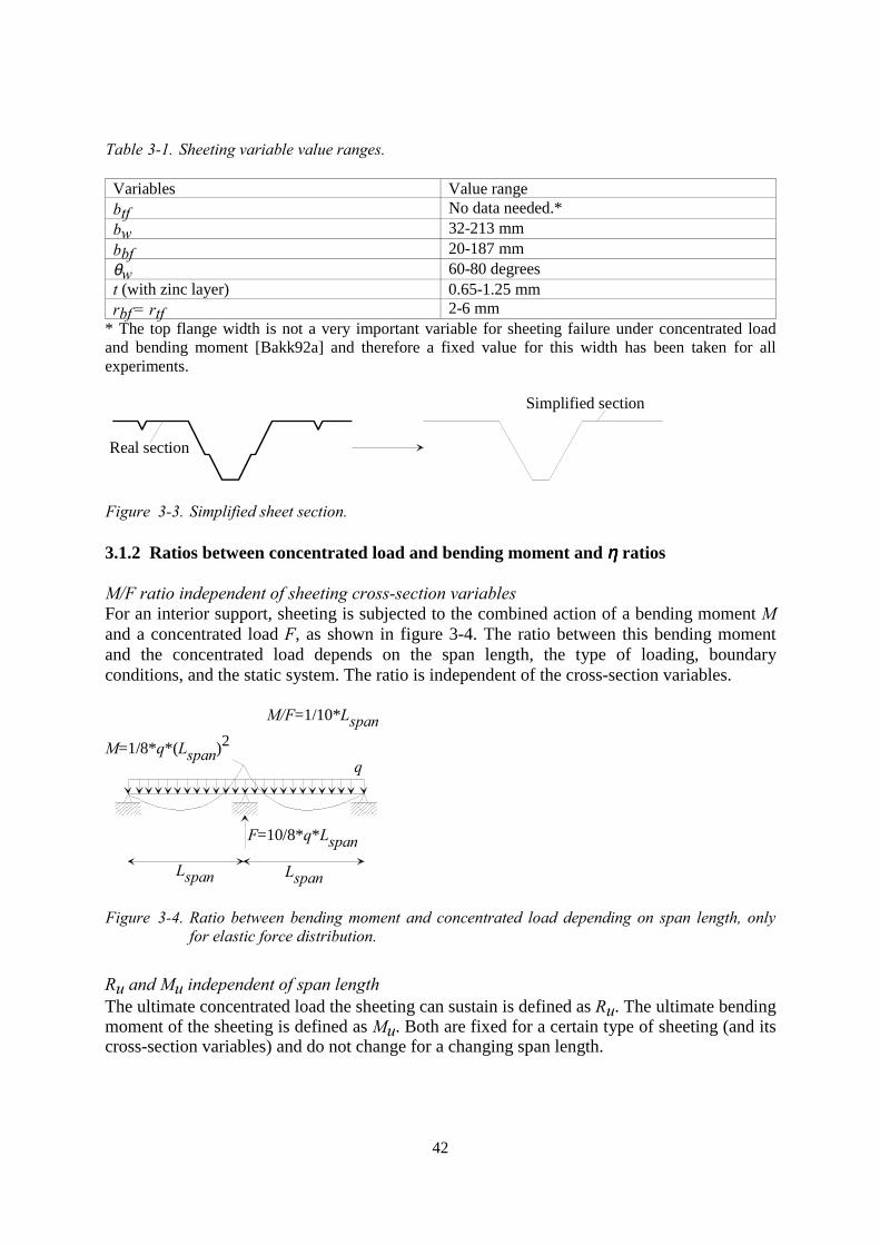
42
Table 3-1. Sheeting variable value ranges.
Variables Value rangebtf No data needed.*bw 32-213 mmbbf 20-187 mmθw 60-80 degreest (with zinc layer) 0.65-1.25 mmrbf = rtf 2-6 mm
* The top flange width is not a very important variable for sheeting failure under concentrated loadand bending moment [Bakk92a] and therefore a fixed value for this width has been taken for allexperiments.
Real section
Simplified section
Figure 3-3. Simplified sheet section.
3.1.2 Ratios between concentrated load and bending moment and ηηηη ratios
M/F ratio independent of sheeting cross-section variablesFor an interior support, sheeting is subjected to the combined action of a bending moment Mand a concentrated load F, as shown in figure 3-4. The ratio between this bending momentand the concentrated load depends on the span length, the type of loading, boundaryconditions, and the static system. The ratio is independent of the cross-section variables.
M=1/8*q*(Lspan)2
F=10/8*q*Lspan
q
Lspan
M/F=1/10*Lspan
Lspan
Figure 3-4. Ratio between bending moment and concentrated load depending on span length, onlyfor elastic force distribution.
Ru and Mu independent of span lengthThe ultimate concentrated load the sheeting can sustain is defined as Ru. The ultimate bendingmoment of the sheeting is defined as Mu. Both are fixed for a certain type of sheeting (and itscross-section variables) and do not change for a changing span length.
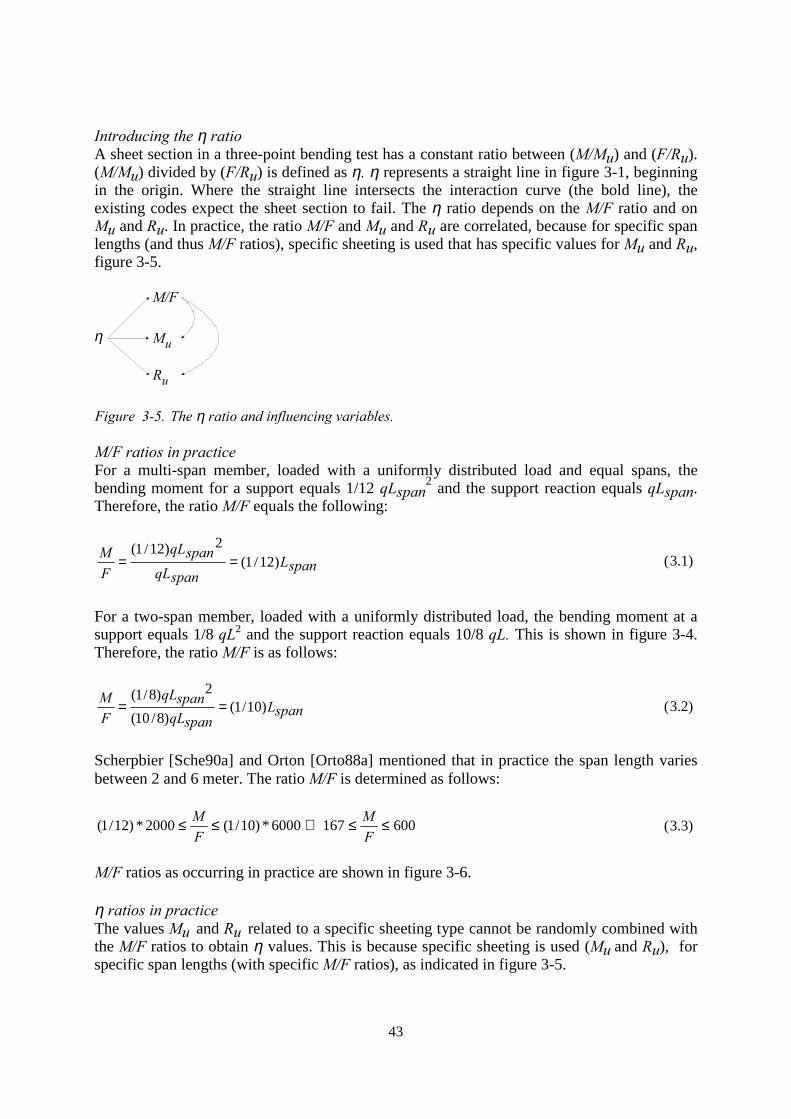
43
Introducing the η ratioA sheet section in a three-point bending test has a constant ratio between (M/Mu) and (F/Ru).(M/Mu) divided by (F/Ru) is defined as η. η represents a straight line in figure 3-1, beginningin the origin. Where the straight line intersects the interaction curve (the bold line), theexisting codes expect the sheet section to fail. The η ratio depends on the M/F ratio and onMu and Ru. In practice, the ratio M/F and Mu and Ru are correlated, because for specific spanlengths (and thus M/F ratios), specific sheeting is used that has specific values for Mu and Ru,figure 3-5.
η
M/F
Mu
Ru
Figure 3-5. The η ratio and influencing variables.
M/F ratios in practiceFor a multi-span member, loaded with a uniformly distributed load and equal spans, thebending moment for a support equals 1/12 qLspan
2 and the support reaction equals qLspan.Therefore, the ratio M/F equals the following:
spanLspanqL
spanqL
FM )12/1(
2)12/1(== (3.1)
For a two-span member, loaded with a uniformly distributed load, the bending moment at asupport equals 1/8 qL2 and the support reaction equals 10/8 qL. This is shown in figure 3-4.Therefore, the ratio M/F is as follows:
spanLspanqL
spanqLFM )10/1(
)8/10(
2)8/1(== (3.2)
Scherpbier [Sche90a] and Orton [Orto88a] mentioned that in practice the span length variesbetween 2 and 6 meter. The ratio M/F is determined as follows:
6001676000*)10/1(2000*)12/1( ≤≤⇔≤≤FM
FM (3.3)
M/F ratios as occurring in practice are shown in figure 3-6.
η ratios in practiceThe values Mu and Ru related to a specific sheeting type cannot be randomly combined withthe M/F ratios to obtain η values. This is because specific sheeting is used (Mu and Ru), forspecific span lengths (with specific M/F ratios), as indicated in figure 3-5.
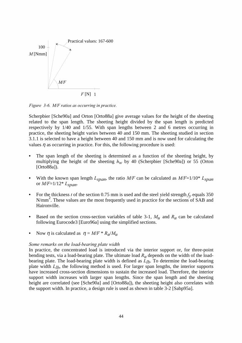
44
1
100M [Nmm]
F [N]
Practical values: 167-600
M/F
Figure 3-6. M/F ratios as occurring in practice.
Scherpbier [Sche90a] and Orton [Orto88a] give average values for the height of the sheetingrelated to the span length. The sheeting height divided by the span length is predictedrespectively by 1/40 and 1/55. With span lengths between 2 and 6 metres occurring inpractice, the sheeting height varies between 40 and 150 mm. The sheeting studied in section3.1.1 is selected to have a height between 40 and 150 mm and is now used for calculating thevalues η as occurring in practice. For this, the following procedure is used:
• The span length of the sheeting is determined as a function of the sheeting height, bymultiplying the height of the sheeting hw by 40 (Scherpbier [Sche90a]) or 55 (Orton[Orto88a]).
• With the known span length Lspan, the ratio M/F can be calculated as M/F=1/10* Lspanor M/F=1/12* Lspan.
• For the thickness t of the section 0.75 mm is used and the steel yield strength fy equals 350N/mm2. These values are the most frequently used in practice for the sections of SAB andHaironville.
• Based on the section cross-section variables of table 3-1, Mu and Ru can be calculatedfollowing Eurocode3 [Euro96a] using the simplified sections.
• Now η is calculated as η = M/F * Ru/Mu
Some remarks on the load-bearing plate widthIn practice, the concentrated load is introduced via the interior support or, for three-pointbending tests, via a load-bearing plate. The ultimate load Ru depends on the width of the load-bearing plate. The load-bearing plate width is defined as Llb. To determine the load-bearingplate width Llb, the following method is used. For larger span lengths, the interior supportshave increased cross-section dimensions to sustain the increased load. Therefore, the interiorsupport width increases with larger span lengths. Since the span length and the sheetingheight are correlated (see [Sche90a] and [Orto88a]), the sheeting height also correlates withthe support width. In practice, a design rule is used as shown in table 3-2 [Sabp95a].
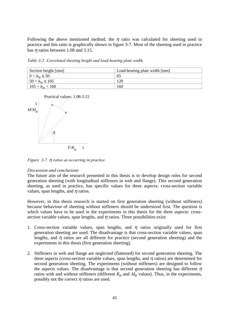
45
Following the above mentioned method, the η ratio was calculated for sheeting used inpractice and this ratio is graphically shown in figure 3-7. Most of the sheeting used in practicehas η ratios between 1.08 and 3.15.
Table 3-2. Correlated sheeting height and load-bearing plate width.
Section height [mm] Load-bearing plate width [mm]0 < hw ≤ 50 6550 < hw ≤ 105 120105 < hw < 160 160
1
1M/Mu
F/Ru
Practical values: 1.08-3.15
η
Figure 3-7. η ratios as occurring in practice.
Discussion and conclusionsThe future aim of the research presented in this thesis is to develop design rules for secondgeneration sheeting (with longitudinal stiffeners in web and flange). This second generationsheeting, as used in practice, has specific values for three aspects: cross-section variablevalues, span lengths, and η ratios.
However, in this thesis research is started on first generation sheeting (without stiffeners)because behaviour of sheeting without stiffeners should be understood first. The question iswhich values have to be used in the experiments in this thesis for the three aspects: cross-section variable values, span lengths, and η ratios. Three possibilities exist:
1. Cross-section variable values, span lengths, and η ratios originally used for firstgeneration sheeting are used. The disadvantage is that cross-section variable values, spanlengths, and η ratios are all different for practice (second generation sheeting) and theexperiments in this thesis (first generation sheeting).
2. Stiffeners in web and flange are neglected (flattened) for second generation sheeting. Thethree aspects (cross-section variable values, span lengths, and η ratios) are determined forsecond generation sheeting. The experiments (without stiffeners) are designed to followthe aspects values. The disadvantage is that second generation sheeting has different ηratios with and without stiffeners (different Ru and Mu values). Thus, in the experiments,possibly not the correct η ratios are used.
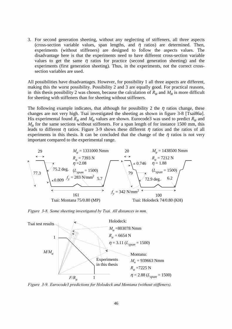
46
3. For second generation sheeting, without any neglecting of stiffeners, all three aspects(cross-section variable values, span lengths, and η ratios) are determined. Then,experiments (without stiffeners) are designed to follow the aspects values. Thedisadvantage here is that the experiments need to have different cross-section variablevalues to get the same η ratios for practice (second generation sheeting) and theexperiments (first generation sheeting). Thus, in the experiments, not the correct cross-section variables are used.
All possibilities have disadvantages. However, for possibility 1 all three aspects are different,making this the worst possibility. Possibility 2 and 3 are equally good. For practical reasons,in this thesis possibility 2 was chosen, because the calculation of Ru and Mu is more difficultfor sheeting with stiffeners than for sheeting without stiffeners.
The following example indicates, that although for possibility 2 the η ratios change, thesechanges are not very high. Tsai investigated the sheeting as shown in figure 3-8 [Tsai86a].His experimental found Ru and Mu values are shown. Eurocode3 was used to predict Ru andMu for the same sections without stiffeners. For a span length of for instance 1500 mm, thisleads to different η ratios. Figure 3-9 shows these different η ratios and the ratios of allexperiments in this thesis. It can be concluded that the change of the η ratios is not veryimportant compared to the experimental range.
100161
2029
72.9 deg.
75.2 deg.
5.7 6.277.3 79
Tsai: Holodeck 74/0.80 (KH)Tsai: Montana 75/0.80 (MP)
0.809
0.746
fy = 283 N/mm2
fy = 342 N/mm2
Mu = 1331000 Nmm
Ru = 7393 Nη =2.08
(Lspan = 1500)
Mu = 1438500 Nmm
Ru = 7212 Nη = 1.88
(Lspan = 1500)
Figure 3-8. Some sheeting investigated by Tsai. All distances in mm.
M/Mu
F/Ru
1
1
Experimentsin this thesis
Montana:Mu = 939663 Nmm
Ru =7225 N
η = 2.88 (Lspan = 1500)
Holodeck:
Mu =803078 Nmm
Ru = 6654 N
η = 3.11 (Lspan = 1500)
Tsai test results
Figure 3-9. Eurocode3 predictions for Holodeck and Montana (without stiffeners).
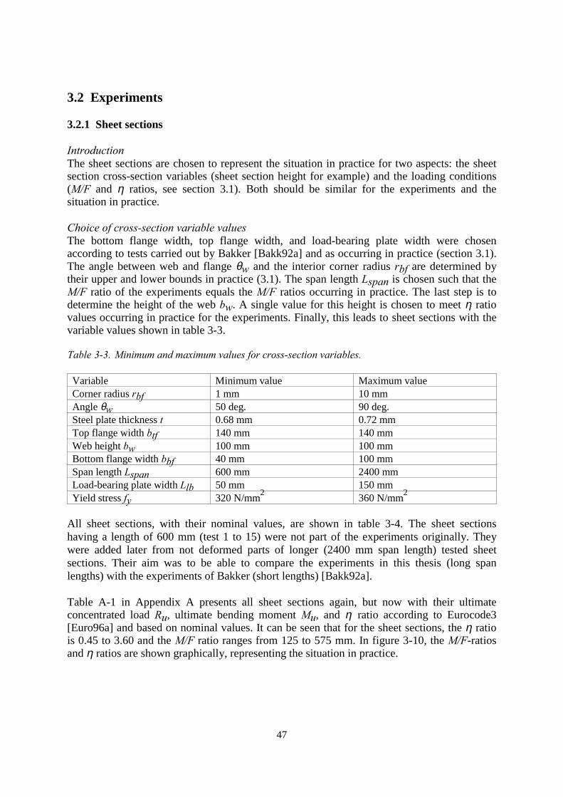
47
3.2 Experiments
3.2.1 Sheet sections
IntroductionThe sheet sections are chosen to represent the situation in practice for two aspects: the sheetsection cross-section variables (sheet section height for example) and the loading conditions(M/F and η ratios, see section 3.1). Both should be similar for the experiments and thesituation in practice.
Choice of cross-section variable valuesThe bottom flange width, top flange width, and load-bearing plate width were chosenaccording to tests carried out by Bakker [Bakk92a] and as occurring in practice (section 3.1).The angle between web and flange θw and the interior corner radius rbf are determined bytheir upper and lower bounds in practice (3.1). The span length Lspan is chosen such that theM/F ratio of the experiments equals the M/F ratios occurring in practice. The last step is todetermine the height of the web bw. A single value for this height is chosen to meet η ratiovalues occurring in practice for the experiments. Finally, this leads to sheet sections with thevariable values shown in table 3-3.
Table 3-3. Minimum and maximum values for cross-section variables.
Variable Minimum value Maximum valueCorner radius rbf 1 mm 10 mmAngle θw 50 deg. 90 deg.Steel plate thickness t 0.68 mm 0.72 mmTop flange width btf 140 mm 140 mmWeb height bw 100 mm 100 mmBottom flange width bbf 40 mm 100 mmSpan length Lspan 600 mm 2400 mmLoad-bearing plate width Llb 50 mm 150 mmYield stress fy 320 N/mm2 360 N/mm2
All sheet sections, with their nominal values, are shown in table 3-4. The sheet sectionshaving a length of 600 mm (test 1 to 15) were not part of the experiments originally. Theywere added later from not deformed parts of longer (2400 mm span length) tested sheetsections. Their aim was to be able to compare the experiments in this thesis (long spanlengths) with the experiments of Bakker (short lengths) [Bakk92a].
Table A-1 in Appendix A presents all sheet sections again, but now with their ultimateconcentrated load Ru, ultimate bending moment Mu, and η ratio according to Eurocode3[Euro96a] and based on nominal values. It can be seen that for the sheet sections, the η ratiois 0.45 to 3.60 and the M/F ratio ranges from 125 to 575 mm. In figure 3-10, the M/F-ratiosand η ratios are shown graphically, representing the situation in practice.
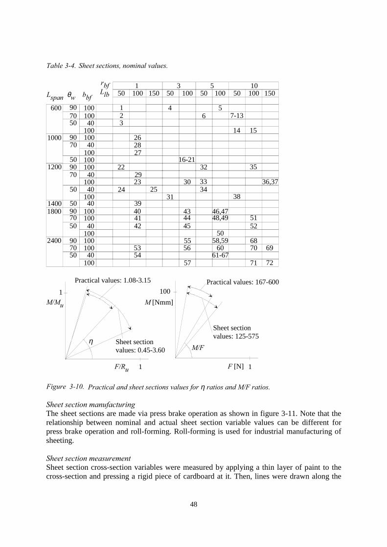
48
Table 3-4. Sheet sections, nominal values.
Lspan θw bbf
rbfLlb 50 100 150
150 100
350 100
550 100 150
10
70
50
50
7090
50
1200
14001800
24007090
50
2430
100
10040
40100100
10040
10040
100100
25
29
31
3334
36,37
4241
38
43 46,4739
44 48,49 5140
45 5250
5354
5556
57
58,5960
61-67
23
686970
71 72
40
70 100 290
50
600 1
3
4 57-13
15
100
1440
100
6
5090
1000
27
35100100
16-21
26
22 32
289070
100
10040
1
1
1
100M [Nmm]
F [N]
M/Mu
F/Ru
Practical values: 167-600Practical values: 1.08-3.15
Sheet sectionvalues: 0.45-3.60
Sheet sectionvalues: 125-575
ηM/F
Figure 3-10. Practical and sheet sections values for η ratios and M/F ratios.
Sheet section manufacturingThe sheet sections are made via press brake operation as shown in figure 3-11. Note that therelationship between nominal and actual sheet section variable values can be different forpress brake operation and roll-forming. Roll-forming is used for industrial manufacturing ofsheeting.
Sheet section measurementSheet section cross-section variables were measured by applying a thin layer of paint to thecross-section and pressing a rigid piece of cardboard at it. Then, lines were drawn along the
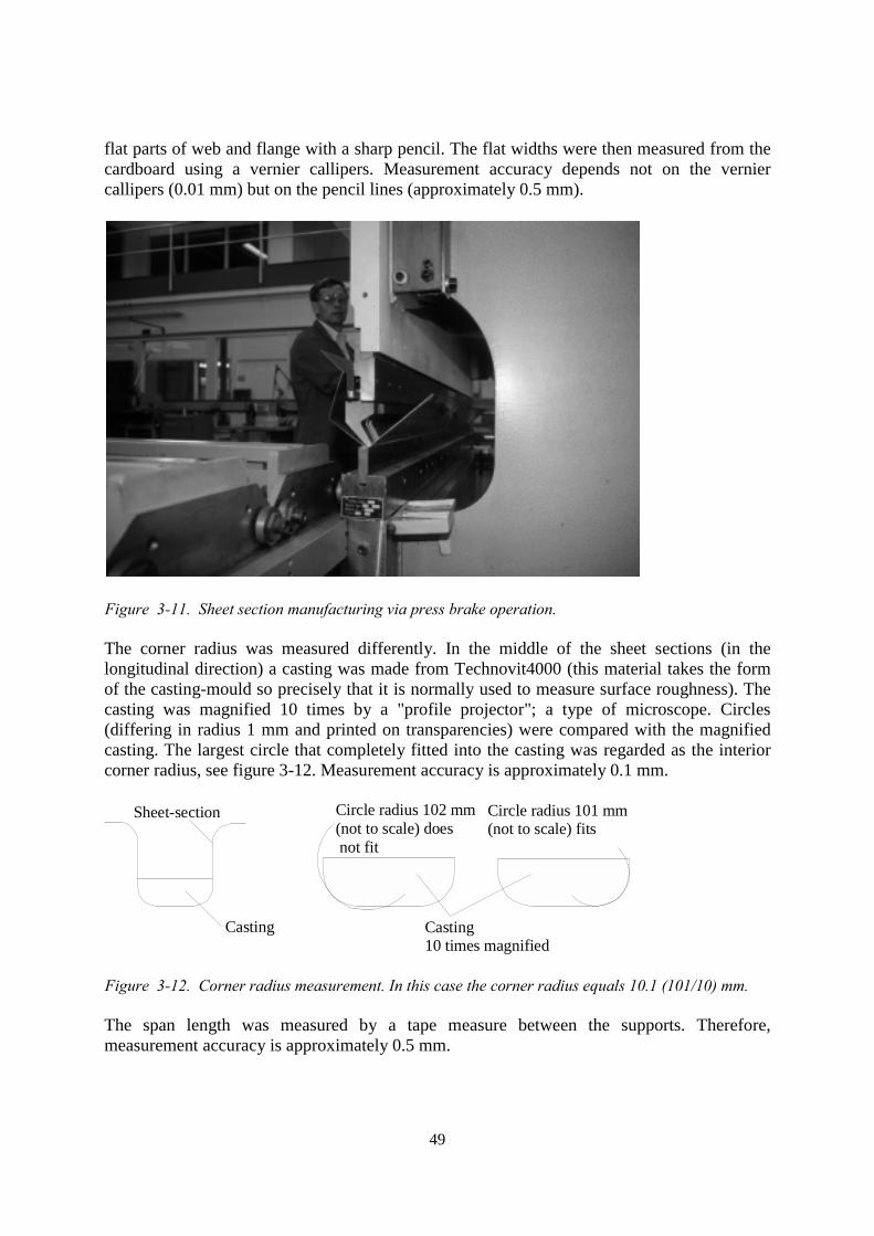
49
flat parts of web and flange with a sharp pencil. The flat widths were then measured from thecardboard using a vernier callipers. Measurement accuracy depends not on the verniercallipers (0.01 mm) but on the pencil lines (approximately 0.5 mm).
Figure 3-11. Sheet section manufacturing via press brake operation.
The corner radius was measured differently. In the middle of the sheet sections (in thelongitudinal direction) a casting was made from Technovit4000 (this material takes the formof the casting-mould so precisely that it is normally used to measure surface roughness). Thecasting was magnified 10 times by a "profile projector"; a type of microscope. Circles(differing in radius 1 mm and printed on transparencies) were compared with the magnifiedcasting. The largest circle that completely fitted into the casting was regarded as the interiorcorner radius, see figure 3-12. Measurement accuracy is approximately 0.1 mm.
Sheet-section
Casting
Circle radius 102 mm(not to scale) does not fit
Circle radius 101 mm(not to scale) fits
Casting10 times magnified
Figure 3-12. Corner radius measurement. In this case the corner radius equals 10.1 (101/10) mm.
The span length was measured by a tape measure between the supports. Therefore,measurement accuracy is approximately 0.5 mm.
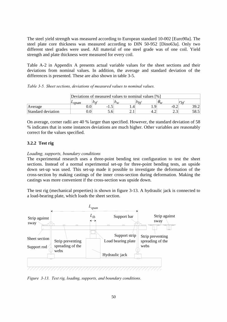
50
The steel yield strength was measured according to European standard 10-002 [Euro90a]. Thesteel plate core thickness was measured according to DIN 50-952 [Dino63a]. Only twodifferent steel grades were used. All material of one steel grade was of one coil. Yieldstrength and plate thickness were measured for every coil.
Table A-2 in Appendix A presents actual variable values for the sheet sections and theirdeviations from nominal values. In addition, the average and standard deviation of thedifferences is presented. These are also shown in table 3-5.
Table 3-5. Sheet sections, deviations of measured values to nominal values.
Deviations of measured values to nominal values [%]Lspan btf bw bbf θw rbf
Average 0.0 -1.5 1.4 1.9 -0.2 39.2Standard deviation 0.0 5.6 2.1 4.2 2.3 58.5
On average, corner radii are 40 % larger than specified. However, the standard deviation of 58% indicates that in some instances deviations are much higher. Other variables are reasonablycorrect for the values specified.
3.2.2 Test rig
Loading, supports, boundary conditionsThe experimental research uses a three-point bending test configuration to test the sheetsections. Instead of a normal experimental set-up for three-point bending tests, an upsidedown set-up was used. This set-up made it possible to investigate the deformation of thecross-section by making castings of the inner cross-section during deformation. Making thecastings was more convenient if the cross-section was upside down.
The test rig (mechanical properties) is shown in figure 3-13. A hydraulic jack is connected toa load-bearing plate, which loads the sheet section.
Support rod
Support stripLoad bearing plateSheet section Strip preventing
spreading of the webs
Strip againstsway
Hydraulic jack
Support bar
Strip preventingspreading of the webs
Strip againstsway
Lspan
Llb
Figure 3-13. Test rig, loading, supports, and boundary conditions.
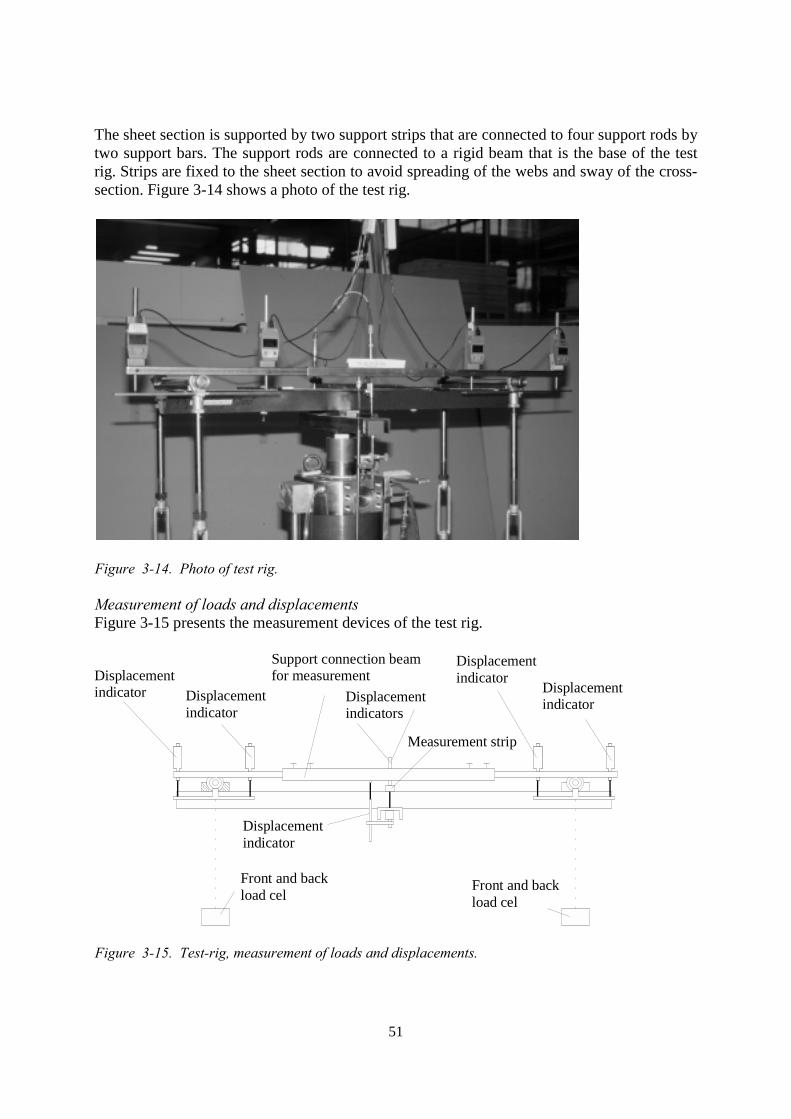
51
The sheet section is supported by two support strips that are connected to four support rods bytwo support bars. The support rods are connected to a rigid beam that is the base of the testrig. Strips are fixed to the sheet section to avoid spreading of the webs and sway of the cross-section. Figure 3-14 shows a photo of the test rig.
Figure 3-14. Photo of test rig.
Measurement of loads and displacementsFigure 3-15 presents the measurement devices of the test rig.
Measurement strip
Support connection beamfor measurement
Front and backload cel
Front and backload cel
Displacementindicator Displacement
indicator
Displacementindicator
Displacementindicator
Displacementindicator
Displacementindicators
Figure 3-15. Test-rig, measurement of loads and displacements.
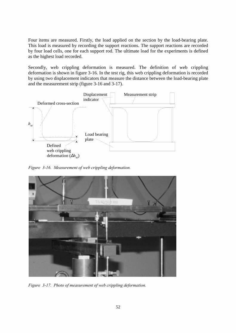
52
Four items are measured. Firstly, the load applied on the section by the load-bearing plate.This load is measured by recording the support reactions. The support reactions are recordedby four load cells, one for each support rod. The ultimate load for the experiments is definedas the highest load recorded.
Secondly, web crippling deformation is measured. The definition of web cripplingdeformation is shown in figure 3-16. In the test rig, this web crippling deformation is recordedby using two displacement indicators that measure the distance between the load-bearing plateand the measurement strip (figure 3-16 and 3-17).
deformation (∆hw)
Deformed cross-section
hw
Definedweb crippling
Load bearingplate
Measurement stripDisplacementindicator
Figure 3-16. Measurement of web crippling deformation.
Figure 3-17. Photo of measurement of web crippling deformation.
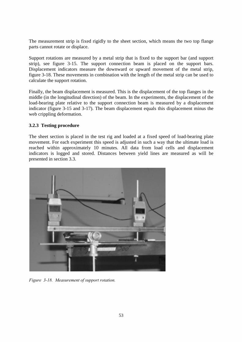
53
The measurement strip is fixed rigidly to the sheet section, which means the two top flangeparts cannot rotate or displace.
Support rotations are measured by a metal strip that is fixed to the support bar (and supportstrip), see figure 3-15. The support connection beam is placed on the support bars.Displacement indicators measure the downward or upward movement of the metal strip,figure 3-18. These movements in combination with the length of the metal strip can be used tocalculate the support rotation.
Finally, the beam displacement is measured. This is the displacement of the top flanges in themiddle (in the longitudinal direction) of the beam. In the experiments, the displacement of theload-bearing plate relative to the support connection beam is measured by a displacementindicator (figure 3-15 and 3-17). The beam displacement equals this displacement minus theweb crippling deformation.
3.2.3 Testing procedure
The sheet section is placed in the test rig and loaded at a fixed speed of load-bearing platemovement. For each experiment this speed is adjusted in such a way that the ultimate load isreached within approximately 10 minutes. All data from load cells and displacementindicators is logged and stored. Distances between yield lines are measured as will bepresented in section 3.3.
Figure 3-18. Measurement of support rotation.
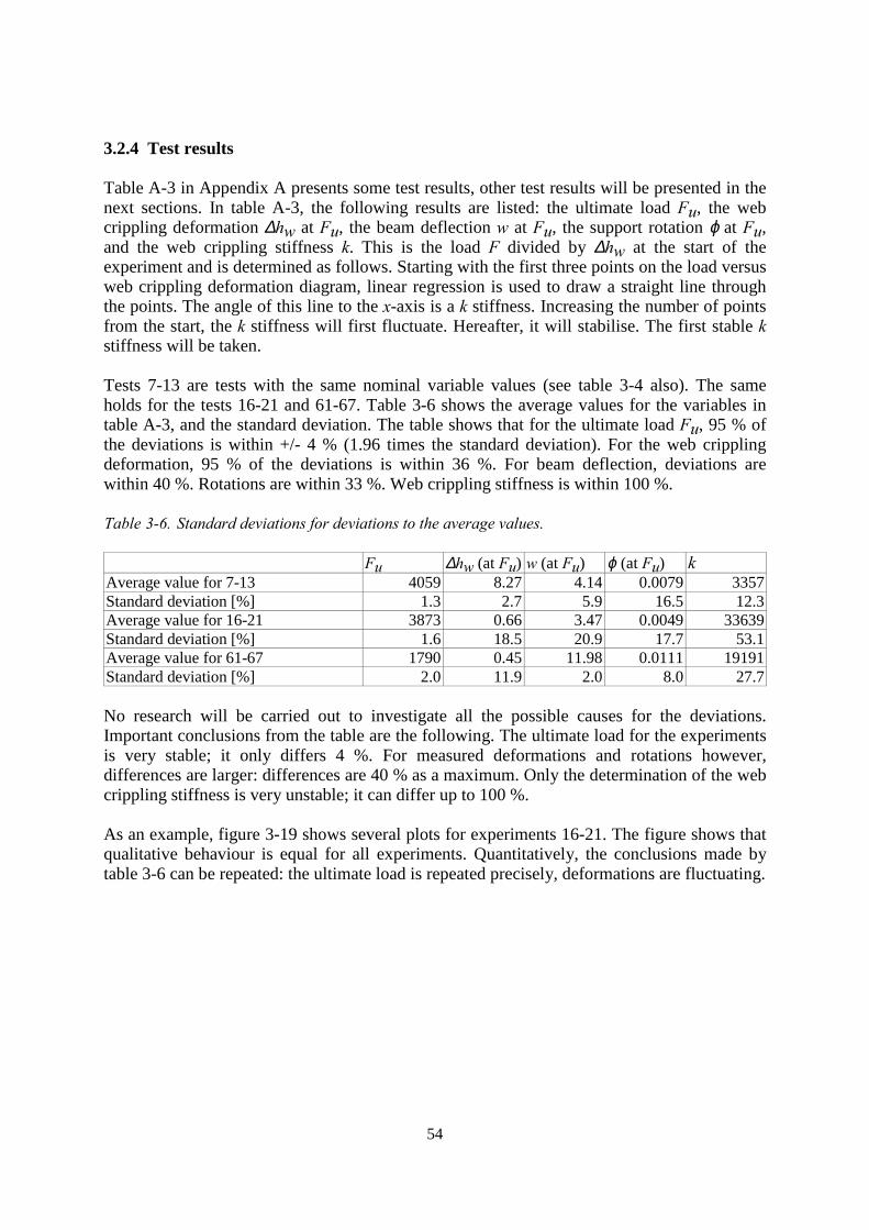
54
3.2.4 Test results
Table A-3 in Appendix A presents some test results, other test results will be presented in thenext sections. In table A-3, the following results are listed: the ultimate load Fu, the webcrippling deformation ∆hw at Fu, the beam deflection w at Fu, the support rotation ϕ at Fu,and the web crippling stiffness k. This is the load F divided by ∆hw at the start of theexperiment and is determined as follows. Starting with the first three points on the load versusweb crippling deformation diagram, linear regression is used to draw a straight line throughthe points. The angle of this line to the x-axis is a k stiffness. Increasing the number of pointsfrom the start, the k stiffness will first fluctuate. Hereafter, it will stabilise. The first stable kstiffness will be taken.
Tests 7-13 are tests with the same nominal variable values (see table 3-4 also). The sameholds for the tests 16-21 and 61-67. Table 3-6 shows the average values for the variables intable A-3, and the standard deviation. The table shows that for the ultimate load Fu, 95 % ofthe deviations is within +/- 4 % (1.96 times the standard deviation). For the web cripplingdeformation, 95 % of the deviations is within 36 %. For beam deflection, deviations arewithin 40 %. Rotations are within 33 %. Web crippling stiffness is within 100 %.
Table 3-6. Standard deviations for deviations to the average values.
Fu ∆hw (at Fu) w (at Fu) ϕ (at Fu) kAverage value for 7-13 4059 8.27 4.14 0.0079 3357Standard deviation [%] 1.3 2.7 5.9 16.5 12.3Average value for 16-21 3873 0.66 3.47 0.0049 33639Standard deviation [%] 1.6 18.5 20.9 17.7 53.1Average value for 61-67 1790 0.45 11.98 0.0111 19191Standard deviation [%] 2.0 11.9 2.0 8.0 27.7
No research will be carried out to investigate all the possible causes for the deviations.Important conclusions from the table are the following. The ultimate load for the experimentsis very stable; it only differs 4 %. For measured deformations and rotations however,differences are larger: differences are 40 % as a maximum. Only the determination of the webcrippling stiffness is very unstable; it can differ up to 100 %.
As an example, figure 3-19 shows several plots for experiments 16-21. The figure shows thatqualitative behaviour is equal for all experiments. Quantitatively, the conclusions made bytable 3-6 can be repeated: the ultimate load is repeated precisely, deformations are fluctuating.
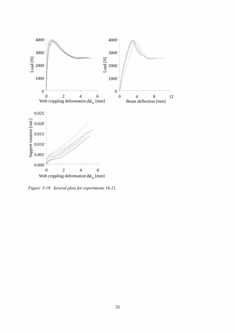
55
0 2 4 6Web crippling deformation ∆hw [mm]
0
1000
2000
3000
4000
Load
[N]
0 4 8 12Beam deflection [mm]
0
1000
2000
3000
4000
Load
[N]
0 2 4 60.000
0.005
0.010
0.015
0.020
0.025
Supp
ort r
otat
ion
[rad
.]
Web crippling deformation ∆hw [mm]
Figure 3-19. Several plots for experiments 16-21.
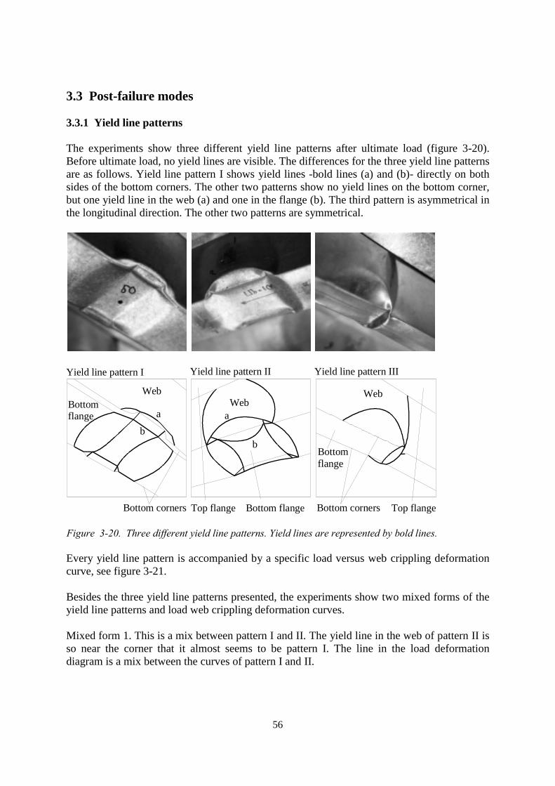
56
3.3 Post-failure modes
3.3.1 Yield line patterns
The experiments show three different yield line patterns after ultimate load (figure 3-20).Before ultimate load, no yield lines are visible. The differences for the three yield line patternsare as follows. Yield line pattern I shows yield lines -bold lines (a) and (b)- directly on bothsides of the bottom corners. The other two patterns show no yield lines on the bottom corner,but one yield line in the web (a) and one in the flange (b). The third pattern is asymmetrical inthe longitudinal direction. The other two patterns are symmetrical.
WebBottomflange
Bottom corners
Web
Bottom flangeTop flange
Web
Bottomflange
Top flangeBottom corners
Yield line pattern I Yield line pattern II Yield line pattern III
a
bb
a
Figure 3-20. Three different yield line patterns. Yield lines are represented by bold lines.
Every yield line pattern is accompanied by a specific load versus web crippling deformationcurve, see figure 3-21.
Besides the three yield line patterns presented, the experiments show two mixed forms of theyield line patterns and load web crippling deformation curves.
Mixed form 1. This is a mix between pattern I and II. The yield line in the web of pattern II isso near the corner that it almost seems to be pattern I. The line in the load deformationdiagram is a mix between the curves of pattern I and II.
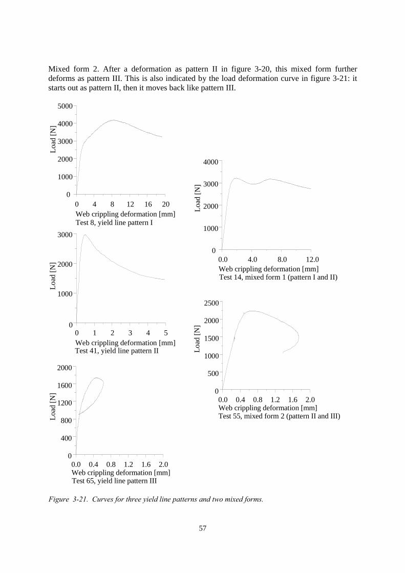
57
Mixed form 2. After a deformation as pattern II in figure 3-20, this mixed form furtherdeforms as pattern III. This is also indicated by the load deformation curve in figure 3-21: itstarts out as pattern II, then it moves back like pattern III.
0 4 8 12 16 20Web crippling deformation [mm]Test 8, yield line pattern I
0
1000
2000
3000
4000
5000
Load
[N]
0 1 2 3 4 5Web crippling deformation [mm]Test 41, yield line pattern II
0
1000
2000
3000
0.0 4.0 8.0 12.0Web crippling deformation [mm]Test 14, mixed form 1 (pattern I and II)
0
1000
2000
3000
4000
0.0 0.4 0.8 1.2 1.6 2.0Web crippling deformation [mm]Test 65, yield line pattern III
0
400
800
1200
1600
2000
0.0 0.4 0.8 1.2 1.6 2.0Web crippling deformation [mm]Test 55, mixed form 2 (pattern II and III)
0
500
1000
1500
2000
2500
Load
[N]
Load
[N]
Load
[N]
Load
[N]
Figure 3-21. Curves for three yield line patterns and two mixed forms.
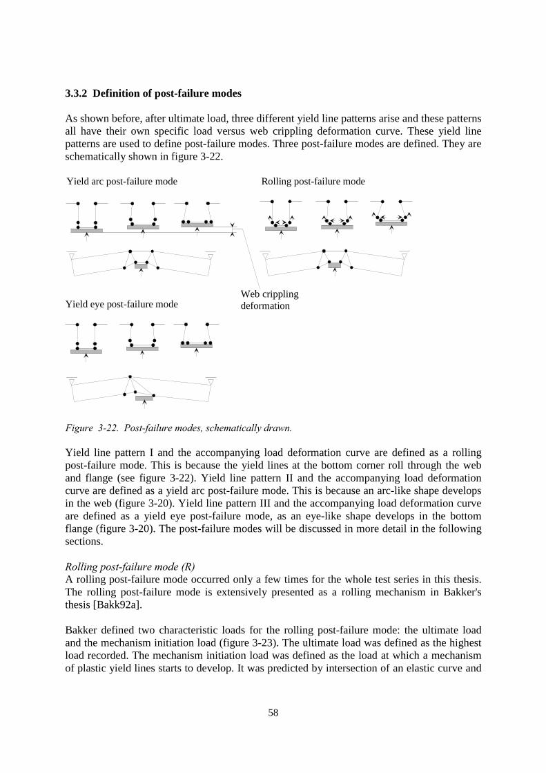
58
3.3.2 Definition of post-failure modes
As shown before, after ultimate load, three different yield line patterns arise and these patternsall have their own specific load versus web crippling deformation curve. These yield linepatterns are used to define post-failure modes. Three post-failure modes are defined. They areschematically shown in figure 3-22.
Yield arc post-failure mode Rolling post-failure mode
Yield eye post-failure modeWeb cripplingdeformation
Figure 3-22. Post-failure modes, schematically drawn.
Yield line pattern I and the accompanying load deformation curve are defined as a rollingpost-failure mode. This is because the yield lines at the bottom corner roll through the weband flange (see figure 3-22). Yield line pattern II and the accompanying load deformationcurve are defined as a yield arc post-failure mode. This is because an arc-like shape developsin the web (figure 3-20). Yield line pattern III and the accompanying load deformation curveare defined as a yield eye post-failure mode, as an eye-like shape develops in the bottomflange (figure 3-20). The post-failure modes will be discussed in more detail in the followingsections.
Rolling post-failure mode (R)A rolling post-failure mode occurred only a few times for the whole test series in this thesis.The rolling post-failure mode is extensively presented as a rolling mechanism in Bakker'sthesis [Bakk92a].
Bakker defined two characteristic loads for the rolling post-failure mode: the ultimate loadand the mechanism initiation load (figure 3-23). The ultimate load was defined as the highestload recorded. The mechanism initiation load was defined as the load at which a mechanismof plastic yield lines starts to develop. It was predicted by intersection of an elastic curve and
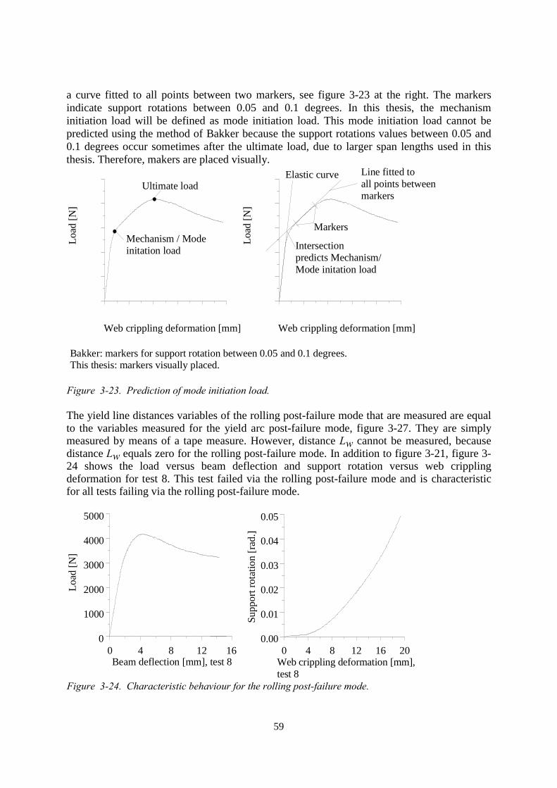
59
a curve fitted to all points between two markers, see figure 3-23 at the right. The markersindicate support rotations between 0.05 and 0.1 degrees. In this thesis, the mechanisminitiation load will be defined as mode initiation load. This mode initiation load cannot bepredicted using the method of Bakker because the support rotations values between 0.05 and0.1 degrees occur sometimes after the ultimate load, due to larger span lengths used in thisthesis. Therefore, makers are placed visually.
Web crippling deformation [mm]
Load
[N]
Elastic curve Line fitted toall points betweenmarkers
Intersectionpredicts Mechanism/Mode initation load
Web crippling deformation [mm]
Load
[N]
Mechanism / Modeinitation load
Ultimate load
Markers
Bakker: markers for support rotation between 0.05 and 0.1 degrees.This thesis: markers visually placed.
Figure 3-23. Prediction of mode initiation load.
The yield line distances variables of the rolling post-failure mode that are measured are equalto the variables measured for the yield arc post-failure mode, figure 3-27. They are simplymeasured by means of a tape measure. However, distance Lw cannot be measured, becausedistance Lw equals zero for the rolling post-failure mode. In addition to figure 3-21, figure 3-24 shows the load versus beam deflection and support rotation versus web cripplingdeformation for test 8. This test failed via the rolling post-failure mode and is characteristicfor all tests failing via the rolling post-failure mode.
0 4 8 12 16 20Web crippling deformation [mm],test 8
0.00
0.01
0.02
0.03
0.04
0.05
0 4 8 12 16Beam deflection [mm], test 8
0
1000
2000
3000
4000
5000
Supp
ort r
otat
ion
[rad
.]
Load
[N]
Figure 3-24. Characteristic behaviour for the rolling post-failure mode.
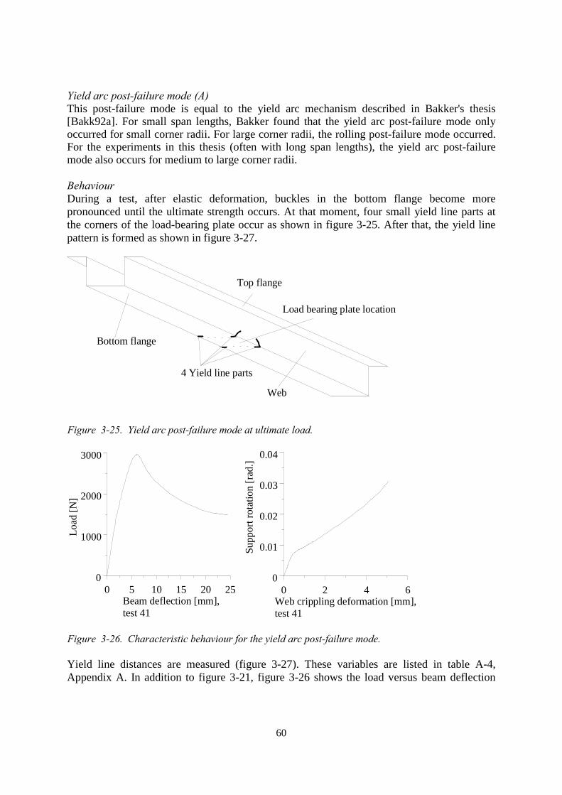
60
Yield arc post-failure mode (A)This post-failure mode is equal to the yield arc mechanism described in Bakker's thesis[Bakk92a]. For small span lengths, Bakker found that the yield arc post-failure mode onlyoccurred for small corner radii. For large corner radii, the rolling post-failure mode occurred.For the experiments in this thesis (often with long span lengths), the yield arc post-failuremode also occurs for medium to large corner radii.
BehaviourDuring a test, after elastic deformation, buckles in the bottom flange become morepronounced until the ultimate strength occurs. At that moment, four small yield line parts atthe corners of the load-bearing plate occur as shown in figure 3-25. After that, the yield linepattern is formed as shown in figure 3-27.
Bottom flange
Top flange
4 Yield line parts
Load bearing plate location
Web
Figure 3-25. Yield arc post-failure mode at ultimate load.
0 5 10 15 20 25Beam deflection [mm],test 41
0
1000
2000
3000
0 2 4 6Web crippling deformation [mm],test 41
0
0.01
0.02
0.03
0.04
Load
[N]
Supp
ort r
otat
ion
[rad
.]
Figure 3-26. Characteristic behaviour for the yield arc post-failure mode.
Yield line distances are measured (figure 3-27). These variables are listed in table A-4,Appendix A. In addition to figure 3-21, figure 3-26 shows the load versus beam deflection
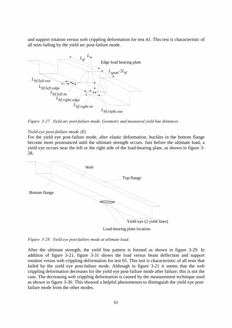
61
and support rotation versus web crippling deformation for test 41. This test is characteristic ofall tests failing by the yield arc post-failure mode.
Edge load bearing plateLwLtf
Lspan-2LtfLbf;left;out
Lbf;left;edgeLbf;left;in
Lbf;right;edgeLbf;right;in
Lbf;right;out
Figure 3-27. Yield arc post-failure mode. Geometry and measured yield line distances.
Yield eye post-failure mode (E)For the yield eye post-failure mode, after elastic deformation, buckles in the bottom flangebecome more pronounced until the ultimate strength occurs. Just before the ultimate load, ayield eye occurs near the left or the right side of the load-bearing plate, as shown in figure 3-28.
Top flange
Bottom flange
Yield eye (2 yield lines)
Load-bearing plate location
Web
Figure 3-28. Yield eye post-failure mode at ultimate load.
After the ultimate strength, the yield line pattern is formed as shown in figure 3-29. Inaddition of figure 3-21, figure 3-31 shows the load versus beam deflection and supportrotation versus web crippling deformation for test 65. This test is characteristic of all tests thatfailed by the yield eye post-failure mode. Although in figure 3-21 it seems that the webcrippling deformation decreases for the yield eye post-failure mode after failure, this is not thecase. The decreasing web crippling deformation is caused by the measurement technique usedas shown in figure 3-30. This showed a helpful phenomenon to distinguish the yield eye post-failure mode from the other modes.
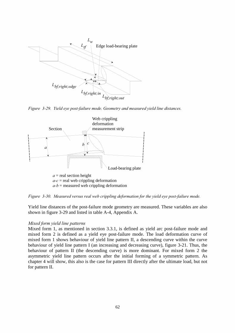
62
Edge load-bearing plateLw
Ltf
Lbf;right;edge
Lbf;right;outLbf;right;in
Figure 3-29. Yield eye post-failure mode. Geometry and measured yield line distances.
a b c
a = real section heighta-c = real web crippling deformationa-b = measured web crippling deformation
Section
Load-bearing plate
Web cripplingdeformation measurement strip
Figure 3-30. Measured versus real web crippling deformation for the yield eye post-failure mode.
Yield line distances of the post-failure mode geometry are measured. These variables are alsoshown in figure 3-29 and listed in table A-4, Appendix A.
Mixed form yield line patternsMixed form 1, as mentioned in section 3.3.1, is defined as yield arc post-failure mode andmixed form 2 is defined as a yield eye post-failure mode. The load deformation curve ofmixed form 1 shows behaviour of yield line pattern II, a descending curve within the curvebehaviour of yield line pattern I (an increasing and decreasing curve), figure 3-21. Thus, thebehaviour of pattern II (the descending curve) is more dominant. For mixed form 2 theasymmetric yield line pattern occurs after the initial forming of a symmetric pattern. Aschapter 4 will show, this also is the case for pattern III directly after the ultimate load, but notfor pattern II.
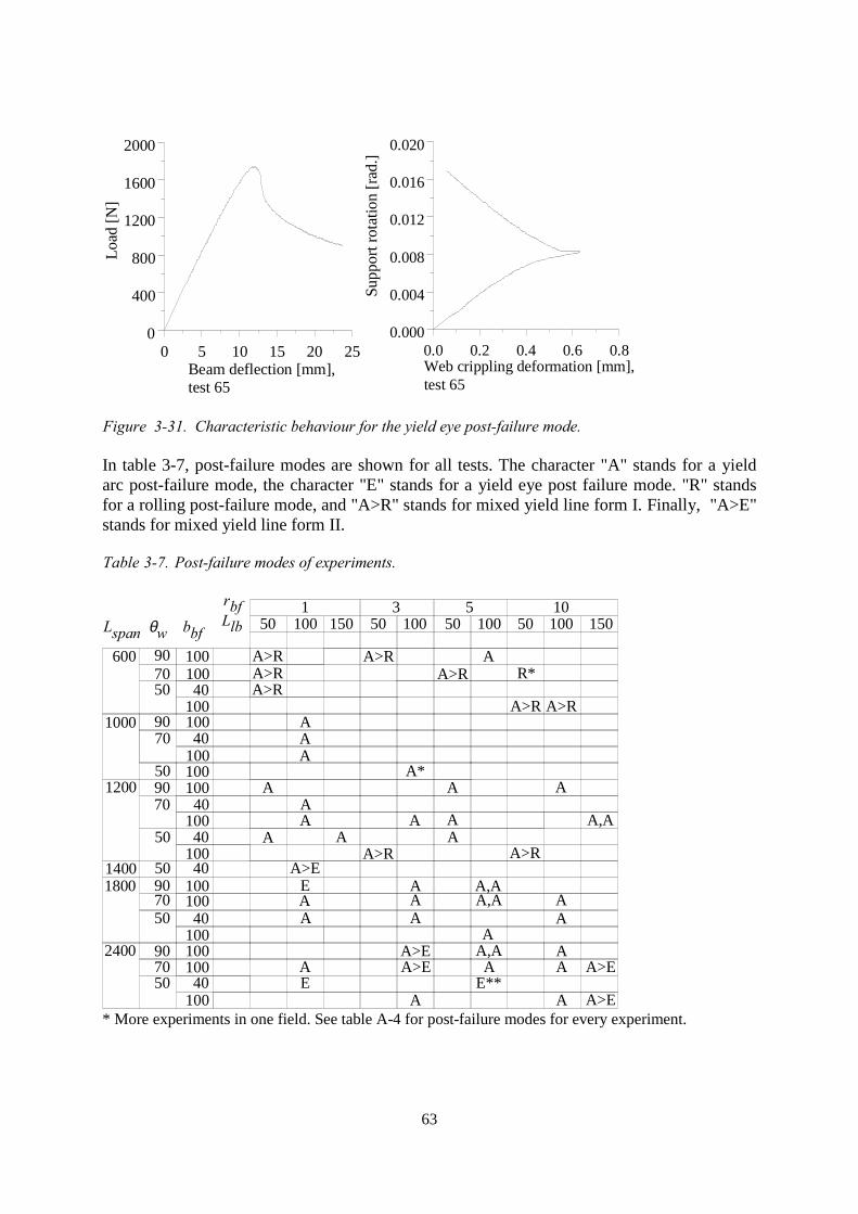
63
0 5 10 15 20 25Beam deflection [mm],test 65
0
400
800
1200
1600
2000
0.0 0.2 0.4 0.6 0.8Web crippling deformation [mm],test 65
0.000
0.004
0.008
0.012
0.016
0.020
Load
[N]
Supp
ort r
otat
ion
[rad
.]
Figure 3-31. Characteristic behaviour for the yield eye post-failure mode.
In table 3-7, post-failure modes are shown for all tests. The character "A" stands for a yieldarc post-failure mode, the character "E" stands for a yield eye post failure mode. "R" standsfor a rolling post-failure mode, and "A>R" stands for mixed yield line form I. Finally, "A>E"stands for mixed yield line form II.
Table 3-7. Post-failure modes of experiments.
Lspan θw bbf
rbfLlb 50 100 150
150 100
350 100
550 100 150
10
70
50
50
7090
50
1200
14001800
24007090
50
AA
100
10040
40100100
10040
10040
100100
A
A
A>R
AA
A,A
AA
A>R
A A,AA>E
A A,A AE
A AA
AE
A>EA>E
A
A,AA
E**
A
AA>EA
A A>E
40
70 100 A>R90
50
600 A>R
A>R
A>R AR*
A>R
100
A>R40
100
A>R
5090
1000
A
A100100
A*
A
A A
A9070
100
10040
* More experiments in one field. See table A-4 for post-failure modes for every experiment.

64
3.3.3 Relevance rolling post-failure mode
Table 3-7 shows that the rolling post-failure mode only occurs for a span length equal to 600mm. Experiments with this span length do not simulate a practical situation but their aim is tocompare the experiments in this thesis (long span lengths) with the experiments of Bakker[Bakk92a] (short lengths), see section 3.2.1. Furthermore, chapter 4 will show that the rollingpost-failure mode can occur for long span lengths, but only for very small, unrealistic load-bearing plate widths (25 mm). As a conclusion, the rolling post-failure mode does not occurfor practical situations. Thus, only the yield arc and yield eye post-failure modes are relevant.

65
3.4 Conclusions
Three-point bending tests on sheet sections were carried out. These tests simulate the practicalapplication and loading of first-generation sheeting.
A new method was developed to measure the interior corner radius to 0.1 mm accuracy.
The experiments show three distinct yield line patterns after ultimate load. These yield linepatterns all have a distinct load deformation curve. Furthermore, there are two mixed yieldline patterns that have a mixed load deformation curve too.
The yield line patterns and load deformation curves are used for a definition of three post-failure modes: the rolling, yield arc, and yield eye post-failure modes. The mixed yield linepatterns are grouped into these three post-failure modes.
For practical situations, the rolling post-failure mode is not relevant. Only the yield arc andyield eye post-failure modes are relevant.

66
4 Finite element models
Chapter abstractThree different finite element models are presented, one for each post-failure mode found inchapter 3. The finite element models are used to simulate some of the experiments in chapter3. The finite element models indicate that threre are only two ultimate failure modes for theexperiments until and at ultimate load. The reliability of the finite element models is checkedby two special series of simulations.
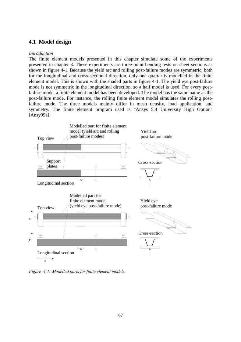
67
4.1 Model design
IntroductionThe finite element models presented in this chapter simulate some of the experimentspresented in chapter 3. These experiments are three-point bending tests on sheet sections asshown in figure 4-1. Because the yield arc and rolling post-failure modes are symmetric, bothfor the longitudinal and cross-sectional direction, only one quarter is modelled in the finiteelement model. This is shown with the shaded parts in figure 4-1. The yield eye post-failuremode is not symmetric in the longitudinal direction, so a half model is used. For every post-failure mode, a finite element model has been developed. The model has the same name as thepost-failure mode. For instance, the rolling finite element model simulates the rolling post-failure mode. The three models mainly differ in mesh density, load application, andsymmetry. The finite element program used is "Ansys 5.4 University High Option"[Ansy99a].
Longitudinal section
Top view
Cross-section
Modelled part for finite elementmodel (yield arc and rollingpost-failure modes)
Longitudinal section
Top view
Cross-section
Modelled part forfinite element model(yield eye post-failure mode)
Yield arc post-failure mode
Yield eyepost-failure mode
x
y
z
Supportplates
Figure 4-1. Modelled parts for finite element models.
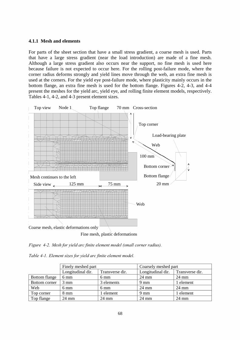
68
4.1.1 Mesh and elements
For parts of the sheet section that have a small stress gradient, a coarse mesh is used. Partsthat have a large stress gradient (near the load introduction) are made of a fine mesh.Although a large stress gradient also occurs near the support, no fine mesh is used herebecause failure is not expected to occur here. For the rolling post-failure mode, where thecorner radius deforms strongly and yield lines move through the web, an extra fine mesh isused at the corners. For the yield eye post-failure mode, where plasticity mainly occurs in thebottom flange, an extra fine mesh is used for the bottom flange. Figures 4-2, 4-3, and 4-4present the meshes for the yield arc, yield eye, and rolling finite element models, respectively.Tables 4-1, 4-2, and 4-3 present element sizes.
Top view
Side viewMesh continues to the left
Coarse mesh, elastic deformations onlyFine mesh, plastic deformations
Web
Cross-sectionTop flange
Top corner
Web
Bottom corner
Bottom flange
Load-bearing plate
20 mm
100 mm
70 mm
75 mm125 mm
Node 1
Figure 4-2. Mesh for yield arc finite element model (small corner radius).
Table 4-1. Element sizes for yield arc finite element model.
Finely meshed part Coarsely meshed partLongitudinal dir. Transverse dir. Longitudinal dir. Transverse dir.
Bottom flange 6 mm 6 mm 24 mm 24 mmBottom corner 3 mm 3 elements 9 mm 1 elementWeb 6 mm 6 mm 24 mm 24 mmTop corner 8 mm 1 element 9 mm 1 elementTop flange 24 mm 24 mm 24 mm 24 mm
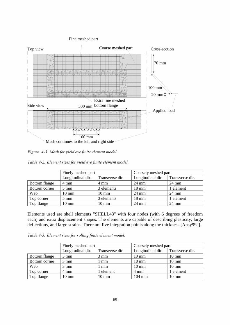
69
Top view
Side view
Cross-section
Applied load
Mesh continues to the left and right side
Fine meshed part
Coarse meshed part
Extra fine meshedbottom flange
20 mm100 mm
70 mm
100 mm
300 mm
Figure 4-3. Mesh for yield eye finite element model.
Table 4-2. Element sizes for yield eye finite element model.
Finely meshed part Coarsely meshed partLongitudinal dir. Transverse dir. Longitudinal dir. Transverse dir.
Bottom flange 4 mm 4 mm 24 mm 24 mmBottom corner 5 mm 3 elements 18 mm 1 elementWeb 10 mm 10 mm 24 mm 24 mmTop corner 5 mm 3 elements 18 mm 1 elementTop flange 10 mm 10 mm 24 mm 24 mm
Elements used are shell elements "SHELL43" with four nodes (with 6 degrees of freedomeach) and extra displacement shapes. The elements are capable of describing plasticity, largedeflections, and large strains. There are five integration points along the thickness [Ansy99a].
Table 4-3. Element sizes for rolling finite element model.
Finely meshed part Coarsely meshed partLongitudinal dir. Transverse dir. Longitudinal dir. Transverse dir.
Bottom flange 3 mm 3 mm 10 mm 10 mmBottom corner 3 mm 1 mm 10 mm 10 mmWeb 3 mm 1 mm 10 mm 10 mmTop corner 4 mm 1 element 4 mm 1 elementTop flange 10 mm 10 mm 104 mm 10 mm
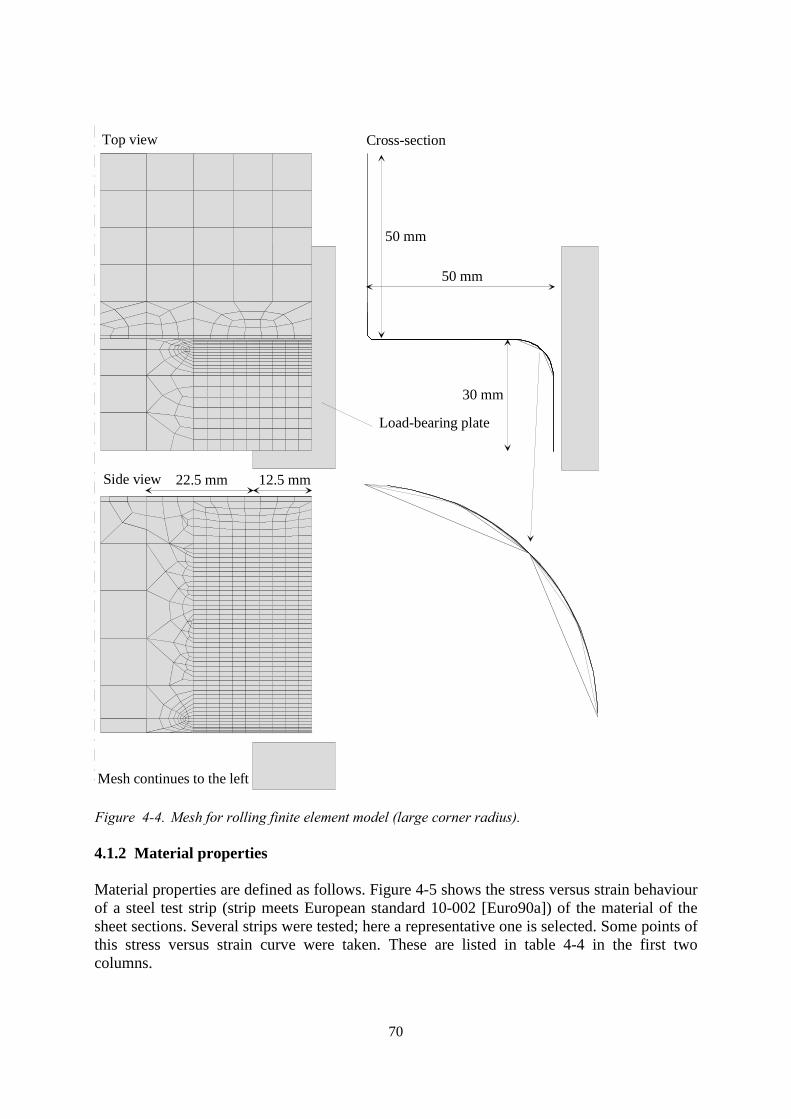
70
Side view
Top view Cross-section
Load-bearing plate
Mesh continues to the left
50 mm
30 mm
50 mm
12.5 mm22.5 mm
Figure 4-4. Mesh for rolling finite element model (large corner radius).
4.1.2 Material properties
Material properties are defined as follows. Figure 4-5 shows the stress versus strain behaviourof a steel test strip (strip meets European standard 10-002 [Euro90a]) of the material of thesheet sections. Several strips were tested; here a representative one is selected. Some points ofthis stress versus strain curve were taken. These are listed in table 4-4 in the first twocolumns.
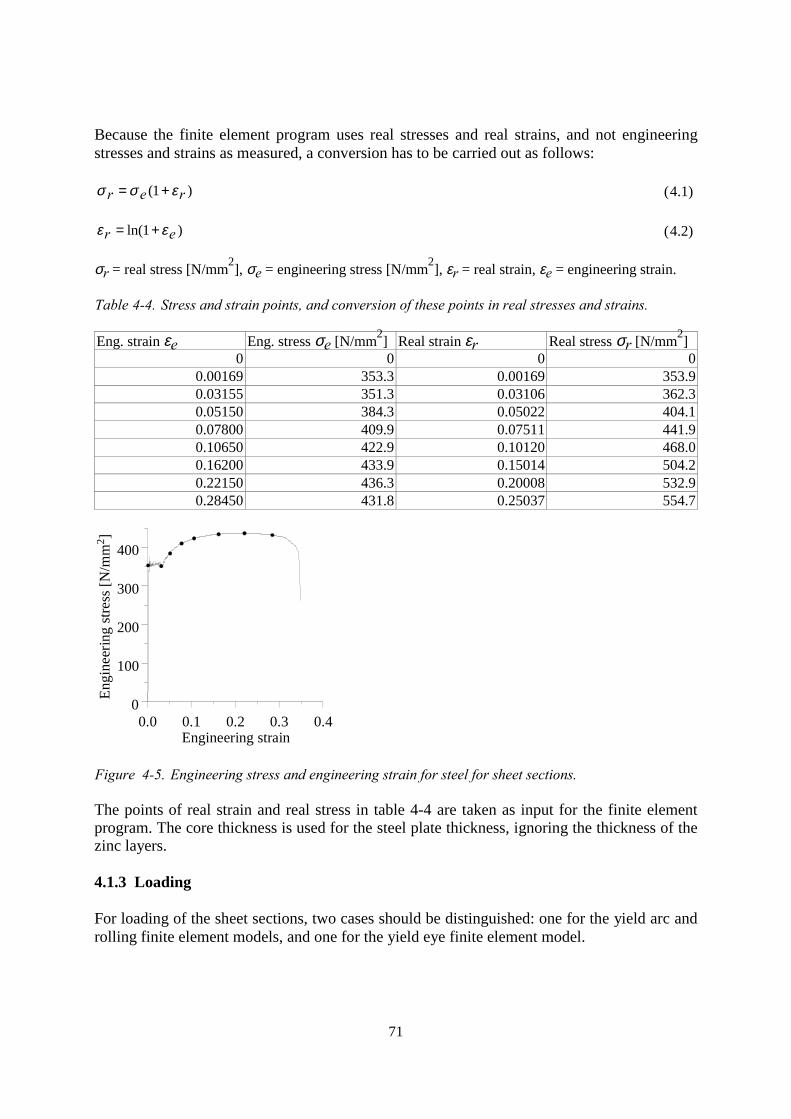
71
Because the finite element program uses real stresses and real strains, and not engineeringstresses and strains as measured, a conversion has to be carried out as follows:
)1( rer εσσ += (4.1)
)1ln( er εε += (4.2)
σr = real stress [N/mm2], σe = engineering stress [N/mm2], εr = real strain, εe = engineering strain.
Table 4-4. Stress and strain points, and conversion of these points in real stresses and strains.
Eng. strain εe Eng. stress σe [N/mm2] Real strain εr Real stress σr [N/mm2]0 0 0 0
0.00169 353.3 0.00169 353.90.03155 351.3 0.03106 362.30.05150 384.3 0.05022 404.10.07800 409.9 0.07511 441.90.10650 422.9 0.10120 468.00.16200 433.9 0.15014 504.20.22150 436.3 0.20008 532.90.28450 431.8 0.25037 554.7
0.0 0.1 0.2 0.3 0.4Engineering strain
0
100
200
300
400
Engi
neer
ing
stre
ss [N
/mm
2 ]
Figure 4-5. Engineering stress and engineering strain for steel for sheet sections.
The points of real strain and real stress in table 4-4 are taken as input for the finite elementprogram. The core thickness is used for the steel plate thickness, ignoring the thickness of thezinc layers.
4.1.3 Loading
For loading of the sheet sections, two cases should be distinguished: one for the yield arc androlling finite element models, and one for the yield eye finite element model.
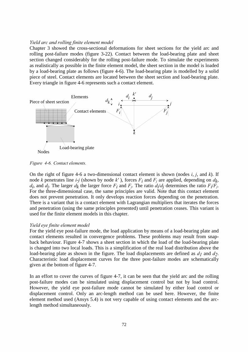
72
Yield arc and rolling finite element modelChapter 3 showed the cross-sectional deformations for sheet sections for the yield arc androlling post-failure modes (figure 3-22). Contact between the load-bearing plate and sheetsection changed considerably for the rolling post-failure mode. To simulate the experimentsas realistically as possible in the finite element model, the sheet section in the model is loadedby a load-bearing plate as follows (figure 4-6). The load-bearing plate is modelled by a solidpiece of steel. Contact elements are located between the sheet section and load-bearing plate.Every triangle in figure 4-6 represents such a contact element.
Load-bearing plate
Piece of sheet section
Nodes
Elements
Contact elementsi j
k
k'di djdk
Fi Fj
Figure 4-6. Contact elements.
On the right of figure 4-6 a two-dimensional contact element is shown (nodes i, j, and k). Ifnode k penetrates line i-j (shown by node k' ), forces Fi and Fj are applied, depending on dk,di, and dj. The larger dk the larger force Fi and Fj. The ratio di/dj determines the ratio Fi/Fj.For the three-dimensional case, the same principles are valid. Note that this contact elementdoes not prevent penetration. It only develops reaction forces depending on the penetration.There is a variant that is a contact element with Lagrangian multipliers that iterates the forcesand penetration (using the same principles presented) until penetration ceases. This variant isused for the finite element models in this chapter.
Yield eye finite element modelFor the yield eye post-failure mode, the load application by means of a load-bearing plate andcontact elements resulted in convergence problems. These problems may result from snap-back behaviour. Figure 4-7 shows a sheet section in which the load of the load-bearing plateis changed into two local loads. This is a simplification of the real load distribution above theload-bearing plate as shown in the figure. The load displacements are defined as d1 and d2.Characteristic load displacement curves for the three post-failure modes are schematicallygiven at the bottom of figure 4-7.
In an effort to cover the curves of figure 4-7, it can be seen that the yield arc and the rollingpost-failure modes can be simulated using displacement control but not by load control.However, the yield eye post-failure mode cannot be simulated by either load control ordisplacement control. Only an arc-length method can be used here. However, the finiteelement method used (Ansys 5.4) is not very capable of using contact elements and the arc-length method simultaneously.
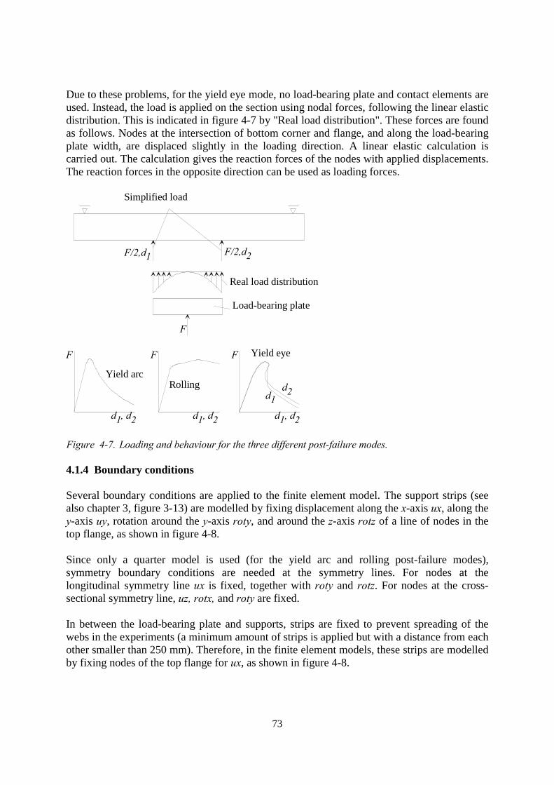
73
Due to these problems, for the yield eye mode, no load-bearing plate and contact elements areused. Instead, the load is applied on the section using nodal forces, following the linear elasticdistribution. This is indicated in figure 4-7 by "Real load distribution". These forces are foundas follows. Nodes at the intersection of bottom corner and flange, and along the load-bearingplate width, are displaced slightly in the loading direction. A linear elastic calculation iscarried out. The calculation gives the reaction forces of the nodes with applied displacements.The reaction forces in the opposite direction can be used as loading forces.
F/2,d1
F
F/2,d2
Load-bearing plate
Simplified load
Real load distribution
d1, d2d1, d2 d1, d2
FF F
RollingYield arc
Yield eye
d1d2
Figure 4-7. Loading and behaviour for the three different post-failure modes.
4.1.4 Boundary conditions
Several boundary conditions are applied to the finite element model. The support strips (seealso chapter 3, figure 3-13) are modelled by fixing displacement along the x-axis ux, along they-axis uy, rotation around the y-axis roty, and around the z-axis rotz of a line of nodes in thetop flange, as shown in figure 4-8.
Since only a quarter model is used (for the yield arc and rolling post-failure modes),symmetry boundary conditions are needed at the symmetry lines. For nodes at thelongitudinal symmetry line ux is fixed, together with roty and rotz. For nodes at the cross-sectional symmetry line, uz, rotx, and roty are fixed.
In between the load-bearing plate and supports, strips are fixed to prevent spreading of thewebs in the experiments (a minimum amount of strips is applied but with a distance from eachother smaller than 250 mm). Therefore, in the finite element models, these strips are modelledby fixing nodes of the top flange for ux, as shown in figure 4-8.
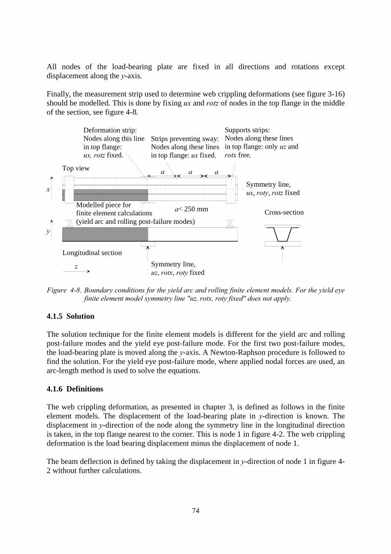
74
All nodes of the load-bearing plate are fixed in all directions and rotations exceptdisplacement along the y-axis.
Finally, the measurement strip used to determine web crippling deformations (see figure 3-16)should be modelled. This is done by fixing ux and rotz of nodes in the top flange in the middleof the section, see figure 4-8.
Longitudinal section
Top view
Cross-sectionModelled piece forfinite element calculations(yield arc and rolling post-failure modes)
Symmetry line, ux, roty, rotz fixed
Symmetry line,uz, rotx, roty fixed
Strips preventing sway:Nodes along these linesin top flange: ux fixed.
a< 250 mm
Deformation strip:Nodes along this linein top flange:ux, rotz fixed.
z
x
y
Supports strips:Nodes along these linesin top flange: only uz androtx free.
a a a
Figure 4-8. Boundary conditions for the yield arc and rolling finite element models. For the yield eyefinite element model symmetry line "uz, rotx, roty fixed" does not apply.
4.1.5 Solution
The solution technique for the finite element models is different for the yield arc and rollingpost-failure modes and the yield eye post-failure mode. For the first two post-failure modes,the load-bearing plate is moved along the y-axis. A Newton-Raphson procedure is followed tofind the solution. For the yield eye post-failure mode, where applied nodal forces are used, anarc-length method is used to solve the equations.
4.1.6 Definitions
The web crippling deformation, as presented in chapter 3, is defined as follows in the finiteelement models. The displacement of the load-bearing plate in y-direction is known. Thedisplacement in y-direction of the node along the symmetry line in the longitudinal directionis taken, in the top flange nearest to the corner. This is node 1 in figure 4-2. The web cripplingdeformation is the load bearing displacement minus the displacement of node 1.
The beam deflection is defined by taking the displacement in y-direction of node 1 in figure 4-2 without further calculations.

75
The support rotation is defined as the rotation around the x-axis of a node at the support. Thisnode is at the same location of node 1 in figure 4-2, except in the longitudinal direction. Inthat direction, it is not at the symmetry line, but at the support.
These three items are defined to make a good comparison possible between the experimentsand the finite element model.
4.1.7 Overview finite element models
Table 4-5 gives an overview of the three finite element models and their differences.
Table 4-5. Overview finite element models.
Rolling model Yield arc model Yield eye modelMesh and elements Quarter model. Half model.
Fine mesh for bottomcorner and web.
Fine mesh for web andbottom flange.
Fine mesh for bottomflange.
Loading Load-bearing plate and contact elements. Applied nodal forces.Solution Newton-Raphson. Arc-length.
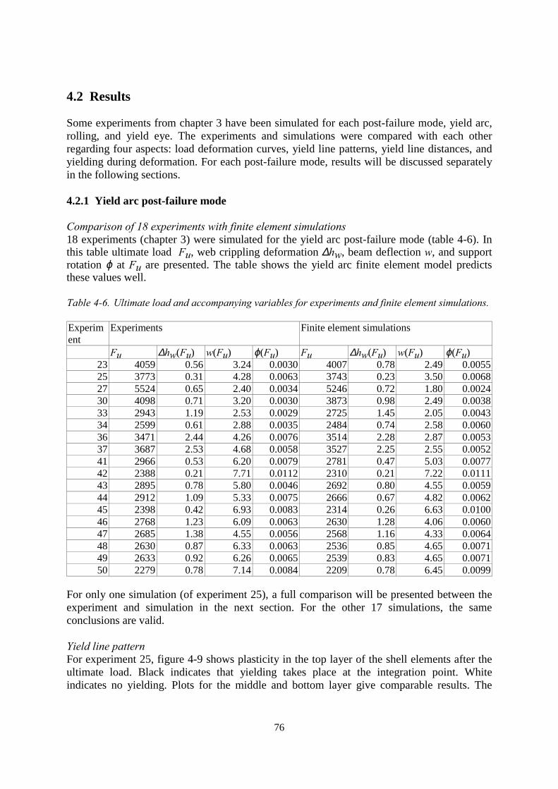
76
4.2 Results
Some experiments from chapter 3 have been simulated for each post-failure mode, yield arc,rolling, and yield eye. The experiments and simulations were compared with each otherregarding four aspects: load deformation curves, yield line patterns, yield line distances, andyielding during deformation. For each post-failure mode, results will be discussed separatelyin the following sections.
4.2.1 Yield arc post-failure mode
Comparison of 18 experiments with finite element simulations18 experiments (chapter 3) were simulated for the yield arc post-failure mode (table 4-6). Inthis table ultimate load Fu, web crippling deformation ∆hw, beam deflection w, and supportrotation ϕ at Fu are presented. The table shows the yield arc finite element model predictsthese values well.
Table 4-6. Ultimate load and accompanying variables for experiments and finite element simulations.
Experiment
Experiments Finite element simulations
Fu ∆hw(Fu) w(Fu) ϕ(Fu) Fu ∆hw(Fu) w(Fu) ϕ(Fu)23 4059 0.56 3.24 0.0030 4007 0.78 2.49 0.005525 3773 0.31 4.28 0.0063 3743 0.23 3.50 0.006827 5524 0.65 2.40 0.0034 5246 0.72 1.80 0.002430 4098 0.71 3.20 0.0030 3873 0.98 2.49 0.003833 2943 1.19 2.53 0.0029 2725 1.45 2.05 0.004334 2599 0.61 2.88 0.0035 2484 0.74 2.58 0.006036 3471 2.44 4.26 0.0076 3514 2.28 2.87 0.005337 3687 2.53 4.68 0.0058 3527 2.25 2.55 0.005241 2966 0.53 6.20 0.0079 2781 0.47 5.03 0.007742 2388 0.21 7.71 0.0112 2310 0.21 7.22 0.011143 2895 0.78 5.80 0.0046 2692 0.80 4.55 0.005944 2912 1.09 5.33 0.0075 2666 0.67 4.82 0.006245 2398 0.42 6.93 0.0083 2314 0.26 6.63 0.010046 2768 1.23 6.09 0.0063 2630 1.28 4.06 0.006047 2685 1.38 4.55 0.0056 2568 1.16 4.33 0.006448 2630 0.87 6.33 0.0063 2536 0.85 4.65 0.007149 2633 0.92 6.26 0.0065 2539 0.83 4.65 0.007150 2279 0.78 7.14 0.0084 2209 0.78 6.45 0.0099
For only one simulation (of experiment 25), a full comparison will be presented between theexperiment and simulation in the next section. For the other 17 simulations, the sameconclusions are valid.
Yield line patternFor experiment 25, figure 4-9 shows plasticity in the top layer of the shell elements after theultimate load. Black indicates that yielding takes place at the integration point. Whiteindicates no yielding. Plots for the middle and bottom layer give comparable results. The
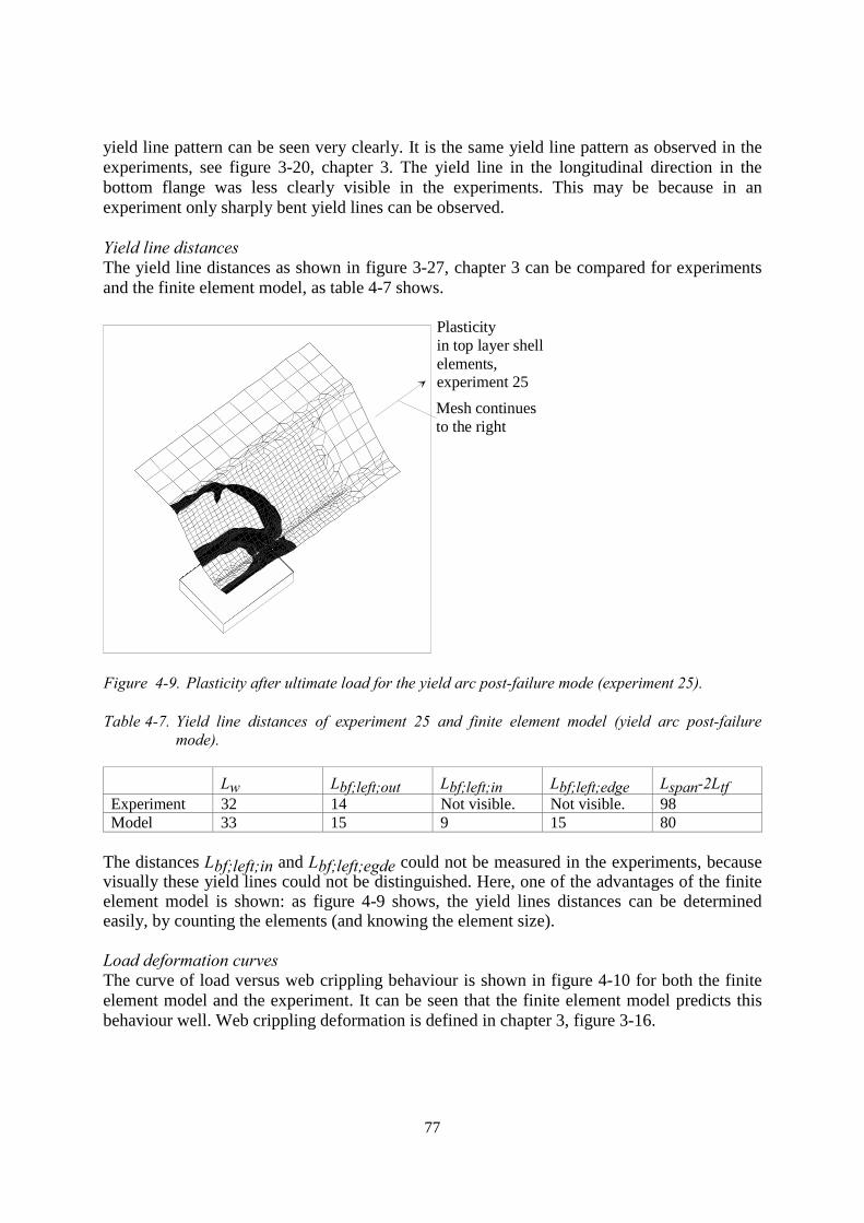
77
yield line pattern can be seen very clearly. It is the same yield line pattern as observed in theexperiments, see figure 3-20, chapter 3. The yield line in the longitudinal direction in thebottom flange was less clearly visible in the experiments. This may be because in anexperiment only sharply bent yield lines can be observed.
Yield line distancesThe yield line distances as shown in figure 3-27, chapter 3 can be compared for experimentsand the finite element model, as table 4-7 shows.
Plasticityin top layer shellelements,experiment 25Mesh continuesto the right
Figure 4-9. Plasticity after ultimate load for the yield arc post-failure mode (experiment 25).
Table 4-7. Yield line distances of experiment 25 and finite element model (yield arc post-failuremode).
Lw Lbf;left;out Lbf;left;in Lbf;left;edge Lspan-2LtfExperiment 32 14 Not visible. Not visible. 98Model 33 15 9 15 80
The distances Lbf;left;in and Lbf;left;egde could not be measured in the experiments, becausevisually these yield lines could not be distinguished. Here, one of the advantages of the finiteelement model is shown: as figure 4-9 shows, the yield lines distances can be determinedeasily, by counting the elements (and knowing the element size).
Load deformation curvesThe curve of load versus web crippling behaviour is shown in figure 4-10 for both the finiteelement model and the experiment. It can be seen that the finite element model predicts thisbehaviour well. Web crippling deformation is defined in chapter 3, figure 3-16.
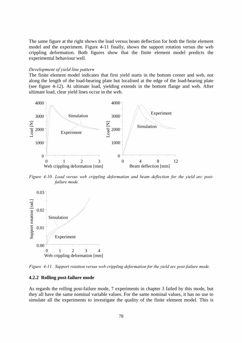
78
The same figure at the right shows the load versus beam deflection for both the finite elementmodel and the experiment. Figure 4-11 finally, shows the support rotation versus the webcrippling deformation. Both figures show that the finite element model predicts theexperimental behaviour well.
Development of yield line patternThe finite element model indicates that first yield starts in the bottom corner and web, notalong the length of the load-bearing plate but localised at the edge of the load-bearing plate(see figure 4-12). At ultimate load, yielding extends in the bottom flange and web. Afterultimate load, clear yield lines occur in the web.
0 1 2 3Web crippling deformation [mm]
0
1000
2000
3000
4000
Load
[N]
Simulation
Experiment
0 4 8 12Beam deflection [mm]
0
1000
2000
3000
4000
Experiment
Simulation
Load
[N]
Figure 4-10. Load versus web crippling deformation and beam deflection for the yield arc post-failure mode.
Supp
ort r
otat
ion
[rad
.]
0 1 2 3 4Web crippling deformation [mm]
0.00
0.01
0.02
0.03
Experiment
Simulation
Figure 4-11. Support rotation versus web crippling deformation for the yield arc post-failure mode.
4.2.2 Rolling post-failure mode
As regards the rolling post-failure mode, 7 experiments in chapter 3 failed by this mode, butthey all have the same nominal variable values. For the same nominal values, it has no use tosimulate all the experiments to investigate the quality of the finite element model. This is
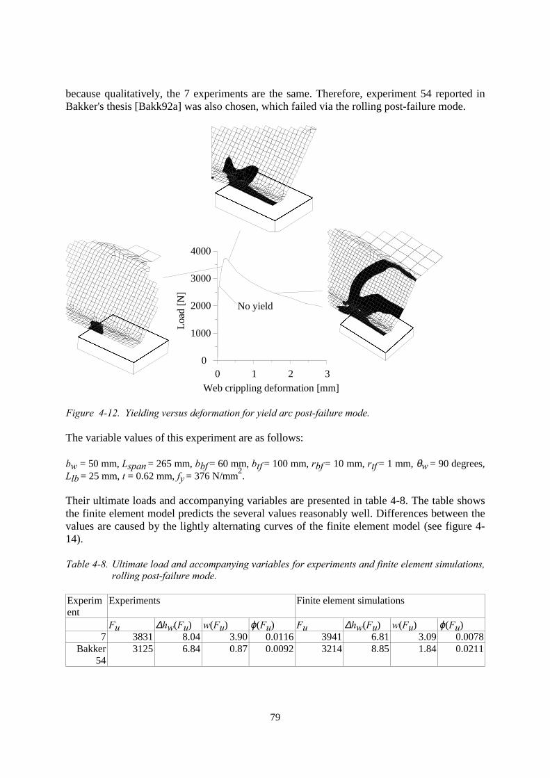
79
because qualitatively, the 7 experiments are the same. Therefore, experiment 54 reported inBakker's thesis [Bakk92a] was also chosen, which failed via the rolling post-failure mode.
0 1 2 3Web crippling deformation [mm]
0
1000
2000
3000
4000
Load
[N]
No yield
Figure 4-12. Yielding versus deformation for yield arc post-failure mode.
The variable values of this experiment are as follows:
bw = 50 mm, Lspan = 265 mm, bbf = 60 mm, btf = 100 mm, rbf = 10 mm, rtf = 1 mm, θw = 90 degrees,Llb = 25 mm, t = 0.62 mm, fy = 376 N/mm2.
Their ultimate loads and accompanying variables are presented in table 4-8. The table showsthe finite element model predicts the several values reasonably well. Differences between thevalues are caused by the lightly alternating curves of the finite element model (see figure 4-14).
Table 4-8. Ultimate load and accompanying variables for experiments and finite element simulations,rolling post-failure mode.
Experiment
Experiments Finite element simulations
Fu ∆hw(Fu) w(Fu) ϕ(Fu) Fu ∆hw(Fu) w(Fu) ϕ(Fu)7 3831 8.04 3.90 0.0116 3941 6.81 3.09 0.0078
Bakker54
3125 6.84 0.87 0.0092 3214 8.85 1.84 0.0211
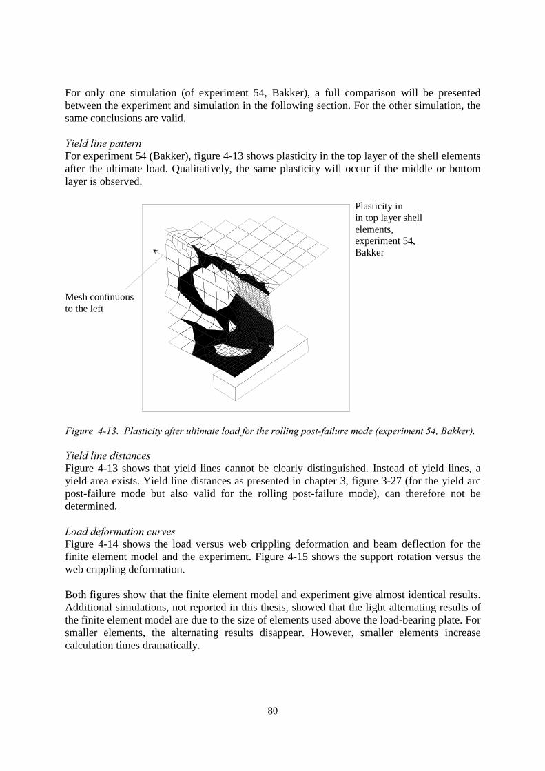
80
For only one simulation (of experiment 54, Bakker), a full comparison will be presentedbetween the experiment and simulation in the following section. For the other simulation, thesame conclusions are valid.
Yield line patternFor experiment 54 (Bakker), figure 4-13 shows plasticity in the top layer of the shell elementsafter the ultimate load. Qualitatively, the same plasticity will occur if the middle or bottomlayer is observed.
Plasticity inin top layer shellelements,experiment 54, Bakker
Mesh continuousto the left
Figure 4-13. Plasticity after ultimate load for the rolling post-failure mode (experiment 54, Bakker).
Yield line distancesFigure 4-13 shows that yield lines cannot be clearly distinguished. Instead of yield lines, ayield area exists. Yield line distances as presented in chapter 3, figure 3-27 (for the yield arcpost-failure mode but also valid for the rolling post-failure mode), can therefore not bedetermined.
Load deformation curvesFigure 4-14 shows the load versus web crippling deformation and beam deflection for thefinite element model and the experiment. Figure 4-15 shows the support rotation versus theweb crippling deformation.
Both figures show that the finite element model and experiment give almost identical results.Additional simulations, not reported in this thesis, showed that the light alternating results ofthe finite element model are due to the size of elements used above the load-bearing plate. Forsmaller elements, the alternating results disappear. However, smaller elements increasecalculation times dramatically.
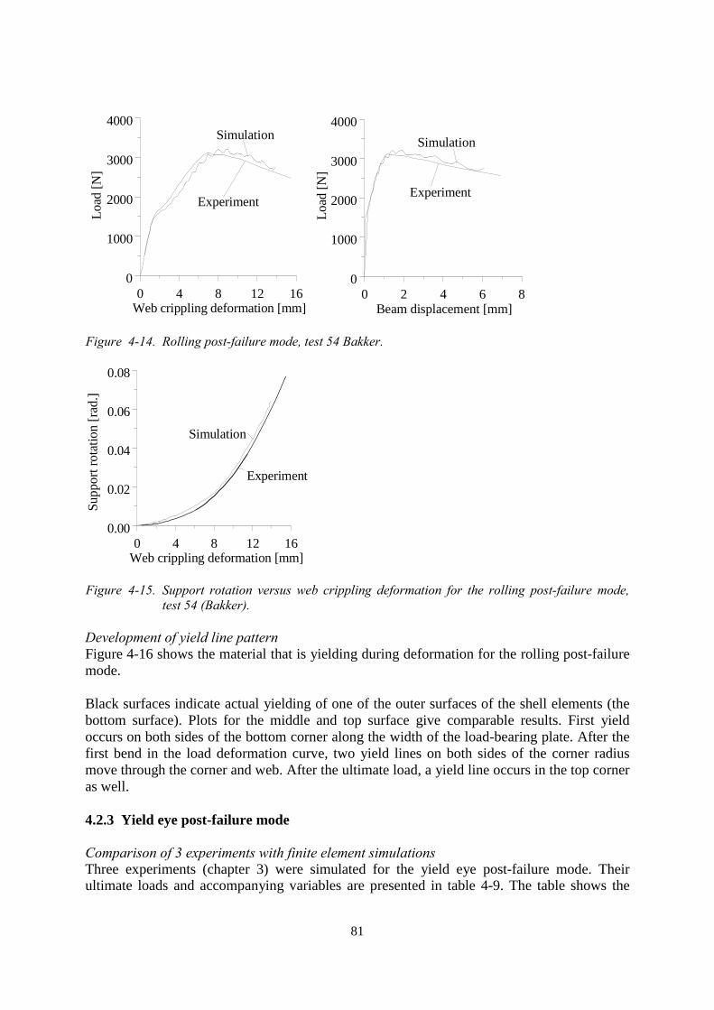
81
Load
[N]
0 4 8 12 16Web crippling deformation [mm]
0
1000
2000
3000
4000
Experiment
Simulation
0 2 4 6 8Beam displacement [mm]
0
1000
2000
3000
4000Simulation
Experiment
Load
[N]
Figure 4-14. Rolling post-failure mode, test 54 Bakker.
Supp
ort r
otat
ion
[rad
.]
0 4 8 12 16Web crippling deformation [mm]
0.00
0.02
0.04
0.06
0.08
Simulation
Experiment
Figure 4-15. Support rotation versus web crippling deformation for the rolling post-failure mode,test 54 (Bakker).
Development of yield line patternFigure 4-16 shows the material that is yielding during deformation for the rolling post-failuremode.
Black surfaces indicate actual yielding of one of the outer surfaces of the shell elements (thebottom surface). Plots for the middle and top surface give comparable results. First yieldoccurs on both sides of the bottom corner along the width of the load-bearing plate. After thefirst bend in the load deformation curve, two yield lines on both sides of the corner radiusmove through the corner and web. After the ultimate load, a yield line occurs in the top corneras well.
4.2.3 Yield eye post-failure mode
Comparison of 3 experiments with finite element simulationsThree experiments (chapter 3) were simulated for the yield eye post-failure mode. Theirultimate loads and accompanying variables are presented in table 4-9. The table shows the
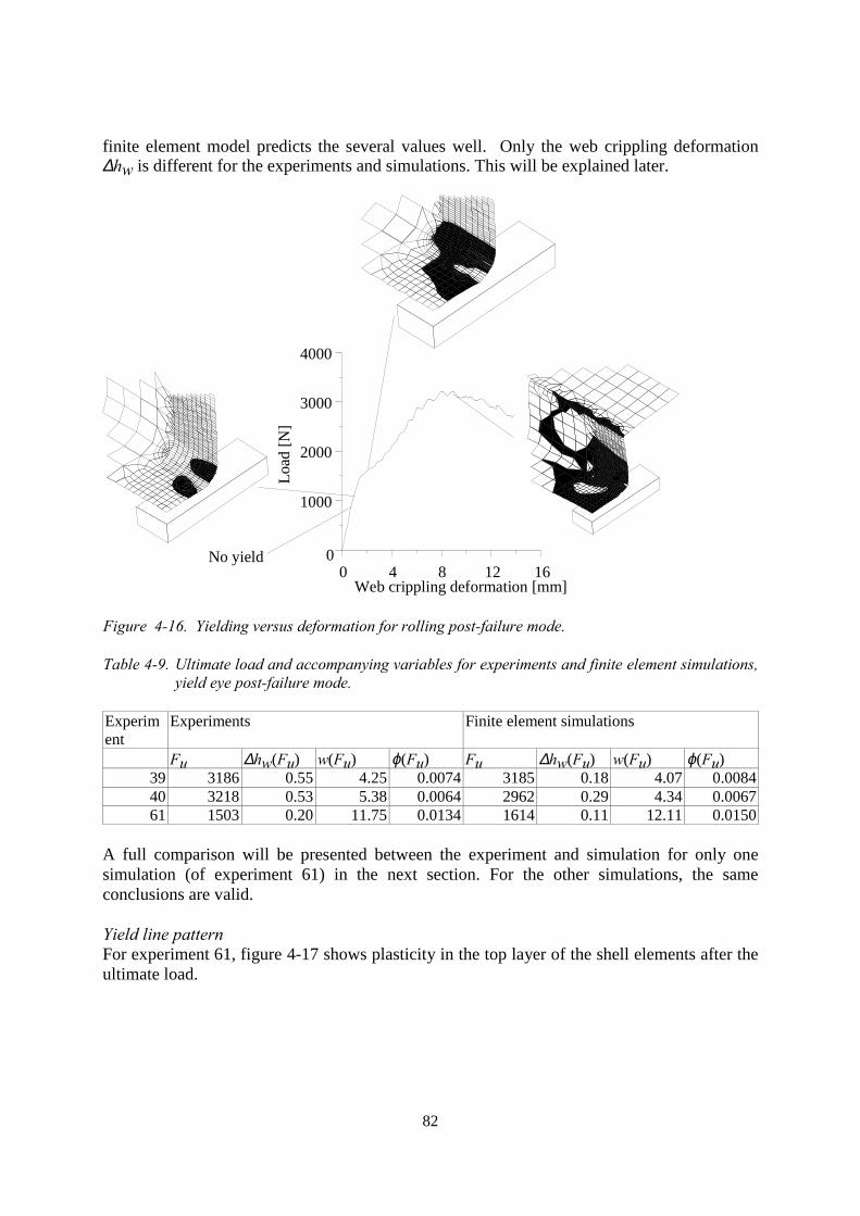
82
finite element model predicts the several values well. Only the web crippling deformation∆hw is different for the experiments and simulations. This will be explained later.
0 4 8 12 16Web crippling deformation [mm]
0
1000
2000
3000
4000
Load
[N]
No yield
Figure 4-16. Yielding versus deformation for rolling post-failure mode.
Table 4-9. Ultimate load and accompanying variables for experiments and finite element simulations,yield eye post-failure mode.
Experiment
Experiments Finite element simulations
Fu ∆hw(Fu) w(Fu) ϕ(Fu) Fu ∆hw(Fu) w(Fu) ϕ(Fu)39 3186 0.55 4.25 0.0074 3185 0.18 4.07 0.008440 3218 0.53 5.38 0.0064 2962 0.29 4.34 0.006761 1503 0.20 11.75 0.0134 1614 0.11 12.11 0.0150
A full comparison will be presented between the experiment and simulation for only onesimulation (of experiment 61) in the next section. For the other simulations, the sameconclusions are valid.
Yield line patternFor experiment 61, figure 4-17 shows plasticity in the top layer of the shell elements after theultimate load.
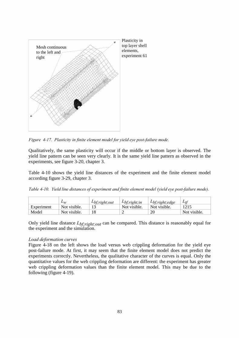
83
Plasticity intop layer shellelements,experiment 61
Mesh continuousto the left andright
Figure 4-17. Plasticity in finite element model for yield eye post-failure mode.
Qualitatively, the same plasticity will occur if the middle or bottom layer is observed. Theyield line pattern can be seen very clearly. It is the same yield line pattern as observed in theexperiments, see figure 3-20, chapter 3.
Table 4-10 shows the yield line distances of the experiment and the finite element modelaccording figure 3-29, chapter 3.
Table 4-10. Yield line distances of experiment and finite element model (yield eye post-failure mode).
Lw Lbf;right;out Lbf;right;in Lbf;right;edge LtfExperiment Not visible. 13 Not visible. Not visible. 1215Model Not visible. 18 2 20 Not visible.
Only yield line distance Lbf;right;out can be compared. This distance is reasonably equal forthe experiment and the simulation.
Load deformation curvesFigure 4-18 on the left shows the load versus web crippling deformation for the yield eyepost-failure mode. At first, it may seem that the finite element model does not predict theexperiments correctly. Nevertheless, the qualitative character of the curves is equal. Only thequantitative values for the web crippling deformation are different: the experiment has greaterweb crippling deformation values than the finite element model. This may be due to thefollowing (figure 4-19).
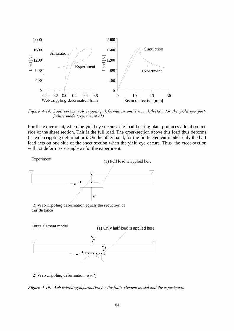
84
-0.4 -0.2 0.0 0.2 0.4 0.6Web crippling deformation [mm]
0
400
800
1200
1600
2000
Load
[N]
Experiment
Simulation
0 10 20 30Beam deflection [mm]
0
400
800
1200
1600
2000
Simulation
ExperimentLoad
[N]
Figure 4-18. Load versus web crippling deformation and beam deflection for the yield eye post-failure mode (experiment 61).
For the experiment, when the yield eye occurs, the load-bearing plate produces a load on oneside of the sheet section. This is the full load. The cross-section above this load thus deforms(as web crippling deformation). On the other hand, for the finite element model, only the halfload acts on one side of the sheet section when the yield eye occurs. Thus, the cross-sectionwill not deform as strongly as for the experiment.
F
d1
d2
(2) Web crippling deformation: d1-d2
(2) Web crippling deformation equals the reduction of this distance
Experiment (1) Full load is applied here
Finite element model (1) Only half load is applied here
Figure 4-19. Web crippling deformation for the finite element model and the experiment.
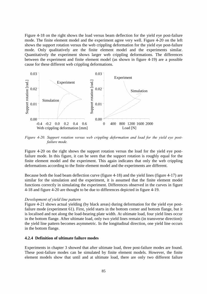
85
Figure 4-18 on the right shows the load versus beam deflection for the yield eye post-failuremode. The finite element model and the experiment agree very well. Figure 4-20 on the leftshows the support rotation versus the web crippling deformation for the yield eye post-failuremode. Only qualitatively are the finite element model and the experiments similar.Quantitatively the experiment shows larger web crippling deformations. The differencesbetween the experiment and finite element model (as shown in figure 4-19) are a possiblecause for these different web crippling deformations.
-0.4 -0.2 0.0 0.2 0.4 0.6Web crippling deformation [mm]
0.00
0.01
0.02
0.03
Supp
ort r
otat
ion
[rad
.]
Simulation
Experiment
0 400 800 1200 1600 2000Load [N]
0.00
0.01
0.02
0.03Experiment
SimulationSu
ppor
t rot
atio
n [r
ad.]
Figure 4-20. Support rotation versus web crippling deformation and load for the yield eye post-failure mode.
Figure 4-20 on the right shows the support rotation versus the load for the yield eye post-failure mode. In this figure, it can be seen that the support rotation is roughly equal for thefinite element model and the experiment. This again indicates that only the web cripplingdeformations according to the finite element model and the experiments are different.
Because both the load beam deflection curve (figure 4-18) and the yield lines (figure 4-17) aresimilar for the simulation and the experiment, it is assumed that the finite element modelfunctions correctly in simulating the experiment. Differences observed in the curves in figure4-18 and figure 4-20 are thought to be due to differences depicted in figure 4-19.
Development of yield line patternFigure 4-21 shows actual yielding (by black areas) during deformation for the yield eye post-failure mode (experiment 61). First, yield starts in the bottom corner and bottom flange, but itis localised and not along the load-bearing plate width. At ultimate load, four yield lines occurin the bottom flange. After ultimate load, only two yield lines remain (in transverse direction):the yield line pattern becomes asymmetric. In the longitudinal direction, one yield line occursin the bottom flange.
4.2.4 Definition of ultimate failure modes
Experiments in chapter 3 showed that after ultimate load, three post-failure modes are found.These post-failure modes can be simulated by finite element models. However, the finiteelement models show that until and at ultimate load, there are only two different failure
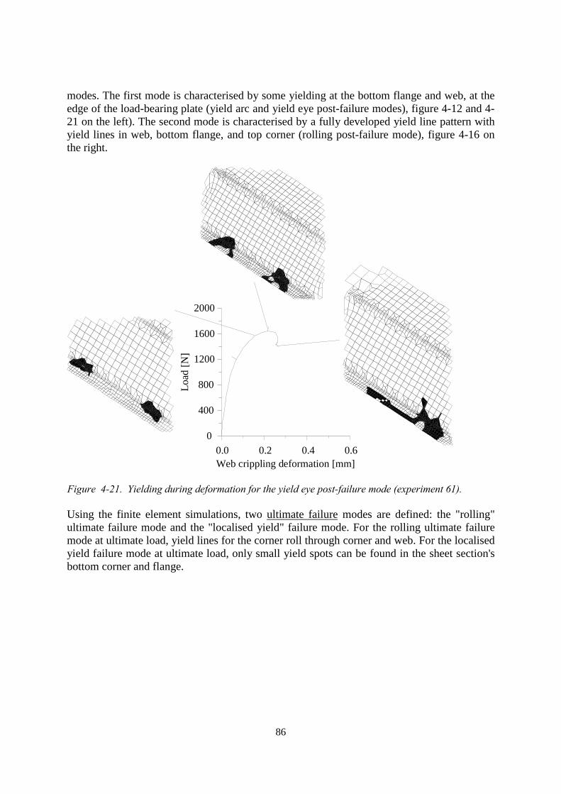
86
modes. The first mode is characterised by some yielding at the bottom flange and web, at theedge of the load-bearing plate (yield arc and yield eye post-failure modes), figure 4-12 and 4-21 on the left). The second mode is characterised by a fully developed yield line pattern withyield lines in web, bottom flange, and top corner (rolling post-failure mode), figure 4-16 onthe right.
0.0 0.2 0.4 0.6Web crippling deformation [mm]
0
400
800
1200
1600
2000
Load
[N]
Figure 4-21. Yielding during deformation for the yield eye post-failure mode (experiment 61).
Using the finite element simulations, two ultimate failure modes are defined: the "rolling"ultimate failure mode and the "localised yield" failure mode. For the rolling ultimate failuremode at ultimate load, yield lines for the corner roll through corner and web. For the localisedyield failure mode at ultimate load, only small yield spots can be found in the sheet section'sbottom corner and flange.
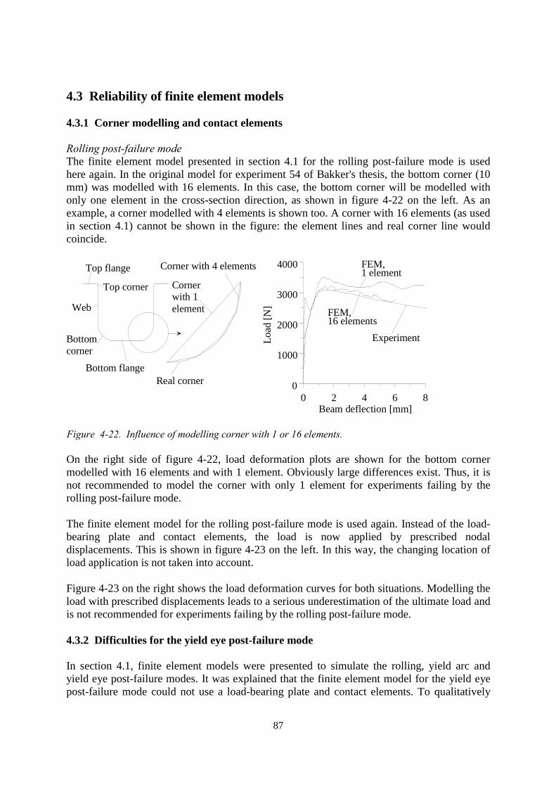
87
4.3 Reliability of finite element models
4.3.1 Corner modelling and contact elements
Rolling post-failure modeThe finite element model presented in section 4.1 for the rolling post-failure mode is usedhere again. In the original model for experiment 54 of Bakker's thesis, the bottom corner (10mm) was modelled with 16 elements. In this case, the bottom corner will be modelled withonly one element in the cross-section direction, as shown in figure 4-22 on the left. As anexample, a corner modelled with 4 elements is shown too. A corner with 16 elements (as usedin section 4.1) cannot be shown in the figure: the element lines and real corner line wouldcoincide.
Real corner
Corner with 4 elements
Cornerwith 1element
Top flange
Top corner
Web
Bottomcorner
Bottom flange
Experiment
FEM,16 elements
FEM,1 element
Load
[N]
0 2 4 6 8Beam deflection [mm]
0
1000
2000
3000
4000
Figure 4-22. Influence of modelling corner with 1 or 16 elements.
On the right side of figure 4-22, load deformation plots are shown for the bottom cornermodelled with 16 elements and with 1 element. Obviously large differences exist. Thus, it isnot recommended to model the corner with only 1 element for experiments failing by therolling post-failure mode.
The finite element model for the rolling post-failure mode is used again. Instead of the load-bearing plate and contact elements, the load is now applied by prescribed nodaldisplacements. This is shown in figure 4-23 on the left. In this way, the changing location ofload application is not taken into account.
Figure 4-23 on the right shows the load deformation curves for both situations. Modelling theload with prescribed displacements leads to a serious underestimation of the ultimate load andis not recommended for experiments failing by the rolling post-failure mode.
4.3.2 Difficulties for the yield eye post-failure mode
In section 4.1, finite element models were presented to simulate the rolling, yield arc andyield eye post-failure modes. It was explained that the finite element model for the yield eyepost-failure mode could not use a load-bearing plate and contact elements. To qualitatively
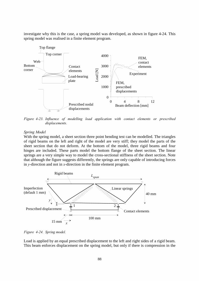
88
investigate why this is the case, a spring model was developed, as shown in figure 4-24. Thisspring model was realised in a finite element program.
Top flange
Top corner
WebBottomcorner
Load-bearingplate
Contactelements
Prescribed nodaldisplacements
0 4 8 12Beam deflection [mm]
0
1000
2000
3000
4000
Experiment
Load
[N]
FEM,prescribeddisplacements
FEM,contactelements
Figure 4-23. Influence of modelling load application with contact elements or prescribeddisplacements.
Spring ModelWith the spring model, a sheet section three point bending test can be modelled. The trianglesof rigid beams on the left and right of the model are very stiff; they model the parts of thesheet section that do not deform. At the bottom of the model, three rigid beams and fourhinges are included. These parts model the bottom flange of the sheet section. The linearsprings are a very simple way to model the cross-sectional stiffness of the sheet section. Notethat although the figure suggests differently, the springs are only capable of introducing forcesin y-direction and not in x-direction in the finite element program.
x
y
Lspan
40 mm
100 mm15 mm
Rigid beams
Linear springs
Contact elementsPrescribed displacement
Imperfection(default 1 mm)
1 2
Figure 4-24. Spring model.
Load is applied by an equal prescribed displacement to the left and right sides of a rigid beam.This beam enforces displacement on the spring model, but only if there is compression in the
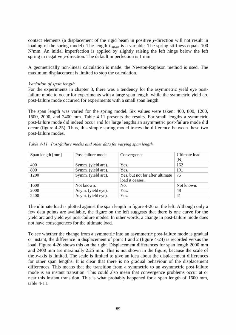
89
contact elements (a displacement of the rigid beam in positive y-direction will not result inloading of the spring model). The length Lspan is a variable. The spring stiffness equals 100N/mm. An initial imperfection is applied by slightly raising the left hinge below the leftspring in negative y-direction. The default imperfection is 1 mm.
A geometrically non-linear calculation is made: the Newton-Raphson method is used. Themaximum displacement is limited to stop the calculation.
Variation of span lengthFor the experiments in chapter 3, there was a tendency for the asymmetric yield eye post-failure mode to occur for experiments with a large span length, while the symmetric yield arcpost-failure mode occurred for experiments with a small span length.
The span length was varied for the spring model. Six values were taken: 400, 800, 1200,1600, 2000, and 2400 mm. Table 4-11 presents the results. For small lengths a symmetricpost-failure mode did indeed occur and for large lengths an asymmetric post-failure mode didoccur (figure 4-25). Thus, this simple spring model traces the difference between these twopost-failure modes.
Table 4-11. Post-failure modes and other data for varying span length.
Span length [mm] Post-failure mode Convergence Ultimate load[N]
400 Symm. (yield arc). Yes. 162800 Symm. (yield arc). Yes. 1011200 Symm. (yield arc). Yes, but not far after ultimate
load it ceases.75
1600 Not known. No. Not known.2000 Asym. (yield eye). Yes. 482400 Asym. (yield eye). Yes. 41
The ultimate load is plotted against the span length in figure 4-26 on the left. Although only afew data points are available, the figure on the left suggests that there is one curve for theyield arc and yield eye post-failure modes. In other words, a change in post-failure mode doesnot have consequences for the ultimate load.
To see whether the change from a symmetric into an asymmetric post-failure mode is gradualor instant, the difference in displacement of point 1 and 2 (figure 4-24) is recorded versus theload. Figure 4-26 shows this on the right. Displacement differences for span length 2000 mmand 2400 mm are maximally 2.25 mm. This is not shown in the figure, because the scale ofthe x-axis is limited. The scale is limited to give an idea about the displacement differencesfor other span lengths. It is clear that there is no gradual behaviour of the displacementdifferences. This means that the transition from a symmetric to an asymmetric post-failuremode is an instant transition. This could also mean that convergence problems occur at ornear this instant transition. This is what probably happened for a span length of 1600 mm,table 4-11.
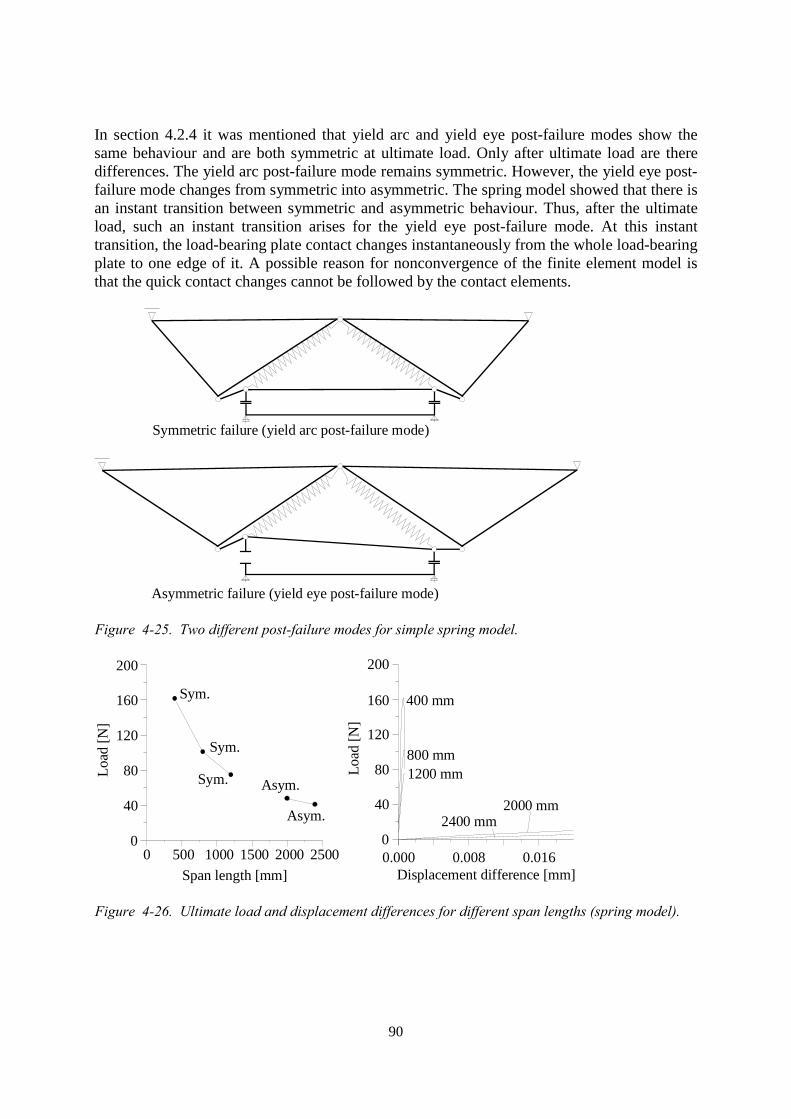
90
In section 4.2.4 it was mentioned that yield arc and yield eye post-failure modes show thesame behaviour and are both symmetric at ultimate load. Only after ultimate load are theredifferences. The yield arc post-failure mode remains symmetric. However, the yield eye post-failure mode changes from symmetric into asymmetric. The spring model showed that there isan instant transition between symmetric and asymmetric behaviour. Thus, after the ultimateload, such an instant transition arises for the yield eye post-failure mode. At this instanttransition, the load-bearing plate contact changes instantaneously from the whole load-bearingplate to one edge of it. A possible reason for nonconvergence of the finite element model isthat the quick contact changes cannot be followed by the contact elements.
Symmetric failure (yield arc post-failure mode)
Asymmetric failure (yield eye post-failure mode)
Figure 4-25. Two different post-failure modes for simple spring model.
0 500 1000 1500 2000 2500Span length [mm]
0
40
80
120
160
200
Sym.
Sym.
Sym. Asym.
Asym.
0.000 0.008 0.016Displacement difference [mm]
0
40
80
120
160
200
2400 mm2000 mm
1200 mm800 mm
400 mm
Load
[N]
Load
[N]
Figure 4-26. Ultimate load and displacement differences for different span lengths (spring model).
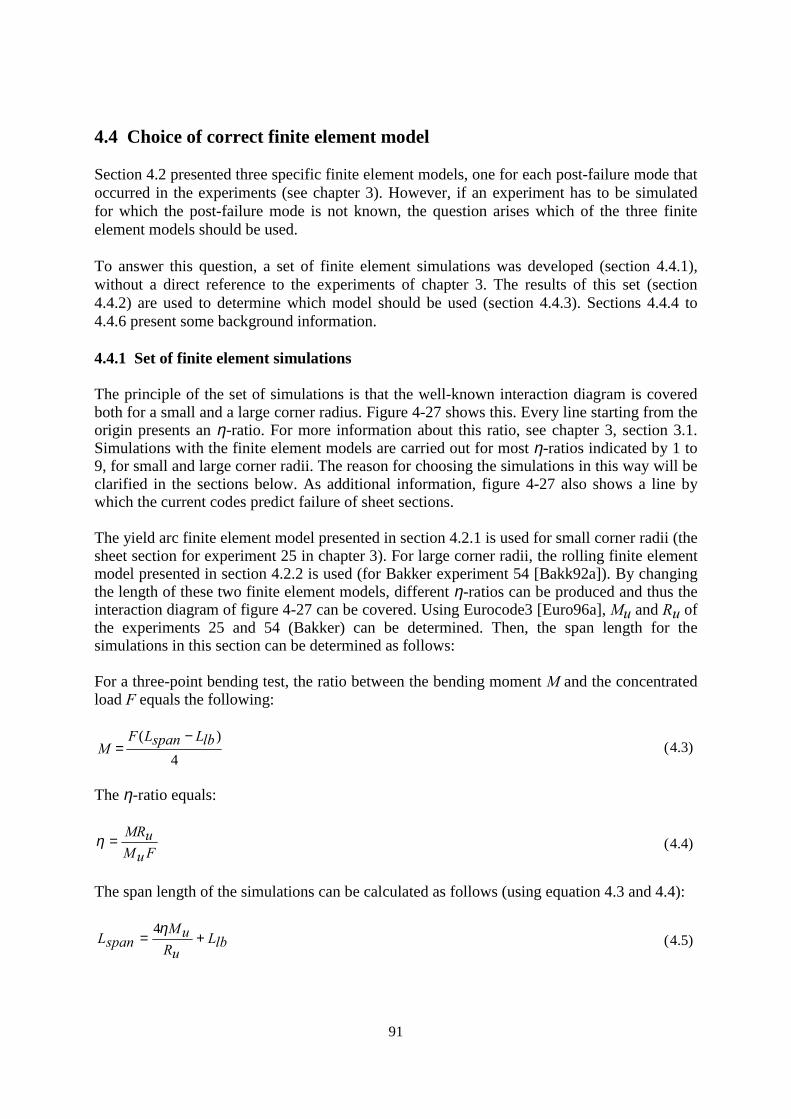
91
4.4 Choice of correct finite element model
Section 4.2 presented three specific finite element models, one for each post-failure mode thatoccurred in the experiments (see chapter 3). However, if an experiment has to be simulatedfor which the post-failure mode is not known, the question arises which of the three finiteelement models should be used.
To answer this question, a set of finite element simulations was developed (section 4.4.1),without a direct reference to the experiments of chapter 3. The results of this set (section4.4.2) are used to determine which model should be used (section 4.4.3). Sections 4.4.4 to4.4.6 present some background information.
4.4.1 Set of finite element simulations
The principle of the set of simulations is that the well-known interaction diagram is coveredboth for a small and a large corner radius. Figure 4-27 shows this. Every line starting from theorigin presents an η-ratio. For more information about this ratio, see chapter 3, section 3.1.Simulations with the finite element models are carried out for most η-ratios indicated by 1 to9, for small and large corner radii. The reason for choosing the simulations in this way will beclarified in the sections below. As additional information, figure 4-27 also shows a line bywhich the current codes predict failure of sheet sections.
The yield arc finite element model presented in section 4.2.1 is used for small corner radii (thesheet section for experiment 25 in chapter 3). For large corner radii, the rolling finite elementmodel presented in section 4.2.2 is used (for Bakker experiment 54 [Bakk92a]). By changingthe length of these two finite element models, different η-ratios can be produced and thus theinteraction diagram of figure 4-27 can be covered. Using Eurocode3 [Euro96a], Mu and Ru ofthe experiments 25 and 54 (Bakker) can be determined. Then, the span length for thesimulations in this section can be determined as follows:
For a three-point bending test, the ratio between the bending moment M and the concentratedload F equals the following:
4)( lbLspanLF
M−
= (4.3)
The η-ratio equals:
FuMuMR
=η (4.4)
The span length of the simulations can be calculated as follows (using equation 4.3 and 4.4):
lbLuR
uMspanL +=
η4(4.5)
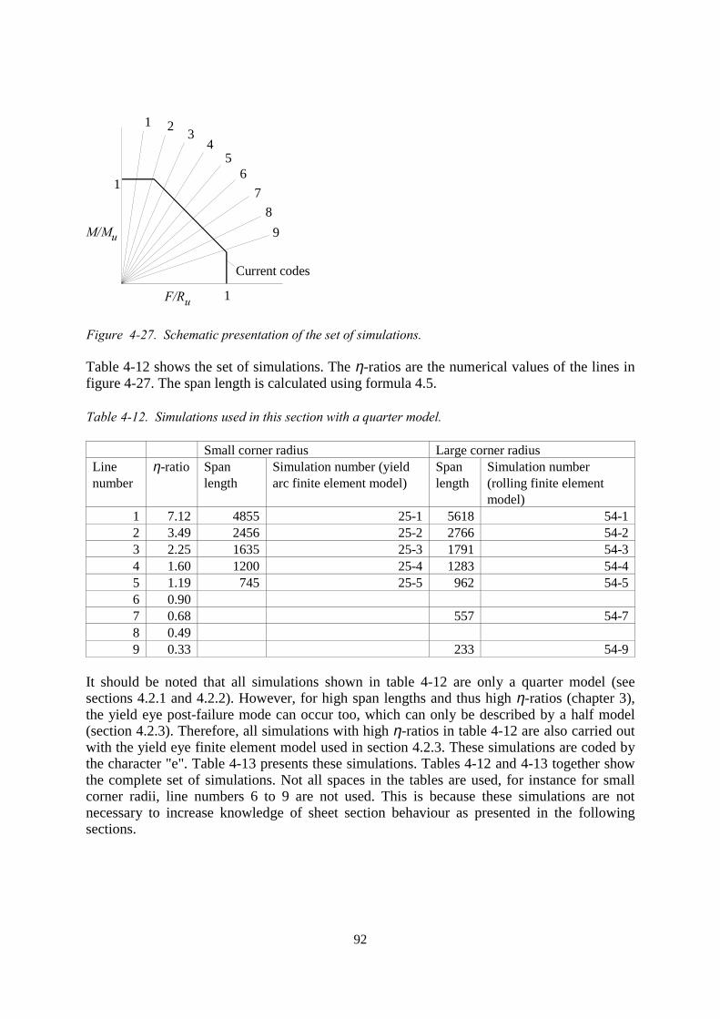
92
M/Mu
F/Ru 1
1
Current codes
1 2 34
56
78
9
Figure 4-27. Schematic presentation of the set of simulations.
Table 4-12 shows the set of simulations. The η-ratios are the numerical values of the lines infigure 4-27. The span length is calculated using formula 4.5.
Table 4-12. Simulations used in this section with a quarter model.
Small corner radius Large corner radiusLinenumber
η-ratio Spanlength
Simulation number (yieldarc finite element model)
Spanlength
Simulation number(rolling finite elementmodel)
1 7.12 4855 25-1 5618 54-12 3.49 2456 25-2 2766 54-23 2.25 1635 25-3 1791 54-34 1.60 1200 25-4 1283 54-45 1.19 745 25-5 962 54-56 0.907 0.68 557 54-78 0.499 0.33 233 54-9
It should be noted that all simulations shown in table 4-12 are only a quarter model (seesections 4.2.1 and 4.2.2). However, for high span lengths and thus high η-ratios (chapter 3),the yield eye post-failure mode can occur too, which can only be described by a half model(section 4.2.3). Therefore, all simulations with high η-ratios in table 4-12 are also carried outwith the yield eye finite element model used in section 4.2.3. These simulations are coded bythe character "e". Table 4-13 presents these simulations. Tables 4-12 and 4-13 together showthe complete set of simulations. Not all spaces in the tables are used, for instance for smallcorner radii, line numbers 6 to 9 are not used. This is because these simulations are notnecessary to increase knowledge of sheet section behaviour as presented in the followingsections.
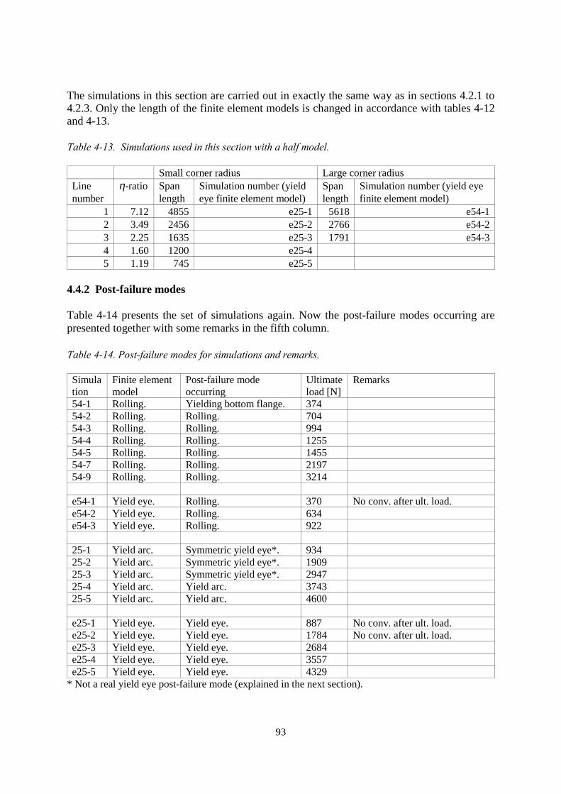
93
The simulations in this section are carried out in exactly the same way as in sections 4.2.1 to4.2.3. Only the length of the finite element models is changed in accordance with tables 4-12and 4-13.
Table 4-13. Simulations used in this section with a half model.
Small corner radius Large corner radiusLinenumber
η-ratio Spanlength
Simulation number (yieldeye finite element model)
Spanlength
Simulation number (yield eyefinite element model)
1 7.12 4855 e25-1 5618 e54-12 3.49 2456 e25-2 2766 e54-23 2.25 1635 e25-3 1791 e54-34 1.60 1200 e25-45 1.19 745 e25-5
4.4.2 Post-failure modes
Table 4-14 presents the set of simulations again. Now the post-failure modes occurring arepresented together with some remarks in the fifth column.
Table 4-14. Post-failure modes for simulations and remarks.
Simulation
Finite elementmodel
Post-failure modeoccurring
Ultimateload [N]
Remarks
54-1 Rolling. Yielding bottom flange. 37454-2 Rolling. Rolling. 70454-3 Rolling. Rolling. 99454-4 Rolling. Rolling. 125554-5 Rolling. Rolling. 145554-7 Rolling. Rolling. 219754-9 Rolling. Rolling. 3214
e54-1 Yield eye. Rolling. 370 No conv. after ult. load.e54-2 Yield eye. Rolling. 634e54-3 Yield eye. Rolling. 922
25-1 Yield arc. Symmetric yield eye*. 93425-2 Yield arc. Symmetric yield eye*. 190925-3 Yield arc. Symmetric yield eye*. 294725-4 Yield arc. Yield arc. 374325-5 Yield arc. Yield arc. 4600
e25-1 Yield eye. Yield eye. 887 No conv. after ult. load.e25-2 Yield eye. Yield eye. 1784 No conv. after ult. load.e25-3 Yield eye. Yield eye. 2684e25-4 Yield eye. Yield eye. 3557e25-5 Yield eye. Yield eye. 4329
* Not a real yield eye post-failure mode (explained in the next section).
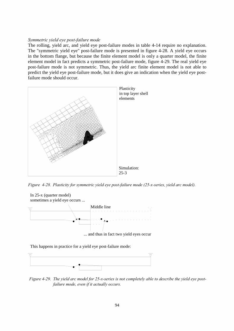
94
Symmetric yield eye post-failure modeThe rolling, yield arc, and yield eye post-failure modes in table 4-14 require no explanation.The "symmetric yield eye" post-failure mode is presented in figure 4-28. A yield eye occursin the bottom flange, but because the finite element model is only a quarter model, the finiteelement model in fact predicts a symmetric post-failure mode, figure 4-29. The real yield eyepost-failure mode is not symmetric. Thus, the yield arc finite element model is not able topredict the yield eye post-failure mode, but it does give an indication when the yield eye post-failure mode should occur.
Plasticityin top layer shellelements
Simulation:25-3
Figure 4-28. Plasticity for symmetric yield eye post-failure mode (25-x-series, yield arc model).
In 25-x (quarter model)sometimes a yield eye occurs ...
... and thus in fact two yield eyes occur
This happens in practice for a yield eye post-failure mode:
Middle line
Figure 4-29. The yield arc model for 25-x-series is not completely able to describe the yield eye post-failure mode, even if it actually occurs.
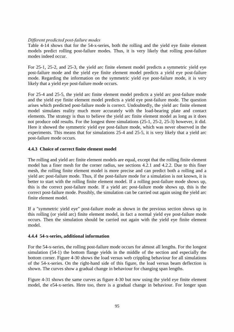
95
Different predicted post-failure modesTable 4-14 shows that for the 54-x-series, both the rolling and the yield eye finite elementmodels predict rolling post-failure modes. Thus, it is very likely that rolling post-failuremodes indeed occur.
For 25-1, 25-2, and 25-3, the yield arc finite element model predicts a symmetric yield eyepost-failure mode and the yield eye finite element model predicts a yield eye post-failuremode. Regarding the information on the symmetric yield eye post-failure mode, it is verylikely that a yield eye post-failure mode occurs.
For 25-4 and 25-5, the yield arc finite element model predicts a yield arc post-failure modeand the yield eye finite element model predicts a yield eye post-failure mode. The questionarises which predicted post-failure mode is correct. Undoubtedly, the yield arc finite elementmodel simulates reality much more accurately with the load-bearing plate and contactelements. The strategy is thus to believe the yield arc finite element model as long as it doesnot produce odd results. For the longest three simulations (25-1, 25-2, 25-3) however, it did.Here it showed the symmetric yield eye post-failure mode, which was never observed in theexperiments. This means that for simulations 25-4 and 25-5, it is very likely that a yield arcpost-failure mode occurs.
4.4.3 Choice of correct finite element model
The rolling and yield arc finite element models are equal, except that the rolling finite elementmodel has a finer mesh for the corner radius, see sections 4.2.1 and 4.2.2. Due to this finermesh, the rolling finite element model is more precise and can predict both a rolling and ayield arc post-failure mode. Thus, if the post-failure mode for a simulation is not known, it isbetter to start with the rolling finite element model. If a rolling post-failure mode shows up,this is the correct post-failure mode. If a yield arc post-failure mode shows up, this is thecorrect post-failure mode. Possibly, the simulation can be carried out again using the yield arcfinite element model.
If a "symmetric yield eye" post-failure mode as shown in the previous section shows up inthis rolling (or yield arc) finite element model, in fact a normal yield eye post-failure modeoccurs. Then the simulation should be carried out again with the yield eye finite elementmodel.
4.4.4 54-x-series, additional information
For the 54-x-series, the rolling post-failure mode occurs for almost all lengths. For the longestsimulation (54-1) the bottom flange yields in the middle of the section and especially thebottom corner. Figure 4-30 shows the load versus web crippling behaviour for all simulationsof the 54-x-series. On the right-hand side of this figure, the load versus beam deflection isshown. The curves show a gradual change in behaviour for changing span lengths.
Figure 4-31 shows the same curves as figure 4-30 but now using the yield eye finite elementmodel, the e54-x-series. Here too, there is a gradual change in behaviour. For longer span
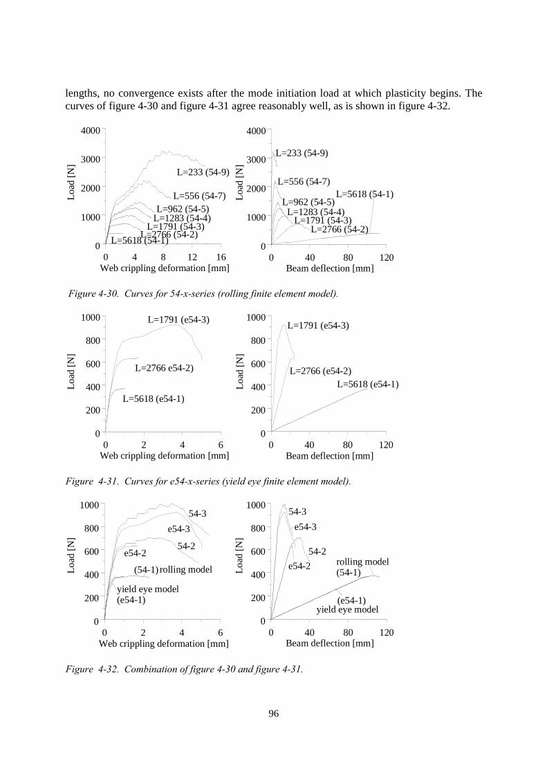
96
lengths, no convergence exists after the mode initiation load at which plasticity begins. Thecurves of figure 4-30 and figure 4-31 agree reasonably well, as is shown in figure 4-32.
0 40 80 120Beam deflection [mm]
0
1000
2000
3000
4000
L=5618 (54-1)
L=2766 (54-2)L=1791 (54-3)
L=1283 (54-4)L=962 (54-5)
L=556 (54-7)
L=233 (54-9)
Load
[N]
0 4 8 12 16Web crippling deformation [mm]
0
1000
2000
3000
4000
L=5618 (54-1)L=2766 (54-2)L=1791 (54-3)
L=1283 (54-4)L=962 (54-5)
L=556 (54-7)
L=233 (54-9)
Load
[N]
Figure 4-30. Curves for 54-x-series (rolling finite element model).
0 2 4 6Web crippling deformation [mm]
0
200
400
600
800
1000
L=5618 (e54-1)
L=2766 e54-2)
L=1791 (e54-3)
0 40 80 1200
200
400
600
800
1000
L=5618 (e54-1)L=2766 (e54-2)
L=1791 (e54-3)
Load
[N]
Load
[N]
Beam deflection [mm]
Figure 4-31. Curves for e54-x-series (yield eye finite element model).
0 2 4 6Web crippling deformation [mm]
0
200
400
600
800
1000
rolling model(54-1)
yield eye model(e54-1)
54-2e54-2
54-3e54-3
Load
[N]
0 40 80 120Beam deflection [mm]
0
200
400
600
800
1000
rolling model(54-1)
yield eye model(e54-1)
54-2e54-2
54-3e54-3
Load
[N]
Figure 4-32. Combination of figure 4-30 and figure 4-31.
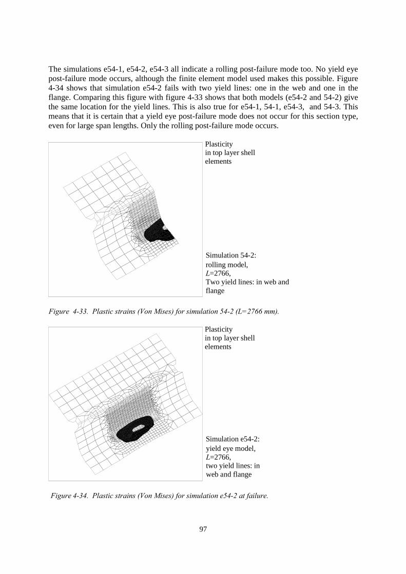
97
The simulations e54-1, e54-2, e54-3 all indicate a rolling post-failure mode too. No yield eyepost-failure mode occurs, although the finite element model used makes this possible. Figure4-34 shows that simulation e54-2 fails with two yield lines: one in the web and one in theflange. Comparing this figure with figure 4-33 shows that both models (e54-2 and 54-2) givethe same location for the yield lines. This is also true for e54-1, 54-1, e54-3, and 54-3. Thismeans that it is certain that a yield eye post-failure mode does not occur for this section type,even for large span lengths. Only the rolling post-failure mode occurs.
Plasticityin top layer shellelements
Simulation 54-2:rolling model,L=2766,Two yield lines: in web andflange
Figure 4-33. Plastic strains (Von Mises) for simulation 54-2 (L=2766 mm).
Plasticityin top layer shellelements
Simulation e54-2:yield eye model,L=2766,two yield lines: inweb and flange
Figure 4-34. Plastic strains (Von Mises) for simulation e54-2 at failure.
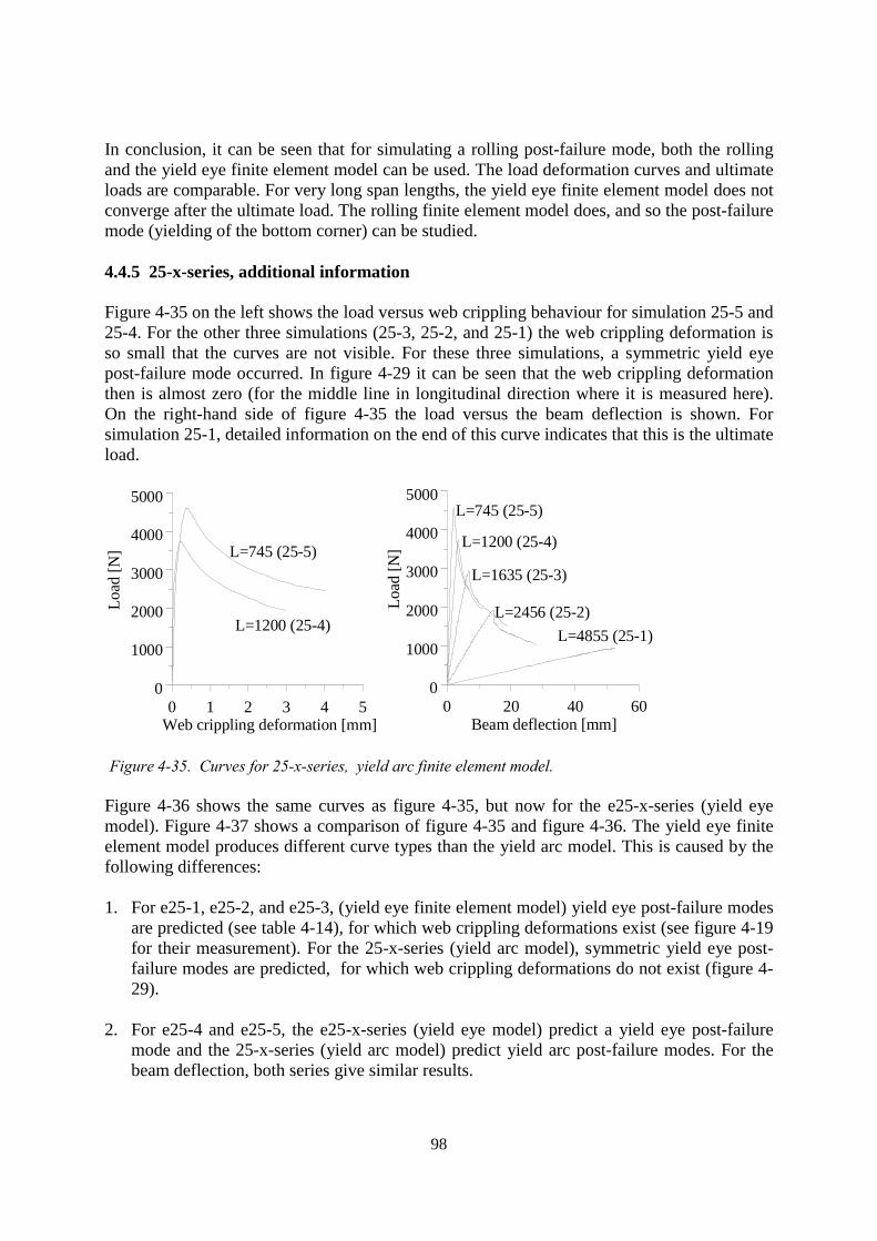
98
In conclusion, it can be seen that for simulating a rolling post-failure mode, both the rollingand the yield eye finite element model can be used. The load deformation curves and ultimateloads are comparable. For very long span lengths, the yield eye finite element model does notconverge after the ultimate load. The rolling finite element model does, and so the post-failuremode (yielding of the bottom corner) can be studied.
4.4.5 25-x-series, additional information
Figure 4-35 on the left shows the load versus web crippling behaviour for simulation 25-5 and25-4. For the other three simulations (25-3, 25-2, and 25-1) the web crippling deformation isso small that the curves are not visible. For these three simulations, a symmetric yield eyepost-failure mode occurred. In figure 4-29 it can be seen that the web crippling deformationthen is almost zero (for the middle line in longitudinal direction where it is measured here).On the right-hand side of figure 4-35 the load versus the beam deflection is shown. Forsimulation 25-1, detailed information on the end of this curve indicates that this is the ultimateload.
0 1 2 3 4 5Web crippling deformation [mm]
0
1000
2000
3000
4000
5000
L=1200 (25-4)
L=745 (25-5)
Load
[N]
0 20 40 60Beam deflection [mm]
0
1000
2000
3000
4000
5000
L=4855 (25-1)L=2456 (25-2)
L=1635 (25-3)
L=1200 (25-4)
L=745 (25-5)
Load
[N]
Figure 4-35. Curves for 25-x-series, yield arc finite element model.
Figure 4-36 shows the same curves as figure 4-35, but now for the e25-x-series (yield eyemodel). Figure 4-37 shows a comparison of figure 4-35 and figure 4-36. The yield eye finiteelement model produces different curve types than the yield arc model. This is caused by thefollowing differences:
1. For e25-1, e25-2, and e25-3, (yield eye finite element model) yield eye post-failure modesare predicted (see table 4-14), for which web crippling deformations exist (see figure 4-19for their measurement). For the 25-x-series (yield arc model), symmetric yield eye post-failure modes are predicted, for which web crippling deformations do not exist (figure 4-29).
2. For e25-4 and e25-5, the e25-x-series (yield eye model) predict a yield eye post-failuremode and the 25-x-series (yield arc model) predict yield arc post-failure modes. For thebeam deflection, both series give similar results.
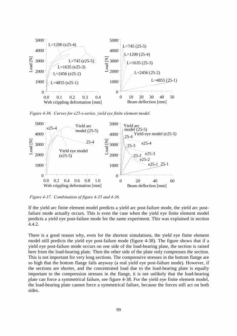
99
0.0 0.1 0.2 0.3 0.4Web crippling deformation [mm]
0
1000
2000
3000
4000
5000
L=4855 (e25-1)
L=2456 (e25-2)L=1635 (e25-3)
L=1200 (e25-4)
L=745 (e25-5)
Load
[N]
0 10 20 30 40 50Beam deflection [mm]
0
1000
2000
3000
4000
5000
L=4855 (25-1)
L=2456 (25-2)
L=1635 (25-3)
L=1200 (25-4)
L=745 (25-5)
Load
[N]
Figure 4-36. Curves for e25-x-series, yield eye finite element model.
0.0 0.2 0.4 0.6 0.8 1.0Web crippling deformation [mm]
0
1000
2000
3000
4000
5000
Yield eye model(e25-5)
Yield arcmodel (25-5)e25-4
25-4
Load
[N]
0 20 40 60Beam deflection [mm]
0
1000
2000
3000
4000
5000
25-1
25-2
25-3
25-4
Yield arcmodel (25-5)
Yield eye model (e25-5)
e25-4
e25-3e25-2
e25-1
Load
[N]
Figure 4-37. Combination of figure 4-35 and 4-36.
If the yield arc finite element model predicts a yield arc post-failure mode, the yield arc post-failure mode actually occurs. This is even the case when the yield eye finite element modelpredicts a yield eye post-failure mode for the same experiment. This was explained in section4.4.2.
There is a good reason why, even for the shortest simulations, the yield eye finite elementmodel still predicts the yield eye post-failure mode (figure 4-38). The figure shows that if ayield eye post-failure mode occurs on one side of the load-bearing plate, the section is raisedhere from the load-bearing plate. Then the other side of the plate only compresses the section.This is not important for very long sections. The compressive stresses in the bottom flange areso high that the bottom flange fails anyway (a real yield eye post-failure mode). However, ifthe sections are shorter, and the concentrated load due to the load-bearing plate is equallyimportant to the compression stresses in the flange, it is not unlikely that the load-bearingplate can force a symmetrical failure, see figure 4-38. For the yield eye finite element model,the load-bearing plate cannot force a symmetrical failure, because the forces still act on bothsides.
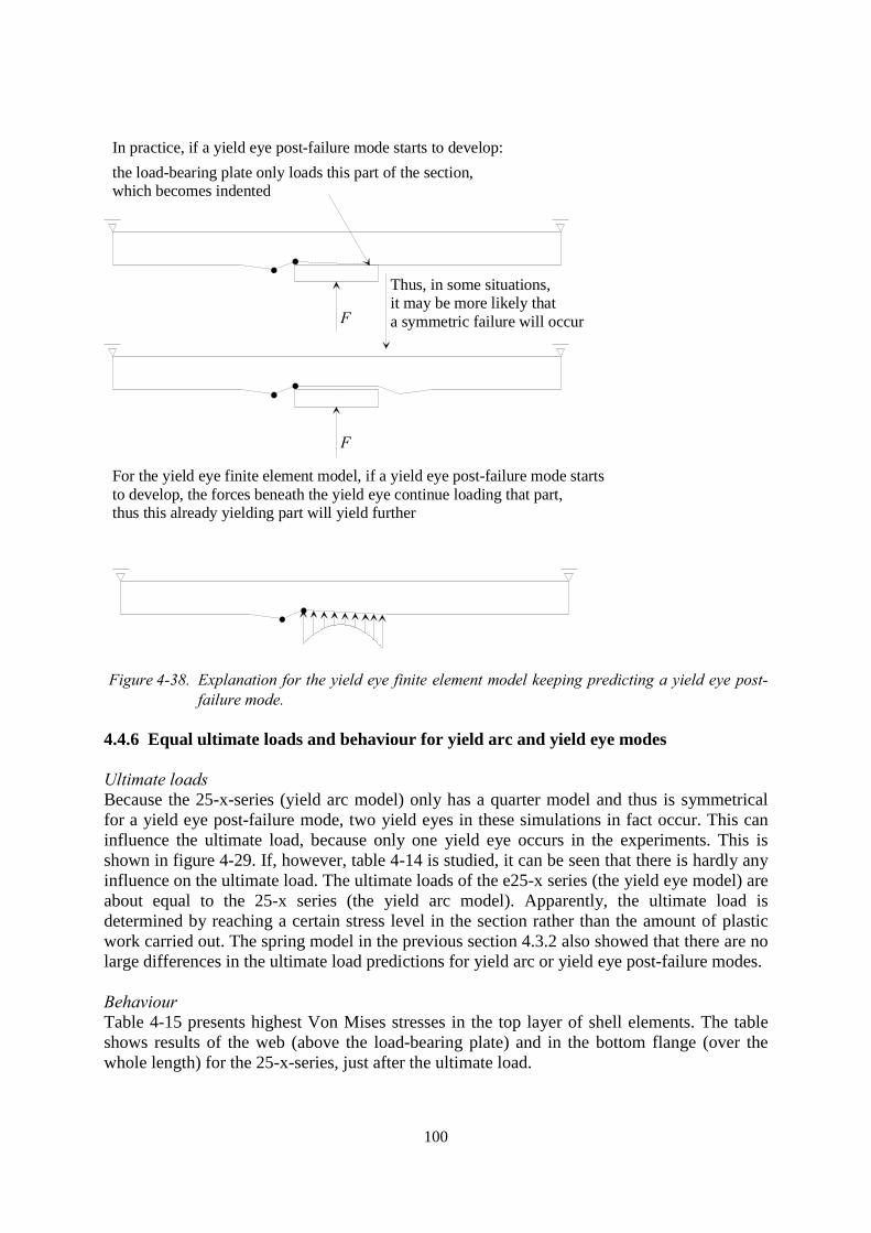
100
In practice, if a yield eye post-failure mode starts to develop:the load-bearing plate only loads this part of the section,which becomes indented
F
F
Thus, in some situations,it may be more likely thata symmetric failure will occur
For the yield eye finite element model, if a yield eye post-failure mode starts to develop, the forces beneath the yield eye continue loading that part,thus this already yielding part will yield further
Figure 4-38. Explanation for the yield eye finite element model keeping predicting a yield eye post-failure mode.
4.4.6 Equal ultimate loads and behaviour for yield arc and yield eye modes
Ultimate loadsBecause the 25-x-series (yield arc model) only has a quarter model and thus is symmetricalfor a yield eye post-failure mode, two yield eyes in these simulations in fact occur. This caninfluence the ultimate load, because only one yield eye occurs in the experiments. This isshown in figure 4-29. If, however, table 4-14 is studied, it can be seen that there is hardly anyinfluence on the ultimate load. The ultimate loads of the e25-x series (the yield eye model) areabout equal to the 25-x series (the yield arc model). Apparently, the ultimate load isdetermined by reaching a certain stress level in the section rather than the amount of plasticwork carried out. The spring model in the previous section 4.3.2 also showed that there are nolarge differences in the ultimate load predictions for yield arc or yield eye post-failure modes.
BehaviourTable 4-15 presents highest Von Mises stresses in the top layer of shell elements. The tableshows results of the web (above the load-bearing plate) and in the bottom flange (over thewhole length) for the 25-x-series, just after the ultimate load.
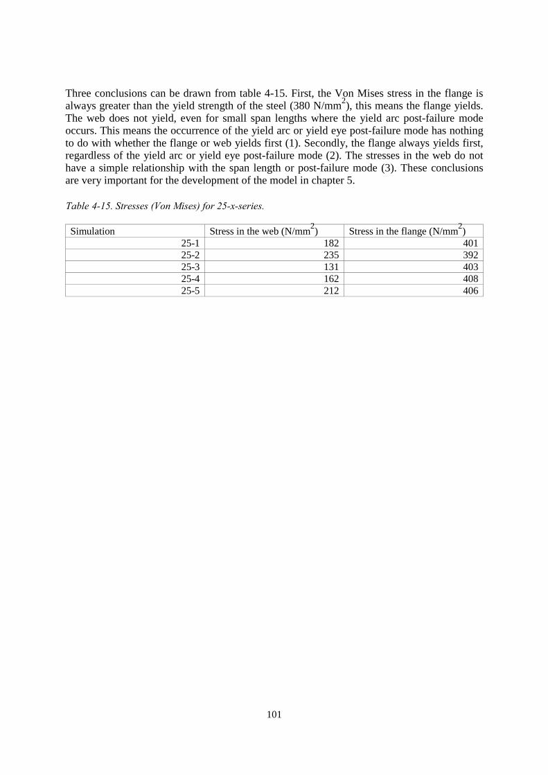
101
Three conclusions can be drawn from table 4-15. First, the Von Mises stress in the flange isalways greater than the yield strength of the steel (380 N/mm2), this means the flange yields.The web does not yield, even for small span lengths where the yield arc post-failure modeoccurs. This means the occurrence of the yield arc or yield eye post-failure mode has nothingto do with whether the flange or web yields first (1). Secondly, the flange always yields first,regardless of the yield arc or yield eye post-failure mode (2). The stresses in the web do nothave a simple relationship with the span length or post-failure mode (3). These conclusionsare very important for the development of the model in chapter 5.
Table 4-15. Stresses (Von Mises) for 25-x-series.
Simulation Stress in the web (N/mm2) Stress in the flange (N/mm2)25-1 182 40125-2 235 39225-3 131 40325-4 162 40825-5 212 406
102
4.5 Conclusions
To simulate the three post-failure modes (yield arc, rolling, and yield eye) found in theexperiments in chapter 3, finite element models were developed. Quarter models were usedfor the yield arc and rolling post-failure modes. For the asymmetric yield eye post-failuremode, a half model was needed. Every post-failure mode requires a specific mesh with a finemesh density where high stress gradients and plastic deformations occur.
For the yield arc and rolling finite element models, loading was applied via a load-bearingplate and contact elements. For the yield eye finite element model, an arc-length method wasneeded and therefore no contact elements could be used. Here, a load is applied by nodalforces, following the elastic force distribution.
Finite element models and experiments agree well for the yield arc and rolling post-failuremodes. This was checked by comparing load deformation curves, yield line patterns, andyield line distances.
For the yield eye post-failure mode, yield line patterns and yield line distances werecomparable for the finite element model and the experiment. Qualitative behaviour wasalways equal for the curves, but the web crippling deformation was different for simulationand experiment. This can be attributed to the difference in load application for the simulationand experiment.
Experiments in chapter 3 showed that there are three post-failure modes after ultimate load.However, the finite element models show that until and at ultimate load, there are only twodifferent failure modes: the "rolling" ultimate failure mode and the "localised yield" failuremode. For the rolling ultimate failure mode, at ultimate load, yield lines in the corner rollthrough corner and web. For the localised yield failure mode at ultimate load, only small yieldspots can be found in the sheet section's bottom corner and flange.
It is not recommended to model the corner radius with only 1 element for experiments failingby the rolling post-failure mode. Modelling the load with prescribed displacements leads to aserious underestimation of the load for experiments failing by the rolling post-failure mode.
In section 4.2.4 it was mentioned that at ultimate load yield arc and yield eye ultimate failuremodes are the same (and both are symmetric). Only after ultimate load are there differences.The yield arc post-failure mode remains symmetric. However, the yield eye post-failure modechanges from symmetric into asymmetric. A spring model was introduced showing that thereis an instantaneous transition between a symmetric and an asymmetric post-failure mode.Thus, after the ultimate load for the yield eye post-failure mode such an instantaneoustransition comes about. During this instant transition, the load-bearing plate contactinstantaneously changes from the whole load-bearing plate to one edge of it. A possiblereason for nonconvergence of the iterative solution is that the steep contact changes cannot befollowed by contact elements.
If a rolling post-failure mode is to be simulated, either a rolling or a yield eye finite elementmodel can be used. For large deformations, the rolling finite element model gives better

103
results, but it does involve longer calculation times. For long span lengths, the yield eye finiteelement model does not converge.
If a yield arc finite element model predicts a symmetric yield eye post-failure mode, it isadvisable to use a yield eye finite element model for this sheet section too. This is not to finda better prediction of the ultimate load, but to produce the correct yield line pattern and yieldline distances.
Both the yield arc and yield eye post-failure mode simulated failed by yielding of the bottomflange first. Both the simulations and the spring model indicated that there are no largedifferences between the ultimate load for yield arc and yield eye post-failure modes.
104
5 Ultimate failure mechanical model
Chapter abstractA mechanical model for the localised yield ultimate failure mode is presented. Themechanical model takes into account the elastic cross-section deformation of a sheet sectiondue to the concentrated load and the buckling of the bottom flange due to compressivestresses caused by the bending moment. The model is compared with the experiments ofchapter 3 and experiments reported in literature. Finally, the accuracy of the model is checkedfor each sheet section variable.

105
Mechanical modelIn this thesis, a mechanical model is a set of equations that predicts the behaviour and/or theultimate load of a sheet section in a three-point bending test. The equations are based onmechanics and are not derived by curve fitting. The main advantage of a mechanical model tocurve-fitting rules is that it gives the user insight into the sheet section behaviour.
Aim of the ultimate failure mechanical modelAn ultimate failure mechanical model was developed for the localised yield ultimate failuremode observed in the finite element simulations (chapter 4). The mechanical model can beused to predict the ultimate load for this ultimate failure mode and thus can serve as a basisfor a design rule.
Structure of this chapterIn section 5.1 the mechanical model is presented and its formulae are derived. The derivationof the formulae is explained in more detail in chapter 1 of a report [Hofm00b]. Section 5.2presents a comparison between the mechanical model and experiments. Section 5.3 comparesthe results according to the mechanical model with those of current design rules.
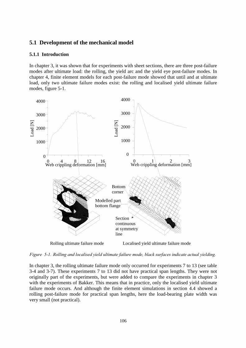
106
5.1 Development of the mechanical model
5.1.1 Introduction
In chapter 3, it was shown that for experiments with sheet sections, there are three post-failuremodes after ultimate load: the rolling, the yield arc and the yield eye post-failure modes. Inchapter 4, finite element models for each post-failure mode showed that until and at ultimateload, only two ultimate failure modes exist: the rolling and localised yield ultimate failuremodes, figure 5-1.
0 4 8 12 16Web crippling deformation [mm]
0
1000
2000
3000
4000
Load
[N]
0 1 2 3Web crippling deformation [mm]
0
1000
2000
3000
4000
Load
[N]
Rolling ultimate failure mode Localised yield ultimate failure mode
Modelled partbottom flange
Sectioncontinuousat symmetryline
Bottomcorner
Figure 5-1. Rolling and localised yield ultimate failure mode, black surfaces indicate actual yielding.
In chapter 3, the rolling ultimate failure mode only occurred for experiments 7 to 13 (see table3-4 and 3-7). These experiments 7 to 13 did not have practical span lengths. They were notoriginally part of the experiments, but were added to compare the experiments in chapter 3with the experiments of Bakker. This means that in practice, only the localised yield ultimatefailure mode occurs. And although the finite element simulations in section 4.4 showed arolling post-failure mode for practical span lengths, here the load-bearing plate width wasvery small (not practical).
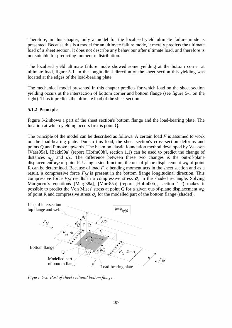
107
Therefore, in this chapter, only a model for the localised yield ultimate failure mode ispresented. Because this is a model for an ultimate failure mode, it merely predicts the ultimateload of a sheet section. It does not describe any behaviour after ultimate load, and therefore isnot suitable for predicting moment redistribution.
The localised yield ultimate failure mode showed some yielding at the bottom corner atultimate load, figure 5-1. In the longitudinal direction of the sheet section this yielding waslocated at the edges of the load-bearing plate.
The mechanical model presented in this chapter predicts for which load on the sheet sectionyielding occurs at the intersection of bottom corner and bottom flange (see figure 5-1 on theright). Thus it predicts the ultimate load of the sheet section.
5.1.2 Principle
Figure 5-2 shows a part of the sheet section's bottom flange and the load-bearing plate. Thelocation at which yielding occurs first is point Q.
The principle of the model can be described as follows. A certain load F is assumed to workon the load-bearing plate. Due to this load, the sheet section's cross-section deforms andpoints Q and P move upwards. The beam on elastic foundation method developed by Vaessen[Vaes95a], [Bakk99a] (report [Hofm00b], section 1.1) can be used to predict the change ofdistances dQ and dP. The difference between these two changes is the out-of-planedisplacement wP of point P. Using a sine function, the out-of-plane displacement wR of pointR can be determined. Because of load F, a bending moment acts in the sheet section and as aresult, a compressive force Fbf is present in the bottom flange longitudinal direction. Thiscompressive force Fbf results in a compressive stress σz in the shaded rectangle. SolvingMarguerre's equations [Marg38a], [Murr85a] (report [Hofm00b], section 1.2) makes itpossible to predict the Von Mises' stress at point Q for a given out-of-plane displacement wRof point R and compressive stress σz for the modelled part of the bottom flange (shaded).
Load-bearing plate
Bottom flange
bFbf /b=σz
P
Q
R
FFbf
Fbf /b
b/2
Line of intersectiontop flange and web
dQ
dP
b=bbf;fl
b
b/2b/2
Fbf
Modelled partof bottom flange
wR
Figure 5-2. Part of sheet sections' bottom flange.
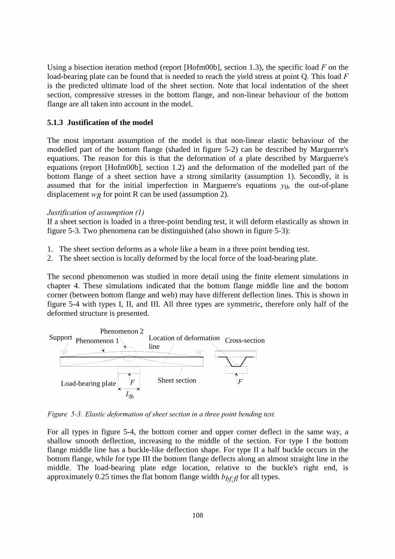
108
Using a bisection iteration method (report [Hofm00b], section 1.3), the specific load F on theload-bearing plate can be found that is needed to reach the yield stress at point Q. This load Fis the predicted ultimate load of the sheet section. Note that local indentation of the sheetsection, compressive stresses in the bottom flange, and non-linear behaviour of the bottomflange are all taken into account in the model.
5.1.3 Justification of the model
The most important assumption of the model is that non-linear elastic behaviour of themodelled part of the bottom flange (shaded in figure 5-2) can be described by Marguerre'sequations. The reason for this is that the deformation of a plate described by Marguerre'sequations (report [Hofm00b], section 1.2) and the deformation of the modelled part of thebottom flange of a sheet section have a strong similarity (assumption 1). Secondly, it isassumed that for the initial imperfection in Marguerre's equations y0, the out-of-planedisplacement wR for point R can be used (assumption 2).
Justification of assumption (1)If a sheet section is loaded in a three-point bending test, it will deform elastically as shown infigure 5-3. Two phenomena can be distinguished (also shown in figure 5-3):
1. The sheet section deforms as a whole like a beam in a three point bending test.2. The sheet section is locally deformed by the local force of the load-bearing plate.
The second phenomenon was studied in more detail using the finite element simulations inchapter 4. These simulations indicated that the bottom flange middle line and the bottomcorner (between bottom flange and web) may have different deflection lines. This is shown infigure 5-4 with types I, II, and III. All three types are symmetric, therefore only half of thedeformed structure is presented.
Load-bearing plate
Support
F F
Cross-section
Sheet section
Location of deformationline
Llb
Phenomenon 1Phenomenon 2
Figure 5-3. Elastic deformation of sheet section in a three point bending test.
For all types in figure 5-4, the bottom corner and upper corner deflect in the same way, ashallow smooth deflection, increasing to the middle of the section. For type I the bottomflange middle line has a buckle-like deflection shape. For type II a half buckle occurs in thebottom flange, while for type III the bottom flange deflects along an almost straight line in themiddle. The load-bearing plate edge location, relative to the buckle's right end, isapproximately 0.25 times the flat bottom flange width bbf;fl for all types.
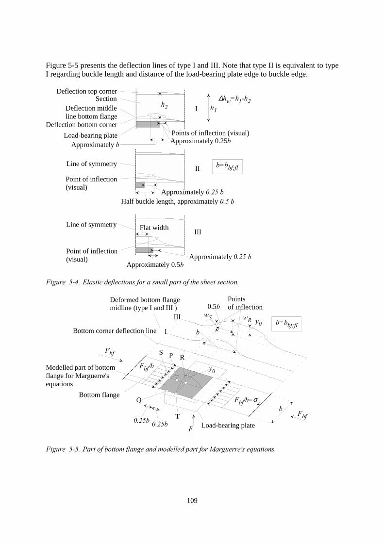
109
Figure 5-5 presents the deflection lines of type I and III. Note that type II is equivalent to typeI regarding buckle length and distance of the load-bearing plate edge to buckle edge.
I
II
III
SectionDeflection top corner
Deflection bottom corner
Deflection middleline bottom flange
Load-bearing plate
Point of inflection(visual)
Approximately b
Half buckle length, approximately 0.5 b
Approximately 0.5b
Approximately 0.25 b
Approximately 0.25 b
Approximately 0.25b
Line of symmetry
Points of inflection (visual)
Point of inflection(visual)
Line of symmetry Flat width
b=bbf;fl
h2 h1
∆hw=h1-h2
Figure 5-4. Elastic deflections for a small part of the sheet section.
Deformed bottom flange midline (type I and III )
I
III
0.25b
Pointsof inflection
Load-bearing plate
Bottom flange
b
Fbf
Fbf/b=σz
P
Q
F
Ry0
wR
S
wS y0
Modelled part of bottomflange for Marguerre'sequations
Bottom corner deflection line
Fbf/b
b
0.5b
b=bbf;fl
0.25bT Fbf
Figure 5-5. Part of bottom flange and modelled part for Marguerre's equations.
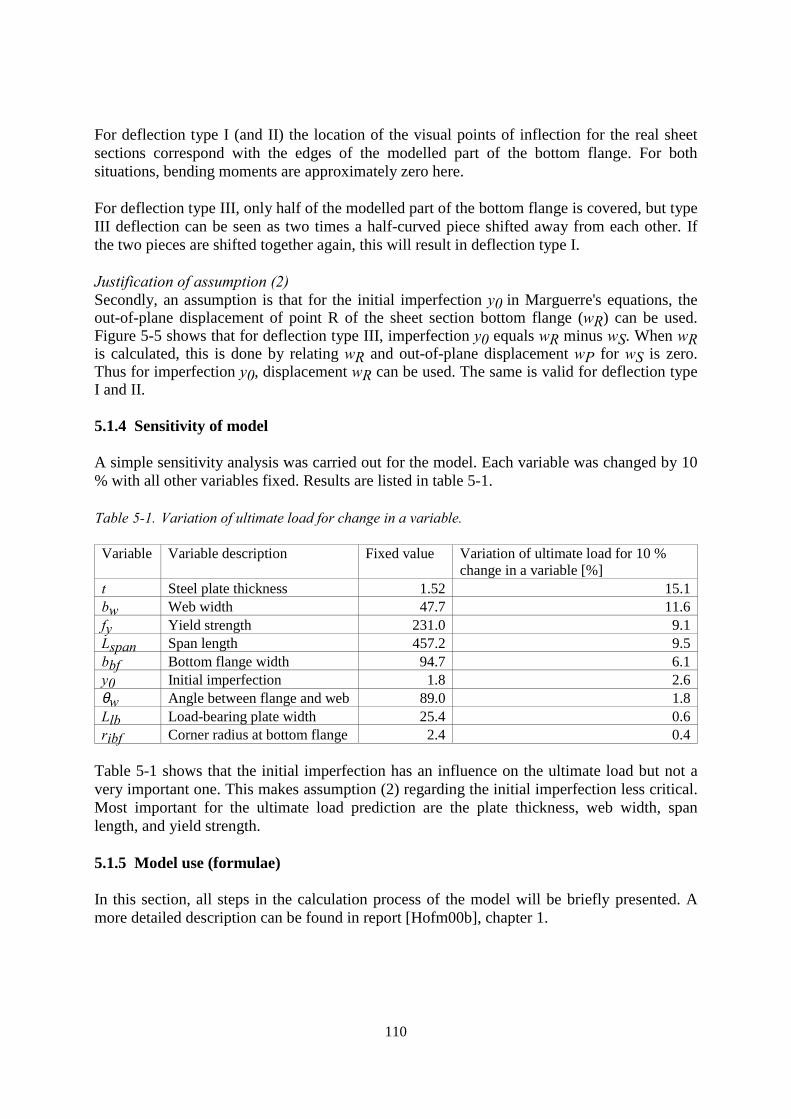
110
For deflection type I (and II) the location of the visual points of inflection for the real sheetsections correspond with the edges of the modelled part of the bottom flange. For bothsituations, bending moments are approximately zero here.
For deflection type III, only half of the modelled part of the bottom flange is covered, but typeIII deflection can be seen as two times a half-curved piece shifted away from each other. Ifthe two pieces are shifted together again, this will result in deflection type I.
Justification of assumption (2)Secondly, an assumption is that for the initial imperfection y0 in Marguerre's equations, theout-of-plane displacement of point R of the sheet section bottom flange (wR) can be used.Figure 5-5 shows that for deflection type III, imperfection y0 equals wR minus wS. When wRis calculated, this is done by relating wR and out-of-plane displacement wP for wS is zero.Thus for imperfection y0, displacement wR can be used. The same is valid for deflection typeI and II.
5.1.4 Sensitivity of model
A simple sensitivity analysis was carried out for the model. Each variable was changed by 10% with all other variables fixed. Results are listed in table 5-1.
Table 5-1. Variation of ultimate load for change in a variable.
Variable Variable description Fixed value Variation of ultimate load for 10 %change in a variable [%]
t Steel plate thickness 1.52 15.1bw Web width 47.7 11.6fy Yield strength 231.0 9.1Lspan Span length 457.2 9.5bbf Bottom flange width 94.7 6.1y0 Initial imperfection 1.8 2.6θw Angle between flange and web 89.0 1.8Llb Load-bearing plate width 25.4 0.6ribf Corner radius at bottom flange 2.4 0.4
Table 5-1 shows that the initial imperfection has an influence on the ultimate load but not avery important one. This makes assumption (2) regarding the initial imperfection less critical.Most important for the ultimate load prediction are the plate thickness, web width, spanlength, and yield strength.
5.1.5 Model use (formulae)
In this section, all steps in the calculation process of the model will be briefly presented. Amore detailed description can be found in report [Hofm00b], chapter 1.
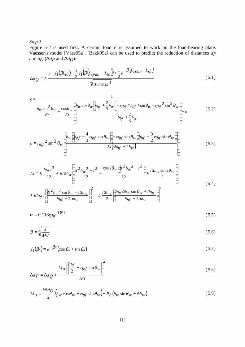
111
Step 1Figure 5-2 is used first. A certain load F is assumed to work on the load-bearing plate.Vaessen's model [Vaes95a], [Bakk99a] can be used to predict the reduction of distances dPand dQ (∆dP and ∆dQ):
( ) ( )( ) ( )4 31024
21
121
11
EIk
lbLspanLelbLspanLflbLf
FQd
−−+−−+
=∆
βββ
( 5.1)
bwbbfb
wibfrwbfbibfrwbbfbwwb
Etw
Etwwb
k
+
+
−+
+
+
=
32
2sin2sin**32cos
cos2sin
1
θθθθθ ( 5.2)
( )
+
−+
−
=wbbfbEt
wibfrbfbwibfrwibfrbfbwbwibfrb
23
sin23sinsin
34
2sin2θθθ
θ ( 5.3)
2
2
sin
2
2
2sin22
22sin
12
2222cos
12
222
12
3
+
++
++
+
+
−−
++=
wbbfbbftbwwbbfbwbt
Ewbbfb
wbtwwbtbfEb
wwbttwbwtwbwbEt
tbfbEEI
α
θααα
αθα
θααθαα
( 5.4)
89.0118.0 ibfr=α ( 5.5)
44EI
k=β ( 5.6)
( ) ( )xxxexf ββββ sincos1 +−= ( 5.7)
EI
wibfrbfbaM
QdPd2
2sin
2
−
+∆=∆
θ ( 5.8)
( ) ( )whwwbhRwibfrwwbQdkaM ∆−−+
∆= θθθ sinsincos
2( 5.9)
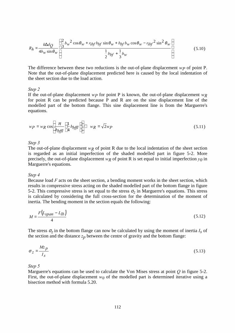
112
+
−++∆=
wbbfb
wibfrwwbbfbwbfbibfrwwb
wwbQdk
hR
31
21
2sin2cossincos232
sin4
θθθθ
θ (5.10)
The difference between these two reductions is the out-of-plane displacement wP of point P.Note that the out-of-plane displacement predicted here is caused by the local indentation ofthe sheet section due to the load action.
Step 2If the out-of-plane displacement wP for point P is known, the out-of-plane displacement wRfor point R can be predicted because P and R are on the sine displacement line of themodelled part of the bottom flange. This sine displacement line is from the Marguerre'sequations.
PwRwbfflbbfflbRwPw 2
41cos =⇔
= π (5.11)
Step 3The out-of-plane displacement wR of point R due to the local indentation of the sheet sectionis regarded as an initial imperfection of the shaded modelled part in figure 5-2. Moreprecisely, the out-of-plane displacement wR of point R is set equal to initial imperfection y0 inMarguerre's equations.
Step 4Because load F acts on the sheet section, a bending moment works in the sheet section, whichresults in compressive stress acting on the shaded modelled part of the bottom flange in figure5-2. This compressive stress is set equal to the stress σz in Marguerre's equations. This stressis calculated by considering the full cross-section for the determination of the moment ofinertia. The bending moment in the section equals the following:
( )4
lbLspanLFM
−= (5.12)
The stress σz in the bottom flange can now be calculated by using the moment of inertia Is ofthe section and the distance zp between the centre of gravity and the bottom flange:
sIpMz
z =σ (5.13)
Step 5Marguerre's equations can be used to calculate the Von Mises stress at point Q in figure 5-2.First, the out-of-plane displacement w0 of the modelled part is determined iterative using abisection method with formula 5.20.
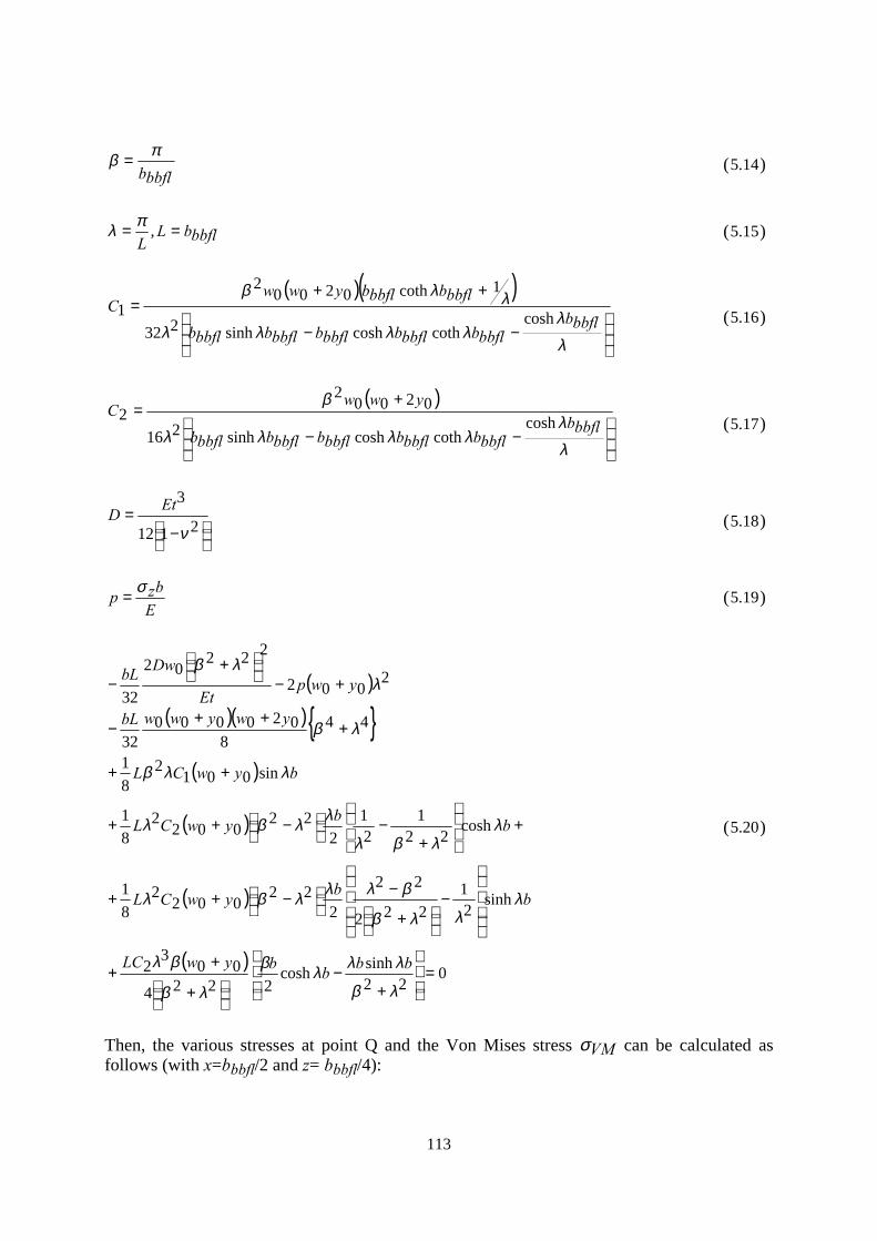
113
bbflbπβ = (5.14)
bbflbLL
== ,πλ (5.15)
( )( )
−−
++=
λλ
λλλλ
λλβ
bbflbbbflbbbflbbbflbbbflbbbflb
bbflbbbflbywwC
coshcothcoshsinh232
1coth02002
1 (5.16)
( )
−−
+=
λλ
λλλλ
β
bbflbbbflbbbflbbbflbbbflbbbflb
ywwC
coshcothcoshsinh216
02002
2 (5.17)
−=
2112
3
ν
EtD (5.18)
Ebzp σ= (5.19)
( )( )( ){ }
( )
( )
( )
( )0
22sinhcosh
222400
32
sinh21
222
22
222
0022
81
cosh22
121
222
0022
81
sin0012
81
448
02000032
2002
22202
32
=
+−
+
++
−
+
−
−++
+
+−
−++
++
+++
−
+−
+−
λβ
λλλβ
λβ
βλ
λλλβ
βλλλβλ
λλβλ
λλβλ
λλβ
λβ
λλβ
bbbbywLC
bbywCL
bbywCL
bywCL
ywywwbL
ywpEt
DwbL
(5.20)
Then, the various stresses at point Q and the Von Mises stress σVM can be calculated asfollows (with x=bbbfl/2 and z= bbbfl/4):
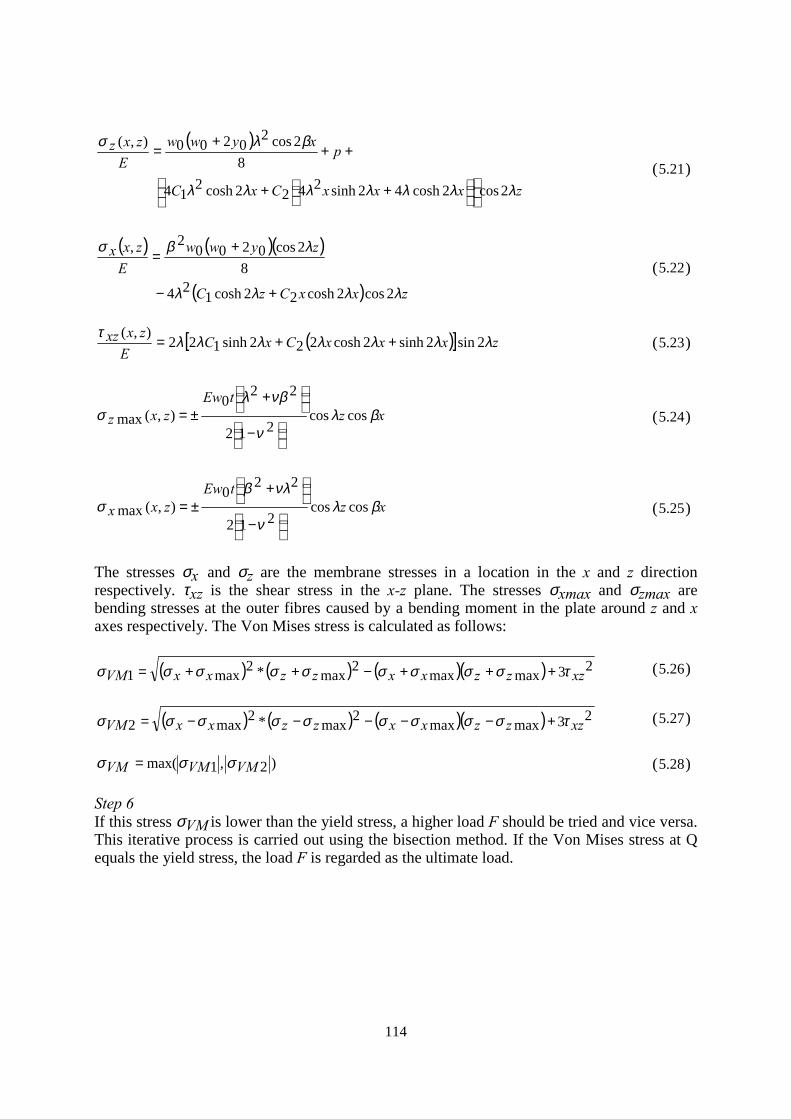
114
( )
zxxxCxC
pxyww
Ezxz
λλλλλλλ
βλσ
2cos2cosh42sinh2422cosh214
82cos2
0200),(
++
+++
=(5.21)
( ) ( )( )
( ) zxxCzC
zywwE
zxx
λλλλ
λβσ
2cos2cosh22cosh124
82cos0200
2,
+−
+=
(5.22)
( )[ ] zxxxCxCE
zxxz λλλλλλλτ
2sin2sinh2cosh222sinh122),(
++= (5.23)
xztEw
zxz βλν
νβλσ coscos
212
220
),(max
−
+±= (5.24)
xztEw
zxx βλν
νλβσ coscos
212
220
),(max
−
+±= (5.25)
The stresses σx and σz are the membrane stresses in a location in the x and z directionrespectively. τxz is the shear stress in the x-z plane. The stresses σxmax and σzmax arebending stresses at the outer fibres caused by a bending moment in the plate around z and xaxes respectively. The Von Mises stress is calculated as follows:
( ) ( ) ( )( ) 23maxmax2
max*2max1 xzzzxxzzxxVM τσσσσσσσσσ +++−++= (5.26)
( ) ( ) ( )( ) 23maxmax2
max*2max2 xzzzxxzzxxVM τσσσσσσσσσ +−−−−−= (5.27)
)2,1max( VMVMVM σσσ = (5.28)
Step 6If this stress σVM is lower than the yield stress, a higher load F should be tried and vice versa.This iterative process is carried out using the bisection method. If the Von Mises stress at Qequals the yield stress, the load F is regarded as the ultimate load.
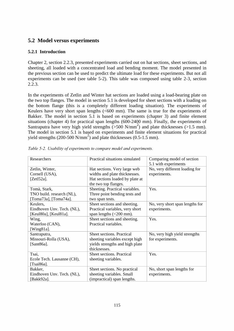
115
5.2 Model versus experiments
5.2.1 Introduction
Chapter 2, section 2.2.3, presented experiments carried out on hat sections, sheet sections, andsheeting, all loaded with a concentrated load and bending moment. The model presented inthe previous section can be used to predict the ultimate load for these experiments. But not allexperiments can be used (see table 5-2). This table was composed using table 2-3, section2.2.3.
In the experiments of Zetlin and Winter hat sections are loaded using a load-bearing plate onthe two top flanges. The model in section 5.1 is developed for sheet sections with a loading onthe bottom flange (this is a completely different loading situation). The experiments ofKeulers have very short span lengths (<600 mm). The same is true for the experiments ofBakker. The model in section 5.1 is based on experiments (chapter 3) and finite elementsituations (chapter 4) for practical span lengths (600-2400 mm). Finally, the experiments ofSantraputra have very high yield strengths (>500 N/mm2) and plate thicknesses (>1.5 mm).The model in section 5.1 is based on experiments and finite element situations for practicalyield strengths (200-500 N/mm2) and plate thicknesses (0.5-1.5 mm).
Table 5-2. Usability of experiments to compare model and experiments.
Researchers Practical situations simulated Comparing model of section5.1 with experiments
Zetlin, Winter,Cornell (USA),[Zetl52a].
Hat sections. Very large webwidths and plate thicknesses.Hat sections loaded by plate atthe two top flanges.
No, very different loading forexperiments.
Tomà, Stark,TNO build. research (NL),[Toma73a], [Toma74a].
Sheeting. Practical variables.Three point bending tests andtwo span tests.
Yes.
Keulers,Eindhoven Unv. Tech. (NL),[Keul80a], [Keul81a].
Sheet sections and sheeting.Practical variables, very shortspan lengths (<200 mm).
No, very short span lengths forexperiments.
Wing,Waterloo (CAN),[Wing81a].
Sheet sections and sheeting.Practical variables.
Yes.
Santraputra,Missouri-Rolla (USA),[Sant86a].
Sheet sections. Practicalsheeting variables except highyields strengths and high platethicknesses.
No, very high yield strengthsfor experiments.
Tsai,Ecole Tech. Lausanne (CH),[Tsai86a].
Sheet sections. Practicalsheeting variables.
Yes.
Bakker,Eindhoven Unv. Tech. (NL),[Bakk92a].
Sheet sections. No practicalsheeting variables. Small(impractical) span lengths.
No, short span lengths forexperiments.
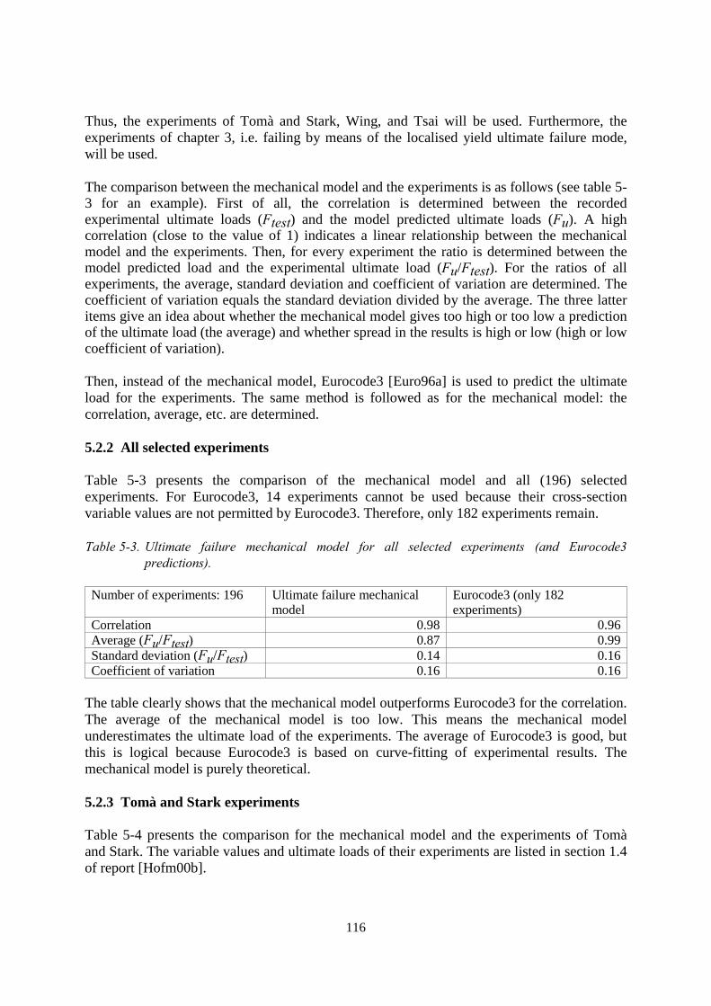
116
Thus, the experiments of Tomà and Stark, Wing, and Tsai will be used. Furthermore, theexperiments of chapter 3, i.e. failing by means of the localised yield ultimate failure mode,will be used.
The comparison between the mechanical model and the experiments is as follows (see table 5-3 for an example). First of all, the correlation is determined between the recordedexperimental ultimate loads (Ftest) and the model predicted ultimate loads (Fu). A highcorrelation (close to the value of 1) indicates a linear relationship between the mechanicalmodel and the experiments. Then, for every experiment the ratio is determined between themodel predicted load and the experimental ultimate load (Fu/Ftest). For the ratios of allexperiments, the average, standard deviation and coefficient of variation are determined. Thecoefficient of variation equals the standard deviation divided by the average. The three latteritems give an idea about whether the mechanical model gives too high or too low a predictionof the ultimate load (the average) and whether spread in the results is high or low (high or lowcoefficient of variation).
Then, instead of the mechanical model, Eurocode3 [Euro96a] is used to predict the ultimateload for the experiments. The same method is followed as for the mechanical model: thecorrelation, average, etc. are determined.
5.2.2 All selected experiments
Table 5-3 presents the comparison of the mechanical model and all (196) selectedexperiments. For Eurocode3, 14 experiments cannot be used because their cross-sectionvariable values are not permitted by Eurocode3. Therefore, only 182 experiments remain.
Table 5-3. Ultimate failure mechanical model for all selected experiments (and Eurocode3predictions).
Number of experiments: 196 Ultimate failure mechanicalmodel
Eurocode3 (only 182experiments)
Correlation 0.98 0.96Average (Fu/Ftest) 0.87 0.99Standard deviation (Fu/Ftest) 0.14 0.16Coefficient of variation 0.16 0.16
The table clearly shows that the mechanical model outperforms Eurocode3 for the correlation.The average of the mechanical model is too low. This means the mechanical modelunderestimates the ultimate load of the experiments. The average of Eurocode3 is good, butthis is logical because Eurocode3 is based on curve-fitting of experimental results. Themechanical model is purely theoretical.
5.2.3 Tomà and Stark experiments
Table 5-4 presents the comparison for the mechanical model and the experiments of Tomàand Stark. The variable values and ultimate loads of their experiments are listed in section 1.4of report [Hofm00b].
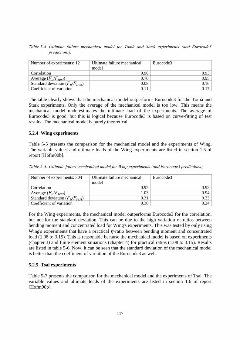
117
Table 5-4. Ultimate failure mechanical model for Tomà and Stark experiments (and Eurocode3predictions).
Number of experiments: 12 Ultimate failure mechanicalmodel
Eurocode3
Correlation 0.96 0.93Average (Fu/Ftest) 0.70 0.95Standard deviation (Fu/Ftest) 0.08 0.16Coefficient of variation 0.11 0.17
The table clearly shows that the mechanical model outperforms Eurocode3 for the Tomà andStark experiments. Only the average of the mechanical model is too low. This means themechanical model underestimates the ultimate load of the experiments. The average ofEurocode3 is good, but this is logical because Eurocode3 is based on curve-fitting of testresults. The mechanical model is purely theoretical.
5.2.4 Wing experiments
Table 5-5 presents the comparison for the mechanical model and the experiments of Wing.The variable values and ultimate loads of the Wing experiments are listed in section 1.5 ofreport [Hofm00b].
Table 5-5. Ultimate failure mechanical model for Wing experiments (and Eurocode3 predictions).
Number of experiments: 304 Ultimate failure mechanicalmodel
Eurocode3
Correlation 0.95 0.92Average (Fu/Ftest) 1.03 0.94Standard deviation (Fu/Ftest) 0.31 0.23Coefficient of variation 0.30 0.24
For the Wing experiments, the mechanical model outperforms Eurocode3 for the correlation,but not for the standard deviation. This can be due to the high variation of ratios betweenbending moment and concentrated load for Wing's experiments. This was tested by only usingWing's experiments that have a practical η-ratio between bending moment and concentratedload (1.08 to 3.15). This is reasonable because the mechanical model is based on experiments(chapter 3) and finite element situations (chapter 4) for practical ratios (1.08 to 3.15). Resultsare listed in table 5-6. Now, it can be seen that the standard deviation of the mechanical modelis better than the coefficient of variation of the Eurocode3 as well.
5.2.5 Tsai experiments
Table 5-7 presents the comparison for the mechanical model and the experiments of Tsai. Thevariable values and ultimate loads of the experiments are listed in section 1.6 of report[Hofm00b].
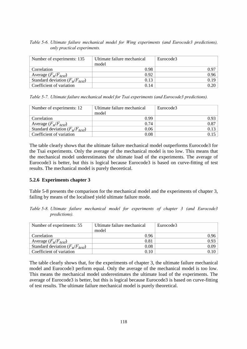
118
Table 5-6. Ultimate failure mechanical model for Wing experiments (and Eurocode3 predictions),only practical experiments.
Number of experiments: 135 Ultimate failure mechanicalmodel
Eurocode3
Correlation 0.98 0.97Average (Fu/Ftest) 0.92 0.96Standard deviation (Fu/Ftest) 0.13 0.19Coefficient of variation 0.14 0.20
Table 5-7. Ultimate failure mechanical model for Tsai experiments (and Eurocode3 predictions).
Number of experiments: 12 Ultimate failure mechanicalmodel
Eurocode3
Correlation 0.99 0.93Average (Fu/Ftest) 0.74 0.87Standard deviation (Fu/Ftest) 0.06 0.13Coefficient of variation 0.08 0.15
The table clearly shows that the ultimate failure mechanical model outperforms Eurocode3 forthe Tsai experiments. Only the average of the mechanical model is too low. This means thatthe mechanical model underestimates the ultimate load of the experiments. The average ofEurocode3 is better, but this is logical because Eurocode3 is based on curve-fitting of testresults. The mechanical model is purely theoretical.
5.2.6 Experiments chapter 3
Table 5-8 presents the comparison for the mechanical model and the experiments of chapter 3,failing by means of the localised yield ultimate failure mode.
Table 5-8. Ultimate failure mechanical model for experiments of chapter 3 (and Eurocode3predictions).
Number of experiments: 55 Ultimate failure mechanicalmodel
Eurocode3
Correlation 0.96 0.96Average (Fu/Ftest) 0.81 0.93Standard deviation (Fu/Ftest) 0.08 0.09Coefficient of variation 0.10 0.10
The table clearly shows that, for the experiments of chapter 3, the ultimate failure mechanicalmodel and Eurocode3 perform equal. Only the average of the mechanical model is too low.This means the mechanical model underestimates the ultimate load of the experiments. Theaverage of Eurocode3 is better, but this is logical because Eurocode3 is based on curve-fittingof test results. The ultimate failure mechanical model is purely theoretical.
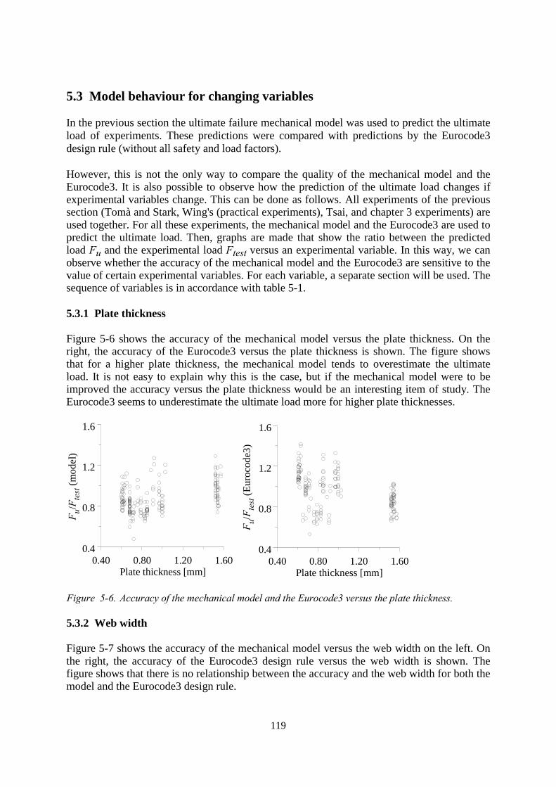
119
5.3 Model behaviour for changing variables
In the previous section the ultimate failure mechanical model was used to predict the ultimateload of experiments. These predictions were compared with predictions by the Eurocode3design rule (without all safety and load factors).
However, this is not the only way to compare the quality of the mechanical model and theEurocode3. It is also possible to observe how the prediction of the ultimate load changes ifexperimental variables change. This can be done as follows. All experiments of the previoussection (Tomà and Stark, Wing's (practical experiments), Tsai, and chapter 3 experiments) areused together. For all these experiments, the mechanical model and the Eurocode3 are used topredict the ultimate load. Then, graphs are made that show the ratio between the predictedload Fu and the experimental load Ftest versus an experimental variable. In this way, we canobserve whether the accuracy of the mechanical model and the Eurocode3 are sensitive to thevalue of certain experimental variables. For each variable, a separate section will be used. Thesequence of variables is in accordance with table 5-1.
5.3.1 Plate thickness
Figure 5-6 shows the accuracy of the mechanical model versus the plate thickness. On theright, the accuracy of the Eurocode3 versus the plate thickness is shown. The figure showsthat for a higher plate thickness, the mechanical model tends to overestimate the ultimateload. It is not easy to explain why this is the case, but if the mechanical model were to beimproved the accuracy versus the plate thickness would be an interesting item of study. TheEurocode3 seems to underestimate the ultimate load more for higher plate thicknesses.
0.40 0.80 1.20 1.60Plate thickness [mm]
0.4
0.8
1.2
1.6
F u/F te
st (m
odel
)
0.40 0.80 1.20 1.60Plate thickness [mm]
0.4
0.8
1.2
1.6
F u/F te
st (E
uroc
ode3
)
Figure 5-6. Accuracy of the mechanical model and the Eurocode3 versus the plate thickness.
5.3.2 Web width
Figure 5-7 shows the accuracy of the mechanical model versus the web width on the left. Onthe right, the accuracy of the Eurocode3 design rule versus the web width is shown. Thefigure shows that there is no relationship between the accuracy and the web width for both themodel and the Eurocode3 design rule.
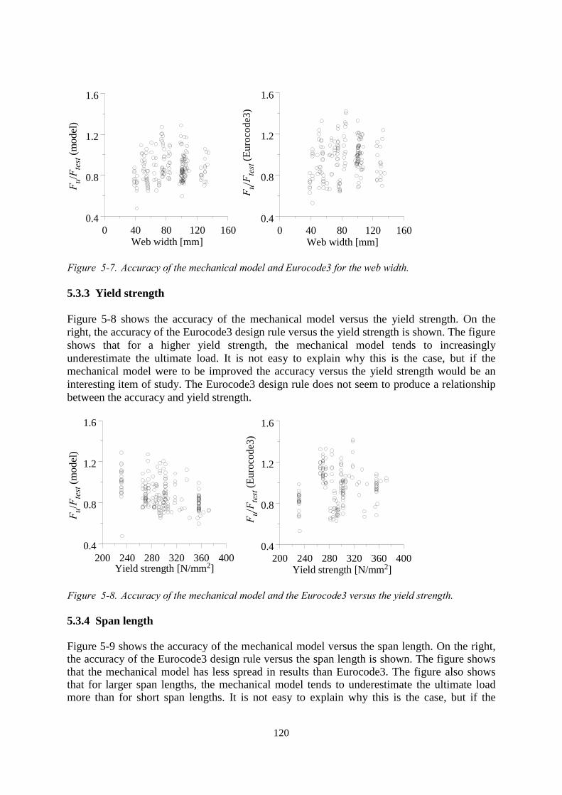
120
0 40 80 120 160Web width [mm]
0.4
0.8
1.2
1.6
F u/F te
st (m
odel
)
0 40 80 120 160Web width [mm]
0.4
0.8
1.2
1.6
F u/F te
st (E
uroc
ode3
)
Figure 5-7. Accuracy of the mechanical model and Eurocode3 for the web width.
5.3.3 Yield strength
Figure 5-8 shows the accuracy of the mechanical model versus the yield strength. On theright, the accuracy of the Eurocode3 design rule versus the yield strength is shown. The figureshows that for a higher yield strength, the mechanical model tends to increasinglyunderestimate the ultimate load. It is not easy to explain why this is the case, but if themechanical model were to be improved the accuracy versus the yield strength would be aninteresting item of study. The Eurocode3 design rule does not seem to produce a relationshipbetween the accuracy and yield strength.
200 240 280 320 360 400Yield strength [N/mm2]
0.4
0.8
1.2
1.6
F u/F te
st (m
odel
)
200 240 280 320 360 400Yield strength [N/mm2]
0.4
0.8
1.2
1.6
F u/F te
st (E
uroc
ode3
)
Figure 5-8. Accuracy of the mechanical model and the Eurocode3 versus the yield strength.
5.3.4 Span length
Figure 5-9 shows the accuracy of the mechanical model versus the span length. On the right,the accuracy of the Eurocode3 design rule versus the span length is shown. The figure showsthat the mechanical model has less spread in results than Eurocode3. The figure also showsthat for larger span lengths, the mechanical model tends to underestimate the ultimate loadmore than for short span lengths. It is not easy to explain why this is the case, but if the
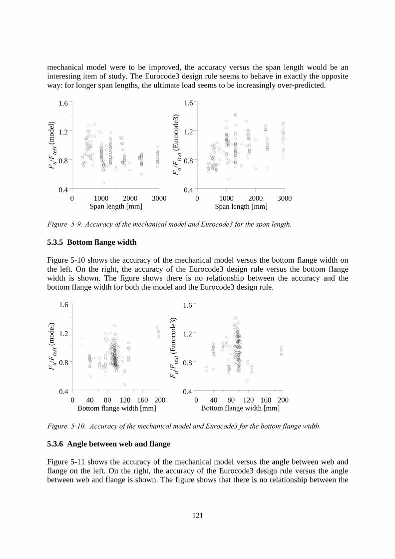
121
mechanical model were to be improved, the accuracy versus the span length would be aninteresting item of study. The Eurocode3 design rule seems to behave in exactly the oppositeway: for longer span lengths, the ultimate load seems to be increasingly over-predicted.
0 1000 2000 3000Span length [mm]
0.4
0.8
1.2
1.6
F u/F te
st (m
odel
)
0 1000 2000 3000Span length [mm]
0.4
0.8
1.2
1.6
F u/F te
st (E
uroc
ode3
)
Figure 5-9. Accuracy of the mechanical model and Eurocode3 for the span length.
5.3.5 Bottom flange width
Figure 5-10 shows the accuracy of the mechanical model versus the bottom flange width onthe left. On the right, the accuracy of the Eurocode3 design rule versus the bottom flangewidth is shown. The figure shows there is no relationship between the accuracy and thebottom flange width for both the model and the Eurocode3 design rule.
0 40 80 120 160 200Bottom flange width [mm]
0.4
0.8
1.2
1.6
F u/F te
st (m
odel
)
0 40 80 120 160 200Bottom flange width [mm]
0.4
0.8
1.2
1.6
F u/F te
st (E
uroc
ode3
)
Figure 5-10. Accuracy of the mechanical model and Eurocode3 for the bottom flange width.
5.3.6 Angle between web and flange
Figure 5-11 shows the accuracy of the mechanical model versus the angle between web andflange on the left. On the right, the accuracy of the Eurocode3 design rule versus the anglebetween web and flange is shown. The figure shows that there is no relationship between the
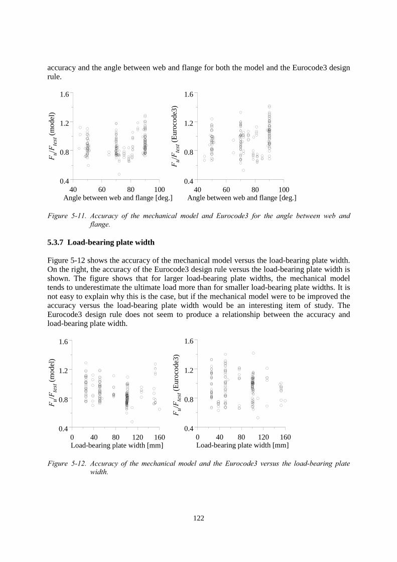
122
accuracy and the angle between web and flange for both the model and the Eurocode3 designrule.
40 60 80 100Angle between web and flange [deg.]
0.4
0.8
1.2
1.6
F u/F te
st (m
odel
)
40 60 80 100Angle between web and flange [deg.]
0.4
0.8
1.2
1.6
F u/F te
st (E
uroc
ode3
)
Figure 5-11. Accuracy of the mechanical model and Eurocode3 for the angle between web andflange.
5.3.7 Load-bearing plate width
Figure 5-12 shows the accuracy of the mechanical model versus the load-bearing plate width.On the right, the accuracy of the Eurocode3 design rule versus the load-bearing plate width isshown. The figure shows that for larger load-bearing plate widths, the mechanical modeltends to underestimate the ultimate load more than for smaller load-bearing plate widths. It isnot easy to explain why this is the case, but if the mechanical model were to be improved theaccuracy versus the load-bearing plate width would be an interesting item of study. TheEurocode3 design rule does not seem to produce a relationship between the accuracy andload-bearing plate width.
0 40 80 120 160Load-bearing plate width [mm]
0.4
0.8
1.2
1.6
F u/F te
st (m
odel
)
0 40 80 120 160Load-bearing plate width [mm]
0.4
0.8
1.2
1.6
F u/F te
st (E
uroc
ode3
)
Figure 5-12. Accuracy of the mechanical model and the Eurocode3 versus the load-bearing platewidth.
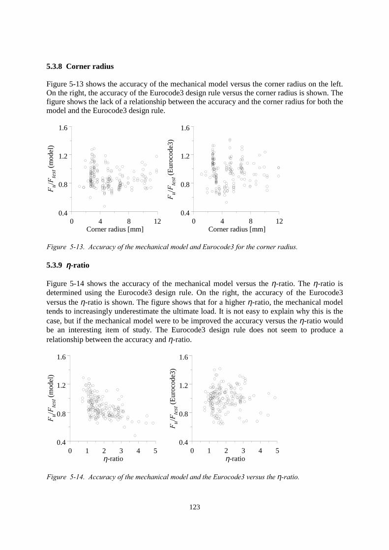
123
5.3.8 Corner radius
Figure 5-13 shows the accuracy of the mechanical model versus the corner radius on the left.On the right, the accuracy of the Eurocode3 design rule versus the corner radius is shown. Thefigure shows the lack of a relationship between the accuracy and the corner radius for both themodel and the Eurocode3 design rule.
0 4 8 12Corner radius [mm]
0.4
0.8
1.2
1.6
F u/F te
st (m
odel
)
0 4 8 12Corner radius [mm]
0.4
0.8
1.2
1.6
F u/F te
st (E
uroc
ode3
)
Figure 5-13. Accuracy of the mechanical model and Eurocode3 for the corner radius.
5.3.9 ηηηη-ratio
Figure 5-14 shows the accuracy of the mechanical model versus the η-ratio. The η-ratio isdetermined using the Eurocode3 design rule. On the right, the accuracy of the Eurocode3versus the η-ratio is shown. The figure shows that for a higher η-ratio, the mechanical modeltends to increasingly underestimate the ultimate load. It is not easy to explain why this is thecase, but if the mechanical model were to be improved the accuracy versus the η-ratio wouldbe an interesting item of study. The Eurocode3 design rule does not seem to produce arelationship between the accuracy and η-ratio.
0 1 2 3 4 5η-ratio
0.4
0.8
1.2
1.6
F u/F te
st (m
odel
)
0 1 2 3 4 5η-ratio
0.4
0.8
1.2
1.6
F u/F te
st (E
uroc
ode3
)
Figure 5-14. Accuracy of the mechanical model and the Eurocode3 versus the η-ratio.
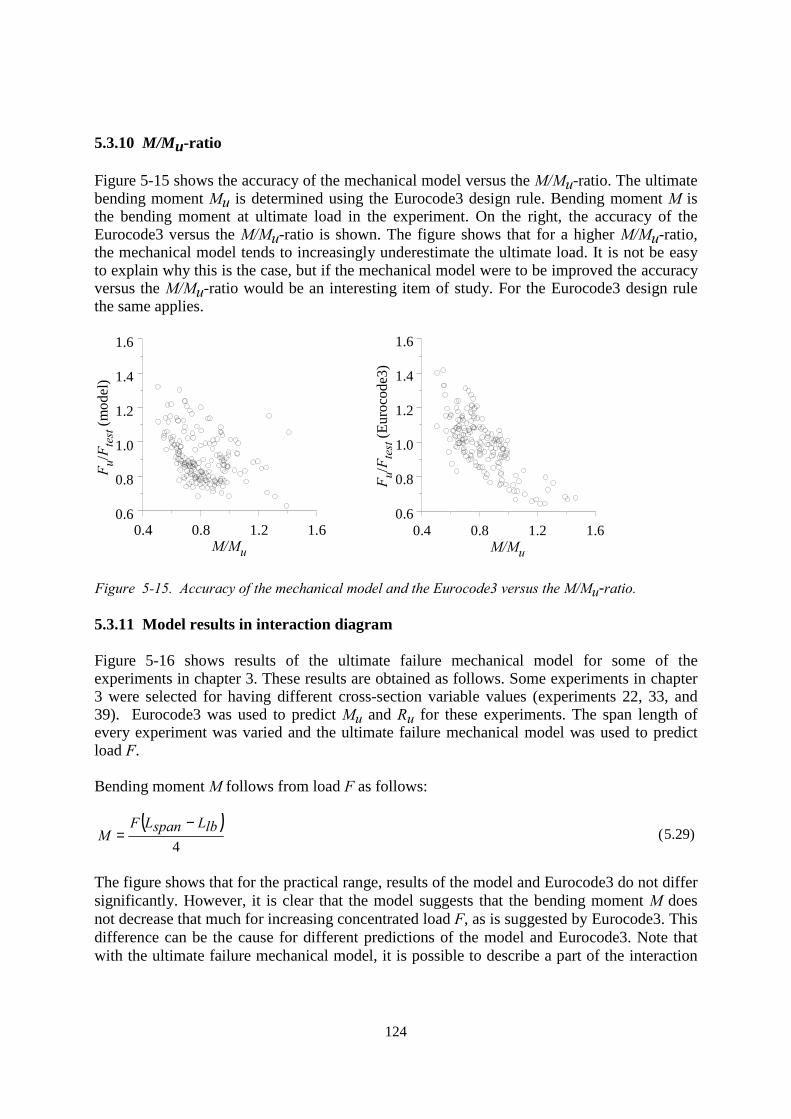
124
5.3.10 M/Mu-ratio
Figure 5-15 shows the accuracy of the mechanical model versus the M/Mu-ratio. The ultimatebending moment Mu is determined using the Eurocode3 design rule. Bending moment M isthe bending moment at ultimate load in the experiment. On the right, the accuracy of theEurocode3 versus the M/Mu-ratio is shown. The figure shows that for a higher M/Mu-ratio,the mechanical model tends to increasingly underestimate the ultimate load. It is not be easyto explain why this is the case, but if the mechanical model were to be improved the accuracyversus the M/Mu-ratio would be an interesting item of study. For the Eurocode3 design rulethe same applies.
0.4 0.8 1.2 1.6M/Mu
F u/F te
st (m
odel
)
0.4 0.8 1.2 1.60.6
0.8
1.0
1.2
1.4
1.6
F u/F te
st (E
uroc
ode3
)
M/Mu
0.6
0.8
1.0
1.2
1.4
1.6
Figure 5-15. Accuracy of the mechanical model and the Eurocode3 versus the M/Mu-ratio.
5.3.11 Model results in interaction diagram
Figure 5-16 shows results of the ultimate failure mechanical model for some of theexperiments in chapter 3. These results are obtained as follows. Some experiments in chapter3 were selected for having different cross-section variable values (experiments 22, 33, and39). Eurocode3 was used to predict Mu and Ru for these experiments. The span length ofevery experiment was varied and the ultimate failure mechanical model was used to predictload F.
Bending moment M follows from load F as follows:
( )4
lbLspanLFM
−= (5.29)
The figure shows that for the practical range, results of the model and Eurocode3 do not differsignificantly. However, it is clear that the model suggests that the bending moment M doesnot decrease that much for increasing concentrated load F, as is suggested by Eurocode3. Thisdifference can be the cause for different predictions of the model and Eurocode3. Note thatwith the ultimate failure mechanical model, it is possible to describe a part of the interaction
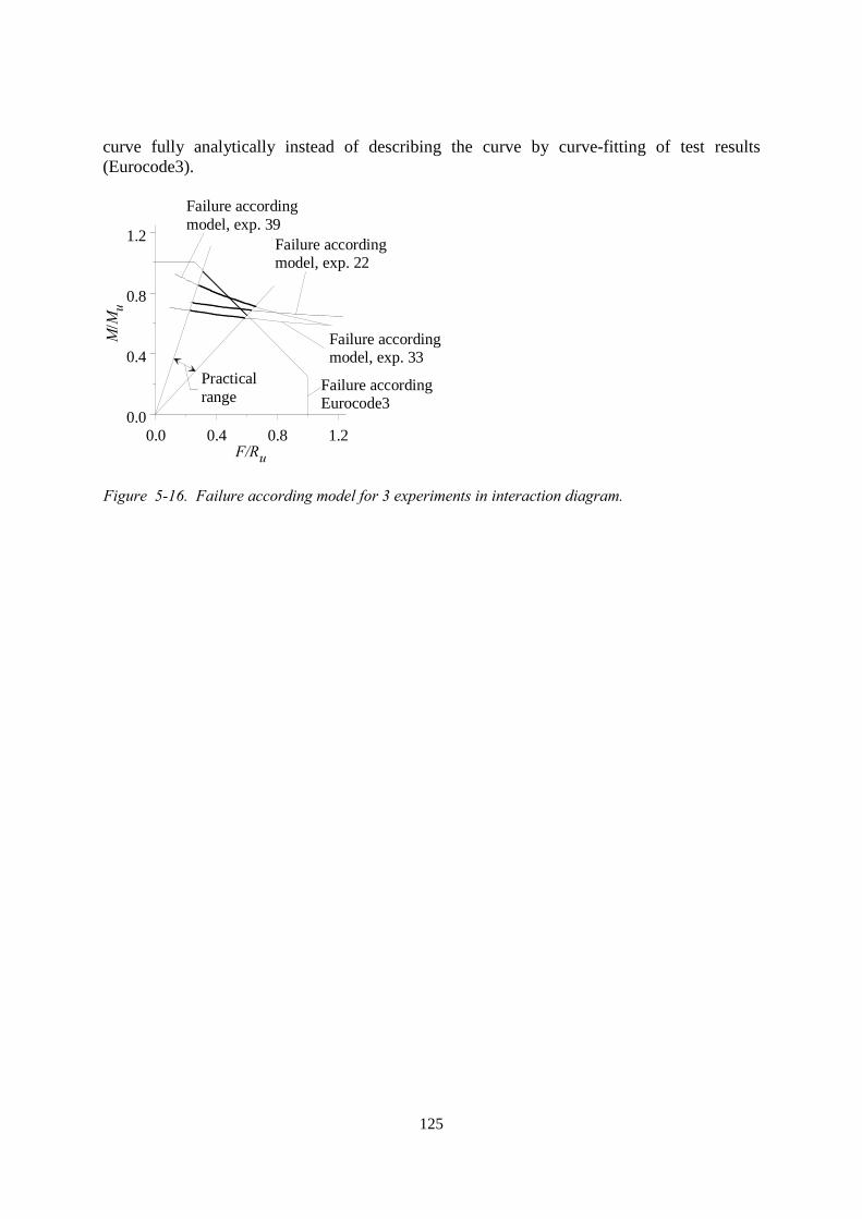
125
curve fully analytically instead of describing the curve by curve-fitting of test results(Eurocode3).
0.0 0.4 0.8 1.2F/Ru
0.0
0.4
0.8
1.2
M/ M
u
Failure accordingEurocode3
Failure accordingmodel, exp. 22
Failure accordingmodel, exp. 33
Failure accordingmodel, exp. 39
Practicalrange
Figure 5-16. Failure according model for 3 experiments in interaction diagram.

126
5.4 Conclusions
For the localised yield ultimate failure mode, a mechanical model was developed to predictthe failure of first-generation sheeting. In this model, the elastic cross-section deformations asa result of the concentrated load are determined first. Then, the cross-section deformations areused as an estimation of the imperfection of the bottom flange. This bottom flange is undercompression due to a bending moment in the sheeting. A solution of Marguerre's equations isthen used to determine the load for which the bottom flange (under compression and with animperfection) will start to yield.
Because the mechanical model is based on the structural behaviour of the sheeting, nointeraction rules are needed. The new model directly describes the relationship between theconcentrated load and bending moment.
All available experiments from literature are used to compare the mechanical model with thedesign rule of Eurocode3. For the correlation between predicted and experimental values, themechanical model performs equally to the Eurocode3 design rule. For the average ofpredicted divided by experimental values, the mechanical model gives too low a predictionfor the ultimate load. The average of Eurocode3 predictions is good, which is logical becauseEurocode3 is based on curve-fitting of test results. In conclusion, both the model andEurocode3 perform well.
The accuracy of the mechanical model and Eurocode3 was plotted for every variable. For theweb width, bottom flange width, corner radius, and angle between web and flange, there is norelationship between the accuracy of the models and the variables. For the other variables, themechanical model more often shows a relationship between accuracy and a variable than theEurocode3. This means there are more ways to improve the mechanical model than forEurocode3.

127
6 Post-failure modes
Chapter abstractWhy and when a specific post-failure mode occurs is investigated. In addition, the transitionis studied of one post-failure mode into another. All this is done by comparing theexperiments of chapter 3 with specific finite element models and post-failure mechanicalmodels. The post-failure mechanical models are introduced.
128
6.1 Introduction
In chapter 3, experiments were presented that showed that after ultimate load, three post-failure modes can occur for sheet sections: the rolling, the yield arc, and the yield eye post-failure modes.
In chapter 5, an ultimate failure mechanical model was presented that predicts the ultimateload for the localised yield ultimate failure mode (occurring for the yield arc and yield eyepost-failure modes). It was also explained that the rolling post-failure mode does not occur inpractice. Thus, the mechanical model is suitable for all situations in practice.
However, to use the mechanical model of chapter 5 properly, it still is important to knowunder which conditions a certain post-failure mode occurs or how one post-failure mode turnsinto an other. Besides this, for future research it may be important to not only have knowledgeabout the behaviour until and at ultimate load (the ultimate failure modes), but also afterultimate load (the post-failure modes).
Therefore, in this chapter the three post-failure modes are studied. This is done in a separatesection for each sheet section variable. Experiments of chapter 3, specific finite elementmodels, and post-failure mechanical models (to be introduced in sections 6.2 to 6.4) are usedto study the post-failure modes in sections 6.5 to 6.12. The way this study was carried out isexplained in sections 6.1.1 to 6.1.3.
6.1.1 Experiments chapter 3
Table 3-7 in chapter 3 presented the post-failure mode for each experiment. In this chapter,table 3-7 is used to find a possible relationship between a changing sheet section variable andthe occurring post-failure mode. Therefore, table 3-7 was scanned for sheet sections withexactly the same nominal value for all variables except the variable under investigation. As anexample, table 6-1 presents the old table 3-7, but now only with experiments shown that aredifferent for their span length.
6.1.2 Specific finite element models
Chapter 4 presented three finite element models, one for each post-failure mode. In section4.4.1, a set of finite element simulations was introduced with different span lengths, makinguse of the three finite element models. This set of simulations will be used in this chapter tostudy the occurrence of post-failure modes for changing span length. For the study of post-failure modes for a changing corner radius, another type of finite element model was used. Inthis finite element model, a very small strip dx (in length direction) of the sheet section ismodelled (figure 6-1). In this way, only cross-section behaviour is studied. This study ispresented in a detailed way in Appendix 4, report [Hofm00b].
6.1.3 Post-failure mechanical models
Chapter 5 presented an ultimate failure mechanical model. This model describes thebehaviour of the sheet section until and at ultimate load. However, as chapter 3 experiments
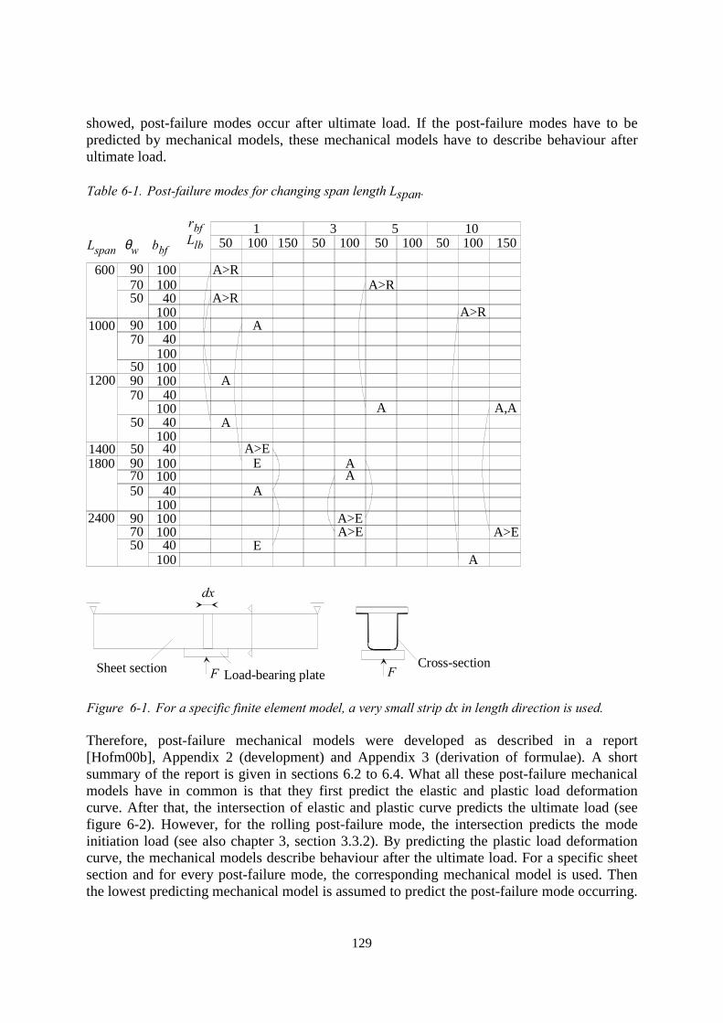
129
showed, post-failure modes occur after ultimate load. If the post-failure modes have to bepredicted by mechanical models, these mechanical models have to describe behaviour afterultimate load.
Table 6-1. Post-failure modes for changing span length Lspan.
Lspan θw bbf
rbfLlb 50 100 150
150 100
350 100
550 100 150
10
70
50
50
7090
50
1200
14001800
24007090
50
A100
10040
40100100
10040
10040
100100
A A,A
A
AA>E
AE
E
A>EA>E A>E
A
40
70 10090
50
600 A>R
A>RA>R
100
40100
A>R
5090
1000
100100
A
A
9070
100
10040
dx
FSheet section Load-bearing plate FCross-section
Figure 6-1. For a specific finite element model, a very small strip dx in length direction is used.
Therefore, post-failure mechanical models were developed as described in a report[Hofm00b], Appendix 2 (development) and Appendix 3 (derivation of formulae). A shortsummary of the report is given in sections 6.2 to 6.4. What all these post-failure mechanicalmodels have in common is that they first predict the elastic and plastic load deformationcurve. After that, the intersection of elastic and plastic curve predicts the ultimate load (seefigure 6-2). However, for the rolling post-failure mode, the intersection predicts the modeinitiation load (see also chapter 3, section 3.3.2). By predicting the plastic load deformationcurve, the mechanical models describe behaviour after the ultimate load. For a specific sheetsection and for every post-failure mode, the corresponding mechanical model is used. Thenthe lowest predicting mechanical model is assumed to predict the post-failure mode occurring.
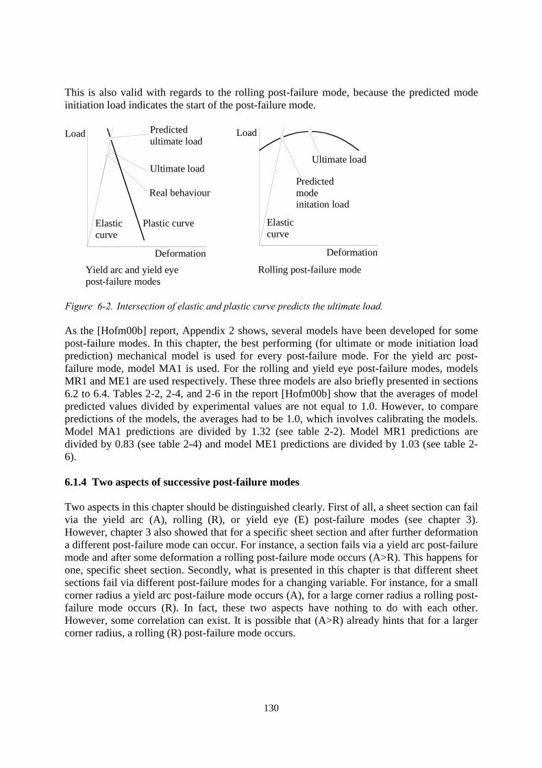
130
This is also valid with regards to the rolling post-failure mode, because the predicted modeinitiation load indicates the start of the post-failure mode.
Predictedultimate load
Real behaviour
Ultimate load
Load
Deformation
Elasticcurve
Plastic curve
Predictedmodeinitation load
Ultimate load
Load
Deformation
Elasticcurve
Yield arc and yield eye post-failure modes
Rolling post-failure mode
Figure 6-2. Intersection of elastic and plastic curve predicts the ultimate load.
As the [Hofm00b] report, Appendix 2 shows, several models have been developed for somepost-failure modes. In this chapter, the best performing (for ultimate or mode initiation loadprediction) mechanical model is used for every post-failure mode. For the yield arc post-failure mode, model MA1 is used. For the rolling and yield eye post-failure modes, modelsMR1 and ME1 are used respectively. These three models are also briefly presented in sections6.2 to 6.4. Tables 2-2, 2-4, and 2-6 in the report [Hofm00b] show that the averages of modelpredicted values divided by experimental values are not equal to 1.0. However, to comparepredictions of the models, the averages had to be 1.0, which involves calibrating the models.Model MA1 predictions are divided by 1.32 (see table 2-2). Model MR1 predictions aredivided by 0.83 (see table 2-4) and model ME1 predictions are divided by 1.03 (see table 2-6).
6.1.4 Two aspects of successive post-failure modes
Two aspects in this chapter should be distinguished clearly. First of all, a sheet section can failvia the yield arc (A), rolling (R), or yield eye (E) post-failure modes (see chapter 3).However, chapter 3 also showed that for a specific sheet section and after further deformationa different post-failure mode can occur. For instance, a section fails via a yield arc post-failuremode and after some deformation a rolling post-failure mode occurs (A>R). This happens forone, specific sheet section. Secondly, what is presented in this chapter is that different sheetsections fail via different post-failure modes for a changing variable. For instance, for a smallcorner radius a yield arc post-failure mode occurs (A), for a large corner radius a rolling post-failure mode occurs (R). In fact, these two aspects have nothing to do with each other.However, some correlation can exist. It is possible that (A>R) already hints that for a largercorner radius, a rolling (R) post-failure mode occurs.
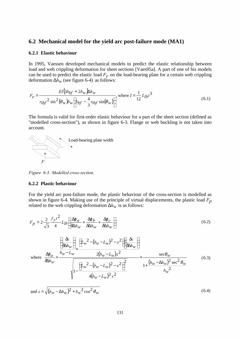
131
6.2 Mechanical model for the yield arc post-failure mode (MA1)
6.2.1 Elastic behaviour
In 1995, Vaessen developed mechanical models to predict the elastic relationship betweenload and web crippling deformation for sheet sections [Vaes95a]. A part of one of his modelscan be used to predict the elastic load Fe on the load-bearing plate for a certain web cripplingdeformation ∆hw (see figure 6-4) as follows:
( )( ) ( )
3121 where,
sin342sin2
23tlbLI
wibfrbfbwbwibfr
whwbbfbEIeF =
−
∆+=
θθ(6.1)
The formula is valid for first-order elastic behaviour for a part of the sheet section (defined as"modelled cross-section"), as shown in figure 6-3. Flange or web buckling is not taken intoaccount.
F
Load-bearing plate width
Figure 6-3. Modelled cross-section.
6.2.2 Plastic behaviour
For the yield arc post-failure mode, the plastic behaviour of the cross-section is modelled asshown in figure 6-4. Making use of the principle of virtual displacements, the plastic load Fprelated to the web crippling deformation ∆hw is as follows:
∆
+∆
+∆
=whc
whb
wha
lbLtyf
pFδδϕ
δδϕ
δδϕ
4
2
322 (6.2)
( )
( )
( )
( )
( )
2
2sec21
sec
224
2222
1
22
222
where
wbwwhwh
w
xwLwb
xwLwbwL
xwLwb
whxxwLwbwL
wLwbwh
x
wha
θ
θ
δδ
δδ
δδϕ
∆−+
+
−
−−−−
−
∆
−−−
+−
∆
=∆
(6.3)
( ) wwbwhwhx θ2cos22 and +∆−= (6.4)
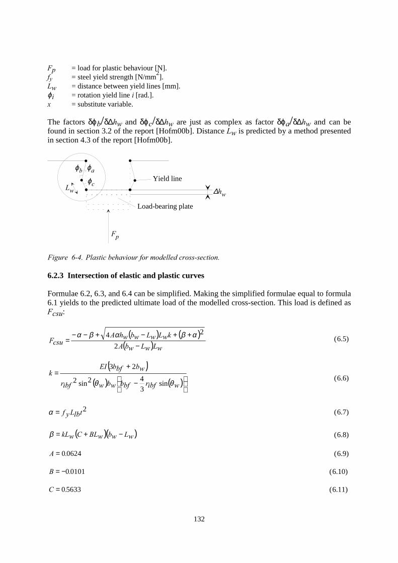
132
Fp = load for plastic behaviour [N].fy = steel yield strength [N/mm2].Lw = distance between yield lines [mm].ϕi = rotation yield line i [rad.].x = substitute variable.
The factors δϕb/δ∆hw and δϕc/δ∆hw are just as complex as factor δϕa/δ∆hw and can befound in section 3.2 of the report [Hofm00b]. Distance Lw is predicted by a method presentedin section 4.3 of the report [Hofm00b].
Load-bearing plate
Yield line
Fp
∆hw
ϕaϕb
ϕcLw
Figure 6-4. Plastic behaviour for modelled cross-section.
6.2.3 Intersection of elastic and plastic curves
Formulae 6.2, 6.3, and 6.4 can be simplified. Making the simplified formulae equal to formula6.1 yields to the predicted ultimate load of the modelled cross-section. This load is defined asFcsu:
( ) ( )( ) wLwLwbA
kwLwLwbwhAcsuF
−++−+−−
=2
24 αβαβα (6.5)
( )( ) ( )
sin
342sin2
23
−
+=
wibfrbfbwbwibfr
wbbfbEIk
θθ(6.6)
2tlbLyf=α (6.7)
( )( ) wLwbwBLCwkL −+=β (6.8)
06240.A = (6.9)
01010.B −= (6.10)
56330.C = (6.11)
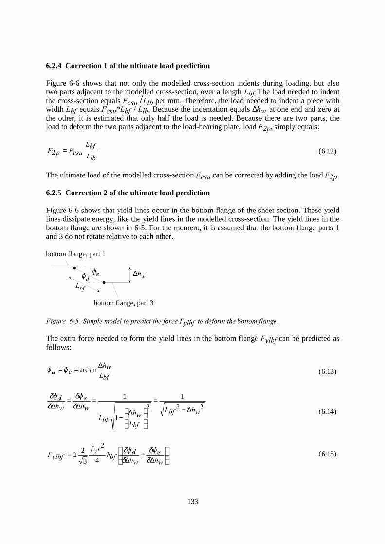
133
6.2.4 Correction 1 of the ultimate load prediction
Figure 6-6 shows that not only the modelled cross-section indents during loading, but alsotwo parts adjacent to the modelled cross-section, over a length Lbf. The load needed to indentthe cross-section equals Fcsu /Llb per mm. Therefore, the load needed to indent a piece withwidth Lbf equals Fcsu*Lbf / Llb. Because the indentation equals ∆hw at one end and zero atthe other, it is estimated that only half the load is needed. Because there are two parts, theload to deform the two parts adjacent to the load-bearing plate, load F2p, simply equals:
lbLbfL
csuFpF =2 (6.12)
The ultimate load of the modelled cross-section Fcsu can be corrected by adding the load F2p.
6.2.5 Correction 2 of the ultimate load prediction
Figure 6-6 shows that yield lines occur in the bottom flange of the sheet section. These yieldlines dissipate energy, like the yield lines in the modelled cross-section. The yield lines in thebottom flange are shown in 6-5. For the moment, it is assumed that the bottom flange parts 1and 3 do not rotate relative to each other.
Lbf
∆hwϕdϕe
bottom flange, part 1
bottom flange, part 3
Figure 6-5. Simple model to predict the force Fylbf to deform the bottom flange.
The extra force needed to form the yield lines in the bottom flange Fylbf can be predicted asfollows:
bfLwh
ed∆
== arcsinϕϕ (6.13)
221
21
1
whbfL
bfLwh
bfLwhe
whd
∆−=
∆−
=∆
=∆ δ
δϕδδϕ
(6.14)
∆
+∆
=whe
whd
bfbtyf
ylbfFδδϕ
δδϕ
4
2
322 (6.15)
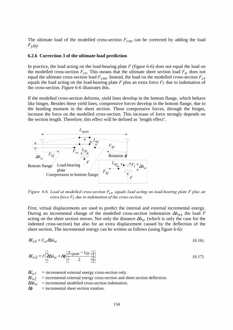
134
The ultimate load of the modelled cross-section Fcsu can be corrected by adding the loadFylbf.
6.2.6 Correction 3 of the ultimate load prediction
In practice, the load acting on the load-bearing plate F (figure 6-6) does not equal the load onthe modelled cross-section Fcs. This means that the ultimate sheet section load Fu does notequal the ultimate cross-section load Fcsu. Instead, the load on the modelled cross-section Fcsequals the load acting on the load-bearing plate F plus an extra force Fl due to indentation ofthe cross-section. Figure 6-6 illustrates this.
If the modelled cross-section deforms, yield lines develop in the bottom flange, which behavelike hinges. Besides these yield lines, compressive forces develop in the bottom flange, due tothe bending moment in the sheet section. These compressive forces, through the hinges,increase the force on the modelled cross-section. This increase of force strongly depends onthe section length. Therefore, this effect will be defined as ‘length effect’.
Load-bearingplate
Rotation ϕ
Bottom flange
Compression in bottom flange
F
F
Lspan
FlFbf
Lbf ∆hw
LbfFbf
∆hwFbf
FcsLlb
Figure 6-6. Load at modelled cross-section Fcs equals load acting on load-bearing plate F plus anextra force Fl due to indentation of the cross-section.
First, virtual displacements are used to predict the internal and external incremental energy.During an incremental change of the modelled cross-section indentation ∆hw, the load Facting on the sheet section moves. Not only the distance ∆hw (which is only the case for theindented cross-section) but also for an extra displacement caused by the deflection of thesheet section. The incremental energy can be written as follows (using figure 6-6):
whcsFeE ∆= δδ 1 (6.16)
−+∆=
22lbLspanL
whFeE δϕδδ (6.17)
δEe1 = incremental external energy cross-section only.δEe2 = incremental external energy cross-section and sheet section deflection.δ∆hw = incremental modelled cross-section indentation.δϕ = incremental sheet section rotation.
135
Influences of stress on yield line energy dissipation are neglected and it is assumed that theyield line pattern does not change geometrically during deformation. Then, because bothmentioned external energy terms should equal the incremental internal energy and internalenergy is equal for both cases, we can derive the following:
⇔= 21 eEeE δδ
⇔
−+∆
∆=⇔
−+∆=∆
2
2 lbLspanLwh
whcsFFlbLspanL
whFwhcsF
δϕδ
δδϕδδ
1*
21
1lfcsF
lbLspanL
wh
csFF =
−
∆+
=
δδϕ (6.18)
fl1 = length factor 1
The factor δϕ/δ∆hw is complex and can only be predicted with complicated formulae (report[Hofm00b], Appendix 3, section 3.3). The ultimate load of the modelled cross-section Fcsu iscorrected by multiplying the load with factor fl1.
6.2.7 Ultimate load Fu
The ultimate load is now found as follows:
( ) 12 lfylbfFpFcsuFuF ++= (6.19)
6.2.8 Yield line distance Lbf
The distance between yield lines Lbf is shown in figure 6-6. The distance Lbf can bedetermined by varying Lbf and finding the minimum value for the ultimate load Fu:
csuFbfblbLtyf
bfL4
601.222= (6.20)
6.2.9 Summary
The ultimate load of a sheet section for the yield arc post-failure mode is predicted by modelMA1 as follows:
1. Yield line distance Lw is predicted by a mechanical model presented in section 4.3 of thereport [Hofm00b].

136
2. The ultimate load for the modelled cross-section Fcsu is determined using formulae 6.5 to6.11.
3. Distance Lbf is predicted by formula 6.20.
4. Load F2p is predicted by formula 6.12 and added to load Fcsu.
5. Load Fylbf is predicted by formulae 6.13 to 6.15 and added to load Fcsu.
6. Factor fl1 is calculated by formula 6.18.
7. Load Fu is found by formula 6.19.
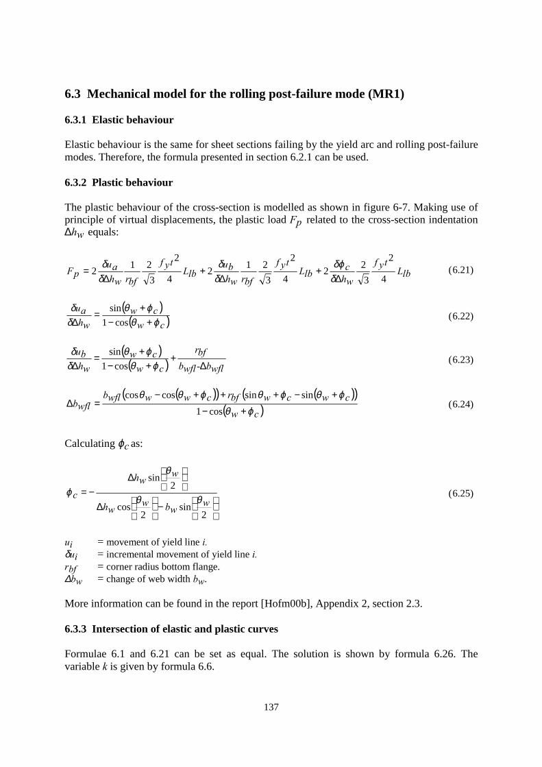
137
6.3 Mechanical model for the rolling post-failure mode (MR1)
6.3.1 Elastic behaviour
Elastic behaviour is the same for sheet sections failing by the yield arc and rolling post-failuremodes. Therefore, the formula presented in section 6.2.1 can be used.
6.3.2 Plastic behaviour
The plastic behaviour of the cross-section is modelled as shown in figure 6-7. Making use ofprinciple of virtual displacements, the plastic load Fp related to the cross-section indentation∆hw equals:
lbLtyf
whc
lbLtyf
bfrwhbu
lbLtyf
bfrwhau
pF4
2
322
4
2
3212
4
2
3212
∆+
∆+
∆=
δδϕ
δδ
δδ (6.21)
( )( ) cos1
sin
cwcw
whau
ϕθϕθ
δδ
+−+
=∆ (6.22)
( )( ) wflb-wflb
bfr
cwcw
whbu
∆+
+−+
=∆ ϕθ
ϕθδδ
cos1sin
(6.23)
( )( ) ( )( )( )cw
cwcwbfrcwwwflbwflb
ϕθϕθϕθϕθθ
+−
+−+++−=∆
cos1sinsincoscos
(6.24)
Calculating ϕc as:
−
∆
∆
−=
2sin
2cos
2sin
wwbw
wh
wwh
c θθ
θ
ϕ (6.25)
ui = movement of yield line i.δui = incremental movement of yield line i.rbf = corner radius bottom flange.∆bw = change of web width bw.
More information can be found in the report [Hofm00b], Appendix 2, section 2.3.
6.3.3 Intersection of elastic and plastic curves
Formulae 6.1 and 6.21 can be set as equal. The solution is shown by formula 6.26. Thevariable k is given by formula 6.6.
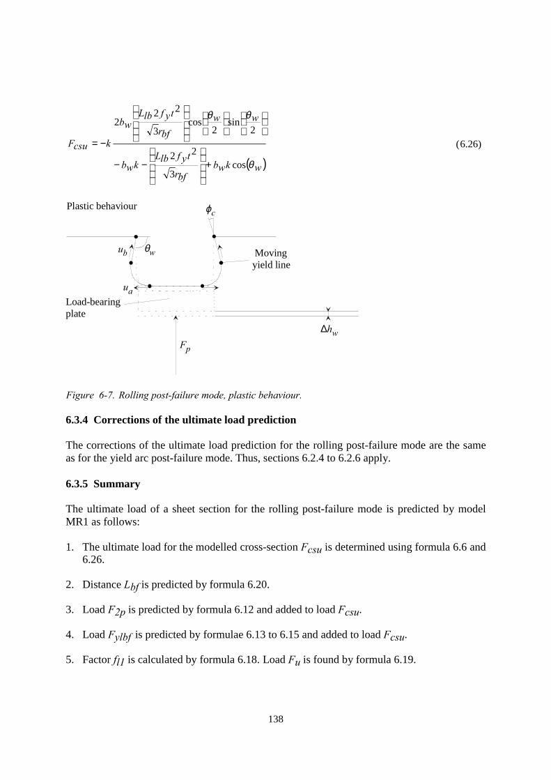
138
( )
cos3
22
2sin
2cos
3
222
wkwbbfr
tyflbLkwb
wwbfr
tyflbLwb
kcsuF
θ
θθ
+
−−
−= (6.26)
Load-bearingplate
Plastic behaviour
Movingyield line
∆hwFp
ua
ub θw
ϕc
Figure 6-7. Rolling post-failure mode, plastic behaviour.
6.3.4 Corrections of the ultimate load prediction
The corrections of the ultimate load prediction for the rolling post-failure mode are the sameas for the yield arc post-failure mode. Thus, sections 6.2.4 to 6.2.6 apply.
6.3.5 Summary
The ultimate load of a sheet section for the rolling post-failure mode is predicted by modelMR1 as follows:
1. The ultimate load for the modelled cross-section Fcsu is determined using formula 6.6 and6.26.
2. Distance Lbf is predicted by formula 6.20.
3. Load F2p is predicted by formula 6.12 and added to load Fcsu.
4. Load Fylbf is predicted by formulae 6.13 to 6.15 and added to load Fcsu.
5. Factor fl1 is calculated by formula 6.18. Load Fu is found by formula 6.19.
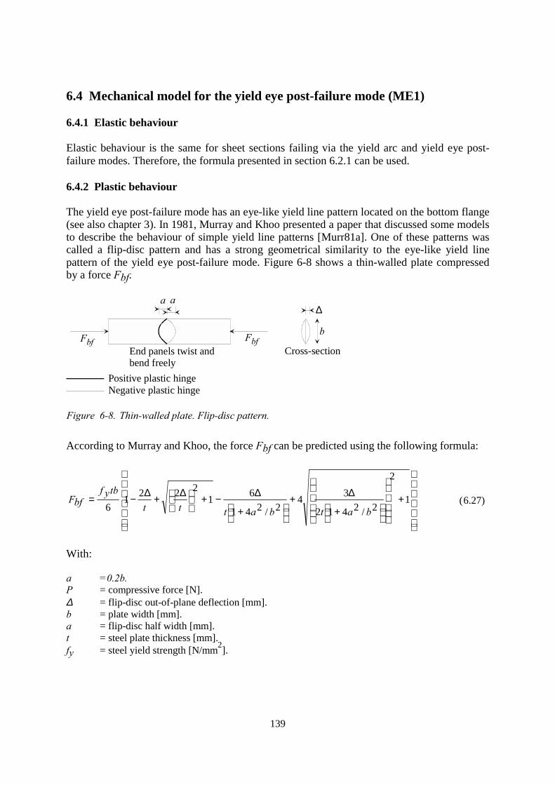
139
6.4 Mechanical model for the yield eye post-failure mode (ME1)
6.4.1 Elastic behaviour
Elastic behaviour is the same for sheet sections failing via the yield arc and yield eye post-failure modes. Therefore, the formula presented in section 6.2.1 can be used.
6.4.2 Plastic behaviour
The yield eye post-failure mode has an eye-like yield line pattern located on the bottom flange(see also chapter 3). In 1981, Murray and Khoo presented a paper that discussed some modelsto describe the behaviour of simple yield line patterns [Murr81a]. One of these patterns wascalled a flip-disc pattern and has a strong geometrical similarity to the eye-like yield linepattern of the yield eye post-failure mode. Figure 6-8 shows a thin-walled plate compressedby a force Fbf.
Fbf
aa
End panels twist and bend freely
Positive plastic hingeNegative plastic hinge
∆
Cross-section
bFbf
Figure 6-8. Thin-walled plate. Flip-disc pattern.
According to Murray and Khoo, the force Fbf can be predicted using the following formula:
1
2
2/2412
342/241
612221
6
+
+
∆+
+
∆−+
∆+∆−=
batbattt
tbyfbfF (6.27)
With:
a =0.2b.P = compressive force [N].∆ = flip-disc out-of-plane deflection [mm].b = plate width [mm].a = flip-disc half width [mm].t = steel plate thickness [mm].fy = steel yield strength [N/mm2].
140
6.4.3 Intersection of elastic and plastic curves
Formula 6.1 describes the relationship between the concentrated load F acting on the sheetsection and the sheet section web crippling deformation ∆hw. Formula 6.27 defines the loadFbf acting on the bottom flange needed to form a plastic mechanism for a certain flip-disc out-of-plane deflection ∆ (previous section). Thus, elastic and plastic curves have different loadand deformation variables. A relationship between the load on the sheet section F and the loadon the bottom flange Fbf should develop. Furthermore a relationship between the elasticcross-section deformation variable ∆hw and the plastic flip-disc deformation variable∆ should develop.
6.4.4 Cross-section deformation versus flip-disc deformation
Figure 6-9 shows a possible relationship for this: for elastic behaviour, it is assumed that acertain width adjacent to the modelled cross-section will deform like the modelled cross-section. This certain width is set equal to the distance 2a between yield lines in the bottomflange during plastic deformation. This leads to the following derivation:
whawh
a∆=∆⇔
∆=∆ 5.0
222 (6.28)
∆ = flip-disc out-of-plane deflection [mm].∆hw = web crippling deformation [mm].
6.4.5 Load at section versus load at bottom flange
Looking at figure 6-9 we see that the external bending moment in the section equals:
4spanFL
eM = (6.29)
Me = external bending moment [Nmm]F = concentrated load of support on section [N]Lspan = span length [mm]
This gives the following assumptions:
• One concentrated load F models the load of the load-bearing plate.
• The flip-disc occurs in the position of this concentrated load, i.e. the location of highestbending moment.
The internal bending moment in the section equals:
tsbfbsIbfF
iMssIiM
tbfbbfF
*=⇔= (6.30)
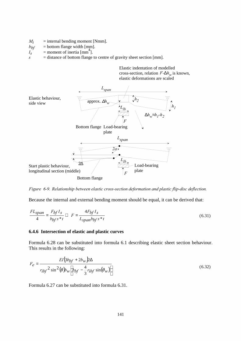
141
Mi = internal bending moment [Nmm].bbf = bottom flange width [mm].Is = moment of inertia [mm4].s = distance of bottom flange to centre of gravity sheet section [mm].
∆hw=h1-h2
Bottom flangeF
Lspan
Llb
Elastic indentation of modelledcross-section, relation is known,elastic deformations are scaled
2∆
Bottom flangeF
2a
Elastic behaviour,side view
Start plastic behaviour,longitudinal section (middle)
h1
h2approx. ∆hw
Llb
Lspan
Load-bearingplate
Load-bearingplate
F-∆hw
Figure 6-9. Relationship between elastic cross-section deformation and plastic flip-disc deflection.
Because the internal and external bending moment should be equal, it can be derived that:
tsbfbspanLsIbfF
Ftsbfb
sIbfFspanFL*
4*4
=⇔= (6.31)
6.4.6 Intersection of elastic and plastic curves
Formula 6.28 can be substituted into formula 6.1 describing elastic sheet section behaviour.This results in the following:
( )( ) ( )
−
∆+=
wibfrbfbwbibfr
wbbfbEIeF
θθ sin342sin2
223(6.32)
Formula 6.27 can be substituted into formula 6.31.
142
This results in:
1
2
2/2412
342/241
612221
6
**
4
+
+
∆+
+
∆−+
∆+∆−
=
batbattt
tbyf
tsbfbspanLsIbfF
pF
(6.33)
If the elastic load Fe and the plastic load Fp are set as equal, the flip-disc out-of-planedisplacement can be solved. Then the ultimate sheet section load Fu can be calculated byusing the value for ∆ into formulae 6.32 or 6.33.
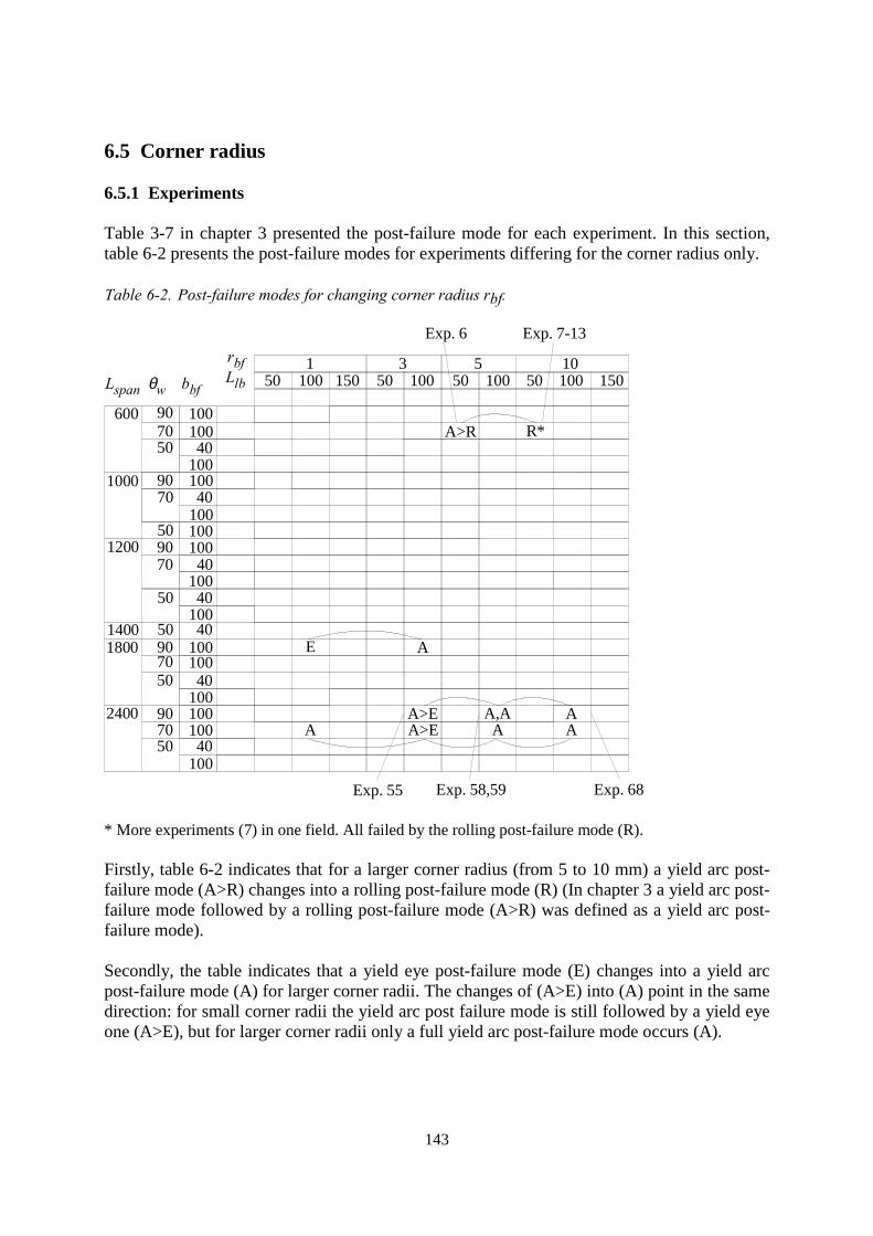
143
6.5 Corner radius
6.5.1 Experiments
Table 3-7 in chapter 3 presented the post-failure mode for each experiment. In this section,table 6-2 presents the post-failure modes for experiments differing for the corner radius only.
Table 6-2. Post-failure modes for changing corner radius rbf.
Lspan θw bbf
rbfLlb 50 100 150
150 100
350 100
550 100 150
10
70
50
50
7090
50
1200
14001800
24007090
50
100
10040
40100100
10040
10040
100100
AE
AA>EA>E
A,AA
AA
40
70 10090
50
600R*
100
40100
A>R
5090
1000
100100
9070
100
10040
Exp. 6 Exp. 7-13
Exp. 55 Exp. 58,59 Exp. 68
* More experiments (7) in one field. All failed by the rolling post-failure mode (R).
Firstly, table 6-2 indicates that for a larger corner radius (from 5 to 10 mm) a yield arc post-failure mode (A>R) changes into a rolling post-failure mode (R) (In chapter 3 a yield arc post-failure mode followed by a rolling post-failure mode (A>R) was defined as a yield arc post-failure mode).
Secondly, the table indicates that a yield eye post-failure mode (E) changes into a yield arcpost-failure mode (A) for larger corner radii. The changes of (A>E) into (A) point in the samedirection: for small corner radii the yield arc post failure mode is still followed by a yield eyeone (A>E), but for larger corner radii only a full yield arc post-failure mode occurs (A).
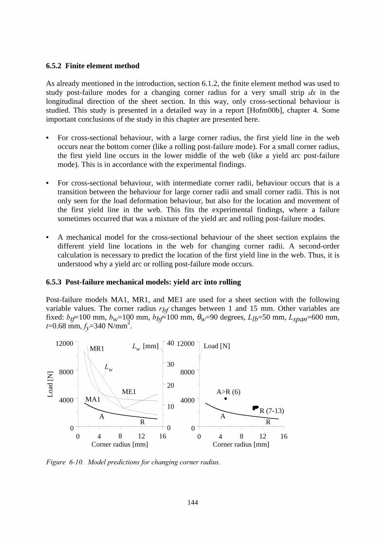
144
6.5.2 Finite element method
As already mentioned in the introduction, section 6.1.2, the finite element method was used tostudy post-failure modes for a changing corner radius for a very small strip dx in thelongitudinal direction of the sheet section. In this way, only cross-sectional behaviour isstudied. This study is presented in a detailed way in a report [Hofm00b], chapter 4. Someimportant conclusions of the study in this chapter are presented here.
• For cross-sectional behaviour, with a large corner radius, the first yield line in the weboccurs near the bottom corner (like a rolling post-failure mode). For a small corner radius,the first yield line occurs in the lower middle of the web (like a yield arc post-failuremode). This is in accordance with the experimental findings.
• For cross-sectional behaviour, with intermediate corner radii, behaviour occurs that is atransition between the behaviour for large corner radii and small corner radii. This is notonly seen for the load deformation behaviour, but also for the location and movement ofthe first yield line in the web. This fits the experimental findings, where a failuresometimes occurred that was a mixture of the yield arc and rolling post-failure modes.
• A mechanical model for the cross-sectional behaviour of the sheet section explains thedifferent yield line locations in the web for changing corner radii. A second-ordercalculation is necessary to predict the location of the first yield line in the web. Thus, it isunderstood why a yield arc or rolling post-failure mode occurs.
6.5.3 Post-failure mechanical models: yield arc into rolling
Post-failure models MA1, MR1, and ME1 are used for a sheet section with the followingvariable values. The corner radius rbf changes between 1 and 15 mm. Other variables arefixed: btf=100 mm, bw=100 mm, bbf=100 mm, θw=90 degrees, Llb=50 mm, Lspan=600 mm,t=0.68 mm, fy=340 N/mm2.
0 4 8 12 16Corner radius [mm]
0
4000
8000
12000
Load
[N]
0 4 8 12 16Corner radius [mm]
0
4000
8000
12000
R (7-13)
A>R (6)ME1MA1
MR1
AR
AR
0
10
20
30
40
Lw
Lw [mm] Load [N]
Figure 6-10. Model predictions for changing corner radius.
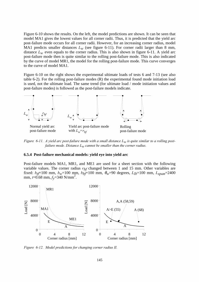
145
Figure 6-10 shows the results. On the left, the model predictions are shown. It can be seen thatmodel MA1 gives the lowest values for all corner radii. Thus, it is predicted that the yield arcpost-failure mode occurs for all corner radii. However, for an increasing corner radius, modelMA1 predicts smaller distances Lw (see figure 6-11). For corner radii larger than 8 mm,distance Lw even equals to the corner radius. This is also shown in figure 6-11. A yield arcpost-failure mode then is quite similar to the rolling post-failure mode. This is also indicatedby the curve of model MR1, the model for the rolling post-failure mode. This curve convergesto the curve of model MA1.
Figure 6-10 on the right shows the experimental ultimate loads of tests 6 and 7-13 (see alsotable 6-2). For the rolling post-failure modes (R) the experimental found mode initiation loadis used, not the ultimate load. The same trend (for ultimate load / mode initiation values andpost-failure modes) is followed as the post-failure models indicate.
Lw rbf
Normal yield arcpost-failure mode
Lw
Yield arc post-failure modewith Lw=rbf
Rollingpost-failure mode
Figure 6-11. A yield arc post-failure mode with a small distance Lw is quite similar to a rolling post-failure mode. Distance Lw cannot be smaller than the corner radius.
6.5.4 Post-failure mechanical models: yield eye into yield arc
Post-failure models MA1, MR1, and ME1 are used for a sheet section with the followingvariable values. The corner radius rbf changed between 1 and 15 mm. Other variables arefixed: btf=100 mm, bw=100 mm, bbf=100 mm, θw=90 degrees, Llb=100 mm, Lspan=2400mm, t=0.68 mm, fy=340 N/mm2.
0 4 8 12Corner radius [mm]
0
4000
8000
12000
0 4 8 12Corner radius [mm]
0
4000
8000
12000
Load
[N]
Load
[N]
EA
MR1
ME1
MA1
EA
A (68)
A,A (58,59)
A>E (55)
Figure 6-12. Model predictions for changing corner radius II.
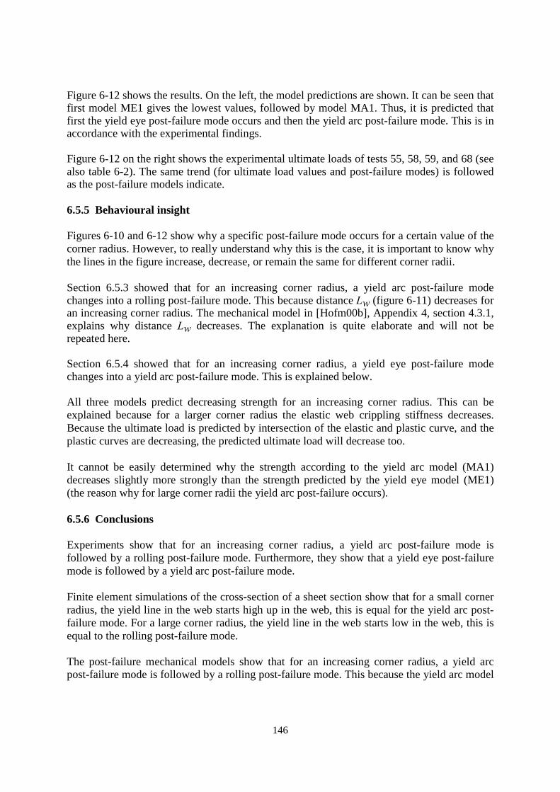
146
Figure 6-12 shows the results. On the left, the model predictions are shown. It can be seen thatfirst model ME1 gives the lowest values, followed by model MA1. Thus, it is predicted thatfirst the yield eye post-failure mode occurs and then the yield arc post-failure mode. This is inaccordance with the experimental findings.
Figure 6-12 on the right shows the experimental ultimate loads of tests 55, 58, 59, and 68 (seealso table 6-2). The same trend (for ultimate load values and post-failure modes) is followedas the post-failure models indicate.
6.5.5 Behavioural insight
Figures 6-10 and 6-12 show why a specific post-failure mode occurs for a certain value of thecorner radius. However, to really understand why this is the case, it is important to know whythe lines in the figure increase, decrease, or remain the same for different corner radii.
Section 6.5.3 showed that for an increasing corner radius, a yield arc post-failure modechanges into a rolling post-failure mode. This because distance Lw (figure 6-11) decreases foran increasing corner radius. The mechanical model in [Hofm00b], Appendix 4, section 4.3.1,explains why distance Lw decreases. The explanation is quite elaborate and will not berepeated here.
Section 6.5.4 showed that for an increasing corner radius, a yield eye post-failure modechanges into a yield arc post-failure mode. This is explained below.
All three models predict decreasing strength for an increasing corner radius. This can beexplained because for a larger corner radius the elastic web crippling stiffness decreases.Because the ultimate load is predicted by intersection of the elastic and plastic curve, and theplastic curves are decreasing, the predicted ultimate load will decrease too.
It cannot be easily determined why the strength according to the yield arc model (MA1)decreases slightly more strongly than the strength predicted by the yield eye model (ME1)(the reason why for large corner radii the yield arc post-failure occurs).
6.5.6 Conclusions
Experiments show that for an increasing corner radius, a yield arc post-failure mode isfollowed by a rolling post-failure mode. Furthermore, they show that a yield eye post-failuremode is followed by a yield arc post-failure mode.
Finite element simulations of the cross-section of a sheet section show that for a small cornerradius, the yield line in the web starts high up in the web, this is equal for the yield arc post-failure mode. For a large corner radius, the yield line in the web starts low in the web, this isequal to the rolling post-failure mode.
The post-failure mechanical models show that for an increasing corner radius, a yield arcpost-failure mode is followed by a rolling post-failure mode. This because the yield arc model

147
predicts a lower distance Lw. Why this model predicts a lower distance Lw is explained in[Hofm00b], Appendix 4, section 4.3.1.
The post-failure mechanical models show that for an increasing corner radius, a yield eyepost-failure mode is followed by a yield arc post-failure mode.
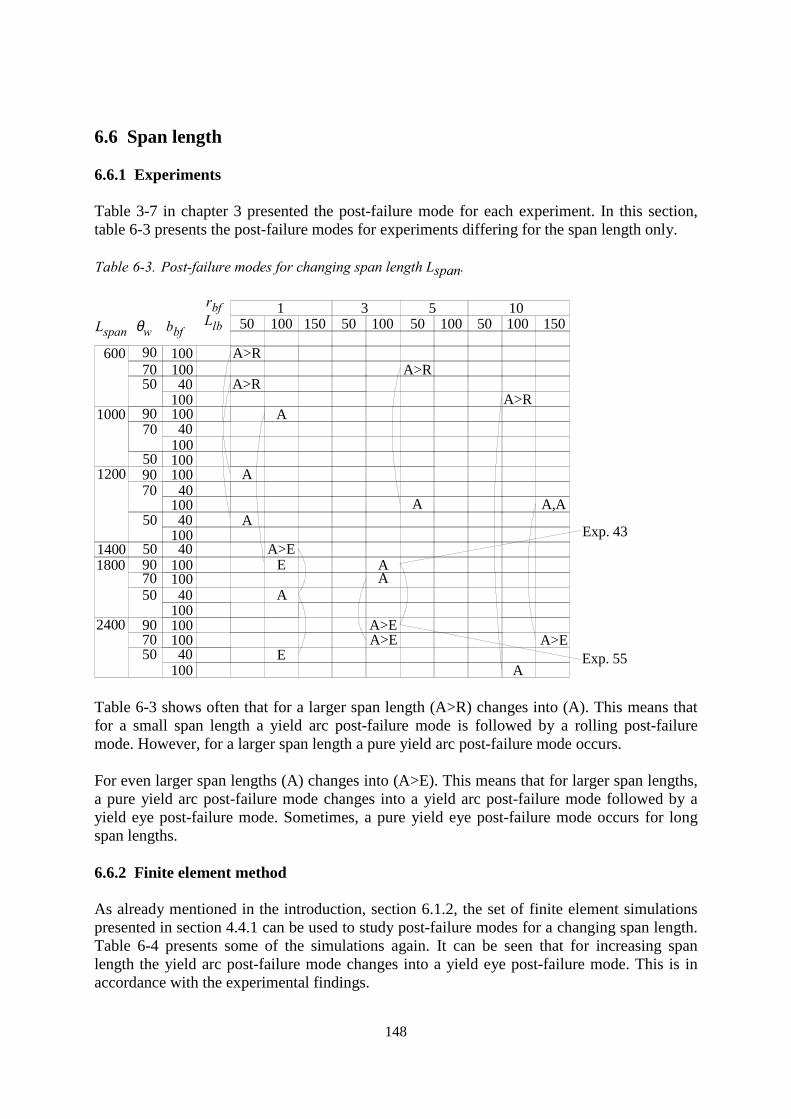
148
6.6 Span length
6.6.1 Experiments
Table 3-7 in chapter 3 presented the post-failure mode for each experiment. In this section,table 6-3 presents the post-failure modes for experiments differing for the span length only.
Table 6-3. Post-failure modes for changing span length Lspan.
Lspan θw bbf
rbfLlb 50 100 150
150 100
350 100
550 100 150
10
70
50
50
7090
50
1200
14001800
24007090
50
A100
10040
40100100
10040
10040
100100
A A,A
A
AA>E
AE
E
A>EA>E A>E
A
40
70 10090
50
600 A>R
A>RA>R
100
40100
A>R
5090
1000
100100
A
A
9070
100
10040
Exp. 43
Exp. 55
Table 6-3 shows often that for a larger span length (A>R) changes into (A). This means thatfor a small span length a yield arc post-failure mode is followed by a rolling post-failuremode. However, for a larger span length a pure yield arc post-failure mode occurs.
For even larger span lengths (A) changes into (A>E). This means that for larger span lengths,a pure yield arc post-failure mode changes into a yield arc post-failure mode followed by ayield eye post-failure mode. Sometimes, a pure yield eye post-failure mode occurs for longspan lengths.
6.6.2 Finite element method
As already mentioned in the introduction, section 6.1.2, the set of finite element simulationspresented in section 4.4.1 can be used to study post-failure modes for a changing span length.Table 6-4 presents some of the simulations again. It can be seen that for increasing spanlength the yield arc post-failure mode changes into a yield eye post-failure mode. This is inaccordance with the experimental findings.
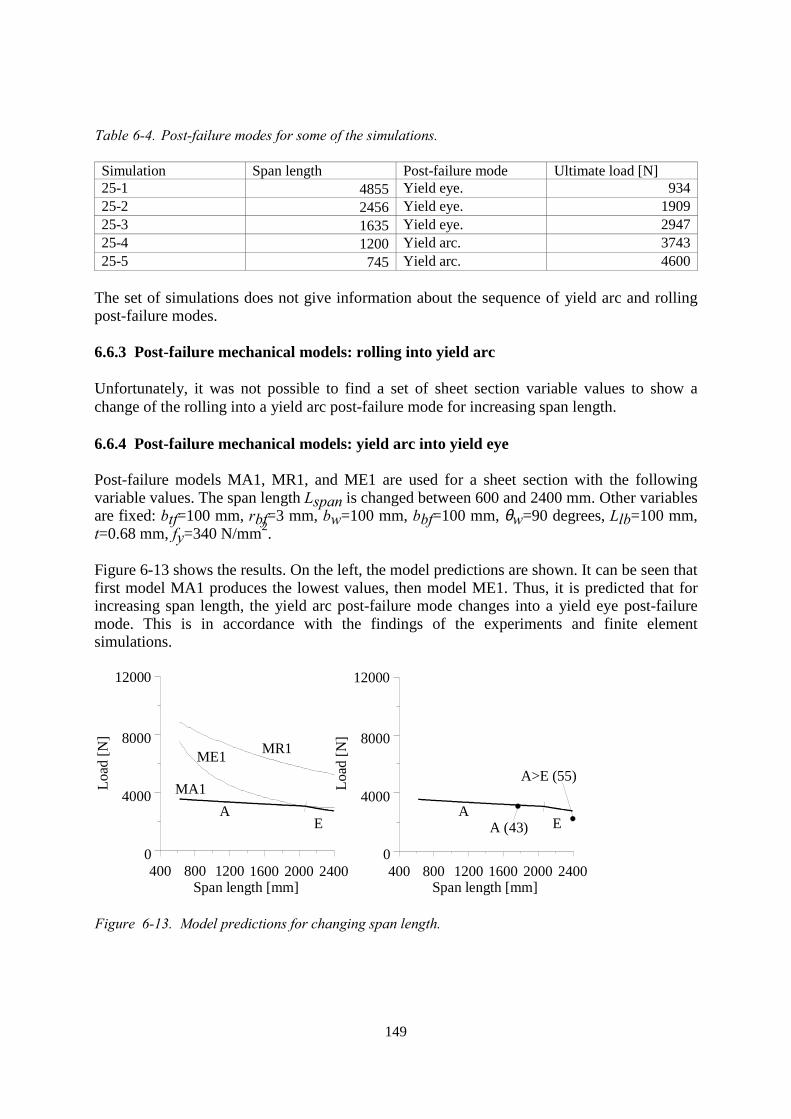
149
Table 6-4. Post-failure modes for some of the simulations.
Simulation Span length Post-failure mode Ultimate load [N]25-1 4855 Yield eye. 93425-2 2456 Yield eye. 190925-3 1635 Yield eye. 294725-4 1200 Yield arc. 374325-5 745 Yield arc. 4600
The set of simulations does not give information about the sequence of yield arc and rollingpost-failure modes.
6.6.3 Post-failure mechanical models: rolling into yield arc
Unfortunately, it was not possible to find a set of sheet section variable values to show achange of the rolling into a yield arc post-failure mode for increasing span length.
6.6.4 Post-failure mechanical models: yield arc into yield eye
Post-failure models MA1, MR1, and ME1 are used for a sheet section with the followingvariable values. The span length Lspan is changed between 600 and 2400 mm. Other variablesare fixed: btf=100 mm, rbf=3 mm, bw=100 mm, bbf=100 mm, θw=90 degrees, Llb=100 mm,t=0.68 mm, fy=340 N/mm2.
Figure 6-13 shows the results. On the left, the model predictions are shown. It can be seen thatfirst model MA1 produces the lowest values, then model ME1. Thus, it is predicted that forincreasing span length, the yield arc post-failure mode changes into a yield eye post-failuremode. This is in accordance with the findings of the experiments and finite elementsimulations.
400 800 1200 1600 2000 2400Span length [mm]
0
4000
8000
12000
AE
400 800 1200 1600 2000 2400Span length [mm]
0
4000
8000
12000
AE
Load
[N]
Load
[N]
MA1
MR1ME1
A (43)
A>E (55)
Figure 6-13. Model predictions for changing span length.

150
Figure 6-13 on the right shows the experimental ultimate loads of tests 43 and 55 (see alsotable 6-3). The same trend for ultimate load values and post-failure modes is observed as thepost-failure models indicate.
6.6.5 Behavioural insight
For long span lengths, the stresses in the bottom flange increase strongly. Therefore theplastic load for the yield eye model (ME1) is reached more easily. Although the rolling andyield arc post-failure mechanical models decrease in strength (due to the length factor), thiseffect is not as strong as the influence of increasing stress for the yield eye model.
6.6.6 Conclusions
Experiments show that for an increasing span length, a yield arc post-failure mode is followedby a yield eye post-failure mode. Furthermore, they suggest that a rolling post-failure mode isfollowed by a yield arc post failure mode.
Finite element simulations show that for an increasing span length, a yield arc post-failuremode is followed by a yield eye post-failure mode. The post-failure mechanical models showresults in accordance with the experiments and finite element simulations.
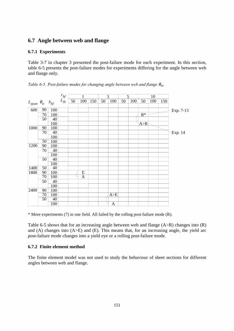
151
6.7 Angle between web and flange
6.7.1 Experiments
Table 3-7 in chapter 3 presented the post-failure mode for each experiment. In this section,table 6-5 presents the post-failure modes for experiments differing for the angle between weband flange only.
Table 6-5. Post-failure modes for changing angle between web and flange θw.
Lspan θw bbf
rbfLlb 50 100 150
150 100
350 100
550 100 150
10
70
50
50
7090
50
1200
14001800
24007090
50
100
10040
40100100
10040
10040
100100
AE
A>E
A
40
70 10090
50
600R*
100
A>R40
100
5090
1000
100100
9070
100
10040
Exp. 7-13
Exp. 14
* More experiments (7) in one field. All failed by the rolling post-failure mode (R).
Table 6-5 shows that for an increasing angle between web and flange (A>R) changes into (R)and (A) changes into (A>E) and (E). This means that, for an increasing angle, the yield arcpost-failure mode changes into a yield eye or a rolling post-failure mode.
6.7.2 Finite element method
The finite element model was not used to study the behaviour of sheet sections for differentangles between web and flange.
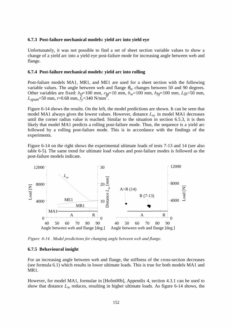
152
6.7.3 Post-failure mechanical models: yield arc into yield eye
Unfortunately, it was not possible to find a set of sheet section variable values to show achange of a yield arc into a yield eye post-failure mode for increasing angle between web andflange.
6.7.4 Post-failure mechanical models: yield arc into rolling
Post-failure models MA1, MR1, and ME1 are used for a sheet section with the followingvariable values. The angle between web and flange θw changes between 50 and 90 degrees.Other variables are fixed: btf=100 mm, rbf=10 mm, bw=100 mm, bbf=100 mm, Llb=50 mm,Lspan=50 mm, t=0.68 mm, fy=340 N/mm2.
Figure 6-14 shows the results. On the left, the model predictions are shown. It can be seen thatmodel MA1 always gives the lowest values. However, distance Lw in model MA1 decreasesuntil the corner radius value is reached. Similar to the situation in section 6.5.3, it is thenlikely that model MA1 predicts a rolling post-failure mode. Thus, the sequence is a yield arcfollowed by a rolling post-failure mode. This is in accordance with the findings of theexperiments.
Figure 6-14 on the right shows the experimental ultimate loads of tests 7-13 and 14 (see alsotable 6-5). The same trend for ultimate load values and post-failure modes is followed as thepost-failure models indicate.
40 50 60 70 80 90Angle between web and flange [deg.]
0
4000
8000
12000
0
10
20
30
Load
[N]
Dis
tanc
e L w
[mm
]
40 50 60 70 80 90Angle between web and flange [deg.]
4000
8000
12000
0
Load
[N]
A R A R
ME1MR1
MA1
Lw
A>R (14)R (7-13)
Figure 6-14. Model predictions for changing angle between web and flange.
6.7.5 Behavioural insight
For an increasing angle between web and flange, the stiffness of the cross-section decreases(see formula 6.1) which results in lower ultimate loads. This is true for both models MA1 andMR1.
However, for model MA1, formulae in [Hofm00b], Appendix 4, section 4.3.1 can be used toshow that distance Lw reduces, resulting in higher ultimate loads. As figure 6-14 shows, the
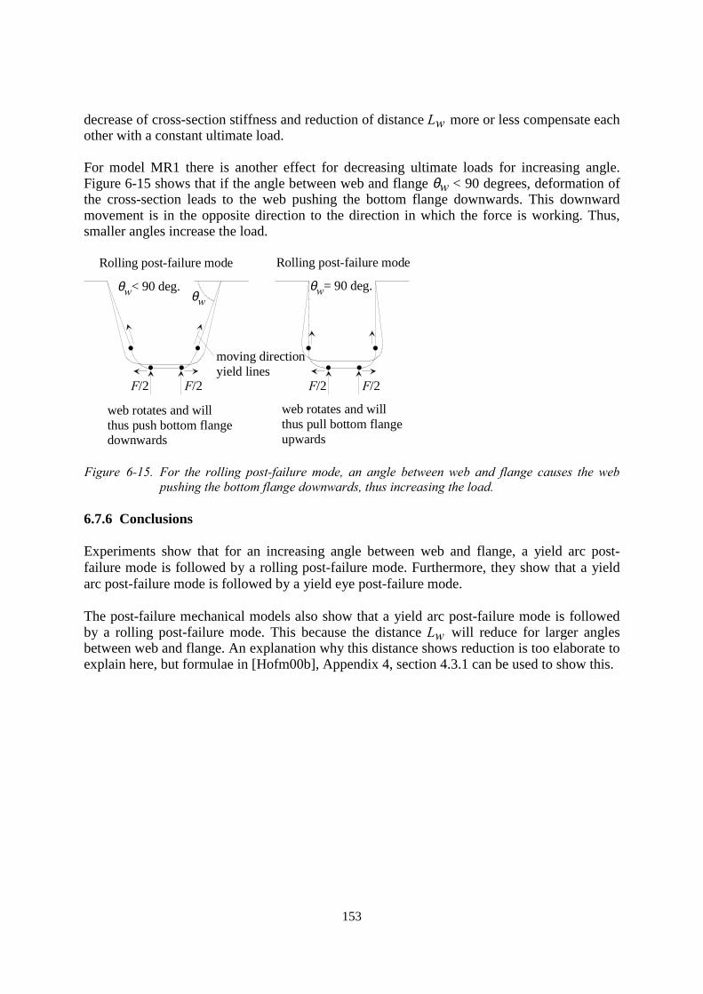
153
decrease of cross-section stiffness and reduction of distance Lw more or less compensate eachother with a constant ultimate load.
For model MR1 there is another effect for decreasing ultimate loads for increasing angle.Figure 6-15 shows that if the angle between web and flange θw < 90 degrees, deformation ofthe cross-section leads to the web pushing the bottom flange downwards. This downwardmovement is in the opposite direction to the direction in which the force is working. Thus,smaller angles increase the load.
Rolling post-failure mode
web rotates and willthus push bottom flangedownwards
web rotates and willthus pull bottom flangeupwards
F/2 F/2 F/2F/2
θwθw< 90 deg. θw= 90 deg.
moving directionyield lines
Rolling post-failure mode
Figure 6-15. For the rolling post-failure mode, an angle between web and flange causes the webpushing the bottom flange downwards, thus increasing the load.
6.7.6 Conclusions
Experiments show that for an increasing angle between web and flange, a yield arc post-failure mode is followed by a rolling post-failure mode. Furthermore, they show that a yieldarc post-failure mode is followed by a yield eye post-failure mode.
The post-failure mechanical models also show that a yield arc post-failure mode is followedby a rolling post-failure mode. This because the distance Lw will reduce for larger anglesbetween web and flange. An explanation why this distance shows reduction is too elaborate toexplain here, but formulae in [Hofm00b], Appendix 4, section 4.3.1 can be used to show this.
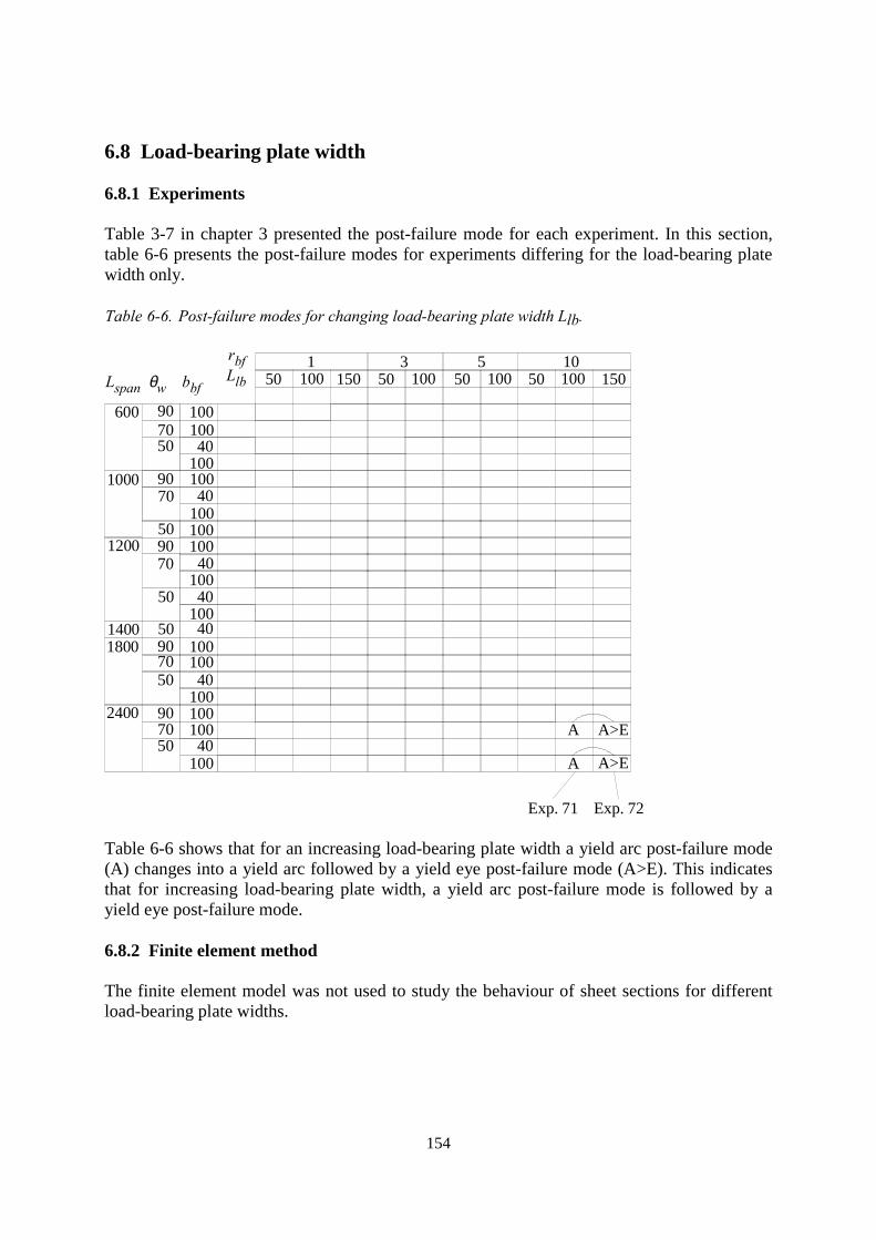
154
6.8 Load-bearing plate width
6.8.1 Experiments
Table 3-7 in chapter 3 presented the post-failure mode for each experiment. In this section,table 6-6 presents the post-failure modes for experiments differing for the load-bearing platewidth only.
Table 6-6. Post-failure modes for changing load-bearing plate width Llb.
Lspan θw bbf
rbfLlb 50 100 150
150 100
350 100
550 100 150
10
70
50
50
7090
50
1200
14001800
24007090
50
100
10040
40100100
10040
10040
100100 A>EA
A A>E
40
70 10090
50
600 100
40100
5090
1000
100100
9070
100
10040
Exp. 71 Exp. 72
Table 6-6 shows that for an increasing load-bearing plate width a yield arc post-failure mode(A) changes into a yield arc followed by a yield eye post-failure mode (A>E). This indicatesthat for increasing load-bearing plate width, a yield arc post-failure mode is followed by ayield eye post-failure mode.
6.8.2 Finite element method
The finite element model was not used to study the behaviour of sheet sections for differentload-bearing plate widths.
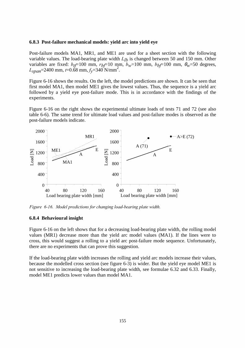
155
6.8.3 Post-failure mechanical models: yield arc into yield eye
Post-failure models MA1, MR1, and ME1 are used for a sheet section with the followingvariable values. The load-bearing plate width Llb is changed between 50 and 150 mm. Othervariables are fixed: btf=100 mm, rbf=10 mm, bw=100 mm, bbf=100 mm, θw=50 degrees,Lspan=2400 mm, t=0.68 mm, fy=340 N/mm2.
Figure 6-16 shows the results. On the left, the model predictions are shown. It can be seen thatfirst model MA1, then model ME1 gives the lowest values. Thus, the sequence is a yield arcfollowed by a yield eye post-failure mode. This is in accordance with the findings of theexperiments.
Figure 6-16 on the right shows the experimental ultimate loads of tests 71 and 72 (see alsotable 6-6). The same trend for ultimate load values and post-failure modes is observed as thepost-failure models indicate.
40 80 120 160Load bearing plate width [mm]
0
400
800
1200
1600
2000
Load
[N]
40 80 120 160Load bearing plate width [mm]
0
400
800
1200
1600
2000
Load
[N]
MA1
ME1
MR1
AE
AE
A (71)
A>E (72)
Figure 6-16. Model predictions for changing load-bearing plate width.
6.8.4 Behavioural insight
Figure 6-16 on the left shows that for a decreasing load-bearing plate width, the rolling modelvalues (MR1) decrease more than the yield arc model values (MA1). If the lines were tocross, this would suggest a rolling to a yield arc post-failure mode sequence. Unfortunately,there are no experiments that can prove this suggestion.
If the load-bearing plate width increases the rolling and yield arc models increase their values,because the modelled cross section (see figure 6-3) is wider. But the yield eye model ME1 isnot sensitive to increasing the load-bearing plate width, see formulae 6.32 and 6.33. Finally,model ME1 predicts lower values than model MA1.

156
6.8.5 Conclusions
Experiments suggest that for an increasing load-bearing plate width, a yield arc post-failuremode is followed by a yield eye post-failure mode. The post-failure mechanical models alsoshow that a yield arc post-failure mode is followed by a yield eye post-failure mode. This isbecause for the yield eye post-failure mode, only the bending moment in the section reducesdue to the larger load-bearing plate width. For the yield arc post-failure mode, the modelledcross-section is larger.
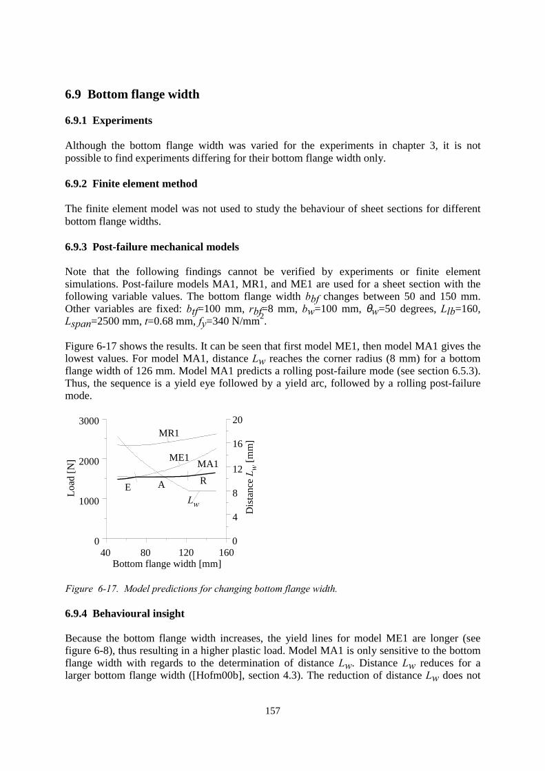
157
6.9 Bottom flange width
6.9.1 Experiments
Although the bottom flange width was varied for the experiments in chapter 3, it is notpossible to find experiments differing for their bottom flange width only.
6.9.2 Finite element method
The finite element model was not used to study the behaviour of sheet sections for differentbottom flange widths.
6.9.3 Post-failure mechanical models
Note that the following findings cannot be verified by experiments or finite elementsimulations. Post-failure models MA1, MR1, and ME1 are used for a sheet section with thefollowing variable values. The bottom flange width bbf changes between 50 and 150 mm.Other variables are fixed: btf=100 mm, rbf=8 mm, bw=100 mm, θw=50 degrees, Llb=160,Lspan=2500 mm, t=0.68 mm, fy=340 N/mm2.
Figure 6-17 shows the results. It can be seen that first model ME1, then model MA1 gives thelowest values. For model MA1, distance Lw reaches the corner radius (8 mm) for a bottomflange width of 126 mm. Model MA1 predicts a rolling post-failure mode (see section 6.5.3).Thus, the sequence is a yield eye followed by a yield arc, followed by a rolling post-failuremode.
40 80 120 160Bottom flange width [mm]
0
1000
2000
3000
0
4
8
12
16
20
Dis
tanc
e L w
[mm
]
Load
[N]
Lw
ME1
MR1
E A R
MA1
Figure 6-17. Model predictions for changing bottom flange width.
6.9.4 Behavioural insight
Because the bottom flange width increases, the yield lines for model ME1 are longer (seefigure 6-8), thus resulting in a higher plastic load. Model MA1 is only sensitive to the bottomflange width with regards to the determination of distance Lw. Distance Lw reduces for alarger bottom flange width ([Hofm00b], section 4.3). The reduction of distance Lw does not

158
have a large influence on the ultimate load. However, if distance Lw reaches the corner radiusvalue, a rolling post-failure mode is predicted.
6.9.5 Conclusions
Post-failure mechanical models show that for an increasing bottom flange width, a yield eyepost-failure mode is followed by a yield arc post-failure mode. Then, a yield arc post-failuremode is followed by a rolling post-failure mode.
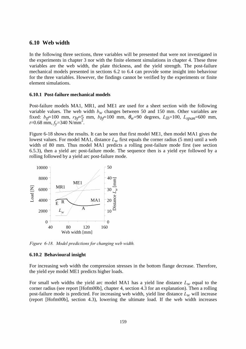
159
6.10 Web width
In the following three sections, three variables will be presented that were not investigated inthe experiments in chapter 3 nor with the finite element simulations in chapter 4. These threevariables are the web width, the plate thickness, and the yield strength. The post-failuremechanical models presented in sections 6.2 to 6.4 can provide some insight into behaviourfor the three variables. However, the findings cannot be verified by the experiments or finiteelement simulations.
6.10.1 Post-failure mechanical models
Post-failure models MA1, MR1, and ME1 are used for a sheet section with the followingvariable values. The web width bw changes between 50 and 150 mm. Other variables arefixed: btf=100 mm, rbf=5 mm, bbf=100 mm, θw=90 degrees, Llb=100, Lspan=600 mm,t=0.68 mm, fy=340 N/mm2.
Figure 6-18 shows the results. It can be seen that first model ME1, then model MA1 gives thelowest values. For model MA1, distance Lw first equals the corner radius (5 mm) until a webwidth of 80 mm. Thus model MA1 predicts a rolling post-failure mode first (see section6.5.3), then a yield arc post-failure mode. The sequence then is a yield eye followed by arolling followed by a yield arc post-failure mode.
MA1
40 80 120 160Web width [mm]
0
2000
4000
6000
8000
10000
0
10
20
30
40
50
Dis
tanc
e L w
[mm
]
Load
[N]
Lw
MR1ME1
EA
R
Figure 6-18. Model predictions for changing web width.
6.10.2 Behavioural insight
For increasing web width the compression stresses in the bottom flange decrease. Therefore,the yield eye model ME1 predicts higher loads.
For small web widths the yield arc model MA1 has a yield line distance Lw equal to thecorner radius (see report [Hofm00b], chapter 4, section 4.3 for an explanation). Then a rollingpost-failure mode is predicted. For increasing web width, yield line distance Lw will increase(report [Hofm00b], section 4.3), lowering the ultimate load. If the web width increases

160
further, rotation of the yield line in the web decreases for the same web crippling deformation(see section 6.2). Then the ultimate load slightly increases again.
6.10.3 Conclusions
Post-failure mechanical models show that for an increasing web width, a yield eye post-failure mode is followed by a rolling post-failure mode. Then, a rolling post-failure mode isfollowed by a yield arc post-failure mode.
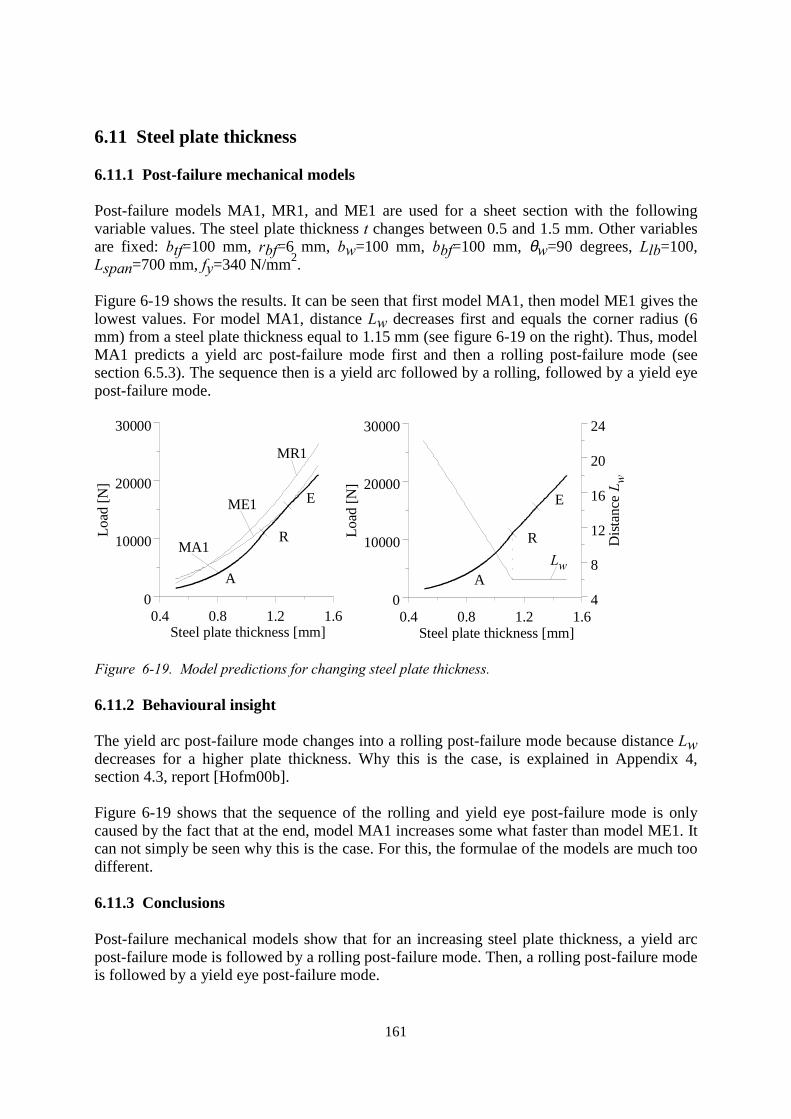
161
6.11 Steel plate thickness
6.11.1 Post-failure mechanical models
Post-failure models MA1, MR1, and ME1 are used for a sheet section with the followingvariable values. The steel plate thickness t changes between 0.5 and 1.5 mm. Other variablesare fixed: btf=100 mm, rbf=6 mm, bw=100 mm, bbf=100 mm, θw=90 degrees, Llb=100,Lspan=700 mm, fy=340 N/mm2.
Figure 6-19 shows the results. It can be seen that first model MA1, then model ME1 gives thelowest values. For model MA1, distance Lw decreases first and equals the corner radius (6mm) from a steel plate thickness equal to 1.15 mm (see figure 6-19 on the right). Thus, modelMA1 predicts a yield arc post-failure mode first and then a rolling post-failure mode (seesection 6.5.3). The sequence then is a yield arc followed by a rolling, followed by a yield eyepost-failure mode.
0.4 0.8 1.2 1.6Steel plate thickness [mm]
0
10000
20000
30000
Load
[N]
MA1
ME1
MR1
A
R
E
0.4 0.8 1.2 1.6Steel plate thickness [mm]
0
10000
20000
30000
4
8
12
16
20
24
Load
[N]
Dist
ance
Lw
LwA
R
E
Figure 6-19. Model predictions for changing steel plate thickness.
6.11.2 Behavioural insight
The yield arc post-failure mode changes into a rolling post-failure mode because distance Lwdecreases for a higher plate thickness. Why this is the case, is explained in Appendix 4,section 4.3, report [Hofm00b].
Figure 6-19 shows that the sequence of the rolling and yield eye post-failure mode is onlycaused by the fact that at the end, model MA1 increases some what faster than model ME1. Itcan not simply be seen why this is the case. For this, the formulae of the models are much toodifferent.
6.11.3 Conclusions
Post-failure mechanical models show that for an increasing steel plate thickness, a yield arcpost-failure mode is followed by a rolling post-failure mode. Then, a rolling post-failure modeis followed by a yield eye post-failure mode.
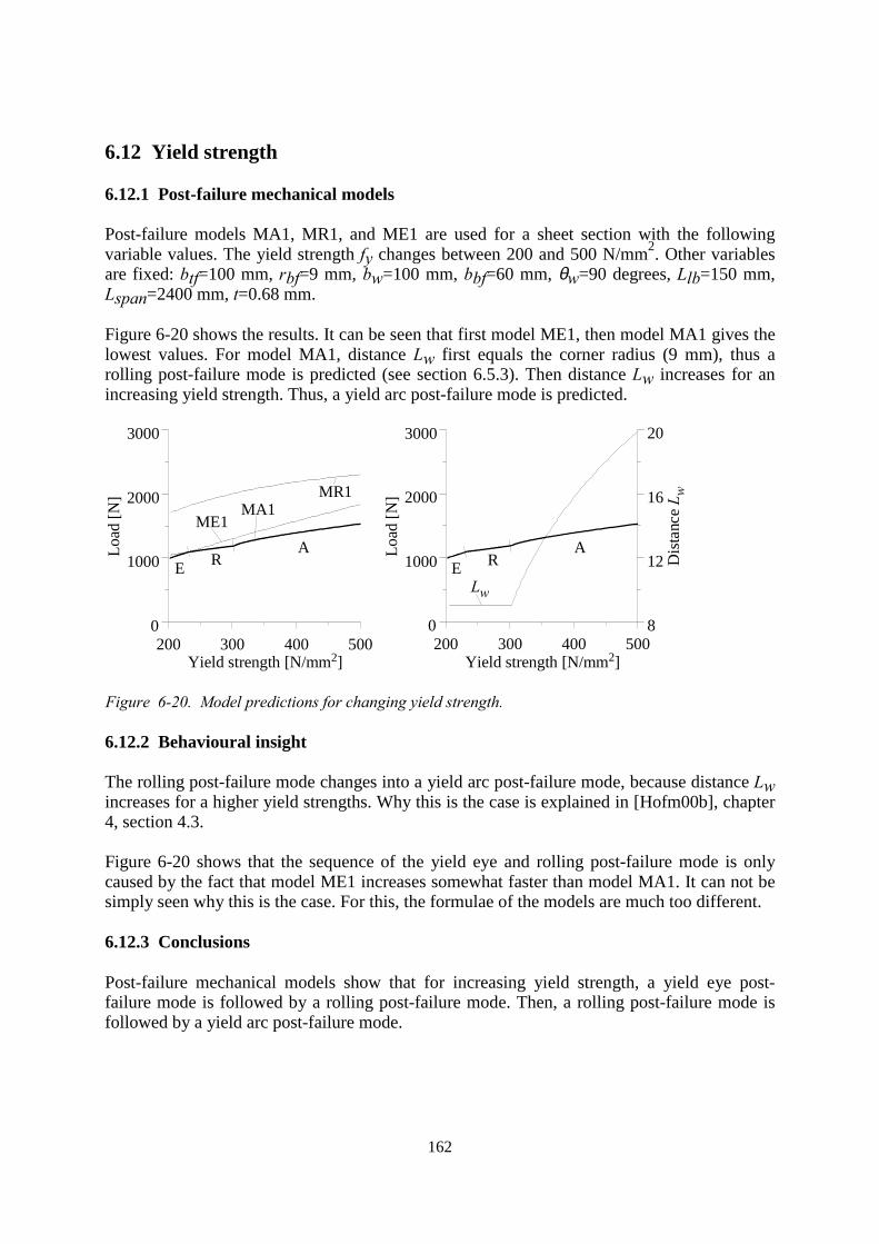
162
6.12 Yield strength
6.12.1 Post-failure mechanical models
Post-failure models MA1, MR1, and ME1 are used for a sheet section with the followingvariable values. The yield strength fy changes between 200 and 500 N/mm2. Other variablesare fixed: btf=100 mm, rbf=9 mm, bw=100 mm, bbf=60 mm, θw=90 degrees, Llb=150 mm,Lspan=2400 mm, t=0.68 mm.
Figure 6-20 shows the results. It can be seen that first model ME1, then model MA1 gives thelowest values. For model MA1, distance Lw first equals the corner radius (9 mm), thus arolling post-failure mode is predicted (see section 6.5.3). Then distance Lw increases for anincreasing yield strength. Thus, a yield arc post-failure mode is predicted.
200 300 400 500Yield strength [N/mm2]
0
1000
2000
3000
MR1
ME1MA1
EA
RLoad
[N]
200 300 400 500Yield strength [N/mm2]
0
1000
2000
3000
8
12
16
20
Lw
Dis
tanc
e L w
Load
[N]
EA
R
Figure 6-20. Model predictions for changing yield strength.
6.12.2 Behavioural insight
The rolling post-failure mode changes into a yield arc post-failure mode, because distance Lwincreases for a higher yield strengths. Why this is the case is explained in [Hofm00b], chapter4, section 4.3.
Figure 6-20 shows that the sequence of the yield eye and rolling post-failure mode is onlycaused by the fact that model ME1 increases somewhat faster than model MA1. It can not besimply seen why this is the case. For this, the formulae of the models are much too different.
6.12.3 Conclusions
Post-failure mechanical models show that for increasing yield strength, a yield eye post-failure mode is followed by a rolling post-failure mode. Then, a rolling post-failure mode isfollowed by a yield arc post-failure mode.

163
6.13 Conclusions
For two sheet section variables, namely the corner radius and span length, experiments, finiteelement simulations, and the post-failure mechanical models predict the same sequence ofpost-failure modes for the changing variable. The mechanical models provide insight intowhy a specific post-failure mode occurs.
For two variables, namely the angle between web and flange and the load-bearing plate width,experiments and post-failure mechanical models predict the same sequence of post-failuremodes for the changing variable. Again, the mechanical models provide insight into why aspecific post-failure mode occurs.
For the other variables, only post-failure models were used. The post-failure models explainwhy a certain post-failure modes occurs, but these findings cannot be verified becausesuitable experiments and finite element simulations are not available. Future research coulduse the finite element models (and more experiments) to extend the knowledge aboutbehaviour for changing variables.

164
7 Conclusions and recommendations
Chapter abstractSome important conclusions are given in this chapter. The conclusions of each individualchapter are not repeated. Recommendations are presented for future research.
165
7.1 Conclusions
7.1.1 Research aim
The aim of the research presented in this thesis was to provide better design rules for first-generation sheeting, specifically for the load case of combined bending and concentrated load,which are more accurate and provide more insight.
7.1.2 Results achieved
The experiments of chapter 3 show that after ultimate load, three post-failure modes arise: theyield arc, rolling, and yield eye post-failure modes. The finite element simulations show thatuntil and at ultimate load, there are two ultimate failure modes: the rolling and localised yieldultimate failure modes. Both the experiments and finite element simulations thus provideinsight into the physical behaviour of the sheeting.
Chapter 5 presents an ultimate failure mechanical model that performs equal to the currentdesign rules (Eurocode3). Because this is a mechanical model, it provides insight in thephysical behaviour of the sheeting.
Chapter 6 presents post-failure mechanical models that provide information on the sequenceof post-failure modes occurring for changing variables. Not all of these models perform wellcompared to the existing design rules (see [Hofm00b], chapter 2, section 2.5) and they are notmeant to be design rules. However, they provide additional insight into the sheetingbehaviour.
7.1.3 Scientific contribution
It is shown that current design rules still differ for some aspects and yield different results(chapter 2, section 2.1). However, as chapter 5 shows, Eurocode3 predictions are good for theexperiments investigated.
Experiments were carried out for which not only the ultimate load was recorded, but includethoroughly descriptions of the failure modes too.
Successful finite element models were developed. It was shown that an accurate modelling ofthe corners, the load application, and the appropriate use of a quarter or half model are allimportant for obtaining good results.
An ultimate failure mechanical model was developed. In this model elastic cross-sectiondeformations are used as imperfection in a non-linear observation of bottom flange behaviour.This is a completely new approach.
Post-failure mechanical models were developed. They provide new information on the reasonfor the occurrence of a certain post-failure mode.

166
7.1.4 Contribution to practice
A new and accurate model was developed (chapter 5) that can be used to predict the ultimateload of sheeting.
The post-failure mechanical models provide information on the reason for occurrence of aspecific post-failure mode. Therefore, these models can be used to improve sheeting design.
167
7.2 Future research, recommendations
7.2.1 Better cross-section models
In report [Hofm00b], chapter 4, section 4.3, a mechanical model was introduced to predict theplastic behaviour of sheet section cross-sections. With this model alone, it was possible topredict the whole plastic curve of the cross-section, for small and intermediate corner radii(The post-failure mechanical models introduced in chapter 6, section 6.2 and 6.3 were onlycapable of predicting the ultimate load of the cross-section. They were different for the rollingand yield arc post-failure modes). The mechanical model in report [Hofm00b], section 4.3could be used in the mechanical models of section 6.2 and 6.3. Advantages of the use of thismodel could be higher accuracy, description of plastic behaviour, and the need for only onemodel for two post-failure modes.
7.2.2 Simplification ultimate failure mechanical model
In the conclusions, it was stated that the ultimate failure mechanical model (chapter 5) couldbe used as a design rule. Although the model can be used on practically any personalcomputer with ease, it is not suitable for use by hand. The model could possibly be simplifiedin the same way as was already done for the post-failure mechanical models in report[Hofm00b], chapter 2 and 3.
7.2.3 Modern sheeting
At this time, the use of second and third-generation sheeting has almost completely replacedthe use of first-generation sheeting. Therefore, accurate and insightful design rules are neededfor these generations of sheeting. It is suggested that to develop these design rules, the samestrategy is used as presented in this thesis: Use experiments that simulate the situation inpractice. Develop finite element models that accurately simulate the experiments. Developmechanical models that can serve as a base for the new design rules.
7.2.4 Fitting of the mechanical models
In this thesis, fitting of mechanical models was not presented. To improve the quality of themodels, the models can be fitted to experiments. They can also be fitted to finite elementresults, thus avoiding the difference between imperfection sizes in practice and forexperiments in the laboratories. If this latter option is used, the models have to be fitted twice:first to the finite element results, then to imperfections occurring in practice.
168
Literature
[Acha98a] Acharya, V.V.; Schuster, R.M.: Bending Tests of Hat Sections with MultipleLongitudinal Stiffeners. Proceedings 14th International Specialty Conference on RecentResearch and Developments in Cold-Formed Steel Design and Construction, October 15-161998, St. Louis, Missouri, U.S.A.
[Aisi96a] Specification for the Design of Cold-Formed Steel Structural Members, 1996Edition, 1st. Printing-June 1997, American Iron and Steel Institute, 1101 17th Street, NW,Washington, DC 20036-4700, USA.
[Ande73a] Andersson, T.; Bergfors, A.: Upplagstryckets inverkan på brottlasten hostrapetsprofilerad plåt, Examenarbeite i Stålbyggnad, Stockholm, K.T.H., 1973.
[Ansy99a] Ansys 5.4, University High Option, ANSYS, Inc., Southpointe 275 TechnologyDrive, Canonsburg, PA 15317, 1999.
[Bahr78a] Bähr, Günter, Dr.-Ing.: Eine einfache Abschätzung der aufnehmbarenEndauflagerkräfte von Stahl-Trapezblechprofilen, Die Bautechnik, 11/1978, page 388-390.
[Bakk86a] Bakker, M.C.M.; Peköz, T.: Comparison and evaluation of web cripplingprediction formulas, Report of Eindhoven University of Technology, EUT 86-B-01, ISBN 90-6814-301-8, May 1986.
[Bakk92a] Bakker, Monique C.M.: Web Crippling of Cold-Formed Steel Members,Dissertation Eindhoven University of Technology, The Netherlands, ISBN 90-386-0122-0,1992.
[Bakk99a] Bakker, M.C.M., Snijder, H.H., Kerstens, J.G.M. Elastic Web Crippling of Thin-Walled Cold Formed Steel Members. Proceedings Light-Weight Steel and AluminiumStructures, Fourth International Conference on Steel and Aluminium Structures, Mäkeläinen,P; Hassinen, P., June 1999, Espoo, Finland.
[Berg73a] Bergfelt, Allan; Edlund, Bo; Larsson, Hans: Experiments on Trapezoidal SteelSheets in Bending, Third Speciality Conference on Cold-Formed Steel Structures, page 285-314, St. Louis, Missouri, USA, 1973.
[Berg79a] Bergfelt, A.; Edlund, B.: Effects of Web Buckling in Light Gauge Steel Beams,Thin-Walled Structures, TA 660 T5 I61, 1979, 427-440.
[Bern92a] Bernard, E.S.; Bridge, R.Q.; Hancock, G.J.: Tests of Profiled Steel Decks with V-Stiffeners, Proceedings 11th International Speciality Conference on Recent Research andDevelopments in Cold-Formed Steel Design and Construction, October 20-21 1992, St.Louis, Missouri, U.S.A.
[Bern93a] Bernard, Erik Stefan; Bridge, Russell Q.; Hancock, Gregory J.: Tests of ProfiledSteel Decks with V-stiffeners, Journal of Structural Engineering 119, 1993, page 2277-2293.
169
[Bern95a] Bernard, Erik Stefan; Bridge, Russell Q.; Hancock, Gregory J.: Tests on ProfiledSteel Decks with Flat-Hat Stiffeners, Journal of Structural Engineering 121, 1995, page 1175-1182.
[Bern96a] Bernard, E.S.; Bridge, R.Q.: Flange Curling in Profiled Steel Decks, Thin-WalledStructures 25, 1996, page 1-29.
[Bern96b] Bernard, Stefan E.; Bridge, Russell Q.; Hancock, Gregory J.: Design Methods forProfiled Steel Decks with Intermediate Stiffeners, Journal of Constructional Steel Research38, 1996, page 61-88.
[Bleu70a] Bleustein, Jeffrey L.; Gjelsvik, Atle: Rational Design of Light Gage Beams,Journal of the Structural Division, Proceedings of the American Society of Civil Engineers,Volume 96, Number ST7, July 1970.
[Cana95a] Canadian Standards Association: S136-94 (with General Instruction No. 2), ColdFormed Steel Structural Members, Structures (Design), Rexdale (Toronto), Ontario, Canada,May 1995.
[Coro96a] Corona, Edmundo; Vaze, Suhas P.: Buckling of Elastic-Plastic Square Tubes underBending, International Journal of Mechanical Sciences 38, 1996, page 753-775.
[Dann90a] Dannemann, Robert W.: Effective Width in Elastic Post-Buckling of Thin Flanges,Proceedings 10th International Speciality Conference on Recent Research and Developmentsin Cold-Formed Steel Design and Construction, October 23-24 1990, St. Louis, Missouri,U.S.A.
[Davi97a] Davies, J.M.; Jiang, C.: Design Procedures for Profiled Metal Sheeting andDecking, Thin-Walled Structures 27 (1997), 43-53.
[Davi99a] Davies, J.M.; Jiang, C.; Liu, Y.J.: Web Crippling in Trapezoidally ProfiledSheeting and Decking, Proceedings Eurosteel 1999, May 26-29, 1999, Praha, CzechRepublic.
[Dino63a] Deutsche norm DIN 50952, Prüfung metallischer Überzüge, Bestimmung desFlächengewichtes von Zinküberzügen auf Stahl durch chemisches Ablösen des Überzuges,Gravimetrisches Verfahren, Germany, December, 1963.
[Euro90a] European standard EN 10-002, Metallic materials - Tensile testing - Part 1: Methodof test (at ambient temperature), CEN European Committee for Standardisation, March 1990,correction AC1, June 1990.
[Euro96a] ENV 1993-1-3, European Prestandard Eurocode3, Design of Steel Structures, Part1-3: General rules-Supplementary rules for cold-formed thin gauge members and sheeting,European Committee for Standardisation CEN, Brussels, April 1996.
170
[Hair95a] Haironville Nederland B.V.: Profielschetsen van fabriek Haironville S.A., Frankrijk(June 16, 1995), Haironville Nederland B.V., P.O. Box 5660, 3008 AR, Rotterdam, TheNetherlands.
[Hofm96a] Hofmeyer, H.; Kerstens, J.G.M.; Snijder, H.H.; Bakker, M.C.M.: New ResearchDirections in Flexural Member Failure at an Interior Support (Interaction of Web Cripplingand Bending Moment), Proceedings European Workshop Thin-Walled Steel Structures,September 26-27 1996, Krzyzowa, Poland.
[Hofm96b] Hofmeyer, H.; Kerstens, J.G.M.; Snijder, H.H.; Bakker, M.C.M.: ExperimentalResearch on the Behaviour of Combined Web Crippling and Bending of Steel Deck Sections,Proceedings 13th International Speciality Conference on Recent Research and Developmentsin Cold-Formed Steel Design and Construction, October 17-18 1996, St. Louis, Missouri,U.S.A.
[Hofm99a] Hofmeyer, H.; Kerstens, J.G.M.; Snijder, H.H.; Bakker, M.C.M.: Numerical andAnalytical Modelling of Hat-Section Web Crippling Behaviour, Acta Polytechnica, Volume39, Number 5 / 1999, page 87-104.
[Hofm00b] Hofmeyer, H.: Report TUE-BCO-00-09: Report on Combined Web Crippling andBending Moment Failure of First-Generation Trapezoidal Steel Sheeting (Appendices to thethesis), Eindhoven University of Technology, Faculty of Architecture, Department ofStructural Design, The Netherlands, 2000, ISBN 90-6814-115-5.
[Hofm00c] Hofmeyer, H.; Kerstens, J.G.M.; Snijder, H.H.; Bakker, M.C.M.: FE Models forSheeting under Interaction Load, Proceedings 15th International Speciality Conference onRecent Research and Developments in Cold-Formed Steel Design and Construction, October19-20, 2000, St. Louis, Missouri, U.S.A.
[Kall77a] Källsner, Bo.: Post-Buckling Behaviour and Load-Carrying Capacity of Thin-Walled Box and Hat-Section Beams, Lund Institute of Technology, Division of BuildingTechnology, Report TVBK-1001, Lund, Sweden, 1977.
[Kárm31a] Kármán, Theodor von; Sechler, Ernest E.; Donnel, L.H.: The Strength of ThinPlates in Compression, Transactions of the American Society of Mechanical Engineers,APM-54-5, 1931.
[Keul80a] Keulers, A.J.C.: Report of the results concerning the effect of the load bearinglength on the failure load of a cold-formed steel sheet at an internal support, (Web-Crippling),Including a comparison of the test results with the provisional ECCS recommendations (80-02-15) concerning this subject, Report THE-BKO-S-80-2, Eindhoven University ofTechnology, Department of Structural Design, The Netherlands, 1980.
[Keul81a] Keulers, A.J.C.: Buigproeven en Interactieproeven. Een vergelijking vanproefresultaten met de ECCS-81 interactiecurve, waarbij deze curve gebaseerd is optestwaarden voor Md en Rd, i.p.v. op volgens de ECCS-81 berekende waarden. Report THE-
171
BKO-S-81-01, Eindhoven University of Technology, Department of Structural Design, TheNetherlands, 1981.
[Land94a] Landolfo, Raffaele; Mazzolani, Federico M.: Ultimate Behaviour of TrapezoidalSteel Sheets in Bending, Proceedings 12th International Speciality Conference on RecentResearch and Developments in Cold-Formed Steel Design and Construction, October 18-191994, St. Louis, Missouri, U.S.A.
[Land95a] Landolfo, Raffaele; Mazzolani, Frederico M.: Comportamento flessionale dilamiere grecate in acciaio: analisi sperimentale, Construczioni Metalliche 29, N. 1 Gennaio-Febbraio 1995.
[Lind96a] Lindner, Univ.-Prof. Dr.-Ing. Joachim; Shin, Dr.-Ing. Tae Song: Interactionbetween Flexural Buckling and Plate Buckling on the Web Crippling Capacity of TrapezoidalSheeting, Conference Proceedings of the Second International Conference on CoupledInstabilities in Metal Structures CIMS, September 5-7, 1996, Liege, Belgium.
[Luur93a] Luure, Pritt; Crisinel, Michel: Redistribution of Moments at the Interior Supportfor Cold Formed Sheeting, ICOM 288, EPFL-École polytechnique fédérale de Lausanne,ICOM-Construction métallique, CH-1015 Lausanne, 1993.
[Marg38a] Marguerre, K.: Zur Theorie der gekrümmter Platte grosser Formänderung, Proc.Fifth. Int. Congress Appl. Mech., Page 93, 1938.
[Murr81a] Murray, N.W.; Khoo, P.S.: Some Basic Plastic Mechanisms in the Local Bucklingof Thin-Walled Steel Structures, International Journal of Mechanical Science, Vol. 23, No.12, page 703-713, 1981.
[Murr85a] Murray, Noel W.: Introduction to the Theory of Thin-Walled Structures, OxfordEngineering Science Series 13, Clarendon Press Oxford, ISBN 0-19-856186-5, 1985.
[Nest81a] Van Neste, prof. ir. A.J.: Berekening van stalen dakplaten, Bouwen met Staal 56,1981, page 26-31.
[Orto88a] Orton, Andrew: The way we build now: form, scale and technique, Published byVan Nostrand Reinhold (UK) Co. Ltd., Molly Millars Lane, Wokingham, Berkshire, England,ISBN 0-74760011-2, 1988.
[Park96a] Park, M.S.; Lee, B.C.: Prediction of Mode Parameters and Moment-RotationCurves for Crushed Thin-Walled Trapezoidal Tubes in Bending, Journal of AppliedMechanics 63, 1996, page 453-459.
[Reck75a] Reck, Peter H.; Peköz, Teoman; Winter, George: Inelastic Strength of Cold-Formed Steel Beams, Journal of the Structural Devision, Vol. 101, No. ST11, November1975, page 2193-2203.
[Rein83a] Reinsch, W.: Das Kantenbeulen zur rechnerischen Ermittlung vonStahltrapezblechträger, dissertation D17, Technische Hochschule Darmstadt, Germany, 1983.
172
[Rhod99a] Rhodes, J.; Nash, D.; Macdonald, M.: An Examination of Web Crushing in Thin-Walled Beams, Proceedings Light-Weight Steel and Aluminium Structures, FourthInternational Conference on Steel and Aluminium Structures, Mäkeläinen, P; Hassinen, P.,20-23 June 1999, Espoo, Finland, page 795-802.
[Rsdm74a] Richtlijnen voor de berekening van Stalen Dakplaten-RSD 1974, Dumebo enStaalbouwkundig Genootschap, The Netherlands, 1974.
[Sabp95a] SAB-Profiel B.V.: Leveringsprogramma (June 16, 1995), SAB-Profiel B.V.,P.O.Box 97, 3400 AB, IJsselstein, The Netherlands.
[Sama99a] Samanta, Asokendu; Mukhopadhyay, Madhujit: Finite element static and dynamicanalyses of folded plates, Engineering Structures 21, 1999, page 277-287.
[Sant86a] Santaputra, C.: Eighth progress report, Design of Automotive StructuralComponents using High Strength Sheet Steels, Web Crippling of Cold Formed Steel Beams,Civil Engineering Study 86-1, Structural Series, University of Missouri-Rolla, Department ofCivil Engineering, 1986.
[Scha97a] Schafer, B.W.; Peköz, T.: The Behaviour and Design of Longitudinally StiffenedThin-Walled Compression Elements, Thin-Walled Structures Vol. 27, 1997, page 65-78.
[Scha98a] Schafer, B.W.; Peköz, T.: Direct Strength Prediction of Cold-Formed SteelMembers Using Numerical Elastic Buckling Solutions, Proceedings 14th InternationalSpecialty Conference on Recent Research and Developments in Cold-Formed Steel Designand Construction, October 15-16 1998, St. Louis, Missouri, USA.
[Sche90a] Scherpbier, Gerbrand: Globaal konstruktief ontwerpen, Lecture notes, EindhovenUniversity of Technology, Department of Structural Design, Eindhoven,The Netherlands, 1990.
[Shan84a] Shanmugam, Nandivaram E.; Lee, Seng-Lip: Ultimate Load Behaviour ofTrapezoidal Steel Decks, Journal of Structural Engineering 110, 1984, page 1747-1756.
[Shar89a] Sharp, M.L.: Behaviour of plates under partial edge loading, Steel StructuresProceedings, Structures Congress 1989, San Francisco, ASCE, 1989.
[Shar90a] Sharp, M.L.: Design parameters for web crippling of thin-walled members, reportNo. 57-90-21, Alcoa laboratories, 1990.
[Soko97a] Sokol, Leopold: Some Specific Aspects of Elastic-Plastic Behaviour of ProfiledSteel Sheeting and Decking, Thin-Walled Structures 29, 1997, page 101-112.
[Soko98a] Sokol, Leopold: A Non Linear Design Model for Continuous Multi-Span LightGauge Sheeting and Members, Proceedings 14th International Specialty Conference onRecent Research and Developments in Cold-Formed Steel Design and Construction, October15-16 1998, St. Louis, Missouri, U.S.A.
173
[Stud90a] Studnicka, J.: Web crippling of wide deck sections, Recent Research andDevelopments in Cold-Formed Steel Design and Construction, Edited by W.W. Yu and R.A.Laboube, Rolla, University of Missouri-Rolla, Department of Civil Engineering, 1990.
[Talj92a] Talja, Asko: Design of cold-formed HSS channels for bending and eccentriccompression., Bending in the plane of symmetry, VTT Research Notes 1403, TechnicalResearch Centre of Finland, Espoo, 1992.
[Thom96a] Thomopoulos, K.T.; Mistakidis, E.S.; Koltsakis, E.K.; Panagiotopoulos, P.D.:Softening Behaviour of Continuous Thin-walled Steel Beams, Two Numerical Methods,Journal of Constructional Steel Research 36, 1996, page 1-13.
[Toma73a] Tomà, A.; Stark, J.W.B.: II. Vrij opgelegde platen op twee steunpunten zonderdimpels, Onderzoek geprofileerde stalen dakplaten, werkrapport van de werkgroep S.G.-T.C.16 "Onderzoek van stalen dak- en gevelplaten", Instituut TNO voor bouwmaterialen enbouwconstructies, rapport nr. BI-73-75, Opdr. nr. 05.3.11.260, September 1973.
[Toma74a] Tomà, A.; Stark, J.W.B.: III. Twee veldsplaten zonder dimpel, Onderzoekgeprofileerde stalen dakplaten, werkrapport van de werkgroep S.G.-T.C. 16 "Onderzoek vanstalen dak- en gevelplaten", Instituut TNO voor bouwmaterialen en bouwconstructies, rapportnr. BI-74-37, Nr. 05.3.11.261, April 1974.
[Tsai86a] Tsai, Y.M.; Crisinel, M.: Moment redistribution in continuous profiled sheeting,Thin-walled metal structures in buildings, IABSE proceedings, Vol. 49, page 107-114,Zürich: IABSE-AIPC-IVBH, 1996.
[Unge73a] Unger, B.: Ein Beitrag zur Ermittlung der Traglast von querbelastetenDurchlaufträgern mit dünnwandigem Querschnitt, insbesondere von durchlaufendenTrapezblechen für Dach und Geschoß decken, Der Stahlbau 1-1973, page 20-24.
[Vaes95a] Vaessen, M.J.: On the elastic web crippling stiffness of thin-walled cold-formedsteel members, MSc. thesis, Eindhoven University of Technology, Department of StructuralDesign, The Netherlands, 1995.
[Wang73a] Wang, Shien T.: Non-linear Analysis of Thin-Walled Continuous Beams,Proceedings 2nd International Speciality Conference on Recent Research and Developmentsin Cold-Formed Steel Design and Construction, October 22-24 1973, St. Louis, Missouri,U.S.A.
[Wing81a] Wing, B.A.: Web crippling and the interaction of bending and web crippling ofunreinforced multi-web cold-formed steel sections, Master's thesis, Waterloo, University ofWaterloo, 1981.
[Wint49a] Winter, G.: Strength of Thin Steel Compression Flanges, with appendix, bulletin35/3, Cornell University Engineering Experiment Station, Ithaca, NY, 1947.

174
[Wise91a] Wiseman, D.L.; Puckett, J.A1.: Applications of Compound Strip Method forFolded Plates with Connection Elements, Journal of Structural Engineering 117, 1991, 268-285.
[Wuyu98a] Wu, Shaojie; Yu, Wei-Wen; LaBoube, Roger A.: Web Crippling Strength ofMembers using High-Strength Steels, Proceedings 14th International Specialty Conference onRecent Research and Developments in Cold-Formed Steel Design and Construction, October15-16 1998, St. Louis, Missouri, U.S.A.
[Yene85a] Yener, Muzaffer; Peköz, Teoman: Partial Moment Redistribution in Cold-FormedSteel, Journal of Structural Engineering, Vol. 111, No. 6, June, 1985.
[Yuww85a] Yu, Wei-Wen: Cold-Formed Steel Design, A Wiley-Interscience publication,ISBN 0-471-88484-7, 1985.
[Zetl52a] Zetlin, L.; Winter, G.: 65th. and 66th. progress reports on light gauge steel beams ofcold-formed steel, unpublished, Ithaca, Cornell University, 1952.
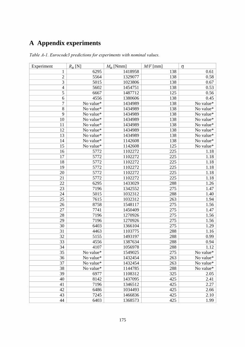
175
A Appendix experiments
Table A-1. Eurocode3 predictions for experiments with nominal values.
Experiment Ru [N] Mu [Nmm] M/F [mm] η1 6295 1418958 138 0.612 5564 1329077 138 0.583 5015 1023806 138 0.674 5602 1454751 138 0.535 6667 1487712 125 0.566 4556 1380606 138 0.457 No value* 1434989 138 No value*8 No value* 1434989 138 No value*9 No value* 1434989 138 No value*
10 No value* 1434989 138 No value*11 No value* 1434989 138 No value*12 No value* 1434989 138 No value*13 No value* 1434989 138 No value*14 No value* 1142608 138 No value*15 No value* 1142608 125 No value*16 5772 1102272 225 1.1817 5772 1102272 225 1.1818 5772 1102272 225 1.1819 5772 1102272 225 1.1820 5772 1102272 225 1.1821 5772 1102272 225 1.1822 6295 1433029 288 1.2623 7196 1342552 275 1.4724 5015 1032312 288 1.4025 7615 1032312 263 1.9426 8758 1548117 275 1.5627 7741 1450409 275 1.4728 7196 1270926 275 1.5629 7196 1270926 275 1.5630 6403 1366104 275 1.2931 4463 1103775 288 1.1632 5155 1493197 288 0.9933 4556 1387634 288 0.9434 4107 1056978 288 1.1235 No value* 1549025 275 No value*36 No value* 1432454 263 No value*37 No value* 1432454 263 No value*38 No value* 1144785 288 No value*39 6977 1108312 325 2.0540 8142 1437095 425 2.4141 7196 1346512 425 2.2742 6486 1034493 425 2.6643 7245 1466836 425 2.1044 6403 1368573 425 1.99
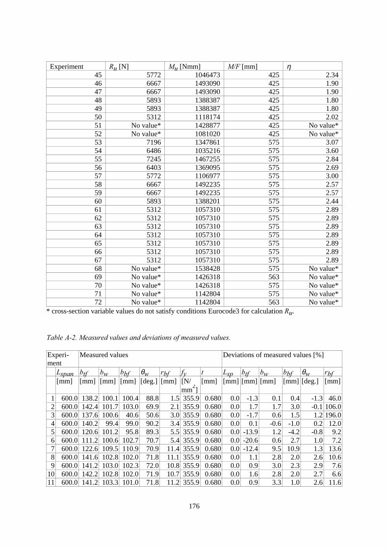
176
Experiment Ru [N] Mu [Nmm] M/F [mm] η45 5772 1046473 425 2.3446 6667 1493090 425 1.9047 6667 1493090 425 1.9048 5893 1388387 425 1.8049 5893 1388387 425 1.8050 5312 1118174 425 2.0251 No value* 1428877 425 No value*52 No value* 1081020 425 No value*53 7196 1347861 575 3.0754 6486 1035216 575 3.6055 7245 1467255 575 2.8456 6403 1369095 575 2.6957 5772 1106977 575 3.0058 6667 1492235 575 2.5759 6667 1492235 575 2.5760 5893 1388201 575 2.4461 5312 1057310 575 2.8962 5312 1057310 575 2.8963 5312 1057310 575 2.8964 5312 1057310 575 2.8965 5312 1057310 575 2.8966 5312 1057310 575 2.8967 5312 1057310 575 2.8968 No value* 1538428 575 No value*69 No value* 1426318 563 No value*70 No value* 1426318 575 No value*71 No value* 1142804 575 No value*72 No value* 1142804 563 No value*
* cross-section variable values do not satisfy conditions Eurocode3 for calculation Ru.
Table A-2. Measured values and deviations of measured values.
Experi-ment
Measured values Deviations of measured values [%]
Lspan btf bw bbf θw rbf fy t Lsp btf bw bbf θw rbf[mm] [mm] [mm] [mm] [deg.] [mm] [N/
mm2][mm] [mm] [mm] [mm] [mm] [deg.] [mm]
1 600.0 138.2 100.1 100.4 88.8 1.5 355.9 0.680 0.0 -1.3 0.1 0.4 -1.3 46.02 600.0 142.4 101.7 103.0 69.9 2.1 355.9 0.680 0.0 1.7 1.7 3.0 -0.1 106.03 600.0 137.6 100.6 40.6 50.6 3.0 355.9 0.680 0.0 -1.7 0.6 1.5 1.2 196.04 600.0 140.2 99.4 99.0 90.2 3.4 355.9 0.680 0.0 0.1 -0.6 -1.0 0.2 12.05 600.0 120.6 101.2 95.8 89.3 5.5 355.9 0.680 0.0 -13.9 1.2 -4.2 -0.8 9.26 600.0 111.2 100.6 102.7 70.7 5.4 355.9 0.680 0.0 -20.6 0.6 2.7 1.0 7.27 600.0 122.6 109.5 110.9 70.9 11.4 355.9 0.680 0.0 -12.4 9.5 10.9 1.3 13.68 600.0 141.6 102.8 102.0 71.8 11.1 355.9 0.680 0.0 1.1 2.8 2.0 2.6 10.69 600.0 141.2 103.0 102.3 72.0 10.8 355.9 0.680 0.0 0.9 3.0 2.3 2.9 7.6
10 600.0 142.2 102.8 102.0 71.9 10.7 355.9 0.680 0.0 1.6 2.8 2.0 2.7 6.611 600.0 141.2 103.3 101.0 71.8 11.2 355.9 0.680 0.0 0.9 3.3 1.0 2.6 11.6
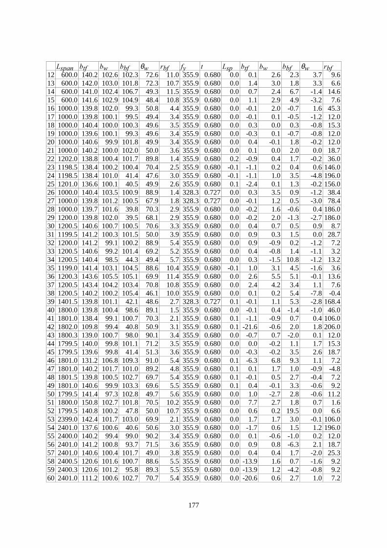
177
Lspan btf bw bbf θw rbf fy t Lsp btf bw bbf θw rbf12 600.0 140.2 102.6 102.3 72.6 11.0 355.9 0.680 0.0 0.1 2.6 2.3 3.7 9.613 600.0 142.0 103.0 101.8 72.3 10.7 355.9 0.680 0.0 1.4 3.0 1.8 3.3 6.614 600.0 141.0 102.4 106.7 49.3 11.5 355.9 0.680 0.0 0.7 2.4 6.7 -1.4 14.615 600.0 141.6 102.9 104.9 48.4 10.8 355.9 0.680 0.0 1.1 2.9 4.9 -3.2 7.616 1000.0 139.8 102.0 99.3 50.8 4.4 355.9 0.680 0.0 -0.1 2.0 -0.7 1.6 45.317 1000.0 139.8 100.1 99.5 49.4 3.4 355.9 0.680 0.0 -0.1 0.1 -0.5 -1.2 12.018 1000.0 140.4 100.0 100.3 49.6 3.5 355.9 0.680 0.0 0.3 0.0 0.3 -0.8 15.319 1000.0 139.6 100.1 99.3 49.6 3.4 355.9 0.680 0.0 -0.3 0.1 -0.7 -0.8 12.020 1000.0 140.6 99.9 101.8 49.9 3.4 355.9 0.680 0.0 0.4 -0.1 1.8 -0.2 12.021 1000.0 140.2 100.0 102.0 50.0 3.6 355.9 0.680 0.0 0.1 0.0 2.0 0.0 18.722 1202.0 138.8 100.4 101.7 89.8 1.4 355.9 0.680 0.2 -0.9 0.4 1.7 -0.2 36.023 1198.5 138.4 100.2 100.4 70.4 2.5 355.9 0.680 -0.1 -1.1 0.2 0.4 0.6 146.024 1198.5 138.4 101.0 41.4 47.6 3.0 355.9 0.680 -0.1 -1.1 1.0 3.5 -4.8 196.025 1201.0 136.6 100.1 40.5 49.9 2.6 355.9 0.680 0.1 -2.4 0.1 1.3 -0.2 156.026 1000.0 140.4 103.5 100.9 88.9 1.4 328.3 0.727 0.0 0.3 3.5 0.9 -1.2 38.427 1000.0 139.8 101.2 100.5 67.9 1.8 328.3 0.727 0.0 -0.1 1.2 0.5 -3.0 78.428 1000.0 139.7 101.6 39.8 70.3 2.9 355.9 0.680 0.0 -0.2 1.6 -0.6 0.4 186.029 1200.0 139.8 102.0 39.5 68.1 2.9 355.9 0.680 0.0 -0.2 2.0 -1.3 -2.7 186.030 1200.5 140.6 100.7 100.5 70.6 3.3 355.9 0.680 0.0 0.4 0.7 0.5 0.9 8.731 1199.5 141.2 100.3 101.5 50.0 3.9 355.9 0.680 0.0 0.9 0.3 1.5 0.0 28.732 1200.0 141.2 99.1 100.2 88.9 5.4 355.9 0.680 0.0 0.9 -0.9 0.2 -1.2 7.233 1200.5 140.6 99.2 101.4 69.2 5.2 355.9 0.680 0.0 0.4 -0.8 1.4 -1.1 3.234 1200.5 140.4 98.5 44.3 49.4 5.7 355.9 0.680 0.0 0.3 -1.5 10.8 -1.2 13.235 1199.0 141.4 103.1 104.5 88.6 10.4 355.9 0.680 -0.1 1.0 3.1 4.5 -1.6 3.636 1200.3 143.6 105.5 105.1 69.9 11.4 355.9 0.680 0.0 2.6 5.5 5.1 -0.1 13.637 1200.5 143.4 104.2 103.4 70.8 10.8 355.9 0.680 0.0 2.4 4.2 3.4 1.1 7.638 1200.5 140.2 100.2 105.4 46.1 10.0 355.9 0.680 0.0 0.1 0.2 5.4 -7.8 -0.439 1401.5 139.8 101.1 42.1 48.6 2.7 328.3 0.727 0.1 -0.1 1.1 5.3 -2.8 168.440 1800.0 139.8 100.4 98.6 89.1 1.5 355.9 0.680 0.0 -0.1 0.4 -1.4 -1.0 46.041 1801.0 138.4 99.1 100.7 70.3 2.1 355.9 0.680 0.1 -1.1 -0.9 0.7 0.4 106.042 1802.0 109.8 99.4 40.8 50.9 3.1 355.9 0.680 0.1 -21.6 -0.6 2.0 1.8 206.043 1800.3 139.0 100.7 98.0 90.1 3.4 355.9 0.680 0.0 -0.7 0.7 -2.0 0.1 12.044 1799.5 140.0 99.8 101.1 71.2 3.5 355.9 0.680 0.0 0.0 -0.2 1.1 1.7 15.345 1799.5 139.6 99.8 41.4 51.3 3.6 355.9 0.680 0.0 -0.3 -0.2 3.5 2.6 18.746 1801.0 131.2 106.8 109.3 91.0 5.4 355.9 0.680 0.1 -6.3 6.8 9.3 1.1 7.247 1801.0 140.2 101.7 101.0 89.2 4.8 355.9 0.680 0.1 0.1 1.7 1.0 -0.9 -4.848 1801.5 139.8 100.5 102.7 69.7 5.4 355.9 0.680 0.1 -0.1 0.5 2.7 -0.4 7.249 1801.0 140.6 99.9 103.3 69.6 5.5 355.9 0.680 0.1 0.4 -0.1 3.3 -0.6 9.250 1799.5 141.4 97.3 102.8 49.7 5.6 355.9 0.680 0.0 1.0 -2.7 2.8 -0.6 11.251 1800.0 150.8 102.7 101.8 70.5 10.2 355.9 0.680 0.0 7.7 2.7 1.8 0.7 1.652 1799.5 140.8 100.2 47.8 50.0 10.7 355.9 0.680 0.0 0.6 0.2 19.5 0.0 6.653 2399.0 142.4 101.7 103.0 69.9 2.1 355.9 0.680 0.0 1.7 1.7 3.0 -0.1 106.054 2401.0 137.6 100.6 40.6 50.6 3.0 355.9 0.680 0.0 -1.7 0.6 1.5 1.2 196.055 2400.0 140.2 99.4 99.0 90.2 3.4 355.9 0.680 0.0 0.1 -0.6 -1.0 0.2 12.056 2401.0 141.2 100.8 93.7 71.5 3.6 355.9 0.680 0.0 0.9 0.8 -6.3 2.1 18.757 2401.0 140.6 100.4 101.7 49.0 3.8 355.9 0.680 0.0 0.4 0.4 1.7 -2.0 25.358 2400.5 120.6 101.6 100.7 88.6 5.5 355.9 0.680 0.0 -13.9 1.6 0.7 -1.6 9.259 2400.3 120.6 101.2 95.8 89.3 5.5 355.9 0.680 0.0 -13.9 1.2 -4.2 -0.8 9.260 2401.0 111.2 100.6 102.7 70.7 5.4 355.9 0.680 0.0 -20.6 0.6 2.7 1.0 7.2
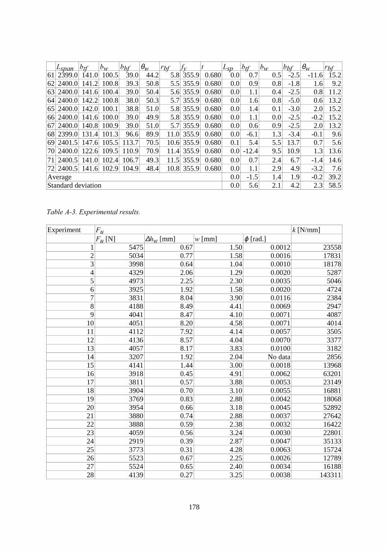
178
Lspan btf bw bbf θw rbf fy t Lsp btf bw bbf θw rbf61 2399.0 141.0 100.5 39.0 44.2 5.8 355.9 0.680 0.0 0.7 0.5 -2.5 -11.6 15.262 2400.0 141.2 100.8 39.3 50.8 5.5 355.9 0.680 0.0 0.9 0.8 -1.8 1.6 9.263 2400.0 141.6 100.4 39.0 50.4 5.6 355.9 0.680 0.0 1.1 0.4 -2.5 0.8 11.264 2400.0 142.2 100.8 38.0 50.3 5.7 355.9 0.680 0.0 1.6 0.8 -5.0 0.6 13.265 2400.0 142.0 100.1 38.8 51.0 5.8 355.9 0.680 0.0 1.4 0.1 -3.0 2.0 15.266 2400.0 141.6 100.0 39.0 49.9 5.8 355.9 0.680 0.0 1.1 0.0 -2.5 -0.2 15.267 2400.0 140.8 100.9 39.0 51.0 5.7 355.9 0.680 0.0 0.6 0.9 -2.5 2.0 13.268 2399.0 131.4 101.3 96.6 89.9 11.0 355.9 0.680 0.0 -6.1 1.3 -3.4 -0.1 9.669 2401.5 147.6 105.5 113.7 70.5 10.6 355.9 0.680 0.1 5.4 5.5 13.7 0.7 5.670 2400.0 122.6 109.5 110.9 70.9 11.4 355.9 0.680 0.0 -12.4 9.5 10.9 1.3 13.671 2400.5 141.0 102.4 106.7 49.3 11.5 355.9 0.680 0.0 0.7 2.4 6.7 -1.4 14.672 2400.5 141.6 102.9 104.9 48.4 10.8 355.9 0.680 0.0 1.1 2.9 4.9 -3.2 7.6Average 0.0 -1.5 1.4 1.9 -0.2 39.2Standard deviation 0.0 5.6 2.1 4.2 2.3 58.5
Table A-3. Experimental results.
Experiment Fu k [N/mm]Fu [N] ∆hw [mm] w [mm] ϕ [rad.]
1 5475 0.67 1.50 0.0012 235582 5034 0.77 1.58 0.0016 178313 3998 0.64 1.04 0.0010 181784 4329 2.06 1.29 0.0020 52875 4973 2.25 2.30 0.0035 50466 3925 1.92 1.58 0.0020 47247 3831 8.04 3.90 0.0116 23848 4188 8.49 4.41 0.0069 29479 4041 8.47 4.10 0.0071 4087
10 4051 8.20 4.58 0.0071 401411 4112 7.92 4.14 0.0057 350512 4136 8.57 4.04 0.0070 337713 4057 8.17 3.83 0.0100 318214 3207 1.92 2.04 No data 285615 4141 1.44 3.00 0.0018 1396816 3918 0.45 4.91 0.0062 6320117 3811 0.57 3.88 0.0053 2314918 3904 0.70 3.10 0.0055 1688119 3769 0.83 2.88 0.0042 1806820 3954 0.66 3.18 0.0045 5289221 3880 0.74 2.88 0.0037 2764222 3888 0.59 2.38 0.0032 1642223 4059 0.56 3.24 0.0030 2280124 2919 0.39 2.87 0.0047 3513325 3773 0.31 4.28 0.0063 1572426 5523 0.67 2.25 0.0026 1278927 5524 0.65 2.40 0.0034 1618828 4139 0.27 3.25 0.0038 143311
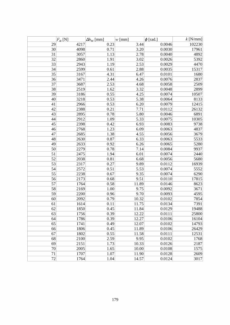
179
Fu [N] ∆hw [mm] w [mm] ϕ [rad.] k [N/mm]29 4217 0.23 3.44 0.0046 10223030 4098 0.71 3.20 0.0030 1796131 3057 1.13 2.78 0.0040 489232 2860 1.91 3.02 0.0026 539233 2943 1.19 2.53 0.0029 447034 2599 0.61 2.88 0.0035 1531735 3167 4.31 6.47 0.0101 168036 3471 2.44 4.26 0.0076 283737 3687 2.53 4.68 0.0058 250938 2519 1.62 3.32 0.0048 289939 3186 0.55 4.25 0.0074 1050740 3218 0.53 5.38 0.0064 813341 2966 0.53 6.20 0.0079 1241542 2388 0.21 7.71 0.0112 2613243 2895 0.78 5.80 0.0046 689144 2912 1.09 5.33 0.0075 1030545 2398 0.42 6.93 0.0083 973846 2768 1.23 6.09 0.0063 483747 2685 1.38 4.55 0.0056 367948 2630 0.87 6.33 0.0063 553349 2633 0.92 6.26 0.0065 528050 2279 0.78 7.14 0.0084 993751 2475 1.94 6.01 0.0074 244052 2038 0.81 6.68 0.0056 568053 2317 0.27 9.89 0.0112 1693954 2572 0.51 5.53 0.0074 555255 2238 0.67 9.35 0.0074 629056 2173 0.68 9.51 0.0110 1781557 1764 0.58 11.89 0.0146 862358 2169 1.00 9.75 0.0092 367159 2200 0.96 9.70 0.0093 459560 2092 0.79 10.32 0.0102 785461 1614 0.11 11.75 0.0134 739162 1850 0.45 11.84 0.0129 1948863 1756 0.39 12.22 0.0111 2580064 1786 0.39 12.27 0.0106 1610465 1741 0.49 12.07 0.0102 1479366 1806 0.45 11.89 0.0106 2642967 1802 0.55 11.58 0.0111 1253168 2100 2.59 9.95 0.0102 176869 2151 1.73 10.33 0.0126 218770 2005 1.65 10.00 0.0108 157571 1707 1.07 11.90 0.0128 260972 1764 1.04 14.57 0.0124 3017

180
Table A-4. Post-failure modes and yield line distances (all in [mm]).
Experi-ment
Post-failuremode
Lw Lbf;left;out
Lbf;left;in
Lbf;left;edge
Lbf;right;out
Lbf;right;in
Lbf;right;edge
Ltf L-2Ltf
1 A>R * 32 0 25 35 0 25 502 A>R 47 0 35 47 0 35 493 A>R 28 0 21 28 0 21 444 A>R 35 0 25 35 0 25 455 A 10 45 0 32 45 0 32 746 A>R 47 0 35 47 0 35 457 R 57 0 57 59 0 59 1848 R 58 50 60 51 789 R 63 54 57 56 85
10 R 60 53 59 53 8211 R 62 55 51 53 7912 R 60 58 58 56 8013 R 58 56 58 58 8114 A>R 47 0 35 47 0 35 4515 A>R 23 57 0 57 59 0 59 12516 A 27 36 24 36 24 8117 A 28 45 32 45 31 11118 A 26 44 28 48 30 10319 A 27 46 29 42 26 8120 A 27 43 25 50 35 8121 A 27 45 27 49 29 8122 A 13 27 10 15 27 10 15 4423 A 24 25 10 15 2 10 15 7824 A 21 17 5 15 15 4 15 5425 A 32 14 0 0 14 0 0 9826 A 22 33 30 30 24 13 0 6927 A 23 30 13 15 30 12 15 6228 A 21 15 6 9 15 6 929 A 22 14 3 6 15 5 730 A 22 25 9 15 25 9 15 7431 A>R 32 10 20 40 15 25 4532 A 5 40 0 30 40 0 30 6833 A 12 30 15 20 30 15 20 4834 A 18 20 0 0 20 0 0 4835 A 60 17 60 55 21 55 23036 A 17 45 0 35 45 0 35 25237 A 20 39 18 30 39 19 30 24238 A>R 20 0 15 23 0 20 5039 A>E 39 15 0 0 73440 E 30 28 0 0 92741 A 26 24 11 14 24 12 14 9742 A 29 16 0 0 16 0 0 6943 A 21 25 12 12 24 12 13 9044 A 22 26 12 11 25 13 11 86
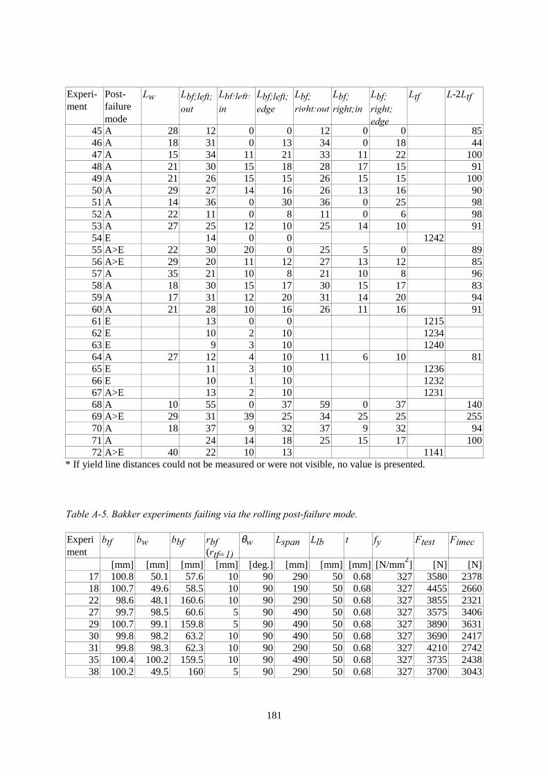
181
Experi-ment
Post-failuremode
Lw Lbf;left;out
Lbf;left;in
Lbf;left;edge
Lbf;right;out
Lbf;right;in
Lbf;right;edge
Ltf L-2Ltf
45 A 28 12 0 0 12 0 0 8546 A 18 31 0 13 34 0 18 4447 A 15 34 11 21 33 11 22 10048 A 21 30 15 18 28 17 15 9149 A 21 26 15 15 26 15 15 10050 A 29 27 14 16 26 13 16 9051 A 14 36 0 30 36 0 25 9852 A 22 11 0 8 11 0 6 9853 A 27 25 12 10 25 14 10 9154 E 14 0 0 124255 A>E 22 30 20 0 25 5 0 8956 A>E 29 20 11 12 27 13 12 8557 A 35 21 10 8 21 10 8 9658 A 18 30 15 17 30 15 17 8359 A 17 31 12 20 31 14 20 9460 A 21 28 10 16 26 11 16 9161 E 13 0 0 121562 E 10 2 10 123463 E 9 3 10 124064 A 27 12 4 10 11 6 10 8165 E 11 3 10 123666 E 10 1 10 123267 A>E 13 2 10 123168 A 10 55 0 37 59 0 37 14069 A>E 29 31 39 25 34 25 25 25570 A 18 37 9 32 37 9 32 9471 A 24 14 18 25 15 17 10072 A>E 40 22 10 13 1141
* If yield line distances could not be measured or were not visible, no value is presented.
Table A-5. Bakker experiments failing via the rolling post-failure mode.
Experiment
btf bw bbf rbf(rtf=1)
θw Lspan Llb t fy Ftest Fimec
[mm] [mm] [mm] [mm] [deg.] [mm] [mm] [mm] [N/mm2] [N] [N]17 100.8 50.1 57.6 10 90 290 50 0.68 327 3580 237818 100.7 49.6 58.5 10 90 190 50 0.68 327 4455 266022 98.6 48.1 160.6 10 90 290 50 0.68 327 3855 232127 99.7 98.5 60.6 5 90 490 50 0.68 327 3575 340629 100.7 99.1 159.8 5 90 490 50 0.68 327 3890 363130 99.8 98.2 63.2 10 90 490 50 0.68 327 3690 241731 99.8 98.3 62.3 10 90 290 50 0.68 327 4210 274235 100.4 100.2 159.5 10 90 490 50 0.68 327 3735 243838 100.2 49.5 160 5 90 290 50 0.68 327 3700 3043
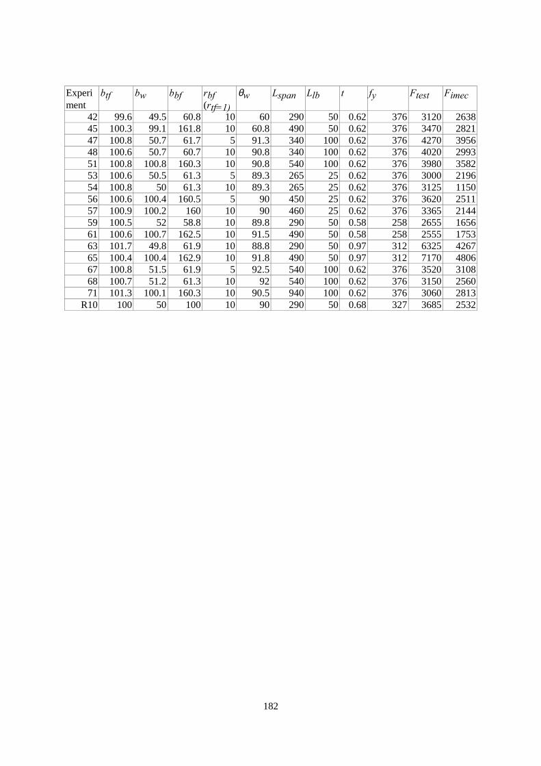
182
Experiment
btf bw bbf rbf(rtf=1)
θw Lspan Llb t fy Ftest Fimec
42 99.6 49.5 60.8 10 60 290 50 0.62 376 3120 263845 100.3 99.1 161.8 10 60.8 490 50 0.62 376 3470 282147 100.8 50.7 61.7 5 91.3 340 100 0.62 376 4270 395648 100.6 50.7 60.7 10 90.8 340 100 0.62 376 4020 299351 100.8 100.8 160.3 10 90.8 540 100 0.62 376 3980 358253 100.6 50.5 61.3 5 89.3 265 25 0.62 376 3000 219654 100.8 50 61.3 10 89.3 265 25 0.62 376 3125 115056 100.6 100.4 160.5 5 90 450 25 0.62 376 3620 251157 100.9 100.2 160 10 90 460 25 0.62 376 3365 214459 100.5 52 58.8 10 89.8 290 50 0.58 258 2655 165661 100.6 100.7 162.5 10 91.5 490 50 0.58 258 2555 175363 101.7 49.8 61.9 10 88.8 290 50 0.97 312 6325 426765 100.4 100.4 162.9 10 91.8 490 50 0.97 312 7170 480667 100.8 51.5 61.9 5 92.5 540 100 0.62 376 3520 310868 100.7 51.2 61.3 10 92 540 100 0.62 376 3150 256071 101.3 100.1 160.3 10 90.5 940 100 0.62 376 3060 2813
R10 100 50 100 10 90 290 50 0.68 327 3685 2532
183
Summary
Cold-formed trapezoidal sheeting of thin steel plate is a very popular product for buildingconstruction. It combines low weight and high strength and is economical in use. Currentdesign rules, which predict sheeting failure for an interior support, do not provide sufficientinsight into the sheeting behaviour, and can differ up to 40 % in their predictions. To developa new design rule, this thesis presents new experiments in which first-generation sheetingbehaviour is studied for practical situations. The experiments show that after ultimate load,three different post-failure modes arise. Mechanical models have been developed for the threepost-failure modes. These models can help to explain why a certain post-failure mode occurs.Finite element models were used to simulate the experiments. Studying stress distributionswith finite element simulations, it can be seen that there are only two ultimate failure modesat ultimate load. One of these ultimate failure modes is not relevant for practice. A mechanicalmodel has been developed for the other ultimate failure mode. This model performs as well asthe current design rules, and it provides insight into the sheeting behaviour.
Samenvatting
Koudgevormde, trapeziumvormige dakplaten, gemaakt van dunne staalplaat, wordenveelvuldig gebruikt in de bouwpraktijk. De platen zijn licht, goedkoop, en hebben een hogesterkte. De huidige ontwerpregels (die het bezwijken van de platen voorspellen) geven weiniginzicht in het gedrag van de platen. Bovendien lopen de voorspellingen van de diverseontwerpregels wel 40 % uiteen. Om betere ontwerpregels te ontwikkelen, worden in ditproefschrift nieuwe experimenten gepresenteerd. De experimenten laten zien dat voor platener drie manieren bestaan van gedrag na bezwijken. Voor de drie manieren van gedrag nabezwijken zijn mechanische modellen ontwikkeld. Deze modellen helpen te verklarenwaarom een specifieke manier van gedrag na bezwijken ontstaat. Eindige elementen modellenzijn gebruikt om de experimenten te simuleren. Door middel van spanningsverdelingen latenze zien dat voor platen er maar twee manieren van gedrag zijn tijdens bezwijken. Bovendienblijkt dat een van deze manieren van gedrag niet relevant is voor de praktijk. Voor de andere,relevante manier van gedrag is een mechanisch model ontwikkeld. Dit model is net zo goedals de huidige ontwerpregels, maar het geeft wel inzicht in het gedrag van de platen.
184
Curriculum Vitae
June 17, 1972 Born in Beek (Limburg), The Netherlands.
September 1, 1984 -August 31, 1989
Higher General Secondary Education "St.-Michiel", Geleen.
September 1, 1989 -August 31, 1990
Foundation course Architecture / Civil Engineering at HeerlenTechnical College (B.Sc. level).
September 1, 1990 -August 31, 1994
Architecture at the Technische Universiteit Eindhoven (M.Sc.level).
September 1, 1994 -April 30, 1995
Ph.D. student (Computer Aided Structural Design). This project wasterminated.
January 23, 1995 -March 31, 1995
Research fellow at the Institut für Baustatik, Universität Stuttgart,Germany.
May 1, 1995 -December 18, 2000
Ph.D. student (Combined Web Crippling and Bending MomentFailure of First-Generation Trapezoidal Steel Sheeting).
June 22, 1998 -September 20, 1998
Research fellow at the Physical Infrastructure Centre, QueenslandUniversity of Technology, Brisbane, Australia.


Report TUE-BCO-00-09
Report on Combined Web Crippling and Bending Moment Failure ofFirst-Generation Trapezoidal Steel Sheeting
Appendices to the thesis
H. Hofmeyer

ISBN 90-6814-115-5
© H. Hofmeyer, 2000
This research was supported by the Technology Foundation STW, applied science division ofNWO and the technology programme of the Ministry of Economic Affairs.
i
Contents
Notation ................................................................................................................................... iii
1 Appendix ultimate failure mechanical model ................................................................2
1.1 Beam on elastic foundation model ..............................................................................21.2 Marguerre's equations .................................................................................................51.3 Model equations ............................................................................................................81.4 Tomà and Stark experiments ....................................................................................111.5 Wing experiments .......................................................................................................121.6 Tsai experiments .........................................................................................................19
2 Appendix post-failure mechanical models ...................................................................20
2.1 Methodology................................................................................................................202.1.1 Prediction ultimate load........................................................................................202.1.2 Neglecting types of behaviour..............................................................................222.1.3 The principle of elastic and plastic components...................................................232.1.4 Corrections for method A .....................................................................................272.1.5 Mathematical techniques ......................................................................................29
2.2 Models for the yield arc post-failure mode ..............................................................332.2.1 Components: elastic behaviour.............................................................................332.2.2 Components: plastic behaviour for the yield arc post-failure mode.....................352.2.3 Prediction of the ultimate load using components................................................392.2.4 Overview of formulae...........................................................................................442.2.5 Other models.........................................................................................................45
2.3 Models for the rolling post-failure mode ..................................................................482.3.1 Components: plastic behaviour for the rolling post-failure mode........................482.3.2 Prediction of the ultimate load using components................................................492.3.3 Overview of formulae...........................................................................................512.3.4 Other models.........................................................................................................52
2.4 Model for the yield eye post-failure mode ................................................................552.4.1 Plastic component.................................................................................................552.4.2 Prediction of the ultimate load using components................................................56
2.5 Post-failure model results ..........................................................................................602.5.1 Verification methods ............................................................................................602.5.2 Verification of yield arc post-failure models........................................................612.5.3 Verification of rolling post-failure models ...........................................................622.5.4 Verification of yield eye post-failure model.........................................................63
2.6 Conclusions .................................................................................................................64
ii
3 Appendix detailed derivations post-failure models .....................................................65
3.1 Derivation of formulae 2.18 to 2.21...........................................................................653.2 Derivation of formulae 2.22, 2.23, and 2.24..............................................................663.3 Derivation of formulae 2.26, 2.27, 2.28, and 2.29.....................................................693.4 Derivation of formulae 2.69, 2.70, 2.71, 2.72, and 2.73............................................733.5 Derivation of formula 2.35 .........................................................................................793.6 Derivation of formulae 2.43 to 2.49...........................................................................833.7 Derivation of formula 2.53 .........................................................................................883.8 Derivation of formula 2.57 .........................................................................................893.9 Derivation of formulae 2.74 and 2.75........................................................................91
4 Appendix cross-section behaviour ................................................................................96
4.1 Introduction ................................................................................................................974.2 Finite element models ...............................................................................................1004.3 Mechanical models ...................................................................................................105
4.3.1 Location of first yield line ..................................................................................1054.3.2 Plastic behaviour.................................................................................................110
4.4 Discussion ..................................................................................................................1144.4.1 Difference for small and large corner radii ........................................................1144.4.2 Comparison of strips and whole sheet sections using finite element models.....114
4.5 Conclusions ...............................................................................................................116
5 Appendix Turbo Pascal programs ..............................................................................117
5.1 Program for Eurocode3 predictions .......................................................................1175.2 Program for ultimate failure mechanical model ...................................................1265.3 Program for post-failure mechanical model MA1.................................................1325.4 Program for post-failure mechanical model MR1.................................................1375.5 Program for post-failure mechanical model ME1.................................................140
6 Input files for Ansys 5.4 ...............................................................................................142
6.1 Input file for yield arc finite element model (experiment 36)...............................1426.2 Input file for rolling finite element model (experiment 54 Bakker).....................1556.3 Input file for yield eye finite element model (experiment 40)...............................165
Literature ..............................................................................................................................179
iii
Notation
General variables
F Actual concentrated load, can be in combination with bending moment [N].k Stiffness between concentrated load and web crippling deformation [N/mm].M Actual bending moment, can be in combination with concentrated load [Nmm].Mu Ultimate bending moment if there is no concentrated load [Nmm].∆hw Web crippling deformation. The reduction of height hw [mm].∆ ... Difference of ...δ ... Incremental ...
Sheeting variables (see also thesis [Hofm00a], chapter 2, figure 2-3)
bbf Bottom flange width [mm].bbffl Flat bottom flange width [mm].bm Total width between top flange middles [mm].btf Top flange width [mm].btffl Flat top flange width [mm].bw Web width [mm].bwfl Flat web width [mm].E Modulus of elasticity [N/mm2].fy Steel yield strength [N/mm2].hm Sheeting height as shown in figure 2-3, chapter 2, thesis [Hofm00a] [mm].hw Sheeting height as shown in figure 2-3, chapter 2, thesis [Hofm00a] [mm].Llb Load-bearing plate width [mm].Lspan Span length [mm].rbf Radius of bottom corner [mm].ribf Interior radius of bottom corner [mm].ritf Interior radius of top corner [mm].rtf Radius of top corner [mm].t Steel plate thickness [mm].θw Angle between web and flange [deg.].
Yield line distances
Lbf;left;edgeLbf;right;edge
Distance between left / right two yield lines in bottom flange at the bottom corner[mm].
Lbf;left;inLbf;right;in
Distance between load-bearing plate and inner left / right yield line in bottomflange [mm].
Lbf;left;outLbf;right;out
Distance between load-bearing plate and outer left / right yield line in bottomflange [mm].
Ltf Distance between support and yield line in top flange [mm].Lw Distance between bottom corner and yield line in web [mm].Lyb Distance between yield lines in bottom flange (Bakker's model) [mm].Lyt Distance between yield lines in top flange (Bakker's model) [mm].
iv
Appendix 1 (ultimate failure mechanical model)
b Substitute variable for beam on elastic foundation model.b, L Width and length of plate for Marguerre's equations [mm].dQ, dP Distances of point Q and P to line of intersection top flange and web [mm].dx Infinite small piece of sheeting in length direction.E Modulus of elasticity [N/mm2].F Actual concentrated load [N].f1 Function.Fmin, Fmax Minimum and maximum values for the estimation of load F [N].Ftest Ultimate load Fu measured during an experiment.I Moment of inertia for sheeting longitudinal section for sheeting part above the
load-bearing plate [mm4].Is Moment of inertia for total sheeting cross-section [mm4].k Stiffness between concentrated load and web crippling deformation [N/mm].K1, K2 Factors in Marguerre's equations.M Actual bending moment, can be in combination with concentrated load [Nmm].Ma Bending moment in sheeting part above the load-bearing plate [Nmm].P, Q, R, S, T Points on the bottom flange.q Equally distributed load [N/mm2].Rh Reaction force for sheeting part above the load-bearing plate [N].u, w, v Displacements along the x, y, and z-axis (should not be u, v, w, which seems to be
more logical, see figure 1-3).w0 Out-of-plane displacement of modelled part bottom flange [mm].wa Deflection of point a [mm], used in the beam on elastic foundation model.wmin, wmax Minimum and maximum values for the estimation of displacement w0 [mm].wP, wR, wS Out-of-plane displacements of point P, R, and S [mm].x, y, z Variables defining coordinate system.y0 Initial imperfection of midpoint in modelled part of bottom flange [mm].zp Distance between centre of gravity and bottom flange [mm].∆hw Web crippling deformation. The reduction of height hw [mm].α Part of the web, used in the beam on elastic foundation model.α, β Substitution variables for Marguerre's equations [mm].λ, C1, C2, C3,D, p
Substitution variables.
ν Poisson constant (0.3).σVM Von Mises stress [N/mm2].σx max ,z max Normal stresses in the outer fibres caused by bending moment in direction of x/z-
axis [N/mm2].σx,z Normal stress in direction of x / z axis [N/mm2].σz Compressive stress in bottom flange [N/mm2].τxz Shear stress in plane perpendicular to the x-axis, in z-direction [N/mm2].
Appendix 2 and 3 (post-failure mechanical models)
e Main value for experimental values for the ultimate load.m Main value for model predictions of the ultimate load.

v
{A, B, C, D, E,F, G, H, I, J,K}
Set of factors to simplify formulae.
a Length of yield eye / flip disc [mm].A, B, C Constants.A, B, C, D, E Parameters to illustrate mathematical techniques.a, b, c, d, e, f Constants to illustrate mathematical techniques.Aw ,Af , At Web / flange / total area for U-section [mm2].b Substitute variable for calculation Fe.b Width of yield eye / flip disc [mm].b1, b2, b3 Distances in figure 3-5 to determine relationship ∆hw and ϕc.c1 Substitution variable.d1, d2, d3 Differences between predicted loads [N].ei Experiment i.f, g, h, i Functions to illustrate mathematical techniques.F2p Load to deform two parts adjacent to the load-bearing plate [N].Fbf Normal force in the bottom flange [N].Fcs Load to deform cross-section [N].Fcsu Ultimate load of cross-section [N].Fe Load to deform cross-section elastically [N].Fl Extra force due to the indentation of the cross-section [N].fl1,2 Length factor 1, 2.Fp Load to deform cross-section plastically [N].Fylbf Load to form yield lines in the bottom flange [N].h U-section height [mm].h Sheeting height to illustrate web crippling stiffness in figure 2-13 [mm].Is Moment of inertia for complete sheeting cross-section [mm4].Lbf Abbreviation for Lbf;left;out.Li Length yield line i.Lyw Specific yield line length in figure 3-2.Mi,e Internal / external bending moment [Nmm].n Number of experiments.Pi Point i.s Distance of bottom flange to centre of gravity sheet section [mm].se,m Standard deviation for experiments / model predictions.u Deformation of U-section [mm].u1, F1 A specific deformation / force value of the U-section [mm].u4;fl,w Horizontal / vertical displacement of point P4 [mm].ua, ub Movements of yield lines in the cross-section [mm].wtf Distance between yield lines as shown in figure 3-2 [mm].x, y, z Variables to illustrate mathematical techniques.x, α, β Substituting variables.∆ Out-of-plane deflection yield eye / flip disc [mm].∆bwfl Reduction of distance bwfl [mm].δEe Incremental external energy.δEe1 Incremental external energy cross-section only.δEe2 Incremental external energy cross-section and sheet section deflection.δEi Incremental internal dissipated energy.
vi
φ Substitution variableϕ Support rotation [rad.].ϕi Rotation of yield line i [rad.]ϕit, ϕ∆ Specific yield line angles (no rotations) used in figure 3-1.ϕw Rotation around point P1 for line P1-P4 [rad.].ρ Standard deviation for experiments.
Appendix 4 (cross-section behaviour)
d, w, h Distances [mm] in cross-section figure 4-10.d1, d2 Distances as defined in figure 4-11 [mm].dx Infinite small piece of sheeting in length direction.dy Movement of yield line in web [mm].h1, h2 Variables to illustrate the web crippling deformation ∆hw [mm].Hs Horizontal load [N].Ly Distance from top web to yield line in web [mm].Mi,s Bending moment i, s [N].Mpl Plastic bending moment [Nmm].P Axial load in the web [N].Pcr The buckling load of the web [N].rotx, roty, rotz Rotations around the x-, y-, and z-axes.u1, u2 Movement of upper and lower part cross-section as shown in figure 4-11 [mm].ux, uy, uz Displacements along the x-, y-, and z-axes.Vs Vertical load [N].α, β Variables for local coordinate system in cross-section (figure 4-10).φ, ψ Functions by Timoshenko.η Substitution variable.ϕI Rotation at location I.

1
Introduction
In this report, six appendices are presented. These appendices are meant to be used with thethesis [Hofm00a].
The first appendix presents the model of thesis chapter 5 a little more extendedly. Appendix 2shows a detailed description of the post-failure models, as presented in chapter 6 of the thesis.The third appendix is used to present all derivations too tedious to present in appendix 2.Finally, appendix 4 shows pure cross-section behaviour for sheeting, using finite elementsimulations and mechanical models.
Appendix 5 and 6 present several listings of Turbo Pascal programs and input files for thefinite element program Ansys 5.4.
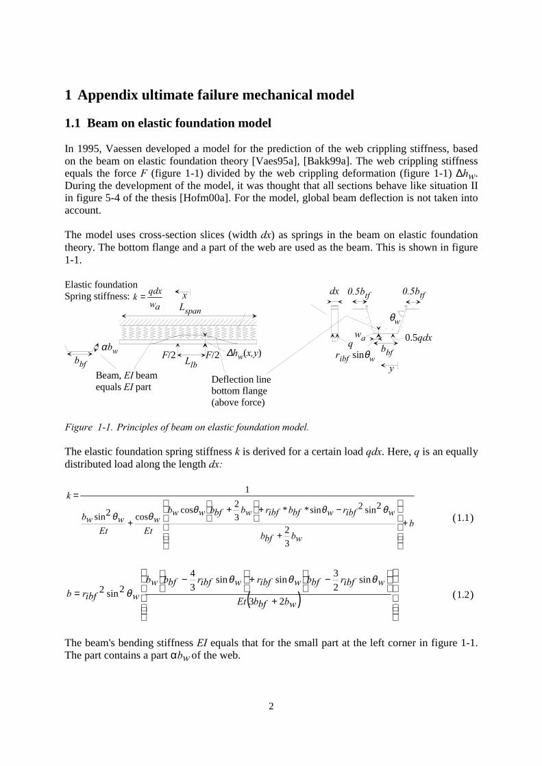
2
1 Appendix ultimate failure mechanical model
1.1 Beam on elastic foundation model
In 1995, Vaessen developed a model for the prediction of the web crippling stiffness, basedon the beam on elastic foundation theory [Vaes95a], [Bakk99a]. The web crippling stiffnessequals the force F (figure 1-1) divided by the web crippling deformation (figure 1-1) ∆hw.During the development of the model, it was thought that all sections behave like situation IIin figure 5-4 of the thesis [Hofm00a]. For the model, global beam deflection is not taken intoaccount.
The model uses cross-section slices (width dx) as springs in the beam on elastic foundationtheory. The bottom flange and a part of the web are used as the beam. This is shown in figure1-1.
Elastic foundationSpring stiffness:
Beam, EI beamequals EI part
F/2F/2 Llb
Lspan
bbf
0.5btf0.5btf
θwwa 0.5qdxq
dx
bbf
αbw ribf sinθw
Deflection linebottom flange(above force)
∆hw(x,y)
x
y
awqdxk =
Figure 1-1. Principles of beam on elastic foundation model.
The elastic foundation spring stiffness k is derived for a certain load qdx. Here, q is an equallydistributed load along the length dx:
bwbbfb
wibfrwbfbibfrwbbfbwwb
Etw
Etwwb
k
+
+
−+
+
+
=
32
2sin2sin**32cos
cos2sin
1
θθθθθ (1.1)
( )
+
−+
−
=wbbfbEt
wibfrbfbwibfrwibfrbfbwbwibfrb
23
sin23sinsin
34
2sin2θθθ
θ (1.2)
The beam's bending stiffness EI equals that for the small part at the left corner in figure 1-1.The part contains a part αbw of the web.
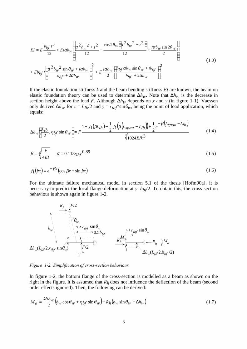
3
2
2
sin
2
2
2sin22
22sin
12
2222cos
12
222
12
3
+
++
++
+
+
−−
++=
wbbfbbftbwwbbfbwbt
Ewbbfb
wbtwwbtbfEb
wwbttwbwtwbwbEt
tbfbEEI
α
θααα
αθα
θααθαα
(1.3)
If the elastic foundation stiffness k and the beam bending stiffness EI are known, the beam onelastic foundation theory can be used to determine ∆hw. Note that ∆hw is the decrease insection height above the load F. Although ∆hw depends on x and y (in figure 1-1), Vaessenonly derived ∆hw for x = Llb/2 and y = ribf*sinθw, being the point of load application, whichequals:
( ) ( )( ) ( )4 31024
21
121
11sin,
2 EIk
lbLspanLelbLspanLflbLf
FwibfrlbLwh
−−+−−+
=
∆
βββ
θ (1.4)
44EI
k=β
89.0118.0 ibfr=α (1.5)
( ) ( )xxxexf ββββ sincos1 +−= (1.6)
For the ultimate failure mechanical model in section 5.1 of the thesis [Hofm00a], it isnecessary to predict the local flange deformation at y=bbf/2. To obtain this, the cross-sectionbehaviour is shown again in figure 1-2.
F/2Rh
θwribf sinθw
0.5bbfbw
F/2
MaRh
y
y+ribf sinθw
∆hw(Llb/2,ribf sinθw)∆hw(Llb/2,bbf /2)
MaRh
Figure 1-2. Simplification of cross-section behaviour.
In figure 1-2, the bottom flange of the cross-section is modelled as a beam as shown on theright in the figure. It is assumed that Rh does not influence the deflection of the beam (secondorder effects ignored). Then, the following can be derived:
( ) ( )whwwbhRwibfrwwbwhkaM ∆−−+
∆= θθθ sinsincos
2(1.7)
4
EI
wibfrbfbaM
wibfrlbLwhbfblbL
wh2
2sin
2sin,
22,
2
−
+
∆=
∆
θθ
(1.8)
+
−++∆=
wbbfb
wibfrwwbbfbwbfbibfrwwb
wwbwhk
hR
31
21
2sin2cossincos232
sin4
θθθθ
θ (1.9)
The latter formula was derived by Vaessen. This appendix can be summarised as follows. Fora sheet section, loaded by a load-bearing plate, the displacement of the bottom corner relativeto the upper corner can be calculated (web crippling deformation ∆hw(Llb/2,ribf*sinθw) anddQ in section 5.1.2 of the thesis [Hofm00a]). If this deformation is known, the displacementof the bottom flange middle relative to the bottom corner can be predicted (∆hw(Llb/2,bbf/2)and dP in section 5.1.2 of the thesis [Hofm00a]).
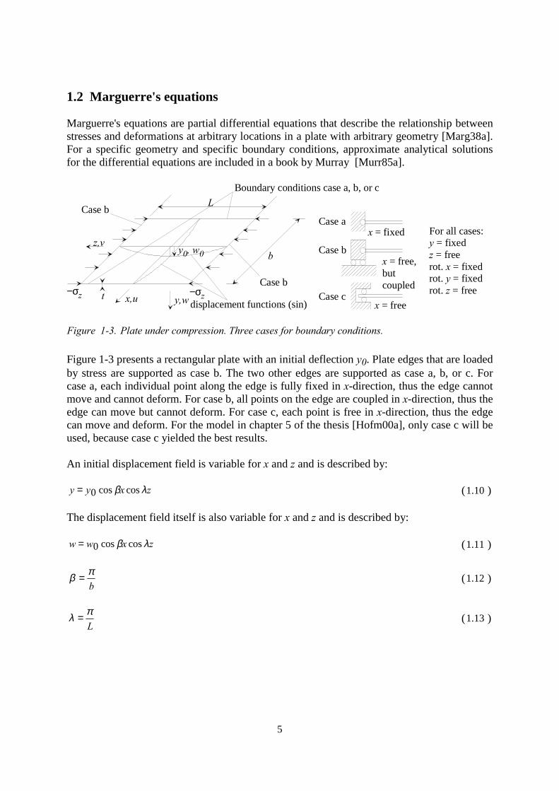
5
1.2 Marguerre's equations
Marguerre's equations are partial differential equations that describe the relationship betweenstresses and deformations at arbitrary locations in a plate with arbitrary geometry [Marg38a].For a specific geometry and specific boundary conditions, approximate analytical solutionsfor the differential equations are included in a book by Murray [Murr85a].
x,u y,w
z,v
t
L
b
−σz −σz
y0, w0
displacement functions (sin)
Boundary conditions case a, b, or c
Case a
Case b
Case c
x = free,butcoupled
x = free
x = fixed
Case b
Case b
For all cases:y = fixedz = freerot. x = fixedrot. y = fixedrot. z = free
Figure 1-3. Plate under compression. Three cases for boundary conditions.
Figure 1-3 presents a rectangular plate with an initial deflection y0. Plate edges that are loadedby stress are supported as case b. The two other edges are supported as case a, b, or c. Forcase a, each individual point along the edge is fully fixed in x-direction, thus the edge cannotmove and cannot deform. For case b, all points on the edge are coupled in x-direction, thus theedge can move but cannot deform. For case c, each point is free in x-direction, thus the edgecan move and deform. For the model in chapter 5 of the thesis [Hofm00a], only case c will beused, because case c yielded the best results.
An initial displacement field is variable for x and z and is described by:
zxyy λβ coscos0= (1.10 )
The displacement field itself is also variable for x and z and is described by:
zxww λβ coscos0= (1.11 )
bπβ = (1.12 )
Lπλ = (1.13 )
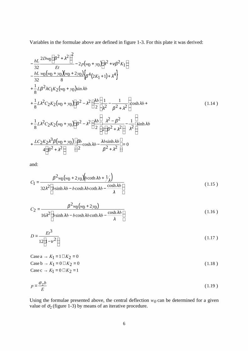
6
Variables in the formulae above are defined in figure 1-3. For this plate it was derived:
( )( )( ) ( ){ }
( )
( )
( )
( ) 022sinhcosh
222400
322
sinh21
222
22
222
00222
81
cosh221
21
222
00222
81
sin00212
81
411248
02000032
122
002
22202
32
=
+−
+
++
−
+
−
−++
+
+−
−++
++
++++−
++−
+−
λβ
λλλβ
λβ
βλ
λλλβ
βλλλβλ
λλβλ
λλβλ
λλβ
λβ
νβλλβ
bbbbywKLC
bbywKCL
bbywKCL
bywKCL
KywywwbL
KywpEt
DwbL
(1.14 )
and:
( )( )
−−
++=
λλλλλλ
λλβbbbbbb
bbywwC
coshcothcoshsinh232
1coth02002
1 (1.15 )
( )
−−
+=
λλλλλλ
βbbbbbb
ywwCcoshcothcoshsinh216
02002
2 (1.16 )
−=
2112
3
ν
EtD (1.17 )
1201c Case0201b Case0211a Case
=∧=→=∧=→=∧=→
KKKKKK
(1.18 )
Ebzp σ= (1.19 )
Using the formulae presented above, the central deflection w0 can be determined for a givenvalue of σz (figure 1-3) by means of an iterative procedure.
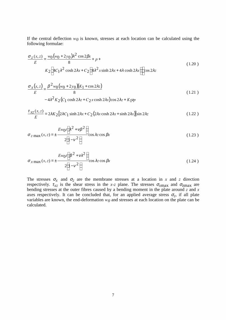
7
If the central deflection w0 is known, stresses at each location can be calculated using thefollowing formulae:
( )
zxxxCxCK
pxyww
Ezxz
λλλλλλλ
βλσ
2cos2cosh42sinh2422cosh2142
82cos2
0200),(
++
+++
=(1.20 )
( ) ( )( )
( ) pKzxxCzCK
zKywwE
zxx
νλλλλ
λβσ
12cos2cosh22cosh1224
82cos10200
2,
++−
++=
(1.21 )
( )[ ] zxxxCxCKE
zxxz λλλλλλλτ
2sin2sinh2cosh222sinh1222),(
++= (1.22 )
xztEw
zxz βλν
νβλσ coscos
212
220
),(max
−
+±= (1.23 )
xztEw
zxx βλν
νλβσ coscos
212
220
),(max
−
+±= (1.24 )
The stresses σx and σz are the membrane stresses at a location in x and z directionrespectively. τxz is the shear stress in the x-z plane. The stresses σxmax and σzmax arebending stresses at the outer fibres caused by a bending moment in the plate around z and xaxes respectively. It can be concluded that, for an applied average stress σz, if all platevariables are known, the end-deformation w0 and stresses at each location on the plate can becalculated.
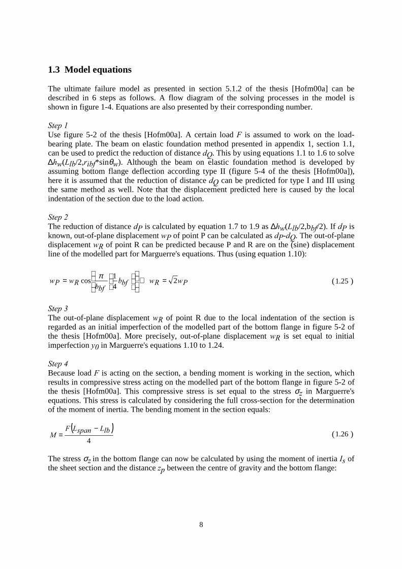
8
1.3 Model equations
The ultimate failure model as presented in section 5.1.2 of the thesis [Hofm00a] can bedescribed in 6 steps as follows. A flow diagram of the solving processes in the model isshown in figure 1-4. Equations are also presented by their corresponding number.
Step 1Use figure 5-2 of the thesis [Hofm00a]. A certain load F is assumed to work on the load-bearing plate. The beam on elastic foundation method presented in appendix 1, section 1.1,can be used to predict the reduction of distance dQ. This by using equations 1.1 to 1.6 to solve∆hw(Llb/2,ribf*sinθw). Although the beam on elastic foundation method is developed byassuming bottom flange deflection according type II (figure 5-4 of the thesis [Hofm00a]),here it is assumed that the reduction of distance dQ can be predicted for type I and III usingthe same method as well. Note that the displacement predicted here is caused by the localindentation of the section due to the load action.
Step 2The reduction of distance dP is calculated by equation 1.7 to 1.9 as ∆hw(Llb/2,bbf/2). If dP isknown, out-of-plane displacement wP of point P can be calculated as dP-dQ. The out-of-planedisplacement wR of point R can be predicted because P and R are on the (sine) displacementline of the modelled part for Marguerre's equations. Thus (using equation 1.10):
PwRwbfbbfbRwPw 2
41cos =⇔
= π (1.25 )
Step 3The out-of-plane displacement wR of point R due to the local indentation of the section isregarded as an initial imperfection of the modelled part of the bottom flange in figure 5-2 ofthe thesis [Hofm00a]. More precisely, out-of-plane displacement wR is set equal to initialimperfection y0 in Marguerre's equations 1.10 to 1.24.
Step 4Because load F is acting on the section, a bending moment is working in the section, whichresults in compressive stress acting on the modelled part of the bottom flange in figure 5-2 ofthe thesis [Hofm00a]. This compressive stress is set equal to the stress σz in Marguerre'sequations. This stress is calculated by considering the full cross-section for the determinationof the moment of inertia. The bending moment in the section equals:
( )4
lbLspanLFM
−= (1.26 )
The stress σz in the bottom flange can now be calculated by using the moment of inertia Is ofthe sheet section and the distance zp between the centre of gravity and the bottom flange:
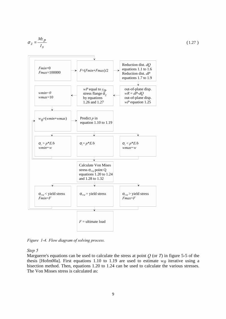
9
sIpMz
z =σ (1.27 )
Fmin=0Fmax=100000
Reduction dist. dQequations 1.1 to 1.6Reduction dist. dPequations 1.7 to 1.9
F=(Fmin+Fmax)/2
wP equal to y0,
Calculate Von Misesstress σVM point Qequations 1.20 to 1.24and 1.28 to 1.32
σVM < yield stressFmin=F
σVM > yield stressFmax=F
σVM = yield stress
F = ultimate load
wmin=0wmax=10
w0=(wmin+wmax) Predict p inequation 1.10 to 1.19
σz < p*E/bwmax=w
σz > p*E/bwmin=w
σz= p*E/b
out-of-plane disp.wR = dP-dQout-of-plane disp.wP equation 1.25
stress flange σz by equations1.26 and 1.27
Figure 1-4. Flow diagram of solving process.
Step 5Marguerre's equations can be used to calculate the stress at point Q (or T) in figure 5-5 of thethesis [Hofm00a]. First equations 1.10 to 1.19 are used to estimate w0 iterative using abisection method. Then, equations 1.20 to 1.24 can be used to calculate the various stresses.The Von Misses stress is calculated as:

10
( ) ( )( )( ) xzyyzz
yyzzVMτσσσσ
σσσσσ
3maxmax2
2max
2max
21
+++
−+++=(1.28 )
( ) ( )( )( ) xzyyzz
yyzzVMτσσσσ
σσσσσ
3maxmax2
2max
2max
22
+−−
−−+−=(1.29 )
( )2,1max VMVMVM σσσ = (1.30 )
bbflbx21= (1.31 )
bfflbz41= for point Q and 0=z for point T (1.32 )
Step 6If this stress σVM is lower than the yield stress, a higher load F should be tried and vice versa.This iterative process is carried out using a bisection method. If the stress at Q (or T) equalsthe yield stress, the load F is regarded as the ultimate load.
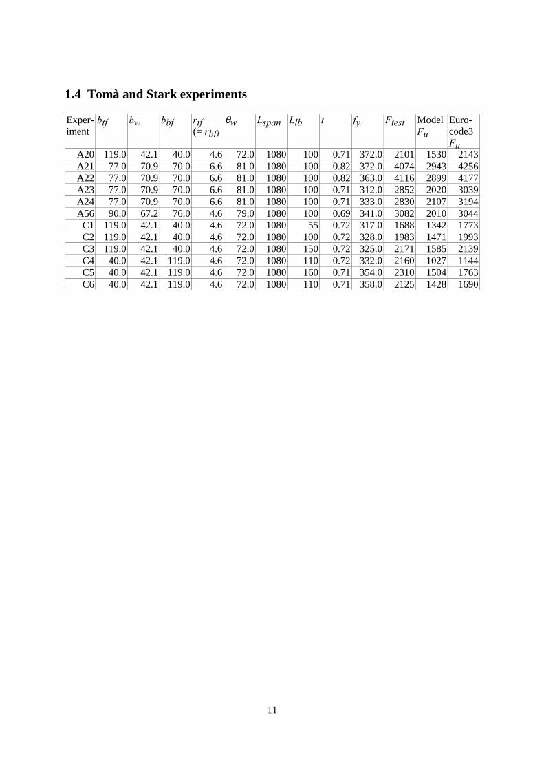
11
1.4 Tomà and Stark experiments
Exper-iment
btf bw bbf rtf(= rbf)
θw Lspan Llb t fy Ftest ModelFu
Euro-code3Fu
A20 119.0 42.1 40.0 4.6 72.0 1080 100 0.71 372.0 2101 1530 2143A21 77.0 70.9 70.0 6.6 81.0 1080 100 0.82 372.0 4074 2943 4256A22 77.0 70.9 70.0 6.6 81.0 1080 100 0.82 363.0 4116 2899 4177A23 77.0 70.9 70.0 6.6 81.0 1080 100 0.71 312.0 2852 2020 3039A24 77.0 70.9 70.0 6.6 81.0 1080 100 0.71 333.0 2830 2107 3194A56 90.0 67.2 76.0 4.6 79.0 1080 100 0.69 341.0 3082 2010 3044
C1 119.0 42.1 40.0 4.6 72.0 1080 55 0.72 317.0 1688 1342 1773C2 119.0 42.1 40.0 4.6 72.0 1080 100 0.72 328.0 1983 1471 1993C3 119.0 42.1 40.0 4.6 72.0 1080 150 0.72 325.0 2171 1585 2139C4 40.0 42.1 119.0 4.6 72.0 1080 110 0.72 332.0 2160 1027 1144C5 40.0 42.1 119.0 4.6 72.0 1080 160 0.71 354.0 2310 1504 1763C6 40.0 42.1 119.0 4.6 72.0 1080 110 0.71 358.0 2125 1428 1690
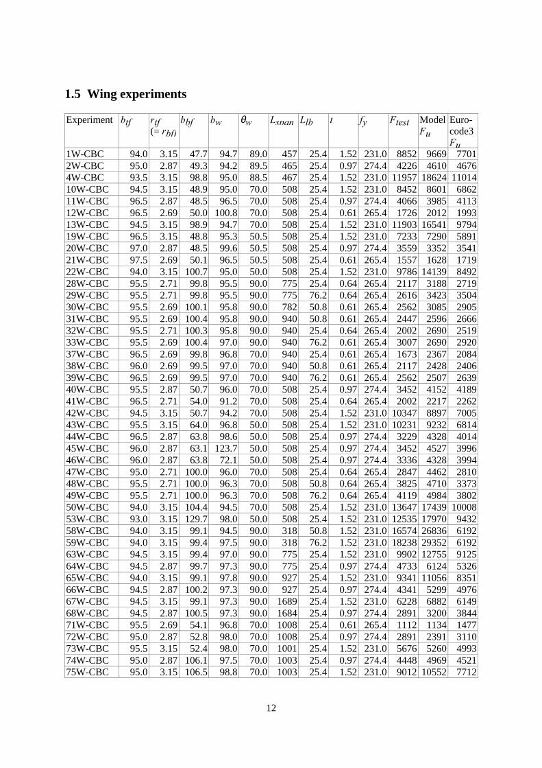
12
1.5 Wing experiments
Experiment btf rtf(= rbf)
bbf bw θw Lspan Llb t fy Ftest ModelFu
Euro-code3Fu
1W-CBC 94.0 3.15 47.7 94.7 89.0 457 25.4 1.52 231.0 8852 9669 77012W-CBC 95.0 2.87 49.3 94.2 89.5 465 25.4 0.97 274.4 4226 4610 46764W-CBC 93.5 3.15 98.8 95.0 88.5 467 25.4 1.52 231.0 11957 18624 1101410W-CBC 94.5 3.15 48.9 95.0 70.0 508 25.4 1.52 231.0 8452 8601 686211W-CBC 96.5 2.87 48.5 96.5 70.0 508 25.4 0.97 274.4 4066 3985 411312W-CBC 96.5 2.69 50.0 100.8 70.0 508 25.4 0.61 265.4 1726 2012 199313W-CBC 94.5 3.15 98.9 94.7 70.0 508 25.4 1.52 231.0 11903 16541 979419W-CBC 96.5 3.15 48.8 95.3 50.5 508 25.4 1.52 231.0 7233 7290 589120W-CBC 97.0 2.87 48.5 99.6 50.5 508 25.4 0.97 274.4 3559 3352 354121W-CBC 97.5 2.69 50.1 96.5 50.5 508 25.4 0.61 265.4 1557 1628 171922W-CBC 94.0 3.15 100.7 95.0 50.0 508 25.4 1.52 231.0 9786 14139 849228W-CBC 95.5 2.71 99.8 95.5 90.0 775 25.4 0.64 265.4 2117 3188 271929W-CBC 95.5 2.71 99.8 95.5 90.0 775 76.2 0.64 265.4 2616 3423 350430W-CBC 95.5 2.69 100.1 95.8 90.0 782 50.8 0.61 265.4 2562 3085 290531W-CBC 95.5 2.69 100.4 95.8 90.0 940 50.8 0.61 265.4 2447 2596 266632W-CBC 95.5 2.71 100.3 95.8 90.0 940 25.4 0.64 265.4 2002 2690 251933W-CBC 95.5 2.69 100.4 97.0 90.0 940 76.2 0.61 265.4 3007 2690 292037W-CBC 96.5 2.69 99.8 96.8 70.0 940 25.4 0.61 265.4 1673 2367 208438W-CBC 96.0 2.69 99.5 97.0 70.0 940 50.8 0.61 265.4 2117 2428 240639W-CBC 96.5 2.69 99.5 97.0 70.0 940 76.2 0.61 265.4 2562 2507 263940W-CBC 95.5 2.87 50.7 96.0 70.0 508 25.4 0.97 274.4 3452 4152 418941W-CBC 96.5 2.71 54.0 91.2 70.0 508 25.4 0.64 265.4 2002 2217 226242W-CBC 94.5 3.15 50.7 94.2 70.0 508 25.4 1.52 231.0 10347 8897 700543W-CBC 95.5 3.15 64.0 96.8 50.0 508 25.4 1.52 231.0 10231 9232 681444W-CBC 96.5 2.87 63.8 98.6 50.0 508 25.4 0.97 274.4 3229 4328 401445W-CBC 96.0 2.87 63.1 123.7 50.0 508 25.4 0.97 274.4 3452 4527 399646W-CBC 96.0 2.87 63.8 72.1 50.0 508 25.4 0.97 274.4 3336 4328 399447W-CBC 95.0 2.71 100.0 96.0 70.0 508 25.4 0.64 265.4 2847 4462 281048W-CBC 95.5 2.71 100.0 96.3 70.0 508 50.8 0.64 265.4 3825 4710 337349W-CBC 95.5 2.71 100.0 96.3 70.0 508 76.2 0.64 265.4 4119 4984 380250W-CBC 94.0 3.15 104.4 94.5 70.0 508 25.4 1.52 231.0 13647 17439 1000853W-CBC 93.0 3.15 129.7 98.0 50.0 508 25.4 1.52 231.0 12535 17970 943258W-CBC 94.0 3.15 99.1 94.5 90.0 318 50.8 1.52 231.0 16574 26836 619259W-CBC 94.0 3.15 99.4 97.5 90.0 318 76.2 1.52 231.0 18238 29352 619263W-CBC 94.5 3.15 99.4 97.0 90.0 775 25.4 1.52 231.0 9902 12755 912564W-CBC 94.5 2.87 99.7 97.3 90.0 775 25.4 0.97 274.4 4733 6124 532665W-CBC 94.0 3.15 99.1 97.8 90.0 927 25.4 1.52 231.0 9341 11056 835166W-CBC 94.5 2.87 100.2 97.3 90.0 927 25.4 0.97 274.4 4341 5299 497667W-CBC 94.5 3.15 99.1 97.3 90.0 1689 25.4 1.52 231.0 6228 6882 614968W-CBC 94.5 2.87 100.5 97.3 90.0 1684 25.4 0.97 274.4 2891 3200 384471W-CBC 95.5 2.69 54.1 96.8 70.0 1008 25.4 0.61 265.4 1112 1134 147772W-CBC 95.0 2.87 52.8 98.0 70.0 1008 25.4 0.97 274.4 2891 2391 311073W-CBC 95.5 3.15 52.4 98.0 70.0 1001 25.4 1.52 231.0 5676 5260 499374W-CBC 95.0 2.87 106.1 97.5 70.0 1003 25.4 0.97 274.4 4448 4969 452175W-CBC 95.0 3.15 106.5 98.8 70.0 1003 25.4 1.52 231.0 9012 10552 7712
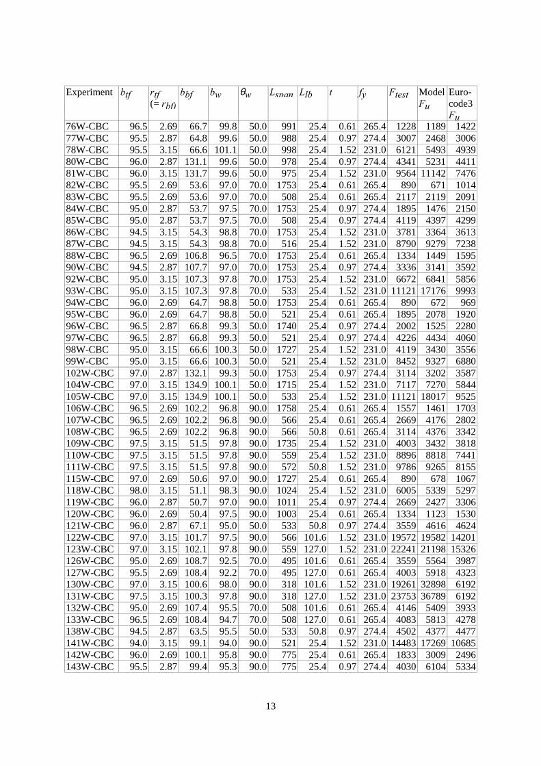
13
Experiment btf rtf(= rbf)
bbf bw θw Lspan Llb t fy Ftest ModelFu
Euro-code3Fu
76W-CBC 96.5 2.69 66.7 99.8 50.0 991 25.4 0.61 265.4 1228 1189 142277W-CBC 95.5 2.87 64.8 99.6 50.0 988 25.4 0.97 274.4 3007 2468 300678W-CBC 95.5 3.15 66.6 101.1 50.0 998 25.4 1.52 231.0 6121 5493 493980W-CBC 96.0 2.87 131.1 99.6 50.0 978 25.4 0.97 274.4 4341 5231 441181W-CBC 96.0 3.15 131.7 99.6 50.0 975 25.4 1.52 231.0 9564 11142 747682W-CBC 95.5 2.69 53.6 97.0 70.0 1753 25.4 0.61 265.4 890 671 101483W-CBC 95.5 2.69 53.6 97.0 70.0 508 25.4 0.61 265.4 2117 2119 209184W-CBC 95.0 2.87 53.7 97.5 70.0 1753 25.4 0.97 274.4 1895 1476 215085W-CBC 95.0 2.87 53.7 97.5 70.0 508 25.4 0.97 274.4 4119 4397 429986W-CBC 94.5 3.15 54.3 98.8 70.0 1753 25.4 1.52 231.0 3781 3364 361387W-CBC 94.5 3.15 54.3 98.8 70.0 516 25.4 1.52 231.0 8790 9279 723888W-CBC 96.5 2.69 106.8 96.5 70.0 1753 25.4 0.61 265.4 1334 1449 159590W-CBC 94.5 2.87 107.7 97.0 70.0 1753 25.4 0.97 274.4 3336 3141 359292W-CBC 95.0 3.15 107.3 97.8 70.0 1753 25.4 1.52 231.0 6672 6841 585693W-CBC 95.0 3.15 107.3 97.8 70.0 533 25.4 1.52 231.0 11121 17176 999394W-CBC 96.0 2.69 64.7 98.8 50.0 1753 25.4 0.61 265.4 890 672 96995W-CBC 96.0 2.69 64.7 98.8 50.0 521 25.4 0.61 265.4 1895 2078 192096W-CBC 96.5 2.87 66.8 99.3 50.0 1740 25.4 0.97 274.4 2002 1525 228097W-CBC 96.5 2.87 66.8 99.3 50.0 521 25.4 0.97 274.4 4226 4434 406098W-CBC 95.0 3.15 66.6 100.3 50.0 1727 25.4 1.52 231.0 4119 3430 355699W-CBC 95.0 3.15 66.6 100.3 50.0 521 25.4 1.52 231.0 8452 9327 6880102W-CBC 97.0 2.87 132.1 99.3 50.0 1753 25.4 0.97 274.4 3114 3202 3587104W-CBC 97.0 3.15 134.9 100.1 50.0 1715 25.4 1.52 231.0 7117 7270 5844105W-CBC 97.0 3.15 134.9 100.1 50.0 533 25.4 1.52 231.0 11121 18017 9525106W-CBC 96.5 2.69 102.2 96.8 90.0 1758 25.4 0.61 265.4 1557 1461 1703107W-CBC 96.5 2.69 102.2 96.8 90.0 566 25.4 0.61 265.4 2669 4176 2802108W-CBC 96.5 2.69 102.2 96.8 90.0 566 50.8 0.61 265.4 3114 4376 3342109W-CBC 97.5 3.15 51.5 97.8 90.0 1735 25.4 1.52 231.0 4003 3432 3818110W-CBC 97.5 3.15 51.5 97.8 90.0 559 25.4 1.52 231.0 8896 8818 7441111W-CBC 97.5 3.15 51.5 97.8 90.0 572 50.8 1.52 231.0 9786 9265 8155115W-CBC 97.0 2.69 50.6 97.0 90.0 1727 25.4 0.61 265.4 890 678 1067118W-CBC 98.0 3.15 51.1 98.3 90.0 1024 25.4 1.52 231.0 6005 5339 5297119W-CBC 96.0 2.87 50.7 97.0 90.0 1011 25.4 0.97 274.4 2669 2427 3306120W-CBC 96.0 2.69 50.4 97.5 90.0 1003 25.4 0.61 265.4 1334 1123 1530121W-CBC 96.0 2.87 67.1 95.0 50.0 533 50.8 0.97 274.4 3559 4616 4624122W-CBC 97.0 3.15 101.7 97.5 90.0 566 101.6 1.52 231.0 19572 19582 14201123W-CBC 97.0 3.15 102.1 97.8 90.0 559 127.0 1.52 231.0 22241 21198 15326126W-CBC 95.0 2.69 108.7 92.5 70.0 495 101.6 0.61 265.4 3559 5564 3987127W-CBC 95.5 2.69 108.4 92.2 70.0 495 127.0 0.61 265.4 4003 5918 4323130W-CBC 97.0 3.15 100.6 98.0 90.0 318 101.6 1.52 231.0 19261 32898 6192131W-CBC 97.5 3.15 100.3 97.8 90.0 318 127.0 1.52 231.0 23753 36789 6192132W-CBC 95.0 2.69 107.4 95.5 70.0 508 101.6 0.61 265.4 4146 5409 3933133W-CBC 96.5 2.69 108.4 94.7 70.0 508 127.0 0.61 265.4 4083 5813 4278138W-CBC 94.5 2.87 63.5 95.5 50.0 533 50.8 0.97 274.4 4502 4377 4477141W-CBC 94.0 3.15 99.1 94.0 90.0 521 25.4 1.52 231.0 14483 17269 10685142W-CBC 96.0 2.69 100.1 95.8 90.0 775 25.4 0.61 265.4 1833 3009 2496143W-CBC 95.5 2.87 99.4 95.3 90.0 775 25.4 0.97 274.4 4030 6104 5334
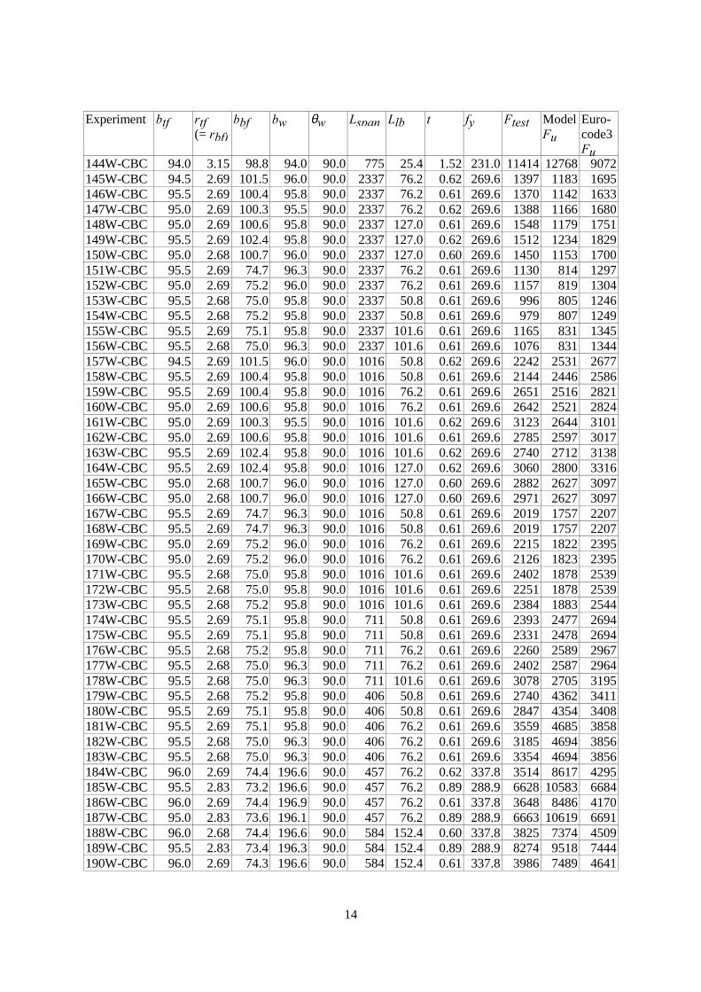
14
Experiment btf rtf(= rbf)
bbf bw θw Lspan Llb t fy Ftest ModelFu
Euro-code3Fu
144W-CBC 94.0 3.15 98.8 94.0 90.0 775 25.4 1.52 231.0 11414 12768 9072145W-CBC 94.5 2.69 101.5 96.0 90.0 2337 76.2 0.62 269.6 1397 1183 1695146W-CBC 95.5 2.69 100.4 95.8 90.0 2337 76.2 0.61 269.6 1370 1142 1633147W-CBC 95.0 2.69 100.3 95.5 90.0 2337 76.2 0.62 269.6 1388 1166 1680148W-CBC 95.0 2.69 100.6 95.8 90.0 2337 127.0 0.61 269.6 1548 1179 1751149W-CBC 95.5 2.69 102.4 95.8 90.0 2337 127.0 0.62 269.6 1512 1234 1829150W-CBC 95.0 2.68 100.7 96.0 90.0 2337 127.0 0.60 269.6 1450 1153 1700151W-CBC 95.5 2.69 74.7 96.3 90.0 2337 76.2 0.61 269.6 1130 814 1297152W-CBC 95.0 2.69 75.2 96.0 90.0 2337 76.2 0.61 269.6 1157 819 1304153W-CBC 95.5 2.68 75.0 95.8 90.0 2337 50.8 0.61 269.6 996 805 1246154W-CBC 95.5 2.68 75.2 95.8 90.0 2337 50.8 0.61 269.6 979 807 1249155W-CBC 95.5 2.69 75.1 95.8 90.0 2337 101.6 0.61 269.6 1165 831 1345156W-CBC 95.5 2.68 75.0 96.3 90.0 2337 101.6 0.61 269.6 1076 831 1344157W-CBC 94.5 2.69 101.5 96.0 90.0 1016 50.8 0.62 269.6 2242 2531 2677158W-CBC 95.5 2.69 100.4 95.8 90.0 1016 50.8 0.61 269.6 2144 2446 2586159W-CBC 95.5 2.69 100.4 95.8 90.0 1016 76.2 0.61 269.6 2651 2516 2821160W-CBC 95.0 2.69 100.6 95.8 90.0 1016 76.2 0.61 269.6 2642 2521 2824161W-CBC 95.0 2.69 100.3 95.5 90.0 1016 101.6 0.62 269.6 3123 2644 3101162W-CBC 95.0 2.69 100.6 95.8 90.0 1016 101.6 0.61 269.6 2785 2597 3017163W-CBC 95.5 2.69 102.4 95.8 90.0 1016 101.6 0.62 269.6 2740 2712 3138164W-CBC 95.5 2.69 102.4 95.8 90.0 1016 127.0 0.62 269.6 3060 2800 3316165W-CBC 95.0 2.68 100.7 96.0 90.0 1016 127.0 0.60 269.6 2882 2627 3097166W-CBC 95.0 2.68 100.7 96.0 90.0 1016 127.0 0.60 269.6 2971 2627 3097167W-CBC 95.5 2.69 74.7 96.3 90.0 1016 50.8 0.61 269.6 2019 1757 2207168W-CBC 95.5 2.69 74.7 96.3 90.0 1016 50.8 0.61 269.6 2019 1757 2207169W-CBC 95.0 2.69 75.2 96.0 90.0 1016 76.2 0.61 269.6 2215 1822 2395170W-CBC 95.0 2.69 75.2 96.0 90.0 1016 76.2 0.61 269.6 2126 1823 2395171W-CBC 95.5 2.68 75.0 95.8 90.0 1016 101.6 0.61 269.6 2402 1878 2539172W-CBC 95.5 2.68 75.0 95.8 90.0 1016 101.6 0.61 269.6 2251 1878 2539173W-CBC 95.5 2.68 75.2 95.8 90.0 1016 101.6 0.61 269.6 2384 1883 2544174W-CBC 95.5 2.69 75.1 95.8 90.0 711 50.8 0.61 269.6 2393 2477 2694175W-CBC 95.5 2.69 75.1 95.8 90.0 711 50.8 0.61 269.6 2331 2478 2694176W-CBC 95.5 2.68 75.2 95.8 90.0 711 76.2 0.61 269.6 2260 2589 2967177W-CBC 95.5 2.68 75.0 96.3 90.0 711 76.2 0.61 269.6 2402 2587 2964178W-CBC 95.5 2.68 75.0 96.3 90.0 711 101.6 0.61 269.6 3078 2705 3195179W-CBC 95.5 2.68 75.2 95.8 90.0 406 50.8 0.61 269.6 2740 4362 3411180W-CBC 95.5 2.69 75.1 95.8 90.0 406 50.8 0.61 269.6 2847 4354 3408181W-CBC 95.5 2.69 75.1 95.8 90.0 406 76.2 0.61 269.6 3559 4685 3858182W-CBC 95.5 2.68 75.0 96.3 90.0 406 76.2 0.61 269.6 3185 4694 3856183W-CBC 95.5 2.68 75.0 96.3 90.0 406 76.2 0.61 269.6 3354 4694 3856184W-CBC 96.0 2.69 74.4 196.6 90.0 457 76.2 0.62 337.8 3514 8617 4295185W-CBC 95.5 2.83 73.2 196.6 90.0 457 76.2 0.89 288.9 6628 10583 6684186W-CBC 96.0 2.69 74.4 196.9 90.0 457 76.2 0.61 337.8 3648 8486 4170187W-CBC 95.0 2.83 73.6 196.1 90.0 457 76.2 0.89 288.9 6663 10619 6691188W-CBC 96.0 2.68 74.4 196.6 90.0 584 152.4 0.60 337.8 3825 7374 4509189W-CBC 95.5 2.83 73.4 196.3 90.0 584 152.4 0.89 288.9 8274 9518 7444190W-CBC 96.0 2.69 74.3 196.6 90.0 584 152.4 0.61 337.8 3986 7489 4641
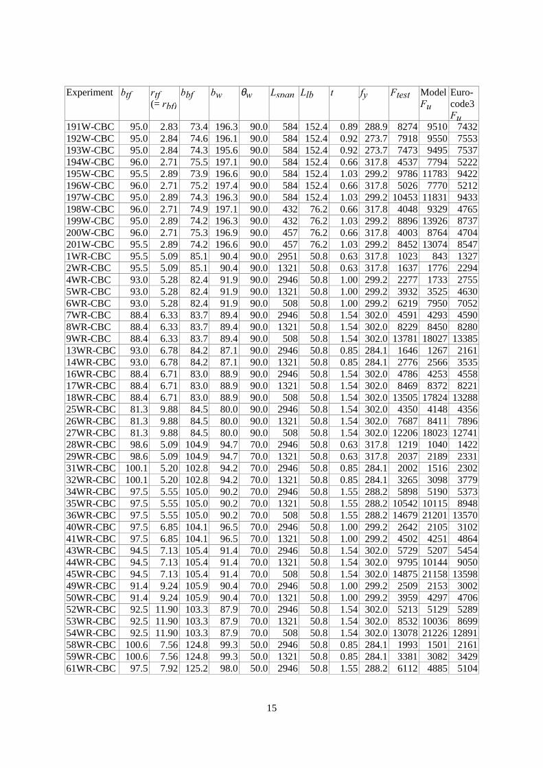
15
Experiment btf rtf(= rbf)
bbf bw θw Lspan Llb t fy Ftest ModelFu
Euro-code3Fu
191W-CBC 95.0 2.83 73.4 196.3 90.0 584 152.4 0.89 288.9 8274 9510 7432192W-CBC 95.0 2.84 74.6 196.1 90.0 584 152.4 0.92 273.7 7918 9550 7553193W-CBC 95.0 2.84 74.3 195.6 90.0 584 152.4 0.92 273.7 7473 9495 7537194W-CBC 96.0 2.71 75.5 197.1 90.0 584 152.4 0.66 317.8 4537 7794 5222195W-CBC 95.5 2.89 73.9 196.6 90.0 584 152.4 1.03 299.2 9786 11783 9422196W-CBC 96.0 2.71 75.2 197.4 90.0 584 152.4 0.66 317.8 5026 7770 5212197W-CBC 95.0 2.89 74.3 196.3 90.0 584 152.4 1.03 299.2 10453 11831 9433198W-CBC 96.0 2.71 74.9 197.1 90.0 432 76.2 0.66 317.8 4048 9329 4765199W-CBC 95.0 2.89 74.2 196.3 90.0 432 76.2 1.03 299.2 8896 13926 8737200W-CBC 96.0 2.71 75.3 196.9 90.0 457 76.2 0.66 317.8 4003 8764 4704201W-CBC 95.5 2.89 74.2 196.6 90.0 457 76.2 1.03 299.2 8452 13074 85471WR-CBC 95.5 5.09 85.1 90.4 90.0 2951 50.8 0.63 317.8 1023 843 13272WR-CBC 95.5 5.09 85.1 90.4 90.0 1321 50.8 0.63 317.8 1637 1776 22944WR-CBC 93.0 5.28 82.4 91.9 90.0 2946 50.8 1.00 299.2 2277 1733 27555WR-CBC 93.0 5.28 82.4 91.9 90.0 1321 50.8 1.00 299.2 3932 3525 46306WR-CBC 93.0 5.28 82.4 91.9 90.0 508 50.8 1.00 299.2 6219 7950 70527WR-CBC 88.4 6.33 83.7 89.4 90.0 2946 50.8 1.54 302.0 4591 4293 45908WR-CBC 88.4 6.33 83.7 89.4 90.0 1321 50.8 1.54 302.0 8229 8450 82809WR-CBC 88.4 6.33 83.7 89.4 90.0 508 50.8 1.54 302.0 13781 18027 1338513WR-CBC 93.0 6.78 84.2 87.1 90.0 2946 50.8 0.85 284.1 1646 1267 216114WR-CBC 93.0 6.78 84.2 87.1 90.0 1321 50.8 0.85 284.1 2776 2566 353516WR-CBC 88.4 6.71 83.0 88.9 90.0 2946 50.8 1.54 302.0 4786 4253 455817WR-CBC 88.4 6.71 83.0 88.9 90.0 1321 50.8 1.54 302.0 8469 8372 822118WR-CBC 88.4 6.71 83.0 88.9 90.0 508 50.8 1.54 302.0 13505 17824 1328825WR-CBC 81.3 9.88 84.5 80.0 90.0 2946 50.8 1.54 302.0 4350 4148 435626WR-CBC 81.3 9.88 84.5 80.0 90.0 1321 50.8 1.54 302.0 7687 8411 789627WR-CBC 81.3 9.88 84.5 80.0 90.0 508 50.8 1.54 302.0 12206 18023 1274128WR-CBC 98.6 5.09 104.9 94.7 70.0 2946 50.8 0.63 317.8 1219 1040 142229WR-CBC 98.6 5.09 104.9 94.7 70.0 1321 50.8 0.63 317.8 2037 2189 233131WR-CBC 100.1 5.20 102.8 94.2 70.0 2946 50.8 0.85 284.1 2002 1516 230232WR-CBC 100.1 5.20 102.8 94.2 70.0 1321 50.8 0.85 284.1 3265 3098 377934WR-CBC 97.5 5.55 105.0 90.2 70.0 2946 50.8 1.55 288.2 5898 5190 537335WR-CBC 97.5 5.55 105.0 90.2 70.0 1321 50.8 1.55 288.2 10542 10115 894836WR-CBC 97.5 5.55 105.0 90.2 70.0 508 50.8 1.55 288.2 14679 21201 1357040WR-CBC 97.5 6.85 104.1 96.5 70.0 2946 50.8 1.00 299.2 2642 2105 310241WR-CBC 97.5 6.85 104.1 96.5 70.0 1321 50.8 1.00 299.2 4502 4251 486443WR-CBC 94.5 7.13 105.4 91.4 70.0 2946 50.8 1.54 302.0 5729 5207 545444WR-CBC 94.5 7.13 105.4 91.4 70.0 1321 50.8 1.54 302.0 9795 10144 905045WR-CBC 94.5 7.13 105.4 91.4 70.0 508 50.8 1.54 302.0 14875 21158 1359849WR-CBC 91.4 9.24 105.9 90.4 70.0 2946 50.8 1.00 299.2 2509 2153 300250WR-CBC 91.4 9.24 105.9 90.4 70.0 1321 50.8 1.00 299.2 3959 4297 470652WR-CBC 92.5 11.90 103.3 87.9 70.0 2946 50.8 1.54 302.0 5213 5129 528953WR-CBC 92.5 11.90 103.3 87.9 70.0 1321 50.8 1.54 302.0 8532 10036 869954WR-CBC 92.5 11.90 103.3 87.9 70.0 508 50.8 1.54 302.0 13078 21226 1289158WR-CBC 100.6 7.56 124.8 99.3 50.0 2946 50.8 0.85 284.1 1993 1501 216159WR-CBC 100.6 7.56 124.8 99.3 50.0 1321 50.8 0.85 284.1 3381 3082 342961WR-CBC 97.5 7.92 125.2 98.0 50.0 2946 50.8 1.55 288.2 6112 4885 5104
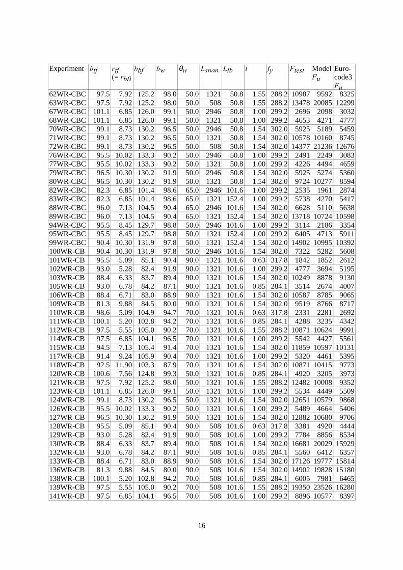
16
Experiment btf rtf(= rbf)
bbf bw θw Lspan Llb t fy Ftest ModelFu
Euro-code3Fu
62WR-CBC 97.5 7.92 125.2 98.0 50.0 1321 50.8 1.55 288.2 10987 9592 832563WR-CBC 97.5 7.92 125.2 98.0 50.0 508 50.8 1.55 288.2 13478 20085 1229967WR-CBC 101.1 6.85 126.0 99.1 50.0 2946 50.8 1.00 299.2 2696 2098 303268WR-CBC 101.1 6.85 126.0 99.1 50.0 1321 50.8 1.00 299.2 4653 4271 477770WR-CBC 99.1 8.73 130.2 96.5 50.0 2946 50.8 1.54 302.0 5925 5189 545971WR-CBC 99.1 8.73 130.2 96.5 50.0 1321 50.8 1.54 302.0 10578 10160 874572WR-CBC 99.1 8.73 130.2 96.5 50.0 508 50.8 1.54 302.0 14377 21236 1267676WR-CBC 95.5 10.02 133.3 90.2 50.0 2946 50.8 1.00 299.2 2491 2249 308377WR-CBC 95.5 10.02 133.3 90.2 50.0 1321 50.8 1.00 299.2 4226 4494 465979WR-CBC 96.5 10.30 130.2 91.9 50.0 2946 50.8 1.54 302.0 5925 5274 536080WR-CBC 96.5 10.30 130.2 91.9 50.0 1321 50.8 1.54 302.0 9724 10277 859482WR-CBC 82.3 6.85 101.4 98.6 65.0 2946 101.6 1.00 299.2 2535 1961 287483WR-CBC 82.3 6.85 101.4 98.6 65.0 1321 152.4 1.00 299.2 5738 4270 541788WR-CBC 96.0 7.13 104.5 90.4 65.0 2946 101.6 1.54 302.0 6628 5110 563889WR-CBC 96.0 7.13 104.5 90.4 65.0 1321 152.4 1.54 302.0 13718 10724 1059894WR-CBC 95.5 8.45 129.7 98.8 50.0 2946 101.6 1.00 299.2 3114 2186 335495WR-CBC 95.5 8.45 129.7 98.8 50.0 1321 152.4 1.00 299.2 6405 4713 591199WR-CBC 90.4 10.30 131.9 97.8 50.0 1321 152.4 1.54 302.0 14902 10995 10392100WR-CB 90.4 10.30 131.9 97.8 50.0 2946 101.6 1.54 302.0 7322 5282 5608101WR-CB 95.5 5.09 85.1 90.4 90.0 1321 101.6 0.63 317.8 1842 1852 2612102WR-CB 93.0 5.28 82.4 91.9 90.0 1321 101.6 1.00 299.2 4777 3694 5195103WR-CB 88.4 6.33 83.7 89.4 90.0 1321 101.6 1.54 302.0 10249 8878 9130105WR-CB 93.0 6.78 84.2 87.1 90.0 1321 101.6 0.85 284.1 3514 2674 4007106WR-CB 88.4 6.71 83.0 88.9 90.0 1321 101.6 1.54 302.0 10587 8785 9065109WR-CB 81.3 9.88 84.5 80.0 90.0 1321 101.6 1.54 302.0 9519 8766 8717110WR-CB 98.6 5.09 104.9 94.7 70.0 1321 101.6 0.63 317.8 2331 2281 2692111WR-CB 100.1 5.20 102.8 94.2 70.0 1321 101.6 0.85 284.1 4288 3235 4342112WR-CB 97.5 5.55 105.0 90.2 70.0 1321 101.6 1.55 288.2 10871 10624 9991114WR-CB 97.5 6.85 104.1 96.5 70.0 1321 101.6 1.00 299.2 5542 4427 5561115WR-CB 94.5 7.13 105.4 91.4 70.0 1321 101.6 1.54 302.0 11859 10597 10131117WR-CB 91.4 9.24 105.9 90.4 70.0 1321 101.6 1.00 299.2 5320 4461 5395118WR-CB 92.5 11.90 103.3 87.9 70.0 1321 101.6 1.54 302.0 10871 10415 9773120WR-CB 100.6 7.56 124.8 99.3 50.0 1321 101.6 0.85 284.1 4920 3205 3973121WR-CB 97.5 7.92 125.2 98.0 50.0 1321 101.6 1.55 288.2 12482 10008 9352123WR-CB 101.1 6.85 126.0 99.1 50.0 1321 101.6 1.00 299.2 5534 4449 5509124WR-CB 99.1 8.73 130.2 96.5 50.0 1321 101.6 1.54 302.0 12651 10579 9868126WR-CB 95.5 10.02 133.3 90.2 50.0 1321 101.6 1.00 299.2 5489 4664 5406127WR-CB 96.5 10.30 130.2 91.9 50.0 1321 101.6 1.54 302.0 12882 10680 9706128WR-CB 95.5 5.09 85.1 90.4 90.0 508 101.6 0.63 317.8 3381 4920 4444129WR-CB 93.0 5.28 82.4 91.9 90.0 508 101.6 1.00 299.2 7784 8856 8534130WR-CB 88.4 6.33 83.7 89.4 90.0 508 101.6 1.54 302.0 16681 20029 15929132WR-CB 93.0 6.78 84.2 87.1 90.0 508 101.6 0.85 284.1 5560 6412 6357133WR-CB 88.4 6.71 83.0 88.9 90.0 508 101.6 1.54 302.0 17126 19777 15814136WR-CB 81.3 9.88 84.5 80.0 90.0 508 101.6 1.54 302.0 14902 19828 15180138WR-CB 100.1 5.20 102.8 94.2 70.0 508 101.6 0.85 284.1 6005 7981 6465139WR-CB 97.5 5.55 105.0 90.2 70.0 508 101.6 1.55 288.2 19350 23526 16280141WR-CB 97.5 6.85 104.1 96.5 70.0 508 101.6 1.00 299.2 8896 10577 8397
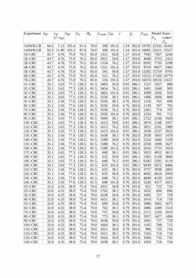
17
Experiment btf rtf(= rbf)
bbf bw θw Lspan Llb t fy Ftest ModelFu
Euro-code3Fu
142WR-CB 94.5 7.13 105.4 91.4 70.0 508 101.6 1.54 302.0 19795 23333 16342145WR-CB 92.5 11.90 103.3 87.9 70.0 508 101.6 1.54 302.0 16681 23221 155271E-CBC 43.7 4.76 75.9 76.5 85.0 1321 50.8 1.57 293.0 7945 7567 52442E-CBC 43.7 4.76 75.9 76.5 85.0 2921 50.8 1.57 293.0 4048 3755 23223E-CBC 43.7 4.76 75.9 76.5 85.0 1334 76.2 1.57 293.0 8505 7720 52984E-CBC 43.7 4.76 75.9 76.5 85.0 1321 101.6 1.57 293.0 9519 8027 54655E-CBC 43.7 4.76 75.9 76.5 85.0 541 50.8 1.57 293.0 13282 15759 97056E-CBC 43.7 4.76 75.9 76.5 85.0 521 76.2 1.57 293.0 15515 17220 107707E-CBC 43.7 4.76 75.9 76.5 85.0 516 101.6 1.57 293.0 16974 18516 116571C-CBC 35.1 3.63 77.3 128.3 81.5 3493 50.8 0.91 286.1 1557 1027 8882C-CBC 35.1 3.63 77.3 128.3 81.5 3454 76.2 0.91 286.1 1601 1048 9053C-CBC 35.1 3.63 77.3 128.3 81.5 3462 101.6 0.91 286.1 1699 1056 9104C-CBC 35.1 3.63 77.3 128.3 81.5 3556 38.1 0.91 286.1 1406 1004 8695C-CBC 35.1 3.56 77.6 128.5 81.5 3556 38.1 0.76 282.0 1210 763 6996C-CBC 35.1 3.56 77.6 128.5 81.5 3556 50.8 0.76 282.0 1139 767 7027C-CBC 35.1 3.56 77.6 128.5 81.5 3556 76.2 0.76 282.0 1281 774 7078C-CBC 35.1 3.56 77.6 128.5 81.5 3556 101.6 0.76 282.0 1254 781 7129C-CBC 35.1 3.63 77.3 128.3 81.5 1600 38.1 0.91 286.1 2722 2144 192010C-CBC 35.1 3.63 77.3 128.3 81.5 1613 50.8 0.91 286.1 2874 2148 195711C-CBC 35.1 3.63 77.3 128.3 81.5 1613 76.2 0.91 286.1 3051 2191 198912C-CBC 35.1 3.63 77.3 128.3 81.5 1613 101.6 0.91 286.1 3336 2237 202313C-CBC 35.1 3.56 77.6 128.5 81.5 1638 38.1 0.76 282.0 2028 1603 147814C-CBC 35.1 3.56 77.6 128.5 81.5 1588 50.8 0.76 282.0 2224 1666 155915C-CBC 35.1 3.56 77.6 128.5 81.5 1588 76.2 0.76 282.0 2358 1698 162716C-CBC 35.1 3.56 77.6 128.5 81.5 1588 101.6 0.76 282.0 2616 1733 165417C-CBC 35.1 3.63 77.3 128.3 81.5 648 38.1 0.91 286.1 5053 4952 361318C-CBC 35.1 3.63 77.3 128.3 81.5 635 50.8 0.91 286.1 5365 5158 384619C-CBC 35.1 3.63 77.3 128.3 81.5 648 76.2 0.91 286.1 6183 5292 411920C-CBC 35.1 3.63 77.3 128.3 81.5 635 101.6 0.91 286.1 6939 5672 446621C-CBC 35.1 3.56 77.6 128.5 81.5 635 38.1 0.76 282.0 3737 3938 280322C-CBC 35.1 3.56 77.6 128.5 81.5 635 50.8 0.76 282.0 4092 4024 295923C-CBC 35.1 3.56 77.6 128.5 81.5 648 76.2 0.76 282.0 4849 4120 318324C-CBC 35.1 3.56 77.6 128.5 81.5 648 101.6 0.76 282.0 5320 4317 34121U-CBC 32.0 4.35 38.9 75.4 70.0 1651 50.8 0.79 291.6 952 722 7242U-CBC 32.0 4.35 38.9 75.4 70.0 1702 38.1 0.79 291.6 1032 694 6963U-CBC 32.0 4.35 38.9 75.4 70.0 1638 50.8 0.79 291.6 1085 727 7294U-CBC 32.0 4.35 38.9 75.4 70.0 1651 38.1 0.79 291.6 1014 714 7185U-CBC 32.0 4.35 38.9 75.4 70.0 699 50.8 0.79 291.6 1886 1602 16756U-CBC 32.0 4.35 38.9 75.4 70.0 762 38.1 0.79 291.6 1886 1449 15147U-CBC 32.0 4.35 38.9 75.4 70.0 737 50.8 0.79 291.6 2171 1526 16108U-CBC 32.0 4.35 38.9 75.4 70.0 775 38.1 0.79 291.6 1957 1427 14969U-CBC 32.0 4.35 38.9 75.4 70.0 1638 50.8 0.79 291.6 1041 727 72910U-CBC 32.0 4.35 38.9 75.4 70.0 1664 38.1 0.79 291.6 1165 708 71211U-CBC 32.0 4.35 38.9 75.4 70.0 1651 50.8 0.79 291.6 996 722 72412U-CBC 32.0 4.35 38.9 75.4 70.0 1651 38.1 0.79 291.6 1165 714 71813U-CBC 32.0 4.35 38.9 75.4 70.0 1626 50.8 0.79 291.6 1094 732 73514U-CBC 32.0 4.35 38.9 75.4 70.0 1638 38.1 0.79 291.6 1050 719 724
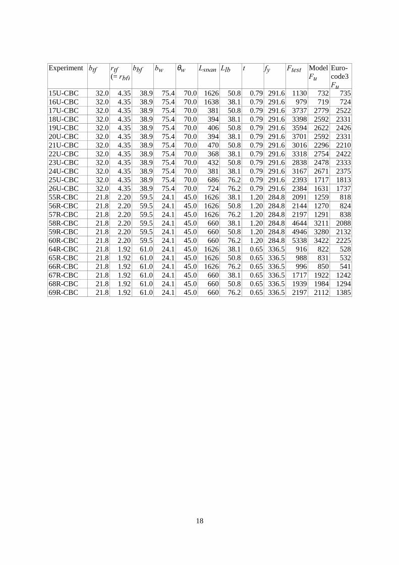
18
Experiment btf rtf(= rbf)
bbf bw θw Lspan Llb t fy Ftest ModelFu
Euro-code3Fu
15U-CBC 32.0 4.35 38.9 75.4 70.0 1626 50.8 0.79 291.6 1130 732 73516U-CBC 32.0 4.35 38.9 75.4 70.0 1638 38.1 0.79 291.6 979 719 72417U-CBC 32.0 4.35 38.9 75.4 70.0 381 50.8 0.79 291.6 3737 2779 252218U-CBC 32.0 4.35 38.9 75.4 70.0 394 38.1 0.79 291.6 3398 2592 233119U-CBC 32.0 4.35 38.9 75.4 70.0 406 50.8 0.79 291.6 3594 2622 242620U-CBC 32.0 4.35 38.9 75.4 70.0 394 38.1 0.79 291.6 3701 2592 233121U-CBC 32.0 4.35 38.9 75.4 70.0 470 50.8 0.79 291.6 3016 2296 221022U-CBC 32.0 4.35 38.9 75.4 70.0 368 38.1 0.79 291.6 3318 2754 242223U-CBC 32.0 4.35 38.9 75.4 70.0 432 50.8 0.79 291.6 2838 2478 233324U-CBC 32.0 4.35 38.9 75.4 70.0 381 38.1 0.79 291.6 3167 2671 237525U-CBC 32.0 4.35 38.9 75.4 70.0 686 76.2 0.79 291.6 2393 1717 181326U-CBC 32.0 4.35 38.9 75.4 70.0 724 76.2 0.79 291.6 2384 1631 173755R-CBC 21.8 2.20 59.5 24.1 45.0 1626 38.1 1.20 284.8 2091 1259 81856R-CBC 21.8 2.20 59.5 24.1 45.0 1626 50.8 1.20 284.8 2144 1270 82457R-CBC 21.8 2.20 59.5 24.1 45.0 1626 76.2 1.20 284.8 2197 1291 83858R-CBC 21.8 2.20 59.5 24.1 45.0 660 38.1 1.20 284.8 4644 3211 208859R-CBC 21.8 2.20 59.5 24.1 45.0 660 50.8 1.20 284.8 4946 3280 213260R-CBC 21.8 2.20 59.5 24.1 45.0 660 76.2 1.20 284.8 5338 3422 222564R-CBC 21.8 1.92 61.0 24.1 45.0 1626 38.1 0.65 336.5 916 822 52865R-CBC 21.8 1.92 61.0 24.1 45.0 1626 50.8 0.65 336.5 988 831 53266R-CBC 21.8 1.92 61.0 24.1 45.0 1626 76.2 0.65 336.5 996 850 54167R-CBC 21.8 1.92 61.0 24.1 45.0 660 38.1 0.65 336.5 1717 1922 124268R-CBC 21.8 1.92 61.0 24.1 45.0 660 50.8 0.65 336.5 1939 1984 129469R-CBC 21.8 1.92 61.0 24.1 45.0 660 76.2 0.65 336.5 2197 2112 1385
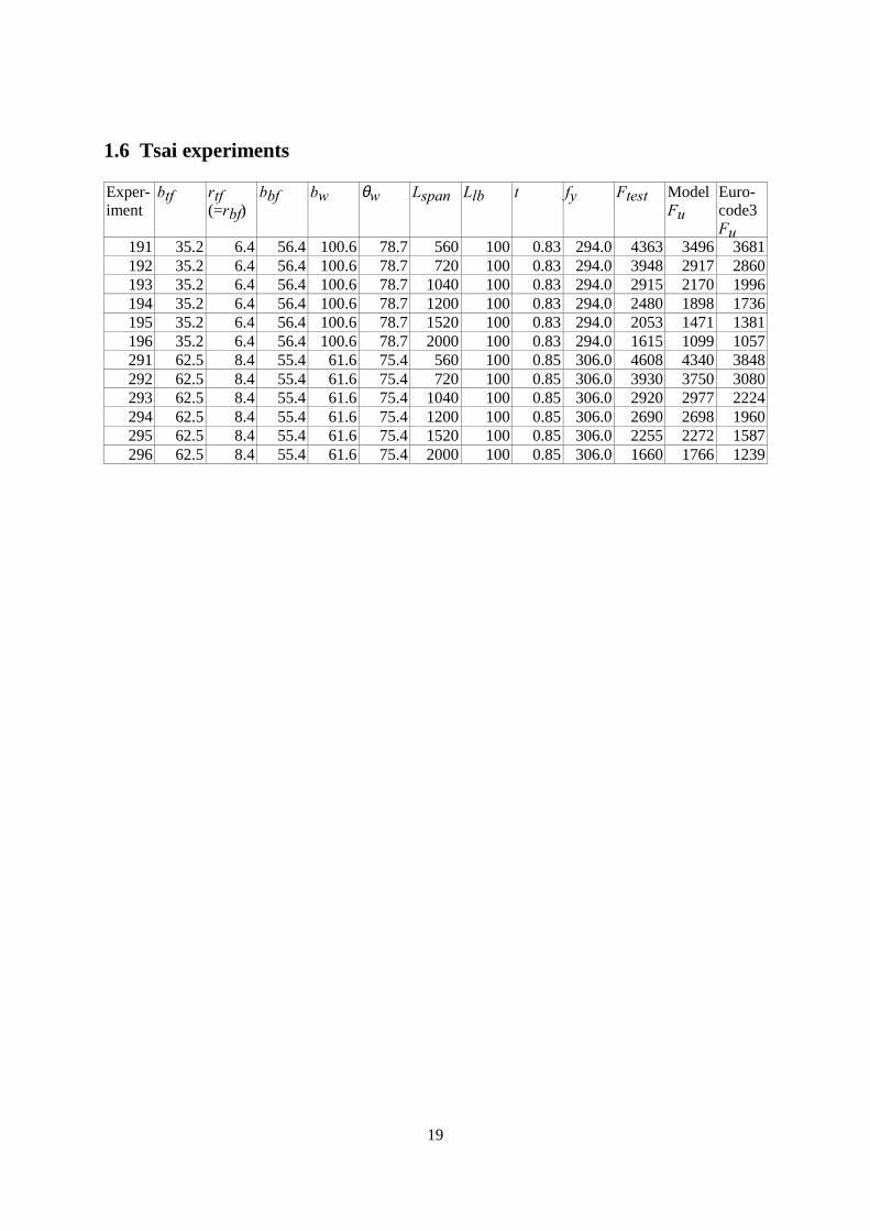
19
1.6 Tsai experiments
Exper-iment
btf rtf(=rbf)
bbf bw θw Lspan Llb t fy Ftest ModelFu
Euro-code3Fu
191 35.2 6.4 56.4 100.6 78.7 560 100 0.83 294.0 4363 3496 3681192 35.2 6.4 56.4 100.6 78.7 720 100 0.83 294.0 3948 2917 2860193 35.2 6.4 56.4 100.6 78.7 1040 100 0.83 294.0 2915 2170 1996194 35.2 6.4 56.4 100.6 78.7 1200 100 0.83 294.0 2480 1898 1736195 35.2 6.4 56.4 100.6 78.7 1520 100 0.83 294.0 2053 1471 1381196 35.2 6.4 56.4 100.6 78.7 2000 100 0.83 294.0 1615 1099 1057291 62.5 8.4 55.4 61.6 75.4 560 100 0.85 306.0 4608 4340 3848292 62.5 8.4 55.4 61.6 75.4 720 100 0.85 306.0 3930 3750 3080293 62.5 8.4 55.4 61.6 75.4 1040 100 0.85 306.0 2920 2977 2224294 62.5 8.4 55.4 61.6 75.4 1200 100 0.85 306.0 2690 2698 1960295 62.5 8.4 55.4 61.6 75.4 1520 100 0.85 306.0 2255 2272 1587296 62.5 8.4 55.4 61.6 75.4 2000 100 0.85 306.0 1660 1766 1239
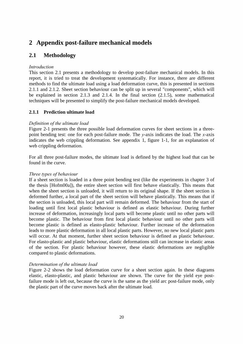
20
2 Appendix post-failure mechanical models
2.1 Methodology
IntroductionThis section 2.1 presents a methodology to develop post-failure mechanical models. In thisreport, it is tried to treat the development systematically. For instance, there are differentmethods to find the ultimate load using a load deformation curve, this is presented in sections2.1.1 and 2.1.2. Sheet section behaviour can be split up in several "components", which willbe explained in section 2.1.3 and 2.1.4. In the final section (2.1.5), some mathematicaltechniques will be presented to simplify the post-failure mechanical models developed.
2.1.1 Prediction ultimate load
Definition of the ultimate loadFigure 2-1 presents the three possible load deformation curves for sheet sections in a three-point bending test: one for each post-failure mode. The y-axis indicates the load. The x-axisindicates the web crippling deformation. See appendix 1, figure 1-1, for an explanation ofweb crippling deformation.
For all three post-failure modes, the ultimate load is defined by the highest load that can befound in the curve.
Three types of behaviourIf a sheet section is loaded in a three point bending test (like the experiments in chapter 3 ofthe thesis [Hofm00a]), the entire sheet section will first behave elastically. This means thatwhen the sheet section is unloaded, it will return to its original shape. If the sheet section isdeformed further, a local part of the sheet section will behave plastically. This means that ifthe section is unloaded, this local part will remain deformed. The behaviour from the start ofloading until first local plastic behaviour is defined as elastic behaviour. During furtherincrease of deformation, increasingly local parts will become plastic until no other parts willbecome plastic. The behaviour from first local plastic behaviour until no other parts willbecome plastic is defined as elasto-plastic behaviour. Further increase of the deformationleads to more plastic deformation in all local plastic parts. However, no new local plastic partswill occur. At that moment, further sheet section behaviour is defined as plastic behaviour.For elasto-plastic and plastic behaviour, elastic deformations still can increase in elastic areasof the section. For plastic behaviour however, these elastic deformations are negligiblecompared to plastic deformations.
Determination of the ultimate loadFigure 2-2 shows the load deformation curve for a sheet section again. In these diagramselastic, elasto-plastic, and plastic behaviour are shown. The curve for the yield eye post-failure mode is left out, because the curve is the same as the yield arc post-failure mode, onlythe plastic part of the curve moves back after the ultimate load.
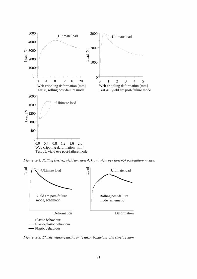
21
0 4 8 12 16 20Web crippling deformation [mm]Test 8, rolling post-failure mode
0
1000
2000
3000
4000
5000
Load
[N]
0 1 2 3 4 5Web crippling deformation [mm]Test 41, yield arc post-failure mode
0
1000
2000
3000
0.0 0.4 0.8 1.2 1.6 2.0Web crippling deformation [mm]Test 65, yield eye post-failure mode
0
400
800
1200
1600
2000
Load
[N]
Load
[N]
Ultimate load
Ultimate load
Ultimate load
Figure 2-1. Rolling (test 8), yield arc (test 41), and yield eye (test 65) post-failure modes.
Deformation
Load Ultimate load Ultimate load
Elastic behaviourElasto-plastic behaviourPlastic behaviour
Load
Deformation
Yield arc post-failuremode, schematic
Rolling post-failuremode, schematic
Figure 2-2. Elastic, elasto-plastic, and plastic behaviour of a sheet section.
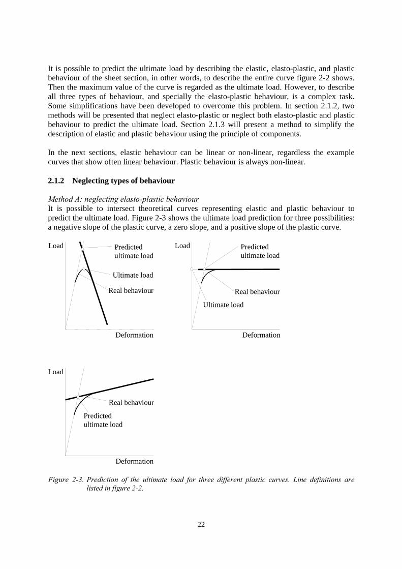
22
It is possible to predict the ultimate load by describing the elastic, elasto-plastic, and plasticbehaviour of the sheet section, in other words, to describe the entire curve figure 2-2 shows.Then the maximum value of the curve is regarded as the ultimate load. However, to describeall three types of behaviour, and specially the elasto-plastic behaviour, is a complex task.Some simplifications have been developed to overcome this problem. In section 2.1.2, twomethods will be presented that neglect elasto-plastic or neglect both elasto-plastic and plasticbehaviour to predict the ultimate load. Section 2.1.3 will present a method to simplify thedescription of elastic and plastic behaviour using the principle of components.
In the next sections, elastic behaviour can be linear or non-linear, regardless the examplecurves that show often linear behaviour. Plastic behaviour is always non-linear.
2.1.2 Neglecting types of behaviour
Method A: neglecting elasto-plastic behaviourIt is possible to intersect theoretical curves representing elastic and plastic behaviour topredict the ultimate load. Figure 2-3 shows the ultimate load prediction for three possibilities:a negative slope of the plastic curve, a zero slope, and a positive slope of the plastic curve.
Predictedultimate load
Real behaviour
Ultimate load
Predictedultimate load
Real behaviour
Ultimate load
Predictedultimate load
Real behaviour
Load Load
Load
Deformation Deformation
Deformation
Figure 2-3. Prediction of the ultimate load for three different plastic curves. Line definitions arelisted in figure 2-2.
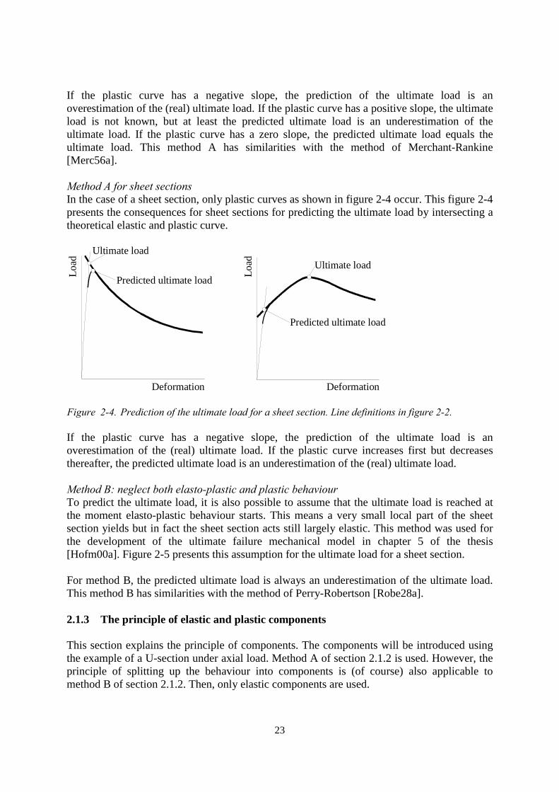
23
If the plastic curve has a negative slope, the prediction of the ultimate load is anoverestimation of the (real) ultimate load. If the plastic curve has a positive slope, the ultimateload is not known, but at least the predicted ultimate load is an underestimation of theultimate load. If the plastic curve has a zero slope, the predicted ultimate load equals theultimate load. This method A has similarities with the method of Merchant-Rankine[Merc56a].
Method A for sheet sectionsIn the case of a sheet section, only plastic curves as shown in figure 2-4 occur. This figure 2-4presents the consequences for sheet sections for predicting the ultimate load by intersecting atheoretical elastic and plastic curve.
Deformation
Load
Ultimate loadUltimate load
Load
Deformation
Predicted ultimate load
Predicted ultimate load
Figure 2-4. Prediction of the ultimate load for a sheet section. Line definitions in figure 2-2.
If the plastic curve has a negative slope, the prediction of the ultimate load is anoverestimation of the (real) ultimate load. If the plastic curve increases first but decreasesthereafter, the predicted ultimate load is an underestimation of the (real) ultimate load.
Method B: neglect both elasto-plastic and plastic behaviourTo predict the ultimate load, it is also possible to assume that the ultimate load is reached atthe moment elasto-plastic behaviour starts. This means a very small local part of the sheetsection yields but in fact the sheet section acts still largely elastic. This method was used forthe development of the ultimate failure mechanical model in chapter 5 of the thesis[Hofm00a]. Figure 2-5 presents this assumption for the ultimate load for a sheet section.
For method B, the predicted ultimate load is always an underestimation of the ultimate load.This method B has similarities with the method of Perry-Robertson [Robe28a].
2.1.3 The principle of elastic and plastic components
This section explains the principle of components. The components will be introduced usingthe example of a U-section under axial load. Method A of section 2.1.2 is used. However, theprinciple of splitting up the behaviour into components is (of course) also applicable tomethod B of section 2.1.2. Then, only elastic components are used.
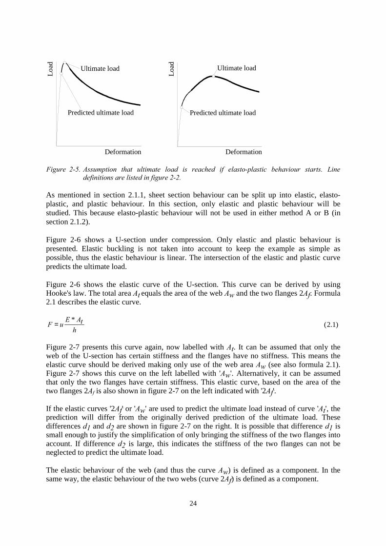
24
Deformation
Load Ultimate load Ultimate load
Load
Deformation
Predicted ultimate load Predicted ultimate load
Figure 2-5. Assumption that ultimate load is reached if elasto-plastic behaviour starts. Linedefinitions are listed in figure 2-2.
As mentioned in section 2.1.1, sheet section behaviour can be split up into elastic, elasto-plastic, and plastic behaviour. In this section, only elastic and plastic behaviour will bestudied. This because elasto-plastic behaviour will not be used in either method A or B (insection 2.1.2).
Figure 2-6 shows a U-section under compression. Only elastic and plastic behaviour ispresented. Elastic buckling is not taken into account to keep the example as simple aspossible, thus the elastic behaviour is linear. The intersection of the elastic and plastic curvepredicts the ultimate load.
Figure 2-6 shows the elastic curve of the U-section. This curve can be derived by usingHooke's law. The total area At equals the area of the web Aw and the two flanges 2Af. Formula2.1 describes the elastic curve.
htAE
uF*
= (2.1)
Figure 2-7 presents this curve again, now labelled with At. It can be assumed that only theweb of the U-section has certain stiffness and the flanges have no stiffness. This means theelastic curve should be derived making only use of the web area Aw (see also formula 2.1).Figure 2-7 shows this curve on the left labelled with 'Aw'. Alternatively, it can be assumedthat only the two flanges have certain stiffness. This elastic curve, based on the area of thetwo flanges 2Af is also shown in figure 2-7 on the left indicated with '2Af'.
If the elastic curves '2Af' or 'Aw' are used to predict the ultimate load instead of curve 'At', theprediction will differ from the originally derived prediction of the ultimate load. Thesedifferences d1 and d2 are shown in figure 2-7 on the right. It is possible that difference d1 issmall enough to justify the simplification of only bringing the stiffness of the two flanges intoaccount. If difference d2 is large, this indicates the stiffness of the two flanges can not beneglected to predict the ultimate load.
The elastic behaviour of the web (and thus the curve Aw) is defined as a component. In thesame way, the elastic behaviour of the two webs (curve 2Af) is defined as a component.

25
u F
Elastic behaviour Plastic behaviour
Fu
Yield lines
u
FPredictedultimate load
h
Web (area Aw) Flanges (area 2Af)
Figure 2-6. U-section under compression. Intersection of elastic and plastic curves predicts theultimate load.
u
F At Aw2Af
u
F At Aw2AfPredictedultimate load
Alternative predictedultimate load usingcurve
Alternative predictedultimate load usingcurve
d1
d2
Aw
2Af
Figure 2-7. On the left different elastic curves for the U-section. On the right predictions of theultimate load are made for different elastic curves.
Plastic components U-sectionPlastic behaviour can be split up into components using the same method as for elasticcomponents. Figure 2-6 on the right shows the U-section plastically deformed. Yield lines arelocated in the web and in the two flanges. Now, it is assumed that only in the web yield lines
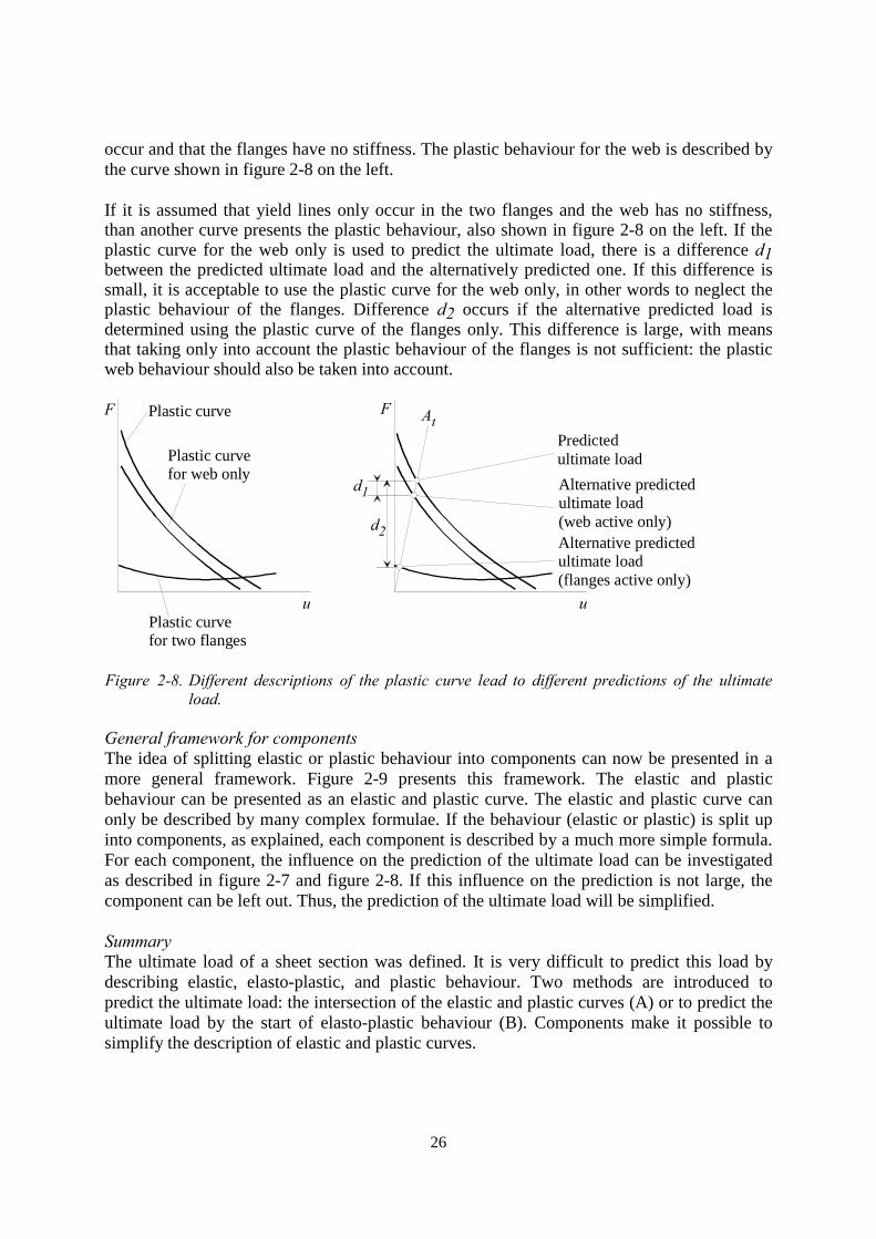
26
occur and that the flanges have no stiffness. The plastic behaviour for the web is described bythe curve shown in figure 2-8 on the left.
If it is assumed that yield lines only occur in the two flanges and the web has no stiffness,than another curve presents the plastic behaviour, also shown in figure 2-8 on the left. If theplastic curve for the web only is used to predict the ultimate load, there is a difference d1between the predicted ultimate load and the alternatively predicted one. If this difference issmall, it is acceptable to use the plastic curve for the web only, in other words to neglect theplastic behaviour of the flanges. Difference d2 occurs if the alternative predicted load isdetermined using the plastic curve of the flanges only. This difference is large, with meansthat taking only into account the plastic behaviour of the flanges is not sufficient: the plasticweb behaviour should also be taken into account.
u
F
u
F AtPredictedultimate load
Alternative predictedultimate load(flanges active only)
Alternative predictedultimate load(web active only)
d1
d2
Plastic curve
Plastic curvefor web only
Plastic curvefor two flanges
Figure 2-8. Different descriptions of the plastic curve lead to different predictions of the ultimateload.
General framework for componentsThe idea of splitting elastic or plastic behaviour into components can now be presented in amore general framework. Figure 2-9 presents this framework. The elastic and plasticbehaviour can be presented as an elastic and plastic curve. The elastic and plastic curve canonly be described by many complex formulae. If the behaviour (elastic or plastic) is split upinto components, as explained, each component is described by a much more simple formula.For each component, the influence on the prediction of the ultimate load can be investigatedas described in figure 2-7 and figure 2-8. If this influence on the prediction is not large, thecomponent can be left out. Thus, the prediction of the ultimate load will be simplified.
SummaryThe ultimate load of a sheet section was defined. It is very difficult to predict this load bydescribing elastic, elasto-plastic, and plastic behaviour. Two methods are introduced topredict the ultimate load: the intersection of the elastic and plastic curves (A) or to predict theultimate load by the start of elasto-plastic behaviour (B). Components make it possible tosimplify the description of elastic and plastic curves.
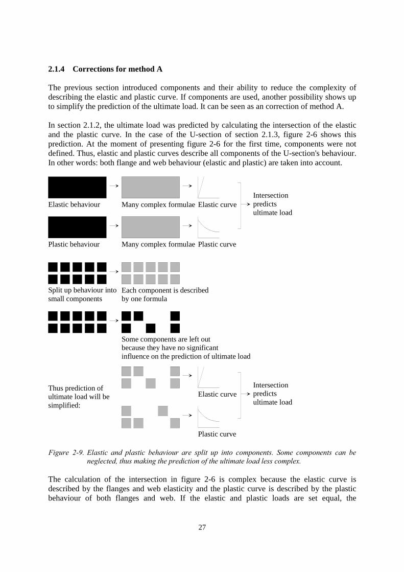
27
2.1.4 Corrections for method A
The previous section introduced components and their ability to reduce the complexity ofdescribing the elastic and plastic curve. If components are used, another possibility shows upto simplify the prediction of the ultimate load. It can be seen as an correction of method A.
In section 2.1.2, the ultimate load was predicted by calculating the intersection of the elasticand the plastic curve. In the case of the U-section of section 2.1.3, figure 2-6 shows thisprediction. At the moment of presenting figure 2-6 for the first time, components were notdefined. Thus, elastic and plastic curves describe all components of the U-section's behaviour.In other words: both flange and web behaviour (elastic and plastic) are taken into account.
Elastic behaviour Many complex formulae
Split up behaviour intosmall components
Each component is describedby one formula
Some components are left outbecause they have no significant influence on the prediction of ultimate load
Elastic curve
Plastic behaviour Many complex formulae Plastic curve
Intersectionpredictsultimate load
Elastic curveIntersectionpredictsultimate load
Plastic curve
Thus prediction ofultimate load will besimplified:
Figure 2-9. Elastic and plastic behaviour are split up into components. Some components can beneglected, thus making the prediction of the ultimate load less complex.
The calculation of the intersection in figure 2-6 is complex because the elastic curve isdescribed by the flanges and web elasticity and the plastic curve is described by the plasticbehaviour of both flanges and web. If the elastic and plastic loads are set equal, the
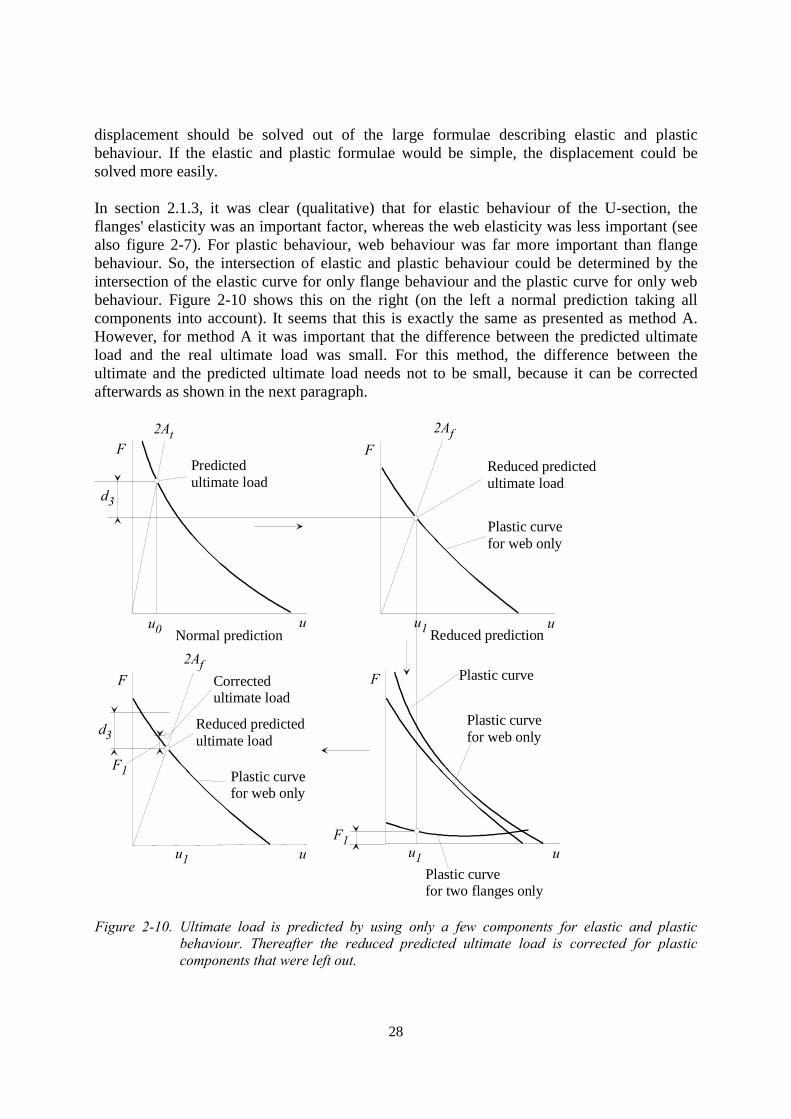
28
displacement should be solved out of the large formulae describing elastic and plasticbehaviour. If the elastic and plastic formulae would be simple, the displacement could besolved more easily.
In section 2.1.3, it was clear (qualitative) that for elastic behaviour of the U-section, theflanges' elasticity was an important factor, whereas the web elasticity was less important (seealso figure 2-7). For plastic behaviour, web behaviour was far more important than flangebehaviour. So, the intersection of elastic and plastic behaviour could be determined by theintersection of the elastic curve for only flange behaviour and the plastic curve for only webbehaviour. Figure 2-10 shows this on the right (on the left a normal prediction taking allcomponents into account). It seems that this is exactly the same as presented as method A.However, for method A it was important that the difference between the predicted ultimateload and the real ultimate load was small. For this method, the difference between theultimate and the predicted ultimate load needs not to be small, because it can be correctedafterwards as shown in the next paragraph.
u
FPredictedultimate load
Normal predictionu
F2Af
Plastic curvefor web only
Reduced prediction
Reduced predictedultimate load
d3
u1
u
F Plastic curve
Plastic curvefor web only
Plastic curvefor two flanges only
u1
F1
2At
u
F2Af
Plastic curvefor web only
Reduced predictedultimate load
u1
F1
Correctedultimate load
u0
d3
Figure 2-10. Ultimate load is predicted by using only a few components for elastic and plasticbehaviour. Thereafter the reduced predicted ultimate load is corrected for plasticcomponents that were left out.
29
The ultimate load was predicted by the intersection of an elastic and plastic curve using onlythe most contributing components. This predicted load will be defined as "Reduced predictedultimate load". Figure 2-10 shows that the plastic curves for the web or the two flanges areknown (figure 2-8 present these). It is possible to find out for u1 (the deformation at reducedpredicted ultimate load) which plastic load is needed to deform the two flanges F1. Theplastic behaviour of the flanges was not taken into account during the prediction of theultimate load. Load F1 can be added to the reduced predicted ultimate load to correct for theplastic behaviour of the flanges.
Note that the correction does not restore accuracy completely. If the intersection between theelastic curve and the plastic curve was calculated for the complete plastic curve (allcomponents), u1 would equal u0, and thus load F1.would equal d3.
2.1.5 Mathematical techniques
In section 2.1.3, components were presented. Each component was described by a formula.These formulae can be simplified by mathematical techniques like sensitivity analysis,rewriting of formulae, etc. In the next few paragraphs, these mathematical techniques will beintroduced. The mathematical techniques are coded by the character 'M' and a sequentialnumber.
M1: removing small terms in defined variable spaceThis technique makes it possible to remove certain terms in a formula because for all possiblevalues of variables, these terms do not have significant influence on the formula output. Apossible formula for a component is:
),(),(),(),,( zxizyhyxgzyxf ++= (2.2)
Because the variables x, y, and z have a practical meaning, (for instance x could be the platethickness), their values will be restricted to practical values as follows:
bxa << (2.3)
dyc << (2.4)
fze << (2.5)
This set of constrains (formula 2.3 to 2.5) is defined as a defined variable space. Changing x,y, and z between their minimal and maximal values, the value for the functions g, h, and i canbe calculated. Figure 2-11 presents these values.
Function f should be simplified within the defined variable space and function g, h, or i shouldbe removed. Figure 2-11 shows clearly that function i can be removed more easily thanfunctions g or h. Thus the simplified function will be:
),(),(),,( zyhyxgzyxf += (2.6)
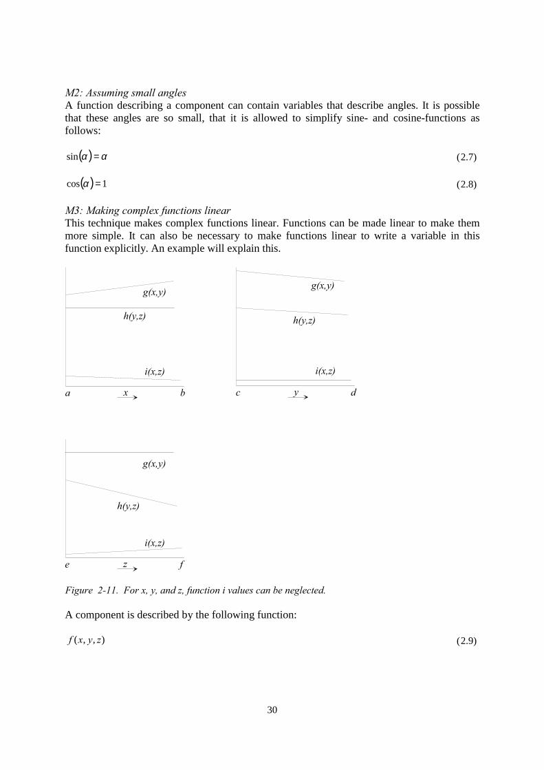
30
M2: Assuming small anglesA function describing a component can contain variables that describe angles. It is possiblethat these angles are so small, that it is allowed to simplify sine- and cosine-functions asfollows:
( ) αα =sin (2.7)
( ) 1cos =α (2.8)
M3: Making complex functions linearThis technique makes complex functions linear. Functions can be made linear to make themmore simple. It can also be necessary to make functions linear to write a variable in thisfunction explicitly. An example will explain this.
g(x,y)
h(y,z)
i(x,z)
a bx
g(x,y)
h(y,z)
i(x,z)
c dy
g(x,y)
h(y,z)
i(x,z)
e fz
Figure 2-11. For x, y, and z, function i values can be neglected.
A component is described by the following function:
),,( zyxf (2.9)
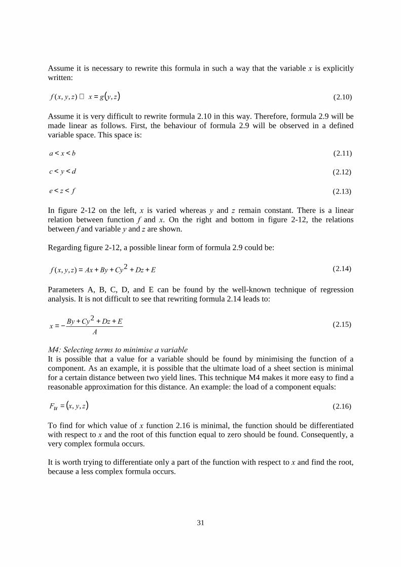
31
Assume it is necessary to rewrite this formula in such a way that the variable x is explicitlywritten:
( )zygxzyxf ,),,( =⇔ (2.10)
Assume it is very difficult to rewrite formula 2.10 in this way. Therefore, formula 2.9 will bemade linear as follows. First, the behaviour of formula 2.9 will be observed in a definedvariable space. This space is:
bxa << (2.11)
dyc << (2.12)
fze << (2.13)
In figure 2-12 on the left, x is varied whereas y and z remain constant. There is a linearrelation between function f and x. On the right and bottom in figure 2-12, the relationsbetween f and variable y and z are shown.
Regarding figure 2-12, a possible linear form of formula 2.9 could be:
EDzCyByAxzyxf ++++= 2),,( (2.14)
Parameters A, B, C, D, and E can be found by the well-known technique of regressionanalysis. It is not difficult to see that rewriting formula 2.14 leads to:
AEDzCyByx +++−=
2(2.15)
M4: Selecting terms to minimise a variableIt is possible that a value for a variable should be found by minimising the function of acomponent. As an example, it is possible that the ultimate load of a sheet section is minimalfor a certain distance between two yield lines. This technique M4 makes it more easy to find areasonable approximation for this distance. An example: the load of a component equals:
( )zyxuF ,,= (2.16)
To find for which value of x function 2.16 is minimal, the function should be differentiatedwith respect to x and the root of this function equal to zero should be found. Consequently, avery complex formula occurs.
It is worth trying to differentiate only a part of the function with respect to x and find the root,because a less complex formula occurs.
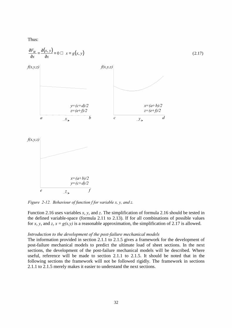
32
Thus:
( ) ( )yxgxx
yxxuF
,0, =⇔=∂
∂=∂
∂(2.17)
f(x,y,z)
y=(c+d)/2z=(e+f)/2
a bx
f(x,y,z)
x=(a+b)/2z=(e+f)/2
c dy
f(x,y,z)
x=(a+b)/2y=(c+d)/2
e fz
Figure 2-12. Behaviour of function f for variable x, y, and z.
Function 2.16 uses variables x, y, and z. The simplification of formula 2.16 should be tested inthe defined variable-space (formula 2.11 to 2.13). If for all combinations of possible valuesfor x, y, and z, x = g(x,y) is a reasonable approximation, the simplification of 2.17 is allowed.
Introduction to the development of the post-failure mechanical modelsThe information provided in section 2.1.1 to 2.1.5 gives a framework for the development ofpost-failure mechanical models to predict the ultimate load of sheet sections. In the nextsections, the development of the post-failure mechanical models will be described. Whereuseful, reference will be made to section 2.1.1 to 2.1.5. It should be noted that in thefollowing sections the framework will not be followed rigidly. The framework in sections2.1.1 to 2.1.5 merely makes it easier to understand the next sections.
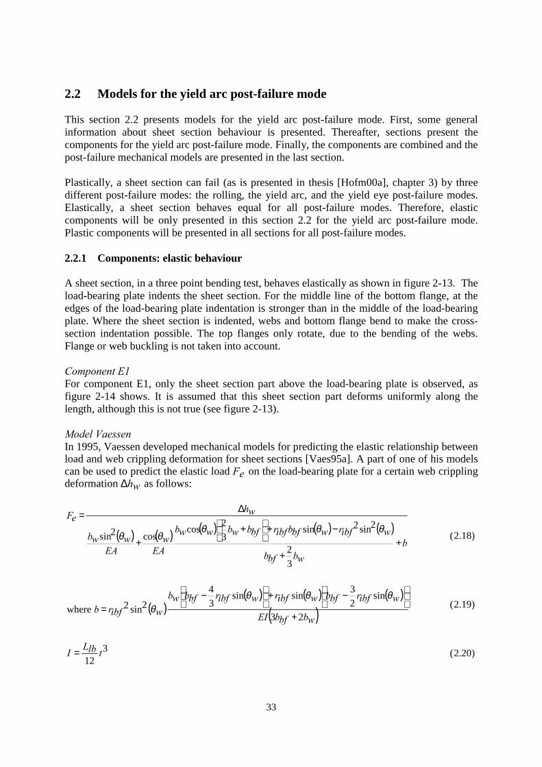
33
2.2 Models for the yield arc post-failure mode
This section 2.2 presents models for the yield arc post-failure mode. First, some generalinformation about sheet section behaviour is presented. Thereafter, sections present thecomponents for the yield arc post-failure mode. Finally, the components are combined and thepost-failure mechanical models are presented in the last section.
Plastically, a sheet section can fail (as is presented in thesis [Hofm00a], chapter 3) by threedifferent post-failure modes: the rolling, the yield arc, and the yield eye post-failure modes.Elastically, a sheet section behaves equal for all post-failure modes. Therefore, elasticcomponents will be only presented in this section 2.2 for the yield arc post-failure mode.Plastic components will be presented in all sections for all post-failure modes.
2.2.1 Components: elastic behaviour
A sheet section, in a three point bending test, behaves elastically as shown in figure 2-13. Theload-bearing plate indents the sheet section. For the middle line of the bottom flange, at theedges of the load-bearing plate indentation is stronger than in the middle of the load-bearingplate. Where the sheet section is indented, webs and bottom flange bend to make the cross-section indentation possible. The top flanges only rotate, due to the bending of the webs.Flange or web buckling is not taken into account.
Component E1For component E1, only the sheet section part above the load-bearing plate is observed, asfigure 2-14 shows. It is assumed that this sheet section part deforms uniformly along thelength, although this is not true (see figure 2-13).
Model VaessenIn 1995, Vaessen developed mechanical models for predicting the elastic relationship betweenload and web crippling deformation for sheet sections [Vaes95a]. A part of one of his modelscan be used to predict the elastic load Fe on the load-bearing plate for a certain web cripplingdeformation ∆hw as follows:
( ) ( ) ( ) ( ) ( )b
wbbfb
wibfrwbfbibfrbfbwbwwb
EAw
EAwwb
wheF
++
−+
+
+
∆=
32
2sin2sin32cos
cos2sinθθθ
θθ (2.18)
( )( ) ( ) ( )
( )wbbfbEI
wibfrbfbwibfrwibfrbfbwbwibfrb
23
sin23sinsin
34
2sin2 where+
−+
−
=θθθ
θ (2.19)
312
tlbLI = (2.20)
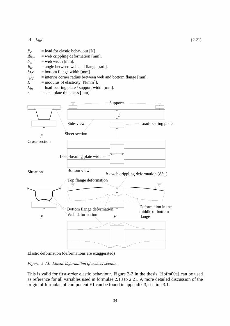
34
tlbLA = (2.21)
Fe = load for elastic behaviour [N].∆hw = web crippling deformation [mm].bw = web width [mm].θw = angle between web and flange [rad.].bbf = bottom flange width [mm].ribf = interior corner radius between web and bottom flange [mm].E = modulus of elasticity [N/mm2].Llb = load-bearing plate / support width [mm].t = steel plate thickness [mm].
F
F
Situation
Elastic deformation (deformations are exaggerated)
F F
F
Load-bearing plate
Sheet section
Supports
Cross-section
Bottom view
Side-view
Bottom flange deformation
Top flange deformation
Web deformation
h
h - web crippling deformation (∆hw)
Load-bearing plate width
Deformation in themiddle of bottomflange
Figure 2-13. Elastic deformation of a sheet section.
This is valid for first-order elastic behaviour. Figure 3-2 in the thesis [Hofm00a] can be usedas reference for all variables used in formulae 2.18 to 2.21. A more detailed discussion of theorigin of formulae of component E1 can be found in appendix 3, section 3.1.
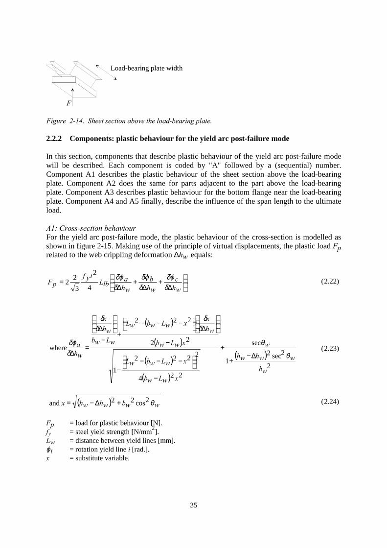
35
F
Load-bearing plate width
Figure 2-14. Sheet section above the load-bearing plate.
2.2.2 Components: plastic behaviour for the yield arc post-failure mode
In this section, components that describe plastic behaviour of the yield arc post-failure modewill be described. Each component is coded by "A" followed by a (sequential) number.Component A1 describes the plastic behaviour of the sheet section above the load-bearingplate. Component A2 does the same for parts adjacent to the part above the load-bearingplate. Component A3 describes plastic behaviour for the bottom flange near the load-bearingplate. Component A4 and A5 finally, describe the influence of the span length to the ultimateload.
A1: Cross-section behaviourFor the yield arc post-failure mode, the plastic behaviour of the cross-section is modelled asshown in figure 2-15. Making use of the principle of virtual displacements, the plastic load Fprelated to the web crippling deformation ∆hw equals:
∆
+∆
+∆
=whc
whb
wha
lbLtyf
pFδδϕ
δδϕ
δδϕ
4
2
322 (2.22)
( )
( )
( )
( )
( )
2
2sec21
sec
224
2222
1
22
222
where
wbwwhwh
w
xwLwb
xwLwbwL
xwLwb
whxxwLwbwL
wLwbwh
x
wha
θ
θ
δδ
δδ
δδϕ
∆−+
+
−
−−−−
−
∆
−−−
+−
∆
=∆
(2.23)
( ) wwbwhwhx θ2cos22 and +∆−= (2.24)
Fp = load for plastic behaviour [N].fy = steel yield strength [N/mm2].Lw = distance between yield lines [mm].ϕi = rotation yield line i [rad.].x = substitute variable.
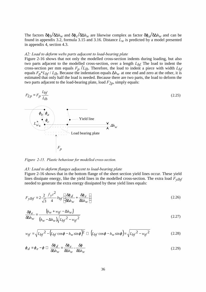
36
The factors δϕb/δ∆hw and δϕc/δ∆hw are likewise complex as factor δϕa/δ∆hw and can befound in appendix 3.2, formula 3.15 and 3.16. Distance Lw is predicted by a model presentedin appendix 4, section 4.3.
A2: Load to deform webs parts adjacent to load-bearing plateFigure 2-16 shows that not only the modelled cross-section indents during loading, but alsotwo parts adjacent to the modelled cross-section, over a length Lbf. The load to indent thecross-section per mm equals Fp /Llb. Therefore, the load to indent a piece with width Lbfequals Fp*Lbf / Llb. Because the indentation equals ∆hw at one end and zero at the other, it isestimated that only half the load is needed. Because there are two parts, the load to deform thetwo parts adjacent to the load-bearing plate, load F2p, simply equals:
lbLbfL
pFpF =2 (2.25)
Load bearing plate
Yield line
Fp
∆hw
ϕaϕbϕcLw
Figure 2-15. Plastic behaviour for modelled cross-section.
A3: Load to deform flanges adjacent to load-bearing plateFigure 2-16 shows that in the bottom flange of the sheet section yield lines occur. These yieldlines dissipate energy, like the yield lines in the modelled cross-section. The extra load Fylbfneeded to generate the extra energy dissipated by these yield lines equals:
∆
+∆
=whe
whd
bfbtyf
ylbfFδδϕ
δδϕ
4
2
322 (2.26)
( )( )
22
tfwbfLwhwh
whtfwwh
whe
−∆−
∆−+=
∆δδϕ
(2.27)
( ) ( ) 22sincos2sincos2tfwbfLwhbfLwhbfLbfLtfw −=−⇔−−= ϕϕϕϕ (2.28)
whwhe
whded ∆∆
=∆
⇔−=δ
δϕδδϕ
δδϕϕϕϕ - (2.29)
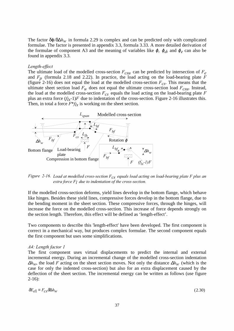
37
The factor δϕ/δ∆hw in formula 2.29 is complex and can be predicted only with complicatedformulae. The factor is presented in appendix 3.3, formula 3.33. A more detailed derivation ofthe formulae of component A3 and the meaning of variables like ϕ, ϕd, and ϕe can also befound in appendix 3.3.
Length-effectThe ultimate load of the modelled cross-section Fcsu can be predicted by intersection of Feand Fp (formula 2.18 and 2.22). In practice, the load acting on the load-bearing plate F(figure 2-16) does not equal the load at the modelled cross-section Fcs. This means that theultimate sheet section load Fu does not equal the ultimate cross-section load Fcsu. Instead,the load at the modelled cross-section Fcs equals the load acting on the load-bearing plate Fplus an extra force (flx-1)F due to indentation of the cross-section. Figure 2-16 illustrates this.Then, in total a force F*flx is working on the sheet section.
Load-bearingplate
Rotation ϕ
Bottom flange
Compression in bottom flange
F
F
Lspan
(flx-1)FFbf
Lbf ∆hw
LbfFbf
∆hwFbf
FcsLlb
Modelled cross-section
Figure 2-16. Load at modelled cross-section Fcs equals load acting on load-bearing plate F plus anextra force Fl due to indentation of the cross-section.
If the modelled cross-section deforms, yield lines develop in the bottom flange, which behavelike hinges. Besides these yield lines, compressive forces develop in the bottom flange, due tothe bending moment in the sheet section. These compressive forces, through the hinges, willincrease the force on the modelled cross-section. This increase of force depends strongly onthe section length. Therefore, this effect will be defined as ‘length-effect’.
Two components to describe this 'length-effect' have been developed. The first component iscorrect in a mechanical way, but produces complex formulae. The second component equalsthe first component but uses some simplifications.
A4: Length factor 1The first component uses virtual displacements to predict the internal and externalincremental energy. During an incremental change of the modelled cross-section indentation∆hw, the load F acting on the sheet section moves. Not only the distance ∆hw (which is thecase for only the indented cross-section) but also for an extra displacement caused by thedeflection of the sheet section. The incremental energy can be written as follows (use figure2-16):
whcsFeE ∆= δδ 1 (2.30)
38
−+∆=
22lbLspanL
whFeE δϕδδ (2.31)
δEe1 = incremental external energy cross-section only.δEe2 = incremental external energy cross-section and sheet section deflection.δ∆hw = incremental modelled cross-section indentation.δϕ = incremental sheet section rotation.
Influences of stress on yield line energy dissipation are neglected and it is assumed that theyield line pattern does not change geometrically during deformation. Then, because bothmentioned external energy terms should equal the incremental internal energy and internalenergy is equal for both cases, it can be derived that:
⇔= 21 eEeE δδ
⇔
−+∆
∆=⇔
−+∆=∆
2
2 lbLspanLwh
whcsFFlbLspanL
whFwhcsF
δϕδ
δδϕδδ
1*
21
1lfcsF
lbLspanL
wh
csFF =
−
∆+
=
δδϕ (2.32)
fl1 = length factor 1
The factor δϕ/δ∆hw is complex and can be predicted only with complicated formulae. This isshown in appendix 3.3, formula 3.33.
A5: Length factor 2A part of length factor 1 can be simplified, avoiding the complex calculating of factorδϕ/δ∆hw. Formula 3.33 is here presented:
( )whwhtfwbfL
tfw
wh ∆−−=
∆ 22δδϕ
(3.33)
If it is assumed that wtf equals approximately ∆hw (see figure 3-2), this formula 3.33 can besimplified into:
( )whwhwhbfL
wh
wh ∆−∆−
∆=
∆ 22δδϕ
(2.33)
39
Then, length factor 2 is described by the formula:
( )
2*
2221
1lfcsF
lbLspanL
whwhwhLbf
whcsFF =
−
∆−∆−
∆+
=
(2.34)
Summary of loadsThe modelled cross-section is loaded during elastic behaviour by Fe (formulae 2.18 to 2.21)and during plastic behaviour by Fp (formulae 2.22 to 2.24). The two curves of Fe and Fpform an envelope for the behaviour of the modelled cross-section for load Fcs. The ultimateload of the cross-section equals Fcsu.
Besides the load Fcsu to indent the modelled cross-section, other loads are needed for thewhole sheet section. The load F2p (formula 2.25) to deform the two web parts adjacent to themodelled cross-section and the load Fylbf (formulae 2.26 to 2.29) to deform the bottomflange.
Due to the interaction between bending moment and concentrated load, Fcs will becomesmaller, resulting in a force Fcs *fl1 or Fcs *fl2 (formulae 2.32 and 2.34).
Determination of yield line distancesAll the forces of the previous paragraph result in the load at which the section fails Fu. Theonly problem is the unknown values of Lbf and Lw (figure 2-16 and 2-15). Distance Lbf canbe found by minimisation of the load Fu. Regarding formulae 2.18 to 2.32, which are allneeded to predict Fu, it will be clear that this minimisation leads to many complex formulae.Therefore, simplified formulae will be derived of formulae 2.18 to 2.32 in the next section,where after it is possible to determine Lbf. Distance Lw can be found by a mechanical modelin appendix 4, section 4.3.
2.2.3 Prediction of the ultimate load using components
IntroductionSection 2.1 presented the methodology used in this appendix to develop post-failuremechanical models to predict the ultimate load for sheet sections. For the yield arc post-failure mode, section 2.2.1 and 2.2.2 presented components that can be used to describeelastic and plastic curves. Now, these components and mathematical techniques (presented inparagraph 2.1.5) will be used to develop the post-failure mechanical models that predict theultimate load for the yield arc post-failure mode. The mechanical models will have a code thatmakes them easily recognisable. The character "M" stands for model, "A" for the yield arcpost-failure mode and, later, "R" for the rolling post-failure mode and "E" for the yield eyepost-failure mode.
In this appendix 2, many derivations made for developing the post-failure models will only bebriefly discussed. Appendix 3 will present derivations with full details.
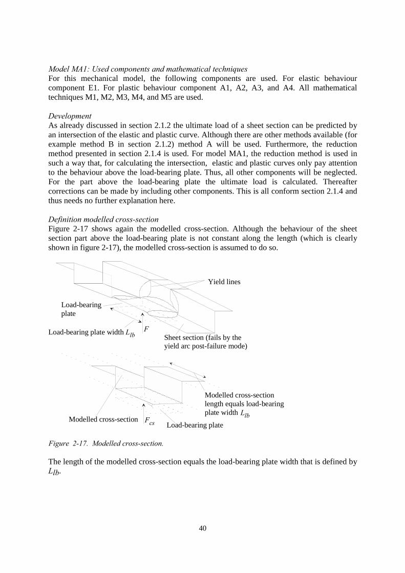
40
Model MA1: Used components and mathematical techniquesFor this mechanical model, the following components are used. For elastic behaviourcomponent E1. For plastic behaviour component A1, A2, A3, and A4. All mathematicaltechniques M1, M2, M3, M4, and M5 are used.
DevelopmentAs already discussed in section 2.1.2 the ultimate load of a sheet section can be predicted byan intersection of the elastic and plastic curve. Although there are other methods available (forexample method B in section 2.1.2) method A will be used. Furthermore, the reductionmethod presented in section 2.1.4 is used. For model MA1, the reduction method is used insuch a way that, for calculating the intersection, elastic and plastic curves only pay attentionto the behaviour above the load-bearing plate. Thus, all other components will be neglected.For the part above the load-bearing plate the ultimate load is calculated. Thereaftercorrections can be made by including other components. This is all conform section 2.1.4 andthus needs no further explanation here.
Definition modelled cross-sectionFigure 2-17 shows again the modelled cross-section. Although the behaviour of the sheetsection part above the load-bearing plate is not constant along the length (which is clearlyshown in figure 2-17), the modelled cross-section is assumed to do so.
Sheet section (fails by theyield arc post-failure mode)
Load-bearingplate
Yield lines
Modelled cross-sectionLoad-bearing plate
Load-bearing plate width Llb
Modelled cross-sectionlength equals load-bearingplate width
Fcs
F
Llb
Figure 2-17. Modelled cross-section.
The length of the modelled cross-section equals the load-bearing plate width that is defined byLlb.
41
Intersection of E1 and A1If the modelled cross-section as shown in figure 2-17 behaves elastically, formulae 2.18 to2.21 yield. Using mathematical technique M1, (paragraph 2.1.5) formulae 2.18 to 2.21 arereduced to:
( )( ) ( )
−
∆+=
wibfrbfbwbwibfr
whwbbfbEIeF
θθ sin342sin2
23(2.35)
Details are presented in appendix 3, section 3.5, formulae 3.69 to 3.77. Mathematicaltechnique M1 uses a defined variable space. In this case, the variable space is defined asvariable space A as follows:
15050 << wb [mm]. (2.36)
9050 << wθ [degrees]. (2.37)
15050 << lbL [mm]. (2.38)
5.15.0 << t [mm]. (2.39)
15040 << bfb [mm]. (2.40)
121 << bfr [mm]. (2.41)
101.0 <∆< wh [mm]. (2.42)
Using techniques M3 and M1 for variable space A, formula 2.22, 2.23, and 2.24 can bereduced. Setting equal the reduced formulae to formula 2.35 yields to the predicted ultimateload of the modelled cross-section. This load is defined as Fcsu. Details are presented inappendix 3.6, formulae 3.78 to 3.93.
( ) ( )( ) wLwLwbA
kwLwLwbwhAcsuF
−++−+−−
=2
24 αβαβα (2.43)
( )( ) ( )
sin
342sin2
23
−
+=
wbfrbfbwbwibfr
wbbfbEIk
θθ (2.44)
2tlbLyf=α (2.45)
( )( ) wLwbwBLCwkL −+=β (2.46)
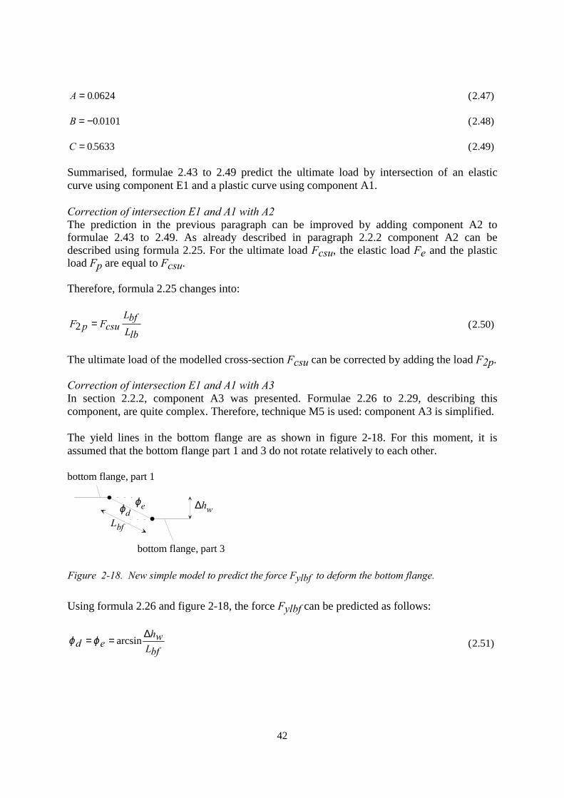
42
06240.A = (2.47)
01010.B −= (2.48)
56330.C = (2.49)
Summarised, formulae 2.43 to 2.49 predict the ultimate load by intersection of an elasticcurve using component E1 and a plastic curve using component A1.
Correction of intersection E1 and A1 with A2The prediction in the previous paragraph can be improved by adding component A2 toformulae 2.43 to 2.49. As already described in paragraph 2.2.2 component A2 can bedescribed using formula 2.25. For the ultimate load Fcsu, the elastic load Fe and the plasticload Fp are equal to Fcsu.
Therefore, formula 2.25 changes into:
lbLbfL
csuFpF =2 (2.50)
The ultimate load of the modelled cross-section Fcsu can be corrected by adding the load F2p.
Correction of intersection E1 and A1 with A3In section 2.2.2, component A3 was presented. Formulae 2.26 to 2.29, describing thiscomponent, are quite complex. Therefore, technique M5 is used: component A3 is simplified.
The yield lines in the bottom flange are as shown in figure 2-18. For this moment, it isassumed that the bottom flange part 1 and 3 do not rotate relatively to each other.
Lbf
∆hwϕdϕe
bottom flange, part 1
bottom flange, part 3
Figure 2-18. New simple model to predict the force Fylbf to deform the bottom flange.
Using formula 2.26 and figure 2-18, the force Fylbf can be predicted as follows:
bfLwh
ed∆
== arcsinϕϕ (2.51)
43
221
21
1
whbfL
bfLwh
bfLwhe
whd
∆−=
∆−
=∆
=∆ δ
δϕδδϕ
(2.52)
∆
+∆
=whe
whd
bfbtyf
ylbfFδδϕ
δδϕ
4
2
322 (2.26)
The ultimate load of the modelled cross-section Fcsu can be corrected by adding the loadFylbf.
Correction intersection E1 and A1 with A4In section 2.2.2 component A4 was presented. If mathematical technique M2 (section 2.1.5) isused with variable angle ϕ in formula 2.28 component A4 can be rewritten as:
( )( )( )whwhwhbfL
whbfLbfLlbLspanLlf
∆−−
−−
−+
=
ϕ
ϕ 22
21
11
(2.53)
Web crippling deformation ∆hw was calculated by formulae 3.88 and 3.89 for finding Fcsu informula 2.34. Rotation ϕ can be calculated by formula 3.97, appendix 3.7.
Further details are presented in appendix 3.7, formulae 3.94 to 3.99. Using this length factorfl1 (component A4), the ultimate load of the sheet section can be calculated as follows:
( ) 12 lfylbfFpFcsuFuF ++= (2.54)
Finding yield line distance LbfThe distance between yield lines Lbf is shown in figure 2-16. The distance Lbf can bedetermined by varying Lbf and finding the minimum value for the ultimate load Fu (formula2.54). To differentiate formula 2.54 to Lbf and find the root is difficult. Therefore,mathematical technique M4 is used. If only Fcsu, F2p and Fylbf of formula 2.54 are used, thefollowing equation should be solved. Details are presented in appendix 3.8, formulae 3.100 to3.110.
02 =
∂
∂+
∂
∂+
∂∂=
∂∂
bfLylbfF
bfLpF
bfLcsuF
bfLuF
(2.55)
Note that the correct equation should be:
( ) 0121
2 =∂∂
+++
∂
∂+
∂
∂+
∂∂
=∂∂
bfLlf
ylbfFpFcsuFlfbfL
ylbfF
bfLpF
bfLcsuF
bfLuF
(2.56)
44
Equation 2.55 can be solved easily. The result equals:
csuFbfblbLtyf
bfL4
601.222= (2.57)
2.2.4 Overview of formulae
In this section, an overview of formulae needed to use model MA1 is given. If all formulaeare used in sequence, a prediction of the ultimate load of a sheet section results.
First, calculate the ultimate load of the modelled cross-section:
( ) ( )( ) wLwLwbA
kwLwLwbwhAcsuF
−++−+−−
2
24 αβαβα (2.43)
( )
sin342sin2
23
−
+=
wbfrbfbwbwbfr
wbbfbEIk
θθ(2.44)
2tlbLyf=α (2.45)
( )( ) wLwbwBLCwkL −+=β (2.46)
06240.A = (2.47)
01010.B −= (2.48)
56330.C = (2.49)
Distance Lw is predicted by a method presented in appendix 4, section 4.3. Now, yield linedistance Lbf can be calculated.
csuFbfblbLtyf
bfL4
601.222= (2.57)
Then F2p, Fylbf, and fl1 can be calculated:
lbLbfL
csuFpF =2 (2.50)
45
∆
+∆
=whe
whdbfb
tyfylbfF
δδϕ
δδϕ
4
22 (2.26)
221
21
1
whbfL
bfLwh
bfLwhe
whd
∆−=
∆−
=∆
=∆ δ
δϕδδϕ
(2.52)
The prediction of the ultimate load equals:
( ) 12 lfylbfFpFcsuFuF ++= (2.54)
With:
( )( )( )whwhwhbfL
whbfLbfLlbLspanLlf
∆−−
−−
−+
=
ϕ
ϕ 22
21
11
(2.53)
Web crippling deformation ∆hw was calculated by formulae 3.88 and 3.89 for finding Fcsu informula 2.34. Rotation ϕ can be calculated by formula 3.97, appendix 3.7.
2.2.5 Other models
Model MA2Model MA2 equals model MA1 with exception of component A2. This component is nottaken into account. This means that force F2p is removed from formula 2.54:
( ) 1lfylbfFcsuFuF += (2.58)
Model MA3Model MA3 equals model MA1 with exception of component A3. This component is nottaken into account. This means that force Fylbf is removed from formula 2.54:
( ) 12 lfpFcsuFuF += (2.59)
Model MA4Model MA4 equals model MA1 with exception of the components A2 and A3. Thesecomponents are not taken into account. This means that forces F2p and Fylbf are removedfrom formula 2.54:
1* lfcsuFuF = (2.60)
46
Model MA5Model MA5 equals model MA1 with exception of component A4. Instead of this component,component A5 is used. Component A5 is described by formula 2.34. Formula 2.54 changesinto:
( ) 22 lfylbfFpFcsuFuF ++= (2.61)
Model MA6Model MA6 equals model MA5 with exception of component A2. This component is nottaken into account. This means that force F2p is removed from formula 2.61:
( ) 2lfylbfFcsuFuF += (2.62)
Model MA7Model MA7 equals model MA5 with exception of component A3. This component is nottaken into account. This means that force Fylbf is removed from formula 2.61:
( ) 22 lfpFcsuFuF += (2.63)
Model MA8Model MA8 equals model MA5 with exception of the components A2 and A4. Thesecomponents are not taken into account. This means that forces F2p and Fylbf are removedfrom formula 2.61:
2* lfcsuFuF = (2.64)
Model MA9Model MA9 equals model MA1 with exception of component A5. This component isremoved and is not replaced by an other component. This means that the length factor fl1 isremoved from formula 2.54:
ylbfFpFcsuFuF ++= 2 (2.65)
Model MA10Model MA10 equals model MA9 with exception of component A2. This component is nottaken into account. This means that force F2p is removed from formula 2.65:
ylbfFcsuFuF += (2.66)
Model MA11Model MA11 equals model MA9 with exception of component A3. This component is nottaken into account. This means that force Fylbf is removed from formula 2.65:
pFcsuFuF 2+= (2.67)

47
Model MA12Model MA12 equals model MA9 with exception of the components A2 and A3. Thesecomponents are not taken into account. This means that forces F2p and Fylbf are removedfrom formula 2.65:
csuFuF = (2.68)
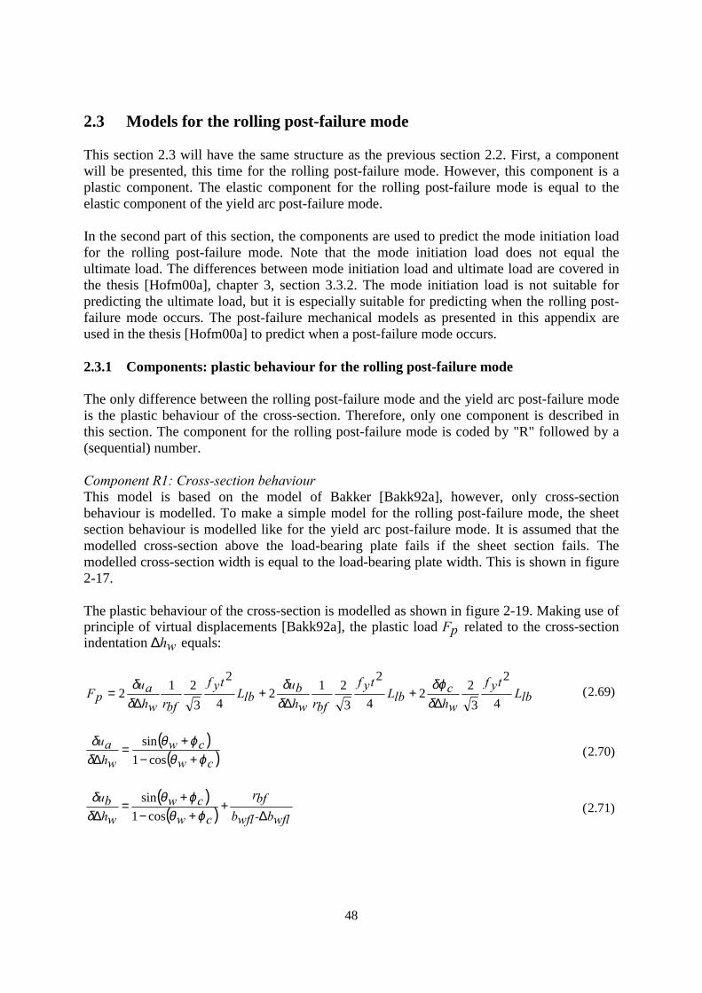
48
2.3 Models for the rolling post-failure mode
This section 2.3 will have the same structure as the previous section 2.2. First, a componentwill be presented, this time for the rolling post-failure mode. However, this component is aplastic component. The elastic component for the rolling post-failure mode is equal to theelastic component of the yield arc post-failure mode.
In the second part of this section, the components are used to predict the mode initiation loadfor the rolling post-failure mode. Note that the mode initiation load does not equal theultimate load. The differences between mode initiation load and ultimate load are covered inthe thesis [Hofm00a], chapter 3, section 3.3.2. The mode initiation load is not suitable forpredicting the ultimate load, but it is especially suitable for predicting when the rolling post-failure mode occurs. The post-failure mechanical models as presented in this appendix areused in the thesis [Hofm00a] to predict when a post-failure mode occurs.
2.3.1 Components: plastic behaviour for the rolling post-failure mode
The only difference between the rolling post-failure mode and the yield arc post-failure modeis the plastic behaviour of the cross-section. Therefore, only one component is described inthis section. The component for the rolling post-failure mode is coded by "R" followed by a(sequential) number.
Component R1: Cross-section behaviourThis model is based on the model of Bakker [Bakk92a], however, only cross-sectionbehaviour is modelled. To make a simple model for the rolling post-failure mode, the sheetsection behaviour is modelled like for the yield arc post-failure mode. It is assumed that themodelled cross-section above the load-bearing plate fails if the sheet section fails. Themodelled cross-section width is equal to the load-bearing plate width. This is shown in figure2-17.
The plastic behaviour of the cross-section is modelled as shown in figure 2-19. Making use ofprinciple of virtual displacements [Bakk92a], the plastic load Fp related to the cross-sectionindentation ∆hw equals:
lbLtyf
whc
lbLtyf
bfrwhbu
lbLtyf
bfrwhau
pF4
2
322
4
2
3212
4
2
3212
∆+
∆+
∆=
δδϕ
δδ
δδ (2.69)
( )( ) cos1
sin
cwcw
whau
ϕθϕθ
δδ
+−+
=∆ (2.70)
( )( ) wflb-wflb
bfr
cwcw
whbu
∆+
+−+
=∆ ϕθ
ϕθδδ
cos1sin
(2.71)
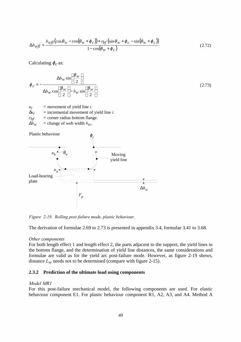
49
( )( ) ( )( )( )cw
cwcwbfrcwwwflbwflb
ϕθϕθϕθϕθθ
+−
+−+++−=∆
cos1sinsincoscos
(2.72)
Calculating ϕc as:
−
∆
∆
−=
2sin
2cos
2sin
wwbw
wh
wwh
c θθ
θ
ϕ (2.73)
ui = movement of yield line i.δui = incremental movement of yield line i.rbf = corner radius bottom flange.∆bw = change of web width bw..
Load-bearingplate
Plastic behaviour
Movingyield line
∆hwFp
ua
ub θw
ϕc
Figure 2-19. Rolling post-failure mode, plastic behaviour.
The derivation of formulae 2.69 to 2.73 is presented in appendix 3.4, formulae 3.41 to 3.68.
Other componentsFor both length effect 1 and length effect 2, the parts adjacent to the support, the yield lines inthe bottom flange, and the determination of yield line distances, the same considerations andformulae are valid as for the yield arc post-failure mode. However, as figure 2-19 shows,distance Lw needs not to be determined (compare with figure 2-15).
2.3.2 Prediction of the ultimate load using components
Model MR1For this post-failure mechanical model, the following components are used. For elasticbehaviour component E1. For plastic behaviour component R1, A2, A3, and A4. Method A
50
mentioned in section 2.1.2 is used to predict the ultimate load. All mathematical techniquesM1, M2, M3, M4, and M5 will be used.
Equal to model MA1, this model MR1, predicting the ultimate load for the rolling post-failuremode, will be based on the reduction method presented in section 2.1.4. The ultimate load ispredicted by intersection of an elastic and plastic curve. These curves pay only attention to themodelled cross-section section (the part above the load-bearing plate, defined in section 2.2.3,figure 2-17).
For the elastic curve, component E1 describes the behaviour of the modelled cross-section.The plastic curve for the modelled cross-section is described by component R1.
After the prediction of the ultimate load of the modelled cross-section, the predicted ultimateload is corrected. This correction is carried out using components that describe the behaviourof parts adjacent to the load-bearing plate or components describing a length effect. For theyield arc and rolling post-failure modes, these components are equal. This means the ultimateload prediction for the rolling post-failure mode is corrected with the same components as forthe model MA1: the components A2, A3, and A4.
Intersection of E1 and R1If the modelled cross-section as shown in figure 2-17 behaves elastically formulae 2.18 to2.21 yield. Using mathematical technique M1, (paragraph 2.1.5) formulae 2.18 to 2.21 arereduced to:
( )( ) ( )
−
∆+=
wbfrbfbwbwbfr
whwbbfbEIeF
θθ sin342sin2
23(2.35)
Details are presented in appendix 3.5, formulae 3.69 to 3.77. Mathematical technique M1 usesa defined variable space. In this case, the variable space is defined as variable space A (seeformulae 2.36 to 2.42).
Using mathematical technique M1 for defined variable space A (formulae 2.36 to 2.42), theformulae describing the plastic behaviour for the rolling mechanism (2.69 to 2.73) can besimplified into:
( ) ( )( ) ( ) lbL
tyf
bfrwcwwcw
pF4
2
321
sincos1cossin
2*2θϕθ
θϕθ+−
+= (2.74)
Details are presented in appendix 3.9, formulae 3.111 to 3.121. Now, the elastic (formula2.35) and plastic load (formula 2.74) of the modelled cross-section can be set equal.Consequently, the predicted ultimate load Fcsu of the modelled cross-section can be solved(appendix 3.9, formulae 3.111 to 3.121):
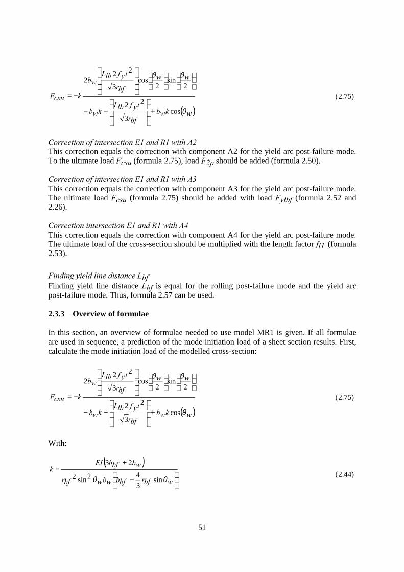
51
( )
cos3
22
2sin
2cos
3
222
wkwbbfr
tyflbLkwb
wwbfr
tyflbLwb
kcsuF
θ
θθ
+
−−
−= (2.75)
Correction of intersection E1 and R1 with A2This correction equals the correction with component A2 for the yield arc post-failure mode.To the ultimate load Fcsu (formula 2.75), load F2p should be added (formula 2.50).
Correction of intersection E1 and R1 with A3This correction equals the correction with component A3 for the yield arc post-failure mode.The ultimate load Fcsu (formula 2.75) should be added with load Fylbf (formula 2.52 and2.26).
Correction intersection E1 and R1 with A4This correction equals the correction with component A4 for the yield arc post-failure mode.The ultimate load of the cross-section should be multiplied with the length factor fl1 (formula2.53).
Finding yield line distance LbfFinding yield line distance Lbf is equal for the rolling post-failure mode and the yield arcpost-failure mode. Thus, formula 2.57 can be used.
2.3.3 Overview of formulae
In this section, an overview of formulae needed to use model MR1 is given. If all formulaeare used in sequence, a prediction of the mode initiation load of a sheet section results. First,calculate the mode initiation load of the modelled cross-section:
( )
cos3
22
2sin
2cos
3
222
wkwbbfr
tyflbLkwb
wwbfr
tyflbLwb
kcsuF
θ
θθ
+
−−
−= (2.75)
With:
( )
sin342sin2
23
−
+=
wbfrbfbwbwbfr
wbbfbEIk
θθ(2.44)
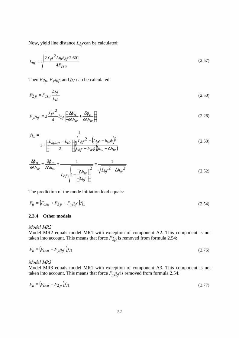
52
Now, yield line distance Lbf can be calculated:
csuFbfblbLtyf
bfL4
601.222= (2.57)
Then F2p, Fylbf, and fl1 can be calculated:
lbLbfL
csuFpF =2 (2.50)
∆
+∆
=whe
whdbfb
tyfylbfF
δδϕ
δδϕ
4
22 (2.26)
( )( )( )whwhwhbfL
whbfLbfLlbLspanLlf
∆−−
−−
−+
=
ϕ
ϕ 22
21
11
(2.53)
221
21
1
whbfL
bfLwh
bfLwhe
whd
∆−=
∆−
=∆
=∆ δ
δϕδδϕ
(2.52)
The prediction of the mode initiation load equals:
( ) 12 lfylbfFpFcsuFuF ++= (2.54)
2.3.4 Other models
Model MR2Model MR2 equals model MR1 with exception of component A2. This component is nottaken into account. This means that force F2p is removed from formula 2.54:
( ) 1lfylbfFcsuFuF += (2.76)
Model MR3Model MR3 equals model MR1 with exception of component A3. This component is nottaken into account. This means that force Fylbf is removed from formula 2.54:
( ) 12 lfpFcsuFuF += (2.77)
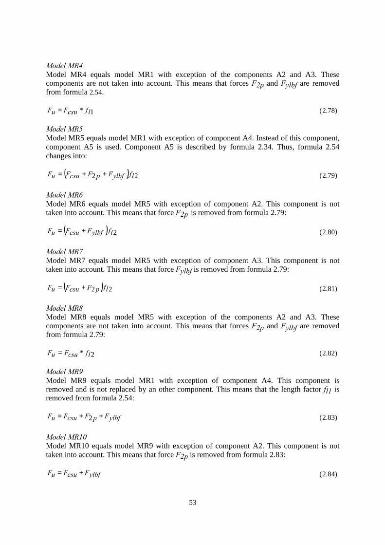
53
Model MR4Model MR4 equals model MR1 with exception of the components A2 and A3. Thesecomponents are not taken into account. This means that forces F2p and Fylbf are removedfrom formula 2.54.
1* lfcsuFuF = (2.78)
Model MR5Model MR5 equals model MR1 with exception of component A4. Instead of this component,component A5 is used. Component A5 is described by formula 2.34. Thus, formula 2.54changes into:
( ) 22 lfylbfFpFcsuFuF ++= (2.79)
Model MR6Model MR6 equals model MR5 with exception of component A2. This component is nottaken into account. This means that force F2p is removed from formula 2.79:
( ) 2lfylbfFcsuFuF += (2.80)
Model MR7Model MR7 equals model MR5 with exception of component A3. This component is nottaken into account. This means that force Fylbf is removed from formula 2.79:
( ) 22 lfpFcsuFuF += (2.81)
Model MR8Model MR8 equals model MR5 with exception of the components A2 and A3. Thesecomponents are not taken into account. This means that forces F2p and Fylbf are removedfrom formula 2.79:
2* lfcsuFuF = (2.82)
Model MR9Model MR9 equals model MR1 with exception of component A4. This component isremoved and is not replaced by an other component. This means that the length factor fl1 isremoved from formula 2.54:
ylbfFpFcsuFuF ++= 2 (2.83)
Model MR10Model MR10 equals model MR9 with exception of component A2. This component is nottaken into account. This means that force F2p is removed from formula 2.83:
ylbfFcsuFuF += (2.84)
54
Model MR11Model MR11 equals model MR9 with exception of component A3. This component is nottaken into account. This means that force Fylbf is removed from formula 2.83:
pFcsuFuF 2+= (2.85)
Model MR12Model MR12 equals model MR9 with exception of the components A2 and A3. Thesecomponents are not taken into account. This means that forces F2p and Fylbf are removedfrom formula 2.83:
csuFuF = (2.86)
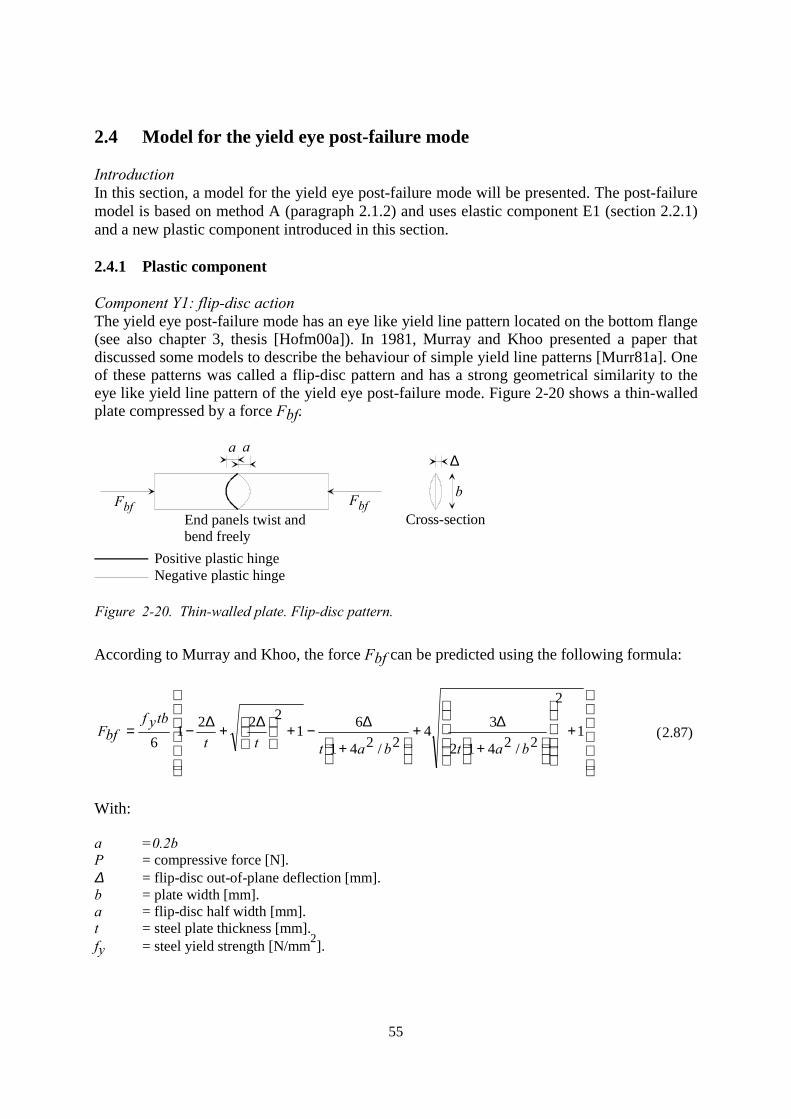
55
2.4 Model for the yield eye post-failure mode
IntroductionIn this section, a model for the yield eye post-failure mode will be presented. The post-failuremodel is based on method A (paragraph 2.1.2) and uses elastic component E1 (section 2.2.1)and a new plastic component introduced in this section.
2.4.1 Plastic component
Component Y1: flip-disc actionThe yield eye post-failure mode has an eye like yield line pattern located on the bottom flange(see also chapter 3, thesis [Hofm00a]). In 1981, Murray and Khoo presented a paper thatdiscussed some models to describe the behaviour of simple yield line patterns [Murr81a]. Oneof these patterns was called a flip-disc pattern and has a strong geometrical similarity to theeye like yield line pattern of the yield eye post-failure mode. Figure 2-20 shows a thin-walledplate compressed by a force Fbf.
Fbf
aa
End panels twist and bend freely
Positive plastic hingeNegative plastic hinge
∆
Cross-section
bFbf
Figure 2-20. Thin-walled plate. Flip-disc pattern.
According to Murray and Khoo, the force Fbf can be predicted using the following formula:
1
2
2/2412
342/241
612221
6
+
+
∆+
+
∆−+
∆+∆−=
batbattt
tbyfbfF (2.87)
With:
a =0.2bP = compressive force [N].∆ = flip-disc out-of-plane deflection [mm].b = plate width [mm].a = flip-disc half width [mm].t = steel plate thickness [mm].fy = steel yield strength [N/mm2].
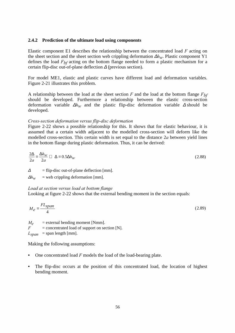
56
2.4.2 Prediction of the ultimate load using components
Elastic component E1 describes the relationship between the concentrated load F acting onthe sheet section and the sheet section web crippling deformation ∆hw. Plastic component Y1defines the load Fbf acting on the bottom flange needed to form a plastic mechanism for acertain flip-disc out-of-plane deflection ∆ (previous section).
For model ME1, elastic and plastic curves have different load and deformation variables.Figure 2-21 illustrates this problem.
A relationship between the load at the sheet section F and the load at the bottom flange Fbfshould be developed. Furthermore a relationship between the elastic cross-sectiondeformation variable ∆hw and the plastic flip-disc deformation variable ∆ should bedeveloped.
Cross-section deformation versus flip-disc deformationFigure 2-22 shows a possible relationship for this. It shows that for elastic behaviour, it isassumed that a certain width adjacent to the modelled cross-section will deform like themodelled cross-section. This certain width is set equal to the distance 2a between yield linesin the bottom flange during plastic deformation. Thus, it can be derived:
whawh
a∆=∆⇔
∆=∆ 5.0
222 (2.88)
∆ = flip-disc out-of-plane deflection [mm].∆hw = web crippling deformation [mm].
Load at section versus load at bottom flangeLooking at figure 2-22 shows that the external bending moment in the section equals:
4spanFL
eM = (2.89)
Me = external bending moment [Nmm].F = concentrated load of support on section [N].Lspan = span length [mm].
Making the following assumptions:
• One concentrated load F models the load of the load-bearing plate.
• The flip-disc occurs at the position of this concentrated load, the location of highestbending moment.
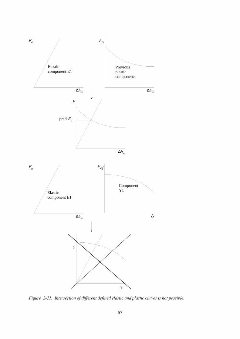
57
Fe Fp
∆hw
?
Fu
?
∆hw
∆hw
∆
ComponentY1
Elasticcomponent E1
Previousplasticcomponents
pred.
F
Fe
∆hw
Elasticcomponent E1
Fbf
Figure 2-21. Intersection of different defined elastic and plastic curves is not possible.
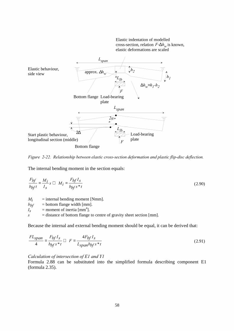
58
∆hw=h1-h2
Bottom flangeF
Lspan
Llb
Elastic indentation of modelledcross-section, relation is known,elastic deformations are scaled
2∆
Bottom flangeF
2a
Elastic behaviour,side view
Start plastic behaviour,longitudinal section (middle)
h1
h2approx. ∆hw
Llb
Lspan
Load-bearingplate
Load-bearingplate
F-∆hw
Figure 2-22. Relationship between elastic cross-section deformation and plastic flip-disc deflection.
The internal bending moment in the section equals:
tsbfbsIbfF
iMssIiM
tbfbbfF
*=⇔= (2.90)
Mi = internal bending moment [Nmm].bbf = bottom flange width [mm].Is = moment of inertia [mm4].s = distance of bottom flange to centre of gravity sheet section [mm].
Because the internal and external bending moment should be equal, it can be derived that:
tsbfbspanLsIbfF
Ftsbfb
sIbfFspanFL*
4
*4=⇔= (2.91)
Calculation of intersection of E1 and Y1Formula 2.88 can be substituted into the simplified formula describing component E1(formula 2.35).
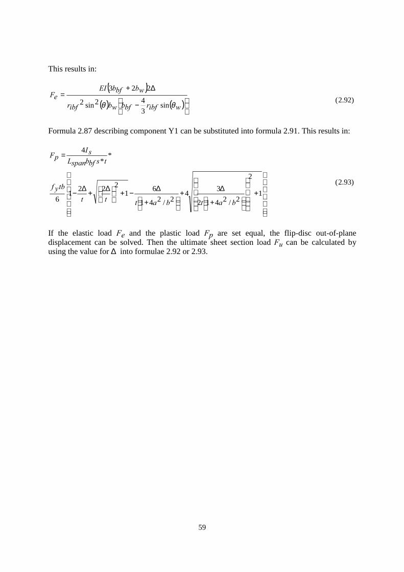
59
This results in:
( )( ) ( )
−
∆+=
wibfrbfbwbibfr
wbbfbEIeF
θθ sin342sin2
223(2.92)
Formula 2.87 describing component Y1 can be substituted into formula 2.91. This results in:
1
2
2/2412
342/241
612221
6
**
4
+
+
∆+
+
∆−+
∆+∆−
=
batbattt
tbyf
tsbfbspanLsI
pF
(2.93)
If the elastic load Fe and the plastic load Fp are set equal, the flip-disc out-of-planedisplacement can be solved. Then the ultimate sheet section load Fu can be calculated byusing the value for ∆ into formulae 2.92 or 2.93.
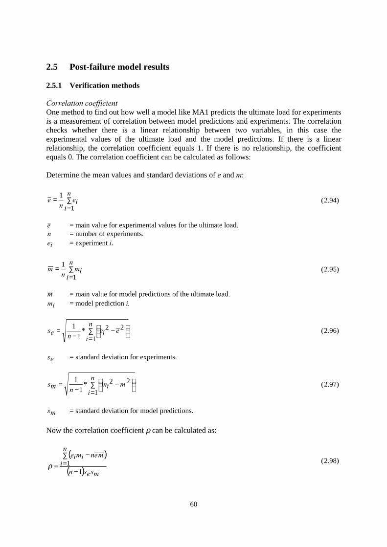
60
2.5 Post-failure model results
2.5.1 Verification methods
Correlation coefficientOne method to find out how well a model like MA1 predicts the ultimate load for experimentsis a measurement of correlation between model predictions and experiments. The correlationchecks whether there is a linear relationship between two variables, in this case theexperimental values of the ultimate load and the model predictions. If there is a linearrelationship, the correlation coefficient equals 1. If there is no relationship, the coefficientequals 0. The correlation coefficient can be calculated as follows:
Determine the mean values and standard deviations of e and m:
∑=
=n
iie
ne
1
1(2.94)
e = main value for experimental values for the ultimate load.n = number of experiments.ie = experiment i.
∑=
=n
iim
nm
1
1(2.95)
m = main value for model predictions of the ultimate load.im = model prediction i.
∑=
−−
=n
ieie
nes1
22*1
1 (2.96)
es = standard deviation for experiments.
∑=
−−
=n
imim
nms1
22*1
1 (2.97)
ms = standard deviation for model predictions.
Now the correlation coefficient ρ can be calculated as:
( )
( ) msesn
n
imenimie
11
−
∑=
−=ρ
(2.98)
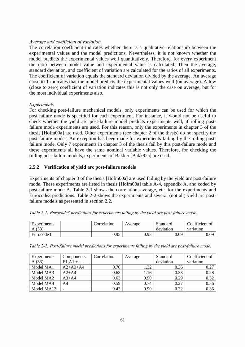
61
Average and coefficient of variationThe correlation coefficient indicates whether there is a qualitative relationship between theexperimental values and the model predictions. Nevertheless, it is not known whether themodel predicts the experimental values well quantitatively. Therefore, for every experimentthe ratio between model value and experimental value is calculated. Then the average,standard deviation, and coefficient of variation are calculated for the ratios of all experiments.The coefficient of variation equals the standard deviation divided by the average. An averageclose to 1 indicates that the model predicts the experimental values well (on average). A low(close to zero) coefficient of variation indicates this is not only the case on average, but forthe most individual experiments also.
ExperimentsFor checking post-failure mechanical models, only experiments can be used for which thepost-failure mode is specified for each experiment. For instance, it would not be useful tocheck whether the yield arc post-failure model predicts experiments well, if rolling post-failure mode experiments are used. For this reason, only the experiments in chapter 3 of thethesis [Hofm00a] are used. Other experiments (see chapter 2 of the thesis) do not specify thepost-failure modes. An exception has been made for experiments failing by the rolling post-failure mode. Only 7 experiments in chapter 3 of the thesis fail by this post-failure mode andthese experiments all have the same nominal variable values. Therefore, for checking therolling post-failure models, experiments of Bakker [Bakk92a] are used.
2.5.2 Verification of yield arc post-failure models
Experiments of chapter 3 of the thesis [Hofm00a] are used failing by the yield arc post-failuremode. These experiments are listed in thesis [Hofm00a] table A-4, appendix A, and coded bypost-failure mode A. Table 2-1 shows the correlation, average, etc. for the experiments andEurocode3 predictions. Table 2-2 shows the experiments and several (not all) yield arc post-failure models as presented in section 2.2.
Table 2-1. Eurocode3 predictions for experiments failing by the yield arc post-failure mode.
ExperimentsA (33)
Correlation Average Standarddeviation
Coefficient ofvariation
Eurocode3 0.95 0.93 0.09 0.09
Table 2-2. Post-failure model predictions for experiments failing by the yield arc post-failure mode.
ExperimentsA (33)
ComponentsE1,A1 + ....
Correlation Average Standarddeviation
Coefficient ofvariation
Model MA1 A2+A3+A4 0.70 1.32 0.36 0.27Model MA3 A2+A4 0.68 1.16 0.33 0.28Model MA2 A3+A4 0.63 0.90 0.29 0.32Model MA4 A4 0.59 0.74 0.27 0.36Model MA12 - 0.43 0.90 0.32 0.36
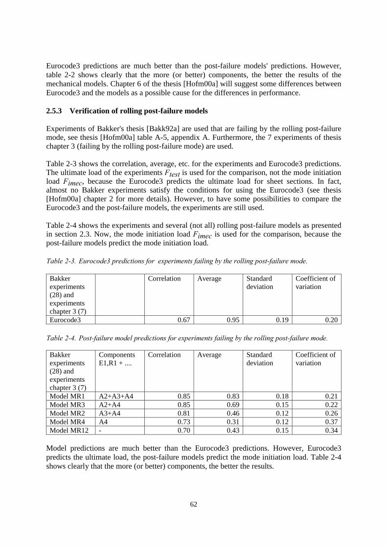
62
Eurocode3 predictions are much better than the post-failure models' predictions. However,table 2-2 shows clearly that the more (or better) components, the better the results of themechanical models. Chapter 6 of the thesis [Hofm00a] will suggest some differences betweenEurocode3 and the models as a possible cause for the differences in performance.
2.5.3 Verification of rolling post-failure models
Experiments of Bakker's thesis [Bakk92a] are used that are failing by the rolling post-failuremode, see thesis [Hofm00a] table A-5, appendix A. Furthermore, the 7 experiments of thesischapter 3 (failing by the rolling post-failure mode) are used.
Table 2-3 shows the correlation, average, etc. for the experiments and Eurocode3 predictions.The ultimate load of the experiments Ftest is used for the comparison, not the mode initiationload Fimec, because the Eurocode3 predicts the ultimate load for sheet sections. In fact,almost no Bakker experiments satisfy the conditions for using the Eurocode3 (see thesis[Hofm00a] chapter 2 for more details). However, to have some possibilities to compare theEurocode3 and the post-failure models, the experiments are still used.
Table 2-4 shows the experiments and several (not all) rolling post-failure models as presentedin section 2.3. Now, the mode initiation load Fimec is used for the comparison, because thepost-failure models predict the mode initiation load.
Table 2-3. Eurocode3 predictions for experiments failing by the rolling post-failure mode.
Bakkerexperiments(28) andexperimentschapter 3 (7)
Correlation Average Standarddeviation
Coefficient ofvariation
Eurocode3 0.67 0.95 0.19 0.20
Table 2-4. Post-failure model predictions for experiments failing by the rolling post-failure mode.
Bakkerexperiments(28) andexperimentschapter 3 (7)
ComponentsE1,R1 + ....
Correlation Average Standarddeviation
Coefficient ofvariation
Model MR1 A2+A3+A4 0.85 0.83 0.18 0.21Model MR3 A2+A4 0.85 0.69 0.15 0.22Model MR2 A3+A4 0.81 0.46 0.12 0.26Model MR4 A4 0.73 0.31 0.12 0.37Model MR12 - 0.70 0.43 0.15 0.34
Model predictions are much better than the Eurocode3 predictions. However, Eurocode3predicts the ultimate load, the post-failure models predict the mode initiation load. Table 2-4shows clearly that the more (or better) components, the better the results.
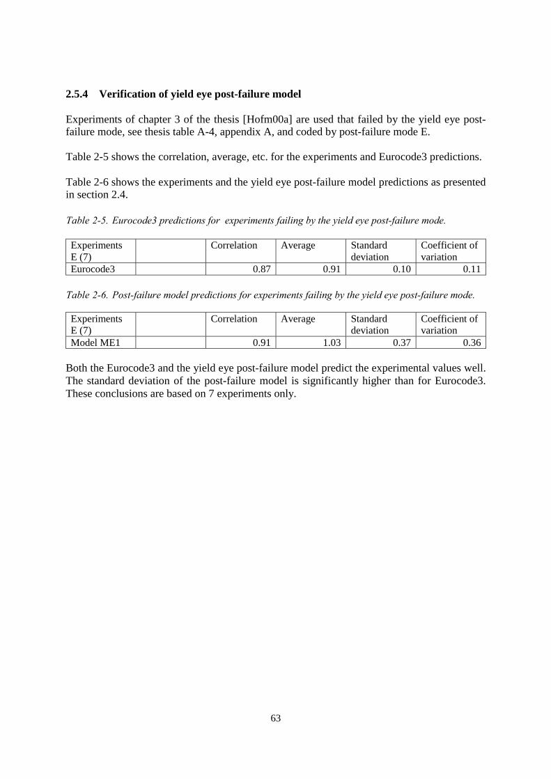
63
2.5.4 Verification of yield eye post-failure model
Experiments of chapter 3 of the thesis [Hofm00a] are used that failed by the yield eye post-failure mode, see thesis table A-4, appendix A, and coded by post-failure mode E.
Table 2-5 shows the correlation, average, etc. for the experiments and Eurocode3 predictions.
Table 2-6 shows the experiments and the yield eye post-failure model predictions as presentedin section 2.4.
Table 2-5. Eurocode3 predictions for experiments failing by the yield eye post-failure mode.
ExperimentsE (7)
Correlation Average Standarddeviation
Coefficient ofvariation
Eurocode3 0.87 0.91 0.10 0.11
Table 2-6. Post-failure model predictions for experiments failing by the yield eye post-failure mode.
ExperimentsE (7)
Correlation Average Standarddeviation
Coefficient ofvariation
Model ME1 0.91 1.03 0.37 0.36
Both the Eurocode3 and the yield eye post-failure model predict the experimental values well.The standard deviation of the post-failure model is significantly higher than for Eurocode3.These conclusions are based on 7 experiments only.
64
2.6 Conclusions
A methodology to develop post-failure mechanical models has been presented. Thismethodology separates sheet section behaviour into components.
For the yield arc and rolling post-failure modes, mechanical models have been developedwhich first predict the ultimate load for a piece of the sheet section above the load-bearingplate. Hereafter, this prediction is corrected for pieces of the sheet section adjacent to theload-bearing plate and the length effect. Mathematical techniques have been used to simplifythe model equations.
For the yield eye post-failure model the model transforms elastic cross-section behaviour inan elastic flip-disc out-of-plane displacement. For plastic flip-disc behaviour, an existingmodel is used. By setting equal elastic and plastic loads of the section, the ultimate load canbe predicted.
The developed models are compared with experiments. For the yield arc and yield eye post-failure modes the experiments presented in chapter 3 of thesis [Hofm00a] are used. For therolling post-failure mode, experiments carried out by Bakker are used. The more detailed themodels are, the higher is the correlation with the experiments. This indicates that themethodology works well. The components used in this report are exemplary. Bettercomponents may result in a better correlation.
65
3 Appendix detailed derivations post-failure models
3.1 Derivation of formulae 2.18 to 2.21
These formulae were derived by Maarten Vaessen in 1995 [Vaes95a]. Some remarks shouldbe made to fully understand his master thesis in the context of this thesis.
Page 125 [Vaes95a]: ‘… of the establishment of the portal frame model both…'The ‘portal frame model’ as mentioned by Vaessen was intended to describe the elastic webcrippling stiffness of hat sections, sheet sections, and trapezoidal sheeting. The first step inorder to create this ‘portal frame model’ was to predict the relation between the applied forcesand the indentation of a small prismatic cross-section part of a sheet section. This smallprismatic part can be seen as the same as the ‘modelled cross-section’ in this thesis. However,Vaessen assumes a cross-section dx small. In this thesis, the modelled cross-section has awidth equal to Llb.
Page 125: ‘… the assumptions as stated in section 3.2, the cross section…'Two of the assumptions as stated in section 3.2 are related to the ‘portal frame model’ and arenot important for the modelled cross-section in this thesis. Important assumptions are: Therounding of the corners of the modelled cross-section is ignored (1). However, theeccentricity of the two concentrated loads due to the rounding is taken into account. Althoughthe support creates an equally distributed load at the top flange first, curling of the top flangemakes it acceptable to replace the distributed load by two concentrated loads (2). Sheardeformations in the modelled cross-section are ignored (3). Only axial forces and bendingmoments are taken into account.
Page 125: Figure A.1Vaessen rotates the modelled cross-section 180 degrees in all his figures. Vaessen defines thebottom flange in this report as top flange and vice versa.
Page 130: ‘… the reciprocal two-dimensional web crippling…'This reciprocal two-dimensional web crippling stiffness equals the web crippling deformationdivided by the support load. Therefore, the support load equals the web crippling stiffnessdivided by this reciprocal web crippling stiffness. Rewriting the formulae in the master thesisand defining variables as used in this report, formula 2.18 to 2.21 can be derived.
Page 125-130: defining variablesThe following variables are used in Vaessen's thesis:
btf = top flange width.ri;tf = interior corner radius between web and top flange.θw = angle between web and flange.F = distributed load of support, modelled as concentrated load.Rh = horizontal reaction.A,B,C,D = points.ui = horizontal displacement point i.wi = vertical displacement point i.
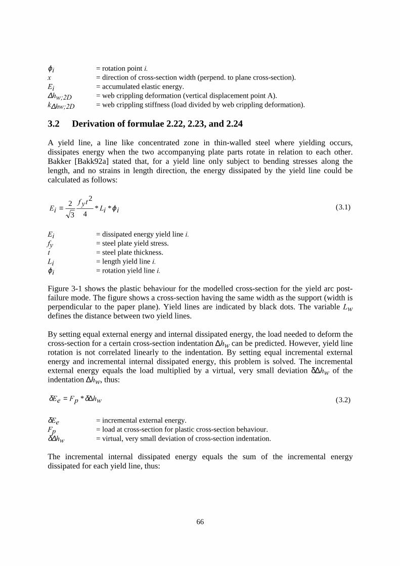
66
ϕi = rotation point i.x = direction of cross-section width (perpend. to plane cross-section).Ei = accumulated elastic energy.∆hw;2D = web crippling deformation (vertical displacement point A).k∆hw;2D = web crippling stiffness (load divided by web crippling deformation).
3.2 Derivation of formulae 2.22, 2.23, and 2.24
A yield line, a line like concentrated zone in thin-walled steel where yielding occurs,dissipates energy when the two accompanying plate parts rotate in relation to each other.Bakker [Bakk92a] stated that, for a yield line only subject to bending stresses along thelength, and no strains in length direction, the energy dissipated by the yield line could becalculated as follows:
iiLtyf
iE ϕ**4
2
32= (3.1)
Ei = dissipated energy yield line i.fy = steel plate yield stress.t = steel plate thickness.Li = length yield line i.ϕi = rotation yield line i.
Figure 3-1 shows the plastic behaviour for the modelled cross-section for the yield arc post-failure mode. The figure shows a cross-section having the same width as the support (width isperpendicular to the paper plane). Yield lines are indicated by black dots. The variable Lwdefines the distance between two yield lines.
By setting equal external energy and internal dissipated energy, the load needed to deform thecross-section for a certain cross-section indentation ∆hw can be predicted. However, yield linerotation is not correlated linearly to the indentation. By setting equal incremental externalenergy and incremental internal dissipated energy, this problem is solved. The incrementalexternal energy equals the load multiplied by a virtual, very small deviation δ∆hw of theindentation ∆hw, thus:
whpFeE ∆= δδ * (3.2)
δEe = incremental external energy.Fp = load at cross-section for plastic cross-section behaviour.δ∆hw = virtual, very small deviation of cross-section indentation.
The incremental internal dissipated energy equals the sum of the incremental energydissipated for each yield line, thus:
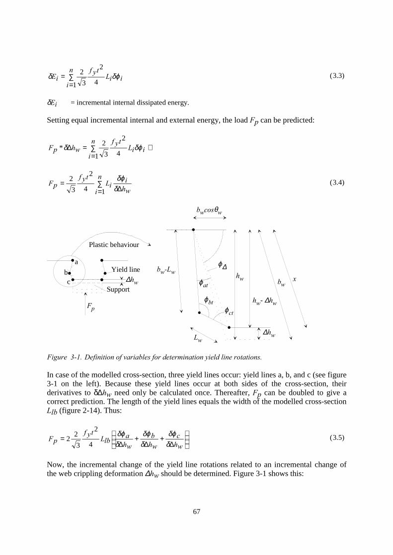
67
∑=
=n
iiiL
tyfiE
1 4
2
32 δϕδ (3.3)
δEi = incremental internal dissipated energy.
Setting equal incremental internal and external energy, the load Fp can be predicted:
⇔∑=
=∆n
iiiL
tyfwhpF
1 4
2
32* δϕδ
∑= ∆
=n
i whi
iLtyf
pF14
2
32
δδϕ (3.4)
Support
Plastic behaviour
Yield line
hw- ∆hw
∆hw
bwxhw
Lw
bw-Lw
bwcosθw
ϕat
ϕbtϕct
ϕ∆
Fp
∆hw
abc
Figure 3-1. Definition of variables for determination yield line rotations.
In case of the modelled cross-section, three yield lines occur: yield lines a, b, and c (see figure3-1 on the left). Because these yield lines occur at both sides of the cross-section, theirderivatives to δ∆hw need only be calculated once. Thereafter, Fp can be doubled to give acorrect prediction. The length of the yield lines equals the width of the modelled cross-sectionLlb (figure 2-14). Thus:
∆
+∆
+∆
=whc
whb
wha
lbLtyf
pFδδϕ
δδϕ
δδϕ
4
2
322 (3.5)
Now, the incremental change of the yield line rotations related to an incremental change ofthe web crippling deformation ∆hw should be determined. Figure 3-1 shows this:
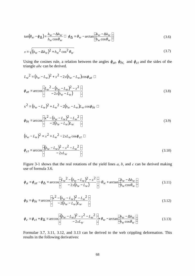
68
( )
∆−−=∆⇔
∆−=∆−
wwbwhwh
wwwbwhwh
w θθϕ
θϕθ
cosarctan
costan (3.6)
( ) wwbwhwhx θ2cos22 +∆−= (3.7)
Using the cosines rule, a relation between the angles ϕat, ϕbt, and ϕct and the sides of thetriangle abc can be derived.
( ) ( ) ⇔−−+−= atwLwbxxwLwbwL ϕcos2222
( )( )
−−−−−
=wLwbx
xwLwbwLat 2
222arccosϕ (3.8)
( ) ( ) ⇔−−+−= btwLwLwbwLwLwb ϕcos2222x
( )( )
−−−−−
=wLwLwb
wLwLwbbt 2
222xarccosϕ (3.9)
( ) ⇔−+=− ctwxLwLxwLwb ϕcos2222
( )
−−−−
=wxL
wLxwLwbct 2
222arccosϕ (3.10)
Figure 3-1 shows that the real rotations of the yield lines a, b, and c can be derived makinguse of formula 3.6.
( )( )
∆−+−
−−−−−
=∆−=wwbwhwh
wwLwbx
xwLwbwLata θ
θϕϕϕcos
arctan2
222arccos (3.11)
( )( )
−−−−−
==wLwLwb
wLwLwbbtb 2
222xarccos ϕϕ (3.12)
( )
∆−−+
−−−−
=∆+=wwbwhwh
wwxL
wLxwLwbctc θ
θϕϕϕcos
arctan2
222arccos (3.13)
Formulae 3.7, 3.11, 3.12, and 3.13 can be derived to the web crippling deformation. Thisresults in the following derivatives:
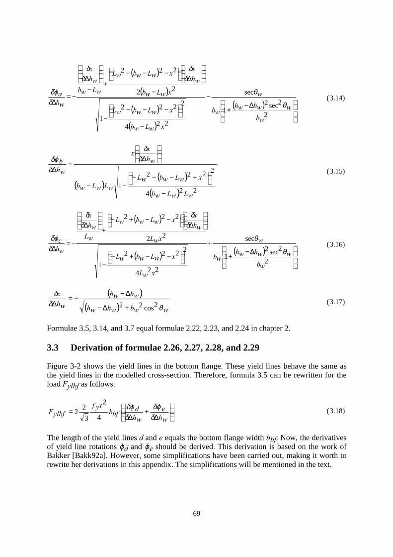
69
( )
( )
( )
( )
( )
∆−+
−
−
−−−−
−
∆
−−−+
−
∆
−=∆
2
2sec21
sec
224
22221
22
222
wbwwhwh
wb
w
xwLwb
xwLwbwL
xwLwbwh
xxwLwbwL
wLwbwh
x
wha
θ
θ
δδ
δδ
δδϕ
(3.14)
( )( )
( ) 224
22221
wLwLwb
xwLwbwLwLwLwb
whxx
whb
−
+−−−−−
∆
=∆
δδ
δδϕ
(3.15)
( )
( ) ( )
∆−+
+
−−+−−
∆
−−+−+
∆
−=∆
2
2sec21
sec
224
22221
22
222
wbwwhwh
wb
w
xwL
xwLwbwL
xwLwh
xxwLwbwL
wLwh
x
whc
θ
θ
δδ
δδ
δδϕ
(3.16)
( )( ) wwbwhwh
whwh
whx
θδδ
2cos22 +∆−
∆−−=
∆ (3.17)
Formulae 3.5, 3.14, and 3.7 equal formulae 2.22, 2.23, and 2.24 in chapter 2.
3.3 Derivation of formulae 2.26, 2.27, 2.28, and 2.29
Figure 3-2 shows the yield lines in the bottom flange. These yield lines behave the same asthe yield lines in the modelled cross-section. Therefore, formula 3.5 can be rewritten for theload Fylbf as follows.
∆
+∆
=whe
whd
bfbtyf
ylbfFδδϕ
δδϕ
4
2
322 (3.18)
The length of the yield lines d and e equals the bottom flange width bbf. Now, the derivativesof yield line rotations ϕd and ϕe should be derived. This derivation is based on the work ofBakker [Bakk92a]. However, some simplifications have been carried out, making it worth torewrite her derivations in this appendix. The simplifications will be mentioned in the text.
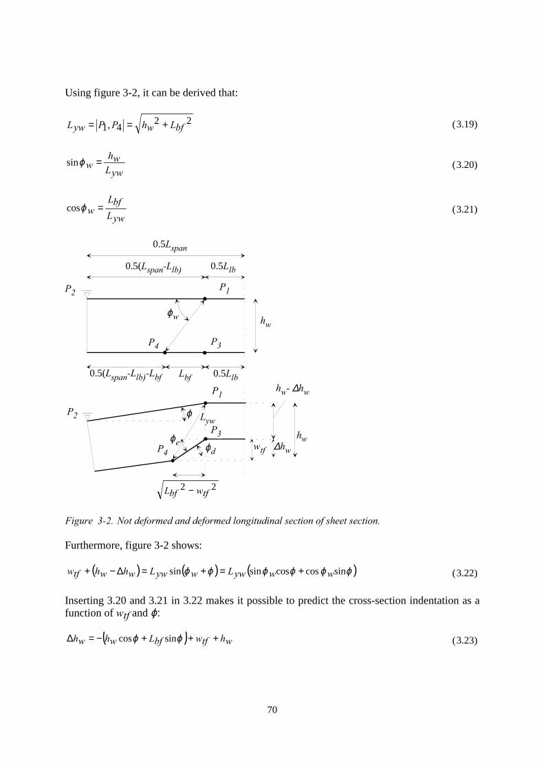
70
Using figure 3-2, it can be derived that:
224,1 bfLwhPPywL +== (3.19)
ywLwh
w =ϕsin (3.20)
ywLbfL
w =ϕcos (3.21)
22 tfwbfL −
0.5Lspan
0.5(Lspan-Llb) 0.5Llb
P2 P1
hwϕw
P3P4
0.5(Lspan-Llb)-Lbf Lbf 0.5Llb
P2
P1
P4
P3
ϕ
ϕe ϕd
Lyw
wtf
hw- ∆hw
hw∆hw
Figure 3-2. Not deformed and deformed longitudinal section of sheet section.
Furthermore, figure 3-2 shows:
( ) ( ) ( )ϕϕϕϕϕϕ sin coscossinsin wwywLwywLwhwhtfw +=+=∆−+ (3.22)
Inserting 3.20 and 3.21 in 3.22 makes it possible to predict the cross-section indentation as afunction of wtf and ϕ:
( ) whtfwbfLwhwh +++−=∆ ϕϕ sincos (3.23)
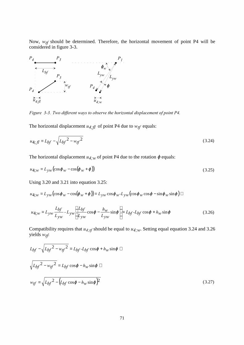
71
Now, wtf should be determined. Therefore, the horizontal movement of point P4 will beconsidered in figure 3-3.
P4 P3 P1
P4P4
P3
Lbf
u4;fl
wtf
u4;w
Lyw Lyw
ϕ
ϕw
Figure 3-3. Two different ways to observe the horizontal displacement of point P4.
The horizontal displacement u4;fl of point P4 due to wtf equals:
22;4 tfwbfLbfLflu −−= (3.24)
The horizontal displacement u4;w of point P4 due to the rotation ϕ equals:
( )( )ϕϕϕ +−= wwywLwu coscos;4 (3.25)
Using 3.20 and 3.21 into equation 3.25:
( )( ) ( )⇔−=+−= ϕϕϕϕϕϕϕϕ sinsincoscoscoscoscos;4 wwyw-LwywLwwywLwu
ϕϕϕϕ sincossincos-;4 whbf-LbfLywLwh
ywLbfL
ywLywLbfL
ywLwu +=
−= (3.26)
Compatibility requires that u4;tf should be equal to u4;w. Setting equal equation 3.24 and 3.26yields wtf:
⇔+=−− ϕϕ sincos22whbf-LbfLtfwbfLbfL
⇔−=− ϕϕ sincos22whbfLtfwbfL
( )2sincos2 ϕϕ whbfLbfLtfw −−= (3.27)
72
Inserting equation 3.27 into equation 3.23 describes the relationship between the webcrippling deformation ∆hw and the rotation ϕ :
( ) ( ) whwhbfLbfLbfLwhwh +−−++−=∆ 2sincos2sincos ϕϕϕϕ (3.28)
This equation can be differentiated with respect to ϕ as follows:
( ) ( )( )( )2sincos2
cossinsincoscossin
ϕϕ
ϕϕϕϕϕϕ
δϕδ
whbfLbfL
whbfLwhbfLbfLwhwh
−−
+−+−=∆
(3.29)
Rewriting equations 3.23 and 3.27, it can be concluded that:
( ) ( ) whtfwwhbfLwhwhtfwbfLwhwh ∆−+=+⇔+++−=∆ ϕϕϕϕ sincossincos (3.30)
( ) ( ) 22sincos2sincos2tfwbfLwhbfLwhbfLbfLtfw −=−⇔−−= ϕϕϕϕ (3.31)
Substituting 3.30 and 3.31 into 3.29 yields:
( ) ( )tfw
whwhtfwbfL
tfwwhtfwwhtfwbfL
tfwbfLwh ∆−−=
∆−+−+−−=
∆22
22
22δϕ
δ (3.32)
Now, the incremental change of ϕ for an incremental change of ∆hw can be determined asfollows:
( )whwhtfwbfL
tfw
wh ∆−−=
∆ 22δδϕ
(3.33)
The variable wtf can be predicted using 3.27. The variable ϕ in 3.27 can be determined byiterative solving 3.28. Figure 3-2 shows:
bfLtfw
e arcsin=ϕ (3.34)
This equation 3.34 can be differentiated with respect to ∆hw, yielding:
cos1
whtfw
ebfLwhe
∆=
∆ δδ
ϕδδϕ
(3.35)
Figure 3-2 shows:
73
22
cosbfL
tfwbfLe
−=ϕ (3.36)
Furthermore:
( )( )( )whwhtfwbfL
tfw
tfwwhbfLwhbfL
whtfw
whtfw
∆−−
+−=
∆=
∆ 22
cossinsincos ϕϕϕϕδδϕ
δϕδ
δδ
(3.37)
Using 3.30 and 3.31, equation 3.37 can be rewritten as:
( )( )
⇔∆−−
∆−+−=
∆=
∆whwhtfwbfL
tfw
tfwwhtfwwhtfwbfL
whtfw
whtfw
22
22
δδϕ
δϕδ
δδ
( )( )whwh
whtfwwh
whtfw
∆−
∆−+=
∆δδ
(3.38)
Now, using equation 3.36 and 3.37, formula 3.35 yields:
( )( )
22
tfwbfLwhwh
whtfwwh
whe
−∆−
∆−+=
∆δδϕ
(3.39)
From figure 3-2 it can also be seen that:
-whwh
ewhded ∆∆
=∆
⇔−=δ
δϕδδϕ
δδϕϕϕϕ (3.40)
In this appendix, formulae 2.26, 2.27, 2.28, and 2.29 have been derived as equation 3.18,3.39, 3.27 and 3.40.
3.4 Derivation of formulae 2.69, 2.70, 2.71, 2.72, and 2.73
These formulae predict the plastic behaviour of the rolling post-failure mode, for the modelledcross-section (figure 2-17). Figure 2-19 in appendix 2 shows the rolling post-failure mode,however, in this appendix 3 more detailed drawings will be used. Figure 3-4 shows the rollingpost-failure mode for the modelled cross-section.
Although the derivations of these formulae can be red in the Bakker's thesis [Bakk92a], theywill be copied here for convenience.
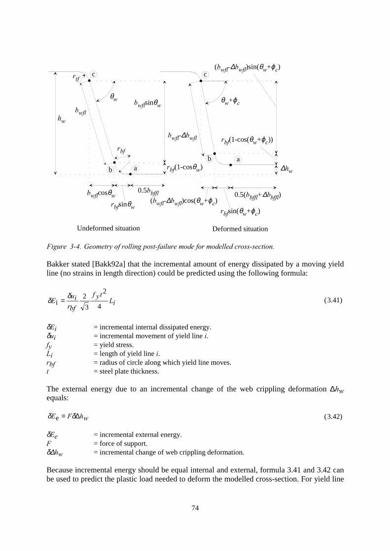
74
ab
c
ab
c
Undeformed situation Deformed situation
rtf
bwflhw
θw
rbf
bwflsinθw
bwfl-∆bwfl
bwflcosθwrbfsinθw
0.5bbffl
rbf(1-cosθw)
(bwfl-∆bwfl)cos(θw+ϕc)rbfsin(θw+ϕc)
0.5(bbffl+∆bbffl)
∆hw
rbf(1-cos(θw+ϕc))
(bwfl-∆bwfl)sin(θw+ϕc)
θw+ϕc
Figure 3-4. Geometry of rolling post-failure mode for modelled cross-section.
Bakker stated [Bakk92a] that the incremental amount of energy dissipated by a moving yieldline (no strains in length direction) could be predicted using the following formula:
iLtyf
bfriuE
4
2
32
iδ
δ = (3.41)
δEi = incremental internal dissipated energy.δui = incremental movement of yield line i.fy = yield stress.Li = length of yield line i.rbf = radius of circle along which yield line moves.t = steel plate thickness.
The external energy due to an incremental change of the web crippling deformation ∆hwequals:
whFE ∆= δδ e (3.42)
δEe = incremental external energy.F = force of support.δ∆hw = incremental change of web crippling deformation.
Because incremental energy should be equal internal and external, formula 3.41 and 3.42 canbe used to predict the plastic load needed to deform the modelled cross-section. For yield line
75
"c" in figure 3-4, which is a normal fixed yield line (this yield line rotates only), formula 3.3is used.
⇔=∆ iLtyf
bfriu
whF4
2
32δ
δ
lbLtyf
whc
lbLtyf
bfrwhbu
lbLtyf
bfrwhau
F4
2
322
4
2
3212
4
2
3212
∆+
∆+
∆=
δδϕ
δδ
δδ (3.43)
Formula 3.43 equals formula 2.69. Now, the incremental movements of yield lines "a" and"b" should be determined as a result of an incremental change of the web cripplingdeformation ∆hw. First, the flat widths of several cross-section variables are determined, seefigure 3-4 for their definition. The variables bbf and bw are the widths of the bottom flangeand the web measured between the points of intersection of the web and flange midlines.
−=
2tan2 wbfrbfbbfflb θ
(3.44)
( )
+−=
2tan wbfrtfrwbwflb θ
(3.45)
Due to the rolling post-failure mode, the flat width of the bottom flange increases from bbffl to(bbffl+∆bbffl), the flat width of the web decreases from bwfl to (bwfl-∆bwfl). The yield linedisplacements u1 and u2 can then be determined as:
bfflΔbau21= (3.46)
wflbbu ∆= (3.47)
The formulae describing the incremental yield line deformations due to an incremental webcrippling deformation δ∆hw can best be derived as follows. First by determining theincremental yield line deformations due to the incremental rotation δϕc in yield line "c" at thetop of the web. Therefore the changes in the flat widths of the elements must be expressed asa function of the rotation ϕc. Since the total length of flange and web elements does notchange, it can be derived from figure 3-4 that:
( ) ( )⇔∆−+++∆−=++ bfflbbfflbcwbfrwflbwflbbfflbwθbfrwflb21
21 ϕθ
( )cbfrwflbbfflb ϕ−∆=∆ 2 (3.48)
76
The distance between the tops of the webs does not change either, and therefore:
( ) ( )
( ) ( )bfflbbfflbwbfr
cwwflbwflbbfflbwbfrwwflb
∆+++
++∆−=++
21
3sin
cos21sincos
ϕθ
ϕθθθ(3.49)
Combining formulae 3.48 and 3.49 results in:
( )( ) ( )( )( )cw
cwcwbfrcwwwflbwflb
ϕθϕθϕθϕθθ
+−+−+++−
=∆cos1
sinsincoscos(3.50)
The incremental changes in the flat widths of the bottom flange and the web due to theincremental rotation δϕc can be determined by deriving these widths with respect to ϕc:
−
∂
∆∂=
∂
∆∂=
∆bfr
c
wflb
c
bfflb
c
bfflbϕϕδϕ
δ(3.51)
( ) ( )( ) bfr
cwcwwflbwflb
cwflb
cwflb
++−
+∆−=
∂∆∂
=∆
ϕθϕθ
ϕδϕδ
cos1sin
(3.52)
To determine the incremental yield line displacements δua and δub due to an incremental webcrippling deformation δ∆hw, this deformation must be determined as a function of theincremental rotation δϕc. Therefore the web crippling deformation ∆hw must be expressed asa function of the rotation ϕc.
From figure 3-4 it can be seen that:
( ) ( ) ( )( )wcwbfrcwwflbwflbwwflbwh θϕθϕθθ coscossinsin −+++∆−−=∆ (3.53)
Hence:
( ) ( ) ( ) ( )cwbfrcwwflbwflbcwcwflb
cwh ϕθϕθϕθ
δϕδ
δϕδ +−+∆−−+
∆=∆ sincossin (3.54)
Inserting formula 3.52 into 3.54 results in:
wflbwflbcwh ∆−=
∆δϕ
δ(3.55)
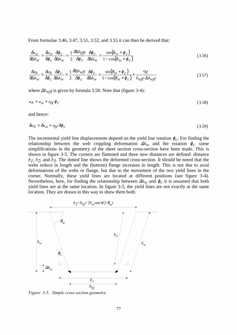
77
From formulae 3.46, 3.47, 3.51, 3.52, and 3.55 it can then be derived that:
( )( )cw
cwwhc
c
tfflb
whc
cau
whau
ϕθϕθ
δδϕ
δϕδ
δδϕ
δϕδ
δδ
+−+
=∆
∆=
∆=
∆ cos1sin
21 (3.56)
( )( ) wflb-wflb
bfr
cwcw
whc
cwflb
whc
cbu
whbu
∆+
+−+=
∆
∆=
∆=
∆ ϕθϕθ
δδϕ
δϕδ
δδϕ
δϕδ
δδ
cos1sin
21
(3.57)
where ∆bwfl is given by formula 3.50. Note that (figure 3-4):
cbfraubu ϕ+= (3.58)
and hence:
cbfraubu δϕδδ += (3.59)
The incremental yield line displacements depend on the yield line rotation ϕc. For finding therelationship between the web crippling deformation ∆hw and the rotation ϕc somesimplifications in the geometry of the sheet section cross-section have been made. This isshown in figure 3-5. The corners are flattened and three new distances are defined: distanceb1, b2, and b3. The dotted line shows the deformed cross-section. It should be noted that thewebs reduce in length and the (bottom) flange increases in length. This is not due to axialdeformations of the webs or flange, but due to the movement of the two yield lines in thecorner. Normally, these yield lines are located at different positions (see figure 3-4).Nevertheless, here, for finding the relationship between ∆hw and ϕc it is assumed that bothyield lines are at the same location. In figure 3-5, the yield lines are not exactly at the samelocation. They are drawn in this way to show them both.
bbf
b1
bw
b2
θw
ϕc
hw
∆hw
b3=bbf+2bwsin(π/2-θw)
Figure 3-5. Simple cross-section geometry.
78
Using figure 3-5 it can be shown that:
−−−=∆ cwbwhwh ϕθπ
2cos2 (3.60)
The distance between the tops of the webs b3 is assumed to remain equal. For sheet sectionsand sheeting, this is true. If the distance remains equal then:
( )2
135.02
sinb
bbcw
−=
−− ϕθπ
(3.61)
The total length of the two webs and bottom flange cannot change:
2212 bbwbbfb +=+ (3.62)
Formula 3.62 can be solved for b1 that can be substituted in formula 3.61. Note that c1 is anew substitution variable used.
211
221
2
25.035.0
2sin
bc
bbc
bbwbbfbb
cw +=+
=+−−
=
−− ϕθπ (3.63)
Formula 3.63 can be used to solve b2 that can be inserted into formula 3.60:
12
sin
2cos1
−
−−
−−
−=∆cw
cwcwhwh
ϕθπ
ϕθπ
(3.64)
With c1 and b3 defined in formula 3.63 and figure 3-5 respectively. If it is assumed that angleϕc is small, the following parts of formula 3.64 can be rewritten as follows:
cwcw
cw
ϕθπϕθπ
ϕθπ
sin2
sincos2
cos
2cos
−+
−
=
−−
(3.65)
−−
−=
−−
−
=
−−
wcwcwcw
cw
θπϕθπϕθπϕθπ
ϕθπ
2cos
2sinsin
2coscos
2sin
2sin
(3.66)
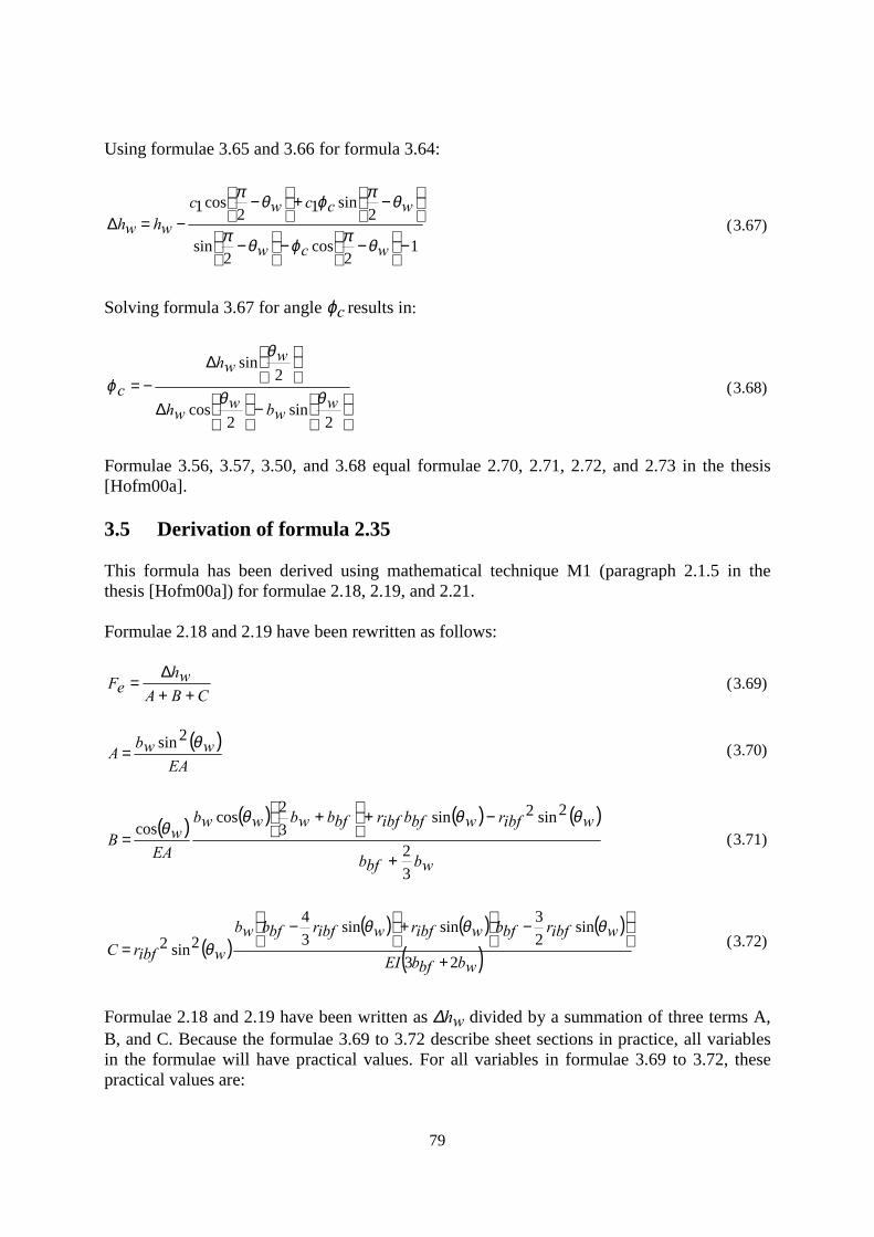
79
Using formulae 3.65 and 3.66 for formula 3.64:
12
cos2
sin
2sin12
cos1
−
−−
−
−+
−
−=∆wcw
wccwcwhwh
θπϕθπ
θπϕθπ
(3.67)
Solving formula 3.67 for angle ϕc results in:
−
∆
∆
−=
2sin
2cos
2sin
wwbw
wh
wwh
c θθ
θ
ϕ (3.68)
Formulae 3.56, 3.57, 3.50, and 3.68 equal formulae 2.70, 2.71, 2.72, and 2.73 in the thesis[Hofm00a].
3.5 Derivation of formula 2.35
This formula has been derived using mathematical technique M1 (paragraph 2.1.5 in thethesis [Hofm00a]) for formulae 2.18, 2.19, and 2.21.
Formulae 2.18 and 2.19 have been rewritten as follows:
CBA
wheF
++∆
= (3.69)
( )
2sinEA
wwbA
θ= (3.70)
( ) ( ) ( ) ( )
wbbfb
wibfrwbfbibfrbfbwbwwb
EAwB
32
2sin2sin32cos
cos
+
−+
+
=θθθ
θ (3.71)
( )( ) ( ) ( )
( )wbbfbEI
wibfrbfbwibfrwibfrbfbwb
wibfrC23
sin23sinsin
34
2sin2+
−+
−
=θθθ
θ (3.72)
Formulae 2.18 and 2.19 have been written as ∆hw divided by a summation of three terms A,B, and C. Because the formulae 3.69 to 3.72 describe sheet sections in practice, all variablesin the formulae will have practical values. For all variables in formulae 3.69 to 3.72, thesepractical values are:
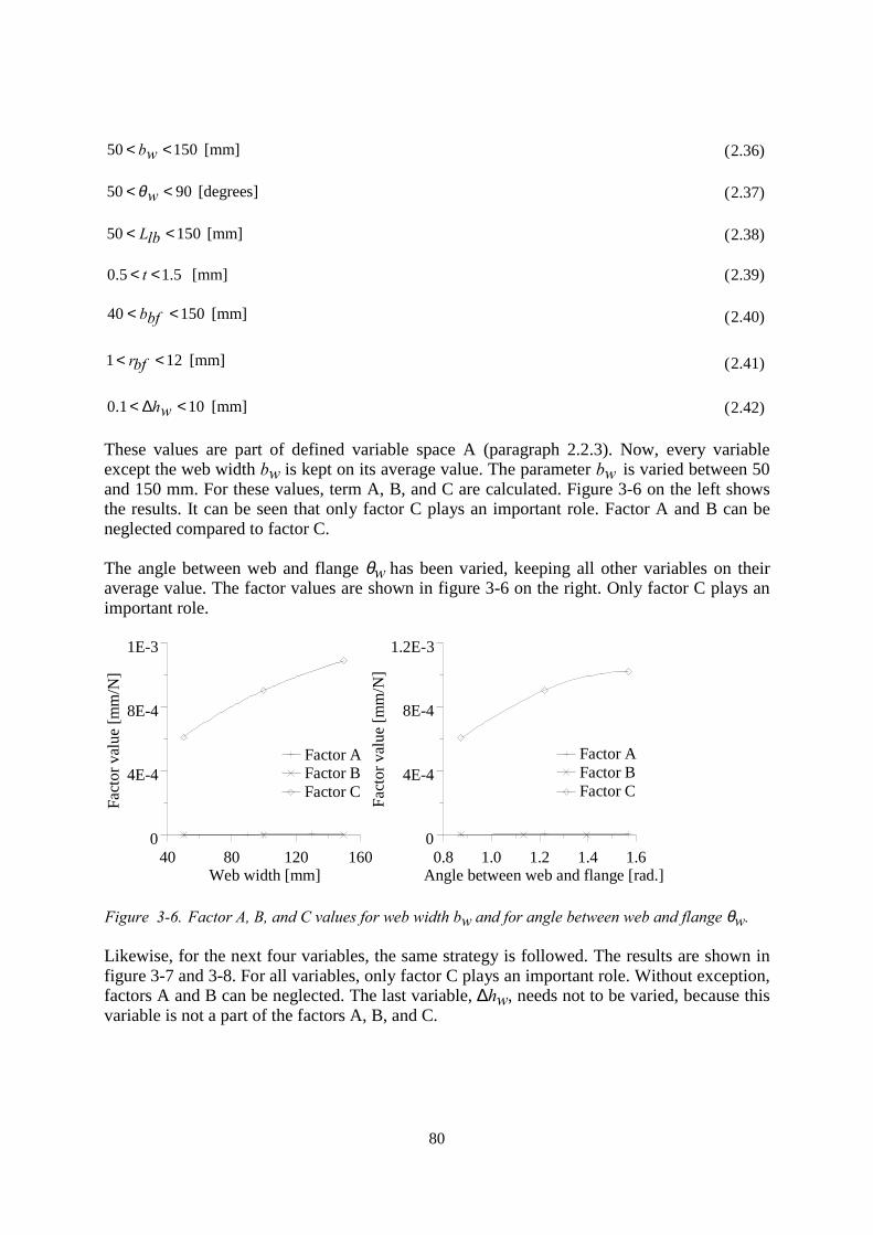
80
15050 << wb [mm] (2.36)
9050 << wθ [degrees] (2.37)
15050 << lbL [mm] (2.38)
5.15.0 << t [mm] (2.39)
15040 << bfb [mm] (2.40)
121 << bfr [mm] (2.41)
101.0 <∆< wh [mm] (2.42)
These values are part of defined variable space A (paragraph 2.2.3). Now, every variableexcept the web width bw is kept on its average value. The parameter bw is varied between 50and 150 mm. For these values, term A, B, and C are calculated. Figure 3-6 on the left showsthe results. It can be seen that only factor C plays an important role. Factor A and B can beneglected compared to factor C.
The angle between web and flange θw has been varied, keeping all other variables on theiraverage value. The factor values are shown in figure 3-6 on the right. Only factor C plays animportant role.
40 80 120 160Web width [mm]
0
4E-4
8E-4
1E-3
Fact
or v
alue
[mm
/N]
Factor AFactor BFactor C
0.8 1.0 1.2 1.4 1.6Angle between web and flange [rad.]
0
4E-4
8E-4
1.2E-3
Fact
or v
alue
[mm
/N]
Factor AFactor BFactor C
Figure 3-6. Factor A, B, and C values for web width bw and for angle between web and flange θw.
Likewise, for the next four variables, the same strategy is followed. The results are shown infigure 3-7 and 3-8. For all variables, only factor C plays an important role. Without exception,factors A and B can be neglected. The last variable, ∆hw, needs not to be varied, because thisvariable is not a part of the factors A, B, and C.
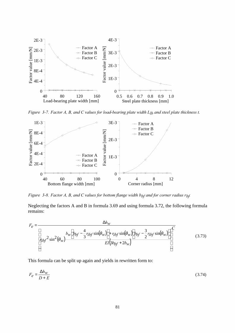
81
40 80 120 160Load-bearing plate width [mm]
0
4E-4
8E-4
1E-3
2E-3
2E-3
Fact
or v
alue
[mm
/N]
0.5 0.6 0.7 0.8 0.9 1.0Steel plate thickness [mm]
0
1E-3
2E-3
3E-3
4E-3
Fact
or v
alue
[mm
/N]Factor A
Factor BFactor C
Factor AFactor BFactor C
Figure 3-7. Factor A, B, and C values for load-bearing plate width Llb and steel plate thickness t.
0 4 8 12Corner radius [mm]
0
1E-3
2E-3
3E-3
Fact
or v
alue
[mm
/N]
40 60 80 100Bottom flange width [mm]
0
2E-4
4E-4
6E-4
8E-4
1E-3
Fact
or v
alue
[mm
/N]
Factor AFactor BFactor C
Factor AFactor BFactor C
Figure 3-8. Factor A, B, and C values for bottom flange width bbf and for corner radius rbf.
Neglecting the factors A and B in formula 3.69 and using formula 3.72, the following formularemains:
( )( ) ( ) ( )
( )
23
sin23sinsin
34
2sin2
C
wbbfbEI
wibfrbfbwibfrwibfrbfbwbwibfr
wheF
+
−+
−
∆=
θθθθ
(3.73)
This formula can be split up again and yields in rewritten form to:
EDwh
eF+
∆= (3.74)
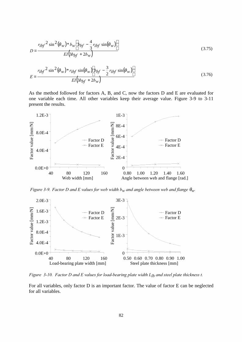
82
( ) ( )
( )wbbfbEI
wibfrbfbwbwibfrD
23
sin34*2sin2
+
−
=θθ
(3.75)
( ) ( ) ( )
( )wbbfbEI
wibfrbfbwibfrwibfrE
23
sin23sin*2sin2
+
−
=θθθ
(3.76)
As the method followed for factors A, B, and C, now the factors D and E are evaluated forone variable each time. All other variables keep their average value. Figure 3-9 to 3-11present the results.
40 80 120 160Web width [mm]
0.0E+0
4.0E-4
8.0E-4
1.2E-3
Fact
or v
alue
[mm
/N]
Factor DFactor E
0.80 1.00 1.20 1.40 1.60Angle between web and flange [rad.]
0
2E-4
4E-4
6E-4
8E-4
1E-3Fa
ctor
val
ue [m
m/N
]
Factor DFactor E
Figure 3-9. Factor D and E values for web width bw and angle between web and flange θw.
40 80 120 160Load-bearing plate width [mm]
0.0E+0
4.0E-4
8.0E-4
1.2E-3
1.6E-3
2.0E-3
0.50 0.60 0.70 0.80 0.90 1.00Steel plate thickness [mm]
0
1E-3
2E-3
3E-3
Fact
or v
alue
[mm
/N]
Fact
or v
alue
[mm
/N]
Factor DFactor E
Factor DFactor E
Figure 3-10. Factor D and E values for load-bearing plate width Llb and steel plate thickness t.
For all variables, only factor D is an important factor. The value of factor E can be neglectedfor all variables.
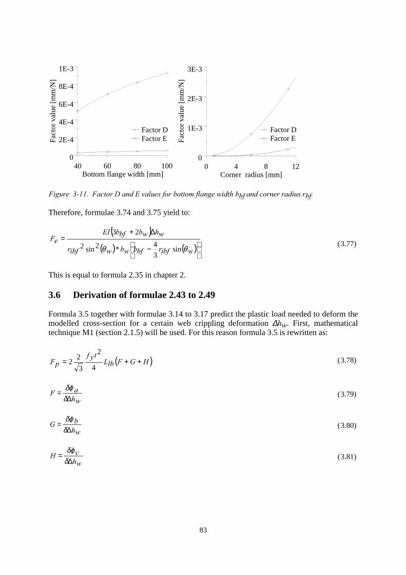
83
40 60 80 100Bottom flange width [mm]
0
2E-4
4E-4
6E-4
8E-4
1E-3
0 4 8 12Corner radius [mm]
0
1E-3
2E-3
3E-3
Fact
or v
alue
[mm
/N]
Fact
or v
alue
[mm
/N]
Factor DFactor E
Factor DFactor E
Figure 3-11. Factor D and E values for bottom flange width bbf and corner radius rbf.
Therefore, formulae 3.74 and 3.75 yield to:
( )( ) ( )
−
∆+=
wibfrbfbwbwibfr
whwbbfbEIeF
θθ sin34*2sin2
23(3.77)
This is equal to formula 2.35 in chapter 2.
3.6 Derivation of formulae 2.43 to 2.49
Formula 3.5 together with formulae 3.14 to 3.17 predict the plastic load needed to deform themodelled cross-section for a certain web crippling deformation ∆hw. First, mathematicaltechnique M1 (section 2.1.5) will be used. For this reason formula 3.5 is rewritten as:
( )HGFlbLtyf
pF ++=4
2
322 (3.78)
whaF
∆=
δδϕ
(3.79)
whbG
∆=
δδϕ
(3.80)
whcH
∆=
δδϕ
(3.81)
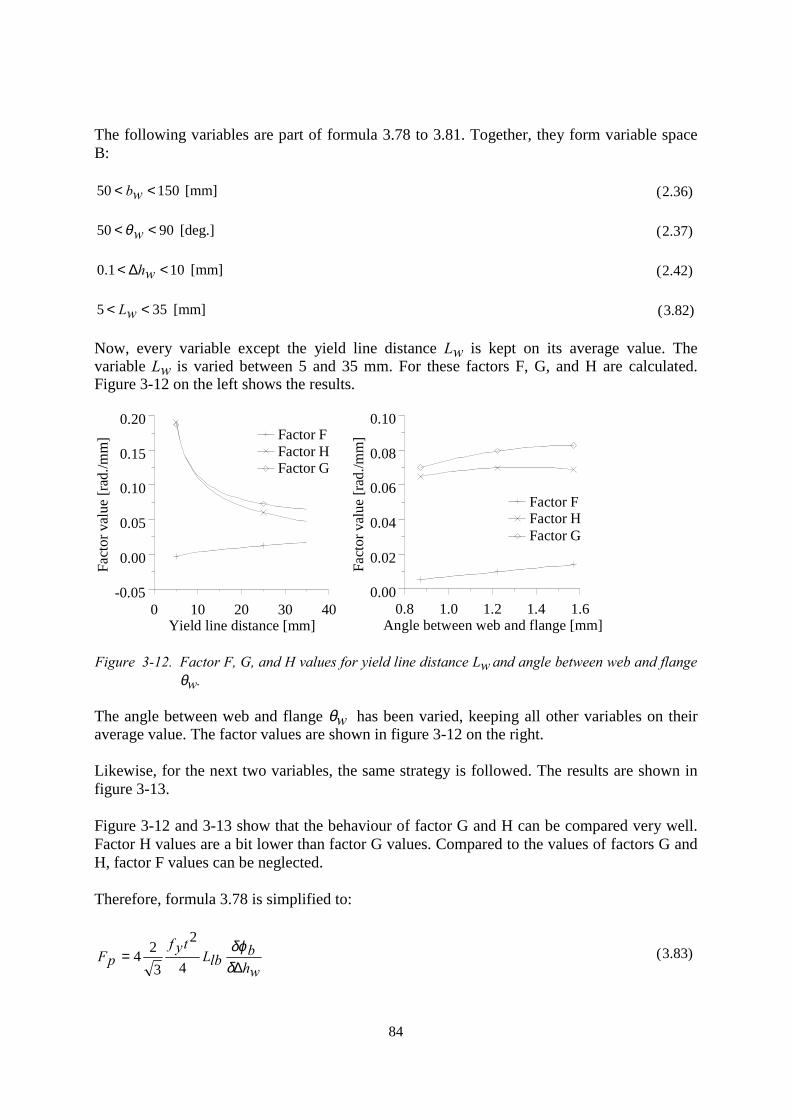
84
The following variables are part of formula 3.78 to 3.81. Together, they form variable spaceB:
15050 << wb [mm] (2.36)
9050 << wθ [deg.] (2.37)
101.0 <∆< wh [mm] (2.42)
355 << wL [mm] (3.82)
Now, every variable except the yield line distance Lw is kept on its average value. Thevariable Lw is varied between 5 and 35 mm. For these factors F, G, and H are calculated.Figure 3-12 on the left shows the results.
0 10 20 30 40Yield line distance [mm]
-0.05
0.00
0.05
0.10
0.15
0.20
Fact
or v
alue
[rad
./mm
] Factor FFactor HFactor G
0.8 1.0 1.2 1.4 1.6Angle between web and flange [mm]
0.00
0.02
0.04
0.06
0.08
0.10
Fact
or v
alue
[rad
./mm
]
Factor FFactor HFactor G
Figure 3-12. Factor F, G, and H values for yield line distance Lw and angle between web and flangeθw.
The angle between web and flange θw has been varied, keeping all other variables on theiraverage value. The factor values are shown in figure 3-12 on the right.
Likewise, for the next two variables, the same strategy is followed. The results are shown infigure 3-13.
Figure 3-12 and 3-13 show that the behaviour of factor G and H can be compared very well.Factor H values are a bit lower than factor G values. Compared to the values of factors G andH, factor F values can be neglected.
Therefore, formula 3.78 is simplified to:
whb
lbLtyf
pF∆
=δδϕ
4
2
324 (3.83)
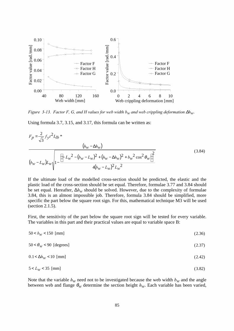
85
40 80 120 160Web width [mm]
0.00
0.02
0.04
0.06
0.08
0.10
Fact
or v
alue
[rad
./mm
]
0 2 4 6 8 10Web crippling deformation [mm]
0.0
0.2
0.4
0.6
Fact
or v
alue
[rad
./mm
]
Factor FFactor HFactor G
Factor FFactor HFactor G
Figure 3-13. Factor F, G, and H values for web width bw and web crippling deformation ∆hw.
Using formula 3.7, 3.15, and 3.17, this formula can be written as:
( )
( )( ) ( )
( ) 224
22cos22221
*23
2
wLwLwb
wwbwhwhwLwbwLwLwLwb
whwh
lbLtyfpF
−
+∆−+−−−−−
∆−
=
θ(3.84)
If the ultimate load of the modelled cross-section should be predicted, the elastic and theplastic load of the cross-section should be set equal. Therefore, formulae 3.77 and 3.84 shouldbe set equal. Hereafter, ∆hw should be solved. However, due to the complexity of formulae3.84, this is an almost impossible job. Therefore, formula 3.84 should be simplified, morespecific the part below the square root sign. For this, mathematical technique M3 will be used(section 2.1.5).
First, the sensitivity of the part below the square root sign will be tested for every variable.The variables in this part and their practical values are equal to variable space B:
15050 << wb [mm] (2.36)
9050 << wθ [degrees] (2.37)
101.0 <∆< wh [mm] (2.42)
355 << wL [mm] (3.82)
Note that the variable hw need not to be investigated because the web width bw and the anglebetween web and flange θw determine the section height hw. Each variable has been varied,
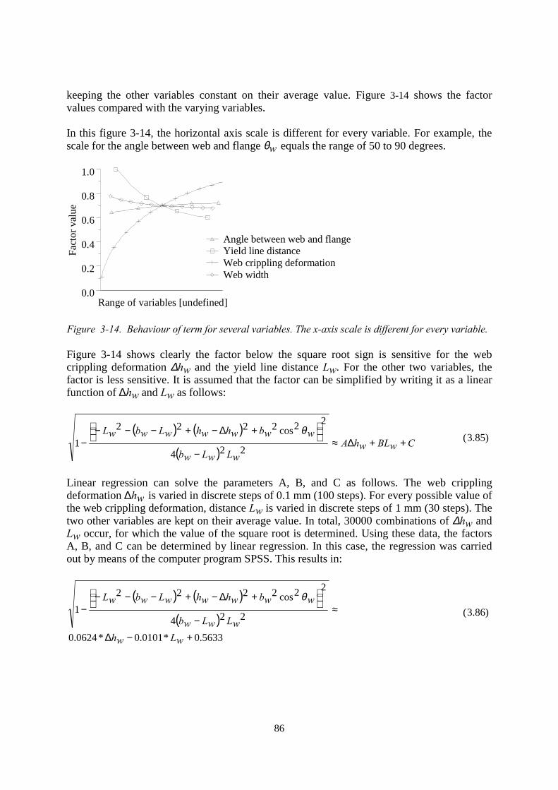
86
keeping the other variables constant on their average value. Figure 3-14 shows the factorvalues compared with the varying variables.
In this figure 3-14, the horizontal axis scale is different for every variable. For example, thescale for the angle between web and flange θw equals the range of 50 to 90 degrees.
0.0
0.2
0.4
0.6
0.8
1.0
Range of variables [undefined]
Fact
or v
alue
Angle between web and flangeYield line distanceWeb crippling deformationWeb width
Figure 3-14. Behaviour of term for several variables. The x-axis scale is different for every variable.
Figure 3-14 shows clearly the factor below the square root sign is sensitive for the webcrippling deformation ∆hw and the yield line distance Lw. For the other two variables, thefactor is less sensitive. It is assumed that the factor can be simplified by writing it as a linearfunction of ∆hw and Lw as follows:
( ) ( )
( )CwBLwhA
wLwLwb
wwbwhwhwLwbwL++∆≈
−
+∆−+−−−−
224
22cos22221
θ(3.85)
Linear regression can solve the parameters A, B, and C as follows. The web cripplingdeformation ∆hw is varied in discrete steps of 0.1 mm (100 steps). For every possible value ofthe web crippling deformation, distance Lw is varied in discrete steps of 1 mm (30 steps). Thetwo other variables are kept on their average value. In total, 30000 combinations of ∆hw andLw occur, for which the value of the square root is determined. Using these data, the factorsA, B, and C can be determined by linear regression. In this case, the regression was carriedout by means of the computer program SPSS. This results in:
( ) ( )
( )5633.0*0101.0*0624.0
224
22cos22221
+−∆
≈−
+∆−+−−−−
wLwhwLwLwb
wwbwhwhwLwbwL θ(3.86)
87
Formula 3.86 can be substituted into formula 3.84 that results in:
( )( ) ( ) ( ) ( )( )5633.00101.00624.0
2+−+∆−
∆−=
wLwhwLwLwbwhwh
lbLtyfpF (3.87)
Setting equal formulae 3.77 and 3.87 (and thus equal elastic and plastic behaviour of thecross-section) makes it possible to solve ∆hw. For this purpose, some parts of the formulae arerenamed.
( ) ( ) ( ) ( )( )
( )( ) ( )
⇔
−
∆+
=++∆−
∆−
sin
34*2sin2
23
5633.00101.00624.02
wibfrbfbwbwibfr
whwbbfbEI
wLwhwLwLwbwhwh
lbLtyf
θθ
( ) ( ) ⇔∆=++∆−
∆−whk
CwBLwhAwLwLwbwhwh
lbLtyf 2
( ) ( )( ) wLwLwbAk
twLwLwblbkLwhyAfwh
−
+−−−=∆
2
224 φφ (3.88)
2322 tlbLyfwBkLwCkLwkLwBbwCkLwb +−−+=φ (3.89)
In the last derivation, k is defined as the elastic web crippling stiffness. Therefore, formula2.44 has been derived. Now, the ultimate load of the modelled cross-section Fcsu can easilybe determined by calculating Fp or Fe for solved ∆hw. Furthermore, the factor φ can berewritten as follows:
=+−−+= 2322 tlbLyfwBkLwCkLwkLwBbwCkLwbφ
=+
−−+= 22 tlbLyfwBLwCLwLwBbCwbwkL
( ) ( )( ) =+−+−= 2tlbLyfwLwbwBLwLwbCwkL
( )( ) =+−+= 2tlbLyfwLwbwBLCwkL
αβ += (3.90)
88
2tlbLyf=α (3.91)
( )( )wLwbwBLCwkL −+=β (3.92)
Thus, load Fcsu can be described as follows:
( ) ( )( ) wLwLwbA
kwLwLwbwhAwhkcsuF
−++−+−−
=∆=2
24 αβαβα (3.93)
Formulae 3.91, 3.92, and 3.93 are equal to formulae 2.45, 2.46, and 2.43 in appendix 2.Formulae 2.47, 2.48, and 2.49 can be derived from formulae 3.85 and 3.86.
3.7 Derivation of formula 2.53
Formula 3.28 describes the web crippling deformation ∆hw as a function of the rotation ϕ. Ifit assumed that the rotation ϕ is small (out of the experimental data it can be shown that ϕ willnot exceed 5 degrees at failure), the following can be stated.
ϕϕ ≈sin (3.94)
1cos ≈ϕ (3.95)
Using the two formulae presented above, formula 3.28 can be rewritten.
( ) ( ) ( ) ϕϕϕϕ bfLwhbfLbfLwhwhbfLbfLbfLwhwh -22 22 −−=+−−++−=∆ (3.96)
Now, the rotation ϕ can be solved straightforward:
( ) ( ) ( ) ⇔−−=+∆⇔−−+−=∆ 22222 ϕϕϕϕ whbfLbfLbfLwhwhbfLbfLbfLwh
⇔−+−=+∆+∆ 222222222 ϕϕϕϕ whwhbfLbfLbfLbfLbfLwhwh
⇔=+−+∆+∆ 02222222 ϕϕϕϕ whbfLwhbfLbfLwhwh
( )( ) ⇔=
∆+−∆+
+ 022222whwhwhbfLwhbfL ϕϕ
( )( ) ( )( )
+
∆
+−−∆±−∆−=
222
2224222
whbfL
whwhbfLwhwhbfLwhwhbfLϕ (3.97)
89
This simple prediction of rotation ϕ can be derived to ∆hw, however, this leads to acomplicated formula. Instead, formula 3.27 and 3.33 are used, assuming a small rotation ϕ:
( )
( )⇒
−−=
∆−−=
∆
2sincos2
22
ϕϕ
δδϕ
whbfLbfLtfw
whwhtfwbfL
tfw
wh
( )( )( )
( )( )( )whwhwhbfL
whbfLbfL
whwhwhbfLwhbfLbfL
wh ∆−−
−−≈
∆−−
−−=
∆ ϕ
ϕ
ϕϕ
ϕϕ
δδϕ
22
sincos
2sincos2(3.98)
Using formula 2.32 the first length factor fl1 can now be written as:
( )( )( )whwhwhbfL
whbfLbfLlbLspanLlf
∆−−
−−
−+
=
ϕ
ϕ 22
21
11
(3.99)
This formula equals formula 2.53 in appendix 2.
3.8 Derivation of formula 2.57
Appendix 2 shows that the sheet section ultimate load Fu can be calculated using more or lessrefinement (model MA1 to MA12, MR1 to MR12, and ME1). The distance between yieldlines Lbf can be found by minimising Fu to Lbf, in other words to find a distance Lbf forwhich Fu will be as small as possible. Although the ultimate load Fu can be predicted byformula 2.54, a very complex one, it is nearly impossible to minimise Lbf using this formula.Deriving the length factor fl1 to Lbf is an almost impossible job. Therefore, the followingstrategy is followed. Why not chose a simple formula predicting Fu to determine Lbf, even ifa complex formula is used to predicting Fu itself? The only thing that should be considered isto choose such a simple formula predicting Fu that it makes sense to minimise Lbf. Thissituation can be found for formula 2.65. Common sense dictates that F2p and Fylbf should beconsidered during a Lbf determination. These loads predict the extra forces that are needed todeform the sections adjacent to the modelled cross-section. The length factor is not includedfor formula 2.65. Although this is theoretically not correct, it’s derivation will result intolengthy formulae. Besides this aspect, common sense again dictates that the length factor willbe less influenced by Lbf than the parts that directly relate their widths to Lbf. If Lbfdetermination will be successful using formula 2.65, the length factor relationship to Lbf willindeed be considered unimportant. If not, reconsideration of the above mentioned strategysurely will be needed. Looking at formula 2.65, the derivative to Lbf equals:
bfLylbfF
bfLpF
bfLcsuF
bfLuF
δδ
δδ
δδ
δδ
++= 2(3.100)
90
This derivative should be zero to find the minimal Fu. Furthermore, formula 3.93 shows Fcsuis not a function of Lbf. Therefore:
bfLylbfF
bfLpF
δδ
δδ
+= 20 (3.101)
For convenience, the function predicting F2p and Fylbf will be presented here again. ForFylbf, formula 2.26 is used.
lbLbfL
csuFpF =2 (2.50)
∆
+∆
=whe
whd
bfbtyf
ylbfFδδϕ
δδϕ
4
2
322 (2.26)
The derivative of formula 2.50 can be presented straightforward:
lbLcsuF
bfLpF
=δδ 2
(3.102)
Although the derivative of formula 2.26 can be derived, this leads to complex formulae.Therefore, a linear approximation of Fylbf will be used. Formula 2.26 will first be simplifiedusing mathematical technique M3: make complex functions linear. Lbf and ∆hw will differ asfollows:
[mm] 9510 << bfL (3.103)
[mm] 81.0 <∆< wh (3.104)
Now, Fylbf is written as:
+∆+≈ 2
4
2
322 CwhB
bfLA
bfbtyf
ylbfF (3.105)
Linear regression can solve the parameters A, B, and C as follows. The web cripplingdeformation ∆hw is varied in discrete steps of 0.8 mm (10 steps). For every possible value ofthe web crippling deformation, distance Lbf is varied in discrete steps of 8.5 mm (10 steps). Intotal, 100 combinations of ∆hw and Lbf occur, for which the value of Fylbf is determined.Using these data, the factors A, B, and C can be determined by linear regression.
91
This results in:
019.02000393.0601.24
2
322
−∆+≈ wh
bfLbfbtyf
ylbfF (3.106)
The above-presented formula has a correlation of 0.951 to the standard formula for the dataused. To try the suggestion that Fylbf is not seriously influenced by ∆hw, a new simplifiedformula is proposed:
4
2
322
+≈ B
bfLA
bfbtyf
ylbfF (3.107)
Using the computer program and the data, factors A and B are:
001.0601.24
2
322
−≈
bfLbfbtyf
ylbfF (3.108)
The above-presented formula has a correlation of 0.944 to the standard formula. Thederivative of this formula to Lbf equals:
2601.2
4
2
322
bfLbfb
tyf
bfLylbfF
−≈δ
δ(3.109)
Substituting formula 3.102 and 3.109 into 3.101 leads to:
( ) ⇔−=2
601.24
2
3220
bfLbfb
tyf
lbLcsuF
csuFbfblbLtyf
bfL4
601.222= (3.110)
The last formula equals formula 2.57 in appendix 2.
3.9 Derivation of formulae 2.74 and 2.75
Formula 3.43 showed how the plastic load for the rolling post-failure mode can be calculated.Now this formula will be rewritten as built up out of components:
KJIpF ++= (3.111)
92
With:
lbLtyf
bfrwhau
I4
2
3212
∆=
δδ (3.112)
lbLtyf
bfrwhbu
J4
2
3212
∆=
δδ (3.113)
lbLtyf
whcK
4
2
322
∆=
δδϕ (3.114)
Component K can be calculated using formula 3.50, 3.55, and 3.68. For the derivation offormula 3.68, it was assumed that angle ϕc is small and corner radius rbf equals zero. Thisalso applies for formula 3.50:
( )( ) ( )wcw
wcwflbwflb
θϕθθϕ
sincos1
sin
+−≈∆ (3.115)
Component I and J can be calculated using formulae 3.56 and 3.57. These formulae can berewritten in the same way as for formula 3.50:
( )( )
( ) ( )( ) ( )wcw
wcwcw
cwwhau
θϕθθϕθ
ϕθϕθ
δδ
sincos1cossin
cos1sin
+−+
≈+−
+=
∆ (3.116)
( )( )
( ) ( )( ) ( )wcw
wcwwflb-wflb
bfr
cwcw
whbu
θϕθθϕθ
ϕθϕθ
δδ
sincos1cossin
cos1sin
+−+
≈∆
++−
+=
∆(3.117)
For all variables, defined variable space A is used (section 2.2.3):
15050 << wb [mm]. (2.36)
9050 << wθ [degrees]. (2.37)
15050 << lbL [mm]. (2.38)
5.15.0 << t [mm]. (2.39)
15040 << bfb [mm]. (2.40)
121 << bfr [mm]. (2.41)
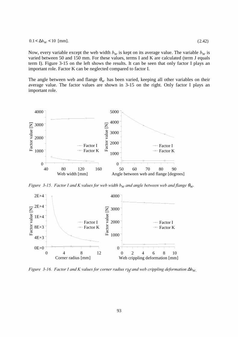
93
101.0 <∆< wh [mm]. (2.42)
Now, every variable except the web width bw is kept on its average value. The variable bw isvaried between 50 and 150 mm. For these values, terms I and K are calculated (term J equalsterm I). Figure 3-15 on the left shows the results. It can be seen that only factor I plays animportant role. Factor K can be neglected compared to factor I.
The angle between web and flange θw has been varied, keeping all other variables on theiraverage value. The factor values are shown in 3-15 on the right. Only factor I plays animportant role.
40 80 120 160Web width [mm]
0
1000
2000
3000
4000
Fact
or v
alue
[N]
50 60 70 80 90Angle between web and flange [degrees]
0
1000
2000
3000
4000
5000Fa
ctor
val
ue [N
]
Factor IFactor K
Factor IFactor K
Figure 3-15. Factor I and K values for web width bw and angle between web and flange θw.
0 4 8 12Corner radius [mm]
0E+0
4E+3
8E+3
1E+4
2E+4
2E+4
Fact
or v
alue
[N]
0 2 4 6 8 10Web crippling deformation [mm]
0
1000
2000
3000
4000
Fact
or v
alue
[N]
Factor IFactor K
Factor IFactor K
Figure 3-16. Factor I and K values for corner radius rbf and web crippling deformation ∆hw.
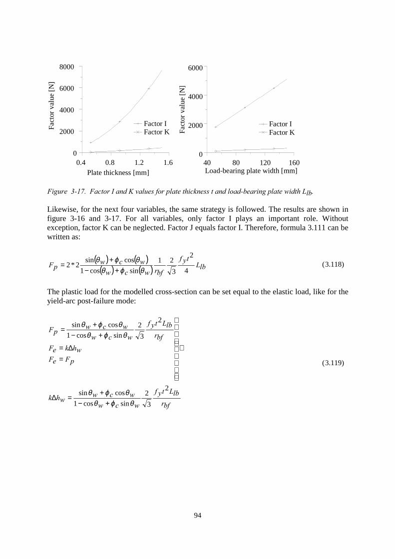
94
0.4 0.8 1.2 1.6Plate thickness [mm]
0
2000
4000
6000
8000
Fact
or v
alue
[N]
40 80 120 160Load-bearing plate width [mm]
0
2000
4000
6000
Fact
or v
alue
[N]
Factor IFactor K
Factor IFactor K
Figure 3-17. Factor I and K values for plate thickness t and load-bearing plate width Llb.
Likewise, for the next four variables, the same strategy is followed. The results are shown infigure 3-16 and 3-17. For all variables, only factor I plays an important role. Withoutexception, factor K can be neglected. Factor J equals factor I. Therefore, formula 3.111 can bewritten as:
( ) ( )( ) ( ) lbL
tyf
bfrwcwwcw
pF4
2
321
sincos1cossin
2*2θϕθ
θϕθ+−
+= (3.118)
The plastic load for the modelled cross-section can be set equal to the elastic load, like for theyield-arc post-failure mode:
bfrlbLtyf
wcwwcw
whk
pFeFwhkeF
bfrlbLtyf
wcwwcw
pF
2
32
sincos1cossin
2
32
sincos1cossin
θϕθθϕθ
θϕθθϕθ
+−+
=∆
⇒
=∆=
+−+
=
(3.119)
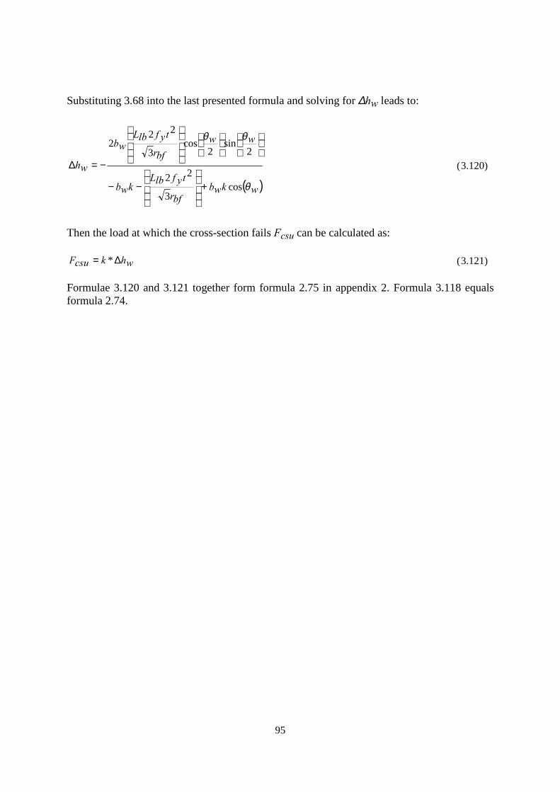
95
Substituting 3.68 into the last presented formula and solving for ∆hw leads to:
( )
cos3
22
2sin
2cos
3
222
wkwbbfr
tyflbLkwb
wwbfr
tyflbLwb
wh
θ
θθ
+
−−
−=∆ (3.120)
Then the load at which the cross-section fails Fcsu can be calculated as:
* whkcsuF ∆= (3.121)
Formulae 3.120 and 3.121 together form formula 2.75 in appendix 2. Formula 3.118 equalsformula 2.74.

96
4 Appendix cross-section behaviour
IntroductionThe experiments in chapter 3 of thesis [Hofm00a] indicated that for a large concentrated loadand a small bending moment (short span lengths), two post-failure modes could occur: therolling and the yield arc post-failure modes, see also table 3-7, thesis [Hofm00a]. Research inthe past indicated that the corner radius has a strong influence on which of these two post-failure modes occurs [Bakk92a], [Hofm96a].
In this appendix, it has been investigated whether small strips of the sheet section's cross-section can be used to gather insight into the differences of the two post-failure modes. Forsmall corner radii, it will be shown that strip behaviour and section behaviour is comparable.For large corner radii, this is not the case.
Finite element models have been used to describe the cross-sectional behaviour of sheetsections for varying corner radii. Relatively simple mechanical models have been derived thatdetermine the location of first yield in the cross-section's web and the cross-section's plasticbehaviour. Except for the largest corner radius, mechanical models and finite element modelsgive comparable results.
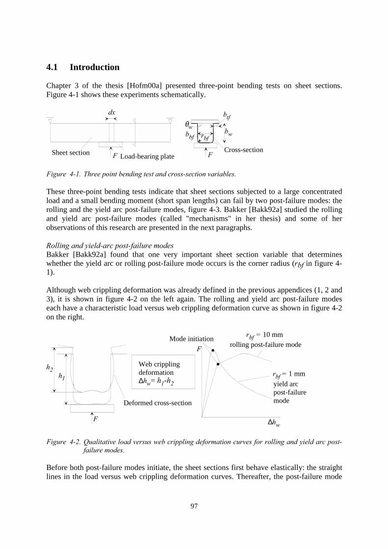
97
4.1 Introduction
Chapter 3 of the thesis [Hofm00a] presented three-point bending tests on sheet sections.Figure 4-1 shows these experiments schematically.
dx
FSheet section Load-bearing plate
bbf rbfbw
F
θw
btf
Cross-section
Figure 4-1. Three point bending test and cross-section variables.
These three-point bending tests indicate that sheet sections subjected to a large concentratedload and a small bending moment (short span lengths) can fail by two post-failure modes: therolling and the yield arc post-failure modes, figure 4-3. Bakker [Bakk92a] studied the rollingand yield arc post-failure modes (called "mechanisms" in her thesis) and some of herobservations of this research are presented in the next paragraphs.
Rolling and yield-arc post-failure modesBakker [Bakk92a] found that one very important sheet section variable that determineswhether the yield arc or rolling post-failure mode occurs is the corner radius (rbf in figure 4-1).
Although web crippling deformation was already defined in the previous appendices (1, 2 and3), it is shown in figure 4-2 on the left again. The rolling and yield arc post-failure modeseach have a characteristic load versus web crippling deformation curve as shown in figure 4-2on the right.
F
Deformed cross-section
Web cripplingdeformation
F rolling post-failure mode
yield arcpost-failuremode
Mode initiation
∆hw
∆hw= h1-h2h1
h2 rbf = 1 mm
rbf = 10 mm
Figure 4-2. Qualitative load versus web crippling deformation curves for rolling and yield arc post-failure modes.
Before both post-failure modes initiate, the sheet sections first behave elastically: the straightlines in the load versus web crippling deformation curves. Thereafter, the post-failure mode
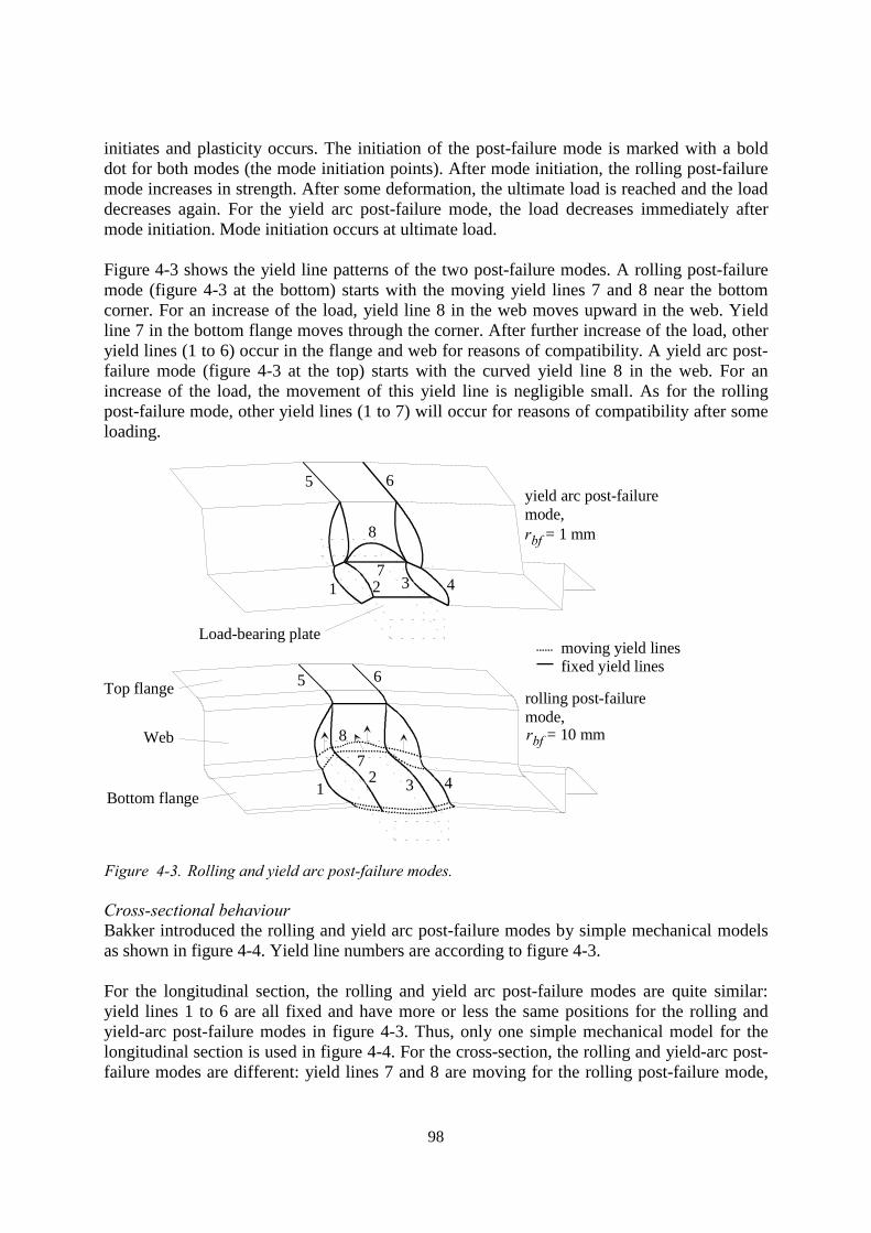
98
initiates and plasticity occurs. The initiation of the post-failure mode is marked with a bolddot for both modes (the mode initiation points). After mode initiation, the rolling post-failuremode increases in strength. After some deformation, the ultimate load is reached and the loaddecreases again. For the yield arc post-failure mode, the load decreases immediately aftermode initiation. Mode initiation occurs at ultimate load.
Figure 4-3 shows the yield line patterns of the two post-failure modes. A rolling post-failuremode (figure 4-3 at the bottom) starts with the moving yield lines 7 and 8 near the bottomcorner. For an increase of the load, yield line 8 in the web moves upward in the web. Yieldline 7 in the bottom flange moves through the corner. After further increase of the load, otheryield lines (1 to 6) occur in the flange and web for reasons of compatibility. A yield arc post-failure mode (figure 4-3 at the top) starts with the curved yield line 8 in the web. For anincrease of the load, the movement of this yield line is negligible small. As for the rollingpost-failure mode, other yield lines (1 to 7) will occur for reasons of compatibility after someloading.
moving yield linesfixed yield lines
rolling post-failuremode,
yield arc post-failuremode,
Top flange
Web
Bottom flange 12 3 4
5 6
1 2 3 4
5 6
78
7
8
Load-bearing plate
rbf = 1 mm
rbf = 10 mm
Figure 4-3. Rolling and yield arc post-failure modes.
Cross-sectional behaviourBakker introduced the rolling and yield arc post-failure modes by simple mechanical modelsas shown in figure 4-4. Yield line numbers are according to figure 4-3.
For the longitudinal section, the rolling and yield arc post-failure modes are quite similar:yield lines 1 to 6 are all fixed and have more or less the same positions for the rolling andyield-arc post-failure modes in figure 4-3. Thus, only one simple mechanical model for thelongitudinal section is used in figure 4-4. For the cross-section, the rolling and yield-arc post-failure modes are different: yield lines 7 and 8 are moving for the rolling post-failure mode,
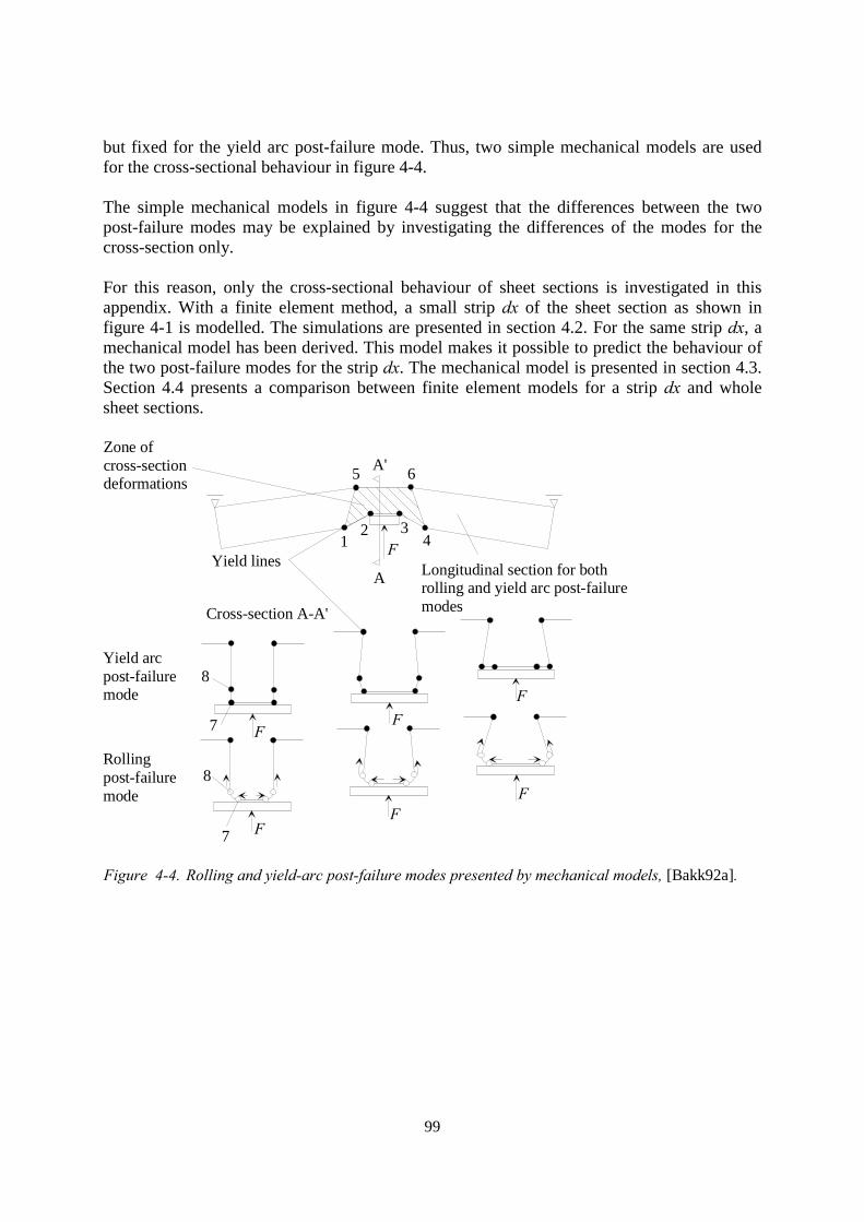
99
but fixed for the yield arc post-failure mode. Thus, two simple mechanical models are usedfor the cross-sectional behaviour in figure 4-4.
The simple mechanical models in figure 4-4 suggest that the differences between the twopost-failure modes may be explained by investigating the differences of the modes for thecross-section only.
For this reason, only the cross-sectional behaviour of sheet sections is investigated in thisappendix. With a finite element method, a small strip dx of the sheet section as shown infigure 4-1 is modelled. The simulations are presented in section 4.2. For the same strip dx, amechanical model has been derived. This model makes it possible to predict the behaviour ofthe two post-failure modes for the strip dx. The mechanical model is presented in section 4.3.Section 4.4 presents a comparison between finite element models for a strip dx and wholesheet sections.
F
Yield arcpost-failuremode
Rollingpost-failuremode
Longitudinal section for bothrolling and yield arc post-failuremodesCross-section A-A'
A
A'Zone ofcross-sectiondeformations
Yield lines1
2 34
5 6
7
8
8
7 F
FF
F
FF
Figure 4-4. Rolling and yield-arc post-failure modes presented by mechanical models, [Bakk92a].
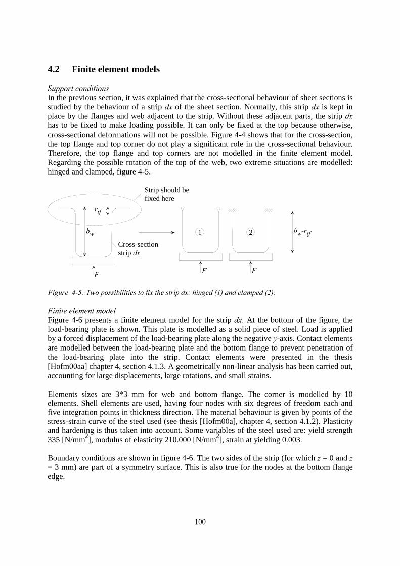
100
4.2 Finite element models
Support conditionsIn the previous section, it was explained that the cross-sectional behaviour of sheet sections isstudied by the behaviour of a strip dx of the sheet section. Normally, this strip dx is kept inplace by the flanges and web adjacent to the strip. Without these adjacent parts, the strip dxhas to be fixed to make loading possible. It can only be fixed at the top because otherwise,cross-sectional deformations will not be possible. Figure 4-4 shows that for the cross-section,the top flange and top corner do not play a significant role in the cross-sectional behaviour.Therefore, the top flange and top corners are not modelled in the finite element model.Regarding the possible rotation of the top of the web, two extreme situations are modelled:hinged and clamped, figure 4-5.
Cross-section strip dx
Strip should be fixed here
F F
1 2bw
rtf
bw-rtf
F
Figure 4-5. Two possibilities to fix the strip dx: hinged (1) and clamped (2).
Finite element modelFigure 4-6 presents a finite element model for the strip dx. At the bottom of the figure, theload-bearing plate is shown. This plate is modelled as a solid piece of steel. Load is appliedby a forced displacement of the load-bearing plate along the negative y-axis. Contact elementsare modelled between the load-bearing plate and the bottom flange to prevent penetration ofthe load-bearing plate into the strip. Contact elements were presented in the thesis[Hofm00aa] chapter 4, section 4.1.3. A geometrically non-linear analysis has been carried out,accounting for large displacements, large rotations, and small strains.
Elements sizes are 3*3 mm for web and bottom flange. The corner is modelled by 10elements. Shell elements are used, having four nodes with six degrees of freedom each andfive integration points in thickness direction. The material behaviour is given by points of thestress-strain curve of the steel used (see thesis [Hofm00a], chapter 4, section 4.1.2). Plasticityand hardening is thus taken into account. Some variables of the steel used are: yield strength335 [N/mm2], modulus of elasticity 210.000 [N/mm2], strain at yielding 0.003.
Boundary conditions are shown in figure 4-6. The two sides of the strip (for which z = 0 and z= 3 mm) are part of a symmetry surface. This is also true for the nodes at the bottom flangeedge.
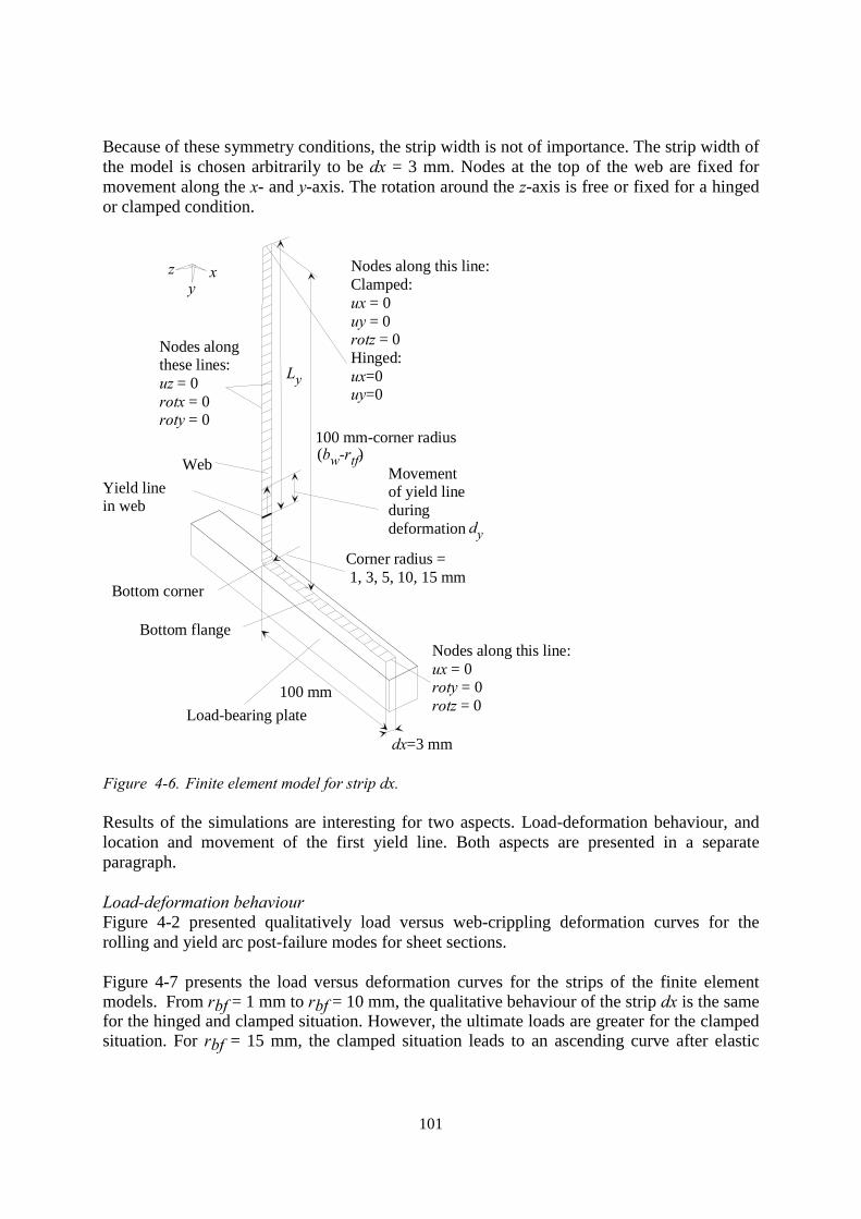
101
Because of these symmetry conditions, the strip width is not of importance. The strip width ofthe model is chosen arbitrarily to be dx = 3 mm. Nodes at the top of the web are fixed formovement along the x- and y-axis. The rotation around the z-axis is free or fixed for a hingedor clamped condition.
100 mm-corner radius
100 mm
Corner radius = 1, 3, 5, 10, 15 mm
Load-bearing plate
Bottom flange
Web
Bottom corner
Nodes along this line:Clamped:ux = 0uy = 0rotz = 0Hinged:ux=0uy=0
Nodes alongthese lines:uz = 0rotx = 0roty = 0
dx=3 mm
Nodes along this line:ux = 0roty = 0rotz = 0
xzy
(bw-rtf)
Ly
Yield linein web
Movementof yield lineduringdeformation dy
Figure 4-6. Finite element model for strip dx.
Results of the simulations are interesting for two aspects. Load-deformation behaviour, andlocation and movement of the first yield line. Both aspects are presented in a separateparagraph.
Load-deformation behaviourFigure 4-2 presented qualitatively load versus web-crippling deformation curves for therolling and yield arc post-failure modes for sheet sections.
Figure 4-7 presents the load versus deformation curves for the strips of the finite elementmodels. From rbf = 1 mm to rbf = 10 mm, the qualitative behaviour of the strip dx is the samefor the hinged and clamped situation. However, the ultimate loads are greater for the clampedsituation. For rbf = 15 mm, the clamped situation leads to an ascending curve after elastic
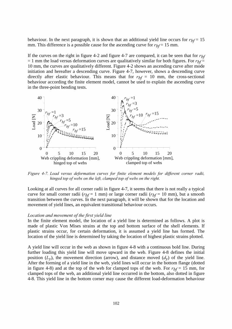
102
behaviour. In the next paragraph, it is shown that an additional yield line occurs for rbf = 15mm. This difference is a possible cause for the ascending curve for rbf = 15 mm.
If the curves on the right in figure 4-2 and figure 4-7 are compared, it can be seen that for rbf= 1 mm the load versus deformation curves are qualitatively similar for both figures. For rbf =10 mm, the curves are qualitatively different. Figure 4-2 shows an ascending curve after modeinitiation and hereafter a descending curve. Figure 4-7, however, shows a descending curvedirectly after elastic behaviour. This means that for rbf = 10 mm, the cross-sectionalbehaviour according the finite element model, cannot be used to explain the ascending curvein the three-point bending tests.
0 5 10 15 20Web crippling deformation [mm],
hinged top of webs
0
10
20
30
40
rbf =1
0 5 10 15 20Web crippling deformation [mm],
clamped top of webs
0
10
20
30
40
Load
[N] rbf =3
rbf =5rbf =10
rbf =15 Load
[N]
rbf =1rbf =3rbf =5
rbf =10 rbf =15
Figure 4-7. Load versus deformation curves for finite element models for different corner radii,hinged top of webs on the left, clamped top of webs on the right.
Looking at all curves for all corner radii in figure 4-7, it seems that there is not really a typicalcurve for small corner radii (rbf = 1 mm) or large corner radii (rbf = 10 mm), but a smoothtransition between the curves. In the next paragraph, it will be shown that for the location andmovement of yield lines, an equivalent transitional behaviour occurs.
Location and movement of the first yield lineIn the finite element model, the location of a yield line is determined as follows. A plot ismade of plastic Von Mises strains at the top and bottom surface of the shell elements. Ifplastic strains occur, for certain deformation, it is assumed a yield line has formed. Thelocation of the yield line is determined by taking the location of highest plastic strains plotted.
A yield line will occur in the web as shown in figure 4-8 with a continuous bold line. Duringfurther loading this yield line will move upward in the web. Figure 4-8 defines the initialposition (Ly), the movement direction (arrow), and distance moved (dy) of the yield line.After the forming of a yield line in the web, yield lines will occur in the bottom flange (dottedin figure 4-8) and at the top of the web for clamped tops of the web. For rbf = 15 mm, forclamped tops of the web, an additional yield line occurred in the bottom, also dotted in figure4-8. This yield line in the bottom corner may cause the different load-deformation behaviour
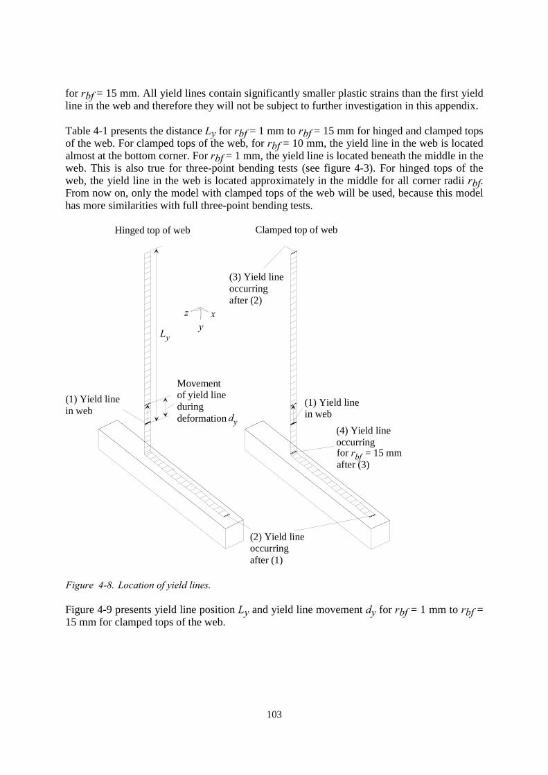
103
for rbf = 15 mm. All yield lines contain significantly smaller plastic strains than the first yieldline in the web and therefore they will not be subject to further investigation in this appendix.
Table 4-1 presents the distance Ly for rbf = 1 mm to rbf = 15 mm for hinged and clamped topsof the web. For clamped tops of the web, for rbf = 10 mm, the yield line in the web is locatedalmost at the bottom corner. For rbf = 1 mm, the yield line is located beneath the middle in theweb. This is also true for three-point bending tests (see figure 4-3). For hinged tops of theweb, the yield line in the web is located approximately in the middle for all corner radii rbf.From now on, only the model with clamped tops of the web will be used, because this modelhas more similarities with full three-point bending tests.
Ly
(1) Yield linein web
Movementof yield lineduringdeformation
(2) Yield lineoccurringafter (1)
(4) Yield lineoccurring
(3) Yield lineoccurringafter (2)
(1) Yield linein webdy
Hinged top of web Clamped top of web
xy
z
for rbf = 15 mmafter (3)
Figure 4-8. Location of yield lines.
Figure 4-9 presents yield line position Ly and yield line movement dy for rbf = 1 mm to rbf =15 mm for clamped tops of the web.
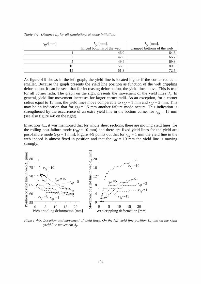
104
Table 4-1. Distance Ly for all simulations at mode initiation.
rbf [mm] Ly [mm],hinged bottoms of the web
Ly [mm],clamped bottoms of the web
1 46.0 64.33 47.0 66.25 49.4 69.8
10 56.5 80.015 61.3 72.5
As figure 4-9 shows in the left graph, the yield line is located higher if the corner radius issmaller. Because the graph presents the yield line position as function of the web cripplingdeformation, it can be seen that for increasing deformation, the yield lines move. This is truefor all corner radii. The graph on the right presents the movement of the yield lines dy. Ingeneral, yield line movement increases for larger corner radii. As an exception, for a cornerradius equal to 15 mm, the yield lines move comparable to rbf = 1 mm and rbf = 3 mm. Thismay be an indication that for rbf = 15 mm another failure mode occurs. This indication isstrengthened by the occurrence of an extra yield line in the bottom corner for rbf = 15 mm(see also figure 4-8 on the right).
In section 4.1, it was mentioned that for whole sheet sections, there are moving yield lines forthe rolling post-failure mode (rbf = 10 mm) and there are fixed yield lines for the yield arcpost-failure mode (rbf = 1 mm). Figure 4-9 points out that for rbf = 1 mm the yield line in theweb indeed is almost fixed in position and that for rbf = 10 mm the yield line is movingstrongly.
0 5 10 15 20Web crippling deformation [mm]
55
60
65
70
75
80
Posi
tion
of y
ield
line
in w
eb L
y [m
m]
rbf =10
rbf =15
rbf =1rbf =3
rbf =5
0 5 10 15 20Web crippling deformation [mm]
0
4
8
12
16
20
Mov
emen
t of y
ield
line
in w
eb d
y [m
m]
rbf =10
rbf =3
rbf =1
rbf =15
rbf =5
Figure 4-9. Location and movement of yield lines. On the left yield line position Ly and on the rightyield line movement dy.
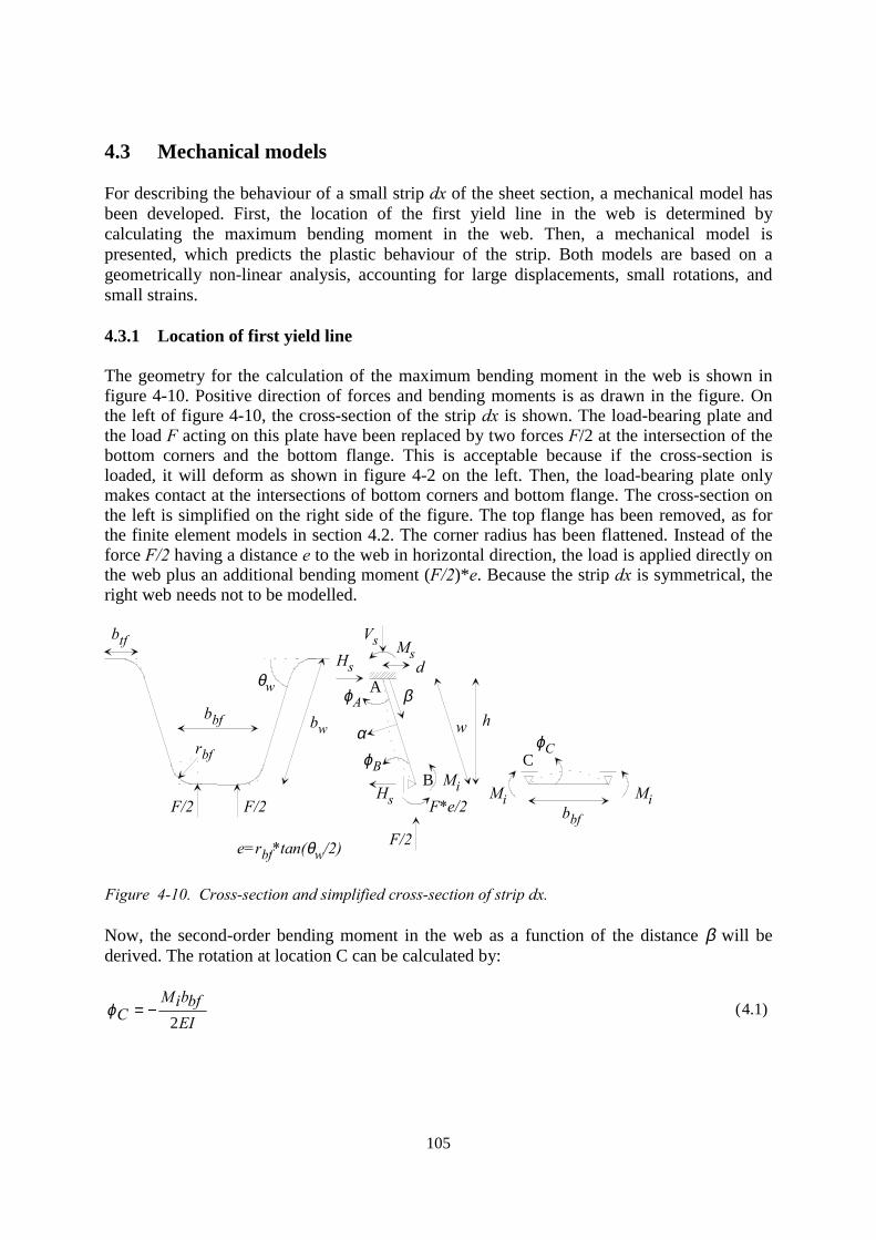
105
4.3 Mechanical models
For describing the behaviour of a small strip dx of the sheet section, a mechanical model hasbeen developed. First, the location of the first yield line in the web is determined bycalculating the maximum bending moment in the web. Then, a mechanical model ispresented, which predicts the plastic behaviour of the strip. Both models are based on ageometrically non-linear analysis, accounting for large displacements, small rotations, andsmall strains.
4.3.1 Location of first yield line
The geometry for the calculation of the maximum bending moment in the web is shown infigure 4-10. Positive direction of forces and bending moments is as drawn in the figure. Onthe left of figure 4-10, the cross-section of the strip dx is shown. The load-bearing plate andthe load F acting on this plate have been replaced by two forces F/2 at the intersection of thebottom corners and the bottom flange. This is acceptable because if the cross-section isloaded, it will deform as shown in figure 4-2 on the left. Then, the load-bearing plate onlymakes contact at the intersections of bottom corners and bottom flange. The cross-section onthe left is simplified on the right side of the figure. The top flange has been removed, as forthe finite element models in section 4.2. The corner radius has been flattened. Instead of theforce F/2 having a distance e to the web in horizontal direction, the load is applied directly onthe web plus an additional bending moment (F/2)*e. Because the strip dx is symmetrical, theright web needs not to be modelled.
bw
θw
btf
bbf
rbf
F/2 F/2
MsVs
Hs
w
Hs
F/2
F*e/2
e=rbf*tan(θw/2)
Mi
ϕB
ϕA
α
βh
d
bbf
Mi Mi
ϕCC
B
A
Figure 4-10. Cross-section and simplified cross-section of strip dx.
Now, the second-order bending moment in the web as a function of the distance β will bederived. The rotation at location C can be calculated by:
EIbfbiM
C 2−=ϕ (4.1)
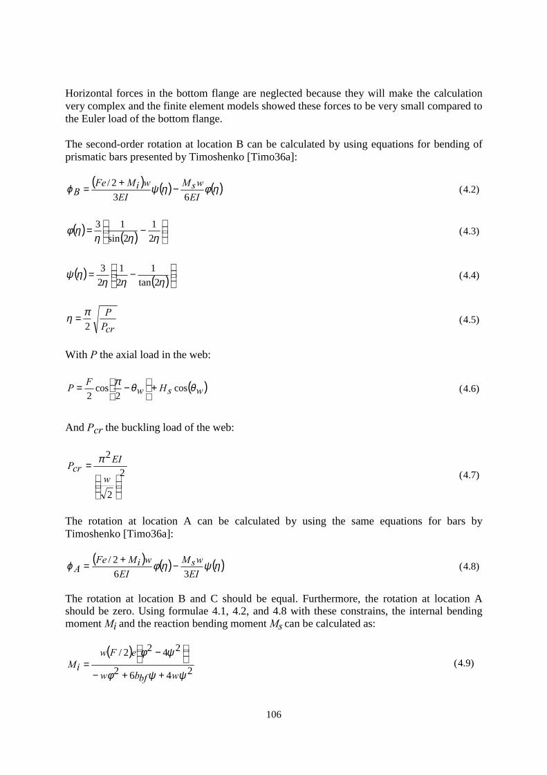
106
Horizontal forces in the bottom flange are neglected because they will make the calculationvery complex and the finite element models showed these forces to be very small compared tothe Euler load of the bottom flange.
The second-order rotation at location B can be calculated by using equations for bending ofprismatic bars presented by Timoshenko [Timo36a]:
( ) ( ) ( )ηφηψϕEI
wsMEI
wiMFeB 63
2/ −+= (4.2)
( ) ( )
−=
ηηηηφ
21
2sin13
(4.3)
( ) ( )
−=
ηηηηψ
2tan1
21
23
(4.4)
crPP
2πη = (4.5)
With P the axial load in the web:
( )wsHwFP θθπ cos
2cos
2+
−= (4.6)
And Pcr the buckling load of the web:
2
2
2
=
w
EIcrP π
(4.7)
The rotation at location A can be calculated by using the same equations for bars byTimoshenko [Timo36a]:
( ) ( ) ( )ηψηφϕEI
wsMEI
wiMFeA 36
2/ −+= (4.8)
The rotation at location B and C should be equal. Furthermore, the rotation at location Ashould be zero. Using formulae 4.1, 4.2, and 4.8 with these constrains, the internal bendingmoment Mi and the reaction bending moment Ms can be calculated as:
( )2462
2422/
ψψφ
ψφ
wbfbw
eFwiM
++−
−= (4.9)
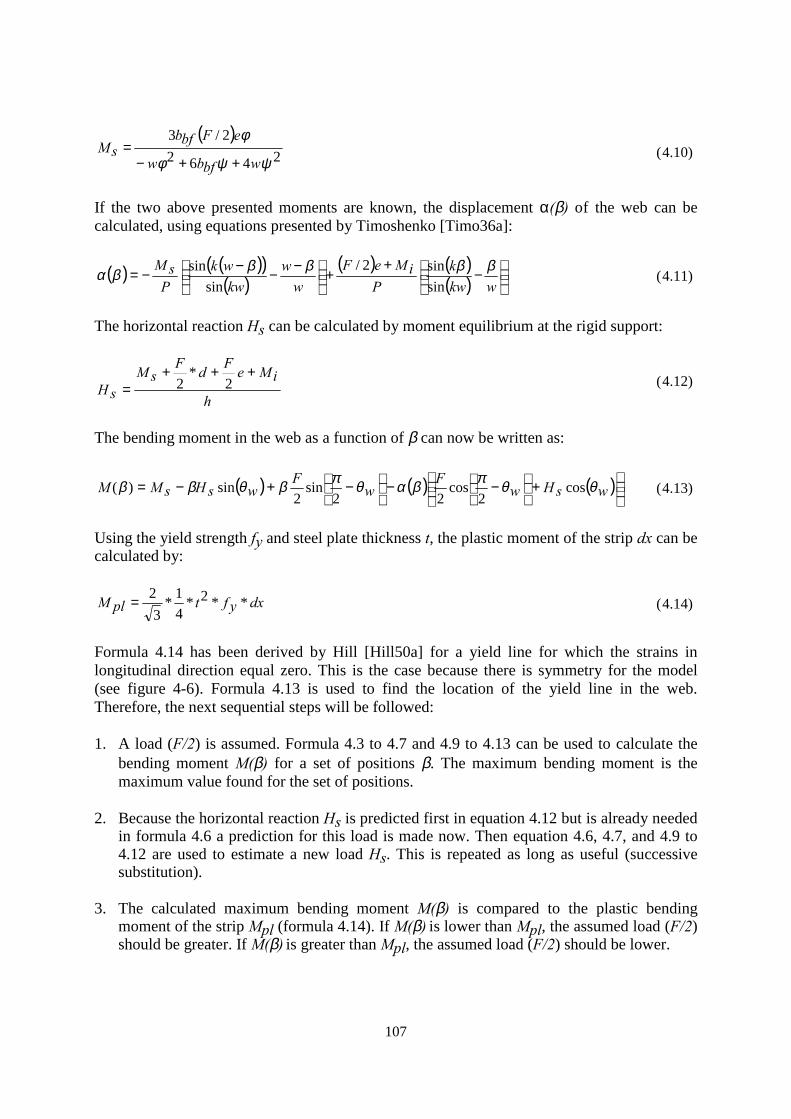
107
( )2462
2/3
ψψφ
φ
wbfbw
eFbfbsM
++−= (4.10)
If the two above presented moments are known, the displacement α(β) of the web can becalculated, using equations presented by Timoshenko [Timo36a]:
( ) ( )( )( )
( ) ( )( )
−
++
−−−−=wkw
kP
iMeFw
wkw
wkP
sM βββββαsinsin2/
sinsin
(4.11)
The horizontal reaction Hs can be calculated by moment equilibrium at the rigid support:
h
iMeFdFsM
sH+++
= 2*
2 (4.12)
The bending moment in the web as a function of β can now be written as:
( ) ( ) ( )
+
−−
−+−= wsHw
Fw
FwsHsMM θθπβαθπβθββ cos
2cos
22sin
2sin)( (4.13)
Using the yield strength fy and steel plate thickness t, the plastic moment of the strip dx can becalculated by:
dxyftplM **2*41*
32= (4.14)
Formula 4.14 has been derived by Hill [Hill50a] for a yield line for which the strains inlongitudinal direction equal zero. This is the case because there is symmetry for the model(see figure 4-6). Formula 4.13 is used to find the location of the yield line in the web.Therefore, the next sequential steps will be followed:
1. A load (F/2) is assumed. Formula 4.3 to 4.7 and 4.9 to 4.13 can be used to calculate thebending moment M(β) for a set of positions β. The maximum bending moment is themaximum value found for the set of positions.
2. Because the horizontal reaction Hs is predicted first in equation 4.12 but is already neededin formula 4.6 a prediction for this load is made now. Then equation 4.6, 4.7, and 4.9 to4.12 are used to estimate a new load Hs. This is repeated as long as useful (successivesubstitution).
3. The calculated maximum bending moment M(β) is compared to the plastic bendingmoment of the strip Mpl (formula 4.14). If M(β) is lower than Mpl, the assumed load (F/2)should be greater. If M(β) is greater than Mpl, the assumed load (F/2) should be lower.
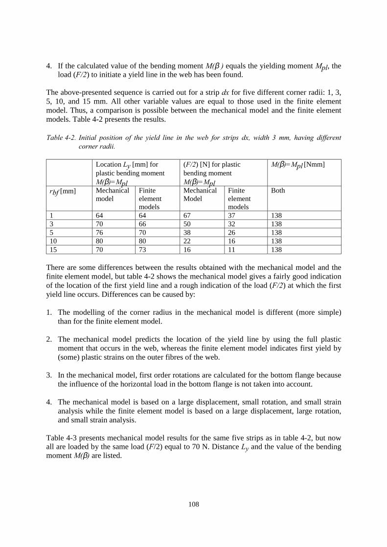
108
4. If the calculated value of the bending moment M(β ) equals the yielding moment Mpl, theload (F/2) to initiate a yield line in the web has been found.
The above-presented sequence is carried out for a strip dx for five different corner radii: 1, 3,5, 10, and 15 mm. All other variable values are equal to those used in the finite elementmodel. Thus, a comparison is possible between the mechanical model and the finite elementmodels. Table 4-2 presents the results.
Table 4-2. Initial position of the yield line in the web for strips dx, width 3 mm, having differentcorner radii.
Location Ly [mm] forplastic bending momentM(β)=Mpl
(F/2) [N] for plasticbending momentM(β)=Mpl
M(β)=Mpl [Nmm]
rbf [mm] Mechanicalmodel
Finiteelementmodels
MechanicalModel
Finiteelementmodels
Both
1 64 64 67 37 1383 70 66 50 32 1385 76 70 38 26 13810 80 80 22 16 13815 70 73 16 11 138
There are some differences between the results obtained with the mechanical model and thefinite element model, but table 4-2 shows the mechanical model gives a fairly good indicationof the location of the first yield line and a rough indication of the load (F/2) at which the firstyield line occurs. Differences can be caused by:
1. The modelling of the corner radius in the mechanical model is different (more simple)than for the finite element model.
2. The mechanical model predicts the location of the yield line by using the full plasticmoment that occurs in the web, whereas the finite element model indicates first yield by(some) plastic strains on the outer fibres of the web.
3. In the mechanical model, first order rotations are calculated for the bottom flange becausethe influence of the horizontal load in the bottom flange is not taken into account.
4. The mechanical model is based on a large displacement, small rotation, and small strainanalysis while the finite element model is based on a large displacement, large rotation,and small strain analysis.
Table 4-3 presents mechanical model results for the same five strips as in table 4-2, but nowall are loaded by the same load (F/2) equal to 70 N. Distance Ly and the value of the bendingmoment M(β) are listed.
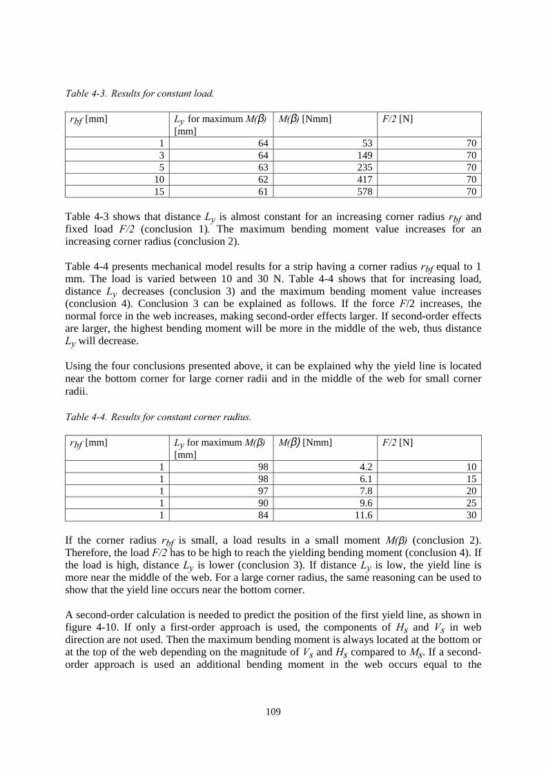
109
Table 4-3. Results for constant load.
rbf [mm] Ly for maximum M(β)[mm]
M(β) [Nmm] F/2 [N]
1 64 53 703 64 149 705 63 235 70
10 62 417 7015 61 578 70
Table 4-3 shows that distance Ly is almost constant for an increasing corner radius rbf andfixed load F/2 (conclusion 1). The maximum bending moment value increases for anincreasing corner radius (conclusion 2).
Table 4-4 presents mechanical model results for a strip having a corner radius rbf equal to 1mm. The load is varied between 10 and 30 N. Table 4-4 shows that for increasing load,distance Ly decreases (conclusion 3) and the maximum bending moment value increases(conclusion 4). Conclusion 3 can be explained as follows. If the force F/2 increases, thenormal force in the web increases, making second-order effects larger. If second-order effectsare larger, the highest bending moment will be more in the middle of the web, thus distanceLy will decrease.
Using the four conclusions presented above, it can be explained why the yield line is locatednear the bottom corner for large corner radii and in the middle of the web for small cornerradii.
Table 4-4. Results for constant corner radius.
rbf [mm] Ly for maximum M(β)[mm]
M(β) [Nmm] F/2 [N]
1 98 4.2 101 98 6.1 151 97 7.8 201 90 9.6 251 84 11.6 30
If the corner radius rbf is small, a load results in a small moment M(β) (conclusion 2).Therefore, the load F/2 has to be high to reach the yielding bending moment (conclusion 4). Ifthe load is high, distance Ly is lower (conclusion 3). If distance Ly is low, the yield line ismore near the middle of the web. For a large corner radius, the same reasoning can be used toshow that the yield line occurs near the bottom corner.
A second-order calculation is needed to predict the position of the first yield line, as shown infigure 4-10. If only a first-order approach is used, the components of Hs and Vs in webdirection are not used. Then the maximum bending moment is always located at the bottom orat the top of the web depending on the magnitude of Vs and Hs compared to Ms. If a second-order approach is used an additional bending moment in the web occurs equal to the
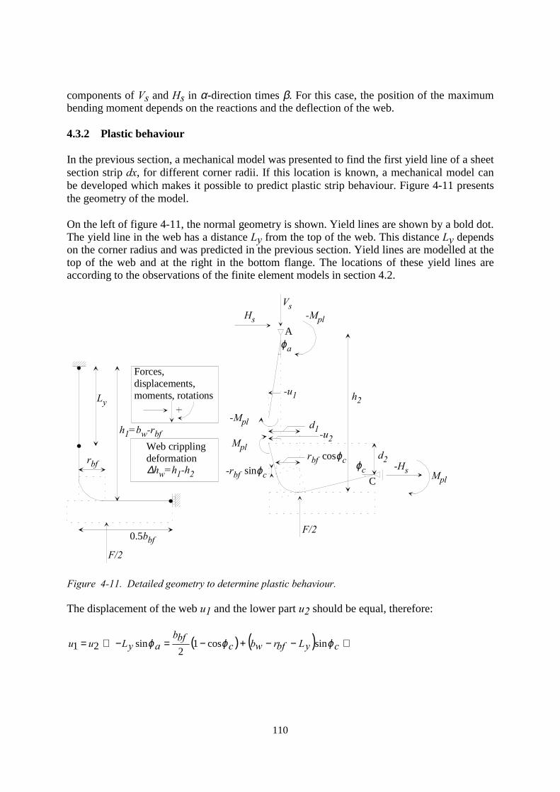
110
components of Vs and Hs in α-direction times β. For this case, the position of the maximumbending moment depends on the reactions and the deflection of the web.
4.3.2 Plastic behaviour
In the previous section, a mechanical model was presented to find the first yield line of a sheetsection strip dx, for different corner radii. If this location is known, a mechanical model canbe developed which makes it possible to predict plastic strip behaviour. Figure 4-11 presentsthe geometry of the model.
On the left of figure 4-11, the normal geometry is shown. Yield lines are shown by a bold dot.The yield line in the web has a distance Ly from the top of the web. This distance Ly dependson the corner radius and was predicted in the previous section. Yield lines are modelled at thetop of the web and at the right in the bottom flange. The locations of these yield lines areaccording to the observations of the finite element models in section 4.2.
Forces, displacements,moments, rotations
A
C
Web cripplingdeformation
F/2
0.5bbf
rbf
Ly
h1=bw-rbf
∆hw=h1-h2
F/2
-rbf sinϕc
rbf cosϕc ϕcd2
-Hs Mpl
h2
-u2d1
-u1
ϕa
-MplHs
Vs
-Mpl
Mpl
Figure 4-11. Detailed geometry to determine plastic behaviour.
The displacement of the web u1 and the lower part u2 should be equal, therefore:
( ) ( ) ⇔−−+−=−⇔= cyLbfrwbcbfb
ayLuu ϕϕϕ sincos12
sin21
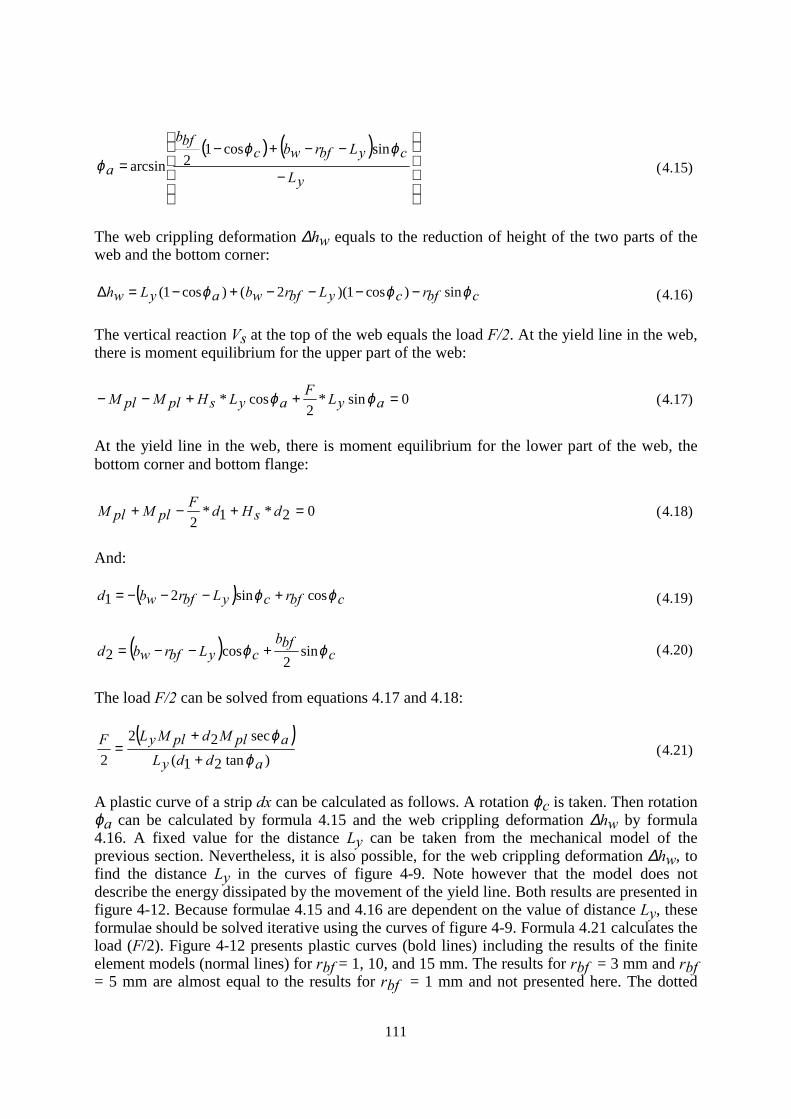
111
( ) ( )
−
−−+−=
yL
cyLbfrwbcbfb
aϕϕ
ϕsincos1
2arcsin (4.15)
The web crippling deformation ∆hw equals to the reduction of height of the two parts of theweb and the bottom corner:
cbfrcyLbfrwbayLwh ϕϕϕ sin)cos1)(2()cos1( −−−−+−=∆ (4.16)
The vertical reaction Vs at the top of the web equals the load F/2. At the yield line in the web,there is moment equilibrium for the upper part of the web:
0sin*2
cos* =++−− ayLFayLsHplMplM ϕϕ (4.17)
At the yield line in the web, there is moment equilibrium for the lower part of the web, thebottom corner and bottom flange:
02*1*2
=+−+ dsHdFplMplM (4.18)
And:
( ) cbfrcyLbfrwbd ϕϕ cossin21 +−−−= (4.19)
( ) cbfb
cyLbfrwbd ϕϕ sin2
cos2 +−−= (4.20)
The load F/2 can be solved from equations 4.17 and 4.18:
( ))tan21(
sec22
2 addyLaplMdplMyLF
ϕϕ
+
+= (4.21)
A plastic curve of a strip dx can be calculated as follows. A rotation ϕc is taken. Then rotationϕa can be calculated by formula 4.15 and the web crippling deformation ∆hw by formula4.16. A fixed value for the distance Ly can be taken from the mechanical model of theprevious section. Nevertheless, it is also possible, for the web crippling deformation ∆hw, tofind the distance Ly in the curves of figure 4-9. Note however that the model does notdescribe the energy dissipated by the movement of the yield line. Both results are presented infigure 4-12. Because formulae 4.15 and 4.16 are dependent on the value of distance Ly, theseformulae should be solved iterative using the curves of figure 4-9. Formula 4.21 calculates theload (F/2). Figure 4-12 presents plastic curves (bold lines) including the results of the finiteelement models (normal lines) for rbf = 1, 10, and 15 mm. The results for rbf = 3 mm and rbf= 5 mm are almost equal to the results for rbf = 1 mm and not presented here. The dotted
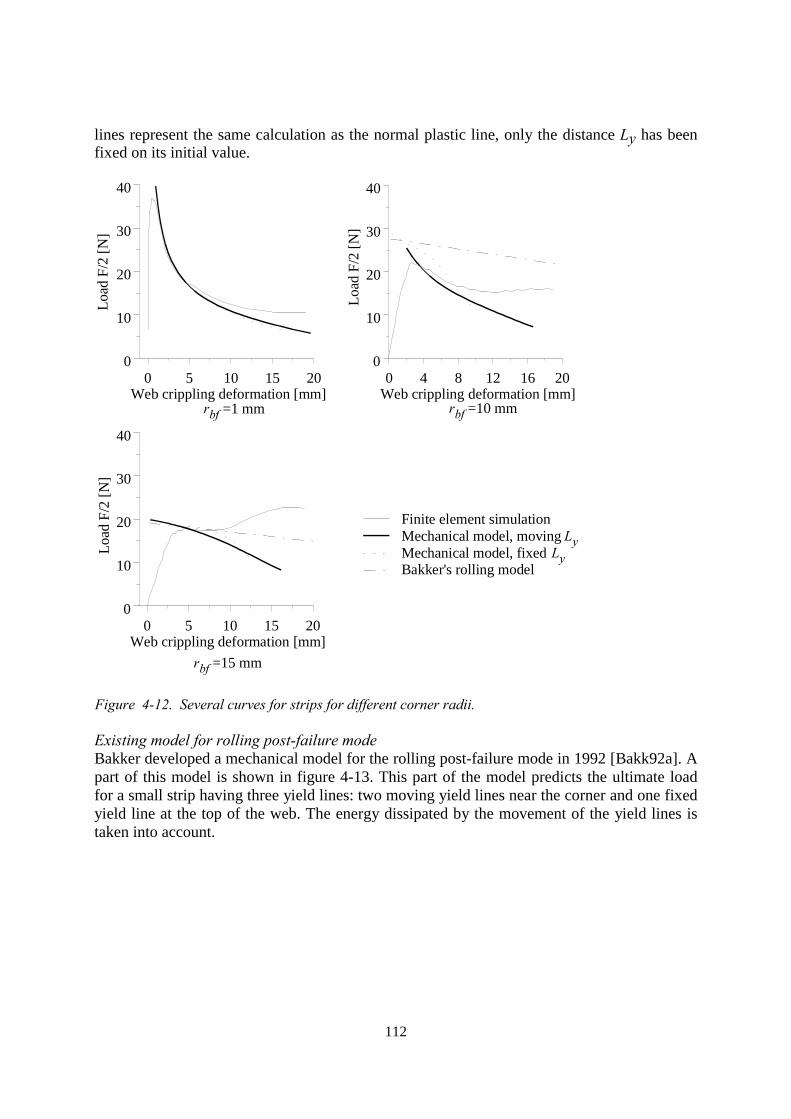
112
lines represent the same calculation as the normal plastic line, only the distance Ly has beenfixed on its initial value.
0 5 10 15 20Web crippling deformation [mm]
rbf =1 mm
0
10
20
30
40
Load
F/2
[N]
0 4 8 12 16 20Web crippling deformation [mm]
0
10
20
30
40
Load
F/2
[N]
rbf =10 mm
0 5 10 15 20Web crippling deformation [mm]
0
10
20
30
40
Load
F/2
[N]
rbf =15 mm
Finite element simulationMechanical model, movingMechanical model, fixedBakker's rolling model
Ly Ly
Figure 4-12. Several curves for strips for different corner radii.
Existing model for rolling post-failure modeBakker developed a mechanical model for the rolling post-failure mode in 1992 [Bakk92a]. Apart of this model is shown in figure 4-13. This part of the model predicts the ultimate loadfor a small strip having three yield lines: two moving yield lines near the corner and one fixedyield line at the top of the web. The energy dissipated by the movement of the yield lines istaken into account.
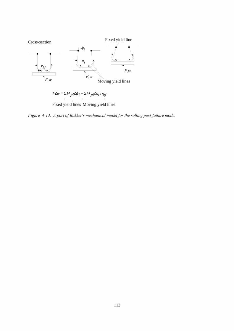
113
Cross-section
F,wF,w
F,w
Moving yield lines
Fixed yield line
Fixed yield lines Moving yield lines
rbf
ui
ϕi
bfriuplMiplMwF /δδϕδ Σ+Σ=
Figure 4-13. A part of Bakker's mechanical model for the rolling post-failure mode.
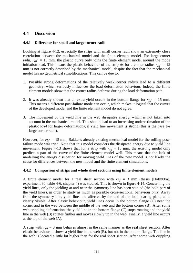
114
4.4 Discussion
4.4.1 Difference for small and large corner radii
Looking at figure 4-12, especially the strips with small corner radii show an extremely closecorrelation between the mechanical model and the finite element model. For large cornerradii, rbf = 15 mm, the plastic curve only joins the finite element model around the modeinitiation load. This means the plastic behaviour of the strip dx for a corner radius rbf = 15mm is not correctly described by the mechanical model, despite the fact that the mechanicalmodel has no geometrical simplifications. This can be due to:
1. Possible strong deformations of the relatively weak corner radius lead to a differentgeometry, which seriously influences the load deformation behaviour. Indeed, the finiteelement models show that the corner radius deforms during the load deformation path.
2. It was already shown that an extra yield occurs in the bottom flange for rbf = 15 mm.This means a different post-failure mode can occur, which makes it logical that the curvesof the developed model and the finite element model do not agree.
3. The movement of the yield line in the web dissipates energy, which is not taken intoaccount in the mechanical model. This should lead to an increasing underestimation of theplastic load for larger deformations, if yield line movement is strong (this is the case forlarge corner radii).
However, for rbf = 15 mm, Bakker's already existing mechanical model for the rolling post-failure mode was tried. Note that this model considers the dissipated energy due to yield linemovement. Figure 4-13 shows that for a strip with rbf = 15 mm, the existing model onlypredicts a part of the curve of the finite element model well. This means that the lack ofmodelling the energy dissipation for moving yield lines of the new model is not likely thecause for differences between the new model and the finite element simulations.
4.4.2 Comparison of strips and whole sheet sections using finite element models
A finite element model for a real sheet section with rbf = 3 mm (thesis [Hofm00a],experiment 30, table 4-6, chapter 4) was studied. This is shown in figure 4-14. Concerning theyield lines, only the yielding at and near the symmetry line has been studied (the bold part ofthe yield lines), in order to study as much as possible cross-sectional behaviour only. Awayfrom the symmetry line, yield lines are affected by the end of the load-bearing plate, as isclearly visible. After elastic behaviour, yield lines occur in the bottom flange (C) near thecorner and in the web between the middle of the web and the bottom corner (B). After someweb crippling deformation, the yield line in the bottom flange (C) stops rotating and the yieldline in the web (B) rotates further and moves slowly up in the web. Finally, a yield line occursat the top of the web (A).
A strip with rbf = 3 mm behaves almost in the same manner as the real sheet section. Afterelastic behaviour, it shows a yield line in the web (B), but not in the bottom flange. The line inthe web is located a little bit higher than for the real sheet section. After some web crippling
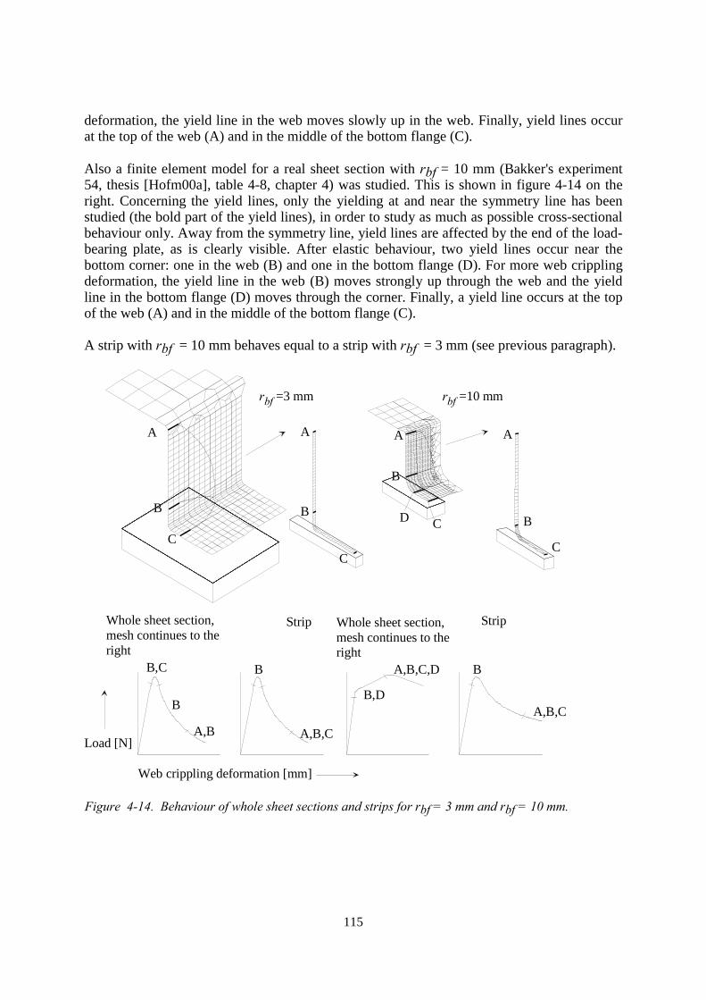
115
deformation, the yield line in the web moves slowly up in the web. Finally, yield lines occurat the top of the web (A) and in the middle of the bottom flange (C).
Also a finite element model for a real sheet section with rbf = 10 mm (Bakker's experiment54, thesis [Hofm00a], table 4-8, chapter 4) was studied. This is shown in figure 4-14 on theright. Concerning the yield lines, only the yielding at and near the symmetry line has beenstudied (the bold part of the yield lines), in order to study as much as possible cross-sectionalbehaviour only. Away from the symmetry line, yield lines are affected by the end of the load-bearing plate, as is clearly visible. After elastic behaviour, two yield lines occur near thebottom corner: one in the web (B) and one in the bottom flange (D). For more web cripplingdeformation, the yield line in the web (B) moves strongly up through the web and the yieldline in the bottom flange (D) moves through the corner. Finally, a yield line occurs at the topof the web (A) and in the middle of the bottom flange (C).
A strip with rbf = 10 mm behaves equal to a strip with rbf = 3 mm (see previous paragraph).
rbf =3 mm rbf =10 mm
Whole sheet section,mesh continues to theright
Strip Whole sheet section,mesh continues to theright
Strip
A
B
C
A
B
C
A
B
C
A
B
CD
B,C
B
A,B
B
A,B,C
B
A,B,CB,D
A,B,C,D
Web crippling deformation [mm]
Load [N]
Figure 4-14. Behaviour of whole sheet sections and strips for rbf = 3 mm and rbf = 10 mm.
116
4.5 Conclusions
For three-point bending tests of sheet sections, the location of the first yield line in the webdepends on the post-failure mode. For a rolling post-failure mode, the first yield line occurs inthe web near the bottom corner and for a yield arc post-failure mode, the first yield line occursin the lower middle of the web. The mechanical model for a strip dx of the sheet section,explains these different yield line locations. Only one mechanical model was used to showthis for both post-failure modes. A second-order calculation is necessary to predict thelocation of the first yield line in the web. The mechanical model can be used to predict theposition of the yield line in the web, for both strips and whole sheet sections.
For the finite element models of the strips dx, for intermediate corner radii, behaviour occursthat is a transition between the behaviour for large corner radii and small corner radii. This isnot only seen for the load deformation behaviour, but also for the location and movement ofthe first yield line. As a conclusion, the strips dx do not fail by two completely different post-failure modes. This was also observed for three-point bending tests [Bakk92a], wheresometimes a failure occurred which was a mixture of the yield arc and rolling post-failuremodes.
A mechanical model has been developed to find the plastic curves for comparison with thefinite element models of the strips dx. Only one model was used. The model predicts theplastic curve of the strips well for rbf =1, 3, 5, and 10 mm. For the large corner radius rbf =15 mm only a small part of the curve is covered.
For small corner radii, the behaviour of a strip of a sheet section's cross-section isqualitatively similar to the behaviour of a real sheet section in a three-point bending test. Forrbf = 10 mm, this is not the case (comparisons made based on finite element analysis). Thus,strip behaviour cannot be used to explain whole sheet section behaviour.
For a large corner radius, rbf = 15 mm, an already existing mechanical model for the rollingpost-failure mode predicts the first part of the plastic curve well. The finite element modelshows that for a strip with rbf = 15 mm, two yield lines occur near the bottom corner. Thismakes it possible that for a strip with rbf = 15 mm, indeed a rolling post-failure mode occurs.This needs further investigation.
Further research can be focussed on two items. First, boundary conditions of the strips can bestudied for large corner radii. In this way, an explanation can be found for the differentbehaviour between strips and three-point bending tests. Secondly, for small corner radii, it canbe investigated how the strip behaviour can be translated into behaviour of three-pointbending tests.

117
5 Appendix Turbo Pascal programs
5.1 Program for Eurocode3 predictions
VAR
{Input/output}bbffl,b1,b2:Real;htest,out:Text;counter:Integer;testno:Real;btf2:Real;
{UFF Format}typee,ref,btf,rtf,bw,bbf,rbf,tw,Lspan,Llb,t,fy,Ftest,Fimec:Real;
{Section}E:Real;
{Sheeting/three point bending tests}sh,ctp:Real;
{5.4.3 Effects of shear lag}sla,slb,slc,sld,beta2,delta,neta:Real;
{5.4.1 Calculating Mu, top flange yields first}error2:Real;
{5.4.1 Calculation Mu, bottom flange yields first}Cy,sc,la1,la2:Real;
{5.9.3 Web crippling strength}error1,lafu,alfa,Rw:Real;
{5.11 Combined bending and web crippling}fac1,fac2,eta,F:Real;
rholx,bfyields,ftf,fbf,yc,Mu,Mn,Cy2:Real;
FUNCTION tan(x:Real):Real;BEGINtan:=sin(x)/cos(x);END;
FUNCTION power(x,y:Real):Real;{calculates x to the power y}BEGINPower:=EXP(y*LN(x));END;

118
PROCEDURE EFFECTIVE_WIDTH;
{Calculates ultimate bending moment Mn if only outer fibre} {tension or compression flange yields}
VAR
sest,s,ebf,etf,bbfp,ksig,lap,be3,rho:Real; e1,e2,f1,f2,psi,bwp,be1,be2,sest2,s22,sub1,sub2,sub3,sub4:Real; a1,s1,a2,s2,a34,s34,a6,s6,a7,s7,a8,s8,I,w:Real;
BEGIN
sest:=0.5*bw*sin(tw); s:=10000;
WHILE abs(s-sest)>0.001 DO
BEGIN
s:=sest;
IF (bfyields=1) THEN BEGIN ebf:=fy/E; etf:=ebf*(bw*sin(tw)-(s-0.5*t))/(s-0.5*t); END;
IF (bfyields=0) THEN BEGIN etf:=fy/E; ebf:=etf*(s-0.5*t)/(bw*sin(tw)-(s-0.5*t)); END;
fbf:=ebf*E; ftf:=etf*E;
{4.2 Plane elements without stiffeners}
bbfp:=bbf-2*rbf*(tan(tw/2)-sin(tw/2)); ksig:=4; lap:=1.052*(bbfp/t)*sqrt(fy/(E*ksig)); lap:=lap*sqrt(fbf/fy); IF (lap<=0.673) THEN BEGIN rho:=rholx*1; END; IF (lap>0.673) THEN BEGIN rho:=rholx*(1-0.22/lap)/lap; END; be3:=0.5*rho*bbfp;
e1:=ebf*(s-0.5*t-rbf*tan(0.5*tw)*sin(tw))/(s-0.5*t); e2:=etf*((bw*sin(tw)-(s-0.5*t))-rtf*tan(0.5*tw)*sin(tw)); e2:=e2/(bw*sin(tw)-(s-0.5*t)); f1:=e1*E;
119
f2:=-e2*E; psi:=f2/f1; bwp:=bw-(rbf+rtf)*(tan(tw/2)-sin(tw/2)); ksig:=7.81-6.29*psi+9.78*sqr(psi); IF (psi<-1) AND (psi>-3) THEN BEGIN ksig:=5.98*sqr(1-psi); END; lap:=1.052*(bwp/t)*sqrt(fy/(E*ksig)); lap:=lap*sqrt(f1/fy); IF (lap<=0.673) THEN BEGIN rho:=1; END; IF (lap>0.673) THEN BEGIN rho:=(1-0.22/lap)/lap; END; be1:=0.4*rho*bwp; be2:=0.6*rho*bwp;
sest2:=s; s22:=10000;
WHILE abs(sest2-s22)>0.001 DO
BEGIN
s22:=sest2;
sub1:=rtf*tan(0.5*tw); sub2:=rtf*tan(0.5*tw)*sin(tw); sub3:=rbf*tan(0.5*tw); sub4:=rbf*tan(0.5*tw)*sin(tw);
a1:=0.5*btf-sub1; a1:=a1*t; s1:=bw*sin(tw)+0.5*t;
a2:=t*rtf*tw; s2:=bw*sin(tw)+0.5*t-rtf+(rtf*sin(tw)/tw);
a34:=bw-(s22-0.5*t)/sin(tw)-sub1+be2; a34:=a34*t; s34:=bw*sin(tw)+0.5*t-(sub1+(a34/t)*0.5)*sin(tw);
a6:=be1-rbf*(sin(tw/2)); a6:=a6*t; s6:=(0.5*be1+rbf*(tan(tw/2)-sin(tw/2)))*sin(tw)+0.5*t;
a7:=t*rbf*tw; s7:=rbf+0.5*t-(rbf*sin(tw)/tw);
a8:=be3-rbf*(sin(tw/2)); a8:=a8*t; s8:=0.5*t;
sest2:=(a1*s1+a2*s2+a34*s34+a6*s6+a7*s7+a8*s8); sest2:=sest2/(a1+a2+a34+a6+a7+a8); END;

120
sest:=s22;
{----------------------------------------------------------------}
END;
{MOMENT OF INERTIA----------------------------------------------------}
I:=a1*sqr(s1)+a2*sqr(s2)+a34*sqr(s34)+a6*sqr(s6)+a7*sqr(s7)+a8*sqr(s8); I:=I-(a1+a2+a34+a6+a7+a8)*sqr(s); I:=I*2;
{---------------------------------------------------------------------}
W:=I/s; IF bfyields=0 THEN BEGIN W:=I/(bw*sin(tw)-s); END; Mn:=W*fy; END;
PROCEDURE INELASTIC_CAP;
{Calculates ultimate bending moment for plastic compression and, if} {applicable, tension zone}
{Reck, Pekoz, and Winter do not take into account corner geometry} {and only use fully effective webs} {Fully effective webs can be used because: }
{Situation 1, bottom flange (tension) yields} {bwp/t<2.22*sqrt(E/fy) (is requested by code), than psi=-1, ksig=23.9} {lap=0.48, rho=1, be1=0.4bwp, be2=0.6bwp, be1 and be2 together} {more than 0.5bwp, thus web fully effective}
{Situation 2, bottom flange (tension) does not yield} {most extreme situation: no tension at all in web: psi=0, k=7.81} {bwp/t<1.11*sqrt(E/fy), lap=0.42, rho=1, be1=(2/5)bwp, be2=bwp-be1} {be1 and be2 equal to bwp thus web fully effective}
VAR {Procedure inelastic_cap} bbfp,ksig,lap,rho,be3,bc,bt,d,la1,la2,ycest,sc,Cy:Real; yp,yt,ycp,ytp,eqa,eqb,eqc,yc1,yc2,ft:Real;
BEGIN
bbfp:=bbf-2*rbf*(tan(tw/2)-sin(tw/2)); ksig:=4; lap:=1.052*(bbfp/t)*sqrt(fy/(E*ksig)); IF (lap<=0.673) THEN BEGIN rho:=rholx*1; END; IF (lap>0.673) THEN BEGIN rho:=rholx*(1-0.22/lap)/lap; END; be3:=0.5*rho*bbfp;
121
bc:=2*be3+2*rbf*(tan(tw/2)-sin(tw/2)); bt:=btf; d:=bw*sin(tw);
{5.4.2 Partially plastic resistance}
la1:=1.11*sqrt(E/fy); la2:=1.29*sqrt(E/fy);
Cy:=3-((bc/t)*sqrt(fy/E)-1.11)/0.09; IF (bc/t) <= la1 THEN BEGIN Cy:=3; END; IF (bc/t) >= la2 THEN BEGIN Cy:=1; END;
{Paper Reck, Pekoz, Winter. J. of the Struc. Div. Nov, 1975} {with an self-made extension for inclined webs}
yc:=0.25*(bt*sin(tw)-bc*sin(tw)+2*d); yp:=yc/Cy; yt:=d-yc; ycp:=yc-yp; ytp:=yt-yp;
Mu:=fy*t*bc*yc; Mu:=Mu+2*fy*t*(ycp/sin(tw))*(yc-0.5*ycp); Mu:=Mu+2*0.5*fy*t*(yp/sin(tw))*((2/3)*yp);
Mu:=Mu+2*0.5*fy*t*(yp/sin(tw))*((2/3)*yp); Mu:=Mu+2*fy*t*(ytp/sin(tw))*(yt-0.5*ytp); Mu:=Mu+fy*t*bt*yt;
IF (yp>yt) AND (Cy>1) THEN
BEGIN eqa:=(2/sin(tw))-(1/(Cy*sin(tw)))-(Cy/sin(tw)); eqb:=bc+(2*Cy*d/sin(tw))+Cy*bt; eqc:=-Cy*sqr(d)/sin(tw)-Cy*bt*d; yc1:=(-eqb+sqrt(sqr(eqb)-4*eqa*eqc))/(2*eqa); yc2:=(-eqb-sqrt(sqr(eqb)-4*eqa*eqc))/(2*eqa);
{yc1 gives normal values, yc2 > 100 * h}
yc:=yc1; yp:=yc/Cy; yt:=d-yc; ycp:=yc-yp; ft:=fy*Cy*yt/yc;
Mu:=fy*t*bc*yc; Mu:=Mu+2*fy*t*(ycp/sin(tw))*(yc-0.5*ycp); Mu:=Mu+2*0.5*fy*t*(yp/sin(tw))*((2/3)*yp);

122
Mu:=Mu+2*0.5*ft*t*(yt/sin(tw))*((2/3)*yt); Mu:=Mu+ft*t*bt*yt; END;
END;
BEGIN {Program}
ASSIGN(htest,'tswt3.prn');ASSIGN(out,'tswteta.dat');REWRITE(out);
FOR counter:=1 to 196 DO
BEGIN
writeln('Counter: ',counter);
{Input----------------------------------------------------------------}
RESET(htest); READ(htest,testno);
WHILE testno<>counter DO BEGIN READLN(htest); READ(htest,testno); END;
READ(htest,ref,typee,btf,rtf,bw,bbf,rbf,tw,Lspan,Llb,t,fy,Ftest,Fimec);
sh:=1; {1:sheeting, 2:hat sections} ctp:=2; {1:continuous, 2:three point bending test}
tw:=tw/57.29577951; E:=210000; CLOSE(htest);
{3.1.2 Average yield strength (strength increase cold work)-----------}
{Not used: 3.1.2(5):no fully effective flanges------------------------}
{---------------------------------------------------------------------}
{Flange curling-------------------------------------------------------}
{No clauses in Eurocode about flange curling--------------------------}
{---------------------------------------------------------------------}
123
{5.4.3 Effects of shear lag-------------------------------------------}
IF ctp=1 THEN BEGIN sla:=6; slb:=1.6; slc:=1.155; sld:=7.76; END;
IF ctp=2 THEN BEGIN sla:=4; slb:=3.2; slc:=1.115; sld:=5.74; END;
{top flange under tension}
IF ((0.5*btf)/Lspan) > (1/20) THEN BEGIN beta2:=1+sla*(0.5*btf/Lspan)+slb*sqr(0.5*btf/Lspan); beta2:=1/beta2; END;
IF ((0.5*btf)/Lspan) < (1/50) THEN BEGIN beta2:=1.0; END;
IF (((0.5*btf)/Lspan) <= (1/20)) AND (((0.5*btf)/Lspan) >= (1/50)) THEN BEGIN beta2:=slc-sld*(0.5*btf/Lspan); END;
btf:=beta2*btf;
{bottom flange under compression}
IF ((0.5*bbf)/Lspan) > (1/20) THEN BEGIN beta2:=1+sla*(0.5*bbf/Lspan)+slb*sqr(0.5*bbf/Lspan); beta2:=1/beta2; END;
IF ((0.5*bbf)/Lspan < (1/50)) THEN BEGIN beta2:=1.0; END;
124
IF (((0.5*bbf)/Lspan) <= (1/20)) AND (((0.5*bbf)/Lspan) >= (1/50)) THEN BEGIN beta2:=slc-sld*(0.5*bbf/Lspan); END;
delta:=(bbf/t)*sqrt(fy/E); IF delta <= 1 THEN BEGIN delta:=1; END; neta:=(0.5*bbf/Lspan)/delta; rholx:=power(beta2,neta);
{---------------------------------------------------------------------}
{5.4.1 Calculating Mu-------------------------------------------------}
bfyields:=1; EFFECTIVE_WIDTH;
IF ftf >= fy THEN BEGIN bfyields:=0; EFFECTIVE_WIDTH; END;
INELASTIC_CAP;
error2:=0; IF (tw<(60/57.29577951)) THEN BEGIN error2:=1; END; IF ((((yc/sin(tw))-rtf*tan(0.5*tw))/t)>(1.11*sqrt(E/fy))) THEN BEGIN error2:=1; END;
IF error2=0 THEN
BEGIN Mn:=Mu; END;
{5.9.3 Web crippling strength-----------------------------------------}
error1:=0; IF ((rbf-0.5*t)/t) > 10 THEN BEGIN error1:=1; END; IF (bw*sin(tw)/t) > 200*sin(tw) THEN BEGIN error1:=1; END; IF tw < (45/57.29577951) THEN BEGIN error1:=1; END; IF tw > (90/57.29577951) THEN BEGIN error1:=1; END; IF error1=1 THEN BEGIN writeln('WARNING:');
125
writeln('SECTION PROPERTIES ARE NOT IN VALID RANGE'); writeln('AS SPECIFIED BY THE EUROCODE FOR Rw CALCULATION'); END;
IF (Lspan-Llb)/2 <= 1.5*bw*sin(tw) THEN BEGIN lafu:=10; IF sh=1 THEN BEGIN alfa:=0.075; END; IF sh=2 THEN BEGIN alfa:=0.057; END; END;
IF (Lspan-Llb)/2 > 1.5*bw*sin(tw) THEN BEGIN lafu:=Llb; IF sh=1 THEN BEGIN alfa:=0.15; END; IF sh=2 THEN BEGIN alfa:=0.115; END; END;
Rw:=alfa*sqr(t)*sqrt(fy*E)*(1-0.1*sqrt((rbf-0.5*t)/t)); Rw:=2*Rw*(0.5+sqrt(0.02*lafu/t))*(2.4+sqr(tw*57.29577951/90));
{---------------------------------------------------------------------}
{5.11 Combined bending and web crippling strength---------------------}
fac1:=-1; fac2:=+1.25; eta:=0.25*(Rw/Mn)*(Lspan-Llb);
F:=(fac2*Rw/(eta-fac1)); IF (eta<((fac1+fac2)/1)) THEN BEGIN F:=Rw; END; IF (eta>(fac1/(1-fac2))) THEN BEGIN F:=Rw/eta; END;
{---------------------------------------------------------------------}
IF error1=0 THEN BEGIN writeln(out,counter,chr(9),eta,chr(9),F); END; IF error1=1 THEN BEGIN writeln(out,counter,chr(9),'0',chr(9),'0'); END;
END;
CLOSE(out);
END.

126
5.2 Program for ultimate failure mechanical model
var
out:Text;teller:Integer;testno:Real;
{UFF-format}ref,typee,btf,rtf,bw,bbf,rbf,tw,Lspan,Llb,t,fy,Ftest,Fimec:Real;
F,Fmin,Fmax:Real;KK1,KK2,alfa,I,I2,k,k2,e,beta,dhw,dhw2:Real;{2}Rh,dhcs,dhcs2:Real;{3}Fbf:Real;{4}w0max,w0min,pa:Real;marker:Real;
M,ee,mu,pi,b,L,w0,y0,x,z:Real;be,la,w,y,D,c1,c2:Real;p,p2,sx,sz,txz,sxm,sx2,szm,svm,svm2:Real;
harpje,Fcr:Real;
hn,zpnov,Inov,Wnov,Snov:Real;
function power(x,y:Real):Real;{calculates x to the power y}begin power:=exp(y*ln(x));end;
function cosh(x:Real):Real;{calculates the hyperbolic cosine for x}begin cosh:=0.5*(exp(x)+exp(-x));end;
function sinh(x:Real):Real;{calculates the hyperbolic sine for x}begin sinh:=0.5*(-exp(-x)+exp(x));end;
function TAN(x:Real):Real;begin TAN:=SIN(x)/COS(x);end;

127
function coth(x:Real):Real;{calculates the hyperbolic cot for x}begin coth:=cosh(x)/sinh(x);end;
begin
assign(out,'tswt3a.dat');REWRITE(out);
ASSIGN(input,'tswt3.prn');
FOR teller:= 1 TO 196 DO BEGIN {FOR for all tested sections} RESET(input); READ(input,testno); while teller<>testno DO begin READLN(input); READ(input,testno); end; READ(input,ref,typee,btf,rtf,bw,bbf,rbf,tw,Lspan,Llb,t,fy,Ftest,Fimec); CLOSE(input); tw:=tw/57.29577951;
{initialisation}writeln(teller);writeln('rbf ',rbf);writeln('bw ',bw);writeln('btf ',btf);writeln('tw ',tw*57.29577951);writeln('Lspan ',Lspan);writeln('Llb ',Llb);writeln('fy ',fy);
e:=210000;
{0) assuming load}
Fmin:=0;Fmax:=4*Ftest;svm:=0;
WHILE abs(svm-fy) > 0.1 DO
begin
F:=(Fmin+Fmax)/2;
{1) calculating dhw}

128
{using beam on elastic foundation model}
alfa:=0.118*power(rbf,0.89);
I:=((t*alfa*bw)/2)*sqr((bbf*alfa*bw*sin(tw)+t*bbf)/(bbf+2*alfa*bw));I:=I+bbf*t*sqr((alfa*alfa*bw*bw*sin(tw)+alfa*bw*t)/(bbf+2*alfa*bw));I2:=(alfa*alfa+bw*bw+t*t)/12;I2:=I2-(cos(2*tw)*(alfa*alfa*bw*bw-t*t))/12;I2:=I2+(t*alfa*bw*sin(2*tw))/2;I2:=I2*t*alfa*bw;I:=((bbf*t*t*t)/12)+I2+I;
k:=bw*(bbf-(4/3)*rbf*sin(tw))+rbf*sin(tw)*(bbf-(3/2)*rbf*sin(tw));k:=(k/(e*(3*bbf+2*bw)))*rbf*rbf*sin(tw)*sin(tw)*(12/(t*t*t));k2:=bw*cos(tw)*((2/3)*bw+bbf)+rbf*bbf*sin(tw)-rbf*rbf*sin(tw)*sin(tw);k2:=(k2/(bbf+(2/3)*bw))*((cos(tw))/(e*t));k:=k+k2+((bw*sin(tw)*sin(tw))/(e*t));k:=1/k;
beta:=k/(4*e*I);beta:=power(beta,0.25);
dhw:=exp(-beta*0.5*(Lspan-Llb))*(cos(beta*0.5*(Lspan-Llb))-sin(beta*0.5*(Lspan-Llb)));dhw:=dhw+exp(-beta*0.5*(Lspan+Llb))*(cos(beta*0.5*(Lspan+Llb))-sin(beta*0.5*(Lspan+Llb)));dhw2:=exp(-beta*(Lspan-Llb))*sin(beta*(Lspan-Llb));dhw2:=dhw2+exp(-beta*(Lspan+Llb))*sin(beta*(Lspan+Llb));dhw:=dhw*dhw2;dhw:=1+exp(-beta*Llb)*(cos(beta*Llb)+sin(beta*Llb))-dhw;dhw:=dhw*((F*beta)/(4*k));
{2) calculating cross-section deformation dhcs}
rh:=(2/3)*bw*bw*cos(tw)+rbf*sin(tw)*bbf+bbf*bw*cos(tw)-rbf*rbf+sin(tw)*sin(tw);rh:=rh/((1/2)*bbf+(1/3)*bw);rh:=(rh*k*dhw)/(4*bw*sin(tw));
dhcs:=((k*dhw)/(2))*(bw*cos(tw)+rbf*sin(tw));dhcs:=dhcs-rh*(bw*sin(tw)-dhw);dhcs:=dhcs/(2*((1/12)*1*t*t*t)*e);dhcs:=dhw+abs(dhcs*sqr((bbf/2)-rbf*sin(tw)));
hn:=bw*sin(tw); zpnov:=(2*hn*t*0.5*hn)+(bbf*t*hn); zpnov:=zpnov/(t*(btf+hn+hn+bbf)); Inov:=(1/12)*power(t,3)*btf+zpnov*zpnov*t*btf; Inov:=Inov+2*(power(hn,3)*t*(1/12)+sqr((hn/2)-zpnov)*hn*t); Inov:=Inov+power(t,3)*bbf*(1/12)+sqr(hn-zpnov)*bbf*t; Wnov:=Inov/(hn-zpnov); Snov:=(F*(Lspan-Llb)/4)/Wnov; Fbf:=Snov*bbf*t;
129
{4) find wo for this situation}
y0:=sqrt(2)*(dhcs-dhw); w0min:=0; w0max:=bbf/10;
{Marquerre equations .........................................................}
e:=210000; {N/mm2, Youngs modulus}mu:=0.3; {1, Poissons ratio}pi:=3.14159265; {1}
b:=bbf-2*rbf*tan(0.5*tw); {mm, steel plate width}L:=b; {mm, steel plate length}
x:=b/2; {mm, position in x-direction}z:=0*b; {mm, position in z-direction}
{calculating w, y, be, la, and D, some variables needed}
be:=pi/b;la:=pi/L;pa:=1;
WHILE abs(Fbf-pa*e*t*b)>0.01 DO
begin
w0:=(w0min+w0max)/2; w:=w0*cos(be*x)*cos(la*z);
y:=y0*cos(be*x)*cos(la*z);D:=(e*t*t*t)/(12*(1-mu*mu));
KK1:=0; KK2:=1;
{calculating c1 and c2, constants needed to predict stresses}
c1:=b*sinh(la*b);c1:=c1-b*cosh(la*b)*coth(la*b);c1:=c1-(1/la)*cosh(la*b);c1:=c1*32*la*la;c1:=(-be*be*(b*coth(la*b)+(1/la)))/c1;c1:=c1*w0*(w0+2*y0);
c2:=b*sinh(la*b);c2:=c2-b*cosh(la*b)*coth(la*b);c2:=c2-(1/la)*cosh(la*b);c2:=c2*16*la*la;c2:=(be*be)/c2;c2:=c2*w0*(w0+2*y0);
130
{Finding p, average axial compressive stress in z direction}
p:=(1/2)*(((sqr(la)-sqr(be))/(sqr(sqr(la)+sqr(be))))-(1/(sqr(la))))*sinh(la*b);p:=p+((la*b)/2)*((1/(sqr(la)))-((1)/(sqr(la)+sqr(be))))*cosh(la*b);p:=p*(1/8)*L*sqr(la)*c2*KK2*(w0+y0)*(sqr(be)-sqr(la));p:=p+(1/8)*L*sqr(be)*c1*KK2*la*(w0+y0)*sinh(la*b);
p2:=((be*b)/2)*cosh(la*b);p2:=p2-((be*la)/(sqr(la)+sqr(be)))*sinh(la*b);p2:=p2*(w0+y0);p2:=p2*((L*c2*KK2*la*la*la*be)/(4*(sqr(la)+sqr(be))));
p:=p+p2;p:=p/((b*L)/(32));p:=p-(1/8)*w0*(w0+y0)*(w0+2*y0)*(la*la*la*la+be*be*be*be*(2*KK1+1));p:=p-2*((d*w0)/(e*t))*sqr(sqr(la)+sqr(be));p:=p/(2*(w0+y0)*(sqr(la)+mu*be*be*KK1));
pa:=abs(p);
if (pa*e*t*b)<Fbf then w0min:=w0; if (pa*e*t*b)>Fbf then w0max:=w0; if (pa*e*t*b)=Fbf then w0:=w0;
end;
{Calculating the membrane stresses sz, sx, and txz}
sz:=4*sqr(la)*x*sinh(2*la*x)+4*la*cosh(2*la*x);sz:=sz*c2;sz:=sz+4*c1*sqr(la)*cosh(2*la*x);sz:=sz*cos(2*la*z)*KK2;sz:=sz+w0*(w0+2*y0)*((sqr(la))/(8))*cos(2*be*x);sz:=sz+p;sz:=sz*e;
sx:=c1*cosh(2*la*x);sx:=sx2+c2*x*sinh(2*la*x);sx:=sx2*-4*sqr(la)*cos(2*la*z)*KK2;
sx:=sx2+w0*(w0+2*y0)*((sqr(be))/(8))*(KK1+cos(2*la*z)); sx:=sx2+mu*KK1*p;
sx:=sx2*e;
txz:=2*la*x*cosh(2*la*x)+sinh(2*la*x);txz:=txz*c2;txz:=txz+2*la*c1*sinh(2*la*x);txz:=txz*2*la*sin(2*la*z)*KK2;txz:=txz*e;
{Calculating the bending moment stresses szm and sxm}
szm:=E*w0*t*(la*la+mu*be*be);

131
szm:=szm/(2*(1-mu*mu));szm:=szm*cos(la*z)*cos(be*x);
sxm:=E*w0*t*(be*be+mu*la*la);sxm:=sxm/(2*(1-mu*mu));sxm:=sxm*cos(la*z)*cos(be*x);
{Calculating the Von Mises stress at (x,z)}
svm:=sqrt((sx+sxm)*(sx+sxm)+(sz+szm)*(sz+szm)-(sx+sxm)*(sz+szm)+3*txz*txz);svm2:=sqrt((sx-sxm)*(sx-sxm)+(sz-szm)*(sz-szm)-(sx-sxm)*(sz-szm)+3*txz*txz);
if svm >= svm2 thenbeginsvm:=svm;end;
if svm < svm2 thenbeginsvm:=svm2;end;
{Marquerre equations..........................................................}
if svm >= fy then begin Fmax:=F; end;
if svm < fy then begin Fmin:=F; end;
end;
Fcr:=12*(1-sqr(0.3))*sqr(b);Fcr:=b*t*4*210000*sqr(pi)*sqr(t)/Fcr;IF Fcr<Fbf THENBEGINharpje:=1;END;writeln(out,teller,chr(9),F);
end;
close(out);
end.

132
5.3 Program for post-failure mechanical model MA1
var
{Input and output variables}out:Text;teller:Integer;yax6tab:Text;testno,destestno:String[4];woord1,woord2:String;
{Section variables}hw,btf,bw,bbf,th,rbf,rtf:Real;k,E,Llb,L,Lw,Lbf,t,fy:Real;typee,Ltf,A,I,ref,Ftest,Fimec:Real;
{Calculation variables}dhw,Fp,AA,BB,CC,s,c,pi,alfa,beta:Real;Lwtry,aaaa,bbbb,cccc,fi2,wtf,ddhw_dfi,dfi_ddhw,lfb:Real;
{Finding Lw}mpl,d,w,h,sigma1,sigma2,sigma,upsilon,xmax,Mmax,M,F,Mi,Mr,Hr:Real;Fmin,Fmax,Pcr,P,u,kk,fi,psi,Hrest:Real;tau:Integer;
function Sec(x:Real):Real;begin Sec:=1/Cos(x);end;
function Tan(x:Real):Real;begin Tan:=Sin(x)/Cos(x);end;
function Cot(x:Real):Real;begin Cot:=Cos(x)/Sin(x);end;
function ArcSin(x:Real):Real;{-90<ArcSin(x)<90}var sinx,cosx:Real;begin sinx:=x; cosx:=SQRT(1-SQR(sinx)); ArcSin:=ArcTan(sinx/cosx);end;
function ArcCos(x:Real):Real;{0<ArcCos(x)<180}

133
var sinx,cosx:Real;begin cosx:=x; sinx:=SQRT(1-SQR(cosx)); if x=0 then ArcCos:=pi/2; if x>0 then ArcCos:=ArcTan(sinx/cosx); if x<0 then ArcCos:=ArcTan(sinx/cosx)+pi;end;
function Power(x,y:Real):Real;{calculates x to the power y}begin Power:=EXP(y*LN(x));end;BEGIN
ASSIGN(out,'uff234b.dat');REWRITE(out);
FOR teller:= 1 TO 58 DOBEGIN {FOR for all tested sections}str(teller,woord1);woord2:=' ';destestno:=woord1+woord2;ASSIGN(yax6tab,'uff234.uff');RESET(yax6tab);READ(yax6tab,testno);while testno<>destestno dobeginREADLN(yax6tab);READ(yax6tab,testno);end;READ(yax6tab,ref,typee,btf,rtf,bw,bbf,rbf,th,L,Llb,t,fy,Ftest,Fimec);th:=th/57.29577951;CLOSE(yax6tab);pi:=3.141592654;E:=210000;s:=Sin(th);c:=Cos(th);hw:=bw*s;
{FINDING LW -------------------------------------------------------------------}
I:=(1/12)*3*power(t,3);w:=bw-rbf*tan(th/2);
Pcr:=sqr(pi)*E*I/sqr(0.7*w);mpl:=(2/sqrt(3))*3*0.25*1.155*fy*sqr(t);Mmax:=0;Fmin:=0.1;Fmax:=2.2*Pcr;

134
IF (ref=1) OR (ref=22) OR (ref=26) THENBEGINFmax:=3*Pcr;END;
IF (ref=27) OR (ref=28) OR (ref=29) THENBEGINFmax:=2.5*Pcr;END;
WHILE abs(abs(Mmax)-mpl) > 1 DO
BEGIN
F:=(Fmin+Fmax)/2;Mmax:=0;
FOR tau:= 1 TO round(w-rbf*tan(th/2)) DO
BEGIN
d:=w*cos(th); h:=w*sin(th);
Hr:=1; Hrest:=0;
WHILE abs(Hrest-Hr)>0.1 DO
BEGIN
Hrest:=Hr;
Pcr:=sqr(pi)*E*I/sqr(0.7*w); P:=F*cos((pi/2)-th)+Hrest*cos(th); u:=(pi/2)*sqrt(P/Pcr); fi:=(3/u)*(1/sin(2*u)-1/(2*u)); psi:=(3/(2*u))*(1/(2*u)-1/tan(2*u)); kk:=u*2/w;
Mi:=w*F*rbf*tan(th/2)*(sqr(fi)-4*sqr(psi))/(-sqr(fi)*w+6*bbf*psi+4*w*sqr(psi)); Mr:=3*bbf*F*rbf*tan(th/2)*fi/(-sqr(fi)*w+6*bbf*psi+4*w*sqr(psi)); Hr:=(Mr+F*d+F*rbf*tan(th/2)+Mi)/h;
END;
upsilon:=w-tau; sigma1:=(Mr/P)*((sin(kk*upsilon)/sin(kk*w))-(upsilon/w)); sigma2:=((F*rbf*tan(th/2)+Mi)/P)*((sin(kk*tau)/sin(kk*w))-(tau/w)); sigma:=-sigma1+sigma2; M:=Mr-tau*Hr*sin(th)+tau*F*sin((pi/2)-th)-sigma*(F*cos((pi/2)-th)+Hr*cos(th));
135
IF abs(M)>abs(Mmax) THEN BEGIN Mmax:=M; xmax:=tau; END;
END;
IF abs(Mmax)>=mpl THENBEGINFmax:=F;END;
IF abs(Mmax)<mpl THENBEGINFmin:=F;END;
END;
Lw:=w-xmax;writeln(round(teller),chr(9),round(Lw));
{END FINDING LW ---------------------------------------------------------------}
alfa:=1.155*fy*SQR(t)*Llb;AA:=0.0624;BB:=-0.0101;CC:=0.5633;I:=(1/12)*Llb*power(t,3);rbf:=rbf-0.5*t;k:=(E*I*(3*bbf+2*bw))/(SQR(rbf)*SQR(sin(th))*bw*(bbf-(4/3)*rbf*sin(th)));beta:=k*(CC+BB*Lw)*(bw-Lw)*Lw;
Fp:=(-alfa-beta+SQRT(4*AA*alfa*hw*(bw-Lw)*Lw*k+SQR(alfa+beta)))/(2*AA*(bw-Lw)*Lw);dhw:=Fp/k;rbf:=rbf+0.5*t;Lbf:=Sqrt((2.601*0.5*bbf*Llb*1.155*fy*sqr(t))/(Fp));
{Parts adjacent to load bearing plate}
{Fp:=Fp*(1+2*(Lbf/Llb));}
{Fp:=Fp+1.155*fy*Sqr(t)*bbf/(Sqrt(Sqr(Lbf)-Sqr(dhw)));}
{Complex length factor}
aaaa:=Sqr(hw)+Sqr(Lbf);bbbb:=2*Lbf*(dhw-hw);cccc:=Sqr(dhw);fi2:=(-bbbb-Sqrt(Sqr(bbbb)-4*aaaa*cccc))/(2*aaaa);

136
wtf:=Sqrt(Sqr(Lbf)-Sqr(Lbf-hw*fi2));ddhw_dfi:=Sqrt(Sqr(Lbf)-Sqr(wtf))*(hw-dhw)/wtf;dfi_ddhw:=1/ddhw_dfi;lfb:=1+((L-Llb)/2)*dfi_ddhw;lfb:=1/lfb;{Fp:=Fp*lfb;}{Simple length factor}
lfb:=1/(1+(L*dhw)/(4*hw*Sqrt(Sqr(Lbf)-Sqr(dhw))));
{Fp:=Fp*lfb;}IF (typee=3) THENBEGINwriteln(out,ref,chr(9),Fp,chr(9),Ftest,chr(9),Fp/Ftest);END;END;
CLOSE(out);
END.

137
5.4 Program for post-failure mechanical model MR1
var
{Input and output variables}
out:Text;teller:Integer;testno,destestno:String[4];woord1,woord2:String;typee:Real;
{Section variables}
th,bw,btf,bbf,rbf,rtf,t,L,Llb,fy,Ftest,Lbf:Real;Fimec,ref,A,I,k,hw:Real;
{Calculation variables}
E,dhw,Fp,fi2,lfb:Real;aaaa,bbbb,cccc,wtf,ddhw_dfi,dfi_ddhw:Real;
function ArcSin(x:Real):Real;{-90<ArcSin(x)<90}var sinx,cosx:Real;begin sinx:=x; cosx:=SQRT(1-SQR(sinx)); ArcSin:=ArcTan(sinx/cosx);end;
function ArcCos(x:Real):Real;{0<ArcCos(x)<180}var sinx,cosx:Real;begin cosx:=x; sinx:=SQRT(1-SQR(cosx)); if x=0 then ArcCos:=pi/2; if x>0 then ArcCos:=ArcTan(sinx/cosx); if x<0 then ArcCos:=ArcTan(sinx/cosx)+pi;end;
function Power(x,y:Real):Real;{calculates x to the power y}begin Power:=EXP(y*LN(x));end;
{FUNCTION DECLARATION}
BEGIN {PROGRAM}

138
ASSIGN(out,'uff16e.dat');REWRITE(out);
FOR teller:= 1 TO 34 DO
BEGIN {FOR for all tested sections}writeln(teller);str(teller,woord1);woord2:=' ';destestno:=woord1+woord2;ASSIGN(input,'uff16.prn');RESET(input);READ(input,testno);while testno<>destestno dobeginREADLN(input);READ(input,testno);end;READ(input,ref,typee,btf,rtf,bw,bbf,rbf,th,L,Llb,t,fy,Ftest,Fimec);CLOSE(input);
th:=th/57.29577951;E:=210000;hw:=bw*sin(th);
I:=(1/12)*(Llb)*t*t*t;k:=(E*I*(3*bbf+2*bw))/(SQR(rbf)*SQR(sin(th))*bw*(bbf-(4/3)*rbf*sin(th)));dhw:=2*bw*((1.155*fy*sqr(t)*Llb)/rbf)*Cos(th/2)*Sin(th/2);dhw:=-dhw/(-bw*k-((1.155*fy*sqr(t)*Llb)/rbf)+bw*k*Cos(th));Fp:=k*dhw;
{EXTRA FORCES FOR ADJACENT PARTS}
Lbf:=Sqrt((2.601*0.5*bbf*Llb*1.155*fy*sqr(t))/(Fp));{Fp:=Fp*(1+2*(Lbf/Llb));}{Fp:=Fp+1.155*fy*sqr(t)*bbf/(sqrt(sqr(Lbf)-Sqr(dhw)));}
{SIMPLE LENGTH FACTOR}
{Fp:=Fp/(1+(L*dhw)/(4*hw*Sqrt(Sqr(Lbf)-Sqr(dhw))));}
{COMPLEX LENGTH FACTOR}
aaaa:=Sqr(hw)+Sqr(Lbf);bbbb:=2*Lbf*(dhw-hw);cccc:=Sqr(dhw);fi2:=(-bbbb-Sqrt(Sqr(bbbb)-4*aaaa*cccc))/(2*aaaa);wtf:=Sqrt(Sqr(Lbf)-Sqr(Lbf-hw*fi2));ddhw_dfi:=Sqrt(Sqr(Lbf)-Sqr(wtf))*(hw-dhw)/wtf;dfi_ddhw:=1/ddhw_dfi;lfb:=1+((L-Llb)/2)*dfi_ddhw;

139
lfb:=1/lfb;
{Fp:=Fp*lfb;}
writeln(out,Fp,chr(9),Fimec,chr(9),Fp/Fimec);
END; {Cycle for all tested sections}
CLOSE(out);
END. {PROGRAM}

140
5.5 Program for post-failure mechanical model ME1
var
{input/output}out:Text;teller:Integer;testno:Real;
{section}ref,typee,btf,rtf,bw,bbf,rbf,theta,L,Llb,t,fy,Ftest,Fimec:Real;E,I,k,d,a,b,dhw:Real;
{finding d}dmin,dmax,Fp,Fe:Real;
{finding point of inertia}hn,zpnov,Inov:Real;
function power(x,y:Real):Real;{calculates x to the power y}begin power:=exp(y*ln(x));end;
function TAN(x:Real):Real;begin TAN:=SIN(x)/COS(x);end;
BEGIN {PROGRAM}
ASSIGN(out,'uff5.dat');REWRITE(out);
FOR teller:= 1 TO 7 DO BEGIN {FOR for all tested sections} writeln(teller); {str(teller,woord1); woord2:=' '; destestno:=woord1+woord2;} ASSIGN(input,'uff5.prn'); RESET(input); READ(input,testno); while testno<>teller do begin READLN(input); READ(input,testno); end; READ(input,ref,typee,btf,rtf,bw,bbf,rbf,theta,L,Llb,t,fy,Ftest,Fimec); writeln(btf,rtf,bw,bbf,rbf,theta,L,Llb,t,fy,Ftest);
141
theta:=theta/57.29577951; CLOSE(input);
E:=210000; I:=(1/12)*Llb*t*t*t; k:=(E*I*(3*bbf+2*bw)); k:=k/(SQR(rbf)*SQR(sin(theta))*bw*(bbf-(4/3)*(rbf)*sin(theta)));
dmin:=0; dmax:=10; Fp:=0; Fe:=2;
WHILE abs(Fp-Fe) > 1 DO {Minimalisatie ...} BEGIN d:=(dmin+dmax)/2;
a:=bbf/5; b:=bbf; dhw:=2*d;
Fe:=k*dhw;
Fp:=1-(2*d)/t+Sqrt(Sqr(2*d/t)+1)-6*d/(t*(1+4*Sqr(a)/Sqr(b))); Fp:=Fp+4*Sqrt(Sqr(3*d/(2*t*(1+4*Sqr(a)/Sqr(b))))+1); Fp:=Fp*fy*t*bbf/6;
hn:=bw*sin(theta); zpnov:=(2*hn*t*0.5*hn)+(bbf*t*hn); zpnov:=zpnov/(t*(btf+hn+hn+btf)); Inov:=(1/12)*power(t,3)*btf+zpnov*zpnov*t*btf; Inov:=Inov+2*(power(hn,3)*t*(1/12)+sqr((hn/2)-zpnov)*hn*t); Inov:=Inov+power(t,3)*bbf*(1/12)+sqr(hn-zpnov)*bbf*t; Fp:=Fp*4*Inov/((L-Llb)*(hn-zpnov)*bbf*t);
IF Fp>=Fe THEN BEGIN dmin:=d; END;
IF Fp < Fe THEN BEGIN dmax:=d; END;
END; {WHILE}
writeln(out,Fp,chr(9),Ftest);END; {FOR-loop}CLOSE(out);END. {PROGRAM}
142
6 Input files for Ansys 5.4
6.1 Input file for yield arc finite element model (experiment 36)
/FILENAM,h36
/PREP7
! 75 MM FINE MESH AT THE LEFT OF LOAD BEARING PLATE (700-75-75=550)! 20 MM TRANSISTION ZONE IN THIS FINE MESH
L1=550L2=570L3=700
! MODELLING SECTION AROUND LOAD BEARING PLATE
! KEYNODES SECTION
! THIS DATA HAS BEEN GENERATED BY TURBO-PASCAL PROGRAM ANSYS2.PAS
K,11, 0.0000000000E+00, 0.0000000000E+00,L1K,12, 5.3832450986E+01, 0.0000000000E+00,L1K,13, 6.3832450986E+01, 0.0000000000E+00,L1K,14, 7.0363070639E+01, 2.0559640973E+00,L1K,15, 7.4538125460E+01, 7.4822794824E+00,L1K,16, 7.7974722406E+01, 1.6873222004E+01,L1K,17, 1.0188137537E+02, 8.2201221595E+01,L1K,18, 1.0531797231E+02, 9.1592164116E+01,L1K,19, 1.0949302713E+02, 9.7018479501E+01,L1K,110, 1.1602364679E+02, 9.9074443598E+01,L1K,111, 1.2602364679E+02, 9.9074443598E+01,L1K,112, 1.6060609777E+02, 9.9074443598E+01,L1
K,21, 0.0000000000E+00, 0.0000000000E+00,L2K,22, 5.3832450986E+01, 0.0000000000E+00,L2K,23, 6.3832450986E+01, 0.0000000000E+00,L2K,24, 7.0363070639E+01, 2.0559640973E+00,L2K,25, 7.4538125460E+01, 7.4822794824E+00,L2K,26, 7.7974722406E+01, 1.6873222004E+01,L2K,27, 1.0188137537E+02, 8.2201221595E+01,L2K,28, 1.0531797231E+02, 9.1592164116E+01,L2K,29, 1.0949302713E+02, 9.7018479501E+01,L2K,210, 1.1602364679E+02, 9.9074443598E+01,L2K,211, 1.2602364679E+02, 9.9074443598E+01,L2K,212, 1.6060609777E+02, 9.9074443598E+01,L2
K,31, 0.0000000000E+00, 0.0000000000E+00,L3K,32, 5.3832450986E+01, 0.0000000000E+00,L3K,33, 6.3832450986E+01, 0.0000000000E+00,L3
143
K,34, 7.0363070639E+01, 2.0559640973E+00,L3K,35, 7.4538125460E+01, 7.4822794824E+00,L3K,36, 7.7974722406E+01, 1.6873222004E+01,L3K,37, 1.0188137537E+02, 8.2201221595E+01,L3K,38, 1.0531797231E+02, 9.1592164116E+01,L3K,39, 1.0949302713E+02, 9.7018479501E+01,L3K,310, 1.1602364679E+02, 9.9074443598E+01,L3K,311, 1.2602364679E+02, 9.9074443598E+01,L3K,312, 1.6060609777E+02, 9.9074443598E+01,L3
! LINES
LSTR,11,12 ! 1LSTR,12,13 ! 2LARC,13,15,14 ! 3LSTR,15,16 ! 4LSTR,16,17 ! 5LSTR,17,18 ! 6LARC,18,110,19 ! 7LSTR,110,111 ! 8LSTR,111,112 ! 9
LSTR,21,22 ! 10LSTR,22,23 ! 11LARC,23,25,24 ! 12LSTR,25,26 ! 13LSTR,26,27 ! 14LSTR,27,28 ! 15LARC,28,210,29 ! 16LSTR,210,211 ! 17LSTR,211,212 ! 18
LSTR,31,32 ! 19LSTR,32,33 ! 20LARC,33,35,34 ! 21LSTR,35,36 ! 22LSTR,36,37 ! 23LSTR,37,38 ! 24LARC,38,310,39 ! 25LSTR,310,311 ! 26LSTR,311,312 ! 27
LSTR,11,21 ! 28LSTR,12,22 ! 29LSTR,13,23 ! 30LSTR,15,25 ! 31LSTR,16,26 ! 32LSTR,17,27 ! 33LSTR,18,28 ! 34LSTR,110,210 ! 35LSTR,111,211 ! 36
144
LSTR,112,212 ! 37
LSTR,21,31 ! 38LSTR,22,32 ! 39LSTR,23,33 ! 40LSTR,25,35 ! 41LSTR,26,36 ! 42LSTR,27,37 ! 43LSTR,28,38 ! 44LSTR,210,310 ! 45LSTR,211,311 ! 46LSTR,212,312 ! 47
! AREAS
AL,1,29,10,28 ! 1AL,2,30,11,29 ! 2AL,3,31,12,30 ! 3AL,4,32,13,31 ! 4AL,5,33,14,32 ! 5AL,6,34,15,33 ! 6AL,7,35,16,34 ! 7AL,8,36,17,35 ! 8AL,9,37,18,36 ! 9
AL,10,39,19,38 ! 10AL,11,40,20,39 ! 11AL,12,41,21,40 ! 12AL,13,42,22,41 ! 13AL,14,43,23,42 ! 14AL,15,44,24,43 ! 15AL,16,45,25,44 ! 16AL,17,46,26,45 ! 17AL,18,47,27,46 ! 18
! ELEMENT DISTRIBUTION ALONG LINES
! LENGTH CORNER RADIUS = 69.9/360 * 2 * PI * 11.4 = 13.9
! CROSS-SECTION LINES
! ROUGH MESHED PART! CORNER RADIUS IS MODELLED BY 1 ELEMENT, LENGTH 13.9! THUS WIDTH 13.9*4 = 55.6 (MAX 24)
! LINE 1 TO 9LESIZE,1,24 ! MAIN MESHLESIZE,2,19 ! AVERAGELESIZE,3,,,1 ! ONE ELEMENT FOR RADIUSLESIZE,4,19 ! AVERAGAELESIZE,5,24 ! MAIN MESH

145
LESIZE,6,19 ! AVERAGELESIZE,7,,,1 ! ONE ELEMENT FOR RADIUSLESIZE,8,19 ! MAIN MESHLESIZE,9,24 ! AVERAGE
! FINE MESHED PART
! LINE 10 TO 18LESIZE,10,24 ! MAIN MESHLESIZE,11,19 ! AVERAGELESIZE,12,,,1 ! ONE ELEMENT FOR RADIUSLESIZE,13,6 ! AVERAGELESIZE,14,4 ! MAIN MESHLESIZE,15,1.4 ! EXTRA SMALL TO DESCRIBE ROLLING CORRECTLYLESIZE,16,,,10 ! TEN (DANGER FOR ROLLING) ELEMENTS FOR RADIUSLESIZE,17,4 ! AVERAGELESIZE,18,6 ! MAIN MESH
! LINE 19 TO 27LESIZE,19,24 ! ALL THE SAME AS ABOVE PRESENTEDLESIZE,20,19LESIZE,21,,,1LESIZE,22,6LESIZE,23,4LESIZE,24,1.4LESIZE,25,,,10LESIZE,26,4LESIZE,27,6
! LONGITUDINAL LINES
! LINE 28 TO 37LESIZE,28,22 ! ALL VALUES ARE AVERAGE OF FINE AND ROUGH MESHED PARTLESIZE,29,22LESIZE,30,22LESIZE,31,22LESIZE,32,15LESIZE,33,15LESIZE,34,15LESIZE,35,15LESIZE,36,15LESIZE,37,15
! FINE MESHED PART
! LINE 38 TO 47LESIZE,38,20 ! REDUCED TO AVOID BAD ELEMENTSLESIZE,39,20 ! REDUCED TO AVOID BAD ELEMENTSLESIZE,40,20 ! 4 TIMES ELEMENT LENGTH = 4 * 13.9 = MAX 24LESIZE,41,20LESIZE,42,5 ! SAME AS MAIN MESH

146
LESIZE,43,5LESIZE,44,5 ! 4 TIME ELEMENT LENGTH = 4 * 1.39 = 5LESIZE,45,5 ! MAKE 6 TO MESH AREA 15 EQUALLY NORMAL = 9LESIZE,46,6 ! SAME AS MAIN MESHLESIZE,47,6
! ELEMENT DATA
ET,1,SHELL43KEYOPT,1,3,0 !(INCLUDE IN-PLANE EXTRA DISPLACEMENT SHAPES)KEYOPT,1,4,0 !(NO USER SUBROUTINE TO DEFINE ELEMENT COORDINATE SYSTEM)KEYOPT,1,5,1KEYOPT,1,6,0 !(BASIC ELEMENT SOLUTION)
ET,2,CONTAC49KEYOPT,2,1,0 !(NORMAL DOF)KEYOPT,2,2,1 !(PENALTY FUNCTION + LAGRANGE MULTIPLIER)KEYOPT,2,3,0 !(NO FRICTION)KEYOPT,2,7,1 !(RECOMMENDED TIME STEP PREDICTION METHOD)
ET,3,SOLID45
! REAL CONSTANT SETS
! STEEL PLATE THICKNESS = 0.67
R,1,0.67R,2,3000,,0.01
! MATERIALS, TEST PIECE 2-DW-B/C
MP,EX,1,210000TB,MISO,1, ,8TBPT,DEFI,0.001685,353.8947TBPT,DEFI,0.031064,362.3426TBPT,DEFI,0.050218,404.1098TBPT,DEFI,0.075107,441.8740TBPT,DEFI,0.101202,467.9757TBPT,DEFI,0.150143,504.1821TBPT,DEFI,0.200080,532.8928TBPT,DEFI,0.250370,554.6708
UIMP,2,EX, , ,210000,UIMP,2,NUXY, , ,0.3,
! MESHING COMPRESSED ELEMENT
TYPE,1MAT,1REAL,1

147
ESYS,0
! MAPPED MESHING
ESHAPE,2
ASEL,S,AREA,,10ASEL,A,AREA,,12ASEL,A,AREA,,14ASEL,A,AREA,,16ASEL,A,AREA,,18ASEL,A,AREA,,15
AMESH,ALLASEL,ALL
! FREE MESHING
ESHAPE,0
ASEL,S,AREA,,11ASEL,A,AREA,,13!ASEL,A,AREA,,15ASEL,A,AREA,,17
ASEL,A,AREA,,1,9
AMESH,ALLASEL,ALL
! ONE SECTION PART TO MULTIPLY
L7=0L8=50
! THIS DATA HAS BEEN PRODUCED BY TURBO-PASCAL PROGRAM ANSYS2.PAS
K,71, 0.0000000000E+00, 0.0000000000E+00,L7K,72, 5.3832450986E+01, 0.0000000000E+00,L7K,73, 6.3832450986E+01, 0.0000000000E+00,L7K,74, 7.0363070639E+01, 2.0559640973E+00,L7K,75, 7.4538125460E+01, 7.4822794824E+00,L7K,76, 7.7974722406E+01, 1.6873222004E+01,L7K,77, 1.0188137537E+02, 8.2201221595E+01,L7K,78, 1.0531797231E+02, 9.1592164116E+01,L7K,79, 1.0949302713E+02, 9.7018479501E+01,L7K,710, 1.1602364679E+02, 9.9074443598E+01,L7K,711, 1.2602364679E+02, 9.9074443598E+01,L7K,712, 1.6060609777E+02, 9.9074443598E+01,L7
K,81, 0.0000000000E+00, 0.0000000000E+00,L8
148
K,82, 5.3832450986E+01, 0.0000000000E+00,L8K,83, 6.3832450986E+01, 0.0000000000E+00,L8K,84, 7.0363070639E+01, 2.0559640973E+00,L8K,85, 7.4538125460E+01, 7.4822794824E+00,L8K,86, 7.7974722406E+01, 1.6873222004E+01,L8K,87, 1.0188137537E+02, 8.2201221595E+01,L8K,88, 1.0531797231E+02, 9.1592164116E+01,L8K,89, 1.0949302713E+02, 9.7018479501E+01,L8K,810, 1.1602364679E+02, 9.9074443598E+01,L8K,811, 1.2602364679E+02, 9.9074443598E+01,L8K,812, 1.6060609777E+02, 9.9074443598E+01,L8
! LINE 48 TO 56LSTR,71,72 ! 48LSTR,72,73 ! 49LARC,73,75,74 ! 50LSTR,75,76 ! 51LSTR,76,77 ! 52LSTR,77,78 ! 53LARC,78,710,79 ! 54LSTR,710,711 ! 55LSTR,711,712 ! 56
! LINE 57 TO 65LSTR,81,82 ! 57LSTR,82,83 ! 58LARC,83,85,84 ! 59LSTR,85,86 ! 60LSTR,86,87 ! 61LSTR,87,88 ! 62LARC,88,810,89 ! 63LSTR,810,811 ! 64LSTR,811,812 ! 65
! LINE 66 TO 75LSTR,71,81 ! 66LSTR,72,82 ! 67LSTR,73,83 ! 68LSTR,75,85 ! 69LSTR,76,86 ! 70LSTR,77,87 ! 71LSTR,78,88 ! 72LSTR,710,810 ! 73LSTR,711,811 ! 74LSTR,712,812 ! 75
AL,48,67,57,66 ! 19AL,49,68,58,67 ! 20AL,50,69,59,68 ! 21AL,51,70,60,69 ! 22AL,52,71,61,70 ! 23

149
AL,53,72,62,71 ! 24AL,54,73,63,72 ! 25AL,55,74,64,73 ! 26AL,56,75,65,74 ! 27
! ELEMENT DISTRIBUTION ALONG LINES
! CROSS-SECTION LINES
! LINE 48 TO 56LESIZE,48,24 ! MAIN MESHLESIZE,49,19 ! AVERAGELESIZE,50,,,1 ! ONE ELEMENT FOR CORNER RADIUS, LENGTH 13.9 MMLESIZE,51,19 ! AVERAGELESIZE,52,24 ! MAIN MESHLESIZE,53,19 ! AVERAGELESIZE,54,,,1 ! ONE ELEMENT FOR CORNER RADIUS, LENGTH 13.9 MMLESIZE,55,19 ! AVERAGELESIZE,56,24 ! MAIN MESH
! LINE 57 TO 65LESIZE,57,24 ! ALL THE SAME AS ABOVE PRESENTED DATALESIZE,58,19LESIZE,59,,,1LESIZE,60,19LESIZE,61,24LESIZE,62,19LESIZE,63,,,1LESIZE,64,19LESIZE,65,24
! LONGITUDINAL LINES
! LINE 66 TO 75LESIZE,66,24 ! MAIN MESHLESIZE,67,24LESIZE,68,24 ! FOUR TIMES CORNER RADIUS LENGTHLESIZE,69,24LESIZE,70,24 ! MAIN MESHLESIZE,71,24LESIZE,72,24 ! FOUR TIMES CORNER RADIUS LENGTHLESIZE,73,24LESIZE,74,24 ! MAIN MESHLESIZE,75,24
! MESHING COMPRESSED ELEMENT
TYPE,1MAT,1REAL,1

150
ESYS,0
! MAPPED MESHING
ESHAPE,2
ASEL,S,AREA,,19ASEL,A,AREA,,21ASEL,A,AREA,,23ASEL,A,AREA,,25ASEL,A,AREA,,27
AMESH,ALLASEL,ALL
! FREE MESHING
ESHAPE,0
ASEL,S,AREA,,20ASEL,A,AREA,,22ASEL,A,AREA,,24ASEL,A,AREA,,26
AMESH,ALLASEL,ALL
! GENERATING ADDITIONAL PARTS
AGEN,2,19,27,1,,,50,,0,0AGEN,2,19,27,1,,,100,,0,0AGEN,2,19,27,1,,,150,,0,0AGEN,2,19,27,1,,,200,,0,0AGEN,2,19,27,1,,,250,,0,0AGEN,2,19,27,1,,,300,,0,0AGEN,2,19,27,1,,,350,,0,0AGEN,2,19,27,1,,,400,,0,0AGEN,2,19,27,1,,,450,,0,0AGEN,2,19,27,1,,,500,,0,0
! YIELD ALL NODES TOGETHER
NUMMRG,ALL
! EXCENTRICITY LOAD BEARING PLATE
EXC=0
! KEYNODES LOAD BEARING PLATE
H=99.07 ! HEIGHT OF SECTION

151
B=160.61 ! WIDTH OF SECTIONC=116.02 ! START OF TOP FLANGE FROM 0D=63.83 ! END OF BOTTOM FLANGE FROM 0
K,40001,C-30,H+1,625 ! LOAD BEARING PLATE STARTS IN Z-DIRECTION ON 625K,40002,C-30,H+1,725K,40003,C-30,H+1+20,725K,40004,C-30,H+1+20,625
K,40005,B+25,H+1,625K,40006,B+25,H+1,725K,40007,B+25,H+1+20,725K,40008,B+25,H+1+20,625
! VOLUME (LOAD BEARING PLATE)
V,40001,40002,40003,40004,40005,40006,40007,40008
! LOAD BEARING PLATE ELEMENT DISTRIBUTION
LSEL,S,LOC,Y,H+0.5,200LESIZE,ALL,,,1ALLSEL,ALL
! MESHING SOLID ELEMENT
TYPE,3MAT,2VMESH,1
! SYMMETRIC BOUNDARY CONDITIONS
! LONGITUDINAL DIRECTIONNSEL,ALLNSEL,S,LOC,X,B-0.1,B+0.1NSEL,R,LOC,Y,H-0.5,H+0.5D,ALL,UX,0,,,,ROTY,ROTZNSEL,ALL
! CROSS DIRECTIONNSEL,S,LOC,Y,-10,H+0.5NSEL,R,LOC,Z,699.9,700.1D,ALL,UZ,O,,,,ROTX,ROTYNSEL,ALL
! SUPPORTS
NSEL,S,LOC,Z,99.9,100.1NSEL,R,LOC,X,-0.2,D+0.1D,ALL,UX,0,,,,UY,ROTY,ROTZNSEL,ALL

152
! NODES TARGET
NSEL,S,LOC,Y,H+1-0.1,H+1+0.1CM,target,NODENSEL,ALL
! NODES CONTACT
NSEL,S,LOC,Z,650,710NSEL,R,LOC,Y,H-25,H+0.1CM,contact,NODENSEL,ALL
! BOUNDARY CONDITIONS LOAD BEARING PLATE
NSEL,S,LOC,Y,H+1+20-0.1,H+1+20+0.1D,ALL,UX,0,,,,UZ,ROTX,ROTY,ROTZNSEL,ALL
! GENERATE CONTACTELEMENTS BETWEEN LOAD BEARING PLATE ANDCOMPRESSED ELEMENT
TYPE,2,REAL,2,ESYS,0,GCGEN,contact,target, , ,TOP,
! STRIPS PREVENTING SPREADING OF THE WEBS
! FIX STRIPS EVERY 250 MM BETWEEN WCMS AND SUPPORT
NSEL,S,LOC,Y,-0.1,0.01NSEL,R,LOC,Z,500-1,500+20D,ALL,UX,0NSEL,ALL
NSEL,S,LOC,Y,-0.1,0.01NSEL,R,LOC,Z,300-1,300+20D,ALL,UX,0NSEL,ALL
! WEB CRIPPLING MEASUREMENT STRIP (WCMS)
NSEL,S,LOC,Y,-0.1,0.1NSEL,R,LOC,Z,700-10-0.1,700+0.1D,ALL,UX,0,,,,ROTZNSEL,ALL
MODMSH,DETACH

153
! START SUBSTRUCTURE 50 MM FROM TRANSISTION ZONE (FINE-ROUGH MESH)
NSEL,S,LOC,Z,0,500ESLN,S,1EDELE,ALLNDELE,ALLALLSEL,ALL
ET,4,MATRIX50TYPE,4SE,h31-2gen
! PARAMETERS CALCULATION
/SOLUANTYPE,0NLGEOM,1SSTIF,ONNROPT,FULL, ,ONEQSLV,FRONTOUTRES,ALL,-1TIME,1.1AUTOTS,1DELTIM,1.1,1.1,1.1,0KBC,0NCNV,0,0,0,0,0,PRED,ON,,ONNEQIT,20,LNSRCH,ON
! LOAD
NSEL,S,LOC,Y,H+1+20-0.1,H+1+20+0.1D,ALL,UY,-1.1NSEL,ALL
! SAVE & SOLVE
SAVESOLVE
! NEXT LOAD STEP
NSEL,S,LOC,Y,H+1+20-0.1,H+1+20+0.1D,ALL,UY,-8NSEL,ALL
TIME,8OUTRES,ALL,-8OUTRES,NSOL,-40OUTRES,RSOL,-40

154
DELTIM,0.01,0.005,0.05
SAVESOLVE

155
6.2 Input file for rolling finite element model (experiment 54 Bakker)
/FILENAM,m54
/PREP7
! KEYNODES SECTION
K,1,0,0,0K,2,49,0,0K,3,49.7071,0.2929,0K,4,50,1,0K,5,50,40,0K,6,52.9289,47.0711,0K,7,60,50,0K,8,80,50,0K,9,40,0,0K,10,50,10,0
K,11,0,0,100K,12,49,0,100K,13,49.7071,0.2929,100K,14,50,1,100K,15,50,40,100K,16,52.9289,47.0711,100K,17,60,50,100K,18,80,50,100K,19,40,0,100K,20,50,10,100
K,21,0,0,197.5K,22,49,0,197.5K,23,49.7071,0.2929,197.5K,24,50,1,197.5K,25,50,40,197.5K,26,52.9289,47.0711,197.5K,27,60,50,197.5K,28,80,50,197.5K,29,40,0,197.5K,30,50,10,197.5
K,31,0,0,207.5K,32,49,0,207.5K,33,49.7071,0.2929,207.5K,34,50,1,207.5K,35,50,40,207.5K,36,52.9289,47.0711,207.5K,37,60,50,207.5K,38,80,50,207.5K,39,40,0,207.5K,40,50,10,207.5

156
K,41,0,0,232.5K,42,49,0,232.5K,43,49.7071,0.2929,232.5K,44,50,1,232.5K,45,50,40,232.5K,46,52.9289,47.0711,232.5K,47,60,50,232.5K,48,80,50,232.5K,49,40,0,232.5K,50,50,10,232.5
! KEYNODES LOAD BEARING PLATE
K,61,25,52,220K,62,25,52,237.5K,63,25,62,237.5K,64,25,62,220
K,65,85,52,220K,66,85,52,237.5K,67,85,62,237.5K,68,85,62,220
! LINES AND ARCS
LSTR,1,9LSTR,9,2LARC,2,4,3LSTR,4,10LSTR,10,5LARC,5,7,6LSTR,7,8
LSTR,11,19LSTR,19,12LARC,12,14,13LSTR,14,20LSTR,20,15LARC,15,17,16LSTR,17,18
LSTR,21,29LSTR,29,22LARC,22,24,23LSTR,24,30LSTR,30,25LARC,25,27,26LSTR,27,28
LSTR,31,39LSTR,39,32
157
LARC,32,34,33LSTR,34,40LSTR,40,35LARC,35,37,36LSTR,37,38
LSTR,41,49LSTR,49,42LARC,42,44,43LSTR,44,50LSTR,50,45LARC,45,47,46LSTR,47,48
LSTR,1,11LSTR,2,12LSTR,4,14LSTR,5,15LSTR,7,17LSTR,8,18LSTR,9,19LSTR,10,20
LSTR,11,21LSTR,12,22LSTR,14,24LSTR,15,25LSTR,17,27LSTR,18,28LSTR,19,29LSTR,20,30
LSTR,21,31LSTR,22,32LSTR,24,34LSTR,25,35LSTR,27,37LSTR,28,38LSTR,29,39LSTR,30,40
LSTR,31,41LSTR,32,42LSTR,34,44LSTR,35,45LSTR,37,47LSTR,38,48LSTR,39,49LSTR,40,50
158
! AREAS (SECTION)
AL,1,36,8,42AL,42,9,37,2AL,3,37,10,38AL,4,38,11,43AL,5,43,12,39AL,6,39,13,40AL,7,40,14,41
AL,8,44,15,50AL,9,50,16,45AL,10,45,17,46AL,11,46,18,51AL,12,51,19,47AL,13,47,20,48AL,14,48,21,49
AL,15,52,22,58AL,16,58,23,53AL,17,53,24,54AL,18,54,25,59AL,19,59,26,55AL,20,55,27,56AL,21,56,28,57
AL,22,60,29,66AL,23,66,30,61AL,24,61,31,62AL,25,62,32,67AL,26,67,33,63AL,27,63,34,64AL,28,64,35,65
! DISTRIBUTION ELEMENTS ALONG LINES! FIRST PART
LESIZE,1,10LESIZE,36,10LESIZE,8,10LESIZE,42,10LESIZE,5,10LESIZE,43,10LESIZE,12,10LESIZE,39,10LESIZE,7,10LESIZE,40,10LESIZE,14,10LESIZE,41,10LESIZE,6,10LESIZE,13,10
159
LESIZE,3,,,1LESIZE,10,,,1
LESIZE,37,4LESIZE,38,4LESIZE,2,4LESIZE,4,4LESIZE,9,4LESIZE,11,4
! SECOND PART
LESIZE,44,10LESIZE,15,10LESIZE,50,10LESIZE,51,10LESIZE,19,10LESIZE,47,10LESIZE,20,10LESIZE,48,10LESIZE,21,10LESIZE,49,10
LESIZE,17,,,1
LESIZE,16,4LESIZE,18,4LESIZE,45,4LESIZE,46,4
! THIRD PART
LESIZE,22,10LESIZE,60,10LESIZE,29,10LESIZE,66,10
LESIZE,26,1LESIZE,67,3LESIZE,33,1LESIZE,63,3LESIZE,27,1LESIZE,34,1LESIZE,28,3LESIZE,64,3LESIZE,35,3LESIZE,65,3
LESIZE,31,,,1LESIZE,24,,,1
160
LESIZE,61,4LESIZE,62,4
! FOURTH PART
LESIZE,52,10LESIZE,58,10LESIZE,53,4LESIZE,54,4
LESIZE,55,6LESIZE,56,6LESIZE,57,6LESIZE,59,6
LESIZE,25,2LESIZE,32,2LESIZE,23,5LESIZE,30,5
! VOLUME (LOAD BEARING PLATE)
V,61,62,63,64,65,66,67,68
! LOAD BEARING PLATE ELEMENT DISTRIBUTION
LSEL,S,LINE,,68,79LESIZE,ALL,,,1LSEL,ALL
! ELEMENT DATA
ET,1,SHELL43KEYOPT,1,3,0KEYOPT,1,4,0KEYOPT,1,5,0KEYOPT,1,6,0
ET,2,CONTAC49KEYOPT,2,1,0KEYOPT,2,2,1KEYOPT,2,3,0KEYOPT,2,7,1
ET,3,SOLID45
! REAL CONSTANT SETS
R,1,0.62R,2,3000,,0.05

161
! MATERIALS
MP,EX,1,210000TB,MISO,1, ,7TBPT,DEFI,0.0018,378TBPT,DEFI,0.041,393TBPT,DEFI,0.049,431TBPT,DEFI,0.072,473TBPT,DEFI,0.095,495TBPT,DEFI,0.336,630TBPT,DEFI,0.588,810
UIMP,2,EX, , ,210000,UIMP,2,NUXY, , ,0.3,
! MESHING COMPRESSED ELEMENT
TYPE,1MAT,1REAL,1ESYS,0
ESHAPE,2ASEL,S,AREA,,1ASEL,A,AREA,,3ASEL,A,AREA,,5,7ASEL,A,AREA,,8ASEL,A,AREA,,10ASEL,A,AREA,,12,14ASEL,A,AREA,,22ASEL,A,AREA,,24ASEL,A,AREA,,26,28AMESH,ALLASEL,ALL
ESHAPE,0ASEL,S,AREA,,2ASEL,A,AREA,,4ASEL,A,AREA,,9ASEL,A,AREA,,11ASEL,A,AREA,,15,21ASEL,A,AREA,,23ASEL,A,AREA,,25AMESH,ALL,ASEL,ALL
! MESHING SOLID ELEMENT
TYPE,3MAT,2VMESH,1

162
! SYMMETRIC BOUNDARY CONDITIONS
NSEL,ALLNSEL,S,LOC,X,79,81NSEL,R,LOC,Y,0,51D,ALL,UX,0,,,,ROTY,ROTZNSEL,ALL
NSEL,S,LOC,Z,232.4,233NSEL,R,LOC,Y,0,51D,ALL,UZ,0,,,,ROTX,ROTYNSEL,ALL
! SUPPORTS
NSEL,S,LOC,Z,99.9,100.1NSEL,R,LOC,X,-0.1,49.1D,ALL,UX,0,,,,UY,ROTY,ROTZNSEL,ALL
! NODES TARGET
NSEL,S,LOC,Y,51,53CM,target,NODENSEL,ALL
! NODES CONTACT
NSEL,S,LOC,Z,208.5,233NSEL,R,LOC,Y,30,51CM,contact,NODENSEL,ALL
! BOUNDARY CONDITIONS LOAD BEARING PLATE
NSEL,S,LOC,Y,55,100D,ALL,UX,0,,,,UZ,ROTX,ROTY,ROTZNSEL,ALL
! GENERATE CONTACTELEMENTS BETWEEN LOAD BEARING PLATE ANDCOMPRESSED ELEMENT
TYPE,2,REAL,2,ESYS,0,GCGEN,contact,target, , ,TOP,
! BREAKING LINK BETWEEN AREAS AND ELEMENTS
!MODMSH,DETACH

163
! SELECTING NODES AND ELEMENTS TO DELETE, DELETING
!NSEL,S,LOC,Z,-10,190!ESLN,S,1!EDELE,ALL!NDELE,ALL!ALLSEL,ALL
! ATTACHING SUPERELEMENT
!ET,4,MATRIX50!TYPE,4!SE,m54sub
! PARAMETERS CALCULATION
/SOLUANTYPE,0NLGEOM,1NROPT,AUTOEQSLV,FRONTOUTRES,ALL,-1TIME,2AUTOTS,1DELTIM,2,2,2,0KBC,0NCNV,0,0,0,0,0PRED,OFFNEQIT,5LNSRCH,OFF
! LOAD
NSEL,S,LOC,Y,55,100D,ALL,UY,-2NSEL,ALL
! CALCULATE FIRST LOAD STEP (12 MM) AND SAVE
SAVESOLVE
! LOAD 2
NSEL,S,LOC,Y,55,100D,ALL,UY,-22NSEL,ALL
TIME,22OUTRES,ALL,-44OUTRES,NSOL,-88

164
OUTRES,RSOL,-88DELTIM,0.1,0.01,1NEQIT,20
SAVESOLVE
165
6.3 Input file for yield eye finite element model (experiment 40)
/FILENAM,t40
/PREP7
L1=-150L2=-120L3=120L4=150
K,11, 0.0000000000E+00, 0.0000000000E+00,L1K,12, 5.8423378809E+01, 0.0000000000E+00,L1K,13, 6.8423378809E+01, 0.0000000000E+00,L1K,14, 6.9475675948E+01, 4.3104222166E-01,L1K,15, 6.9923193757E+01, 1.4764390242E+00,L1K,16, 7.0080266930E+01, 1.1475205349E+01,L1K,17, 7.1296747720E+01, 8.8912408552E+01,L1K,18, 7.1453820892E+01, 9.8911174877E+01,L1K,19, 7.1901338702E+01, 9.9956571679E+01,L1K,110, 7.2953635841E+01, 1.0038761390E+02,L1K,111, 8.2953635841E+01, 1.0038761390E+02,L1K,112, 1.2077701465E+02, 1.0038761390E+02,L1
K,21, 0.0000000000E+00, 0.0000000000E+00,L2K,22, 5.8423378809E+01, 0.0000000000E+00,L2K,23, 6.8423378809E+01, 0.0000000000E+00,L2K,24, 6.9475675948E+01, 4.3104222166E-01,L2K,25, 6.9923193757E+01, 1.4764390242E+00,L2K,26, 7.0080266930E+01, 1.1475205349E+01,L2K,27, 7.1296747720E+01, 8.8912408552E+01,L2K,28, 7.1453820892E+01, 9.8911174877E+01,L2K,29, 7.1901338702E+01, 9.9956571679E+01,L2K,210, 7.2953635841E+01, 1.0038761390E+02,L2K,211, 8.2953635841E+01, 1.0038761390E+02,L2K,212, 1.2077701465E+02, 1.0038761390E+02,L2
K,31, 0.0000000000E+00, 0.0000000000E+00,L3K,32, 5.8423378809E+01, 0.0000000000E+00,L3K,33, 6.8423378809E+01, 0.0000000000E+00,L3K,34, 6.9475675948E+01, 4.3104222166E-01,L3K,35, 6.9923193757E+01, 1.4764390242E+00,L3K,36, 7.0080266930E+01, 1.1475205349E+01,L3K,37, 7.1296747720E+01, 8.8912408552E+01,L3K,38, 7.1453820892E+01, 9.8911174877E+01,L3K,39, 7.1901338702E+01, 9.9956571679E+01,L3K,310, 7.2953635841E+01, 1.0038761390E+02,L3K,311, 8.2953635841E+01, 1.0038761390E+02,L3K,312, 1.2077701465E+02, 1.0038761390E+02,L3
K,41, 0.0000000000E+00, 0.0000000000E+00,L4

166
K,42, 5.8423378809E+01, 0.0000000000E+00,L4K,43, 6.8423378809E+01, 0.0000000000E+00,L4K,44, 6.9475675948E+01, 4.3104222166E-01,L4K,45, 6.9923193757E+01, 1.4764390242E+00,L4K,46, 7.0080266930E+01, 1.1475205349E+01,L4K,47, 7.1296747720E+01, 8.8912408552E+01,L4K,48, 7.1453820892E+01, 9.8911174877E+01,L4K,49, 7.1901338702E+01, 9.9956571679E+01,L4K,410, 7.2953635841E+01, 1.0038761390E+02,L4K,411, 8.2953635841E+01, 1.0038761390E+02,L4K,412, 1.2077701465E+02, 1.0038761390E+02,L4
! LINES
LSTR,11,12 ! 1LSTR,12,13 ! 2LARC,13,15,14 ! 3LSTR,15,16 ! 4LSTR,16,17 ! 5LSTR,17,18 ! 6LARC,18,110,19 ! 7LSTR,110,111 ! 8LSTR,111,112 ! 9
LSTR,21,22 ! 10LSTR,22,23 ! 11LARC,23,25,24 ! 12LSTR,25,26 ! 13LSTR,26,27 ! 14LSTR,27,28 ! 15LARC,28,210,29 ! 16LSTR,210,211 ! 17LSTR,211,212 ! 18
LSTR,31,32 ! 19LSTR,32,33 ! 20LARC,33,35,34 ! 21LSTR,35,36 ! 22LSTR,36,37 ! 23LSTR,37,38 ! 24LARC,38,310,39 ! 25LSTR,310,311 ! 26LSTR,311,312 ! 27
LSTR,41,42 ! 28LSTR,42,43 ! 29LARC,43,45,44 ! 30LSTR,45,46 ! 31LSTR,46,47 ! 32LSTR,47,48 ! 33LARC,48,410,49 ! 34
167
LSTR,410,411 ! 35LSTR,411,412 ! 36
LSTR,11,21 ! 37LSTR,12,22 ! 38LSTR,13,23 ! 39LSTR,15,25 ! 40LSTR,16,26 ! 41LSTR,17,27 ! 42LSTR,18,28 ! 43LSTR,110,210 ! 44LSTR,111,211 ! 45LSTR,112,212 ! 46
LSTR,21,31 ! 47LSTR,22,32 ! 48LSTR,23,33 ! 49LSTR,25,35 ! 50LSTR,26,36 ! 51LSTR,27,37 ! 52LSTR,28,38 ! 53LSTR,210,310 ! 54LSTR,211,311 ! 55LSTR,212,312 ! 56
LSTR,31,41 ! 57LSTR,32,42 ! 58LSTR,33,43 ! 59LSTR,35,45 ! 60LSTR,36,46 ! 61LSTR,37,47 ! 62LSTR,38,48 ! 63LSTR,310,410 ! 64LSTR,311,411 ! 65LSTR,312,412 ! 66
! AREAS
AL,1,38,10,37 ! 1AL,2,39,11,38 ! 2AL,3,40,12,39 ! 3AL,4,41,13,40 ! 4AL,5,42,14,41 ! 5AL,6,43,15,42 ! 6AL,7,44,16,43 ! 7AL,8,45,17,44 ! 8AL,9,46,18,45 ! 9
AL,10,48,19,47 ! 10AL,11,49,20,48 ! 11AL,12,50,21,49 ! 12
168
AL,13,51,22,50 ! 13AL,14,52,23,51 ! 14AL,15,53,24,52 ! 15AL,16,54,25,53 ! 16AL,17,55,26,54 ! 17AL,18,56,27,55 ! 18
AL,19,58,28,57 ! 19AL,20,59,29,58 ! 20AL,21,60,30,59 ! 21AL,22,61,31,60 ! 22AL,23,62,32,61 ! 23AL,24,63,33,62 ! 24AL,25,64,34,63 ! 25AL,26,65,35,64 ! 26AL,27,66,36,65 ! 27
! ELEMENT DISTRIBUTION! LENGTH CORNER RADIUS = 89.1/360 * 2 * PI * 1.5 = 2.33! CORNER RADIUS IS MODELLED BY 3 ELEMENTS, WIDTH 0.78! THUS LENGTH 0.78 * 4 = 3
! FINE MESHED MIDDLE PART, CROSS-SECTION LINES, BENEATH LOAD BEARINGPLATE
! LINE 10 TO 18LESIZE,10,10LESIZE,11,5LESIZE,12,,,3LESIZE,13,5LESIZE,14,10LESIZE,15,5LESIZE,16,,,3LESIZE,17,2LESIZE,18,4
! LINE 19 TO 27LESIZE,19,10LESIZE,20,5LESIZE,21,,,3LESIZE,22,5LESIZE,23,10LESIZE,24,5LESIZE,25,,,3LESIZE,26,2LESIZE,27,4
!LONGITUDINAL LINES
! LINE 47 TO 56LESIZE,47,10

169
LESIZE,48,10LESIZE,49,3LESIZE,50,3LESIZE,51,10LESIZE,52,10LESIZE,53,3LESIZE,54,3LESIZE,55,4LESIZE,56,4
! ROUGH MESHED PARTS! CROSS-SECTION, SAME AS OUTER PARTS
! LINE 1 TO 9LESIZE,1,24LESIZE,2,15LESIZE,3,,,1LESIZE,4,15LESIZE,5,24LESIZE,6,15LESIZE,7,,,1LESIZE,8,15LESIZE,9,24
! LINE 28 TO 36LESIZE,28,24LESIZE,29,15LESIZE,30,,,1LESIZE,31,15LESIZE,32,24LESIZE,33,15LESIZE,34,,,1LESIZE,35,15LESIZE,36,24
!LONGITUDINAL LINES
! LINE 37 TO 46LESIZE,37,17LESIZE,38,17LESIZE,39,7LESIZE,40,7LESIZE,41,17LESIZE,42,17LESIZE,43,7LESIZE,44,7LESIZE,45,14LESIZE,46,14
! LINE 57 TO 66LESIZE,57,17

170
LESIZE,58,17LESIZE,59,7LESIZE,60,7LESIZE,61,17LESIZE,62,17LESIZE,63,7LESIZE,64,7LESIZE,65,14LESIZE,66,14
! ELEMENT DATA
ET,1,SHELL43KEYOPT,1,3,0 !(INCLUDE IN-PLANE EXTRA DISPLACEMENT SHAPES)KEYOPT,1,4,0 !(NO USER SUBROUTINE TO DEFINE ELEMENT COORDINATE SYSTEM)KEYOPT,1,5,1KEYOPT,1,6,0 !(BASIC ELEMENT SOLUTION)
! STEEL PLATE THICKNESS = 0.68 (T-SERIES)
R,1,0.68
! MATERIALS, TEST PIECE 2-DW-B/C
MP,EX,1,210000TB,MISO,1, ,8TBPT,DEFI,0.001685,353.8947TBPT,DEFI,0.031064,362.3426TBPT,DEFI,0.050218,404.1098TBPT,DEFI,0.075107,441.8740TBPT,DEFI,0.101202,467.9757TBPT,DEFI,0.150143,504.1821TBPT,DEFI,0.200080,532.8928TBPT,DEFI,0.250370,554.6708
! MESHING COMPRESSED ELEMENT
TYPE,1MAT,1REAL,1ESYS,0
! MAPPED MESHING
ESHAPE,2
ASEL,S,AREA,,10ASEL,A,AREA,,12ASEL,A,AREA,,14ASEL,A,AREA,,16ASEL,A,AREA,,18

171
AMESH,ALLASEL,ALL
! FREE MESHING
ESHAPE,0
ASEL,S,AREA,,11ASEL,A,AREA,,13ASEL,A,AREA,,15ASEL,A,AREA,,17
ASEL,A,AREA,,1ASEL,A,AREA,,2ASEL,A,AREA,,3ASEL,A,AREA,,4ASEL,A,AREA,,5ASEL,A,AREA,,6ASEL,A,AREA,,7ASEL,A,AREA,,8ASEL,A,AREA,,9
ASEL,A,AREA,,19ASEL,A,AREA,,20ASEL,A,AREA,,21ASEL,A,AREA,,22ASEL,A,AREA,,23ASEL,A,AREA,,24ASEL,A,AREA,,25ASEL,A,AREA,,26ASEL,A,AREA,,27
AMESH,ALLASEL,ALL
! ONE SECTION PART TO MULTIPLY
L7=-1000L8=-950
! THIS DATA HAS BEEN PRODUCED BY TURBO-PASCAL PROGRAM ANSYS2.PAS
K,71, 0.0000000000E+00, 0.0000000000E+00,L7K,72, 5.8423378809E+01, 0.0000000000E+00,L7K,73, 6.8423378809E+01, 0.0000000000E+00,L7K,74, 6.9475675948E+01, 4.3104222166E-01,L7K,75, 6.9923193757E+01, 1.4764390242E+00,L7K,76, 7.0080266930E+01, 1.1475205349E+01,L7K,77, 7.1296747720E+01, 8.8912408552E+01,L7K,78, 7.1453820892E+01, 9.8911174877E+01,L7K,79, 7.1901338702E+01, 9.9956571679E+01,L7
172
K,710, 7.2953635841E+01, 1.0038761390E+02,L7K,711, 8.2953635841E+01, 1.0038761390E+02,L7K,712, 1.2077701465E+02, 1.0038761390E+02,L7
K,81, 0.0000000000E+00, 0.0000000000E+00,L8K,82, 5.8423378809E+01, 0.0000000000E+00,L8K,83, 6.8423378809E+01, 0.0000000000E+00,L8K,84, 6.9475675948E+01, 4.3104222166E-01,L8K,85, 6.9923193757E+01, 1.4764390242E+00,L8K,86, 7.0080266930E+01, 1.1475205349E+01,L8K,87, 7.1296747720E+01, 8.8912408552E+01,L8K,88, 7.1453820892E+01, 9.8911174877E+01,L8K,89, 7.1901338702E+01, 9.9956571679E+01,L8K,810, 7.2953635841E+01, 1.0038761390E+02,L8K,811, 8.2953635841E+01, 1.0038761390E+02,L8K,812, 1.2077701465E+02, 1.0038761390E+02,L8
! LINE 67 TO 75
LSTR,71,72 ! 67LSTR,72,73 ! 68LARC,73,75,74 ! 69LSTR,75,76 ! 70LSTR,76,77 ! 71LSTR,77,78 ! 72LARC,78,710,79 ! 73LSTR,710,711 ! 74LSTR,711,712 ! 75
! LINE 76 TO 84LSTR,81,82 ! 76LSTR,82,83 ! 77LARC,83,85,84 ! 78LSTR,85,86 ! 79LSTR,86,87 ! 80LSTR,87,88 ! 81LARC,88,810,89 ! 82LSTR,810,811 ! 83LSTR,811,812 ! 84
! LINE 85 TO 94LSTR,71,81 ! 85LSTR,72,82 ! 86LSTR,73,83 ! 87LSTR,75,85 ! 88LSTR,76,86 ! 89LSTR,77,87 ! 90LSTR,78,88 ! 91LSTR,710,810 ! 92LSTR,711,811 ! 93LSTR,712,812 ! 94

173
AL,67,86,76,85 ! 28AL,68,87,77,86 ! 29AL,69,88,78,87 ! 30AL,70,89,79,88 ! 31AL,71,90,80,89 ! 32AL,72,91,81,90 ! 33AL,73,92,82,91 ! 34AL,74,93,83,92 ! 35AL,75,94,84,93 ! 36
! ELEMENT DISTRIBUTION ALONG LINES
! CROSS-SECTION LINES
! LINE 67 TO 75LESIZE,67,24 ! MAIN MESHLESIZE,68,15 ! AVERAGELESIZE,69,,,1 ! ONE ELEMENT FOR CORNER RADIUS, LENGTH 3 MMLESIZE,70,15 ! AVERAGELESIZE,71,24 ! MAIN MESHLESIZE,72,15 ! AVERAGELESIZE,73,,,1 ! ONE ELEMENT FOR CORNER RADIUS, LENGTH 3 MMLESIZE,74,15 ! AVERAGELESIZE,75,24 ! MAIN MESH
! LINE 76 TO 84LESIZE,76,24 ! ALL THE SAME AS ABOVE PRESENTED DATALESIZE,77,15LESIZE,78,,,1LESIZE,79,15LESIZE,80,24LESIZE,81,15LESIZE,82,,,1LESIZE,83,15LESIZE,84,24
! LONGITUDINAL LINES
! LINE 85 TO 94LESIZE,85,24 ! MAIN MESHLESIZE,86,24LESIZE,87,12 ! FOUR TIMES CORNER RADIUS LENGTHLESIZE,88,12LESIZE,89,24 ! MAIN MESHLESIZE,90,24LESIZE,91,12 ! FOUR TIMES CORNER RADIUS LENGTHLESIZE,92,12LESIZE,93,24 ! MAIN MESHLESIZE,94,24

174
! MESHING COMPRESSED ELEMENT
TYPE,1MAT,1REAL,1ESYS,0
! MAPPED MESHING
ESHAPE,2
ASEL,S,AREA,,28ASEL,A,AREA,,30ASEL,A,AREA,,32ASEL,A,AREA,,34ASEL,A,AREA,,36
AMESH,ALLASEL,ALL
! FREE MESHING
ESHAPE,0
ASEL,S,AREA,,29ASEL,A,AREA,,31ASEL,A,AREA,,33ASEL,A,AREA,,35
AMESH,ALLASEL,ALL
! GENERATING ADDITIONAL PARTS
AGEN,2,28,36,1,,,50,,0,0AGEN,2,28,36,1,,,100,,0,0AGEN,2,28,36,1,,,150,,0,0AGEN,2,28,36,1,,,200,,0,0AGEN,2,28,36,1,,,250,,0,0AGEN,2,28,36,1,,,300,,0,0AGEN,2,28,36,1,,,350,,0,0AGEN,2,28,36,1,,,400,,0,0AGEN,2,28,36,1,,,450,,0,0AGEN,2,28,36,1,,,500,,0,0AGEN,2,28,36,1,,,550,,0,0AGEN,2,28,36,1,,,600,,0,0AGEN,2,28,36,1,,,650,,0,0AGEN,2,28,36,1,,,700,,0,0AGEN,2,28,36,1,,,750,,0,0AGEN,2,28,36,1,,,800,,0,0

175
AGEN,2,28,36,1,,,1150,,0,0AGEN,2,28,36,1,,,1200,,0,0AGEN,2,28,36,1,,,1250,,0,0AGEN,2,28,36,1,,,1300,,0,0AGEN,2,28,36,1,,,1350,,0,0AGEN,2,28,36,1,,,1400,,0,0AGEN,2,28,36,1,,,1450,,0,0AGEN,2,28,36,1,,,1500,,0,0AGEN,2,28,36,1,,,1550,,0,0AGEN,2,28,36,1,,,1600,,0,0AGEN,2,28,36,1,,,1650,,0,0AGEN,2,28,36,1,,,1700,,0,0AGEN,2,28,36,1,,,1750,,0,0AGEN,2,28,36,1,,,1800,,0,0AGEN,2,28,36,1,,,1850,,0,0AGEN,2,28,36,1,,,1900,,0,0AGEN,2,28,36,1,,,1950,,0,0
! YIELD ALL NODES TOGETHER
NUMMRG,ALL
! BOUNDARY CONDITIONS
D,302,UZ,0
! SUPPORTS
C=68.42338
NSEL,S,LOC,Z,-900-0.1,-900+0.1NSEL,R,LOC,X,-0.1,C+0.1D,ALL,UY,0,,,,UX,ROTY,ROTZNSEL,ALL
NSEL,S,LOC,Z,900-0.1,900+0.1NSEL,R,LOC,X,-0.1,C+0.1D,ALL,UY,0,,,,UX,ROTY,ROTZNSEL,ALL
! SYMMETRY CONDITIONS
BB=1.2077701465E+02
NSEL,S,LOC,X,BB-0.1,BB+0.1D,ALL,UX,0,,,,ROTZ,ROTYNSEL,ALL

176
! STRIPS PREVENTING SPREADING OF THE WEBS
M=10
NSEL,S,LOC,X,-0.1,C+0.1NSEL,R,LOC,Z,-675-M,-675+MD,ALL,UX,0NSEL,ALL
NSEL,S,LOC,X,-0.1,C+0.1NSEL,R,LOC,Z,-450-M,-450+MD,ALL,UX,0NSEL,ALL
NSEL,S,LOC,X,-0.1,C+0.1NSEL,R,LOC,Z,-225-M,-225+MD,ALL,UX,0NSEL,ALL
NSEL,S,LOC,X,-0.1,C+0.1NSEL,R,LOC,Z,225-M,225+MD,ALL,UX,0NSEL,ALL
NSEL,S,LOC,X,-0.1,C+0.1NSEL,R,LOC,Z,450-M,450+MD,ALL,UX,0NSEL,ALL
NSEL,S,LOC,X,-0.1,C+0.1NSEL,R,LOC,Z,675-M,675+MD,ALL,UX,0NSEL,ALL
! WEB CRIPPLING MEASUREMENT STRIP (WCMS)
NSEL,S,LOC,Z,-0.1,0.1NSEL,R,LOC,X,0-0.1,C+0.1D,ALL,UX,0,,,,ROTZNSEL,ALL
MODMSH,DETACH
! SUBSTRUCTURES
NSEL,S,LOC,Z,-1500,-200ESLN,S,1EDELE,ALLNDELE,ALLALLSEL,ALL

177
NSEL,S,LOC,Z,200,1500ESLN,S,1EDELE,ALLNDELE,ALLALLSEL,ALL
ET,4,MATRIX50TYPE,4SE,t40genl
ET,4,MATRIX50TYPE,4SE,t40genr
! ELASTIC CALCULATION
!NSEL,S,LOC,Z,-50,50!NSEL,R,LOC,X,72.95-0.1,72.95+0.1!D,ALL,UY,-1!NSEL,ALL
!ANTYPE,0!NLGEOM,OFF!SSTIF,OFF!OUTRES,ALL,ALL!TIME,1
! PARAMETERS CALCULATION
/SOLU
ANTYPE,0NLGEOM,ONSSTIF,ON
ARCLEN,ON,10,0.001NSUBST,1000ARCTRM,U,10,UY
NROPT,AUTO,,OFF
EQSLV,FRONTOUTRES,ALL,3
! FORCES
V=12.899
! SUM = -249.469 FTEST = 3218
F, 753,FY, -58.928*V
178
F, 754,FY, -6.8001*VF, 755,FY, -14.582*VF, 756,FY, -6.2869*VF, 757,FY, -8.7935*VF, 758,FY, -4.1374*VF, 759,FY, -4.9191*VF, 760,FY, -3.7102*VF, 761,FY, -3.1654*VF, 762,FY, -2.4758*VF, 763,FY, -2.2145*VF, 764,FY, -1.9513*VF, 765,FY, -1.7788*VF, 766,FY, -1.4736*VF, 767,FY, -1.4589*VF, 768,FY, -1.3364*VF, 769,FY, -1.1519*VF, 770,FY, -1.1799*VF, 771,FY, -1.4158*VF, 772,FY, -1.6199*VF, 773,FY, -1.8150*VF, 774,FY, -1.9024*VF, 775,FY, -2.3027*VF, 776,FY, -2.2289*VF, 777,FY, -3.0797*VF, 778,FY, -3.6234*VF, 779,FY, -4.9989*VF, 780,FY, -3.9068*VF, 781,FY, -9.2043*VF, 782,FY, -6.3672*VF, 783,FY, -14.752*VF, 784,FY, -7.1844*VF, 785,FY, -58.724*V
! SAVE & SOLVE
SAVESOLVE
179
Literature
[Bakk92a] Bakker, Monique, C.M.: Web Crippling of Cold-Formed Steel Members,Dissertation Eindhoven University of Technology, The Netherlands, ISBN 90-386-0122-0,1992.
[Bakk99a] Bakker, M.C.M., Snijder, H.H., Kerstens, J.G.M. Elastic Web Crippling of Thin-Walled Cold Formed Steel Members. Proceedings Light-Weight Steel and AluminiumStructures, Fourth International Conference on Steel and Aluminium Structures, Mäkeläinen,P; Hassinen, P., June 1999, Espoo, Finland.
[Hill50a] Hill, R., The Mathematical Theory of Plasticity, London, Oxford University Press,1950.
[Hofm00a] Hofmeyer, H.: Combined Web Crippling and Bending Moment Failure of First-Generation Trapezoidal Steel Sheeting, Ph.D.-thesis, Eindhoven University of Technology,Faculty of Architecture, Department of Structural Design, ISBN 90-6814-114-7, TheNetherlands, 2000.
[Hofm96a] Hofmeyer, H.; Kerstens, J.G.M.; Snijder, H.H.; Bakker, M.C.M.: Research on theBehaviour of Combined Web Crippling and Bending of Steel Deck Sections, published at the13th International Speciality Conference on Cold-Formed Steel Structures, St. Louis,Missouri, U.S.A., October 18-19, 1996.
[Marg38a] Marguerre, K.: Zur Theorie der gekrümmter Platte grosser Formänderung, Proc.Fifth. Int. Congress Appl. Mech., page 93, 1938.
[Merc56a] Merchant, W.: Frame Instability in the Plastic Range, British Welding Journal,1956, page 366, 1956.
[Murr81a] Murray, N.W.; Khoo, P.S.: Some Basic Plastic Mechanisms in the Local Bucklingof Thin-Walled Steel Structures, International Journal of Mechanical Science, Vol. 23, No.12, page 703-713, 1981.
[Murr85a] Murray, Noel W.: Introduction to the Theory of Thin-Walled Structures, OxfordEngineering Science Series 13, Clarendon Press Oxford, ISBN 0-19-856186-5, 1985.
[Robe28a] Robertson, A.: The strength of tubular struts, Proc. Roy. Soc. London, A121,(A788), page 558-585, 1928.
[Timo36a] Timoshenko, S.: Theory of Elastic Stability, Engineering Societies Monographs,McGraw-Hill Book Company, New York and London, First edition, 1936.
[Vaes95a] Vaessen, M.: On the elastic web crippling stiffness of thin-walled cold-formedsteel sections, Graduate Thesis TUE-BKO-95-17, Eindhoven University of Technology, TheNetherlands, 1995.