Web Appendix to The GED - University of Chicagojenni.uchicago.edu/GEDHandbookChapter/Handbook... ·...

Web Appendix to �The GED�∗

by J. Heckman, J. E. Humphries, and N. Mader

Contents

A The GED Test 2

B Descriptions of Key Data Sets 6

B.1 National Longitudinal Survey of Youth 1979 (NLSY79) . . . . . . . . . . . . . . . . . . . . . . . . . . . . 6

B.1.1 Cognitive Measures . . . . . . . . . . . . . . . . . . . . . . . . . . . . . . . . . . . . . . . . . . . . . 6

B.1.2 Noncognitive Measures . . . . . . . . . . . . . . . . . . . . . . . . . . . . . . . . . . . . . . . . . . . 7

B.2 National Longitudinal Survey of youth 1997 (NLSY97) . . . . . . . . . . . . . . . . . . . . . . . . . . . . 9

B.2.1 Cognitive Measures . . . . . . . . . . . . . . . . . . . . . . . . . . . . . . . . . . . . . . . . . . . . . 9

B.2.2 Construction of NLSY97 Indices of Home Environment . . . . . . . . . . . . . . . . . . . . . . . 10

B.3 Current Population Survey - March Supplement (CPS March) . . . . . . . . . . . . . . . . . . . . . . . 13

B.4 Current Population Survey - October Supplement (CPS October) . . . . . . . . . . . . . . . . . . . . . 13

B.5 High School and Beyond Sophomore Cohort (HSB) . . . . . . . . . . . . . . . . . . . . . . . . . . . . . . 14

C Supplementary Descriptive Tables 15

C.1 Mean Comparisons of Characteristics by Educational Level - All Demographic Groups by Gender

and Race . . . . . . . . . . . . . . . . . . . . . . . . . . . . . . . . . . . . . . . . . . . . . . . . . . . . . . . . 15

C.2 Males vs. Females: Reported Reasons for Dropping Out . . . . . . . . . . . . . . . . . . . . . . . . . . . 22

∗This supplement is available at jenni.uchicago.edu/GEDHandbookChapter

1

C.3 Comparing Training Activities of Dropouts, GEDs, and High School Graduates . . . . . . . . . . . . . 23

C.4 Changes in the Di�culty and Costs of High School and College . . . . . . . . . . . . . . . . . . . . . . . 24

C.5 Option Program Information . . . . . . . . . . . . . . . . . . . . . . . . . . . . . . . . . . . . . . . . . . . . 26

D Construction of Schooling-Adjusted AFQT Scores 26

E Supplementary Tables 31

E.1 Detailed Literature Summary Tables . . . . . . . . . . . . . . . . . . . . . . . . . . . . . . . . . . . . . . . 31

E.2 Adverse E�ects of the GED . . . . . . . . . . . . . . . . . . . . . . . . . . . . . . . . . . . . . . . . . . . . 32

E.3 Dynamic Discrete Choice Model Results . . . . . . . . . . . . . . . . . . . . . . . . . . . . . . . . . . . . . 34

E.4 Additional High School Graduation Tables and Figures . . . . . . . . . . . . . . . . . . . . . . . . . . . . 44

A The GED Test

The GED test has been a �ve part battery of tests since its introduction, but several changes have occurred over

the years. From its inception, the American Council on Education (ACE) has designed, administered, normed, and

set minimum passing scores for the GED Test [Boesel et al., 1998]. The GED test has gone through four di�erent

versions (called series), along with several norming studies and three increases in minimum passing standards

[American Council on Education 2009, Boesel et al. 1998, American Council on Education Accessed 3/1/2010].

History

The General Educational Development Test (GED) was created by the American Council of Education (ACE) under

Ralph Tyler and Everett Lindquist in 1942. The test was based on the Iowa Test for Educational Development

(ITED) that was used to measure progress in the Iowa public school system. The ITED extended from a counter-

movement to the Carnegie unit or �seat time� measurement of education which focuses on time spent in the class

room and learning traditional fundamentals [Quinn, 2002]. At the end of World War II, a large number of soldiers

returned home who had previously dropped out of high school, many of whom had done so to join the war e�ort.

Rather than issuing war veterans �war time diplomas�, states began to use the GED as a test to aid in the educational

placement of soldiers returning from World War II [Quinn, 2002].

2

When originally introduced, the GED was not intended to be su�cient to certify general educational achievement,

but rather a test used by colleges and schools to evaluate the educational level of returning soldiers. The test was

normed against high school students, and tests were provided to colleges who could perform their own norming and

score setting. Interestingly, colleges note veterans' seriousness in college and their general maturity, suggesting that

war experience was associated with at least noncognitive skill development [Quinn, 2002].

In 1946, only six states o�ered high school certi�cation from the GED test, but this number grew quickly. Lois

Quinn points out in her �Institutional History of the GED� that, in 1947, New York became the �rst state to o�er

GED credentials to civilian high school dropouts [Quinn, 2002]. By 1949, twenty-two states were issuing GED

credentials to civilians, and states introduced age requirements ranging from 18 to 21 years for taking the GED

[Boesel et al. 1998, Hess 1948]. By 1959, more civilians took the GED test than veterans [Quinn 2002, GED Testing

Service 1958-2008]. The test has grown substantially. In 1960, roughly 60,000 people took the GED test. There

were over one million GED test takers in 2001 [GED Testing Service, 1958-2008].

Content

The original 1942 series of the GED test introduced the original �ve tests consisting of language arts, social studies,

science, reading, and math. While the test names and focuses have changed, the same �ve subjects are tested

today. The original GED test battery took ten hours to complete. In 1942, the test involved mostly reading short

passages and answering multiple choice questions. The mathematics sections focused mostly on arithmetic; algebra

and geometry were also covered to a much lesser degree [American Council on Education, Accessed 3/1/2010].

A new series of the GED test was implemented in 1978, shifting the emphasis of reading in the science and

social studies tests to the reading test, and changed its emphasis from factual recall to conceptual knowledge and

evaluation of information. Also, the reading section was changed to more real life selections such as work materials

or newspaper articles [American Council on Education, Accessed 3/1/2010]. The new test was also much shorter

than its predecessor, with a six hour time frame which was extended to 6.75 hours in 1981 [Boesel et al. 1998]. The

1978 test series was also the �rst test for which the GED testing service published practice tests, which allowed much

more focused studying and �teaching to the test� [Quinn, 2002]. Language in the exam was also greatly simpli�ed

so that 9th grade level test takers would be able to understand the material [Pawasarat and Quinn, 1986].

In 1988 the third series of the GED test was introduced. The 1988 series was the �rst to introduce a writing sample

in the writing skills/language arts section, which was scored on a scale from one to six points and averaged into

the overall writing section score. The new series also increased the test's emphasis on critical thinking, problem

3

solving, and understanding the sources of societal change. The new test series was also characterized by increased

real world relevance of the test problems and readings for adults [GED Testing Service 1958-2008, American Council

on Education Accessed 3/1/2010]. The time allotted to take the test was also increased to 7.5 hours [Boesel et al.,

1998].

The current series of the GED test was introduced in 2002. The newest test introduces the use of a scienti�c

calculator on one of two parts of the math section [American Council on Education, 2009]. Also, the test was

generally updated to �t current high school graduates and featured questions relevant to current times and job

skills. The 2002 Series is said to focus more on high-level thinking. The writing sample scoring rubric was modi�ed

from a scale of one to six points to a scale of a one to four points. The time length for completing the 2002 battery

is approximately 7 hours [GED Testing Service, 1958-2008].

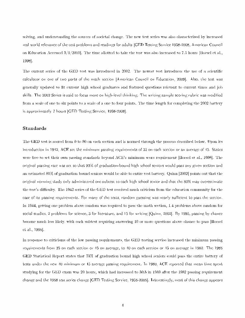
Standards

The GED test is scored from 0 to 80 on each section and is normed through the process described below. Upon its

introduction in 1942, ACE set the minimum passing requirements of 35 on each section or an average of 45. States

were free to set their own passing standards beyond ACE's minimum score requirement [Boesel et al., 1998]. The

original passing rate was set so that 93% of graduation-bound high school seniors would pass any given section and

an estimated 80% of graduation-bound seniors would be able to entire test battery. Quinn [2002] points out that the

original norming study only administered one subtest to each high school senior and that the 80% may overestimate

the test's di�culty. The 1942 series of the GED test received much criticism from the education community for the

ease of its passing requirements. For many of the tests, random guessing was nearly su�cient to pass the section.

In 1944, getting one problem above random was required to pass the math section, 1.4 problems above random for

social studies, 2 problems for science, 3 for literature, and 15 for writing [Quinn, 2002]. By 1995, passing by chance

became much less likely, with each subtest requiring answering 10 or more questions above chance to pass [Boesel

et al., 1998].

In response to criticisms of the low passing requirements, the GED testing service increased the minimum passing

requirements from 35 on each section or 45 on average, to 40 on each section or 45 on average in 1982. The 1988

GED Statistical Report states that 75% of graduation-bound high school seniors could pass the entire battery of

tests under the new 40 minimum or 45 average passing requirement. In 1980, ACE reported that mean time spent

studying for the GED exam was 20 hours, which had increased to 30.5 in 1989 after the 1982 passing requirement

change and the 1988 test series change [GED Testing Service, 1958-2008]. Interestingly, most of this change appears

4

to be in the number of people studying over 100 hours, which increased from 11.8% to 24.2%.

The di�culty of the test was again increased in 1998 when the minimum passing score was raised to 40 on each

section and 45 average. Given the new 40 and 45 test requirement, only 67% of graduation bound high school

seniors were estimated to be able to pass all �ve tests [GED Testing Service, 1958-2008]. The introduction of the

2002 test series again created the test's di�culty. The new test score scale ranged from 200 to 800, representing a

simple di�erence in scaling from the old 20 to 80 range, but now the minimum passing requirements were increased

from 40 and 45 on each section to 410 on each section and a mean score of 450 across all sections. The GED

Statistical Reports quote that only 60% of graduation bound seniors would be able to pass all �ve of the tests [GED

Testing Service, 1958-2008].

Norming and Scoring

The 2002 GED test is scored from 200 to 800 and also awarded a 1 to 99 percentile rank on each of the �ve tests.

The test is normed against graduation-bound high school seniors during re-norming and equating studies conducted

in 1943, 1955, 1967, 1977, 1980, 1987, 1996, 2000, 2002, 2003, and 2005 [Boesel et al. 1998, American Council

on Education 1993, American Council on Education 2009]. For each subtest, scores are constructed so that 500

represents the median and 100 the standard deviation of the graduation bound high school seniors test scores. For

the writing test, the multiple choice score and writing sample score are weighted together. The percentile score

each test taker receives is the percentile of graduation-bound high school seniors achieving this score. Speci�cally,

the 2002 GED Technical Manual says:

�For each test in the battery, cumulative proportion distributions of scores were pre-smoothed using

the log-linear method. These smoothed distributions were independently normalized by converting the

midpoint of each interval (i.e., raw score unit) in the smoothed distribution to a standard normal deviate,

or z-score. These scores were transformed linearly to produce a distribution of standard scores with a

mean of 500 and a standard deviation of 100. Scores more than three standard deviations from the

mean were truncated to conform to the 200 to 800 range.�(pg 40)

Prior to 2002, the test was scored on a scale of 20 to 80 with the same 1 to 99 percentile rank. The test was normed

so that the median score was 50, with standard deviation of 10 for graduation-bound high school seniors. The GED

testing service stresses that adding a zero to old test scores does not make them comparable, as there have been

other changes in material covered and in the high school population over time [American Council on Education,

5

2009]. For that reason, this criticism also applies to comparing GED test scores across any two test series even

when the scale had remained consistent. For further information on the norming and scoring procedures see the

GED Technical Manuals for the 2002 and 1988 series.

The GED Testing Service (GEDTS) has been criticized for the low-stakes or no-stakes testing environment under

which the norming groups take the test. Norming tests involves giving one to three of the �ve tests to graduation-

bound seniors in high school. The graduating seniors do not face incentives to do well on the test and their scores

may understate their true ability. Thus, the ability of GED test takers may be overstated relative to the true

distribution of high school graduates' abilities [Quinn 2002, Sundre 1999].

Another potential criticism of the GED test is that the GEDTS scores the test according to Classical Test Theory

(CTT) rather than according to Item Response Theory (IRT). IRT takes into consideration each problem's e�ec-

tiveness at discriminating ability and the di�culty of the problem. The use of classical test theory rather than IRT

may lead to more noise in the data and less ability to evaluate the actual cognitive ability of those passing the test.

For an overview of IRT and CTT see Fan [1998].

B Descriptions of Key Data Sets

B.1 National Longitudinal Survey of Youth 1979 (NLSY79)

Source: http://www.bls.gov/nls/nlsy79.htm

Description: The NLSY79 includes both a randomly chosen sample of 6,111 U.S. youth and a supplemental sample

of 5,295 randomly chosen Black, Hispanic, and non-Black non-Hispanic economically disadvantaged youths. Both

of these samples are drawn from the civilian population. In addition, there is a small sample of individuals (1,280)

who were enrolled in the military in 1979. All youths were age 14-22 in 1979 and were interviewed annually

beginning in 1979 and then biennially starting in 1994. The NLSY79 data contain a rich variety of measures on

family background, schooling histories, work histories, welfare histories, marital and fertility choices, and geographic

location in each year.

B.1.1 Cognitive Measures

Armed Forces Qualifying Test (AFQT) The NLSY79 contains a battery of 10 tests that measure knowledge

and skill in the following areas: (1) general science; (2) arithmetic reasoning; (3) word knowledge; (4) paragraph

6

comprehension; (5) numerical operations; (6) coding speed; (7) auto and shop information; (8) mathematical

knowledge; (9) mechanical comprehension; and (10) electronics information. These tests were administered to all

sample members in 1980. The tests used in the analyses of Heckman et al. [2006] and Heckman and Urzua [2010]

are: (i) arithmetic reasoning (ASVAB1), (ii) word knowledge (ASVAB2), (iii) paragraph comprehension (ASVAB3),

(iv) mathematical knowledge (ASVAB4), and (v) coding speed (ASVAB5) . A composite score derived from select

sections of the battery can be used to construct an approximate and uno�cial Armed Forces Quali�cations Test

(AFQT) score for each youth.The AFQT is a general measure of trainability and a primary criterion of enlistment

eligibility for the Armed Forces, and it has been used extensively as a measure of cognitive skills in the literature.

B.1.2 Noncognitive Measures

Rotter Internal-External Locus of Control Scale The Rotter Internal-External Locus of Control Scale,

collected as part of the 1979 interviews, is a four-item abbreviated version of a 23-item forced choice questionnaire,

itself adapted from the 60-item Rotter scale developed by Rotter (1966). The scale is designed to measure the extent

to which individuals believe they have control over their lives, i.e., self-motivation and self-determination, (internal

control) as opposed to the extent that the environment (i.e., chance, fate, luck) controls their lives (external control).

The scale is scored in the internal direction: the higher the score, the more internal the individual. Individuals are

�rst shown four sets of statements (displayed in Table B.1.2 below) and asked which of the two statements is closer

to their own opinion. They are then asked whether that statement is much closer or slightly closer to their opinion.

These responses are used to generate four-point scales for each of the paired items, which are then averaged to

create one Rotter Scale score for each individual.

Table 1: Rotter Internal-External Locus of Control Scale

Question 1 (Rotter 1)(a) What happens to me is my own doing.

(b) Sometimes I feel that I don't have enough control over the direction my life is taking.

Question 2 (Rotter 2)When I make plans,

(a) I am almost certain that I can make them work.

(b) It is not always wise to plan too far ahead, because many things turn out to be a matter of good or bad fortune anyhow.

Question 3 (Rotter 3)(a) Getting what I want has little or nothing to do with luck.

(b) Many times we might just as well decide what to do by flipping a coin

Question 4 (Rotter 4)(a) Many times I feel that I have little influence over the things that happen to me.

(b) It is impossible for me to believe that chance or luck plays an important role in my life.

Table S27. Rotter Internal-External Locus of Control Scale

7

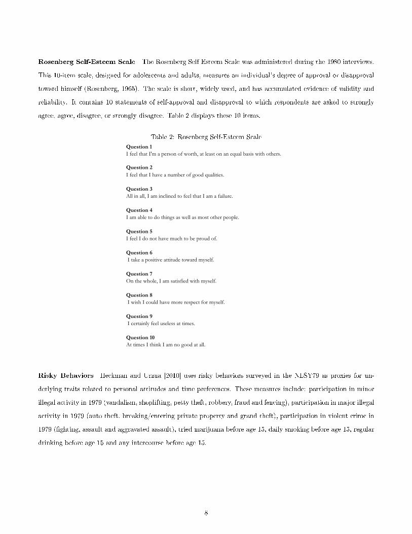
Rosenberg Self-Esteem Scale The Rosenberg Self-Esteem Scale was administered during the 1980 interviews.

This 10-item scale, designed for adolescents and adults, measures an individual's degree of approval or disapproval

toward himself (Rosenberg, 1965). The scale is short, widely used, and has accumulated evidence of validity and

reliability. It contains 10 statements of self-approval and disapproval to which respondents are asked to strongly

agree, agree, disagree, or strongly disagree. Table 2 displays these 10 items.

Table 2: Rosenberg Self-Esteem Scale

Question 1 I feel that I'm a person of worth, at least on an equal basis with others.

Question 2 I feel that I have a number of good qualities.

Question 3All in all, I am inclined to feel that I am a failure.

Question 4I am able to do things as well as most other people.

Question 5I feel I do not have much to be proud of.

Question 6 I take a positive attitude toward myself.

Question 7On the whole, I am satisfied with myself.

Question 8 I wish I could have more respect for myself.

Question 9 I certainly feel useless at times.

Question 10At times I think I am no good at all.

Table S28. Rosenberg Self-Esteem Scale

Risky Behaviors Heckman and Urzua [2010] uses risky behaviors surveyed in the NLSY79 as proxies for un-

derlying traits related to personal attitudes and time preferences. These measures include: participation in minor

illegal activity in 1979 (vandalism, shoplifting, petty theft, robbery, fraud and fencing), participation in major illegal

activity in 1979 (auto theft, breaking/entering private property and grand theft), participation in violent crime in

1979 (�ghting, assault and aggravated assault), tried marijuana before age 15, daily smoking before age 15, regular

drinking before age 15 and any intercourse before age 15.

8

B.2 National Longitudinal Survey of youth 1997 (NLSY97)

Source: http://www.bls.gov/nls/nlsy97.htm

Description: The survey documents the transition from school to work of 8,894 individuals. Two subsamples

comprise the NLSY97 cohort: 6,748 respondents representative of people living in the United States in 1997 who

were born during the years 1980-1984, and 2,236 respondents designed to over-sample black and Hispanic people

living in the US during the same period as the cross-sectional sample. Information was gathered from a youth

questionnaire, parent questionnaire, screener/household informant questionnaire, household income updates, and

school and transcript surveys.

B.2.1 Cognitive Measures

Armed Forces Qualifying Test (AFQT) Source: http://www.bls.gov/nls/handbook/2005/nlshc2.pdf.

Over the summer and fall of 1997 and the winter of 1998, NLSY97 respondents took the computer adaptive version

of the Armed Services Vocational Aptitude Battery (CAT-ASVAB). The CAT-ASVAB comprises 12 separate tests.

The U.S. Department of Defense, which funded the administration of the CAT-ASVAB for NLSY97 respondents,

administered the tests to two additional samples of youths. The �rst group consisted of a nationally representative

sample of students who were expected to be in the 10th through 12th grades in the fall of 1997. This sample included

many of the youths who participated in the NLSY97. The second group was a nationally representative sample of

people who were 18-to-23-year-olds (as of June 1, 1997), the principal age range of potential military recruits. The

Department of Defense used data for this older group to establish national norms for the score distribution of the

ASVAB and the Armed Forces Quali�cation Test (AFQT), which is based on a formula that includes the scores for

the �rst four tests of the ASVAB.

The NLSY97 data �le includes ASVAB scores but does not include an o�cial AFQT score. The Department of

Defense chose not to calculate AFQT scores for the NLSY97 sample because of doubts about whether the national

norms for 18-to-23-year-olds are appropriate for test-takers who are younger. As a substitute for the AFQT score,

NLS sta� members devised a formula for an �ASVAB Math/Verbal score� that is believed to approximate closely

the formula that the Department of Defense used to estimate AFQT scores for the sample of 18-to-23-year-olds.

The formula devised by NLS sta� has been used to create a variable on the NLSY97 data �le that is similar to the

AFQT scores.

9

B.2.2 Construction of NLSY97 Indices of Home Environment

Family Routine Index 1997 Source: www.nlsinfo.org/preview.php?�lename=appendix9.pdf. Pg. 41-45

Family Routine Index is modi�ed from the Family Routines Inventory (FRI) (Jenson, James, Bryce, & Hartnett,

1983).

Questions:

1. In a typical week, how many days from 0 to 7 do you eat dinner with your family?

2. In a typical week, how many days from 0 to 7 does housework get done when it is supposed to, for example

cleaning up after dinner, doing dishes, or taking out the trash?

3. In a typical week, how many days from 0 to 7 do you do something fun as a family such as play a game, go

to a sporting event, go swimming and so forth?

4. In a typical week, how many days from 0 to 7 do you do something religious as a family such as go to church,

pray or read the scriptures together?

These responses were measured on an 8-point scale. The Family Routines Index was created by summing responses

to these four items; scores could range from 0 to 28. Higher scores indicate more days spent in routine activities

with the family. The scores were standardized with mean zero, standard deviation one.

Family/Home Risk Index 1997 Source: www.nlsinfo.org/preview.php?�lename=appendix9.pdf. Pg. 107-114

The Family/Home Risk Index is based on Caldwell and Bradley's Home Observation for Measurement of the

Environment (HOME; Caldwell & Bradley, 1984) and on personal correspondence with Robert Bradley on the

development of a HOME index for adolescents.

Questions:

Home Physical Environment

1. In the past month, has your home usually had electricity and heat when you needed it?

2. How well kept is the interior of the home in which the youth respondent lives?

3. How well kept is the exterior of the housing unit where the youth respondent lives?

10

Neighborhood

1. How well kept are most of the buildings on the street where the adult/youth resident lives?

2. When you went to the respondent's neighborhood/home, did you feel concerned for your safety?

3. In a typical week, how many days from 0 to 7 do you hear gunshots in your neighborhood?

Enriching Activities

1. In the past month, has your home usually had a quiet place to study?

2. In the past month, has your home usually had a computer?

3. In the past month, has your home usually had a dictionary?

Religious Behavior

1. In the past 12 months, how often have you attended a worship service (like church or synagogue service or

mass)?

2. In a typical week, how many days from 0 to 7 do you do something religious as a family such as go to church,

pray or read the scriptures together?

School Involvement

1. In the last three years have you or your [spouse/partner] attended meetings of the parent-teacher organization

at [this youth]'s school?

2. In the last three years have you or your [spouse/partner] volunteered to help at the school or in the classroom?

Family Routines

1. In a typical week, how many days from 0 to 7 do you eat dinner with your family?

2. In a typical week, how many days from 0 to 7 does housework get one when it is supposed to, for example

cleaning up after dinner, doing dishes, or taking out the trash?

3. In a typical week, how many days from 0 to 7 do you do something fun as a family such as play a game, go

to a sporting event, go swimming and so forth?

11

4. In a typical [school week/work week/week], did you spend any time watching TV?

5. In that week, on how many weekdays did you spend time watching TV?

6. On those weekdays, about how much time did you spend per day watching TV?

Parent Characteristics

1. Physical disabilities: Hard of hearing? Unable to see well? Physical handicapped?

2. Mental disabilities: Mentally handicapped? Command of English is poor? Unable to read?

3. Alcohol/Drug disability: Under the in�uence of alcohol or drugs?

Parenting

1. Monitoring Scale (youth report) for youth's residential mother

2. Monitoring Scale (youth report) for youth's residential father: If neither parent high on monitoring (Score

less than 6) = Risk; If either parent high on monitoring (Score greater than 6) = Not coded as Risk

3. Parent-Youth Relationship Scale (youth report) for residential mother

4. Parent-Youth Relationship Scale (youth report) for residential father: If neither parent was warm (Score less

than 18) = Risk; If either parent was warm (Score greater than 18) = Not coded as Risk

5. When you think about how she (residential mother) acts toward you, in general, would you say she is very

supportive, somewhat supportive, or not very supportive?

6. In general, would you say that she (residential mother) is permissive or strict about making sure you did what

you were supposed to do?

7. When you think about how he (residential father) acts toward you, in general, would you say he is very

supportive, somewhat supportive, or not very supportive?

8. In general, would you say that he (residential father) is permissive or strict about making sure you did what

you were supposed to do?

Index is created in a way that each item (or set of items) was coded into risk categories, so that 1 = Risk and 0 =

Not coded as Risk. The items were then summed to produce a composite score for the Family/Home Risk Index;

ranging from 0 to 21. Higher scores indicate a higher risk environment.The scores were standardized with mean zero,

standard deviation one.

12

Physical Envioronment Index 1997 Source: www.nlsinfo.org/preview.php?�lename=appendix9.pdf. Pg. 115-

120

This index was developed by researchers at Child Trends. The items are a sub-set of items from the Family/Home

Risk Index, however for this index not all variables were coded as dichotomous indicators of risk.

B.3 Current Population Survey - March Supplement (CPS March)

Source: http://www.unicon.com and http://nces.ed.gov/surveys/cps/

Description: The Current Population Survey (CPS) is a monthly survey of approximately 50,000 households that

are selected scienti�cally in the 50 states and the District of Columbia. The CPS has been conducted for more

than 50 years by the Census Bureau for the Bureau of Labor Statistics. The CPS collects data on the social and

economic characteristics of the civilian, non-institutional population, including information on income, education,

and participation in the labor force. Each month, a "basic" CPS questionnaire is used to collect data on par-

ticipation in the labor force about each member 15 years old and over in every sample household. In addition,

supplemental questionnaires are administered to collect information on other topics. In each household, the Bureau

seeks information from a knowledgeable adult household member (known as the "household respondent"). That

respondent answers all the questions on all of the questionnaires for all members of the household.

The Annual Demographic Survey or March CPS supplement is the primary source of detailed information on income

and work experience in the United States. The March CPS is used to generate the annual Population Pro�le of

the United States, reports on geographical mobility and educational attainment, and detailed analyses of money

income and poverty status.

B.4 Current Population Survey - October Supplement (CPS October)

Source: http://www.unicon.com and http://nces.ed.gov/surveys/cps/

Description: Since 1968, NCES has funded the CPS October Supplement. The October Supplement gathers more

detailed data on schooling enrollment and educational attainment among school aged youth. Unlike the CPS

March and Census Surveys, in 1988 the CPS October supplement began to distinguish between GED recipients and

regular high school graduates. These variables are available for 16-24 year olds from 1988-1992 and 16-29 year olds

thereafter.

13

B.5 High School and Beyond Sophomore Cohort (HSB)

Source: http://nces.ed.gov/surveys/hsb/

Description: The High School and Beyond Sophomore Cohort (HSB) data set provides a valuable source of panel

information on 27,204 sophomores. The base year survey was conducted in spring 1980. Three follow-up surveys

were conducted in 1982, 1984, and 1992. The study design provided for a strati�ed national probability sample

of over 1100 secondary schools as the �rst stage selection. In the second stage, 36 sophomores were selected in

each school. Public schools with high percentages of Hispanic students, Catholic schools with high percentages

of minority group students, alternative public schools and private schools with high-achieving students were over

sampled. Individuals were asked about their family background, ethnicity, schooling histories, and labor force

histories.

The HSB data are valuable as another data source for cohorts born around the time of the NLSY79 survey which

provides detailed schooling histories and educational attainment measures. A weakness of the HSB data is that

the survey sample starts with students who are enrolled in the 10th grade in 1980. This sample design will tend to

overstate high school graduation rates since those who dropped out prior to reaching 10th grade will be excluded.

14

C Supplementary Descriptive Tables

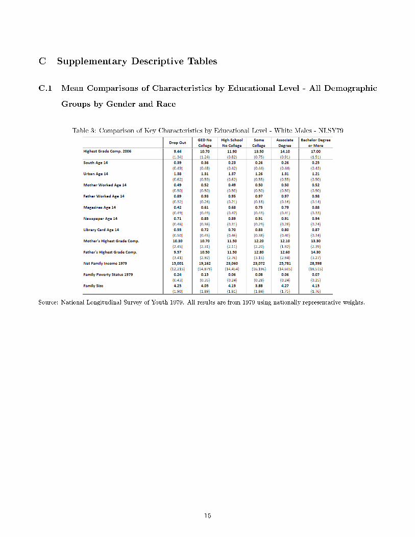
C.1 Mean Comparisons of Characteristics by Educational Level - All Demographic

Groups by Gender and Race

Table 3: Comparison of Key Characteristics by Educational Level - White Males - NLSY79

Source: National Longitudinal Survey of Youth 1979. All results are from 1979 using nationally representative weights.

15

Table 4: Comparison of Key Characteristics by Educational Level - White Females - NLSY79


Table 5: Comparison of Key Characteristics by Educational Level - Black Males - NLSY79


16

Table 6: Comparison of Key Characteristics by Educational Level - Black Females - NLSY79


Table 7: Comparison of Key Characteristics by Educational Level - Hispanic Males - NLSY79


17

Table 8: Comparison of Key Characteristics by Educational Level - Hispanic Females - NLSY79


Table 9: Comparison of Key Characteristics by Educational Level - White Males - NLSY97


18

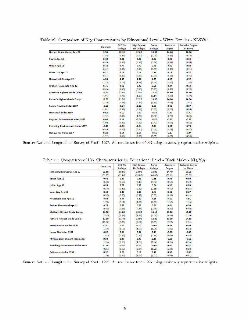
Table 10: Comparison of Key Characteristics by Educational Level - White Females - NLSY97


Table 11: Comparison of Key Characteristics by Educational Level - Black Males - NLSY97


19

Table 12: Comparison of Key Characteristics by Educational Level - Black Females - NLSY97


Table 13: Comparison of Key Characteristics by Educational Level - Hispanic Males - NLSY97


20

Table 14: Comparison of Key Characteristics by Educational Level - Hispanic Females - NLSY97


21

C.2 Males vs. Females: Reported Reasons for Dropping Out

Table 15: Primary Reasons High School Dropouts Left School

Source: Reproduced from Rumberger [1983].

22

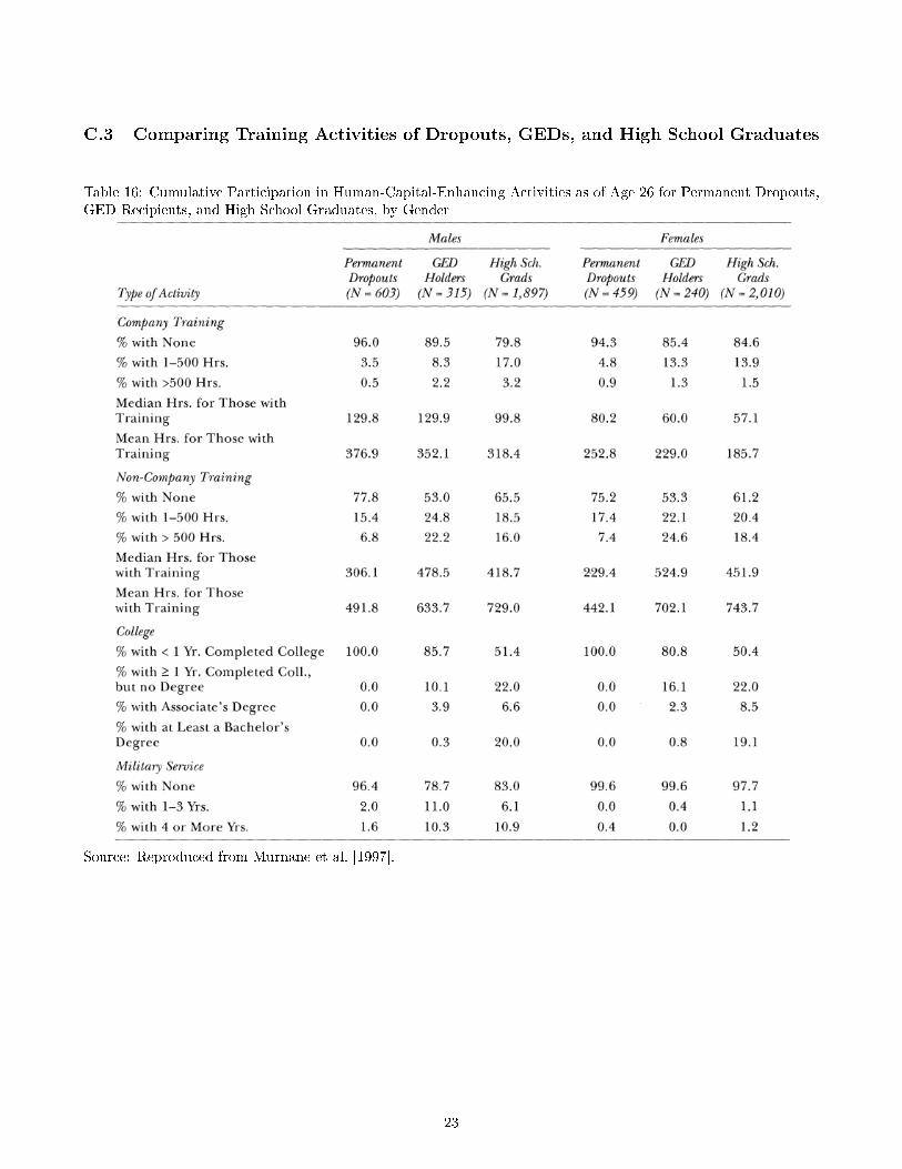
C.3 Comparing Training Activities of Dropouts, GEDs, and High School Graduates

Table 16: Cumulative Participation in Human-Capital-Enhancing Activities as of Age 26 for Permanent Dropouts,GED Recipients, and High School Graduates, by Gender

Source: Reproduced from Murnane et al. [1997].

23

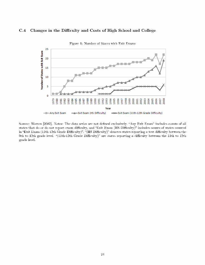
C.4 Changes in the Di�culty and Costs of High School and College

Figure 1: Number of States with Exit Exams

Source: Warren [2007]. Notes: The data series are not de�ned exclusively. �Any Exit Exam� includes counts of allstates that do or do not report exam di�culty, and �Exit Exam (HS Di�culty)� includes counts of states countedin �Exit Exam (11th-12th Grade Di�culty)�. �(HS Di�culty)� denotes states reporting a test di�culty between the9th to 12th grade level. �(11th-12th Grade Di�culty)� are states reporting a di�culty between the 11th to 12thgrade level.

24

Figure 2: Trends in Carnegie Units Required for High School Graduation

Source: National Center for Educational Statistics. Notes: Carnegie Units are a standardized class hours measure-ment roughly equivalent to taking once class for one academic year. The increase in the 1980s corresponds to thepublication of the National Commission on Excellence in Education's report �Nation at Risk� in 1983. The reportspeci�cally called for increased graduation requirements, prescribing minimum years of instruction in each of severalcore subjects.

Figure 3: Tuition Costs of Community College, and Public and Private 4-Year College

Source: Digest of Educational Statistics (various years). Note: All numbers reported in 2008 dollars.

25

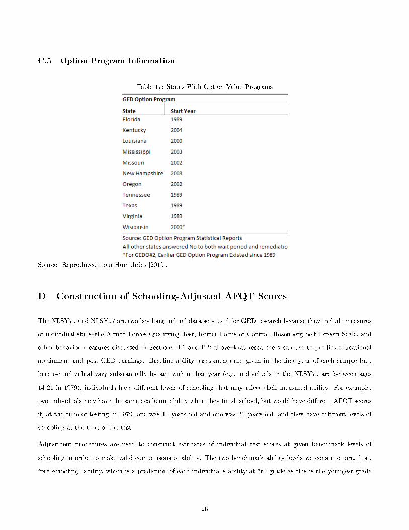
C.5 Option Program Information

Table 17: States With Option Value Programs

Source: Reproduced from Humphries [2010].

D Construction of Schooling-Adjusted AFQT Scores

The NLSY79 and NLSY97 are two key longitudinal data sets used for GED research because they include measures

of individual skills�the Armed Forces Qualifying Test, Rotter Locus of Control, Rosenberg Self-Esteem Scale, and

other behavior measures discussed in Sections B.1 and B.2 above�that researchers can use to predict educational

attainment and post-GED earnings. Baseline ability assessments are given in the �rst year of each sample but,

because individual vary substantially by age within that year (e.g. individuals in the NLSY79 are between ages

14-21 in 1979), individuals have di�erent levels of schooling that may a�ect their measured ability. For example,

two individuals may have the same academic ability when they �nish school, but would have di�erent AFQT scores

if, at the time of testing in 1979, one was 14 years old and one was 21 years old, and they have di�erent levels of

schooling at the time of the test.

Adjustment procedures are used to construct estimates of individual test scores at given benchmark levels of

schooling in order to make valid comparisons of ability. The two benchmark ability levels we construct are, �rst,

�pre-schooling� ability, which is a prediction of each individual's ability at 7th grade as this is the youngest grade

26

that (nearly) all of the NLSY79 sample had reached when they were tested. This ability is relative to a level of

schooling that is common to all individuals. The second, termed �post-schooling� ability, is a prediction of each

individual's ability at the level of schooling that they will eventually complete. This measure is used to compare

the ability that individuals have when they �rst enter the job market.

The GED literature features a range of approaches used to construct comparable abilities, but most commonly

makes either simple adjustments or no adjustments at all. We identify four approaches and contrast the bias in

estimating true schooling-adjusted test scores associated with each method:

1. �No Adjustment� - No adjustment is made to account for the e�ect of schooling on AFQT scores, which

are used to adjust for ability in outcomes equations,1 as in Murnane et al. [1999];

2. �Simple Adjustment (SA)� - Researchers regress AFQT scores on measures of completed schooling, and

use the residual as an estimate of the individual's raw ability �before� schooling as in Kenkel et al. [2006];

3. �Heterogenous Adjustment (HA)� - This is our approach, which improves on the Simple Adjustment

procedure by allowing the mean returns to additional years of schooling to vary by an individual's �nal

educational attainment;

4. �Factor Augmentation Adjustment� - This approach improves on the Heterogeneous Adjustment by

allowing returns to schooling to vary by levels of each individual's latent ability type. Hansen et al. [2004]

(HHM), produce an adjusted distribution of abilities, rather than only adjusting the mean.

Implementation of Ability Adjustments

An individual's ability at a benchmark level of schooling is estimated as her observed score minus her estimated

academic growth between the benchmark and time of the test. Individual ability is only sampled once in the

NLSY79 and NLSY97, so this academic growth cannot be estimated by looking within individual growth trajectories.

Adjustment approaches di�er by how they infer academic growth across levels of schooling.

Simple Adjustment Procedure (Common in the GED Literature) The Simple Adjustment procedure is

the most commonly used in the literature. It estimates growth related to schooling as the di�erence between average

achievement levels associated with di�erent levels of schooling.

1Papers using unadjusted methods commonly restrict their sample to speci�c age ranges and educational attainments to minimizebias, e.g. Cameron and Heckman [1993].

27

Let St and SF denote random variables describing respectively the level of schooling characterizing individuals at

the time that they are tested (st) and their level of �nal schooling (sF ). Let st and sF denote realized values of

these random variables.2 Let s∗ denote a benchmark level of schooling, where s0 and sF respectively denote the

baseline and �nal levels of schooling. Consider an individual with test score T (St = st, SF = sF ). Under the Simple

Adjustment procedure, individual ability at counterfactual level of schooling s∗ is estimated as

T̂SA(St = s

∗, SF = sF ) = T (St = st, SF = sF ) − [E (T ∣St = st) −E (T ∣St = s∗)] (1)

.

Heterogeneous Adjustment Procedure (Our Method) The Heterogeneous Adjustment procedure used in

the paper recognizes that the expected returns an individual receives from a given level of schooling may be

associated with the �nal level of schooling that they complete. For example, it may be that individuals who go on

to complete college receive a di�erent level of educational bene�t from 9th grade than would eventual dropouts.

Hansen, Heckman, and Mullen [2004] document such di�erences. In contrast with the Simple Adjustment procedure,

this method calculates estimates of growth separately for each subsample of individuals with di�erent levels of �nal

schooling.

Formally, this adjustment is

T̂HA(St = s0, SF = sF ) = T (St = st, SF = sF ) − [E (T ∣ St = st,SF = sF)−E (T ∣ St = s∗,SF = sF)] (2)

.

Comparisons of Bias Across Adjustment Models

In this section we explore the sources of bias for each method using the HHM framework as the baseline model. It

is

T (st) = µ (st) + λ (st) f + ε (st) (3)

where µ (st) is an intercept term for test scores at schooling level st, λ (st) is a factor loading that depends on st,

f is the individual latent ability factor, ε (st) is measurement error. The functional dependence of µ, λ and ε on st

2In our approach, the index of �nal level of schooling completed not perfectly ordered, as by a measure of total years of schooling.Our classi�cation di�erentiates obtained levels of schooling by the route that was taken. For example, a two-year college graduate who�nished high school is distinguished from one who completed a GED.

28

allows average ability, rates of transformation of latent ability into tested ability, and distributions of heterogeneous

ability to vary by each given schooling level. Identi�cation of this model is discussed and implemented in Hansen

et al. [2004].

We assume that st is mean independent of f given SF :

E [f ∣St = st, SF = sF ] = E [f ∣SF = sF ] (4)

.

Bias Associated with Simple Adjustment (SA) Procedure Using the expression for individual test scores

given in equation (3), the SA adjustment method in equation (1) is

T̂SA(St = s

∗, sF ) = T (st, sF ) − [µ (st) + λ (st)E (f ∣St = st)]

´¹¹¹¹¹¹¹¹¹¹¹¹¹¹¹¹¹¹¹¹¹¹¹¹¹¹¹¹¹¹¹¹¹¹¹¹¹¹¹¹¹¹¹¹¹¹¹¹¹¹¹¹¹¹¹¹¹¹¹¹¹¹¹¹¹¹¹¹¹¹¹¹¹¹¹¹¹¹¹¹¹¹¹¹¹¹¹¹¹¹¹¹¹¸¹¹¹¹¹¹¹¹¹¹¹¹¹¹¹¹¹¹¹¹¹¹¹¹¹¹¹¹¹¹¹¹¹¹¹¹¹¹¹¹¹¹¹¹¹¹¹¹¹¹¹¹¹¹¹¹¹¹¹¹¹¹¹¹¹¹¹¹¹¹¹¹¹¹¹¹¹¹¹¹¹¹¹¹¹¹¹¹¹¹¹¹¹¶

contructed using results from a regression of T (st,sF )on st

+ [µ (s∗) + λ (s∗)E (f ∣St = s∗)]

´¹¹¹¹¹¹¹¹¹¹¹¹¹¹¹¹¹¹¹¹¹¹¹¹¹¹¹¹¹¹¹¹¹¹¹¹¹¹¹¹¹¹¹¹¹¹¹¹¹¹¹¹¹¹¹¹¹¹¹¹¹¹¹¹¹¹¹¹¹¹¹¹¹¹¹¹¹¹¹¹¹¹¹¹¹¹¹¹¹¹¹¹¹¹¹¹¹¸¹¹¹¹¹¹¹¹¹¹¹¹¹¹¹¹¹¹¹¹¹¹¹¹¹¹¹¹¹¹¹¹¹¹¹¹¹¹¹¹¹¹¹¹¹¹¹¹¹¹¹¹¹¹¹¹¹¹¹¹¹¹¹¹¹¹¹¹¹¹¹¹¹¹¹¹¹¹¹¹¹¹¹¹¹¹¹¹¹¹¹¹¹¹¹¹¶

contructed using results from a regression of T (s∗, sF )on s∗

The bias associated with this adjustment is

SA Bias = T̂SA(St = s

∗, sF ) − T (St = s∗, sF )

= T (st, sF ) − [µ (st) + λ (st)E (f ∣St = st)] + [µ (s∗) + λ (s∗)E (f ∣St = s∗)] − T (St = s

∗, sF )

+ [µ (s∗) + λ (s∗)E (f ∣St = s∗)] − T (St = s

∗, sF )

= [µ (st) + λ (st) f + ε (st)] − [µ (st) + λ (st)E (f ∣St = st)]

+ [µ (s∗) + λ (s∗)E (f ∣St = s∗)] − [µ (s∗) + λ (s∗) f + ε (s∗)]

= ε (st) − ε (s∗) + λ (st) [f −E (f ∣St = st)] − λ (s∗) [f −E (f ∣St = s

∗)]

.In general λ(st) ≠ λ(s∗) and E (f ∣ St = st) ≠ E (f ∣ St = st) so there is bias in the means.

29

Bias Associated with the Heterogeneous Adjustment (HA) Procedure Using the expression for individ-

ual test scores given in equation (3), the HA adjustment method in equation (2) is

T̂HA(St = s

∗, sF ) = T (st, sF ) − [µ (st) + λ (st)E (f ∣St = st, SF = sF )]

´¹¹¹¹¹¹¹¹¹¹¹¹¹¹¹¹¹¹¹¹¹¹¹¹¹¹¹¹¹¹¹¹¹¹¹¹¹¹¹¹¹¹¹¹¹¹¹¹¹¹¹¹¹¹¹¹¹¹¹¹¹¹¹¹¹¹¹¹¹¹¹¹¹¹¹¹¹¹¹¹¹¹¹¹¹¹¹¹¹¹¹¹¹¹¹¹¹¹¹¹¹¹¹¹¹¹¹¹¹¹¹¹¹¹¹¹¹¹¹¹¹¹¹¹¹¹¹¹¸¹¹¹¹¹¹¹¹¹¹¹¹¹¹¹¹¹¹¹¹¹¹¹¹¹¹¹¹¹¹¹¹¹¹¹¹¹¹¹¹¹¹¹¹¹¹¹¹¹¹¹¹¹¹¹¹¹¹¹¹¹¹¹¹¹¹¹¹¹¹¹¹¹¹¹¹¹¹¹¹¹¹¹¹¹¹¹¹¹¹¹¹¹¹¹¹¹¹¹¹¹¹¹¹¹¹¹¹¹¹¹¹¹¹¹¹¹¹¹¹¹¹¹¹¹¹¹¹¶

contructed using results from a regression of T (st,sF )on stcontrolling for SF = sF

+ [µ (s∗) + λ (s∗)E (f ∣St = s∗, SF = sF )]

´¹¹¹¹¹¹¹¹¹¹¹¹¹¹¹¹¹¹¹¹¹¹¹¹¹¹¹¹¹¹¹¹¹¹¹¹¹¹¹¹¹¹¹¹¹¹¹¹¹¹¹¹¹¹¹¹¹¹¹¹¹¹¹¹¹¹¹¹¹¹¹¹¹¹¹¹¹¹¹¹¹¹¹¹¹¹¹¹¹¹¹¹¹¹¹¹¹¹¹¹¹¹¹¹¹¹¹¹¹¹¹¹¹¹¹¹¹¹¹¹¹¹¹¹¹¹¹¹¹¹¹¹¸¹¹¹¹¹¹¹¹¹¹¹¹¹¹¹¹¹¹¹¹¹¹¹¹¹¹¹¹¹¹¹¹¹¹¹¹¹¹¹¹¹¹¹¹¹¹¹¹¹¹¹¹¹¹¹¹¹¹¹¹¹¹¹¹¹¹¹¹¹¹¹¹¹¹¹¹¹¹¹¹¹¹¹¹¹¹¹¹¹¹¹¹¹¹¹¹¹¹¹¹¹¹¹¹¹¹¹¹¹¹¹¹¹¹¹¹¹¹¹¹¹¹¹¹¹¹¹¹¹¹¹¶

contructed using results from a regression of T (s∗, sF )on s∗controlling for SF = sF

The bias associated with our approach is given by

HA Bias = T̂HA(St = s0, sF ) − T (St = s0, sF )

= T (st, sF ) − [µ (st) + λ (st)E (f ∣St = st, SF = sF )]

+ [µ (s0) + λ (s0)E (f ∣St = s∗, SF = sF )] − T (St = s0, sF )

= [µ (st) + λ (st) f + ε (st)] − [µ (st) + λ (st)E (f ∣SF = sF )]

+ [µ (s0) + λ (s0)E (f ∣SF = sF )] − [µ (s0) + λ (s0) f + ε (s0)]

= ε (st) − ε (s0) + [λ (st) − λ (s0)] [f −E (f ∣SF = sF )]

where the third equality uses the mean independence assumption re�ected in equation (4). This method avoids

bias in the means.

30

E Supplementary Tables

E.1 Detailed Literature Summary Tables

Table 18: Detailed Literature Summary of Research on Labor Market and Educational Attainment Bene�tsData Set Time Period Population Outcomes GED Effect1 Effect Estimate Other Conditioning Variables Identification

Strategy

NLSY79 1979-1987 W M, A=28 Wg 1/0 .037 Unemp, R, Year of BirthWg 1/0 .101 Exp, Ten, Ten2, Unemp, R, Year of BirthHr 1/0 -.074 Unemp, R, Year of BirthWg 1/0 .065 Exp, Ten, Ten2, Unemp, R, Year of Birth, AbHr 1/0 -.19 Unemp, R, Year of Birth, AbWg 1/0 Pre Exp -.045 Unemp, R, Year of BirthWg 1/0 Post Exp .038 Unemp, R, Year of BirthWg 1/0 .015 R, Year of Birth, YoS OLS

NLSY79 1979-1991 M, All R Wg 1/0 .009 R, YoS, Mom's YoS, Exp, Exp2, (Exp, Exp2)*R, (Exp, Exp2)*YoSWg, Exp Post-GED Exp .024**

Hr 1/0 -.059Hr, Exp Post-GED Exp .033

WA FIS F Wg 1/0 -.20 R, Mr, Rg, Year of BirthWA FIS Wg 1/0 -0.22 R, Mr, Rg, Year of Birth, YoSWA FIS Hr 1/0 -4.58* R, Mr, Rg, Year of Birth, AHH, CHH, CBTYWA FIS Hr 1/0 -39.28 R, Mr, Rg, Year of Birth, YoS, CHH, CBTY

Cameron and Heckman (1993)

Murnane, Willett and Boudett (1995)

Cao, Stromsdorfer and Weeks (1996)

Bivariate selection-correction model

1979-1991 1987-1992

1/0 if has or will ever get GED

Bivariate selection-correction model

NLSY79 1979-1991 M and F Pr(OnJT), M, 1/0 1/0 .327 R, YoS, Mom's YoS, Exp, Exp2

Pr(OnJT), F, 1/0 1/0 .328*Pr(OffJT), M, 1/0 1/0 .145 Pr(OffJT), M, Exp Post- Exp .162***Pr(OffJT), F, 1/0 1/0 .691*** Pr(OffJT), F, Exp Post- Exp .077Pr(OffJT), M, 1/0 1/0 2.315*** Pr(OffJT), M, Exp Post- Exp .148**Pr(OffJT), F, 1/0 1/0 2.659*** Pr(OffJT), F, Exp Post- Exp .242***Pr(OffJT), M, 1/0 1/0 .676***Pr(OffJT), M, Exp Post- Exp -.253***

NLSY79 M Wg Post-Exp*LowAb .025* (Exp,Exp2)*(R,LowAb), Unemp, R, YoS, Mom's YoS, PSE, OnJT, OffJTWg .023* (Exp,Exp2)*(R,LowAb), Unemp, R, YoS, Mom's YoSEa 72.6 (Exp,Exp2)*(R,LowAb), Unemp, R, YoS, Mom's YoS, PSE, OnJT, OffJTEa 140.6 (Exp,Exp2)*(R,LowAb), Unemp, R, YoS, Mom's YoS

1979-1991

Individual-level fixed effects



1/0 if has or will ever get GED

M, F, A=16-20, GED Testers Ea (no log) White 1/0 1531** state dum, GED score group dum. G, low-pass-group dum.

M, F, A=16-20, GED Testers Ea (no log) Minority 231

HSB 1980-1991 M Ea .326*** R, YoS, Quartile in Ab, HS*Quartile in Ab OLS.242*** R, YoS, Quartile in Ab, HS*Quartile in Ab, Exp, Exp2

.234*** R, YoS, Quartile in Ab, HS*Quartile in Ab, Exp, Exp2, PSE

HSB 1980-1991 F Ea .223* 1/0 of Top Half of Ab OLS.055 1/0 of Top Half of Ab, Has Children/Is Married, PSE, Exp, Exp 2

Pr(Hrs>0) .85** R, Rg, Mom's Ed, Highest Gr. Compl, Has Children/Is Married LogitYrs Exp 1.295*** OLS

CPS 1998-2001 Wg, M 1/0*FrB*USSch .167*** OLS1/0*FrB*FS .247***

Wg, F 1/0*FrB*USSch .1191/0*FrB*FrS .229***

Murnane, Willett and Tyler (2000)

Tyler, Murnane and Willett (2003)

Clark and Jaeger (2006)

Tyler, Murnane and Willett (2000)

GEDTS Records, and Stud. Ed. Data

Tested in 1990, Ea in

1995

Diff-in-Diff estimates of people with same score and different credential outcome

1/0*(Lowest Quartile of Ab)

M and F, A=20-64, Native and

FrBExp, Exp2 Mr, Birth Region, Residence Region, 4th Order Poly. in ,Calendar Time, Seasonal Dummies

1/0*(Lowest Quartile of Ab)

31

NLSY 1979-2001 M, F Wg, M 1/0 .65*** CCS, Mr w/ spouse present, Yr of Svy, Rg, A, R, A 2, R2 OLSWg, M 1/0 -.008 CCS, Mr w/ spouse present, Yr of Svy, Rg, A, R, A 2, R2, Ab Select'n correctionWg, F 1/0 .113*** CCS, Mr w/ spouse present, Yr of Svy, Rg, A, R, A 2, R2 OLSWg, F 1/0 .017 CCS, Mr w/ spouse present, Yr of Svy, Rg, A, R, A 2, R2, Ab Select'n correction

NLSY 1998-2003 Wg, M 1/0 -.036 CCS, Mr w/ spouse present, Rg, A, A2 Fixed EffectsWg, F 1/0 -.050

CPS no ImpW Wg, M 1/0 .033 CCS, Mr w/ spouse present, Rg, A, A2 Fixed EffectsWg, F 1/0 -.074

CPS FrB Wg, M 1/0 .215 CCS, Mr w/ spouse present, Yr of Svy, Rg, A, R, A 2, R2 OLSWg, F 1/0 .192***

NALS Wg, M 1/0 .066 CCS, Mr w/ spouse present, Yr of Svy, Rg, A, R, A 2, R2 OLS1/0 -.022 CCS, Mr w/ spouse present, Yr of Svy, Rg, A, R, A 2, R2, Ab

Wg, F 1/0 .094** CCS, Mr w/ spouse present, Yr of Svy, Rg, A, R, A 2, R2

1/0 .023 CCS, Mr w/ spouse present, Yr of Svy, Rg, A, R, A 2, R2, AbNALS FrB Wg, M 1/0 .069 CCS, Mr w/ spouse present, Yr of Svy, Rg, A, R, A 2, R2, Ab OLS

Wg, F 1/0 -.010

Heckman and LaFontaine (2006)

E.2 Adverse E�ects of the GED

Figure 4: Di�erence-in-Di�erences Estimates from Increase in GED Di�culty

Source: Reproduced from Heckman et al. [2008].

32

Figure 5: Di�erence-in-Di�erences Estimates from Introduction of GED in California

Source: Reproduced from Heckman et al. [2008].

Figure 6: The E�ect of the GED Option on High School Diplomas and Completers

Source: Reproduced from Humphries [2010].

33

E.3 Dynamic Discrete Choice Model Results

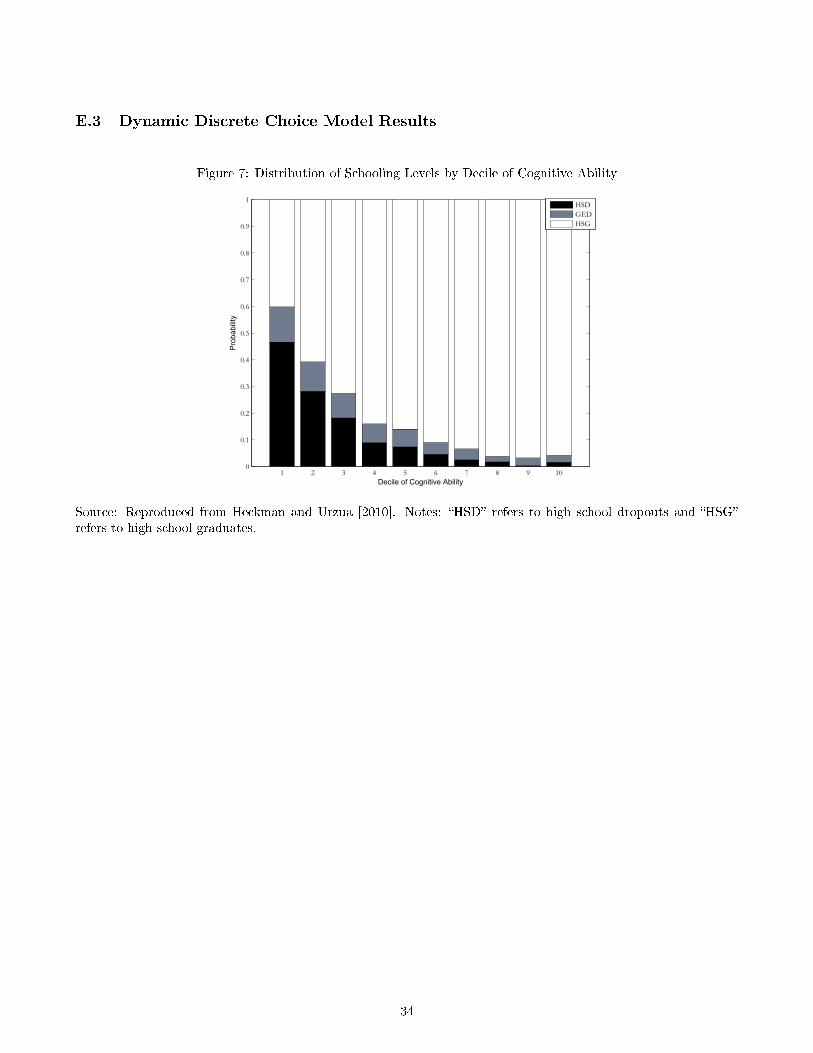
Figure 7: Distribution of Schooling Levels by Decile of Cognitive Ability

1 2 3 4 5 6 7 8 9 100

0.1

0.2

0.3

0.4

0.5

0.6

0.7

0.8

0.9

1

Decile of Cognitive Ability

Pro

babi

lity

Distribution of Schooling Levels by Decile of Cognitive Ability

HSDGEDHSG

Source: Reproduced from Heckman and Urzua [2010]. Notes: �HSD� refers to high school dropouts and �HSG�refers to high school graduates.

34

Figure 8: Distribution of Schooling Levels by Decile of Noncognitive Ability

1 2 3 4 5 6 7 8 9 100

0.1

0.2

0.3

0.4

0.5

0.6

0.7

0.8

0.9

1

Decile of Noncognitive

Pro

babi

lity

Distribution of Schoolig Levels by Decile of Noncognitive Ability

HSDGEDHSG

Source: Reproduced from Heckman and Urzua [2010]. Notes: �HSD� refers to high school dropouts and �HSG�refers to high school graduates.

35

Figure 9: Probability of Dropping Out of High School by Deciles of Cognitive and Noncognitive Abilities

Source: Reproduced from Heckman and Urzua [2010].

36

Figure 10: Probability of GED Certifying by Deciles of Cognitive and Noncognitive Abilities


37

Figure 11: Probability of Finishing High School by Deciles of Cognitive and Noncognitive Abilities


38

Figure 12: Distribution of Option Values for Early GED Certi�cation


39

Figure 13: Distribution of Option Values for College Enrollment (for individuals with HS degree)


40

Figure 14: Distribution of Option Values Associated with Late GED Certi�cation

Source: Reproduced from Heckman and Urzua [2010]. Notes: The model counts individuals as �Late� GED certi�ersif they are uncredentialed dropouts at age 20 and receive a GED afterward.

41

Figure 15: Option Value Associated with (Early) GED Receipt


42

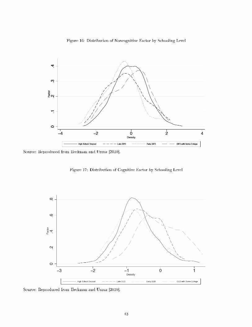
Figure 16: Distribution of Noncognitive Factor by Schooling Level


Figure 17: Distribution of Cognitive Factor by Schooling Level


43

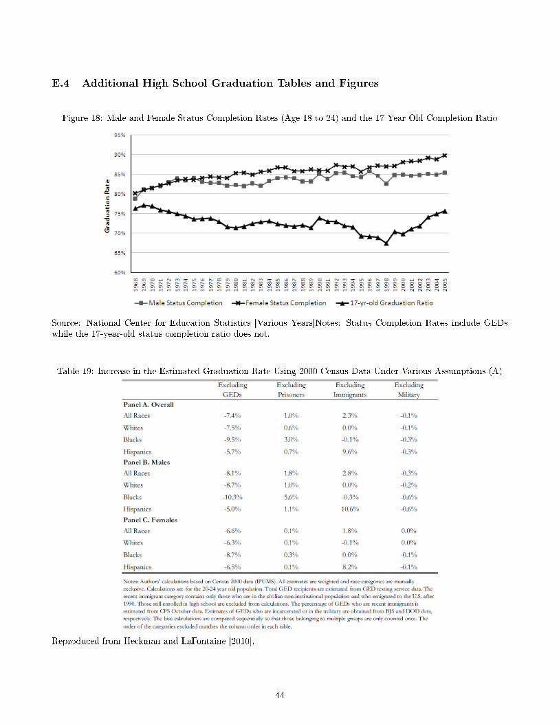
E.4 Additional High School Graduation Tables and Figures

Figure 18: Male and Female Status Completion Rates (Age 18 to 24) and the 17 Year Old Completion Ratio

Source: National Center for Education Statistics [Various Years]Notes: Status Completion Rates include GEDswhile the 17-year-old status completion ratio does not.

Table 19: Increase in the Estimated Graduation Rate Using 2000 Census Data Under Various Assumptions (A)

Reproduced from Heckman and LaFontaine [2010].

44

Table 20: Increase in the Estimated Graduation Rate Using 2000 Census Data Under Various Assumptions (B)

Reproduced from Heckman and LaFontaine [2010]

References

American Council on Education. The Tests of General Educational Development Technical Manual. American

Council on Education, Washington, D.C., 1993.

American Council on Education. Technical Manual: 2002 Series GED Tests. GED Testing Service, Washington,

DC, March 2009.

American Council on Education. History of the GED Tests. http://www.acenet.edu/Content/NavigationMenu/ged/about

/history.htm, Accessed 3/1/2010.

David Boesel, Nabeel Alsalam, and Thomas M. Smith. Educational and Labor Market Performance of GED

Recipients. U.S. Dept. of Education, O�ce of Educational Research and Improvement, National Library of

Education, Washington D.C., 1998.

Stephen V. Cameron and James J. Heckman. The Nonequivalence of High School Equivalents. Journal of Labor

Economics, 11(1, Part 1):1�47, January 1993.

45

X. Fan. Item Response Theory and Classical Test Theory: An Empirical Comparison of their Item/Person Statistics.

Educational and Psychological Measurement, 58:357�381, 1998.

GED Testing Service. Who Took the GED?: GED Statistical Report. American Council on Higher Education,

Washington, DC, 1958-2008.

Karsten T. Hansen, James J. Heckman, and Kathleen J. Mullen. The E�ect of Schooling and Ability on Achievement

Test Scores. Journal of Econometrics, 121(1-2):39�98, July�August 2004.

James J. Heckman and Paul A. LaFontaine. The American High School Graduation Rate: Trends and Levels.

Review of Economics and Statistics, 2010. In press,.

James J. Heckman and Sergio Urzua. The Option Value and Rate of Return to Educational Choices. Unpublished

Manuscript, Northwestern University, 2010.

James J. Heckman, Jora Stixrud, and Sergio Urzua. The E�ects of Cognitive and Noncognitive Abilities on Labor

Market Outcomes and Social Behavior. Journal of Labor Economics, 24(3):411�482, July 2006.

James J. Heckman, Paul A. LaFontaine, and Pedro L. Rodríguez. Taking the Easy Way Out: How the GED

Testing Program Induces Students to Drop Out. Unpublished manuscript, University of Chicago, Department of

Economics, 2008.

Walter E. Hess. How Veterans and Nonveterans May Obtain High School Certi�cation. National Association of

Secondary-School Principals, 1948.

John Eric Humphries. Young GEDs: The Growth and Change in GED Test Takers. Unpublished Manuscript.

University of Chicago, 2010.

Donald S. Kenkel, Dean R. Lillard, and Alan D. Mathios. The roles of high school completion and GED receipt in

smoking and obesity. Journal of Labor Economics, 24(3):635�660, July 2006.

Richard J. Murnane, John B. Willett, and Kathryn P. Boudett. Does Acquisition of a GED Lead to More Training,

Post-Secondary Education, and Military Service for School Dropouts? Industrial Relations Review, 51:100�116,

1997.

Richard J. Murnane, John B. Willett, and Kathryn Parker Boudett. Do Male Dropouts Bene�t from Obtaining a

GED, Postsecondary Education, and Training? Evaluation Review, 22(5):475�502, October 1999.

46

National Center for Education Statistics. Digest of Educational Statistics. National Center for Education Statistics,

Washington, DC, Various Years.

John Pawasarat and Lois M. Quinn. Research on the GED credential and its use in Wisconsin. University of

Wisconsin-Milwaukee, Employment & Training Institute, Div. of Outreach and Continuing Education, Milwaukee,

WI, 1986.

Lois M. Quinn. An Institutional History of the GED. WI: University of Wisconsin-Milwaukee Employment and

Training Institute, 2002.

Russell W. Rumberger. Dropping Out of High School: The In�uence of Race, Sex, and Family Background.

American Educational Research Journal, 20(2):199�220, 1983.

Donna L. Sundre. Does Examinee Motivation Moderate the Relationship Between Test Consequences and Test

Performance? TM029964 TM029964, James Madison University, Harrisonburg, VA, 1999.

J. R. Warren. State High School Exit Examinations for Graduating Classes Since 1977., 2007. Minneapolis:

Minnesota Population Center.

47

Web Appendix to The GED - University of Chicagojenni.uchicago.edu/GEDHandbookChapter/Handbook... ·...

Documents

Transcript of Web Appendix to The GED - University of Chicagojenni.uchicago.edu/GEDHandbookChapter/Handbook... ·...