Weather Shocks and Labor Allocation: Evidence from ... · Weather Shocks and Labor Allocation:...

Weather Shocks and Labor Allocation: Evidence fromNortheastern Brazil∗

Danyelle Branco Jose Feres

July 21, 2017

Abstract

This paper analyzes whether rural households uses labor allocation to mitigate the effectof drought shocks in the Northeaster Brazilian context. We first document that waterscarcity leads to lower income derived from farm work as main, and higher income fromsecondary jobs. We then examine the extent to which extreme droughts affect time laborallocation. Our results indicate that an additional drought shock per year is associatedwith greater likelihood of have more than one job, lower share of farm activities in thetotal hours worked, and higher share of secondary job. The effects are higher for poorermunicipalities. These findings are consistent with a mitigation response to reduced agri-cultural profitability due to water scarcity.

Keywords: Drought shocks; rural households; labor allocation; Northeastern Brazil.

Resumo

Este artigo analisa se as famılias rurais usam a alocacao de trabalho para mitigar o efeitode um choque de seca no Nordeste do Brasil. Primeiramente, fornecemos evidencia de quea escassez de agua esta associada a uma menor renda derivada do trabalho principal, sendoeste agrıcola ou nao, e positivamente relacionada a maior renda de empregos secundarios.Em seguida, achamos que choques negativos de chuva estao fortemente correlacionadoscom as decisoes de alocacao de mao de obra. Um choque de seca a mais por ano esta asso-ciado a maior probabilidade de ter mais de um emprego, menor participacao do trabalhoagrıcola no total de horas trabalhadas e maior participacao do trabalho secundario. Osefeitos sao maiores para os municıpios mais pobres. Esses resultados sao consistentes comuma resposta de mitigacao a rentabilidade agrıcola reduzida devido a escassez de agua.

Palavras chaves: Choques de seca; famılias rurais; alocacao de trabalho; Nordeste doBrasil.Classificacao JEL: O13, O15, Q1, Q54

Area ANPEC: Economia Agrıcola e do Meio Ambiente

∗Support for this research was provided by the Latin American and Caribbean Environmental EconomicsProgram. We thank Claudio Araujo, and Bladimir Carrillo for helpful comments and discussions. Contact:[email protected], address: DER, UFV; [email protected], address: IPEA, Rio de Janeiro.

1 Introduction

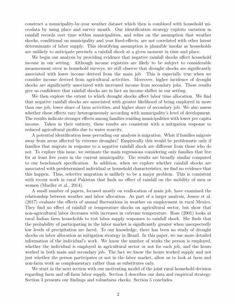
A consolidated body of research suggests that the incidence of extreme weather events, suchas droughts and floods, will rise in the coming century as a result of increased global averagetemperature (Coates et al., 2014; IPCC, 2013). The economic costs of these climate-relatedextreme events may be substantial and far-reaching. Much of the discussion in literature hasfocused on the direct impacts of extreme weather events on health, agriculture, and income.1

However, increasing attention is being paid to the mechanisms underlying these relationships.One intriguing question is whether families adopt income mitigation strategies in response toextreme weather events. While previous studies provide strong evidence that droughts andfloods can have an immediate effect on rural income, the extent to which families adjust laborsupply to mitigate these effects has been very little investigated.2 Documenting the quantitativeimportance of these labor supply and other behavioral household responses is crucial for guidingthe targeting of policies intended to mitigate the adverse consequences of climate change.

Extreme weather events can have in particular important effects on time allocation of la-bor. In context where irrigation and genetically improved seed are unavailable, rainfall shocksare likely to negatively affect agricultural productivity, most notably causing lower yields ofsubsistence crops and reduce income from cash crops. As a result, engaging in agriculturalactivities become less attractive and household should rise the supply of non-agricultural workto hedge against declining agricultural profitability and smoothing consumption. Therefore,off-farm income plays a significant role in rural households by reducing income volatility.

Understanding the labor supply responses to weather shocks is particularly relevant in de-veloping countries. Since these countries are located in areas that are warmer, they are expectedto experience a disproportionate share of extreme weather events in the future due to climatechange. Moreover, these countries have limited social safety nets and weak institutions, sohouseholds do not have access to the portfolio of adaptation strategies or avoidance behaviorsoften available in more developed countries.

In this paper, we provide empirical evidence on the relationship between rainfall shocksand household’s labor allocation in the Northeast Brazilian context. We believe that focuson Northeastern Brazil provides a compelling setting to investigate this question. First, itis the driest Brazilian region and it has long been subject to harsh climatic conditions, withrecurrent events of drought and rising temperatures, leading to further enhance evaporation andreduce water availability (Ab’Saber, 1999; Marengo, 2009). Second, one of the most populatedsemi-arid area of the world is localized in Brazilian Northeast, where more than 10 millioninhabitants are located in rural areas. For a huge fraction of this population collecting waterfor consumption, hygiene, and agricultural production is a daily task that demands energyand resources. Lack of adequate access to water also increases the susceptibility to climaticshocks associated with fluctuations in rainfall (Ab’Saber, 1999; Cirilo, 2008; Insa/MCTI, 2014;Rocha and Soares, 2015). Furthermore, half of all Brazilian rural dwellers and family farmingestablishments are in Northeast. Almost all of the total area sown in the region is rainfed.Only 2 percent of net area is irrigated.3 Therefore, we would expect rainfall to be an importantdriver of agricultural productivity and household income.

We make use of high frequency gridded information on precipitation and temperature to

1See Barreca (2012), Barrios et al. (2008), Blakeslee and Fishman (2017), Deschenes and Greenstone (2007),Jayachandran (2006), Rocha and Soares (2015), and Zander et al. (2015).

2See Jessoe et al. (2017) and Rose (2001).3These information are based on the Brazilian Agricultural Census 2006.

1

construct a municipality-by-year weather dataset which then is combined with household mi-crodata by using place and survey month. Our identification strategy exploits variation inrainfall records over time within municipalities, and relies on the assumption that weathershocks, conditional on municipality and year fixed-effects, are not correlated with other latentdeterminants of labor supply. This identifying assumption is plausible insofar as householdsare unlikely to anticipate precisely a rainfall shock at a given moment in time and place.

We begin our analysis by providing evidence that negative rainfall shocks affect householdincome in our setting. Although income registries are likely to be subject to considerablemeasurement error in household surveys, we still observe that drought shocks are significantlyassociated with lower income derived from the main job. This is especially true when weconsider income derived from agricultural activities. Moreover, higher incidence of droughtshocks are significantly associated with increased income from secondary jobs. These resultsgive us confidence that rainfall shocks are in fact an income shifter in our setting.

We then explore the extent to which drought shocks affect labor time allocation. We findthat negative rainfall shocks are associated with greater likelihood of being employed in morethan one job, lower share of farm activities, and higher share of secondary job. We also assesswhether these effects vary heterogeneously according with municipality’s level of development.The results indicate stronger effects among families residing municipalities with lower per capitaincome. Taken in their entirety, these results are consistent with a mitigation response toreduced agricultural profits due to water scarcity.

A potential identification issue pervading our analysis is migration. What if families migrateaway from areas affected by extreme droughts? Empirically this would be problematic only iffamilies that migrate in response to a negative rainfall shock are different from those who donot. To explore this issue, we estimate the main regressions considering only families that livefor at least five years in the current municipality. The results are broadly similar comparedto our benchmark specification. In addition, when we explore whether rainfall shocks areassociated with predetermined individual or household characteristics, we find no evidence thatthis happen. Thus, selective migration is unlikely to be a major problem. This is consistentwith recent work in rural Pakistan that finds no effect of rainfall on the mobility of men orwomen (Mueller et al., 2014).

A small number of papers, focused mostly on reallocation of main job, have examined therelationship between weather and labor allocation. As part of a larger analysis, Jessoe et al.(2017) evaluate the effects of annual fluctuations in weather on employment in rural Mexico.They find no effect of rainfall or temperature shocks on agricultural sector, but show thatnon-agricultural labor decreases with increases in extreme temperature. Rose (2001) looks atrural Indian farm households to test labor supply responses to rainfall shock. She finds thatthe probability of participating in the labor market is significantly greater when unexpectedlylow levels of precipitation are faced. To our knowledge, there has been no study of droughtshocks on labor allocation as mitigation strategy in Brazil. In this paper, we use more detailedinformation of the individual’s work. We know the number of works the person is employed,whether the individual is employed in agricultural sector or not for each job, and the hoursworked in both main and secondary job. The fact we know the hours worked supply and notjust whether the person participates or not in the labor market, allow us to look at farm andnon-farm work as complementary rather than as substitutes only.

We start in the next section with our motivating model of the joint rural household decisionregarding farm and off-farm labor supply. Section 3 describes our data and empirical strategy.Section 4 presents our findings and robustness checks. Section 5 concludes.

2

2 A model of rural household labor

We developed a simple model of the joint rural household decision regarding farm and off-farmlabor supply. The household decides to allocate the time T among three activities: leisure(lz), farm labor (lfarm) and off-farm labor (loff ), such that T = lz + lfarm + loff . Let c beconsumption. The rural household utility function U(c, lz) is concave and twice differentiable.The total utility function of the rural household is:

U(c, lz) = u(c) + αlz (1)

Let w denote the off-farm wage and, since the agricultural household is a price-taker in allmarkets (Singh, Squire and Strauss, 1986), we assume that w is determined exogenously. So,household will be paid wloff for time spent working in off-farm labor. Let π be the revenue fromagriculture, which is given by agricultural production. Agricultural production is determined bythe amount of farm labor, weather shocks, and fixed capital and land. It may be representedby the production function q(lfarm, R,K), where lfarm is the quantity of labor allocated tofarm activities, R the weather shock, and K is capital and land.4 R is a random variablethat affects farm profits, a higher value of R indicates better weather. It could be defined asthe deviation between the total rainfall in given moment of time and the historical averagerainfall.5 Literature shows that rural Northeastern Brazil turns positive rainfall shocks intounequivocally beneficial events, enabling us to assume that ∂q

∂R> 0.6 Total rural household

income is given by the sum of farm revenue and off-farm income, and it may be represented byI = Pq(lfarm, R,K) + wloff . Thus, consumption will be

c = I (2)

c = Pq(lfarm, R,K) + wloff (3)

The time allocated to leisure is expressed by lz = T − lfarm − loff . Thus, we can substitutethis into the maximization problem to get

maxlfarm,loff

U[Pq(lfarm, R,K) + wloff , T − lfarm − loff

](4)

We consider the case where rural households allocate time for both farm and off-farm ac-tivities. In this case, the first order conditions of the optimization problem (4) are given by

u′(c)

(P

∂q

∂lfarm

)− α = 0 (5)

u′(c)w − α = 0 (6)

where u′(c) is the marginal utility of the consume and α is the marginal utility of leisure.From conditions (5) and (6), one may verify that(

P∂q

∂lfarm

)= w (7)

4In general, we assume that ∂q∂lfarm > 0, ∂2q

∂2lfarm < 0, and ∂2q∂lfarm∂R

> 05Rainfall deviations below the historical average characterizes a negative shock, whereas deviations above

the historical average settles a positive shock.6See Rocha and Soares (2015).

3

Condition (7) indicates that, on optimum, the farm wage is equal to the wage paid by off-farm activities. To ensure a globally concave objective function, and thus, a unique optimum,we assume that:[

u′′(c)

(P

∂q

∂lfarm

)2

+ P∂2q

∂2lfarmu′(c)

]u′′(c)w2 >

[u′′(c)w

(P

∂q

∂lfarm

)]2(8)

We are interested in the effect that weather shocks have on the optimal level of both farmand off-farm labor. That is, how would we expect an adverse weather shock to affect the ruralhousehold labor decision? They would use off-farm labor as a mitigation strategy to weathershocks? These questions lead us to our two testable hypothesis:

Proposition 1. Negative rainfall shocks decrease household farm labor supply.

Proof. It follows from the first order condition:

∂lfarm

∂R∼=

(+)︷︸︸︷−u′′(c)w2u′(c)P

(∂lfarm

∂R

)(9)

�

Farm work has a positive relationship with R. In other words, an increase (reduction) in Rimplies in increasing (decreasing) farm labor. In this model, there is only one way that weathershocks affect the choice of farm work. When a drought is faced, the marginal productivity ofagricultural labor will reduce, which implies a diminishing in the return of farm labor. Thereby,agricultural activities become less attractive. Household will allocate less time to farm labor,thus reducing lfarm. However, positive rainfall shocks increase the benefit to farm working,agricultural wage rises and household will increase farm labor supply.

Proposition 2. Negative rainfall shocks increase household non-agricultural labor supply.

Proof. From the first order condition, we can derivate the effect of weather shocks on theoptimal choice of off-farm working:

∂loff

∂R∼=

(−)︷︸︸︷−u′′(c)P ∂q

∂Rwu′(c)P

∂2q

∂2lfarm+ u′′(c)w2u′(c)P

∂2q

∂lfarm∂R(10)

�

Weather shock has two effects on the optimal level of off-farm labor. First, a droughtdecreases both farmland productivity and the value of agricultural work, which affect the benefitof time spent in farm labor. Thus, off-farm labor becomes more attractive, and household willincrease loff . Second, droughts decreases the value of marginal productivity of farm labor.Since the marginal return associated to off-farm activities is higher, the household could chooseoff-farm labor above the optimal level, leading to rising the total income, and mitigating theshocks effect.

4

3 Data and Empirical Strategy

3.1 Household data

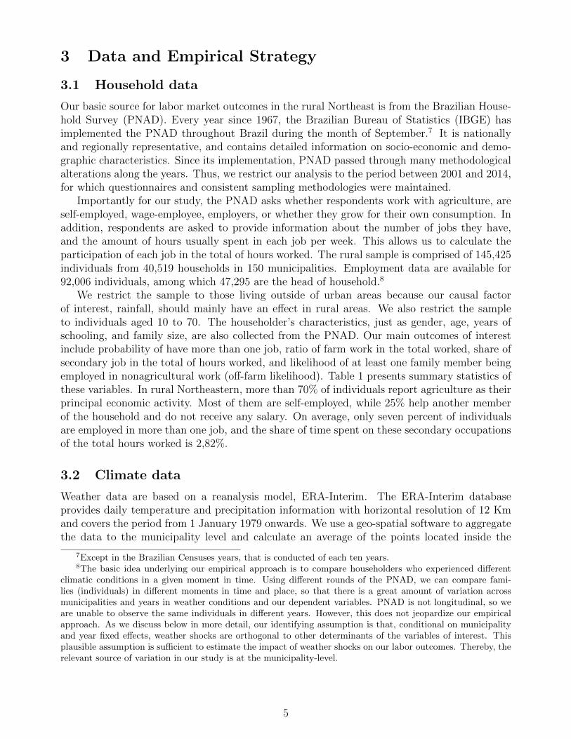
Our basic source for labor market outcomes in the rural Northeast is from the Brazilian House-hold Survey (PNAD). Every year since 1967, the Brazilian Bureau of Statistics (IBGE) hasimplemented the PNAD throughout Brazil during the month of September.7 It is nationallyand regionally representative, and contains detailed information on socio-economic and demo-graphic characteristics. Since its implementation, PNAD passed through many methodologicalalterations along the years. Thus, we restrict our analysis to the period between 2001 and 2014,for which questionnaires and consistent sampling methodologies were maintained.

Importantly for our study, the PNAD asks whether respondents work with agriculture, areself-employed, wage-employee, employers, or whether they grow for their own consumption. Inaddition, respondents are asked to provide information about the number of jobs they have,and the amount of hours usually spent in each job per week. This allows us to calculate theparticipation of each job in the total of hours worked. The rural sample is comprised of 145,425individuals from 40,519 households in 150 municipalities. Employment data are available for92,006 individuals, among which 47,295 are the head of household.8

We restrict the sample to those living outside of urban areas because our causal factorof interest, rainfall, should mainly have an effect in rural areas. We also restrict the sampleto individuals aged 10 to 70. The householder’s characteristics, just as gender, age, years ofschooling, and family size, are also collected from the PNAD. Our main outcomes of interestinclude probability of have more than one job, ratio of farm work in the total worked, share ofsecondary job in the total of hours worked, and likelihood of at least one family member beingemployed in nonagricultural work (off-farm likelihood). Table 1 presents summary statistics ofthese variables. In rural Northeastern, more than 70% of individuals report agriculture as theirprincipal economic activity. Most of them are self-employed, while 25% help another memberof the household and do not receive any salary. On average, only seven percent of individualsare employed in more than one job, and the share of time spent on these secondary occupationsof the total hours worked is 2,82%.

3.2 Climate data

Weather data are based on a reanalysis model, ERA-Interim. The ERA-Interim databaseprovides daily temperature and precipitation information with horizontal resolution of 12 Kmand covers the period from 1 January 1979 onwards. We use a geo-spatial software to aggregatethe data to the municipality level and calculate an average of the points located inside the

7Except in the Brazilian Censuses years, that is conducted of each ten years.8The basic idea underlying our empirical approach is to compare householders who experienced different

climatic conditions in a given moment in time. Using different rounds of the PNAD, we can compare fami-lies (individuals) in different moments in time and place, so that there is a great amount of variation acrossmunicipalities and years in weather conditions and our dependent variables. PNAD is not longitudinal, so weare unable to observe the same individuals in different years. However, this does not jeopardize our empiricalapproach. As we discuss below in more detail, our identifying assumption is that, conditional on municipalityand year fixed effects, weather shocks are orthogonal to other determinants of the variables of interest. Thisplausible assumption is sufficient to estimate the impact of weather shocks on our labor outcomes. Thereby, therelevant source of variation in our study is at the municipality-level.

5

municipality limits.9 We make use of this daily data in order to construct drought shockmeasures.

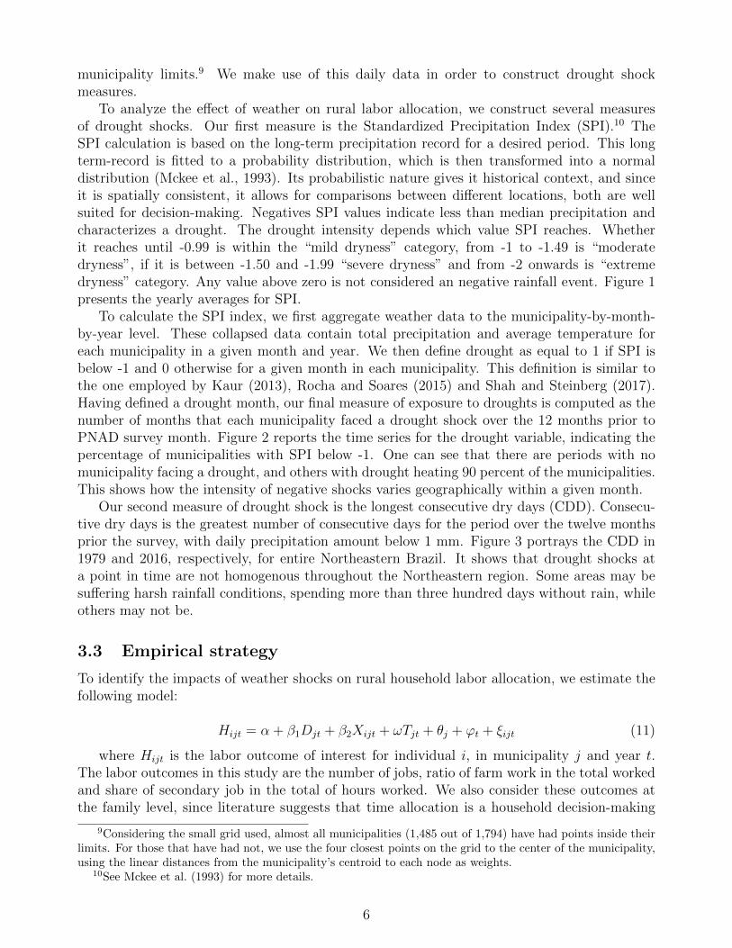
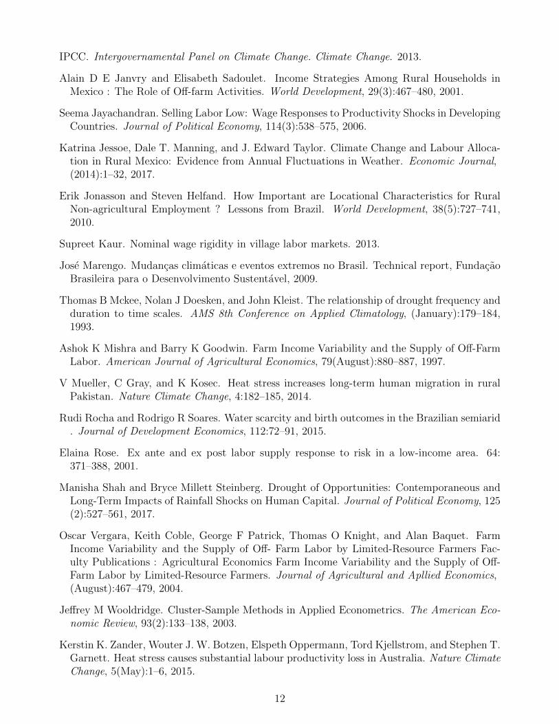
To analyze the effect of weather on rural labor allocation, we construct several measuresof drought shocks. Our first measure is the Standardized Precipitation Index (SPI).10 TheSPI calculation is based on the long-term precipitation record for a desired period. This longterm-record is fitted to a probability distribution, which is then transformed into a normaldistribution (Mckee et al., 1993). Its probabilistic nature gives it historical context, and sinceit is spatially consistent, it allows for comparisons between different locations, both are wellsuited for decision-making. Negatives SPI values indicate less than median precipitation andcharacterizes a drought. The drought intensity depends which value SPI reaches. Whetherit reaches until -0.99 is within the “mild dryness” category, from -1 to -1.49 is “moderatedryness”, if it is between -1.50 and -1.99 “severe dryness” and from -2 onwards is “extremedryness” category. Any value above zero is not considered an negative rainfall event. Figure 1presents the yearly averages for SPI.

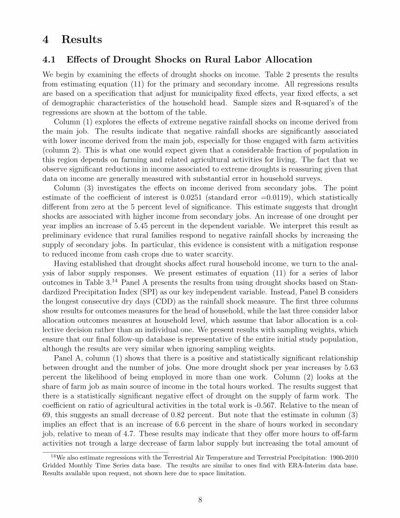
To calculate the SPI index, we first aggregate weather data to the municipality-by-month-by-year level. These collapsed data contain total precipitation and average temperature foreach municipality in a given month and year. We then define drought as equal to 1 if SPI isbelow -1 and 0 otherwise for a given month in each municipality. This definition is similar tothe one employed by Kaur (2013), Rocha and Soares (2015) and Shah and Steinberg (2017).Having defined a drought month, our final measure of exposure to droughts is computed as thenumber of months that each municipality faced a drought shock over the 12 months prior toPNAD survey month. Figure 2 reports the time series for the drought variable, indicating thepercentage of municipalities with SPI below -1. One can see that there are periods with nomunicipality facing a drought, and others with drought heating 90 percent of the municipalities.This shows how the intensity of negative shocks varies geographically within a given month.

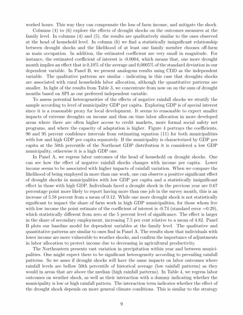
Our second measure of drought shock is the longest consecutive dry days (CDD). Consecu-tive dry days is the greatest number of consecutive days for the period over the twelve monthsprior the survey, with daily precipitation amount below 1 mm. Figure 3 portrays the CDD in1979 and 2016, respectively, for entire Northeastern Brazil. It shows that drought shocks ata point in time are not homogenous throughout the Northeastern region. Some areas may besuffering harsh rainfall conditions, spending more than three hundred days without rain, whileothers may not be.

3.3 Empirical strategy

To identify the impacts of weather shocks on rural household labor allocation, we estimate thefollowing model:

Hijt = α + β1Djt + β2Xijt + ωTjt + θj + ϕt + ξijt (11)

where Hijt is the labor outcome of interest for individual i, in municipality j and year t.The labor outcomes in this study are the number of jobs, ratio of farm work in the total workedand share of secondary job in the total of hours worked. We also consider these outcomes atthe family level, since literature suggests that time allocation is a household decision-making

9Considering the small grid used, almost all municipalities (1,485 out of 1,794) have had points inside theirlimits. For those that have had not, we use the four closest points on the grid to the center of the municipality,using the linear distances from the municipality’s centroid to each node as weights.

10See Mckee et al. (1993) for more details.

6

process rather than an individual one.11 In particular, we consider a dummy indicating whetherat least one household member is mainly employed in the off-farm market. Djt is a droughtshock measure (either the longest consecutive dry days in the 12 months prior to survey orthe number of drought months in the same period) in year t and municipality j, which is ourregressor of interest. We also control for householder’s characteristics, just as gender, age, raceand family size, by including the vector Xijt. Tjt is the average temperature in the municipalityj, on year t.12

The model includes municipality fixed effects (θj), which absorb any unobservable timeinvariant factors, including initial conditions and persistent municipality characteristics suchas geography. Year fixed effects (ϕt) capture aggregate shocks impacting all Northeast region,including aggregated demand shocks, and regional policies and programs. Standard errorsare clustered at the municipality level to account for serial correlation (Bertrand et al., 2004;Wooldridge, 2003).13

The parameter of interest β1 measures the relationship between rainfall shocks and labormarket outcomes. The identifying assumption underlying this statistical approach is that, con-ditional on municipality and year fixed effects, there are not determinants omitted of labor mar-ket outcomes correlated with the incidence of weather shocks. This seems plausible, given thatthe occurrence of extreme weather event at a given moment in time and place is unpredictable.Thus, our approach exploits arguably random fluctuations in rainfall from municipality-specificdeviations in long-term rainfall after controlling for all seasonal factors and common shocks toall municipalities.

Although much of the variation in rainfall shocks over time within municipalities appearsto be idiosyncratic, an identification issue could arise when following this specification. Inparticular, one may be concerned whether rural families respond migrating away from areasaffected by extreme droughts. This would be problematic only if families that migrate inresponse to an extreme rainfall shock are different to families who do not. We address thisissue in two way. First, we estimate the main regressions considering only families that live forat least five years in the current municipality. If regression results are similar to the ones derivedfrom the baseline, we would be more confident that selective migration is unlikely to be a majorissue. Second, we explore whether rainfall shocks are associated with predetermined individualor household characteristics. If different families are more likely to respond to rainfall shocksby migrating, one would expect to see significant effects of rainfall shocks on predeterminedcharacteristics. As we shown below, there is very little evidence that this is the case. Perhaps,this is not very surprisingly, given we are exploiting temporary deviations in rainfall from thehistorical norm. Migration is likely to be a more salient issue in the case of prolonged andpermanent changes in rainfall.

11See, for example,Demurger et al. (2010), Ellis (2000), Janvry and Sadoulet (2001), Jonasson and Helfand(2010), Mishra and Goodwin (1997), and Vergara et al. (2004).

12We also control for bins of temperature in order to capture its nonlinear impacts. The results were thesame, with temperature presenting no statistical significance.

13We also compute standard errors clustered at micro and macro-region level. Statistical significance is thesame.

7

4 Results

4.1 Effects of Drought Shocks on Rural Labor Allocation

We begin by examining the effects of drought shocks on income. Table 2 presents the resultsfrom estimating equation (11) for the primary and secondary income. All regressions resultsare based on a specification that adjust for municipality fixed effects, year fixed effects, a setof demographic characteristics of the household head. Sample sizes and R-squared’s of theregressions are shown at the bottom of the table.

Column (1) explores the effects of extreme negative rainfall shocks on income derived fromthe main job. The results indicate that negative rainfall shocks are significantly associatedwith lower income derived from the main job, especially for those engaged with farm activities(column 2). This is what one would expect given that a considerable fraction of population inthis region depends on farming and related agricultural activities for living. The fact that weobserve significant reductions in income associated to extreme droughts is reassuring given thatdata on income are generally measured with substantial error in household surveys.

Column (3) investigates the effects on income derived from secondary jobs. The pointestimate of the coefficient of interest is 0.0251 (standard error =0.0119), which statisticallydifferent from zero at the 5 percent level of significance. This estimate suggests that droughtshocks are associated with higher income from secondary jobs. An increase of one drought peryear implies an increase of 5.45 percent in the dependent variable. We interpret this result aspreliminary evidence that rural families respond to negative rainfall shocks by increasing thesupply of secondary jobs. In particular, this evidence is consistent with a mitigation responseto reduced income from cash crops due to water scarcity.

Having established that drought shocks affect rural household income, we turn to the anal-ysis of labor supply responses. We present estimates of equation (11) for a series of laboroutcomes in Table 3.14 Panel A presents the results from using drought shocks based on Stan-dardized Precipitation Index (SPI) as our key independent variable. Instead, Panel B considersthe longest consecutive dry days (CDD) as the rainfall shock measure. The first three columnsshow results for outcomes measures for the head of household, while the last three consider laborallocation outcomes measures at household level, which assume that labor allocation is a col-lective decision rather than an individual one. We present results with sampling weights, whichensure that our final follow-up database is representative of the entire initial study population,although the results are very similar when ignoring sampling weights.

Panel A, column (1) shows that there is a positive and statistically significant relationshipbetween drought and the number of jobs. One more drought shock per year increases by 5.63percent the likelihood of being employed in more than one work. Column (2) looks at theshare of farm job as main source of income in the total hours worked. The results suggest thatthere is a statistically significant negative effect of drought on the supply of farm work. Thecoefficient on ratio of agricultural activities in the total work is -0.567. Relative to the mean of69, this suggests an small decrease of 0.82 percent. But note that the estimate in column (3)implies an effect that is an increase of 6.6 percent in the share of hours worked in secondaryjob, relative to mean of 4.7. These results may indicate that they offer more hours to off-farmactivities not trough a large decrease of farm labor supply but increasing the total amount of

14We also estimate regressions with the Terrestrial Air Temperature and Terrestrial Precipitation: 1900-2010Gridded Monthly Time Series data base. The results are similar to ones find with ERA-Interim data base.Results available upon request, not shown here due to space limitation.

8

worked hours. This way they can compensate the loss of farm income, and mitigate the shock.Columns (4) to (6) explore the effects of drought shocks on the outcomes measures at the

family level. In columns (4) and (5), the results are qualitatively similar to the ones observedat the head of household level. In column (6) we find a statistically insignificant relationshipbetween drought shocks and the likelihood of at least one family member chooses off-farmas main occupation. In addition, the estimated coefficient are very small in magnitude. Forinstance, the estimated coefficient of interest is -0.0004, which means that, one more droughtmonth implies an effect that is 0,10% of the average and 0,0005% of the standard deviation in ourdependent variable. In Panel B, we present analogous results using CDD as the independentvariable. The qualitative patterns are similar - indicating in this case that droughts shocksare associated with rural households labor allocation, although the quantitative patterns aresmaller. In light of the results from Table 3, we concentrate from now on on the sum of droughtmonths based on SPI as our preferred independent variable.

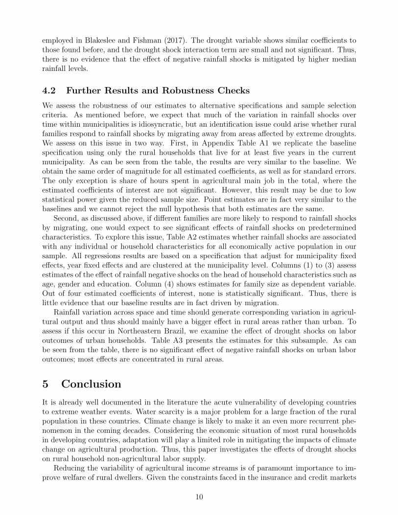
To assess potential heterogeneities of the effects of negative rainfall shocks we stratify thesample according to level of municipality GDP per capita. Exploring GDP is of special interestsince it is a reasonable proxy for local development. It seems to reasonable to expect smallerimpacts of extreme droughts on income and thus on time labor allocation in more developedareas where there are often higher access to credit markets, more formal social safety netprograms, and where the capacity of adaptation is higher. Figure 4 portrays the coefficients,90 and 95 percent confidence intervals from estimating equation (11) for both municipalitieswith low and high GDP per capita separately. If the municipality is characterized by GDP percapita at the 50th percentile of the Northeast GDP distribution it is considered a low GDPmunicipality, otherwise it is a high GDP one.

In Panel A, we regress labor outcomes of the head of household on drought shocks. Onecan see how the effect of negative rainfall shocks changes with income per capita. Lowerincome seems to be associated with higher impacts of rainfall variation. When we compare thelikelihood of being employed in more than one work, one can observe a positive significant effectof drought shocks in municipalities with low GDP per capita and a statistically insignificanteffect in those with high GDP. Individuals faced a drought shock in the previous year are 0.67percentage point more likely to report having more than one job in the survey month, this is anincrease of 5.58 percent from a mean of 0.12. While one more drought shock is not statisticallysignificant to impact the share of farm work in high GDP municipalities, for those whom livewith low income the point estimate of the coefficient of interest is -0.74 (standard error =0.29),which statistically different from zero at the 5 percent level of significance. The effect is largerin the share of secondary employment, increasing 7.5 per cent relative to a mean of 4.82. PanelB plots our baseline model for dependent variables at the family level. The qualitative andquantitative patterns are similar to ones find in Panel A. The results show that individuals withlower income are more vulnerable to weather shocks, and confirm the importance of adjustmentsin labor allocation to protect income due to decreasing in agricultural productivity.

The Northeastern presents vast variation in precipitation within year and between munici-palities. One might expect there to be significant heterogeneity according to prevailing rainfallpatterns. So we asses if drought shocks will have the same impacts on labor outcomes whererainfall levels are bellow 50th percentile of historical average (low rainfall patterns) as theywould in areas that are above the median (high rainfall patterns). In Table 4, we regress laboroutcomes on weather shock, as well as their interaction with a dummy indicating whether themunicipality is low or high rainfall pattern. The interaction term indicates whether the effect ofthe drought shock depends on more general climate conditions. This is similar to the strategy

9

employed in Blakeslee and Fishman (2017). The drought variable shows similar coefficients tothose found before, and the drought shock interaction term are small and not significant. Thus,there is no evidence that the effect of negative rainfall shocks is mitigated by higher medianrainfall levels.

4.2 Further Results and Robustness Checks

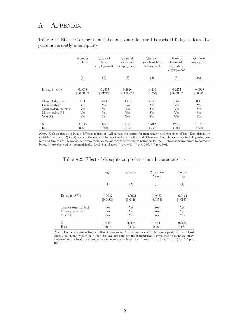
We assess the robustness of our estimates to alternative specifications and sample selectioncriteria. As mentioned before, we expect that much of the variation in rainfall shocks overtime within municipalities is idiosyncratic, but an identification issue could arise whether ruralfamilies respond to rainfall shocks by migrating away from areas affected by extreme droughts.We assess on this issue in two way. First, in Appendix Table A1 we replicate the baselinespecification using only the rural households that live for at least five years in the currentmunicipality. As can be seen from the table, the results are very similar to the baseline. Weobtain the same order of magnitude for all estimated coefficients, as well as for standard errors.The only exception is share of hours spent in agricultural main job in the total, where theestimated coefficients of interest are not significant. However, this result may be due to lowstatistical power given the reduced sample size. Point estimates are in fact very similar to thebaselines and we cannot reject the null hypothesis that both estimates are the same.

Second, as discussed above, if different families are more likely to respond to rainfall shocksby migrating, one would expect to see significant effects of rainfall shocks on predeterminedcharacteristics. To explore this issue, Table A2 estimates whether rainfall shocks are associatedwith any individual or household characteristics for all economically active population in oursample. All regressions results are based on a specification that adjust for municipality fixedeffects, year fixed effects and are clustered at the municipality level. Columns (1) to (3) assessestimates of the effect of rainfall negative shocks on the head of household characteristics such asage, gender and education. Column (4) shows estimates for family size as dependent variable.Out of four estimated coefficients of interest, none is statistically significant. Thus, there islittle evidence that our baseline results are in fact driven by migration.

Rainfall variation across space and time should generate corresponding variation in agricul-tural output and thus should mainly have a bigger effect in rural areas rather than urban. Toassess if this occur in Northeastern Brazil, we examine the effect of drought shocks on laboroutcomes of urban households. Table A3 presents the estimates for this subsample. As canbe seen from the table, there is no significant effect of negative rainfall shocks on urban laboroutcomes; most effects are concentrated in rural areas.

5 Conclusion

It is already well documented in the literature the acute vulnerability of developing countriesto extreme weather events. Water scarcity is a major problem for a large fraction of the ruralpopulation in these countries. Climate change is likely to make it an even more recurrent phe-nomenon in the coming decades. Considering the economic situation of most rural householdsin developing countries, adaptation will play a limited role in mitigating the impacts of climatechange on agricultural production. Thus, this paper investigates the effects of drought shockson rural household non-agricultural labor supply.

Reducing the variability of agricultural income streams is of paramount importance to im-prove welfare of rural dwellers. Given the constraints faced in the insurance and credit markets

10

by most rural families in developing countries, labor reallocation can be one of the main chan-nels by which poor rural households mitigate negative rainfall shocks. Engaging in off-farmlabor market might help households to smooth income.

The strategy outlined here presents evidence of a relationship between negative rainfallevents and labor time reallocation. We find that drought shocks are significantly associatedwith lower income derived from the main job. This is especially true when we consider incomederived from farm activities. Moreover, higher incidence of drought shocks are significantlyassociated with increased income from secondary jobs. Our results show that droughts affectnegatively hours spent on farm work, whereas lead to increased supply of non-agriculturaljob. One can also observe stronger effects among families residing in municipalities with lowerper capita income. Taken together, our findings suggest that families adjust labor supply tomitigate the income effects of water scarcity.

References

Aziz Nacib Ab’Saber. Sertoes e sertanejos: uma geografia humana sofrida. Estudos Avancados,13(36):5–59, 1999.

Alan I. Barreca. Climate change, humidity, and mortality in the United States. Journal ofEnvironmental Economics and Management, 63(1):19–34, 2012.

Salvador Barrios, Ouattara Bazoumana, and Eric Strobl. The impact of climatic change onagricultural production: Is it different for Africa? Food Policy, 33(4):287–298, 2008.

Marianne Bertrand, Esther Duflo, and Sendhil Mullainathan. How Much Should We TrustDifferences-in-Differences Estimates ? The Quarterly Journal of Economics, 119(1):249–275,2004.

David S Blakeslee and Ram Fishman. Weather Shocks , Agriculture , and Crime : Evidencefrom India. 2017.

Jose Almir Cirilo. Polıticas publicas de recursos hıdricos para o semi-arido. Estudos Avancados,22(63):61–82, 2008.

Lucinda Coates, Katharine Haynes, James O’Brien, John McAneney, and Felipe Dimer DeOliveira. Exploring 167 years of vulnerability: An examination of extreme heat events inAustralia 1844-2010. Environmental Science and Policy, 42:33–44, 2014.

Sylvie Demurger, Martin Fournier, and Weiyong Yang. Rural households ’ decisions towardsincome diversi fi cation : Evidence from a township in northern China. China EconomicReview, 21:S32–S44, 2010.

Olivier Deschenes and Michael Greenstone. The economic impacts of climate change: Evidencefrom agricultural output and random fuctuations in weather. American Economic Review,97(1):354–385, 2007.

Frank Ellis. The Determinants of Rural Livelihood Diversification in Developing Countries.Journal of Agricultural Economics, 51(2):289–302, 2000.

Insa/MCTI. Populacao do Semiarido brasileiro ultrapassa 23,5 milhoes de habitantes, 2014.

11

IPCC. Intergovernamental Panel on Climate Change. Climate Change. 2013.

Alain D E Janvry and Elisabeth Sadoulet. Income Strategies Among Rural Households inMexico : The Role of Off-farm Activities. World Development, 29(3):467–480, 2001.

Seema Jayachandran. Selling Labor Low: Wage Responses to Productivity Shocks in DevelopingCountries. Journal of Political Economy, 114(3):538–575, 2006.

Katrina Jessoe, Dale T. Manning, and J. Edward Taylor. Climate Change and Labour Alloca-tion in Rural Mexico: Evidence from Annual Fluctuations in Weather. Economic Journal,(2014):1–32, 2017.

Erik Jonasson and Steven Helfand. How Important are Locational Characteristics for RuralNon-agricultural Employment ? Lessons from Brazil. World Development, 38(5):727–741,2010.

Supreet Kaur. Nominal wage rigidity in village labor markets. 2013.

Jose Marengo. Mudancas climaticas e eventos extremos no Brasil. Technical report, FundacaoBrasileira para o Desenvolvimento Sustentavel, 2009.

Thomas B Mckee, Nolan J Doesken, and John Kleist. The relationship of drought frequency andduration to time scales. AMS 8th Conference on Applied Climatology, (January):179–184,1993.

Ashok K Mishra and Barry K Goodwin. Farm Income Variability and the Supply of Off-FarmLabor. American Journal of Agricultural Economics, 79(August):880–887, 1997.

V Mueller, C Gray, and K Kosec. Heat stress increases long-term human migration in ruralPakistan. Nature Climate Change, 4:182–185, 2014.

Rudi Rocha and Rodrigo R Soares. Water scarcity and birth outcomes in the Brazilian semiarid. Journal of Development Economics, 112:72–91, 2015.

Elaina Rose. Ex ante and ex post labor supply response to risk in a low-income area. 64:371–388, 2001.

Manisha Shah and Bryce Millett Steinberg. Drought of Opportunities: Contemporaneous andLong-Term Impacts of Rainfall Shocks on Human Capital. Journal of Political Economy, 125(2):527–561, 2017.

Oscar Vergara, Keith Coble, George F Patrick, Thomas O Knight, and Alan Baquet. FarmIncome Variability and the Supply of Off- Farm Labor by Limited-Resource Farmers Fac-ulty Publications : Agricultural Economics Farm Income Variability and the Supply of Off-Farm Labor by Limited-Resource Farmers. Journal of Agricultural and Apllied Economics,(August):467–479, 2004.

Jeffrey M Wooldridge. Cluster-Sample Methods in Applied Econometrics. The American Eco-nomic Review, 93(2):133–138, 2003.

Kerstin K. Zander, Wouter J. W. Botzen, Elspeth Oppermann, Tord Kjellstrom, and Stephen T.Garnett. Heat stress causes substantial labour productivity loss in Australia. Nature ClimateChange, 5(May):1–6, 2015.

12

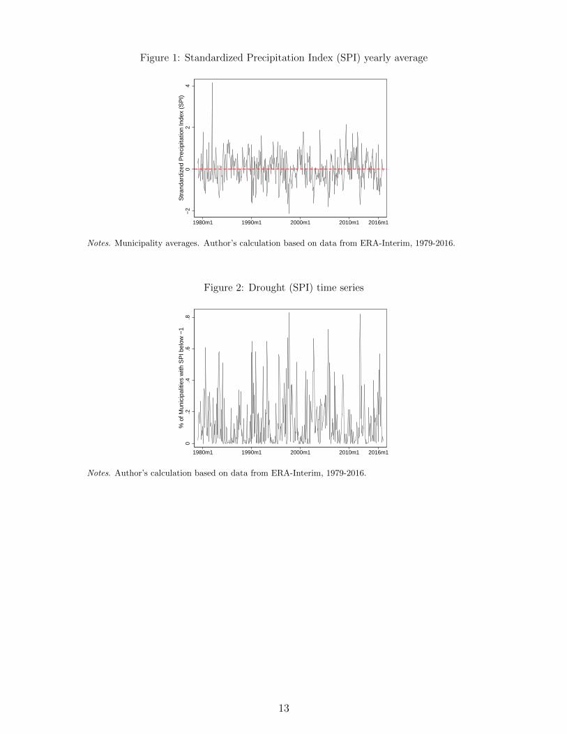
Figure 1: Standardized Precipitation Index (SPI) yearly average

−2

02

4S

tran

dard

ized

Pre

cipi

tatio

n In

dex

(SP

I)

1980m1 1990m1 2000m1 2010m1 2016m1

Notes. Municipality averages. Author’s calculation based on data from ERA-Interim, 1979-2016.

Figure 2: Drought (SPI) time series

0.2

.4.6

.8%

of M

unic

ipal

ities

with

SP

I bel

ow −

1

1980m1 1990m1 2000m1 2010m1 2016m1

Notes. Author’s calculation based on data from ERA-Interim, 1979-2016.

13

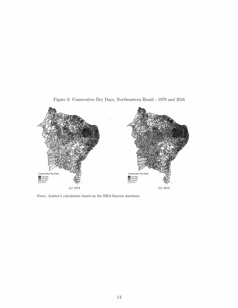
Figure 3: Consecutive Dry Days, Northeastern Brazil - 1979 and 2016

Consecutive Dry Days(200,365](100,200](50,100][0,50]

(a) 1979

Consecutive Dry Days(200,365](100,200](50,100][0,50]

(b) 2016

Notes. Author’s calculation based on the ERA-Interim database.

14

Figure 4: Effects of drought shocks on labor outcomes by GDP per capita level

Drought (SPI)

Drought (SPI)

0 .005 .01 .015 −1.5 −1 −.5 0 .5

0 .2 .4 .6

Number of Jobs Share of Farm Employment

Share of Secondary Employment

Low GDP High GDP

(a) Individual level

Drought (SPI)

Drought (SPI)

−1.5 −1 −.5 0 .5 0 .2 .4 .6

−.01 −.005 0 .005 .01

Share of Farm Employment Share of Secondary Employment

Off−farm Employment

Low GDP High GDP

(b) Family level

Notes. This is an event-study created by regressing labor outcomes on drought shocks and on a set ofcontrols. The controls include municipality and year fixed effects, individual and household characteristicssuch as gender, age, race and family size. Temperature control include the average temperature atmunicipality level. Robust standard errors (reported in brackets) are clustered at the municipality level.

15

Table 1: Summary statistics

Mean Std. Min Max Ndeviation

Demographic characteristics:Gender 0.52 0.5 0 1 145,425Age 33.9 18.37 10 70 145,425Education years 4.81 3.62 1 17 145,425Number of household members 4.46 2.08 1 17 145,425

Employment characteristics:More than one job 0.07 0.25 0 1 92,006Farm work as main 0.73 0.44 0 1 92,006Share of farm job 70.43 44.38 0 100 92,006Share of secondary job 2.82 11 0 97.82 92,006Off-farm (likelihood) 0.42 0.49 0 1 92,006Agriculture wage job 0.22 0.41 0 1 65,790Agriculture self-employed 0.28 0.45 0 1 65,790Agriculture employer 0.02 0.13 0 1 65,790Agriculture unpaid 0.25 0.43 0 1 65,790Agriculture own consumption 0.24 0.42 0 1 65,790Off-farm wage job 0.63 0.48 0 1 26,216Off-farm self-employed 0.27 0.44 0 1 26,216Off-farm employer 0.01 0.12 0 1 26,216Off-farm unpaid 0.05 0.23 0 1 26,216

Notes. This table shows summary statistics from the PNAD.

Table 2: Effect of droughts on rural household income

Main Income Main Income Agr. Secondary Income(log) (log) (log)

(1) (2) (3)

Drought (SPI) -0.0141 -0.0193 0.0251[0.0081]* [0.0097]** [0.0119]**

Mean of dep. variable 5.4 5.17 0.46Basic controls Yes Yes YesTemperature control Yes Yes YesYear FE Yes Yes YesMunicipality FE Yes Yes Yes

N 39720 21937 39720R-sq 0.303 0.304 0.111

Notes. All outcomes are measured in log. Each coefficient is from a different regression. All regres-sions control for municipality and year fixed effects. We exclude observations in the top percentileof total income. Basic controls include gender, age, race and family size. Temperature control in-cludes the average temperature at municipality level. The number of observations differs in column(2) because it only considers households with agricultural job as main source of income. Robuststandard errors (reported in brackets) are clustered at the municipality level. Significance: * p <0.10, ** p < 0.05, *** p < 0.01.

16

Table 3: Effect of droughts on rural household labor outcomes

Number Share of Share of Share of Share of Off-farmof Jobs farm secondary household farm household employment

employement employment employment secondaryemployment

(1) (2) (3) (4) (5) (6)

Panel ADrought (SPI) 0.0062 -0.5673 0.284 -0.4492 0.2152 -0.0004

[0.0031]* [0.2570]** [0.1248]** [0.2709]* [0.0990]** [0.0029]

Panel BCDD 0.0003 -0.0267 0.01 -0.0291 0.009 0.0002

[0.0001]* [0.0179] [0.0057]* [0.0184] [0.0046]* [0.0002]

Mean of dep. var. 0.11 69.5 4.37 65.9 3.47 0.37Basic controls Yes Yes Yes Yes Yes YesTemperature control Yes Yes Yes Yes Yes YesMunicipality FE Yes Yes Yes Yes Yes YesYear FE Yes Yes Yes Yes Yes Yes

N 40006 40006 40006 42952 42952 47295R-sq 0.129 0.177 0.121 0.182 0.122 0.116

Notes. Each coefficient is from a different regression. Each panel corresponds to a different independent variable. Allregressions control for municipality and year fixed effects. Each dependent variable in columns (2) to (5) refers to theshare of the mentioned work in the total of hours worked. Basic controls include gender, age, race and family size. Tem-perature control includes the average temperature at municipality level. Robust standard errors (reported in brackets)are clustered at the municipality level. Significance: * p < 0.10, ** p < 0.05, *** p < 0.01.

Table 4: Effect of droughts on rural household labor outcomes by rainfall level



(1) (2) (3) (4) (5) (6)

Drought (SPI) 0.0075 -0.546 0.3448 -0.5214 0.2698 -0.0004[0.0038]** [0.3033]* [0.1536]** [0.3263] [0.1276]** [0.0033]

Drought × low rainfall -0.003 -0.0465 -0.1331 0.1569 -0.1185 -0.0001[0.0031] [0.2889] [0.1353] [0.3074] [0.1025] [0.0031]

Mean of dep. var. 0.11 69.5 4.37 65.9 3.47 0.37Basic controls Yes Yes Yes Yes Yes YesTemperature control Yes Yes Yes Yes Yes YesYear FE Yes Yes Yes Yes Yes YesMunicipality FE Yes Yes Yes Yes Yes Yes

N 40006 40006 40006 42952 42952 47295R-sq 0.129 0.177 0.121 0.182 0.122 0.116

Notes. Each coefficient is from a different regression. All regressions control for municipality and year fixed effects. Eachdependent variable in columns (2) to (5) refers to the share of the mentioned work in the total of hours worked. Basiccontrols include gender, age, race and family size. Temperature control includes the average temperature at municipalitylevel. Robust standard errors (reported in brackets) are clustered at the municipality level. Significance: * p < 0.10, ** p< 0.05, *** p < 0.01.

17

A Appendix

Table A.1: Effect of droughts on labor outcomes for rural household living at least fiveyears in currently municipality



(1) (2) (3) (4) (5) (6)

Drought (SPI) 0.0068 -0.2467 0.2926 -0.294 0.2254 -0.0029[0.0031]** [0.3763] [0.1189]** [0.4557] [0.0921]** [0.0046]


N 11048 11048 11048 12012 12012 13166R-sq 0.146 0.248 0.136 0.251 0.137 0.158

Notes. Each coefficient is from a different regression. All regressions control for municipality and year fixed effects. Each dependentvariable in columns (2) to (5) refers to the share of the mentioned work in the total of hours worked. Basic controls include gender, age,race and family size. Temperature control includes the average temperature at municipality level. Robust standard errors (reported inbrackets) are clustered at the municipality level. Significance: * p < 0.10, ** p < 0.05, *** p < 0.01.

Table A.2: Effect of droughts on predetermined characteristics

Age Gender Education FamilyYears Size

(1) (2) (3) (4)

Drought (SPI) -0.0227 -0.0024 -0.0032 -0.0164[0.0488] [0.0029] [0.0155] [0.0135]

Temperature control Yes Yes Yes YesMunicipality FE Yes Yes Yes YesYear FE Yes Yes Yes Yes

N 92006 92006 92006 92006R-sq 0.017 0.008 0.084 0.061

Notes. Each coefficient is from a different regression. All regressions control for municipality and year fixedeffects. Temperature control includes the average temperature at municipality level. Robust standard errors(reported in brackets) are clustered at the municipality level. Significance: * p < 0.10, ** p < 0.05, *** p <0.01.

18

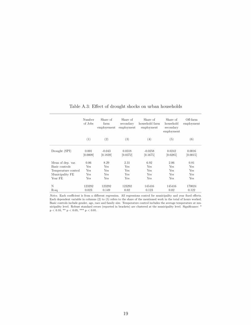
Table A.3: Effect of drought shocks on urban households



(1) (2) (3) (4) (5) (6)

Drought (SPI) 0.001 -0.043 0.0318 -0.0258 0.0242 0.0016[0.0009] [0.1839] [0.0372] [0.1675] [0.0285] [0.0015]


N 123292 123292 123292 145416 145416 170024R-sq 0.023 0.149 0.02 0.123 0.02 0.122

Notes. Each coefficient is from a different regression. All regressions control for municipality and year fixed effects.Each dependent variable in columns (2) to (5) refers to the share of the mentioned work in the total of hours worked.Basic controls include gender, age, race and family size. Temperature control includes the average temperature at mu-nicipality level. Robust standard errors (reported in brackets) are clustered at the municipality level. Significance: *p < 0.10, ** p < 0.05, *** p < 0.01.

19

Weather Shocks and Labor Allocation: Evidence from ... · Weather Shocks and Labor Allocation:...

Documents

Transcript of Weather Shocks and Labor Allocation: Evidence from ... · Weather Shocks and Labor Allocation:...