Weakly supervised graph based semantic segmentation by learning communities

of image-parts

Niloufar Pourian, S. Karthikeyan, and B.S. Manjunath

Department of Electrical and Computer Engineering, University of California, Santa Barbara, CA

npourian@ece.ucsb.edu, karthikeyan@ece.ucsb.edu, manj@ece.ucsb.edu

Abstract

We present a weakly-supervised approach to semantic

segmentation. The goal is to assign pixel-level labels given

only partial information, for example, image-level labels.

This is an important problem in many application scenar-

ios where it is difficult to get accurate segmentation or not

feasible to obtain detailed annotations. The proposed ap-

proach starts with an initial coarse segmentation, followed

by a spectral clustering approach that groups related image

parts into communities. A community-driven graph is then

constructed that captures spatial and feature relationships

between communities while a label graph captures corre-

lations between image labels. Finally, mapping the image

level labels to appropriate communities is formulated as a

convex optimization problem. The proposed approach does

not require location information for image level labels and

can be trained using partially labeled datasets. Compared

to the state-of-the-art weakly supervised approaches, we

achieve a significant performance improvement of 9% on

MSRC-21 dataset and 11% on LabelMe dataset, while be-

ing more than 300 times faster.

1. Introduction

We consider the problem of semantic segmentation to

predict a label for every image pixel. Semantic segmenta-

tion benefits a variety of vision applications, such as object

recognition, automatic driver assistance and 3D urban mod-

eling. However in practice, two key factors limit the ap-

plicability of semantic segmentation: speed and scalability.

In this work we develop an effective semantic segmentation

method which addresses these issues.

Semantic segmentation approaches can be broadly cat-

egorized into fully supervised, weakly supervised and un-

supervised methods. There is a wealth of published liter-

ature on fully supervised semantic segmentation that rely

on location information associated with image labels (fully

segmented training data) [3, 5, 7, 8, 9, 17, 18, 20, 23, 25,

26, 29, 31, 36, 40, 41, 42, 45, 49, 50, 55]. The aforemen-

tioned approaches require that every pixel in the training

set be manually labeled. The work in [8] considers a set-

ting in which the training dataset is a mixture of object seg-

ments and a set of objects’ bounding boxes. Despite adding

more flexibility, [8] still depends on the manual localiza-

tion of objects by a combination of regional segments and

bounding boxes. The approaches of [9, 55] focus on seg-

mentation templates to address the problem of image label-

ing. Such approaches have computational advantages over

pixel-based approaches by constraining the search process,

however, they still depend on providing the ground truth of

object boundaries in training. Creating annotations is costly

and time-consuming, thus limiting the applicability of the

aforementioned approaches to small sized datasets.

In order to scale semantic segmentation to larger

datasets, weakly supervised semantic segmentation ap-

proaches have been proposed [1, 30, 44, 46, 47, 48, 52, 53].

These methods typically require fully annotated image-level

labels without relying on location information associated to

image labels. These approaches use image-level object an-

notations to learn priors. Although more flexible than fully

supervised methods, these techniques typically assume that

one has access to all annotations associated with the image

which still limits their practical applicability. Our work is

closely related to the weakly supervised approaches while

being applicable to both fully/partially labeled datasets.

We note that there are segmentation methods that work

with unlabeled data, for example see [51], but they tend

to be not very robust given the under-constrained nature of

the problem. Label correlation enhance the performance by

providing stronger priors and unsupervised approaches are

inherently unable to do that.

Several works have utilized multiple segmentations to

address the problem of semantic segmentation by either

changing the parameters of a bottom-up approach [19, 24],

or by using different segmentation methods [10, 21, 34].

To avoid the increased complexity associated with multiple

segmentations, our model learns image parts using a single

segmentation by jointly considering the visual and spatial

11359

communities labels

L1

L3

Training

phase

(1) graph of segmented regions (2) learn communities (3) mapping labels to communities

(2) community image(1) segmented image labeled imageimage

Test

phase

L2

L1,L3

L2,L3

L2

L3

L1

L2

L3

Background

L2

L1, L3

L2, L3

Database

Figure 1: The overall framework of the proposed approach discussed in section 2. This includes the following steps in the reaining phase:

(1) graph of segmented regions, (2) community detection, and (3) mapping labels to the learned communities. The test phase consists of (1)

segmentation, and (2) mapping regions to the semantically learned communities. Li with i = 1, . . . , 3 indicates the image level labels

associated with training images. At test time, mapping regions of a given image to the learned commnunities results in a semantically

labeled image.

characteristics of all the images together. This ensures ro-

bustness to segmentation variations. In addition, many re-

searchers address the problem of semantic segmentation by

finding the labels associated with each pixel or superpixel

in the image [40, 48, 52].

In addition, there has been considerable interest in

object-based methods for semantic segmentation [2, 14, 27,

33, 43]. In particular, the work in [2, 14] focus on repre-

sentation and classification of individual regions by design-

ing region-based object detectors and subsequently com-

bining their outputs. This requires generating hierarchical

tree of regions at different levels of contrast, and dealing

with a large number (i.e. 1000) of generic regions per im-

age which is computationally expensive. Another research

area relevant to semantic segmentation is co-segmentation

[11, 38, 54]. Here, images which share semantic content

are segmented together to extract meaningful common in-

formation.

Additionally, several semantic segmentation approaches

involve solving a non-convex optimization problem [10, 24,

30, 48]. A solution to a non-convex formulation might only

be a local optima and there is no guarantee that the solution

is a global one. In particular, [30] involves solving an itera-

tive optimization which is computationally costly and does

not necessarily converge to an optimal solution. In contrast,

our formulation deals with a convex optimization problem

that can be solved efficiently [4].

Main Contributions: Based on image segmentation, we

use an attributed graph to capture the visual and spatial

characteristics of different image-parts. The communities

of related segmented regions among all images are discov-

ered by applying a spectral graph partitioning algorithm to

segregate highly related segments. This results in finding

meaningful image-part groupings. The relationships among

communities and labels are separately modeled. An opti-

mization framework is introduced as a graph learning ap-

proach to derive an appropriate semantic for each detected

object/community within an image. The overall framework

of the proposed approach is depicted in Figure 1. Summa-

rizing,

• Our formulation encodes label co-occurrences and in-

troduces a convex minimization problem for mapping

labels to communities. This optimization problem has

a closed form solution and can be efficiently solved.

• We learn groups of related image regions and then map

higher level semantics to small number of detected

communities, eliminating the need for pixel-wise se-

mantic mappings. This makes our method computa-

tionally efficient.

• The proposed work is robust to segmentation varia-

tions and does not require manual segmentation in

training or testing phases. In addition, this method can

be applied to databases where image-level labels are

only partially provided.

2. Approach

The proposed system learns different parts of an image

by grouping related image-parts and labeling each object

present in the image with its high level semantics. The de-

tails of our approach is as follows.

2.1. Image­Driven Graph

Inspired by [37, 48], we introduce an image-driven graph

to capture both visual and spatial characteristics of image

regions. This is followed by a graph partitioning algorithm

1360

1

13

2

15

3

8

4

14

10

16

5

117

6

9

C2

C1 C3

C4

12C5

Community-Driven Graph Label Graph

L1 L2

L3 L4

C2

C1 C3

C5

C4

Image-Driven Graph

Figure 2: Image-driven graph (top), community-driven graph (bot-

tom left), label graph (bottom right), along with the initial and fi-

nal label estimations for each of the detected communities. Each

node Ii in the fused data graph denotes a segmented region be-

longing to an image i from the database. Each node cj in the

community-driven graph denotes a detected community in the

fused data graph. Each node Lk in the label graph represents a

unique label. Each dotted ellipse represents a detected community

clustering related nodes (segmented regions) together. The solid

and dotted lines between the label graph and community-driven

graph represent the initial and final label assignemts to communi-

ties, respectively.

to segregate highly related regions across all images in the

database.

To provide spatial information, we utilize a segmenta-

tion algorithm based on color and texture [13]. We define

G(I) = (V (I), A(I)) to be the image-driven graph with

V (I) and A(I) representing the nodes and edges, respec-

tively. The image-driven graph G(I) containsD∑

d=1

|vd| num-

ber of nodes, where |vd| denotes the number of segmented

regions of image d, and D is the total number of images

in the database. Two nodes i and j are connected if they

are spatially adjacent or if they are visually similar. This is

summarized as the following:

A(I)ij = I(i ∈ Fj or i ∈ Hj), ∀i, j ∈ V (I) (1)

where I(x) is an indicator function and is equal to 1 if x

holds true and zero otherwise. In addition, Fj indicates the

set of all nodes (segmented regions) that are visually sim-

ilar to node j and Hj is the set of all nodes in the spatial

neighborhood of node j.

To represent each segmented region, DenseSift features

[32] are extracted from each image and then quantized into a

visual codebook. To form a regional signature hi for a node

i, features are mapped to the segmented regions that they

belong to and a histogram representation of the codebook is

constructed.

Two nodes i and j are considered visually similar if their

visual similarity score is higher than a threshold α > 0. The

visual similarity score is defined by the following:

Λ(hi, hj) = e−∆(hi,hj)︸ ︷︷ ︸

regional similarity

I(uTi uj > 0)

︸ ︷︷ ︸

label similarity

(2)

where ∆(hi, hj) represents the distance between the re-

gional representations of node i and j, and ui denotes a

binary label vector of node i with length equal to the to-

tal number of labels in the dataset. uij is equal to one iff

node i is associated with label j. Each node is associated

with the labels of the image that they belong to. Label sim-

ilarity limits us to consider visual similarity between nodes

that share label(s). The distance between two regional his-

tograms is measured by the Hellinger distance. This is a

suitable for computing the distance between histograms in

classification and retrieval problems [35].

2.2. Community­Driven Graph

Our goal is to find similar/related image-parts in the

graphical image representation. This is done by applying

a graph partitioning algorithm to the image-driven graph.

We refer to each of these groups as a community. Each

community resembles a bag of related image-parts.

For graph partitioning, we use the normalized cut

method as described in [39]. In this algorithm, the qual-

ity of the partition (cut) is measured by the density of

the weighted links inside communities as compared to the

weighted links between communities. The objective is to

maximize sum of the weighted links within a community

while minimizing sum of the weighted links across com-

munity pairs.

Suppose graph G(I) consists of C detected communities.

Each community ci with i = 1, . . . , C contains all the

pieces/image-parts of an object and by mapping these com-

munities to each segmented image, one can detect any spe-

cific object. Figure 3 illustrates some sample images high-

lighted by a color representing the community that each

segmented region belongs to. It is worth noting that if

we choose C to be small (fewer number of communities),

the detected communities may be such that they include all

parts of a particular object as a whole. While larger values

of C result in a case that different parts of objects fall into

different communities.

We define a community-driven data graph G(C) =(V (C), A(C)) where V (C), A(C) represent the nodes and

edges of this graph, respectively. Each node in graph G(C)

represents a detected community in graph G(I). A(C)ij repre-

1361

(a)

(b)

(c)

Figure 3: Row (a) illustrates four sample images from the VOC

2011 database. Row (b) represents the corresponding segmenta-

tions of the samples images. Each color denotes a segmented re-

gion. The segmentation is derived by the software provided by

[13]. In row (c), each color denotes a community that the seg-

mented regions of figures in row (b) belong to. These communi-

ties belong to the set of all detected communities over the entire

database. The community detection algorithm is described in Sec-

tion 2.2.

sents the number of links between the nodes of community

i and community j in graph G(I).

2.3. Label Graph

Let G(L) = (V (L), A(L)) represent a label graph with

V (L) and A(L) denoting the nodes and edges. Here, V (L)

is a set of all labels presented in the database and A(L)ij de-

notes the label correlation among two nodes i and j. Label

correlation is determined using a set of training instances

annotated for the label set. A binary vector vi of length

equal to the number of training instances is created for each

label i. vi(j) is equal to one iff the jth training instance

is annotated with the ith label. We use the standard cosine

similarity to specify the correlation between the labels.

Since the database images may only be partially labeled

by a subset of objects, we add an extra label called “back-

ground” for regions with no label associated to them in the

database.

2.4. Initialization of Community Labels

In the fully labeled dataset where the background class is

absent, each segmented region is initially associated with all

of its image-level labels. We define initial labeling for each

of the detected communities by matrix Y = (Y1, . . . , YC)′

of dimension C × K with C being equal to the total number

of detected communities and K denoting the total number

of labels in the dataset. Yij represents the number of nodes

in community ci that are associated with label j. Multiple

nodes from the same image in community ci are counted as

one. Each row vector Yi, i = 1, . . . , C, is ℓ1 normalized

to give comparable label association to each of the com-

munities independent of the number of nodes they contain.

Next, we binarize each vector Yi using a threshold β as:

Yij = I(Yij > β). (3)

For partially labeled datasets, we consider to have an addi-

tional column for Y corresponding to the background label.

If Yij = 0, ∀j ∈ 1, . . . ,K, we set Yi(K+1) = 1 to asso-

ciate that community with a “background” label. This is to

compensate for partially labeled datasets. In the remainder

of this paper, for partially labeled datasets, we assume Kdenotes the total number of labels in the dataset as well as

the “background” label.

Algorithm 1 Mapping semantics to detected communities

Input: G(I), A(L), A(C), C,K, β, ci ∀i ∈ 1, . . . , COutput: U

Rij : set of nodes in community ci & image-level label j

Comment: Initialization of detected communities

Y ← C ×K zero vector

for i = 1→ C do

for j = 1→ K do

if |Rij | ≥ β then

Y (i, j)← 1end if

end for

end for

Comment: Associate each community with a label

Solve Equation (9) for X

for i = 1→ C do

Uci ← max(X(i, :))end for

2.5. Mapping Labels to Communities

We assume that every image segment represents a spe-

cific image label. By extending this idea, we want to asso-

ciate each community with the most appropriate semantic

label. In this section, we describe how each community is

associated with a semantic label as shown in Figure 4. Let

A(C) be an C × C affinity matrix of the community-driven

graph with C = |V (C)|. Let A(L) be a K × K affinity ma-

trix denoting the label graph constructed for the K concepts

(labels). Let X = (X1, . . . , XC)′ = (E1, . . . , EK) be a

C ×K matrix defining the final labeling associated to every

community derived in the previous section. Similarly, let

Y = (Y1, . . . , YC)′ be a C × K matrix denoting the initial

label assignments to every community.

To assign a label to each community, we construct an

optimization problem with the following properties:

(a) highly correlated labels to be assigned to highly

correlated communities

(b) weakly connected communities have distinct labels

(c) small label deviation from initial label for each

community.

Given a set of communities C = c1, c2, . . . , cC, and their

affinity matrix A(C), the objective function to classify each

1362

community with a unique label L = l1, l2, ..., lK is de-

fined as follows:

Ω(X) =1

2

K∑

i,j=1

A(L)ij

∥∥∥∥∥∥

Ei√

D(L)ii

−Ej

√

D(L)jj

∥∥∥∥∥∥

2

︸ ︷︷ ︸

(a)

+

λ

C∑

i,j

A(C)ij ‖Xi −Xj‖

2

︸ ︷︷ ︸

(b)

+µ

C∑

i

‖Xi − Yi‖2

︸ ︷︷ ︸

(c)

.

(4)

where D(L) is a diagonal matrix whose (i, i) entries are

equal to the sum of the i-th row of A(L), i.e. D(L)ii =

∑Kj=1 A

(L)ij . Next, the solution X that minimizes (4) is de-

rived.

The first term on the right hand side of Equation (4) can

be written as:

12

K∑

i,j=1

A(L)ij

∥∥∥∥∥∥

Ei√

D(L)ii

−Ej

√

D(L)jj

∥∥∥∥∥∥

2

= 12

K∑

i=1

ETi Ei +

K∑

j=1

ETj Ej − 2

K∑

i,j=1

A(L)ij

ETi Ei

√

D(L)i

D(L)j

=K∑

i=1

ETi Ei −

K∑

i,j=1

A(L)ij

ETi Ei

√

D(L)i

D(L)j

= tr(

ET(

I −D(L)(−1/2)A(L)D(L)(−1/2)

)

E)

= tr(XL1X

T),

(5)

with L1 = D(L)−D(L)(−1/2)A(L)D(L)(−1/2)

. The second

term in (4) can be written as:

C∑

i,j

A(C)ij ‖Xi −Xj‖

2

=C∑

i

C∑

j

A(C)ij (Xi −Xj)

T (Xi −Xj)

=C∑

i

C∑

j

A(C)ij

(XT

i Xi +XTj Xj − 2XT

j Xi

)

= 2∑

i

XiXTi

(

A(C)ij

)

− 2∑

i

∑

j

A(C)ij XT

i Xi

= tr(

XTD(C)X)

− tr(

XTA(C)X)

= tr(

XT (D(C) −A(C))X)

= tr(XT

L2X),

(6)

with L2 = D(C) −A(C). Thus, the cost function in (4) can

be summarized as:

Ω(X) = tr(XL1X

T)+ λtr

(XT

L2X)+ µ‖X − Y ‖2.

(7)

Ω(X) in (7) is a convex function of X . By taking the deriva-

tive of (7) with respect to X , we get:

d(Ω(X))dX = 0→ 2XL1 + 2λL2X + 2µ(X − Y ) = 0,

(8)

Community Mapped Image Semantic Labels

label 1

label 2

label 3

label 4

Segmented Image

Figure 4: Illustration of mapping the communities to semantic la-

bels. The colored circles on the right are denoting the semnatic

labels across the dataset. Image is best viewed in color.

which can be written as:

(µI + λL2)X +XL1 = µY. (9)

Equation (9) is a Lyapunov equation of the form AQ +QB = C. The solution to (9) can be obtained using ex-

isting software libraries.

Once X is found, we use the following formulation to

assign a single label to each community ci:

Uci = argmaxj Xij , ∀j ∈ 1, ...,K . (10)

To maximize the performance, one can apply a line-search

by stepping through the threshold β (threshold used to bina-

rize the initial label matrix Y ), and choose the one that re-

sults in the highest performance. This process is illustrated

in Algorithm 1.

It is worth noting that instead of choosing the label with

maximum likelihood for each community, one could add an

additional constraint by defining each Xi as a binary vec-

tor and enforcing unit ℓ1 norm of Xi (minimizing ‖Xi‖1).

However, we did not follow such a formulation as it would

require solving an integer programming problem which re-

sults in a non-convex optimization.

Figure 2 illustrates the image-driven graph, community-

driven graph, label graph, along with the initial and final

label estimations for each of the detected communities.

2.6. Generalizing to a Test Image

First, we segment each test image Q. To determine

the association between each of its segmented regions and

the detected communities, we follow [37] and provide a

brief summary. Let Hi denote the set of all nodes in the

spatial neighborhood of node i, cj be a community with

j ∈ 1, . . . , C, and T ′i denote the set of all nodes that are

in the top T ′ nearest neighbors of node i. The strength of as-

sociation of a node i to a community cj is measured by two

factors: first by the attribute similarity between node i and

community cj , second by considering the attribute similar-

ity between neighbors of node i and different communities

in the network along with the relation between community

cj and each of the communities in the network.

1363

Let g(i ∈ cj) denote the attribute similarity between

node i and community cj . The function g(i ∈ cj) is de-

fined by the fraction of top T ′ nearest neighbors to node i

that belong to community cj :

g(i ∈ cj) =

∑

k∈T ′k

Ik∈cj

T ′ .(11)

Moreover, f(cj′ , cj) is defined to measure the relation be-

tween two communities cj′ and cj :

f(cj′ , cj) =

∑

i∈cj′

∑

k∈cj

I

A(I)ik

>0

∑

i∈cj′

|V (I)|∑

k=1

I

A(I)ik

>0

(12)

where |V (I)| denotes the total number of nodes in the

image-driven graph. In particular, f(cj′ , cj) measures the

number of links between the two communities cj′ and cjdivided by the total number of links between community

cj′ and all other communities. Thus, the strength of associ-

ation of a node i to a community cj can be determined by

π(i)j :

π(i)j =

∑

k∈Hi

[

C∑

j′=1

f(cj′ ,cj)g(k∈cj′ )

]

g(i∈cj)

C∑

j′′=1

∑

k∈Hi

[

C∑

j′=1

f(cj′′ ,cj′ )g(k∈cj′ )

]

g(i∈cj′′ )

, (13)

where C denotes the total number of detected communities.

Finally, each segmented region i is mapped to community c

with the highest association:

c = argmaxj

π(i)j , (14)

and is semantically labeled accordingly.

3. Experimental Results

To demonstrate the applicability of the proposed method,

four commonly used datasets for semantic segmentation

are considered: MSRC-21 [12], LabelMe [28], VOC 2009

[15] and VOC 2011 [16]. Our approach does not require

groundtruth segmentation in the training phase.

To measure the performance, we choose the common av-

erage per-class accuracy which measures the percentage of

correctly classified pixels for a class and then averages over

all classes. This measurement avoids bias towards classes

that occupy larger image areas, such as sky or grass. It also

penalizes a model that maximizes agreement simply by pre-

dicting very few labels overall.

We investigate how the performance of our method

varies as the level of segmentation changes. We further

evaluate the performance of our system as a function of the

number of detected communities C. In addition, the sensi-

tivity of our approach on parameter β, the threshold used to

binarize initial label vectors, is illustrated. Furthermore, the

performance of this work is compared against the state of

the art weakly supervised semantic segmentation methods

as well as fully supervised methods. Finally, the computa-

tional cost of the proposed approach is discussed.

3.1. Database

In our experiments, we use MSRC-21, LabelMe, and

VOC 2009 and VOC 2011 datasets. We do not use any

location information associated with the label annotations

in training or testing phase for any of these datasets. At

training phase, only the image-level labels are considered.

MSRC-21: This is a publicly available dataset contain-

ing 591 images. This dataset is a fully annotated dataset

with 21 object classes. To make a fair comparison, we eval-

uate the performance of our system on MSRC-21 as the ma-

jority of the weakly supervised approaches are also evalu-

ated on this dataset. Ground-truth semantic segmentation

information of MSRC-21 is only used to measure the accu-

racy of the proposed system.

LabelMe: This is a more challenging dataset than

MSRC-21. It includes 2, 688 images from 33 classes and is

fully annotated. Similar to MSRC-21 dataset, the ground-

truth semantic segmentation information is only used to

measure the accuracy of our system.

VOC 2009, 2011: This dataset is a publicly available

dataset with partial labeling. There are 20 labeled objects

and 1 background class. We choose to evaluate the per-

formance on VOC as each image contains multiple classes

while being only partially labeled. This is a more challeng-

ing dataset as a single background class covers several ob-

ject classes such as “sky” and “grass”. It addition, there are

more significant background clutter, illumination changes

and occlusions.

3.2. Evaluation

Performance: In Figure 5, we demonstrate the perfor-

mance when the segmentation level varies. By setting the

parameters of [13], we achieve three levels of segmentation

with an average number of 20, 50, and 70 segments per im-

age which are referred to as “Coarse”, “Mid”, and “Fine”,

respectively. It can be seen that “Fine” segmentation level

has the highest performance accuracy. This can be predicted

as at “Fine” level more spatial information is encoded which

provides different objects with more accurate outlines and

thus higher performance. Furthermore, Figure 5 illustrates

the effect of the number of detected communities on the per-

formance accuracy. For MSRC-21 dataset, the performance

of the proposed approach remains nearly invariant when the

number of detected communities is larger than 500.

Figure 6 illustrates the performance as a function of

threshold β. As expected, extremely large or small val-

ues of β can degrade the performance. This effect can be

justified as large values result in removing the majority of

1364

1 501 1001 15010.87

0.88

0.89

0.9

0.91

Number of Communities (C)

Accuracy

Fine Segmentation levelMid Segmentation levelCoarse Segmentation level

Figure 5: Effect of different levels of segmentation as well as dif-

ferent number of detected communities on the performance accu-

racy. Results are reported for MSRC-21 dataset.

0 0.1 0.2 0.3 0.4 0.5 0.6 0.70.7

0.75

0.8

0.85

0.9

Threshold

Accuracy

Figure 6: Performance of the proposed appraoch against threshold

β. Results are reported for MSRC-21 dataset.

initial community labelings while small β results in having

a large group of initial labelings per image. We notice that

our method is robust to selection of the parameter β as well.

The per-class performance accuracy between the pro-

posed approach and the baseline methods [44], [48], and

[53] is compared in Table 1. Our approach achieves a

higher average per-class accuracy than the baseline meth-

ods. We have also included the state of the art results of

fully-supervised methods [7], [3], [36], and [50] reported on

MSRC-21 dataset. Our approach is even comparable with

the fully-supervised ones without requiring ground-truth la-

beling at training time.

Furthermore, Table 2 demonstrate that the average per-

class accuracy of the proposed work on LabelMe dataset

compares competitively with the state of the art results. The

approach of [31] achieves an average accuracy of 51.7%while being fully supervised (requires ground truth segmen-

tation in the training phase) and involves training a convo-

lutional neural network (CNN). Again, we note that our ap-

proach does not require complete supervision. In general,

the learning capacity of these networks depends on the num-

ber and size of the kernels in each layer and the number of

kernel combinations between layers. The work of [31] has

roughly more than a million parameters which leads to the

training time of more than three days on a GPU. A detailed

analysis of computational complexity of our approach shall

be discussed shortly.

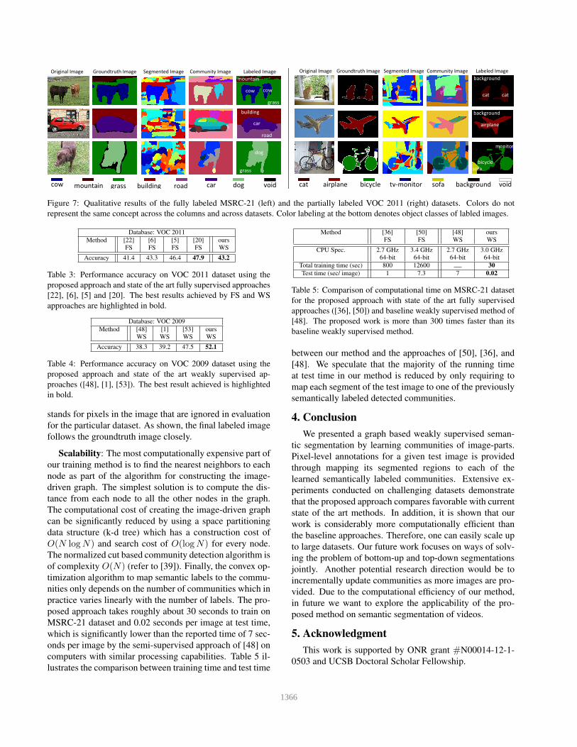
Database: MSRC-21

Method [7] [3] [36] [50] [44] [48] [53] ours

FS FS FS FS WS WS WS WS

building 66 70 71 45 12 89

grass 87 98 98 64 83 97

tree 84 87 90 71 70 89

cow 81 76 79 75 81 94

sheep 83 79 86 74 93 92

sky 93 96 93 86 84 96

airplane 81 81 88 81 91 89

water 82 75 86 47 55 87

face 78 86 90 1 97 88

car 86 74 84 73 87 96

bicycle 94 88 94 55 92 89

flower 96 96 98 88 82 87

sign 87 72 76 6 69 90

bird 48 36 53 6 51 82

book 90 90 97 63 61 89

chair 81 79 71 18 59 79

road 82 87 89 80 66 77

cat 82 74 83 27 53 87

dog 75 60 55 26 44 89

body 70 54 68 55 9 88

boat 52 35 17 8 58 96

average 94.5 80 76 79.3 50 67 80 89

Table 1: Per-class accuracy on MSRC-21 using the proposed ap-

proach, state of the art fully supervised approaches ( [7], [3], [36],

[50] ) and weakly supervised methods ([44], [48], [53]). FS and

WS denote fully-supervised and weakly-supervised approaches.

The best results achieved by FS and WS approaches are high-

lighted in bold. Our method achieves 9% improvement compared

to WS approaches, while being comparable to FS approaches.

Database: LabelMe

Method [41] [43] [31] [44] [30] [53] ours

FS FS FS WS WS WS WS

Accuracy 13 41 51.7 14 25 33.37 44

Table 2: Performance accuracy on LabelMe dataset using the pro-

posed approach, state of the art fully supervised approaches ([41],

[43], [31]) and weakly supervised methods ([44], [30], [53]). The

best results achieved by FS and WS approaches are highlighted in

bold. We achieve 11% improvement compared to WS approaches,

while being comparable to FS approaches.

By applying the proposed approach to partially labeled

VOC 2011 dataset, we achieve an average accuracy of

43.2%. To the best of our knowledge, no weakly super-

vised results were reported on this dataset yet. Table 3 re-

ports the results achieved by our approach and the state of

the art fully-supervised methods. It can be seen that our

approach is achieving comparable performance while be-

ing only weakly supervised. It is worth noting that [20]

achieves its performance using a pre-trained CNN on a large

auxiliary dataset and then fine-tuned for VOC 2011. Also,

[5] uses additional external ground truth segmentations.

Table 4 illustrates that the proposed approach achieves

higher performance accuracy than the state of the art weakly

supervised approaches which are trained and tested on VOC

2009 dataset.

In addition, Figure 7 illustrates step-by-step qualitative

results on the fully labeled MSRC-21 dataset and the par-

tially labeled VOC 2011 dataset. In this Figure, label “void”

1365

Original Image Segmented Image Community Image Labeled Image

cow

grass

cow

mountain

grassmountain road car

Groundtruth Image

car

road

building

dogbuildingcow

dog

grass

void

Original Image Segmented Image Community Image Labeled Image

airplane

Groundtruth Image

bicyclecat background

cat cat

background

background

airplane

voidtv-monitor sofa

bicycle

sofa

monitor

Figure 7: Qualitative results of the fully labeled MSRC-21 (left) and the partially labeled VOC 2011 (right) datasets. Colors do not

represent the same concept across the columns and across datasets. Color labeling at the bottom denotes object classes of labled images.

Database: VOC 2011

Method [22] [6] [5] [20] ours

FS FS FS FS WS

Accuracy 41.4 43.3 46.4 47.9 43.2

Table 3: Performance accuracy on VOC 2011 dataset using the

proposed approach and state of the art fully supervised approaches

[22], [6], [5] and [20]. The best results achieved by FS and WS

approaches are highlighted in bold.

Database: VOC 2009

Method [48] [1] [53] ours

WS WS WS WS

Accuracy 38.3 39.2 47.5 52.1

Table 4: Performance accuracy on VOC 2009 dataset using the

proposed approach and state of the art weakly supervised ap-

proaches ([48], [1], [53]). The best result achieved is highlighted

in bold.

stands for pixels in the image that are ignored in evaluation

for the particular dataset. As shown, the final labeled image

follows the groundtruth image closely.

Scalability: The most computationally expensive part of

our training method is to find the nearest neighbors to each

node as part of the algorithm for constructing the image-

driven graph. The simplest solution is to compute the dis-

tance from each node to all the other nodes in the graph.

The computational cost of creating the image-driven graph

can be significantly reduced by using a space partitioning

data structure (k-d tree) which has a construction cost of

O(N logN) and search cost of O(logN) for every node.

The normalized cut based community detection algorithm is

of complexity O(N) (refer to [39]). Finally, the convex op-

timization algorithm to map semantic labels to the commu-

nities only depends on the number of communities which in

practice varies linearly with the number of labels. The pro-

posed approach takes roughly about 30 seconds to train on

MSRC-21 dataset and 0.02 seconds per image at test time,

which is significantly lower than the reported time of 7 sec-

onds per image by the semi-supervised approach of [48] on

computers with similar processing capabilities. Table 5 il-

lustrates the comparison between training time and test time

Method [36] [50] [48] ours

FS FS WS WS

CPU Spec. 2.7 GHz 3.4 GHz 2.7 GHz 3.0 GHz

64-bit 64-bit 64-bit 64-bit

Total training time (sec) 800 12600 30

Test time (sec/ image) 1 7.3 7 0.02

Table 5: Comparison of computational time on MSRC-21 dataset

for the proposed approach with state of the art fully supervised

approaches ([36], [50]) and baseline weakly supervised method of

[48]. The proposed work is more than 300 times faster than its

baseline weakly supervised method.

between our method and the approaches of [50], [36], and

[48]. We speculate that the majority of the running time

at test time in our method is reduced by only requiring to

map each segment of the test image to one of the previously

semantically labeled detected communities.

4. Conclusion

We presented a graph based weakly supervised seman-

tic segmentation by learning communities of image-parts.

Pixel-level annotations for a given test image is provided

through mapping its segmented regions to each of the

learned semantically labeled communities. Extensive ex-

periments conducted on challenging datasets demonstrate

that the proposed approach compares favorable with current

state of the art methods. In addition, it is shown that our

work is considerably more computationally efficient than

the baseline approaches. Therefore, one can easily scale up

to large datasets. Our future work focuses on ways of solv-

ing the problem of bottom-up and top-down segmentations

jointly. Another potential research direction would be to

incrementally update communities as more images are pro-

vided. Due to the computational efficiency of our method,

in future we want to explore the applicability of the pro-

posed method on semantic segmentation of videos.

5. Acknowledgment

This work is supported by ONR grant #N00014-12-1-

0503 and UCSB Doctoral Scholar Fellowship.

1366

References

[1] A. Vezhnevets, V. Ferrari, and J. M. Buhmann. Weakly supervised

structured output learning for semantic segmentation. In CVPR,

2012.

[2] P. Arbelaez, B. Hariharan, C. Gu, S. Gupta, L. Bourdev, and J. Malik.

Semantic segmentation using regions and parts. In CVPR, 2012.

[3] X. Boix, J. M. Gonfaus, J. van de Weijer, A. D. Bagdanov, J. Serrat,

and J. Gonzalez. Harmony potentials. IJCV, 2012.

[4] S. Boyd and L. Vandenberghe. Convex optimization. Cambridge

university press, 2009.

[5] J. Carreira, R. Caseiro, J. Batista, and C. Sminchisescu. Semantic

segmentation with second-order pooling. In ECCV. 2012.

[6] J. Carreira, F. Li, and C. Sminchisescu. Object recognition by se-

quential figure-ground ranking. IJCV, 2012.

[7] J. Carreira and C. Sminchisescu. Cpmc: Automatic object segmen-

tation using constrained parametric min-cuts. PAMI, 2012.

[8] F.-J. Chang, Y.-Y. Lin, and K.-J. Hsu. Multiple structured-instance

learning for semantic segmentation with uncertain training data. In

CVPR, 2014.

[9] L.-C. Chen, G. Papandreou, and A. L. Yuille. Learning a dictionary

of shape epitomes with applications to image labeling. In ICCV,

2013.

[10] X. Chen, A. Jain, A. Gupta, and L. S. Davis. Piecing together the

segmentation jigsaw using context. In CVPR, 2011.

[11] X. Chen, A. Shrivastava, and A. Gupta. Enriching visual knowledge

bases via object discovery and segmentation. In CVPR, 2014.

[12] A. Criminisi, T. Minka, and J. Winn. Microsoft re-

search cambridge object recognition image dataset. version

2.0, 2004. Available at http://research.microsoft.com/en-

us/projects/objectclassrecognition/.

[13] Y. Deng and B. Manjunath. Unsupervised segmentation of color-

texture regions in images and video. PAMI, 2001.

[14] J. Dong, Q. Chen, S. Yan, and A. Yuille. Towards unified object

detection and semantic segmentation. In ECCV. 2014.

[15] M. Everingham, L. Van Gool, C. Williams, J. Winn, and A. Zisser-

man. The pascal visual object classes challenge 2009. In 2th PASCAL

Challenge Workshop, 2009.

[16] M. Everingham, L. Van Gool, C. K. Williams, J. Winn, and A. Zisser-

man. The pascal visual object classes (voc) challenge. IJCV, 2010.

[17] C. Farabet, C. Couprie, L. Najman, and Y. LeCun. Learning hierar-

chical features for scene labeling. PAMI, 2013.

[18] B. Fulkerson, A. Vedaldi, and S. Soatto. Class segmentation and

object localization with superpixel neighborhoods. In CVPR, 2009.

[19] C. Galleguillos, B. Babenko, A. Rabinovich, and S. Belongie.

Weakly supervised object localization with stable segmentations. In

ECCV, 2008.

[20] R. Girshick, J. Donahue, T. Darrell, and J. Malik. Rich feature hier-

archies for accurate object detection and semantic segmentation. In

CVPR, 2014.

[21] A. Gupta, A. A. Efros, and M. Hebert. Blocks world revisited: Image

understanding using qualitative geometry and mechanics. In ECCV,

2010.

[22] A. Ion, J. Carreira, and C. Sminchisescu. Probabilistic joint image

segmentation and labeling. In Advances in Neural Information Pro-

cessing Systems, 2011.

[23] P. Kohli, P. H. Torr, et al. Robust higher order potentials for enforcing

label consistency. IJCV, 2009.

[24] M. P. Kumar and D. Koller. Efficiently selecting regions for scene

understanding. In CVPR, 2010.

[25] L. Ladicky, C. Russell, P. Kohli, and P. H. Torr. Associative hierar-

chical crfs for object class image segmentation. In CVPR, 2009.

[26] L. Ladicky, C. Russell, P. Kohli, and P. H. Torr. Graph cut based

inference with co-occurrence statistics. In ECCV, 2010.

[27] C. Li, D. Parikh, and T. Chen. Automatic discovery of groups of

objects for scene understanding. In CVPR, 2012.

[28] C. Liu, J. Yuen, and A. Torralba. Nonparametric scene parsing: Label

transfer via dense scene alignment. In CVPR, 2009.

[29] C. Liu, J. Yuen, and A. Torralba. Nonparametric scene parsing via

label transfer. PAMI, 2011.

[30] Y. Liu, J. Liu, Z. Li, J. Tang, and H. Lu. Weakly-supervised dual

clustering for image semantic segmentation. In CVPR, 2013.

[31] J. Long, E. Shelhamer, and T. Darrell. Fully convolutional networks

for semantic segmentation. arXiv preprint arXiv:1411.4038, 2014.

[32] D. Lowe. Object recognition from local scale-invariant features. In

ICCV, 1999.

[33] T. Malisiewicz and A. Efros. Beyond categories: The visual memex

model for reasoning about object relationships. In NIPS, 2009.

[34] T. Malisiewicz and A. A. Efros. Recognition by association via learn-

ing per-exemplar distances. In CVPR, 2008.

[35] M. S. NIKULIN. Hellinger Distance. Springer, 2001.

[36] D. Pei, Z. Li, R. Ji, and F. Sun. Efficient semantic image segmen-

tation with multi-class ranking prior. Computer Vision and Image

Understanding, 2014.

[37] N. Pourian and B. Manjunath. Pixnet: A localized feature repre-

sentation for classification and visual search. Trans. on Multimedia,

2015.

[38] M. Rubinstein, A. Joulin, J. Kopf, and C. Liu. Unsupervised joint ob-

ject discovery and segmentation in internet images. In CVPR, 2013.

[39] J. Shi and J. Malik. Normalized cuts and image segmentation. PAMI,

2000.

[40] J. Shotton, M. Johnson, and R. Cipolla. Semantic texton forests for

image categorization and segmentation. In CVPR, 2008.

[41] J. Shotton, J. Winn, C. Rother, and A. Criminisi. Textonboost: Joint

appearance, shape and context modeling for multi-class object recog-

nition and segmentation. In ECCV, 2006.

[42] J. Tighe and S. Lazebnik. Superparsing: scalable nonparametric im-

age parsing with superpixels. In ECCV, 2010.

[43] J. Tighe and S. Lazebnik. Finding things: Image parsing with regions

and per-exemplar detectors. In CVPR, 2013.

[44] J. Verbeek and B. Triggs. Region classification with markov field

aspect models. In CVPR, 2007.

[45] J. Verbeek and W. Triggs. Scene segmentation with crfs learned from

partially labeled images. In NIPS, 2008.

[46] A. Vezhnevets and J. M. Buhmann. Towards weakly supervised se-

mantic segmentation by means of multiple instance and multitask

learning. In CVPR, 2010.

[47] A. Vezhnevets, J. M. Buhmann, and V. Ferrari. Active learning for

semantic segmentation with expected change. In CVPR, 2012.

[48] A. Vezhnevets, V. Ferrari, and J. M. Buhmann. Weakly supervised

semantic segmentation with a multi-image model. In ICCV, 2011.

[49] L. Yang, P. Meer, and D. J. Foran. Multiple class segmentation using

a unified framework over mean-shift patches. In CVPR, 2007.

[50] J. Yao, S. Fidler, and R. Urtasun. Describing the scene as a whole:

Joint object detection, scene classification and semantic segmenta-

tion. In CVPR, 2012.

[51] H. Zhang, J. E. Fritts, and S. A. Goldman. Image segmentation eval-

uation: A survey of unsupervised methods. Computer Vision and

Image Understanding, 2008.

[52] L. Zhang, M. Song, Z. Liu, X. Liu, J. Bu, and C. Chen. Probabilistic

graphlet cut: Exploiting spatial structure cue for weakly supervised

image segmentation. In CVPR, 2013.

[53] L. Zhang, Y. Yang, Y. Gao, Y. Yu, C. Wang, and X. Li. A probabilistic

associative model for segmenting weakly-supervised images. Trans.

Image Processing, 2014.

[54] T. Zhou, Y. Jae Lee, S. X. Yu, and A. A. Efros. Flowweb: Joint image

set alignment by weaving consistent, pixel-wise correspondences. In

CVPR, 2015.

[55] L. Zhu, Y. Chen, Y. Lin, C. Lin, and A. Yuille. Recursive segmenta-

tion and recognition templates for image parsing. PAMI, 2012.

1367