Weak Lensing Tomography

Wayne HuFermilab, October 2002

z0.5 1 1.5 2

windows

1.4

1.2

1.0

0.8

0.6

0.60.40.2

mtot=0.2eV

Collaborators

• Chuck Keeton• Takemi Okamoto• Max Tegmark• Martin White

Collaborators

• Chuck Keeton• Takemi Okamoto• Max Tegmark• Martin White

Microsoft

http://background.uchicago.edu/~whu/Presentations/ferminu.pdf

Massive Neutrinos• Relativisticstressesof a light neutrinoslow thegrowthof structure

• Neutrino species withcosmological abundancecontribute to matterasΩνh

2 = mν/94eV, suppressing power as∆P/P ≈ −8Ων/Ωm

∆P

P≈ −0.6

(mtot

eV

)

Massive NeutrinosCurrent data from 2dF galaxy survey indicates mν<1.8eVassuming a ΛCDM model with parameters constrained by theCMB.

•

k (h Mpc-1)

P(k)

(h-

1 M

pc)3

0.1 10.01

103

104

105

2dF

Lensing Observables• Image distortiondescribed byJacobian matrixof the remapping

A =

1− κ− γ1 −γ2

−γ2 1− κ+ γ1

,

whereκ is theconvergence, γ1, γ2 are theshearcomponents

Lensing Observables• Image distortiondescribed byJacobian matrixof the remapping

A =

1− κ− γ1 −γ2

−γ2 1− κ+ γ1

,

whereκ is theconvergence, γ1, γ2 are theshearcomponents

• related to thegravitational potentialΦ by spatial derivatives

ψij(zs) = 2∫ zs

0dzdD

dz

D(Ds −D)

Ds

Φ,ij ,

ψij = δij − Aij, i.e. viaPoisson equation

κ(zs) =3

2H2

0Ωm

∫ zs

0dz

dD

dz

D(Ds −D)

Ds

δ/a ,

Gravitational Lensing by LSS

• Shearing of galaxy images reliably detected in clusters

• Main systematic effects are instrumental rather than astrophysical

Colley, Turner, & Tyson (1996)

Cluster (Strong) Lensing: 0024+1654

Cosmic Shear Data• Shear variance as a function of smoothing scale

compilation from Bacon et al (2002)

Shear Power Modes

• Alignment of shear and wavevector defines modes

ε

β

Shear Power Spectrum

• Lensing weighted Limber projection of density power spectrum

• ε−shear power = κ power

10 100 1000l

10–4

10–5

10–7

10–6

l(l+

1)C

l /2

πεε

k=0.02 h/Mpc

Limber approximation

Linear

Non-linear

Kaiser (1992)Jain & Seljak (1997)

Hu (2000)

zs=1

zs

PM Simulations

• Simulating mass distribution is a routine exercise

6∞ × 6∞ FOV; 2' Res.; 245–75 h–1Mpc box; 480–145 h–1kpc mesh; 2–70 109 M

Convergence Shear

White & Hu (1999)

Degeneracies• All parameters of initial condition, growth and distance redshift relation D(z) enter• Nearly featureless power spectrum results in degeneracies

10 100 1000l

10–4

10–5

10–7

10–6l(l+1

)Cl

/2

πεε

zs=1

Degeneracies• All parameters of initial condition, growth and distance redshift relation D(z) enter• Nearly featureless power spectrum results in degeneracies

• Combine with information from the CMB: complementarity (Hu & Tegmark 1999)

• Crude tomography with source divisions (Hu 1999; Hu 2001)

• Fine tomography with source redshifts (Hu & Keeton 2002; Hu 2002)

10 100

20

40

60

80

100

l (multipole)

∆T

CMB

MAPPlanck

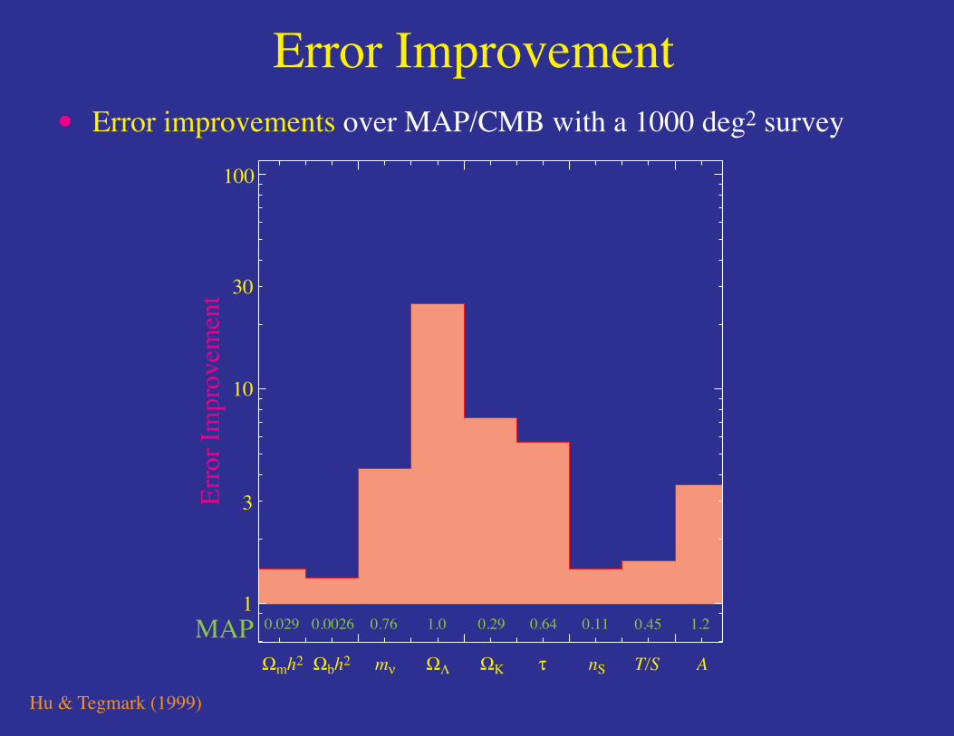
Error Improvement• Error improvements over MAP/CMB with a 1000 deg2 survey

Hu & Tegmark (1999)

0.029 0.0026 0.76 1.0 0.29 0.64 0.11 0.45 1.2

Ωmh2 Ωbh2 mν nS T/S AΩΛ ΩK τ

MAP

Erro

r Im

prov

emen

t

1

3

10

30

100

Crude Tomography

• Divide sample by photometric redshifts

Hu (1999)

1 2

2

D0 0.5

0.1

1

2

3

0.2

0.3

1 1.5 2.0

g i(D

) n i

(D)

(a) Galaxy Distribution

(b) Lensing Efficiency

22

100 1000 104

10–5

10–4

l

Pow

er

25 deg2, zmed=1

Crude Tomography

• Divide sample by photometric redshifts

• Cross correlate samples

• Order of magnitude increase in precision even after CMB breaks degeneracies

Hu (1999)

1

1

2

2

D0 0.5

0.1

1

2

3

0.2

0.3

1 1.5 2.0

g i(D

) n

i(D

)

(a) Galaxy Distribution

(b) Lensing Efficiency

22

11

12

100 1000 104

10–5

10–4

l

Pow

er

25 deg2, zmed=1

Efficacy of Crude Tomography• Error improvements over MAP/CMB with a 1000 deg2 survey

Hu & Tegmark (1999); Hu (2000)

0.029 0.0026 0.76 1.0 0.29 0.64 0.11 0.45 1.2

Ωmh2 Ωbh2 mν nS T/S AΩΛ ΩK τ

MAP

MAP +Er

ror I

mpr

ovem

ent

1

3

10

30

100

photo-zno-z

Dark Energy & Tomography

• Both CMB and tomography help lensing provide interesting constraints on dark energy

0 0.5 1.0

0

1

2

ΩDE

w

l<3000; 56 gal/deg2

MAPno–z

1000deg2

Hu (2001)

Dark Energy & Tomography

• Both CMB and tomography help lensing provide interesting constraints on dark energy

0 0.5 1.0

0

1

2

ΩDE

w

l<3000; 56 gal/deg2

MAPno–z3–z

1000deg2

Hu (2001)

Dark Energy & Tomography

• Both CMB and tomography help lensing provide interesting constraints on dark energy

0 0.5 1.0

0.55–1

–0.9

–0.8

–0.7

–0.6

0.6 0.65 0.7

0

1

2

ΩDE

w

l<3000; 56 gal/deg2

MAPno–z3–z

1000deg2

Hu (2001)

Dark Sector and Radial Information• Much of the information on the dark sector is hidden in the

temporalor radialdimension

• Evolution ofgrowth rate(dark energy pressure slows growth)

• Evolution ofdistance-redshiftrelation

• Lensing is inherentlytwo dimensional: all mass along the line ofsight lenses

• Tomography implicitly or explicitlyreconstructs radial dimensionwith source redshifts

• Photometric redshift errors currently∆z < 0.1 out toz ~ 1 andallow for ”fine” tomography

Fine Tomography• Convergence– projection of∆ = δ/a for eachzs

κ(zs) =3

2H2

0Ωm

∫ zs

0

dzdD

dz

D(Ds −D)

Ds

∆ ,

Fine Tomography• Convergence– projection of∆ = δ/a for eachzs

κ(zs) =3

2H2

0Ωm

∫ zs

0

dzdD

dz

D(Ds −D)

Ds

∆ ,

• Data islinear combinationof signal + noise

dκ = Pκ∆s∆ + nκ ,

[Pκ∆]ij =

32H2

0ΩmδDj(Di+1−Dj)Dj

Di+1Di+1 > Dj ,

0 Di+1 ≤ Dj ,

Fine Tomography• Convergence– projection of∆ = δ/a for eachzs

κ(zs) =3

2H2

0Ωm

∫ zs

0

dzdD

dz

D(Ds −D)

Ds

∆ ,

• Data islinear combinationof signal + noise

dκ = Pκ∆s∆ + nκ ,

[Pκ∆]ij =

32H2

0ΩmδDj(Di+1−Dj)Dj

Di+1Di+1 > Dj ,

0 Di+1 ≤ Dj ,

• Well-posed (Taylor 2002) but noisy inversion (Hu & Keeton 2002)

• Noise properties differ from signal properties→ optimal filters

Tomography in Practice• Localization and selection of clusters

Wittman et al. (2001; 2002)

0 1 2 3-0.02

0

0.02

0.04

0 0.5 1

0

0.05

0.1

zphot zphot

γ t

Hidden in Noise• Derivatives of noisy convergence isolate radial structures

Hu & Keeton (2001)

400

0 0.5 1 1.5

200

z

∆

0.6

0.4

0.2

κ

(a) Density

(b) Convergence

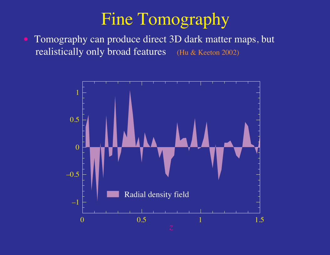
Fine Tomography• Tomography can produce direct 3D dark matter maps, but realistically only broad features (Hu & Keeton 2002)

Radial density field

1

0.5

0

–0.5

–1

0 0.5 1 1.5z

Fine Tomography• Tomography can produce direct 3D dark matter maps, but realistically only broad features (Taylor 2002; Hu & Keeton 2002)

Radial density fieldWiener reconstruction

1

0.5

0

–0.5

–1

0 0.5 1 1.5z

Fine Tomography• Tomography can produce direct 3D dark matter maps, but realistically only broad features (Taylor 2002; Hu & Keeton 2002)

Radial density fieldWiener reconstruction

1

0.5

0

–0.5

–1

0 0.5 1 1.5z

Fine Tomography• Tomography can produce direct 3D dark matter maps, but realistically only broad features (Hu & Keeton 2002)

Radial density fieldWiener reconstruction

1

0.5

0

–0.5

–1

0 0.5 1 1.5z

Fine Tomography• Tomography can produce direct 3D dark matter maps, but realistically only broad features (Hu & Keeton 2002)

Radial density fieldWiener reconstruction

1

0.5

0

–0.5

–1

0 0.5 1 1.5z

Growth Function• Localized constraints (fixed distance-redshift relation)

4000 sq. deg

z0.5 1 1.5 2

windows

1.4

1.2

1.0

0.8

0.6

0.60.40.2

mtot=0.2eV

Hu (2002) 3 degenerate mass ν's assumed e.g. Beacom & Bell (2002)

z0.5 1 1.5 2

1.5

1.0

0.5

0.50

-0.5

ρ DE/

ρ cr0

windows

w=–0.8

Dark Energy Density• Localized constraints (with cold dark matter)

Hu (2002)

4000 sq. deg

Dark Energy Parameters• Three parameter dark energy model (ΩDE, w, dw/dz=w')

Hu (2002)

1

0.5-0.9

-1

-1.1

0

-0.5

0.6 0.65 0.7-1

ΩDE0.6 0.65 0.7

ΩDE

w'

w

σ(ΩDE)=0.01

σ(w')=0

0.03

nonenone

4000 sq. deg.

Lensing of a Gaussian Random Field• CMB temperature and polarization anisotropies are Gaussian

random fields – unlike galaxy weak lensing

• Average over many noisy images – like galaxy weak lensing

Lensing by a Gaussian Random Field• Mass distribution at large angles and high redshift in

in the linear regime

• Projected mass distribution (low pass filtered reflectingdeflection angles): 1000 sq. deg

rms deflection2.6'

deflection coherence10°

Lensing in the Power Spectrum• Lensing smooths the power spectrum with a width ∆l~60

• Convolution with specific kernel: higher order correlations between multipole moments – not apparent in power

Pow

er

10–9

10–10

10–11

10–12

10–13

lensedunlensed

∆power

l10 100 1000

Seljak (1996); Hu (2000)

Reconstruction from the CMB• Correlation betweenFourier momentsreflectlensing potentialκ = ∇2φ

〈x(l)x′(l′)〉CMB = fα(l, l′)φ(l + l′) ,

wherex ∈ temperature, polarization fieldsandfα is a fixed weightthat reflects geometry

• Each pair forms anoisy estimateof the potential or projected mass- just like a pair of galaxy shears

• Minimum variance weightall pairs to form an estimator of thelensing mass

Quadratic Reconstruction• Matched filter (minimum variance) averaging over pairs of

multipole moments

• Real space: divergence of a temperature-weighted gradient

Hu (2001)

originalpotential map (1000sq. deg)

reconstructed1.5' beam; 27µK-arcmin noise

Ultimate (Cosmic Variance) Limit• Cosmic variance of CMB fields sets ultimate limit

• Polarization allows mapping to finer scales (~10')

Hu & Okamoto (2001)

100 sq. deg; 4' beam; 1µK-arcmin

mass temp. reconstruction EB pol. reconstruction

Matter Power Spectrum• Measuring projected matter power spectrum to cosmic vari-

ance limit across whole linear regime 0.002< k < 0.2 h/Mpc

Hu & Okamoto (2001)

10 100 1000

10–7

10–8

defle

ctio

n po

wer

"Perfect"

Linear

Lσ(w)∼0.06

∆P

P≈ −0.6

(mtot

eV

)

Matter Power Spectrum• Measuring projected matter power spectrum to cosmic vari-

ance limit across whole linear regime 0.002< k < 0.2 h/Mpc

Hu & Okamoto (2001)

10 100 1000

10–7

10–8

defl

ectio

n po

wer

"Perfect"Planck

Linear

Lσ(w)∼0.06; 0.14

Summary• Gravitational lensing is the only direct probe of the dark sector: composition of dark matter: massive neutrinos nature of the dark energy: scalar field? Λ?

• With sources distributed in redshift, tomography possible• Coarse radial resolution sufficient for recoving linear growth rate dark energy density evolution• Requires good photometric redshifts, elimination of systematics, avoidance of intrinsic alignment contamination

• CMB provides ultimate high-z source for tomography; precision neutrino constraints in principle possible