econstorMake Your Publications Visible.

A Service of

zbwLeibniz-InformationszentrumWirtschaftLeibniz Information Centrefor Economics

Lehmann, Etienne; Marical, François; Rioux, Laurence

Working Paper

Labor income responds differently to income-tax andpayroll-tax reforms

CESifo Working Paper, No. 3974

Provided in Cooperation with:Ifo Institute – Leibniz Institute for Economic Research at the University of Munich

Suggested Citation: Lehmann, Etienne; Marical, François; Rioux, Laurence (2012) : Laborincome responds differently to income-tax and payroll-tax reforms, CESifo Working Paper, No.3974, Center for Economic Studies and ifo Institute (CESifo), Munich

This Version is available at:http://hdl.handle.net/10419/66564

Standard-Nutzungsbedingungen:

Die Dokumente auf EconStor dürfen zu eigenen wissenschaftlichenZwecken und zum Privatgebrauch gespeichert und kopiert werden.

Sie dürfen die Dokumente nicht für öffentliche oder kommerzielleZwecke vervielfältigen, öffentlich ausstellen, öffentlich zugänglichmachen, vertreiben oder anderweitig nutzen.

Sofern die Verfasser die Dokumente unter Open-Content-Lizenzen(insbesondere CC-Lizenzen) zur Verfügung gestellt haben sollten,gelten abweichend von diesen Nutzungsbedingungen die in der dortgenannten Lizenz gewährten Nutzungsrechte.

Terms of use:

Documents in EconStor may be saved and copied for yourpersonal and scholarly purposes.

You are not to copy documents for public or commercialpurposes, to exhibit the documents publicly, to make thempublicly available on the internet, or to distribute or otherwiseuse the documents in public.

If the documents have been made available under an OpenContent Licence (especially Creative Commons Licences), youmay exercise further usage rights as specified in the indicatedlicence.

www.econstor.eu

Labor Income Responds Differently to Income-Tax and Payroll-Tax Reforms

Etienne Lehmann François Marical Laurence Rioux

CESIFO WORKING PAPER NO. 3974 CATEGORY 1: PUBLIC FINANCE

OCTOBER 2012

An electronic version of the paper may be downloaded • from the SSRN website: www.SSRN.com • from the RePEc website: www.RePEc.org

• from the CESifo website: Twww.CESifo-group.org/wp T

CESifo Working Paper No. 3974

Labor Income Responds Differently to Income-Tax and Payroll-Tax Reforms

Abstract We estimate the responses of gross labor income with respect to marginal and average net-of-tax rates in France over the period 2003-2006. We exploit a series of reforms to the income-tax and payroll-tax schedules affecting individuals who earn less than twice the minimum wage. Our estimate for the elasticity of gross labor income with respect to the marginal net-of-income-tax rate is around 0.2, while we find no response to the marginal net-of-payroll-tax rate. The elasticity with respect to the average net-of-tax rate is not significant for the income-tax schedule, while it is close to -1 for the payroll-tax schedule. A plausible explanation is the existence of significant labor supply responses to the income-tax schedule, combined with sticky posted wages (i.e., the gross labor income minus payroll taxes divided by hours worked). Finally, the effect of the net-of-income-tax rate seems to be driven by participation decisions, in particular those of married women.

JEL-Code: H240, H310, J220, J380.

Keywords: labor income, payroll tax, income tax.

Etienne Lehmann CREST – INSEE

92245 Malakoff Cedex / France etienne.lehmann@ensae.fr

François Marical

INSEE 92245 Malakoff Cedex / France

francois.marical@insee.fr

Laurence Rioux CREST – INSEE

92245 Malakoff Cedex / France laurence.rioux@insee.fr

October 16, 2012 We are grateful to the editor Wojciech Kopczuk, two anonymous referees, Valérie Albouy, Soren Blomquist, Richard Blundell, Clément Carbonnier, Bart Cockx, Bruno Crépon, Laurence Jacquet, Henrik Kleven, Camille Landais, Guy Laroque, Andreas Peichl, Thomas Piketty, Alain Trannoy, Bruno Van der Linden and participants in seminars at CREST, PSE-Jourdan, IRES, French Ministry of the Economy, the CESifo workshop on “Taxation, transfers and the labour market”, the LAGV 2011 conference, the Tinbergen Institute conference 2011 on “Friction and Policy” and the IZA Workshop “Recent Advances in Labor Supply Modeling” for their helpful remarks and comments. We thank Richard Crabtree for editing this manuscript. Remaining errors are ours. The data was accessed through the CASD dedicated to researchers and authorized by the French “Comité du secret statistique”.

2

I. Introduction

Labor income taxation is composed of several distinct schedules. According to the OECD,1 the

total tax wedge for an average-wage worker amounted to 29.7% of employers’ labor costs in the U.S.

in 2010. This tax wedge can be decomposed into 8.2% for transfers to the “central government”, 5.8%

for “sub-central” governments, and 15.8% for “social security contributions”. In France at the same

time, the total tax wedge for an average-wage earner amounted to 49.3%, with 9.9% for transfers to

the central government and 39.3% for social security contributions. Whether or not labor income

responds identically to the different schedules is crucial for determining which type of tax should be

used to finance public expenditure, including social security and redistribution. In this work, we focus

on the relative responsiveness of labor income to payroll taxation (social security contributions, in

France) versus income taxation.

Most of usual models of the labor market (including the standard labor supply model, the

monopoly union model under the right-to-manage, or the individual wage-bargaining model) predict

identical income responses to payroll-tax and income-tax schedules. By contrast, the empirical

evidence is so far not conclusive because the existing literature never considers the responses to

payroll taxes and income taxes at the same time, due to the absence of simultaneous reforms to both

schedules for similar individuals over the same period. 2

In contrast to the literature, we exploit a series of reforms to both income-tax and payroll-tax

schedules that occurred in France over 2003-2006 in the bottom half of the labor income distribution.

In 2003, there existed two distinct schedules for the reduction in employers’ payroll taxes for low-

wage workers, depending on whether the firm had moved to the 35-hour workweek or remained at 39

hours. A progressive convergence between the two schedules was implemented from 2003 and

completed in July 2005. This resulted in opposite effects for the two types of firms: an increase in the

reduction in employers’ payroll taxes for those remaining at 39 hours (hereafter the “39-hour firms”)

and a decrease in the reduction for those that had moved to the 35-hour week (hereafter the “35-hour

firms”). Over the same period, the Prime pour l’Emploi, a working tax credit for low-wage earners,

was substantially increased, the maximum amount of benefits being almost doubled between 2003 and

2006. Exploiting this rich set of reforms that affected workers earning less than twice the minimum

wage gives us the very rare opportunity to compare the responsiveness of labor income to income-tax

and payroll-tax reforms.

1 Authors’ calculations from the OECD tax database at http://www.oecd.org/dataoecd/44/3/1942514.xls 2 Most of the papers focus on the distortions induced by income taxes (e.g. Feldstein (1995), Auten and Carroll (1999), Gruber and Saez (2002), Saez (2003), Blomquist and Selin (2010), Cabannes, Houdré and Landais (2011) among others. Another strand of the literature estimates the effects of payroll-tax reforms (e.g. Gruber (1997), Kugler and Kugler (2009), Liebman and Saez (2006), and Saez, Matsaganis and Tsakloglu (2012b) among others).

3

The dataset we use is the Enquête Revenus Fiscaux, which combines income tax records from

the fiscal administration with the French Labor Force Survey (hereafter LFS). We use income tax

records to compute the income tax schedule (including the tax credit for low-wage earners). The LFS

provides the additional variables we need to reconstruct employer and employee payroll taxes. In

particular, we use the labor market history and the usual weekly working time to obtain a monthly

labor income and a wage rate, which are both necessary to compute payroll taxes over the period we

consider. We are also able to infer whether the firm has moved to the 35-hour week or remained at 39

hours, which determines which payroll tax schedule applies. Using this dataset that matches income

tax records with the LFS enables us to investigate the responsiveness to both income-tax and payroll-

tax reforms.

More precisely, we estimate the short-term responses of gross labor income (labor income

inclusive of employer and employee payroll taxes, i.e., total labor cost) to the marginal and average

net-of-tax rates3 for both schedules. We find a significant elasticity (around 0.2) of gross labor income

with respect to the marginal net-of-income-tax rate. By contrast, the elasticity of gross labor income

with respect to the marginal net-of-payroll-tax rate is found to be not significant and close to zero.

Gross labor income thus responds differently to payroll-tax changes and to income-tax changes, at

least in the short-run, which is in contradiction with the theoretical predictions of the most common

labor market models. We also find that the income effects of payroll-tax and income-tax changes are

different. The elasticity with respect to the average net-of-payroll-tax rate does not differ significantly

from minus one, while the elasticity with respect to the average net-of-income-tax rate is lower and

generally non-significant but varies across sub-samples. Our results are robust to the specification of

pre-reform income controls.

Our preferred interpretation for these findings is significant labor supply responses to the

income-tax schedule, combined with the stickiness of posted wage rates (i.e., the gross labor income

minus payroll taxes divided by hours worked). The effects of an income-tax reform operate through

rapid labor supply modifications. Further investigations indicate that these responses are essentially

due to the participation decisions of married women. By contrast, posted wage rates are determined

largely through the minimum wage and collective bargaining in France. Our findings suggest that

these institutions fail to respond to payroll-tax changes, at least over the three-year period we consider.

Our results also suggest that, at least in the short-run, financing social security expenses and

redistribution through payroll taxes is less distortive than through income taxes.

A large strand of the literature studies the response of taxable income (i.e. income net of tax

deductions) to the marginal net-of-income-tax rate, following the idea of Lindsey (1987) and Feldstein

(1995) that this elasticity summarizes all the deadweight losses due to taxation. We here detail our

contributions to this literature. i) Our first contribution concerns the way of controlling for income

3 The marginal (respectively average) net-of-tax rate is equal to one minus the marginal (average) tax rate.

4

effects. While the literature following Gruber and Saez (2002) identifies income effects by controlling

for actual changes in virtual incomes, we do so by including changes in the average net-of-tax rate

computed for a labor income fixed at its initial value. We argue that this method is more consistent

with the theoretical framework. This also leads to robust estimates across empirical specifications. ii)

Our 0.2 estimate of the gross labor income elasticity with respect to the marginal net-of-income-tax

rate lies between 0.12 and 0.4, which is the plausible interval for the elasticity of taxable income

according to Saez et alii (2012a). It is also close to the 0.33 intensive margin elasticity of Chetty

(2012). Here, however, we estimate the response of labor income, while most works study the

response of taxable total income, which includes tax avoidance behavior and (some of) capital income

responses. Restricting the comparison to labor income, our estimate is consistent with that of

Blomquist and Selin (2010), who find significant responses of 0.2 for men in Sweden, and with that of

Saez (2003), who obtains an elasticity of around 0.1 for the US, although his estimates do not

significantly differ from 0. Our estimate is higher than the narrow interval of 0.05-0.12 obtained by

Kleven and Schultz (2012) for labor income responses in Denmark. iii) The existing literature suggests

that the elasticity is presumably much higher for top income earners (e.g., Gruber and Saez (2002)).

However, we obtain a significant elasticity of labor income with respect to the marginal net-of-

income-tax rate by using reforms that affect individuals in the bottom half of the wage distribution. iv)

Our result that labor income is, at least in the short-run, insensitive to the marginal payroll-tax rate is

consistent with those found by other studies on payroll taxation (e.g., Liebman and Saez (2006), Saez

et alii (2012b)). More specifically for France, it is in line with Aeberhardt and Sraer (2009), who find

that the reduction in employers’ payroll tax for low-wage workers did not generate wage moderation

(see also L’hommeau and Remy (2009) and Bunel, Gilles, and L’Horty (2012)).

The paper is organized as follows. In section II, we detail the institutional backgrounds and

expose the main reforms that took place in France over the 2003-2006 period. Section III presents the

theoretical framework and discusses whether labor income should respond identically to income taxes

and to payroll taxes. In section IV, we present our empirical strategy and discuss the identification.

Section V describes the dataset used, which combines income tax records with the Labor Force

Survey. Section VI presents results for the respective effects of payroll taxes and income taxes on

gross labor income for all employees and for specific subsamples, and the last section concludes.

II. Institutional background

We here describe the reforms to the payroll-tax and income-tax schedules that occurred in France

during the 2003-2006 period.

5

II.1 Income tax reforms

We use the term “income tax” to denote both the income tax per se and a tax credit for low-

paid earners (Prime pour l’emploi, hereafter PPE). Income tax per se in France is calculated at the

fiscal household level, which differs from the usual notion of household: two persons who live as a

couple are considered by the administration as a single fiscal household only if they are married or

linked by a civil pact. The income-tax schedule is a function of the ratio of total income earned by the

fiscal household to the weighted sum (parts fiscales) of its members. The amount of tax paid then

equals the income tax that would be paid by a single individual whose income is equal to this ratio,

divided by the weighted sum. This implies that both the marginal and average net-of-tax tax rates of a

given individual change with marital status, spouse’s income, the birth of a child, or the departure of

adult children. These events are likely to affect labor supply decisions, the only exception being the

departure of an adult child which generates an instantaneous change in the tax schedule, while the

change in the labor supply, if any, is likely to be smoothed over time. Therefore, income tax reforms

provide more convincing sources of identification than these family events. Nevertheless, thanks to the

complexity of the tax schedule, the very large range of income tax rates that different individuals with

similar incomes can face improves the identification possibilities.

Over the 2003 – 2006 period covered by our dataset, there are several changes in the income

tax code per se. In 2004 and 2005, tax brackets were indexed to consumer price inflation. This

generated a form of “bracket creep” (Saez (2003)), as labor incomes increased slightly more rapidly

than inflation over this period. A more substantial reform in 2006 reduced the number of brackets

from seven to five and modified the rates.

However, the reform that generated the largest changes in tax rules over 2003-2006 was the

increase in the Prime pour l’Emploi, a tax credit conditional on working that had been created in 2001.

Both eligibility for the tax credit and the amount paid depend essentially on the individual full-time

equivalent annual labor income, but the total income earned by the household and the household’s

composition also intervene. More precisely, a single worker without children is eligible provided that

her annual labor income is above 0.3 and her full-time equivalent annual labor income is below 1.4

times the annual minimum wage (up to 2.1 times the annual minimum wage for some household

compositions). One-third of French employees are eligible for the working tax credit.4 We now

describe the scheme for a single individual without children working full-time.5 If she does not work a

4 In France in 2006, 22% of the employed earn a wage between 0.3 and 1.4 times the minimum wage, and 50% earn a wage between 0.3 and 2.1 times the minimum wage. Compared to the EITC or the WFTC, the French tax credit thus differs on two points: a much larger share of the population is eligible, and the presence of children has a very limited effect on the amount of benefit. 5 If she works part-time, the tax credit is computed as a function of the hourly wage, but the tax credit is more advantageous for each hour of work than if she works full-time. This bonus for part-time workers has increased over the period studied, providing an additional source of identification.

6

full year and is paid the minimum wage, she is eligible for a phase-in range between 0.3 and 1 times

the annual minimum wage where the tax credit is proportional to the wage. If she works the full year,

unlike the EITC in the US, there is no plateau range: the tax credit is maximized at the minimum wage

and the phase-out range extends from 1 to 1.4 times the annual minimum wage. Entering the phase-in

income range leads to a reduction in both marginal and average tax rates. Entering the phase-out

income range is associated with a rise in the marginal tax rate, since a higher labor income reduces the

tax credit. The average tax rate is minimal at the minimum wage level and then increases. While the

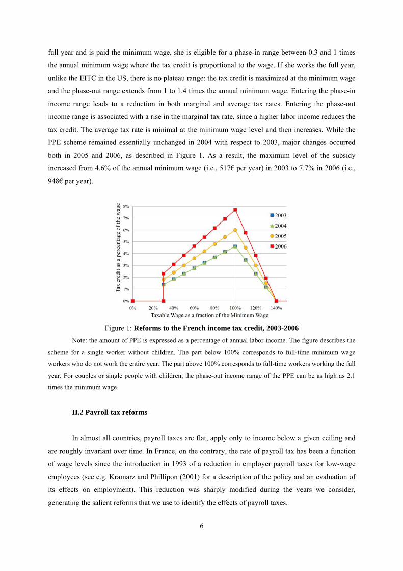
PPE scheme remained essentially unchanged in 2004 with respect to 2003, major changes occurred

both in 2005 and 2006, as described in Figure 1. As a result, the maximum level of the subsidy

increased from 4.6% of the annual minimum wage (i.e., 517€ per year) in 2003 to 7.7% in 2006 (i.e.,

948€ per year).

Figure 1: Reforms to the French income tax credit, 2003-2006

Note: the amount of PPE is expressed as a percentage of annual labor income. The figure describes the

scheme for a single worker without children. The part below 100% corresponds to full-time minimum wage

workers who do not work the entire year. The part above 100% corresponds to full-time workers working the full

year. For couples or single people with children, the phase-out income range of the PPE can be as high as 2.1

times the minimum wage.

II.2 Payroll tax reforms

In almost all countries, payroll taxes are flat, apply only to income below a given ceiling and

are roughly invariant over time. In France, on the contrary, the rate of payroll tax has been a function

of wage levels since the introduction in 1993 of a reduction in employer payroll taxes for low-wage

employees (see e.g. Kramarz and Phillipon (2001) for a description of the policy and an evaluation of

its effects on employment). This reduction was sharply modified during the years we consider,

generating the salient reforms that we use to identify the effects of payroll taxes.

7

The reforms to the employer payroll tax reduction for low-wage employees over 2003-2006

were a consequence of the introduction of the 35-hour workweek. In June 1998, a law implemented by

a left-wing government initiated the move to a 35-hour workweek, a process that became in principle

mandatory for large firms (more than 20 employees) in January 2000 and for small firms in January

2002. This process towards the 35-hour workweek generated two sets of minimum wage regulations6

and two payroll tax reduction schedules. Firms moving from a 39-hour to a 35-hour workweek were

given an additional reduction in employer payroll taxes compared with those remaining on 39 hours,

in order to facilitate and accelerate the move to the 35-hour workweek. As all firms were intended to

move to the 35-hour workweek, the existence of two types of tax subsidies was viewed as no more

than a transitional issue at that time. However, in June 2002 a right-wing government came into power

and stopped the 35-hour reform. A non-negligible proportion of firms had not adopted the 35-hour

workweek at that time and had no intention of doing so later (Table 1). In January 2003, a law was

passed providing for the convergence towards a common reduction schedule for both 35-hour and 39-

hour firms. The convergence process lasted two and a half years and was completed in July 2005.

Bunel et alii (2012) provide a complete description of the reform and an evaluation of its employment

effects.

Figure 2 presents the changes in the tax subsidy during the period of observation, from 2003 to

2006, for the two types of firms. At the beginning, in January 2003, the two subsidy schedules differed

substantially. For a 39-hour firm (solid curve), the reduction in employer payroll taxes reached a

maximum of 18.2 percentage points at the hourly minimum wage, and then decreased up to 1.3 times

the minimum wage. For a 35-hour firm (dashed curve), the reduction reached a maximum of 26

percentage points at 1.076 times the hourly minimum wage, then decreased up to 1.937 times the

minimum wage.7 For the 39-hour firms, the maximum reduction increased from 18.2 percentage

points in 2003 to 26 in 2006. Moreover, the phase-out income range widened from 1-1.3 times the

minimum wage to 1-1.6 times the minimum wage. For the 35-hour firms, the maximum percentage

points of reduction remained unchanged, while the phase-out income range of the subsidy shifted to

the left, from 1.076-1.937 times the minimum wage in 2003 to 1-1.6 times the minimum wage in

2006. On average over the period 2003-2006, the tax subsidy decreased for 35-hour firms while it

increased for 39-hour firms.

6 To prevent the workweek reduction from lowering the monthly labor income, the (hourly) minimum wage regulation (SMIC for Salaire Minimum Interprofessionnel de Croissance) was supplemented by a system of monthly guaranteed wages (GMR for Guarantie Mensuelle de Rémunerations), which depended on the date at which the firm adopted the 35-hour workweek. 7 In 2003, for a firm having adopted the 35-hour workweek in 2000, the monthly guaranteed wage (GMR) was equal to 1.076 times the minimum wage. The reduction was maximal at the GMR level and decreased up to 1.8 times the GMR, i.e., 1.937 times the minimum wage.

8

Figure 2: Changes in the reduction in employer payroll taxes for low paid earners, 2003-2006

These reforms induced up-and-down movements in marginal and average tax rates, depending

on the type of firms and on whether the wage rate was below or above 1.6 times the minimum wage.

We use this rich set of changes in marginal and average payroll tax rates in the bottom half of the

income distribution to identify gross labor income responses to payroll taxation. However, two points

are worth mentioning. First, as the reforms only affected employer payroll taxes, leaving employee

payroll taxes unchanged, we cannot disentangle the responses to employer and to employee payroll

taxes. Second, as future retirement and unemployment benefits are not affected by the payroll tax

reduction, we cannot analyze the behavioral response to payroll taxes regarding whether or not the

reform also affects workers’ future benefits.

III. Theoretical background

III.1 Definitions and concepts

Because of taxes and transfers, the net labor income c that a worker consumes and the gross

labor income w that her employer pays are different. Labor income taxation is composed, on the one

hand, of social security contributions or payroll taxes (which finance social security programs such as

PAYG pensions, health insurance, unemployment insurance, etc.) and, on the other hand, of taxes to

governments or income taxes. The payroll tax is represented as a function of the gross labor income.

The posted labor income z is defined as the gross labor income net of (employer and employee)

payroll taxes.8 On a linear part of the payroll tax schedule with a marginal net-of-payroll-tax rate τP

8 Our definition of posted income differs from Saez et alii (2012b), where it is taken to be gross labor income net of employer payroll tax, but inclusive of employee payroll tax. In contrast with Saez et alii for Greece, there was no reform to employee payroll taxes in France over our observation period, implying that the effects of employee

9

and a virtual posted income RP, the posted labor income verifies z = τP w + RP. We denote by

ρP = z/w = τP + RP/w the average net-of-payroll-tax rate. The income tax schedule consists of income

tax per se and of tax credits providing income subsidies to low-wage earners. The income tax is a

function of the posted labor income z. On a linear part of the income tax schedule with a marginal net-

of-income-tax rate τI and a virtual net income RI, the net labor income c is given by c=τI z + RI. We

denote by ρI = c/z = τI + RI/z the average net-of-income-tax rate. The budget constraint can be written:

IPIPI RRwc ++= τττ (1)

The three labor incomes w, z and c are endogenous and may depend on each of the four tax

parameters τI, τP, RI and RP. Assuming that the gross labor income w is determined by a behavioral

function denoted W(τI,τP,RI,RP), we get:

w

R

R

W

w

R

R

WW

w

W

ww

w I

I

P

PI

I

I

I

p

P

P

P Δ

∂∂+Δ

∂∂+Δ

∂∂+Δ

∂∂=Δ

ττ

ττ

ττ

ττ

(2)

The uncompensated payroll tax elasticity (τP/w)(∂W/∂τP) captures the percentage change in the

gross labor income after a payroll tax reform that increases the marginal net-of-payroll-tax rate by one

percent, while decreasing the amount of payroll tax paid by 0.01 w*, where w* denotes the pre-reform

gross labor income. The literature on optimal taxation, however, is more interested in the compensated

elasticity, which is the relevant elasticity for computing deadweight losses. A compensated payroll tax

reform is defined as a simultaneous change in the marginal net-of-payroll-tax rate ΔτP and in the

virtual posted income ΔRP, such that the amount of payroll tax paid at the initial gross labor income w*

remains unchanged. Symmetrically, we are interested in the sensitivity of gross labor income to a

compensated income tax reform, i.e., to a simultaneous change in the marginal net-of-income-tax rate

ΔτI and in the virtual net income ΔRI, which leaves unchanged the amount of income tax paid at the

initial gross labor income w*. Let P

τβ and I

τβ denote the elasticities of gross labor income with

respect to a compensated payroll tax reform and to a compensated income tax reform. Equation (2) can

be rewritten as (see Appendix A.1):

I

II

P

PP

I

II

P

pP

w

w

ρρβ

ρρβ

ττβ

ττβ ρρττ

Δ+Δ+Δ+Δ=Δ

(3)

payroll taxes are empirically not identifiable. Consequently, we do not need to distinguish theoretically between employer and employee payroll taxes.

10

In Equation (3), PρΔ =ΔτP + ΔRP / w* denotes the change in the average net-of-payroll-tax rate while

IρΔ =ΔτI + ΔRI / z* - (RI/z*) PρΔ /ρP denotes the change in the average net-of-income-tax rate, both

being computed while keeping the gross labor income fixed at its initial value w*. Except when gross

labor income is unresponsive to tax reforms or when taxation is proportional, the changes PρΔ and

IρΔ for a constant gross labor income differ from the actual changes ΔρP and ΔρI which are affected

by the responses of gross labor income.9

Our way of controlling for income effects thus differs from what is usually done in the

literature since Gruber and Saez (2002). For ease of comparison, let us leave aside payroll taxation for

a moment. Our main departure from the standard procedure comes from our inclusion of the change in

average net-of-tax rates computed for the unchanged gross labor income w*, while the literature

includes the actual change. Equation (3) shows that controlling for income effects by including the

actual change in the average net-of-tax rate erroneously adds to the right-hand side a term that depends

on the dependent variable Δw/w.

Another difference with the literature is that we include the change in the average net-of-tax

rate instead of the change in after-tax income. The two procedures are equivalent when the changes in

average net-of-tax rate and after-tax income are computed while keeping pre-reform gross labor

income unchanged.10 When actual changes are considered, the two procedures differ, except under

proportional taxation. If the tax schedule is close to proportional, controlling income effects by the

after-tax income instead of the average net-of-tax rate is of little importance. Since proportional

taxation is a good approximation for top-income earners, the standard procedure is acceptable when

evaluating the behavioral responses in the top of the distribution. This is no longer true when

estimating the elasticities in the bottom half of the distribution, since the existence of tax credit for

low-income earners implies that the tax schedule is far from being proportional in this part of the

distribution.11

9 Using ρP = τP + RP/w, the actual change in the average net-of-payroll-tax rate is equal to: ΔρP = ΔτP + ΔRP/w -

ρP Δw/w = PρΔ - (RP/w*) Δw/w. This gives: ΔρP/ρP = PρΔ /ρP - (RP/z*) Δw/w. Symmetrically, the

differentiation of ρI = τI + RI/(ρP w) implies that: ΔρI = ΔτI + ΔRI / z* - (RI/z*) (ΔρP/ρP + Δw/w) = ΔτI + ΔRI/z* -

(RI/z*) PρΔ /ρP – (1-(RP/z*)) (RI/z*) Δw/w, which finally leads to: ΔρI/ρI = PρΔ /ρP – (1-(RP/z*)) (RI/c*) Δw/w.

Under proportional taxation, RI=RP=0, implying that IρΔ =ΔρI and PρΔ =ΔρP.

10 The log change in after-tax income is then equal to (Δτ w + ΔR)/(τ w + R) = ( ρΔ w)/(ρ w) = ρΔ /ρ. 11 A last difference is that we theoretically define (see Equation (A3) of Appendix A.1) the income response parameter as the product of the derivative of the gross income with respect to a marginal transfer to the average net-of-tax rate, while Gruber and Saez (2002) define it as the product of the same derivative to the marginal net-of-tax rate. As marginal net-of-tax rates are slightly lower than average net-of-tax rates, our income response effect is slightly higher. If their estimates, associated with the actual change in after-tax incomes, coincide with their theoretical definition of the income effects, this is due to several approximations that are only valid under proportional taxation (see their footnote 3).

11

III.2 Benchmark labor market models

In a large class of labor market models, the gross labor income (or labor cost) is determined by

the maximization of an objective function that depends negatively on the gross labor cost w to the firm

and positively on the net labor income c paid to the worker. This objective takes the general form

U(c,w) with 'w

'c UU >> 0 . We henceforth refer to this class of models as the “benchmark” ones.

The textbook labor supply framework is typically one of these. In it, a worker of productivity

p supplying L units of labor earns a gross income w = p L. If her preferences over consumption and

labor supply are described by the utility function u(c,L), with 'L

'c uu >> 0 , one can define function U

by U(c,w) ≡ u(c,w/p). Choosing the labor supply L amounts to choose the gross labor income w = p L.

The objective U is here decreasing in the gross labor income w, because earning a higher gross labor

income w requires the worker to work harder (i.e., higher L).12

The monopoly union model (under right-to-manage) is also a benchmark model (Hersoug

(1984)). If the union’s objective over net labor income c and employment L is described by u(c,L) and

labor demand is described by the decreasing function L=ld(w), then the function U is defined by

U(c,w) ≡ u(c,ld(w)). Here, U is decreasing in gross labor income because the labor demand depends

negatively on the labor cost w. Lastly, wage bargaining settings (e.g. Lockwood and Manning (1993),

Pissarides (2000)) are other examples of benchmark models. In these frameworks, function U(c,w) is

given by the generalized Nash product where the worker’s (or union’s) contribution to the Nash

product is increasing in the net labor income c, while the firm’s contribution is decreasing in w, as

higher gross labor incomes reduce profits. However, it is worth noting that for both the monopoly

union model and the wage bargaining model, the objective function takes the form U(c,w) only if the

wage setting concerns homogeneous workers and firms, which implies that the wage and tax schedules

are unique. Hence, only bargaining models at the individual level (e.g. Mortensen and Pissarides

(1994)) or at the collective level but for homogenous labor markets can be reduced to the

maximization of this type of objective.

In any of these “benchmark” models, the gross labor income w is determined by the

maximization of U(c,w) subject to the budget constraint (1), i.e., ( ) ( )RwRwUw w ,,maxarg ττ Ω≡+= .

In this program, the posted income z being economically irrelevant, the various tax parameters

influence the gross labor income only through the global marginal net-of-tax rate, τ = τI τP, and the

global virtual income, R=τI RP + RI. The behavioral function thus takes the form Ω(τI τP,τI RP + RI) ≡

12 It worth noting that in this model, if we leave aside payroll taxation, the compensated elasticity I

τβ

corresponds to the Hicksian labor supply elasticity, which depends only on substitution effects, while the uncompensated elasticity (τI/w)(∂W/∂τI) corresponds to the Marshallian labor supply elasticity, which depends on both substitution and income effects.

12

W(τI,τP,RI,RP). We show that this restriction implies identical elasticities for income taxation and

payroll taxation (see Appendix A.2):

Pτβ =

Iτβ > 0 and P

ρβ = Iρβ (4)

The second-order condition, together with the assumption that the objective U is increasing in c,

ensures that jτβ are positive for j=I, P. Moreover, in the labor supply framework, assuming in addition

the normality of leisure implies that jρβ are negative for j=I, P.

III.3 Alternatives models

Prediction (4) is obtained in the very large class of benchmark models. Therefore, if estimating

Equation (3) leads us to reject this prediction, we need to look for alternative frameworks that can

account for such departures. We have three alternatives in mind that we now describe separately.

Obviously, these alternatives are not mutually exclusive.

Difference in salience

The "salience" (in the sense of Chetty, Looney, and Kroft (2009)) of income-tax reforms and

of payroll-tax reforms may be different. For instance, one could argue that, since payroll taxes are paid

on a monthly basis while income taxes are paid on an annual basis with a one-year lag in France, labor

income should react more rapidly to changes in payroll taxes than to changes in income taxes. In this

case, Iτβ and I

ρβ are expected to have the same sign but to be lower in absolute terms than Pτβ and P

ρβ

respectively. Conversely, one might argue that individuals are much more aware of the income tax

schedule than of the payroll tax schedule. This implies that Iτβ and I

ρβ should have the same sign but

be larger in absolute terms than Pτβ and P

ρβ respectively. A difference in salience would therefore

imply either:

PIττ ββ <<0 and PI

ττ ββ < (5)

or:

IPττ ββ <<0 and

IPρρ ββ < (6)

13

Deferred benefits

Payroll taxes finance various social programs. For some of them, both the eligibility and the

benefit level are related to the amount of payroll taxes paid. The most illustrative example is the

pension system, where the level of pension received depends explicitly on both the level and duration

of contributions. Unemployment insurance also exhibits this contribution-related property: in the event

of job loss, the maximum duration of UI benefits depends on the duration of contributions. When

payroll taxes per se generate deferred benefits with some probability, the objective to be maximized

must be modified by adding a function of the level of payroll taxes into consumption. Therefore, the

gross labor income solves:

( ) ( )( )( )wRwkRwURRWw PPw

PIIP ,1maxarg,,, −−++== ττττ (7)

In this specification, the parameter k captures how the overall level of consumption depends

on the level of payroll taxes (1-τP)w + RP through the deferred payments of various benefits. Different

arguments suggest that k is small. First, as the level of deferred benefits depends on the whole labor

market history (in particular for pensions), current contributions only partially determine this level.

Second, deferred benefits will only be given in the future, and with some probability, which generates

discounting. We hence assume that k < τI and k < ρI. Appendix A.3 shows that the elasticity with

respect to the marginal (average) net-of-payroll-tax rate is lower (lower in absolute terms) than the

elasticity with respect to the marginal (average) net-of-income-tax rate, because part of the tax is now

considered as a gain in consumption. We thus obtain Prediction (6) instead of Prediction (4).

Posted wage rate stickiness

Finally, consider again the labor supply model where individuals have preferences u(c,L) over

consumption c and labor supply L, but assume now that the posted wage rate (denoted s) is sticky.

This assumption echoes the finding of Saez et alii (2012b) for Greece, that employer payroll taxes are

entirely borne by employers. This is also plausible in France, where collective wage setting, for

instance through collective wage bargaining or minimum wage regulation, applies to a large

proportion of workers and specifies posted wage rates. Under posted wage rate stickiness, a worker

supplying L units of labor receives the posted income z=sL. She thus chooses her labor supply to

maximize U(c,z) =u(c,z/s), taking her posted wage rate s as given. Therefore, the posted labor income

does not depend on the payroll tax parameters, implying that:

14

I

II

I

II

z

z

ρρβ

ττβ ρτ

Δ+Δ=Δ (8)

instead of (3). Instead of Prediction (4), posted wage rates stickiness leads to:13

0=Pτβ and

1−=Pρβ (9)

IV. Empirical strategy

Our objective is to evaluate jointly the responses of gross labor income to income-tax and

payroll-tax reforms. In specifying the empirical setup, we are aware that heterogeneous individuals

may respond to tax changes differently. Hence, we only provide evidence on the average of these

behavioral elasticities, i.e. on the Local Average Treatment Effect (LATE). We estimate the following

empirical counterpart of Equation (3) for an individual i employed at t-1 and t:

titiIti

IPti

PIti

IPti

Pti uXw ,1,,,,,, logloglogloglog +⋅+Δ+Δ+Δ+Δ+=Δ −γρβρβτβτβα ρρττ (10)

where Δ is the time-difference operator between dates t and t-1, Xi,t-1 is a vector of observed individual

and firm characteristics measured in the base period (i.e. t-1), and ui,t is an error term that captures

unobserved and time-varying heterogeneity. Our specification differs from the canonical model à la

Gruber and Saez (2002) in the way income effects are controlled for. According to Equation (3) in

section III, we include the log change in average net-of-tax rates, computed while keeping the real

gross labor income fixed at its pre-reform value,14 instead of the actual log change in virtual income.

More specifically, let πt-1 be the average growth rate of gross labor income between years t-1 and t, and

let 11,1, −−− ×= ttiti ww π denote the base-year inflation-adjusted gross labor income. For j=P,I,

( )1,

1,,

;1

−

−−=ti

tijj

ti w

twTρ is the average net-of-tax rate obtained by applying the year-t tax rule to the year t-

1 adjusted gross income. Income effects are captured by the inclusion of jti

jti

jti 1,,, logloglog −−=Δ ρρρ .

13 Under posted wage rates stickiness, there is no loss of generality in computing changes in average tax rates while keeping the posted income z* (instead of the gross income w*) unchanged at its initial value. From z = ρ

w, we get Δw/w=Δz/z - ΔρP/ρP=Δz/z - p

ρΔ /ρP.

14 Since payroll taxation in France is actually a function of the posted income and not of the gross income, we approximate the changes in tax rates for a constant gross income by the changes in tax rates for a constant posted income.

15

Various methodological issues complicate the estimation. A first issue concerns the potential

simultaneity bias. Because of the nonlinearity of the payroll-tax and the income-tax schedules

respectively, the marginal net-of-tax rates Pti,τ and I

ti,τ are functions of the gross labor income level.

To isolate the impact of taxes on gross labor income, we need instruments for jti,logτΔ , with j=P,I. In

the literature, the standard procedure, proposed by Auten and Carroll (1999), uses the predicted change

in the log of the net-of-tax rate should the real labor income not change from year t-1 to year t. By

construction, the instrument captures changes in the tax rate in the absence of any behavioral response.

We apply this method to the marginal net-of-tax rates associated with the two tax schedules. For j=P,I,

we define ( )

w

twT tij

jti

∂∂−= − ;

1 1,,τ . The “type-I” instrument for the change in the log of the marginal

net-of-tax rates is then given by: jti

jti

jti 1,,, logloglog −−=Δ τττ . Note that

jti,log ρΔ , included in our

specification to control for income effects, would be the type-I instrument for the average net-of-tax

rate if we had followed the literature in considering actual changes in average net-of-tax rates. It does

not need to be instrumented since, by construction, it does not depend on the behavioral change in tiw , .

Another issue concerns the existence of non-tax related changes in gross labor income. These

changes can be specific to income groups. For example, technical progress and international trade

generate changes in gross labor income, which are likely to be different across firm size and industry,

age category, level of education, etc., and presumably lead to a widening of the wage distribution

(Gruber and Saez (2002)). The risk when evaluating a tax reform that reduces the marginal tax rate for

top income earners, such as TRA86 in the U.S., is to attribute changes in gross labor income to the

reform rather than to these “non-tax” causes, thereby causing an upward bias in the elasticity estimate.

Reversion to the mean constitutes another source of non-tax factors. An individual with an unusually

low (respectively high) labor income in period t-1 is very likely to have a higher (lower) one at t. This

is typically what happens when an individual enters unemployment (or involuntary part-time work)

during year t-1. Her labor income is then unusually low and increases substantially in year t if she

finds a permanent (or full-time) job. These non-tax related changes in gross labor income imply that

the base-year income is correlated with the error term whenever ui,t is not a white noise process

(Holmlund and Söderström (2008), Blomquist and Selin (2010), Weber (2011)). To control for

reversion to the mean and trends in the gross wage distribution, the standard procedure in the literature

is to include a function of base-year income, f(log wi,t-1), in the vector of controls Xi,t-1. Auten and

Carroll (1999) use a linear function, while Gruber and Saez (2002) propose a flexible 10-piece spline.

However, as pointed out by Kopczuk (2005), mean reversion and heterogeneous income trends across

income groups are two separate phenomena, and it is unlikely that a function of base-year income

alone can capture both effects. Kopczuk (2005) thus proposes to include two separate variables: a 10-

piece spline of the log difference between base-year income and income in the preceding year, log(wi,t-

16

1)-log(wi,t-2), to account for mean reversion and other transitory income effects, and a 10-piece spline

of the gross labor income in the year preceding the base year, log(wi,t-2), to control for heterogeneous

shifts in the income distribution. Since our dataset provides information on gross labor income in year

t-2, we follow the latter strategy in our baseline specification.

However, if the residual remains correlated with the base year income despite the inclusion of

the two sets of spline, type-I instruments and the change in average net-of-tax rates may be

endogenous, since they are functions of base-year income. We then propose a second group of

instruments based on year t-2 gross labor income. Let 122,2, −−−− ××= tttiti ww ππ and

22,2, −−− ×= ttiti ww π denote the t-2 gross labor income inflation-adjusted for years t and t-1, where

2−tπ denotes the average growth rate of gross labor income between years t-2 and t-1. We then define,

for j =P, I:

( ) ( )( ) ( )

2,

2,1,

2,1,

2,

2,,

2,,

1;1and

1;1

;1and

;1

−

−−

−−

−

−−

−−=∂

−∂−=

−=∂

∂−=

ti

tijj

titi

jjti

ti

tijj

titi

jjti

w

twT

w

twT

w

twT

w

twT

ρτ

ρτ

Using the above definitions, type-II instruments for j=P,I are given by jti

jti

jti 1,,, logloglog −−=Δ τττ

and jti

jti

jti 1,,, logloglog −−=Δ ρρρ . Type-II instruments are valid provided that the residual follows a

MA(1) process.

The issue of controlling for the effects of pre-reform income is particularly relevant when the

tax reform used is targeted to high-income earners, as in most US studies. In this case, by construction,

jti,logτΔ is correlated with log(wi,t-1), which biases the estimates if the residuals are auto-correlated,

despite the presence of pre-reform income controls (Weber (2011)). For instance, Kopczuk (2005)

illustrates how sensitive the estimates of taxable income elasticity for the US are to the specification of

pre-reform income controls. This issue is less severe when changes in marginal tax rates are not

systematically correlated with pre-reform income. For instance, tax reforms in Denmark in the 1980s

concern the whole income distribution; inside income-groups, they increase the marginal tax rate for

some individuals while decreasing it for others. Indeed, Kleven and Shultz (2012) using Danish data

find much more robust estimates than Kopczuk (2005) using US data. As the French tax reforms we

use generate up-and-down movements in marginal tax rates that are nonlinear functions of pre-reform

income (see Section II), we expect the issue of controlling for the effects of pre-reform income to be

less severe than in US studies (see our robustness checks in Section VI.2).

We consider several specifications that differ in the set of instruments used, the variables

included to control for non-tax related changes in gross labor income and the set of covariates. Our

preferred specification includes a 10-piece spline of the log of t-2 income to control for divergence in

17

the income distribution and a 10-piece spline in the deviation to control for mean reversion, and uses

both instruments I and II.

V. The data

The existing empirical literature uses either administrative income tax records (e.g. Feldstein

(1995), Auten and Carroll (1999), Gruber and Saez (2002)) or payroll tax records (e.g. Saez et alii

(2012b)). Although administrative tax records have the advantage of providing exhaustive and

longitudinal data, they contain limited information on individual characteristics and no information on

labor market history and firms’ characteristics. Since the main goal for collecting these data is policy-

oriented, only the variables necessary to compute taxes are provided. In contrast to the existing

literature, we use a research-oriented dataset, the Enquête Revenus Fiscaux (hereafter ERF), produced

by matching the French Labor Force Survey with administrative income tax records. The LFS is a

rotating 18-month panel that starts a new 18-month wave every quarter. Individuals interviewed at the

4th quarter of year-t in the LFS are matched with their year-t administrative income tax records to

generate the year-t wave of the ERF dataset. As individuals are interviewed during six consecutive

quarters, they are at best present during two consecutive years in the ERF dataset. We use the 2003-

2006 waves of the ERF because reforms to both the payroll-tax and income-tax schedules occurred

during this period for similar individuals. The individuals sampled thus appear either in 2003 and

2004, in 2004 and 2005, or in 2005 and 2006. As the LFS contains detailed information on personal

characteristics (in particular education), labor market history and job characteristics (in particular usual

weekly hours of work, industry), we are able to control in a rich way for mean reversion and for other

trends in the gross labor income distribution.

We now describe the labor income variable we use. The year-t administrative income tax

records report, for each member of the household, the annual posted labor income (which corresponds

to the gross income minus payroll taxes) earned at dates t-2, t-1 and t. The variable is reported by the

employer and controlled by the fiscal administration, and as such is reliable. We are then able to

compute the income tax rate very precisely using a tax simulator adapted from the INES (INsee Etudes

Sociales) micro-simulation model provided by INSEE and DREES.

Employer and employee payroll taxes are paid each month and are calculated as a function of

the monthly posted labor income. Employer payroll taxes are also based on the posted wage rate,

through the tax subsidy for low-wage employees.15 In addition, employer and employee payroll taxes

depend on the firm size,16 the type of work,17 and whether or not the firm has adopted the 35-hour

15 The employer payroll tax subsidy for low-wage employees is described in detail in section II. 16 The payroll tax schedule distinguishes between firms with less than 10 employees, those with between 10 and 20, and those with more than 20.

18

workweek. Although we have no record of actual payroll taxes, our dataset (through the LFS) contains

the information necessary to reconstruct payroll taxes by applying the legislation. We thus proceed in

this way and build our own payroll tax calculator. The monthly posted labor income is computed as

the annual amount (drawn from tax records) divided by the number of months of work reported in the

LFS; the posted wage rate is calculated using the usual weekly hours of work also reported in the LFS.

Two types of measurement errors can intervene. First, the LFS is a self-declared survey and as such

may be less precise than the tax records we use to compute the income tax rate. Second, in the LFS,

the workers are not directly asked to report whether they work in a 35-hour firm or a 39-hour firm. A

natural way to detect those working in a 35-hour firm is to use the information on the usual weekly

hours of work: we thus consider that employees whose usual weekly working time is at most 35 hours

in full-time equivalent are employed in 35-hour firms. Moreover, the working time reduction has also

been implemented through the granting of additional days off (jours de Réduction du Temps de

Travail, hereafter RTT days). In the LFS, workers are asked to report whether they benefit from RTT

days. We thus consider that those who declare they benefit from RTT days work in 35-hour firms. We

are sure that workers who declare either that they benefit from those additional days off or that they

usually work 35 hours a week are indeed employed in 35-hour firms. There may remain a

measurement error for those supposed to work in 39-hour firms, since workers may omit to declare in

the LFS that they benefit from RTT days. Consequently, we expect to be more precise when restricting

our sample to 35-hour workers and, on the contrary, to be less precise on the sub-sample of the

workers supposed to work in 39-hour firms. To limit the measurement error on the working time

regulation, we restrict the sample to employees who work either in a 35-hour firm at t and t-1 or in a

39-hour firm at both dates.18

We compute the payroll and income taxes at date t and simulate the effects of a 5% increase in

labor income to obtain marginal net-of-tax rates. As administrative tax records also provide

information on the posted labor income at t-1 and t-2, we are able to compute our two types of

instruments: instrument I based on wi,t-1 and instrument II based on wi,t-2. We restrict the sample to

individuals who experienced no change in their marital status between dates t-1 and t, since those who

marry, divorce, or become widowed have to make several tax returns. In addition, we exclude public

sector workers, as they are subject to very specific labor market regulations, and the self-employed.

Finally, we restrict the sample to employees who report a positive labor income at dates t-2, t-1 and t.

Our final sample comprises 12,512 individuals observed over two consecutive years.

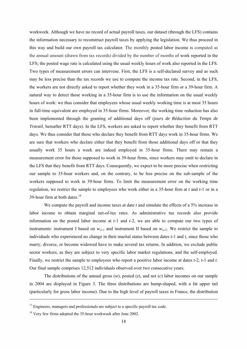
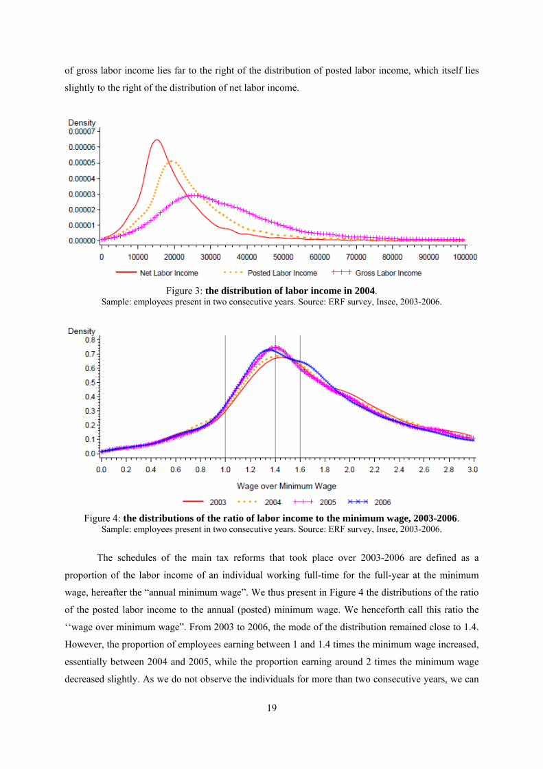
The distributions of the annual gross (w), posted (z), and net (c) labor incomes on our sample

in 2004 are displayed in Figure 3. The three distributions are hump-shaped, with a fat upper tail

(particularly for gross labor income). Due to the high level of payroll taxes in France, the distribution

17 Engineers, managers and professionals are subject to a specific payroll tax code. 18 Very few firms adopted the 35-hour workweek after June 2002.

19

of gross labor income lies far to the right of the distribution of posted labor income, which itself lies

slightly to the right of the distribution of net labor income.

Figure 3: the distribution of labor income in 2004. Sample: employees present in two consecutive years. Source: ERF survey, Insee, 2003-2006.

Figure 4: the distributions of the ratio of labor income to the minimum wage, 2003-2006. Sample: employees present in two consecutive years. Source: ERF survey, Insee, 2003-2006.

The schedules of the main tax reforms that took place over 2003-2006 are defined as a

proportion of the labor income of an individual working full-time for the full-year at the minimum

wage, hereafter the “annual minimum wage”. We thus present in Figure 4 the distributions of the ratio

of the posted labor income to the annual (posted) minimum wage. We henceforth call this ratio the

‘‘wage over minimum wage”. From 2003 to 2006, the mode of the distribution remained close to 1.4.

However, the proportion of employees earning between 1 and 1.4 times the minimum wage increased,

essentially between 2004 and 2005, while the proportion earning around 2 times the minimum wage

decreased slightly. As we do not observe the individuals for more than two consecutive years, we can

20

hardly determine whether these shifts in the income distribution reflect behavioral responses to tax

reforms or changes in the characteristics of the different samples across time.

Age Economic activity < 20 years 0.1 % Agriculture 1.5 % 20 - 29 years 13.4 % Manufacturing 26.8 % 30 - 39 years 29.4 % Construction 7.2 % 40 - 49 years 33.4 % Energy 1.6 % 50 - 59 years 22.9 % Education and social activities 9.9 % ≥ 60 years 0.8 % Trade and repair 17.0 % Gender Other tertiary 35.9 % Women 42.1 % Job tenure Men 57.9 % < 1 year 5.8 % Household composition 1 - 5 years 25.4 % Single individual 11.1 % 5 - 10 years 18.6 % Single parent 6.3 % ≥ 10 years 50.0 % Couples without children 20.3 % Firm size Couples with children 59.5 % < 10 employees 13.6 % Other households 2.8 % 10-19 employees 7.0 % Change in the number of children ≥ 20 employees 79.4 % Birth of a child between t and t-1 5.5 % 35-hour workweek 76.0 % Departure of a child between t and t-1

6.2 % 35-hour workweek and < 20 employees 8.6 %

No change 88.3 % 35-hour workweek and ≥ 20 employees 67.4 % Level of education College (> 2 years) 11.1 % College (≤ 2 years) 17.5 % High school graduate 16.0 % High-school drop-out or vocational diploma 38.3 % Junior high school or basic vocational 7.5 % No diploma or elementary school 9.6 % N° observations 12 512

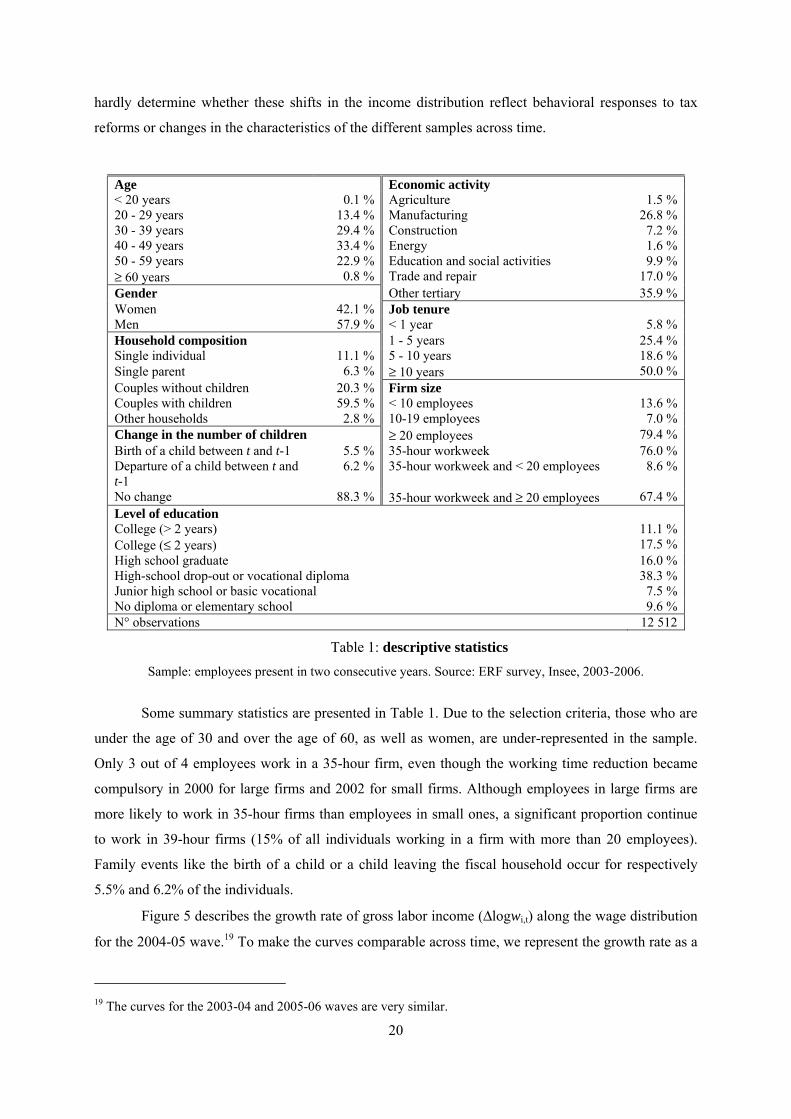
Table 1: descriptive statistics

Sample: employees present in two consecutive years. Source: ERF survey, Insee, 2003-2006.

Some summary statistics are presented in Table 1. Due to the selection criteria, those who are

under the age of 30 and over the age of 60, as well as women, are under-represented in the sample.

Only 3 out of 4 employees work in a 35-hour firm, even though the working time reduction became

compulsory in 2000 for large firms and 2002 for small firms. Although employees in large firms are

more likely to work in 35-hour firms than employees in small ones, a significant proportion continue

to work in 39-hour firms (15% of all individuals working in a firm with more than 20 employees).

Family events like the birth of a child or a child leaving the fiscal household occur for respectively

5.5% and 6.2% of the individuals.

Figure 5 describes the growth rate of gross labor income (Δlogwi,t) along the wage distribution

for the 2004-05 wave.19 To make the curves comparable across time, we represent the growth rate as a

19 The curves for the 2003-04 and 2005-06 waves are very similar.

21

function of the wage over minimum wage ratio. Given the variability of growth rates among

individuals with the same income level, we compute the means within each percentile of the posted

labor income for each year. Figure 5 displays the reversion-to-the-mean phenomenon at the bottom

end of the wage distribution. The most plausible explanation for this fact is exit from

unemployment/entry into stable employment between years t-1 and t.

Figure 5: means of the growth rate of gross labor income for each percentile of the distribution of labor income in 2004

Sample: employees present in two consecutive years. Source: ERF survey, Insee, 2003-2006.

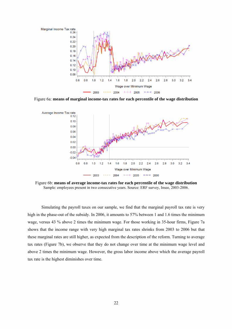
Figures 6a and 6b depict the evolution of marginal 1-τI and average 1-ρI income-tax rates

simulated on our sample over the years 2003-2006. Although the rates are very noisy, especially for

part-time workers below the full-time minimum wage, for each year we observe that the marginal rate

is much higher between 1 and 1.4 times the annual minimum wage than elsewhere. Moreover, as

expected, the increase in the tax credit from 2003 to 2006 leads to a significant rise in the marginal

income-tax rate in this phase-out range. It also reduces the average income-tax rate, especially at the

minimum wage level where the PPE is maximal. The tax reforms generated by the income-tax per se,

on the contrary, are much less apparent, except for the reduction in the average tax rate between 2005

and 2006 for gross labor income above two times the annual minimum wage.

22

Figure 6a: means of marginal income-tax rates for each percentile of the wage distribution

Figure 6b: means of average income-tax rates for each percentile of the wage distribution Sample: employees present in two consecutive years. Source: ERF survey, Insee, 2003-2006.

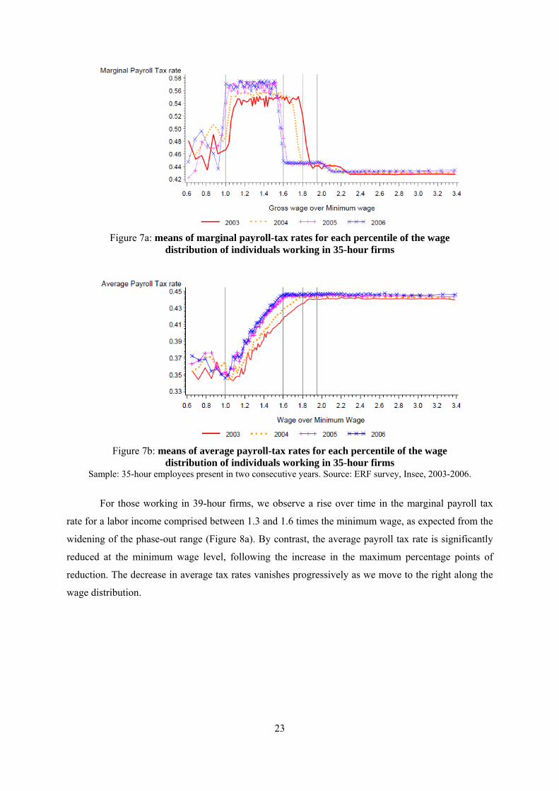
Simulating the payroll taxes on our sample, we find that the marginal payroll tax rate is very

high in the phase-out of the subsidy. In 2006, it amounts to 57% between 1 and 1.6 times the minimum

wage, versus 43 % above 2 times the minimum wage. For those working in 35-hour firms, Figure 7a

shows that the income range with very high marginal tax rates shrinks from 2003 to 2006 but that

these marginal rates are still higher, as expected from the description of the reform. Turning to average

tax rates (Figure 7b), we observe that they do not change over time at the minimum wage level and

above 2 times the minimum wage. However, the gross labor income above which the average payroll

tax rate is the highest diminishes over time.

23

Figure 7a: means of marginal payroll-tax rates for each percentile of the wage distribution of individuals working in 35-hour firms

Figure 7b: means of average payroll-tax rates for each percentile of the wage distribution of individuals working in 35-hour firms

Sample: 35-hour employees present in two consecutive years. Source: ERF survey, Insee, 2003-2006.

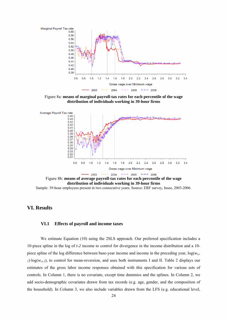
For those working in 39-hour firms, we observe a rise over time in the marginal payroll tax

rate for a labor income comprised between 1.3 and 1.6 times the minimum wage, as expected from the

widening of the phase-out range (Figure 8a). By contrast, the average payroll tax rate is significantly

reduced at the minimum wage level, following the increase in the maximum percentage points of

reduction. The decrease in average tax rates vanishes progressively as we move to the right along the

wage distribution.

24

Figure 8a: means of marginal payroll-tax rates for each percentile of the wage distribution of individuals working in 39-hour firms

Figure 8b: means of average payroll-tax rates for each percentile of the wage

distribution of individuals working in 39-hour firms Sample: 39-hour employees present in two consecutive years. Source: ERF survey, Insee, 2003-2006.

VI. Results

VI.1 Effects of payroll and income taxes

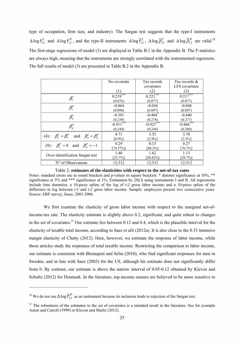
We estimate Equation (10) using the 2SLS approach. Our preferred specification includes a

10-piece spline in the log of t-2 income to control for divergence in the income distribution and a 10-

piece spline of the log difference between base-year income and income in the preceding year, log(wi,t-

1)-log(wi,t-2), to control for mean-reversion, and uses both instruments I and II. Table 2 displays our

estimates of the gross labor income responses obtained with this specification for various sets of

controls. In Column 1, there is no covariate, except time dummies and the splines. In Column 2, we

add socio-demographic covariates drawn from tax records (e.g. age, gender, and the composition of

the household). In Column 3, we also include variables drawn from the LFS (e.g. educational level,

25

type of occupation, firm size, and industry). The Sargan test suggests that the type-I instruments

Iti,logτΔ and P

ti,logτΔ , and the type-II instruments Iti,logτΔ , I

ti,log ρΔ and Pti,log ρΔ are valid.20

The first-stage regressions of model (3) are displayed in Table B.1 in the Appendix B. The F-statistics

are always high, meaning that the instruments are strongly correlated with the instrumented regressors.

The full results of model (3) are presented in Table B.2 in the Appendix B.

No covariate

(1)

Tax records covariates

(2)

Tax records & LFS covariates

(3) I

τβ 0.219*** 0.221*** 0.217***

(0.076) (0.077) (0.077)

Pτβ -0.064 -0.036 -0.048

(0.098) (0.097) (0.097) Iρβ -0.391 -0.484* -0.440

(0.239) (0.278) (0.277) Pρβ -0.911*** -0.923*** -0.866***

(0.244) (0.244) (0.260)

PIPIρρττ ββββ == and:)4( 4.71 3.55 3.70

[0.9%] [2.9%] [2.5%]

1and0:)9( −== PPρτ ββ 0.29 0.13 0.27

[74.57%] [88.2%] [76.7%]

Over-identification Sargan test 1.40 1.62 1.13 [23.7%] [20.42%] [28.7%]

N° of Observations 12,512 12,512 12,512

Table 2: estimates of the elasticities with respect to the net-of-tax rates Notes: standard errors are in round brackets and p-values in square brackets. * denotes significance at 10%, ** significance at 5% and *** significance at 1%. Estimation by 2SLS using instruments I and II. All regressions include time dummies, a 10-piece spline of the log of t-2 gross labor income and a 10-piece spline of the difference in log between t-1 and t-2 gross labor income. Sample: employees present two consecutive years. Source: ERF survey, Insee, 2003-2006.

We first examine the elasticity of gross labor income with respect to the marginal net-of-

income-tax rate. The elasticity estimate is slightly above 0.2, significant, and quite robust to changes

in the set of covariates.21 Our estimate lies between 0.12 and 0.4, which is the plausible interval for the

elasticity of taxable total income, according to Saez et alii (2012a). It is also close to the 0.33 intensive

margin elasticity of Chetty (2012). Here, however, we estimate the response of labor income, while

those articles study the responses of total taxable income. Restricting the comparison to labor income,

our estimate is consistent with Blomquist and Selin (2010), who find significant responses for men in

Sweden, and in line with Saez (2003) for the US, although his estimate does not significantly differ

from 0. By contrast, our estimate is above the narrow interval of 0.05-0.12 obtained by Kleven and

Schultz (2012) for Denmark. In the literature, top-income earners are believed to be more sensitive to

20 We do not use Pti,logτΔ as an instrument because its inclusion leads to rejection of the Sargan test.

21 The robustness of the estimates to the set of covariates is a standard result in the literature. See for example Auten and Carroll (1999) or Kleven and Shultz (2012).

26

taxes than those in the rest of the distribution, in particular because they can more easily benefit from

avoidance opportunities (e.g. Gruber and Saez (2002)). Our results show that significant responses

may also arise for low or median-income individuals, who were the most affected by the tax reforms

of 2003-2006 in France.

Conversely, our estimate for the effect of marginal net-of-payroll-tax rates on gross labor

income Pτβ is close to zero and not significant, whatever the set of controls included. The result that

gross labor income does not respond to marginal payroll tax rates suggests that, at least in the short

run, the efficiency costs of financing social security expenses and redistribution are lower through

payroll taxes than through income taxes. This finding is in line with Saez et alii (2012b) for Greece,

and with Aeberhardt and Sraer (2009) for France. However, it differs from that of Lhommeau and

Remy (2009), also for France, who find that the progressivity of payroll taxes has a slight negative

effect on wage growth. Although these last two studies are based on the same data set, Lhommeau and

Remy (2009) use data aggregated at the firm level and Aeberhardt and Sraer (2009) use individual

data, which may account for the difference in findings. Bunel et alii (2012), who evaluate the 2003-

2005 French reform in payroll tax reductions, find a positive but small impact on average labor

income. Note that they evaluate the global effect of the reform and do not disentangle the changes in

payroll tax progressivity and the changes in average tax rates.

We now turn to income effects. The elasticity with respect to the average net-of-income-tax

rate is negative but not significant (it is only significant at the 10% level in Column 2), which is in line

with the literature (e.g. Gruber and Saez (2002)). By contrast, the elasticity with respect to the average

net-of-payroll-tax rate is negative and significant. The parameter is not very sensitive to the set of

covariates included, since it varies between -0.92 and -0.86. More importantly, we cannot reject that it

is equal to -1, which suggests that labor income is negotiated net of employer payroll taxes. A

decrease in employer payroll taxes seems almost entirely absorbed by employers and thus actually

reduces the labor cost, without any significant effect on the posted wage rate.

Our result that gross labor income is insensitive to marginal payroll tax rates but responds to

marginal income tax rates has important implications. Section III described how a large class of

theoretical models of the labor market predicts identical elasticities, as expressed by Prediction (4).

This class includes the textbook labor supply model where the gross wage rate equals the marginal

productivity of labor. According to the F-tests, the evidence for France is that Prediction (4) is strongly

rejected (at the 1% level for Model (1) and at the 5% level for Models (2) and (3)).

Moreover, we find that gross labor income responds more to marginal net-of-income-tax rates

than to marginal net-of-payroll-tax rates, but less to average net-of-income-tax rates than to average

net-of-payroll-tax rates. This leads us to reject the assumption of a difference in salience between

payroll tax and income tax (Predictions (5) and (6)). This also leads us to reject models where payroll

27

taxes generate deferred benefits that are internalized in the formation of gross labor income (Prediction

(6)).

We test Prediction (9) that the elasticity of gross labor income with respect to the marginal

net-of-payroll-tax rate is equal to zero whereas the elasticity with respect to the average net-of-payroll-

tax rate is equal to -1. This prediction is obtained when posted wage rates are sticky. The F-tests

indicate that Prediction (9) is easily accepted by the data. In France, wages are largely determined

through collective bargaining. Collective wage agreements occur at both industry and firm levels and

concern three-quarters of workers each year (Avouyi-Dovi, Fougère and Gautier (2011)). If

negotiations at the industry level occur frequently, negotiations at the firm level concern less than one

quarter of workers each year. This point is important because the decision to move to the 35-hour

workweek is taken at the firm level. As a result, the wage response to the change in payroll taxes is

slowed down by the low frequency of wage bargaining at the firm level. In addition, collective

bargaining at the industry level involves 35-hour firms and 39-hour firms. Both types of firms have

been subjected to very different payroll tax changes, which significantly limits the wage response at

the industry level. Furthermore, what is negotiated is the posted wage rate (not the gross wage rate).

As the reform to the payroll tax reduction we use here only affects employer payroll taxes, it is not

surprising that posted wage rates did not react quickly to those reforms. Our finding thus suggests that

in France, collective wage bargaining fails to respond to payroll-tax changes, at least over the three-

year period we consider.

VI.2 Robustness checks

We now conduct a sensitivity analysis. An important departure of our paper from the literature

on taxable income elasticity lies in the way we control for income effects. We include the changes in

average net-of-tax rates computed for a constant labor income pρΔ /ρP and I

ρΔ /ρI, while the literature

following Gruber and Saez (2002) includes the actual changes in virtual income (see Section III).

Table 3 explores the consequences of this departure. Column 1 reproduces our benchmark

specification. In Column 2, there is no control for the income effects. The gross labor income

elasticities with respect to the marginal net-of-tax rates are very close to those in Column (1).

Moreover, the hypothesis IPττ ββ = of identical responses to income taxes and payroll taxes, which

corresponds to Prediction (4) in the absence of income effects, is rejected at the 5% level. In Column

(3), we control for the actual changes in average net-of-tax rates ΔρP/ρP and ΔρI/ρI instead of the

changes for a constant labor income pρΔ /ρP and I

ρΔ /ρI. This has a very limited impact on the

elasticities Iτβ and P

τβ with respect to the marginal net-of-tax rates. The impact is stronger on the

elasticity Iρβ with respect to the average net-of-income-tax rate, which becomes significantly negative

28

and larger in magnitude. The elasticity Pρβ with respect to the average net-of-payroll-tax rate also

grows in magnitude, but remains very close to -1. Overall, Prediction (4) of identical responses to

income taxes and payroll taxes is still rejected, while Prediction (9) associated with posted wage rate

stickiness is even more easily accepted.

In Column (4), we control for income effects by including actual changes in virtual income.22

The effect on the estimates is dramatic, except for the elasticity with respect to the marginal net-of-

payroll-tax rate which remains insignificant and close to zero. The other elasticities Iτβ , P

τβ and Pρβ

now have the wrong sign. In Section III, we theoretically argued that controlling for actual changes

(Columns 3 and 4) erroneously adds to the right-hand side of Equation (10) a term that depends on the

dependent variable Δw/w. Actual changes in average net-of-tax rates are, however, close to changes in

after-tax rates for a constant labor income whenever taxation is close to proportional. The bias due to

using actual changes in average net-of-tax rates in Column (3) is thus minor. Conversely, even under

proportional taxation, actual changes in virtual income are different from changes in virtual income for

a constant labor income. Then, the bias due to using actual changes in Column (4) is more serious and

we thus do not consider the specification of Column (4) to be consistent.

Benchmark specification

(1)

No control

(2)

Actual changes in average net of tax

rates (3)

Actual changes in virtual incomes

(4)

Iτβ 0.217*** 0.214*** 0.267*** -0.283*

(0.077) (0.077) (0.076) (0.157) P

τβ -0.048 -0.027 0.007 0.012 (0.097) (0.097) (0.089) (0.108)

Iρβ -0.440 -0.823** 0.384*

(0.277) (0.332) (0.184) Pρβ -0.866*** -1.083*** 2.026***

(0.260) (0.282) (0.484)

PIPIρρττ ββββ == and:)4( 3.70 5.10 3.90 9.92

[2.5%] [2.4%] [2.3%] [0.0%]

1and0:)9( −== PPρτ ββ 0.27 0.05 19.6

[76.7%] [95.4%] [0.0%]

Over-identification Sargan test 1.13 0.75 3.62 3.84 [28.7%] [38.7%] [30.45%] [27.8%]

N° of Observations 12,512 12,512 12,512 12,512

Table 3: elasticities for different ways of controlling for income effects Notes: standard errors are in round brackets and p-values in square brackets. * denotes significance at 10%, ** significance at 5% and *** significance at 1%. Estimation by 2SLS using instruments I and II. All regressions include ERF and LFS covariates, a 10-piece spline of the log of t-2 gross labor income and a 10-piece spline of the difference in log between t-1 and t-2 gross labor income. Sample: employees present in two consecutive years. Source: ERF survey, Insee, 2003-2006.

22 It is worth reminding here that changes in virtual income for a constant labor income are equal to changes in average net-of-tax rates for a constant labor income.

29

Table 4 provides robustness checks with respect to the specification of pre-reform income

controls and to the instrumentation. Column (1) reproduces our benchmark specification with 10-piece

splines of log(wi,t-2) and of the deviation, and both types of instruments. In Column (2), we use only

type-I instruments, which implies that pρΔ /ρP and I

ρΔ /ρI are taken as exogenous. Columns (3), (4)

and (5) propose alternative specifications for pre-reform income levels: a linear function of log(wi,t-1)

as in Auten and Carroll (1999) in Column (3); a 10-piece spline of log(wi,t-1) as in Gruber and Saez

(2002) in Column (4), and linear functions of log(wi,t-2) and of log(wi,t-1)-log(wi,t-2) in Column (5). The

last of these follows the suggestion of Kopczuk (2005) to disentangle transitory income effects and

heterogeneous shifts in the income distribution. Finally, Column (6) extends the baseline specification

by allowing the splines to be different for 35-hour and 39-hour employees. This specification is

motivated by the different evolution of the minimum wage regulation for the two types of firms,

thereby generating different trends for the lowest income across the two subsamples.

The estimates for the effects of marginal tax rates are robust across specifications of pre-

reform income controls. The elasticity of gross labor income with respect to the marginal net-of-

income-tax rate varies between 0.17 and 0.35 and is always statistically significant, whereas the

response to the marginal net-of-payroll-tax rate is never significantly different from zero. The

elasticity with respect to the average net-of-payroll-tax rate is always significant but more sensitive to

the specification, since it varies between -0.5 and -1.27. The response to the average net-of-income-tax

rate is the parameter whose estimation is the least robust. It is significant and high in magnitude in

Columns (3) and (5), while it does not significantly differ from zero in the other specifications.

Comparing Column (3) to Column (4) and Column (5) to Column (2) thus stresses the importance of

allowing for potential nonlinear effects of base-year income when evaluating the effects of average

net-of-tax rates.

The robustness of our results across specifications, at least for the effects of marginal net-of-

tax rates, echoes the findings of Kleven and Shultz (2012) for Denmark, whereas it contrasts

significantly with those presented by Kopczuk (2005) for the US. Like the Danish tax reforms and

unlike the US ones, the French tax reforms we use generate many up-and-down movements in tax

rates that are not systematically correlated with the pre-reform income, which may contribute to the

robustness of our results. Furthermore, the way we control for income effects using changes in average

net-of-tax rates for constant labor income instead of actual changes in virtual income also help to

improve the robustness of our results.

30

Benchmark specification

(1)

Benchmark specification - type-I instruments

(2)

Linear function of log(wi,t-1) - type-I

instruments (3)

Iτβ 0.217*** 0.209*** 0.355***

(0.077) (0.077) (0.082) P

τβ -0.048 -0.048 -0.014 (0.097) (0.097) (0.103)

Iρβ -0.440 -0.301 -1.492***

(0.277) (0.203) (0.298) Pρβ -0.866*** -1.061*** -0.937***

(0.260) (0.227) (0.280)

PIPIρρττ ββββ == and:)4( 3.70 5.85 6.10

[2.5%] [0.3%] [0.2%]

1and0:)9( −== PPρτ ββ 0.27 0.15 0.02

[76.7%] [86.3%] [98.3%]

Over-identification Sargan test 1.13 * * [28.7%]

N° of Observations 12,512 12,512 12,512

10-piece spline of log(wi,t-1) - type-I

instruments

(4)

Linear functions of log(wi,t-2) and of

Δlog(wi,t-1) - type-I instruments

(5)

Splines of log(wi,t-2) and of Δlog(wi,t-1)) that are

different for 35-hour and 39-hour employees

(6) I

τβ 0.174** 0.336*** 0.213***

(0.077) (0.081) (0.078) P

τβ -0.166 0.006 -0.033(0.102) (0.101) (0.117)

Iρβ

-0.221 -1.201*** -0.478*

(0.209) (0.294) (0.278) Pρβ

-1.269*** -0.499* -0.894*

(0.232) (0.275) (0.537) PIPIρρττ ββββ == and:)4(

10.23 5.90 2.40[0.0%] [0.3%] [9.1%]

1and0:)9( −== PPρτ ββ

1.88 1.66 0.07

[15.2%] [19.0%] [93.4%]

Over-identification Sargan test * * 1.46 [22.7%]

N° of Observations 12,512 12,512 12,512

Table 4: elasticities for different controls of base-year income Notes: standard errors are in round brackets and p-values in square brackets. * denotes significance at 10%, ** significance at 5% and *** significance at 1%. Estimation by 2SLS. All regressions include ERF and LFS covariates. Sample: employees present in two consecutive years. Source: ERF survey, Insee, 2003-2006.

VI.3 Heterogeneous effects

We now investigate the robustness of our estimates across various subsamples, which will

help us to clarify the economic mechanisms behind our results. First, as mentioned in Section II, those

working in 35-hour firms and those working in 39-hour firms were subjected to very different payroll

tax changes (Figure 2). The tax subsidy was reduced for 35-hour firms but increased for 39-hour ones.

To check the robustness of our main result that labor income responds differently to income taxes and

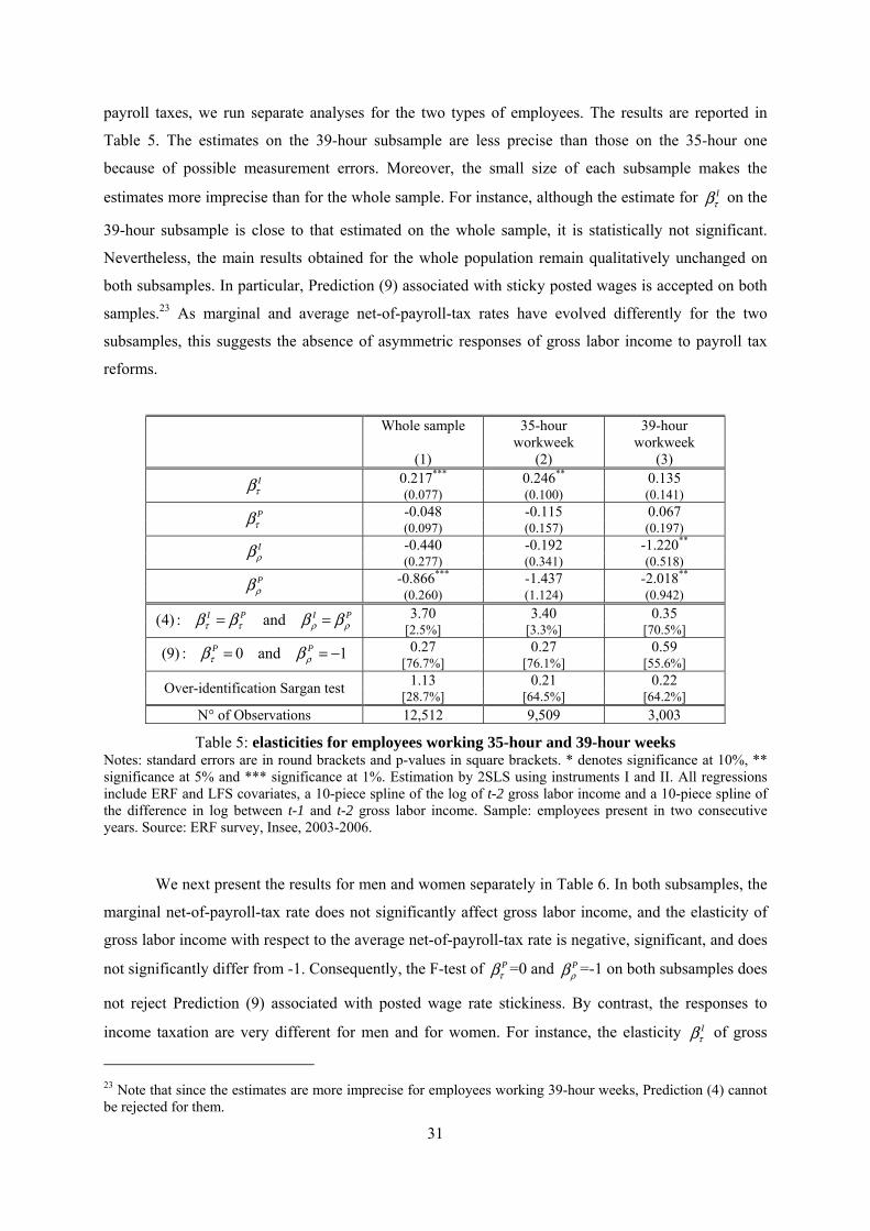
31

payroll taxes, we run separate analyses for the two types of employees. The results are reported in

Table 5. The estimates on the 39-hour subsample are less precise than those on the 35-hour one

because of possible measurement errors. Moreover, the small size of each subsample makes the

estimates more imprecise than for the whole sample. For instance, although the estimate for Iτβ on the

39-hour subsample is close to that estimated on the whole sample, it is statistically not significant.

Nevertheless, the main results obtained for the whole population remain qualitatively unchanged on

both subsamples. In particular, Prediction (9) associated with sticky posted wages is accepted on both

samples.23 As marginal and average net-of-payroll-tax rates have evolved differently for the two

subsamples, this suggests the absence of asymmetric responses of gross labor income to payroll tax

reforms.

Whole sample

(1)

35-hour workweek

(2)

39-hour workweek

(3) I

τβ 0.217*** 0.246** 0.135

(0.077) (0.100) (0.141)

Pτβ -0.048 -0.115 0.067

(0.097) (0.157) (0.197) Iρβ -0.440 -0.192 -1.220**

(0.277) (0.341) (0.518) Pρβ -0.866*** -1.437 -2.018**

(0.260) (1.124) (0.942)

PIPIρρττ ββββ == and:)4( 3.70 3.40 0.35

[2.5%] [3.3%] [70.5%]

1and0:)9( −== PPρτ ββ 0.27 0.27 0.59

[76.7%] [76.1%] [55.6%]

Over-identification Sargan test 1.13 0.21 0.22 [28.7%] [64.5%] [64.2%]

N° of Observations 12,512 9,509 3,003

Table 5: elasticities for employees working 35-hour and 39-hour weeks Notes: standard errors are in round brackets and p-values in square brackets. * denotes significance at 10%, ** significance at 5% and *** significance at 1%. Estimation by 2SLS using instruments I and II. All regressions include ERF and LFS covariates, a 10-piece spline of the log of t-2 gross labor income and a 10-piece spline of the difference in log between t-1 and t-2 gross labor income. Sample: employees present in two consecutive years. Source: ERF survey, Insee, 2003-2006.

We next present the results for men and women separately in Table 6. In both subsamples, the

marginal net-of-payroll-tax rate does not significantly affect gross labor income, and the elasticity of

gross labor income with respect to the average net-of-payroll-tax rate is negative, significant, and does

not significantly differ from -1. Consequently, the F-test of Pτβ =0 and P

ρβ =-1 on both subsamples does

not reject Prediction (9) associated with posted wage rate stickiness. By contrast, the responses to

income taxation are very different for men and for women. For instance, the elasticity Iτβ of gross

23 Note that since the estimates are more imprecise for employees working 39-hour weeks, Prediction (4) cannot be rejected for them.

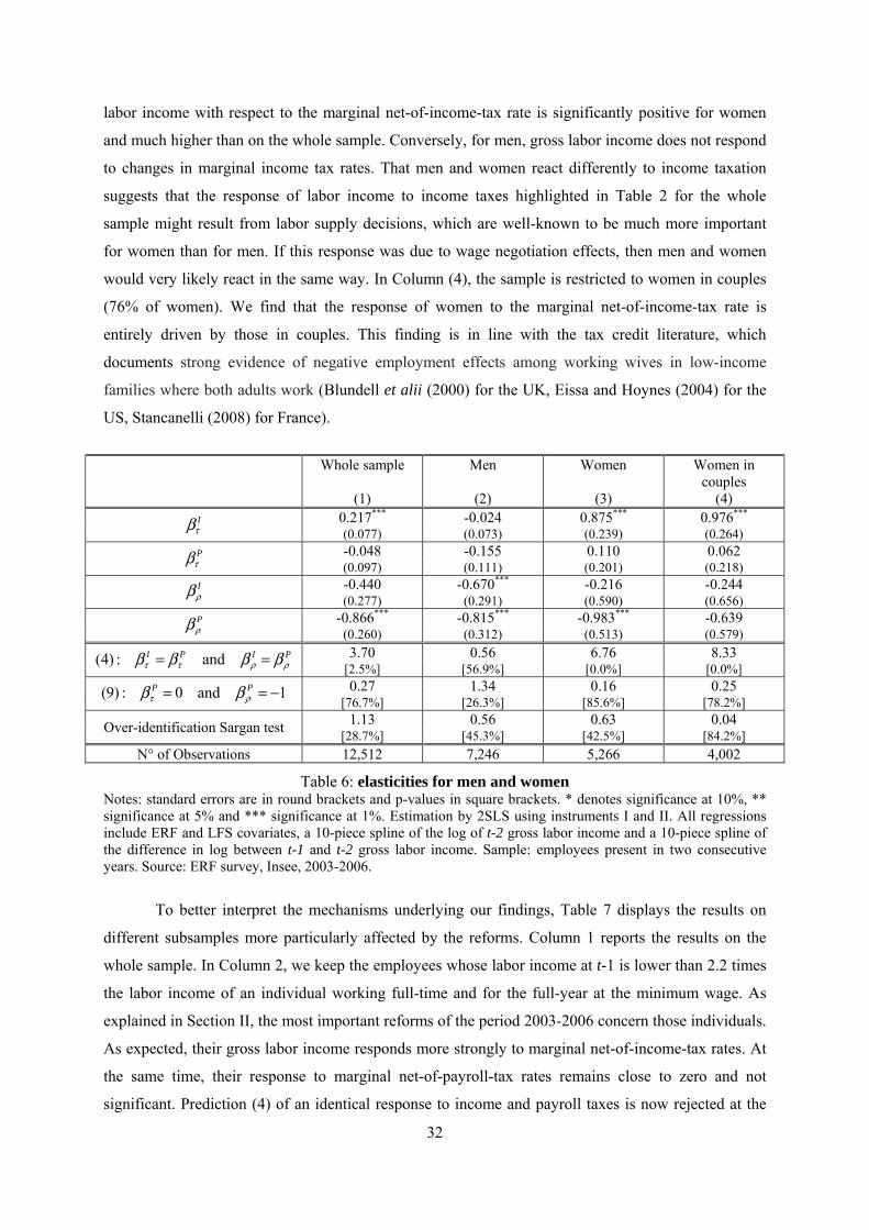
32

labor income with respect to the marginal net-of-income-tax rate is significantly positive for women

and much higher than on the whole sample. Conversely, for men, gross labor income does not respond

to changes in marginal income tax rates. That men and women react differently to income taxation

suggests that the response of labor income to income taxes highlighted in Table 2 for the whole

sample might result from labor supply decisions, which are well-known to be much more important

for women than for men. If this response was due to wage negotiation effects, then men and women

would very likely react in the same way. In Column (4), the sample is restricted to women in couples

(76% of women). We find that the response of women to the marginal net-of-income-tax rate is

entirely driven by those in couples. This finding is in line with the tax credit literature, which

documents strong evidence of negative employment effects among working wives in low-income

families where both adults work (Blundell et alii (2000) for the UK, Eissa and Hoynes (2004) for the

US, Stancanelli (2008) for France).

Whole sample

(1)

Men

(2)

Women

(3)

Women in couples

(4) I

τβ 0.217*** -0.024 0.875*** 0.976***

(0.077) (0.073) (0.239) (0.264) P

τβ -0.048 -0.155 0.110 0.062 (0.097) (0.111) (0.201) (0.218)

Iρβ -0.440 -0.670*** -0.216 -0.244

(0.277) (0.291) (0.590) (0.656) Pρβ -0.866*** -0.815*** -0.983*** -0.639

(0.260) (0.312) (0.513) (0.579)

PIPIρρττ ββββ == and:)4( 3.70 0.56 6.76 8.33

[2.5%] [56.9%] [0.0%] [0.0%]

1and0:)9( −== PPρτ ββ 0.27 1.34 0.16 0.25

[76.7%] [26.3%] [85.6%] [78.2%]

Over-identification Sargan test 1.13 0.56 0.63 0.04 [28.7%] [45.3%] [42.5%] [84.2%]

N° of Observations 12,512 7,246 5,266 4,002

Table 6: elasticities for men and women Notes: standard errors are in round brackets and p-values in square brackets. * denotes significance at 10%, ** significance at 5% and *** significance at 1%. Estimation by 2SLS using instruments I and II. All regressions include ERF and LFS covariates, a 10-piece spline of the log of t-2 gross labor income and a 10-piece spline of the difference in log between t-1 and t-2 gross labor income. Sample: employees present in two consecutive years. Source: ERF survey, Insee, 2003-2006.

To better interpret the mechanisms underlying our findings, Table 7 displays the results on

different subsamples more particularly affected by the reforms. Column 1 reports the results on the

whole sample. In Column 2, we keep the employees whose labor income at t-1 is lower than 2.2 times

the labor income of an individual working full-time and for the full-year at the minimum wage. As

explained in Section II, the most important reforms of the period 2003-2006 concern those individuals.

As expected, their gross labor income responds more strongly to marginal net-of-income-tax rates. At

the same time, their response to marginal net-of-payroll-tax rates remains close to zero and not

significant. Prediction (4) of an identical response to income and payroll taxes is now rejected at the

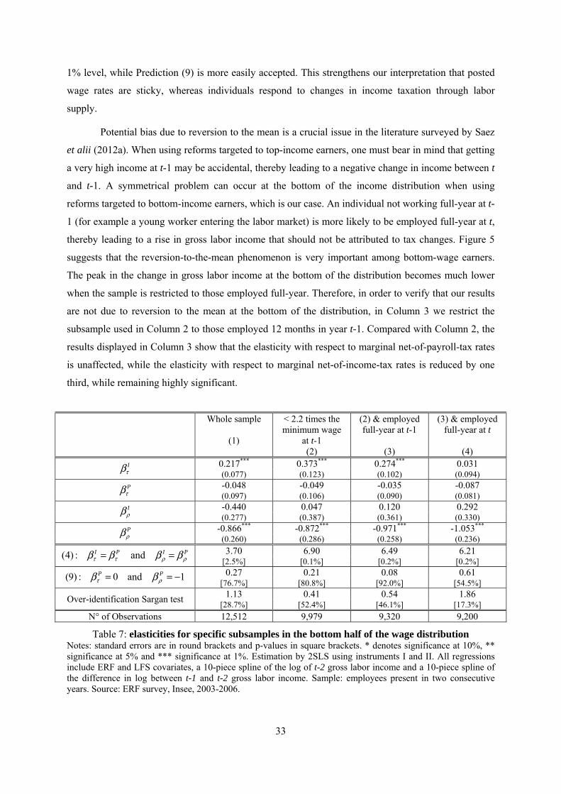
33

1% level, while Prediction (9) is more easily accepted. This strengthens our interpretation that posted

wage rates are sticky, whereas individuals respond to changes in income taxation through labor

supply.

Potential bias due to reversion to the mean is a crucial issue in the literature surveyed by Saez

et alii (2012a). When using reforms targeted to top-income earners, one must bear in mind that getting

a very high income at t-1 may be accidental, thereby leading to a negative change in income between t

and t-1. A symmetrical problem can occur at the bottom of the income distribution when using

reforms targeted to bottom-income earners, which is our case. An individual not working full-year at t-

1 (for example a young worker entering the labor market) is more likely to be employed full-year at t,

thereby leading to a rise in gross labor income that should not be attributed to tax changes. Figure 5

suggests that the reversion-to-the-mean phenomenon is very important among bottom-wage earners.

The peak in the change in gross labor income at the bottom of the distribution becomes much lower

when the sample is restricted to those employed full-year. Therefore, in order to verify that our results

are not due to reversion to the mean at the bottom of the distribution, in Column 3 we restrict the

subsample used in Column 2 to those employed 12 months in year t-1. Compared with Column 2, the

results displayed in Column 3 show that the elasticity with respect to marginal net-of-payroll-tax rates

is unaffected, while the elasticity with respect to marginal net-of-income-tax rates is reduced by one

third, while remaining highly significant.

Whole sample

(1)

< 2.2 times the minimum wage

at t-1 (2)

(2) & employed full-year at t-1

(3)

(3) & employed full-year at t

(4)

Iτβ 0.217*** 0.373*** 0.274*** 0.031

(0.077) (0.123) (0.102) (0.094) P

τβ -0.048 -0.049 -0.035 -0.087 (0.097) (0.106) (0.090) (0.081)

Iρβ -0.440 0.047 0.120 0.292

(0.277) (0.387) (0.361) (0.330) Pρβ -0.866*** -0.872*** -0.971*** -1.053***

(0.260) (0.286) (0.258) (0.236)

PIPIρρττ ββββ == and:)4( 3.70 6.90 6.49 6.21

[2.5%] [0.1%] [0.2%] [0.2%]

1and0:)9( −== PPρτ ββ 0.27 0.21 0.08 0.61

[76.7%] [80.8%] [92.0%] [54.5%]

Over-identification Sargan test 1.13 0.41 0.54 1.86 [28.7%] [52.4%] [46.1%] [17.3%]

N° of Observations 12,512 9,979 9,320 9,200

Table 7: elasticities for specific subsamples in the bottom half of the wage distribution Notes: standard errors are in round brackets and p-values in square brackets. * denotes significance at 10%, ** significance at 5% and *** significance at 1%. Estimation by 2SLS using instruments I and II. All regressions include ERF and LFS covariates, a 10-piece spline of the log of t-2 gross labor income and a 10-piece spline of the difference in log between t-1 and t-2 gross labor income. Sample: employees present in two consecutive years. Source: ERF survey, Insee, 2003-2006.

34

Employees may respond to income taxation through their choice of the number of working

months per year, i.e., an extensive or participation margin, or through hours-of-work intensive

decisions. To test for the first alternative, in Column 4, we further exclude those not employed full-

year at t, thus restricting the sample from Column 2 to those employed full-year at t and t-1. The

elasticities with respect to marginal and average net-of-payroll-tax rates are unaffected and in line with

Prediction (9) associated with posted wage rate stickiness. The novelty is that the elasticity with

respect to the marginal net-of-income-tax rate becomes very close to zero and not significant. This

suggests that the labor income responses to changes in income taxation that we find essentially reflect

participation decisions of individuals, rather than hours-of-work intensive decisions of those remaining

employed.

Conclusion

In this paper, we estimate jointly the gross labor income responses to marginal and average tax

rates for both income and payroll tax schedules. To identify the responses to the payroll tax schedule,

we use the changes in the employer payroll tax reduction for low-paid jobs that occurred in France

over the period 2003-2006. To identify the responses to the income tax schedule, we use the increase

in working tax credit for low wage earners that took place over the same period.

We find a significant elasticity of gross labor income with respect to the marginal net-of-

income-tax rate around 0.2 and our results suggest that this effect is driven by married women’s labor

supply decisions. Conversely, we find no significant effect of marginal net-of-payroll-tax rates on

gross labor income. This discrepancy appears robust across specifications and sample selections. It is

in contradiction with the prediction of identical responses to income tax and to payroll tax reforms that

is common to a large class of labor market models, in particular the competitive labor supply

framework, which is central in the optimal income taxation literature.

We also find a significant elasticity of gross labor income to the average net-of-payroll-tax

rate, which is not significantly different from minus one. Conversely, the elasticity with respect to the

average net-of-income-tax rate is much weaker and generally not significant. Among the different

theories that can account for different behavioral responses to payroll and income taxation, posted

wage rate stickiness associated with significant labor supply responses to income taxes is our preferred

interpretation.

This work can be extended in different directions. A first direction would be to consider a

longer panel of observations to investigate the long run responses to taxation. This in particular would

enable us to test whether the unresponsiveness of posted labor income to payroll taxation is only a

short run result or whether the responses of gross labor income to payroll taxation in the long run are

similar to the responses to income taxation. Another extension would be to disentangle the responses

35

we obtain in terms of wage formation, labor demand effects, participation decision effects and

intensive labor supply effects. These extensions belong to our research agenda.

References

Aeberhardt, R. and D. Sraer, 2009, Allégements de cotisations patronales et dynamique salariale, Economie et Statistique, 429-430, 177-189.

Auten, G. and R. Carroll, 1999, The Effect of Income Tax on Household Income, The Review of Economics and Statistics, 81(4), 681-93.

Avouyi-Dovi, S., D. Fougère and E. Gautier, 2011, Wage Rigidity, Collective Bargaining and the Minimum Wage: Evidence from French Agreement Data, IZA discussion paper 5835, forthcoming in Review of Economics and Statistics.

Blundell, R., A. Duncan, J. McCrae and C. Meghir, 2000, The labour market impact of the working families tax credit, Fiscal Studies, 21 (1), 65–67. http://www.ifs.org.uk/publications/fiscalstudies.

Bunel, M., F. Gilles and Y. L’Horty, 2012, The effect of social security payroll tax reductions on employment and wages: an evaluation of the 2003 French reform, forthcoming in Fiscal Studies.

Blomquist, S. and H. Selin, 2010, Hourly wage rate and taxable income responsiveness to changes in marginal tax rates, Journal of Public Economics, 94(11-12), 878-889.

Cabannes, P.-Y., Houdré, C. and Landais, C, 2011, Est-il souhaitable d'augmenter le taux supérieur d'imposition des revenus pour consolider les finances publiques ? Une estimation de l'élasticité du revenu imposable au taux marginal, mimeo.

Chetty, R., 2012, Bounds on Elasticities with Optimization Frictions: A Synthesis of Micro and Macro Evidence on Labor Supply, Econometrica, 80(3), 969-1018.

Chetty, R., A. Looney and K. Kroft, 2009, Salience and Taxation: Theory and Evidence, American Economic Review, 99(4), 1145-77.

Eissa, N. and H. Hoynes, 2004, Taxes and the labor market participation of married couples: the earned income tax credit, Journal of Public Economics, 88, 1931–1958.

Feldstein, M., 1995, The Effect of Marginal Tax Rates on Taxable Income: A Panel Study on the 1986 Tax Reform Act, Journal of Political Economy, 103(3), 551-572.

Gruber, J., 1997, The Incidence of Payroll Taxation: Evidence from Chile, Journal of Labor Economics, 15 (3, Part 2), S72-S101.

Gruber, J. and E. Saez, 2002, The elasticity of taxable income: evidence and implications, Journal of Public Economics, 84(1), 1-32.

Hersoug, T., 1984, Union Wage Responses to Tax Changes, Oxford Economic Papers, 36(1), 37-51.

Holmlund, B. and M. Söderström, 2008, Estimating Dynamic Income Responses to Tax Reforms: Swedish Evidence, Institute for Labour Market Policy Evaluation (IFAU) Working Paper 2008-28. http://www.ifau.se/Upload/pdf/se/2008/wp08-28.pdf

Kleven, H. J. and E. A. Schultz, 2012, Estimating Taxable Income Responses using Danish Tax Reforms, mimeo LSE and CBS.

Kopczuk, W., 2005, Tax bases, tax rates and the elasticity of reported income, Journal of Public Economics, 89, 2093-2119.

Kramarz, F. and T. Philippon, 2001, The impact of differential payroll tax subsidies on minimum wage employment, Journal of Public Economics, 82(1), 115–146.

Kugler, A. and M. Kugler, 2009, The Labor Market Effects of Payroll Taxes in Developing Countries: Evidence from Colombia, Economic development and cultural change, 57(2), 335-358

36

Liebman, J. and E. Saez, 2006, Earnings responses to Increases in Payroll Taxes, mimeo.

Lindsey, L., 1987, Individual taxpayer response to tax cuts: 1982-1984, with the implications for the revenue maximizing tax rate, Journal of Public Economics, 33, 173-206.

Lhommeau, B. and V. Remy, 2009, Les politiques d’allégements ont-elles un effet sur la mobilité salariale des travailleurs à bas salaires ?, Economie et Statistique, 429-430, 21-49.

Lockwood, B. and Manning A., 1993, Wage Setting and the Tax System: Theory and evidences for the United Kingdom, Journal of Public Economics, 52(1), 1-29.

Mortensen, D. and C. Pissarides, 1994, Job Creation and Job Destruction in the Theory of Unemployment, Review of Economic Studies, 61, 397-415.

Pissarides, C.A., 2000, Equilibrium Unemployment Theory, Second edition, MIT Press.

Saez, E., 2003, The effect of marginal tax rates on income: a panel study of ‘‘bracket creep’’, Journal of Public Economics, 87(5-6), 1231-1258.

Saez, E., J. Slemrod, and S. Giertz, 2012a, The Elasticity of Taxable Income with Respect to Marginal Tax Rates: A Critical Review, Journal of Economic Literature, 50(1), 3-50.

Saez, E., M. Matsaganis, and P. Tsakloglou, 2012b, Earnings determination and taxes: Evidence from a cohort based payroll tax reform in Greece, Quarterly journal of Economics, 127(1), 493-533.

Stancanelli, E., 2008, Evaluating the impact of the French Tax Credit on the employment rate of women, Journal of Public Economics, 92, 2036-47.

Weber C., 2011, Obtaining a consistent estimate of the elasticity of taxable income using difference-in-differences, mimeo, university of Michigan.

Appendix A

A.1) Derivation of Equation (3)

A compensated payroll tax reform is defined as a simultaneous change in the marginal net-of-

payroll-tax rate ΔτP and in the virtual posted income ΔRP such that the amount of payroll tax paid at

the initial gross labor income w* is kept unchanged, i.e. ΔRP = - w*ΔτP. Therefore the compensated

marginal payroll tax elasticity is defined from the “Slutsky-alike” equation:

PP

P

P

PP

PP

R

WW

wR

Ww

W

w ∂∂−

∂∂=

∂∂−

∂∂= τ

ττ

ττβτ *

** (A1)

Symmetrically, a compensated income tax reform is a simultaneous change in the marginal

net-of-income-tax rate ΔτI and in the virtual net income ΔRI such that the amount of income tax paid at

the initial gross labor income w* is kept unchanged, i.e. ΔRI = - z*ΔτI = - w* ρP ΔτI. Therefore the

compensated marginal income tax elasticity is defined as:

IPI

I

I

Ip

I

II

R

WW

wR

Ww

W

w ∂∂−

∂∂=

∂∂−

∂∂= ρτ

ττρ

ττβτ *

** (A2)

37

Combining Equations (2), (A1), (A2) leads to:

Δ+Δ∂∂+

Δ+Δ∂∂+Δ+Δ=Δ

*** w

R

R

W

w

R

R

W

w

w IIP

I

PP

PI

II

p

Pp τρτ

ττβ

ττβ ττ

Using PρΔ =ΔτP+(ΔRP/w*), IρΔ =ΔτI + ΔRI / z* - (RI/z*) PρΔ /ρP and ΔRI/w* = ρP ΔRI/z* leads to:

II

PPI

I

PI

II

p

pP

R

W

R

W

z

R

R

W

w

w ρρρττβ

ττβ ττ Δ

∂∂+Δ

∂∂+

∂∂+Δ+Δ=Δ

**

which gives Equation (3), provided that we define:

∂∂+

∂∂=

I

I

PPP

R

W

z

R

R

W*

ρβρ and I

IPI

R

W

∂∂= ρρβρ (A3)

A.2) Benchmark models: proof of Equation (4)

Differentiating both sides of Ω(τI τP,τI RP + RI) ≡ W(τI,τP,RI,RP) gives:

RR

W

RR

W

W

RR

W

IPI

IP

PPI

∂Ω∂=

∂∂

∂Ω∂=

∂∂

∂Ω∂=

∂∂

∂Ω∂+

∂Ω∂=

∂∂

τ

ττ

τττ

τ

Then, using (A1) and (A2) above leads to:

RwRw

R

wR

WW

w

RwR

WW

w

IPIP

PIP

IIP

IPI

I

II

IPIP

PP

P

PP

∂Ω∂−

∂Ω∂=

∂Ω∂

−+

∂Ω∂=

∂∂−

∂∂=

∂Ω∂−

∂Ω∂=

∂∂−

∂∂=

τττ

ττρτττ

ττρττ

τβ

τττ

ττττ

τβ

τ

τ

implying that P

τβ =I

τβ . Using (A3):

RR

W

RRz

R

R

W

z

R

R

W IPI

IPIIPI

IPI

I

PPP

∂Ω∂=

∂∂=

∂Ω∂=

∂Ω∂

+=

∂∂+

∂∂= ρρρρβρρτρρβ ρρ

38

implying that Pρβ =

Iρβ , which ends the derivation of Prediction (4). In benchmark models, the gross

labor income w maximizes ( )wRwU ,+τ in w. The first-order condition writes: F(w,τ,R)=0, where

function F(.,.,.) is defined by: ( ) ( ) ( )wRwUwRwURwF ,',',, 21 +++⋅≡ ττττ . Assuming that the

second-order condition '

wF < 0 holds with a strict inequality (which is the case if for instance U is

strictly concave), the partial derivatives of function Ω(.,.) for w*=Ω(τ,R) are:

( )'

''''

'

''and'

'''''

'

'' 12111211

*1

ww

RR

ww F

UU

F

F

F

UUwU

F

F +⋅−=−=Ω+⋅+−=−=Ω ττττ

where the partial derivatives of U are computed for w = w* and c=τw*+R. We then get:

0'

''' 1

*>

⋅

⋅−=Ω−Ω==w

RIP

Fw

U

w

τττββ τττ

where the last inequality follows 'wF < 0 and '

1U >0.

A.3) Deferred benefits leads to (6)

Assume that deferred benefits are indexed on the amount of payroll tax (1-τP)w*-RP, through

the indexation parameter k. Thus c=τP τI w + τI RP +RI + k ((1-τP)w*-RP) and the gross labor income

solves: ( )( )( )wRwkRRwU PPIPIIPw ,1max −−+++ ττττ . Let us write F(w,τP,τI,RP,RI)=0 the first-

order condition of this program, where function F(.,.,.) is now defined by:

( ) ( )( ) ( )( )( )( )PPiPIIp

PPiPIIpPIpIPiP

RkwkRRwU

RkwkRRwUkRRwF

⋅−−+++⋅⋅+

⋅−−+++⋅⋅⋅−+⋅≡

ττττ

τττττττττ

1'

1'1,,,,

2

1

Assuming that the second-order condition 'wF < 0 holds with a strict inequality (which is the case if U

is strictly concave), the partial derivatives of W(.,.,.,.) at w*=W(τP,τI,RP,RI) are:

39

( ) ( ) ( )( )

( ) ( )( )

( ) ( )( )

( )( )'

''''1

'

'

'

''''1

'

'

'

''''1'

'

'

'

''''1'

'

'

1211

1211

1211**

1

1211*

1

w

PIP

w

RI

w

PIPI

w

RP

w

PIPPPP

wI

w

PIPII

wP

F

UUk

F

F

R

W

F

UUkk

F

F

R

W

F

UUkwRwU

F

FW

F

UUkwkUk

F

FW

I

P

I

P

+−+

−=−=∂∂

+−+⋅−

−=−=∂∂

+−+⋅⋅++⋅

−=−=∂∂

+−+⋅⋅−+⋅−

−=−=∂∂

τττ

ττττ

τττττ

τ

τττττ

τ

τ

τ

Using (A1), (A2) and taking into account z*=τPw*+RP leads to the first part of (6) when 0 < k < τI.

( ) II

w

IP

PP

PP

w

IP

II

II

k

Fw

Uk

R

Ww

W

w

Fw

U

R

Wz

W

w

ττ

τ

βτ

τττ

τβ

τττ

τβ

−=⋅−⋅−=

∂∂−

∂∂=

>⋅⋅−=

∂∂−

∂∂=

1'

'

0'

'

*

1**

*

1**

where the inequalities follow the second-order conditions '

wF < 0 and '1U > 0. Applying (A3) gives:

( )( )

( )( )

( ) ( )( ) Ii

PIPI

w

P

PIPI

I

w

P

I

I

PPP

PIP

w

IP

IIPI

kUUkk

F

UUkz

Rk

FR

W

z

R

R

W

UUkFR

W

ρ

ρ

ρ

βρ

τττρρ

ττττρρβ

τττρρρρβ

−=

+−+−−=

+−+

+−−=

∂∂+

∂∂=

+−+−=

∂∂=

1''''1'

''''1'

''''1'

1211

1211**

1211

which is the second part of (6) when k < ρI.

Appendix B: additional empirical results

Table B.1 reproduces the results of the first stage equations, using the specification and

method corresponding to Column 3 of Table 2. In bold are estimates of the direct effects of jti,logτΔ

and j

ti,logτΔ on jti,logτΔ , and of

jti,log ρΔ on

jti,log ρΔ , with j=P, I:

40

Iti ,logτΔ P

ti ,logτΔ I

ti ,log ρΔ P

ti ,log ρΔ

Iti ,logτΔ 0.442*** -0.095*** -0.003** 0.001

(25.5) (-6.60) (-2.56) (0.77) P

ti ,logτΔ -0.014 0.575*** -0.002 -0.001 (-0.52) (24.20) (-0.92) (1.17)

I

ti ,logτΔ 0.029* -0.009 0.011*** -0.000 (1.93) (-0.71) (11.7) (-0.31)

I

ti ,log ρΔ 0.110 0.082 0.580*** -0.008***

(1.34) (1.20) (118.0) (-2.62) P

ti ,log ρΔ 0.096 -0.007 -0.001 0.925***

(0.78) (-0.07) (-0.17) (196.0) Tax records variables Yes Yes Yes Yes

LFS variables Yes Yes Yes Yes N° of Observations 12,512 12,512 12,512 12,512

F-Statistic 16.48*** 16.06*** 444.1*** 767.9*** Table B.1 - First-stage regressions

Notes: student statistics are in round brackets. Estimation by 2SLS using instruments I and II. Sample: employees present in two consecutive years. Source: ERF survey, Insee, 2003-2006.

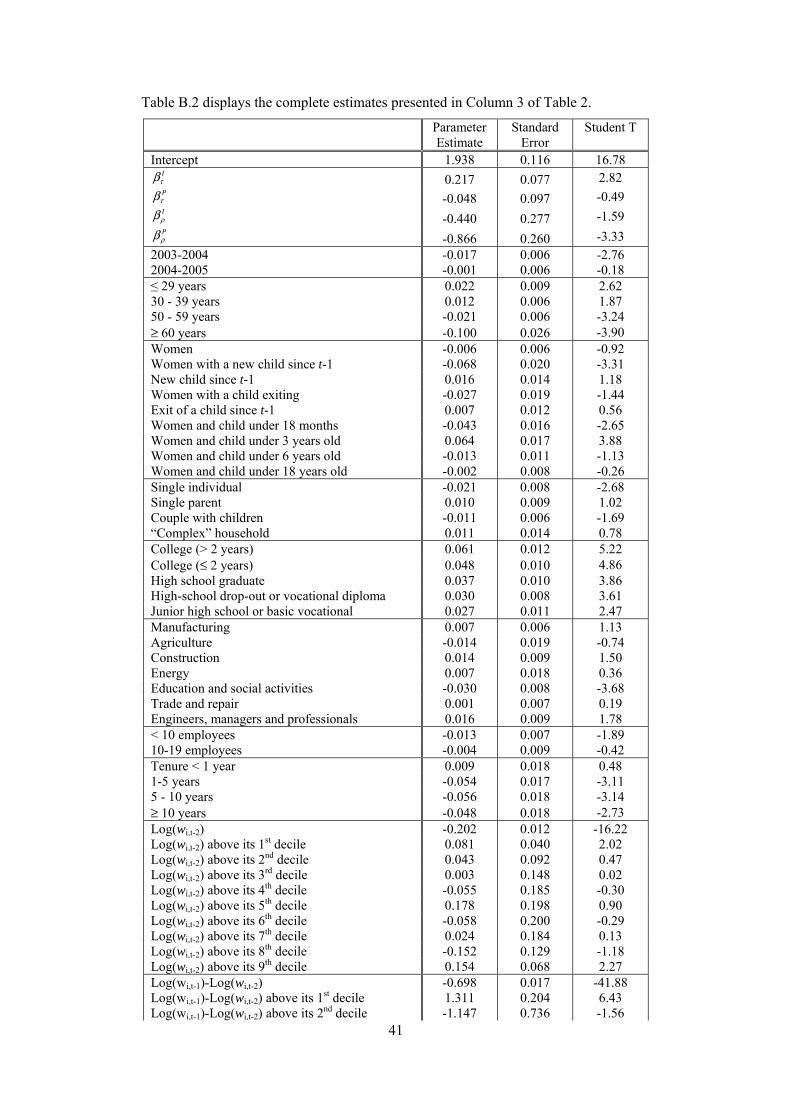
41

Table B.2 displays the complete estimates presented in Column 3 of Table 2.

Parameter Estimate

Standard Error

Student T

Intercept 1.938 0.116 16.78 I

τβ 0.217 0.077 2.82 P

τβ -0.048 0.097 -0.49 Iρβ -0.440 0.277 -1.59 Pρβ -0.866 0.260 -3.33

2003-2004 -0.017 0.006 -2.76 2004-2005 -0.001 0.006 -0.18 ≤ 29 years 0.022 0.009 2.62 30 - 39 years 0.012 0.006 1.87 50 - 59 years -0.021 0.006 -3.24 ≥ 60 years -0.100 0.026 -3.90 Women -0.006 0.006 -0.92 Women with a new child since t-1 -0.068 0.020 -3.31 New child since t-1 0.016 0.014 1.18 Women with a child exiting -0.027 0.019 -1.44 Exit of a child since t-1 0.007 0.012 0.56 Women and child under 18 months -0.043 0.016 -2.65 Women and child under 3 years old 0.064 0.017 3.88 Women and child under 6 years old -0.013 0.011 -1.13 Women and child under 18 years old -0.002 0.008 -0.26 Single individual -0.021 0.008 -2.68 Single parent 0.010 0.009 1.02 Couple with children -0.011 0.006 -1.69 “Complex” household 0.011 0.014 0.78 College (> 2 years) 0.061 0.012 5.22 College (≤ 2 years) 0.048 0.010 4.86 High school graduate 0.037 0.010 3.86 High-school drop-out or vocational diploma 0.030 0.008 3.61 Junior high school or basic vocational 0.027 0.011 2.47 Manufacturing 0.007 0.006 1.13 Agriculture -0.014 0.019 -0.74 Construction 0.014 0.009 1.50 Energy 0.007 0.018 0.36 Education and social activities -0.030 0.008 -3.68 Trade and repair 0.001 0.007 0.19 Engineers, managers and professionals 0.016 0.009 1.78 < 10 employees -0.013 0.007 -1.89 10-19 employees -0.004 0.009 -0.42 Tenure < 1 year 0.009 0.018 0.48 1-5 years -0.054 0.017 -3.11 5 - 10 years -0.056 0.018 -3.14 ≥ 10 years -0.048 0.018 -2.73 Log(wi,t-2) -0.202 0.012 -16.22 Log(wi,t-2) above its 1st decile 0.081 0.040 2.02 Log(wi,t-2) above its 2nd decile 0.043 0.092 0.47 Log(wi,t-2) above its 3rd decile 0.003 0.148 0.02 Log(wi,t-2) above its 4th decile -0.055 0.185 -0.30 Log(wi,t-2) above its 5th decile 0.178 0.198 0.90 Log(wi,t-2) above its 6th decile -0.058 0.200 -0.29 Log(wi,t-2) above its 7th decile 0.024 0.184 0.13 Log(wi,t-2) above its 8th decile -0.152 0.129 -1.18 Log(wi,t-2) above its 9th decile 0.154 0.068 2.27 Log(wi,t-1)-Log(wi,t-2) -0.698 0.017 -41.88 Log(wi,t-1)-Log(wi,t-2) above its 1st decile 1.311 0.204 6.43 Log(wi,t-1)-Log(wi,t-2) above its 2nd decile -1.147 0.736 -1.56

42

Log(wi,t-1)-Log(wi,t-2) above its 3rd decile 0.468 1.354 0.35 Log(wi,t-1)-Log(wi,t-2) above its 4th decile 0.530 1.601 0.33 Log(wi,t-1)-Log(wi,t-2) above its 5th decile -1.097 1.460 -0.75 Log(wi,t-1)-Log(wi,t-2) above its 6th decile 0.692 1.099 0.63 Log(wi,t-1)-Log(wi,t-2) above its 7th decile -0.612 0.677 -0.90 Log(wi,t-1)-Log(wi,t-2) above its 8th decile 0.522 0.312 1.67 Log(wi,t-1)-Log(wi,t-2) above its 9th decile -0.148 0.081 -1.83

Table B.2 - Full results of model (3) in Table 2 Notes: standard errors are in round brackets. Estimation by 2SLS using instruments I and II. Sample: employees present in two consecutive years. Source: ERF survey, Insee, 2003-2006.