University of Rhode Island University of Rhode Island

DigitalCommons@URI DigitalCommons@URI

Open Access Dissertations

2016

WaveQ3D: Fast and Accurate Acoustic Transmission Loss (TL) WaveQ3D: Fast and Accurate Acoustic Transmission Loss (TL)

Eigenrays, in Littoral Environments Eigenrays, in Littoral Environments

Sean M. Reilly University of Rhode Island, campreilly@my.uri.edu

Follow this and additional works at: https://digitalcommons.uri.edu/oa_diss

Recommended Citation Recommended Citation Reilly, Sean M., "WaveQ3D: Fast and Accurate Acoustic Transmission Loss (TL) Eigenrays, in Littoral Environments" (2016). Open Access Dissertations. Paper 441. https://digitalcommons.uri.edu/oa_diss/441

This Dissertation is brought to you for free and open access by DigitalCommons@URI. It has been accepted for inclusion in Open Access Dissertations by an authorized administrator of DigitalCommons@URI. For more information, please contact digitalcommons@etal.uri.edu.

WAVEQ3D: FAST AND ACCURATE ACOUSTIC TRANSMISSION LOSS (TL)

EIGENRAYS, IN LITTORAL ENVIRONMENTS

BY

SEAN M. REILLY

A DISSERTATION SUBMITTED IN PARTIAL FULFILLMENT OF THE

REQUIREMENTS FOR THE DEGREE OF DOCTOR OF PHILOSOPHY

IN OCEAN ENGINEERING

UNIVERSITY OF RHODE ISLAND

2016

DOCTOR OF PHILOSOPHY DISSERTATION

OF

SEAN M. REILLY

APPROVED:

Dissertation Committee

Major Professor Gopu R. Potty

James H. Miller

Isaac Ginis

Nasser H. Zawia

DEAN OF THE GRADUATE SCHOOL

UNIVERSITY OF RHODE ISLAND

2016

Abstract

This study defines a new 3D Gaussian ray bundling acoustic transmission loss

model in geodetic coordinates: latitude, longitude, and altitude. This approach is de-

signed to lower the computation burden of computing accurate environmental effects

in sonar training application by eliminating the need to transform the ocean environ-

ment into a collection of Nx2D Cartesian radials. This approach also improves model

accuracy by incorporating real world 3D effects, like horizontal refraction, into the

model. This study starts with derivations for a 3D variant of Gaussian ray bundles

in this coordinate system. To verify the accuracy of this approach, acoustic prop-

agation predictions of transmission loss, time of arrival, and propagation direction

are compared to analytic solutions and other models. To validate the model’s ability

to predict real world phenomena, predictions of transmission loss and propagation

direction are compared to at-sea measurements, in an environment where strong hor-

izontal refraction effect have been observed. This model has been integrated into U.S.

Navy active sonar training system applications, where testing has demonstrated its

ability to improve transmission loss calculation speed without sacrificing accuracy.

Acknowledgments

The author would like to acknowledge all of the collaborators who have assisted in

this research over the years. In 1994, Dr. Roy Deavenport (Naval Undersea Warfare

Center Division Newport) first encouraged me to explore the development of a 3D

Gaussian beam theory to support the modeling of the environmental impulse response

for active sonar applications. The theory for reflection from a 3-D slope was developed

by Dr. Michael Goodrich (Alion Science and Technology), who also made significant

contributions to the development of test cases as part of an internal research and

development effort funded by Alion Science and Technology in 2009. Efforts to test

and productize this model where funded from 2011-2015 by the High Frequency Ac-

tive Sonar Training (HiFAST) project at the U.S. Office of Naval Research (ONR),

where Mr. Michael Vaccaro led the charge to evolve this unproven concept into a

Navy training capability. Mr. David Thibaudeau provided testing support and Mr.

Ted Burns acted as our the lead system integrator during the HiFAST effort at Aegis

Technology Group. Thanks to Dr. Thomas Yudichak (Applied Research Laboratory

at the University of Texas in Austin), who provided years of Navy certification expe-

rience and keen insights during the his independent verification and validation effort.

Special thanks are due to Jonathan Glass, and his team at Naval Air Warfare Center

Training System Division, who suffered through the first integration of the this model

into a real Navy training system. Finally, the author would like to thank Dr. Gopu

iii

Potty and Dr. James Miller who brought their academic rigor and perspective to this

effort.

iv

Dedication

To my wife, Joan, my inspiration in all things.

v

Preface

Many underwater acoustic propagation models transform the three dimensional (3D)

environment into a collection of two dimensional (2D) radials, and then compute

transmission loss as a function of range and depth along each of those radials. This

approach, often called Nx2D, is used in tactical decision aids to compute millions of

range, depth, and bearing combinations in just a few minutes. Sonar training ap-

plications have an additional requirement that the results must be computed in real

time for presentation to the trainees. In littoral environments, the number of acoustic

contacts can be in the hundreds, and the Nx2D approach places a large computation

burden on the training system. The primary goal of this research is to develop a

transmission loss model that reduces the computational burden on training systems

without sacrificing accuracy. Improving the speed of this computation reduce acqui-

sition costs by reducing reliance on massively parallel computing systems. This study

also seeks to provide the acoustics research community with a tool that can predict 3D

effects in applications, like geophysical parameter inversion, where execution speed is

important.

This dissertation follows the University of Rhode Island Graduate School guide-

lines for the preparation of a dissertation in manuscript format. There are three

chapters that represent formally published papers:

• Manuscript 1 derives the theory behind the model, and provides key test results

vi

including: ray path refraction accuracy using a Munk profile, Gaussian beam

projection into the shadow zone for an n2 linear profile, and horizontal refraction

from a 3D analytic wedge.

• Manuscript 2 compares model predictions to at-sea measurements of horizontal

refraction in a sloped environment.

• Manuscript 3 discusses the application of this model in deployable sonar training

systems.

• Manuscript 4 discusses the accuracy of this model in the deep sound channel.

Appendix A is an unpublished model accuracy test report, delivered to the High Fre-

quency Active Sonar Training (HiFAST) project at the U.S. Office of Naval Research

(ONR), in 2012.

vii

Table of Contents

Abstract . . . . . . . . . . . . . . . . . . . . . . . . . . . . . . . . . . . . . . ii

Acknowledgments . . . . . . . . . . . . . . . . . . . . . . . . . . . . . . . . . iii

Preface . . . . . . . . . . . . . . . . . . . . . . . . . . . . . . . . . . . . . . . vi

Table of Cotents . . . . . . . . . . . . . . . . . . . . . . . . . . . . . . . . . . viii

List of Figures . . . . . . . . . . . . . . . . . . . . . . . . . . . . . . . . . . . xii

List of Tables . . . . . . . . . . . . . . . . . . . . . . . . . . . . . . . . . . . xvii

1 Computing Acoustic Transmission Loss Using 3D Gaussian Ray

Bundles in Geodetic Coordinates . . . . . . . . . . . . . . . . . . . . . . 1

1.1 Abstract . . . . . . . . . . . . . . . . . . . . . . . . . . . . . . . . . . 2

1.2 Introduction . . . . . . . . . . . . . . . . . . . . . . . . . . . . . . . . 2

1.3 Derivation . . . . . . . . . . . . . . . . . . . . . . . . . . . . . . . . . 4

1.3.1 3-D ray propagation in spherical coordinates . . . . . . . . . . 5

1.3.2 3-D interface reflections . . . . . . . . . . . . . . . . . . . . . . 11

1.3.3 3-D eigenray path detection . . . . . . . . . . . . . . . . . . . . 15

1.3.4 3-D Gaussian ray bundles . . . . . . . . . . . . . . . . . . . . . 19

viii

1.4 Test Results . . . . . . . . . . . . . . . . . . . . . . . . . . . . . . . . 22

1.4.1 Refraction accuracy benchmark . . . . . . . . . . . . . . . . . . 22

1.4.2 2-D transmission loss benchmark . . . . . . . . . . . . . . . . . 25

1.4.3 3-D transmission loss benchmark . . . . . . . . . . . . . . . . . 28

1.4.4 Computational efficiency . . . . . . . . . . . . . . . . . . . . . 32

1.5 Conclusions . . . . . . . . . . . . . . . . . . . . . . . . . . . . . . . . 35

1.6 Acknowledgments . . . . . . . . . . . . . . . . . . . . . . . . . . . . . 36

2 Investigation of horizontal refraction on Florida Straits continental

shelf using a three-dimensional Gaussian ray bundling model . . . . . . 37

2.1 Abstract . . . . . . . . . . . . . . . . . . . . . . . . . . . . . . . . . . 38

2.2 Introduction . . . . . . . . . . . . . . . . . . . . . . . . . . . . . . . . 38

2.3 Experiment . . . . . . . . . . . . . . . . . . . . . . . . . . . . . . . . . 39

2.4 Comparison of measurements with model predictions . . . . . . . . . 42

2.5 Acknowledgments . . . . . . . . . . . . . . . . . . . . . . . . . . . . . 46

3 How the U.S Navy is Migrating from Legacy/Large Footprint to Low

Cost/Small Footprint Sonar Simulation Systems . . . . . . . . . . . . . 48

3.1 Abstract . . . . . . . . . . . . . . . . . . . . . . . . . . . . . . . . . . 49

3.2 Introduction . . . . . . . . . . . . . . . . . . . . . . . . . . . . . . . . 50

3.3 Wavefront Queue 3-D Model . . . . . . . . . . . . . . . . . . . . . . . 53

3.4 Speed and Accuracy Testing . . . . . . . . . . . . . . . . . . . . . . . 57

3.5 Integration into Training System . . . . . . . . . . . . . . . . . . . . . 60

3.6 Conclusions . . . . . . . . . . . . . . . . . . . . . . . . . . . . . . . . 64

ix

3.7 Acknowledgments . . . . . . . . . . . . . . . . . . . . . . . . . . . . . 65

3.8 About the Authors . . . . . . . . . . . . . . . . . . . . . . . . . . . . 65

4 Evaluating accuracy limits of Gaussian ray bundling model in the deep

sound channel . . . . . . . . . . . . . . . . . . . . . . . . . . . . . . . . . 67

4.1 Abstract . . . . . . . . . . . . . . . . . . . . . . . . . . . . . . . . . . 68

4.2 Introduction . . . . . . . . . . . . . . . . . . . . . . . . . . . . . . . . 68

4.3 Benchmark solution for Snell’s Law in spherical media . . . . . . . . . 69

4.4 Equivalent benchmark solution in Cartesian coordinates . . . . . . . . 73

4.5 WaveQ3D accuracy . . . . . . . . . . . . . . . . . . . . . . . . . . . . 78

4.6 Conclusions . . . . . . . . . . . . . . . . . . . . . . . . . . . . . . . . 80

A Verification Tests for Hybrid Gaussian Beams in Spherical/Time

Coordinates . . . . . . . . . . . . . . . . . . . . . . . . . . . . . . . . . . . 82

A.1 Abstract . . . . . . . . . . . . . . . . . . . . . . . . . . . . . . . . . . 83

A.2 Introduction . . . . . . . . . . . . . . . . . . . . . . . . . . . . . . . . 83

A.3 Ray Tracing Tests . . . . . . . . . . . . . . . . . . . . . . . . . . . . . 84

A.3.1 Comparisons to “flat earth” benchmarks . . . . . . . . . . . . . 85

A.3.2 Ray path accuracy in a deep sound channel . . . . . . . . . . . 90

A.3.3 Ray path accuracy in an extreme downward refraction

environment . . . . . . . . . . . . . . . . . . . . . . . . . . . 92

A.3.4 Ray path accuracy along great circle routes . . . . . . . . . . . 94

A.4 Interface Reflection Tests . . . . . . . . . . . . . . . . . . . . . . . . . 97

A.4.1 Reflection accuracy with a flat bottom . . . . . . . . . . . . . . 98

x

A.4.2 Reflection accuracy with a sloped bottom . . . . . . . . . . . . 100

A.4.3 Out-of-plane reflection from gridded bathymetry . . . . . . . . 101

A.5 Eigenray and Propagation Loss Tests . . . . . . . . . . . . . . . . . . 103

A.5.1 Eigenray accuracy for a simple geometry . . . . . . . . . . . . . 106

A.5.2 Eigenray accuracy for Lloyd’s mirror on spherical earth . . . . 108

A.5.3 Eigenray robustness for Lloyd’s mirror on spherical earth . . . 113

A.5.4 Propagation loss accuracy for Lloyd’s Mirror . . . . . . . . . . 116

A.5.5 Eigneray and propagation loss accuracy in an extreme

downward refraction environment . . . . . . . . . . . . . . . . 120

A.6 Derivations . . . . . . . . . . . . . . . . . . . . . . . . . . . . . . . . . 132

A.6.1 Ray path derivation for concave ocean surface . . . . . . . . . 132

A.6.2 Tangent spaced depression/elevation angles . . . . . . . . . . . 134

A.6.3 Propagation loss error statistics . . . . . . . . . . . . . . . . . . 136

A.7 Summary . . . . . . . . . . . . . . . . . . . . . . . . . . . . . . . . . . 137

A.8 Acknowledgments . . . . . . . . . . . . . . . . . . . . . . . . . . . . . 138

Bibliography . . . . . . . . . . . . . . . . . . . . . . . . . . . . . . . . . . . . 139

xi

List of Figures

1.1 Acoustic rays are a vector field normal to the wavefront at each point

in space. . . . . . . . . . . . . . . . . . . . . . . . . . . . . . . . . 5

1.2 Reflection from 3-D bathymetry causes ray paths to bend in the

horizontal direction. . . . . . . . . . . . . . . . . . . . . . . . . . . 12

1.3 Geometry for estimating time of impact and reflection direction from

a 3-D slope. . . . . . . . . . . . . . . . . . . . . . . . . . . . . . . . . 13

1.4 3-D refraction around a seamount (top down view, 50 m contours). 15

1.5 3-D refraction around a seamount (side view, 50 m contours). . . . 16

1.6 Eigenray estimation geometry (side view: ϕk direction not shown). . 17

1.7 Gaussian ray nearest neighbors (front view: tn direction not shown). 20

1.8 Munk profile (left panel) and modeled ray paths (right panel). . . . 24

1.9 Cycle range difference between model and analytic solution for Munk

profile ray traces. . . . . . . . . . . . . . . . . . . . . . . . . . . . . 26

1.10 Pederson profile (left panel) and modeled ray paths (right panel). . 27

1.11 Gaussian beam projection into the shadow zone for an n2 linear

profile at 2000 Hz. . . . . . . . . . . . . . . . . . . . . . . . . . . . 28

1.12 Geometry for method of images in a 3-D wedge. . . . . . . . . . . . 29

xii

1.13 Incoherent transmission loss at 2000 Hz for 3-D wedge and flat

bottom. . . . . . . . . . . . . . . . . . . . . . . . . . . . . . . . . . 33

1.14 Comparison to CASS/GRAB executions times as a function of

number of targets. . . . . . . . . . . . . . . . . . . . . . . . . . . . 34

2.1 (a) Area of operations showing source track (white dotted line). The

sand-limestone boundary from Ballard4 is shown as black continuous

line. The black dashed line is the modified boundary proposed by

this study. (b) average sound velocity profiles along 350 m, 250 m,

and 130 m contours (c) bottom loss for sand and limestone. . . . . 40

2.2 Compare modeled horizontal refraction to measured data. . . . . . 44

2.3 Modeled horizontal refraction with thin sediment layers. . . . . . . 45

3.1 Fleet Synthetic Training Concept . . . . . . . . . . . . . . . . . . . 52

3.2 Mission Rehearsal Tactical Team Trainer (MRT3) . . . . . . . . . . 53

3.3 Extract 2-D radial and compute transmission loss . . . . . . . . . . 55

3.4 Caching data in latitude, longitude, and depth coordinates . . . . . 56

3.5 Execution speed comparison . . . . . . . . . . . . . . . . . . . . . . 58

3.6 Accuracy comparison . . . . . . . . . . . . . . . . . . . . . . . . . . 60

3.7 AP module Processing . . . . . . . . . . . . . . . . . . . . . . . . . 61

3.8 Comparison of sonar displays on BATTT . . . . . . . . . . . . . . . 63

xiii

4.1 (a) Munk profile, an idealized representation of deep sound channel

conditions in the North Pacific. (left panel) Ray paths trapped in the

deep sound channel. . . . . . . . . . . . . . . . . . . . . . . . . . . . 70

4.2 (a) Munk profile (b) eigenrays to a target at 200 km, computing

using Snell’s Law for spherical media, legend indicates launch angle. 71

4.3 Range difference between Cartesian and spherical benchmark

solutions to Snell’s Law, using difference versions of the Earth

Flattening Transform. . . . . . . . . . . . . . . . . . . . . . . . . . . 76

4.4 Travel time difference between Cartesian and spherical benchmark

solutions to Snell’s Law, using difference versions of the Earth

Flattening Transform. . . . . . . . . . . . . . . . . . . . . . . . . . . 77

4.5 Range difference between WaveQ3D and Snell’s Law in spherical

media, for 25 ms time step, after 4 complete cycles. Includes

comparison to Flat Earth Transform with no approximations. . . . . 78

4.6 Travel time difference between WaveQ3D and Snell’s Law in

spherical media, for 25 ms time step. Includes comparison to Flat

Earth Transform with no approximations. . . . . . . . . . . . . . . . 79

A.1 Modeled ray paths for the Munk profile. . . . . . . . . . . . . . . . 87

A.2 earth-flattening accuracy for the Munk profile. . . . . . . . . . . . 89

A.3 WaveQ3D errors for the Munk profile. . . . . . . . . . . . . . . . . 91

A.4 Path accuracy sensitivity to step size for the Munk profile. . . . . . 92

A.5 Modeled ray paths for the Pedersen/Gordon profile. . . . . . . . . 93

xiv

A.6 Path accuracy sensitivity to step size for the Pedersen/Gordon profile. 95

A.7 Ray path accuracy as a function of step size for the

Pedersen/Gordon profile. . . . . . . . . . . . . . . . . . . . . . . . 96

A.8 Great circle routes. . . . . . . . . . . . . . . . . . . . . . . . . . . . 97

A.9 Flat bottom reflection geometry. . . . . . . . . . . . . . . . . . . . 99

A.10 Flat bottom reflection test results. . . . . . . . . . . . . . . . . . . 101

A.11 Analytic slope reflection test results. . . . . . . . . . . . . . . . . . 102

A.12 Reflection on the Malta Escarpment. . . . . . . . . . . . . . . . . . 103

A.13 Flat bottom eigenray test geometry. . . . . . . . . . . . . . . . . . 106

A.14 Isovelocity paths in spherical coordinates. . . . . . . . . . . . . . . 109

A.15 Isovelocity paths in Cartesian coordinates. . . . . . . . . . . . . . . 110

A.16 Ocean surface as concave reflector. . . . . . . . . . . . . . . . . . . 111

A.17 Roots of surface reflection transcendental equation. . . . . . . . . . 112

A.18 Eigenray errors for Lloyd’s mirror direct path. . . . . . . . . . . . . 114

A.19 Eigenray errors for Lloyd’s mirror surface reflected path. . . . . . . 116

A.20 Time-step effects near the ocean surface. . . . . . . . . . . . . . . . 117

A.21 Lloyd’s mirror propagation loss as a function of range. . . . . . . . 118

A.22 Lloyd’s mirror propagation loss errors at short ranges. . . . . . . . 119

A.23 Lloyd’s mirror propagation loss as a function of depth. . . . . . . . 120

A.24 Ray trace for shallow source. . . . . . . . . . . . . . . . . . . . . . 122

A.25 Direct path eigenrays for shallow source. . . . . . . . . . . . . . . . 123

A.26 Surface reflected eigenrays for shallow source. . . . . . . . . . . . . 124

A.27 Propagation loss for shallow source. . . . . . . . . . . . . . . . . . 126

xv

A.28 Ray trace for shallow source. . . . . . . . . . . . . . . . . . . . . . 128

A.29 Caustic eigenrays for deep source. . . . . . . . . . . . . . . . . . . 129

A.30 Direct path eigenrays for deep source. . . . . . . . . . . . . . . . . 130

A.31 Propagation loss for deep source. . . . . . . . . . . . . . . . . . . . 131

A.32 Tangent spaced beams. . . . . . . . . . . . . . . . . . . . . . . . . 134

xvi

List of Tables

3.1 Differences in WaveQ3D eigenrays, relative to FeyRay. . . . . . . . . . 64

4.1 Eigenrays to a target at 200 km, computing using Snell’s Law in

spherical media. . . . . . . . . . . . . . . . . . . . . . . . . . . . . . . 72

4.2 Largest errors for each versions of the Earth Flattening Transform. . 75

4.3 Largest errors for each step size in WaveQ3D . . . . . . . . . . . . . . 79

A.1 Flat bottom expected values. . . . . . . . . . . . . . . . . . . . . . . . 100

A.2 Expected eigenray values for a simple geometry. . . . . . . . . . . . . 108

A.3 Expected eigenray values for target at 1.2o and 150 m. . . . . . . . . . 113

A.4 Lloyd’s Mirror propagation loss accuracy. . . . . . . . . . . . . . . . . 121

A.5 Individual eigenrays for shallow source. . . . . . . . . . . . . . . . . . 125

A.6 Total propagation loss for shallow source. . . . . . . . . . . . . . . . . 127

A.7 Individual eigenrays for deep source. . . . . . . . . . . . . . . . . . . . 131

A.8 Total propagation loss for deep source. . . . . . . . . . . . . . . . . . . 132

xvii

Manuscript 1

Computing Acoustic Transmission Loss Using 3D Gaussian Ray Bundles in

Geodetic Coordinates

by

Sean M. Reilly and Gopu R. Potty

Ocean Engineering Department, University of Rhode Island

Narragansett, Rhode Island 02882

Michael Goodrich

Alion Science and Technology Corporation

Norfolk, Virginia 02882

Published in the Journal of Computational Acoustics, March 2016

1

1.1 Abstract

This paper defines a new 3-D Gaussian ray bundling model in geodetic coordinates:

latitude, longitude, and altitude. Derivations are provided for 3-D refraction, 3-

D interface reflection, 3-D eigenray detection, and a 3-D variant of CASS/GRAB

Gaussian ray bundles. This approach allows environmental parameters and their

derivatives are computed directly in latitude, longitude, and depth directions without

reducing the problem to a series of Nx2-D Cartesian projections. Our model supports

3-D effects such as great circle routes and horizontal refraction in sloped environments.

Key test results are included for ray path refraction accuracy using a Munk profile,

Gaussian beam projection into the shadow zone for an n2 linear profile, and horizontal

refraction from a 3-D analytic wedge. Testing to date indicates that this approach

has accuracy at least as good as CASS/GRAB, but with improved execution speed

benefits for large numbers of targets, and 3-D transmission loss effects.

1.2 Introduction

Many underwater acoustic propagation models transform the three dimensional (3-

D) environment into a collection of two dimensional (2-D) radials, and then compute

transmission loss as a function of range and depth along each of those radials. This

approach, often called Nx2-D, is used in tactical decision aids to compute millions

of range, depth, and bearing combinations in just a few minutes. Sonar training

applications have an additional requirement that the results must be computed in

2

real time for presentation to the trainees. In littoral environments, the number of

acoustic contacts can be in the hundreds, and transmission loss calculations place a

large computation burden on the training system. The primary goal of this research

is to develop a transmission loss model that reduces the computational burden on

training systems without sacrificing accuracy. Research into improving the speed

of this computation may reduce acquisition costs by reducing reliance on massively

parallel computing systems. The High Fidelity Active Sonar Training (HiFAST)

Project at the U.S. Office of Naval Research funded this research to provide fast

and accurate acoustic transmission loss predictions for hardware-in-the loop (HWIL)

active sonar training applications.

There are several ongoing efforts to deliver 3-D versions of Parabolic Equation25;24

and Normal Mode4 models. However, these models require large numbers of modes at

frequencies above 1000 Hz, and this impedes their ability to provide real-time, active

sonar results on low cost computer hardware. This paper develops a new acoustic

transmission loss model using 3-D ray theory in geodetic coordinates. Unlike other

efforts to model ray theory in geodetic coordinates,23 our model focuses on localized

propagation in littoral environments, instead of propagation on a global scale. This

difference requires our model to support not only 3-D refraction by the speed of

sound, but also geodetic implementations of interface reflection, eigenray detection,

and transmission loss computation.

Databases of 3-D environmental parameters are usually provided in geodetic co-

ordinates: latitude, longitude, and altitude (or depth). Instead of transforming the

3-D environment into a collection of Nx2-D radials, we maintain the 3-D nature of

3

the environment by using spherical polar coordinates (r,θ,φ) to solve the acoustic

eikonal equation. The impulse response of the environment is modeled as a series of

acoustic wavefronts that propagate away from the source as a function of time. To im-

prove transmission loss accuracy in neighborhood of shadow zones and caustics, this

derivation includes the development of a 3-D variant of the Gaussian Ray Bundling

(GRAB) model.45;17 Each wavefront has the ability to compute transmission loss to

large numbers of acoustic contacts and share the overhead of the wavefront propa-

gation computation across those contacts. Eigenrays are computed in reaction to a

collision of the wavefront with acoustic contacts.

Section 2 of this paper develops the underlying equations used to implement our

model. Section 3 provides some of the key testing results used to verify model accu-

racy. Even though this model was developed with the primary objective of supporting

the sonar training applications, the model inherently 3-D in nature and supports the

physics of out-of-plane propagation effects. Hence, this model could be a useful tool

to explore 3-D propagation effects in other research studies.41;18;3

1.3 Derivation

This section develops an implementation of 3-D refraction in spherical coordinates,

interface reflection in this coordinate system, eigenray detection, and Gaussian ray

bundle transmission loss.

4

Figure 1.1: Acoustic rays are a vector field normal to the wavefront at each point inspace.

1.3.1 3-D ray propagation in spherical coordinates

Ray theory is a high frequency approximation of the wave equation that decomposes

the acoustic impulse response of the environment into surfaces of constant travel time

(t) from the source (Fig. 1.1). The rays are a vector field ~r that is normal to these

surfaces at each point in space, and the path of these rays through the medium defines

the direction of propagation. The fundamental equations of ray theory are derived

by seeking power series solutions21 to the Helmholtz equation.

∇2p(~r) +ω2

c2(~r)p(~r) = −δ(~r − ~r0) (1.1)

p(~r) = eiωt(~r)∞∑j=0

Aj(~r)

(iω)j(1.2)

where p(~r) is the acoustic pressure as a function of location, ~r0 is the source position,

c(~r) is the speed of sound in water, t(~r) is the travel time, ω is the angular frequency,

and Aj(~r) are the components of acoustic amplitude. Equating terms of like order in

5

ω yields an infinite sequence of equations.

O(ω2) :∣∣∣~∇t∣∣∣2 =

1

c2(~r)(1.3)

O(ω) : 2~∇A0 · ~∇t+ (∇2t)A0 = 0 (1.4)

O(ω1−j) : 2~∇Aj · ~∇t+ (∇2t)Aj = −∇2Aj−1 for j=1,2,... (1.5)

The eikonal equation (1.3) defines the relationship between the direction of propa-

gation and the speed of sound in water. The first transport equation (1.4) relates the

spreading loss of the acoustic field to divergence in the propagation direction. The

remaining transport equations (1.5) relate the spreading loss of the acoustic field to

diffraction effects. Eqs. (1.3) and (1.4) are an exact solution of the wave equation

in the geometric limit, that is, when the sound speed gradient along the direction of

motion changes slowly compared to the acoustic wavelength. This accuracy breaks

down at lower frequencies where diffraction becomes a significant feature of acoustic

propagation.

Eq. (1.3) can be solved by recognizing that the direction of propagation is related

to the gradient of the travel time.

n =d~r

ds= c~∇t (1.6)

where n is the direction of propagation and s is the distance along the ray path.

Applying Eq. (1.6) to Eq. (1.3) yields a second order ordinary differential equation

in terms of ~r, c, and s.

d

ds

(1

c

d~r

ds

)= − 1

c2~∇c (1.7)

6

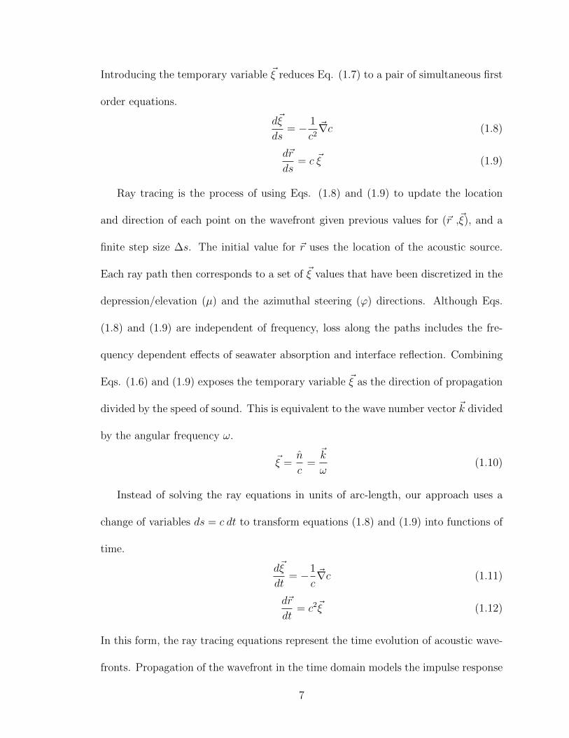
Introducing the temporary variable ~ξ reduces Eq. (1.7) to a pair of simultaneous first

order equations.

d~ξ

ds= − 1

c2~∇c (1.8)

d~r

ds= c ~ξ (1.9)

Ray tracing is the process of using Eqs. (1.8) and (1.9) to update the location

and direction of each point on the wavefront given previous values for (~r ,~ξ), and a

finite step size ∆s. The initial value for ~r uses the location of the acoustic source.

Each ray path then corresponds to a set of ~ξ values that have been discretized in the

depression/elevation (µ) and the azimuthal steering (ϕ) directions. Although Eqs.

(1.8) and (1.9) are independent of frequency, loss along the paths includes the fre-

quency dependent effects of seawater absorption and interface reflection. Combining

Eqs. (1.6) and (1.9) exposes the temporary variable ~ξ as the direction of propagation

divided by the speed of sound. This is equivalent to the wave number vector ~k divided

by the angular frequency ω.

~ξ =n

c=~k

ω(1.10)

Instead of solving the ray equations in units of arc-length, our approach uses a

change of variables ds = c dt to transform equations (1.8) and (1.9) into functions of

time.

d~ξ

dt= −1

c~∇c (1.11)

d~r

dt= c2~ξ (1.12)

In this form, the ray tracing equations represent the time evolution of acoustic wave-

fronts. Propagation of the wavefront in the time domain models the impulse response

7

of the environment, which is a useful form for broadband modeling.

Converting Eqs. (1.11) and (1.12) into spherical coordinates require a representa-

tion of d~ξ/dt and d~r/dt in that coordinate system. This derivation uses arrows for

vectors with magnitude and direction (such as ~r), carets for unit length vectors (such

as r), and plain text for magnitude parameters (such as r). The vector form of the

time derivatives is found by recognizing that ~r only has radial components, while ~ξ

has components in all three dimensions

~r(t) = r(t)r(t) (1.13)

~ξ(t) = α(t)r(t) + β(t)θ(t) + γ(t)φ(t) (1.14)

d~r

dt=dr

dtr + r

dr

dt(1.15)

d~ξ

dt=dα

dtr + α

dr

dt+dβ

dtθ + β

dθ

dt+dγ

dtφ+ γ

dφ

dt(1.16)

where α(t), β(t), and γ(t) are the r, θ, and φ components of ~ξ . The time derivatives

of r, θ, and φ are computed using a conversion into Cartesian coordinates.

r(t) = sinθ(t) cosφ(t) i+ sinθ(t) sinφ(t) j + cosθ(t) k (1.17)

θ(t) = cosθ(t) cosφ(t) i+ cosθ(t) sinφ(t) j − sinθ(t) k (1.18)

φ(t) = −sinφ(t) i+ cosφ(t) j (1.19)

The chain rule, when applied to Eqs. (1.17), (1.18), and (1.19), yields the time deriva-

tives in spherical coordinates.

dr

dt=dθ

dtθ + sinθ

dφ

dtφ (1.20)

dθ

dt= −dθ

dtr + cosθ

dφ

dtφ (1.21)

8

dφ

dt= −sinθdφ

dtr (1.22)

Applying Eqs. (1.20) through (1.22) to Eqs. (1.15) and (1.16) transforms Eqs. (1.11)

and (1.12) into spherical coordinates.

d~r

dt=dr

dtr + r

dθ

dtθ + rsinθ

dφ

dtφ (1.23)

d~ξ

dt=

[dα

dt− βdθ

dt+ γsinθ

dφ

dt

]r +

[dβ

dt+ α

dθ

dt− γcosθdφ

dt

]θ

+

[dγ

dt+ (αsinθ + βcosθ)

dφ

dt

]φ

(1.24)

Matching terms for r, θ, and φ yields a system of six scalar first-order differential

equations.

dr

dt= c2α (1.25)

rdθ

dt= c2β (1.26)

rsinθdφ

dt= c2γ (1.27)

dα

dt− βdθ

dt− γsinθdφ

dt= −1

c

dc

dr(1.28)

dβ

dt+ α

dθ

dt− γcosθdφ

dt= − 1

cr

dc

dθ(1.29)

dγ

dt+ (αsinθ + βcosθ)

dφ

dt= − 1

crsinθ

dc

dφ(1.30)

When Eqs. (1.25) though (1.27) are combined with Eqs. (1.28) though (1.30), the

system is reduced to a state where all of the coordinate derivatives appear only once.

dr

dt= c2α (1.31)

dθ

dt=c2β

r(1.32)

dφ

dt=

c2γ

rsinθ(1.33)

9

dα

dt= −1

c

dc

dr+c2

r

(β2 + γ2

)(1.34)

dβ

dt= − 1

cr

dc

dθ− c2

r

(αβ + γ2cotθ

)(1.35)

dγ

dt= − 1

crsinθ

dc

dφ− c2γ

r(α + βcotθ) (1.36)

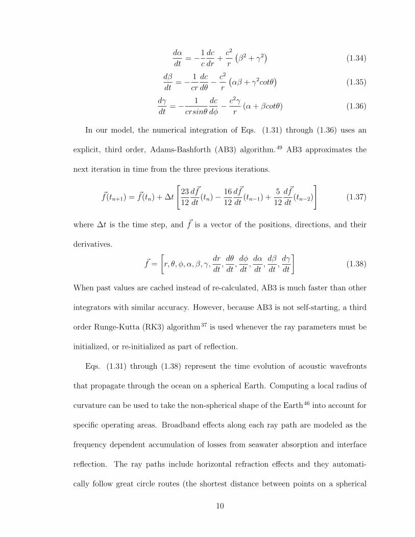
In our model, the numerical integration of Eqs. (1.31) through (1.36) uses an

explicit, third order, Adams-Bashforth (AB3) algorithm.49 AB3 approximates the

next iteration in time from the three previous iterations.

~f(tn+1) = ~f(tn) + ∆t

[23

12

d~f

dt(tn)− 16

12

d~f

dt(tn−1) +

5

12

d~f

dt(tn−2)

](1.37)

where ∆t is the time step, and ~f is a vector of the positions, directions, and their

derivatives.

~f =

[r, θ, φ, α, β, γ,

dr

dt,dθ

dt,dφ

dt,dα

dt,dβ

dt,dγ

dt

](1.38)

When past values are cached instead of re-calculated, AB3 is much faster than other

integrators with similar accuracy. However, because AB3 is not self-starting, a third

order Runge-Kutta (RK3) algorithm37 is used whenever the ray parameters must be

initialized, or re-initialized as part of reflection.

Eqs. (1.31) through (1.38) represent the time evolution of acoustic wavefronts

that propagate through the ocean on a spherical Earth. Computing a local radius of

curvature can be used to take the non-spherical shape of the Earth46 into account for

specific operating areas. Broadband effects along each ray path are modeled as the

frequency dependent accumulation of losses from seawater absorption and interface

reflection. The ray paths include horizontal refraction effects and they automati-

cally follow great circle routes (the shortest distance between points on a spherical

10

Earth) as they traverse latitudes and longitudes. Environmental parameters and their

derivatives are computed directly in the latitude, longitude, and depth directions.

This approach was selected to avoid the computation burden of converting 3-D

environmental data into Nx2-D radials. However, this choice comes at the price of

propagation equations that are much more complex than their Cartesian equivalents.

Counterintuitively, the inclusion of spherical coordinate terms in Eqs. (1.31) through

(1.36) has little impact on computational speed when the application relies on inter-

polations of gridded environmental data. On modern computers with built-in math

coprocessors, the search operations inherent in interpolation are much more computa-

tionally expensive than algebraic or trigonometric functions. In our testing, gridded

interpolation of sound velocity and bathymetry consumed over 70% of the overall

computation time.

1.3.2 3-D interface reflections

Propagation in this 3-D spherical coordinate system requires the derivation of a

compatible model for interface reflection. In the real world, reflection from 3-D

bathymetry causes ray paths to bend in the horizontal direction.41;18;3 Fig. 1.2 il-

lustrates this phenomenon using a simple case where the ray paths follow a curved

path after several reflections from a sloped bottom. Each time that the ray path en-

counters the bottom, the tilt of the normal turns the ray down the slope. Eventually

the ray stops traveling up toward the apex and turns down slope. Seen from above,

the ray paths appear to bend in the horizontal direction, even though no actual re-

11

fraction has taken place. Rays with steep launch angle have more bottom reflections

and turn down slope faster than shallow-angle rays.

Figure 1.2: Reflection from 3-D bathymetry causes ray paths to bend in the horizontaldirection.

Interface reflection starts with a recognition that the next location in the iteration

of Eq. (1.31) will put the wavefront location above the ocean surface or below the

bottom. However, estimating the precise location of the point of impact requires

an estimate of the point in time when the incident ray strikes the interface. Our

derivation for estimating that time uses the geometry illustrated in Fig. 1.3 where

~I is the incident ray along direction I , ~R is the reflected ray along direction R, ζ

is the incident grazing angle, and s is the surface normal. If the interface slope is

12

Figure 1.3: Geometry for estimating time of impact and reflection direction from a

3-D slope.

nearly constant across the length of the incident ray, then the ratio of the time steps

is equivalent to the ratio of the distances normal to the surface

d1 ≡ −~I · s = −(d~r

dt· s)

∆t (1.39)

d2 ≡ −hr · s (1.40)

δt

∆t=d2d1

=h r · s(d~rdt· s)

∆t(1.41)

δt =h r · sd~rdt· s

(1.42)

where h is the incident ray height above bottom, d1 is the component of ~I normal to

the interface, d2 is the fraction of d1 needed to reach the interface, ∆t is the normal

time step, δt is the time step needed to reach the interface, and d~rdt

is taken from Eqs.

(1.31) through (1.33). At the ocean surface, Eq. (1.42) simplifies to

δtsurface =hdrdt

(1.43)

13

where h is the incident ray depth below the surface.

The direction of reflection uses the fact that incident and reflected rays share a

common grazing angle. This means that the two vectors labeled ~B in Fig. 1.3 must

have the same length. Vector addition leads to a relationship between I, R, and ~B.

R = 2 ~B − I (1.44)

~B can also be computed by subtracting the normal component of I from I.

~B = I − (I · s)s (1.45)

Combining Eq. (1.44) and (1.45) yields a vector expression for the reflected direction.

R = I − 2(I · s)s (1.46)

For ocean surface reflections, Eq. (1.46) negates the sign of the radial component

while leaving the θ and φ direction components unchanged.

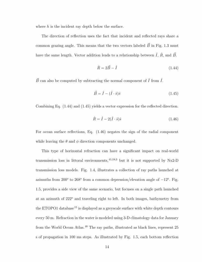
This type of horizontal refraction can have a significant impact on real-world

transmission loss in littoral environments,41;18;3 but it is not supported by Nx2-D

transmission loss models. Fig. 1.4, illustrates a collection of ray paths launched at

azimuths from 200o to 268o from a common depression/elevation angle of −12o. Fig.

1.5, provides a side view of the same scenario, but focuses on a single path launched

at an azimuth of 222o and traveling right to left. In both images, bathymetry from

the ETOPO1 database15 is displayed as a greyscale surface with white depth contours

every 50 m. Refraction in the water is modeled using 3-D climatology data for January

from the World Ocean Atlas.48 The ray paths, illustrated as black lines, represent 25

s of propagation in 100 ms steps. As illustrated by Fig. 1.5, each bottom reflection

14

Figure 1.4: 3-D refraction around a seamount (top down view, 50 m contours).

changes the depression/elevation angle of the ray path. The depression/elevation

angle increases as the ray travels up slope, and decrease as it travels down slope. For

each of these reflections, the ray path is also diverted away from the seamount peak

in the horizontal. As shown in Fig. 1.4, this broadens the acoustic shadow created

by the seamount.7

1.3.3 3-D eigenray path detection

If we think of Eqs. (1.31) through (1.38) as the time evolution of acoustic wavefronts,

then eigenray arrivals can be thought of as collisions of those wavefronts with acoustic

15

Figure 1.5: 3-D refraction around a seamount (side view, 50 m contours).

targets. Fig. 1.6 is a side view of such a collision where ~rp is the position of a single

acoustic contact, ~rnjk is the position of a point on the wavefront, dnjk is the distance

from target to each point on wavefront, ∆t is the target offset along the direction of

propagation, ∆µ is the target offset in the depression/elevation direction, and ∆ϕ is

the target offset in the azimuthal direction.

A point on the wavefront ~rnjk is the closest point of approach (CPA) for a specific

target if it has the smallest distance to that target relative to the 26 wavefront points

immediately surround it in the t, µ, and φ directions. The offset in each of these

directions is computed by expressing d2p, the square of the distance to this target, as

16

Figure 1.6: Eigenray estimation geometry (side view: ϕk direction not shown).

a second order Taylor series, relative to the CPA, in vector form.

~ρ ≡ (ρ1, ρ2, ρ3) ≡ (∆t,∆µ,∆ϕ) (1.47)

d2p ≈ ε+ ~g · ~ρ+1

2~ρ ·H ~ρ (1.48)

ε ≡ d2∣∣CPA

(1.49)

~g ≡ ∂d2

∂~ρ

∣∣CPA

(1.50)

H ≡ ∂2d2

∂~ρ2∣∣CPA

(1.51)

where ~ρ is the target offset from CPA in vector form, ~g is the gradient of squared

distance at CPA (3 elements), and H is the Hessian matrix of squared distance at

CPA (3x3). One way to solve this equation would be to search for a value of ~ρ

for which Eq. (1.48) was zero. However, since d2p is positive definite, searching for

17

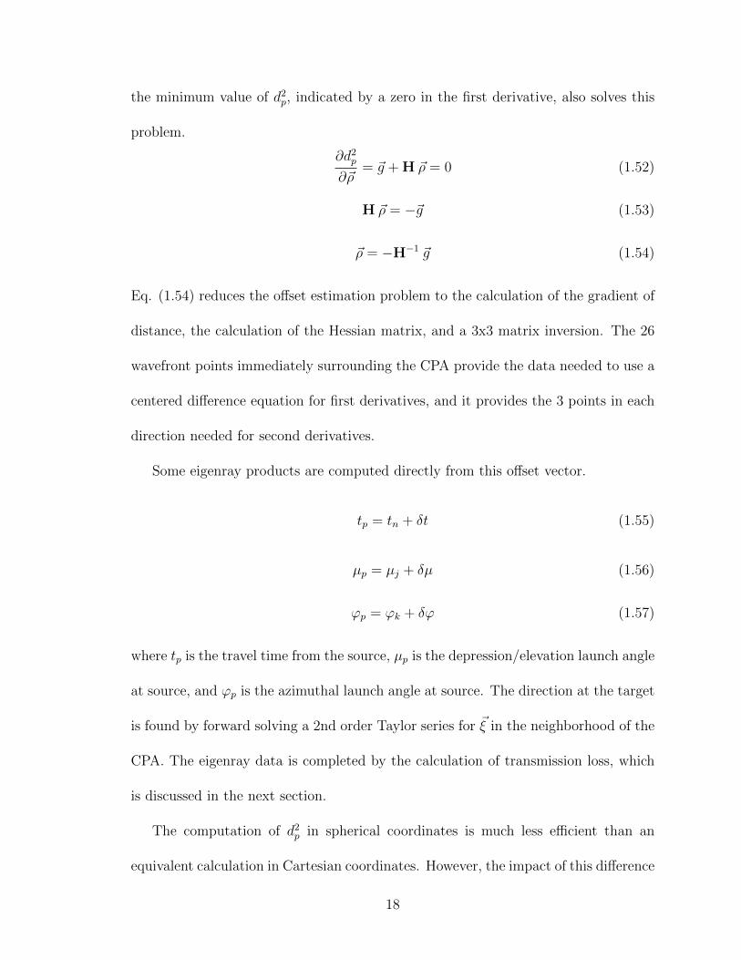
the minimum value of d2p, indicated by a zero in the first derivative, also solves this

problem.

∂d2p∂~ρ

= ~g + H ~ρ = 0 (1.52)

H ~ρ = −~g (1.53)

~ρ = −H−1 ~g (1.54)

Eq. (1.54) reduces the offset estimation problem to the calculation of the gradient of

distance, the calculation of the Hessian matrix, and a 3x3 matrix inversion. The 26

wavefront points immediately surrounding the CPA provide the data needed to use a

centered difference equation for first derivatives, and it provides the 3 points in each

direction needed for second derivatives.

Some eigenray products are computed directly from this offset vector.

tp = tn + δt (1.55)

µp = µj + δµ (1.56)

ϕp = ϕk + δϕ (1.57)

where tp is the travel time from the source, µp is the depression/elevation launch angle

at source, and ϕp is the azimuthal launch angle at source. The direction at the target

is found by forward solving a 2nd order Taylor series for ~ξ in the neighborhood of the

CPA. The eigenray data is completed by the calculation of transmission loss, which

is discussed in the next section.

The computation of d2p in spherical coordinates is much less efficient than an

equivalent calculation in Cartesian coordinates. However, the impact of this difference

18

is minimized when the number of targets is small compared to the number ray tracing

points. This is a good assumption for sonar training systems, but it makes our model

much slower than existing methods for calculating transmission loss over millions of

range, depth, and bearing combinations in tactical decision aids.

1.3.4 3-D Gaussian ray bundles

In conventional ray theory, the spreading of acoustic transmission loss is estimated by

measuring the changes in ensonified area between ray paths. The intensity across the

wavefront is inversely proportional to the change in a surface area segment compared

to its area at the source.21 The Gaussian beam approach uses a parabolic equation

approximation normal to each ray to compute spreading in the form of a Gaussian

profile for each ray.9;35;34;5 Gaussian ray bundling models, such as CASS/GRAB, use

the distance between rays (from conventional ray theory) to define the size of the

Gaussian profile for each ray.

In 2-D Gaussian beam models, the intensity at the target location is a summation

of contributions from rays above and below the eigenray target. To extend Gaussian

ray bundles to three dimensions, we use an approximation that computes independent

factors in the µ and ϕ directions (Fig. 1.7).

G(~rp) =

(j+J∑

j′=j−J

gj′(~rp)

)(k+K∑

k′=k−K

gk′(~rp)

)(1.58)

where G(~rp) is the total Gaussian ray bundle intensity at the eigenray target, (j, k) are

the index numbers of the cell containing the eigenray target, gj′ are the Gaussian ray

bundle contributions along depression/elevation direction, gk′ are the Gaussian ray

19

Figure 1.7: Gaussian ray nearest neighbors (front view: tn direction not shown).

bundle contributions along the azimuthal direction, 2J + 1 is the number of beams

used in the depression/elevation summation, and 2K + 1 is the number of beams

used in the azimuthal summation. Computing a product of independent factors is

equivalent to assuming that the width of the Gaussian ray bundles in the µ direction

represents a local average in the ϕ direction, and vice versa.

The intensity of each Gaussian ray bundle contribution is a function of the width

of each beam and the distance along the wavefront to the eigenray target, normalized

20

to the average distance across the beam at the source

gj′(~rp) =Nj′√2πw2

j′

exp

(−d2j′

2w2j′

)(1.59)

gk′(~rp) =Nk′√2πw2

k′

exp

(− d2k′

2w2k′

)(1.60)

Nj′ =

∫ ϕk′+1

ϕk′(µj′+1 − µj′) dϕ∫ ϕk′+1

ϕk′dϕ

= µj′+1 − µj′ (1.61)

Nk′ =

∫ µj′+1

µj′(ϕk′+1 − ϕk′) cos (µ) dµ∫ µj′+1

µj′dµ

=sin(µj′+1)− sin(µj′)

µj′+1 − µj′(ϕk′+1 − ϕk′) (1.62)

where wj′ and wk′ are the half-widths of the Gaussian ray bundle in the µ and ϕ

directions, and dj′ and dk′ are the distances in the µ and ϕ directions from the

Gaussian ray bundle center to the target.

GRAB45 models the frequency dependent component of the beamwidth by giving

each beam a minimum width.

w′j(f) = max (wj, 2πλ) (1.63)

where λ is the wavelength of the signal being modeled, wj is the half cell width of

beam j, and w′j(f) is the adjusted width of beam j. GRAB models beams centered

on each ray and then between each ray to create a minimum overlap of 50% between

Gaussian ray bundles.

A physical interpretation of Eq. (1.63) is that the λ term is the frequency depen-

dent Gaussian spreading that GRAB expects for rays that are infinitely close together.

The wj terms can be interpreted as the Gaussian width created by discreetly sam-

pling the launch angles. Instead of using the maximum of these two contributions,

21

our model convolves these two sources of spreading and adds their Gaussian widths

as the sum of squares.

(w′j(f))2 = (2wj)2 + (2πλ)2 (1.64)

Eq. (1.64) produces results that are similar to (1.63), but there is a smooth transition

between the domains dominated by the wj and λ terms. The factor of 2 in wj has been

artificially introduced to produce the same 50% overlap as GRAB without doubling

the number of beam calculations. Normalizing Eq. (1.59) and (1.60) by the combined

effect of both spreading sources conserves energy across the wavefront.

1.4 Test Results

Although the primary goal of this research is to develop a transmission loss model

that reduces computational burden, the training systems also require an accurate

representation of real-world phenomena. This section presents the results of several

key accuracy tests including for ray path refraction accuracy using a Munk profile

(Section 3.1), Gaussian beam projection into the shadow zone for an n2 linear profile

(Section 3.2), and horizontal refraction from a 3-D analytic wedge (Section 3.3). An

comparison to CASS/GRAB executions times is provided in Section 3.4.

1.4.1 Refraction accuracy benchmark

Because our model’s calculation of transmission loss is closely tied to the location

of ray paths, refraction accuracy is an important element of its overall accuracy.

Because the use of spherical coordinates incorporates the radius of the Earth (a

22

large number) into the radial coordinate in Eqs. 1.31 through 1.36, we need to

address concerns that our approach would suffer from numerical accuracy problems.

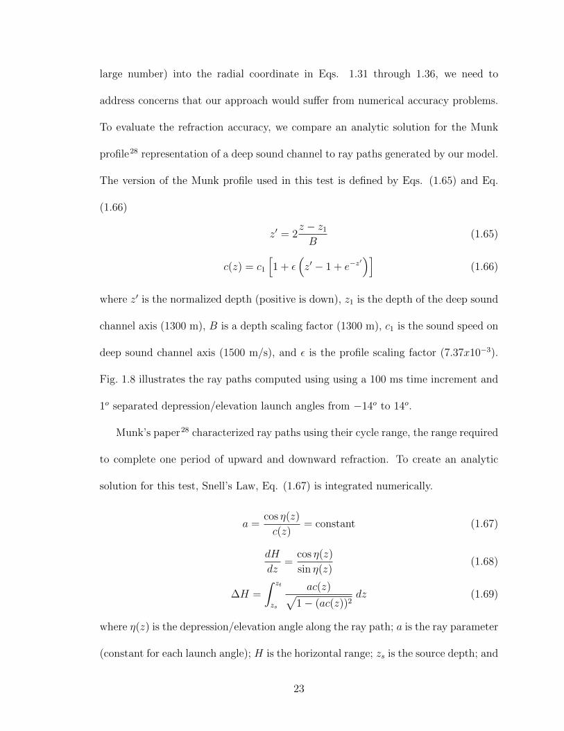
To evaluate the refraction accuracy, we compare an analytic solution for the Munk

profile28 representation of a deep sound channel to ray paths generated by our model.

The version of the Munk profile used in this test is defined by Eqs. (1.65) and Eq.

(1.66)

z′ = 2z − z1B

(1.65)

c(z) = c1

[1 + ε

(z′ − 1 + e−z

′)]

(1.66)

where z′ is the normalized depth (positive is down), z1 is the depth of the deep sound

channel axis (1300 m), B is a depth scaling factor (1300 m), c1 is the sound speed on

deep sound channel axis (1500 m/s), and ε is the profile scaling factor (7.37x10−3).

Fig. 1.8 illustrates the ray paths computed using using a 100 ms time increment and

1o separated depression/elevation launch angles from −14o to 14o.

Munk’s paper28 characterized ray paths using their cycle range, the range required

to complete one period of upward and downward refraction. To create an analytic

solution for this test, Snell’s Law, Eq. (1.67) is integrated numerically.

a =cos η(z)

c(z)= constant (1.67)

dH

dz=

cos η(z)

sin η(z)(1.68)

∆H =

∫ zt

zs

ac(z)√1− (ac(z))2

dz (1.69)

where η(z) is the depression/elevation angle along the ray path; a is the ray parameter

(constant for each launch angle); H is the horizontal range; zs is the source depth; and

23

1500 1550−5000

−4500

−4000

−3500

−3000

−2500

−2000

−1500

−1000

−500

0

Speed (m/s)

Depth

(m

)

0 20 40 60 80 100 120 140Range (km)

Figure 1.8: Munk profile (left panel) and modeled ray paths (right panel).

zt is the target depth. Although these integrals only apply between the source and

the first vertex or reflection, paths out to any range can be constructed by repeating

this process after the vertex or reflection.

Pekeris’ modified index of refraction, shown in Eq. (1.70), allows Cartesian mod-

els, like the Munk profile, to incorporate earth curvature effects into their calcula-

tions.33 This process can also be inverted, as shown in Eq. (1.71), to allow spherical

models, like ours, be compared to flat earth benchmarks.

n(z) =r

R

n(r)

n(R), (1.70)

24

c(r) =r

Rc(z) , (1.71)

where R is the radius of earth’s curvature in this area of operations; r is the radial

distance from the center of curvature (positive is up); z = R − r is the depth below

the ocean surface (positive is down); n(r) is original index of refraction in spherical

coordinates, n(z) is adjusted index of refraction in Cartesian coordinates, c(z) is the

benchmark’s speed of sound in Cartesian coordinates, c(r) is thee adjusted index of

refraction in spherical coordinates.

Fig. 1.9 compares our model’s cycle range to those computed using Eqs. (1.69).

Our model deviates from the analytic solution by a maximum of -8.62 m at a range

of 129.95 km (0.007% error). However, 50 out of 58 samples (86%) exhibit errors less

than ±2 m (0.002% error). Ray paths that are initially launched toward the surface,

where the sound speed gradient is highest, have consistently larger errors than paths

that were launched down. Because the use of spherical coordinates incorporates the

radius of the Earth (a large number) into all radial values, we initially had concerns

that our approach would suffer from numerical accuracy problems. Our results for

refraction accuracy indicate that those concerns are unfounded. At this time, it does

not appear that incorporation the radius of the Earth into the radial coordinate in

Eqs. 1.31 through 1.36 causes significant accuracy problems.

1.4.2 2-D transmission loss benchmark

To compare the accuracy of our transmission loss estimates to existing 2-D Gaussian

beam models, coherent transmission loss is calculated at the edge of a shadow zone

25

0 20 40 60 80 100 120 140−10

−8

−6

−4

−2

0

2

Range (km)

Ra

ng

e E

rro

r (m

)

Launched Up

Launched Down

Figure 1.9: Cycle range difference between model and analytic solution for Munkprofile ray traces.

using the Pedersen and Gordon n2 linear test case.32

c(z) =c0√

1 + 2g0c0z

(1.72)

where c0 is the sound speed at the ocean surface (1550 m/s) and g0 is the sound

speed gradient at at the ocean surface (1.2 s−1). Fig. 1.10 illustrates ray paths;

both the surface and direct paths encounter a shadow zone at ranges beyond 880

m. Conventional ray theory predicts that no energy enters the shadow zone. This

benchmark has been used in several other 2-D Gaussian beam models45;34 to validate

their ability to predict the smooth transition predicted by the analytic solution.

26

14001500−200

−180

−160

−140

−120

−100

−80

−60

−40

−20

0

Speed (m/s)

Depth

(m

)

0 0.2 0.4 0.6 0.8 1 1.2Range (km)

Figure 1.10: Pederson profile (left panel) and modeled ray paths (right panel).

Fig. 1.11 illustrates the computed transmission losses for this scenario at 2000

Hz. The Fast Field Program (FFP) wavenumber integration technique14;6 generates

the solution labeled theory in this figure. The GRAB solution is computed using

the Comprehensive Acoustic System Simulation Model (CASS) version 4.2.17 These

solutions are compared to our model, labeled ”New” in Fig. 1.10. In this comparison

Eq. (1.71) is used to remove the effect of the Earth’s curvature from the ”New”

results. Prior to the shadow zone, all three models produce similar results. Although

the loss predicted by our model is slightly higher than FFP in the shadow zone,

its results are similar to the ones produced by GRAB. In both cases, the slight rise

27

0.5 0.55 0.6 0.65 0.7 0.75 0.8 0.85 0.9 0.95 1−80

−75

−70

−65

−60

−55

−50

−45

−40

Range (km)

Pro

pagation L

oss (

dB

)

New

GRAB

theory

Figure 1.11: Gaussian beam projection into the shadow zone for an n2 linear profileat 2000 Hz.

in the coherent transmission loss appears to be caused by phase inaccuracies in the

multi-path travel times predicted in the shadow zone.

1.4.3 3-D transmission loss benchmark

To demonstrate 3-D effects in transmission loss, we examine the analytic solutions

for a 3-D wedge. In this scenario, receivers are at the same distance from the wedge

apex as the source, but offset in range across the slope. In an 2-D model, these

receivers appear to exist in an environment of constant depth. Because the 3-D

28

solution horizontally refracts acoustic energy down the slope, the 3-D solution has

higher transmission loss, as a function of range across the slope, than the 2-D model.

Figure 1.12: Geometry for method of images in a 3-D wedge.

Using the method of images, we assume that each reflection gives rise to a source

image, and that these images lie on a circle centered on the apex of the wedge. This

29

derivation is similar to the Deane/Buckingham model13, but it simplifies that model

by assuming that interface reflection coefficients are limited to 1. This simplification

creates an analytic solution that is accurate at higher frequencies.

Fig. 1.12 is a cross-slope view of the 3-D wedge showing each of the image sources

and each virtual interface. In this illustration, surface interfaces are shown with a

dashed line, bottom interfaces are shown with a dot-dashed line, and source images

are shown as dots along the circumference of a circle whose radius is defined by the

original distance of the source from the apex. The complex pressure at each receiver

location is a sum of spherical wave contributions from each source image. If we assume

that the reflection coefficient is +1 at the bottom and -1 at the surface.

pq =nmax∑

n=−nmax

n∑m=n−1

(−1)meikRn,m,q/Rn,m,q (1.73)

where n is the number of bottom reflections for source image, negative if above surface;

m is the number of surface reflections for source image, negative if above surface; nmax

is the maximum number of bottom bounces; ~sn,m is location of each source image; q

is the index number for each receiver; ~rq is the location of each receiver; Rn,m,q is the

slant range from each source image to each receiver; c is the speed of sound in water;

f is the signal frequency; k is the acoustic wave number = 2πf/c; and pq is the total

complex pressure for each receiver.

To compute Rn,m,q, we define a cylindrical coordinate system whose axis travels

along the wedge apex: Rs is the slant range of original source from the wedge apex;

αs is the angle of original source down from the ocean surface; αn,m is the angle of

30

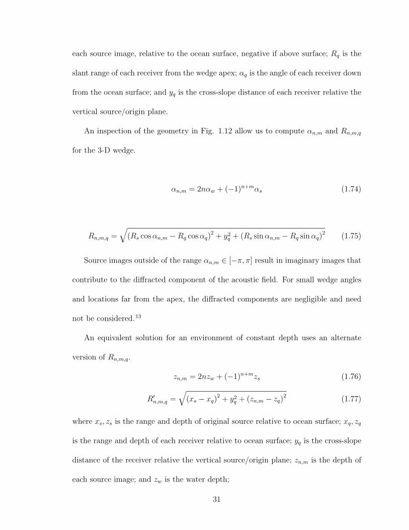
each source image, relative to the ocean surface, negative if above surface; Rq is the

slant range of each receiver from the wedge apex; αq is the angle of each receiver down

from the ocean surface; and yq is the cross-slope distance of each receiver relative the

vertical source/origin plane.

An inspection of the geometry in Fig. 1.12 allow us to compute αn,m and Rn,m,q

for the 3-D wedge.

αn,m = 2nαw + (−1)n+mαs (1.74)

Rn,m,q =√

(Rs cosαn,m −Rq cosαq)2 + y2q + (Rs sinαn,m −Rq sinαq)

2 (1.75)

Source images outside of the range αn,m ∈ [−π, π] result in imaginary images that

contribute to the diffracted component of the acoustic field. For small wedge angles

and locations far from the apex, the diffracted components are negligible and need

not be considered.13

An equivalent solution for an environment of constant depth uses an alternate

version of Rn,m,q.

zn,m = 2nzw + (−1)n+mzs (1.76)

R′n,m,q =√

(xs − xq)2 + y2q + (zn,m − zq)2 (1.77)

where xs, zs is the range and depth of original source relative to ocean surface; xq, zq

is the range and depth of each receiver relative to ocean surface; yq is the cross-slope

distance of the receiver relative the vertical source/origin plane; zn,m is the depth of

each source image; and zw is the water depth;

31

Because our model uses geodetic coordinates, the simple wedge used in our analytic

solution can only be approximated in this comparison. On a round earth, an interface

with constant slope is a curved surface instead of a plane. To minimize the impact

of this curvature, the wide wedge angle scenario is used to shorten the range over

which 3-D effects can be observed. The source and receivers are placed at a depth of

100 meters at the Equator. The water depth at this point is set to 200 meters and

the bottom slope is a constant 21o, sloping down to the north, at all latitudes and

longitudes. This definition orients the wedge in Fig. 1.12 such that the x-direction is

north, the y-direction is east, and the z-direction is down. Receivers are placed east

of the source, along the y-direction, at varying cross slope ranges.

Fig. 1.13 compares of our model to the analytic solution for a 3-D wedge. It

also illustrates the analytic solution and the CASS/GRAB v4.2 prediction for an

equivalent 2-D ocean with a constant depth of 200 meters. As predicted, the analytic

solution for a simple 3-D wedge has higher transmission loss as a function of range

across the slope than 2-D models of this same scenario. Our 3-D model accurately

predicts this effect.

1.4.4 Computational efficiency

A key premise of this paper is that, when target/sensor geometries are constantly

evolving, it is more computationally efficient to perform acoustic transmission loss in

the latitude, longitude, altitude coordinates of the underlying environmental databases,

than it is to convert the 3-D environments into a series of Nx2-D radials. To evaluate

32

Cross Slope Range (km)

0 0.5 1 1.5 2 2.5 3 3.5 4 4.5 5

Tra

nsm

issio

n L

oss (

dB

)

-70

-65

-60

-55

-50

-45

-40

-35

-30

Flat Bottom

3-D Wedge

GRAB

New

Figure 1.13: Incoherent transmission loss at 2000 Hz for 3-D wedge and flat bottom.

this premise, a CASS scenario that interpolates radials from a 3-D data set was mod-

ified to compute transmission loss for a variable number of targets. The ”std14” test

that is distributed with CASS includes a grid of sound speeds and bottom depths,

in latitude and longitude coordinates, for an area between 16:12N to 24:36N and

164:42W to 155:24W. The source is located at 19:31.2N 160:30.0W, at a depth of 200

m. We modified this test to include multiple targets, defined at a depth of 100 m and

a range 100 km from the source, evenly spaced in azimuth. CASS constructs a radial

for each target, and then computes transmission loss using a depression/elevation

ray fan of +89o to −89o using 1o increments. An equivalent result from our model

33

propagates a wavefront for 80 seconds using a 100 ms time step, using 181 depres-

sion/elevation angles −90o to +90o, and 25 azimuthal launch angles from 0o to 360o.

Execution time is measured as a function of the number of targets.

Number of Targets

0 20 40 60 80 100

Tim

e (

s)

0

5

10

15

20

25

30

35

40

45

50

GRAB

New

Figure 1.14: Comparison to CASS/GRAB executions times as a function of numberof targets.

Fig. 1.14 illustrates the computational speeds of the models, run on a Dell Latitude

Laptop E6520 Intel i5-2540M CPU @2.60GHz, with a variable number of targets

from 0 to 100, in increments of 10. The ordinal axis illustrates the time required

to compute transmission loss for all targets on this hardware. The time required

to compute transmission loss is roughly linear for both models. The GRAB model

requires approximately 476 ms per target. The measured speed of our model is

34

approximately 3.07 seconds plus 42 ms per target. For small numbers of targets,

GRAB is faster, because our model has to propagate the wavefront in all directions

for 80 seconds, regardless of the number of targets. GRAB only needs to construct

2-D radials if a target is actually present. However, as the number of targets grows

large, our model is faster because it has a much less computational overhead on a

per target basis. The crossover point for this scenario appears to be approximately 4

targets. For 100 targets, our model is over 6 times faster than GRAB and 10 times

faster than the speed of sound.

1.5 Conclusions

This paper has defined a 3-D Gaussian ray bundling model based on the same lati-

tude, longitude, altitude coordinates used in the underlying environmental databases.

The development of our model incorporates an implementation of 3-D refraction, 3-D

interface reflection, 3-D eigenray detection, and a 3-D variant of Gaussian ray bun-

dles. Testing to date indicates that this approach has accuracy at least as good as

CASS/GRAB v4.2, but with improved execution speed benefits for large numbers of

targets, and 3-D transmission loss effects.

Wavefront Queue 3-D (WaveQ3D) is a C++ implementation of this model. WaveQ3D

is freely available to the research community as an open-source product distributed as

part of the Under Sea Modeling Library (USML). Formal releases and test results are

distributed through the Ocean Acoustics Library,31 a web site used by the U.S. Office

of Naval Research as a means of publishing software of general use to the international

35

ocean acoustics community. Software developers can also participate directly in the

WaveQ3D development process through the Under Sea Modeling Library project on

the GitHub repository hosting service.43 Documentation on the application program-

mer’s interface (API) for this software and additional test results are also available

from both sources.

1.6 Acknowledgments

Testing and productization of this model were funded by the High Fidelity Active

Sonar Training (HiFAST) Project at the U.S. Office of Naval Research.

36

Manuscript 2

Investigation of horizontal refraction on Florida Straits continental shelf using a

three-dimensional Gaussian ray bundling model

by

Sean M. Reilly and Gopu R. Potty

Ocean Engineering Department, University of Rhode Island

Narragansett, Rhode Island 02882

David Thibaudeau

AEgis Technologies Group, Inc.

North Kingstown, Rhode Island 02852

Submitted to the JASA Express Letters, March 2016

37

2.1 Abstract

Acoustic transmission loss measurements from the Calibration Operations (CALOPS)

experiment for the Shallow Water Array Performance (SWAP) program included

horizontally refracted returns that were as much as 30 degrees away from the true

bearing between source and receiver. In many cases, the in-shore refracted path

was as much as 20 dB stronger than the true bearing path. In this study CALOPS

transmission loss measurements at 415 Hz are compared to predictions from a 3D

Gaussian Ray bundling model. The geoacoustic model that provides good model-

data comparison is consistent with the geologic and sediment core data collected at

the location but differs slightly from the bottom model used at lower frequencies (206

Hz and 52.5 Hz) in a previous study.

2.2 Introduction

Several investigators have recently studied the presence of strong 3D propagation ef-

fects in experimental data on the continental shelf in the Florida Straits area.30;22;41;19;20;4

Acoustic transmission loss measurements from the Calibration Operations (CALOPS)

experiment for the Shallow Water Array Performance (SWAP) program included

horizontally refracted returns that were as much as 30 degrees away from the true

bearing between source and receiver.19 In many cases, the in-shore refracted path

was as much as 20 dB stronger than the true bearing path. CALOPS transmis-

sion loss measurements at 206 Hz20 and 52.5 Hz4 have already been analyzed using

38

3D normal model/parabolic equation hybrid models. In the present study, measure-

ments at 415 Hz are used to evaluate the 3D capabilities of the Wavefront Queue

3D (WaveQ3D) transmission loss model. WaveQ3D is a 3D Gaussian ray bundling

model that implements propagation in geodetic coordinates.38 This model supports

3D effects including horizontal refraction in sloped environments, and in this study

we investigate this capability of the model.

2.3 Experiment

Figure 2.1 provides an overview of the geometry of the CALOPS experiment and

the environment for this location, as specified in the Heaney19 and Ballard4 studies.

The experiment used a horizontal line array of 120 elements, with half wavelength

spacing at 450 Hz (1.75 m). This receiver is located on the bottom at 26:01:18N

79:59:26W and oriented such that the broadside beam points toward 8o relative to

true north. As illustrate by the white dashed line in Figure 2.1(a), the source in

Run 1N was towed along a heading of 8o true away from the receiver. This source,

towed at a depth of 100 m, used a combination of 60 second long CW pulses, with

frequencies of 24, 52.5, 106, 206, and 415 Hz and a 30-s multi-band set of five linear

frequency modulated (LFM) pulses in the frequency bands 20-50, 50-100, 120-180,

200-300, and 320-420 Hz. The source levels varied from 170.5 dB//µPa@1m at 52.5

Hz to 171.0 dB//µPa@1m at 415 Hz. Transmission loss measurements were made at

ranges between 3 and 80 km

The measured signal level is extracted from the frequency spectrum peak for each

39

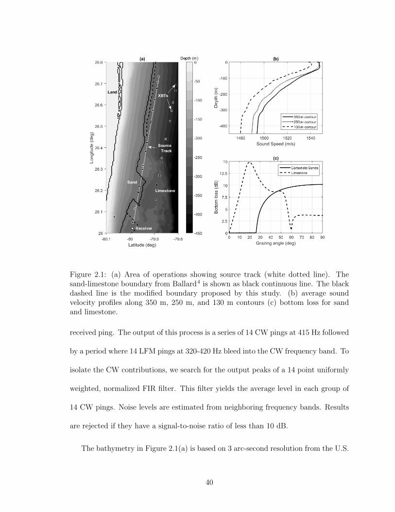
Figure 2.1: (a) Area of operations showing source track (white dotted line). Thesand-limestone boundary from Ballard4 is shown as black continuous line. The blackdashed line is the modified boundary proposed by this study. (b) average soundvelocity profiles along 350 m, 250 m, and 130 m contours (c) bottom loss for sandand limestone.

received ping. The output of this process is a series of 14 CW pings at 415 Hz followed

by a period where 14 LFM pings at 320-420 Hz bleed into the CW frequency band. To

isolate the CW contributions, we search for the output peaks of a 14 point uniformly

weighted, normalized FIR filter. This filter yields the average level in each group of

14 CW pings. Noise levels are estimated from neighboring frequency bands. Results

are rejected if they have a signal-to-noise ratio of less than 10 dB.

The bathymetry in Figure 2.1(a) is based on 3 arc-second resolution from the U.S.

40

Coastal Relief Model (CRM).12 The grey scale has contours at 25 m increments. The

black squares are locations where expendable bathythermographs (XBTs) were used

to estimate the in-situ sound velocity profile. For this analysis, we averaged XBT

measurements across the 350 m, 250 m, and 130 m contours and extended them to

the bottom using Data Interpolating Empirical Orthogonal Functions (DINEOF).1;2

Panel (b) illustrates the averaged sounds speeds, which increase in deeper areas under

the influence of the warm waters of the Florida Current. To create a 3D profile, the

averaged results are interpolated onto a 3D grid of latitude/longitude/depth locations

based on their distance perpendicular to the source ship track.

The bottom loss shown in Figure 2.1(c) is a plane wave reflection coefficient derived

from Ballard’s analysis of geophysical measurements in this area.4 The sand bottom

loss has a compressional wave speed of 1676 m/s, compressional attenuation of 0.01

(dB/λ), and a density of 1.70 (g/cm3). The limestone bottom loss has a compressional

wave speed of 3000 m/s, compressional attenuation of 0.10 (dB/λ), and a density of

2.40 (g/cm3), a shear speed of 1430 m/s, and a shear attenuation of 0.20 (dB/λ). The

limestone bottom has high bottom loss, but the carbonate sand sediments are almost

perfectly reflective at the low grazing angles that influence long range propagation.

Ballard reports that the bottom is bare limestone below the 236 m isobaths, where

loose sediments have been scoured away by the Florida Current. At shallower depths,

carbonate sand layers cover the bottom. Ballard also reports an area near 26:12N

79:58W where echo sounder measurements along the source track indicate that a deep

pool of sediment has formed between two sea mounts. Ballard’s boundary between the

41

sand and limestone areas is shown by the black line in panel (a). Ballard states that

the reported location of this boundary likely varies along the shelf and its position is

difficult to fully characterize with the limited data available.4 Our modeling results

discussed in Section III indicate that the geoacoustic model which provides good

model-data comparison has this boundary shifted slightly towards deeper waters as

shown in Figure 2.1(a) (dashed lines).

2.4 Comparison of measurements with model pre-

dictions

The environmental conditions and geometry discussed in Section II were used for

the 3D modeling of the acoustic propagation for comparison with the measurements.

Results from two iterations of modeling are presented in this section. The only

difference in inputs between these two model runs is the location of the sand-limestone

boundary. The first model run was performed with the location of the sand-limestone

boundary as discussed in Ballard4 i.e. along the 236 m isobath. These model results

at 415 Hz did not compare well with the observations. After a rigorous parametric

study we identified the location of the sand-limestone boundary plays a critical role in

determining the transmission loss. Hence we repeated our model runs with a modified

location of the sand-limestone boundary which produced better agreement with the

data. The details of these two model runs and the comparisons of the model results

with the data are described in more detail in this Section.

To model this scenario in WaveQ3D, wavefronts are propagated from the receiver

42

to a series of target locations along the source track. WaveQ3D models propagation as

the time evolution of ray paths that are launched across a fan of depression/elevation

and azimuthal launch angles. Transmission loss is modeled as a sum of Gaussian

contributions across the wavefront at each point where the wavefront intersects with

a target.38

The model indicates that ray paths are trapped along the bottom by the downward

refracting nature of the sound velocity profile; this results in large numbers of bottom

reflections along every path. Rays that are launched east of the ship’s track travel

at nearly constant azimuth, but they suffer from significant attenuation each time

that they reflect off of the limestone. Ray paths west of the track (up the slope) are

horizontally refracted back toward the source, but suffer from little or no reflection

loss, because of the sandy bottom.

At each source location, WaveQ3D computes a series of eigenrays that each in-

cludes transmission loss amplitude and phase, depression/elevation and azimuthal

launch angles, depression/elevation and azimuthal arrival angles, and travel time. To

model the detection process, eigenrays are scaled by the beam pattern gain for each

receiver beam and incoherently summed to estimate the average receive level. The

strongest beam in the direct and in-shore regions is reported as the transmission loss

and bearing at each range. Figure 2.2(a) illustrates transmission loss as a function

of array bearing for each source range. The contributions between 0 and 40 km at

a bearing of 8o are referred to by Heaney19 as the direct path contributions, even

though they suffer from multiple bottom bounces. The in-shore paths, created by

43

horizontal refraction off of the continental slope, come in at a bearing of −80o at 3

km and shift to −18o at ranges of 60 km.

Figure 2.2: Compare modeled horizontal refraction to measured data.

Figure 2.2 (b) and (c) shows the comparison between measured and modeled

results. The model accurately predicts the presence of the in-shore path, but over

estimates its arrival angle at ranges below 20 km. The modeled transmission loss

values for the direct paths are slightly weaker than the measured levels at ranges up

to 40 km, but the in-shore levels appear to follow the measured transmission loss. At

ranges beyond 40 km, the model significantly under predicts the strength of in-shore

paths.

44

Figure 2.3: Modeled horizontal refraction with thin sediment layers.

We investigated the sensitivity of the modeling result to different parameters and

found that the modeled transmission loss levels are most sensitive to the placement of

the boundary between the sandy slope and the limestone shelf. Figure 2.3 illustrates

results for an adjusted placement of the sand/limestone boundary that is a better

fit to measured transmission loss. The first adjustment, shown as a dashed line in

Figure 2.1(a), places an additional sand pool in the area around the receiver. This

adjustment is supported by the fact that array was placed in a relatively flat region

which is several kilometers wide, and echo sounder measurements indicate a sand layer

of up to a 5 m thickness in the area along the source track and south of 26:02N.4 The

45

second adjustment shifts the sand/limestone boundary north of 26:27N from a depth

of 236 m to 255 m. In this area, a sand layer could overlay the limestone without

contradicting the echo sounder measurements, which indicate little or no coverage

along the ship track in this area.

As shown in Figure 2.3, the agreement between transmission loss measurements is

very good when the spatial distribution of the bottom properties is slightly modified

(consistent with the core data and echo sounder measurements). The addition of

a sand pool near the receiver significantly improves the fit of the modeled direct

path transmission loss to measurements. It also significantly increases the strength

of the modeled in-shore paths for ranges between 10 and 50 km. The movement of

sand/limestone boundary north of 26:02N reduces the rate at which transmission loss

decreases as a function of range beyond 50 km. In the high frequency approximation,

bottom loss values are be limited to an interface plane-wave reflection coefficient.

It should be noted that the 415 Hz measurements used in this study may be more

sensitive to surficial sediments than measurements at 52.5 Hz and 206 Hz. This

sensitivity difference could explain our need to change the effective location of the

boundary between sand and limestone bottom loss provinces.

2.5 Acknowledgments

This work would not have been possible without the sea test data and sage advice

provided by Dr. Kevin Heaney, Dr. Megan Ballard, and their associates. The authors

would like to also thank Dr. James Miller for his help and insight on the sensitivity

46

analysis of modeling results. Parts of this effort were funded by the High Fidelity

Active Sonar Training (HiFAST) Project at the U.S. Office of Naval Research.

47

Manuscript 3

How the U.S Navy is Migrating from Legacy/Large Footprint to Low Cost/Small

Footprint Sonar Simulation Systems

by

Sean M. Reilly

AEgis Technologies Group, Inc.

North Kingstown, Rhode Island 02852

Jonathan Glass

Naval Air Warfare Center Training Systems Division

Orlando, FL 32816

Published in the Interservice/Industry Training, Simulation and Education

Conference (I/ITSEC) Proceeding, Paper No. 14090, December 2014

48

3.1 Abstract

This paper describes the migration process undertaken by the US Navy to migrate

from legacy, large footprint mainframe computer-based sonar simulation systems to

next-generation sonar simulation systems with a smaller footprint, lower costs and

better accuracy than the legacy models. The paper will describe the development

efforts to create a faster and more accurate acoustic transmission loss (TL) and re-

verberation model for sonar simulation/stimulation systems in littoral environments

based on ray theory for active sonar frequencies (above 1000 Hz). The paper also

describes how the next-generation model augments ray theory with Gaussian beam

techniques (based on the Gaussian Ray Bundling or GRAB), which enables simula-

tion of frequencies as low as 150 Hz. The paper will detail the integration challenges

faced by the US Navy to migrate from the legacy models to the next-generation

sonar simulation model into the Navy’s Live Virtual Constructive Modeling and Sim-

ulation (LVCMS) product line that includes PACT3, BATTT, and EFAAS simula-

tors/simulations. The paper will also describe the results of these integration efforts,

including the ability to provide trainees with improved training via more complex

scenarios in the LVCMS training suite without increasing their hardware costs or

footprint.

49

3.2 Introduction

The Live, Virtual, Constructive Modeling and Simulation (LVCMS)/Anti-Submarine

Warfare Virtual At-Sea Training Systems (ASW VAST) is a suite of networked, PC-

based deployable trainers designed to support integrated and coordinated ASW tac-

tical training using Joint Semi Automated Forces (JSAF) Navy Training Baseline

(NTB) simulation.29 The current training system configuration is comprised of per-

sonal computers (PC), each PC system representing a mission training station in a

particular aircraft (i.e. SH-608, SH-60F, P-3C) or shipboard system that, when in a

networked environment, allow for integrated mission training. Currently, the LVCMS

and ASW VAST family of training systems include:

• Mission Rehearsal Tactical Team Trainer (MRT3),

• Bravo Aircrew Tactical Team Trainer (BATTT),

• Bravo Romeo Acoustic Stimulation System (BRASS),

• High Fidelity Active Sonar Training Command (HIFAST CMD),

• P-3 Air Crew Tactical Team Trainer (PACT3),

• Virtual Maintenance Performance Aide (VMPA),

• Virtual Anti-Submarine Warfare (ASW)/Anti-Surface Warfare (ASUW) Tacti-

cal Air Controller (VASTAC),

• Effective Active Acoustic Simulation/Stimulation (EFAAS),

50

• Sonobuoy Acoustic Training System (SATS),

• Common Distributed Mission Training Station (CDMTS), and

• Tactical Warfare Instructor Support Environment (TACWISE).

Each of these systems supports a distributed simulation interface to the Fleet Syn-

thetic Training (FST). FST exercises use distributed simulation to conduct in-port

exercises at the Joint (FST-J), Group Command (FST-GC), Warfare Commander

(FST-WC), and Unit (FST-U) levels. These exercises are used as part of Fleet Readi-

ness Training Plan (FRTP) to certify the readiness of ships, submarines, aircraft, and

commanders for deployment. When Navy assets are at-sea, they conduct operations;

when they are in port, they train for the next operation. The Navy Continuous Train-

ing Environment (NCTE) is the hardware/software architecture that brings together

the training systems for individual ships, submarines, aircraft, and commanders into a

common virtual environment. Each combat system builds their own training system,

and the NCTE integrates these systems across wide area networks.

Coordinated anti-submarine warfare (ASW) depends on a complex mosaic of

diverse capabilities in a highly variable physical environment.27 No single ASW plat-

form, system, or weapon will work all the time. The undersea environment demand a

multi-disciplinary approach, subsuming intelligence, oceanography, surveillance and

cueing, multiple sensors and sensor technologies, coordinated multi-platform oper-

ations, and underwater weapons. Low-cost, deployable ASW training increase the

opportunities for sonar technicians and commanders, from the Air Tactical Officers

all the way up to the Theater ASW Commander, to practice playing together as a

51

Figure 3.1: Fleet Synthetic Training Concept

team.

One of the key technological hurdles to the engineering of such systems is creating

sonar simulations that realistically represent the acoustic characteristics of the ocean

environment, for dynamic scenarios, on limited hardware, in real-time. Sonar realism

is a key element in teaching sonar technicians to recognize and react to the acoustic

phenomena that allow them to detect, track, classify, localize, and engage submarine

targets. In littoral environments, the sonar is often cluttered with large numbers of

false targets, and accurate portrayal of these contacts is critical in teaching sonar

technicians to discard false detections. False targets can be a particularly difficult

problem for active sonar systems because these systems provide more limited classi-

fication data than passive systems. In this case, improving the quantity of acoustic

contacts directly impacts the quality of the training. Training realism suffers when

52

only a small number of acoustic contacts are presented to the sonar operator. Unfor-

tunately, most efforts to increase the number of realistic contacts have relied on the

use of massively parallel computing systems with high acquisition costs.

Figure 3.2: Mission Rehearsal Tactical Team Trainer (MRT3)

The Wavefront Queue 3-D (WaveQ3D) model is a research effort to create fast

and accurate acoustic transmission loss (TL) eigenrays, in littoral environments, for

sonar simulation/stimulation systems. The new model is based on ray theory because

Parabolic Equation and Normal Mode models run prohibitively slow at active sonar

frequencies above 1000 Hz, where the number of propagating modes is large. To

extend applicability to lower frequencies, the new model augments ray theory with

Gaussian beam techniques based on the Gaussian Ray Bundling (GRAB),45 which is

certified for use down to 150 Hz. Our computation speed goal is to model one-way

transmission loss for 100 targets on a single core of an average laptop.

3.3 Wavefront Queue 3-D Model

The key innovation in the development of the new model was the recognition that

the requirements of sonar training systems are much different from those of tactical

53

decision aids. Sonar tactical decision aids (TDAs) are used at-sea to provide the sonar

team with an ability to analyze the impact of ocean conditions on the likelihood

of submarine detection. Because the behavior of the target cannot be predicted

ahead of time, the TDAs must be optimized to perform their calculations over a

wide variety of ranges, bearing, and depths. For many models, this optimization

requires a transformation of oceanographic data onto a series of 2-D radials. This

transformation allows the transmission loss calculations to use a simple Cartesian

coordinate system and produce results at multiple ranges and depths. The amount

of data to be analyzed is large, but such predictions are only generated a few times

per day.

Sonar training systems must solve a very different problem. The ground truth

locations of the targets are known by the sonar simulation, the behaviors of those

targets react to trainee actions in real-time, and the sonar displays must display

those reactions in real-time. The computational benefit of transforming into a series

of 2-D radials is lost if each of those radials is only used to create a single transmission

loss for the current location of each target. If the sonar simulation attempts to regain

this advantage by interpolating between a small number of fixed radials, accuracy is

lost. The amount of data to be analyzed is much smaller than in the TDA case, but

predictions must be generated in real time for a dynamically evolving scenario.

The new model takes a new approach by leaving the data in latitude, longitude,

and depth coordinates, and changing the transmission loss equations to operate in

this 3-D coordinate system. The oceanographic data for large areas is cached in

memory and re-used for multiple sensors. As illustrated in Figure 3.3, oceanographic

54

Figure 3.3: Extract 2-D radial and compute transmission loss

data from multiple sources, including open access data from the National Oceanic

and Atmospheric Administration (NOAA), U.S. Navy standard databases like the

Oceanographic and Atmospheric Master Library (OAML), dynamically evolving grid-

ded data from NCTE, and live forecasts from the Fleet Numerical Meteorology and

Oceanography Center (FNMOC), is combined to meet the needs of specific training

exercises. Motion of the sensors does not require a change to the underlying environ-

ment. The premise of this approach is that, when scenario geometries are constantly

evolving, it is more computationally efficient to perform acoustic transmission loss

(TL) in spherical Earth coordinates than it is to convert the world into a series of

2-D Cartesian slices.

WaveQ3D models acoustic propagation as collection of wavefronts that move

through the environment in increments of time. A single wavefront supports all

55

Figure 3.4: Caching data in latitude, longitude, and depth coordinates

of the acoustics contacts relevant to a given sensor. When the wavefront collides with

an acoustic target, the model generates an eigenray that specifies the transmission

loss, travel time, and source/receiver angles of the ensonification. The new model can

collect the eigenrays for all acoustic contacts into a single container, or it can pass

them back to the simulation as they happen. This second mode of operation allows

the training simulation to start signal processing on nearby targets before processing

has been completed on distant targets.

In conventional ray theory, the spreading of acoustic propagation loss is esti-

mated by measuring the changes in ensonified area between ray paths. The intensity

across the wavefront is inversely proportional to the change in a surface area segment

compared to its area at the source. The Gaussian beam approach uses dynamic ray

56

equations to compute the divergence of the acoustic field normal to the path of propa-

gation. The U.S. Navy’s Comprehensive Acoustic Simulation System / Gaussian Ray

Bundle (CASS/GRAB) model takes a different approach and estimates the diver-

gence directly from the shapes of the wavefront. This reduces the computational cost

of transmission loss calculations. The WaveQ3D model adapts the 2-D CASS/GRAB

approach for estimating divergence into 3-D environment.

3.4 Speed and Accuracy Testing

To evaluate the speed potential of the new model, a scenario was developed to com-

pare speeds to existing Navy models for high fidelity TDAs. One challenge in de-

veloping such a scenario was finding a case in which the speed of the TDA model

included the formation of 2-D radials. Fortunately, one of test routines that come

with CASS/GRAB is a case where the bathymetry and sound speed are extracted

directly from grids specified in latitude and longitude coordinates (Express Test 14).

This test was modified to create a variable number of targets, 100 km from the source,

evenly spaced in azimuth. An equivalent scenario was then created using WaveQ3D.

The timing tests were run on a Dell Latitude Laptop with an E6520 Intel i5-2540M

CPU running at 2.60GHz. As shown in Figure 3.5, CASS/GRAB ran faster than

the new model when the number of targets was small. This happens because all

WaveQ3D runs had the overhead of wavefront propagation, regardless of the number

of contacts in the water. However, when the number of contacts became signifi-

cant, the new model ran much faster than CASS/GRAB. Although the overhead of

57

wavefront propagation was non-trivial, the new model required very little additional

computation time for each additional contact.

Figure 3.5: Execution speed comparison

WaveQ3D is currently undergoing a series of tests to evaluate its realism. These

tests are based on the premise that improvements in execution speed would not sup-

port the training objectives if the new model did not support sonar realism. These

tests take several forms:

• Verification relative to analytic solutions for simple conditions,

• Verification relative to results of other standard models,

• Validation relative to at-sea measurements,

58

• Validation by sonar training experts as part of integration into actual training

systems.

One of the key tests (Section A.5.5) is a classic benchmark that looks at the

accuracy of transmission loss propagation into an acoustic shadow zone.32 In this

scenario, illustrate by the left side of Figure 3.5, a strong downward refracting en-

vironment limits the amount of energy reaching distant targets. The right side of

Figure 3.5 compares the transmission loss results of WaveQ3D, CASS/GRAB, and

a full field calculation using the Fast Field Program (FFP) wavenumber integration

model.14 Note that, at all ranges, the FFP result is consistent with an ideal wave

equation solution except for the presence of some minor implementation jitter in the

ranges above 880 m. Prior to the shadow zone, all three models produce similar

results. In the region beyond 840 m, the WaveQ3D and CASS/GRAB transmission

loss values are similar to each other, but slightly higher than FFP. Given the wide

use of CASS/GRAB in tactical decision aids, the ability to produce results that are

no worse than those used for operational planning is considered a major milestone

for WaveQ3D.

The High Fidelity Active Sonar Training (HiFAST) Project at the U.S. Office

of Naval Research has funded an effort at the Advanced Research Laboratory at

the University of Texas in Austin to independently evaluate the accuracy of the

WaveQ3D model relative to other U.S. Navy standards. The results of that study are

still pending.

59

Figure 3.6: Accuracy comparison

3.5 Integration into Training System

Our first test case for the integration of The new model into a real training system

was the replacement of the FeyRay model in the active processing module (AP) for

LVCMS/ASW VAST. Figure 3.7 provides a high-level overview of the AP module

process. The Acoustic Server for the trainer of interest creates an AP module process

for each active sensor. When a new scenario is started, the LOAD GAMING AREA

message instructs Environmental Manager objects for each data type to request data

from the Dynamic Ocean Generator (DOG). This data includes

• Bathymetry - Latitude, Longitude, Depth

• Sound Velocity Profile - Latitude, Longitude, Depth, Speed of Sound at Depth

• Bottom Type - Latitude, Longitude, Bottom Type

60

• Wind - Latitude, Longitude, Wind Speed, Wind Direction

• Ocean Wave - Latitude, Longitude, Wave Height

• Ocean Current - Latitude, Longitude, Current Speed, Current Direction

The legacy implementation computes transmission loss, using the FeyRay model,

along a predetermined number of radials. Interpolation is then used to create a series

of multipath echoes for each target. Signal processing in the AP module converts

the echoes from each target into an audio result. The echoes for all targets are

combined with each other and with data from the noise and reverberation models.

The resulting audio is then sent back to the Acoustic Server, which forwards it to the

sonar for processing and presentation to the trainee.

Figure 3.7: AP module Processing

Integrating the new model into the AP module required the following changes:

61

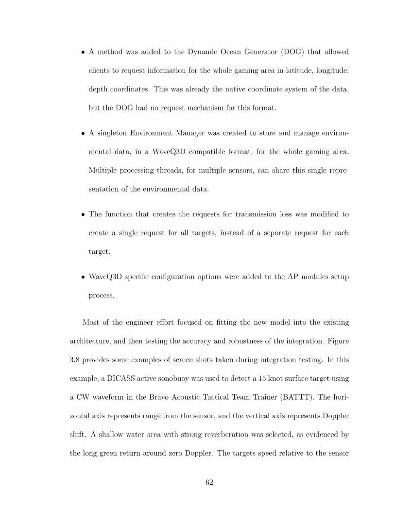
• A method was added to the Dynamic Ocean Generator (DOG) that allowed

clients to request information for the whole gaming area in latitude, longitude,

depth coordinates. This was already the native coordinate system of the data,

but the DOG had no request mechanism for this format.

• A singleton Environment Manager was created to store and manage environ-

mental data, in a WaveQ3D compatible format, for the whole gaming area.

Multiple processing threads, for multiple sensors, can share this single repre-

sentation of the environmental data.

• The function that creates the requests for transmission loss was modified to

create a single request for all targets, instead of a separate request for each

target.

• WaveQ3D specific configuration options were added to the AP modules setup

process.

Most of the engineer effort focused on fitting the new model into the existing

architecture, and then testing the accuracy and robustness of the integration. Figure

3.8 provides some examples of screen shots taken during integration testing. In this

example, a DICASS active sonobuoy was used to detect a 15 knot surface target using

a CW waveform in the Bravo Acoustic Tactical Team Trainer (BATTT). The hori-

zontal axis represents range from the sensor, and the vertical axis represents Doppler

shift. A shallow water area with strong reverberation was selected, as evidenced by

the long green return around zero Doppler. The targets speed relative to the sensor

62

caused the target echo to be Doppler shifted from the reverberation, and this appears

as the return highlighted by the plot annotations.

Figure 3.8: Comparison of sonar displays on BATTT

To quantify the differences between the two models, difference in the transmission

loss, travel time, and source/receiver angles of each eigenray were measured and ana-

lyzed.8 Table 3.1 presents the differences between the WaveQ3D and FeyRay models,

for the scenario illustrated in Figure 3.8. Our analysis indicates that differences be-

tween the two models were primarily due to differences in the sound velocity profiles

in the 2-D and 3-D environments.

63

Table 3.1: Differences in WaveQ3D eigenrays, relative to FeyRay.

Path Time Launch Arrival TL

Direct 0.2 ms 0.104 0.09 0.44 dB

Surface 0.0 ms 0.245 0.450 0.65 dB

Bottom 0.1 ms 0.646 3.192 0.53 dB

3.6 Conclusions

The LVCMS/ASW VAST suite of training systems increase the opportunities for

sonar technicians and commanders, from the Air Tactical Officers all the up to the

Theater ASW Commander, to practice playing together as a team. A new acoustic

transmission model, WaveQ3D, has been developed to improve the scope and com-

plexity of this training without sacrificing fidelity and without increasing hardware

costs or footprint. Future work includes:

• Development of a reverberation model based on WaveQ3D,

• Replacing the legacy model in all LVCMS/ASW VAST signal processing mod-

ules,

• Continuing to support accuracy testing, and

• Improving other sonar training systems using this technology.

The WaveQ3D model is an open-source product distributed as part of the Under

Sea Modeling Library (USML), in accordance with the BSD 2-Clause License. Official

64

releases are posted to the Ocean Acoustics Library,1 sponsored by the U.S. Office of

Naval Research. Third parties are also free to contribute to the development of this

model by forking the Git repository.2

3.7 Acknowledgments

This model was developed as part of Sean Reilly’s PhD studies at the Ocean Engineer-

ing Department of the University of Rhode Island, under the direction of Dr. Gopu

Potty and Dr. James Miller. Testing and productization of this model were funded

by Michael Vaccaro as part of the High Fidelity Active Sonar Training (HiFAST)

Project at the U.S. Office of Naval Research.

3.8 About the Authors

Mr. Sean M. Reilly is a Ph.D. student at the University of Rhode Island and serves

as the Senior System Architect for the Air Force Modeling and Simulation Training

Toolkit (AFMSTT) at The AEgis Technologies Group. He received his M.S. and

B.S. in Physics at the University of Connecticut, with a specialty in computational

Physics. Sean was previously the System Architect for the Navy Continuous Training

Environment (NCTE), as well as working on the High Fidelity Active Sonar Train-

ing (HiFAST) project at Office of Naval Research to develop a new 3D underwater

acoustic propagation loss model for real-time, active sonar, simulation/stimulation

1http://oalib.hlsresearch.com/Rays/USML/usml frontpage2https://github.com/campreilly/UnderSeaModelingLibrary

65

systems in littoral environments.

Mr. Jonathan Glass is a Program Manager of the Live Virtual Constructive

Modeling and Simulation (LVCMS) training suite at the Naval Air Warfare Center

Training Systems Division in Orlando, FL. He has over 20 years of experience as a

Sonar Modeling and Acoustic simulation environments.

66

Manuscript 4

Evaluating accuracy limits of Gaussian ray bundling model in the deep sound

channel

by

Sean M. Reilly and Gopu R. Potty

Ocean Engineering Department, University of Rhode Island

Narragansett, Rhode Island 02882

Planning to submit to Proceedings of Meetings on Acoustics (POMA)

67

4.1 Abstract

Acoustic tomography uses propagation models to predict the multi-path arrival struc-

ture of one-way transmissions received from a distant source. Tomographic inversion

repeatedly perturbs the ocean sound speed and re-computes the arrival structure until

only trivial differences remain between the measured and modeled results. WaveQ3D

is a new 3D Gaussian ray bundling model that is designed to reduce the computation

burden of propagation loss calculations. This feature may have significant benefit in

tomographic inversion, where thousands of modeling runs may be required to converge

on a solution. However, speed is only a benefit if the model accurately predict the

multi-path arrival structure for a given profile. This paper investigates WaveQ3D’s

ability to predict the multi-path arrival structure for the Munk profile, an idealized

representation of deep sound channel conditions in the North Pacific.

4.2 Introduction

Acoustic tomography uses propagation models to predict the multi-path arrival struc-

ture of one-way transmissions received from a distant source.40 Tomographic inversion

repeatedly perturbs the ocean sound speed and re-computes the arrival structure until

only trivial differences remain between the measured and modeled results. WaveQ3D

is a new 3D Gaussian ray bundling model that is designed to reduce the computation

burden of propagation loss calculations. This feature may have significant benefit in

tomographic inversion, where thousands of modeling runs may be required to converge

68

on a solution. However, speed is only a benefit if the model accurately predict the

multi-path arrival structure for a given profile. This paper investigates WaveQ3D’s

ability to predict the multi-path arrival structure for the Munk profile, an idealized

representation of deep sound channel conditions in the North Pacific.28

z′ = 2z − z1B

(4.1)

c(ρ) = c1

[1 + ε

(z′ − 1 + e−z

′)]

(4.2)

where z′ is the normalized depth (positive is down), z1 is the depth of the deep sound

channel axis (1300 meters below ocean surface), B is a depth scaling factor (1300

meters), c1 is the sound speed on the deep sound channel axis (1500 m/s), and ε is a

profile scaling factor (7.37x10-3).

4.3 Benchmark solution for Snell’s Law in spheri-

cal media

WaveQ3D computes propagation on a spherical section of the Earth using geodetic

coordinates: latitude, longitude, and altitude. This approach speeds up 3D applica-

tions by using environmental parameters and their derivatives directly in the latitude,

longitude, and depth directions without reducing the problem to a series of Nx2D

Cartesian projections. Snell’s Law for spherical media (Eq. (4.3)) allows us to build

an benchmark propagation solution that is also based on a spherical Earth.10

m =ρ cos η

c(ρ)= constant (4.3)

69

Figure 4.1: (a) Munk profile, an idealized representation of deep sound channel condi-

tions in the North Pacific. (left panel) Ray paths trapped in the deep sound channel.

dθ

dρ=

1

ρ

cos η(ρ)

sin η(ρ)(4.4)

θ =

∫ ρt

ρs

mc(ρ)

ρ√ρ2 − (mc(ρ))2

dρ (4.5)

τ =

∫ ρt

ρs

ρ

c(ρ)√ρ2 − (mc(ρ))2

dρ (4.6)

where η is the depression/elevation angle along the ray path; m is the ray parameter

for spherical media (constant for each launch angle), τ is the travel time along the ray

path; ρs is the radial coordinate for the source depth; and ρt is the radial coordinate

70

Figure 4.2: (a) Munk profile (b) eigenrays to a target at 200 km, computing usingSnell’s Law for spherical media, legend indicates launch angle.

for the target depth. Although these integrals only apply between the source and

the first vertex or reflection, paths out to any range can be constructed by repeating

this process after the vertex or reflection. In Figure 4.1, our spherical coordinates

benchmark solution for ray paths in a deep sound channel are computed by applying

Eq. (4.5) to the Munk profile.28 In this implementation, integrals are evaluated dis-

creetly using the MATLABTMquadgk implementation of an adaptive Gauss-Kronrod

quadrature.39

The eigenrays are the discreet set of paths that connect the source to a target

at the same depth. To find eigenrays for the benchmark solution, we break the each

71

Table 4.1: Eigenrays to a target at 200 km, computing using Snell’s Law in sphericalmedia.

ID Launch Angle (deg) Travel Time (sec)

1 13.2195 132.8836

2 -8.1769 133.2306

3 -5.2455 133.2876

4 5.2455 133.2876

5 1.7881 133.2995

propagation path into a series of source depth crossings, and calculate the range at

which each crossing occurs. After an even number of crossings, paths that left the

source traveling up will arrive at their target from below. At the end of each cycle, the

ranges for each path increase monotonically as a function of increasing launch angle.

An eigenray is present when these ranges span the target location. Interpolation

allows us to invert range as a function of launch angle into launch angle at the target

range. The same process is used for Eq. 4.6, the travel time integral . To find all

eigenrays, the process is repeated for odd numbers of crossings, and paths that leave

the source traveling down. Figure 4.2 and Table 4.1 illustrate the eigenrays computed

using this technique. Note that in Figure 4.2, distances are converted to range along

the surface of the earth by multiplying ∆θ by the standard radius of the FAI Sphere

(6371.0 km).16

72

4.4 Equivalent benchmark solution in Cartesian

coordinates

To evaluate the impact of numerical error in the discreet evaluation of Eqs. (4.5) and

(4.6), an equivalent benchmark solution is also computed in Cartesian coordinates.

The Earth Flattening Transform26 allows acoustic models that are based on depth and

range to incorporate Earth curvature effects into their calculations. To understand

the Earth Flattening Transformation, we start by looking at propagation on a range-

independent spherical Earth, an environment where environmental parameters doe

not depend on latitude or longitude. In this environment, propagation can be modeled

using the 2D Helmholtz equation in cylindrical coordinates.

∂2ψ

∂ρ2+

1

ρ2∂2ψ

∂θ2+

(2πf

c(ρ)

)2

ψ = 0 (4.7)

where f is frequency of signal; c(ρ) is speed of sound as a function of depth in this

coordinate system. We define an equivalent flat Earth using a change of variables

(x, z).

x = R θ (4.8)

z = R− ρ (4.9)

c′(z) = c(R− z) (4.10)

73

where R is radius of the earth; x is range as change in distance along the surface of the

earth; z is depth below the ocean surface (mean sea level); and c′(z) is speed of sound

as a function of depth in this coordinate system. To model acoustic propagation in

the (x, z) system, we use another change of variables (x, u) to transform Eq. 4.7 into

a Cartesian form.

ρ = Re−uR (4.11)

c′(ρ) =ρ

Rc(u) (4.12)

dρ = −e−uRdu = − ρ

Rdu (4.13)

dθ =1

Rdx (4.14)(

−Rρ

)2∂2ψ

∂u2+

(R

ρ

)2∂2ψ

∂x2+

(R

ρ

2πf

c′(u)

)2

ψ = 0 (4.15)

∂2ψ

∂x2+∂2ψ

∂u2+

(2πf

c′(u)

)2

ψ = 0 (4.16)

where ρ is depth non-linear function of ρ; c′(u) is speed of sound as a function of depth

in this coordinate system. The relationship between the (x, z) and (x, u) coordinate

systems is given by

u = −R ln(

1− z

R

)(4.17)

c′(u) = c′(z)/(

1− z

R

)(4.18)

The relationship between z and u is often approximated.

u = −R[(− zR

)− 1

2

(− zR

)2+

1

3

(− zR

)3− ...

](4.19)

u1 ≡ z (4.20)

74

u2 ≡ z[1 +

z

2R

](4.21)

where u1 is the first order approximation; and u2 is the second order approximation.

The analysis solution in (x, u) terms is implemented using Snell’s Law in Cartesian

coordinates.

a =cos η(u)

c′(u)= constant (4.22)

dx

du=

cos η(u)

sin η(u)(4.23)

x =

∫ ut

us

ac′(u)√1− (ac′(u))2

du (4.24)

t =

∫ ut

us

1

c′(u)√

1− (ac′(u))2du (4.25)

where η(u) is the depression/elevation angle along the ray path; a is the ray parameter

in Cartesian coordinates (constant for each launch angle); t is the travel time in

Cartesian coordinates; us is the source depth; and ut is the target depth. In theory,

there should be no difference between the results computed using Eqns. (4.5) to (4.6)

and those computed using Eqns. (4.24) to (4.25).

Table 4.2: Largest errors for each versions of the Earth Flattening Transform.

ID Range Error (m) Time Error (msec)

no transform +690.1 +464.4

1st order -28.72 -18.92

2nd order +0.2538 +0.1637

no approx +0.2706 +0.1747

Figures 4.3 and 4.4 illustrates the difference between the Cartesian and spherical

benchmark solutions to Snell’s Law, using different versions of the Earth Flattening

75

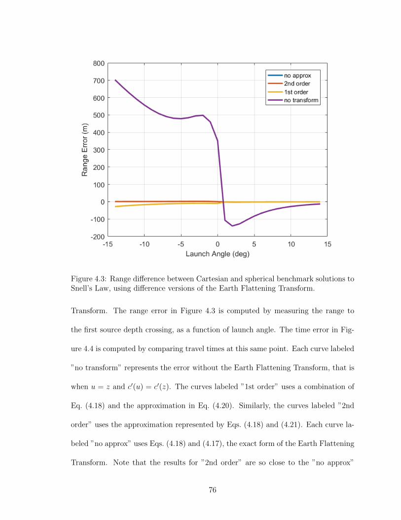
Figure 4.3: Range difference between Cartesian and spherical benchmark solutions toSnell’s Law, using difference versions of the Earth Flattening Transform.

Transform. The range error in Figure 4.3 is computed by measuring the range to

the first source depth crossing, as a function of launch angle. The time error in Fig-

ure 4.4 is computed by comparing travel times at this same point. Each curve labeled

”no transform” represents the error without the Earth Flattening Transform, that is

when u = z and c′(u) = c′(z). The curves labeled ”1st order” uses a combination of

Eq. (4.18) and the approximation in Eq. (4.20). Similarly, the curves labeled ”2nd

order” uses the approximation represented by Eqs. (4.18) and (4.21). Each curve la-

beled ”no approx” uses Eqs. (4.18) and (4.17), the exact form of the Earth Flattening

Transform. Note that the results for ”2nd order” are so close to the ”no approx”

76

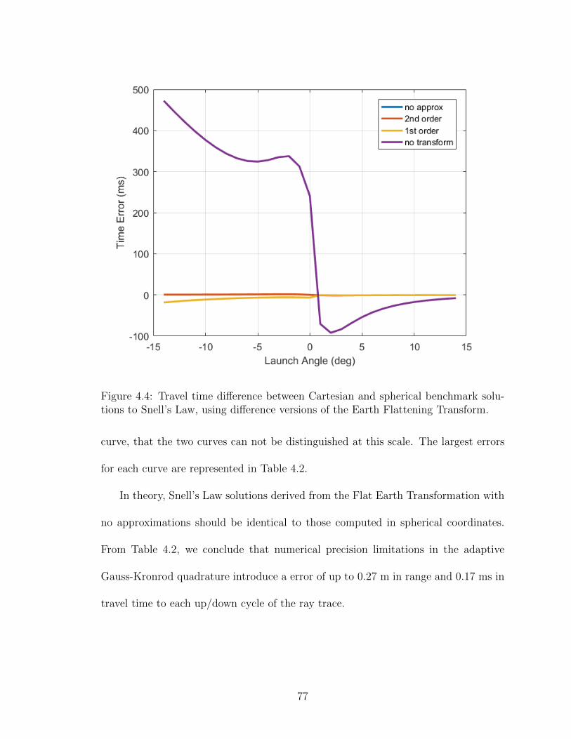
Figure 4.4: Travel time difference between Cartesian and spherical benchmark solu-tions to Snell’s Law, using difference versions of the Earth Flattening Transform.

curve, that the two curves can not be distinguished at this scale. The largest errors

for each curve are represented in Table 4.2.

In theory, Snell’s Law solutions derived from the Flat Earth Transformation with

no approximations should be identical to those computed in spherical coordinates.

From Table 4.2, we conclude that numerical precision limitations in the adaptive

Gauss-Kronrod quadrature introduce a error of up to 0.27 m in range and 0.17 ms in

travel time to each up/down cycle of the ray trace.

77

4.5 WaveQ3D accuracy

To evaluate the accuracy limits of WaveQ3D in this application, we propagated a

wavefront to a target 200 km north of the source. To mimic the conditions from our

benchmark solutions, we limited the ray fan to ±14o in the vertical and ±0.2o in the

horizontal. Spacing between rays was set to 0.1o in both directions. The wavefronts

were propagated in time with a step size that varied from 25 to 100 ms.

Figure 4.5: Range difference between WaveQ3D and Snell’s Law in spherical media,for 25 ms time step, after 4 complete cycles. Includes comparison to Flat EarthTransform with no approximations.

Figures 4.5 and 4.4 illustrates the difference between the WaveQ3D results with

78

Figure 4.6: Travel time difference between WaveQ3D and Snell’s Law in sphericalmedia, for 25 ms time step. Includes comparison to Flat Earth Transform with noapproximations.

Table 4.3: Largest errors for each step size in WaveQ3D

Step (ms) Range Error (m) Time Error (msec) Exec Speed (s)

100 -26.48 -0.9723 0.5

50 -3.315 -0.1394 0.9

25 -0.4146 -0.0385 1.8

flat earth +1.135 -0.0239 n/a

a time step of 10 ms and spherical benchmark solutions to Snell’s Law. To estimate

range error in the vicinity of the 200 km target, Figure 4.5 changes the definition

79

or range error to be the difference after each solution completes 4 cycles. The time

error is computed as the difference in eigenray travel times at the 200 km target.

These figures includes a comparison to Flat Earth Transform equivalent with no

approximations to illustrate the scale of these error relative to numerical precision

limitations in the adaptive Gauss-Kronrod quadrature.

The largest errors for each time step setting are represented in Table 4.3. In

addition to illustrating the dependence of errors on time step size, this table also

includes the execution time needed to compute WaveQ3D eigenray results for this

scenario on a single core of a Dell Latitude E6540 laptop with an Intel(R) i7-4810MQ

CPU @ 2.80 GHz. Execution speed information is provided for acoustic tomography

researchers who may be interested in the relationship between accuracy and compu-

tational efficiency for inversion applications.

4.6 Conclusions

For a target at 200 km, the differences between WaveQ3D and the benchmark solu-

tions for Snell’s law in spherical media less than 1.6x10−4% in range and 2.9x10−5% in

travel time, for a time step of 25 ms. However, these differences are nearly identical

to the errors introduced by numerical precision limitations in the adaptive Gauss-

Kronrod quadrature used in the benchmark solution. For a time step of 25 ms, there

appears to be no significant difference between WaveQ3D accuracy and that of the

benchmark.

Acknowledgments

80

The authors greatly appreciate the help that Dr. John Colosi (Naval Post Grad-

uate School), Dr. Brian Dushaw (Applies Physics Laboratory/University of Wash-

ington), and Dr. Timothy Duda (Woods Hole Oceanographic Institution) provided

on the proper application of the Flat Earth Transform. Special thanks to Dr. Colosi

who also provided the derivation of the Flat Earth Transform used in this paper from

his personal notes.

81

Appendix A

Verification Tests for Hybrid Gaussian Beams in Spherical/Time Coordinates

by

Sean M. Reilly and Gopu R. Potty

Ocean Engineering Department, University of Rhode Island

Narragansett, Rhode Island 02882

Report delivered to High Frequency Active Sonar Training (HiFAST) Project

at the U.S. Office of Naval Research (ONR), May 2012

82

A.1 Abstract

The theory paper defined a new undersea acoustic propagation loss model that is

specifically designed to support real-time, sonar simulation/stimulation systems, in

littoral environments, at active sonar frequencies. This paper seeks to verify the

model’s implementation by comparing the modeled results to analytic solutions.

A.2 Introduction

The theory paper38 defined the theory for a new undersea acoustic propagation loss

model that is specifically designed to support real-time, sonar simulation/stimulation

systems, in littoral environments, at active sonar frequencies. The WaveQ3D model

implements this theory using a circular queue of time domain wavefronts, in a fully 3-D

ocean environment, with a computationally-efficient form of C++ vector processing.44

This follow-up paper analyzes the capabilities and limitations of this implementation.

The Capability Maturity Model Integration (CMMI)11 separates testing needed for

such an effort into two phases:

• Verification testing ensures that selected work products meet their specified

requirements. For this analysis, the WaveQ3D model is decomposed into its

component parts (such as ray tracing, reflection, eigenray finding, and propaga-

tion loss), and the results from each parts are compared to analytic solutions.

• Validation testing demonstrates that a product or product component fulfills

its intended use when placed in its intended environment. For the WaveQ3D

83

model, this will consist of comparisons to real-world results in a subsequent

paper.

Decomposing the testing in this way is designed to ensure that any conclusions drawn

from the modeled results rest on a firm foundation of understanding.

A.3 Ray Tracing Tests

The ray paths in this model use a third order Adams-Bashforth (AB3) marching

solution49 to create a circular queue of time domain wavefronts. The evolution of the

wavefront shape, as it passed through the 3-D ocean environment, is defined by the

following equations.

dr

dt= c2α , (A.1)

dθ

dt=c2β

r, (A.2)

dφ

dt=

c2γ

r sin θ, (A.3)

dα

dt= −1

c

dc

dr+c2

r

(β2 + γ2

), (A.4)

dβ

dt= − 1

c r

dc

dθ− c2

r

(αβ + γ2cotθ

). (A.5)

dγ

dt= − 1

c r sin θ

dc

dφ− c2γ

r(α + β cot θ) , (A.6)

where c is the speed of sound as a function of location; t is the travel time; (r, θ, φ)

are the spherical earth coordinates of the modeled ray path as a function of time;

and (α, β, γ) are the spherical earth coordinates of the normalized ray direction as a

function of time. The tests discussed in this section analyze the accuracy of Eqs. (A.1)

through (A.6) in scenarios where the rays do not encounter any boundaries.

84

A.3.1 Comparisons to “flat earth” benchmarks

Because WaveQ3D is one of the few models to use non-Cartesian coordinate system,

comparisons to other work often require translation before differences can be ana-

lyzed. This section analyzes the accuracy of the translation between spherical and

Cartesian coordinate models. Cartesian coordinate propagation models frequently

use a modified index of refraction33 to incorporate earth curvature effects into their

calculations.

n′(r) =r

R

n(r)

n(R), (A.7)

c′(z) =c(z)

1− z/R, (A.8)

where R is the radius of earth’s curvature in this area of operations; r is the radial

distance from the center of curvature (positive is up); z = R − r is the below the

ocean surface (positive is down); n(z), n′(z) are the original and modified index of

refraction, and c(z), c′(z) are the original and modified speed of sound. When a testing

benchmark is specified in Cartesian coordinate, the inverse of this process must be

implemented to create an equivalent environment in spherical earth coordinates.

c′(r) =r

Rc(r) , (A.9)

where c(r) is the benchmark’s original c(z) sound speed converted to a function of r.

The Munk profile28 was used to evaluate the accuracy of testing Cartesian bench-

marks in a model based on spherical earth coordinates. The Munk profile is an

idealized representation of a typical deep sound channel, and it was chosen for its

85

ability to support long range paths without interface reflection.

z′ = 2z − z1B

, (A.10)

c(z) = c1

[1 + ε

(z′ − 1 + e−z

′)]

, (A.11)

where z′ is the normalized depth (positive is down), z1 is the depth of the deep

sound channel axis (1300 meters), B is a depth scaling factor (1300 meters), c1 is the

sound speed on deep sound channel axis (1500 m/s), and ε is the profile scaling factor

(7.37x10-3). The specific Munk profile parameters used in this test were selected to

match Fig. 3.19 in Jensen, Kuperman, et. al.21;36 An example of the ray paths for

this profile are illustrated in Fig. A.1. This figure was created by WaveQ3D with a

100 ms time increment and 1o separated depression/elevation launch angles from -14o

to 14o. Launch angles greater than 14.38o encounter interface reflections.

Munk’s paper28 characterized the analytic solution for ray paths using their cycle

range, the range required to complete one period of upward and downward refraction.

The cycle range is equal for positive and negative launch angles. The cycle range was

used as the metric for this test because it could be cast into identical units in both

spherical and Cartesian coordinates.

To create an analytic equivalent to a typical Cartesian model, Snell’s Law (Eq.

A.12) was integrated numerically, using the MATLABTMquadgk() implementation of

an adaptive Gauss-Kronrod quadrature.39

a =cos η(z)

c(z)= constant , (A.12)

dH

dz=

cos η(z)

sin η(z), (A.13)

86

0 20 40 60 80 100 120 140−5000

−4500

−4000

−3500

−3000

−2500

−2000

−1500

−1000

−500

0

Range (km)

De

pth

(m

)

Figure A.1: Modeled ray paths for the Munk profile.

∆H =

∫ zt

zs

ac(z)√1− (ac(z))2

dz , (A.14)

∆t =

∫ zt

zs

1

c(z)√

1− (ac(z))2dz , (A.15)

where η(z) is the depression/elevation angle along the ray path; a is the ray parameter

(constant for each launch angle); H is the horizontal range; t is the travel time; zs

is the source depth; and zt is the target depth. Although these integrals only apply

between the source and the first vertex or reflection, paths out to any range can be

constructed by repeating this process after the vertex or reflection.

To create equivalent conditions for a model based on spherical earth coordinates,

87

we modified the original sound speed using Eq. (A.9), and then performed a similar

integration in spherical coordinates. Snell’s law in spherical media includes an extra

factor of r that is not present in the Cartesian coordinates.10 The slope of the ray

path also includes an extra factor ofr in spherical coordinates.

p =r cos η(r)

c(r)= constant (A.16)

rdθ

dr=

cos η(r)

sin η(r)(A.17)

∆θ =

∫ rt

rs

pc(r)

r√r2 − (pc(r))2

dr (A.18)

∆t =

∫ rt

rs

r

c(r)√r2 − (pc(r))2

dr (A.19)

where η(r) is the depression/elevation angle along the ray path; p is the ray parameter

for spherical media (constant for each launch angle), ∆θ is the horizontal range in

solid angle units; rs is the radial coordinate for the source depth; and rt is the radial

coordinate for the target depth.

The difference in the cycle ranges computed using these two analytic solutions is

shown in A.2. The results were computed for two complete periods, with launch angles

from 0o to 14o, as a function of the spherical coordinates cycle range solution. The

0o launch angle has difference of -5.14 meters at a range of 96.16 km. The 14o launch

angle has a has difference of -38.34 meters at range of 129.95 km. The intermediate

angles have monotonically increasing values between those two extremes.

Since both solutions are analytic, we conclude that difference must be a fun-

damental property of ray paths computations in the two coordinate systems. It is

equally valid to attribute these results to

88

95 100 105 110 115 120 125 130−40

−35

−30

−25

−20

−15

−10

−5

Range (km)

Ra

ng

e E

rro

r (m

)

Figure A.2: earth-flattening accuracy for the Munk profile.

• Errors created by a spherical model working with a Cartesian environment, or

• Errors created by a Cartesian model working with a spherical environment.

The second case is more interesting for this study, because it represents a widely ac-

cepted (but seldom mentioned) lower limit on ray path range accuracy, approximately

0.03% of the total range.

89

A.3.2 Ray path accuracy in a deep sound channel

In this test, the refraction accuracy of the WaveQ3D model was computed for a

“flat earth” Munk profile defined in spherical coordinates by combining Eqs. (A.10)

and (A.11) with Eq. (A.9). Fig. A.3 illustrates the difference between individual

WaveQ3D rays and the spherical analytic solution defined by Eqs. (A.16) through

(A.18). Cycle ranges were computed for both the first and second period of the

SOFAR cycle. Because both solutions were computed in spherical coordinates, using

the same sounds speed profile, these error can not be attributed to the use of a

modified index of refraction.

With a 100 ms step size, the WaveQ3D result deviates from the analytic solution

by a maximum of -8.62 meters at cycle range of 129.95 km (0.007% error). However,

50 out of 58 samples (86%) exhibited errors less than ± 2 meters (0.002% error). Ray

paths that were initially launched toward the surface, where the sound speed gradient

is highest, had consistently larger errors than paths that were launched down. The

fact that these errors were all significantly less than those of associated with the earth

curvature correction (Fig. A.2) suggests that WaveQ3D model’s cycle range estimate

meets or exceeds the accuracy of Cartesian models used on a spherical earth.

To estimate the impact of WaveQ3D options on this result, the maximum error

was also computed as a function of time step size. The circles in Fig. A.4 represent

maximum errors, across launch angles, for time steps of 25, 50, 100, 150, 200, 250, 300,

350, and 400 ms. The connecting lines smoothly interpolate between these discreet

values. From this, we conclude that the accuracy of WaveQ3D cycle range estimates is

90

0 20 40 60 80 100 120 140−10

−8

−6

−4

−2

0

2

Range (km)

Ra

ng

e E

rro

r (m

)

Launched Up

Launched Down

Figure A.3: WaveQ3D errors for the Munk profile.

slightly weaker than a power law; a doubling of the time step decreased the accuracy

by approximately a factor of 10. Step sizes as large as 150 yielded results that were at

least as accurate as errors associated with the modified index of refraction. Given that

some environments may have stronger gradients than the Munk profile, we conclude

that a 100 ms step size should be adequate for most long range applications.

91

0 50 100 150 200 250 300 350 400 45010

−1

100

101

102

103

Time Step (msec)

Ra

ng

e E

rro

r (m

)

Figure A.4: Path accuracy sensitivity to step size for the Munk profile.

A.3.3 Ray path accuracy in an extreme downward refraction

environment

In this test, the refraction accuracy of the WaveQ3D model was computed for the

extreme n2 linear test case developed by Pedersen and Gordon.32

c(z) =c0√

1 + 2g0c0z

(A.20)

where c0 is the sound speed at the ocean surface (1550 m/s); g0 is the sound speed

gradient at at the ocean surface (1.2 s-1). At shallow depths, this profile matches

92

observed conditions from the Pacific, in an area of extreme velocity gradient. But at

depths greater than about 60 meters, it predicts theoretically useful, but physically

unrealistic sound speeds. This profile was selected for this study because of its wide

use by other authors in the testing of Gaussian beam model behavior at the edge

of a shadow zone.34;45 (Note that the specific values for this profile parameters were

selected to match the MKS representation of Eq. 3.47 in Jensen, Kuperman, et. al.21

instead of the English units used in the original Pedersen and Gordon paper.)

0 0.5 1 1.5 2 2.5 3 3.5−1200

−1000

−800

−600

−400

−200

0

Range (km)

Depth

(m

)

Figure A.5: Modeled ray paths for the Pedersen/Gordon profile.

The ray paths to be tested for this profile are illustrated in Fig. A.5. This figure

was created by WaveQ3D with a 100 ms time increment and 1o separated depres-

93

sion/elevation launch angles from 20o to 50o. A “flat earth” adjustment was applied

to Eqn. A.20 to allow these results to be similar to those computed in Cartesian coor-

dinates. Launch angles greater than 51.21o encounter interface reflections. The rays

launched at angles between 44o and 50o travel through a caustic and cross the direct

path rays. Because the ray paths were not periodic, we redefined the cycle range as

the horizontal range needed to travel up to the first vertex and back to the source

depth. Figure A.6 illustrates the difference between individual WaveQ3D rays and

the spherical analytic solution defined by Eqs. (A.16) through (A.18). The WaveQ3D

model had a maximum error of 1.3 m at cycle range of 2595.1 m (0.05% error), but

there appeared to be a slight bias. We discovered that many of the launch angles had

cycle range errors right around -0.5 m.

The sensitivity of these results to time step size is illustrated in Fig. A.7. The

150 ms step size had errors of about 2 meters. Errors for smaller time steps approached

zero as expected. Larger time steps increase as a power law until the step size was

larger than 350 ms, where the error quickly grew to hundreds of meters. This sudden

change in error appears to be the result of an inability of model to properly sample

the sound velocity profile field at the larger step sizes. From this, we conclude that

our earlier 100 ms time step recommendation continues to be valid for this case.

A.3.4 Ray path accuracy along great circle routes

In this test, an ocean with a small amount of downward refraction was used to verify

the WaveQ3D model’s ability to propagate rays along great circle routes. Acoustic

94

2 2.5 3 3.5−1

−0.5

0

0.5

1

1.5

Range (km)

Ra

ng

e E

rro

r (m

)

Figure A.6: Path accuracy sensitivity to step size for the Pedersen/Gordon profile.

rays traveling at a constant depth follow these paths because they are the shortest

distance between two points along the earth’s surface. The amount of downward

refraction needed to parallel the earth’s surface was computed by inverting Eq. A.9

c(r) =r

Rc0 . (A.21)

where c0 was set to 1500 m/s.

This test launched four horizontal rays from 45N 45W, at a depth of 1000 meters,

with azimuths of 0o, 30o, 60o, and 90o. The rays propagated for 1000 s (about

1500 km) with a time step of 100 ms. Fig. A.8 illustrates the resulting ray paths as a

function of latitude and longitude. The solid lines represent acoustic ray paths while

95

0 50 100 150 200 250 300 350 400 45010

−2

10−1

100

101

102

103

Time Step (msec)

Ra

ng

e E

rro

r (m

)

Figure A.7: Ray path accuracy as a function of step size for the Pedersen/Gordonprofile.

the dashed lines represent the rhumb line paths, paths that would have been taken if

latitude/longitude were a Cartesian system. The accuracy of the great circle routes

were computed by converting the latitude, longitude, and altitude of each ray back

into a great circle azimuth at the point of origin47

ϕa(t) = arctan

[cosχ(t) sin(φ(0)− φ(t))

cosχ(0) sinχ(t)− sinχ(0) cosχ(t) cos(φ(0)− φ(t))

], (A.22)

where χ(t), φ(t) are latitude and longitude as a function of time; and ϕa(t) is the

analytic solution for the azimuthal launch angle for a target at χ(t), φ(t). The rays

traveled at constant depth with a maximum deviation from ϕa(t) of 2.81x10-10 degrees.

96

−46 −44 −42 −40 −38 −36 −34 −32 −30 −28 −2642

44

46

48

50

52

54

56

58

60

Longitude (deg)

La

tgitu

de

(d

eg

)

Figure A.8: Great circle routes.

This level of accuracy should be more than adequate for most applications.

A.4 Interface Reflection Tests

The WaveQ3D model estimates the partial time step during a 3-D interface collision

using the equation

δt =h r · s

d~r

dt· s

(A.23)

97

where s is the surface normal; r is the unit vector in the radial direction; h is the

incident ray height above bottom; δt is the time step needed to reach the interface;

and drdt

is the radial ray tracing component defined by Eq. (A.1). The direction of the

3–D reflection is computed using

R = I − 2(I · s)s (A.24)

where I is the incident ray path direction; and R is the reflected ray path direction.

The WaveQ3D model also applies a second order Taylor expansion to each component

of the position, normalized direction, and sound speed to improve the accuracy of their

values at the time of collision. The tests discussed in this section analyze the accuracy

of this reflection process in an isovelocity ocean.

A.4.1 Reflection accuracy with a flat bottom

This test constructed a geometry in which the changes in latitude and travel time for

multiple interface bounces could be calculated analytically. The path of a downwardly

steered ray, given a constant bottom depth and latitude change, is illustrated by

Fig. A.9 and the equations

ζs = arcsin

(R2 −R2

b + L2

2RL

), (A.25)

ζb = ζs −∆θ/2 , (A.26)

t = L/c , (A.27)

where R is the radius for the ocean surface; D is the water depth; Rb = R−D is the

radius for the ocean bottom; ∆θ is the latitude change between surface bounces; L

98

Figure A.9: Flat bottom reflection geometry.

is the path length from surface to bottom; ζs is the grazing angle at the surface (also

the ray launch angle); ζb is the grazing angle at bottom; c is the sound speed; and t

is the travel time between the surface and the bottom.

∆θ was set 0.2o and the ocean depth was set to 1000 meters, which caused the

remaining parameters take on the analytic values shown in Table A.1. A single

WaveQ3D ray was launched at a depression/elevation angle of -5.183617057o (down),

and a time step of 100 ms, which produced the path shown in Fig. A.10. After

four complete cycles of bottom and surface reflection, a distance of about 89 km,

the latitude for the point of reflection deviated from the analytic result by less than

3.9x10-7 degrees (about 40 cm). The travel time differed from the analytic result by

99

Table A.1: Flat bottom expected values.

Parameter Analytic Result

c 1500 m/s

D 1000 m

∆θ 0.2o

ζs 5.183617057o

ζb 5.083617057o

L 11,175.841460125 m

t 7.450560973 s

less than 2.9x10-5 s. From this, we conclude that the WaveQ3D reflection process has

an acceptable reflection accuracy when the interfaces are flat.

A.4.2 Reflection accuracy with a sloped bottom

This test looked at the ability of WaveQ3D to predict the direction of reflection from

a bottom that has a 1 degree up-slope in the latitude direction. At each bottom

reflection, the depression/elevation angle of the WaveQ3D ray path should decrease

by 2o, just like the analytic result. Launching a ray at a the same depression/elevation

angle as the last test (-5.183617057o, down) produced the results shown in Fig. A.11.

Note that the time step for this test was set to 1 ms to make it easier to compute

depression/elevation angle just before, and just after, each collision. The maximum

deviation of any of the three bottom reflections from their analytic reflection direction

result was 1x10-5 degrees. From this, we conclude that WaveQ3D produces acceptable

100

45 45.1 45.2 45.3 45.4 45.5 45.6 45.7 45.8 45.9−1000

−900

−800

−700

−600

−500

−400

−300

−200

−100

0

Depth

(m

)

Latitude (deg)

Figure A.10: Flat bottom reflection test results.

reflections for sloped bottoms.

A.4.3 Out-of-plane reflection from gridded bathymetry

ETOPO1 gridded bathymetry15 from the Malta Escarpment was used to qualitatively

test out-of-plane reflection from realistic bathymetry features. Out-of-plane reflection

is a real-world phenomena that can have a significant impact on shallow water exper-

iments.41 To isolate the testing to reflection effects, the speed of sound was fixed at

1500 m/s at all locations. WaveQ3D used a 100 ms step size to compute a single path,

illustrated in Figure A.12. In this figure, bottom bathymetry contours are represented

101

45 45.05 45.1 45.15 45.2 45.25 45.3 45.35 45.4−1000

−900

−800

−700

−600

−500

−400

−300

−200

−100

0

Depth

(m

)

Latitude (deg)

Figure A.11: Analytic slope reflection test results.

as dashed lines. A ray launched from 35:59N 16:00E, at a depth of 10 meters, with a

depression/elevation angle of -20o (down), and an azimuth of 270o traveled along the

path illustrated by the solid black line. The closed circles along this path represent

places where bottom reflections occurred; the open circles represent surface reflec-

tions. The decrease in spacing between the shallow water dots illustrates the type

of depression/elevation angle change (Fig. A.11) expected for sloped bottoms. What

was new in this test was the face that ray paths were reflected into a new azimuthal

direction each time that they interacted with the bottom. These out-of-plane reflec-

tions resulted in a down slope ray path that was offset by more than 21.9 km from

102

the up slope path, after 14 bounces off of the bottom. From this, we conclude that

WaveQ3D results will have a significant contributions from out-of-plane ray paths

whenever there are multiple interactions with complex bottom bathymetry features.

500

500

500

500

1000

1000

1000

1000

1500

1500

1500

1500

1500

2000

2000

2000

2000

2000

2000

2500

2500

2500

2500

2500

3000

3000

3000

3000

3000

35003500

3500

3500

3500

Latitu

de (

deg)

Longitude (deg)15.4 15.5 15.6 15.7 15.8 15.9 16

35.8

35.9

36

36.1

36.2

36.3

36.4

Figure A.12: Reflection on the Malta Escarpment.

A.5 Eigenray and Propagation Loss Tests

The tests discussed in this section compare WaveQ3D’s eigenray and propagation loss

calculation to analytic solutions.

The WaveQ3D eigenray estimation process establishes the relative geometry be-

103

tween rays paths and targets. That geometry then allows the calculation of travel

time (t), source angle (µ), and target angle (ϕ) for each multi-path arrival. WaveQ3D

computes these eigenray products by searching for the offsets which minimize the

squared distance from targets to points on the wavefront. Once the CPA has been

determined, the 3-D offset to the target is computed using

~ρ ≡ (ρ1, ρ2, ρ3) ≡ (δt, δµ, δϕ) , (A.28)

~g ≡ ∂d2

∂~ρ

∣∣CPA

, (A.29)

H ≡ ∂2d2

∂~ρ2∣∣CPA

(A.30)

~ρ = −H−1 ~g . (A.31)

where ~ρ is the offset from CPA in vector form; d2 is the squared distance from each

point on the wavefront to the target; ~g is the gradient of squared distance, evaluated

at CPA (3 elements), and H is the Hessian matrix of squared distance, evaluated at

CPA (3x3).

The propagation loss at the target location is a summation of contributions from

the rays that surround the eigenray target. To create a 3-D acoustic field across the

wavefront, WaveQ3D uses independent Gaussian beams in the µ and ϕ directions and

ignores the cross terms.

G(~rp) =

(j+J∑

j′=j−J

gj′(~rp)

)(k+K∑

k′=k−K

gk′(~rp)

), (A.32)

gj′(~rp) =(µj′+1 − µj′)√

2πw2j′

exp

(−d2j′

2w2j′

), (A.33)

gk′(~rp) =(sin(µj′+1)− sin(µj′)) (ϕk′+1 − ϕk′)√

2πw2k′

exp

(− d2k′

2w2k′

), (A.34)

104

where G(~rp) is the total Gaussian beam intensity at the eigenray target; (j, k) are the

index numbers of wavefront cell containing the eigenray target; gj′ are the Gaussian

beam contributions along depression/elevation direction; gk′ are the Gaussian beam

contributions along the azimuthal direction; 2J+1 are the number of significant beams

in the depression/elevation direction; and 2K+1 are the number of significant beams

in the azimuthal direction; wj and wk are the half-widths of the Gaussian beam in

the µ and ϕ directions; and d2j and d2k are the distance in the µ and ϕ directions from

the Gaussian beam center to the eigenray target. The WaveQ3D implementation

divides the wavefront into ray families based on the number of surface reflections,

bottom reflections, and caustic encounters. Within each ray family, propagation loss

contributions are added across the wavefront until an edge is hit or the accumulated

loss result changes by less than 0.01 dB.

WaveQ3D treats the beam width calculation as a convolution between Weinberg’s

frequency dependent “minimum width” term45 and a second Gaussian that represents

the spatial spreading created by the sampling of the wavefront.

(w′j,k(f))2 = (2wj,k)2 + (2πλ)2 . (A.35)

where λ is the wavelength of the signal being modeled; wj,k is the cell width of beam

j or k, and w′j,k(f) is the adjusted width of beam j or k. The factor of 2 in the wj,k

term creates a minimum overlap of 50% between neighboring beams. Normalizing

Eqs. (A.33) and (A.34) by the combined effect of both spreading sources conserves

energy across the wavefront.

105

A.5.1 Eigenray accuracy for a simple geometry

This test constructs a short range geometry in which travel time, source angle, and

target angle can be computed analytically for direct path, surface reflected, and bot-

tom reflected paths on a spherical earth. The geometry for this test is illustrated in

Fig. A.13.

Figure A.13: Flat bottom eigenray test geometry.

r = R− d , (A.36)

L1 = 2rsin(∆θ/2) , (A.37)

µ1 = 90o − arccos(L1

2r

), (A.38)

L2 = 2√

(L1/2)2 + [R− r cos(∆θ/2)]2 , (A.39)

106

µ2 = 90o − arccos(

d

L2/2

), (A.40)

L3 = 2√

(L1/2)2 + [r cos(∆θ/2)− (R−D)]2 , (A.41)

µ3 = µ1 + arccos

(L1/2

L3/2

), (A.42)

tn = Ln/c , (A.43)

where c is the sound speed; D is the water depth; d is both the source and target

depth; r is the distance of the source/target from the center of curvature; L1, L2, L3

are the path lengths for the direct, surface reflected, and bottom reflected paths;

t1, t2, t3 are the travel times; and µ1, µ2, µ3 are the source/target depression/elevation

angles.

WaveQ3D was tested using an ocean depth of 3000 m, a ∆θ value of 0.02o, and

the source/target depth of 1000 m. Eqs. (A.36) through (A.43) were then used to

compute the values shown in Table A.2.

WaveQ3D eigenrays were calculated using a ray fan with depression/elevation

angles from -60o to +60o, azimuth angles from -4o to +4o, angle spacings of 1o in

both directions, and a time step of 100 ms. This geometry was specifically designed

to stress the model by forcing it to extrapolate the bottom bounce path from a

location outside of the ray fan. The other two paths are firmly inside of the ray fan.

For the direct path, the maximum difference between the modeled times/angles

and their analytic counterparts were 2.2x10-5 ms and 1.1x10-4 degrees. These values

represented eigenray accuracy limitations purely derived from Eqs. (A.28) through

(A.31). The equivalent measurements for the surface reflected path yielded differences

of 2.2x10-3 ms and 4.8x10-3 degrees. The reduced accuracy of the surface reflected

107

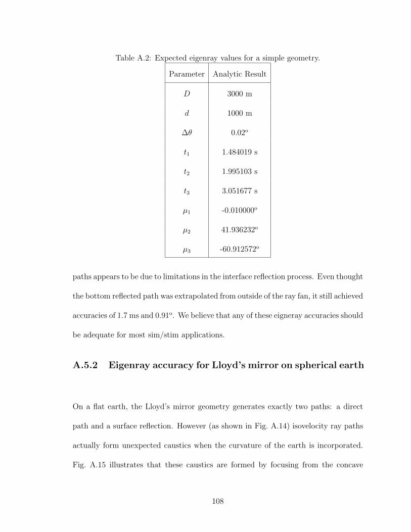
Table A.2: Expected eigenray values for a simple geometry.

Parameter Analytic Result

D 3000 m

d 1000 m

∆θ 0.02o

t1 1.484019 s

t2 1.995103 s

t3 3.051677 s

µ1 -0.010000o

µ2 41.936232o

µ3 -60.912572o

paths appears to be due to limitations in the interface reflection process. Even thought

the bottom reflected path was extrapolated from outside of the ray fan, it still achieved

accuracies of 1.7 ms and 0.91o. We believe that any of these eigneray accuracies should

be adequate for most sim/stim applications.

A.5.2 Eigenray accuracy for Lloyd’s mirror on spherical earth

On a flat earth, the Lloyd’s mirror geometry generates exactly two paths: a direct

path and a surface reflection. However (as shown in Fig. A.14) isovelocity ray paths

actually form unexpected caustics when the curvature of the earth is incorporated.

Fig. A.15 illustrates that these caustics are formed by focusing from the concave

108

surface of the earth. Incorporating these effects into our eigneray tests is important

because of WaveQ3D’s use of spherical earth coordinates.

0 0.2 0.4 0.6 0.8 1 1.2 1.4 1.6−1200

−1000

−800

−600

−400

−200

0

Latitude Change (deg)

Depth

(m

)

Figure A.14: Isovelocity paths in spherical coordinates.

Fig. A.16 defines the geometry used to compute an analytic eigenray solution. In

this figure, d1, d2 are the source and target depths; r1, r2 are the source and target

distance from the center of curvature; ∆θ is the latitude change from source to target;

∆θ1 is the latitude change from the source to the point of reflection; ∆θ2 = ∆θ−∆θ1

is the latitude change from the reflection point to the target; β is the reflection angle

relative to the normal; a is the length of the direct path; and b1 + b2 is the length of

the surface reflected path.

109

0 20 40 60 80 100 120 140 160−2000

−1800

−1600

−1400

−1200

−1000

−800

−600

−400

−200

0

Range (km)

De

pth

(m

)

Figure A.15: Isovelocity paths in Cartesian coordinates.

The analytic solutions for the surface reflected path requires finding values of ∆θ1

which solve the transcendental equation (derived in the Section A.6.1)

r1sin(∆θ1)− r2sin(∆θ −∆θ1) +r1r2R

sin(∆θ − 2∆θ1) = 0 . (A.44)

Once the roots of Eq. (A.44) are known, the analytic solution for surface reflected

eigenrays can be computed using

b21 = R2 + r21 − 2Rr1 cos(∆θ1) , (A.45)

b22 = R2 + r22 − 2Rr2 cos(∆θ2) , (A.46)

ts =b1 + b2c0

, (A.47)

110

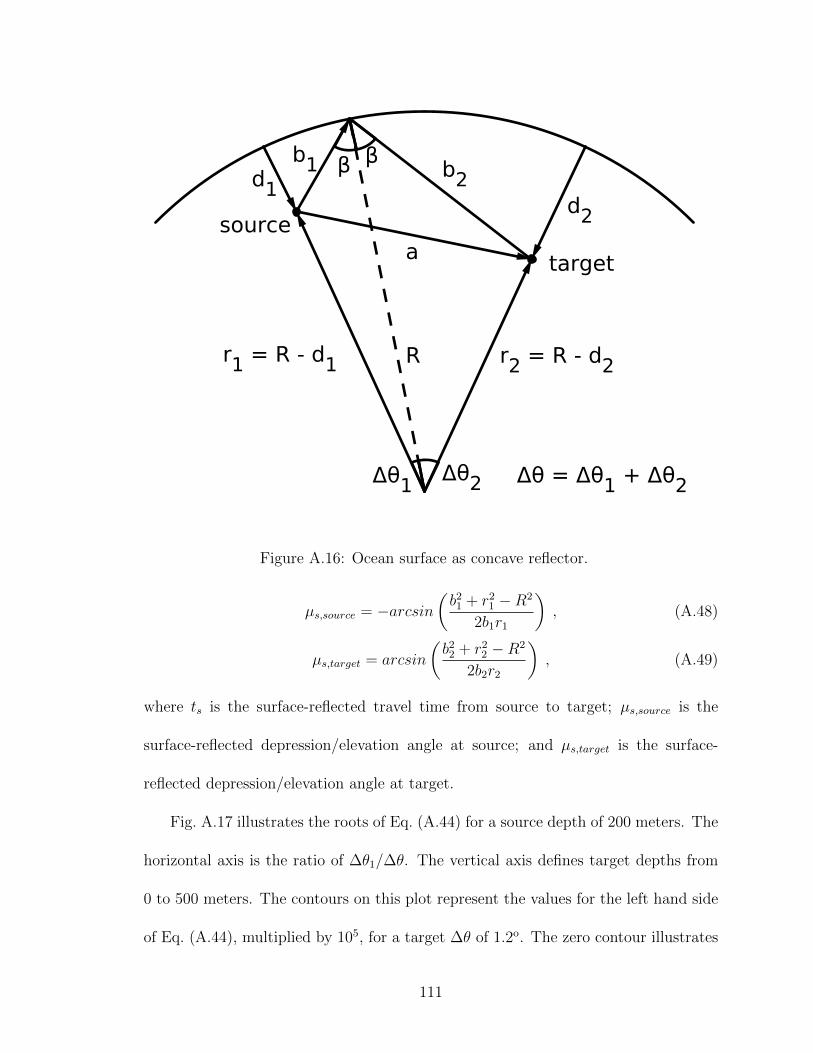
Figure A.16: Ocean surface as concave reflector.

µs,source = −arcsin(b21 + r21 −R2

2b1r1

), (A.48)

µs,target = arcsin

(b22 + r22 −R2

2b2r2

), (A.49)

where ts is the surface-reflected travel time from source to target; µs,source is the

surface-reflected depression/elevation angle at source; and µs,target is the surface-

reflected depression/elevation angle at target.

Fig. A.17 illustrates the roots of Eq. (A.44) for a source depth of 200 meters. The

horizontal axis is the ratio of ∆θ1/∆θ. The vertical axis defines target depths from

0 to 500 meters. The contours on this plot represent the values for the left hand side

of Eq. (A.44), multiplied by 105, for a target ∆θ of 1.2o. The zero contour illustrates

111

−0.0

6−

0.0

6−

0.0

6

−0.0

4−

0.0

4−

0.0

4

−0.04 −0.0

4

−0.0

2−

0.0

2−

0.0

2

−0.02

−0.02

−0.0

2

0

0

0

0

0

0

0.0

2

0.02

0.02

0.0

2

0.04

0.04

0.0

4

0.06

0.0

6

0.0

8

0.0

8

0.1

0.1

20.1

4

Angle to Reflection / Total Angle

Ta

rge

t D

ep

th (

m)

Source=200 m, Target=1.2 deg

0 0.1 0.2 0.3 0.4 0.5 0.6 0.7 0.8 0.9 1−500

−450

−400

−350

−300

−250

−200

−150

−100

−50

0

Figure A.17: Roots of surface reflection transcendental equation.

the location of the roots at each target depth. For example, we found that there are

three roots for ∆θ1 at values of ∆θ times 0.190047203712437, 0.425088688451783, and

0.88486312787168 when a target depth was 150 meters. The physical interpretation

of the multiple roots is that there are multiple surface-reflection paths focused onto

the target location by the concave surface of the earth.

The analytic eigenray products for a target at a depth of 150 m are shown in

Table A.3. WaveQ3D was run with a time step of 100 ms and a depression/elevation

launch angle spacing of 0.05o. The travel times computed by WaveQ3D matched

112

Table A.3: Expected eigenray values for target at 1.2o and 150 m.

Path Travel time Launch angle Target angle

Direct Path 89.05102557 s -0.578554378o +0.621445622o

Surface 1 89.05369537 s +0.337347599o +0.406539112o

Surface 2 89.05379297 s -0.053251329o +0.233038477o

Surface 3 89.05320459 s -0.433973977o -0.48969753o

the analytic result to within 1.2x10-5 s, and the angles were accurate to within

0.012o. Note that rhe launch angle spacing was much tighter than other tests be-

cause WaveQ3D’s eigenray searching logic is limited to finding one ray path between

any two launch angles. A larger launch angle increment in this test would have

caused the model to fail to find the ”Surface 3” path. But with this context, we felt

that WaveQ3D was quite accurate in predicting the travel times and angles for the

equivalent of a Lloyd’s mirror geometry on a spherical earth.

A.5.3 Eigenray robustness for Lloyd’s mirror on spherical

earth

This test extends the results of the previous section by comparing modeled travel

times and ray path angles, for the spherical equivalent of Lloyd’s mirror, at a variety

of depths and ranges. This test used a isovelocity speed of sound of 1500 m/s, a

frequency of 2000 Hz, a source depth of 200 m, target depths from 0 to 1000 m,

181 tangent spaced depression/elevation angles (explained in the Section A.6.2), 1o

spaced azimuth angles from -4o to +4o, and a time step of 100 ms. The maximum

113

range was limited to ∆θ = 0.8o to ensure that only a single surface reflected path

was produced at each target location (see Fig. A.14). This choice allows the test to

be run with a ray spacing that was much more typical than the fine scale D/E angles

used in the previous section.

10−10

10−8

10−6

10−4

10−2

Tra

ve

l T

ime

Err

ors

(s)

10−8

10−6

10−4

10−2

100

So

urc

e D

/E E

rro

rs (

de

g)

0 0.1 0.2 0.3 0.4 0.5 0.6 0.7 0.810

−8

10−6

10−4

10−2

100

Latitude Change (deg)

Ta

rge

t D

/E E

rro

rs (

de

g)

0 m

10 m

100 m

1000 m

Figure A.18: Eigenray errors for Lloyd’s mirror direct path.

The eigenray errors for direct path are summarized in Fig. A.18. Each plot shows

the absolute value of the difference between the WaveQ3D model and the analytic

solution, as a function of range, for targets at depths of 0, 10, 100, and 1000 m.

Beyond a range of 0.1o (about 11 km), the direct path model had maximum errors in

114

travel time error and angle of 0.0087 ms and 0.024o. In each case, these errors were

larger at short ranges. The short range errors were most pronounced near the ocean

surface and at the 1000 m depth.

The eigenray errors for the surface reflected path are shown in Fig. A.19. Once

again, the errors were largest at short ranges, both near the ocean surface and at

the 1000 m depth. Beyond a range of 0.1o, the surface reflected path model has a

maximum travel time error of 0.0041 ms, a maximum source angle error of 0.055o and

a maximum target angle error of 0.047o. In each case, the errors are larger at short

ranges.

The inaccuracies near the surface were attributed to undersampling by the 100 ms

time step, as illustrated in Fig. A.20. The solid lines in this figure represent direct

path rays that are moving out in range and up toward the surface from the source at

200 m. The dashed lines present the same ray paths after reflection from the ocean

surface. The dotted lines that connect them represent discontinuities between the

direct path and surface reflected segments of the wavefront. At short ranges, these

discontinuities cause the edges of ray families to be far from targets that are near

the interface; extrapolation led to inaccuracy. Shortening the time step mitigates

this source of inaccuracy. At longer ranges, this source of inaccuracy is automatically

reduced by the fact that the edges of the ray families get closer to the surface as the

rays become more horizontal.

The errors at large depths were attributed to the tangent spaced depression/elevation

angles used in this test. Using a more uniform scheme for depression/elevation angles

would have mitigated this source of inaccuracy.

115

10−10

10−8

10−6

10−4

10−2

Tra

ve

l T

ime

Err

ors

(s)

10−8

10−6

10−4

10−2

100

So

urc

e D

/E E

rro

rs (

de

g)

0 0.1 0.2 0.3 0.4 0.5 0.6 0.7 0.810

−8

10−6

10−4

10−2

100

Latitude Change (deg)

Ta

rge

t D

/E E

rro

rs (

de

g)

0 m

10 m

100 m

1000 m

Figure A.19: Eigenray errors for Lloyd’s mirror surface reflected path.

A.5.4 Propagation loss accuracy for Lloyd’s Mirror

Near the surface, WaveQ3D must extrapolate eigenrays from distances that are up to

1.5 paths away from the interface. The tests in this section were designed to expose

the impact of this limitations on propagation loss accuracy. The analytic solutions

for these test were derived in Cartesian coordinates using the method of images.

p(r, z) =eikL1

L1

− eikL2

L2

; (A.50)

L1 =√r2 + (z − zs)2 ; (A.51)

116

0 0.01 0.02 0.03 0.04 0.05−50

−45

−40

−35

−30

−25

−20

−15

−10

−5

0

Latitude Change (deg)

Depth

(m

)

5.56 km Range Window

Direct Path

Surface Reflected

Discontinuity

Figure A.20: Time-step effects near the ocean surface.

L2 =√r2 + (z + zs)2 ; (A.52)

where r is the target range; z is the target depth (positive is down); zs is the source

depth (positive is down); L1 is the slant range to source; L2 is the slant range to

image source (above water); k is the acoustic wave number (2πf/c); and f is the

signal frequency; c is the speed of sound; p(r, z) is the complex pressure.

The propagation loss for a 200 meters deep target is shown as a function of range

in Fig. A.21 and Fig. A.22. Results for a 10 km range target are shown as a function

of depth in Fig. A.23. Both cases used a speed of sound of 1500 m/s, with a “flat

117

earth” adjustment from Eq. (A.9), a frequency of 2000 Hz, a source depth of 75 m,

181 tangent spaced depression/elevation angles, 1o spaced azimuth angles from -4o

to +4o, and a time step of 100 ms. Figure A.22 highlights fact that the errors in

Fig. A.21 are most sever at range less than 2 km. Figure A.22 illustrates that fact

that the largest errors, as a function of depth, are right below the ocean surface. We

attribute the ocean surface results to small in the computation of travel time for the

direct and surface reflected paths.

0 1 2 3 4 5 6 7 8 9 10−110

−100

−90

−80

−70

−60

−50

−40

−30

Pro

pagation L

oss (

dB

)

Range (km)

Source Depth=25 m Target Depth=200 m Freq=2000 Hz

PLR

theory

Figure A.21: Lloyd’s mirror propagation loss as a function of range.

To compare these results quantitatively, we will use a set of statistical measures

118

0 0.2 0.4 0.6 0.8 1 1.2 1.4 1.6 1.8 2−110

−100

−90

−80

−70

−60

−50

−40

−30

Pro

pa

ga

tio

n L

oss (

dB

)

Range (km)

Source Depth=25 m Target Depth=200 m Freq=2000 Hz

PLR

theory

Figure A.22: Lloyd’s mirror propagation loss errors at short ranges.

that are defined in detail in Appendix C. The differences between the WaveQ3D

model and the analytic results are summarized in Table A.4. From this, we conclude

that, although the WaveQ3D model’s Lloyd’s Mirror predictions clearly has limita-

tions, those limitations will have a limited impact on its ability to accurately model

propagation loss in a Lloyd’s mirror environment.

119

−110 −105 −100 −95 −90 −85 −80 −75−40

−35

−30

−25

−20

−15

−10

−5

0

Propagation Loss (dB)

De

pth

(m

)

Source Depth=25 m Target Range=10 km Freq=2000 Hz

PLR

theory

Figure A.23: Lloyd’s mirror propagation loss as a function of depth.

A.5.5 Eigneray and propagation loss accuracy in an extreme

downward refraction environment

In this test, the eigneray and propagation loss accuracy of the WaveQ3D model were

analyzed for the extreme n2 linear test case developed by Pedersen and Gordon.32

Two geometries were supported in this test:

• The shallow source geometry puts the source at a depth of 75 m and creates a

series of targets at a depth of 75 m with ranges from 500-1000 m.

120

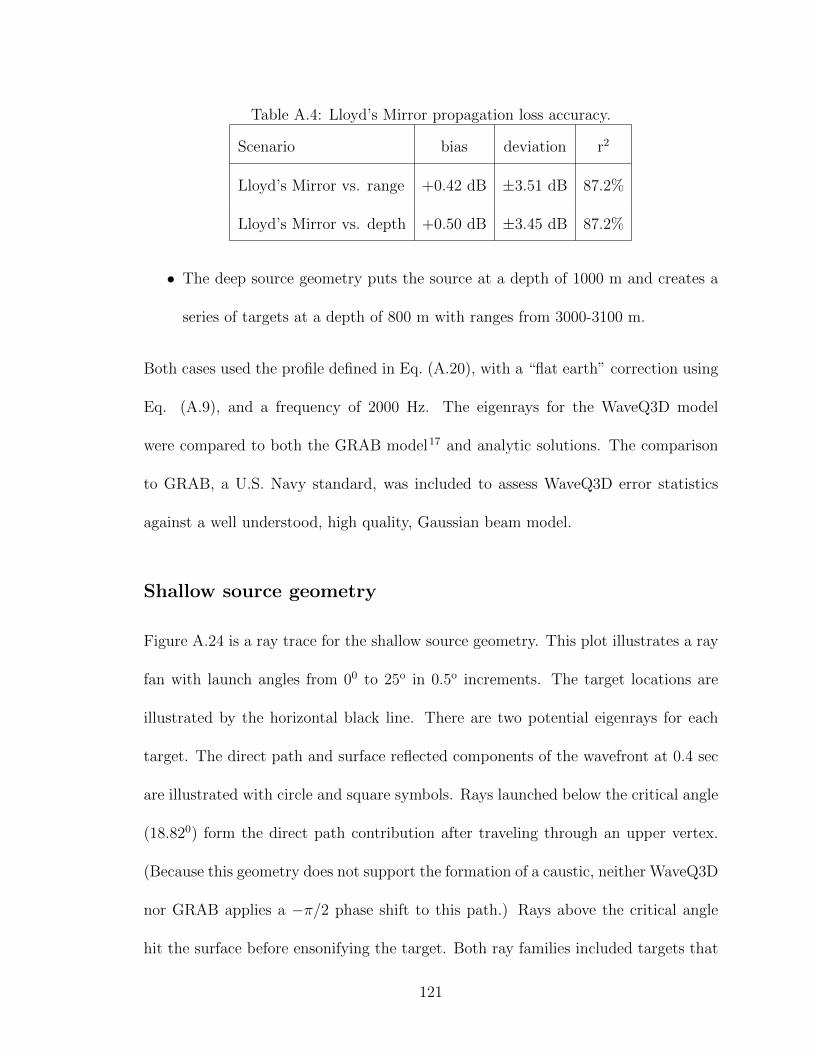
Table A.4: Lloyd’s Mirror propagation loss accuracy.

Scenario bias deviation r2

Lloyd’s Mirror vs. range +0.42 dB ±3.51 dB 87.2%

Lloyd’s Mirror vs. depth +0.50 dB ±3.45 dB 87.2%

• The deep source geometry puts the source at a depth of 1000 m and creates a

series of targets at a depth of 800 m with ranges from 3000-3100 m.

Both cases used the profile defined in Eq. (A.20), with a “flat earth” correction using

Eq. (A.9), and a frequency of 2000 Hz. The eigenrays for the WaveQ3D model

were compared to both the GRAB model17 and analytic solutions. The comparison

to GRAB, a U.S. Navy standard, was included to assess WaveQ3D error statistics

against a well understood, high quality, Gaussian beam model.

Shallow source geometry

Figure A.24 is a ray trace for the shallow source geometry. This plot illustrates a ray

fan with launch angles from 00 to 25o in 0.5o increments. The target locations are

illustrated by the horizontal black line. There are two potential eigenrays for each

target. The direct path and surface reflected components of the wavefront at 0.4 sec

are illustrated with circle and square symbols. Rays launched below the critical angle

(18.820) form the direct path contribution after traveling through an upper vertex.

(Because this geometry does not support the formation of a caustic, neither WaveQ3D

nor GRAB applies a −π/2 phase shift to this path.) Rays above the critical angle

hit the surface before ensonifying the target. Both ray families included targets that

121

were ensonified in their evanescent region, the region outside of the ray fan.

0 0.2 0.4 0.6 0.8 1 1.2−200

−180

−160

−140

−120

−100

−80

−60

−40

−20

0

Range (km)

Dep

th (

m)

direct

surface

Figure A.24: Ray trace for shallow source.

Figures A.25 and A.26 compare the individual WaveQ3D and GRAB eigenrays for

the direct and surface reflected paths. Analytic solutions for the travel time and rays

angles were also computed using Eqn. (A.16) through (A.19). To highlight differences

in travel time, a bulk time has been removed using the slope of the analytic solution

for the direct path.

The GRAB model was configured using ray fan with launch angles from 00 to

25o in 0.1o increments. However, it is important to note that, using the sound speed

122

0.5 0.6 0.7 0.8 0.9 1−90

−80

−70

−60

−50

Range (km)

Pro

pagation L

oss (

dB

)

0.5 0.6 0.7 0.8 0.9 1

0

5

10

Range (km)

Tra

vel T

ime −

Bulk

(sec)

PLR

GRAB

theory

0.5 0.6 0.7 0.8 0.9 18

10

12

14

16

18

20

22

24

Range (km)

Sourc

e D

/E (

deg)

0.5 0.6 0.7 0.8 0.9 1−24

−22

−20

−18

−16

−14

−12

−10

−8

Range (km)

Targ

et D

/E (

deg)

Figure A.25: Direct path eigenrays for shallow source.

at the source, GRAB automatically enhances the fan around the critical with 11

additional beams with spacings of 0o, ±0.03125o, ±0.0625o, ±0.125o, ±0.25o, and

±0.5o. If these small rays spacings were not used near the critical ray, it would lead

to un-realistically large gaps between the outer edge of each ray family and the critical

ray. This is especially true for the surface reflected path in this geometry.

To achieve a similar effect, WaveQ3D was configured with 0.025o spaced depres-

sion/elevation angles from 0o to +25o and 1o spaced azimuth angles from -4o to +4o.

Because this geometry evolves so quickly in time, the WaveQ3D results were created

123

0.5 0.6 0.7 0.8 0.9 1−90

−80

−70

−60

−50

Range (km)

Pro

pagation L

oss (

dB

)

0.5 0.6 0.7 0.8 0.9 1

0

5

10

Range (km)

Tra

vel T

ime −

Bulk

(m

s)

PLR

GRAB

theory

0.5 0.6 0.7 0.8 0.9 18

10

12

14

16

18

20

22

24

Range (km)

Sourc

e D

/E (

deg)

0.5 0.6 0.7 0.8 0.9 1−24

−22

−20

−18

−16

−14

−12

−10

−8

Range (km)

Targ

et D

/E (

deg)

Figure A.26: Surface reflected eigenrays for shallow source.

using a 10 ms time step instead of the 100 ms value used in other tests.

Quantitative results for the shallow source’s individual eigenrays are summarized

in Table A.5. In this table, the maximum difference in travel time, source depres-

sion/elevation angle, and target depression/elevation angle are computed relative to

the analytic solution. Those time and angle comparisons are limited to non-evanescent

regions, where the the analytic solutions had real values. Because our analytic solu-

tion did not support propagation loss for individual eigenrays, WaveQ3D values were

compared to GRAB in this table.

124

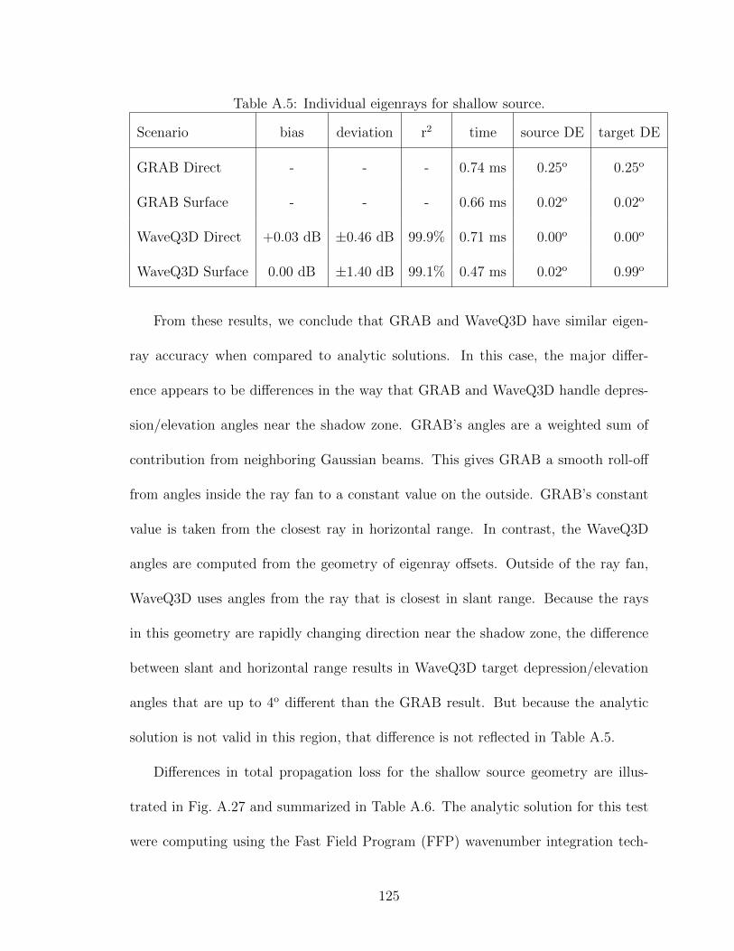
Table A.5: Individual eigenrays for shallow source.

Scenario bias deviation r2 time source DE target DE

GRAB Direct - - - 0.74 ms 0.25o 0.25o

GRAB Surface - - - 0.66 ms 0.02o 0.02o

WaveQ3D Direct +0.03 dB ±0.46 dB 99.9% 0.71 ms 0.00o 0.00o

WaveQ3D Surface 0.00 dB ±1.40 dB 99.1% 0.47 ms 0.02o 0.99o

From these results, we conclude that GRAB and WaveQ3D have similar eigen-

ray accuracy when compared to analytic solutions. In this case, the major differ-

ence appears to be differences in the way that GRAB and WaveQ3D handle depres-

sion/elevation angles near the shadow zone. GRAB’s angles are a weighted sum of

contribution from neighboring Gaussian beams. This gives GRAB a smooth roll-off

from angles inside the ray fan to a constant value on the outside. GRAB’s constant

value is taken from the closest ray in horizontal range. In contrast, the WaveQ3D

angles are computed from the geometry of eigenray offsets. Outside of the ray fan,

WaveQ3D uses angles from the ray that is closest in slant range. Because the rays

in this geometry are rapidly changing direction near the shadow zone, the difference

between slant and horizontal range results in WaveQ3D target depression/elevation

angles that are up to 4o different than the GRAB result. But because the analytic

solution is not valid in this region, that difference is not reflected in Table A.5.

Differences in total propagation loss for the shallow source geometry are illus-

trated in Fig. A.27 and summarized in Table A.6. The analytic solution for this test

were computing using the Fast Field Program (FFP) wavenumber integration tech-

125

0.5 0.55 0.6 0.65 0.7 0.75 0.8 0.85 0.9 0.95 1−80

−75

−70

−65

−60

−55

−50

−45

−40

Range (km)

Pro

pagation L

oss (

dB

)

PLR

GRAB

theory

Figure A.27: Propagation loss for shallow source.

nique.14;6 Note that, in all regions, this implementation of FFP was consistent with an

ideal wave equation solution, except for the presence of some implementation jitter in

the ranges above 880 m. In the region between 500-750 m, all three models produced

almost identical results. As target passed into the shadow zone region, WaveQ3D

and GRAB produced values that were similar to each other, but slightly higher than

FFP. But we also noted that, if a coarser set of depression elevation launch angles was

used for WaveQ3D, the surface reflected path would have disappeared prematurely,

which would have manifested as shadow zone oscillations in the total propagation

126

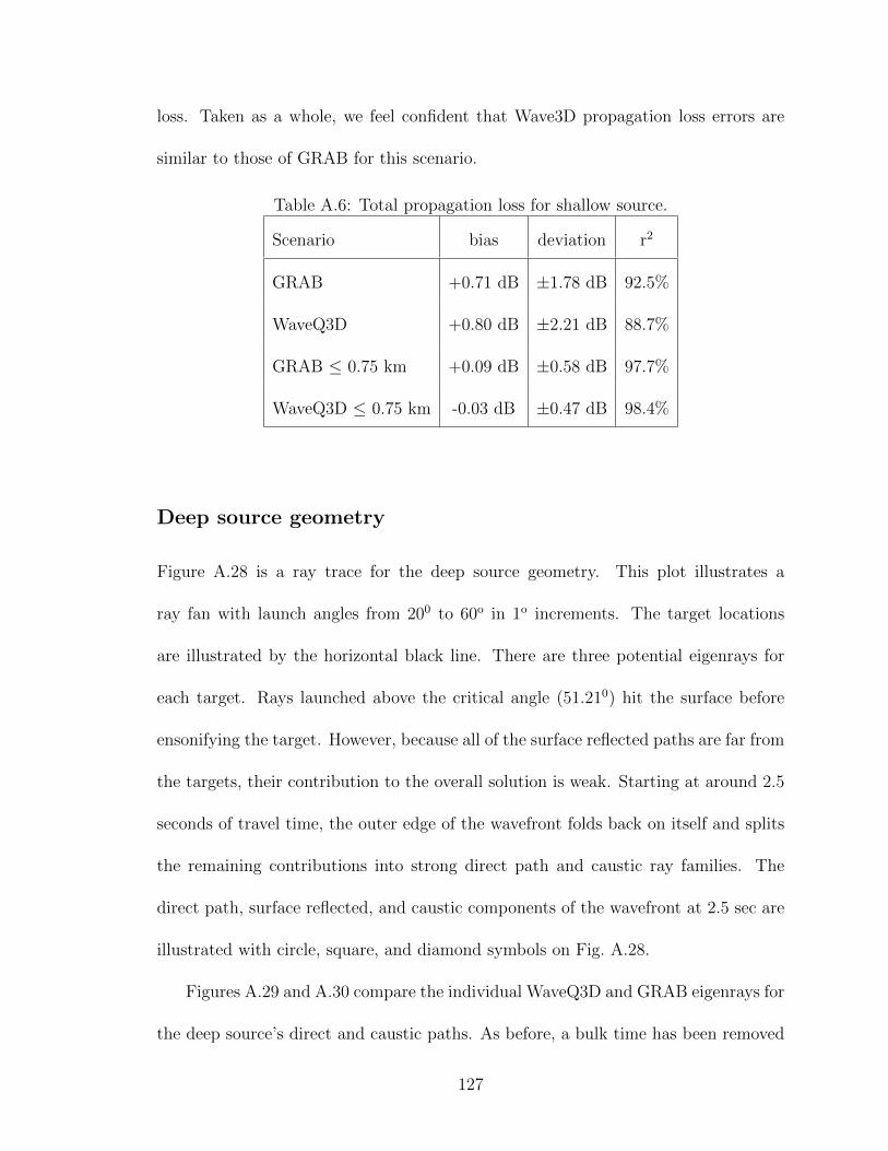
loss. Taken as a whole, we feel confident that Wave3D propagation loss errors are

similar to those of GRAB for this scenario.

Table A.6: Total propagation loss for shallow source.

Scenario bias deviation r2

GRAB +0.71 dB ±1.78 dB 92.5%

WaveQ3D +0.80 dB ±2.21 dB 88.7%

GRAB ≤ 0.75 km +0.09 dB ±0.58 dB 97.7%

WaveQ3D ≤ 0.75 km -0.03 dB ±0.47 dB 98.4%

Deep source geometry

Figure A.28 is a ray trace for the deep source geometry. This plot illustrates a

ray fan with launch angles from 200 to 60o in 1o increments. The target locations

are illustrated by the horizontal black line. There are three potential eigenrays for

each target. Rays launched above the critical angle (51.210) hit the surface before

ensonifying the target. However, because all of the surface reflected paths are far from

the targets, their contribution to the overall solution is weak. Starting at around 2.5

seconds of travel time, the outer edge of the wavefront folds back on itself and splits

the remaining contributions into strong direct path and caustic ray families. The

direct path, surface reflected, and caustic components of the wavefront at 2.5 sec are

illustrated with circle, square, and diamond symbols on Fig. A.28.

Figures A.29 and A.30 compare the individual WaveQ3D and GRAB eigenrays for

the deep source’s direct and caustic paths. As before, a bulk time has been removed

127

0 0.5 1 1.5 2 2.5 3 3.5−1200

−1000

−800

−600

−400

−200

0

Range (km)

De

pth

(m

)

direct

surface

caustic

Figure A.28: Ray trace for shallow source.

using the slope of the analytic solution for the direct path. In these results, the

GRAB model was configured using ray fan with launch angles from 200 to 60o in 0.1o

increments and rays near the caustic were automatically augmented. WaveQ3D used

a ray spacing of 0.25o spacing to achieve a similar result.

The big difference between the models appears to be the fact that the WaveQ3D

transmission loss has a more gradual roll-off into the shadow zones than GRAB.

Quantitative comparisons for the deep source’s individual eigenrays are summarized

in Table A.7. The statistics for the WaveQ3D angles for the caustic path are skewed by

128

3 3.05 3.1−90

−80

−70

−60

−50

Range (km)

Pro

pagation L

oss (

dB

)

3 3.05 3.1

0

5

10

Range (km)

Tra

vel T

ime −

Bulk

(m

s)

PLR

GRAB

theory

3 3.05 3.136

38

40

42

44

46

48

50

52

Range (km)

Sourc

e D

/E (

deg)

3 3.05 3.1−52

−50

−48

−46

−44

−42

−40

−38

−36

Range (km)

Targ

et D

/E (

deg)

Figure A.29: Caustic eigenrays for deep source.

the fact that differences in launch angle resolutions causes inner edge of the WaveQ3D

result to prematurely transition to it shadow zone result. In other regions, the agree-

ment is much closer. It is also important to note that the depression/elevation angle

deviations seen in the WaveQ3D results for the shallow source are less evident in the

deep source case.

Differences in total propagation loss for the deep source geometry are illustrated

in Fig. A.31 and summarized in Table A.8. In the region from 3000 to 3040 meters,

the FFP has stronger oscillations than either the WaveQ3D or GRAB models. This

129

3 3.05 3.1−90

−80

−70

−60

−50

Range (km)

Pro

pagation L

oss (

dB

)

3 3.05 3.1

0

5

10

Range (km)

Tra

vel T

ime −

Bulk

(m

s)

PLR

GRAB

theory

3 3.05 3.136

38

40

42

44

46

48

50

52

Range (km)

Sourc

e D

/E (

deg)

3 3.05 3.1−52

−50

−48

−46

−44

−42

−40

−38

−36

Range (km)

Targ

et D

/E (

deg)

Figure A.30: Direct path eigenrays for deep source.

can be attributed to surface reflected contribution that is stronger in the FFP result

than in either of the Gaussian beam models. At all other ranges, the WaveQ3D and

GRAB results were both a very close fit to FFP’s total propagation loss.

A WaveQ3D anomaly was discovered during the deep source geometry testing.

Errors in the total propagation loss within the shadow zone were frequently seen when

the launch angles finer than 0.01 degrees were used. What we discovered was that at

this spacing, the contribution in the shadow zone was the result of a summation of

over 100 Gaussian beams for both the direct and caustic paths. Small errors in the

130

Table A.7: Individual eigenrays for deep source.

Scenario bias deviation r2 time source DE target DE

GRAB Direct - - - 0.65 ms 0.47o 0.54o

GRAB Caustic - - - 3.77 ms 0.87o 0.98o

WaveQ3D Direct +0.06 dB ±3.17 dB 97.0% 0.64 ms 0.21o 0.24o

WaveQ3D Caustic +1.15 dB ±4.07 dB 94.4% 3.97 ms 1.24o 1.40o

3 3.02 3.04 3.06 3.08 3.1 3.12−80

−75

−70

−65

−60

−55

−50

−45

−40

Range (km)

Pro

pagation L

oss (

dB

)

PLR

GRAB

theory

Figure A.31: Propagation loss for deep source.

calculation of cell width and cell distance to the target appear to accumulate when

the total loss is the result of many weak contributions. For the individual eigenrays,

131

Table A.8: Total propagation loss for deep source.

Scenario bias deviation r2

GRAB -0.95 dB ±3.05 dB 95.4%

WaveQ3D -0.22 dB ±1.94 dB 92.8%

GRAB ≥ 3.04 km -1.45 dB ±3.70 dB 97.0%

WaveQ3D ≥ 3.04 km -0.03 dB ±2.20 dB 94.4%

this anomaly results in a slight broadening of the transmission loss decay tails. But,

since the shape of the outer edge of the total propagation loss depends on destructive

interference between the paths, these errors often resulted in imperfect cancellation,

on the order of -70 dB, in the region between 3090 and 3105 meters. Although these

problems may have been aggravated by the extreme environment, developers should

use extra caution when using WaveQ3D with super-fine ray spacings.

A.6 Derivations

A.6.1 Ray path derivation for concave ocean surface

The analytic solution for the direct-path eigenrays was derived from the laws of sines

and cosines.

a2 = r21 + r22 − 2r1r2cos(∆θ) , (A.53)

td = a/c0 , (A.54)

µd,source = −arcsin(a2 + r21 − r22

2ar1

), (A.55)

132

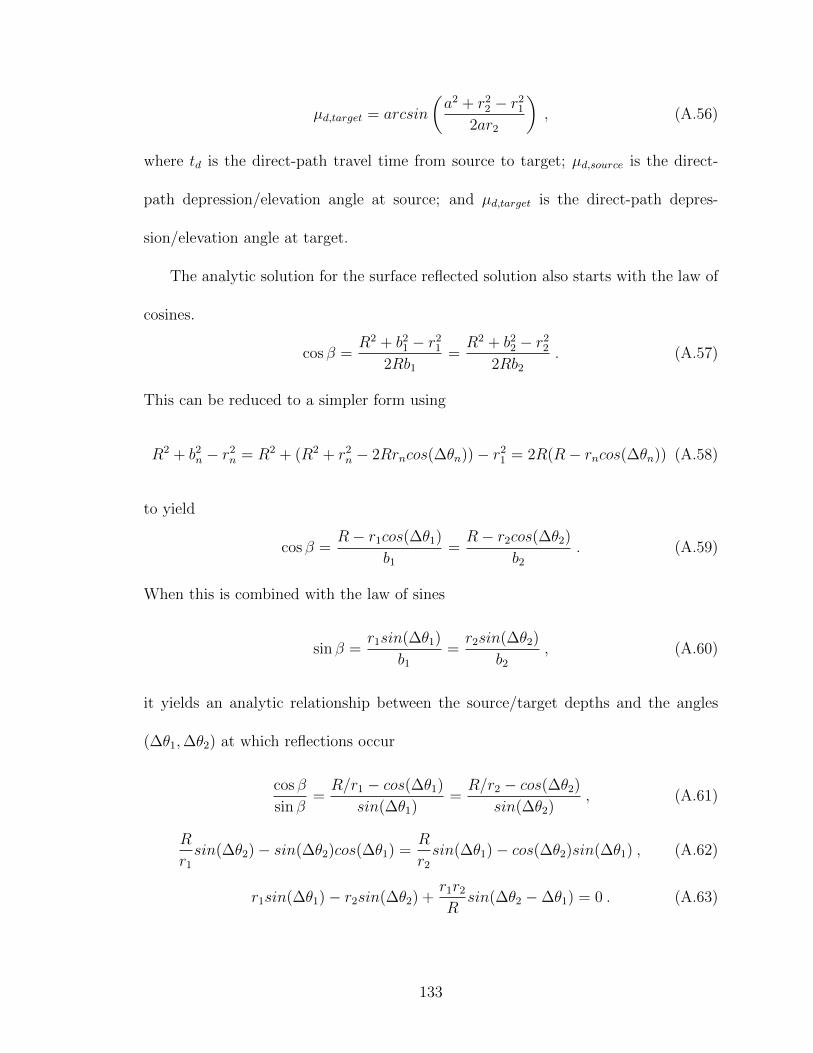
µd,target = arcsin

(a2 + r22 − r21

2ar2

), (A.56)

where td is the direct-path travel time from source to target; µd,source is the direct-

path depression/elevation angle at source; and µd,target is the direct-path depres-

sion/elevation angle at target.

The analytic solution for the surface reflected solution also starts with the law of

cosines.

cos β =R2 + b21 − r21

2Rb1=R2 + b22 − r22

2Rb2. (A.57)

This can be reduced to a simpler form using

R2 + b2n − r2n = R2 + (R2 + r2n − 2Rrncos(∆θn))− r21 = 2R(R− rncos(∆θn)) (A.58)

to yield

cos β =R− r1cos(∆θ1)

b1=R− r2cos(∆θ2)

b2. (A.59)

When this is combined with the law of sines

sin β =r1sin(∆θ1)

b1=r2sin(∆θ2)

b2, (A.60)

it yields an analytic relationship between the source/target depths and the angles

(∆θ1,∆θ2) at which reflections occur

cos β

sin β=R/r1 − cos(∆θ1)

sin(∆θ1)=R/r2 − cos(∆θ2)

sin(∆θ2), (A.61)

R

r1sin(∆θ2)− sin(∆θ2)cos(∆θ1) =

R

r2sin(∆θ1)− cos(∆θ2)sin(∆θ1) , (A.62)

r1sin(∆θ1)− r2sin(∆θ2) +r1r2R

sin(∆θ2 −∆θ1) = 0 . (A.63)

133

The analytic solutions for the surface reflected path requires finding values of ∆θ1

which solve the transcendental equation

r1sin(∆θ1)− r2sin(∆θ −∆θ1) +r1r2R

sin(∆θ − 2∆θ1) = 0 . (A.64)

A.6.2 Tangent spaced depression/elevation angles

0 1 2 3 4 5 6 7 8 9 10−200

−150

−100

−50

0

Depth

(m

)

45 uniformly spaced rays

0 1 2 3 4 5 6 7 8 9 10−200

−150

−100

−50

0

Range (km)

Depth

(m

)

45 tangent spaced rays

Figure A.32: Tangent spaced beams.

Because sonar detection ranges are often much longer than the depths of interest,

there is frequently a need to emphasis propagation paths near the horizontal. The

GRAB model17 manages this requirement by automatically adding rays in the de-

134

pression/elevation directions needed to support caustics, surface ducts, and SOFAR

channels. The WaveQ3D model currently does not support any such automatic ray

adjustment; but it does support any ray spacing that is monotonically increasing.

Tangent spaced depression/elevation angles will be used frequently in the eigenray

and propagation loss testing for WaveQ3D. As shown in the top panel of Fig. A.32,

uniformly spaced rays in an isovelocity environment severely under-sample the direct

path contributions at ranges beyond a few kilometers. When the ray paths are ini-

tialized such that the tangents of the launch angles are uniformly spaced (bottom

panel), the long range contributions are better supported. Of course, this improve-

ment comes at the expense of short range contributions. But, that trade-off often

matches the requirements of sonar simulations.

To generate a set of N tangent spaced beams µ[n], over the interval [µ1, µN ], with

the densest spacing at µc, WaveQ3D uses the following algorithm

a1 = arctan

(µ1 − µc

σ

)(A.65)

aN = arctan

(µN − µc

σ

)(A.66)

x[n] = a1 +aN − a1N − 1

n for n = 0, 1, 2, ..., N-1 (A.67)

µ[n] = µc + σ tan(x[n]) (A.68)

where σ is an arbitrary scaling factor. WaveQ3D testing frequently uses 181 tangent

spaced depression/elevation rays, from -90o to +90o, with µc = 0o and σ = 6. This

combination of factors yields a ray fan with maximum resolution of about 0.1o and

85% of its rays in the ±20o range.

135

A.6.3 Propagation loss error statistics

We would like to define quantitative differences between modeled and analytic prop-

agation losses in a way that illuminates the suitability of the model for real-time,

sonar simulation/stimulation systems. To that end, we define the following statistical

measures

b[PL] =1

N

N∑n=1

(PLmodel[n]− PLtheory[n]) , (A.69)

ψ2[PL] =1

N

N∑n=1

(PLmodel[n]− PLtheory[n])2 , (A.70)

s[PL] =√ψ2[PL]− b2[PL] , (A.71)

x[n] = PLtheory[n]− 1

N

N∑n′=1

(PLtheory[n′] , (A.72)

y[n] = PLmodel[n]− 1

N

N∑n′=1

(PLmodel[n′] , (A.73)

r2[PL] =

(N∑n=1

x[n]y[n]

)2

N∑n=1

x2[n]N∑n=1

y2[n]

× 100% , (A.74)

where PLmodel[n] and PLtheory[n] are the samples in the model and theory in dB

units; b[PL] is the estimated bias between the model and the theory; s[PL] is the

estimated deviation between the model and the theory; and r2[PL] is the coefficient

of determination between the model and the theory.

The active sonar equation can be expressed in the form

SE = FOM − 2PL , (A.75)

FOM = SL+ TS −NL+DI −DT , (A.76)

136

where SE is the signal excess; PL is the propagation loss; FOM is the active figure

of merit; SL is the source level; TS is the target strength; NL is the noise level; DI is

the directivity index; and DT is the detection threshold.42 If we assume that errors

in the figure of merit are handled separately, then 2b[PL] and s2[PL] are estimates of

signal excess bias and variance. The coefficient of determination, r2[PL], estimates

how well the modeled signal excess’ shape is correlated to an ideal solution.

A.7 Summary

This paper represents an important milestone the development of the WaveQ3D

model. A suite of tests were developed to quantitatively compare the ray tracing,

reflection, eigenray finding, and propagation loss elements of the model to analytic

solutions. Hopefully, this approach will help other researchers evaluate the capabil-

ity and limitations of the WaveQ3D model and provide a firm foundation to move

forward with further testing.

This testing also led to the development of a few general guidelines for the use of

the WaveQ3D model.

• Using a time step size as coarse as 100 ms seems to produce accurate results

for most applications. However, this step size should be decreased to 10 ms

for applications that need high accuracy at ranges less than 2 km. This is

particularly true for applications that are interested in effects near the ocean

surface, or directly below the source.

• The selection of launch angles can have a significant effect on propagation loss

137

results. Like all models that as based on ray theory, WaveQ3D can miss fea-

tures in the environment because of spatial under-sampling. Tangent spaced

depression/elevation angles appear to improve WaveQ3D model performance

for scenarios dominated by horizontal paths. Uniform spacing is suggested for

applications that need high accuracy at ranges less than 2 km.

• The WaveQ3D model is designed to be computationally efficient when comput-

ing transmission loss for up to 100 targets, at multiple frequencies, in a fully

3-D environment. But because the WaveQ3D eigenray detection process is less

efficient than an equivalent calculation in Cartesian coordinates, WaveQ3D can

actually be much slower than other models when thousands of range/depth

combinations are required. Applying the WaveQ3D model in 2-D environments

is also not very efficient.

A.8 Acknowledgments

This paper was developed as part of Sean Reilly’s PhD studies at the Ocean Engi-

neering Department of the University of Rhode Island, under the direction of Dr.

Gopu Potty and Dr. James Miller. This verification testing effort was funded by the

High Fidelity Active Sonar Training (HiFAST) Project at the U.S. Office of Naval

Research.

138

Bibliography

[1] A. Alvera-Azcarate, A. Barth, M. Rixen, J.M. Beckers, ”Reconstruction of in-

complete oceanographic data sets using empirical orthogonal functions: applica-

tion to the Adriatic Sea surface temperature”, Ocean Modelling (2005), vol. 9,

iss. 4, pp. 325-346.

[2] A. Alvera-Azcarate, A. Barth, D. Sirjacobs, F. Lenartz And J.M. Beckers, ”Data

Interpolating Empirical Orthogonal Functions (DINEOF): a tool for geophysi-

cal data analyses”, International Conference on Marine Data and Information

Systems - IMDIS, Athens, 2008

[3] M. S. Ballard, Y. Lin, J. F. Lynch, Horizontal refraction of propagating sound

due to seafloor scours over a range-dependent layered bottom on the New Jersey

shelf, J. Acoust. Soc. Amer. 131 (2012) pp. 2587-2598.

[4] M. S.Ballard, Modeling three-dimensional propagation in a continental shelf en-

vironment. J. Acoust. Soc. Amer. 131 (2012) pp. 1969-1977.

[5] P. A. Baxley, H. Bucker, M. B. Porter, Comparison of Beam Tracing Algorithms,

Proceedings of the Fifth European Conference on Underwater Acoustics (ECUA)

2000.

139

[6] L. M. Brekhovskikh, Waves in Layered Media (Academic Press Inc., New York,

1980), 2nd Edition, Section 54.

[7] M. J. Buckingham, Theory of acoustic propagation around a conical seamount,

J. Acoust. Soc. Amer. 80 (1986) pp. 265-277.

[8] T. Burns, S. Reilly, D. Thibaudeau, WaveQ3D-AP Module Root Cause Accuracy

Analysis, report prepared for NAWCTSD, April 2014

[9] V. Cerveny, M. M. Popov, and I. Psencık, Computation of wave fields in inho-

mogeneous media - Gaussian beam approach, Geophys. J. R. Astron. Soc. 70

(1982) 109.

[10] V. Cerveny, Seismic Ray Theory, (Cambridge University Press, New York,

2001), pp.174-178.

[11] M. B. Chrissis, M. Konrad, S. Shurm, CMMI Guidelines for Process Inte-

gration and Product Development, Second Edition, (Addison-Wesley, New

York, 2007).

[12] NOAA National Geophysical Data Center (NGDC), ”U.S. Coastal Relief

Model,” [Online]. Available: http://www.ngdc.noaa.gov/mgg/coastal/crm.html

[Accessed 02/25/2016].

[13] G. B. Deane and M. Buckingham, An analysis of the three-dimensional sound

field in a penetrable wedge with a stratified fluid or elastic basement,J. Acoust.

Soc. Amer. 93 (1993). J. Acoust. Soc. Am., vol. 93, no. 3, pp. 1319-1328, March

1993.

140

[14] F. R. DiNapoli, R. L. Deavenport, Theoretical and numerical Green’s function

field solution in a plane multilayered medium, J. Acoust. Soc. Amer. 67 (1980).

[15] ETOPO1v2 Global Gridded 2-minute Database, National Geophysical Data Cen-

ter, National Oceanic and Atmospheric Administration, U.S. Dept. of Com-

merce [Online]. Available: http://www.ngdc.noaa.gov/mgg/global/global.html

[Accessed 4/14/2016].

[16] FAI Sporting Code, Federation Aeronautique Internationale (FAI), Lausanne,

Switzerland, 16 October 2014.

[17] Software Requirements Specification/Software Design Description and Software

Test Description for the Oceanographic and Atmospheric Master Library Navy

Standard Comprehensive Acoustic System Simulation Model Version 4.2A, Naval

Meteorology and Oceanography Command Report OAML-SRS-SDD-STD-83D

(2008).

[18] K. D. Heaney, J. J. Murray, Measurements of three-dimensional propagation in a

continental shelf environment, J. Acoust. Soc. Amer. 125 (2009) pp. 1394-1402.

[19] K. D. Heaney, J. J. Murray, Measurements of three-dimensional propagation in a

continental shelf environment, J. Acoust. Soc. Amer. 125 (2009) pp. 1394-1402.

[20] K. D. Heaney, R. L. Campbell and J. J. Murray, ”Comparison of hybrid three-

dimensional modeling with measurements on the continental shelf,” J. Acoust.

Soc. Amer., vol. 2, no. 131, pp. 1680-1688, February 2012.

141

[21] F. B. Jensen, W. A. Kuperman, M. B. Porter, and H. Schmidt, Computational

Ocean Acoustics, American Institute of Physics Press, New York, 1994, pp.

150-153.

[22] Y. Jiang, N. R. Chapman and H. A. DeFerrari, Geoacoustic inversion of broad-

band data by matched beam processing, J. Acoust. Soc. Amer. vol. 6, no. 119,

pp. 3707-3706, June 2006.

[23] R. M. Jones, J.P. Riley, T.M. Georges, HARPO: A Versatile Three-Dimensional

Hamiltonian Ray-Tracing Program for Acoustics Waves in an Ocean with Irregu-

lar Bottom, National Oceanic and Atmospheric Administration (NOAA) Report,

(1986).

[24] D. Lee, M. H. Schultz, Numerical Ocean Acoustic Propagation in Three

Dimensions, World Scientific, New York, 1995.

[25] Y. T. Lin, T. F. Duda, A, E. Newhal, Three-Dimensional Sound Propagation

Models Using the Parabolic-Equation Approximation and the Split-Step Fourier

Method, J. Comput. Acoust. 21 (2013)

[26] A. Ben-Menahem and J. S. Sarva, Seismic Waves and Sources, Springer-

Verlag, New York, 1981, pp. 495-502.

[27] CAPT J. Morgan, J. Anti-Submarine Warfare, A Phoenix for the Future. Under-

sea Warfare, The Official Magazine of the Submarine Force, 1988 [Online]. Avail-

able: http://www.public.navy.mil/subfor/underseawarfaremagazine/Issues/

Archives/issue 01/anti.htm [Accessed 4/14/2016].

142

[28] W. H. Munk, Sound channel in an exponentially stratified ocean, with application

to SOFAR, J. Acoust. Soc. Amer. 55 (1974) pp. 220-226.

[29] Naval Air Warfare Center Training Systems Division. Solicitation N61340-13-

R-1057: Live, Virtual, Constructive Modeling and Simulation (LVCMS)/Anti-

Submarine Warfare Virtual At-Sea Training Systems (ASW VAST), Sept 2013.

[30] H. B. Nguyen, H. A. DeFerrari, N. J. Williams and W. A. Venezia, ”Ocean

Acoustic Sensor Installation at the South Florida Ocean Measurement Center,”

IEEE J. Ocean. Eng., vol. 27, no. 2, pp. 235-244, April 2002.

[31] Ocean Acosutics Library, U.S. Office of Naval Research, Ocean Acoustics Pro-

gram [Online]. Available: http://oalib.hlsresearch.com [Accessed 4/14/2016].

[32] M. A. Pedersen, D. F. Gordon, Normal-Mode and Ray Theory Applied to Un-

derwater Acoustic conditions of Extreme Downward Refraction, J. Acoust. Soc.

Amer. 51 (1972) 323.

[33] C. L. Pekeris, Accuracy of the Earth-Flattening Approximation in the Theory

of Microwave Propagation, Phys. Rev. 70 (1943).

[34] M. B. Porter, H. P. Bucker, Gaussian beam tracing for computing ocean acoustic

fields, J. Acoust. Soc. Amer. 93 (1987) 1349.

[35] M. B. Porter, Y. C. Liu, Finite Element Ray Tracing, International Conference

on Theoretical and Computational Acoustics (ICTCA) Volume 2 (1994) 947.

[36] M.B.Porter, The KRAKEN Normal Mode Program (DRAFT), A

143

Deep Water Problem: the Munk Profile (1997) [Online]. Available:

http://oalib.hlsresearch.com/Modes/AcousticsToolbox/manual html/node8.html

[Accessed 4/14/2016].

[37] W. Press, S. Teukolsky, W. Vetterling, B. Flannery, Numerical Recipes in C

(Cambridge University Press, New York, 1992), pp 747-752.

[38] S. M. Reilly, G. R. Potty, M. Goodrich, Computing Acoustic Transmission Loss

Using Three-Dimensional Gaussian Ray Bundles in Geodetic Coordinates, J.

Comp. Acous. 24, March 2016.

[39] L.F. Shampine, Vectorized Adaptive Quadrature in MATLAB, J. Comput. Appl.

Math. 70 (2008).

[40] J. L. Spiesberger, Ocean acoustic tomography: travel time biases, J. Acoust. Soc.

Amer. 77 (61), 1984, pp. 83-100.

[41] F. Sturm, S. Ivansson, Y. M. Jiang, N. R. Chapman, Numerical investigation of

out-of-plane sound propagation in a shallow water experiment, J. Acoust. Soc.

Amer. 124 (2008) pp. 341-346.

[42] R. J. Urick, Principles of underwater sound, 3rd edittion, McGraw-Hill,

New York (1983).

[43] Under Sea Modeling Library development project,

GitHub repository hosting service [Online]. Available:

https://github.com/campreilly/UnderSeaModelingLibrary [Accessed

4/14/2016].

144

[44] T. Veldhuizen, ”Expression Templates,” C++ Report, Vol. 7 No. 5 June 1995,

pp. 26-31

[45] H. Weinberg, R. E. Keenan, Gaussian ray bundles for modeling high-frequency

propagation loss under shallow-water conditions, J. Acoust. Soc. Amer. 100

(1996) 1421.

[46] WGS 84 Implementation Manual, Version 2.4, European Organization for the

Safety of Air Navigation, and the Institute of Geodesy and Navigation, (1998).

[47] E. Williams, Aviation Formulary V1.46 [Online]. Available:

http://williams.best.vwh.net/avform.htm [Accessed 4/14/2016].

[48] World Ocean Atlas 2009, National Oceanographic Data Center, National

Oceanic and Atmospheric Administration, U.S. Dept. of Commerce [Online].

Available: https://www.nodc.noaa.gov/OC5/WOA09/pr woa09.html [Accessed

4/14/2016].

[49] Yakowitz and Szidarovszky, An Introduction to Numerical Computation

(Macmillan Publishing, New York, 1986) pp. 306-311.

145