
Wavelet theory demystified - Signal Processing, IEEE Transactions on
Upload
duongkhanhCategory
view
218download
0
734 IEEE TRANSACTIONS ON INFORMATION THEORY, VOL. 48, NO. 3, MARCH 2002
Wavelet DeconvolutionJianqing Fan and Ja-Yong Koo
Abstract—This paper studies the issue of optimal deconvo-lution density estimation using wavelets. The approach takenhere can be considered as orthogonal series estimation in themore general context of the density estimation. We explore theasymptotic properties of estimators based on thresholding ofestimated wavelet coefficients. Minimax rates of convergenceunder the integrated square loss are studied over Besov classes
of functions for both ordinary smooth and supersmoothconvolution kernels. The minimax rates of convergence depend onthe smoothness of functions to be deconvolved and the decay rateof the characteristic function of convolution kernels. It is shownthat no linear deconvolution estimators can achieve the optimalrates of convergence in the Besov spaces with 2 when theconvolution kernel is ordinary smooth and super smooth. If theconvolution kernel is ordinary smooth, then linear estimatorscan be improved by using thresholding wavelet deconvolutionestimators which are asymptotically minimax within logarithmicterms. Adaptive minimax properties of thresholding waveletdeconvolution estimators are also discussed.
Index Terms—Adaptive estimation, Besov spaces, Kullback–Leibler information, linear estimators, minimax estimation,thresholding, wavelet bases.
I. INTRODUCTION
DECONVOLUTION is an interesting problem which arisesoften in engineering and statistical applications. It pro-
vides a simple structure for understanding the difficulty of ill-conditioned problems and for studying fundamental propertiesof general inverse problems. The deconvolution problem can beformulated as follows. Suppose we haveindependent obser-vations having the same distribution as that ofavailable to estimate the unknown densityof a random vari-able , where
and has a known distribution. Assume furthermore that therandom variables and are independent. Then, the proba-
Manuscript received August 1, 1999; revised March 8, 2001. The work ofJ. Fan was supported in part by the National Science Foundation (NSF) underGrant DMS-0196041 and by RGC under Grant CUHK 4299/00P of HKSAR.The work of J.-Y. Koo was supported by KOSEF under Grant 980701-0201-3.The material in this paper was presented in part at the Autumn Conference of theKorean Statistical Society, National Statistical Office, Korea, November 6–7,1998.
J. Fan is with the Department of Statistics, Chinese University of Hong Kong,Shatin, Hong Kong (e-mail: [email protected]).
J.-Y. Koo is with the Department of Statistics, Hallym University, Chunchon,Kangwon-Do 200-702, Korea (e-mail: [email protected]).
Communicated by J. A. O’Sullivan, Associate Editor for Detection and Esti-mation.
Publisher Item Identifier S 0018-9448(02)01057-X.
bility densities and of and , respectively, are related bya convolution equation
where is the density function of the contaminating error.The function is called the convolution kernel. Our deconvo-lution problem is to estimate the unknown density functionbased on observations from the density.
Models of measurements contaminated with error exist inmany different fields and have been widely studied in both theo-retical and applied settings. Nonparametric deconvolution den-sity estimation is studied in [3], [6], [10]–[12], [16]–[19], [21],[23], [28], and [32], among others. In particular, the optimalrates of convergence are derived in [3], [11], [12], [18], and [32].Masry [22] extends the study to stationary random processesand Hengartner [14] studies Poisson demixing problems. Re-cently, a number of authors have employed wavelet techniquesfor nonparametric inverse problems [1], [7], [15], [25], [29]. Inparticular, Pensky and Vidakovic [25] study linear wavelet de-convolution density estimators for the Sobolev classes of densityfunctions. Nonparametric deconvolution problems have impor-tant applications in statistical errors-in-variables regression [4],[13].
This paper focuses on nonparametric deconvolution densityestimation based on wavelet techniques. This allows us to takefull advantages of sparse representations of functions in Besovspaces by wavelet approximations. As a result, deconvolutionwavelet estimators have better ability in estimating local fea-tures such as discontinuities and short aberrations. They can es-timate functions in the Besov spaces better than the conventionaldeconvolution kernel estimators.
Let be an orthogonal scaling function andbe its corre-sponding wavelet function [5], [24]. Set
and
For each , the family
forms an orthogonal basis for . For the unknown density, it can be decomposed as
For ordinary smooth convolution kernels with degree of smooth-ness , it will be shown that behave like thevaguelettes which are described for several homogeneous oper-ators in [7]. Examples of homogeneous operators include inte-gration and Radon operators. The vaguelettes for homogeneous
0018–9448/02$17.00 © 2002 IEEE

FAN AND KOO: WAVELET DECONVOLUTION 735
operators can be expressed by dilations and translations of afixed function [7]. Since the convolution operator mappingto is inhomogeneous, the family of functionscannot in general be expressed by dilations and translations of afixed function. However, for each fixed, they are translation ofa fixed function, which is enough to derive asymptotic results forwavelet deconvolution. A similar result holds for supersmoothconvolution kernels.
Our approach to the deconvolution density estimation is asfollows. Observe that
(1)
where is the Fourier transform of and andare the characteristic functions of the random variablesand, respectively. The unknown characteristic function can be
estimated from the observed data via the empirical character-istic function. This can be used to provide an unbiased estimateof . Using only the estimated to construct estima-tors of yields so-called linear estimators. The linear decon-volution estimators behave quite analogously to deconvolutionkernel density estimators. They cannot be optimal for functionsin general Besov spaces, no matter how high the resolution level
is chosen. This drawback can be ameliorated by using non-linear thresholding wavelet estimators. Estimate the coefficients
in an analogous manner to keep estimated coeffi-cients only when they exceed a given thresholding level and usethe wavelet decomposition to construct an estimate of density
. The resulting thresholding wavelet estimators are capable ofestimating functions in the Besov spaces optimally, within a log-arithmic order, in terms of the rates of convergence.
The difficulty of deconvolution depends on the smoothnessof the convolution kernel and the smoothness of the func-tion to be deconvolved. This was first systematically studiedin [11] for functions in Lipschitz classes. We will show that theresults continue to hold for the more general Besov classes offunctions. The smoothness of convolution kernels can be char-acterized as ordinary smooth and supersmooth [11]. When aconvolution kernel is ordinary smooth, we will establish theoptimal rates of convergence for both linear estimators and allestimators. They are of polynomial order of sample size. Fur-thermore, we will show that no linear estimators can achievethe optimal rate of convergence for certain Besov classes offunctions, whereas the thresholding wavelet deconvolution es-timators can. This clearly demonstrates the advantages of usingwavelets thresholding procedure and is an extension of the phe-nomenon proved by [8] for nonparametric density estimation.When the error distribution is supersmooth, we will show thatthe optimal rates of convergence are only of logarithmic order ofthe sample size. In this case, while the linear wavelet estimatorscannot be optimal, thresholding wavelet estimators do not pro-vide much gain for estimating functions in the Besov spaces.The reason is that the last resolution level in the thresholdingwavelet estimators has to be high enough in order to reduce ap-proximation errors, but this creates very large variance in the
estimated wavelet coefficients when convolution kernels are su-persmooth.
Since the wavelet deconvolution estimators proposed here areof a form of orthogonal series estimator, there is no guaranteethat such estimators are in the space of densities. It would beworthwhile to investigate deconvolution methods guaranteeingthat the estimators are in the space of densities [17].
The rest of this paper is organized as follows. In Section II, weintroduce some necessary properties on wavelets, Besov norm,and smoothness of convolution kernels. Technical conditionsare also collected in Section II. Minimax properties of linearwavelet estimators are studied in Section III. Section IV de-scribes minimax rates of thresholding wavelet estimators. Adap-tive results are studied in Section V.
II. PRELIMINARY
A. Notation
Let , , and denote expectation, probability, and vari-ance of random variables, respectively. Let denote the thderivative of a function and denote by the space of func-tions having all continuous derivatives with . Weuse the notation
for a given function , where . Let be a generic con-stant, which may differ from line to line. For positive sequences
and , let mean that .Denote by the Fourier transform of a function, defined by
The -distance from density to density is defined by
For any two probability measures and , their Kullback–Leibler information is defined by
if is absolutely continuous with respect to; otherwise,.
B. Wavelets
Recall that one can construct a functionsatisfying the fol-lowing properties [5], [24]. The sequence
is an orthonormal family of ; the function
and

736 IEEE TRANSACTIONS ON INFORMATION THEORY, VOL. 48, NO. 3, MARCH 2002
where denotes the closed subspace spanned by
The function with these properties is called an orthogonalscaling function having regularityfor the multiresolution anal-ysis .
By the construction of the multiresolution analysis
Define the space by
Under the above conditions, there exists a function(the“mother wavelet”) having the following properties:
is an orthonormal basis of and
is an orthonormal basis of ; . Furthermore, ifhas a compact support, so does the wavelet function. Finally,if , then has vanishing moments
for
see [5, Corollary 5.5.2].From the above construction, the sequence
is an orthogonal basis for for each , and for each given
forms an orthogonal basis for . For the probability density, it admits a formal expansion
The coefficients and are called the wavelet coeffi-cients of .
C. Besov Spaces
Let be the associated orthogonal projection operator ontoand . Besov spaces depend on three param-
eters: , , and and are denoted by. Say that if and only if the norm
(with usual modification for ). Using the decompositions
the Besov space can be defined via the equivalent norm
where
Here we have set
and the same notation applies to the sequence . Abusingthe notation slightly, we will also write for the abovesequence norm applied to the wavelet coefficients.
The Besov spaces have the following simple relationship:
for or and
and
for and
They include the Sobolev spaces and bounded-Lipschitzfunctions for .
Set
The spaces of densities we consider are defined by
and
where and are given constants.
D. Error Distributions
The asymptotic properties of proposed deconvolution waveletestimators can be characterized by two types of error distribu-tions according to [11]: ordinary smooth and supersmooth dis-tributions. Let
be the characteristic function of a random variable. We callthe distribution of the random variablethe ordinary smooth oforder if satisfies
as
for some positive constants , and nonnegative . Ex-amples of ordinary smooth distributions include Gamma,symmetric Gamma distributions (including double exponentialdistributions). We call the distribution of a random variablesupersmooth of order if satisfies
as for some positive constants , , , , andconstants and . The supersmooth distributions includeGaussian, mixture Gaussian, and Cauchy distributions.
E. Technical Conditions
To facilitate our presentation, we collect all technical condi-tions that will be needed in this section. These conditions are
FAN AND KOO: WAVELET DECONVOLUTION 737
not necessarily independent and can even be mutually exclusive.Indeed, some of them are stronger than others. We first collectconditions needed for scaling functions and wavelet functions.
(A1) The functions and are compactly supported.
(A2) The functions , where and .
(A3) .
(A4) The supports of and are and, respectively.
(A5) For every integer and , there exists apositive constant such that
and
References [5] and [24] contain examples of scaling functionssatisfying the above conditions. In particular, Daubechies’wavelets satisfy (A1)–(A3) and Meyer’s wavelets (A4) and(A5). When the error distributions are ordinary smooth,Daubechies’ wavelets will be used. On the other hand, Meyer’swavelets are adopted for the supersmooth error distributions.
We need the following conditions for the convolution kernelsthat are ordinary smooth. Double exponential and Gamma dis-tributions satisfy the following conditions. It can be noted thatcondition (B2) implies that for any .
(B1) .
(B2) .
(B3) , for .
When the error distribution is supersmooth, the followingconditions are required.
(C1) for some positiveconstants and and some constant .
(C2) as forsome , .
(C3) for some positiveconstants and and a constant .
(C4) For
with and a constant.
If is Normal or Cauchy, then (C1)–(C3) are satisfied. TheNormal error distribution satisfies condition (C4) with .We note that condition (C3) implies that for any .
III. L INEAR WAVELET DECONVOLUTION ESTIMATOR
In this section, we plan to establish the minimax rate for thebest linear estimator under the integrated square loss. This isachieved by first establishing a minimax lower bound over theclass of linear deconvolution estimators and by proposing lineardeconvolution wavelet estimators that achieve this lower bound.From the results in this and the next section, we will see that thelinear estimators can be optimal only when the function class isSobolev, a special case of the Besov space . For the general
Besov space with , no linear estimators can achievethe optimal rates of convergence.
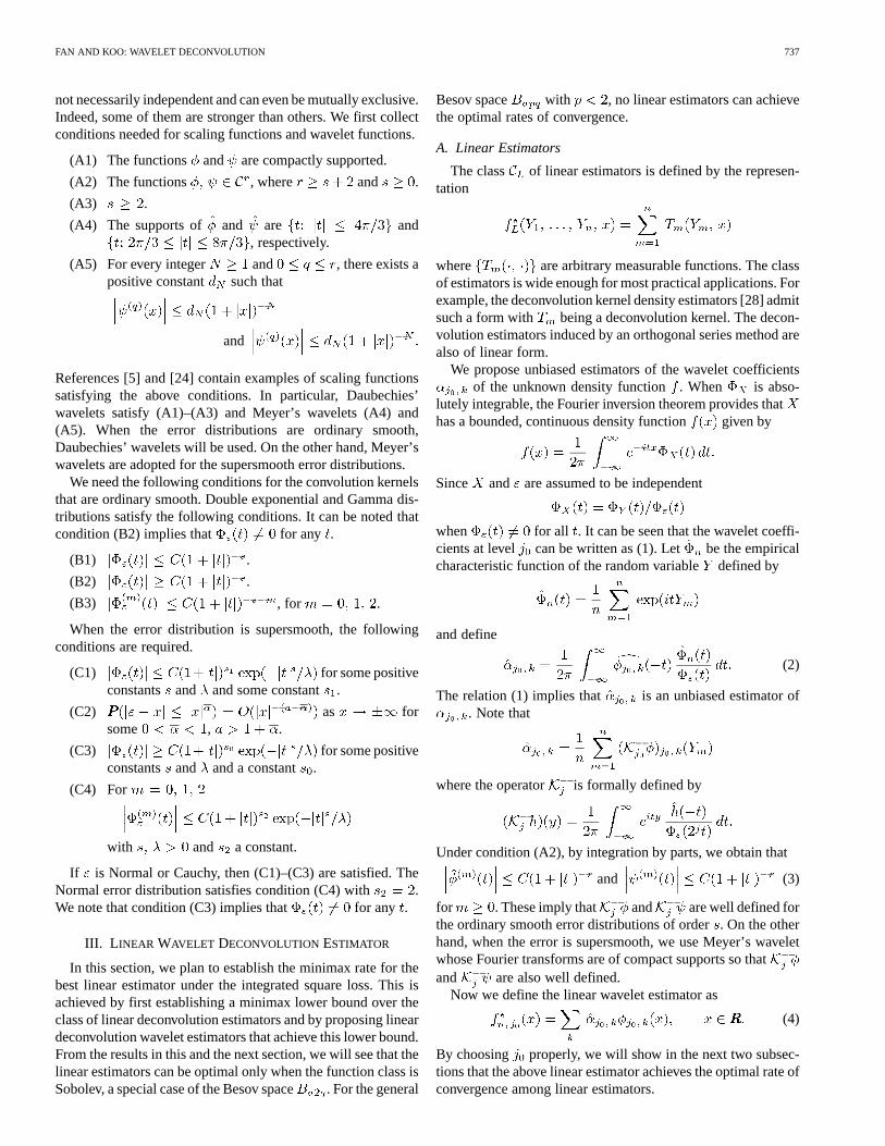
A. Linear Estimators
The class of linear estimators is defined by the represen-tation
where are arbitrary measurable functions. The classof estimators is wide enough for most practical applications. Forexample, the deconvolution kernel density estimators [28] admitsuch a form with being a deconvolution kernel. The decon-volution estimators induced by an orthogonal series method arealso of linear form.
We propose unbiased estimators of the wavelet coefficientsof the unknown density function. When is abso-
lutely integrable, the Fourier inversion theorem provides thathas a bounded, continuous density function given by
Since and are assumed to be independent
when for all . It can be seen that the wavelet coeffi-cients at level can be written as (1). Let be the empiricalcharacteristic function of the random variabledefined by
and define
(2)
The relation (1) implies that is an unbiased estimator of. Note that
where the operator is formally defined by
Under condition (A2), by integration by parts, we obtain that
and (3)
for . These imply that and are well defined forthe ordinary smooth error distributions of order. On the otherhand, when the error is supersmooth, we use Meyer’s waveletwhose Fourier transforms are of compact supports so thatand are also well defined.
Now we define the linear wavelet estimator as
(4)
By choosing properly, we will show in the next two subsec-tions that the above linear estimator achieves the optimal rate ofconvergence among linear estimators.

738 IEEE TRANSACTIONS ON INFORMATION THEORY, VOL. 48, NO. 3, MARCH 2002
B. Ordinary Smooth Case
Daubechies’ compactly supported wavelets satisfying (A1)–(A3) are employed for deconvolution with the ordinary smoothconvolution kernels. The following theorem states the best pos-sible rate for the class linear estimators when the convolutionkernel is ordinary smooth.
Theorem 1: Suppose that , , and .Then, under conditions (A1), (A2), and (B3), we have that
Since has compact support, the summation inof the linearwavelet deconvolution estimator (4) is finite for each .The following theorem shows that the lower bound on the linearestimators is achievable by linear wavelet estimators when theerror is ordinary smooth.
Theorem 2: Suppose that , , and .Under conditions (A1), (A2), and (B2), we have that
provided that . The result also holds for theclass under the additional conditions (A3) and(B3).
C. Supersmooth Case
For the supersmooth kernels, Meyer’s wavelets satisfying(A4) and (A5) are employed. The following theorems establishthe lower and the upper bounds. The optimal rates are only oflogarithmic order.
Theorem 3: If , , and , then, underconditions (A4), (A5), (C1), and (C2), we have that
Lemma 2 below implies that, for all
under the conditions (C1)–(C3). Hence, the linear waveletestimator is also well defined for the supersmoothcase. According to the following theorem, the lower bound onthe linear estimators is achievable by linear wavelet estimatorswhen the error is supersmooth.
Theorem 4: Suppose that , , and .Under the assumptions (A4), (A5), (C1)–(C3), we have that
provided that
The result also holds for the class under theadditional condition (C4).
D. Proof of Theorem 1
We first introduce a few lemmas before proving Theorem 1.Define the operator by
By Fourier inversion formula
(5)
where is the distribution function of the random variable.
Lemma 1: Under the assumptions (A2), (B3), we have
Proof: By (A2) and [5, Corollary 5.5.3]
for . From this and Taylor’s theorem we obtain
for (6)
as . It follows from (B3), (3), and (6) that
which implies that
for
Suppose . Let
By (B3)
as for
It follows from this and integration by parts that
Observing that
and using (3) and (6), we get that
from which the desired result follows.
Lemma 2 [30]: Suppose is a function on such that
Then for any sequence of scalars , we have that, for

FAN AND KOO: WAVELET DECONVOLUTION 739
Lemma 3: Under the assumptions (A2), (B3), we have thatfor any sequence of scalars
Proof: Observe that
By Lemma 1 and Lemma 2, we have the desired result.
Let
where is a constant such that is a density. Note that asgets close to , the constant is close to zero. Since isinfinitely differentiable, by choosing arbitrarily close towe may assume that
Consider the hypercube defined by
or
where and is a constant tobe specified later.
Lemma 4: Suppose that (A2) and (B3) hold. If can bechosen such that
(7)
then
for all .Proof: Let . By (7)
for all
from which it follows that
(8)
for all . Write
From (5) and Lemma 1
Note that the number of elements in is of order . Applying[13, Lemma 7] to the function
we have that
Hence, by [11, Lemma 5.1]
It follows from this and (8), we obtain the desired result.
To prove Theorem 1, we use the subclass of densitieswith
The constant will be chosen below. When , thefunctions
and
belong to , and the pyramid
for
is contained in .Suppose that is such that
for all and
We first use the information inequality to establish a lowerbound for the variance of the estimated wavelet coefficient
Let
By applying the information inequality of [20, Ch. 2, Theorem6.4] to the model in which is an independent andidentically distributed (i.i.d.) sample from forwith an unknown parameter , we have
where
Observe that
For fixed , is a fixed finite number de-pending only on the support of. Hence,
Choose in the definition of sufficiently small such that

740 IEEE TRANSACTIONS ON INFORMATION THEORY, VOL. 48, NO. 3, MARCH 2002
for sufficiently large. By the argument used to prove Lemma 4,we have
Thus,
(9)
We now follow arguments used to prove [8, Theorem 1] tocomplete the proof. Observe now that
and, hence,
By the definition of the pyramid
Note that
Using this, we have
(10)
Combination of (9) and (10) entails
The double sum is bounded from below by
Setting , we have
Recall that was constrained to be at most. This amountsto requiring that when is large, since
. To maximize the lower bound subject to this constraint,and should be of the same order. This leads
to choosing so that and, hence,
which establishes Theorem 1.
E. Proof of Theorem 2
Lemma 5: Under conditions (A2), (B2), we have
and
Proof: By (3), (A2), and (B2)
which is the desired result for . Since the same argumentcan be applied for , the proof is now complete.
Lemma 6: Suppose that conditions (A2), (A3), (B2), and(B3) hold. Then, we have
and
Proof: By Lemma 5
for
Suppose . Let
By (A2), (B2), (B3), and (3), as for. It follows from (3) and (A3) that
Hence, by integration by parts
Now let
It follows from (3) and (A3) that
This completes the proof since the same argument is truefor .
Now we prove Theorem 2. If , then

FAN AND KOO: WAVELET DECONVOLUTION 741
where and . Consequently, if, from which it follows that .
We now consider two cases.
a) Suppose that . Then, the number ofthat is not vanishing is only of order . Recall that
. By Lemma 5
from which it follows that
(11)
Using the fact that
(12)
Choose . Combination of (11) and(12) leads to
b) Consider the case when . Let
Observe that for any given
It follows from this and Lemma 6 that .Hence,
Now we obtain the desired result as in a). This completesthe proof of Theorem 2.
F. Proof of Theorem 3
The key idea of the proof is similar to that in the proof ofTheorem 1. We continue to use the notation introduced in theproof of Theorem 1.
Lemma 7: Suppose that conditions (A4) and (C1) hold. Then
Proof: By the Parseval identity and conditions (A4) and(C1)
This completes the proof.
Lemma 8: Assume that conditions (A5) and (C2) hold. Then,for
Proof: Choose in (A5) such that . By[11, Lemma 5.2] and (5), when
which is what needed to be shown.
Consider the hypercube defined by
or
Lemma 9: Suppose that (A4), (A5), (C1), (C2) hold. Ifcanbe chosen such that for , then we have
for all , where and.
Proof: Again, let and write
where . By Lemma 7
Let
and

742 IEEE TRANSACTIONS ON INFORMATION THEORY, VOL. 48, NO. 3, MARCH 2002
Observe that
Using [11, Lemma 5.1] and Lemma 7, we obtain that
It follows from [13, Lemma 7] and Lemma 8 that
(13)
for . By (13)
Combining the bounds on and , we have the desiredresult.
To complete the proof of Theorem 3, we consider the subclass. By (A5) and [13, Lemma 7], when and is large
which implies that for all . We nowfollow the arguments in the proof of Theorem 1 to complete theproof.
By the argument used in proving Lemma 9, we obtain that
for some . Hence,
Now, as in the proof of Theorem 1, we can show that
after setting
To maximize the lower bound subject to the constraint thatisat most , choose so that
with
Then
which establishes Theorem 3.
G. Proof of Theorem 4
Lemma 10: Under conditions (A4), (A5), (C3), we have
and
Proof: Let . Observe that
By (C3), when
(14)
and
when (15)
The conclusion follows directly from the above inequalities.
Lemma 11: Under conditions (A4), (A5), (C3)–(C4), wehave that, for some real constant
and
Proof: By (14), (15), the desired result follows as in Lem-ma 6.
If or , then . UsingLemma 10, we can prove the desired result for the case when
, as in Theorem 2. Now consider the case when. Let
It follows from this and Lemma 11 that
Hence,
by choosing the level such that
where if , and if . Hence, theterm

FAN AND KOO: WAVELET DECONVOLUTION 743
is negligible. Since
we have
from which the desired result follows.
IV. NONLINEAR WAVELET DECONVOLUTION ESTIMATOR
The aim of this section is to establish the minimax rate forestimating the density in . This is accomplished by firstestablishing a minimax lower bound and then showing that aclass of nonlinear wavelet deconvolution estimators achievesthe rate of the lower bound. For ordinary smooth convolutionkernels, we will show that thresholding wavelet deconvolutionestimators are optimal within a logarithmic order. However, forthe supersmooth case, since the optimal rates are only of loga-rithmic orders (see Theorems 3 and 7), losing a factor of log-arithmic orders in nonlinear wavelet deconvolution estimatorsmakes the thresholding wavelet estimators perform similarly tolinear wavelet estimators. Indeed, our study shows that the lastresolution level (see notation below) in thresholding waveletestimators has to be large enough in order to make approxi-mation errors negligible. Yet, this creates excessive variance inthe estimated wavelet coefficients at high resolution levels andhence the thresholding does not have much effect on the overallperformance of thresholding wavelet estimators. For this reason,we do not present the upper bound for the thresholding waveletestimators for the supersmooth case. Only lower bound is pre-sented to ensure that minimax rates for deconvolution with su-persmooth kernels are only of logarithmic orders.
A. Minimax Lower Bound
To establish minimax lower bounds, we follow the popularapproach, which consists of specifying a subproblem and usingFano’s lemma to calculate the difficulty of the subproblem. Thelower bound will then appear, where the Kullback–Leibler in-formation is crucial in using Fano’s lemma.
Let
and , the class of all estimators of based on .We have the following minimax lower bound for the ordinarysmooth error distributions.
Theorem 5: Suppose that and . Underconditions (A1)–(A3) and (B3), we have that
For supersmooth convolution kernels, we have shown (The-orems 3 and 4) that linear wavelet estimators have a very slowrate of convergence. Can they be improved significantly by othertypes of estimators? The following theorem shows that linear
wavelet estimators for the supersmooth case are optimal withina logarithmic order. As discussed at the beginning of this sec-tion, thresholding wavelet deconvolution estimators do not seemto enhance the performance, due to excessive variance of esti-mated wavelet coefficients at high resolution levels.
Theorem 6: Suppose that and . Underconditions (A4), (A5), (C1), (C2), we have that
B. Thresholding Wavelet Estimator
Among nonlinear estimators, we study a very special one: atruncated threshold wavelet estimator. Define
(16)
It can be seen that is an unbiased estimator of . Notethat
Define empirical wavelet coefficients and as in (2)and (16) and employ the hard-thresholding
ifif
where and the constant will be determined below.Then the nonlinear deconvolution wavelet estimator asso-ciated with the parameters , , and is
Take and such that
and
Theorem 7: Suppose that , , ,and . Then, under conditions (A1)–(A3),(B2), we have that there exist constantsand such that for
where .
The condition is purely a technical condi-tion. It was also imposed in [7].

744 IEEE TRANSACTIONS ON INFORMATION THEORY, VOL. 48, NO. 3, MARCH 2002
C. Proof of Theorem 5
Let , , and be the same as those defined in the proof ofTheorem 1. Consider the set of vertices of a hypercube definedby
with
Observe that
and that we can choose such that
for .Let denote the number of elements in the set. By [16,
Lemma 3.1] and the orthonormality of , there is a subsetof such that
for (17)
and
(18)
when is sufficiently large and .By Jensen’s inequality and Lemma 4, it can be seen that
(19)
for . By Fano’s lemma [2], [31], if is any estimatorof , then
(20)
Finally, let as . By (17), (18), andusing for some constant , the desired resultof Theorem 5 follows readily from (19) and (20).
D. Proof of Theorem 6
We use the same , except that is Meyer’s wavelet sat-isfying (A4) and (A5). As in the proof of Theorem 1, we cansee that for by choosing sufficientlysmall.
From the orthonormality of and [16, Lemma 3.1], (17)and (18) hold for the class , even when Meyer’s wavelets areused. By Jensen’s inequality and Lemma 9, it can be seen that
for . By Fano’s lemma, if is any estimator of ,then
Choosing such that
for a constant , we obtain the desired result of Theorem 6.
E. Proof of Theorem 7
In the first part, we set up the technical tools of the proof:moment bounds and large-deviation results. In the second part,we derive the results.
Moment Bounds:We use the result of [27]. Letbe i.i.d. random variables with , . Thenthere exists such that
if
if
Note that as it was shown in the proof of The-orem 2.
Recall that
and that
Applying Rosenthal’s inequality to
by Lemma 5
It follows that for
(21)
Large Deviation: We use the Bernstein’s or Bennett’s in-equality [26, pp. 192–193]. If are i.i.d. boundedrandom variables such that

FAN AND KOO: WAVELET DECONVOLUTION 745
then
Applying this to
and noting that, by Lemma 5, and
we conclude that if , then there exists a constantsuch that, for all
For example, it suffices to choose such that
We are ready to complete the proof. Write
where
Note that by the definition of
where .Using (12), we have
This bound has the rate of convergence specified in Theorem 7.By (21)
It follows that
This bound is the rate of convergence specified in Theorem 7.To decompose the details term, define
We may then write
For the term , we set
and
the large-deviation event. Clearly
Using this, and the Cauchy–Schwartz inequality and (21), wehave
Choosing , we have
Hence, it is negligible.To give a bound for , we note that
Hence,
by choosing . Hence, is at most of the specifiedrate of convergence.
To derive a bound on , let
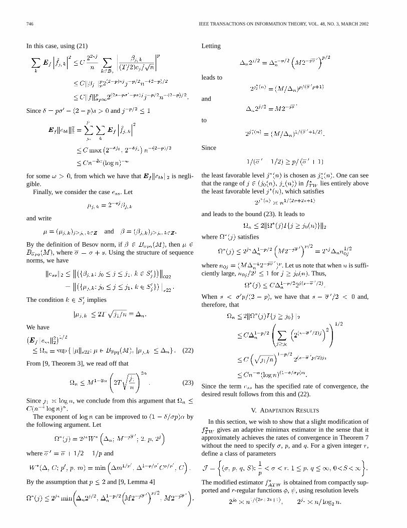
746 IEEE TRANSACTIONS ON INFORMATION THEORY, VOL. 48, NO. 3, MARCH 2002
In this case, using (21)
Since and
for some , from which we have that is negli-gible.
Finally, we consider the case . Let
and write
and
By the definition of Besov norm, if , then, where . Using the structure of sequence
norms, we have
The condition implies
We have
(22)
From [9, Theorem 3], we read off that
(23)
Since , we conclude from this argument that.
The exponent of can be improved to bythe following argument. Let
where and
By the assumption that and [9, Lemma 4]
Letting
leads to
and
to
Since
the least favorable level is chosen as . One can seethat the range of in lies entirely abovethe least favorable level , which satisfies
and leads to the bound (23). It leads to
where satisfies
where . Let us note that when is suffi-ciently large, for . Thus,
When , we have that and,therefore, that
Since the term has the specified rate of convergence, thedesired result follows from this and (22).
V. ADAPTATION RESULTS
In this section, we wish to show that a slight modification ofgives an adaptive minimax estimator in the sense that it
approximately achieves the rates of convergence in Theorem 7without the need to specify, , and . For a given integer,define a class of parameters
The modified estimator is obtained from compactly sup-ported and -regular functions , , using resolution levels
FAN AND KOO: WAVELET DECONVOLUTION 747
Theorem 8: Suppose that the conditions (A1)–(A3) and (B2)hold. If , where , then, forall , there exist andsuch that for
(24)
Proof: Because -norms decrease in for compactlysupported functions, the case reduces to the case .Thus, we investigate only the case . Define indexes
by
and
The indexes used in Theorem 7 are denoted by. Then
First of all, on , the rates of the bias and linearterms can easily be bounded as follows:
Secondly, the large-deviation terms and can be treatedexactly as for . The term is bounded by which issmaller than the bound in (24). For the term, by choosingsufficiently large
Therefore, it has the specified rate of convergence.We can establish the bound in Theorem 8 for the term.
For a bound on , we decompose
The term is bounded exactly as in the previous section. Forthe term , we have
Thus, the proof is completed.
ACKNOWLEDGMENT
Parts of this work were completed while J.-Y. Koo was vis-iting the Department of Statistics, University of North Carolina,Chapel-Hill, during summer 1999. He would like to take this op-portunity to thank the institution for its hospitality during thatvisit. The authors wish to thank an Associate Editor and the ref-erees who each made several helpful suggestions that improvedthe presentation and the results of the paper.
REFERENCES
[1] F. Abramovich and B. W. Silverman, “The vaguelette–wavelet decom-position approach to statistical inverse problems,”Biometrika, vol. 85,pp. 115–129, 1977.
[2] L. Birgé, “Approximation dans les espaces métriques et théorie de l’es-timation,” Z. Wahrsch. Verw. Geiete., vol. 65, pp. 181–237, 1983.
[3] R. J. Carroll and P. Hall, “Optimal rates of convergence for deconvolvinga density,”J. Amer. Statist. Assoc., vol. 83, pp. 1184–1186, 1988.
[4] R. J. Carroll, D. Ruppert, D. Stefanski, and L. A. Stefanski,MeasurementError in Nonlinear Models. London, U.K.: Chapman & Hall, 1995.
[5] I. Daubechies,Ten Lectures on Wavelets. Philadelphia, PA: SIAM,1992.
[6] P. J. Diggle and P. Hall, “A Fourier approach to nonparametric decon-volution of a density estimate,”J. Roy. Statist. Soc., ser. B, vol. 55, pp.523–531, 1993.
[7] D. L. Donoho, “Nonlinear solution of linear inverse problems bywavelet–vaguelette decomposition,”Appl. Comput. Harmonic Anal.,vol. 2, pp. 101–126, 1995.
[8] D. L. Donoho, I. M. Johnstone, G. Kerkyacharian, and D. Picard,“Density estimation by wavelet thresholding,”Ann. Statist., vol. 24, pp.508–539, 1996.
[9] , “Universal near minimaxity of wavelet shrinkage,” inFestschriftfür Lucien Le Cam, D. Pollard and G. Yang, Eds. Berlin, Germany:Springer-Verlag, 1997.
[10] S. Efromovich, “Density estimation for the case of supersmooth mea-surement error,”J. Amer. Statist. Assoc., vol. 92, pp. 526–535, 1997.
[11] J. Fan, “On the optimal rate of convergence for nonparametric deconvo-lution problems,”Ann. Statist., vol. 19, pp. 1257–1272, 1991.
[12] , “Adaptively local one-dimensional subproblems with applicationsto a deconvolution problem,”Ann. Statist., vol. 21, pp. 600–610, 1993.
[13] J. Fan and Y. K. Truong, “Nonparametric regression with errors in vari-ables,”Ann. Statist., vol. 21, pp. 1900–1925, 1993.
[14] N. W. Hengartner, “Adaptive demixing in Poisson mixture models,”Ann. Statist., vol. 25, pp. 917–928, 1997.
[15] E. D. Kolaczyk, “A wavelet shrinkage approach to tomographic imagereconstruction,”J. Amer. Statist. Assoc., vol. 91, pp. 1079–1090, 1996.
[16] J.-Y. Koo, “Optimal rates of convergence for nonparametric statisticalinverse problems,”Ann. Statist., vol. 21, pp. 590–599, 1993.
[17] , “Logspline deconvolution in Besov spaces,”Scand. J. Statist., vol.26, pp. 73–86, 1999.
[18] J.-Y. Koo and H.-Y. Chung, “Log-density estimation in linear inverseproblems,”Ann. Statist., vol. 26, pp. 335–362, 1998.
[19] J.-Y. Koo and B. U. Park, “B-spline deconvolution based on the EMalgorithm,”J. Statist. Comput. Simul., vol. 54, pp. 275–288, 1996.
[20] E. L. Lehmann,Theory of Point Estimation. Belmont, CA: Wadsworth,1991.
[21] M. C. Liu and R. L. Taylor, “A consistent nonparametric density esti-mator for the deconvolution problem,”Canad. J. Statist., vol. 17, pp.427–438, 1989.
[22] E. Masry, “Multivariate probability density deconvolution for sta-tionary random processes,”IEEE Trans. Inform. Theory, vol. 37, pp.1105–1115, July 1991.
[23] J. Mendelsohn and J. Rice, “Deconvolution of microfluorometric his-tograms with B-splines,”J. Amer. Statist. Assoc., vol. 77, pp. 748–753,1982.
[24] Y. Meyer, Wavelets and Operators. Cambridge, U.K.: CambridgeUniv. Press, 1992.
[25] M. Pensky and B. Vidakovic, “Adaptive wavelet estimator for nonpara-metric density deconvolution,”Ann. Statist., vol. 27, pp. 2033–2053,1998.
[26] D. Pollard,Convergence of Stochastic Processes. Berlin, Germany:Springer-Verlag, 1984.
[27] H. P. Rosenthal, “On the span inl of sequences of independent randomvariables,”Israel Math. J., vol. 8, pp. 273–303, 1972.
[28] L. Stefanski and R. J. Carroll, “Deconvoluting kernel density estima-tors,” Statistics, vol. 21, pp. 169–184, 1990.
[29] Y. Wang, “Function estimation via wavelet shrinkage for long-memorydata,”Ann. Statist., vol. 24, pp. 466–484, 1996.
[30] P. Wojtaszczyk,A Mathematical Introduction to Wavelets. Cambridge,U.K.: Cambridge Univ. Press, 1997.
[31] Y. G. Yatracos, “A lower bound on the error in nonparametric regressiontype problems,”Ann. Statist., vol. 16, pp. 1180–1187, 1988.
[32] C. H. Zhang, “Fourier methods for estimating mixing densities and dis-tributions,”Ann. Statist., vol. 18, pp. 806–831, 1990.


