Wave propagation and dynamic analysis of smoothly...

International Journal of Solids and Structures 44 (2007) 3601–3626

www.elsevier.com/locate/ijsolstr

Wave propagation and dynamic analysis of smoothlygraded heterogeneous continua using graded finite elements

Zhengyu (Jenny) Zhang, Glaucio H. Paulino *

Department of Civil and Environmental Engineering, University of Illinois at Urbana-Champaign, Newmark Laboratory,

205 North Mathews Avenue, Urbana, IL 61801, USA

Received 21 January 2005Available online 27 January 2007

Abstract

The dynamic behavior of smoothly graded heterogeneous materials is investigated using the finite element method. Theglobal variation of material properties (e.g., Young’s modulus, Poisson’s ratio and mass density) is treated at the elementlevel using a generalized isoparametric formulation. Three classes of examples are presented to illustrate this approach andto investigate the influence of material inhomogeneity on the characteristics of wave propagation pattern and stress redis-tribution. First, a cantilever beam example is presented for verification purposes. Emphasis is placed on the comparison ofnumerical results with analytical ones, as well as modal analysis for beams with different material gradation profiles. Sec-ond, wave propagation patterns are explored for a fixed-free slender bar considering homogeneous, bi-material, tri-layeredand smoothly graded materials (steel/alumina), which also provide further verification of the numerical procedures. Com-parison of stress histories in these samples indicates that the smooth transition of material gradation considerably alleviatesthe stress discontinuity in the bi-material system (with sharp interface). Third, a three-point-bending epoxy/glass gradedbeam specimen is investigated for validation purposes. The beam is graded along the height direction. Stress evolution his-tory at a location of interest is analyzed in detail, which not only reveals the dependence of stress evolution on materialgradation direction, but also provides information predictive of potential material failure time for graded beams with dif-ferent material gradation profiles. Jointly, these three classes of examples provide proper verification and validation for thepresent numerical techniques.� 2007 Elsevier Ltd. All rights reserved.

Keywords: Finite element method; Graded finite element; Graded material; Heterogeneous materials; Dynamic analysis; Wave propag-ation; Generalized isoparametric formulation

1. Introduction

Materials possessing smoothly graded properties have drawn increasing attention in material science andindustrial fields during the past decades due to their potential for providing improved performance inadvanced engineering applications (Paulino et al., 2003). They maybe designed as functionally graded

0020-7683/$ - see front matter � 2007 Elsevier Ltd. All rights reserved.

doi:10.1016/j.ijsolstr.2005.05.061

* Corresponding author. Tel.: +1 217 333 3817; fax: +1 217 265 8041.E-mail addresses: [email protected] (Z. Zhang), [email protected] (G.H. Paulino).

mailto:[email protected]

mailto:[email protected]

3602 Z. Zhang, G.H. Paulino / International Journal of Solids and Structures 44 (2007) 3601–3626

materials (FGMs) in which synthetic phases are graded to achieve desired properties and performance. Forexample, by smoothly interchanging the microstructural distribution of ceramic and metal phases in a gradedmaterial system, the resulting macro-structure takes advantage of desirable properties of both material con-stituents (e.g., hardness, corrosion resistance for ceramics and tensile strength, toughness for metals), and thusmakes itself an excellent candidate for thermal protection applications (Chin, 1999; Suresh and Mortensen,1998). Advanced material systems are frequently exposed to severe thermal/mechanical environments, andsubjected to dynamic and impact loadings. In order to enhance material/structural performance under variousdynamic loading conditions, it is essential to understand the system response and to identify critical instances(e.g., peak value of stress and failure initiation condition). Although a focus of academic and industrial inter-est, the dynamic behavior of this new generation of materials remains not well understood in relation tohomogeneous or standard composites (e.g., laminates). Non-homogeneity of the material system introducesconsiderable complexity in the boundary value problem and demands intense investigation to reveal the roleof material gradation on the system response. This work addresses some of the fundamental issues in the finiteelement modeling of graded material systems subjected to impact loading, and also investigates the influenceof material non-homogeneity on the dynamic response.

The literature on the dynamic response of graded material systems subjected to dynamic loading is lim-ited. The difficulty in obtaining analytical solutions for dynamic response of graded material systems iscompounded by the dispersive nature of the heterogeneous material system, which is characteristic of elas-todynamic response of material with continuously varying properties: ‘‘the pulse shape is distorted in time,the wave propagation speed is not constant, and there are no sharp interface that would cause wave reflec-tions’’ (Chiu and Erdogan, 1999). Therefore, analytical or semi-analytical solutions are available onlythrough a number of problems with simple boundary/initial conditions. Some problems with infinite/semi-infinite boundaries were solved using Laplace transforms. For instance, Whittier (1965) solved a slen-der bar with free–free ends and varying Young’s modulus, Payton (1966) considered a semi-infinite rodsubjected to a pressure step at its ends with several different wave speeds. Chiu and Erdogan (1999) solveda one-dimensional wave propagation in a functionally graded slab subjected to a pressure pulse with mate-rial gradation along the thickness direction. Their solution was obtained in wave summation form andthey provided an example, which shows that there is considerable wave distortion in time. Banks-Sillset al. (2002) have performed dynamic finite element analyses of FGMs (Al 6061-TO and TiC) using ADI-NA (Bathe, 1999). Their investigation included simulation of discrete micro-structure, layer modeling andconsideration of continuous change of material properties. Recently, Thamburaj et al. (2003) have imple-mented the damage model by Johnson and Holmquist (1994) into the dynamic finite element codeDYNA3D (Gazonas, 2002), and investigated the effect of graded strength on damage propagation in con-tinuously non-homogeneous materials. They observed that introducing different strength gradation canchange the location of site of maximum damage, which may have important implication in the designof impact resistant materials and structures.

The numerical study on dynamic response of graded materials has been an active research area of recently.Reddy and his co-workers (Praveen and Reddy, 1998; Reddy, 2000; Reddy and Chin, 1998) studied plates ofvarying material properties through thickness using shear deformation plate theories employing von Karmannon-linearity. Chakraborty and Gopalakrishnan (2003) developed the spectral finite element for wave analysisof functionally graded beams. Santare et al. (2003) compared the performance of both conventional andgraded elements in an elastic wave propagation problem and pointed out that in general, the graded elementoutperforms the homogeneous element in capturing the smooth transition of stress field across elementboundaries.

Few experimental data have been reported in literature for actual FGM specimens subjected to dynamicloading. Parameswaran and Shukla (1998, 2000) used photoelasticity technique to investigate dynamic frac-ture properties of a functionally graded material prepared by combining polyester resin and various amountof plasticizers. Rousseau and Tippur (2000, 2001a,b, 2002a,b) have conducted some dynamic experiments ofpolymer-based graded materials. These experimental data are employed in one of the simulations of this study,and our numerical results are compared with the experimental ones.

The remainder of this paper is organized as follows. First the temporal integration schemes used fordynamic analysis are described, followed by the graded element formulation for dynamic behavior of non-

Z. Zhang, G.H. Paulino / International Journal of Solids and Structures 44 (2007) 3601–3626 3603

homogeneous materials (Section 2). The numerical approach is both verified (i.e., the problem is solved cor-rectly in mathematical sense using the described numerical scheme) and validated, i.e., to demonstrate that theanalysis models the physical problem correctly by comparing the numerical solution with experimental obser-vations (see, for example, Roache (1998)). Three classes of problems are investigated. First, a cantilever beamsubjected to transverse transient point load is simulated to verify the numerical procedure by comparing theresults to those from analytical solution and modal analysis (Section 3). Second, the wave propagation pat-terns in fixed-free bars with different material variation types: homogenous, bi-material, tri-layered andgraded, are simulated to illustrate the relevance of material variation on the wave pattern (Section 4). Thisinvestigation provides further verification of the computational method. Third and finally, the stress evolutionhistory for a three-point-bending beam subjected to impact loading is studied for validation purposes (Section5). This investigation provides valuable insight on the prediction of structure bearing capacity (crack initia-tion) considering different material gradient cases. Finally, conclusions are inferred (Section 6).

2. Numerical scheme

In this section, the dynamic finite element formulation, the numerical aspects involving the dynamic updat-ing scheme and treatment of material non-homogeneity are presented. The two-dimensional dynamic finiteelement formulation can be derived from the principle of virtual work, which is expressed as
Z
Xðdivr� q€uÞdudX�

ZCðT� rnÞdudC ¼ 0 ð1Þ

where X represents domain area, C denotes boundary surface with normal vector n, u is the displacement vec-tor, T is the traction on the boundary, and r is the Cauchy stress tensor. The superposed dots (u) denote dif-ferentiation with respect to time, and q is the material density. By applying the divergence theorem andintegration by parts to the general expression in (1), the following conventional expression can be obtained:
Z
Xðr : dEþ q€u � duÞdX�

ZCext

Text � dudC ¼ 0 ð2Þ

where Cext represents the boundary surface on which external traction Text is applied, and E is the Green straintensor.

2.1. Dynamic updating scheme

Both implicit and explicit updating schemes can be adopted to investigate the dynamic wave propagationproblems. Usually implicit method is employed for long-term response analysis, while explicit method is pre-ferred for transient dynamic analysis. In this study, explicit method is employed to capture the transientresponse of the dynamic system. In addition, modal analysis is carried out in Section 3. The widely used New-mark b method is described by (Newmark, 1959):

M€unþ1 þ Kunþ1 ¼ Fnþ1 ð3Þ

unþ1 ¼ un þ Dt _un þDt2

2ð1� 2bÞ€un þ bDt2€unþ1 ð4Þ

_unþ1 ¼ _un þ ð1� cÞDt€un þ cDt€unþ1 ð5Þ

where Dt denotes the time step, M is the mass matrix, K is the stiffness matrix, F is the external force vector,and parameters b and c depend on the integration schemes employed. When b = 0, c = 1/2, the method be-comes the explicit method, or central difference method, which is conditionally stable with second order accu-racy. The explicit updating scheme for nodal displacements, accelerations and velocities from time step (n) to(n + 1) is given by the following expressions (see, for example, Hughes (1987))

Fig. 1.exampthe eleinterpo


unþ1 ¼ un þ Dt€un þ1

2Dt2€un ð6Þ

€unþ1 ¼M�1ðFnþ1 � Rintnþ1Þ ð7Þ

€unþ1 ¼ €un þDt2ð€un þ €unþ1Þ ð8Þ

where Rint is the internal force vector obtained from Rint = Ku.

2.2. Graded finite elements

To treat the material non-homogeneity inherent in the problem, we can use either homogeneous elementswith constant material properties at the element level, which are evaluated at the centroid of each element(Fig. 1(a)), or graded elements, which incorporate the material property gradient at the size scale of the ele-ment (Fig. 1(b)). Kim and Paulino (2002) and Santare and Lambros (2000) developed the graded element con-cept with slightly different formulations. Both studies demonstrated that graded elements result in smootherand more accurate results than homogeneous elements for static problems. In this study, the scheme developedby Kim and Paulino (2002) is extended to dynamic problems. It employs the same shape functions to inter-polate the unknown displacements, the geometry, and the material parameters, and hence assumes the nameGeneralized Isoparametric Formulation (GIF). The interpolations for spatial coordinates (x,y), displacements(u,v) and material properties (E,m,q) are given by

x ¼Xm

i¼1

N i xi; y ¼Xm

i¼1

N i yi ð9Þ

u ¼Xm

i¼1

N i ui; v ¼Xm

i¼1

N i vi ð10Þ

E ¼Xm

i¼1

Ni Ei; m ¼Xm

i¼1

N i mi; q ¼Xm

i¼1

N i qi ð11Þ

respectively, where Ni are the shape functions, and m is the number of nodes per element. The variations ofmaterial property, e.g., Young’s Modulus E, for homogeneous and graded elements are illustrated in Fig. 1.

By means of the principle of virtual work for the discretized finite element system, the element stiffnessmatrix and mass matrix are formulated as

0 0.1 0.2 0.3 0.4 0.5 0.6 0.7 0.8 0.9 10

0.5

1E

E

E (x)=E e1

1

2

βx

x=X/L

y=Y/H

E (

x)

0 0.1 0.2 0.3 0.4 0.5 0.6 0.7 0.8 0.9 10

0.5

1E1

E2

x=X/L

y=Y/H

E (

x)

iN E

iE(Gp)=Σ

βxE (x)=E1e

Material property at the element level (exponential gradation along the Cartesian x direction for Young’s modulus E is provided asle) – the symbols H and L denote height and length of a reference domain; (a) homogeneous element: material property evaluated atment centroid is used for the entire element; (b) graded element: material property is first evaluated at element nodes and thenlated to Gauss points (GP) using shape functions.


Ke ¼Z

XeBT CðxÞBdXe; Me ¼

ZXe

NT qðxÞNdXe ð12Þ

where B denotes spatial derivatives of the shape function matrix N, and C is the constitutive material matrix.The above mass matrix is formulated as consistent mass matrix. As indicated in the classical book by Hughes(1987), the transient integration scheme and mass matrices are ‘‘matched’’ so that the induced period errorstend to cancel. For example, the match can be trapezoidal rule and consistent mass, or central differencesand lumped mass. Therefore, in order to match the time integration scheme employed (central difference meth-od), lumped mass matrix is formulated such that only diagonal elements are preserved and scaled to maintainthe total mass:

Melump ¼ DiagðMe

consÞP

MeconsP

DiagðMeconsÞ

ð13Þ

where Melump and Me

cons stand for lumped and consistent mass matrices at the element level, respectively, andthe operator Diag(Æ) extracts the diagonal elements of a matrix.

A dynamic finite element code is developed, and both homogeneous and graded elements are implemented,however, for the reasons given above, graded elements are preferred. It is evident from Fig. 1(a) and (b) thatthe graded elements approximate the material gradation much closer to the original material profile, with asmooth transition across element boundaries, while the material distribution across homogeneous elementboundaries assumes a staircase-like profile. The use of graded elements is particularly beneficial within regionsof coarse mesh and/or with high stress gradient.

2.3. Wave speed and time step control in graded materials

The stability of conventional explicit finite element schemes is usually governed by the Courant condition(Bathe, 1996), which provides an upper limit for the size of the time step Dt:

Dt 6 ‘e=Cd ð14Þ
where ‘e is the shortest distance between two nodes in finite element mesh (Fig. 2), and the dilatational wavespeed Cd is expressed in terms of the material elastic constants E = E(x), m = m(x), and density q = q(x) as
C2dðxÞ ¼

EðxÞð1� mðxÞÞð1þ mðxÞÞð1� 2mðxÞÞqðxÞ : plane strain ð15Þ

C2dðxÞ ¼

EðxÞð1� m2ðxÞÞqðxÞ : plane stress: ð16Þ

The above expressions of dilatational wave speed assume linear elasticity. Because the problems under studyare restricted to linear elasticity, these expressions apply to the FEM formulation. However, since all materialproperties under consideration could vary in space, Cd is no longer a constant. To simplify the implementa-tion, the varying wave speed is calculated depending on the profile of the material property, and a uniformlimiting time step is used for the entire simulation.

Fig. 2. Illustration of shortest distance between nodes for computing Dt (Courant condition).


3. Verification: cantilever beam

In this section, the modal analysis of a cantilever beam is carried out, and its response under transient pointload is investigated for different material variation profiles. The results of this classical problem provide ver-ification of the numerical approach. They also reveal some interesting characteristics particular to a gradedcantilever beam.

First, the analytical solution for a homogeneous beam under transient point load is given. Next the Ray-leigh–Ritz method is employed to evaluate the influence of material gradation profile on the natural frequen-cies and modes of the structure. This result is further verified with FEM modal analysis, which reveals someinteresting features not captured by the standard one-dimensional (1D) Rayleigh–Ritz method. Finally, theresponses of graded beams of different material gradation profile are compared, which are in agreement withpredictions from the Rayleigh–Ritz method.

3.1. Problem description

Consider the cantilever beam illustrated by Fig. 3. The beam is of length L = 2 mm and height H = 0.1 mm(Fig. 3(a)). Transverse point load (Fig. 3(b)) is uniformly distributed along the free end of the beam, and con-sists of a sine pulse of duration T chosen as the period of the fundamental vibration mode of the cantileverbeam, i.e.,

T ¼ 2p=x1 ð17Þ

where x1 is the fundamental frequency of the beam.

3.1.1. Homogeneous beam

The natural frequencies xi of the cantilever beam are given by (see, e.g., Chopra (1995))

x2i ¼ k4

i

EIqA

; k1 ¼ 1:875=L; k2 ¼ 4:694=L; k3 ¼ 7:855=L; � � � ð18Þ

where E, q, I and A denote the beam elastic modulus, density, moment of inertia and cross-sectional area,respectively. Moreover, ki is a general dimensional parameter that bears the relationship given by Eq. (18).The analytical solution for the tip deflection is given by Warburton (1976)

uðL; tÞ ¼ 4PM

Xn

i¼1

1

xi

Z l

0

sinpsT

sin xiðt � sÞds

� �for 0 6 t 6 T

¼ 4PL3

EI

Xn

i¼1

p=ðxiT ÞðkiLÞ4ððp=xiT Þ2 � 1Þ

ðcos xiT þ 1Þ sin xiðt � T Þþ sin xiT cos xiðt � T Þ

� �" #for t P T

ð19Þ

0 0.2 0.4 0.6 0.8 1 1.2 1.4 1.6 1.8 2x 10

-3

2

1

0

1

2

3

4

5x 10

-4

P(t)

Y-C

oord

inat

e (m

)

X-Coordinate (m)0 0.2 0.4 0.6 0.8 1 1.2 1.4 1.6 1.8 2

0

0.2

0.4

0.6

0.8

1

t / T

P(t)

Fig. 3. (a) Geometry and FEM discretization (203 nodes, 80 T6 elements) of cantilever beam; (b) normalized load history.


where M = qA denotes the total mass of the beam. The T6 elements, with mesh discretization shown inFig. 3(a), produce very good results compared with the analytical solution expressed by Eq. (19), as demon-strated in Fig. 4, which shows that both results agree with plotting accuracy.

3.1.2. Graded beams

The material gradation for the graded cantilever beam (see Fig. 3) is considered along either x or y direction(Fig. 5). For each direction, three material gradation profiles are considered: exponential, linear and equiva-lent homogeneous, which can be expressed as follows (assume material properties vary in x direction).

For exponential material gradation

EðxÞ ¼ E1eax; qðxÞ ¼ q1ebx; mðxÞ ¼ m1ecx ð20Þ
where a, b and c are the material gradation parameters for E, q and m, respectively.
For linear material variation

EðxÞ ¼ E1 þ ðE2 � E1Þx=L

qðxÞ ¼ q1 þ ðq2 � q1Þx=L

mðxÞ ¼ m1 þ ðm2 � m1Þx=L

ð21Þ

where the subscripts 1 and 2 denote the two endpoints x = 0 and x = L, respectively.For equivalent homogeneous beam

E ¼ 1

A

ZEðxÞdA; q ¼ 1

A

ZqðxÞdA; m ¼ 1

A

ZmðxÞdA ð22Þ

which are defined as the equivalent material constants.

0 0.2 0.4 0.6 0.8 1 1.2 1.4 1.6 1.8 2

-0.5

-0.4

-0.3

-0.2

-0.1

0

0.1

0.2

0.3

0.4

0.5 AnalyticalFEM

t / T

u (t

) E

I

PL3

Fig. 4. Normalized displacement of homogeneous cantilever beam.

x

y

1 2

1

2

material gradation along x direction

material gradation along y directionx

y

Fig. 5. Beams with material gradation along the x and y directions, respectively.


3.2. Modal analysis

As the dynamic response of any system can be decomposed by combining its basic modes, the modal anal-ysis provides fundamental dynamic characteristics of the system. Two approaches are adopted to perform themodal analysis, the Rayleigh–Ritz method and the finite element method, and the results are compared.

3.2.1. Rayleigh–Ritz method

By simplifying the cantilever beam as a 1D problem with material variation along x direction, one obtainsthe governing equation

@2

@x2½EðxÞI @

2

@x2qðx; tÞ� þ qðxÞA @2

@t2qðx; tÞ ¼ f ðx; tÞ ð23Þ

where q(x, t) is the beam response under load f(x, t). To solve the eigenvalue problem, we set f(x, t) = 0, andconsider q(x, t) harmonic in time, i.e.,

qðx; tÞ ¼ uðxÞeixt ð24Þ

where x is frequency and u(x) is the corresponding mode shape. By introducing the energy conservation con-cept (Meirovitch, 1967), we obtain the Rayleigh’s quotient

RðuÞ ¼ x2 ¼R L

0 EðxÞI ½u00ðxÞ�2dxR L0 qðxÞAðuðxÞÞ2dx

¼ NðuÞDðuÞ : ð25Þ

If the function u chosen for expression (25) happens to be a true mode function, the frequency (x) solved forwill be the corresponding actual frequency. The stationarity of the Rayleigh quotient states that ‘‘the frequency

of vibration of a conservative system vibrating about an equilibrium position has a stationary value in the neigh-

borhood of a natural mode’’ (Meirovitch, 1967), hence we can construct trial mode functions and minimize theRayleigh’s quotient. A trial mode function can be constructed as

unðxÞ ¼Xn

i¼1

ai/iðxÞ

where ai are coefficients to be determined and /i are admissible functions that satisfy all the essential boundaryconditions

/ð0Þ ¼ 0; /0ð0Þ ¼ 0: ð26Þ

The necessary conditions for the minimum of the Rayleigh’s quotient are

@RðuÞ@aj

¼ 0; or@NðuÞ@aj

� k@DðuÞ@aj

¼ 0; j ¼ 1; 2; � � � ; n ð27Þ

where k is defined as the minimum estimated value of the Rayleigh’s quotient (Eq. (27)), i.e.,

minðRðuÞÞ ¼ k:

By introducing symmetric stiffness and mass matrices K and M:

Kij ¼Z l

0

EðxÞI @/iðxÞ@x

@/jðxÞ@x

dx; Mij ¼Z l

0

qðxÞA/iðxÞ/jðxÞdx; ð28Þ

N(u) and D(u) can be written in terms of these matrices as follows

NðuÞ ¼Xn

i¼1

Xn

j¼1

Kijaiaj; DðuÞ ¼Xn

i¼1

Xn

j¼1

Mijaiaj: ð29Þ

Introducing (29) into (27) and recalling the symmetry of the coefficients Kij, Mij, we obtain

TableNaturaRaylei

Num.

23456

Analyt

TableNaturaRaylei

Num.

23456

Analyt


Xn

j¼1

ðKrj � kMrjÞaj ¼ 0; r ¼ 1; 2; � � � ; n: ð30Þ

which represents a set of n homogeneous algebraic equations in the unknowns aj. Note that k = x2 render thelinear Eq. (30) into matrix form

K ¼ x2M ð31Þ
We can solve for the natural frequencies and corresponding modes, and the frequencies x provide upperbounds for the true frequencies x* (Meirovitch, 1967):
xr P x�r r ¼ 1; 2; � � � ; n ð32Þ
The base functions chosen for the graded cantilever beams under consideration are the polynomial series:
/1ðxÞ ¼ x2; /2ðxÞ ¼ x3; /3ðxÞ ¼ x4; /4ðxÞ ¼ x5 � � � ð33Þ
By incorporating more terms in the formulation, the Rayleigh–Ritz method guarantees that, with a completeset of base functions, the solution approaches the exact result asymptotically. The results listed in Tables 1–3are obtained for material properties
El ¼ 1 GPa; Eh ¼ 5 GPa; ql ¼ 0:5 g=cm3; qh ¼ 1:5 g=cm3 ð34Þ
where subscript l denotes the side where material elastic constants are lower, and h where it is higher.
In Tables 1–3, SoftLHS, StiffLHS and Equiv. denote the cases where the beam is softer (El,ql) at theclamped end, stiffer (Eh,qh) at the clamped end, and equivalent homogeneous beam as defined in Eq. (22).It is apparent that the beam which is softer at the clamped end has smaller natural frequency, and thus thewhole structure is more compliant than the case where the beam is stiffer at the clamped end. According toFig. 6, the equivalent homogeneous result is in between the other two, however, it is not simply the averageof the two. Moreover, the influence of the material gradation function (exponential and linear) is not as sig-nificant (cf. results from either Table 1, 2 or 3).

1l frequency x1 for graded beam and equivalent homogeneous beam considering gradation along x direction (obtained from

gh–Ritz method)

of base functions x1 (·104)

Exponential variation Linear variation

SoftLHS StiffLHS Equiv. SoftLHS StiffLHS Equiv.

2.7934 6.0983 4.2128 3.0405 6.2166 4.41592.6516 6.0705 4.1942 2.8388 6.2153 4.39632.6477 6.0673 4.1929 2.8183 6.2138 4.39502.2425 6.0666 4.1929 2.3823 6.2137 4.39502.2423 6.0655 4.1929 2.3816 6.2137 4.3950

ical – – 4.1929 – – 4.3950

2l frequency x2 for graded beam and equivalent homogeneous beam considering gradation along x direction (obtained from

gh–Ritz method)

of base functions x2 (·104)



46.479 36.856 41.508 47.063 38.972 43.50923.842 29.600 26.514 25.332 30.936 27.79222.428 29.140 26.424 23.837 30.785 27.69722.425 29.000 26.277 23.823 30.685 27.54422.423 28.971 26.277 23.816 30.675 27.543

ical – – 26.277 – – 27.543

Table 3Natural frequency x3 for graded beam and equivalent homogeneous beam considering gradation along x direction (obtained fromRayleigh–Ritz method)

Num. of base functions x3 (·104)



3 168.62 114.65 140.89 167.70 118.71 147.684 73.990 79.009 75.542 77.142 82.066 79.1835 69.346 76.547 75.414 72.671 80.779 79.0506 68.793 75.224 73.598 72.428 79.645 77.1457 68.680 74.948 73.596 72.415 79.521 77.1448 68.676 74.945 73.575 72.407 79.519 77.122

Analytical – – 73.580 – – 77.126

0 0.2 0.4 0.6 0.8 1 1.2 1.4 1.6 1.8 2x 10-3

0

5

10

15

20

25

30

35

40

45

50normalized first mode for graded cantilever beam

exponential, softLHSlinear, softLHS

exponential, stiffLHSlinear, stiffLHS

average property

x-Coordinate

v (x

)1

Fig. 6. Normalized 1st mode shapes of cantilever beams (Rayleigh–Ritz method).


The analytical solution for the equivalent homogeneous beams in Tables 1–3 are obtained by substitutingaveraged material properties (22) into Eq. (18). Clearly the Rayleigh–Ritz method gives excellent estimation oflower frequencies with only a few base functions for this case, and for FGM beams the frequencies also con-verge reasonably fast. However, for the higher modes we expect that more base function terms are needed.Since the Rayleigh–Ritz method is usually employed to obtain lower frequencies, the present study is limitedup to the 3rd mode.

The first two mode shapes of the structure are plotted in Figs. 6 and 7. The normalized mode shape isdefined as

viðxÞ ¼viðxÞffiffiffiffiffiffiffiffiffiffiffiffiffiffiffiffiffiffiffiffiffiR L

0v2

i ðxÞdxq ð35Þ

where vi(x) is the ith mode shape before normalization. The first mode is similar for all material gradationcases (Fig. 6), while for the higher mode the difference is more noticeable (Fig. 7). The Rayleigh–Ritz methodprovides better estimation of frequencies than mode shapes. We will reexamine the results by comparison withFEM results in the next section.

3.2.2. Comparison of modes from Rayleigh–Ritz and FEM

As an alternative approach to obtain the natural frequencies and modes, modal analysis is performed usingFEM. The global stiffness matrix K and mass matrix M are assembled, and boundary conditions are intro-duced. Then the following system is solved

0 0.2 0.4 0.6 0.8 1 1.2 1.4 1.6 1.8 2

x 10-3

-60

-50

-40

-30

-20

-10

0

10

20

30

40normalized second mode for graded cantilever beam

exponential, softLHS linear, softLHS

exponential, stiffLHSlinear, stiffLHS

average property

x Coordinate

v (x

)2

Fig. 7. Normalized 2nd mode shapes of cantilever beams (Rayleigh–Ritz method).

TableFirst s

x (·10

x1

x2

x3

x4

x5

x6


Ku� x2Mu ¼ 0: ð36Þ

Six natural frequencies are provided in Table 4 for graded beams and equivalent homogeneous beams, eachwith different material gradation profiles. The corresponding mode shapes are plotted in Figs. 8–10. Some con-clusions can be drawn from the results:

• Comparison of Table 4 and Tables 1–3 reveals that the results from the two methods (Rayleigh–Ritz andFEM) are in reasonably good agreement. Some of the differences are a consequence of modeling the 2Dstructure using a 1D model with the Rayleigh–Ritz method employed in the previous section. When a2D structure is simplified as a 1D model, the Poisson ratio effect is ignored.

• The trend of influence of material gradation on frequency is consistent with the conclusion from the Ray-leigh–Ritz method, i.e., the beams softer at the clamped end are more compliant than the beams stiffer atthe clamped end, thus producing smaller frequencies compared to the latter. For material gradation along y

direction, the results are close to those of the equivalent homogeneous beams.• The influence of material variation magnitude on frequency is more significant for the lower modes than for

higher modes. For example, for an exponentially graded beam under mode 1, the frequency for SoftLHS is 2.3times of that for StiffLHS (6.055/2.649 = 2.29), while at mode 6, the ratio is merely 1.029 (217.14/211.04).

A longitudinal vibration mode is found in the 2D FEM analysis. This mode occurs as 4th mode for both thebeam softer at the clamped end (Fig. 8(d)) and the equivalent homogeneous beam (not reported in the paper),while it occurs as 5th mode for the beam stiffer at the clamped end (Fig. 9(e)). This indicates that differentmaterial gradation profiles can change the sequence of some particular modes. A similar mode shape occursfor beams graded along y direction as 5th mode (Fig. 10), yet it is not purely elongation–compression along x

4ix natural frequencies (xi, i = 1, . . . , 6) for graded beams and equivalent homogeneous beam from FEM modal analysis

4) Exponential variation Linear variation

SoftLHS StiffLHS Y_grad Equiv. SoftLHS StiffLHS Y_grad Equiv.

2.649 6.055 3.882 4.190 2.816 6.204 4.055 4.39222.15 28.63 24.08 25.97 23.52 30.31 25.16 27.2266.70 72.83 66.38 71.51 70.31 77.25 69.39 74.9693.86 136.36 127.19 129.89 100.20 144.48 133.13 136.15

130.27 162.41 130.00 136.94 137.29 169.56 136.21 143.54211.04 217.14 205.04 220.16 222.47 229.82 214.70 230.77

0 0.2 0.4 0.6 0.8 1 1.2 1.4 1.6 1.8 2-2

0

2

x 10-4

x 10-4

X

Y

0 0.2 0.4 0.6 0.8 1 1.2 1.4 1.6 1.8 2-2

0

2x 10

-4

x 10-4

X

Y

0 0.2 0.4 0.6 0.8 1 1.2 1.4 1.6 1.8 2-2

0

2

x 10-4

x 10-4

X

Y

mode 2

0 0.2 0.4 0.6 0.8 1 1.2 1.4 1.6 1.8 2-2

0

2

x 10-4

x 10-4

X

Y

mode 4

0 0.2 0.4 0.6 0.8 1 1.2 1.4 1.6 1.8 2-2

0

2x 10

-4

x 10-4

X

Y

mode 3

0 0.2 0.4 0.6 0.8 1 1.2 1.4 1.6 1.8 2-2

0

2

x 10-4

x 10-4

X

Y

mode 1

mode 6mode 5

a b

c d

e f

Fig. 9. Six mode shapes of graded cantilever beam, linear gradation along x direction, stiffer at clamped end (StiffLHS), E2/E1 = 1/5,q2/q1 = 1/3.

0 0.2 0.4 0.6 0.8 1 1.2 1.4 1.6 1.8 2-2

0

2

x 10-4

x 10-4

X

Y

mode 1

0 0.2 0.4 0.6 0.8 1 1.2 1.4 1.6 1.8 2-2

0

2

x 10-4

x 10-4

X

Y

mode 2

0 0.2 0.4 0.6 0.8 1.2 1.4 1.6 1.8 2-2

0

2x 10

-4

x 10-4

X

Y

mode 4

0 0.2 0.4 0.6 0.8 1 1.2 1.4 1.6 1.8 2-2

0

2x 10

-4

x 10-4

X

Y

mode 3

0 0.2 0.4 0.6 0.8 1 1.2 1.4 1.6 1.8 2-2

0

2x 10

-4

x 10-4

X

Y

mode 5

0 0.2 0.4 0.6 0.8 1 1.2 1.4 1.6 1.8 2-2

0

2x 10

-4

x 10-4

X

Y

mode 6

1

a b

c d

e f

Fig. 8. Six mode shapes of graded cantilever beam, linear gradation along x direction, softer at clamped end (SoftLHS), E2/E1 = 5,q2/q1 = 3.


direction, but rather accompanied with bending in y direction (as expected). This behavior is induced by thenon-symmetric material distribution along the height direction of the beam, which prevents the beam fromdisplaying a deformation pattern purely along the x direction.

0 0.2 0.4 0.6 0.8 1 1.2 1.4 1.6 1.8 2-2

0

2x 10

-4

x 10-4

X

Y

mode 1

-2

0

2x 10

-4

Y

0 0.2 0.4 0.6 0.8 1 1.2 1.4 1.6 1.8 2x 10

-4X

mode 3

-2

0

2x 10

-4

Y

0 0.2 0.4 0.6 0.8 1.2 1.4 1.6 1.8 2x 10

-4X

mode 5

-2

0

2x 10

-4

Y

0 0.2 0.4 0.6 0.8 1 1.2 1.4 1.6 1.8 2x 10

-4X

mode 2

-2

0

2x 10

-4

Y

0 0.2 0.4 0.6 0.8 1 1.2 1.4 1.6 1.8 2x 10

-4X

mode 4

0

2x 10

-4

Y0 0.2 0.4 0.6 0.8 1.2 1.4 1.6 1.8 2

x 10-4

Xmode 6

-21 1

a b

c d

e f

Fig. 10. Six mode shapes of graded cantilever beam, linear gradation along y direction, E2/E1 = 5, q2/q1 = 3.


The Rayleigh–Ritz method performed in the previous section is unable to catch the longitudinal modeshape, since the polynomial base functions can only give rise to deformation in y direction. This is inherentto the base functions we choose, however, and the Rayleigh–Ritz method still proves to be remarkably efficientand accurate for obtaining the lower frequencies and mode shapes for graded beams.

3.3. Graded cantilever beams subjected to transient point load

Under the tip point load (Fig. 3(b)), where the period T is the fundamental period of each graded beam, theresponse of the cantilever beam is dominated by the first mode behavior. This can be clearly observed fromFig. 11, where all beam responses match the 1st natural frequency. At t > T, when transient force vanishes,the free vibration of each beam follows its own fundamental period, and its amplitude is scaled with respect

0 0.1 0.2 0.3 0.4 0.5 0.6 0.7 0.8 0.9 10

0.2

0.4

0.6

0.8

1

t / T

u(E av

gI)/P

L3 equivalent homog.

gradation along Y

stiff LHS

soft LHS

Normalized Tip Displacement

Fig. 11. Normalized tip displacement of graded cantilever beams under transient sine curve load (Fig. 3(b)). For the graded beams, thematerial changes linearly with modulus contrast of 5 and density contrast of 3.


to the amplitude at t < T in the same manner as the analytical solution in Fig. 4. The deflection amplitude ofbeams with different material gradations are in agreement with the observation in the previous section, i.e.,beam softer at the clamped end has larger deflection; beam stiffer at the clamped end has smaller deflection;beam graded along y direction and equivalent homogeneous beam are in between the other two, while beamgraded along y direction is more compliant than equivalent beam.

4. Verification: one-dimensional wave propagation

Transient wave propagation along a fixed-free bar is investigated considering homogeneous, bi-material,and graded material properties along the height direction. The objective of this example is to investigatethe influence of material gradation on the wave propagation pattern.


Consider the fixed-free slender bar illustrated in Fig. 12(a). The bar is of length L = 1 m, and heightH = 0.05 m. A transient axial loading with high frequency (Fig. 12(b)) is applied across the right free surfaceof the bar, which consists of a sine pulse of duration 50 ls. The fundamental period is T = 0.0174 s.

Four material gradation cases along the beam height are considered: homogeneous, bi-material, tri-layeredand smoothly graded, as shown in Fig. 13(a)–(d), respectively. The material system under consideration istaken as: steel for homogeneous bar, steel/alumina for both bi-material and graded bars. The material prop-erties for steel and alumina are provided in Table 5. For bi-material bar, the cross section is made of steel inthe upper half and alumina in the lower half, with a sharp interface in the middle. For the tri-layered bar, thecross section is made of steel in the upper layer, alumina in the lower layer, and smooth transition layer inbetween. For graded regions, material property varies linearly from pure steel at upper surface to pure alu-mina at lower surface.

4.2. Mesh size control

High order modes participate in the bar response of Fig. 12, which in turn requires refined element size(Chakraborty and Gopalakrishnan, 2003). To capture the transient response, the time step needs to be small

0.05m

F (t)

1m 0 50 100 150–0.2

0

0.2

0.4

0.6

0.8

1

t (μs)

F (

N)

Fig. 12. Geometry and applied force for a fixed-free thin bar; (a) geometry; (b) applied load history.

5mm SteelAlumina

2.5mm

2.5mm

Steel

Alumina

1mm Steel

3mm

1mm

Alumina

5mm

Steel

Fig. 13. Bar cross section material property; (a) homogeneous bar; (b) bi-material bar; (c) tri-layered bar; (d) graded bar.

Table 5Steel and alumina material properties

Material E (GPa) m q (kg/m3) Cd (m/s)

Steel 210 0.31 7800 6109Alumina 390 0.22 3950 10617


enough in order to track the change of applied load, and adequate element size can be estimated according tothe Courant condition. For example, when the applied force period is discretized into 100 time steps, the cor-responding element size is

h ¼ Cd � Dt ¼ 6109� 50� 10�6

100¼ 3:06� 10�3m ¼ 3:06 mm: ð37Þ

Taking into account material gradation along the height direction, the bar of Fig. 12(a) is discretized into300 · 15 quads, each divided into 4 T6 elements. This leads to a mesh with 36,631 nodes and 18,000 T6 ele-ments, which is used for the wave propagation problem.

4.3. Results and discussions

The analytical solution for a 1D stress wave propagation is given by Meirovitch (1967)

rðx; tÞ ¼ r0f t þ xCd

� �þ r0f t � x

Cd

� �ð38Þ

where the first and second term on the right hand side indicate the left-traveling-wave and the right-traveling-wave, respectively. The parameters r0 and r0 are the magnitude of the impact stress f(t), while the sign dependson the boundary condition where the wave impacts. When the stress wave reaches a fixed end, the stress mag-nitude doubles while the velocity changes sign; when the stress wave reaches a free end, the stress vanisheswhile the velocity doubles.

The numerical simulations employ 2D finite elements. Thus the current numerical model is not 1D in nat-ure, however it reasonably resembles a 1D case as the bar is slender. Therefore, we set the analytical solutionof the homogeneous bar as a reference result to which the numerical results are compared. Because the barsunder consideration possess different material properties, the results reported are normalized in order to pro-vide meaningful comparison. Therefore, stress is reported as r/r0 and time as t · Cd/L.

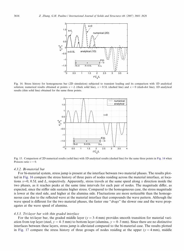
4.3.1. Homogeneous barIn 1D homogeneous case, the stress wave propagates at constant speed and retains its initial shape. This is

shown in Fig. 14. Three locations along the beam are chosen to represent the stress wave behavior. The freeend (x = L) experiences the stress wave which retains its shape, and afterwards this boundary becomes stress-free, as shown in Fig. 14 with the solid (x = L) curve. The stress wave travels across point x = 0.5L (dashcurve) at normalized time t 0 = t · Cd/L = 0.5, and impacts the fixed end point x = 0 (dash-dot curve) att 0 = 1, at which its magnitude is doubled. The wave reflects back, passes x = 0.5L position, and reaches thefree end at t 0 = 2. In the next cycle (normalized time t 0 = 2–4), the wave becomes compressive wave, and trav-els towards the fixed end and reflects back following similar pattern as described between normalized timet 0 = 0–2. The numerical result is also compared with the 1D analytical solution in Fig. 14. It is clearly shownthat the shape and magnitude of numerical results follow closely with the analytical solution. However, thereare small fluctuations in the 2D simulation which are absent from the 1D analytical solution. When Poissonratio m = 0, the problem becomes 1D and the upper and lower boundaries do not move. In the 2D simulation,as stress front propagates, the Poisson ratio effect results in constant vertical fluctuation of the upper andlower boundaries, which in turn induces fluctuation in stress wave. The difference in period is due to the neg-ligence of the Poisson ratio effect in the 1D analytical solution. To verify the above statement, another sim-ulation using Poisson ratio m = 0 is carried out. The amplitude and period of the numerical result matchesthe analytical solution, as shown in Fig. 15.

0 0.5 1 1.5 2 2.5 3 3.5 4–2

–1.5

–1

–0.5

0

0.5

1

1.5

2

t*Cd/L

σ x/σx0

numerical (2D)

analytical (1D)

x=L

x=0

x=0.5L

F(t)

X=0 X=LX=0.5L

Fig. 14. Stress history for homogeneous bar (2D simulation) subjected to transient loading and its comparison with 1D analyticalsolution; numerical results obtained at points x = L (thick solid line), x = 0.5L (dashed line) and x = 0 (dash-dot line); 1D analyticalresults (thin solid line) obtained for the same three points.

0 0.5 1 1.5 2 2.5 3 3.5 4–2

–1.5

–1

–0.5

0

0.5

1

1.5

2

t*Cd/L

σ x/σx0

numericalanalytical

ν=0

F(t)

X=0 X=LX=0.5L

Fig. 15. Comparison of 2D numerical results (solid line) with 1D analytical results (dashed line) for the same three points in Fig. 14 whenPoisson ratio m = 0.


4.3.2. Bi-material bar

For bi-material system, stress jump is present at the interface between two material phases. The results plot-ted in Fig. 16 compare the stress history of three pairs of nodes residing across the material interface, at loca-tions x=0, 0.5L and L, respectively. Apparently, stress travels at the same speed along x direction inside thetwo phases, as it reaches peaks at the same time intervals for each pair of nodes. The magnitude differ, asexpected, since the stiffer side sustains higher stress. Compared to the homogeneous case, the stress magnitudeis lower at the steel side, and higher at the alumina side. Fluctuations are more noticeable than the homoge-neous case due to the reflected wave at the material interface that compounds the wave pattern. Although thewave speed is different for the two material phases, the faster one ‘‘drags’’ the slower one and the wave prop-agates at the wave speed of alumina.

4.3.3. Tri-layer bar with thin graded interface

For the tri-layer bar, the graded middle layer (y = 3–4 mm) provides smooth transition for material vari-ation from top layer (steel, y = 4–5 mm) to bottom layer (alumina, y = 0–3 mm). Since there are no distinctiveinterfaces between these layers, stress jump is alleviated compared to the bi-material case. The results plottedin Fig. 17 compare the stress history of three groups of nodes residing at the upper (y = 4 mm), middle

0 0.5 1 1.5 2 2.5 3 3.5 4–2.5

–2

–1.5

–1

–0.5

0

0.5

1

1.5

2

2.5

t*(Cd)Alumina

/L

σ x/σx0

x=0, Alumina side

x=0, Steel side x=L, Steel side x=L, Alumina side

x=0.5L, Alumina side

x=0.5L, Steel side

F(t)

X=0 X=LX=0.5L

SteelAlumina

Fig. 16. Stress history of 6 points (indicated by solid dots in the insert) on a bi-material bar subjected to transient loading. Solid, dashed anddash-dot lines indicate points at x = L, 0.5L and 0, respectively. Thin and thick lines indicate points at alumina and steel side, respectively.

0 0.5 1 1.5 2 2.5 3 3.5 4–2.5

–2

–1.5

–1

–0.5

0

0.5

1

1.5

2

2.5

t*(Cd)Alumina

/L

σ x/σx0

x=L

x=0.5L

x=0 Alumina

Mid

Steel

F(t)

X=0 X=LX=0.5L

Graded

Steel

Alumina

Fig. 17. Stress history of 9 points (indicated by solid dots in the insert) on a tri-layer bar subjected to transient loading. Solid, dashed anddash-dot lines indicate points at x = L, 0.5L and 0, respectively. Thin, intermediate-thick and thick lines indicate alumina-rich side, mid-plane and steel-rich side of the graded interface, respectively.


(y = 3.5 mm) and lower (y = 3 mm) positions of the graded layer, at locations x=0, 0.5L and L, respectively.Apparently, stress travels at the same speed along x direction, and the stiffer side sustains higher stress.

4.3.4. Graded bar

Due to the gradual variation of material gradation, stress jump does not occur, but varies smoothly alongthe height direction. The results plotted in Fig. 18 compare the stress history of three groups of nodes residingat the upper, lower and middle surface, at locations x=0, 0.5L and L, respectively. Similarly to the bi-materialcase, the wave that moves fastest ‘‘drags’’ the rest to move along, so at the monitored points of same x loca-tion, the peak values occur simultaneously. At the free end, despite the material difference, the stress surgesacross the entire bar height with the same magnitude (since this is the initial boundary condition prescribed).The stress magnitude differ noticeably at other places, especially at the fixed end, where the alumina-rich sideexperience much higher stress than the opposite side. Also, the fluctuation is even more significant, due to thelarge number of wave tides that travel at different speeds.

4.3.5. Stress contour

Stress contours provide more instinctive image of the wave pattern. The stress distribution inside the bar atcertain time instant is shown for the three bars discussed above in Fig. 19. It clearly reveals a stress jump along

0 0.5 1 1.5 2 2.5 3 3.5 4–4

–3

–2

–1

0

1

2

3

4

t*(Cd)Alumina

/L

σ x/σx0

x=0

x=0.5L x=L

Alumina Mid

Steel

F (t)

X=0 X=LX=0.5L

Steel

Alumina

Fig. 18. Stress history of 9 points (indicated by solid dots in the insert) on a graded beam subjected to transient loading. Solid, dashed anddash-dot lines indicate points at x = L, 0.5L and 0, respectively. Thin, intermediate-thick and thick lines indicate alumina-rich side, mid-plane and steel-rich side, respectively.

Fig. 19. Comparison of stress contours (Pa) of the four bars; (a) homogeneous; (b) bi-material; (c) tri-layer; (d) smoothly graded.


material interface in the bi-material bar, while a smooth distribution of stress is achieved for the graded barand tri-layer bar.

With the above observation, we conclude that the material variation has strong influence of the wave pat-tern. The stress front travels at the speed of the stiffest material, and the stress peak at the stiffer material sidecan be remarkably higher than the homogeneous case if linear elastic behavior is considered and there is noother source of inelasticity. For example, for the smoothly graded case, the highest stress at the alumina sidereaches about 4 times the applied impact traction magnitude.

5. Validation: three-point-bending beams subjected to impact load

This section investigates the influence of material gradation profile on the evolution of stress state, via sim-ulation of a three-point-bending specimen under impact loading, which is based on a real material system. Thebeam is made of glass/epoxy phases. The experiments on material properties and dynamic fracture behavior ofthis graded specimen have been conducted by Rousseau and Tippur (2000, 2001a,b, 2002a,b). This study offersbackground knowledge of the dynamic behavior of this material system, as well as a sound understanding of


the stress field in homogeneous and graded materials, which helps to predict the fracture initiation time inspecimens of various material gradients.


The three-point-bending specimen under impact loading is illustrated in Fig. 20(a). Due to the symmetry ofgeometry, material gradation along the y direction and boundary condition, only half of the geometry is mod-eled for numerical analysis, as shown in Fig. 20(b). The mesh of the uncracked beam problem is plotted inFig. 21, which is also used for further investigation of fracture behavior using cohesive zone elements (Zhangand Paulino, 2005). The mesh is refined along the center line with uniform element size h = 92.5 lm, and thestress variation versus time is retrieved at point P, with coordinates (x,y) = (0,0.2W), where W is the height ofthe beam. The point P is of special interest because it corresponds to the crack tip location in other investi-gations of fracture behavior (Zhang and Paulino, 2005). Hence, the location of interest in this study corre-sponds to the crack tip location when the crack is present.

V =5m/sE2

E1

L=152mm

W=37mm

x

y

0 V =5m/s

E1

L=76mm

W=37mm

x

y

E20

P 0.2W

Fig. 20. Epoxy/glass beam subjected to point impact loading; (a) three-point-bending specimen with material gradation along they-direction; (b) half model with symmetric boundary conditions prescribed. Stress values are retrieved at point P: (x,y) = (0,0.2W).

x (m)

y(m

)

0 0.005 0.010

0.001

0.002

0.003

0.004

0.005

x (m)

y(m

)

0 0.02 0.04 0.060

0.01

0.02

0.03

0.037

0.076

Fig. 21. Discretization of half of the three-point-bending beam model. Mesh contains 7562 nodes and 3647 T6 elements; (a) global mesh;(b) zoom of box region in (a).


5.2. Material gradation

Three simulations are performed considering the following beam configurations under plane stressconditions:

• homogeneous beam (E2 = E1)• graded beam stiffer at the impacted surface (E2 > E1)• graded beam more compliant at the impacted surface (E2 < E1)

where subscripts 1 and 2 denote bottom and top surface, respectively. Fig. 22 shows the linear variation ofYoung’s modulus E and mass density q for the above three cases. The range of variation is between 4–12 GPa for E, and 1000–2000 kg/m3 for q, which approximates the range of the actual graded specimen mate-rial (Rousseau and Tippur, 2002a,b). For the homogeneous beam, the mass density is taken as the mean valueof the graded beam counterpart, i.e., 1500 kg/m3, and the Young’s modulus is calculated such that the equiv-alent E/q value equals that of the graded specimen case in an average sense, i.e.,

Fig. 22q and

Eq

� �equiv

¼ 1

W

Z W

0

EðyÞqðyÞ dy; ð39Þ

as shown in Fig. 23(a). Thus, the approach from Eq. (39) explains the offset observed in Fig. 22(a) for thehomogeneous material modulus (E1 = E2). Notice that although E and q are linear functions of y, the ratio

0 10 20 304

6

8

10

12

y (mm)

E (

GP

a)

0 10 20 301000

1200

1400

1600

1800

2000

y (mm)

(kg/

m3)

E2<E

1 E

2>E

1

E2=E1

E2<E

1 E

2>E

1

E2=E

1

. Variation of (a) Young’s modulus E and (b) mass density q in homogeneous and graded beams along y direction. The variation ofE are approximated from those provided in Figs. 1 and 2, respectively, of the reference by Rousseau and Tippur (2002b).

0 5 10 15 20 25 30 354

4.5

5

5.5

6x 106

y (mm)

E/

(m2 /s

2 )

E2<E

1 E

2>E

1

E2=E

1

0 5 10 15 20 25 30 35

2150

2200

2250

2300

2350

2400

2450

2500

2550

y (mm)

Cd (

m/s

)

E2>E

1 E

2<E

1

E2=E

1

avg (FGM)

ρ

Fig. 23. Variation of (a) E/q versus y and (b) dilatational wave speed Cd versus y in homogeneous and graded beams.


E/q is not. Poisson’s ratio is taken as 0.33 (constant) in all cases. The average dilatational wave speeds (Cd) isdefined as

Fig. 24point i

Fig. 25point i

ðCdÞavg ¼1

W

Z W

0

CdðyÞdy;

and the difference for each case is marginal (2421.5 m/s for homogeneous beam, 2418.4 m/s for graded beam,plotted in Fig. 23(b)).

5.3. Results and discussions

When the impact loading is applied at the top surface of the beam, stress waves are generated and propa-gate towards the lower surface and reflect back at the boundaries. A detailed stress history analysis is helpfulto characterize the stress wave behavior accounting for different material gradation profile cases, and also toprovide relevant information for predicting beam load bearing capacities. In this section, first the stress resultsare presented, and then their implication on behavior is discussed, which is facilitated by a statics beam theoryanalogy. The results for different material profiles are plotted in Figs. 24 and 25 for variation of rx and ry

versus normalized time, respectively.

0 1 2 3 4 5 6–2

0

2

4

6

8

10

12

14

16

t Cd(avg)

/W

σ x(MP

a)

E2/E

1=1

E2/E

1>1

E2/E

1<1

5m/sE2

E1

0.2WWP

. Stress rx at location P: (x,y) = (0,0.2W) in homogeneous and graded beams, with linearly varying elastic moduli, subjected to onempact by a rigid projectile.

0 1 2 3 4 5 6–3

–2.5

–2

–1.5

–1

–0.5

0

0.5

1

t Cd(avg)

/W

σ y(MP

a)

E2/E

1=1

E2/E

1>1

E2/E

1<1

0.8 1.2 2.8 3.2

5m/sE2

E1

0.2WWP

. Stress ry at location P: (x,y) = (0,0.2W) in homogeneous and graded beams, with linearly varying elastic moduli, subjected to onempact by a rigid projectile.


5.3.1. On the stress component rx

Fig. 24 indicates that stress component rx is primarily dominated by the bending effect. The location ofinterest (point P in Fig. 20(b)) first experiences stress wave at normalized time 0.8 because the time neededfor the first wave front to reach this point is 0.8W/Cd. This value is exact for homogeneous beam, whilefor the graded beam, the normalized time is slightly less than 0.8 for the E2 > E1 case, and slightly larger than0.8 for the E2 < E1 case. This is due to the effect of material gradation within the span of the top surface to thelocation of interest. The difference, though moderate, can be discerned in stress plots of Fig. 24. At this point(normalized time = 0.8), rx becomes negative (during normalized time period 0.8–1.3) due to Poission ratioeffect, however, this is quickly counterbalanced by the bending effect, and afterwards the stress value increasesmonotonically with respect to time. Point P in the beam with E2/E1 > 1 experiences higher tensile stress than inthe other two cases.

5.3.2. On the stress component ry

The stress component ry in Fig. 25 shows strong influence of waves traveling along y direction. The initialstages of this plot can be explained by the dominance of the first batch of propagating waves. At normalizedtime 0.8, the first tide of compressive wave brings a sharp increase of ry in magnitude, as compressive stress.The magnitude of ry increases as the subsequent tide of compressive waves pass through point P, till they passthis point again, as tensile wave, after being reflected from the bottom surface at normalized time 1.0. Thearrival of the tensile wave at this location, at normalized time 1.2, brings a sharp change of the stress profiletowards the opposite direction (magnitude decreases). This trend is sustained for a while till normalized time2.0, after which the combined effect of subsequent tensile waves that bounced back from the bottom surface,and the compressive waves emanated from the velocity loading, reaches certain balance level at this location,and a ‘‘plateau’’ can be observed from normalized time 2.0–2.8. At normalized time 2.8, the very first tide ofstress wave, after being reflected from top surface, again passes through point P, and another cycle of increase–

decrease in magnitude of ry can be observed during normalized time period 2.8–3.2, which is similar to that oftime interval 0.8–1.2. Afterwards, the combined effect of the numerous wave tides clouds the influence of anyisolated wave, and thus it is difficult to detect the precise time when the ry curve changes its trend. Further-more, waves that traveled to the lateral boundaries also bounce back, adding more complexity to the stressstate.

5.3.3. Crack initiation argument

As the load keep increasing, higher stress state in the beam may lead to microcrack and macrocrackformation and finally system failure. Although this study is confined to elastodynamic analysis withoutconsidering fracture behaviors, the stress evolution history provides insight on crack initiation character-istics for the three beams described above, through examination of the effect of material gradation onstress levels.

Fig. 26 shows the stress contours for different beams. The region close to the impact loading experiencescompressive rx, and the central bottom part of the beam experiences tensile rx. However, the stress contourpatterns are distinctively different for different material gradient cases. First, we notice that close to the topsurface, region of compressive rx is larger and spans much wider region along x direction for beam withE2 > E1, compared to homogeneous beam (cf. Fig. 26(c) and (b)), and is mostly constricted for beamwith E2 < E1 (Fig. 26(a)). This is due to the difference in material stiffness at the loaded region. For beam withE2 < E1, the material is soft under the point load, thus the beam deforms locally and the severe deformation isconstricted within a relatively small region. Consequently, the compressive stress region is constricted. Forbeam with E2 > E1, the material is relatively rigid under the point load, hence the deformation is sustainedby nearby region also. Therefore, a larger compressive stress region is developed for beam with E2 > E1 thanthat for beam with E2 < E1.

On the other hand, the rx value at the central bottom region, being far from the point loading, is dominatedby the bending effect. The tensile stress region is larger in the beam with E2 > E1 than the two other cases, dueto different position of neutral axis in each case. To understand the difference in tensile rx distribution patternsin the three beams, we resort to first examine a simpler and well-understood problem – a beam subjected tostatic uniform bending, e.g., the central region of four-point-bending beam.

Fig. 26. Effect of material gradient on the contour plot of stress field rx for data obtained at time t = 90 ls (legend shows rx value inMPa). (a) FGM beam with E2 < E1; (b) homogeneous beam; (c) FGM beam with E2 > E1.


5.3.4. Statics argument

Consider the stress distribution along y direction in the static case. By enforcing the equilibrium conditions,i.e.,

N ¼Z W

0

rxðyÞdy ¼ 0; M ¼Z W

0

rxðyÞydy;

location of neutral axis can be obtained. In the above expressions, N denotes the summation of normal trac-tion along the beam cross section, and M is the bending moment acting on the cross section of beam. For thehomogeneous beam, the neutral axis is located at half height of the beam. For the beam with E2 < E1, the


material is stiffer at the bottom part, and thus the neutral axis shifts towards the bottom. The opposite situ-ation applies to the beam with E2 > E1. This speculation can be confirmed by mathematical derivation. A sim-ple calculation reveals that the neutral axis is located at

y ¼ 0:415W ; for E2 < E1; y ¼ 0:585W ; for E2 > E1

for the material gradient considered (Fig. 22). Hence, a larger tensile stress region develops in beam with softermaterial at bottom (E2 > E1). At the location of interest, the tensile stress is higher for the beam with E2 < E1

than that for the beam with E2 > E1. A simple calculation is carried out here. Assume strain �2 = 0.01 at topsurface. In linear elastic beam with E2 > E1, the corresponding strain at the bottom surface is �1 = (0.585W/0.415W) · 0.01 = 0.014097. At location P: (x,y = 0,0.2W), rx can be obtained as rx(P) = E(P)�(P) = 51.96 M-Pa. For the beam with E2 < E1, with the same assumption of �2 = 0.01 at top surface, �1 = (0.415W/0.585W) · 0.01 = 0.007094 at the bottom surface. At location P: (x,y = 0,0.2W), rx is obtained asrx(P) = E(P)�(P) = 38.22 MPa.

5.3.5. Statics versus dynamicsThe above argument, though made for static analysis of linear elastic beam subjected to uniform bending,

provides an useful analogy for understanding the dynamic problem for beam under point loading. For a beamsubjected to point load, the compressive strain at the top surface is localized under the point load, while thetensile strain develops in a relatively larger region at bottom. The localization of compressive region shifts theneutral axis towards the top surface, as shown in the homogeneous case in Fig. 26(b). Compared to the homo-geneous beam, the neutral axis further shifts towards the top surface for FGM beam with E2 > E1, and shiftstowards the bottom surface for FGM beam with E2 < E1 (cf.Fig. 26(a) and (c) with (b)). This observation isconsistent with that made for the static uniform bending beam problem.

5.3.6. Closing remarkThe dynamic nature of the problem adds more difficulty to a precise prediction of the stress distribution at

certain time, as the neutral axis shifts with respect to time. However, at any specified time, the overall stressdistributions in the three beams are similar to those shown in Fig. 26. The above observation implies that thelocation of interest in the FGM beam with E2 > E1 is consistently subjected to higher tensile stress than itscounterparts. Since the crack initiation is primarily dominated by rx, crack initiation would be expected tooccur earlier for beam with E2 > E1. This is confirmed by both the experiment (Rousseau and Tippur,2002a) and the simulation carried out for fracture analysis (Zhang and Paulino, 2005). It needs to be pointedout, however, that this conclusion assumes identical fracture toughness at the crack tip for the three speci-mens, which is not true. Fracture toughness depends on local material compositions, which are clearly differ-ent for the three cases. This mechanism is considered in the fracture simulation, and the result proves to beconsistent with the predictions.

6. Conclusions

This work provides a thorough investigation of wave propagation behavior in smoothly graded heteroge-neous material systems considering different material variation profiles. Generalized isoparametric formula-tion is employed in 2D finite element method to investigate the response of graded material systems underdynamic loading. This formulation adopts the same interpolation methods of the coordinates and displace-ment to treat material inhomogeneity at the element level. This approach effectively represents the materialvariation at the element level and results in smooth solution transition across the element boundaries. Explicitupdating scheme is adopted to capture the transient response of the material systems under study. With thisapproach, three classes of problems are examined, including both verification and validation procedures.

Verification procedure is carried out through numerical example of a cantilever beam. Analytical solutionfor homogeneous problem is employed as reference result to verify the numerical approach. Next, beams withmaterial variation along either x or y directions are investigated. Both Rayleigh–Ritz method and FEM areemployed to study the influence of material variation on the fundamental modes and frequencies of the can-tilever beam. Results indicate some characteristics particular to the graded material system, including change


of the order of certain modes for different material variation profiles. Moreover, comparison of Rayleigh–Ritzmethod and FEM results reveals that by simplifying the 2D problem as a 1D model, modes in longitudinaldirection is ignored, and may result in a stiffer model.

The second class of problems, which also provides further verification of the computation procedure, con-sists of investigating wave propagation patterns in fixed-free bars considering homogeneous, bi-material, tri-layered and smoothly graded material profiles, respectively. In bi-material, tri-layered and smoothly gradedmaterial beams, wave propagates at the wave speed of the stiffer material, and the stress is much higher atthe stiffer side. Moreover, stress history reveals that graded material systems eliminate the stress mismatchpresent at the sharp bi-material interface. This class of problems also indicate the need for inelastic analysis,which is a topic that deserves further investigation (Zhang and Paulino, 2005).

The validation procedure is performed through simulation of a three-point-bending beam under impactloading, based on real epoxy/glass FGM beam experiment. The numerical results indicate that the tensilestress at location of interest develops at a faster rate for certain material gradation profile (E2 > E1) thanthe other cases. This trend is consistent with the experiment observation, and provides important informationfor predicting structure performance capacity, e.g., crack initiation. The fracture behavior for the polymer-based graded beam has been investigated by the authors (Zhang and Paulino, 2005) using cohesive zoneapproach, which proves to be consistent with the prediction in the current study.

References

Banks-Sills, L., Eliasi, R., Berlin, Y., 2002. Modeling of functionally graded materials in dynamic analysis. Composites B 33, 7–15.Bathe, K.-J., 1996. Finite Element Procedures. Prentice-Hall, New Jersey.Bathe, K.-J., 1999. ADINA-automatic dynamic incremental nonlinear analysis system, Version 7.3, Adina Engineering, Inc. USA.Chakraborty, A., Gopalakrishnan, J., 2003. A spectrally formulated finite element for wave propagation analysis in functionally graded

beams. International Journal of Solids and Structures 40, 2421–2448.Chin, E.S.C., 1999. Army focused research team on functionally graded armor composites. Materials Science and Engineering A259, 155–

161.Chiu, T.-C., Erdogan, F., 1999. One-dimensional wave propagation in a functionally graded elastic medium. Journal of Sound and

Vibration 222, 453–487.Chopra, A.K., 1995. Dynamics of Structures. Prentice-Hall, New Jersey.Gazonas, G.A., 2002. Implementation of the Johnson-Holmquist II (JH2) constitutive model into DYNA3D, ARL-TR-2699. Army

Research Laboratory, Aberdeen, MD.Hughes, T.J.R., 1987. The Finite Element Method: Linear Static and Dynamic Finite Element Analysis. Prentice Hall, New Jersey.Johnson, G.R., Holmquist, T.J., 1994. An improved computational model for brittle materials. In: Schmidt, S.C., Shaner, J.W., Samara,

G.A., Ross, M. (Eds.), High Pressure Science and Technology. American Institute of Physics Press, New York, pp. 981–984.Kim, J.-H., Paulino, G.H., 2002. Isoparametric graded finite elements for nonhomogeneous isotropic and orthotropic materials. ASME

Journal of Applied Mechanics 69, 502–514.Meirovitch, L., 1967. Analytical Methods in Vibrations. The Macmillan Company, New York.Newmark, N.M., 1959. A method of computation for structural dynamics. ASCE Journal of the Engineering Mechanics Division 85, 67–

94.Parameswaran, V., Shukla, A., 1998. Dynamic fracture of a functionally gradient material having discrete property variations. Journal of

Materials Science 33, 3303–3311.Parameswaran, V., Shukla, A., 2000. Processing and characterization of a model functionally gradient material. Journal of Materials

Science 35, 21–29.Paulino, G.H., Jin, Z.-H., Dodds Jr., R.H., 2003. Failure of Functionally Graded Materials. In: Karihaloo, B. et al. (Eds.), . In:

Encyclopedia of Comprehensive Structural Integrity, vol. 2. Elsevier, Amsterdam, pp. 607–644.Payton, R.G., 1966. Elastic wave propagation in a non-homogeneous rod. The Quarterly Journal of Mechanics and Applied Mathematics

19, 83–91.Praveen, G.N., Reddy, J.N., 1998. Nonlinear transient thermoelastic analysis of functionally graded ceramic-metal plates. International

Journal of Solids and Structures 35, 4457–4476.Reddy, J.N., 2000. Analysis of functionally graded plates. International Journal for Numerical Methods in Engineering 47, 663–684.Reddy, J.N., Chin, C.D., 1998. Thermomechanical analysis of functionally graded cylinders and plates. Journal of Thermal Stresses 26,

593–626.Roache, P.J., 1998. Verification and Validation in Computational Science and Engineering. Hermosa Publishers, Albuquerque, NM.Rousseau, C.-E., Tippur, H.V., 2000. Compositionally graded materials with cracks normal to the elastic gradient. Acta Materialia 48,

4021–4033.Rousseau, C.-E., Tippur, H.V., 2001a. Dynamic fracture of compositionally graded materials with cracks along the elastic gradient:

experiments and analysis. Mechanics of Materials 33, 403–421.


Rousseau, C.-E., Tippur, H.V., 2001b. Influence of elastic gradient profiles on dynamically loaded functionally graded materials: cracksalong the gradient. International Journal of Solids and Structures 38, 7839–7856.

Rousseau, C.-E., Tippur, H.V., 2002a. Evaluation of crack tip fields and stress intensity factors in functionally graded elastic materials:cracks parallel to elastic gradient. International Journal of Fracture 114, 87–111.

Rousseau, C.-E., Tippur, H.V., 2002b. Influence of elastic variations on crack initiation in functionally graded glass-filled epoxy.Engineering Fracture Mechanics 69, 1679–1693.

Santare, M.H., Lambros, J., 2000. Use of a graded finite element to model the behavior of nonhomogeneous materials. Journal of AppliedMechanics 67, 819–822.

Santare, M.H., Thamburaj, P., Gazona, G.A., 2003. The use of graded finite element in the study of elastic wave propagation incontinuously nonhomogeneous materials. International Journal of Solids and Structures 40, 5621–5634.

Suresh, S., Mortensen, A., 1998. Functionally Graded Materials. The Institute of Materials, IOM Communications Ltd., London.Thamburaj, P., Santare, M.H., Gazonas, G.A., 2003. The effect of graded strength on damage propagation in continuously

nonhomogeneous materials. Journal of Engineering Materials and Technology 125, 412–417.Warburton, G.B., 1976. The Dynamical Behaviour of Structures. Pergamon Press, Oxford.Whittier, L.S., 1965. A note on wave propagation in a nonhomogeneous bar. Journal of Applied Mechanics 32, 947–949.Zhang, Z., Paulino, G.H., 2005. Cohesive zone modeling of dynamic failure in homogeneous and functionally graded materials.

International Journal of Plasticity 21, 1195–1254.

Wave propagation and dynamic analysis of smoothly...

Documents

Transcript of Wave propagation and dynamic analysis of smoothly...