Wave-optics Investigation of Turbulence Thermal Blooming ...

Air Force Institute of Technology Air Force Institute of Technology

AFIT Scholar AFIT Scholar

Faculty Publications

7-2020

Wave-optics Investigation of Turbulence Thermal Blooming Wave-optics Investigation of Turbulence Thermal Blooming

Interaction: II. Using Time-dependent Simulations Interaction: II. Using Time-dependent Simulations

Mark F. Spencer Air Force Institute of Technology

Follow this and additional works at: https://scholar.afit.edu/facpub

Part of the Atmospheric Sciences Commons, and the Optics Commons

Recommended Citation Recommended Citation Mark F. Spencer "Wave-optics investigation of turbulence thermal blooming interaction: II. Using time-dependent simulations," Optical Engineering 59(8), 081805 (26 March 2020). https://doi.org/10.1117/1.OE.59.8.081805

This Article is brought to you for free and open access by AFIT Scholar. It has been accepted for inclusion in Faculty Publications by an authorized administrator of AFIT Scholar. For more information, please contact [email protected].

https://scholar.afit.edu/

https://scholar.afit.edu/facpub

https://scholar.afit.edu/facpub?utm_source=scholar.afit.edu%2Ffacpub%2F597&utm_medium=PDF&utm_campaign=PDFCoverPages

http://network.bepress.com/hgg/discipline/187?utm_source=scholar.afit.edu%2Ffacpub%2F597&utm_medium=PDF&utm_campaign=PDFCoverPages

http://network.bepress.com/hgg/discipline/204?utm_source=scholar.afit.edu%2Ffacpub%2F597&utm_medium=PDF&utm_campaign=PDFCoverPages

mailto:[email protected]

Wave-optics investigation ofturbulence thermal bloominginteraction: II. Using time-dependentsimulations

Mark F. Spencer

Mark F. Spencer, “Wave-optics investigation of turbulence thermal blooming interaction: II. Usingtime-dependent simulations,” Opt. Eng. 59(8), 081805 (2020), doi: 10.1117/1.OE.59.8.081805

Downloaded From: https://www.spiedigitallibrary.org/journals/Optical-Engineering on 04 Aug 2020Terms of Use: https://www.spiedigitallibrary.org/terms-of-use

Wave-optics investigation of turbulence thermalblooming interaction: II. Using time-dependent

simulations

Mark F. Spencera,b,*aAir Force Research Laboratory, Directed Energy Directorate, Kirtland Air Force Base,

New Mexico, United StatesbAir Force Institute of Technology, Department of Engineering Physics,

Wright-Patterson Air Force Base, Ohio, United States

Abstract. Part II of this two-part paper uses wave-optics simulations to look at the Monte Carloaverages associated with turbulence and time-dependent thermal blooming (TDTB). The goal isto investigate turbulence thermal blooming interaction (TTBI). At wavelengths near 1 μm, TTBIincreases the amount of constructive and destructive interference (i.e., scintillation) that resultsfrom high-power laser beam propagation through distributed-volume atmospheric aberrations.As a result, we use the spherical-wave Rytov number, the number of wind-clearing periods, andthe distortion number to gauge the strength of the simulated turbulence and TDTB. These param-eters simply greatly given propagation paths with constant atmospheric conditions. In addition,we use the log-amplitude variance and the branch-point density to quantify the effects of TTBI.These metrics result from a point-source beacon being backpropagated from the target plane tothe source plane through the simulated turbulence and TDTB. Overall, the results show that thelog-amplitude variance and branch-point density increase significantly due to TTBI. This out-come poses a major problem for beam-control systems that perform phase compensation. © TheAuthors. Published by SPIE under a Creative Commons Attribution 4.0 Unported License. Distribution orreproduction of this work in whole or in part requires full attribution of the original publication, includingits DOI. [DOI: 10.1117/1.OE.59.8.081805]

Keywords: atmospheric propagation; atmospheric turbulence; thermal blooming; adaptiveoptics; beam control.

Paper 191816SS received Dec. 29, 2019; accepted for publication Mar. 9, 2020; published onlineMar. 26, 2020.

1 Introduction

At wavelengths near 1 μm, the effects of turbulence are often more dominant than the effectsof thermal blooming. Thus, at short-exposure time scales, one does not typically see fully formedcrescent or half-moon irradiance patterns, as described in Fig. 1, due to thermal blooming atwavelengths near 1 μm. From a historical perspective, however, fully formed crescent or half-moon irradiance patterns do repeatedly result from the dominant effects of thermal blooming atwavelengths in the mid-wave and long-wave infrared.1–5

There is, nevertheless, an interaction that occurs between turbulence and thermal blooming atwavelengths near 1 μm.6–10 This so-called turbulence thermal blooming interaction (TTBI), inpractice, results in an increased amount of scintillation, which is the constructive and destructiveinterference that results from propagating high-power laser beams through distributed-volumeatmospheric aberrations or “deep turbulence.” In general, the scintillation caused by turbulenceresults in localized hot spots that cause localized heating of the atmosphere. This localizedheating results in localized defocus-like optical effects (aka localized thermal blooming), whichcauses more constructive and destructive interference upon propagation through the atmosphere.Given weak-turbulence conditions, for example, the resulting scintillation caused by TTBI isoften analogous to that experienced with deep-turbulence conditions. Therefore, thermal bloom-ing can have a major impact on system performance (even at wavelengths near 1 μm).

*Address all correspondence to Mark F. Spencer, E-mail: [email protected]

Optical Engineering 081805-1 August 2020 • Vol. 59(8)


https://doi.org/10.1117/1.OE.59.8.081805

https://doi.org/10.1117/1.OE.59.8.081805

https://doi.org/10.1117/1.OE.59.8.081805

https://doi.org/10.1117/1.OE.59.8.081805

https://doi.org/10.1117/1.OE.59.8.081805

https://doi.org/10.1117/1.OE.59.8.081805




Beam-control (BC) systems, in theory, can mitigate the nonlinear optical effects induced bythermal blooming.11 However, when one uses a single deformable mirror (DM) for phase-onlycompensation, analysis predicts the possibility of an instability due to positive feedback in theBC system.12–16 Appropriately termed phase compensation instability (PCI), the positive feed-back arises with the time-dependent development of scintillation within the propagating high-power laser beam. Recall that the localized hot spots produce defocus-like optical effects in theatmosphere. A BC system corrects for the hot spots by applying focus-like phase compensations.In turn, these phase compensations increase the strength of the localized thermal blooming,which leads to a runaway condition until something mitigates the positive feedback (e.g., windvariations in the atmosphere17–21 or branch points in the phase function22–26).

Whether from TTBI or PCI, an increase in the amount of scintillation leads to an increase inthe amount of total destructive interference, which leads to amplitude nulls in both the real andimaginary parts of the complex optical field. These amplitude nulls cause branch points andbranch cuts (i.e., 2π discontinuities) to arise in the collimated phase function of a backpropagatedbeacon.27,28 This outcome poses a major problem for BC systems that perform phase compen-sation. In practice, these branch points and branch cuts lead to fitting error in a BC systemthat uses a single continuous-face-sheet DM with a high-power coating for phase-only compen-sation.29–33 With this last point in mind, the atmospheric propagation research community needsto quantify the impacts of TTBI and PCI using the larger grid sizes allowed by modern-day,wave-optics simulations.

The following is Part II of a two-part paper on TTBI performed using AOTools andWaveProp—both of which are MATLAB toolboxes written by the Optical Sciences Company.34–38 In turn,this paper investigates TTBI in the presence of turbulence and time-dependent thermal blooming(TDTB). It does so via the Monte Carlo averages associated with the log-amplitude variance andthe branch-point density. These metrics result from a point-source beacon being backpropagatedfrom the target plane to the source plane through the simulated turbulence and TDTB. Part I ofthis two-part paper then investigates TTBI in the presence of turbulence and SSTB. Together,these papers will inform future wave-optics investigations.

It is important to note that this paper stands on its own as an independent article. However, itis also important to note that Part I of this two-part paper complements the analysis contained inthis paper. In general, the steady-state assumptions contained in Part I allows us to explore thetrade space in a computationally efficient manner, whereas the time-dependent assumptions con-tained in this paper allow us to examine the Monte Carlo averages with increased computationalfidelity. For example, relative to the time-dependent results contained in this paper, the steady-state results contained in Part I provide an upper bound on both the increase in the log-amplitudevariance and the branch-point density due to TTBI. Such results will hopefully prove

Fig. 1 Thermal blooming is a nonlinear optical effect caused by the irradiance (i.e., the power perunit area) of a high-power laser beam being absorbed by molecules and aerosols in the atmos-phere. This absorbed irradiance leads to an increase in the temperature of the air and a decreasein the refractive index, creating a defocus-like optical effect that blooms the beam outward anddecreases its peak irradiance. The presence of a transverse wind then contributes a tilt-like opticaleffect, which shifts the peak irradiance off target. After the wind has cleared through the sourceplane at least once, the conditions for static, whole-beam, or steady-state thermal blooming(SSTB) are generally met. The end result is a fully formed crescent or half-moon irradiance patternin the target plane.

Spencer: Wave-optics investigation of turbulence thermal blooming interaction. . .



fruitful in the development of next-generation scaling laws that account for the effects ofTTBI.39–45

In what follows, Sec. 2 contains the setup for this paper, whereas Sec. 3 explores the tradespace. Results and discussion then follow in Sec. 4, with a conclusion in Sec. 5. Before movingon to the next section, it is worth mentioning that this paper builds upon the preliminary analysispresented by Murphy and Spencer in a recent conference proceeding.46 In particular, this paperdevelops time-dependent simulations with increased computational fidelity to clearly show anincrease in both the log-amplitude variance and branch-point density due to TTBI. These resultsserve as a novel contribution to the atmospheric propagation research community.

2 Setup for the Wave-Optics Simulations

The desired setup is as follows. We wish to propagate a focused high-power laser beam with awavelength of 1 μm along a propagation path with constant atmospheric conditions. Afterward,we wish to propagate a point-source beacon of the same wavelength back along the same paththrough the simulated turbulence and TDTB. For this purpose, we quickly review the detailsassociated with the split-step beam propagation method (BPM), spherical-wave Rytov number,TDTB, number of wind-clearing periods, distortion number, and parameters of interest in thefollowing sections. Given a common setup, this paper shares most of these sections with Part I ofthis two-part paper on TTBI. The analysis in this paper specifically differs in the sections onTDTB, number of wind-clearing periods, and parameters of interest. With that said, we includethe shared sections in both papers for reading independence.

2.1 Split-Step Beam Propagation Method

In this paper, we make use of the commonly used split-step BPM, which simulates the propa-gation of monochromatic and polychromatic light through the atmosphere.47–50 As described bySchmidt,51 the split-step BPM divides the propagation path into independent volumes, with theatmospheric aberrations in each volume being represented by a single phase screen. The split-step BPM makes use of angular spectrum or plane-wave spectrum propagation to vacuum-propagate the light from a source plane to the first phase screen, applies the phase screen, andrepeats this process until the monochromatic light reaches a target plane. Before moving on inthe analysis, it is worth mentioning that AOTools and WaveProp make use of the split-step BPM.It is also worth mentioning that AOTools and WaveProp generate the phase screens associatedwith turbulence similar to the approach presented in Chapter 9 of Ref. 51. In this paper, wespecifically use a Kolmogorov power-spectral density and do not add subharmonics or additionaltilt to the generated phase screens.

2.2 Spherical-Wave Rytov Number

Provided the Rytov approximation, the propagation of a spherical wave through turbulencehas an associated path-integral expression that serves as a gauge for the amount ofscintillation.41,51–54 Known as the spherical-wave Rytov number Rsw (aka the spherical-waveRytov parameter or spherical-wave, log-amplitude variance), this path-integral expression takesthe following form:

EQ-TARGET;temp:intralink-;e001;116;187Rsw ¼ 0.563k7∕6Z

Z

0

C2nðzÞz5∕6

�1 −

zZ

�5∕6

dz; (1)

where k ¼ 2π∕λ is the angular wavenumber, Z is the propagation distance, and C2nðzÞ is the

path-dependent refractive index structure coefficient. Given propagation paths with constantatmospheric conditions, this path-integral expression reduces to the following closed-formexpression:

EQ-TARGET;temp:intralink-;e002;116;89Rsw ¼ 0.124k7∕6C2nZ11∕6: (2)




For all intents and purposes, the strong scintillation regime occurs when Rsw is greater than0.25. This regime is where the Rytov approximation readily breaks down with respect to thelog-amplitude fluctuations52,53 and branch points and branch cuts (i.e., 2π discontinuities)readily show up in the phase function.27,28 Thus, in the analysis that follows, we will useRsw as a gauge for the strength of the simulated turbulence.

2.3 Time-Dependent Thermal Blooming

The heating of the atmosphere due to an absorbed irradiance is balanced by the cooling of theatmosphere due to a transverse wind blowing across the high-power laser beam. Mathematically,we realize this heating and cooling via a forced-advection equation, such that

EQ-TARGET;temp:intralink-;e003;116;603

∂∂tΔnðr; tÞ þ v⊥ðzÞ · ∇⊥Δnðr; tÞ ¼ −μðzÞiHPðr; tÞ: (3)

Here, ∂∕∂t is the partial-derivative operator with respect to time, Δnðr; tÞ is the position- andtime-dependent change in the refractive index, v⊥ðzÞ ¼ vxðzÞxþ vyðzÞy is the path-dependenttransverse wind velocity vector, ∇⊥ ¼ ∂∕∂xxþ ∂∕∂yy is the transverse-gradient operator,

EQ-TARGET;temp:intralink-;e004;116;524μðzÞ ¼ ½n0ðzÞ − 1�αðzÞCPðzÞρ0ðzÞT0ðzÞ

(4)

is the path-dependent absorbed irradiance coefficient, n0ðzÞ is the path-dependent ambientrefractive index, αðzÞ is the path-dependent absorption coefficient, CPðzÞ is the path-dependentspecific heat at constant pressure, ρ0ðzÞ is the path-dependent density of air at constant pressure,T0ðzÞ is the path-dependent ambient temperature, and iHPðr; tÞ is the position- and time-depen-dent, high-power laser beam irradiance. For all intents and purposes, Eq. (3) says that the energyacquired in heating the atmosphere due to an absorbed irradiance μðzÞiHPðr; tÞ is balanced by aloss of energy due to cooling from a transverse wind velocity vector v⊥ðzÞ blowing across thehigh-power laser beam. As a result, the thermal blooming literature often refers to Eq. (3) as theenergy-balance equation.

It is informative to determine the impulse response to the energy-balance equation. For thispurpose, we rewrite Eq. (3) in operator form as

EQ-TARGET;temp:intralink-;e005;116;347LfΔnðx; y; z; tÞg ¼ −fðx; y; z; tÞ; (5)

where Lf⊙g ¼ ½∂∕∂tþ v⊥ðzÞ · ∇⊥�⊙ is a linear operator that represents cooling of the atmos-phere and fðx; y; z; tÞ ¼ μðzÞiHPðr; tÞ is a forcing function that represents heating of the atmos-phere. Now, we can make use of a Green’s function analysis, such that

EQ-TARGET;temp:intralink-;e006;116;280LfGðx; y; z; t; ξ; η; ζ; τÞg ¼ −δðx − ξ; y − η; z − ζ; t − τÞ; (6)

where here we replace Δnðr; tÞ with a Green’s function or impulse response, Gðx; y; z; t;ξ; η; ζ; τÞ, and fðx; y; z; tÞ with a shifted Dirac-delta or impulse function, δðx − ξ; y − η;z − ζ; t − τÞ. We can also account for the change in the refractive index Δnðr; tÞ using thefollowing superposition integral:

EQ-TARGET;temp:intralink-;e007;116;201Δnðx; y; z; tÞ ¼Z

∞

−∞

Z∞

−∞

Z∞

−∞

Z∞

−∞Gðx; y; z; t; ξ; η; ζ; τÞfðξ; η; ζ; τÞdξ dη dζ dτ: (7)

Thus, we need to determine Gðx; y; z; t; ξ; η; ζ; τÞ to determine Δnðr; tÞ.To determine the Green’s function Gðx; y; z; t; ξ; η; ζ; τÞ needed in Eq. (7), we can use a two-

dimensional (2-D) Fourier transformation and a unilateral Laplace transformation to transformEq. (6) into an algebraic expression. If we assume that there is no initial heating of the atmos-phere, then we can easily solve for the Green’s function in the frequency domain. Afterward, wecan use a 2-D inverse Fourier transformation and an inverse Laplace transformation to transformback into the spatial and temporal domains, so that




EQ-TARGET;temp:intralink-;e008;116;735Gðx; y; z; t; ξ; η; ζ; τÞ ¼ Gðx − ξ; y − η; z − ζ; t − τÞ¼ −δ½x − ξþ vxðzÞðt − τÞ; y − η − vyðzÞðt − τÞ; z − ζ�stepðt − τÞ:

(8)

Here, stepðxÞ is a unit-step or Heaviside function, such that

EQ-TARGET;temp:intralink-;e009;116;682stepðxÞ ¼(1 x > 0

1∕2 x ¼ 0

0 x < 0

: (9)

If we substitute Eq. (8) into Eq. (7), we can account for the effects of TDTB. With a littlemanipulation, we determine the change in the refractive index Δnðr; tÞ as

EQ-TARGET;temp:intralink-;e010;116;602Δnðx; y; z; tÞ ¼ −μðzÞZ

t

0

iHP½x − vxðzÞðt − τÞ; y − vyðzÞðt − τÞ; z; τ�dτ: (10)

It is readily seen from Eq. (10) that as time t progresses from some previous time τ, Δnðr; tÞdecreases. This outcome results in a defocus-like optical effect in the atmosphere. It is alsoreadily seen from Eq. (10) that the transverse wind velocity vector v⊥ðzÞ with componentsvxðzÞ and vyðzÞ in the x and y directions, respectively, causes the peak irradiance to spatiallyshift. This outcome causes a tilt-like optical effect in the atmosphere. Recall that we can visualizeboth of these effects in Fig. 1.

We can account for the effects of TDTB using AOTools and WaveProp, since theseMATLAB toolboxes solve the integral expression found in Eq. (10) numerically.34–38 In particu-lar, AOTools and WaveProp updates the change in the refractive index Δnðr; tÞ from a previoustime step tj to the present time step tjþ1 with the time step Δt ¼ tjþ1 − tj, viz.

EQ-TARGET;temp:intralink-;e011;116;437Δnðx; y; z; tjþ1Þ ¼ −μðzÞiHPðx; y; z; tjþ1ÞΔtþ Δn½x − vxðzÞΔt; y − vyðzÞΔt; z; tj�: (11)

The heating of the atmosphere at the present time step tjþ1 corresponds to the amount ofabsorbed irradiance, μðzÞiHPðx; y; z; tjþ1Þ, and Eq. (11) deposits this heat during the time stepΔt. The cooling of the atmosphere at the previous time step tj then corresponds to amount oftransverse wind, vxðzÞ and vyðzÞ, blowing across the high-power laser beam, and Eq. (11)removes this heat during the time stepΔt. Thus, the heating of the atmosphere due to an absorbedirradiance is balanced by the cooling of the atmosphere due to a transverse wind.

When using N × N grids to implement Eq. (11) into wave-optics simulations, it is importantto note that the amount of spatial shift is often less than or greater than the grid sampling δ. As aresult, it is common practice to break the time development of Eq. (11) into subtime steps.35,36

Waveprop and AOTools subsequently uses linear interpolation for each subspatial shift. It is alsoimportant to note that when assuming Taylor’s frozen flow, time-dependent turbulence satisfiesan unforced version of Eq. (3). As a result, WaveProp and AOTools uses Eq. (11), without thefirst term on the right-hand side of the equals sign, to simulate the effects of time-dependentturbulence.

2.4 Number of Wind-Clearing Periods

In this paper, we define the wind-clearing time, t0, as the period of time needed for the initialtransverse wind speed, jv⊥ð0Þj ¼ v0 (in the source plane at z ¼ 0), to travel across the initialdiameter, D0, where

EQ-TARGET;temp:intralink-;e012;116;160t0 ¼D0

v0: (12)

If there are no variations in the exitance of the focused high-power laser beam and ambientatmosphere, then TDTB can reach a steady state with a fully formed crescent or half-moonirradiance pattern in the target plane (cf. Fig. 1). Different parameters of interest (cf. the nextsection) require different multiples of t0 for TDTB to reach a true steady state. As such, we define




multiples of t0 in terms of a parameter referred to here as the number of wind-clearing periodsNWCP. Moving forward we will use NWCP as a gauge for how much the wind transverses D0.

After the wind transverses the initial diameter D0 at least once (when NWCP ≥ 1), the con-ditions for SSTB are generally met. In practice, SSTB results in a static behavior of the change inthe refractive index. This static behavior causes the time rate of change of the change in therefractive index to be zero. Consequently, we drop any time dependence, and the position-dependent change in the refractive index ΔnðrÞ due to SSTB results as

EQ-TARGET;temp:intralink-;e013;116;651ΔnðrÞ ¼ Δnðx; y; zÞ ¼ −μðzÞv⊥ðzÞ

Zx

−∞iHPðξ; y; zÞdξ: (13)

In writing Eq. (13), we assume that the transverse wind velocity is solely in the x direction,hence the limits of integration. We will use this assumption in the following analysis [i.e.,v⊥ðzÞ ¼ v⊥ðzÞxþ 0y].

2.5 Distortion Number

It is useful to describe the refraction caused by SSTB in terms of a phase error ϕðx; y; ZÞmeasured in radians. For this purpose,

EQ-TARGET;temp:intralink-;e014;116;510ϕðx; y; ZÞ ¼ kZ

Z

0

Δnðx; y; zÞdz; (14)

where again k ¼ 2π∕λ is the angular wavenumber and Z is the propagation distance. Substi-tuting Eq. (13) into Eq. (14) results in the following relationship:

EQ-TARGET;temp:intralink-;e015;116;443ϕðx; y; ZÞ ¼ −kZ

Z

0

μðzÞv⊥ðzÞ

Zx

−∞iHPðξ; y; zÞdξ dz: (15)

As shown in Eq. (15), we can characterize the radians of distortion induced by SSTB.For focused high-power laser beams with initial power, P0, and initial diameter, D0, we can

rewrite Eq. (15) in terms of a path-integral expression known as the distortion number, ND.In particular,

EQ-TARGET;temp:intralink-;e016;116;350ϕðx; y; ZÞ ≈ −NDD0

4ffiffiffi2

pP0

Zx

−∞iHPðξ; y; 0Þdξ (16)

and

EQ-TARGET;temp:intralink-;e017;116;293ND ¼ 4ffiffiffi2

pP0k

ZZ

0

Z − zZ

μðzÞτðzÞDðzÞv⊥ðzÞ

dz: (17)

From the source plane at z ¼ 0 to the target plane at z ¼ Z, the optical leverage ðZ − zÞ∕Zcauses D0 to converge upon propagation so that

EQ-TARGET;temp:intralink-;e018;116;224DðzÞ ¼ Z − zZ

D0 (18)

is the path-dependent beam diameter from geometrical or ray optics. Note that we include thepath-dependent transmittance τðzÞ, such that

EQ-TARGET;temp:intralink-;e019;116;159τðzÞ ¼ exp

�−Z

z

0

κðζÞdζ�; (19)

in the definition of ND because of extinction effects from the path-dependent extinctioncoefficient κðzÞ ¼ αðzÞ þ σðzÞ, where σðzÞ is the path-dependent scattering coefficient. In turn,ND provides a gauge for the radians of distortion induced by SSTB.




Given propagation paths with constant atmospheric conditions, Eq. (17) simplifies, suchthat

EQ-TARGET;temp:intralink-;e020;116;711ND ¼ 4ffiffiffi2

pP0kðn0 − 1Þαe−αZe−σZZ

CPρ0T0D0v⊥: (20)

For all intents and purposes, the strong-distortion regime occurs when the distortion number ND

is greater than the critical number NC ¼ 16ffiffiffi2

p≈ 22.6.34 This regime is where the radians of

distortion induced by SSTB give rise to significant fluctuations in the fully formed crescentor half-moon irradiance pattern (cf. Fig. 1). Thus, in the analysis that follows, we will useND as a gauge for the strength of the simulated TDTB.

2.6 Parameters of Interest

Table 1 contains all the parameters of interest in the wave-optics simulations. It is important tonote that the wave-optics simulations used N × N grids. The side length S was the same in boththe source and target planes creating unity scaling within the wave-optics simulations. Bychoice, the wave-optics simulations also satisfied Fresnel scaling, such that N ¼ S2∕ðλZÞ, whereλ is the wavelength and Z is the propagation distance. The resulting N × N grid also minimizedthe effects of aliasing without making the wave-optics simulations too computationallyexpensive.

In addition to Fresnel scaling, we ensured that the wave-optics simulations had at least10 pixels across the spherical-wave Fried parameter r0;sw (aka the spherical-wave coherencediameter or spherical-wave coherence length).41,51–54 Given a propagation path with constantatmospheric conditions, the associated path-integral expression simplifies into the followingclosed-form expression:

EQ-TARGET;temp:intralink-;e021;116;422r0;sw ¼�0.423k2

ZZ

0

C2nðzÞ

�zZ

�5∕3

dz

�−3∕5⇒ r0;sw ¼ ð0.159k2C2

nZÞ−3∕5: (21)

Table 1 Parameters of interest in the wave-optics simulations.

Parameters (MKS units) Symbol Value(s)

Grid N × N 1024 × 1024

Side length (m) S 2.263

Wavelength (m) λ 1 × 10−6

Propagation distance (m) Z 5000

Distortion number (rad) ND 16ffiffiffi2

p

Initial power (kW) P0 125.4

Ambient refractive index difference ðn0 − 1Þ 2.602 × 10−4

Absorption coefficient (m−1) α 5 × 10−6

Scattering coefficient (m−1) σ 5 × 10−5

Specific heat at constant pressure (J/kg/K) CP 1004

Density of air at constant pressure (kg∕m3) ρ0 1.293

Ambient temperature (K) T 0 300

Transverse wind speed (m/s) v⊥ 5




Table 2 makes use of this closed-form expression in defining the turbulence scenario used in thewave-optics simulations. For completeness in defining the turbulence scenarios,41,51–54 it alsomakes use of the isoplanatic angle, θ0, and the Greenwood frequency, fG, such that

EQ-TARGET;temp:intralink-;e022;116;588θ0 ¼�2.91k2

ZZ

0

C2nðzÞðZ − zÞ5∕3dz

�−3∕5

⇒ θ0 ¼ 0.314r0;swZ

(22)

and

EQ-TARGET;temp:intralink-;e023;116;531fG ¼�0.102k2

ZZ

0

C2nðzÞv⊥ðzÞ5∕3dz

�3∕5

⇒ fG ¼ ð0.102k2C2nv5∕3ZÞ3∕5: (23)

Notice that the scenarios defined in Table 2 include a spherical-wave Rytov numberRsw of 0.25,right at the demarcation of the strong-scintillation regime (when Rsw > 0.25). Also notice thatthe scenarios defined in Table 1 include a distortion number ND of 16

ffiffiffi2

p, right at the demar-

cation of the strong distortion regime (when ND > NC ¼ 16ffiffiffi2

p≈ 22.6). With these regimes in

mind, we will explore the overall trade space in the next section.Before moving on to the next section, it is important to note that we used the Greenwood

frequency fG (rounded to one significant figure) to determine the time step Δt needed in thewave-optics simulations. In particular,

EQ-TARGET;temp:intralink-;e024;116;387Δt ¼ 1

20fG¼ 0.714 ms: (24)

This choice allowed us to satisfy the 20× rule of thumb used in the design of closed-loop BCsystems (i.e., the sampling frequency should be 20× the disturbance frequency to obtain goodclosed-loop performance). Such a choice might inform future PCI investigations using wave-optics simulations.

3 Exploration Using the Wave-Optics Simulations

In this section, we make use of the wave-optics simulations setup in the previous section toexplore the trade space. The goal is to investigate TTBI in terms of the normalized powerin the bucket (PIB), PN , and the peak Strehl ratio, SP, associated with a focused high-powerlaser beam being propagated from the source plane at z ¼ 0 to the target plane at z ¼ Z, andthe log-amplitude variance, σ2χ , and the branch-point density,DBP, associated with a point-sourcebeacon being backpropagated from the target plane at z ¼ Z to the source plane z ¼ 0. Here,

EQ-TARGET;temp:intralink-;e025;116;179PN ¼R∞−∞ cyl

� ffiffiffiffiffiffiffiffiffix2þy2

pDZ

�iHPðx; y; ZÞdx dy

P0

; (25)

EQ-TARGET;temp:intralink-;e026;116;109SP ¼ maxfiHPðx; y; ZÞgiDLð0;0; ZÞ

; (26)

EQ-TARGET;temp:intralink-;e027;116;74σ2χ ¼ var½χPSðx; y; 0Þ�; (27)

Table 2 Turbulence scenario used in the wave-optics simulations. Recall that C2n is the refractive

index structure coefficient, Rsw is the spherical-wave Rytov number, D0 is the aperture diameter,r 0;sw is the spherical-wave Fried parameter, θ0 is the isoplanatic angle, λ∕D0 is the diffraction-limited angle, and f G is the Greenwood frequency.

Scenario Rsw C2n (m−2∕3) D0∕r 0;sw θ0∕ðλ∕D0Þ f G (Hz)

1 0.25 0.391 × 10−14 8.96 1.75 68.6




and

EQ-TARGET;temp:intralink-;e028;116;723DBP ¼ NBP

πðD0∕2Þ2: (28)

In Eqs. (25)–(28), cylðρÞ is the cylinder function, such that

EQ-TARGET;temp:intralink-;e029;116;671cylðρÞ ¼(1 0 ≤ ρ < 1∕21∕2 ρ ¼ 1∕20 ρ > 1∕2

; (29)

DZ ¼ 2.44λZ∕D0 is the diffraction-limited bucket diameter; iHPðx; y; ZÞ is the focused high-power laser beam irradiance in the target plane; P0 is again the initial power; maxf⊙g is anoperator that computes the maximum value; iDLð0;0; ZÞ is the focused on-axis, diffraction-limited, high-power laser beam irradiance in the target plane; varf⊙g is an operator thatcomputes the spatial variance; χPSðx; y; 0Þ ¼ lnfjUPSðx; y; 0Þjg is the log amplitude of the back-propagated point-source beacon in the source plane; NBP is the number of branch points in thecollimated phase function of the backpropagated point-source beacon; andD0 is again the initialdiameter.

To calculate the number of branch points NBP in Eq. (28), we used the following relationship:

EQ-TARGET;temp:intralink-;e030;116;508

IC∇ϕðx; y; 0Þ · dr ¼ �2πðNþ − N−Þ; (30)

where Nþ is the number of positively charged branch points and N− is the number of negativelycharged branch points within the collimated phase function ϕðx; y; 0Þ. This relationship says thatwe can determine the location of a branch point when the line integral around the closed curve Cof the gradient of the collimated phase function ∇ϕðx; y; 0Þ does not equal zero, specifically,where ∇ϕðx; y; 0Þ is a nonconservative vector field. To account for this relationship numerically,AOTools and WaveProp discretely samples the continuous integral in Eq. (30) by breaking theN × N grid into a bunch of 2 × 2 subgrids and summing up the phase derivative around eachpoint. A positive 2π value results in a positively charged branch point and a negative 2π valueresults in a negatively charged branch point. In turn, to calculate NBP, we computed the sumof the total number of positive and negative branch points associated with the pixels foundwithin ϕðx; y; 0Þ.

In what follows, we will use the metrics defined in Eqs. (25)–(28) to visualize the followingtopics:

1. the number of wind-clearing periods needed to simulate the effects of TDTB,2. the focused high-power laser beam in the target plane,3. the backpropagated point-source beacon in the source plane, and4. the overall trade space in terms of the normalized PIB, PN , and the peak Strehl ratio, SP.

Each topic is the subject of the following sections. These sections will inform the results anddiscussion presented in Sec. 4.

3.1 Number of Wind-Clearing Periods Needed

To determine the number of wind-clearing periods, NWCP, needed to accurately simulate TDTBusing the split-step BPM, we calculated both the normalized PIB, PN , and the peak Strehl ratio,SP, as a function of NWCP. In addition, we calculated PN and SP assuming SSTB conditions.Figure 2 shows the outcomes of these calculations. As shown, we can see that both PN and SPreach steady state (accurate to the third decimal place) when NWCP ≥ 1. Thus, in the analysis thatfollows, we used NWCP ¼ 2 to simulate the effects of TDTB.

Note that we used 50 equally spaced phase screens to simulate the effects of both TDTBand SSTB in Fig. 2. In general, this choice was accurate to the third decimal place(cf. Fig. 2 in Part I). For convenience in the wave-optics simulations, we also used 50 equallyspaced phase screens to simulate the effects of turbulence. Therefore, in the analysis that follows,




the phase screens used for simulating turbulence and TDTB (using the split-step BPM) werecollocated along the propagation path. This choice led to small percentage errors (less thana 10th of a percentage) between the continuous and discrete calculations of the parameters foundin Table 2.51

3.2 Focused High-Power Laser Beam

To create the focused high-power laser beam, we used a series of steps starting with the creationof a positive thin lens transmittance function of circular diameter D0 and focus Z. Assumingplane-wave illumination, we then set the exitance i0 of the focused high-power laser beam, suchthat i0 ¼ 4P0∕ðπD2

0Þ. This series of steps created a top-hat or flat-top beam profile in the sourceplane with approximately 256 grid points across D0. As discussed above, AOTools andWaveProp then used the split-step BPM to propagate the focused high-power laser beam fromthe source plane to the target plane.

Based on previously published theoretical explorations,6–10 we hypothesized that the simu-lated turbulence and TDTB would increase the amount of scintillation found in a propagatedhigh-power laser beam due to TTBI. In turn, the normalized PIB PN and peak Strehl ratio SPfor the TTBI case would typically decrease in comparison to the simulated diffraction-limited,turbulence-only, and TDTB-only cases. Figure 3 demonstrates this hypothesis to be true forone Monte Carlo realization, where Rsw ¼ 0.25, NWCP ¼ 1, and ND ¼ NC ¼ 16

ffiffiffi2

p≈ 22.6

[cf. Eqs. (2), (12), and (20), respectively]. Notice that we report values for both PN and SPat the top of each normalized irradiance subplot in Fig. 3. Also notice that these irradiance sub-plots are similar but different to those reported in Part I using steady-dependent simulations(cf. Fig. 3 in Part I) since both papers use the same Monte Carlo realization of turbulence.

3.3 Backpropagated Point-Source Beacon

To create the backpropagated point-source beacon, AOTools andWaveProp used a series of stepsstarting with the creation of a positive thin lens transmittance function of square width 2D0 andfocus Z. Assuming Fresnel scaling, AOTools and WaveProp vacuum-propagated this positivethin lens transmittance function from the source plane to the target plane using angular spectrumor plane-wave spectrum propagation. This series of steps created a sinc-like function in the targetplane with three pixels across its central lobe. As discussed above, AOTools and WaveProp thenused the split-step BPM to backpropagate the point-source beacon from the target plane to thesource plane.

Again, based on previously published theoretical explorations,6–10 we hypothesized thatthe simulated turbulence and TDTB would increase the amount of scintillation found in a

(a) (b)

Fig. 2 Visualization of the number of wind-clearing periods NWCP needed to simulate the effects ofTDTB: (a) the normalized PIB PN and (b) the peak Strehl ratio SP . Note that PN and SP reachsteady state when NWCP ¼ 1.




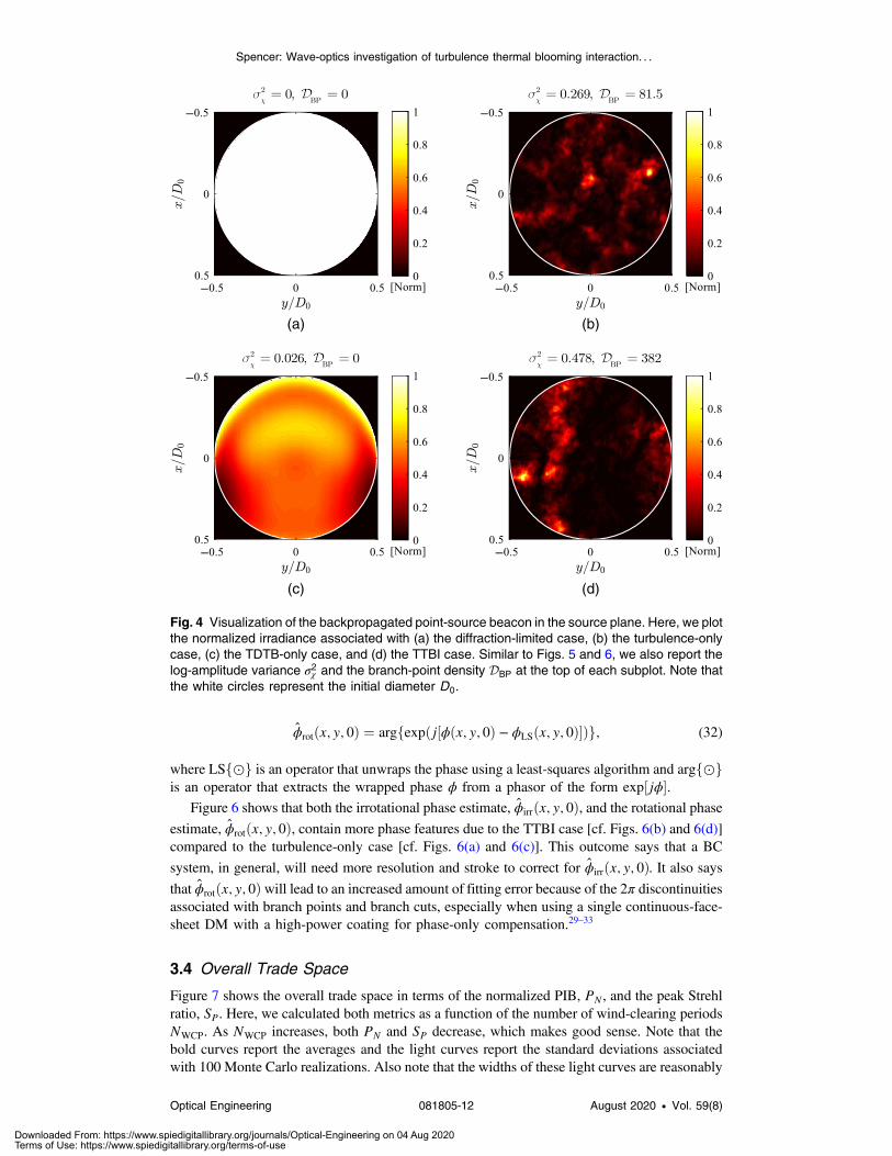
backpropagated point-source beacon due to TTBI. As a result, the log-amplitude variance σ2χ andbranch-point density DBP for the TTBI case would typically increase in comparison to the simu-lated diffraction-limited, turbulence-only, and TDTB-only cases. Figures 4 and 5 demonstratethis hypothesis to be true for one Monte Carlo realization, where Rsw ¼ 0.25, NWCP ¼ 1, andND ¼ NC ¼ 16

ffiffiffi2

p≈ 22.6 [cf. Eqs. (2), (12), and (20), respectively]. Notice that we report val-

ues for both σ2χ and DBP at the top of each normalized irradiance subplot in Fig. 4 and eachwrapped phase subplot in Fig. 5. Also notice that these irradiance subplots are similar but differ-ent to those reported in Part I using steady-state simulations (cf. Figs. 4 and 5 in Part I) since bothpapers use the same Monte Carlo realization of turbulence.

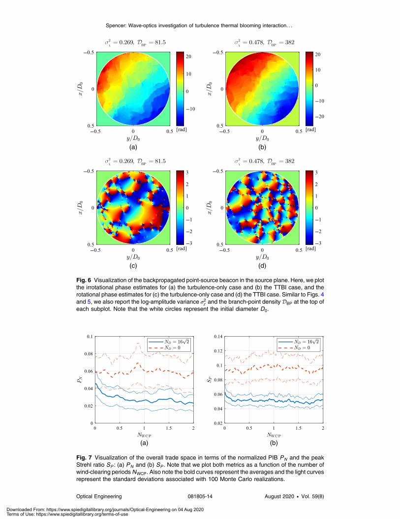
To further explore the effects of TTBI, we also calculated the irrotational phase estimate,

ϕirrðx; y; 0Þ, and rotational phase estimate, ϕrotðx; y; 0Þ. Figure 6 shows these estimates. In prac-tice, these estimates originated from the collimated phase functions ϕðx; y; 0Þ found in Figs. 5(b)and 5(d), for the turbulence-only and TTBI cases, respectively. To calculate ϕirrðx; y; 0Þ and

ϕrotðx; y; 0Þ from ϕðx; y; 0Þ, we used the following relationships:27–31

EQ-TARGET;temp:intralink-;e031;116;106ϕirrðx; y; 0Þ ¼ LSfϕðx; y; 0Þg ¼ ϕLSðx; y; 0Þ (31)

and

(a) (b)

(c) (d)

Fig. 3 Visualization of the focused high-power laser beam in the target plane. Here, we plot thenormalized irradiance associated with (a) the diffraction-limited case, (b) the turbulence-only case,(c) the TDTB-only case, and (d) the TTBI case. We also report the normalized PIB PN and thepeak Strehl ratio SP at the top of each subplot. Note that the white circles represent the diffraction-limited bucket diameter DZ .




EQ-TARGET;temp:intralink-;e032;116;301ϕrotðx; y; 0Þ ¼ argfexpðj½ϕðx; y; 0Þ − ϕLSðx; y; 0Þ�Þg; (32)

where LSf⊙g is an operator that unwraps the phase using a least-squares algorithm and argf⊙gis an operator that extracts the wrapped phase ϕ from a phasor of the form exp½jϕ�.

Figure 6 shows that both the irrotational phase estimate, ϕirrðx; y; 0Þ, and the rotational phaseestimate, ϕrotðx; y; 0Þ, contain more phase features due to the TTBI case [cf. Figs. 6(b) and 6(d)]compared to the turbulence-only case [cf. Figs. 6(a) and 6(c)]. This outcome says that a BC

system, in general, will need more resolution and stroke to correct for ϕirrðx; y; 0Þ. It also says

that ϕrotðx; y; 0Þwill lead to an increased amount of fitting error because of the 2π discontinuitiesassociated with branch points and branch cuts, especially when using a single continuous-face-sheet DM with a high-power coating for phase-only compensation.29–33

3.4 Overall Trade Space

Figure 7 shows the overall trade space in terms of the normalized PIB, PN , and the peak Strehlratio, SP. Here, we calculated both metrics as a function of the number of wind-clearing periodsNWCP. As NWCP increases, both PN and SP decrease, which makes good sense. Note that thebold curves report the averages and the light curves report the standard deviations associatedwith 100 Monte Carlo realizations. Also note that the widths of these light curves are reasonably

(c) (d)

(a) (b)

Fig. 4 Visualization of the backpropagated point-source beacon in the source plane. Here, we plotthe normalized irradiance associated with (a) the diffraction-limited case, (b) the turbulence-onlycase, (c) the TDTB-only case, and (d) the TTBI case. Similar to Figs. 5 and 6, we also report thelog-amplitude variance σ2χ and the branch-point density DBP at the top of each subplot. Note thatthe white circles represent the initial diameter D0.




small, and the bold curves are reasonably smooth. Thus, we will use the same number of MonteCarlo realizations in the analysis that follows.

4 Results and Discussion

This section contains results for the trade space setup in Sec. 2 and explored in Sec. 3. In par-ticular, Fig. 8 shows results for the log-amplitude variance, σ2χ , and the branch-point density,DBP, both as a function of the number of wind-clearing periods NWCP [cf. Eqs. (27), (28), and(12), respectively]. These metrics result from a point-source beacon being backpropagated fromthe target plane to the source plane through the simulated turbulence and TDTB. Here, we useNWCP to help gauge when the time-dependent simulations reach steady state. From Fig. 8, wecan see that both σ2χ and DBP overshoot and settle into steady state when NWCP ≥ 0.5. Thisoutcome is consistent with Fig. 7. Note that in Fig. 8 the bold curves report the averages andthe light curves report the standard deviations associated with 100 Monte Carlo realizations.Also note that the widths of these light curves are reasonably small, and the bold curves arereasonably smooth. Thus, we believe that 100 Monte Carlo realizations (i.e., the same numberof realizations used in Part I of this two-part study) are adequate in quantifying the effectsof TTBI.

(a) (b)

(c) (d)

Fig. 5 Visualization of the backpropagated point-source beacon in the source plane. Here, we plotthe wrapped phase associated with (a) the diffraction-limited case, (b) the turbulence-only case,(c) the TDTB-only case, and (d) the TTBI case. Similar to Figs. 4 and 6, we also report the log-amplitude variance σ2χ and the branch-point density DBP at the top of each subplot. Note that thewhite circles represent the initial diameter D0.




(b)(a)

Fig. 7 Visualization of the overall trade space in terms of the normalized PIB PN and the peakStrehl ratio SP : (a) PN and (b) SP . Note that we plot both metrics as a function of the number ofwind-clearing periodsNWCP. Also note the bold curves represent the averages and the light curvesrepresent the standard deviations associated with 100 Monte Carlo realizations.

(a) (b)

(c) (d)

Fig. 6 Visualization of the backpropagated point-source beacon in the source plane. Here, we plotthe irrotational phase estimates for (a) the turbulence-only case and (b) the TTBI case, and therotational phase estimates for (c) the turbulence-only case and (d) the TTBI case. Similar to Figs. 4and 5, we also report the log-amplitude variance σ2χ and the branch-point density DBP at the top ofeach subplot. Note that the white circles represent the initial diameter D0.




These results clearly show that TTBI results in an increased amount of scintillation whensimulating turbulence and TDTB. For example, as shown in Fig. 8(a), the log-amplitude varianceσ2χ had steady-state averages of 0.437 for the TTBI case (when NWCP ≥ 0.5), and 0.291 for theturbulence-only case (when NWCP ≥ 0). These steady-state averages agreed well with thoseobtained from simulating turbulence and SSTB [cf. the horizontal black lines in Fig. 8(a)], whichhad averages of 0.454 for the TTBI case (whenRsw ¼ 0.25 and ND ¼ NC ¼ 16

ffiffiffi2

p≈ 22.6) and

0.297 for the turbulence-only case (whenRsw ¼ 0.25 and ND ¼ 0), leading to percentage errorsof 3.88% and 1.92%, respectively.

The branch-point densityDBP, as shown in Fig. 8(b), had steady-state averages of 390 for theTTBI case (when NWCP ≥ 0.5), and 127 for the turbulence-only case (when NWCP ≥ 0). Thesesteady-state averages did not agree well with those obtained from simulating turbulence andSSTB [cf. the horizontal black lines in Fig. 8(b)], which had averages of 487 for the TTBI case(whenRsw ¼ 0.25 and ND ¼ NC ¼ 16

ffiffiffi2

p≈ 22.6), and 164 for the turbulence-only case (when

Rsw ¼ 0.25 and ND ¼ 0), leading to percentage errors of 24.8% and 29.3%, respectively. Thislack of agreement was probably due to two phenomena. The first being due to the fact that TTBIdoes not allow the radians of distortion caused by TDTB to equal those caused by SSTB, and thesecond being due to the sensitivity of DBP as a metric.55 Both phenomena warrant further inves-tigation (in subsequent papers). Nonetheless, the results presented in this paper clearly show thatTTBI results in an increased amount of scintillation when simulating turbulence and TDTB.

With the above percentage errors in mind, the time-dependent assumptions contained in thispaper ultimately allowed us to examine the Monte Carlo averages associated with the log-amplitude variance, σ2χ , and the branch-point density,DBP, with increased computational fidelity.However, this increased computational fidelity came at the expense of computational time. Thatis why we reserved the full trade space exploration to Part I of this two-part study. Relative to thetime-dependent results contained in this paper, the steady-state results contained in Part I providean upper bound on both the increase in σ2χ and DBP due to TTBI (cf. Fig. 8 in both papers). It isour hope that such results will prove fruitful in the development of next-generation scaling lawsthat account for the effects of TTBI.39–45

5 Conclusion

In this paper, we used wave-optics simulations to look at the Monte Carlo averages associatedwith turbulence and TDTB. The goal throughout was to investigate TTBI. At a wavelength near

(a) (b)

Fig. 8 Results for the trade space setup in Sec. 2 and explored in Sec. 3: (a) the log-amplitudevariance, σ2χ , and (b) the branch-point density,DBP, both as a function of the number of wind-clear-ing periods NWCP. Here, the bold curves represent the averages and the light curves representthe standard deviations associated with 100 Monte Carlo realizations. It is important to note thatthe black-horizontal lines in (a) and (b) represent the averages (bold lines) and standard deviations(light lines) from simulating 100 Monte Carlo realizations of turbulence and SSTB (cf. Fig. 8 in Part I).




1 μm, TTBI increases the amount of scintillation that results from high-power laser beam propa-gation through distributed-volume atmospheric aberrations. In turn, to help gauge the strength ofthe simulated turbulence and TDTB, this paper made use of the following three parameters: thespherical-wave Rytov number, the number of wind-clearing periods, and the distortion number.These parameters simplified greatly, given a propagation path with constant atmospheric con-ditions. In addition, to help quantify the effects of TTBI, this paper made use of the followingtwo metrics: the log-amplitude variance and branch-point density. These metrics resulted from apoint-source beacon being backpropagated from the target plane to the source plane through thesimulated turbulence and TDTB.

Overall, the results showed that TTBI causes the log-amplitude variance and the branch-pointdensity to increase. These results pose a major problem for BC systems that perform phasecompensation. In turn, the time-dependent simulations presented in this paper will provide muchneeded insight into the design of future systems.

Acknowledgments

The author of this paper would like to thank the Directed Energy Joint Transition Office forsponsoring this research, and C. E. Murphy for many insightful discussions regarding the resultspresented within.

References

1. C. B. Hogge, “Propagation of high-energy laser beams in the atmosphere,” Technical ReportAFWL-TR-74-74, Air Force Weapons Laboratory, Kirtland Air Force Base, New Mexico(1974). http://www.dtic.mil/dtic/tr/fulltext/u2/781763.pdf.

2. D. C. Smith, “High-power laser propagation: thermal blooming,” Proc. IEEE 65(12),1679–1714 (1977).

3. J. L. Ulrich and P. B. Walsh, “Thermal blooming in the atmosphere,” in Laser BeamPropagation in the Atmosphere, J. W. Strohbehn, Ed., Springer-Verlag, Heidelberg,New York (1978).

4. H. Weichel, Laser Beam Propagation in the Atmosphere, SPIE Press, Bellingham,Washington (1989).

5. F. G. Gebhardt, “Twenty-five years of thermal blooming: an overview,” Proc. SPIE 1221,1–25 (1990).

6. N. M. Kroll and P. L. Kelley, “Temporal and spatial gain in stimulated light scattering,”Phys. Rev. A 4(2), 763–776 (1971).

7. T. J. Karr et al., “Perturbation growth by thermal blooming in turbulence,” J. Opt. Soc. Am. A7(6), 1103–1124 (1990).

8. D. H. Chamber et al., “Linear theory of uncompensated thermal blooming in turbulence,”Phys. Rev. A 41(12), 6982–6991 (1990).

9. S. Enguehard and B. Hatfield, “Perturbative approach to the small-scale physics of theinteraction of thermal blooming and turbulence,” J. Opt. Soc. Am A 8(4), 637–646(1991).

10. R. Holmes, R. Myers, and C. Duzy, “A linearized theory of transient laser heating in fluid,”Phys. Rev. A 44(10), 6862–6876 (1991).

11. L. C. Bradley and J. Herrmann, “Phase compensation for thermal blooming,” App. Opt.13(2), 331–334 (1974).

12. J. Herrmann, “Properties of phase conjugate adaptive optical systems,” J. Opt. Soc. Am.67(3), 290–295 (1977).

13. T. J. Karr, “Thermal blooming compensation instabilities,” J. Opt. Soc. Am. A 6(7),1038–1048 (1989).

14. J. R. Morris, “Scalar Green’s-function derivation of the thermal blooming compensationinstability equations,” J. Opt. Soc. Am. A 6(12), 1859–1862 (1989).

15. B. Johnson, “Thermal-blooming laboratory experiments,” Lincoln Lab. J. 5(1), 151–170(1992).




http://www.dtic.mil/dtic/tr/fulltext/u2/781763.pdf




https://doi.org/10.1109/PROC.1977.10809

https://doi.org/10.1117/12.18326

https://doi.org/10.1103/PhysRevA.4.763

https://doi.org/10.1364/JOSAB.7.001103


https://doi.org/10.1364/JOSAA.8.000637


https://doi.org/10.1364/AO.13.000331

https://doi.org/10.1364/JOSA.67.000290



16. J. F. Schonfeld, “Linearized theory of thermal-blooming phase compensation instabilitywith realistic adaptive-optics geometry,” J. Opt. Soc. Am. B 9(10), 1803–1812 (1992).

17. J. R. Morris, J. A. Viecelli, and T. J. Karr, “Effects of a random wind field on thermal bloom-ing instabilities,” Proc. SPIE 1221, 229–240 (1990).

18. J. F. Schonfeld, “The theory of compensated laser propagation through strong thermalblooming,” Lincoln Lab. J. 5(1), 131–150 (1992).

19. D. G. Fouche, C. Higgs, and C. F. Pearson, “Scaled atmospheric blooming experiments,”Lincoln Lab. J. 5(2), 273–293 (1992).

20. D. L. Fried and R. K. Szeto, “Wind-shear induced stabilization of PCI,” J. Opt. Soc. Am. A.15(5), 1212–1226 (1998).

21. J. D. Barchers, “Linear analysis of thermal blooming compensation instabilities in laserpropagation,” J. Opt. Soc. Am. A. 26(7), 1638–1653 (2009).

22. V. P. Lukin and B. V. Fortes, “The influence of wavefront dislocations on phase conjugationinstability with thermal blooming compensation,” Pure Appl. Opt. 6(103) 256–269 (1997).

23. V. P. Lukin and B. V. Fortes, Adaptive Beaming and Imaging in the Turbulent Atmosphere,SPIE Press, Bellingham, Washington (2002).

24. M. F. Spencer et al., “Impact of spatial resolution on thermal blooming phase compensationinstability,” Proc. SPIE 7816, 781609 (2010).

25. M. F. Spencer and S. J. Cusumano, “Impact of branch points in adaptive optics compensa-tion of thermal blooming and turbulence,” Proc. SPIE 8165, 816503 (2011).

26. M. F. Spencer, “Branch point mitigation of thermal blooming phase compensation insta-bility,” MS Thesis, AFIT/OSE/ENP/11-M02, Air Force Institute of Technology, WrightPatterson Air Force Base, Ohio (2011). http://www.dtic.mil/dtic/tr/fulltext/u2/a538538.pdf.

27. D. L. Fried and J. L. Vaughn, “Branch cuts in the phase function,” J. Opt. Soc. Am. A 31(15),2865–2881 (1992).

28. D. L. Fried, “Branch point problem in adaptive optics,” J. Opt. Soc Am. A 15(10),2759–2768 (1998).

29. D. L. Fried, “Adaptive optics wave function reconstruction and phase unwrapping whenbranch points are present,” Opt. Commun. 200, 43–72 (2001).

30. T. M. Venema and J. D. Schmidt, “Optical phase unwrapping in the presence of branchpoints,” Opt. Exp. 16(10), 6985–6998 (2008).

31. M. J. Steinbock, M. W. Hyde, and J. D. Schmidt, “LSPV+7, a branch-point-tolerant recon-structor for strong turbulence adaptive optics,” App. Opt. 53(18), 3821–3831 (2014).

32. M. F. Spencer and T. J. Brennan, “Branch-cut accumulation using LSPV+7,” in Proc. OSApcAOP, p. PTh2D.2 (2017).

33. M. F. Spencer and T. J. Brennan, “Compensation in the presence of deep turbulence usingtiled-aperture architectures,” Proc. SPIE 10194, 1019493 (2017).

34. G. A. Tyler, J. F. Belsher, and P. H. Roberts, “A discussion of some issues associatedwith the evaluation and compensation of thermal blooming,” Technical Report TR-779,The Optical Sciences Company, Anaheim, California (1986).

35. P. H. Roberts, “Time development of thermal blooming,” Technical Report TR-1574,The Optical Sciences Company, Anaheim, California (2002).

36. D. C. Zimmerman, “Wave optics simulation of thermal blooming,” Technical ReportTR-1771, The Optical Sciences Company, Anaheim, California (2008).

37. T. J. Brennan and P. H. Roberts, AOTools the Adaptive Optics Toolbox for Use withMATLAB User’s Guide Version 1.4, The Optical Sciences Company, Anaheim,California (2010).

38. T. J. Brennan, P. H. Roberts, and D. C. Mann, WaveProp a Wave Optics Simulation Systemfor Use with MATLAB User’s Guide Version 1.3, The Optical Sciences Company, Anaheim,California (2010).

39. H. Breaux et al., “Algebraic model for CW thermal-blooming effects,” App. Opt. 18(15),2638–2644 (1979).

40. R. J. Bartell et al., “Methodology for comparing worldwide performance of diverse weight-constrained high energy laser systems,” Proc. SPIE 5792, 76–87 (2005).

41. G. P. Perram et al., Introduction to Laser Weapon Systems, Directed Energy ProfessionalSociety, Albuquerque, New Mexico (2010).




https://doi.org/10.1364/JOSAB.9.001803

https://doi.org/10.1117/12.18345



https://doi.org/10.1088/0963-9659/6/1/012

https://doi.org/10.1117/12.859936

https://doi.org/10.1117/12.894079

http://www.dtic.mil/dtic/tr/fulltext/u2/a538538.pdf




https://doi.org/10.1364/AO.31.002865


https://doi.org/10.1016/S0030-4018(01)01546-2

https://doi.org/10.1364/OE.16.006985

https://doi.org/10.1364/AO.53.003821

https://doi.org/10.1117/12.2258681

https://doi.org/10.1364/AO.18.002638

https://doi.org/10.1117/12.603384

42. N. R. Van Zandt, S. T. Fiorino, and K. J. Keefer, “Enhanced, fast-running scaling law modelof thermal blooming and turbulence effects on high energy laser propagation,” Opt. Exp.21(12), 14789–14798 (2013).

43. S. A. Shakir et al., “General wave optics propagation scaling law,” J. Opt. Soc. Am. A 33(12),2477–2484 (2016).

44. S. A. Shakir et al., “Far-field propagation of partially coherent laser light in random medi-ums,” Opt. Exp. 26(12), 15609–15622 (2018).

45. P. H. Merritt and M. F. Spencer, Beam Control for Laser Systems, 2nd ed., Directed EnergyProfessional Society, Albuquerque, New Mexico (2018).

46. C. E. Murphy and M. F. Spencer, “Investigation of turbulence thermal blooming interactionusing the split-step beam propagation method,” Proc. SPIE 10772, 1077208 (2018).

47. A. Fleck, Jr., J. R. Morris, andM. D. Feit, “Time-dependent propagation of high energy laserbeams through the atmosphere,” Appl. Phys. 10, 129–160 (1976).

48. A. Fleck, Jr., J. R. Morris, andM. D. Feit, “Time-dependent propagation of high energy laserbeams through the atmosphere: II,” Appl. Phys. 14, 99–115 (1977).

49. N. R. Van Zandt et al., “Polychromatic wave-optics models for image-plane speckle. 1.Well-resolved objects,” App. Opt. 57(15), 4090–4102 (2018).

50. N. R. Van Zandt et al., “Polychromatic wave-optics models for image-plane speckle. 2.Unresolved objects,” App. Opt. 57(15), 4103–4110 (2018).

51. J. D. Schmidt, Numerical Simulation of Optical Wave Propagation using MATLAB, SPIEPress, Bellingham, Washington (2010).

52. G. R. Osche, Optical Detection Theory for Laser Applications, John Wiley & Sons,Hoboken, New Jersey (2002).

53. L. C. Andrews and R. L. Phillips, Laser Beam Propagation through Random Media,2nd ed., SPIE Press, Bellingham, Washington (2005).

54. R. J. Sasiela, Electromagnetic Wave Propagation in Turbulence Evaluation and Applicationof Mellin Transforms, 2nd ed., SPIE Press, Bellingham, Washington (2007).

55. J. R. Beck et al., “Investigation of branch-point density using traditional wave-optics tech-niques,” Proc. SPIE 10772, 1077206 (2018).

Mark F. Spencer is a senior research physicist and the principal investigator for Aero Effectsand Beam Control at the Air Force Research Laboratory, Directed Energy Directorate. In addi-tion, he is an adjunct assistant professor of optical sciences and engineering at the Air ForceInstitute of Technology (AFIT), within the Department of Engineering Physics. He receivedhis PhD in optical sciences and engineering from AFIT in 2014. He is a senior member of SPIE.




https://doi.org/10.1364/OE.21.014789


https://doi.org/10.1364/OE.26.015609

https://doi.org/10.1117/12.2319869

https://doi.org/10.1007/BF00896333

https://doi.org/10.1007/BF00882638

https://doi.org/10.1364/AO.57.004090

https://doi.org/10.1364/AO.57.004103

https://doi.org/10.1117/12.2319871

Wave-optics Investigation of Turbulence Thermal Blooming ...

Documents

Transcript of Wave-optics Investigation of Turbulence Thermal Blooming ...