
Water Levels and Long Waves - UTN · EM 1110-2-1100 (Part II) 1 Aug 08 (Change 2) Water Levels and...
76
Water Levels and Long Waves II-5-i Chapter 5 EM 1110-2-1100 WATER LEVELS AND LONG WAVES (Part II) 1 August 2008 (Change 2) Table of Contents Page II-5-1. Introduction ............................................................. II-5-1 a. Purpose ............................................................... II-5-1 b. Applicability ........................................................... II-5-1 c. Scope of manual ........................................................ II-5-1 II-5-2. Classification of Water Waves ............................................ II-5-2 a. Wave classification ...................................................... II-5-2 b. Discussion ............................................................. II-5-5 II-5-3. Astronomical Tides ...................................................... II-5-5 a. Description of tides ...................................................... II-5-5 (1) Introduction ......................................................... II-5-5 (2) Tide-producing forces ................................................. II-5-6 (3) Spring/neap cycle .................................................... II-5-8 (4) Diurnal inequality .................................................... II-5-9 b. Tidal time series analysis ................................................ II-5-11 (1) Introduction ........................................................ II-5-11 (2) Harmonic constituents ............................................... II-5-11 (3) Harmonic reconstruction .............................................. II-5-18 (4) Tidal envelope classification .......................................... II-5-23 c. Glossary of tide elevation terms ........................................... II-5-25 II-5-4. Water Surface Elevation Datums ......................................... II-5-27 a. Introduction ........................................................... II-5-27 b. Tidal-observation-based datums ........................................... II-5-27 c. 1929 NGVD datum ..................................................... II-5-28 d. Great Lakes datums ..................................................... II-5-32 e. Long-term variations in datums ........................................... II-5-32 f. Tidal datums ........................................................... II-5-32 g. Changes in lake level datums ............................................. II-5-37 h. Design considerations ................................................... II-5-38 II-5-5. Storm Surge ............................................................ II-5-38 a. Storm types ........................................................... II-5-38 (1) Tropical storms ..................................................... II-5-39 (2) Extratropical storms ................................................. II-5-42 (3) Surge interaction with tidal elevations ................................... II-5-43 b. Storm event frequency-of-occurrence relationships ............................ II-5-43 (1) Introduction ........................................................ II-5-43 (2) Historical method ................................................... II-5-46 (3) Synthetic method ................................................... II-5-47 (4) Empirical simulation technique ........................................ II-5-47
Transcript of Water Levels and Long Waves - UTN · EM 1110-2-1100 (Part II) 1 Aug 08 (Change 2) Water Levels and...

Water Levels and Long Waves II-5-i
Chapter 5 EM 1110-2-1100WATER LEVELS AND LONG WAVES (Part II)
1 August 2008 (Change 2)
Table of Contents
Page
II-5-1. Introduction . . . . . . . . . . . . . . . . . . . . . . . . . . . . . . . . . . . . . . . . . . . . . . . . . . . . . . . . . . . . . II-5-1a. Purpose . . . . . . . . . . . . . . . . . . . . . . . . . . . . . . . . . . . . . . . . . . . . . . . . . . . . . . . . . . . . . . . II-5-1b. Applicability . . . . . . . . . . . . . . . . . . . . . . . . . . . . . . . . . . . . . . . . . . . . . . . . . . . . . . . . . . . II-5-1c. Scope of manual . . . . . . . . . . . . . . . . . . . . . . . . . . . . . . . . . . . . . . . . . . . . . . . . . . . . . . . . II-5-1
II-5-2. Classification of Water Waves . . . . . . . . . . . . . . . . . . . . . . . . . . . . . . . . . . . . . . . . . . . . II-5-2a. Wave classification . . . . . . . . . . . . . . . . . . . . . . . . . . . . . . . . . . . . . . . . . . . . . . . . . . . . . . II-5-2b. Discussion . . . . . . . . . . . . . . . . . . . . . . . . . . . . . . . . . . . . . . . . . . . . . . . . . . . . . . . . . . . . . II-5-5
II-5-3. Astronomical Tides . . . . . . . . . . . . . . . . . . . . . . . . . . . . . . . . . . . . . . . . . . . . . . . . . . . . . . II-5-5a. Description of tides . . . . . . . . . . . . . . . . . . . . . . . . . . . . . . . . . . . . . . . . . . . . . . . . . . . . . . II-5-5
(1) Introduction . . . . . . . . . . . . . . . . . . . . . . . . . . . . . . . . . . . . . . . . . . . . . . . . . . . . . . . . . II-5-5(2) Tide-producing forces . . . . . . . . . . . . . . . . . . . . . . . . . . . . . . . . . . . . . . . . . . . . . . . . . II-5-6(3) Spring/neap cycle . . . . . . . . . . . . . . . . . . . . . . . . . . . . . . . . . . . . . . . . . . . . . . . . . . . . II-5-8(4) Diurnal inequality . . . . . . . . . . . . . . . . . . . . . . . . . . . . . . . . . . . . . . . . . . . . . . . . . . . . II-5-9
b. Tidal time series analysis . . . . . . . . . . . . . . . . . . . . . . . . . . . . . . . . . . . . . . . . . . . . . . . . II-5-11(1) Introduction . . . . . . . . . . . . . . . . . . . . . . . . . . . . . . . . . . . . . . . . . . . . . . . . . . . . . . . . II-5-11(2) Harmonic constituents . . . . . . . . . . . . . . . . . . . . . . . . . . . . . . . . . . . . . . . . . . . . . . . II-5-11(3) Harmonic reconstruction . . . . . . . . . . . . . . . . . . . . . . . . . . . . . . . . . . . . . . . . . . . . . . II-5-18(4) Tidal envelope classification . . . . . . . . . . . . . . . . . . . . . . . . . . . . . . . . . . . . . . . . . . II-5-23
c. Glossary of tide elevation terms . . . . . . . . . . . . . . . . . . . . . . . . . . . . . . . . . . . . . . . . . . . II-5-25
II-5-4. Water Surface Elevation Datums . . . . . . . . . . . . . . . . . . . . . . . . . . . . . . . . . . . . . . . . . II-5-27a. Introduction . . . . . . . . . . . . . . . . . . . . . . . . . . . . . . . . . . . . . . . . . . . . . . . . . . . . . . . . . . . II-5-27b. Tidal-observation-based datums . . . . . . . . . . . . . . . . . . . . . . . . . . . . . . . . . . . . . . . . . . . II-5-27c. 1929 NGVD datum . . . . . . . . . . . . . . . . . . . . . . . . . . . . . . . . . . . . . . . . . . . . . . . . . . . . . II-5-28d. Great Lakes datums . . . . . . . . . . . . . . . . . . . . . . . . . . . . . . . . . . . . . . . . . . . . . . . . . . . . . II-5-32e. Long-term variations in datums . . . . . . . . . . . . . . . . . . . . . . . . . . . . . . . . . . . . . . . . . . . II-5-32f. Tidal datums . . . . . . . . . . . . . . . . . . . . . . . . . . . . . . . . . . . . . . . . . . . . . . . . . . . . . . . . . . . II-5-32g. Changes in lake level datums . . . . . . . . . . . . . . . . . . . . . . . . . . . . . . . . . . . . . . . . . . . . . II-5-37h. Design considerations . . . . . . . . . . . . . . . . . . . . . . . . . . . . . . . . . . . . . . . . . . . . . . . . . . . II-5-38
II-5-5. Storm Surge . . . . . . . . . . . . . . . . . . . . . . . . . . . . . . . . . . . . . . . . . . . . . . . . . . . . . . . . . . . . II-5-38a. Storm types . . . . . . . . . . . . . . . . . . . . . . . . . . . . . . . . . . . . . . . . . . . . . . . . . . . . . . . . . . . II-5-38
(1) Tropical storms . . . . . . . . . . . . . . . . . . . . . . . . . . . . . . . . . . . . . . . . . . . . . . . . . . . . . II-5-39(2) Extratropical storms . . . . . . . . . . . . . . . . . . . . . . . . . . . . . . . . . . . . . . . . . . . . . . . . . II-5-42(3) Surge interaction with tidal elevations . . . . . . . . . . . . . . . . . . . . . . . . . . . . . . . . . . . II-5-43
b. Storm event frequency-of-occurrence relationships . . . . . . . . . . . . . . . . . . . . . . . . . . . . II-5-43(1) Introduction . . . . . . . . . . . . . . . . . . . . . . . . . . . . . . . . . . . . . . . . . . . . . . . . . . . . . . . . II-5-43(2) Historical method . . . . . . . . . . . . . . . . . . . . . . . . . . . . . . . . . . . . . . . . . . . . . . . . . . . II-5-46(3) Synthetic method . . . . . . . . . . . . . . . . . . . . . . . . . . . . . . . . . . . . . . . . . . . . . . . . . . . II-5-47(4) Empirical simulation technique . . . . . . . . . . . . . . . . . . . . . . . . . . . . . . . . . . . . . . . . II-5-47

EM 1110-2-1100 (Part II)1 Aug 08 (Change 2)
II-5-ii Water Levels and Long Waves
(a) Introduction . . . . . . . . . . . . . . . . . . . . . . . . . . . . . . . . . . . . . . . . . . . . . . . . . . . . . . . . II-5-47(b) EST - tropical storm application . . . . . . . . . . . . . . . . . . . . . . . . . . . . . . . . . . . . . . . . II-5-47(c) EST - extratropical storm application . . . . . . . . . . . . . . . . . . . . . . . . . . . . . . . . . . . . II-5-49
II-5-6. Seiches . . . . . . . . . . . . . . . . . . . . . . . . . . . . . . . . . . . . . . . . . . . . . . . . . . . . . . . . . . . . . . . . II-5-51
II-5-7. Numerical Modeling of Long-Wave Hydrodynamics . . . . . . . . . . . . . . . . . . . . . . . . II-5-54a. Long-wave modeling . . . . . . . . . . . . . . . . . . . . . . . . . . . . . . . . . . . . . . . . . . . . . . . . . . . . II-5-54b. Physical models . . . . . . . . . . . . . . . . . . . . . . . . . . . . . . . . . . . . . . . . . . . . . . . . . . . . . . . . II-5-54c. Numerical models . . . . . . . . . . . . . . . . . . . . . . . . . . . . . . . . . . . . . . . . . . . . . . . . . . . . . . II-5-55
(1) Introduction . . . . . . . . . . . . . . . . . . . . . . . . . . . . . . . . . . . . . . . . . . . . . . . . . . . . . . . . II-5-55(2) Example - tidal circulation modeling . . . . . . . . . . . . . . . . . . . . . . . . . . . . . . . . . . . . II-5-56(3) Example - storm surge modeling . . . . . . . . . . . . . . . . . . . . . . . . . . . . . . . . . . . . . . . II-5-57
II-5-8. References . . . . . . . . . . . . . . . . . . . . . . . . . . . . . . . . . . . . . . . . . . . . . . . . . . . . . . . . . . . . . II-5-64
II-5-9. Definitions of Symbols . . . . . . . . . . . . . . . . . . . . . . . . . . . . . . . . . . . . . . . . . . . . . . . . . . II-5-69
II-5-10. Acknowledgments . . . . . . . . . . . . . . . . . . . . . . . . . . . . . . . . . . . . . . . . . . . . . . . . . . . . . II-5-71

EM 1110-2-1100 (Part II)1 Aug 08 (Change 2)
Water Levels and Long Waves II-5-iii
List of Tables
Page
Table II-5-1. Wave Classification (Ippen 1966) . . . . . . . . . . . . . . . . . . . . . . . . . . . . . . . . . . . . . . II-5-3
Table II-5-2. Hyperbolic Function Asymptotes . . . . . . . . . . . . . . . . . . . . . . . . . . . . . . . . . . . . . . . II-5-4
Table II-5-3. NOS Tidal Constituents and Arguments . . . . . . . . . . . . . . . . . . . . . . . . . . . . . . . . II-5-16
Table II-5-4. Node Factors for 1970 through 1999 (Schureman 1924) . . . . . . . . . . . . . . . . . . . . II-5-17
Table II-5-5. Equilibrium Argument for Beginning of Years 2001 through 2010 (Schureman 1924) . . . . . . . . . . . . . . . . . . . . . . . . . . . . . . . . . . . . . . . . . . . . . . . . . II-5-19
Table II-5-6. Summary of Harmonic Arguments for Sandy Hook, NJ (1 January 1984 at 0000 hr) . . . . . . . . . . . . . . . . . . . . . . . . . . . . . . . . . . . . . . . . . . . . . . . . . . . . . . . II-5-23
Table II-5-7. Datums for Reference Tide Stations (Harris 1981) . . . . . . . . . . . . . . . . . . . . . . . . II-5-29
Table II-5-8. Low Water (chart) Datum for IGLD 1955 and IGLD 1985 . . . . . . . . . . . . . . . . . . II-5-35

EM 1110-2-1100 (Part II)1 Aug 08 (Change 2)
II-5-iv Water Levels and Long Waves
List of Figures
Page
Figure II-5-1. Long wave geometry (Milne-Thompson 1960) . . . . . . . . . . . . . . . . . . . . . . . . . . . . II-5-3
Figure II-5-2. Variation of particle velocity with depth (Ippen 1966) . . . . . . . . . . . . . . . . . . . . . . II-5-4
Figure II-5-3. Schematic representation of water particle trajectories (Ippen 1966) . . . . . . . . . . . II-5-5
Figure II-5-4. Schematic diagram of tidal potential (Dronkers 1964) . . . . . . . . . . . . . . . . . . . . . . II-5-7
Figure II-5-5. Tide predictions for Boston, MA (Harris 1981) . . . . . . . . . . . . . . . . . . . . . . . . . . . . II-5-9
Figure II-5-6. Spring and neap tides (Shalowitz 1964) . . . . . . . . . . . . . . . . . . . . . . . . . . . . . . . . . II-5-10
Figure II-5-7. The daily inequality (Dronkers 1964) . . . . . . . . . . . . . . . . . . . . . . . . . . . . . . . . . . II-5-11
Figure II-5-8. Typical tide curves along the Atlantic and Gulf coasts (Shore Protection Manual 1984) . . . . . . . . . . . . . . . . . . . . . . . . . . . . . . . . . . . . . . . . . . . . . . . . . . . . . II-5-12
Figure II-5-9. Typical tide curves along Pacific coasts of the United States (Shore Protection Manual 1984) . . . . . . . . . . . . . . . . . . . . . . . . . . . . . . . . . . . . . . . . . . . . . . . . . . . . . II-5-13
Figure II-5-10. Tidal phase relationships . . . . . . . . . . . . . . . . . . . . . . . . . . . . . . . . . . . . . . . . . . . . II-5-18
Figure II-5-11. Phase angle argument relationship . . . . . . . . . . . . . . . . . . . . . . . . . . . . . . . . . . . . . II-5-20
Figure II-5-12. NOS harmonic analysis for Sandy Hook, NJ . . . . . . . . . . . . . . . . . . . . . . . . . . . . . II-5-21
Figure II-5-13. Tide tables for Sandy Hook, NJ (NOAA 1984) . . . . . . . . . . . . . . . . . . . . . . . . . . . II-5-22
Figure II-5-14. Reconstructed tidal envelope for Sandy Hook, NJ . . . . . . . . . . . . . . . . . . . . . . . . . II-5-24
Figure II-5-15. Areal extent of tidal types (Harris 1981) . . . . . . . . . . . . . . . . . . . . . . . . . . . . . . . . II-5-25
Figure II-5-16. Types of tides (Shore Protection Manual 1984) . . . . . . . . . . . . . . . . . . . . . . . . . . II-5-26
Figure II-5-17. Reference and comparative tide stations, Atlantic, Gulf, and Pacific coasts (Harris 1981) . . . . . . . . . . . . . . . . . . . . . . . . . . . . . . . . . . . . . . . . . . II-5-31
Figure II-5-18. Locations of tide stations used in establishing the National Geodetic Vertical Datum (NGVD) of 1929 (Harris 1981 (after Rappleye (1932)) . . . . . . . . II-5-33
Figure II-5-19. Sample NOS description of tidal bench marks (Harris 1981) . . . . . . . . . . . . . . . . II-5-34
Figure II-5-20. Vertical and horizontal relationships for the IGLD 1985 . . . . . . . . . . . . . . . . . . . . II-5-35
Figure II-5-21. Sample NOS tabulation of tide parameters (Harris 1981) . . . . . . . . . . . . . . . . . . . II-5-39
EM 1110-2-1100 (Part II)1 Aug 08 (Change 2)
Water Levels and Long Waves II-5-v
Figure II-5-22. Variations in annual MSL (Harris 1981) . . . . . . . . . . . . . . . . . . . . . . . . . . . . . . . . II-5-40
Figure II-5-23. Schematic diagram of storm parameters (U.S. Army Corps of Engineers 1986) . . . . . . . . . . . . . . . . . . . . . . . . . . . . . . . . . . . . . . . . . . . . . . . . . II-5-41
Figure II-5-24. Hurricane Gloria track from 17 September to 2 October 1985 (Jarvinen and Gebert 1986) . . . . . . . . . . . . . . . . . . . . . . . . . . . . . . . . . . . . . . . . . . . . . . . . . . II-5-44
Figure II-5-25. Hurricane Gloria track offshore of Delaware and New Jersey (Jarvinen and Gebert 1986) . . . . . . . . . . . . . . . . . . . . . . . . . . . . . . . . . . . . . . . . . . . . . . . . . . II-5-45
Figure II-5-26. Example phasing of storm surge and tide (Jarvinen and Gebert 1986) . . . . . . . . . II-5-46
Figure II-5-27. Stage-frequency relationship - coast of Delaware . . . . . . . . . . . . . . . . . . . . . . . . . II-5-50
Figure II-5-28. Sediment transport magnitude-frequency relationship - December 1992 Northeaster . . . . . . . . . . . . . . . . . . . . . . . . . . . . . . . . . . . . . . . . . . . . . . . . . . . . . . . II-5-51
Figure II-5-29. Atlantic tropical storm tracks during the period 1886-1980 . . . . . . . . . . . . . . . . . II-5-52
Figure II-5-30. Long wave surface profiles (Shore Protection Manual 1984) . . . . . . . . . . . . . . . . II-5-53
Figure II-5-31. First, second, and third normal modes of oscillation for Lake Ontario (Rao and Schwab 1976) . . . . . . . . . . . . . . . . . . . . . . . . . . . . . . . . . . . . . . . . . . . . . II-5-54
Figure II-5-32. Computational grid for the New York Bight . . . . . . . . . . . . . . . . . . . . . . . . . . . . . II-5-58
Figure II-5-33. Model and prototype tidal elevation comparison at the Battery . . . . . . . . . . . . . . . II-5-59
Figure II-5-34. Wind-induced circulation pattern . . . . . . . . . . . . . . . . . . . . . . . . . . . . . . . . . . . . . . II-5-60
Figure II-5-35. Global limits of ADCIRC computational grid . . . . . . . . . . . . . . . . . . . . . . . . . . . . II-5-61
Figure II-5-36. Blow-up of ADCIRC grid along Delaware coast . . . . . . . . . . . . . . . . . . . . . . . . . . II-5-62
Figure II-5-37. Model-to-prototype tidal comparison at Lewes, DE . . . . . . . . . . . . . . . . . . . . . . . II-5-63
Figure II-5-38. Model-to-prototype surge comparison at Lewes, DE . . . . . . . . . . . . . . . . . . . . . . . II-5-64

EM 1110-2-1100 (Part II)1 Aug 08 (Change 2)
Water Levels and Long Waves II-5-1
Chapter II-5Water Levels and Long Waves
II-5-1. Introduction
a. Purpose.
(1) This chapter describes water levels and the various long wave components that contribute to a totalwater surface elevation. Vertical datums are also described to define some of the more commonly usedreference datums.
(2) The following sections provide project engineers with sufficient guidance to develop a preliminarystudy approach and design procedure to analyze engineering projects that require consideration of water levelelevations. References are provided from existing Engineer Manuals that describe generic design-criteriaformulae for use in preliminary analyses. Additional references and approaches to problem solving areprovided for complex projects that require detailed surface elevation and current input data for design. Thesedata are generally provided by numerical models.
b. Applicability. Information contained in this chapter is directly applicable to any project requiringlocal water levels or currents as a primary design consideration. Applications include the design of coastalstructures intended to provide protection against some pre-defined water surface elevation, specifiedaccording to an appropriate economic analysis and evaluation. Determining acceptable design elevations mayrequire developing local stage relationships as opposed to frequency-of-occurrence relationships. Thisinformation can be generated through historical records or numerical modeling techniques to simulate thepropagation of historical storm events. Additional examples of water surface and current variability includecircumstances where tidal circulation patterns and surface elevations change as a result of structural orbathymetric modifications to existing coastal inlets or navigable waterways. These circulation-dominatedproblems can be addressed using either numerical or physical models.
c. Scope of manual.
(1) Water wave classification is used to describe the behavior of long waves and to distinguish betweenintermediate waves and short waves (described in Part II-2). This allows the reader to select which chapterof this manual is appropriate for the intended application. If long waves are appropriate, this chapter willprovide a means of approximating basic wave characteristics such as celerity, current magnitudes, and surfaceelevation.
(2) The speed of propagation, surface profile, and vertical velocity distribution of long waves aredifferent from those of short waves described in Part II-2. Because these properties of waves representimportant design criteria, it is important to make a distinction between long and short waves. Therefore,Part II-5-2 reviews wave classification criteria and summarizes long wave properties.
(3) Tides are the most common and visible example of long wave propagation. Part II-5-3 summarizestidal hydrodynamics and describes characteristic tidally induced long wave variability. This section includesa background description of the forces responsible for generating tides, gives examples of the variability oftides, and presents a methodology for harmonic reconstruction of tides.
(4) Many of the concepts described by tidal records are used as a basis for defining tidal datums.Part II-5-4 describes reference elevation datums commonly in use in the United States. Attention is also paid

EM 1110-2-1100 (Part II)1 Aug 08 (Change 2)
II-5-2 Water Levels and Long Waves
to the change in coastal datums that may result from sea (or lake) level rise and/or land subsidence orrebound.
(5) Parts II-5-5 through II-5-7 describe nontidal variability in water surfaces. These fluctuations can bestorm-generated, as in the case of tropical and extratropical storms; atmospheric- and geometry-related, asin the case of seiches or tidal bores; or be due to responses stemming from earthquake-generated tsunamisor other rapid changes in the environment.
(6) The primary goal of this chapter is to define tidal and storm-generated fluctuations in the watersurface and describe the datums to which they are referenced. Seiches will only be briefly discussed andtsunamis are not addressed because a special report on tsumanis has been prepared by the Coastal andHydraulics Laboratory (CHL) (Camfield 1980). In addition to Camfield, Engineer Manual 1110-2-1414,“Water Levels and Wave Heights for Coastal Engineering Design,” addresses the propagation of tsunamis.However, because both seiches and tsunamis are classified as long waves, the numerical modeling techniquesdiscussed in Part II-5-7 are an appropriate means of analysis.
II-5-2. Classification of Water Waves
a. Wave classification.
(1) The long wave descriptions that follow are based on small-amplitude wave theory solutions to thegoverning equations. This theory places certain criteria on the physical shape of the wave. For example,from Figure II-5-1, the amplitude is assumed small with respect to the depth (i.e., 0/h ratio is small, and thesurface slope d0/dx is assumed small).
(2) Although wave amplitude is assumed small with respect to depth, the manner in which the wavepropagates is a function of just how small this ratio is. The propagation of small-amplitude waves in watercan now be described as a function of the wave length and the depth of water in which the wave ispropagating. In fact, waves can be classified according to a parameter referred to as the “relative depth,”defined as the ratio of water depth h to wave length L. When this ratio is less than approximately 1/20, wavescan be classified as long waves or “shallow-water waves.” Figure II-5-1 shows typical long wave geometryfor a wave whose length L is large with respect to the depth of water h.
(3) Astronomical tides represent one important example of long waves. In Chesapeake Bay, for example,the M2 primary lunar tidal constituent is contained completely within the Bay at a given instant in time,producing a wavelength of approximately 300 km. The mean depth of flow in the Bay is approximately 10m; therefore, the relative depth is 3.3 × 10⁻⁵. Long waves are not limited to what is normally consideredshallow water because the relative depth is a function of wavelength. In fact, most tides are long waves overthe entire ocean because their wavelengths are on the order of 1,000 km and depths are on the order ofkilometers. Similarly, seismic-forced phenomena such as tsunamis propagate across the Pacific Ocean indepths of up to 20 km but have wavelengths on the order of hundreds of kilometers.
(4) Waves are classified as short waves, also referred to as “deepwater waves,” when the relative depthis greater than approximately 1/2. Coastal waves described in Part II-2 are generally of this class. Thegeometry of short waves implies wave steepness great enough to cause them to break. The class of wavesbetween short (deep) and long (shallow) are referred to as “intermediate waves.” Table II-5-1 (Ippen

EM 1110-2-1100 (Part II)1 Aug 08 (Change 2)
Water Levels and Long Waves II-5-3
Figure II-5-1. Long wave geometry (Milne-Thompson 1960)
Table II-5-1Wave Classification (Ippen 1966)
Range of h/L Range of kh=2Bh/L Types of waves
0 to 1/20 0 to B/10 Long waves (shallow-water wave)
1/20 to 1/2 B/10 to B Intermediate waves
1/2 to 4 B to 4 Short waves (deepwater waves)
1966) summarizes wave classification criteria according to relative depth and the wave parameter kh definedbelow.
(5) Applying the relative depth and wave number parameter to the characteristics of long waves can beseen in the simplification to progressive small-amplitude wave theory solutions. For example, from Part II-1,the wave celerity, wave length, horizontal (x-direction) and vertical velocities can be written as
(II-5-1)
(II-5-2)
(II-5-3)
(II-5-4)
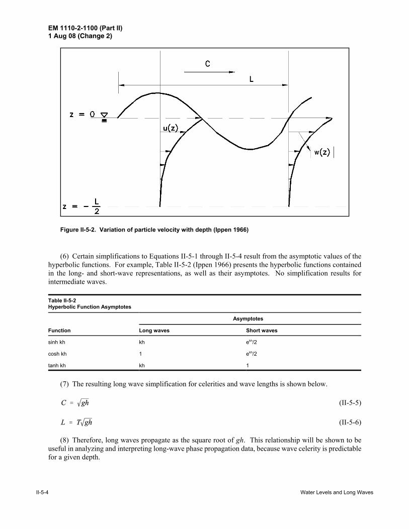
where k is the wave number (2B/L), F is the angular frequency (2B/T where T is the period of the wave), ais the amplitude of the wave, g the acceleration of gravity, h is the total depth, and z is the depth measureddownward from the quiescent fluid surface. A schematic diagram of the variation of velocity as a functionof depth is shown in Figure II-5-2.
EM 1110-2-1100 (Part II)1 Aug 08 (Change 2)
II-5-4 Water Levels and Long Waves
Figure II-5-2. Variation of particle velocity with depth (Ippen 1966)
(6) Certain simplifications to Equations II-5-1 through II-5-4 result from the asymptotic values of thehyperbolic functions. For example, Table II-5-2 (Ippen 1966) presents the hyperbolic functions containedin the long- and short-wave representations, as well as their asymptotes. No simplification results forintermediate waves.
Table II-5-2Hyperbolic Function Asymptotes
Function
Asymptotes
Long waves Short waves
sinh kh kh ekh/2
cosh kh 1 ekh/2
tanh kh kh 1
(7) The resulting long wave simplification for celerities and wave lengths is shown below.
(II-5-5)
(II-5-6)
(8) Therefore, long waves propagate as the square root of gh. This relationship will be shown to beuseful in analyzing and interpreting long-wave phase propagation data, because wave celerity is predictablefor a given depth.
EM 1110-2-1100 (Part II)1 Aug 08 (Change 2)
Water Levels and Long Waves II-5-5
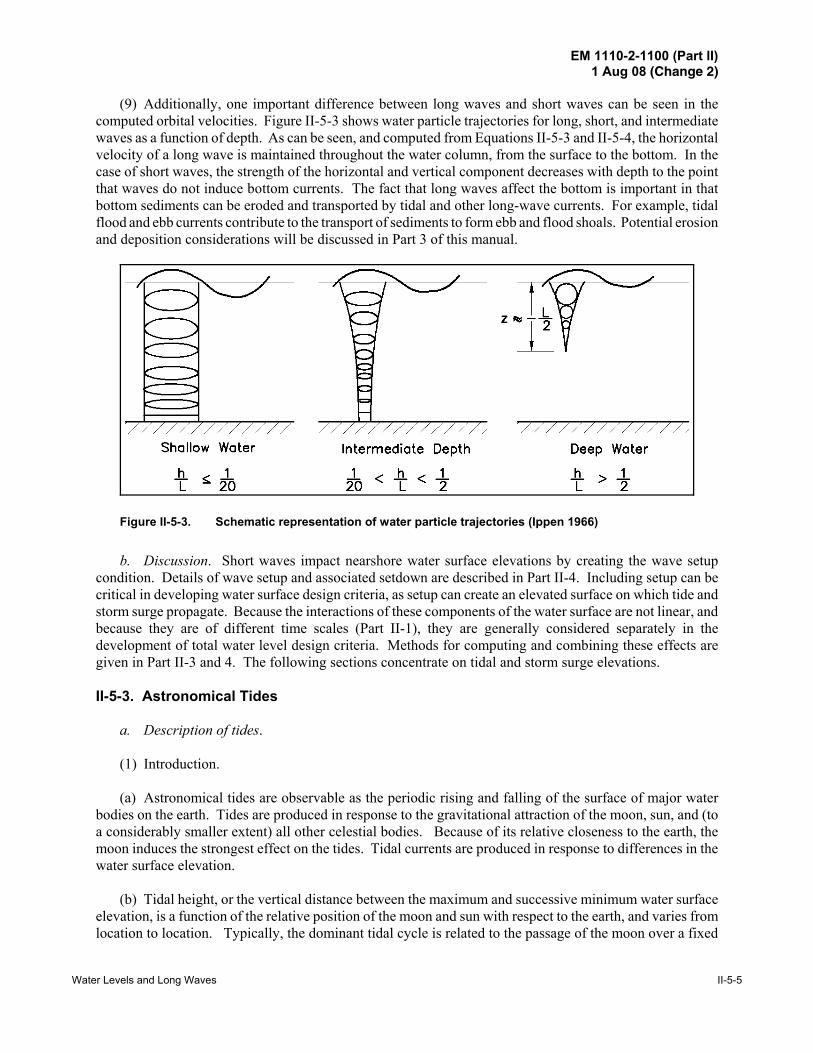
Figure II-5-3. Schematic representation of water particle trajectories (Ippen 1966)
(9) Additionally, one important difference between long waves and short waves can be seen in thecomputed orbital velocities. Figure II-5-3 shows water particle trajectories for long, short, and intermediatewaves as a function of depth. As can be seen, and computed from Equations II-5-3 and II-5-4, the horizontalvelocity of a long wave is maintained throughout the water column, from the surface to the bottom. In thecase of short waves, the strength of the horizontal and vertical component decreases with depth to the pointthat waves do not induce bottom currents. The fact that long waves affect the bottom is important in thatbottom sediments can be eroded and transported by tidal and other long-wave currents. For example, tidalflood and ebb currents contribute to the transport of sediments to form ebb and flood shoals. Potential erosionand deposition considerations will be discussed in Part 3 of this manual.
b. Discussion. Short waves impact nearshore water surface elevations by creating the wave setupcondition. Details of wave setup and associated setdown are described in Part II-4. Including setup can becritical in developing water surface design criteria, as setup can create an elevated surface on which tide andstorm surge propagate. Because the interactions of these components of the water surface are not linear, andbecause they are of different time scales (Part II-1), they are generally considered separately in thedevelopment of total water level design criteria. Methods for computing and combining these effects aregiven in Part II-3 and 4. The following sections concentrate on tidal and storm surge elevations.
II-5-3. Astronomical Tides
a. Description of tides.
(1) Introduction.
(a) Astronomical tides are observable as the periodic rising and falling of the surface of major waterbodies on the earth. Tides are produced in response to the gravitational attraction of the moon, sun, and (toa considerably smaller extent) all other celestial bodies. Because of its relative closeness to the earth, themoon induces the strongest effect on the tides. Tidal currents are produced in response to differences in thewater surface elevation.
(b) Tidal height, or the vertical distance between the maximum and successive minimum water surfaceelevation, is a function of the relative position of the moon and sun with respect to the earth, and varies fromlocation to location. Typically, the dominant tidal cycle is related to the passage of the moon over a fixed

EM 1110-2-1100 (Part II)1 Aug 08 (Change 2)
II-5-6 Water Levels and Long Waves
meridian. This occurs an average of 50 min later each succeeding day. This passage of the moon producesapproximately two tides per solar day (referred to as semidiurnal), with a maximum tide occurringapproximately every 12 hr 25 min. However, differences in the relationship of the moon and sun inconjunction with local conditions can result in tides that exhibit only one tidal cycle per day. These arereferred to as diurnal tides. Mixed tides exhibit characteristics of both semidiurnal and diurnal tides. Atcertain times in the lunar month, two peaks per day are produced, while at other times the tide is diurnal. Thedistinction is explained in the following paragraphs.
(c) The description of typical tidal variability begins with a brief background description of tide-producing forces, those gravitational forces responsible for tidal motion, and the descriptive tidal envelopethat results from those forces. This sub-section will be followed by more qualitative descriptions of how thetidal envelope is influenced by the position of the moon and sun. Once this basic pattern is established,measured tidal elevations can, in part, be shown to be a function of the influence of the continental shelf andthe coastal boundary on the propagating tide.
(2) Tide-producing forces.
(a) The law of universal gravitation was first published by Newton in 1686. Newton's law of gravitationstates that every particle of matter in the universe attracts every other particle with a force that is directlyproportional to the product of the masses of the particles and inversely proportional to the square of thedistance between them (Sears and Zemansky 1963). Quantitative aspects of the law of gravitational attractionbetween two bodies of mass m1 and m2 can be written as follows:
(II-5-7)
where Fg is the gravitational force on either particle, r is separation of distance between the centers of massof the two bodies, and f is the universal constant with a value of 6.67 × 10⁻⁸ cm3/gm sec2. The gravitationalforce of the earth on particle m1 can be determined from Equation II-5-7. Let Fg = m1 g where g is theacceleration of gravity (980.6 cm/sec2) on the surface of the earth, and m2 equal the mass of the earth E. Bysubstitution, an expression for the gravitational constant can be written in terms of the radius of the earth aand the acceleration of gravity g.
(II-5-8)
(b) Development of the tidal potential follows directly from the above relationship. The followingvariables are referenced to Figure II-5-4 (although Figure II-5-4 refers to the moon, an analogous figure canbe drawn for the sun). Let M and S be the mass of the moon and sun, respectively. rm and rs are the distancesfrom the center of the earth O to the center of the moon and sun. Let rmx and rsx be the distances of a pointX(x,y,z) located on the surface of the earth to the center of the moon and sun. The following relationshipsdefine the tidal potential at some arbitrary point X as a function of the relative position of the moon and sun.
(c) The attractive force potentials per unit mass for the moon and sun can be written as
(II-5-9)

EM 1110-2-1100 (Part II)1 Aug 08 (Change 2)
Water Levels and Long Waves II-5-7
Figure II-5-4. Schematic diagram of tidal potential (Dronkers 1964)
where the separation distance rMX = [(xm - x)2 + (ym - y)2 + (zm - z)2]1/2 with an equivalent expression for rSX.
(d) The attractive force of the moon and sun at any point X is defined as
(II-5-10)
where L is the vector gradient operator defined as
(II-5-11)
(e) From Figure II-5-4, the attractive force at the center of the earth (centripetal) bO is balanced by thecentrifugal force -bO (i.e., equal in magnitude but opposite in direction). Because any point on the earthexperiences the same centrifugal force as that at O, the resultant force at any point X will be equal to bX - bO.This resultant force difference is the tide generating force, the force that causes the oceans to deform in orderto balance the sum of external forces. Therefore, the difference between the tidal potential at point O and atpoint X becomes the tidal potential responsible for the tide-producing forces.
(f) The moon’s tide-generating potential can be written as
(II-5-12)
with the tide potential for the sun written as

EM 1110-2-1100 (Part II)1 Aug 08 (Change 2)
II-5-8 Water Levels and Long Waves
(II-5-13)
where a is the mean radius of the earth. Various geometric relationships are used to write Equations II-5-12and II-5-13 in the following forms:
(II-5-14)
(II-5-15)
where the terms PM and PS represent harmonic polynomial expansion terms that collectively describe therelative positions of the earth, moon, and sun. Note that in both cases, the tidal potential term is written asan inverse function of the distance between the earth and the moon or sun. Both Dronkers (1964) andSchureman (1924) present detailed derivations of the terms of Equations II-5-14 and II-5-15. For the purposeof this manual, however, the tidal potential terms shown here are adequate to describe the two most importantfeatures of a tidal record, the spring/neap cycle and the diurnal inequality.
(3) Spring/neap cycle.
(a) The semidiurnal rise and fall of tide can be described as nearly sinusoidal in shape, reaching a peakvalue every 12 hr and 25 min. This period represents one-half of the lunar day. Two tides are generallyexperienced per lunar day because tides represent a response to the increased gravitational attraction fromthe (primarily) moon on one side of the earth, balanced by a centrifugal force on the opposite side of the earth.These forces create a “bulge” or outward deflection in the water surface on the two opposing sides of theearth.
(b) The magnitude of tidal deflection is partially a function of the distance between the moon and earth.When the moon is in perigee, i.e., closest to the earth, the tide range is greater than when it is furthest fromthe earth, in apogee. For example, the potential terms in Equation II-5-14 contain the multiplier 1/rM,describing the distance of the moon from the earth. When the moon is closest to the earth, rM is a minimumvalue and the tidal potential term is maximum. Conversely, when the moon is in apogee, the potential termis at a minimum value. This difference may be as large as 20 percent.
(c) The maximum water surface deflection of semidiurnal tides changes as the relative position of themoon and sun changes. The amplitude envelope connecting any two successive high tides (and low tides)gradually increases from some minimum height to a maximum value, and then decreases back to a minimum.Periods of maximum amplitude are referred to as spring tides, times of minimum amplitude are neap tides.This envelope of spring to neap occurs twice over a period of approximately 29 days. An example tidal signalfor Boston, MA, is shown in Figure II-5-5 (Harris 1981) in which the normalized tidal signal exhibits twoamplitude envelopes during the total time series.
(d) Spring tides occur when the sun and moon are in alignment. This occurs at either a new moon, whenthe sun and moon are on the same side of the earth, or at full moon, when they are on opposite sides of theearth. Neap tides occur at the intermediate points, the moon's first and third quarters. Figure II-5-6 is aschematic representation of these predominant tidal phases. Lunar quarters are indicated in the tidal time

EM 1110-2-1100 (Part II)1 Aug 08 (Change 2)
Water Levels and Long Waves II-5-9
Figure II-5-5. Tide predictions for Boston, MA (Harris 1981)
series shown in Figure II-5-5. Note that in Figure II-5-5, the envelope that connects higher-high tide valuesfor the first spring tide during the first 14.5 days becomes an envelope of the lower-high tide values duringthe second spring tide.
(4) Diurnal inequality.
(a) In the above example, the envelope of two successive high or low tides defines spring and neapconditions. Alternate tides were used because the ranges of two successive tides at a given location aregenerally not identical, but exhibit differences in height. Examples are evident in Figure II-5-5. Thesedifferences are referred to as the diurnal inequality of the tide and result from the relative position of the sunand moon as well as the specific location of an observer on the earth.

EM 1110-2-1100 (Part II)1 Aug 08 (Change 2)
II-5-10 Water Levels and Long Waves
Figure II-5-6. Spring and neap tides (Shalowitz 1964)
(b) Diurnal inequality can be explained as follows. The tidal bulge is centered along a line from thecenter of the moon or sun to the center of the earth. The tidal bulge at a given sublunar or subsolar (locationon the earth nearest the moon or sun) location has an equivalent bulge on the opposite side of the earth, i.e.,on a line drawn from the sublunar or subsolar point through the center of the earth on the opposite side of theequator. If the sublunar or subsolar point appears at a given north latitude, the peak of the corresponding tidalbulge on the opposite side of the equator will appear at a corresponding south latitude. Thus, a point on thesame north latitude but 180 deg in longitude from the sublunar or subsolar point will show a reducedamplitude.
(c) A schematic example of the daily inequality is presented by Dronkers (1964) for the simple case ofan earth-moon system. Referring to Figure II-5-7, the moon is located in the direction M and earth is rotatingabout the polar axis P. The deformed water surface resulting in response to the tide-producing forces isshown in the figure. Four locations (I - IV) are indicated to demonstrate the effect of location on the diurnalinequality. The fluctuating tide can be seen as the deviation in the deformed surface from a line at constantlatitude on the undeformed spherical surface corresponding to each location. Location I corresponds to anobserver on the equator. In this case, it can be seen that the tidal deformations from static conditions areequal; therefore, there is no diurnal inequality, each high tide is equal. However, at locations II and III, theinequality is evident with the second tide being substantially lower than the first. In the extreme case,location IV exhibits a diurnal tide only due to its location with respect to the deformed water surface.
(d) The combinations of astronomical forcing that define spring and neap cycles and diurnal inequalitiesis further modified by local bathymetry and shoreline boundary influences. All of these factors combine toproduce tidal envelopes that vary from location to location. The result is site-specific tidal signatures, whichcan be classified as semidiurnal, diurnal, or mixed. Examples of these classes of tides are shown inFigures II-5-8 and II-5-9. Tides along the Atlantic coast are generally semidiurnal with a small diurnalinequality. Typical east coast envelopes for Boston, MA; New York, NY; Hampton Roads, (Hampton), VA;

EM 1110-2-1100 (Part II)1 Aug 08 (Change 2)
Water Levels and Long Waves II-5-11
Figure II-5-7. The daily inequality (Dronkers 1964)
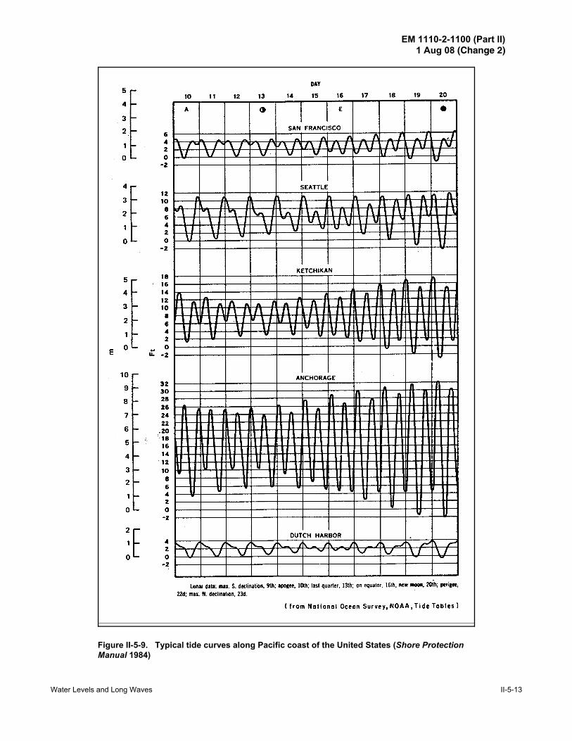
and the entrance to the Savannah River at Savannah, GA, are shown in the figure. Each time series exhibitstwo distinct and nearly equal tides per day. As one moves to Key West, FL, the character of the tide beginsto change with a noticeable diurnal inequality. Tides inside the Gulf of Mexico range from semidiurnal atKey West, FL, to diurnal at Pensacola, FL, to mixed at Galveston, TX. Note that the Galveston dataprogresses from a diurnal tide during the first third of the record to a semidiurnal tide. Tides in the Gulf ofMexico are more complex than open ocean stations because astronomical forcing is modified bygeometrically forced nodes and antinodes. These seiche-related phenomena are discussed in Part II-5-6.Pacific coast tides, shown in Figure II-5-9, are generally of larger amplitude than Atlantic and Gulf coast tidesand often have a decided diurnal inequality.
b. Tidal time series analysis.
(1) Introduction. The equilibrium theory of tides is a hypothesis that the waters of the earth respondinstantaneously to the tide-producing forces of the sun and moon. For example, high water occurs directlybeneath the moon and sun, i.e., at the sublunar and subsolar points. This tide is referred to as an equilibriumtide. Part II-5-3 a (1), states that tide-producing forces are written in a polynomial expansion approximationfor the exact solution of Equations II-5-12 and II-5-13. These expansion terms involve astronomicalarguments describing the location of the sun and moon as well as the location of the observer on the earth.Although several variational forms of the series expansion have been published, the development presentedin Schureman (1924) is given below. Alternate forms of expansion are discussed in Dronkers (1964).
(2) Harmonic constituents.
(a) According to equilibrium theory, the theoretical tide can be predicted at any location on the earth asa sum of a number of harmonic terms contained in the polynomial expansion representation of the

EM 1110-2-1100 (Part II)1 Aug 08 (Change 2)
II-5-12 Water Levels and Long Waves
Figure II-5-8. Typical tide curves along the Atlantic and Gulf coasts (Shore ProtectionManual 1984)
EM 1110-2-1100 (Part II)1 Aug 08 (Change 2)
Water Levels and Long Waves II-5-13
Figure II-5-9. Typical tide curves along Pacific coast of the United States (Shore ProtectionManual 1984)

EM 1110-2-1100 (Part II)1 Aug 08 (Change 2)
II-5-14 Water Levels and Long Waves
tide-producing forces. However, the actual tide does not conform to this theoretical value because of frictionand inertia as well as differences in the depth and distribution of land masses of the earth.
(b) Because of the above complexities, it is impossible to exactly predict the tide at any place on the earthbased on a purely theoretical approach. However, the tide-producing forces (and their expansion componentterms) are harmonic; i.e., they can be expressed as a cosine function whose argument increases linearly withtime according to known speed criteria. If the expansion terms of the tide-producing forces are combinedaccording to terms of identical period (speed), then the tide can be represented as a sum of a relatively smallnumber of harmonic constituents. Each set of constituents of common period are in the form of a product ofan amplitude coefficient and the cosine of an argument of known period with phase adjustments based ontime of observation and location. Observational data at a specific time and location are then used todetermine the coefficient multipliers and phase arguments for each constituent, the sum of which are used toreconstruct the tide at that location for any time. This concept represents the basis of the harmonic analysis,i.e., to use observational data to develop site-specific coefficients that can be used to reconstruct a tidal seriesas a linear sum of individual terms of known speed. The following presentation briefly describes the use ofharmonic constants to predict tides.
(c) Tidal height at any location and time can be written as a function of harmonic constituents accordingthe following general relationship
(II-5-16)
where
H(t) = height of the tide at any time t
H0 = mean water level above some defined datum such as mean sea level
Hn = mean amplitude of tidal constituent n
fn = factor for adjusting mean amplitude Hn values for specific times
an = speed of constituent n in degrees/unit time
t = time measured from some initial epoch or time, i.e., t = 0 at t0
(V0+u) = value of the equilibrium argument for constituent n at some location and when t = 0
6n = epoch of constituent n, i.e., phase shift from tide-producing force to high tide from t0
(d) In the above formula, tide is represented as the sum of a coefficient multiplied by the cosine of itsrespective arguments. A finite number of constituents are used in the reconstruction of a tidal signal. Valuesfor the site-specific arguments (H0, Hn, and 6n) are computed from observed tidal time series data, usuallyfrom a least squares analysis. The National Oceanic and Atmospheric Administration's (NOAA) NationalOcean Survey (NOS) generally provides 37 constituents in their published harmonic analyses (generallybased on an analysis of a minimum of 1 year of prototype data). The NOS constituents, along with thecorresponding period and speed of each, are listed in Table II-5-3. The time-specific arguments (fn andV0 + u) are determined from formulas or tables as will be discussed below or through application of programs

EM 1110-2-1100 (Part II)1 Aug 08 (Change 2)
Water Levels and Long Waves II-5-15
available through the Automated Coastal Engineering System (ACES) (Leenknecht, Szuwalski, and Sherlock1992).
(e) Most of the constituents listed in Table II-5-3 are associated with a subscript indicating theapproximate number of cycles per solar day (24 hr). Constituents with subscripts of 2 are semidiurnalconstituents and produce a tidal contribution of approximately two high tides per day. Diurnal constituentsoccur approximately once a day and have a subscript of 1. Symbols with no subscript are termed long-periodconstituents and have periods greater than a day; for example, the Solar Annual constituent Sa has a periodof approximately 1 year.
(f) In most harmonic analyses of tidal data in the continental United States, the majority of constituentsshown above have amplitude contributions that are negligible with respect to the magnitude of the full tide.For example, in the Gulf of Mexico and east coast of the United States, well over 90 percent of the tidalenergy can be represented by the amplitudes of the M2, S2, N2, and K2 semidiurnal and K1, O1, P1, and Q1diurnal constituents. In other locations, many more tidal constituents are needed to adequately represent thetide. For example, over 100 constituents are needed for Anchorage, AK.
(g) Two categories of tidal constituents are necessary to reconstruct a tidal signal:
! Those that represent the elevation of the water surface.
! Those that specify a time and the phase shift associated with that time.
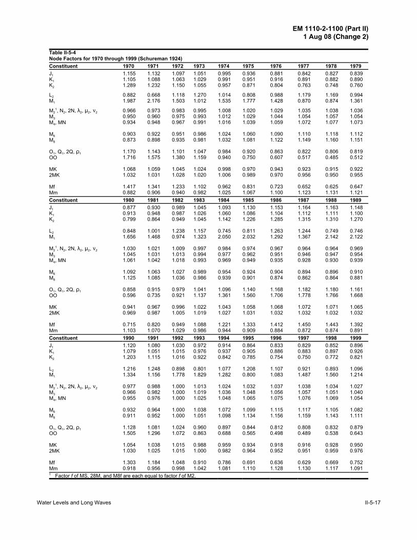
For example, the value for Hn in Equation II-5-16 is the mean constituent amplitude and is a function of bothlocation and variations arising from changes in the latitude of the moon’s node. The nodal effect of the moonis reflected by the introduction of the node factor fn, which modifies each constituent amplitude to correspondto a specific time period. Mid-year values are usually specified for reconstructed time series because nodefactors vary slowly in time. Mid-year values for each constituent listed in Table II-5-3 are presented inShureman (1924) for the years 1850 through 1999. An example is shown in Table II-5-4 for the years 1970through 1999. Equations for computing fn are given by Schureman.
(h) The second category of arguments specifies the phasing of high water for each constituent withrespect to both time and location. These arguments are based on the fact that phases of the constituents ofthe observed tide do not coincide with the phases of the corresponding constituents of the equilibrium tide.For example, a high tide does not occur directly beneath the moon. There is a lag between the location of thetide-producing force (i.e., location of the moon) and the observed time of high water. This lag, due tofrictional and inertial forces acting on the propagating tide, is referred to as the epoch of the constituent andis denoted by 6n in Equation II-5-16.
(i) The relationship between the constituent arguments and high tide is shown in the schematicFigure II-5-10. In this figure, the cosine curve represents the surface elevation in the y-direction as a functionof time or degrees of phase (maximum at 0 and 360 deg). For the M2 tidal constituent, the cosine curve hasa period of 12.42 hr (other constituent periods are indicated in Table II-5-3). Therefore, in Figure II-5-10,the horizontal axis represents either time or phase, both increasing to the right. The value of 6 represents theactual phase lag required for the water surface to reach high water (HW) following the passing of the tide-producing force. In the case of the semidiurnal constituents, this force is the crossing of the moon.

EM 1110-2-1100 (Part II)1 Aug 08 (Change 2)
II-5-16 Water Levels and Long Waves
Table II-5-3NOS Tidal Constituents and Arguments
Symbol Speed, deg/hr Period, hr Symbol Speed, deg/hr Period, hrM2 28.984 12.421 Mm 0.544 661.765
S2 30.000 12.000 Ssa 0.082 4390.244
N2 28.439 12.659 Sa 0.041 8780.488
K1 15.041 23.935 Msf 1.015 354.680
M4 57.968 6.2103 Mf 1.098 327.869
O1 13.943 25.819 D1 13.471 26.724
M6 86.952 4.140 Q1 13.398 26.870
(MK)3 44.025 8.177 T2 29.958 12.017
S4 60.000 6.000 R2 30.041 11.984
(MN)4 57.423 6.269 (2Q)1 12.854 28.007
<2 28.512 12.626 P1 14.958 24.067
S6 90.000 4.000 (2SM)2 31.015 11.607
:2 27.968 12.872 M3 43.476 8.280
(2N)2 27.895 12.906 L2 29.528 12.192
(OO)1 16.139 22.306 (2MK)3 42.927 8.386
82 29.455 12.222 K2 30.082 11.967
S1 15.000 24.000 M8 115.936 3.105
M1 14.496 24.834 (MS)4 58.984 6.103
J1 15.585 23.099
(j) The value 6 is approximately constant at every location in the world because it represents the actuallag between the passing of the tide-producing force (i.e., moon) at a specific location and the following high-tide contribution of that force at that same location. It is computed as the sum of the theoretical phase or timelead of the tide-producing force relative to the observer at some fixed time and the measured phase lag . fromthe observer at that fixed time to the following high water. The theoretical location of the tide-producing forceis referred to as the equilibrium argument (V0 + u). In Figure II-5-10, the tide-producing force andcorresponding equilibrium tide at location M are located (V0 + u) degrees ahead of point T. Conversely, theequilibrium tide will be located at point T if shifted (V0 + u) degrees. The value of . represents the phase lagfrom point T to HW.
(k) The equilibrium argument (V0 + u) is computed from equations defining the time-varying relationshipbetween the earth, moon, and sun. The value of . is computed from observed tidal time series data. Asstated, the sum of these two values is approximately constant for any fixed location at any time.
(l) Values of the equilibrium argument for the constituents of Table II-5-3 relative to the passing of thetidal potential force at the Greenwich meridian for each calendar year from 1850 through 2000 are tabulatedin Schureman (1924). An example is shown in Table II-5-5 for the years 1990 to 2000. Monthly and dailyadjustment tables are also presented. Each of the values is computed according to the respective constituentspeeds shown in Table II-5-3. The equilibrium arguments tabulated in Schureman are referenced to themeridian of Greenwich; therefore, the argument (V0 + u) represents the phase difference in degrees betweenthe location of the tidal potential term (moon or sun) and Greenwich relative to some specific time.
EM 1110-2-1100 (Part II)1 Aug 08 (Change 2)
Water Levels and Long Waves II-5-17
Table II-5-4Node Factors for 1970 through 1999 (Schureman 1924)Constituent 1970 1971 1972 1973 1974 1975 1976 1977 1978 1979J1K1K2
L2M1
M21, N2, 2N, 82, :2, <2
M3M4, MN
M6M8
O1, Q1, 2Q, D1OO
MK2MK
MfMm
1.1551.1051.289
0.8821.987
0.9660.9500.934
0.9030.873
1.1701.716
1.0681.032
1.4170.882
1.1321.0881.232
0.6682.176
0.9730.9600.948
0.9220.898
1.1431.575
1.0591.031
1.3410.906
1.0971.0631.150
1.1181.503
0.9830.9750.967
0.9510.935
1.1011.380
1.0451.028
1.2330.940
1.0511.0291.055
1.2701.012
0.9950.9930.991
0.9860.981
1.0471.159
1.0241.020
1.1020.982
0.9950.9910.957
1.0141.535
1.0081.0121.016
1.0241.032
0.9840.940
0.9981.006
0.9621.025
0.9360.9510.871
0.8081.777
1.0201.0291.039
1.0601.081
0.9200.750
0.9700.989
0.8311.067
0.8810.9160.804
0.9881.428
1.0291.0441.059
1.0901.122
0.8630.607
0.9430.970
0.7231.100
0.8420.8910.763
1.1790.870
1.0351.0541.072
1.1101.149
0.8220.517
0.9230.956
0.6521.123
0.8270.8820.748
1.1690.874
1.0381.0571.077
1.1181.160
0.8060.485
0.9150.950
0.6251.131
0.8390.8900.760
0.9941.361
1.0361.0541.073
1.1121.151
0.8190.512
0.9220.955
0.6471.121
Constituent 1980 1981 1982 1983 1984 1985 1986 1987 1988 1989J1K1K2
L2M1
M21, N2, 2N, 82, :2, <2
M3M4, MN
M6M8
O1, Q1, 2Q, D1OO
MK2MK
MfMm
0.8770.9130.799
0.8481.656
1.0301.0451.061
1.0921.125
0.8580.596
0.9410.969
0.7151.103
0.9300.9480.864
1.0011.468
1.0211.0311.042
1.0631.085
0.9150.735
0.9670.987
0.8201.070
0.9890.9870.949
1.2380.974
1.0091.0131.018
1.0271.036
0.9790.921
0.9961.005
0.9491.029
1.0451.0261.045
1.1571.323
0.9970.9940.993
0.9890.986
1.0411.137
1.0221.019
1.0880.986
1.0931.0601.142
0.7452.050
0.9840.9770.969
0.9540.939
1.0961.361
1.0431.027
1.2210.944
1.1301.0861.226
0.8112.032
0.9740.9620.949
0.9240.901
1.1401.560
1.0581.031
1.3330.909
1.1531.1041.285
1.2631.292
0.9670.9510.935
0.9040.874
1.1681.706
1.0681.032
1.4120.884
1.1641.1121.315
1.2441.367
0.9640.9460.928
0.8940.862
1.1821.778
1.0721.032
1.4500.872
1.1631.1111.310
0.7492.142
0.9640.9470.930
0.8960.864
1.1801.766
1.0711.032
1.4430.874
1.1481.1001.270
0.7462.122
0.9690.9540.939
0.9100.881
1.1611.668
1.0651.032
1.3920.891
Constituent 1990 1991 1992 1993 1994 1995 1996 1997 1998 1999J1K1K2
L2M1
M21, N2, 2N, 82, :2, <2
M3M4, MN
M6M8
O1, Q1, 2Q, D1OO
MK2MK
MfMm
1.1201.0791.203
1.2161.334
0.9770.9660.955
0.9320.911
1.1281.505
1.0541.030
1.3030.918
1.0801.0511.115
1.2481.156
0.9880.9820.976
0.9640.952
1.0811.296
1.0381.025
1.1840.956
1.0301.0151.016
0.8981.778
1.0001.0001.000
1.0001.000
1.0241.072
1.0151.015
1.0480.998
0.9720.9760.922
0.8011.829
1.0131.0191.025
1.0381.051
0.9600.863
0.9881.000
0.9101.042
0.9140.9370.842
1.0771.282
1.0241.0361.048
1.0721.098
0.8970.688
0.9590.982
0.7861.081
0.8640.9050.785
1.2080.800
1.0321.0481.065
1.0991.134
0.8440.565
0.9340.964
0.6911.110
0.8330.8860.754
1.1071.083
1.0371.0561.075
1.1151.156
0.8120.498
0.9180.952
0.6361.128
0.8290.8830.750
0.9211.487
1.0381.0571.076
1.1171.159
0.8080.489
0.9160.951
0.6291.130
0.8520.8970.772
0.8931.560
1.0341.0511.069
1.1051.143
0.8320.538
0.9280.959
0.6691.117
0.8960.9260.821
1.0961.214
1.0271.0401.054
1.0821.111
0.8790.643
0.9500.976
0.7521.091
1 Factor f of MS, 28M, and M8f are each equal to factor f of M2.

EM 1110-2-1100 (Part II)1 Aug 08 (Change 2)
II-5-18 Water Levels and Long Waves
Figure II-5-10. Tidal phase relationships
(m) A tidal simulation computer program is available in ACES (Leenknecht, Szuwalski, and Sherlock1992) to compute nodal factors and local (or Greenwich) equilibrium argument values for any time periodand generate the corresponding water surface time series as a function of input constituent amplitudes.Formulas for computing the equilibrium arguments are found in Shureman (1924), but are too lengthy for thismanual.
(3) Harmonic reconstruction.
(a) In order to reconstruct a tidal series for a specific time and location, the various phase argumentsof Equation II-5-16 must be defined according to local conditions. Generally, local values of 6n, H0, and Hnare available from NOS harmonic analyses. Because the values of the nodal factors fn are slowly varying,the yearly values determined according to Schureman are sufficiently accurate for the particular time ofinterest throughout the world. However, local values of (V0 + u)n vary with the speed of the constituent andhave to be determined for the location and time of interest. This information can be computed from tabulatedequilibrium arguments relative to Greenwich such as those presented in Schureman or computed withprograms developed for that purpose such as those contained in ACES.
(b) Values of the local equilibrium arguments, i.e., local (V0 + u)n, represent the instantaneous value ofeach of the equilibrium tide-producing force constituents (in degrees) with respect to some specific point onthe earth; for example, the time-varying location of the moon and sun with respect to some location on theearth. Referring to Figure II-5-11, the horizontal axis represents distance with the point G representingGreenwich, England, and O representing an observer located at some point west of Greenwich. The locationof the moon with respect to Greenwich at longitude 0o at Greenwich time t0 is indicated by the Greenwichequilibrium argument presented in Shureman, denoted as Greenwich (V0 + u), for time Greenwich t0.

EM 1110-2-1100 (Part II)1 Aug 08 (Change 2)
Water Levels and Long Waves II-5-19
Table II-5-5Equilibrium Argument for Beginning of Years 2001 through 2010
Constituent 2001 2002 2003 2004 2005 2006 2007 2008 2009 2010
J1 227.9 316.9 47.0 138.0 243.7 335.7 67.8 159.8 265.5 356.5K1 1.9 1.8 2.6 4.1 7.1 9.3 11.7 13.9 1 6.8 18.3K2 184.0 183.3 184.6 187.6 193.7 198.5 203.5 208.2 214.3 217.1L2 269.1 105.4 267.4 94.8 295.2 141.6 297.3 121.4 321.6 165.8M1 145.4 52.1 303.7 204.7 139.6 58.2 311.4 210.3 141.0 64.7
M2 210.8 311.4 52.4 153.5 230.4 331.9 73.4 174.8 251.7 352.9M3 316.1 287.1 258.5 230.2 165.7 137.8 110.0 82.2 17.6 349.3M4 61.5 262.9 104.7 307.0 100.9 303.8 146.7 349.6 143.5 345.7M6 272.3 214.3 157.1 100.5 331.3 275.6 220.1 164.4 35.2 338.6M8 123.1 165.7 209.4 254.0 201.7 247.5 293.4 339.2 286.9 331.4
N2 340.5 353.5 4.7 17.1 352.3 5.0 17.7 30.4 5.6 18.02N 110.3 33.5 317.0 240.7 114.1 38.1 322.1 246.1 119.5 43.1O1 213.0 313.5 53.0 151.8 224.9 323.0 61.2 159.3 232.4 331.3OO 322.4 222.3 125.6 31.5 326.3 234.6 143.3 51.6 346.3 251.9
P1 349.3 349.5 349.8 350.0 349.3 349.5 349.7 350.0 349.2 349.5Q1 342.8 354.6 5.3 15.5 346.7 356.1 5.5 15.0 346.3 356.42Q 112.6 35.6 317.7 239.0 108.5 29.2 309.9 230.6 100.1 21.5R2 177.8 177.5 177.3 177.0 177.7 177.5 177.2 177.0 177.7 177.4
S1 180.0 180.0 180.0 180.0 180.0 180.0 180.0 180.0 180.0 180.0S2,4,6 0.0 0.0 0.0 0.0 0.0 0.0 0.0 0.0 0.0 0.0T2 2.2 2.5 2.7 3.0 2.3 2.5 2.8 3.0 2.3 2.6
82 307.7 218.9 130.3 42.0 300.8 212.8 124.8 36.7 295.5 207.1:2 63.6 265.0 106.7 308.6 101.9 304.1 146.3 348.5 141.8 343.7<2 293.8 224.0 154.4 85.0 340.1 271.0 202.0 132.9 28.0 318.6D1 296.1 226.1 155.0 83.3 334.5 262.2 189.7 117.4 8.6 297.0
MK 212.6 313.2 54.9 157.6 237.5 341.2 85.0 188.7 268.6 11.12MK 59.6 261.1 102.1 302.9 93.8 294.4 135.1 335.7 126.6 327.4MN 191.3 303.9 57.0 170.6 222.7 336.9 91.1 205.2 257.3 10.9MS 210.8 311.4 52.4 153.5 230.4 331.9 73.4 174.8 251.7 352.92SM 149.2 48.6 307.6 206.5 129.6 28.1 286.6 185.2 108.3 7.1
Mf 324.7 224.4 126.3 29.8 320.7 225.8 131.0 36.1 326.9 230.3MSf 147.2 46.4 305.7 204.9 128.5 27.8 287.0 186.3 109.9 9.2Mm 230.2 318.9 47.7 136.4 238.2 326.9 55.6 144.3 246.1 334.9
Sa 280.7 280.5 280.2 280.0 280.8 280.5 280.3 280.0 280.8 280.5Ssa 201.4 201.0 200.5 200.0 201.5 201.0 200.5 200.1 201.6 201.1Methodology based on Schureman 1924. Values computed May 2001.
(c) The location of the moon at Greenwich time t0 is different for an observer at some point O locatedat longitude Lo than it is for the observer located at Greenwich. For each constituent, the observer is locatedpL deg from Greenwich; therefore, the local equilibrium argument must be adjusted by -pL to account for thedifference in location between the point of interest (i.e., point O) and Greenwich.
(d) The -pL adjustment provides the necessary equilibrium argument correction for differences inlocation between some point and Greenwich, i.e., a local equilibrium argument corresponding to an observerat location O. However, the value of the equilibrium argument Greenwich (V0 + u) was specified with respectto Greenwich t0. Therefore, Greenwich time must be written with respect to local time. Because local timefor the observer located west of Greenwich is earlier than local time in Greenwich (t0), the followingadjustment is made to convert local time to Greenwich time.

EM 1110-2-1100 (Part II)1 Aug 08 (Change 2)
II-5-20 Water Levels and Long Waves
Figure II-5-11. Phase angle argument relationship
(II-5-17)
where S is the local time meridian (shown on NOS analyses) and the number 15 indicates a time change of1 hr per 15 deg longitude.
(e) The speed of the time argument (ant in Equation II-5-16) in degrees with respect to time is equal tothe speed of the constituent an multiplied by Equation II-5-17. Therefore, the final relationship between localand Greenwich phase arguments that account for both differences in location (-pL) and local time (aS/15) canbe written as:
(II-5-18)
Therefore, a tide at any arbitrary location is computed as
(II-5-19)
(f) A reconstructed tidal time series of a published NOS harmonic analysis is presented for Sandy Hook,NJ. The NOS analysis is shown in Figure II-5-12. As can be seen by the reported amplitudes, the M2, S2, N2,K1, Sa, O1, <2, and K2 constituents contain the majority of the tidal energy. These constituents are used togenerate a 15-day tidal signal beginning on 1 January 1984 at 0000 hr Eastern Standard Time. Computedvalues are compared to the high and low tide predictions published in the Tide Tables for 1984 (NOAA 1984)shown in Figure II-5-13. Because all 37 constituents are not used in the reconstruction, the match is notperfect; however, it demonstrates the degree of accuracy that can be achieved by using only majorconstituents.

EM 1110-2-1100 (Part II)1 Aug 08 (Change 2)
Water Levels and Long Waves II-5-21
Figure II-5-12. NOS harmonic analysis for Sandy Hook, NJ

EM 1110-2-1100 (Part II)1 Aug 08 (Change 2)
II-5-22 Water Levels and Long Waves
Figure II-5-13. Tide tables for Sandy Hook, NJ (NOAA 1984)

EM 1110-2-1100 (Part II)1 Aug 08 (Change 2)
Water Levels and Long Waves II-5-23
(g) Reconstruction of the tide involves determining the equilibrium arguments, node factors, longitudeand time adjustment for each constituent, and using the published values for 6, Hn, and H0 in the NOSharmonic analysis. Table II-5-6 summarizes all necessary quantities.
Table II-5-6Harmonic Arguments for Sandy Hook NJ (1 January 1984 at 0000 hr)
Symbol G(V0+ u) pL aS/15 6 f H
M2 60.0 148.0 144.92 219.1 0.99 2.151
S2 0.0 148.0 150.00 246.0 1.00 0.448
N2 323.4 148.0 142.20 204.1 0.99 0.473
K1 2.4 74.0 75.20 102.2 1.04 0.319
Sa 279.8 0.0 0.20 128.7 1.00 0.254
O1 60.8 74.0 69.71 98.4 1.07 0.172
<2 148.0 148.0 142.56 191.1 0.99 0.109
K2 184.2 148.0 150.41 251.9 1.09 0.121
(h) The NOS harmonic analysis indicates that a multiplier of 1.04 should be used for all short-periodconstituents and that the value of H0 is 2.36 MSL. Also indicated on the analysis is the time meridian of 75°west longitude for use in computing the time zone compensation term aS/15. The 15-day tidal envelope isshown in Figure II-5-14. The open circles shown in the figure represent high- and low-water level predictionsextracted from the tide tables in Figure II-5-13. As stated, the comparison is not exact because only eightconstituents were used in the reconstruction. The match is, however, adequate for the majority of designapplications.
(i) The phase lag 6 in Equation II-5-19 is called the local epoch in order to distinguish it from otherforms of epochs (see Schureman (1924)). Some harmonic analyses use a modified form of the epoch thatautomatically accounts for the longitude and time meridian corrections. This modification is designated as6' and is defined as shown below
(II-5-20)
(j) This modified form is usually included on NOS harmonic analyses as indicated on Figure II-5-12.Use of this form of epoch in the reconstruction of tides is as shown below
(II-5-21)
(4) Tidal envelope classification.
(a) Semidiurnal, diurnal, and mixed tidal classifications were described in Part II-5-3a. Equation II-5-22is a more quantitative delineation of tide types.

EM 1110-2-1100 (Part II)1 Aug 08 (Change 2)
II-5-24 Water Levels and Long Waves
Figure II-5-14. Reconstructed tidal envelope for Sandy Hook, NJ
(II-5-22)
where A(K1), A(O1), A(M2), and A(S2) represent the amplitudes of the corresponding constituents. A generalclassification of tides can be separated according to the following criteria:
R # 0.25 Semidiurnal0.25 < R # 1.50 Mixed1.50 < R Diurnal
(b) The tidal classification for the Sandy Hook, NJ, example can be computed as shown below:
(II-5-23)
(c) According to the classification criteria, the tides at Sandy Hook are semidiurnal. In fact, most tidesalong the northern east coast of the United States are semidiurnal. Tides in the lower east coast and Gulf ofMexico begin to change from semidiurnal, to mixed, to diurnal as shown in Figure II-5-15.
EM 1110-2-1100 (Part II)1 Aug 08 (Change 2)
Water Levels and Long Waves II-5-25
Figure II-5-15. Areal extent of tidal types (Harris 1981)
c. Glossary of tide elevation terms.
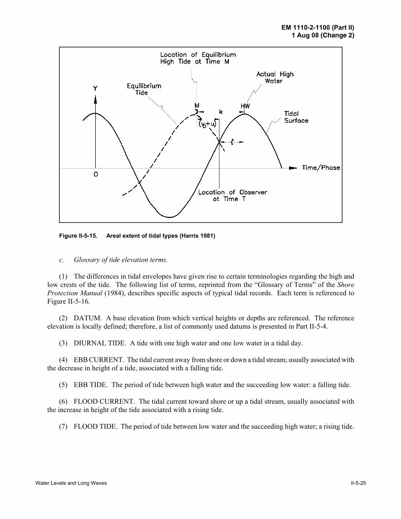
(1) The differences in tidal envelopes have given rise to certain terminologies regarding the high andlow crests of the tide. The following list of terms, reprinted from the “Glossary of Terms” of the ShoreProtection Manual (1984), describes specific aspects of typical tidal records. Each term is referenced toFigure II-5-16.
(2) DATUM. A base elevation from which vertical heights or depths are referenced. The referenceelevation is locally defined; therefore, a list of commonly used datums is presented in Part II-5-4.
(3) DIURNAL TIDE. A tide with one high water and one low water in a tidal day.
(4) EBB CURRENT. The tidal current away from shore or down a tidal stream; usually associated withthe decrease in height of a tide, associated with a falling tide.
(5) EBB TIDE. The period of tide between high water and the succeeding low water: a falling tide.
(6) FLOOD CURRENT. The tidal current toward shore or up a tidal stream, usually associated withthe increase in height of the tide associated with a rising tide.
(7) FLOOD TIDE. The period of tide between low water and the succeeding high water; a rising tide.

EM 1110-2-1100 (Part II)1 Aug 08 (Change 2)
II-5-26 Water Levels and Long Waves
Figure II-5-16. Types of tides (Shore Protection Manual 1984)

EM 1110-2-1100 (Part II)1 Aug 08 (Change 2)
Water Levels and Long Waves II-5-27
(8) HIGHER HIGH WATER (HHW). The higher of the two high waters of any tidal day. The singlehigh water occurring daily during periods when the tide is diurnal is considered to be a higher high water.
(9) HIGHER LOW WATER (HLW). The higher of two low waters of any tidal day.
(10) HIGH TIDE, HIGH WATER (HW). The maximum elevation reached by each rising tide.
(11) LOW TIDE, LOW WATER (LW). The minimum elevation reached by each falling tide.
(12) LOWER HIGH WATER (LHW). The lower of the two high waters of any tidal day.
(13) LOWER LOW WATER (LLW). The lower of the two low waters of any tidal day. The single lowwater occurring daily during periods when the tide is diurnal is considered to be a lower low water.
(14) MIXED TIDE. A tide in which the presence of a diurnal wave is conspicuous due to a largeinequality in either the high or low water heights, with two high waters and two low waters usually occurringeach tidal day. In strictness, all tides are mixed, but the name is usually applied without definite limits to thetide intermediate to those predominantly semidiurnal and those diurnal.
(15) SEMIDIURNAL TIDE. A tide with two high and two low waters in a tidal day with comparativelylittle diurnal inequality.
(16) TIDAL DAY. The time of the rotation of the earth with respect to the moon, or the interval betweentwo successive upper transits of the moon over the meridian of a place, approximately 24.84 solar hours(24 hr and 50 min) or 1.035 times per solar day. Also called a lunar day.
(17) TIDAL PERIOD. The interval of time between two consecutive, like phases of the tide.
(18) TIDAL RANGE. The difference in height between consecutive high and low (or higher high andlower low) waters.
(19) TIDAL RISE. The height of the tide as referenced to the datum of a chart.
II-5-4. Water Surface Elevation Datums
a. Introduction. Water level and its change with respect to time have to be measured relative to somespecified elevation or datum in order to have a physical significance. In the fields of coastal engineering andoceanography this datum represents a critical design parameter because reported water levels provide anindication of minimum navigational depths or maximum surface elevations at which protective levees orberms are overtopped. It is therefore necessary that coastal datums represent some reference point which isuniversally understood and meaningful, both onshore and offshore. Ideally, two criteria should be expectedof a datum: 1) that it provides local depth of water information, and 2) that it is fixed regardless of locationsuch that elevations at different locations can be compared. These two criteria are not necessarily compatible.The following list of datums represents those commonly in use in the United States.
b. Tidal-observation-based datums.
(1) Tidal-observation-based datums are computed from measured time series of tidal elevations. Assuch, they vary with geographical location and exposure. Geographic variability of tide records can be seenin Figures II-5-8 and II-5-9. Although datums based on tidal series do indicate site-specific conditions, they

EM 1110-2-1100 (Part II)1 Aug 08 (Change 2)
II-5-28 Water Levels and Long Waves
may not be comparable with similar measurements at other geographic locations because of the difficulty ofassigning a comparable gauge zero. The most widely accepted of the datums computed from time series aredescribed below.
(2) Mean sea level (MSL) was widely adopted as a primary datum on the assumption that it could beaccurately computed from tidal elevation records measured at any well-exposed tide gauge. MSLdeterminations are based on the arithmetic average of hourly water surface elevations observed over a longperiod of time. The ideal length of record is approximately 19 years, a period that accounts for the 18- to 19-year long-term cycle in tides and is sufficient to remove most meteorological effects. In order to fix thedatum in time for a specific location, a common 19-year period is selected for computing MSL. The specific19-year cycle was adopted by the National Ocean Survey as the official time segment for use in computingmean values for tidal datums. The 19-year period, called the National Tidal Datum Epoch, is updatedapproximately every 25 years.
(3) When estimates of MSL are required, but less than 19 years of data are available, computationsshould be based on an integral number of tidal cycles, for example, an integral number of years or 29-dayspring/neap cycles. For gauges where hourly data are not available, or their use is impractical, MSL can beapproximated as the tidal datum midway between MHW and MLW. This datum, referred to as Mean TideLevel (MTL), may differ from MSL depending on the local relative importance of the diurnal componentsof the tide.
(4) Alternate tidal datums are based on low water tidal elevations. These datums provide minimumdepth information for navigational needs. Two commonly used low-water datums in the United States arethe Mean Low Water (MLW) for the Atlantic Coast and the Mean Lower Low Water (MLLW) for the Pacificcoast. The MLLW datum is currently being adopted to several locations along the Atlantic coast. Bothdatums are defined as the average tidal height at low water or lower low water during the 19-year period.Additional datums, applicable to specific locations or purposes, include Mean High Water (MHW) and MeanHigher High Water (MHHW). These are derived in a manner similar to MLW and MLLW. For areas ofprimarily semidiurnal tides, the difference between MHW and MLW is called the mean tidal range. Thedifference between MHHW and MLLW gives a corresponding diurnal range or the great diurnal range of thetide. Both numbers provide an estimate of the magnitude of the local tidal range. An example of thevariability of the above datums is given by Harris (1981) and reproduced in Table II-5-7. Reference tidestations used in the preparation of Table II-5-7 are shown in Figure II-5-17.
c. 1929 NGVD datum.
(1) One difficulty with using any of the observation-based datums described above is that they varyconsiderably with location, as evidenced in Table II-5-7. Also, because each datum can be computedindependently, there is little or no connectivity between datum locations. This lack of a reference elevationfor areas near the coast where no tide observations are available and at interior locations where tideobservations are difficult to obtain led to the establishment of a national fixed datum. This datum does notaccount for spatial variability in sea level. The following paragraphs describe the development of the 1929National Geodetic Vertical Datum (NGVD).
(2) First-order leveling lines established in the mid-1920’s provided survey connections between theAtlantic and Pacific coasts. These surveys indicated that sea levels were higher on the Pacific coast than onthe Atlantic coast and were also higher in the north than in the south on both coasts. The goal of developinga fixed reference datum was accomplished by defining a geodetic leveling-based datum whose “zero”coincided with local MSL at locations at which both MSL and geodetic leveling elevations were known.

EM 1110-2-1100 (Part II)1 Aug 08 (Change 2)
Water Levels and Long Waves II-5-29
Table II-5-7Datums for Reference Tide Stations (Harris 1981)
Extremes of Record
StationNormalizingFactor2 MSL MTL NGVD MLLW MLW MHW MHHW Highest Lowest
Interval forEstablishingof Datum
Atlantic and Gulf CoastsEastport, Maine M 9.2 9.10 9.00 --3 0.00 18.20 --3 23.1 -4.4 1941-61Portland, Maine M 4.5 4.50 4.28 0.00 9.00 13.9 -3.7 1941-59Boston, Mass. M 5.2 5.05 4.89 0.304 9.80 14.2 -3.5 1941-59Newport, R.I. M 1.6 1.75 1.37 0.00 3.50 13.5 -2.9 1941-59New London, Conn. M 1.4 1.30 0.97 0.00 2.60 10.75 -3.4 1941-59Bridgeport, Conn. M 3.4 3.35 2.86 0.00 6.70 12.4 -3.55 1967 (1 yr)Willets Point, N.Y. M 3.6 3.55 3.02 0.00 7.10 16.7 -4.1 1941-59New York, N.Y.(The Battery) M 2.3 2.25 1.81 0.00 4.50 10.2 -4.2 1941-59Albany, N.Y. M 2.5 2.5 --6 0.00 4.60 --6 --6 1941-59Sandy Hook, N.J. M 2.3 2.30 1.79 0.00 4.60 10.3 -4.4 1941-59Breakwater Harbor, Del. M 2.1 2.05 1.69 0.00 4.10 9.5 -3.9 1953-61Reedy Point, Del. M 2.8 2.75 2.45 0.00 5.50 10.05 -6.3 1957-61Philadelphia, Pa. M 3.2 3.10 2.14 0.00 6.197 10.7 -6.6 1941-59Baltimore, Md. M 1.0 0.97 0.57 0.428 1.52 8.3 -4.5 1941-59Washington, D.C. M 1.97 1.97 1.43 0.529 3.42 11.9 -4.2 1941-59Hampton Roads, Va. (Sewells Point) M 1.3 1.25 1.28 0.00 2.50 8.5 -3.1 1941-59
Wilmington, N.C. M 1.9 2.10 1.52 0.00 4.20 8.2 -1.7Jan. 1969 to Nov. 1973
Charleston, S.C. M 2.7 2.91 2.65 0.3110 5.51 10.7 -3.3 1941-59Savannah River Entrance, Ga. (Ft. Pulaski) M 3.6 3.45 3.32 0.00 6.90 11.1 -4.4 1941-59Savannah, Ga. M 4.0 3.7 --6 0.00 7.40 --6 --6 1941-59Mayport, Fla. M 2.3 2.25 2.00 0.00 4.50 7.4 -3.2 1941-59Miami Harbor Entrance, Fla. M 1.3 1.25 0.96 0.00 2.50 6.4 -1.6 1941-59Key West, Fla. M 0.6 0.65 0.42 0.00 1.30 3.8 -1.6 1941-59St. Petersburg, Fla. D 1.2 1.15 0.83 0.00 2.30 5.3 -2.55 1941-59 1 Except as footnoted, chart datum is MLW for the Atlantic and gulf coasts and MLLW for the Pacific coast. 2 D = diurnal; M = mean. 3 MLLW and MHHW were not routinely derived for Atlantic and gulf coast stations for the 1941-59 epoch used for establishing most of thedatums. 4 Boston Low Water Datum (adopted about 1927). 5 Estimated value. 6 Data unavailable at the time of compilation. 7 Datums and the mean range for Philadelphia were revised in July 1979 based on observations for the period 1969-77. 8 Baltimore Low Water Datum (adopted 1922 by NOS and COE based on observations 1903-1921). 9 Mean River Level.10 Charleston Low Water Datum (used since 1905 by NOS, and by COE in May 1929).11 Low Water Datum at the Presidio, Golden Gate, San Francisco, is based on miscellaneous observations before 1907.
(Continued)

EM 1110-2-1100 (Part II)1 Aug 08 (Change 2)
II-5-30 Water Levels and Long Waves
Table II-5-7 (Concluded)Extremes of Record
StationNormalizingFactor2 MSL MTL NGVD MLLW MLW MHW MHHW Highest Lowest
Interval forEstablishingof Datum
Atlantic and Gulf Coasts (Continued)
St. Marks River Entrance, Fla. D 1.8 1.8 --6 0.00 2.40 8.0 -3.5 1941-59Pensacola, Fla. D 0.6 0.65 0.33 0.00 1.30 8.9 -2.2 1941-59Mobile, Ala. D 0.8 0.75 --6 0.00 1.50 9.05 -3.05 1941-59Galveston, Tex. (Ship channel) D 0.8 0.70 0.70 0.00 1.40 11.4 -5.3 1941-59
San Juan, P.R. D 0.6 0.55 --6 0.00 1.10 2.4 -1.1Apr. 1962 to Dec. 1963
Pacific CoastSan Diego, Calif. D 3.0 2.95 2.79 0.00 0.90 5.00 5.70 8.3 -2.8 1941-59Los Angeles, Calif.(Outer Harbor) D 2.8 2.80 2.72 0.00 0.90 4.70 5.40 7.8 -2.6 1941-59San Francisco, Calif.(Golden Gate) D 3.0 3.30 3.06 0.2011 1.30 5.30 5.90 8.6 -2.5 1941-59Humboldt Bay, Calif D 3.4 3.75 -- 0.00 1.20 5.70 6.40 9.55 -3.05 1962Astoria, Oreg.(Tongue Point)9 D 4.3 4.35 3.05 0.00 1.10 7.60 8.30 12.1 -2.8 1941-59Aberdeen, Wash. D 5.5 5.45 -- 0.00 1.50 9.40 10.10 14.9 -2.9 1955, 1956Port Townsend,Wash. D 4.8 5.10 -- 0.00 2.50 7.70 8.40 12.05 -4.55 1972-74Seattle, Wash. D 6.6 6.60 6.25 0.00 2.80 10.40 11.30 14.8 -4.7 1941-59Ketchikan, Alaska D 8.0 7.95 -- 0.00 1.50 14.40 15.30 21.2 -5.2 1941-59Juneau, Alaska D 8.6 8.50 -- 0.00 1.60 15.40 16.40 23.2 -5.2 1966-72Sitka, Alaska D 5.2 5.30 -- 0.00 1.40 9.10 9.90 14.6 -3.8 1941-59Cordova, Alaska D 6.6 6.45 -- 0.00 1.40 11.50 12.40 16.8 -4.9 1965-74Seldovia, Alaska D 9.4 9.35 -- 0.00 1.60 17.00 17.80 24.3 -6.2 1971-74Anchorage, Alaska D 16.8 15.25 -- 0.00 2.20 28.30 29.00 35.55 -6.55 1964-68Kodiak, Alaska D 4.3 4.30 -- 0.00 1.00 7.60 8.50 13.05 -4.05 1935-36Dutch Harbor, Alaska D 2.2 1.30 -- 0.00 1.20 3.40 3.70 6.6 -2.7 1935-38Sweeper Cove,Alaska (Adak Island) D 2.1 1.85 -- 0.00 -- -- 3.70 7.05 -3.3
1958-60;1944, 1949
Massacre Bay, Alaska(Attu Island) D 1.9 1.65 -- 0.00 -- -- 3.30 7.05 -3.05
1950, 1952,1960
Nashagak Bay, Alaska(Clarks Pt) D 10.3 10.15 -- 0.00 2.50 17.80 19.50 24.5 -5.0 1958St. Michael, Alaska D 2.0 -- -- -- -- -- -- -- -- --Honolulu, Hawaii D 0.8 0.80 -- 0.00 0.20 1.40 1.90 3.5 -1.3 1941-59

EM 1110-2-1100 (Part II)1 Aug 08 (Change 2)
Water Levels and Long Waves II-5-31
Figu
re II
-5-1
7.
Ref
eren
ce a
nd c
ompa
rativ
e tid
e st
atio
ns, A
tlant
ic, G
ulf,
and
Paci
fic c
oast
s (H
arris
198
1)

EM 1110-2-1100 (Part II)1 Aug 08 (Change 2)
II-5-32 Water Levels and Long Waves
Thus, a general adjustment was made in 1929 in which it was assumed that the geodetic and local sea levelswere equal to zero at 26 selected tide gauges in the United States and Canada (Rappleye 1932). Thedifferences previously computed were treated as errors and were distributed over the network of observationpoints (Harris 1981). The tide gauge locations used in this computation are shown in Figure II-5-18. Thedatum, originally called the “Sea Level Datum of 1929,” was officially renamed the “National GeodeticVertical Datum (NGVD) of 1929” in 1963.
(3) Index maps of tidal benchmarks and lists of established references between the 1929 NGVD andthe local MSL are available for each coastal state through the NOS. An NOS tidal benchmark sheet is shownin Figure II-5-19. These sheets often describe several benchmarks established in the vicinity of each tidalobservation point and describe the relationship between the various datums common to the area. NGVD andtidal benchmarks are discussed more thoroughly in Harris (1981).
(4) The primary distinction between the NGVD and all other tidal datums is that the NGVD is definedas a fixed surface whose elevation does not change with time. Therefore, the procedure adopted to accountfor recognized changes in relative mean sea level is to compute updated MSL (or other) datum relationships. Relative changes in sea level will be discussed in the following section.
d. Great Lakes datums.
(1) A separate water surface elevation datum was established for the Great Lakes basin and St.Lawrence River. The datum was originally established by an international coordination committee composedof representatives of the U.S. Army Corps of Engineers, the National Oceanic and AtmosphericAdministration, and the Department of the Environment, Canada. This first datum was called theInternational Great Lakes Datum (IGLD) of 1955. The “zero” of the datum was established as the averageof all hourly water surface water level readings at Pointe-au-Pere, Quebec, located on the Gulf ofSt. Lawrence for the period between 1941 and 1956.
(2) First-order leveling lines from Pointe-au-Pere were used to systematically define datums for LakeOntario, Lake Erie, Lakes Michigan and Huron, and Lake Superior. Lakes Michigan and Huron are assumedto have the same elevation because of the deep and wide connection of both lakes at the Straits of Mackinac.The IGLD of 1955 was replaced by the IGLD of 1985 to reflect certain corrections to the elevations assignedto the various lakes. Elevations of the IGLD of 1955 and IGLD of 1985 are given in Table II-5-8. Thisrevision was implemented in January 1992. The zero reference of the IGLD 1985 has been specified to beRimouski, Quebec. Revised lake elevations are shown in Figure II-5-20.
e. Long-term variations in datums. Water level observation based datums such as MSL or IGLD varyover time periods much longer than a tidal cycle. These variations can be seasonal or of much longerduration. Long-term changes are often described as a relative change in sea level and necessitate the 25-yearinterval updating of the 19-year tidal datum period. In the following section, some of the contributing factorsto sea level change are discussed. In the final section, factors contributing to long-term elevation changesin the Great Lake are presented.
f. Tidal datums.
(1) The apparent rise in worldwide sea level has been of great concern to the United States, as well asother countries, for several years. Much of this concern stems from the claims of some climatologists andoceanographers that the rise will accelerate in the future due to warming of the atmosphere associated withthe “greenhouse effect,” a global warming produced by increased levels of carbon dioxide and other gassesin the atmosphere. Because of the potential consequences associated with sea level rise, a Committee on
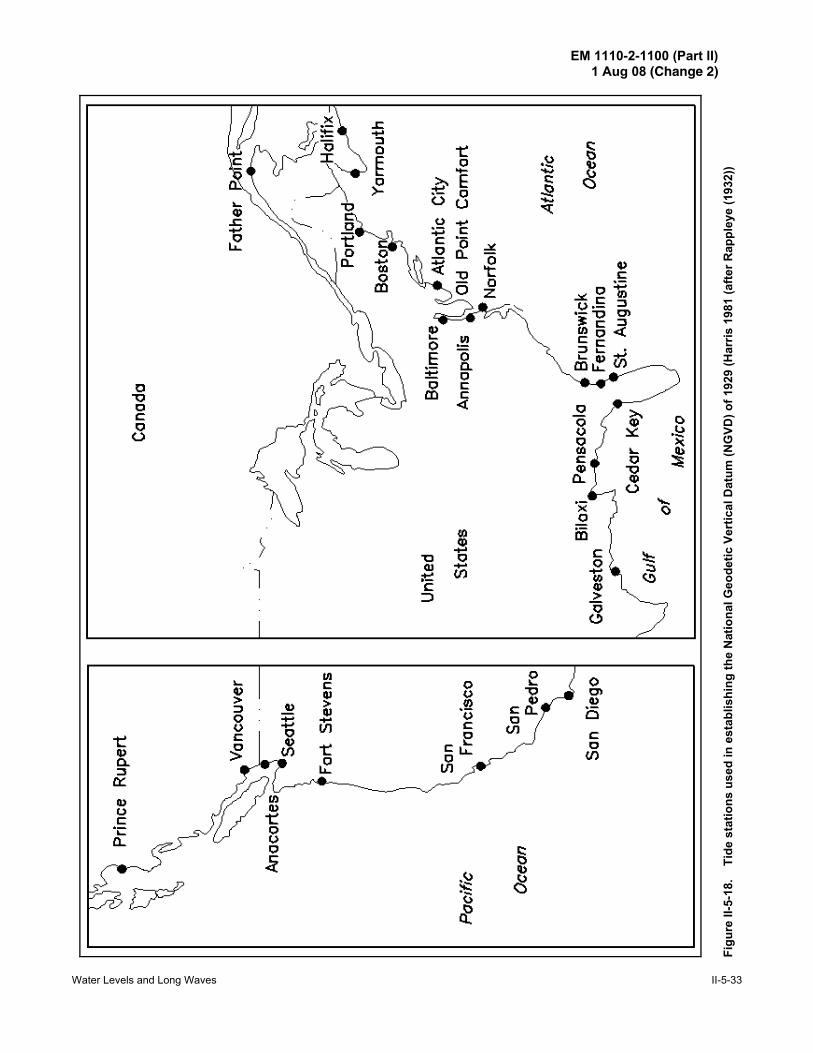
EM 1110-2-1100 (Part II)1 Aug 08 (Change 2)
Water Levels and Long Waves II-5-33
Figu
re II
-5-1
8.
Tid
e st
atio
ns u
sed
in e
stab
lishi
ng th
e N
atio
nal G
eode
tic V
ertic
al D
atum
(NG
VD) o
f 192
9 (H
arris
198
1 (a
fter R
appl
eye
(193
2))

EM 1110-2-1100 (Part II)1 Aug 08 (Change 2)
II-5-34 Water Levels and Long Waves
FLORIDA - I - 74
U.S. DEPARTMENT OF COMMERCENATIONAL OCEANIC AND ATMOSPHERIC ADMINISTRATION
NATIONAL OCEAN SURVEY
TIDAL BENCH MARKS
Miami Beach (City Pier)Lat. 25° 46N.1; Long 80° 07N.9
BENCH MARK 4 (1928) is a standard disk, stamped “NO 4 1928", set vertically in the south face of the south post in the north-south fence line around a large city water tank. It is about 66 feet north of the extended centerline of Commerce Street, 36 feet west of thecenterline of Jefferson Avenue, and 1/2 foot above ground level. Elevation: 5.62 feet above mean low water.
BENCH MARK 6 (1931) is a standard Corps of Engineers disk, stamped “BM NO 6,” set in top of a 2-inch pipe surrounded attop with a 12-inch by 18-inch manhole frame with a removable cast iron cover, directly in centerline of a blacktop driveway which parallelsGovernment Cut. It is at the U.S. Government Reservation on the north side of Government Cut, about 186 feet east of U.S. Engineersflagpole and 13 1/2 feet west of the center of a road junction. Elevation: 7.13 feet above mean low water.
BENCH MARK 7 (1937) is a standard disk, stamped “7 1937,” set in the top of the northwest side of the concrete base to theeast post of entrance gate to drive to the Corps of Engineers Office Building. It is about 100 yards south of intersection of WashingtonAvenue and Biscayne Street, 8 feet east of the extended centerline of the Avenue and 1/2 foot above ground level. Elevation: 5.03 feetabove mean low water.
BENCH MARK 9 (1955) is a standard disk, stamped “9 1955,” set in top of concrete deck along north edge of City Pier near theeast end of Biscayne Street. It is about 122 yards east of the west end of pier, 39 feet northwest of the northeast corner of the ladies restroom and 1/2 foot south of south face of north guardrail. Elevation: 11.29 feet above mean low water.
BENCH MARK 10 (1956) is a standard disk, stamped “NO 10 1956,” set on top of the northwest corner of the concrete base oflight pole No. 166D6 about 68 yards west of the junction of Biscayne Street and Alton Road. It is near the northwest corner of the SouthShore Recreation Park about 62 feet east of the west edge of the bulkhead on the water front and 9 1/2 feet northeast of the east edge of thenorth entrance to the Recreation Building. Elevation: 5.23 feet above mean low water.
BENCH MARK 11 (1956) is a standard disk, stamped “NO 11 1956,” set in top of north corner of a concrete base whichsupports a 6 inch metal post near the City of Miami Beach Warehouse. It is near the intersection of Alton Road and First Street about 21 1/2feet southwest of the southwest curb of Alton Road and 9 feet northwest of the northwest corner of the warehouse building. Elevation: 4.92feet above mean low water.
Mean low water at Miami Beach is based on 19 years of records, 1941-1959. Elevations of other tide planes referred to thisdatum are as follows:
FeetHighest tide (observed)
September 8, 1965 6.4Mean high water 2.50Mean tide level 1.25NGVD, 1929 0.96Mean low water 0.00Lowest tide observed
(March 24, 1936) -1.6
Figure II-5-19. Sample NOS description of tidal benchmarks (Harris 1981)

EM 1110-2-1100 (Part II)1 Aug 08 (Change 2)
Water Levels and Long Waves II-5-35
Figure II-5-20. Vertical and horizontal relationships for the IGLD of 1985 (Coordinating Committee on GreatLakes Basic Hydraulic and Hydrologic Data 1992)
Table II-5-8Low Water (chart) Datum for IGLD 1955 and IGLD 1985
Low Water Datum in Meters
Location IGLD 55 IGLD 85
Lake Superior 182.9 183.2
Lake Michigan 175.8 176.0
Lake Huron 175.8 176.0
Lake St. Clair 174.2 174.4
Lake Erie 173.3 173.5
Lake Ontario 74.0 74.2
Lake St. Lawrence at Long Sault Dam, Ontario 72.4 72.5
Lake St. Francis at Summerstown, Ontario 46.1 46.2
Lake St. Louis at Pointe Claire, Quebec 20.3 20.4
Montreal Harbour at Jetty Number 1 5.5 5.6

EM 1110-2-1100 (Part II)1 Aug 08 (Change 2)
II-5-36 Water Levels and Long Waves
Engineering Implications of Changes in Relative Mean Sea Level (CCMSL) was formed to examine existingknowledge concerning sea level change, to document existing relative rise rates, and to provide recommenda-tions concerning their conclusions.
(2) Relative mean sea level change can be defined as the difference between local changes in landelevation and global sea level changes. These changes result from a variety of processes, several of whichcan occur simultaneously. The following six processes can contribute to long-term relative mean sea levelchange; however, all processes do not necessarily apply to all geographic locations:
(a) Eustatic rise. Refers to a global change in the oceanic water level. Examples of eustatic rise includemelting of land-based glaciers and the expansion of near-surface ocean water due to global ocean warming.
(b) Crustal subsidence or uplift from tectonic uplifting or downwarping of the earth's crust. Thesechanges can result from uplifting or cooling of coastal belts, sediment loading and consolidation, orsubsidence due to volcanic eruption loading.
(c) Seismic subsidence. Caused by sudden and irregular incidence of earthquakes.
(d) Auto-subsidence. Due to compaction or consolidation of soft underlying sediments such as mudor peat.
(e) Climatic fluctuations. May also create changes in sea level; for example, surface changes producedby El Niño due to changes in the size and location of high pressure cells.
(3) The above processes have been evaluated with respect to their historical and potential contributionto sea level change on U.S. coasts. The Committee report assesses changes in sea level as well as the affectedhydrodynamic processes and the effect on the coastal zone. The report also investigates feasible responsestrategies that could be used to mitigate the effects of sea level change. Although it is beyond the scope ofthis chapter to reproduce the contents of the report, conclusions relevant to this chapter are reproduced below.
(a) Relative mean sea level, on statistical average, is rising at the majority of tide gauge stations situatedon continental coasts around the world. Relative mean sea level is generally falling near geological plateboundaries and in formerly glaciated areas such as Alaska, Canada, Scandinavia, and Scotland. Relativemean sea level is not rising in limited areas of the continental United States, including portions of the PacificCoast.
(b) The contrasting signals concerning relative mean sea level behavior in different parts of the UnitedStates (and the world in general) are interpreted as due to differing rates of vertical motion of the landsurfaces. Subsidence and glacial rebound are significant contributors to vertical land displacements.
(c) Large, short-term (2- to 7-year) fluctuations worldwide are related to meteorological phenomena,notably shifts in the mean jet-stream path and the El Niño-Southern Oscillation mechanisms, which lead toatmospheric pressure anomalies and temperature changes that may cause rise or fall of mean sea level by 15-30 cm over a few years.
(d) Studies of a very small number of tide gauge records dating more than 100 years (the oldest beingAmsterdam, started in 1682) show that after removal of the subsidence factor where known, mean sea levelhas been fluctuating through a range of not more than 40-150 cm (in long-term fluctuations) for at least 300years.
(e) The geological record over the last 6,000 years or so indicates that there has been a general, long-term rise (with short-term fluctuations) probably not exceeding 200 cm during the last 1,500 years.

EM 1110-2-1100 (Part II)1 Aug 08 (Change 2)
Water Levels and Long Waves II-5-37
(f) Monitoring of relative mean sea level behavior is at present inadequate for measuring the possibleglobal result of future climate warming due to rising greenhouse gases.
(g) The risk of accelerated mean sea level rise is sufficiently established to warrant consideration in theplanning and design of coastal facilities. Although there is substantial local variability and statisticaluncertainty, average relative sea level over the past century appears to have risen about 30 cm relative to theeast coast of the United States and 11 cm along the west coast, excluding Alaska, where glacial rebound hasresulted in a lowering of relative sea level. Rates of relative sea level rise along the Gulf Coast are highlyvariable, ranging from a high of more than 100 cm/century in parts of the Mississippi delta plain to a low ofless than 20 cm/century along Florida's west coast.
(h) Accelerated sea level rise would clearly contribute toward a tendency for exacerbated beach erosion.However, in some areas, poor sand management practices or navigational modification at channel entranceshas resulted in augmented erosion rates that are clearly much greater than would naturally occur. Thus, forsome years into the future, sea level rise may play a secondary role in these areas.
(i) As noted previously, the two response options to sea level rise are stabilization and retreat. Retreatis most appropriate in areas with a low degree of development. Given that a “proper” choice exists for eachlocation, selecting an incorrect response alternative could be unduly expensive.
(j) There does not now appear to be reason for emergency action regarding engineering structures tomitigate the effects of anticipated increases in future eustatic sea level rise. Sea level change during thedesign service life should be considered along with other factors, but it does not present such essentially newproblems as to require new techniques of analysis. The effects of sea level rise can be accommodated duringmaintenance periods or upon redesign and replacement of most existing structures and facilities. There arevery limited geographic areas where current subsidence rates may require near-term action as has been thecase in Japan and Terminal Island, California.
(4) The above conclusions represent the state of knowledge on the subject of relative sea level change.For additional information, the reader is referred to the Committee report. It presents a complete andcomprehensive investigation of the subject based on known facts and engineering and scientific principles.
(5) For the purposes of this report, the primary conclusion is that, with some regional exceptions, sealevel is not rising at a rate to cause undue concern. Results of the report indicate an average sea level riseover the past century of approximately 30 cm/century on the east coast, and 11 cm/century on the west coast,and a range along the Gulf of Mexico coast of less than 20 cm/century along the west coast of Florida to morethan 100 cm/century in parts of the Mississippi delta plain. The above summary remarks lead to theconclusion that normal design criteria should be followed in which the design life of a project should considerthe possible local relative sea level rise rates shown above.
g. Changes in lake level datums. As with long-term change in the relative mean sea level of theoceans, lake levels also change in time. Although lake levels are subject to the same tectonic types of relativemovement, the primary form of change is due to shorter-term phenomena. For example, lake levels aresubject to seasonal and annual variations in precipitation and freshwater inflow resulting from regulatedreservoirs. These hydrologically related effects produce water surface elevations in the Great Lakes that varyirregularly from one year to the next. The annual cycle consists of water surfaces that consistently fall inelevation to their lowest stage during winter. Falling stages are due to the fact that the majority ofprecipitation is in the form of snow or rainfall that freezes before becoming spring runoff into streams thatempty into the lakes. Lake levels then begin to rise in the spring as the snow and ice melt into runoff. Lakelevels generally reach their maximum during the summer. These long-term changes were the basis of therevised IGLD of 1985 described in the previous section.

EM 1110-2-1100 (Part II)1 Aug 08 (Change 2)
II-5-38 Water Levels and Long Waves
h. Design considerations.
(1) The datums described above and the reported variability of those datums represent design criteriaconsiderations that directly impact the expected lifetime of a project. If, for example, a coastal project is tobe situated in an area of known subsidence, then design elevations need to reflect additional freeboard as afactor-of-safety consideration. For example, if levee systems are to be situated in an area of knownsubsidence (i.e., the Gulf coast) and a crest elevation level of 20 ft NGVD is considered a minimum level ofprotection, the subsidence rate should be included in the design calculations to provide adequate protectionfor the life of the project. For example, if the relative sea level change is 1 cm/year, then the levee willsubside by approximately 1 ft in 30 years. This rate of change should be accounted for in the design ofprojects expected to provide some predetermined level of protection. In this case, the levee should bedesigned with a 21-ft NGVD crest elevation if it is intended to provide a minimum of 20 ft MSL (presenttime) protection for 30 years.
(2) If a design project needs to consider the possibility of long-term water level change, then accuratesources of data must be obtained for use in the design evaluation. The NOS continuously summarizesmonthly MSL values, the mean and extreme high and low waters of the month, and many other tidal statistics.These records can be obtained from NOS in the form of either photocopies or magnetic media. Figure II-5-21is a sample of NOS tide and sea level data. If data are available for a specific project location for a longperiod of time (i.e., 30-50 years), then relative sea level change rates for project design can be estimated. Forexample, plotted variations in annual sea level for several locations are shown in Figure II-5-22. These datacan be used to indicate relative sea level change.
(3) Although relative water surface elevations and datum changes are important over the life of aproject, it is usually the short-term changes in water surface elevations that are responsible for project failure(although sudden elevation changes due to tectonic influence can be catastrophic). These short-term changesto elevation are the subject of the following sections.
II-5-5. Storm Surge
a. Storm types. Storms are atmospheric disturbances characterized by low pressures and high winds. Astorm surge represents the water surface response to wind-induced surface shear stress and pressure fields.Storm-induced surges can produce short-term increases in water level that rise to an elevation considerablyabove mean water levels. This is especially true when the storm front coincides with a local high spring tide.There are two types of storms that impact coastal regions. Storms that originate in the tropics are referredto as “tropical storms.” These events primarily impact the east coast and gulf coast of the United States, the Caribbean Sea, and islands in the Pacific Ocean. Although infrequent, tropicalevents can also impact the western coast of Mexico and southern coast of California.

EM 1110-2-1100 (Part II)1 Aug 08 (Change 2)
Water Levels and Long Waves II-5-39
Figure II-5-21. Sample NOS tabulation of tide parameters (Harris 1981)
Storms that result from the interaction of a warm front and a cold front are called “extratropical storms” andare often referred to as Northeasters. Extratropical events impact the east and west coasts of the United Statesas well as Alaska and the Great Lakes, but storm-generated surges are most significant along the upper eastcoast. Characteristics of both storm types and sources of detailed description follow.
(1) Tropical storms.
(a) Tropical storms are classified according to their intensity, the most severe of which is referred toas a hurricane. These storms have maximum sustained winds in excess of 74 mph. Similar storms in thePacific ocean, west of the International Date Line, are referred to as typhoons. Storms in the SouthernHemisphere are called tropical cyclones. In order to indicate hurricane intensity, and associated potentialdamage, the NOAA National Hurricane Center has adopted the Saffir/Simpson (Saffir 1977, NOAA 1977)Hurricane Scale. This scale, based partially on maximum wind speeds shown below, ranges from category 1through the most severe category 5 event. Associated damage, storm surge levels, and evacuation limits aredescribed in the NOAA publication on tropical cyclones (NOAA 1981).

EM 1110-2-1100 (Part II)1 Aug 08 (Change 2)
II-5-40 Water Levels and Long Waves
Figure II-5-22. Variations in annual MSL (Harris 1981)
Category 1 - Winds of 74 - 95 mphCategory 2 - Winds of 96 - 110 mphCategory 3 - Winds of 111 - 130 mphCategory 4 - Winds of 131 - 155 mphCategory 5 - Winds over 155 mph
(b) Hurricanes are characterized by circular wind patterns that rotate in a counterclockwise directionin the Northern Hemisphere and clockwise in the Southern Hemisphere. The direction of rotation is aconsequence of the Coriolis effect induced by the rotation of the earth (see Part II-1).
(c) Unlike extratropical storm events such as northeasters, tropical storms are well-organized withrespect to their wind and pressure patterns. As a result, they can be reasonably well-described by severaldescriptive parameters listed below and shown on Figure II-5-23. Note that these parameters have beenidentified as descriptive of average events; precise modeling of some tropical events may require moredetailed information.

EM 1110-2-1100 (Part II)1 Aug 08 (Change 2)
Water Levels and Long Waves II-5-41
Figure II-5-23. Schematic diagram of storm parameters (U.S. Army Corps ofEngineers 1986)

EM 1110-2-1100 (Part II)1 Aug 08 (Change 2)
II-5-42 Water Levels and Long Waves
R = radius to maximum wind
V = maximum wind
Vf = forward speed of the eye of the storm
p0 = central pressure of the eye of the storm
pn = peripheral or far-field pressure
2 = angle of storm propagation
" = inflow angle
(d) The Corps presently uses two approaches to model tropical storm wind fields. The first is theStandard Project Hurricane (SPH) model. The SPH is defined as a hurricane having a severe combinationof storm parameters that will produce a storm with high sustained wind speeds that are reasonablycharacteristic of the particular location. Guidance on the selection of site-specific storm parameters is givenin National Hurricane Research Project Report No. 33 (Graham and Nunn 1959) and NOAA Technical ReportNWS 38 (Ho et al. 1987). The SPH model is an empirical model that produces steady-state hypotheticalwind and atmospheric pressure fields as a function of the above parameters. The SPH model and its use arethoroughly described in the Coastal Modeling System (CMS) user’s manual (Cialone et al. 1991).
(e) The second approach to hurricane modeling is the Planetary Boundary Layer (PBL) model. ThePBL model is based on the equations of motion for a vertically integrated boundary layer. The PBL modelis currently supported by CHL for all tropical storm surge studies. This selection is due to the fact that thePBL model is based on the equations of motion and boundary layer physics. As such, the model is moreflexible in its ability to incorporate a variety of land/sea boundary conditions to represent spatially variablewind and pressure fields that cannot be properly represented by the empirical SPH model.
(f) Input to the PBL model is the time-varying location of the storm and all of the parameters givenabove, except maximum wind. Maximum winds are computed by the PBL model as a function of the aboveparameters. The model has provisions to account for spatial asymmetry of parameters as mentioned above.The PBL model is also supported by the CMS and the model, input, and application are described in detailby Cialone et al. (1991).
(2) Extratropical storms.
(a) Unlike hurricanes, which can severely impact local regions (typically less than 50 miles) for lessthan a day, extratropical storms such as northeasters can impose high winds with accompanying surges overlarge geographical areas (hundreds of miles) for extended periods of time, i.e., several days or more.Generally, extratropical events have lower wind magnitudes and generate smaller maximum surge elevationsthan hurricanes. Although lower storm surge elevations are associated with northeasters than with hurricanes,they can cause substantial damage because of their large area of influence and extended period of duration.
(b) An additional design consideration for extratropical events is that they generally occur with a muchgreater frequency than hurricanes. For example, a hurricane with a peak storm surge elevation of 6 ft atSandy Hook, NJ, has a return period of 10 years. A northeaster with a 6-ft surge has a return period ofapproximately 2 years (Gravens, Scheffner, and Hubertz 1989).

EM 1110-2-1100 (Part II)1 Aug 08 (Change 2)
Water Levels and Long Waves II-5-43
(c) Extratropical events cannot be parameterized in the same manner as hurricanes. Therefore, thedevelopment of stage-frequency relationships based on the Joint Probability Method (to be discussed in thefollowing section) is not a viable approach for assigning frequency-of-occurrence relationships toextratropical events. As an alternative approach, frequency indexing is now established through applicationof a new statistical procedure called the empirical simulation technique. This approach will be discussed inthe following section.
(d) Because a large number of extratropical storm events have impacted coastal areas of the UnitedStates, the 20- to 30-year database of hindcast storms of the Wave Information Study (WIS) is adequate forrepresenting the historical population of storms along the coasts of the United States. Wind fields producedby the storms of this database are input to numerical hydrodynamic long-wave models to produce stormsurges as a function of historically hindcast wind fields contained in the WIS database. Because of thefrequency of events and large area of impact, this database is considered adequate for determining stage-frequency relationships for design use.
(3) Surge interaction with tidal elevations.
(a) A final consideration on the specification of tropical and extratropical storm surge elevations relatesto the time of occurrence. The timing of storm events with respect to the phase of the astronomical tidecannot be overemphasized. When a storm surge coincides with a spring high tide, the resulting total surgecan be many times more devastating than the surge alone. For example, a moderate event at low tide canbecome the storm surge of record at high tide. An example situation is shown for Hurricane Gloria, whichmoved along the Delaware and New Jersey coasts, making landfall on Long Island, NY, at 1100 EST on27 September 1985. The total storm track is shown on Figure II-5-24, and a more detailed plot of the trackin the vicinity of Long Island is shown on Figure II-5-25 (Jarvinen and Gebert 1986).
(b) The significance of timing between the surge peak and the tide phase can be seen in Figure II-5-26.The observed storm surge at Sandy Hook, NJ, had a peak value of 7.5 ft and occurred near low tide (1.0 ft).As a result, the total measured water level was 8.5 ft, corresponding to just 3.5 ft above normal high tide. Ifthe storm surge had occurred 4.5 hr earlier to coincide with high tide (5.0 ft), the peak surge value would havebeen 12.5 ft. The differences in levels of damage resulting from an 8.5-ft versus a 12.5-ft surge level can beconsiderable, and the only difference between the two scenarios is a 4.5-hr difference in time of occurrence.As shown in this example, the phasing of the storm and tide impacts both the design of the structure and theprobability analysis of the design.
b. Storm event frequency-of-occurrence relationships.
(1) Introduction.
(a) The majority of coastal structures are designed to provide some specific level of protection to thebeach and its surrounding population and supporting structures. This level of protection is generally basedon the frequency of occurrence of a storm surge of some specified maximum elevation selected by assessingthe risks of structural failure or consequences of overtopping versus the economics of the cost of the designproject. Therefore, one important aspect of coastal design criteria is the development of stage-frequency orfrequency-of-occurrence relationships for the design area.

EM 1110-2-1100 (Part II)1 Aug 08 (Change 2)
II-5-44 Water Levels and Long Waves
Figure II-5-24. Hurricane Gloria track from 17 September to 2 October 1985 (Jarvinen and Gebert1986)
(b) Three approaches are commonly used for developing site-specific frequency relationships. Theseare based on: 1) historical data, 2) synthetic data, and 3) empirical simulation technique (EST) approaches.The historical approach assumes that a database of historical storm events and their respective surgeelevations is available for the study area. It is further assumed that the available database provides arepresentative sample of all possible events for that particular site. Many coastal locations do not haveadequate historical data from which frequency-of-occurrence relationships can be developed. Even if areasonable number of years of data are available, there is no assurance that the data represent a full populationof possible storm events. Therefore, it is usually the case that historical data are insufficient for generatinga reliable frequency-of-occurrence relationship. For this reason, synthetic or empirically based approachesare generally preferred.
(c) The synthetic approach is based on the construction of a large number of hypothetical storm eventsbased on assumed probability laws dictating the intensity of the storms and their associated frequencyrelationships. A more recent approach to the developing frequency-of-occurrence relationships is throughthe statistical approach known as the empirical simulation technique. This approach is a resampling or“bootstrap” scheme in which the probability relationships of a historical database are used to developfrequency relationships.
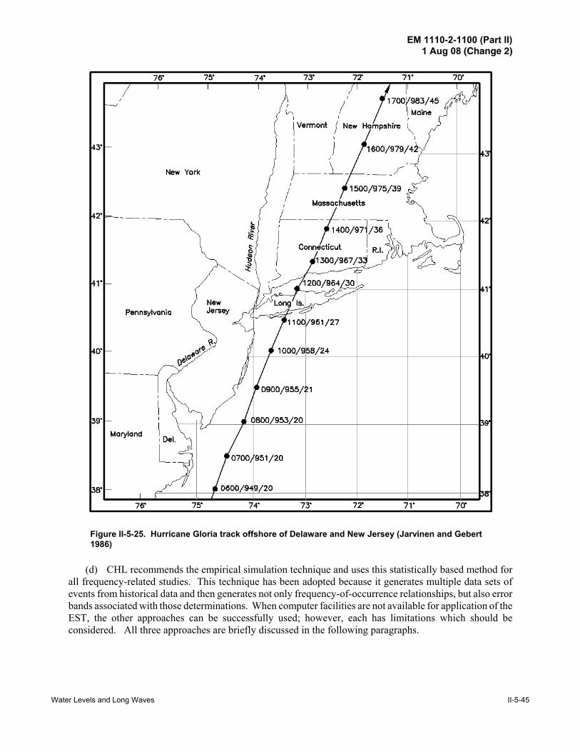
EM 1110-2-1100 (Part II)1 Aug 08 (Change 2)
Water Levels and Long Waves II-5-45
Figure II-5-25. Hurricane Gloria track offshore of Delaware and New Jersey (Jarvinen and Gebert 1986)
(d) CHL recommends the empirical simulation technique and uses this statistically based method forall frequency-related studies. This technique has been adopted because it generates multiple data sets ofevents from historical data and then generates not only frequency-of-occurrence relationships, but also errorbands associated with those determinations. When computer facilities are not available for application of theEST, the other approaches can be successfully used; however, each has limitations which should beconsidered. All three approaches are briefly discussed in the following paragraphs.

EM 1110-2-1100 (Part II)1 Aug 08 (Change 2)
II-5-46 Water Levels and Long Waves
Figure II-5-26. Example phasing of storm surge and tide (Jarvinen and Gebert 1986)
(2) Historical method.
(a) There are two basic approaches to the use of historical data for generating recurrence intervalrelationships. The first is the graphical method, the second makes use of analytical formulas to describe thebehavior of the frequency relationship.
(b) The graphical method involves construction of a cumulative probability density function (orprobability distribution function) in which the magnitude of the event is plotted against percent probabilityof exceedance.
(c) In addition to the graphical approach of developing a pdf, a variety of analytical methods exist forestimating these functions. Selection of a specific form depends on the behavior of the historical data and

EM 1110-2-1100 (Part II)1 Aug 08 (Change 2)
Water Levels and Long Waves II-5-47
the purpose of the study. One function, the Pearson Type III distribution, is presented in detail in many textson probability and statistics.
(3) Synthetic method.
(a) The synthetic method is based on the assumption that a particular event can be characterized byseveral descriptive (component) parameters, and that the probability associated with each of those parameterscan be used to determine the joint probability of the total event. For example, tropical storm events weredescribed by parameters such as radius to maximum wind, maximum wind, pressure deficit, etc. It is assumedthat the frequency of the event can be described by the frequencies associated with each parameter.
(b) The most commonly used form of the synthetic approach is the Joint Probability Method (JPM).The assumption basic to the JPM is that the probability of occurrence of a given storm event can be writtenas the product of the probabilities corresponding to each storm parameter and that the probabilities for eachparameter are independent. For example, a common assumption is that the storm can be described by fivestorm parameters. If the parameters are statistically independent, then the joint probability density functionfor the five-dimensional set is the product of the individual probability density functions, i.e.,
(II-5-24)
where fD, fR, etc., represent the pdf for the central pressure deficit D (far-field pressure pn less central pressurep0), radius to maximum R, azimuth of the storm track 2, forward speed V, and closest distance to landfall(with respect to some specified location) of the eye of the storm L. The JPM has been widely used in the pastfor storm surge analyses. Details are well-documented in USACE (1986) and the reader is referred to thatdocument for a more detailed description.
(4) Empirical simulation technique.
(a) Introduction. Few locations have an adequate historical database of storm events from which todevelop reliable stage-frequency relationships. The JPM is subject to error because it is based on simplifyingassumptions of parameter independence, and specifying the pdf of each parameter according to parametricallybased relationships. The empirical simulation technique (EST) is a statistical resampling scheme that useshistorical data to develop joint probability relationships among the various storm parameters. Theserelationships are based on data derived from actual storm events. There are no simplifying assumptionsconcerning the pdf’s; the interdependence of parameters is computed directly from the respective parameterinterdependencies contained in the historic data. In this manner, probabilities are site-specific, do not dependon fixed parametric relationships, and do not assume parameter independence. Thus, the EST is “distribution-free” and nonparametric. There are presently two approaches to applying the EST. The first approach is amulti-parameter simulation approach developed for application to tropical events. The second is a single-parameter approach developed for use in extratropical events. EST applications for tropical and extratropicalevents are discussed briefly below.
(b) EST - tropical storm application.
(1) The multi-parameter EST Program (Scheffner et al. 1999) utilizes historic data to generate a largenumber of multi-year simulations of possible future hurricane storm events for a specific location. Theapproach is based on resampling and interpolation of data contained in a database of events derived fromhistoric events. The ensemble of simulations is consistent with the statistics and correlations of past stormactivity at the site, but allows for random deviations in behavior that are likely to occur in the future.

EM 1110-2-1100 (Part II)1 Aug 08 (Change 2)
II-5-48 Water Levels and Long Waves
(2) The simulation approach is based on the selection of a set of historic “training storms” extendingover the range of storms that actually occurred at the site location. The training events are selected from thedata set of historic storms as well as from storms that could occur, such as a historic event with a slightlyshifted track. The descriptive storm parameters for each of these events (pressure deficit, radius to maximumwind, maximum wind, forward speed, angle of propagation, and tidal phase) are computed and referred toas input vectors describing each storm event.
(3) These input vectors define the multi-vector space of input parameters associated with each stormevent. These parameters are input to the PBL storm model to produce a time-varying spatial distribution ofwind and pressure fields subsequently used as input to a numerical hydrodynamic model for computing stormsurge hydrographs over the computational domain. (Examples of numerical modeling of storm surge andtidal circulation are presented in Part II-5-7.) The maximum storm surge elevation reached at specified gaugelocations is defined as the response vector of the storm at that location.
(4) Other output vectors such as maximum shoreline erosion, maximum dune recession, or maximumwave height can be described. The output vector(s) represents the environmental response to the storm. Thisresponse is defined at location X and is a direct consequence of the storm via the storm parameter valuesdefined at the point of nearest proximity of the storm eye to point X. For the case of stage-frequencyanalyses, maximum surge is assumed to occur when the eye of the storm is nearest location X.
(5) Input to the EST model is the training set database of storm input and response vector(s) for aspecific location. An example storm surge analysis for the coast of Delaware (Scheffner, Borgman, and Mark1993) identified 33 tropical events that impacted the study region during the 104-year period of 1886 through1989. Of these events, 15 were selected to be representative of the full set. All events were extracted fromthe NOAA (1981) database of historic storms. These data were used to develop input to the PBL model togenerate input data to a hydrodynamic long-wave model. Storm surge hydrographs were computed for eachof the 15 storm events. This preliminary analysis generated a set of input and response vectors for 15 stormevents for input to the EST.
(6) Each storm surge is computed independent of the local tidal phase. Each event has an equalprobability of occurring at high tide, MSL after flood, low tide, or MSL after ebb. Each of the computedsurge elevations were linearly combined with the four phases of the tide to generate an expanded training setof 60 events, which included tidal elevation.
(7) A cumulative pdf for the 60 storm events is developed based on the assumption that each of the 60events has an equal probability of occurrence, and that the number of hurricanes along the coast of Delawareis defined by the number of historical events, i.e., 33 events in 104 years. Each storm is considered a pointevent in time with each storm occurring independently. The empirical simulation technique utilizes aresampling scheme in which a random number seed from 0.0 to 1.0 is used to select a historic event from thetraining set. Each selected event is described according to its respective input vectors and the maximum surgeelevation response vector.
(8) Input vectors corresponding to the randomly selected event are used to define a new set of inputvectors, based on the initial selected storm values but weighted to reflect the value of the “nearest neighbor”parameter contained in a vector space representing parameters corresponding to all events in the 60-stormdatabase. In this manner, a new storm is defined according to a new set of parameters that is similar to thosedefining the selected event but adjusted to reflect the parameter interrelationships of the full database. Multi-vector interpolation schemes use the new event input parameters to estimate a new response parameter - thepeak storm surge at point X.

EM 1110-2-1100 (Part II)1 Aug 08 (Change 2)
Water Levels and Long Waves II-5-49
(9) The EST simulation approach is to perform N-repetitions of M-years of simulation; for example,100 simulations of a 200-year sequence of storms. Details of the EST are given in Borgman and Scheffner(1991). The number of storms simulated per year is specified according to a Poisson probability law of theform:
(II-5-25)
for n = 0,1,2,3,.... Equation II-5-25 defines the probability of having N storm events in T years. The variable8 defines the mean frequency of observed events per time period. For the example shown for the coast ofDelaware, the value of 8 was chosen to be 0.32 events per year, computed as the ratio of 33 observed eventsabove some selected threshold intensity over a 104-year period.
(10) A 10,000-element array is initialized to the above Poisson distribution. The number correspondingto 0 storms per year from Equation II-5-25 is 0.7234; thus, if a random number selection is less than or equalto 0.7234 on an interval of 0.0 to 1.0, then no hurricanes would occur during that year of simulation. If therandom number is between 0.7234 and 0.7234 + P[N=1] = 0.7234 + 0.2343 = 0.9577, one event is selected.Two events for 0.9577 + 0.0379 = 0.9956, etc. When one or more storms are indicated for a given year, theyare randomly selected from the expanded training set. In this manner, a randomly selected number of stormsper year is computed for each year to generate a 200-year simulation.
(11) Each 200-year sequence is rank ordered, a cumulative pdf computed, and a frequency-of-occurrencerelationship developed according to the approach described above. However, in the EST, tail functions(Borgman and Scheffner 1991) are used to define probabilities for events larger than the largest the 200-yearsimulation.
(12) This computation is repeated 100 times, resulting in 100 individual pdfs from which 100 stage-frequency relationships are computed. This family of curves is averaged and the standard deviationcomputed, resulting in the generation of a stage-frequency relationship containing a measure of variabilityof data spread about the mean. This variation is well-suited to the development of design criteria requiringthe quantification of the element of risk associated with the frequency predictions. A computed stage-frequency relationship for a coastal station in the Delaware study is shown in Figure II-5-27.
(c) EST - extratropical storm application.
(1) Extratropical events cannot be easily parameterized; therefore, the multi-parameter application ofthe EST is not appropriate for events such as northeasters. An alternate small-parameter application of theEST (Palermo et al. 1998) was used for this class of events. Northeasters have a much greater frequency ofoccurrence than hurricanes. For example, several northeasters impact large regions of the east coast everyyear. The existing WIS database of northeasters represents an adequate population of storms from whichfrequency-of-occurrence relationships can be computed.
(2) The extratropical EST approach is conceptually simpler than the multi-parameter version used forhurricanes because parameters such as tidal phase, wave height, and wave period are specified as inputvectors. In this approach, a database of extratropical events is assembled and respective surge elevationscomputed for each storm in the training set using numerical modeling techniques. If 20-30 years of reliablestorm surge elevation data are available for a particular location, the numerical modeling phase may not benecessary. The extratropical analogy to the tropical implementation is that there are fewer input vectors. Thedatabase of response vectors is combined with tide, rank ordered, and a pdf is computed.

EM 1110-2-1100 (Part II)1 Aug 08 (Change 2)
II-5-50 Water Levels and Long Waves
Figure II-5-27. Stage-frequency relationship - coast of Delaware
(3) The extratropical application of the EST can be used to develop recurrence relationships for anyparameter if the database of parameters is sufficiently large to define the full population of possible events.A sample application was made to a dredged disposal site located in the New York Bight, on the east coastof the United States. The goal was to determine the recurrence interval of bottom erosion resulting from the11 December 1992 extratropical storm event. An existing database of severe extratropical storms thatimpacted the Bight was available with corresponding wave conditions, maximum storm surge elevation, andtidal phase for each storm of the set. These data were used to define a database of peak sediment transportmagnitudes, computed as a function of wave height, current (computed from surge elevations), depth, andgrain size (Scheffner 1992). These data were input to the EST specifying only one input vector, the peaksediment transport magnitude (QX), to generate 1,000 repetitions of a 500-year simulation. For each500-year simulation, a transport versus frequency-of-occurrence relationship was computed. As describedabove, an average curve was computed, which included variability. Results of the analysis are shown in thetransport-frequency curve of Figure II-5-28 in which transport is given in ft3/sec/ft-width × 10-4.
(4) Historical data on storms in and around the coasts of the United States have been recorded andpublished in detail since the late 1800's. For example, NOAA publishes an atlas of tropical storms (NOAA1981) that is continuously updated to reflect recent events. The distribution of east coast tropical events overthe period of 1886-1980 is shown in Figure II-5-29, in which the tracks of the 793 Atlantic tropical cyclonesreaching at least tropical storm intensity are shown. The Wave Information Study (WIS) of CHL has hindcastdata for extratropical storms covering over 30 years.
(5) Recent advances in numerical modeling techniques make it possible to use these very large databasesof storm event track, wind, and pressure to simulate storm surges associated with each event. These sourcesprovide data used to develop storm surge versus frequency-of-occurrence relationships.

EM 1110-2-1100 (Part II)1 Aug 08 (Change 2)
Water Levels and Long Waves II-5-51
Figure II-5-28. Sediment transport magnitude-frequency relationship - December 1992northeaster
II-5-6. Seiches
a. Seiches are standing waves or oscillations of the free surface of a body of water in a closed orsemiclosed basin. These oscillations are of relatively long period, extending from minutes in harbors andbays to over 10 hr in the Great Lakes. Any external perturbation to the lake or embayment can force anoscillation. In harbors, the forcing can be the result of short waves and wave groups at the harbor entrance.Examples include 30- to 400-sec wave-forced oscillations in the Los Angeles-Long Beach harbor (Seabergh1985). Dominant long-period seiche conditions on the Great Lakes have resonant modes with periodsvarying from 2 to 12 hr. These oscillations result primarily from changes in atmospheric pressure and theresultant wind conditions and occur over the entire basin. The frequency of oscillation is a function of theforcing, together with geometry and bathymetry, of the system.
b. In areas of simple geometry, modes of oscillation can be predicted from the shape of the basin. Forexample, Figure II-5-30 shows surface profiles for various simple geometric configurations.
c. For the one-dimensional case of a closed rectangular basin with vertical walls and uniform depth(Figure II-5-30b), the natural free oscillating period Tn can be written as
(II-5-26)

EM 1110-2-1100 (Part II)1 Aug 08 (Change 2)
II-5-52 Water Levels and Long Waves
Figure II-5-29. Atlantic tropical storm tracks during the period 1886-1980
where n is the number of nodes along the axis of the basin, h is the water depth, and lB is the length of thebasin. The fundamental and maximum period corresponds to Tn for n = 1. As shown in Figure II-5-30b,nodes (locations of no vertical deflection) are located at interior points and antinodes (locations of maximumdeflection) are located on the boundaries of the basin. Longitudinal seiches oscillate from end to end, whiletransverse seiches oscillate from side to side in the basin.
d. For an open rectangular basin (Figure II-5-30c), the free oscillation period is written as follows:
(II-5-27)
e. The fundamental mode corresponds to n=0. As shown in Figure II-5-30c, the node is located on theopening with an antinode on the opposite end.

EM 1110-2-1100 (Part II)1 Aug 08 (Change 2)
Water Levels and Long Waves II-5-53
Figure II-5-30. Long wave surface profiles (Shore Protection Manual 1984)
f. Methods are available to estimate free oscillations in long narrow lakes of variable width and depth(Defant 1961); however, seiche periods and node/antinode locations are determined most accurately throughlong-wave modeling. For this class of problem, numerical solutions of the governing equations are necessary.An example is presented in Rao and Schwab (1976), in which a numerical model is used to investigate thenormal modes of oscillation in an arbitrary enclosed basin on a rotating earth. Applications are made to LakesOntario and Superior. Rao and Schwab describe two distinct types of free oscillations, gravitational modesand rotational modes. Gravitational modes result from undulations of the free surface and are independentof the rotation of the earth. Rotational modes are a function of gravity via the Coriolis parameter. Figure II-5-31 represents the first, second, and third normal modes of oscillation for Lake Ontario. The periods of thecomputed six lowest modes in Lake Ontario are 5.11, 3.11, 2.13, 1.87, 1.78, and 1.46 hr for modes 1 through6. The complexity of the nodal points and lines of phase demonstrate that idealized solutions such as thoseshown in Figure II-5-30 are often not adequate to explain natural phenomena. For applications requiringdetailed information on maximum seiche elevations and nodal distributions, numerical models such as thosedescribed in the following section are the only viable approach to developing reliable solutions.

EM 1110-2-1100 (Part II)1 Aug 08 (Change 2)
II-5-54 Water Levels and Long Waves
Figure II-5-31. First, second, and third normal modes of oscillation for LakeOntario (Rao and Schwab 1976)
II-5-7. Numerical Modeling of Long-Wave Hydrodynamics
a. Long wave modeling. Most natural flow systems are extremely complex. They have variablebathymetry and irregular shorelines and are driven by a combination of tidal, wind, and pressure forcing, aswell as temperature- and salinity-driven density gradient forcing. If a realistic approximation of flowhydrodynamics is necessary for the formulation of design criteria or testing of design alternatives (forexample), numerical long-wave hydrodynamic models should be used. Although these models are generallynot easy to apply and require mainframe computers, they provide the most accurate flow field approximation.
b. Physical models. Prior to describing example applications of numerical models, physical modelsmay provide a viable alternative to numerical approaches if the problem of concern is not wind-dominated.For example, if a physical model of a particular estuary exists, and the problem of interest is of tidal origin,

EM 1110-2-1100 (Part II)1 Aug 08 (Change 2)
Water Levels and Long Waves II-5-55
then a physical model may be cost-effective. A substantial amount of literature on physical models andmodeling is available. An extremely comprehensive source of information is Hudson et al. (1979).
c. Numerical models.
(1) Introduction.
(a) Numerical hydrodynamic models generally fall into two solution scheme categories, finite differenceand finite element. Finite difference models use a rectangular orthogonal grid, although grid transformationschemes permit the mapping of the grid to conform to curvilinear boundaries. Finite element models use avariable-size, either triangular or rectangular, unstructured computational grid. The ability to define elementsof variable size gives the finite element method an advantage over finite difference schemes for accuratelyrepresenting areas of very complex geometry. However, both modeling techniques produce accurate resultswhen applied correctly. Both models are in common use, as is demonstrated in the following two examplesof numerical model applications to specific coastal and estuarine applications. These examples are intendedto demonstrate the capability and accuracy of numerical models to reproduce natural hydrodynamic systemsand generate an appreciation for the difficulty involved with applying them to specific flow-field situations.
(b) In addition to differences in computational schemes, hydrodynamic models are also categorized as1-, 2-, and 3-dimensional. One-dimensional models provide a cross-sectional average solution to thegoverning equations. This class of solution is well-suited to pipeline or river flow problems, but notcoastal/estuarine problems. Therefore, 1-D models are not addressed in this chapter because their solutionsprovide little detailed flow-field information that cannot be computed from the formulas given in Part II-1,“Water Wave Mechanics.”
(c) Two-dimensional models are generally depth-integrated (depth-averaged); they provide a singlevelocity vector corresponding to each horizontal cell of a computational domain representing large areas ofsurface flow. Currents are defined at nodes or on cell faces, depending on the computational scheme used.Two-dimensional models are generally used in situations where the modeled system is well-mixed, i.e.,currents are approximately uniform throughout the water column. These models are appropriate for studiesin which changes in surface elevation are the primary concern. Typical examples include storm surge or lakeseiche studies.
(d) An additional class of two-dimensional models is the laterally averaged model. In this case, insteadof depth-averaged governing equations, a width-averaged set of equations is defined. In this form of solution,currents are defined at multiple locations through the water column; however, no horizontal distributioninformation is given. Laterally averaged models are generally used in conjunction with river flow, reservoiroperation, and/or salinity intrusion applications and these models are not described in this manual.
(e) Three-dimensional applications are used when the vertical structure of currents is not uniform andthe vertical distribution of currents is an important aspect of the study. Example applications include areasexhibiting flow reversal situations where surface currents and bottom currents flow in opposite directions.Included in this class of problems are cases in which vertical temperature and salinity gradients create density-driven flows. Although these non-tidal flows can be small in comparison to the tidal ebb and flood currents,they can contribute to residual circulation patterns that may affect the transport and dispersion of certain waterquality parameters such as dissolved oxygen. An additional example may include channel-deepening effectson salinity intrusion.

EM 1110-2-1100 (Part II)1 Aug 08 (Change 2)
II-5-56 Water Levels and Long Waves
(f) Before presenting example applications of models, it is stressed that all models are not equal withrespect to computational speed and accuracy. Depending on how the governing equations are written andsolved and how and what boundary conditions are defined and used to drive the models, any two finite-element or finite-difference models can produce different results. Therefore, for some applications, onemodel may produce accurate results while another formulation will be unstable and produce totally unrealisticsimulations. For this reason, any application of a numerical model should begin with a calibration andverification procedure in which the model is run to reproduce the hydrodynamic flow field corresponding toa specific time period during which prototype data (i.e., surface elevations and currents) have been collected.Additional data comparisons may include hydrodynamically driven parameters such as temperatures andsalinities.
(g) In the calibration phase, model parameters such as the friction factor distribution or depth resolutionare adjusted to optimize the comparison of model-generated data to measured prototype data. Comparisonsare generally made to surface elevations and velocities, but may include reproduction of temperature andsalinity. In the verification procedure, the model is used to simulate an alternate time period containingadditional prototype data. Model coefficients are not adjusted in the verification phase. An acceptablecalibration and verification demonstrates that the model is capable of simulating the total flow regime overthe entire computational domain. This ability is basic and necessary to the use of numerical models toquantify the flow-field response to proposed or existing changes in flow-field boundaries.
(h) If data are available or can be collected, the calibration and verification procedures represent aminimum criterion required of a model before it can be applied to any specific problem. If these two stepsare not performed in a satisfactory manner, model results can only be considered qualitative. Situations doexist where prototype data are not available and cannot be obtained within the time and cost limits of thebudget. In these cases, models can be used to generate qualitative trends; however, unverified model resultsshould not be the basis for quantitative decision making unless some data are available, even at a minimumlevel, to demonstrate that the model is producing realistic results. This aspect of modeling may be vital toa particular project because decisions based on unverified model results can be legally challenged and shownto be invalid.
(2) Example - tidal circulation modeling.
(a) The New York Bight project (Scheffner et al. 1993) is an excellent example of tidal circulationmodeling. The goal of the study was to develop a hydrodynamic simulation tool that could be used to addressquestions concerning how certain modifications to the New York Bight may affect the local or globalhydrodynamics of the system and how the computed flow fields affected the transport of certain water qualityparameters. The model was therefore required to be capable of simulating the flow-field hydrodynamics,temperature, and salinity distribution over a large computational domain.
(b) The model selected for this study was the CH3D (Curvilinear Hydrodynamics in Three (3)Dimensions) (Johnson et al. 1991) model, a three-dimensional, finite difference formulation model withboundary-fitted coordinates. The modeled area represents the region extending offshore from Cape May, NJ,and Nantucket Shoals to beyond the continental shelf, including Long Island Sound, the Hudson andEast Rivers, and New York Harbor. Depths vary from less than 10 m to more than 2,000 m. Thegeographical boundaries are shown in Figure II-5-32a. The computational grid used to represent this areaof interest is shown in Figure II-5-32b. The grid contains 76 cells in the alongshore direction and 45 cellsin the cross-shore direction. There are 2,641 active computational cells in the horizontal and 10 in thevertical.
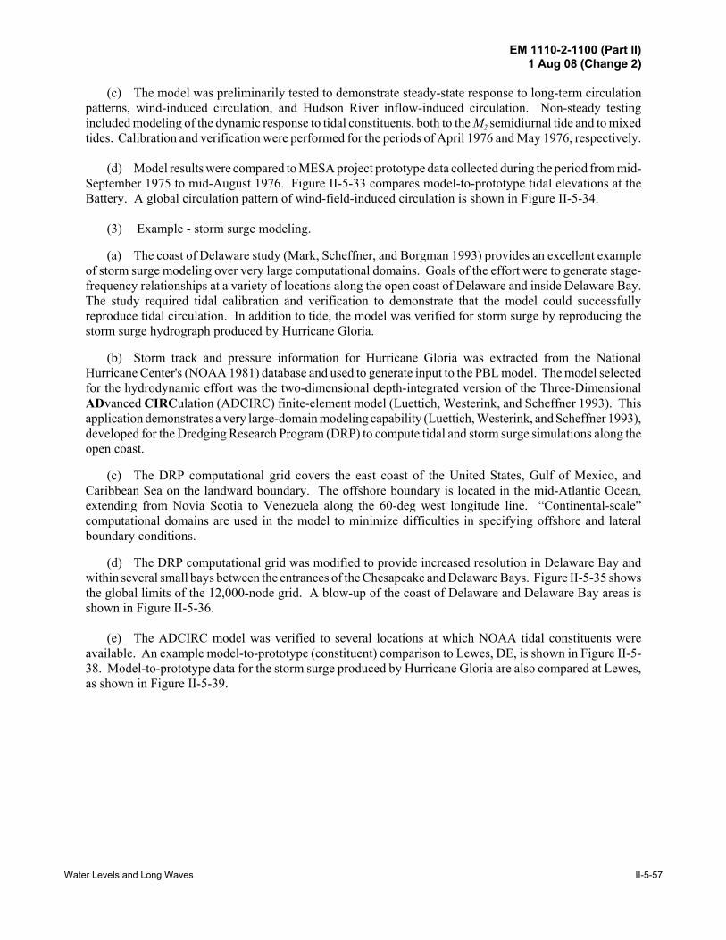
EM 1110-2-1100 (Part II)1 Aug 08 (Change 2)
Water Levels and Long Waves II-5-57
(c) The model was preliminarily tested to demonstrate steady-state response to long-term circulationpatterns, wind-induced circulation, and Hudson River inflow-induced circulation. Non-steady testingincluded modeling of the dynamic response to tidal constituents, both to the M2 semidiurnal tide and to mixedtides. Calibration and verification were performed for the periods of April 1976 and May 1976, respectively.
(d) Model results were compared to MESA project prototype data collected during the period from mid-September 1975 to mid-August 1976. Figure II-5-33 compares model-to-prototype tidal elevations at theBattery. A global circulation pattern of wind-field-induced circulation is shown in Figure II-5-34.
(3) Example - storm surge modeling.
(a) The coast of Delaware study (Mark, Scheffner, and Borgman 1993) provides an excellent exampleof storm surge modeling over very large computational domains. Goals of the effort were to generate stage-frequency relationships at a variety of locations along the open coast of Delaware and inside Delaware Bay.The study required tidal calibration and verification to demonstrate that the model could successfullyreproduce tidal circulation. In addition to tide, the model was verified for storm surge by reproducing thestorm surge hydrograph produced by Hurricane Gloria.
(b) Storm track and pressure information for Hurricane Gloria was extracted from the NationalHurricane Center's (NOAA 1981) database and used to generate input to the PBL model. The model selectedfor the hydrodynamic effort was the two-dimensional depth-integrated version of the Three-DimensionalADvanced CIRCulation (ADCIRC) finite-element model (Luettich, Westerink, and Scheffner 1993). Thisapplication demonstrates a very large-domain modeling capability (Luettich, Westerink, and Scheffner 1993),developed for the Dredging Research Program (DRP) to compute tidal and storm surge simulations along theopen coast.
(c) The DRP computational grid covers the east coast of the United States, Gulf of Mexico, andCaribbean Sea on the landward boundary. The offshore boundary is located in the mid-Atlantic Ocean,extending from Novia Scotia to Venezuela along the 60-deg west longitude line. “Continental-scale”computational domains are used in the model to minimize difficulties in specifying offshore and lateralboundary conditions.
(d) The DRP computational grid was modified to provide increased resolution in Delaware Bay andwithin several small bays between the entrances of the Chesapeake and Delaware Bays. Figure II-5-35 showsthe global limits of the 12,000-node grid. A blow-up of the coast of Delaware and Delaware Bay areas isshown in Figure II-5-36.
(e) The ADCIRC model was verified to several locations at which NOAA tidal constituents wereavailable. An example model-to-prototype (constituent) comparison to Lewes, DE, is shown in Figure II-5-38. Model-to-prototype data for the storm surge produced by Hurricane Gloria are also compared at Lewes,as shown in Figure II-5-39.

EM 1110-2-1100 (Part II)1 Aug 08 (Change 2)
II-5-58 Water Levels and Long Waves
Figure II-5-32. Computational grid for the New York Bight

EM 1110-2-1100 (Part II)1 Aug 08 (Change 2)
Water Levels and Long Waves II-5-59
Figu
re II
-5-3
3.
Mod
el a
nd p
roto
type
tida
l ele
vatio
n co
mpa
rison
at t
he B
atte
ry
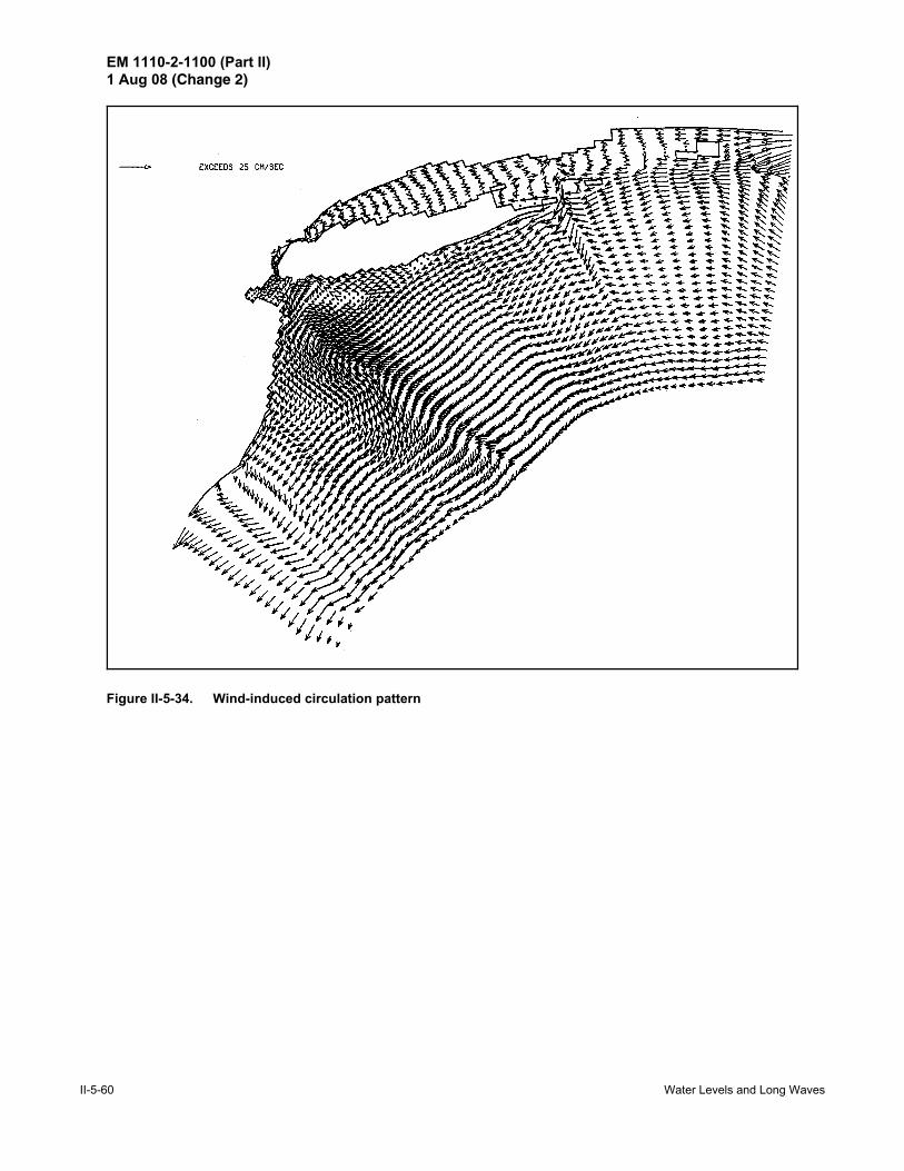
EM 1110-2-1100 (Part II)1 Aug 08 (Change 2)
II-5-60 Water Levels and Long Waves
Figure II-5-34. Wind-induced circulation pattern

EM 1110-2-1100 (Part II)1 Aug 08 (Change 2)
Water Levels and Long Waves II-5-61
Figure II-5-35. Global limits of ADCIRC computational grid

EM 1110-2-1100 (Part II)1 Aug 08 (Change 2)
II-5-62 Water Levels and Long Waves
Figure II-5-36. Blow-up of ADCIRC grid along Delaware coast

EM 1110-2-1100 (Part II)1 Aug 08 (Change 2)
Water Levels and Long Waves II-5-63
Figure II-5-37. Model-to-prototype tidal comparison at Lewes, DE

EM 1110-2-1100 (Part II)1 Aug 08 (Change 2)
II-5-64 Water Levels and Long Waves
Figure II-5-38. Model-to-prototype surge comparison at Lewes, DE
II-5-8. References
EM 1110-2-1415Hydrologic Frequency Analysis
Borgman and Resio 1982Borgman, L. E., and Resio, D. T. 1982. “Extremal Statistics in Wave Climatology,” Topics in OceanPhysics, A. Osborne and P. M. Rizzoli, ed., Italian Physical Society, Bologna, Italy, pp 439-471.
Borgman and Scheffner 1991 Borgman, L. E., and Scheffner, N. W. 1991. “The Simulation of Time Sequences of Wave Height, Period,and Direction,” Technical Report TR-DRP-91-2, U.S. Army Engineer Waterways Experiment Station,Vicksburg, MS.
Camfield 1980Camfield, F. E. 1980. “Tsunami Engineering,” Special Report No. 6, U.S. Army Engineer WaterwaysExperiment Station, Vicksburg, MS.

EM 1110-2-1100 (Part II)1 Aug 08 (Change 2)
Water Levels and Long Waves II-5-65
CCCMSL 1987Committee on Engineering Implications of Changes in Relative Mean Sea Level. 1987. “Responding toChanges in Sea Level Engineering Implications,” Marine Board, Commission on Engineering and TechnicalSystems, National Research Council. National Academy Press, Washington, DC, 148 p.
Cialone et al. 1991Cialone, M. A., Mark, D. J., Chou, L. W., Leenknecht, D. A., Davis, J. A., Lillycrop. L. S., Jensen, R. E.,Thompson, E. F., Gravens, M. B., Rosati, J. D., Wise, R. A., Kraus, N. C., and Larson, P. M. 1991. “CoastalModeling System (CMS) User’s Manual,” Instruction Report CERC-91-1, U.S. Army Engineer WaterwaysExperiment Station, Vicksburg, MS.
Coordinating Committee on Great Lakes Basin Hydraulic and Hydrologic Data 1992Coordinating Committee on Great Lakes Basin Hydraulic and Hydrologic Data. 1992. Brochure on theInternational Great Lakes Datum 1985, U.S. Government Printing Office, 1992-644-640.
Defant 1961Defant, A. 1961. Physical Oceanography, Vol II, Pergamon Press, New York.
Dronkers 1964Dronkers, J. J. 1964. “Tidal Computations in Rivers and Coastal Waters,” North-Holland PublishingCompany - Amsterdam, John Wiley & Sons, Inc., New York.
Graham and Nunn 1959Graham, H. E., and Nunn, D. E. 1959. “Meteorological Considerations Pertinent to Standard ProjectHurricane, Atlantic and Gulf Coasts of the United States,” National Hurricane Research Project, Report No.33, Department of Commerce, Washington, DC.
Gravens, Scheffner, and Hubertz 1989Gravens, M. B., Scheffner, N. W., and Hubertz, J. M. 1989. “Coastal Processes from Asbury Park toManasquan, New Jersey,” Miscellaneous Paper CERC-89-11, U.S. Army Engineer Waterways ExperimentStation, Vicksburg, MS. Gumbel 1954Gumbel, E. J. 1954. “Statistical Theory of Extreme Value and Some Practical Application,” National Bureauof Standards Applied Math. Series 33, U.S. Gov. Publication, Washington, DC.
Harris 1981Harris, D. L. 1981. “Tides and Tidal Datums in the United States,” Special Report No. 7, U.S. Army Corpsof Engineers, Fort Belvoir, VA., U.S. Government Printing Office (GPO Stock No. 008-022-00161-1).
Ho et al. 1987Ho, F. P., Su, J. C., Hanevich, K. L., Smith, R. J., and Richards, F. P. 1987. “Hurricane Climatology for theAtlantic and Gulf Coasts of the United States,” NOAA Technical Report NWS 38.
Hubertz et al. 1993Hubertz, J. M., Brooks, R. M., Brandon, W. A., and Tracy, B. A. 1993. “Hindcast Wave Information for theU.S. Atlantic Coast,” WIS Report 30, U.S. Army Engineer Waterways Experiment Station, Vicksburg, MS.

EM 1110-2-1100 (Part II)1 Aug 08 (Change 2)
II-5-66 Water Levels and Long Waves
Hudson et al. 1979Hudson, R. Y., Herrmann, F. A., Sager, R. A., Whalin, R. W., Keulegan, G. H., Chatham, C. E., and Hales,L. Z. 1979. “Coastal Hydraulic Models,” Special Report No. 5, Coastal Engineering Research Center,U.S. Army Engineer Waterways Experiment Station, Vicksburg, MS.
Ippen 1966Ippen, A. T. 1966. Estuary and Coastline Hydrodynamics. McGraw-Hill Book Company, Inc., New York.
Jarvinen and Gebert 1986Jarvinen, B., and Gebert, J. 1986. “Comparison of Observed Versus Slosh Model Computed Storm SurgeHydrographs along the Delaware and New Jersey Shorelines for Hurricane Gloria, September 1985,” NOAATechnical Memorandum NWS NHC 32, National Hurricane Center, Coral Gables, FL.
Johnson et al. 1991Johnson, B. H., Heath, R. E., Hsieh, H. H., Kim, K. W., and Butler, H. L. 1991. “Development andVerification of a Three-Dimensional Numerical Hydrodynamic, Salinity, and Temperature Model ofChesapeake Bay; Volume I, Main Text and Appendix D,” Technical Report HL-91-7, U.S. Army EngineerWaterways Experiment Station, Vicksburg, MS.
Leenknecht, Szuwalski, and Sherlock 1992Leenknecht, D. A., Szuwalski, A., and Sherlock, A. R. 1992. “Automated Coastal Engineering System UserGuide and Technical Reference, Version 1.07,” U.S. Army Engineer Waterways Experiment Station,Vicksburg, MS.
Luettich, Westerink, and Scheffner 1993 Luettich, R. A., Westerink, J. J., and Scheffner, N. W. 1993. “ADCIRC: An Advanced Three-DimensionalCirculation Model for Shelves, Coasts and Estuaries; Report 1: Theory and Methodology of ADCIRC-2DDIand ADCIRC-3DL,” Technical Report DRP-92-6, U.S. Army Engineer Waterways Experiment Station,Vicksburg, MS.
Mark and Scheffner 1997Mark, D. J., and Scheffner, N. W. 1997. “Coast of Delaware Hurricane Stage-Frequency Analysis,”Miscellaneous Paper CHL-97-1, U.S. Army Engineer Waterways Experiment Station, Vicksburg, MS.
Milne-Thompson 1960Milne-Thompson, L. M. 1960. Theoretical Hydrodynamics. The MacMillan Company, New York.
Morang, Mossa, and Larson 1993Morang, A., Mossa, J., and Larson, R. J. 1993. “Technologies for Assessing the Geologic and GeomorphicHistory of Coasts,” Technical Report CERC-93-5, U.S. Army Engineer Waterways Experiment Station,Vicksburg, MS.
National Oceanic and Atmospheric Administration 1977National Oceanic and Atmospheric Administration. 1977. “NOAA Federal Coordinator for MeteorologicalServices and Supporting Research, 1977: National Hurricane Operations Plan, MO 77-2.”
National Oceanic and Atmospheric Administration 1981National Oceanic and Atmospheric Administration. 1981. “Tropical Cyclones of the North Atlantic Ocean1971-1980,” U.S. Government Printing Office, Washington, DC.
EM 1110-2-1100 (Part II)1 Aug 08 (Change 2)
Water Levels and Long Waves II-5-67
National Oceanic and Atmospheric Administration 1984National Oceanic and Atmospheric Administration. 1984. “Tide Tables 1984 High and Low WaterPredictions, East Coast of North and South America, Including Greenland,” National Ocean Service,Rockville, MD.
Palermo et al. 1998Palermo, M. R., Clausner, J. E., Rollings, M. P., Williams, G. L., Myers, T. E., Fredette, T. J., and Randall,R. E. 1998. “Guidance for Subaqueous Dredged Material Capping,” Technical Report DOER-1, U.S. ArmyEngineer Waterways Experiment Station, Vicksburg, MS.
Rao and Schwab 1976 Rao, D. B., and Schwab, D. J. 1976. “Two Dimensional Normal Modes in Arbitrary Enclosed Basins on aRotating Earth: Application to Lakes Ontario and Superior,” Philosophical Transactions of the Royal Societyof London, Vol 281, pp 63-96.
Rappleye 1932Rappleye, H. S. 1932. “The 1929 Adjustment of the Level Net,” The Military Engineer, Vol 24, No. 138,pp 576-578.
Saffir 1977Saffir, H. S. 1977. “Design and Construction Requirements for Hurricane Resistant Construction,” AmericanSociety of Civil Engineers, Reprint Number 2830, New York.
Scheffner 1992Scheffner, N. W. 1992. “A Numerical Simulation Approach to Estimating Disposal Site Stability,” 1992National Conference on Hydraulic Engineering, Baltimore, MD.
Scheffner, Borgman, and Mark 1993Scheffner, N. W., Borgman, L. E., and Mark, D.J. 1993. “Applications of Large Domain HydrodynamicModels to Generate Frequency-of-Occurrence Relationships,” 3rd International Conference on Estuarine andCoastal Modeling, Chicago, IL.
Scheffner et al. 1994Scheffner, N. W., Vemulakonda, S. R., Kim, K. W., Mark, D. J., and Butler, H. L. 1994. “New York BightStudy; Report 1: Hydrodynamic Modeling,” Technical Report CERC-94-4, U.S. Army Engineer WaterwaysExperiment Station, Vicksburg, MS.
Scheffner et al. 1999Scheffner, N. W., Clausner, J. E., Militello, A., Borgman, L. E., Edge, B. L., and Grace, P. E. 1999. Use andApplication of the Empirical Simulation Technique: Users Guide, Technical Report CHL-99-21, U.S. ArmyEngineer Waterways Experiment Station, Vicksburg, MS.
Seabergh 1985Seabergh, W. C. 1985. “Los Angeles and Long Beach Harbors Model Study, Deep-Draft Dry Bulk ExportTerminal, Alternative No. 6: Resonant Response and Tidal Circulation Studies,” Miscellaneous Paper CERC-85-8, U.S. Army Engineer Waterways Experiment Station, Vicksburg, MS.
Sears and Zemansky 1963Sears, F. W., and Zemansky, M. W. 1963. University Physics. Addison-Wesley Publishing Company, Inc.,Reading, MA.

EM 1110-2-1100 (Part II)1 Aug 08 (Change 2)
II-5-68 Water Levels and Long Waves
Shalowitz 1964Shalowitz, A. L. 1964. “Shore and Sea Boundaries,” Vol 2, Publication 10-1, U.S. Coast and GeodeticSurvey, Washington, DC.
Shore Protection Manual 1984Shore Protection Manual. 1984. 4th ed., 2 Vol, U. S. Army Engineer Waterways Experiment Station,U.S. Government Printing Office, Washington, DC.
Scheffner et al. 1999Scheffner, N. W., Clausner, J. E., Militello, A., Borgman, L. E., Edge, B. L., and Grace, P. E. 1999. Use andApplication of the Empirical Simulation Technique: Users Guide, Technical Report CHL-99-21, U.S. ArmyEngineer Waterways Experiment Station, Vicksburg, MS.
Schureman 1924Schureman, P. 1924. “Manual of Harmonic Analysis and Prediction of Tides,” Special Publication No. 98,U.S. Department of Commerce, Coast and Geodetic Survey, U.S. Government Printing Office, Washington,DC.

EM 1110-2-1100 (Part II)1 Aug 08 (Change 2)
Water Levels and Long Waves II-5-69
II-5-9. Definitions of Symbols
«P Vector gradient operator (Equation II-5-11)
" Inflow angle (tropical storm parameter) [deg]
. Tidal phase lag [deg]
2 Angle of storm propagation (tropical storm parameter) [deg]
6n Epoch of constituent n, i.e., phase shift from tide-producing force to high tide fromt0 [deg]
6! Modified form of the epoch that automatically accounts for the longitude and timemeridian corrections (Equation II-5-20) [deg]
8 Mean frequency of observed events per time period used in the Poisson probabilitylaw (Equation II-5-25)
F Angular frequency (= 2B/T) [time-1]
a Wave amplitude [length]
an Speed of tide constituent n [degrees/time]
bPX Attractive force of the moon and sun at any point X (Equation II-5-10)
C Wave celerity [length/time]
f Universal constant (= 6.67 × 10⁻⁸ cm3/ gm sec2)
Fg Gravitational force (Equation II-5-7) [force-length/time2]
fn Factor for adjusting mean tidal amplitude Hn values for specific times
g Gravitational acceleration [length/time2]
h Water depth [length]
H(t) Height of the tide at any time t (Equation II-5-16) [length]
H0 Mean water level above some defined datum [length]
Hn Mean amplitude of tidal constituent n [length]
k Wave number (= 2B/L = 2B/CT) [length-1]
L Wave length [length]
lB Length of a basin [length]
M Mass of the moon
n Number of nodes along the axis of a basin
N Number of storm events used in the Poisson probability law (Equation II-5-25)
-O The subscript 0 denotes deepwater conditions

EM 1110-2-1100 (Part II)1 Aug 08 (Change 2)
II-5-70 Water Levels and Long Waves
p0 Central pressure of the eye of the storm (tropical storm parameter) [force/length2]
PM , PS Harmonic polynomial expansion terms that collectively describe the relativepositions of the earth, moon, and sun (Equations II-5-14 and II-5-15)
pn Peripheral or far-field pressure (tropical storm parameter) [force/length2]
P[N=n] Poisson probability law (Equation II-5-25)
r Distance between the centers of mass of two bodies (Equation II-5-7) [length]
R Radius to maximum wind (tropical storm parameter) [length]
R Tide classification parameter (Equation II-5-22) [dimensionless]
rm Distance from the center of the earth to the center of the moon [length]
rmx Distance of a point located on the surface of the earth to the center of the moon[length]
rs Distance from the center of the earth to the center of the sun [length]
rsx Distance of a point located on the surface of the earth to the center of the sun[length]
S Local time meridian (Equation II-5-17)
S Mass of the sun
t Time measured from some initial epoch or time
T Number of years used in the Poisson probability law (Equation II-5-25)
T Wave period [time]
Tn Natural free oscillating period of a basin (Equation II-5-26) [time]
u Fluid velocity (water particle velocity) in the x-direction [length/time]
V Maximum wind (tropical storm parameter) [length/time]
Vf Forward speed of the eye of the storm (tropical storm parameter) [length/time]
VM , VS Attractive force potentials per unit mass for the moon and sun (Equation II-5-9)
w Fluid velocity (water particle velocity) in the z-direction [length/time]
z Water depth below the SWL [length]
EM 1110-2-1100 (Part II)1 Aug 08 (Change 2)
Water Levels and Long Waves II-5-71
II-5-10. Acknowledgments
Author of Chapter II-5, “Water Levels and Long Waves:”
Norman W. Scheffner, Ph.D., Coastal and Hydraulics Laboratory, Engineer Research and DevelopmentCenter (CHL), Vicksburg, Mississippi (retired).
Reviewers:
Zeki Demirbilek, Ph.D., CHL.Lee E. Harris, Ph.D., Department of Marine and Environmental Systems, Florida Institute of Technology,
Melbourne, Florida.Edward F. Thompson, Ph.D., CHL.


![17.2 Sound Waves: In Halliday and Resnick: Longitudinal waves are sound waves! Chapter 17: [Sound] Waves-(II) Sound waves propagate in gases. Can they.](https://static.fdocuments.net/doc/165x107/56649eb25503460f94bb9375/172-sound-waves-in-halliday-and-resnick-longitudinal-waves-are-sound-waves.jpg)
