WATER CONSERVATION FROM ROOFTOP

RAINWATER HARVESTING IN

AUSTIN, TEXAS

by

Darin Daniel Rice, B.S. Geography

A directed research report submitted to the Geography Department of Texas State University in partial fulfillment

of the requirements for the degree of Master of Applied Geography

with a specialization in Geographic Information Science May 2021

Committee Members:

Advisor: Timothy T. Loftus, Ph.D.

Nathan Allan Currit, Ph.D.

v

ACKNOWLEDGEMENTS

Without great teachers and professors this work would be incomprehensible. I

acknowledge all my previous educators for their contribution to this accomplishment.

They sowed the seeds for my enlightenment and passion for all things water. Especially

significant to the completion of this research are my advisor, Timothy T. Loftus, Ph.D.,

and committee member, Nathan Allan Currit, Ph.D. Their willingness to support this

research, provide indispensable feedback, and their valuable time are much appreciated.

Without great bosses this work would be unrealistic. I acknowledge all the bosses

I have had the pleasure to work under through my graduate school endeavors. My most

ardently supportive boss, John Sutton, has provided the time and guidance necessary to

focus on this research.

Without great friends, family, and coworkers this work would be constrained by

my thoughts alone. I acknowledge all these great people as they have allowed me to have

no other topic of discussion but water. Above all, I thank my wonderful partner, Nicole,

who has shouldered a significant load of family affairs and provided vital encouragement

over these many years.

vi

Table of Contents ACKNOWLEDGEMENTS ................................................................................................ v LIST OF TABLES ........................................................................................................... viii LIST OF FIGURES ........................................................................................................... ix ABSTRACT ........................................................................................................................ x 1. Introduction ................................................................................................................. 1 2. Literature Review ........................................................................................................ 3

2.1 Rainwater harvesting: a background .................................................................... 3 2.2 Rainwater harvesting: a calculation ..................................................................... 7 2.3 Outdoor water demand ......................................................................................... 9 2.4 Classifying residential landscapes using remote sensing techniques ................. 12

3. Data Acquisition and Application ............................................................................. 14 3.1 Water system boundary ...................................................................................... 15 3.2 Land parcels ....................................................................................................... 16 3.3 Building footprints ............................................................................................. 19 3.4 Precipitation and evapotranspiration .................................................................. 21 3.5 Runoff and plant water use coefficients ............................................................. 24 3.6 Water use ............................................................................................................ 25

4. Method ....................................................................................................................... 29 4.1 Supervised classification .................................................................................... 30 4.2 Reclassification and landscaped area square footage ......................................... 35 4.3 Outdoor demand ................................................................................................. 38 4.4 Collected supply ................................................................................................. 39

5. Results and Discussion .............................................................................................. 40 5.1 Outdoor demand ................................................................................................. 40 5.2 Collected supply ................................................................................................. 41 5.3 How much water can be collected and conserved? ............................................ 41

6. Conclusion ................................................................................................................. 51 References ......................................................................................................................... 54 APPENDIX A. City of Austin, Annual Water Use Survey (2019) .................................. 57 APPENDIX B. Six Study Sample Area Classified Images .............................................. 61

vii

APPENDIX C. Six Study Sample Area Classified Image Confusion Matrices ............... 68 APPENDIX D. Collective and Individual Single-Family Residential Rainwater Harvesting Calculations (Austin) ...................................................................................... 71

viii

LIST OF TABLES

Table Page Table 1. Average monthly rainfall totals for Camp Mabry station in central Austin, Texas. ........................................................................................................................... 21 Table 2. Average monthly evapotranspiration for LCRA (Redbud) station in Austin, Texas. .................................................................................................................. 22 Table 3. West-southwest Pflugerville tile sample area confusion matrix. ..................... 34 Table 4. Comparison of collective single-family residential outdoor irrigation demand. 43 Table 5. Comparison of individual single-family residential outdoor irrigation demand. 44 Table 6. Outdoor irrigation demand conserved by 12,500 gallons of storage before and after landscape conversion on an average Austin single-family residential property. ..... 48 Table 7. Outdoor irrigation demand conserved by 5,000 gallons of storage before and after landscape conversion on an average Austin single-family residential property. ..... 49 Table 8. Outdoor irrigation demand conserved by 1,000 gallons of storage before and after landscape conversion on an average Austin single-family residential property. ..... 50

ix

LIST OF FIGURES Figure Page Figure 1. Austin water system boundary. Inset in Texas for location. .......................... 16 Figure 2. Single-family parcels of 0.5 acres or less example from northwest Montopolis orthoimagery tile. .................................................................................................. 18 Figure 3. Single-family building footprints on parcels of 0.5 acres or less in northwest Montopolis orthoimagery tile. ................................................................................ 20 Figure 4. Stacked line chart of average monthly rainfall and average monthly evapotranspiration for weather stations in Austin, Texas. .......................................... 23 Figure 5. Stacked line chart of average monthly plant water needs and average monthly rainfall in Austin, Texas. ........................................................................................ 24 Figure 6. Kernel density of building footprint points per square mile classified into ten equal-interval classes. ............................................................................................ 28 Figure 7. TNRIS orthoimagery tile locations. Each polygon is the name of the original orthoimagery tile set: (a) west southwest Pflugerville, (b) east northwest Austin, (c) east southeast Austin, (d) northeast Oak Hill, (e) northwest Oak Hill, and (f) northwest Montopolis. .......................................................................................................... 29 Figure 8. Orthographic imagery of extracted residential areas used for supervised classification in six orthoimagery areas within Austin Water boundary: (a) west southwest Pflugerville, (b) east northwest Austin, (c) east southeast Austin, (d) northeast Oak Hill, (e) northwest Oak Hill, and (f) northwest Montopolis. ................................ 31 Figure 9. Orthographic imagery of extracted residential areas classified in six orthoimagery areas within Austin Water boundary: (a) west southwest Pflugerville, (b) east northwest Austin, (c) east southeast Austin, (d) northeast Oak Hill, (e) northwest Oak Hill, and (f) northwest Montopolis. ......................................................................... 33 Figure 10. Progression of a sample parcel from orthoimagery to classified to reclassified. ........................................................................................................................... 37 Figure 11. Comparison of storage tank diameters on average sized study area parcel. ... 46

x

ABSTRACT

Rooftop rainwater harvesting may provide an alternate supply of water for many

household uses. There is a significant potential for supply from rooftop rainwater

harvesting systems to offset the use of utility potable water used for outdoor irrigation

demand from landscaped areas in Austin, Texas. To calculate the potential savings of

these systems a supply and demand are needed. Monthly average rainfall totals, the area

of building footprints of over two hundred thousand single-family residential parcels, and

a roof material runoff coefficient were used to calculate the potential volume collected

from rooftop rainwater harvesting. Monthly average evapotranspiration totals, the area of

landscaped areas of over two hundred thousand single-family residential parcels, and a

plant water use coefficient were used to calculate the potential volume conserved from

rooftop rainwater harvesting. Object-based, supervised land-use classification was

performed on sample areas to obtain the average landscaped area in Austin. The results of

this study may help local, regional, and state water planners quantify the potential volume

of water collected and conserved from the implementation of rooftop rainwater

harvesting systems.

1

WATER CONSERVATION FROM ROOFTOP RAINWATER HARVESTING IN

AUSTIN, TEXAS

1. Introduction

The world population is growing rapidly. The United Nations’ World

Urbanization Prospects: The 2018 Revision states the future world population growth

will be made up primarily of city dwellers (United Nations 2019). This is evident in the

capitol of Texas, Austin, a city located in the central part of the state. In July 2019, the

city was designated the eleventh most populous city in the United States of America

(USA) (United States Census Bureau 2020). The state projects by 2070 over 1.7 million

people will reside in the Austin area, an increase from over nine hundred and seventy-six

thousand in 2020 (Texas Water Development Board 2017).

As the city grows water planning becomes an important component to ensuring

the water needs of the population are met. In Texas, state water planning is published in a

report, the State Water Plan, every five years. The plan projects water supply and demand

in the state assuming drought of record conditions. These conditions represent when

supplies are their lowest and demands are their highest referencing a period in Texas

known as the worst drought in state history, the drought of record. State water plans and

the process of evaluating projected demands, current supplies, potential shortages, and

feasible water management strategies are legislatively mandated. A state agency, the

Texas Water Development Board (TWDB), compiles regional water planning reports and

other data to produce projections over a fifty year period by regional water planning area,

river basin, county, and water user group (TWDB 2017).

Water user groups are divided into six categories: irrigation, municipal,

2

manufacturing, steam-electric power, livestock, and mining. The City of Austin

represents one of the many municipal water user groups in the state. The Austin water

user group is also known as the city of Austin’s water utility, Austin Water. Austin

Water, heretofore referred to as Austin, provides water for many uses including

residential uses in Hays, Travis, and Williamson counties. In the most recent state water

plan published in 2017, Austin supplies are projected to decrease by over 17 percent and

demand is projected to increase by over 75 percent by 2070. By 2050, Austin is projected

to have a potential water shortage due to demand outpacing supply. To meet water

demands, due to population growth, water management strategies will be needed (TWDB

2017).

Water management strategies must identify a new source of water to be accepted

in the water planning process (TWDB 2010). The strategies for Austin include, but are

not limited to, aquifer storage and recovery, direct reuse, conservation, lake and dam

improvements, drought management, and rainwater harvesting (TWDB 2017). Austin

plans to supply 16,564 acre feet per year by 2070 from rainwater harvesting alone, an

increase of over 16,000 acre feet per year from 2020 projections. For comparison, aquifer

storage and recovery, conservation, and drought management are projected to provide

50,000, 36,899, and 28,937 acre feet per year, respectively, by 2070 (Lower Colorado

Regional Water Planning Group 2016).

Though not as large a volume of projected supply as these other strategies, the

rainwater harvesting strategy only represents supplemental non-potable water use from

rainwater catchment by customers in Austin. The cost to meet the rainwater harvesting

strategy is projected over $690 million by 2070, representing over 40 percent of the total

3

capital cost of all recommended projects for Austin in the 2017 State Water Plan. The

$690 million represents the cost incurred by Austin in the form of rebates to over one

hundred and thirty-eight thousand water customers for implementation of rainwater

harvesting systems and does not include the full cost of installation, operation, and

maintenance incurred by the customers. These rebates help alleviate the customer cost

burden while decreasing the use of surface water and groundwater, and the treatment cost

associated (Lower Colorado Regional Water Planning Group 2016).

In this study, the potential volume of water collected and conserved from single-

family residential rooftop rainwater harvesting in Austin will be evaluated. Just like state

and regional water planning, calculating rainwater harvesting potential requires supply

and demand. The volume collected from rainwater harvesting systems represents the

supply and the water needs of plants in the landscaped area represent the demand. A cost

to implement is also necessary however this study seeks to answer the rainwater

harvesting potential without regard to cost. The goal of this study is, therefore, to identify

whether implementing rooftop rainwater harvesting systems on all single-family

residential properties can collect enough supply to conserve the large volume of valuable

potable water currently used to irrigate these landscaped areas.

2. Literature Review

2.1 Rainwater harvesting: a background

The use of captured rainwater has been practiced for thousands of years. Dating

back 10,000 years, early hunter-gatherers in the Chihuahuan Desert used water naturally

collected in rock formations now known as the Hueco Tanks located in an area east of

4

current day El Paso, Texas (Texas Parks and Wildlife Department 2021). Over 4,000

years ago the concept of rainwater harvesting is documented from archeological evidence

of cisterns, or storage tanks, in Israel (TWDB 2005). Present-day rainwater harvesting is

the collection of rainwater from a catchment surface and diverted to a storage facility for

use in applications such as landscape irrigation, potable and non-potable indoor water

uses, groundwater recharge, and storm and flood water reduction (Haq 2017).

Rainwater harvesting is seeing a resurgence due to contamination, drawdown, and

increased demands on existing water supplies (Haq 2017). In 2005, the Texas Legislature

established the Texas Rainwater Harvesting Evaluation Committee (TRHEC) to

determine the potential and recommend guidelines for the use of rainwater harvesting for

potable and non-potable indoor uses with the potential for conjunctive use with existing

water utility supply for residential, commercial, and industrial customers in the state. The

committee found rainwater harvesting has the potential to provide a significant additional

source of water, particularly in urban and suburban areas (TRHEC 2006).

Austin included rainwater harvesting in their long-term water resource plan,

called the Water Forward Integrated Water Resource Plan (Water Forward). Water

Forward addresses limited water supply and increasing water demand in the city over the

next one hundred years. The plan recommends water supply projects to alleviate

limitations on existing supplies during drought conditions. It also recommends demand

management and water reuse strategies to encourage, and in some cases require, water

use efficiency. Nearly half of the non-potable drinking water demand in 2020 was

projected to come from potable water supplies. By 2115, demand management strategies

are projected to offset most of the potable supply for non-potable demands with non-

5

potable supply for non-potable demands (City of Austin 2018). Rooftop rainwater

harvesting at single-family, multi-family, and commercial lots for non-potable indoor and

irrigation demands is one of many demand management strategies in the plan. Slated to

be implemented by 2040 and yield 10,600 acre-feet per year by 2115, rooftop rainwater

harvesting, on new and existing properties, will help alleviate non-potable demand on

potable water supplies (City of Austin 2018).

Rainwater harvesting has many benefits and some limitations which must be

considered when evaluating it as a source of water for any application. Rain is a free

source of water if it can be captured, stored, and diverted for use. Water is generally free

of most impurities in the atmosphere making rain a relatively clean source of water.

However, it is necessary to note that rainfall collects contaminants as it falls as

precipitation, when it lands on a contaminated surface such as the ground or the roof of a

structure, and there is possible contamination that can occur during collection, storage,

and use. In situ collection and storage of rainfall is generally more clean than other raw

sources of water like surface or ground water (Haq 2017). The TRHEC (2006) found

rainwater harvesting can provide a source of water which can offset use of limited or

contaminated sources of water, reduces storm water runoff, nonpoint-source pollution,

and erosion, and can reduce the threat and/or extent of flooding. The TRHEC (2006) also

found rainwater catchment can provide an excellent source of water for irrigating

landscapes, provides a decentralized source of water less susceptible to natural disasters

or terrorism, lowers water utility customers’ bills, can delay a utility’s need for treatment

and source expansion, and can reduce water utility peak demands which occur primarily

in the hot summer months in Texas.

6

Rainwater harvesting is not a panacea for all water issues. Rainfall is not

predictable because it is not distributed, temporally or spatially, even. This uneven

distribution of water supply can limit the effectiveness of rainwater harvesting systems

(Haq 2017). To collect the rainfall, it is necessary to store this water for times of need,

preferably near the collection and use points. A storage tank can be above or below

ground, made of different materials, and come in varying sizes relative to the user’s

demand and budget (TWDB 2005). The height, diameter, and volume of the storage tank

should also be considered when determining a suitable location and use on a property.

Cost is also a limitation. The storage tank is the most expensive component of the

harvesting system. Cost depends on size, materials, and construction. In Central Texas, it

is estimated that an average of 33,000 gallons can be collected from each roof and

adequate storage would be necessary to supply water needs for up to 80 days without

rainfall for all potable and non-potable uses (TRHEC 2006). In arid regions a large

storage tank is required to capture adequate supply for demand which may be limited in

urban areas due to a lack of available land for siting a tank. The initial and ongoing costs

of installing, operating, and maintaining such a system could be considered cost

prohibitive to many water users (Haq 2017, Nachshon, Netzer and Livshitz 2016). If the

rainwater is used for potable uses, then treatment is required which increases the cost

further (TWDB 2005).

The cost of rainwater harvesting can be competitive, however, with other water

supply sources in certain areas, including an arid area such as Iran (Hoseini and Hosseini

2020), and can be equivalent to the volume from a domestic groundwater well depending

on the storage capacity (TRHEC 2006). In Austin, one of the many conservation

7

programs available to their customers are rebates of up to $5,000 for the labor and

materials required to install a rainwater harvesting system which could help offset the

high initial cost (City of Austin 2021).

2.2 Rainwater harvesting: a calculation

Calculating rainwater harvesting generally requires the area of a catchment

surface, the size of the landscaped area, precipitation and evapotranspiration values, and

coefficients of runoff and plant water use (TWDB 2010). To collect rainfall from a roof,

a storage tank, and a conduit to the storage tank (e.g., gutters and pipes) are required. In

order to water plants, including turf grass, an irrigation system as basic as one that is

gravity-fed and above-ground or as intricate as an automated in-ground system is

required (TWDB 2005).

A water budgeting method is an effective tool for calculating the potential for

water savings from rainwater harvesting using rainfall supply, catchment area size,

demand from indoor and/or outdoor uses, storage volume, and coefficients of runoff and

plant water use (Imteaz, Ahsan and Shanableh 2013). Water budgeting analyses can be

accomplished using hourly, daily, monthly, quarterly, or yearly rainfall and water use

data to determine the volume of supply necessary to meet demands and the adequate size

of storage to meet demand in dry times (Imteaz, Ahsan and Shanableh 2013, TWDB

2005). This method has been studied at varying scales, from a university like Tamil Nadu

Agricultural University in India for non-potable and laboratory uses (Manikandan,

Ranhaswami and Thiyagarajan 2011) to small areas within a city like Tel-Aviv for

domestic water use and aquifer recharge (Nachshon, Netzer and Livshitz 2016) to across

8

different regions within a large city like Melbourne for potable and non-potable indoor

and outdoor uses (Imteaz, Ahsan and Shanableh 2013).

Various studies calculated the water savings from rainwater harvesting in

residential areas, the potable water demand offset by rainwater, to be between 15 and 73

percent. The savings were dependent on the size of the roof, the amount of rainfall and

evapotranspiration, and the size of the tank. These studies included water demand from

potable indoor uses which increases the demand parameters of a rainwater harvesting

calculation (Herrmann and Schmida 1999, Hoseini and Hosseini 2020, Imteaz, Ahsan and

Shanableh 2013). Other studies have looked at the potential of rooftop rainwater

harvesting to meet outdoor water demand including landscaped-area water needs.

Mehrabadi, Saghafian and Fashi (2013) studied the efficiency of rainwater

harvesting systems to meet outdoor demand in three cities and the surrounding areas in

Iran representing different climatic conditions. The study used various scenarios based on

the climate of the location, tank size, and roof area. They expected the combination of

climate, roof area, tank size, and demand to play a key factor in the overall reliability of

these systems. Their findings show that 75 percent of non-potable outdoor demand can be

met 23 percent to 70 percent of the time in the study area depending on roof size and

climate conditions (Mehrabadi, Saghafian and Fashi 2013).

Tamaddun, Kaira, and Ahmad (2018) used calculations obtained from the Texas

Manual on Rainwater Harvesting, published by TWDB, to calculate the rooftop rainwater

harvesting potential on supplying non-potable water for outdoor demand at residential

households in nine states in the USA. Using a tank size of 1,000 gallons as storage, large

enough to capture a months’ worth of rainfall, they calculated all states were unable to

9

meet demand all year, using monthly rainfall and demand. In dry times the storage tank

would be emptied from an excess demand. In arid climate states, including Texas,

emptying of tanks was most likely. Arid areas were unlikely to meet all outdoor water

demands in most months using rainwater to offset potable water supply from water

utilities. Outdoor demand for each state was calculated as a percent of monthly gallons

per capita per day usage and population from 2014 (Tamaddun, Kaira and Ahmad 2018).

2.3 Outdoor water demand

Irrigation of residential outdoor landscapes constitutes a significant volume of

water use in public water supplies (Gleick, et al. 2003). Outdoor irrigation use is supplied

from water treated by the public water supply, also known as potable water. It is difficult

to quantify the savings of outdoor water use from projected demand management

strategies, also known as water conservation strategies, due to uncertainties in the varied

land cover characteristics of properties, the differences in metering of water consumption,

climate factors, and data not being available (Gleick, et al. 2003). Many methods have

been developed to estimate the volume of residential outdoor usage including calculating

landscape water use coefficients of different plant species, calculating outdoor water use

from the difference of winter months usage and non-winter month usage, and use of

remote sensing vegetation indices which identifies plant health and calculates a water use

volume necessary to maintain the plant health (Mini, Hogue and Pincetl 2014).

The United States Environmental Protection Agency (2013) (EPA) estimates that

30 percent of household daily water use in the USA is used outdoors and can be as high

as 60 percent in arid locations. Calculating outdoor demand can be done in varying

10

methods ranging from simple to detailed, with varying levels of confidence. A simple

method uses the difference of winter month usage (i.e., November to January), assumed

as a constant indoor use volume, to non-winter month usage to obtain a percent of water

used for outdoor uses, assuming all properties irrigate (Hermitte and Mace 2012).

Hermitte and Mace (2012) found the average outdoor water use for single-family

residential houses in Texas as 31 percent and in Austin as 33 percent of total household

water use.

A detailed method studies a sample set of properties observed water usage

coupled with inspecting irrigation through remote sensing techniques to determine a

percentage of water used outdoors, adjusted by the percent of sample properties actively

irrigating outdoors (DeOreo, et al. 2011). DeOreo, et al. (2011) found 87 percent of the

properties in their sample area irrigated their properties, which can affect the calculation

of outdoor demand. All homes accounted for an average of 82,000 gallons per household

per year and homes with observed irrigation accounted for nearly 92,700 gallons of

outdoor water use per household per year (DeOreo, et al. 2011).

Many factors affect the volume of outdoor demand including the size of homes,

presence of irrigation systems, type of plants in the landscaped area, size of landscaped

area, a homeowner’s knowledge of and behavior surrounding water use, and the season.

Homes with higher square footage, homes with large-landscaped areas, and those with an

irrigation system installed tend to have higher outdoor water use, a proposed correlation

between affluence and higher water use (DeOreo, et al. 2011). Homeowners educated in

the correlation between their water use behavior and their water use tend to decrease their

water usage, while homeowners with little knowledge of their behavior tend to have

11

higher water use, including outdoor water use (Landon, Kyle and Kaiser 2016). Hotter

and drier weather is a large factor in high outdoor water use. As the temperature increases

and rainfall declines plant water needs from irrigation increase, potentially requiring

supplemental irrigation to maintain plant health (Gleick, et al. 2003).

Different plants have different water needs. The typical turf grass found in Texas,

(bermuda, buffalo, St. Augustine, etc.), requires between 15 and 35 inches or more of

rainfall without supplemental irrigation (TWDB 2016). Replacing the landscaped area

cover of turf grass with drought tolerant or native landscaping, can provide significant

savings of water use. Reducing the irrigated area by 10 percent can result in an 8 percent

reduction in demand (DeOreo, et al. 2011). Increasing drought tolerant or native

landscape from 20 percent to 50 percent coverage can result in a 14 percent savings

(Tamaddun, Kaira and Ahmad 2018). Coupled with rainwater harvesting, retrofitting a

portion of turf grass to drought tolerant landscape can result in a compound reduction in

demand. In addition to rainwater harvesting rebates, Austin offers rebates of up to $1,750

for residents to convert a portion of their turf grass to native and adapted landscapes (City

of Austin 2021).

The way in which outdoor watering is accomplished affects the volume of

demand. Outdoor irrigation can be accomplished by hand-held bucket or hose watering,

manual and automatic in-ground sprinkler systems, and drip irrigation. Over 33 percent

less water is used by customers watering by hose than an average household that waters

via other means. For example, the EPA (2013) found those customers with drip irrigation,

manual sprinklers, or automatic irrigation sprinkler systems used 16, 35, and 47 percent

more water than average households. Typically, irrigation systems use more water

12

because of leaks, misdirection, or overwatering (EPA 2013).

Landon, Kyle, and Kaiser (2016) studied compliance with residential outdoor

water conservation programs. A water budget analysis was conducted on select properties

in College Station, Texas. Using information including landscaped area and outdoor

demand they analyzed compliance. Landscaped area was calculated using geographic

information systems (GIS) data including parcel area, building footprints, and driveway

footprints. The irrigable area was determined as the remainder of parcel area after

subtracting building and driveway. Outdoor demand was calculated as the difference

between non-winter monthly usage and winter monthly usage. Winter monthly usage was

assumed as an indoor only use. The study found that a positive and engaged attitude

toward a customers’ impact on water conservation increased compliance and lowered

their outdoor water use when provided information about their water use and

characteristics of their property (Landon, Kyle and Kaiser 2016). Landon, Kyle, and

Kaiser (2016) illustrate that data used to calculate the volume from rainwater harvesting

can also be used for compliance with conservation programs to reduce customer water

use.

2.4 Classifying residential landscapes using remote sensing techniques

A GIS can be an effective tool in processing, analyzing, and classifying objects

observed in orthoimages. An orthoimage is a corrected aerial image using remote sensing

techniques such as orthorectification. Orthorectification removes distortion on an image

from camera perspective and terrain relief (United States Geological Survey 2021). The

practice of correcting an aerial image is a pre-processing step in the classification of an

13

image using GIS or other software. Image classification assigns values to different land

features of a remotely sensed image. Two types of image classification exist, supervised

and unsupervised. Supervised classification requires the user to select sample classes by

pixel or object segment for a computer to assign user-defined classes to the entire image.

Unsupervised classification allows the computer to decide which classes are in an image

and assigns the classes from a user-defined schema using the spectral characteristics of

pixels (ESRI 2021). Other GIS techniques can be used to analyze an image in

conjunction with classification.

Villar-Navascues, Perez-Morales, and Gil-Guirado (2020) used hotspot analysis

to determine spatial distribution of roofs and supervised classification to determine slope

of roofs in Spain to determine their potential as rainwater catchment areas. Ojwang, et al.

(2017) used supervised classification to identify roof area and different roof materials for

use in calculating rooftop rainwater harvesting in Mombasa, Kenya. Supervised

classification can also be used to identify other landscape features including turf grass,

trees, and swimming pools (Hof and Wolf 2014, Mathieu, Freeman and Aryal 2007,

Gage and Cooper 2015).

Hof and Wolf (2014) used supervised classification of a WorldView-2 satellite

imagery to identify characteristics of residential properties in areas of Spain to determine

the highest water use features. They coupled the classified image results with landscape

water use coefficients finding swimming pools made up a third of the footprint of a

parcel compared to turf grass but made up 8 to 14 percent of the outdoor demand where

turf grass made up 9 to 18 percent; trees and shrubs were the dominant feature of the

outdoor area and made up most of the outdoor demand for water. Mathieu, Freeman, and

14

Aryal (2007) used object-oriented segmentation and supervised classification to classify

vegetated garden areas in the United Kingdom. They found vegetated garden areas

comprised 46 percent of the residential study area. Gage and Cooper (2015) also used

object-oriented segmentation and supervised classification to identify land features

influence on water use in Aurora, Colorado. They separated irrigated areas into low-

height vegetation (e.g., grass) and trees, respectively covering on average 34.6 and 17.7

percent of the urban area. Vegetation was an important variable in determining water use

(Gage and Cooper 2015).

Unfortunately, imagery, like those used in these studies, does not allow

classification of two types of land cover per unit area, pixel. A pixel can only represent

one land-use feature, typically the dominant feature. For instance, a tree may block or

take up the majority area of turf grass when viewing from the bird’s eye view of aerial

imagery. The corresponding pixel would be classified as the tallest or most dominant

feature, the tree. Despite these limitations it is possible to classify land features

appropriately for this study using orthoimagery and GIS tools.

3. Data Acquisition and Application

The essential data to calculate the potential volume of water collected and

conserved from residential rooftop rainwater harvesting in Austin includes numerous

sources and strategies. Just like water planning in Texas, determining this requires supply

and demand. This study used water system boundaries, land parcels, building footprints,

orthoimagery, local precipitation and evapotranspiration figures, a roof runoff coefficient,

and a plant water use coefficient to calculate supply for and demand of outdoor water

15

uses.

In addition to existing datasets, GIS tools including supervised classification,

kernel density analysis, extract features, and intersect were used. Supervised

classification was used on orthoimagery to determine the landscaped area of sample

parcels to calculate a percent of parcel land cover. The percent of land cover across the

sample parcels was used to calculate the size of landscaped areas across all parcels in the

study area.

3.1 Water system boundary

All water utilities in Texas are encouraged to provide their current retail service

area boundaries using TWDB’s Water Service Boundary Editor. This boundary

represents the parcels served directly by the utility’s water service infrastructure. Austin’s

water system boundary, updated with TWDB in February 2020, covers over 250 square

miles primarily in Travis County. Small portions of the service area extend into

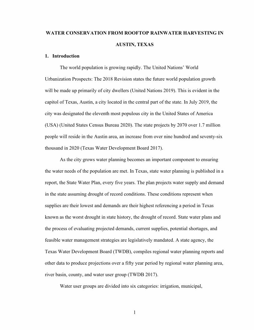
Williamson, Hays, Caldwell, Bastrop, and Burnet counties (TWDB 2020). Figure 1

illustrates the footprint of the Austin service area boundary.

16

Figure 1. Austin water system boundary. Inset in Texas for location.

3.2 Land parcels

The Texas Natural Resources Information System (TNRIS) collects geographic

data for the state. This data includes a repository of 228 of the 254 county level land

parcel datasets, as of the publication of this study. Parcel data provides this study the area

of the property, the occupancy type, and the property boundaries.

Single-family residential property land-use types were identified and extracted

from the full parcel datasets and county parcel data were merged. Travis county parcel

data classifies single-family residential properties separate from multi-family residential

properties; therefore, only single-family residential properties, classified as A1, were

17

included for analysis. Williamson county parcel data does not separate single-family and

multi-family residential properties. Manual separation of these property types was

conducted. Parcel size, property type, and verification using ancillary satellite imagery

was used to remove multi-family residential properties from single-family residential

properties. Hays County parcels were not included in this study due to a lack of land-use

type in the dataset. Only a small portion of the Austin water system boundary is in Hays

County with an estimated six hundred parcels being excluded. Burnet, Bastrop, and

Caldwell county parcels were also not included in this study due to the small number of

parcels (less than one hundred) within the water system boundary. Additionally, an even

smaller number of these properties are small enough to meet the maximum parcel size

used in this study.

Sample properties were selected during the supervised classification process to

calculate land-use percentages. These samples represented a median single-family

residential size lot, 0.2 acres, calculated from the full single-family residential dataset.

Only properties like the sample properties were sought for this study. Properties with a

legal area greater than 0.5 acres were removed from analysis. Over 236,000 parcels meet

these criteria (TNRIS 2019). Figure 2 shows a sample view of single-family residential

parcels with 0.5 acres or less on top of orthoimagery from a sample area tile, discussed

later.

18

Figure 2. Single-family parcels of 0.5 acres or less example from northwest Montopolis orthoimagery tile.

Limitations do exist when using parcel polygon features in GIS. Parcels do not

cover all the property that may be irrigated by the homeowner. For instance, a parcel

polygon feature may not cover the area from the street curb to the sidewalk, but grass

may exist here. This small area of irrigable land should not largely influence the

calculation of outdoor water demand. Additionally, even after reprojection of the parcel

shapefiles, property lines observed in the orthoimagery do not accurately align with

parcel lines in all places. Sample parcels were chosen for their near accurate alignment.

This misalignment should not significantly influence the rainwater harvesting calculation

19

because the sum of all parcels’ legal area was used, and collective and individual parcel

landscaped area was adjusted by multiplying the average percent of landscaped area from

sample parcel areas.

3.3 Building footprints

Microsoft’s open source computer generated building footprints of Texas were

obtained from their GitHub repository (Microsoft 2019). The data format was adjusted

from GeoJSON to shapefile using ArcGIS Pro 2.7.2 and projected to match the parcel

dataset. A North American Datum (NAD) 1983 Texas Statewide Mapping System

projected coordinate system with a Lambert Conformal Conic projection was used.

Building footprint polygon features provide the area of the catchment surface, the

roof. The area of the roof is multiplied by the average monthly rainfall, in gallons per

square feet, to calculate the potential volume of water from the collection area. A runoff

coefficient is applied to this volume to determine the estimated supply to the collection

tank. Using the intersect tool in ArcGIS Pro, 202,074 single-family residential parcels

with 0.5 acres or less intersect building footprints. The building footprints dataset was

joined with intersecting parcels to establish total catchment area and total parcel area.

Figure 3 shows a sample view of building footprints.

20

Figure 3. Single-family building footprints on parcels of 0.5 acres or less in northwest Montopolis orthoimagery tile.

There are limitations in using these computer-generated building footprints to

determine catchment area. The building footprints do not accurately align with footprints

of buildings observed from orthoimagery. In most cases the computer-generated building

footprints are smaller than the actual footprint meaning the calculations of catchment area

are undervalued in this study however, this can only mean a greater potential could be

realized if building footprints with greater accuracy were available. Typically, the

computer-generated footprints do not include detached structures, like storage sheds, or

roof covered porch areas. The difference in actual to computer-generated building

21

footprints was determined to have only minor effect on the outcome of the study.

3.4 Precipitation and evapotranspiration

Rainfall is the most important variable in the rainwater harvesting. Calculating the

potential volume of water from the collection area requires the volume of average rainfall

for the region. Precipitation data was obtained from the monthly climate normals

determined by the National Oceanic and Atmospheric Administration (NOAA) (see table

1). The Austin Camp Mabry station was used as it represented a central location in the

study area. Between 1981 and 2010, the Austin area averaged 34 inches of precipitation,

or 21 gallons per square foot (NOAA 2011). The average rainfall is also used to

determine total monthly demand of irrigated areas. Rainfall directly on irrigated areas

decreases the demand from the rainwater harvesting system.

Table 1. Average monthly rainfall totals for Camp Mabry station in central Austin, Texas.

Month Average

rainfall (in.) Month Average rainfall (in.)

January 2.22 July 1.88 February 2.02 August 2.35 March 2.76 September 2.99 April 2.09 October 3.88 May 4.44 November 2.96 June 4.33 December 2.40

Annual 34.32

Source: Data from NOAA 2011.

Note: Average of 1981 to 2010 climate normals.

Evapotranspiration is the volume of water plants need to grow. Texas A&M

AgriLife Extension calculates a standard evapotranspiration rate for different stations

22

across Texas. The Austin (LCRA Redbud) weather station’s Potential Evapotranspiration

of a Grass Reference Crop (ETo) averages were used. Over 70 years of climatic data

determine the ETo for this station. Table 2 shows the Austin area averages over 57 inches

of ETo annually (Texas A&M AgriLife Extension 2021). Figure 4 illustrates the

relationship between rainfall and ETo.

Table 2. Average monthly evapotranspiration for LCRA (Redbud) station in Austin, Texas.

Month Average evapotranspiration (in.) Month Average

evapotranspiration (in.) January 2.27 July 7.22 February 2.72 August 7.25 March 4.34 September 5.57 April 5.27 October 4.38 May 6.39 November 2.74 June 7.15 December 2.21

Annual 57.51

Source: Data from Texas A&M AgriLife Extension 2021. Note: Average of 70 years of evapotranspiration data.

23

Figure 4. Stacked line chart of average monthly rainfall and average monthly evapotranspiration for weather stations in Austin, Texas.

A plant water use coefficient is multiplied by the average ETo to determine the

average plant water needs, 34 inches or 21 gallons per square foot annually. The

difference between average rainfall and average plant water needs coupled with the size

of the landscaped area provides outdoor irrigation demand. Calculated annually, average

rainfall and average plant water needs are almost identical. However, when calculated

monthly there are times when plant water needs are lower than rainfall and vice versa

(see figure 5). For example, the summer season has low rainfall and significantly higher

ETo; plants require more water in the hotter summer months.

24

Figure 5. Stacked line chart of average monthly plant water needs and average monthly rainfall in Austin, Texas.

3.5 Runoff and plant water use coefficients

Seven tiers of coefficients correspond to the primary type of roofing material:

metal or glass, rubber, asphalt shingle, tar and gravel, cement tile, clay tile, or green roof.

These constitute runoff coefficients between 0.95 for metal or glass and 0.28 for green

roof (TWDB 2010). The higher the coefficient the more water can be collected from the

roof material assuming the gutter and collection system are installed correctly. The Roof-

Reliant Landscaping Manual states “asphalt shingle roofs, which are very popular

because they are relatively inexpensive, can be efficient for water harvesting” (Downey

2009). For this study asphalt shingle is used as the primary roof material when

considering the runoff coefficient. Observations from orthoimagery during supervised

classification suggest this is the primary roof material in the study area. The coefficient is

0.9, meaning it is a relatively efficient roof material for rainwater harvesting.

Suitable grasses for the central Texas climate include bermuda, paspalum, St.

25

Augustine, zoysia, and buffalo. These turf grass can tolerate summer heat and high

humidity and require little to no supplemental irrigation (Chalmers and McAfee 2010).

Five tiers of coefficients correspond to plant water use: very low, low, medium, high, and

very high. Very low corresponds to desert like plants, medium corresponds to most warm

climate turf grasses and trees, and very high corresponds to garden vegetables. A plant

water use coefficient is multiplied by the average ETo to calculate outdoor water use

demand. Some properties in the study area have xeriscape or desert-like landscaped areas

and some properties have gardens for growing vegetables. On one end of the spectrum is

very low outdoor water use demand and on the other is very high outdoor water use

demand. Most properties in the study area have turf grass covering much of the

landscaped area of their property. A medium plant water use coefficient, 0.6, was used

for this study corresponding to the primary component, and average, of landscaped areas

in the study area. The term landscaped area is used throughout referring to areas of a

property requiring supplemental irrigation where rainfall does not meet plant water needs,

assumed as a majority turf grass in this study.

3.6 Water use

Austin reports annually on the water production and usage in TWDB’s water use

survey. In 2019, over fifty billion gallons of surface water was produced or purchased.

Over two and a half billion gallons were sold to other water systems and over forty-one

billion gallons were sold to retail customers or used by the utility. Over fourteen billion

gallons of the forty-one billion was sold to 214,949 single-family residential connections.

The number of parcels, before intersecting with building footprints, discussed earlier

26

exceeds the number of single-family connections listed in Austin’s annual water use

survey (2019). This may be due to differences in the classification of properties between

the water system and the appraisal district.

An average of 68,203 gallons of water are used annually per connection.

Appendix A provides a copy of the 2019 Water Use Survey. The outdoor use as a

percentage of total use from Hermitte and Mace (2012), stated above, is 33 percent for

Austin. Of the 68,203 gallons annually used per connection, roughly 22,506 gallons

would be estimated as outdoor use. This represents a significant volume of water which

could be conserved from the use of rainwater harvesting and other conservation

techniques.

3.7 Orthoimagery and land-use classification

Orthoimagery of the study area was used to conduct supervised land

classification. Land-use classification of sample areas provided an average percent land

cover of landscaped areas. The average landscaped-area land-use percentage provided an

estimated area of turf grass for 202,074 single-family residential properties in the Austin

service area, representing 94 percent of the single-family residential accounts identified

in the water use survey from 2019 (City of Austin 2019).

Orthoimagery was collected from TNRIS’s Strategic Mapping Program’s

CapArea Imagery 2019. The imagery was flown during leaf-off conditions in January

2019 providing 6-inch pixel spatial resolution tiles with 4-band spectral resolution

(RGBIR). Each pixel represents 6-inch spatial resolution which provides very detailed

imagery to identify small features. Features in residential properties such as cars,

27

sidewalks, fences, and gardens are all identifiable with this level of resolution (Strategic

Mapping Program 2019).

The orthoimagery collected is packaged in sets of tiles. Each tile set contains

multiple tiles, representing one square mile per tile. Each tile represents a section of

imagery flown during the CapArea Imagery project. One tile from each tile set, a total of

six, were selected. Using ESRI’s ArcGIS Pro 2.7.2, land-use classification was performed

in a sample of individual single-family residential parcels from the six tiles within the

study area.

To best represent most single-family residential properties in Austin, the six tiles

were chosen by performing a kernel density spatial analysis on points created from over

236,000 single-family residential building footprints within Austin. Kernel density

calculates the density of point or polyline features per unit area (ESRI 2021). Figure 6

shows the density of these points per square mile of the Austin water system boundary

classified into ten equal interval classes. The darker the color the denser the single-family

residential buildings per square mile.

28

Figure 6. Kernel density of building footprint points per square mile classified into ten equal-interval classes.

The six tiles chosen from TNRIS tile sets correspond to a high density of single-

family residential homes as represented in the kernel density spatial analysis. These tiles

are named by TNRIS for their location. They are all located within the Austin water

system boundary though the name may not suggest. The tiles include northeast Oak Hill,

northwest Oak Hill, northwest Montopolis, east southeast Austin, east northwest Austin,

and west southwest Pflugerville (Strategic Mapping Program 2019). Figure 7 shows the

location of these six tiles.

.

29

Figure 7. TNRIS orthoimagery tile locations. Each polygon is the name of the original orthoimagery tile set: (a) west southwest Pflugerville, (b) east northwest Austin, (c) east southeast Austin, (d) northeast Oak Hill, (e) northwest Oak Hill, and (f) northwest Montopolis.

4. Method

Building footprint square footage, precipitation, and a runoff coefficient provide

data for a rainwater harvesting system supply. Evapotranspiration, precipitation,

landscaped area square footage, and a plant water use coefficient provide data for the

outdoor water demand of landscaped areas. Irrigated area square footage is not a readily

available dataset. Parcel square footage is available, however. An object-based,

supervised land-use classification using ESRI’s ArcGIS Pro was conducted on sample

30

areas within the selected orthoimagery tiles. Other ArcGIS Pro tools were used in pre-

processing and post-processing of the orthoimagery tiles. From the classified images,

sample parcels were selected to calculate the average percent of landscaped area.

4.1 Supervised classification

Object-based, supervised classification is a machine learning method that

segments a multiband remote sensing image then acquires user training inputs that

represent land cover types selected from a classification schema to classify an image.

Image segmentation groups similar neighboring pixel values together into objects. From

this segmented image, the user inputs the observed land cover type from the classification

schema. From these training samples the software classifies the objects based on their

similarity to the training pixel values within the image. Some land cover features are

identified incorrectly, either from a low number of training samples per land cover type

or the land cover types pixel values being more like other land cover types than their own

class. An accuracy assessment, further discussed below, is calculated identifying the class

assignment accuracy. To elaborate, the assessment identifies which land cover features

were classified incorrectly and what class they were placed in by the machine learning

model. The image can then be reclassified by the user to correct any observed errors

(ESRI 2021).

Using ESRI’s ArcGIS Pro tool, Create Features, polygon features were created

within each location tile representing sample areas with a high density of single-family

residential homes, per the kernel density spatial analysis. These sample areas were

extracted using the polygon features as mask. Figure 8 shows the six sample areas.

31

Figure 8. Orthographic imagery of extracted residential areas used for supervised classification in six orthoimagery areas within Austin Water boundary: (a) west southwest Pflugerville, (b) east northwest Austin, (c) east southeast Austin, (d) northeast Oak Hill, (e) northwest Oak Hill, and (f) northwest Montopolis.

Object-based, supervised classifications was performed on each of the six sample

areas. First segmentation was performed, while maintaining the clipping extent, with a

spectral detail of 15.5, a spatial detail of 15, and a minimum segment size in pixels of 5.

Spectral detail is the level of significance the user chooses to give to the difference in

spectral characteristics of pixels on a scale of 1.0 to 20.0 when identifying object

segments. A higher spectral detail directs the model to create smaller object segments

representing high detail of varying classes, and vice versa (ESRI 2021). A relatively high

value was used to reduce grouping grass, tree, and green hue features into the same object

segment. Spatial detail is the level the user defines so the program can determine whether

32

a proximate pixel should be included with neighboring pixels when creating object

segments. A range of 1 to 20 is used where a higher value indicates small and clustered

pixels of varying classes exist in relative proximity (ESRI 2021). A relatively high spatial

value was used to distinguish between buildings and roads as separate classes. A

minimum size of segment relates to the limit at which the program should merge

segments below the minimum size with best-fitting neighboring segments (ESRI 2021).

After segmentation, the user manually selected land cover types per the

classification schema. The classification schema was user generated for the purpose of

this study and included land cover types found in single-family residential

neighborhoods. It included light, medium, and dark colored buildings (or roofs), light and

dark colored roads (or other non-roof impervious covers like sidewalks and driveways),

trees, pools, and turf grass. Between 50 and 150 objects were classified by the user per

land cover type from the schema as training samples.

Shadows were also included, as large portions of parcels were covered in

shadows. An average of between 5 and 15 percent of the sample parcels’ area, within the

sample areas, were covered by shadow after classification. Shadows make it difficult to

identify the actual land cover type without ground truth data; however, reclassification

was conducted on sample parcels and shadows were removed before obtaining the

percent of landscaped area.

After user input training samples, the images were trained using the machine

learning model support vector machine. A maximum number of samples per class of 500

was selected to train the classifier. Once training was complete, the images were

classified per the training model. Light, medium, and dark colored buildings and light and

33

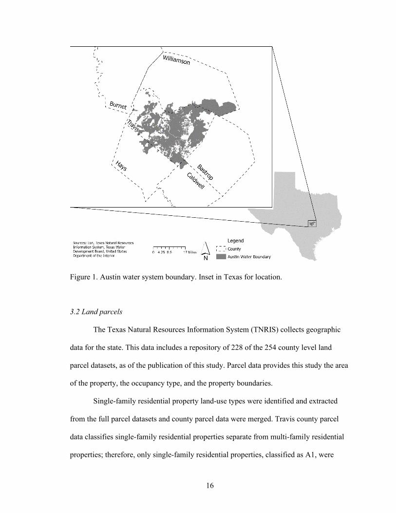
dark colored roads were then merged into buildings and roads, respectively, to combine

like features. Figure 9 shows the classified images of the sample areas. Appendix B

provides higher detailed versions of these classified images.

Figure 9. Orthographic imagery of extracted residential areas classified in six orthoimagery areas within Austin Water boundary: (a) west southwest Pflugerville, (b) east northwest Austin, (c) east southeast Austin, (d) northeast Oak Hill, (e) northwest Oak Hill, and (f) northwest Montopolis.

To identify errors in the classified images, over 100 accuracy assessment points

were generated for each sample-area classified image. Each point was manually assigned

a ground truth value corresponding to the classification schema. The user hides the

classified value and assigns the ground truth value with the aid of the original

orthoimagery and ancillary data (e.g., Google Earth Pro 7.3.3.7786) (Gao 2009). A

34

stratified random-sample method accuracy assessment was performed on over 100 points

of the ground truthed accuracy assessment points (Gao 2009, ESRI 2021). The accuracy

assessment produced a table, known as a confusion matrix, of the accuracy of the

classifier in classifying land cover type (Gao 2009). The six individual confusion

matrices, shown in appendix C, show an overall accuracy between 58.7 and 77.3 percent.

The west southwest Pflugerville tile sample area confusion matrix, shown in table

3, provides an example of the overall and individual land cover type accuracies. The

overall accuracy is 77.3 percent. An overall accuracy is calculated from the sum of the

diagonal accurately classified points divided by the total classified points (Gao 2009).

Table 3. West-southwest Pflugerville tile sample area confusion matrix.

Pool Roof Road Tree Grass Shadow Total User’s Accuracy

Kappa

Pool 9 1 0 0 0 0 10 90% Building 0 16 1 0 7 0 24 67% Road 0 1 18 0 0 0 19 95% Tree 0 3 0 10 0 1 14 71% Grass 0 1 1 6 23 1 32 72% Shadow 0 1 0 1 0 9 11 82% Total 9 23 20 17 30 11 110 Producer’s Accuracy 100% 70% 90% 59% 77% 82% 77.3%

Kappa 0.72

A user’s and producer’s accuracy are calculated for each individual land cover

type. The user’s accuracy shows where land-use types were erroneously classified, or

included, in another class (Gao 2009). For example, the computer classified nine non-

grass land-uses incorrectly as grass. An accuracy of 72 percent of classified land types

were correctly classified as grass. The producer’s accuracy shows where land-use types

35

were erroneously classified as other land-use types (Gao 2009). For example, the

computer excluded seven non-grass land-use types from the grass land-use type. An

accuracy of 77 percent of classified grass types were classified correctly as grass, or 23

percent of points were classified as buildings but were grass in this example. A user’s

accuracy of 72 percent and a producer’s accuracy of 77 percent indicate a moderate

accuracy of classification for the grass land-use type. Individually, the sample imagery

tiles’ user’s accuracy ranges from 50 to 76 percent and producer’s accuracy ranges from

67 to 100 percent.

Congalton (2001) explains a Cohen’s kappa coefficient, or kappa coefficient, is

also calculated with the accuracy assessment. A kappa coefficient shows the agreement

between the classified image and the reference image classification results on a scale of

zero to one. The more agreement between the classified and reference image, the closer a

kappa coefficient will be to one; with less of an agreement, the kappa coefficient will be

closer to zero. A kappa coefficient value below 0.4 represents poor agreement, a value of

0.4 to 0.8 constitutes a moderate agreement, and a value above 0.8 constitutes a strong

agreement (Congalton 2001). In this study, the Cohen’s kappa coefficient ranged from

0.5 to 0.72 across the six sample imagery tiles. This indicates the classification of all

samples were within moderate agreement with the expected outcome for land-use type.

4.2 Reclassification and landscaped area square footage

A moderate accuracy for classification of turf grass could be higher for this study.

Accuracy assessment identified most of the errors in classifying grass were classified as

trees and vice versa. This could be due to tree spectral characteristics similar to turf grass

36

spectral characteristics (Gao 2009). From observation, trees over turf grass should not

significantly affect the usefulness of the turf grass area from being irrigated from

rainwater harvesting systems or receiving precipitation. To correct this and obtain a more

accurate percent of parcel covered by turf grass, random points were generated within

each imagery tile. Ten parcels from each sample area orthoimagery tile were selected

corresponding to the random points. A total sixty parcels were extracted from the sample

areas using the parcels as the mask. Pixel counts were then collected for each land-use

type.

Each of the 60 parcels were reclassified using ESRI’s ArcGIS Pro tool, Pixel

Editor. Manual correction was applied to these areas using observation of the original

orthoimagery and ancillary data. All shadows and trees were reclassified as the observed

feature below. For instance, areas with trees over grass area were reclassified using

images from Google Earth Pro, where tree leaf density was lower compared to the

orthoimagery used in this study and grass areas could be observed. Other misclassified

areas were reclassified as their observed land cover type. A recount of the pixels was

performed with the reclassified images. Figure 10 shows the progression of a sample

parcel from original orthoimagery to classified to reclassified using the above method.

37

Figure 10. Progression of a sample parcel from orthoimagery to classified to reclassified.

After reclassification, grass area became the landscaped area. The percentage of

landscaped area coverage per parcel was calculated by dividing the number of landscaped

area pixels from the total parcel pixel count. An average of all sixty parcels’ percent

landscaped area coverage was then calculated to be 60 percent. This percentage was

applied to the total legal area of the 202,074 parcels in the study, 1.87 billion square feet.

The landscaped area was calculated as 1.1 billion square feet across all parcels in the

study area.

38

4.3 Outdoor demand

Calculating outdoor demand in landscaped areas is dependent on climate, soil,

and plant type. Plant water needs are calculated using a plant water use coefficient

multiplied by ETo (Texas A&M AgriLife Extension 2021). Plant water needs are

typically met in wetter months, with sufficient rainfall, or during a dormant growth

period and associated low demand. ETo data is expressed in inches per month. To adjust

to the unit of area for the landscaped area, square feet, ETo is converted to gallons per

square feet per month by multiplying ETo by 0.62 gallons per square foot. The following

equations are adapted from the Texas Rainwater Harvesting Calculator (TWDB 2010).

Equation (1.1) shows average plant water needs, Naw, is equal to average monthly

potential evapotranspiration of a grass reference crop, ETom, multiplied by the plant

water use coefficient, PWUcoeff, then adjusted to gallons per square feet, by multiplying

by 0.62 (gallons per square foot).

𝑁𝑁𝑎𝑎𝑎𝑎 = 𝐸𝐸𝐸𝐸𝐸𝐸𝑚𝑚 × 𝑃𝑃𝑃𝑃𝑃𝑃𝑐𝑐𝑐𝑐𝑐𝑐𝑐𝑐𝑐𝑐 × 0.62 (1.1)

Equation (1.2) calculates the monthly outdoor demand of plants. Monthly outdoor

demand (gallons), Dom, is equal to Naw multiplied by the total landscaped area (square

feet), AIrr.

𝐷𝐷𝑐𝑐𝑚𝑚 = 𝑁𝑁𝑎𝑎𝑎𝑎 × 𝐴𝐴𝑖𝑖𝑖𝑖𝑖𝑖 (1.2)

Equation (1.3) calculates the monthly potential volume of water from rainfall

directly on landscaped areas. The potential volume of water from rainfall directly on

landscaped areas (gallons), Pim, is equal to AIrr multiplied by the product of average

monthly rainfall (inches), Rm, and 0.62 gallons per square foot.

𝑃𝑃𝑖𝑖𝑚𝑚 = 𝐴𝐴𝑖𝑖𝑖𝑖𝑖𝑖 × (𝑅𝑅𝑚𝑚 × 0.62) (1.3)

39

Equation (1.4) represents the total monthly irrigation demand of landscaped areas.

Total monthly irrigation demand (gallons), Dtmi, is equal to Dom minus Pim.

𝐷𝐷𝑡𝑡𝑚𝑚𝑖𝑖 = 𝐷𝐷𝑐𝑐𝑚𝑚 − 𝑃𝑃𝑖𝑖𝑚𝑚 (1.4)

If Pim is greater than Dom, then Dtmi would equal zero. A negative Dtmi is not

appropriate for this calculation therefore Dtmi would equal zero. Monthly rainfall may

meet or exceed demand in one month, but this volume is not banked. In subsequent

months plants require additional rainfall or irrigation. This is important when calculating

total annual irrigation demand. It is the sum of Dtmi, not the difference of annual potential

volume of water from rainfall directly on landscaped areas (sum of Pim) and annual

outdoor demand of plants (sum of Dom) (see appendix D).

4.4 Collected supply

The potential volume of water on the catchment area provides a starting point for

determining the volume that can be supplied to storage tanks for use on landscaped areas.

The type of roof materials and whether the roof is pitched are factors in the efficiency of

rainfall being collected from rooftops. The area of the rooftop, volume of rainfall, and a

runoff coefficient provide the estimated supply to the storage tanks.

Equation (2.1) shows the potential volume of water from the collection area, Vcam,

is equal to building footprint (square feet), BFa, multiplied by the product of Rm and 0.62

gallons per square feet.

𝑉𝑉𝑐𝑐𝑎𝑎𝑚𝑚 = 𝐵𝐵𝐵𝐵𝑎𝑎 × (𝑅𝑅𝑚𝑚 × 0.62) (2.1)

Equation (2.2) shows the monthly supply to collection tank (gallons), Sectm, is

equal to Vcam multiplied by the runoff coefficient, ROcoeff.

40

𝑆𝑆𝑐𝑐𝑐𝑐𝑡𝑡𝑚𝑚 = 𝑉𝑉𝑐𝑐𝑎𝑎𝑚𝑚 × 𝑅𝑅𝑅𝑅𝑐𝑐𝑐𝑐𝑐𝑐𝑐𝑐𝑐𝑐 (2.2)

5. Results and Discussion

As mentioned, rainwater harvesting requires a supply to meet eventual demand.

Supply calculations require minimal data manipulation, and the inputs are readily

available with some customization. Demand estimation requires knowledge of the study

area. Though most inputs are readily available, estimating the size of landscaped areas

required machine learning techniques using orthoimagery with high spatial resolution.

This step in the process provides the most room for error. The percent coverage of an

average parcel was calculated and found to be like sample parcels. Areas of land-use

types were reasonably correct when compared to their sample to obtain an estimate of

landscaped area.

5.1 Outdoor demand

The 202,074 parcels in this study, representing 94 percent of single-family

connections in Austin, cover 1.9 billion square feet. The average single-family parcel is

9,256 square feet. The average percent of landscaped area, obtained from object-based

supervised classification of sample parcels, is 60 percent. Sixty percent of the 1.9 billion

square feet of the parcels’ lot size was classified as landscaped area, 1.1 billion square

feet. The average landscaped area of a single-family parcel is 5,553 square feet.

The annual outdoor demand from landscaped areas is 24 billion gallons,

calculated as the sum of Dom. The potential volume of water from rainfall that falls

directly on landscaped areas is 23.9 billion gallons, calculated as the sum of Pim. As

41

discussed earlier, the difference between the annual figures is not used because supply

and demand vary by season or month. For instance, there is a deficit of rainfall for

landscaped area plant water needs in April, July, August, and September, using the

average of 30 years of rainfall data (NOAA 2011). In Austin, apparently the adage April

showers bring May flowers does not apply, unless irrigation is provided. The sum of the

total monthly irrigation demand, Dtmi, for these four months is 4.1 billion gallons. This

volume represents how much supplemental water is needed from harvested/stored

rainwater to irrigate landscaped areas at single-family residential properties in Austin

beyond what average rainfall provides.

5.2 Collected supply

Single-family residential building footprints cover nearly 470 million square feet

of catchment area in Austin. An average single-family parcel’s building(s) covers 2,326

square feet. The annual potential volume of water from the collection area is 10 billion

gallons, calculated from the sum of Vcam. Including the runoff coefficient of 0.9 for

asphalt shingle roof material, 9 billion gallons of water is the supply available for

collection, calculated from the sum of Sectm. This amount represents the volume of water

all 202,074 single-family residential parcel buildings in Austin can supply.

5.3 How much water can be collected and conserved?

If all houses identified in this study had the proper rainwater harvesting

equipment, 9 billion gallons of water could be collected. If homeowners only irrigated

their landscaped area with the volume of water the plants need then nearly 4.1 billion

42

gallons could be conserved from the potable water system. An average storage tank of

12,500 gallons would be necessary at each house if each homeowner wanted to meet all

plant water needs in all months with harvested rainwater alone. A smaller tank would not

be sufficient to capture and store enough water to meet outdoor irrigation demand. Stated

earlier, Tamaddun, Kaira, and Ahmad (2018) found a 1,000 gallon storage capacity is not

sufficient to meet water use demand during dry months.

Some homes do not irrigate their landscaped areas and may not need to irrigate

depending on their landscape-plant types, while others may overwater their landscaped

area resulting in more water than necessary being used for irrigation (EPA 2013, Landon,

Kyle and Kaiser 2016). A 2012 report by the TWDB found the average outdoor water use

as a percentage of total water use for Austin was 33 percent, using water use data from

2004 to 2011 (Hermitte and Mace 2012). This percent can be applied to an adjusted 2019

volume of total water use for Austin. The houses in this study represent 94 percent of the

214,949 single-family properties in the annual water use survey (City of Austin 2019).

Adjusting the 14 billion gallons of the collective single-family residential usage in the

2019 annual water use survey (City of Austin 2019) and multiplying by 94 percent yields

an approximate 13.8 billion gallons of total water usage for the 202,074 properties in this

study.

Thirty-three percent of the 13.8 billion gallons of the collective single-family

residential adjusted usage in 2019 is approximately 4.5 billion gallons. By this

calculation, roughly 459 million gallons of water is used beyond the average plant water

needs at these properties. Even if properties overwater their landscaped areas, with a

collected supply of 9 billion gallons, from a 12,500 gallon tank, there is adequate supply,

43

a surplus of over 4.5 billion gallons, for plant water needs and other uses. Homeowners

could water their turf grass twice as much as the estimated outdoor irrigation demand

illustrated by Hermitte and Mace (2012) and over two times the plant water needs using

collected rainwater with a cistern size of 12,500 gallons at each home in this study. This

surplus water, if captured could be used for other purposes beyond outdoor irrigation.

Table 4 illustrates the comparison of outdoor irrigation demand between watering for

plant water needs versus overwatering at 33 percent of total water use for the collective

single-family residential properties.

Table 4. Comparison of collective single-family residential outdoor irrigation demand.

Outdoor water use

Annual single-family residential

total water use (gallons)

Annual single-family residential outdoor irrigation demand (gallons)

Estimated supply to storage tanka

(gallons)

Plant water needs metb 13,781,275,140 4,088,353,476 8,999,521,267

33 percent of total usec 13,781,275,140 4,547,820,796 8,999,521,267

Difference - 459,467,320 a Assuming a 12,500 gallon storage tank. b If plant water needs were met with rainfall and rainwater harvesting, illustrated from this study’s calculations. c If 33 percent of total household water use was used outdoors, illustrated by Hermitte and Mace (2012).

A total water savings from rainwater harvesting systems and the difference in

outdoor irrigation demand between two studies may illustrate findings relevant to water

planning regions and governments; however, it is also of concern how this could be

implemented for the average household. The average annual total water demand of a

single-family residential property in Austin, calculated from the collective adjusted total

44

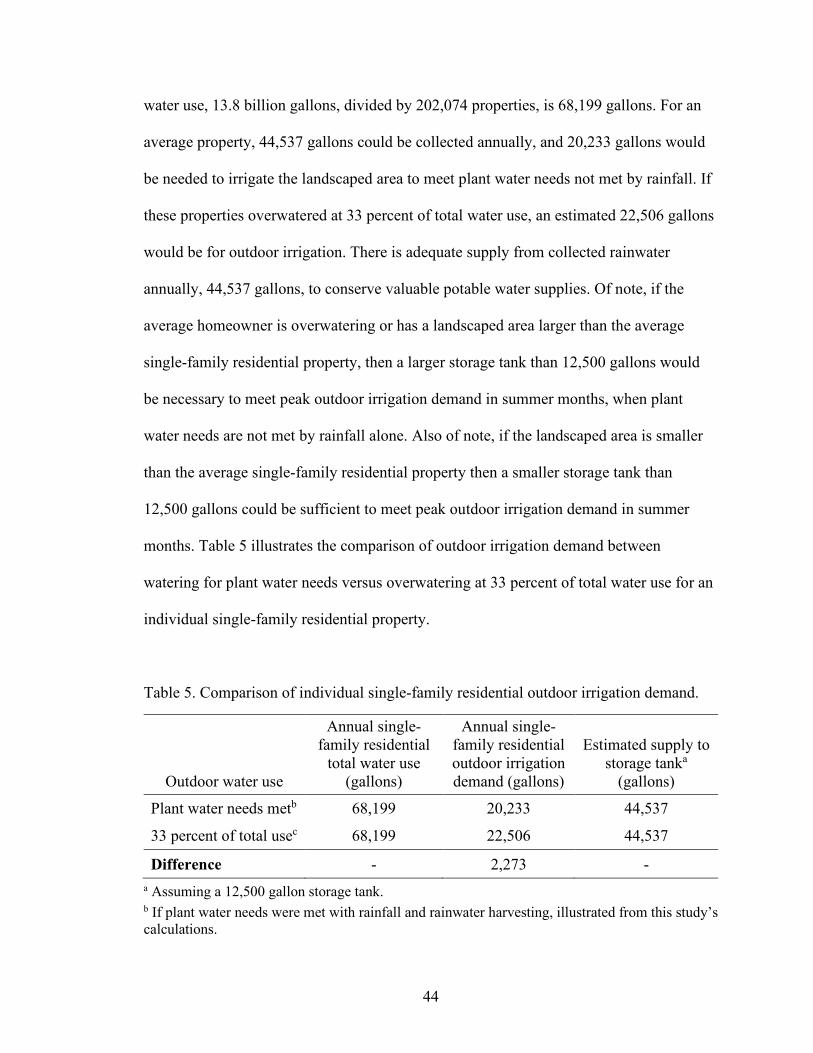
water use, 13.8 billion gallons, divided by 202,074 properties, is 68,199 gallons. For an

average property, 44,537 gallons could be collected annually, and 20,233 gallons would

be needed to irrigate the landscaped area to meet plant water needs not met by rainfall. If

these properties overwatered at 33 percent of total water use, an estimated 22,506 gallons

would be for outdoor irrigation. There is adequate supply from collected rainwater

annually, 44,537 gallons, to conserve valuable potable water supplies. Of note, if the

average homeowner is overwatering or has a landscaped area larger than the average

single-family residential property, then a larger storage tank than 12,500 gallons would

be necessary to meet peak outdoor irrigation demand in summer months, when plant

water needs are not met by rainfall alone. Also of note, if the landscaped area is smaller

than the average single-family residential property then a smaller storage tank than

12,500 gallons could be sufficient to meet peak outdoor irrigation demand in summer

months. Table 5 illustrates the comparison of outdoor irrigation demand between

watering for plant water needs versus overwatering at 33 percent of total water use for an

individual single-family residential property.

Table 5. Comparison of individual single-family residential outdoor irrigation demand.

Outdoor water use

Annual single-family residential

total water use (gallons)

Annual single-family residential outdoor irrigation demand (gallons)

Estimated supply to storage tanka

(gallons)

Plant water needs metb 68,199 20,233 44,537

33 percent of total usec 68,199 22,506 44,537

Difference - 2,273 - a Assuming a 12,500 gallon storage tank. b If plant water needs were met with rainfall and rainwater harvesting, illustrated from this study’s calculations.

45

c If 33 percent of total household water use was used outdoors, illustrated by Hermitte and Mace (2012).

A 12,500 gallon storage tank takes up a large footprint of the landscaped area.

This size tank would require either a minimum diameter of 12 feet at a height of around

16 feet or a minimum diameter of 18 feet at a height of around 8 feet (TWDB 2005). A

12-foot diameter tank would cover a minimum of 113 square feet of area while an 18 foot

diameter tank would cover a minimum of 254 square feet of area (see figure 11). The

average property has an estimated 9,256 square foot lot and 5,553 square feet of

landscaped area available for a tank with these diameters. Ultimately a storage tank could

reduce the area required for irrigation and provide a catchment area for rainwater.

However, the height of these tanks is not feasible at most properties because of the size

limitations on a property. Additionally, tall structures could require the removal or

transfer of trees or other land features on many properties, unsightly and large structures

may lower the aesthetics of the property, and tall structures are potential hazards should

they collapse, falling on and/or flooding homes.

46

Figure 11. Comparison of storage tank diameters on average sized study area parcel.

An alternative to a single large structure is installing two or more storage tanks

equivalent to 12,500 gallons of storage. The use of multiple storage tanks could alleviate

the burden of storage tank and rainwater harvesting appurtenances maintenance. During

April, June, July, and August outdoor irrigation demand is high; however, during the

other months of the year the storage tanks are refilling, and plant water needs are met by

rainfall without supplemental irrigation. Taking a storage tank off-line during this period

for maintenance may be more manageable for a homeowner, the proprietor of the

rainwater harvesting system and components. Installing two or more storage tanks also

reduces the area of landscape to be irrigated, a negative feedback loop. Additionally,

47

situating multiple storage tanks at different sides of a home can increase roof runoff and

conduit efficiency by reducing travel distance from catchment and storage. If two 6,250

gallon storage tanks were installed, each tank would still have a footprint with a diameter

of 12 feet or roughly 113 square feet, but with a height of 8 feet or less; that is, each tank

is half as tall as a 12,500 gallons storage tank with the same diameter footprint. For

reference, the percent reduction in landscaped area from installing two tanks is less than 5

percent of the average properties’ landscaped area, resulting in a very low decrease in

outdoor irrigation demand.

Replacing the landscaped area with low water use plants, a drought tolerant or

native landscape, can also reduce the outdoor irrigation demand. By reducing the outdoor

irrigation demand, the size of the tank can be reduced. For example, drought tolerant or

native landscapes water demand can be met by rainfall without the need for supplemental

irrigation (Tamaddun, Kaira and Ahmad 2018), reducing the need for a larger storage

tank. Austin provides a rebate of up to $1,750 for its residential customers to replace a

minimum of 500 square feet of turf grass with native and adapted plants. The converted

area must have at least 50 percent plant coverage when plants are mature (City of Austin

2021). Other areas have set similar requirements or set limitations for the installation of a

drought tolerant landscape. In Nevada, a maximum of 50 percent of the side and rear

landscaped area of a property can be converted to a drought tolerant landscape

(Tamaddun, Kaira and Ahmad 2018).

Assuming 12,500 gallons of storage were installed on a property, conversion of a

portion of the landscaped area to drought tolerant or native landscape would yield a

reduction in the annual outdoor irrigation demand. Table 6 shows the average properties

48

annual outdoor irrigation demand, the volume of outdoor irrigation demand not met by

12,500 gallons of storage (i.e., deficit), the months with a deficit, represented by the

number for the month (i.e., 1 = January), and the volume of potable water conserved by

using rainwater in the storage tank. Even without converting any portion of the

landscaped area to a drought tolerant or native landscape no deficit in water exists

because this size of storage is adequate to meet peak outdoor irrigation demand in the

drier months and not drawdown the storage to empty, as expressed in Tamaddun, Kaira,

and Ahmad (2018).

Table 6. Outdoor irrigation demand conserved by 12,500 gallons of storage before and after landscape conversion on an average Austin single-family residential property.

Landscaped area converted

(% | sq. ft.)

Annual outdoor irrigation demand

(gallons)

Annual deficit of

water (gallons)

Months with a deficit

Annual volume conserved by

storage (gallons)

0 | 0 20,233 - - 20,233

10 | 555 18,208 - - 18,208

25 | 1,388 15,173 - - 15,173 50 | 2,777 10,116 - - 10,116 75 | 4,165 5,058 - - 5,058

Note: Annual volume conserved decreases due to lower demand from conversion of landscaped area to low water use plants.

Another alternative is to compound reducing the storage size and replacing a

portion of the landscaped area with drought tolerant or native plants. Using the rainwater

harvesting calculations and adjusting for the conversion of landscaped area to drought

tolerant landscape, a minimum tank size can be calculated. If 50 percent of the average

property were converted, a 5,000 gallon tank would still be required to meet plant water

49

needs over all months of the year. Up to 10,116 gallons of potable water could be

conserved. A 5,000 gallon storage tank would still require at least a 12-foot diameter tank

at a height of 6 feet. Two 2,500 gallon storage tanks would require at least a 6-foot

diameter footprint at a height of 12 feet. Table 7 shows the average properties annual

outdoor irrigation demand, the volume of outdoor irrigation demand not met by 5,000

gallons of storage (i.e., deficit), the months with a deficit, represented by the number for

the month (i.e., 1 = January), and the volume of potable water conserved by using

rainwater in the storage tank.

Table 7. Outdoor irrigation demand conserved by 5,000 gallons of storage before and after landscape conversion on an average Austin single-family residential property.

Landscaped area converted

(% | sq. ft.)

Annual outdoor irrigation demand

(gallons)

Annual deficit of

water (gallons)

Months with a deficit (number for month, i.e., 1 = January)

Annual volume conserved by

storage (gallons)

0 | 0 20,233 7,280 7, 8 12,953 10 | 555 18,208 5,746 7, 8 12,462

25 | 1,388 15,173 3,446 7, 8 11,727 50 | 2,777 10,116 - - 10,116 75 | 4,165 5,058 - - 5,058

Note: Annual volume conserved decreases due to lower demand from conversion of landscaped area to low water use plants.

A 1,000 gallon tank used in the calculations by Tamaddun, et al. (2018), could be

appropriate for many homeowners. At a diameter of 6 feet only 24 square feet of space is

required. At a height of six feet a 1,000 gallon tank is more manageable and less likely to

create a hazard on the property. For comparison, a 10-foot diameter above-ground pool at

a 3-foot depth holds more water than these tanks. Table 8 shows an average properties’

50

annual outdoor irrigation demand, the volume of outdoor irrigation demand not met by

1,000 gallons of storage (i.e., deficit), the months with a deficit, represented by the

number for the month (i.e., 1 = January), and the volume of potable water conserved by

using rainwater in the storage tank.

Table 8. Outdoor irrigation demand conserved by 1,000 gallons of storage before and after landscape conversion on an average Austin single-family residential property.

Landscaped area converted

(% | sq. ft.)

Annual outdoor irrigation demand

(gallons)

Annual deficit of

water (gallons)

Months with a deficit (number for month, i.e., 1 = January)

Annual volume conserved by

storage (gallons)

0 | 0 20,233 16,233 4, 7, 8, 9 4,000 10 | 555 18,208 14,208 4, 7, 8, 9 4,000

25 | 1,388 15,173 11,264 4, 7, 8 3,909 50 | 2,777 10,116 6,510 4, 7, 8 3,606 75 | 4,165 5,058 1,832 7, 8 3,226

Note: Annual volume conserved decreases due to lower demand from conversion of landscaped area to low water use plants.

These results illustrate there can be many components to computing the outdoor

irrigation volume conserved through rainwater collection. The volume of water from

rainfall, the area of roofs available for rainwater catchment, the area of landscapes, the

type of plants on the landscape, the plant water needs, the volume of storage required to

store the rainwater, the size of the storage that is appropriate for the property, and so on.

It may require a lot of data, but the benefits of rainwater harvesting are high, including

the conservation of potable water resources. Depending on a homeowner’s tank size and

landscape preference, between 3,226 and 20,233 gallons could be conserved. A larger

volume of storage can provide adequate supply to meet outdoor irrigation demand in dry

51

times and conserve large volumes of potable water. Also, compounding rainwater

harvesting with a landscape conversion to drought tolerant or native plants can result in a

decreased outdoor irrigation demand, a decrease in the volume of outdoor irrigation

demand not met by stored rainwater (i.e., deficit), and a decrease in the number of

months with a deficit, if a homeowner installs a tank without adequate storage to meet

outdoor irrigation demand without landscape conversion.

6. Conclusion

This study presents a method for calculating rainwater harvesting potential supply

and outdoor irrigation demand volumes. Collective single-family residential parcels,

202,074, and individual single-family residential parcels were analyzed to determine

these volumes. The calculations and GIS techniques performed, in this project report, on

various data sources produced results showing a significant volume of water could be

collected to supplant and therefore conserve potable water supply in Austin.

This study found a collective and individual volume of water, nearly 9 billion

gallons and 44,537 gallons, respectively, could be collected with adequately sized

storage. This volume exceeds plant water needs; therefore, a storage capacity of 12,500

gallons, at an average single-family residence, is necessary to meet outdoor irrigation

demand in all months of the year. With adequately sized storage to meet outdoor

irrigation in all months of the year a collective and individual total volume of water,

nearly 4.1 billion gallons and 20,233 gallons, respectively, of water could be conserved.

Collectively and individually a surplus of rainfall on roofs, 4.9 billion gallons and 24,304

gallons, respectively, exists due to lower outdoor irrigation demand than the potential

52

volume of rainfall collected from roof.

Additionally, due to storage and property limitations, it is appropriate to consider

the potential versus reality of rainwater harvesting systems for conserving potable water

supply in Austin. Rainfall may be plenty to meet outdoor irrigation demands using

rooftop rainwater harvesting with leftover supply for other water uses; however, storage

space and size may be a limiting factor for many homeowners. Reducing the storage size,

or splitting the storage capacity across multiple tanks, can still provide water supply for

outdoor irrigation demand and result in conservation of potable water supply; though, a

deficit of water may exist in some months if demand exceeds supply. It may be necessary

to consider combining rainwater harvesting with other conservation strategies, such as

landscape conversion. This study found, by increasing drought tolerant and native plants

outdoor irrigation demand decreased resulting in less needed supply/storage. The right

combination of conservation strategies is necessary to meet demands in all months of the

year.

Further study is warranted to determine the volume of other demands besides

outdoor irrigation, identify other storage alternatives, and develop other costs and

benefits of rooftop rainwater harvesting in Austin. Additionally, it is important to note,

rooftops exist on other properties besides single-family residences. Multi-family

residential, commercial, and industrial properties exist in Austin as well. These sites may

have greater potential for rainwater harvesting due to their larger building footprints.

They may also have more resources and land area to accommodate larger storage

facilities for rainwater. Another study could assess their potential among these and other

factors. Finally, rooftops are not the only catchment surfaces in the study area. Further

53

research could identify the potential for rainwater harvesting from non-rooftop surfaces.

Rainwater harvesting has a history of use and a great potential for offsetting water

demand on public water supplies. It should be implemented more broadly by

homeowners and utilities to achieve sustainable water supply. Additionally, state,

regional, and local governments and other stakeholders should continue to research the

potential of this alternate supply of water.

54

References Chalmers, David R, and James McAfee. 2010. Turfgrass Selection for Texas. Publication,

Bryan: Texas AgriLife Extension. City of Austin. 2021. Rebates, Free Stuff & Grants. Accessed March 15, 2021.

https://www.austintexas.gov/department/rebates-free-stuff-grants. —. 2019. 2019 City of Austin Water Use Survey. Water Use Survey, Austin: Texas Water

Development Board. —. 2018. Water Forward Integrated Water Resource Plan. Plan, Austin: City of Austin.

Accessed April 27, 2021. https://www.austintexas.gov/waterforward. Congalton, Russell. 2001. "Accuracy assessment and validation of remotely sensed and

other spatial information." International Journal of Wildland Fire, 10: 321-328. DeOreo, William B., Peter W. Mayer, Leslie Martien, Matthew Hayden, Andrew Funk,

Michael Kramer-Duffield, Renee Davis, et al. 2011. California single-family water use efficiency study. Report, Prepared for California Department of Water Resources.

Downey, Nate. 2009. Roof-Reliant Landscaping: Rainwater Harvesting with Cistern Systems in New Mexico. Manual, New Mexico Office of the State Engineer.

ESRI. 2021. ArcGIS Pro. Accessed January 12, 2021. https://pro.arcgis.com. —. 2021. The Image Classification Wizard. Accessed January 11, 2021.

https://pro.arcgis.com/en/pro-app/latest/help/analysis/image-analyst/the-image-classification-wizard.htm.

Gage, Edward, and David J. Cooper. 2015. "The Influence of Land Cover, Vertical Structure, and Socioeconomic Factors on Outdoor Water Use in a Western US City." Water Resources Management, 29: 3877-3890.

Gao, Jay. 2009. "Classification Accuracy Assessment, Chapter 12." In Digital Analysis of Remotely Sensed Imagery, by Jay Gao. The McGraw-Hill Companies, Inc. 2009.

Gleick, Peter H., Dana Haasz, Christine Henges-Jeck, Veena Srinivasan, Gary Wolff, Katherine Kao Cushing, and Amardip Mann. 2003. Waste Not, Want Not: The potential for urban water conservation in California. Pacific Institute for Studies in Development, Environment, and Security.

Haq, Syed Azizul. 2017. Harvesting Rainwater from Buildings. Switzerland: Springer International Publishing.

Hermitte, Sam Marie, and Robert E. Mace. 2012. The Grass is Always Greener... Outdoor Residential Water Use in Texas. Technical Note 12-01, Austin: Texas Water Development Board.

Herrmann, Thilo, and Uwe Schmida. 1999. "Rainwater utilisation in Germany: efficiency, dimensioning, hydraulic and environmental aspects." Urban Water, 4 (1): 307-316.

Hof, Angela, and Nils Wolf. 2014. "Estimating potential outdoor water consumption in private urban landscapes by coupling high-resolution image analysis, irrigation water needs and evaporation estimation in Spain." Landscape and Urban Planning, 123: 61-72.

Hoseini, S. H., and V. Attarzadeh Hosseini. 2020. "Rainwater Harvesting in Residential Areas of Arid and Semi-Arid Regions (Case Study: Torbat-E Jam, Iran)." Desert, 25 (2): 130-138.

Imteaz, Monzur Alam, Amimul Ahsan, and Abdallah Shanableh. 2013. "Reliability

55

analysis of rainwater tanks using daily water balance model: Variations within a large city." Resources, Conservation and Recycling, 77: 37-43.

Landon, Adam C, Gerard T Kyle, and Ronald A Kaiser. 2016. "Predicting compliance with an information-based residential outdoor water conservation program." Journal of Hydrology, 536: 26-36.

Lower Colorado Regional Water Planning Group. 2016. 2016 Region K Water Plan. Regional Water Plan, Austin: Lower Colorado Regional Water Planning Group.

Manikandan, M., M. V. Ranhaswami, and G. Thiyagarajan. 2011. "Estimation of Rooftop Rain Water Harvesting Potential by Water Budgeting Study." International Journal of Finance & Economics, 2 (1): 36-41.

Mathieu, Renaud, Claire Freeman, and Jagannath Aryal. 2007. "Mapping private gardens in urban areas using object-oriented techniques and very high-resolution satellite imagery." Landscape and Urban Planning, 81 (3): 179-192.

Mehrabadi, Mohammad Hossein Rashidi, Bahram Saghafian, and Fereshte Haghighi Fashi. 2013. "Assessment of residential rainwater harvesting efficiency for meeting non-potable water demands in three climate conditions." Resources, Conservation and Recycling, 73: 86-93.

Microsoft. 2019. US Building Footprints. Accessed May 24, 2020. https://github.com/Microsoft/USBuildingFootprints.

Mini, C., T. S. Hogue, and S. Pincetl. 2014. "Estimation of residential outdoor water us in Los Angeles, California." Landscape and Urban Planning (127): 124-135.

Nachshon, Uri, Lior Netzer, and Yakov Livshitz. 2016. "Land cover properties and rain water harvesting in urban environments." Sustainable Cities and Society (Elsevier) 27: 398-406.

National Oceanic and Atmospheric Administration [NOAA]: National Centers for Environmental Information. 2011. "Austin Camp Mabry, Tx US Monthly Normals." Data Tools: 1981-2010 Normals. Accessed January 29, 2021. https://www.ncdc.noaa.gov/cdo-web/datatools/normals.

Ojwang, Robert O, Jorg Dietrich, Prajna Kasargodu Anebagilu, Matthias Beyer, and Franz Rottensteiner. 2017. "Rooftop Rainwater Harvesting for Mombasa: Scenario Development with Image Classification and Water Resources Simulation." Water 359 (9): 1-19.

Strategic Mapping Program. 2019. CapArea Imagery. Accessed January 15, 2021. https://data.tnris.org/collection/f84442b8-ac2a-4708-b5c0-9d15515f4483.

Tamaddun, Kazi, Ajay Kaira, and Sajjad Ahmad. 2018. "Potential of rooftop rainwater harvesting to meet outdoor water demand in arid regions." Journal of Arid Land (February): 68-83.

Texas A&M AgriLife Extension. 2021. "Historic ETo Reference." TexasET Network. Accessed February 15, 2021. https://texaset.tamu.edu/.

Texas Natural Resources Information System [TNRIS]. 2019. Land Parcels 2019. Accessed December 27, 2020. https://data.tnris.org/collection/2679b514-bb7b-409f-97f3-ee3879f34448.

Texas Parks and Wildlife Department. 2021. Hueco Tanks State Park & Historic Site. Accessed February 21, 2021. https://tpwd.texas.gov/state-parks/hueco-tanks/park_history.

Texas Rainwater Harvesting Evaluation Committee [TRHEC]. 2006. Rainwater

56

Harvesting Potential and Guidelines for Texas. Report to the 80th Legislature, Austin: Texas Water Development Board.

Texas Water Development Board. 2020. Texas Water Service Boundary Viewer. Accessed December 4, 2020. https://www.twdb.texas.gov/waterplanning/waterusesurvey/serviceboundaryeditor.asp.

—. 2017. "2017 Texas State Water Plan." Texas State Water Plan. Accessed January 27, 2021.

—. 2016. A Watering Guide for Texas Landscapes. Brochure, Austin: Texas Water Development Board.

—. 2010. "Rainwater Harvesting Document - Resources: TWDB Rainwater Calculator v2.0." Texas Water Development Board. Accessed December 27, 2020. https://www.twdb.texas.gov/innovativewater/rainwater/docs.asp.

—. 2005. The Texas Manual on Rainwater Harvesting. Manual, Austin: Texas Water Development Board.

United Nations, Department of Economic and Social Affairs, Population Division. 2019. World Urbanization Prospects: The 2018 Revision (ST/ESA/ESR.A/420). New York: United Nations.

United States Census Bureau. 2020. "Southern and Western Regions Experienced Rapid Growth this Decade." United States Census Bureau. Accessed February 4, 2021. https://www.census.gov/newsroom/press-releases/2020/south-west-fastest-growing.html.

United States Environmental Protection Agency [EPA]. 2013. Water-Smart Landscapes: Start with WaterSense. Brochure, EPA WaterSense Program, United States Environmental Protection Agency. Accessed March 12, 2021. https://www.epa.gov/sites/production/files/2017-01/documents/ws-outdoor-water-efficient-landscaping.pdf.

United States Geological Survey. 2021. "What is a digital orthophoto quadrangle (DOQ) or orthoimage?" United States Geological Survey. Accessed 04 20, 2021. https://www.usgs.gov/faqs/what-a-digital-orthophoto-quadrangle-doq-or-orthoimage.

Villar-Navascues, Ruben, Alfredo Perez-Morales, and Salvador Gil-Guirado. 2020. "Assessment of Rainwater Harvesting Potential from Roof Catchments through Clustering Analysis." Water 2623 (12): 1-14.

57

APPENDIX A City of Austin, Annual Water Use Survey (2019)

58

59

60

61

APPENDIX B Six Study Sample Area Classified Images

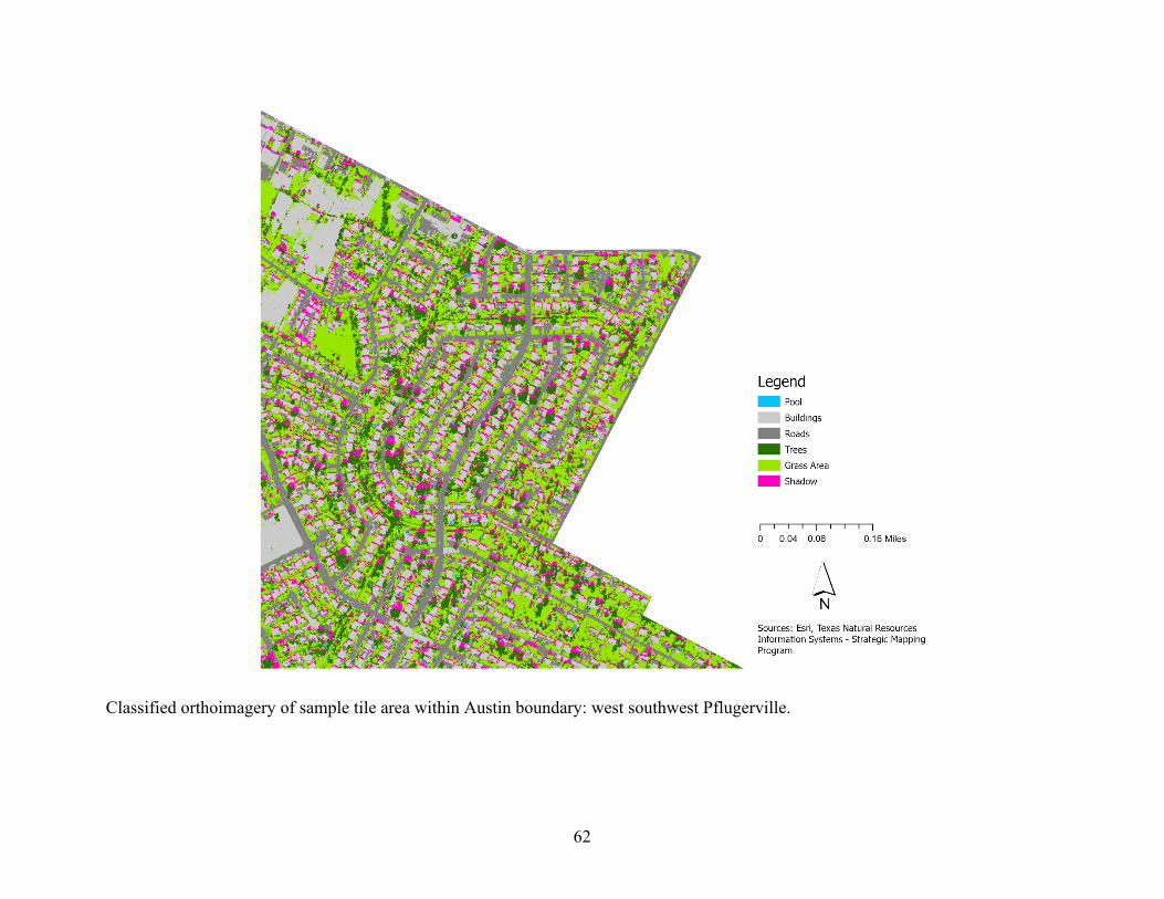
62

Classified orthoimagery of sample tile area within Austin boundary: west southwest Pflugerville.

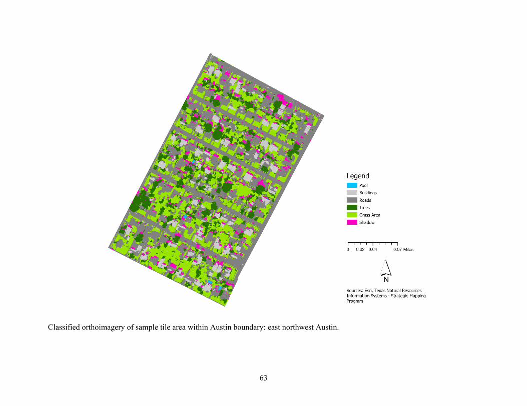
63

Classified orthoimagery of sample tile area within Austin boundary: east northwest Austin.

64

Classified orthoimagery of sample tile area within Austin boundary: east southeast Austin.

65

Classified orthoimagery of sample tile area within Austin boundary: northeast Oak Hill.

66

Classified orthoimagery of sample tile area within Austin boundary: northwest Oak Hill.

67

Classified orthoimagery of sample tile area within Austin boundary: northwest Montopolis.

68

APPENDIX C Six Study Sample Area Classified Image Confusion Matrices

69

West southwest Pflugerville confusion matrix

Pool Roof Road Tree Grass Shadow Total User’s Accuracy

Kappa

Pool 9 1 0 0 0 0 10 90.0% Roof 0 16 1 0 7 0 24 66.7% Road 0 1 18 0 0 0 19 94.7% Tree 0 3 0 10 0 1 14 71.4% Grass 0 1 1 6 23 1 32 71.9% Shadow 0 1 0 1 0 9 11 81.8% Total 9 23 20 17 30 11 110 Producer’s Accuracy

100.0% 69.6% 90.0% 58.8% 76.7% 81.8% 77.3%

Kappa 0.72 East northwest Austin confusion matrix

Pool Roof Road Tree Grass Shadow Total User’s Accuracy

Kappa

Pool 10 0 0 0 0 0 10 100.0% Roof 0 10 0 0 0 0 10 100.0% Road 0 15 15 4 4 5 43 34.9% Tree 0 0 0 9 2 3 14 64.3% Grass 0 0 0 6 20 3 29 68.9% Shadow 0 0 1 0 0 9 10 90.0% Total 10 25 16 19 26 20 116 Producer’s Accuracy

100.0% 40.0% 93.8% 47.4% 76.9% 45.0% 62.9%

Kappa 0.55 East southeast Austin confusion matrix

Pool Roof Road Tree Grass Shadow Total User’s Accuracy

Kappa

Pool 8 2 0 0 0 0 10 80.0% Roof 0 10 7 1 0 1 19 52.6% Road 0 4 11 1 0 0 16 68.8% Tree 0 0 0 9 1 0 10 90.0% Grass 0 2 3 13 25 2 45 55.6% Shadow 0 0 0 4 1 9 14 64.3% Total 8 18 21 28 27 12 114 Producer’s Accuracy

100.0% 55.6% 52.4% 32.1% 92.6% 75.0% 63.2%

Kappa 0.55

70

Northeast Oak Hill confusion matrix

Pool Roof Road Tree Grass Shadow Total User’s Accuracy

Kappa

Pool 3 7 0 0 0 0 10 30.0% Roof 0 14 2 1 0 0 17 82.4% Road 0 12 12 4 0 0 28 42.9% Tree 0 0 0 10 0 0 10 100.0% Grass 0 2 0 14 17 1 34 50.0% Shadow 0 0 1 1 0 8 10 80.0% Total 3 35 15 30 17 9 109 Producer’s Accuracy

100.0% 40.0% 80.0% 33.3% 100.0% 88.9% 58.7%

Kappa 0.50 Northwest Oak Hill confusion matrix

Pool Roof Road Tree Grass Shadow Total User’s Accuracy

Kappa

Pool 2 3 3 1 1 0 10 20.0% Roof 0 16 2 0 0 0 18 88.9% Road 0 1 13 0 0 0 14 92.9% Tree 0 1 3 14 5 0 23 60.9% Grass 0 2 1 6 16 0 25 64.0% Shadow 0 3 0 4 2 11 20 55.0% Total 2 26 22 25 24 11 110 Producer’s Accuracy

100.0% 61.5% 59.1% 56.0% 66.7% 100.0% 65.5%

Kappa 0.58 Northwest Montopolis confusion matrix

Roof Road Tree Grass Shadow Total User’s Accuracy

Kappa

Roof 21 4 1 1 0 27 77.8% Road 7 8 0 2 0 17 47.1% Tree 2 0 16 4 1 23 69.6% Grass 1 1 4 19 0 25 76.0% Shadow 0 0 0 0 10 10 100.0% Total 31 13 21 26 11 102 Producer’s Accuracy

67.7% 61.5% 76.2% 73.1% 90.9% 72.5%

Kappa 0.65

71

APPENDIX D Collective and Individual Single-Family Residential Rainwater Harvesting

Calculations (Austin)

72

Collective single-family residential rainwater harvesting calculation (Austin).

Month

Average monthly

rainfall (gal. per sq. ft.)

Estimated monthly supply

to collection tank (gal.)

Average plant water needs

(gal. per sq. ft.)

Monthly outdoor demand

(gal)

Potential volume of water from rainfall directly on irrigated

areas (gal.)

Total monthly demand (gal.)

January 1.38 582,136,865 0.84 947,640,816 1,544,612,784 - February 1.25 529,692,103 1.01 1,135,499,128 1,405,458,479 - March 1.71 723,737,724 1.61 1,811,789,049 1,920,329,407 - April 1.3 548,047,769 1.96 2,200,029,560 1,454,162,486 745,867,074 May 2.75 1,164,273,730 2.38 2,667,588,024 3,089,225,568 - June 2.68 1,135,429,111 2.66 2,984,859,839 3,012,690,700 - July 1.17 492,980,769 2.69 3,014,082,243 1,308,050,466 1,706,031,777 August 1.46 616,225,961 2.70 3,026,606,131 1,635,063,082 1,391,543,049 September 1.85 784,049,201 2.07 2,325,268,434 2,080,356,858 244,911,576 October 2.41 1,017,428,395 1.63 1,828,487,566 2,699,593,514 - November 1.84 776,182,487 1.02 1,143,848,386 2,059,483,712 - December 1.49 629,337,152 0.82 922,593,041 1,669,851,658 - Annual 21.28 8,999,521,267 21.39 24,008,292,217 23,878,878,714 4,088,353,476

Coefficients and areas Values

Parcel area (sq. ft.) 1,870,353,560 Irrigation area (sq. ft.) 1,122,212,136 Building footprint (sq. ft.) 469,935,149 Runoff coefficient 0.9 Plant water use coefficient 0.6

73

Individual single-family residential rainwater harvesting calculation with an average 12,500 gallons of storage (Austin).

Month

Average monthly rainfall (gal. per sq. ft.)

Estimated monthly supply to collection tank (gal.)

Average plant water needs (gal. per sq. ft.)

Monthly outdoor

demand (gal)

Potential volume of water from rainfall directly on irrigated

areas (gal.)

Total monthly demand (gal.)

Estimated volume of

water left in tank (or

deficit) at end of month (gal)

January 1.38 2,881 0.84 4,690 7,644 - 2,881 February 1.25 2,621 1.01 5,619 6,955 - 5,502 March 1.71 3,582 1.61 8,966 9,503 - 9,084 April 1.3 2,712 1.96 10,887 7,196 3,691 8,105 May 2.75 5,762 2.38 13,201 15,288 - 12,500 June 2.68 5,619 2.66 14,771 14,909 - 12,500 July 1.17 2,440 2.69 14,916 6,473 8,443 4,057 August 1.46 3,050 2.70 14,978 8,091 6,887 220 September 1.85 3,880 2.07 11,507 10,295 1,212 2,888 October 2.41 5,035 1.63 9,049 13,359 - 7,923 November 1.84 3,841 1.02 5,661 10,192 - 11,764 December 1.49 3,114 0.82 4,566 8,264 - 12,500 Annual 21.28 44,537 21.39 118,811 118,169 20,233

Coefficients and areas Values Parcel area (sq. ft.) 9,256 Irrigation area (sq. ft.) 5,553 Building footprint (sq. ft.) 2,326 Runoff coefficient 0.9 Plant water use coefficient 0.6 Storage size (gal.) 12,500