FutureWater

Costerweg 1V

6702 AA Wageningen

The Netherlands

+31 (0)317 460050

info@futurewater.nl

www.futurewater.nl

Water Allocation Planning in Pungwe Basin

Mozambique

July 2014

Commissioned by

Partners for Water

Authors

Peter Droogers

Wilco Terink

Report FutureWater: 129

2

Contents

1 Introduction 6

1.1 Relevance 6 1.2 Pungwe Basin 7

2 Methods and Tools 8

2.1 Relevance 8 2.2 WEAP 8

3 Building WEAP for Pungwe Basin 11

3.1 Introduction 11 3.2 Model Components 11

3.2.1 Boundary, area extent and background layers 11

3.2.2 Sub-catchments 13

3.2.3 Climate 13

3.2.4 Urban and industrial demand 14

3.2.5 Minimum outflow requirement 14

3.2.6 Land cover 14

3.3 Validation and calibration 17

4 Results 20

4.1 Current situation 20 4.2 Future Developments 23 4.3 Water Infrastructure Developments 26

4.4 Daily Reservoir Operations 29

5 Conclusions and Recommendations 33

6 Selected References 34

3

Tables Table 1. Areas of the 12 sub-basins as applied in WEAP. ......................................................... 13 Table 2. Aggregated land classes of the 12 catchments as applied in WEAP. .......................... 15 Table 3. Distribution of surface water availability in Mozambique and Zimbabwe for the Pungwe

River basin based on the hydrological years 1960-80. The long-term available water

resources are judged to be 5-15% lower than the values given in the table. (Source:

SWECO, 2004). .............................................................................................................. 17 Table 4. Estimated natural runoff (MAR) for the Pungwe subbasins for the period Oct 1960 to

Sep 1981. The runoff coefficient is the ratio between MAR and MAP. The coefficient of

variation is the ratio between the standard deviation on of annual flows and the

MAR. The long-term available water resources are judged to be 5-15% lower than the

values given in the table. (Source: SWECO, 2004). ..................................................... 18

Table 5. Reservoir operational rules as explored using WEAP as an O-DSS (Operational

Decision Support System). ............................................................................................. 30

Figures

Figure 1: Location of the Pungwe River basin in central Mozambique. ........................................ 7 Figure 2: Application of models to evaluate future water resources developments based on

today’s policies. ................................................................................................................ 8

Figure 3: Relation between spatial scale and physical detail in water allocation tools. The green

ellipses show the key strength of some well-known models. (Source: Droogers and

Bouma, 2014) ................................................................................................................... 9

Figure 4. Various background layers used to support model building in WEAP. National

Geographic Base map (top), SRTM-DEM (middle), main rivers and subbasins (bottom)

........................................................................................................................................ 12 Figure 5. Example of input data: precipitation read from a text file. ............................................ 14 Figure 6. Final WEAP model of Pungwe Basin. .......................................................................... 16

Figure 7. Details of downstream area of the WEAP model for the Pungwe Basin. .................... 16 Figure 8. The figure shows the mean annual runoff for the last 50 years (Mm 3 /year). The red

line denotes the average annual river flow. The large inter-annual variation in water

resources in the Pungwe River Basin causes large demands on water management.

Dry spells, e.g. 1991-1995, create large stress on the water users. (Source: GRM, GRZ,

2006). ............................................................................................................................. 17 Figure 9. Monthly distributions of natural runoff at the river mouth. (Source: GRM, GRZ, 2006).

........................................................................................................................................ 18

Figure 10. Validation of the WEAP model: outflow observed and modeled to Indian Ocean. .... 19 Figure 11. Annual total water demand. ....................................................................................... 20

Figure 12. Monthly average water demand for the period 2001-2010. ....................................... 21 Figure 13. Annual total unmet demand (water shortage). ........................................................... 21 Figure 14. Monthly average unmet demand (water shortage) for the period 2001-2010. .......... 22

Figure 15. Monthly outflow of the basin into the ocean. .............................................................. 22 Figure 16. Beira Agricultural Growth Corridor: high potential agricultural areas. ........................ 23

Figure 17. Monthly average water demand under the three scenarios....................................... 24 Figure 18. Monthly average water shortage (unmet demand) under the three scenarios. ......... 25 Figure 19. Coverage of water demand under the three scenarios. ............................................. 25

4

Figure 20. Impact of the three BAGC scenarios on outflows of the Pungwe. The Graph shows

the reduction in flows compared to the reference condition. .......................................... 26

Figure 21. Effectiveness of developing storage capacity (Res_01 to Res_03) under the BAGC

irrigation expansion. The Graph shows the annual unmet demand............................... 27 Figure 22. Effectiveness of developing storage capacity (Res_01 to Res_03) under the BAGC

irrigation expansion. The Graph shows the average annual unmet demand over a

period of 10 years. .......................................................................................................... 28 Figure 23. Effectiveness of developing storage capacity (Res_01 to Res_03) under the BAGC

irrigation expansion. The Graph shows the coverage of water demand. ....................... 28 Figure 24. The WEAP model used as an O-DSS (Operational Decision Support System) to

explore operational rules for a proposed reservoir......................................................... 30 Figure 25. Different operations of the reservoir and its impact on reservoir volume as explored

using WEAP as an O-DSS (Operational Decision Support System). Data used for two

historic years 2005 (top) and 2006 (bottom) as demonstration. .................................... 31 Figure 26. Reservoir inflows and outflows for the management scenario “early conservation” as

explored using WEAP as an O-DSS (Operational Decision Support System). Data used

from a historic year (2005) as demonstration. ................................................................ 32

5

Preface

The Netherlands’ “Partners for Water” initiative has the objective to support the Dutch water

sector to capitalize on its technologies and expertise internationally, while simultaneously

ensure that Dutch technologies and knowledge contribute to solving world water challenges.

A call for proposal was announced by “Partners for Water” 2013. A consortium of three

Netherlands’ partners developed a proposal on request of Administração Regional de Águas do

Centro (ARA-Centro), Beira-Mozambique, under the name “Water Planning Tools to Support

Water Governance”. The project was granted on 16-May-2013 and will run from March 2013 to

September 2014.

The contract number is PVWS13001.

The project partners are:

Administração Regional de Águas do Centro (ARA-Centro), Beira-Mozambique

(beneficiary)

FutureWater, Wageningen, Netherlands (lead)

Waterschap Hunze en Aa’s, Veendam, Netherlands (consortium partner)

UNESCO-IHE, Delft Netherlands (consortium partner)

WE-Consult, Maputo, Mozambique (support partner)

6

1 Introduction

1.1 Relevance

Mozambique is experiencing a steady economic growth of 5 to 10% a year. Much of this

economic growth is related to capital-intensive international projects that are high water

demanding (aluminum smelter, hydropower, transportation, irrigation). Also the water use by the

drinking water companies grows as the cities develop, and several new irrigation schemes are

planned to increase the Mozambican food production. On the long term 190,000 ha of irrigated

agriculture will be developed in the Beira region. A substantial part of this irrigation will be

developed in the management area of ARA-Centro. Also an increase in water use by FIPAG

(Water Supply Investments and Assets Fund) Beira and the sugar estate Mafambisse is

expected along the river Pungwe. All these developments result in an increase in water demand

of 10-20% per year and this trend is expected to continue the coming decades.

Large water shortages are projected if no mitigation measures will be taken over the coming

years. In general improved water governance is needed to guarantee the ecological and

economic use of water, now and on the long term in Mozambique. ARA-Centro has to advise on

the water availability and the required measures that are needed to make this development

possible. For this advisory role hydrological models and water allocation tools are needed that

can be used to quantify the available water resources and the present and future water

demand. Only by state-of-the-art models and tools, and better trained staff, based on the

Netherlands water governance principles, ARA-Centro is able to take-up these challenges.

Moreover, ARA-Centro has expressed their ambition to become the front-runner to actually

develop and implement these water governance principles.

This report is part of the ‘Water Planning Tools to Support Water Governance’ project, which

main objective is: “Demonstrate the Netherlands water governance system to one water

management organization (ARA) in Mozambique”.

The specific objective of the hydrological component of the entire study is to perform a water

resources and demand assessment of the Pungwe River Basin in order to:

Strengthen ARA-Centro’s knowledge on the current hydrological state of the Pungwe

River Basin;

Provide ARA-Centro with knowledge on the data and tools that are available to

undertake a hydrological assessment study;

Provide ARA-Centro with a roadmap (guideline) that can be followed to undertake

hydrological assessment studies for other river basins within Mozambique.

One of the activities of this project is to introduce, refine and demonstrate the application of two

water planning tools (SWAT and WEAP) to a pilot area in the ARA-Centro management area.

This report describes the water demand and unmet demand of the water resources within the

Pungwe basin using the WEAP modeling framework.

7

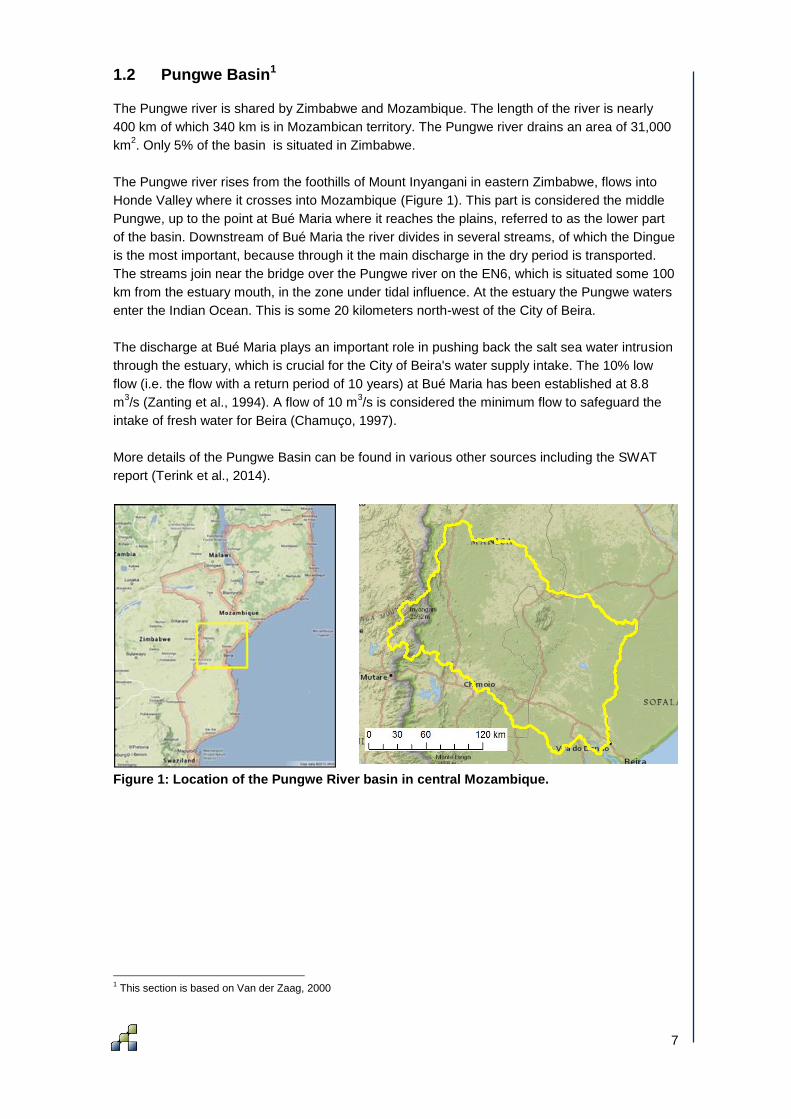
1.2 Pungwe Basin1

The Pungwe river is shared by Zimbabwe and Mozambique. The length of the river is nearly

400 km of which 340 km is in Mozambican territory. The Pungwe river drains an area of 31,000

km2. Only 5% of the basin is situated in Zimbabwe.

The Pungwe river rises from the foothills of Mount Inyangani in eastern Zimbabwe, flows into

Honde Valley where it crosses into Mozambique (Figure 1). This part is considered the middle

Pungwe, up to the point at Bué Maria where it reaches the plains, referred to as the lower part

of the basin. Downstream of Bué Maria the river divides in several streams, of which the Dingue

is the most important, because through it the main discharge in the dry period is transported.

The streams join near the bridge over the Pungwe river on the EN6, which is situated some 100

km from the estuary mouth, in the zone under tidal influence. At the estuary the Pungwe waters

enter the Indian Ocean. This is some 20 kilometers north-west of the City of Beira.

The discharge at Bué Maria plays an important role in pushing back the salt sea water intrusion

through the estuary, which is crucial for the City of Beira's water supply intake. The 10% low

flow (i.e. the flow with a return period of 10 years) at Bué Maria has been established at 8.8

m3/s (Zanting et al., 1994). A flow of 10 m

3/s is considered the minimum flow to safeguard the

intake of fresh water for Beira (Chamuço, 1997).

More details of the Pungwe Basin can be found in various other sources including the SWAT

report (Terink et al., 2014).

Figure 1: Location of the Pungwe River basin in central Mozambique.

1 This section is based on Van der Zaag, 2000

8

2 Methods and Tools

2.1 Relevance

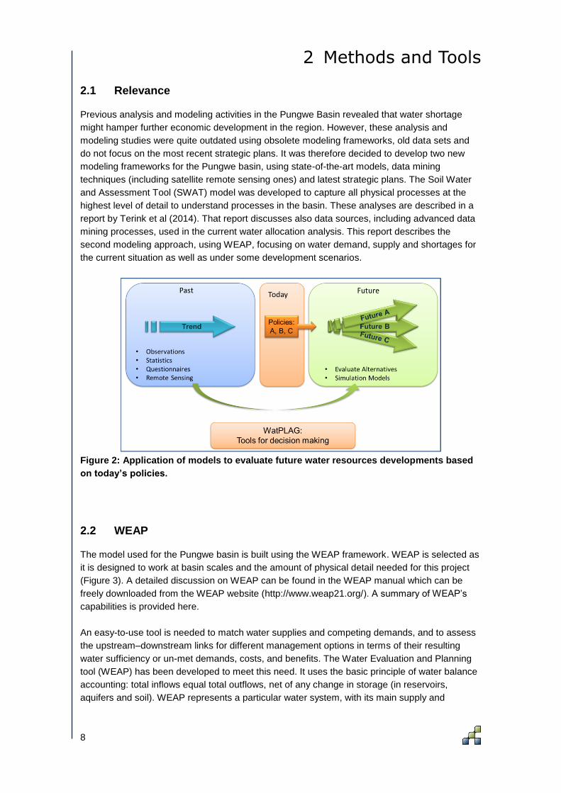
Previous analysis and modeling activities in the Pungwe Basin revealed that water shortage

might hamper further economic development in the region. However, these analysis and

modeling studies were quite outdated using obsolete modeling frameworks, old data sets and

do not focus on the most recent strategic plans. It was therefore decided to develop two new

modeling frameworks for the Pungwe basin, using state-of-the-art models, data mining

techniques (including satellite remote sensing ones) and latest strategic plans. The Soil Water

and Assessment Tool (SWAT) model was developed to capture all physical processes at the

highest level of detail to understand processes in the basin. These analyses are described in a

report by Terink et al (2014). That report discusses also data sources, including advanced data

mining processes, used in the current water allocation analysis. This report describes the

second modeling approach, using WEAP, focusing on water demand, supply and shortages for

the current situation as well as under some development scenarios.

Figure 2: Application of models to evaluate future water resources developments based

on today’s policies.

2.2 WEAP

The model used for the Pungwe basin is built using the WEAP framework. WEAP is selected as

it is designed to work at basin scales and the amount of physical detail needed for this project

(Figure 3). A detailed discussion on WEAP can be found in the WEAP manual which can be

freely downloaded from the WEAP website (http://www.weap21.org/). A summary of WEAP’s

capabilities is provided here.

An easy-to-use tool is needed to match water supplies and competing demands, and to assess

the upstream–downstream links for different management options in terms of their resulting

water sufficiency or un-met demands, costs, and benefits. The Water Evaluation and Planning

tool (WEAP) has been developed to meet this need. It uses the basic principle of water balance

accounting: total inflows equal total outflows, net of any change in storage (in reservoirs,

aquifers and soil). WEAP represents a particular water system, with its main supply and

9

demand nodes and the links between them, both numerically and graphically. Delphi Studio

programming language and MapObjects software are employed to spatially reference

catchment attributes such as river and groundwater systems, demand sites, wastewater

treatment plants, catchment and administrative political boundaries (Yates et al. 2005).

Figure 3: Relation between spatial scale and physical detail in water allocation tools. The

green ellipses show the key strength of some well-known models. (Source: Droogers and

Bouma, 2014)

Users specify allocation rules by assigning priorities and supply preferences for each node;

these preferences are mutable, both in space and time. WEAP then employs a priority-based

optimisation algorithm and the concept of “equity groups” to allocate water in times of shortage.

In order to undertake these water resources assessments the following operational steps can

be distinguished:

The study definition sets up the time frame, spatial boundary, system components and

configuration. The model can be run over any time span where routing is not a

consideration, a monthly period is used quite commonly.

System management is represented in terms of supply sources (surface water,

groundwater, inter-basin transfer, and water re-use elements); withdrawal, transmission

and wastewater treatment facilities; water demands; and pollution generated by these

activities. The baseline dataset summarises actual water demand, pollution loads,

resources and supplies for the system during the current year, or for another baseline

year.

Scenarios are developed, based on assumptions about climate change, demography,

development policies, costs and other factors that affect demand, supply and hydrology.

The drivers may change at varying rates over the planning horizon. The time horizon for

these scenarios can be set by the user.

Scenarios are then evaluated in respect of desired outcomes such as water sufficiency,

costs and benefits, compatibility with environmental targets, and sensitivity to

uncertainty in key variables.

Water supply: Using the hydrological function within WEAP, the water supply from rainfall is

depleted according to the water demands of the vegetation, or transmitted as runoff and

infiltration to soil water reserves, the river network and aquifers, following a semi-distributed,

10

parsimonious hydrologic model. These elements are linked by the user-defined water allocation

components inserted into the model through the WEAP interface.

Water allocation: The challenge is to distribute the supply remaining after satisfaction of

catchment demand the objective of maximizing water delivered to various demand elements,

and in-stream flow requirements - according to their ranked priority. This is accomplished using

an iterative, linear programming algorithm. The demands of the same priority are referred to as

“equity groups”. These equity groups are indicated in the interface by a number in parentheses

(from 1, having the highest priority, to 99, the lowest). WEAP is formulated to allocate equal

percentages of water to the members of the same equity group when the system is supply-

limited.

The concept-based representation of WEAP means that different scenarios can be quickly set

up and compared, and it can be operated after a brief training period. WEAP is being developed

as a standard tool in strategic planning and scenario assessment and has been applied in many

regions around the world.

11

3 Building WEAP for Pungwe Basin

3.1 Introduction

Building the WEAP model for Pungwe requires various sets of data. Data can be divided into

the following main categories:

Model building

o Static data2

Soils

Land use, land cover

Population

Reservoir operational rules

o Dynamic data

Climate (rainfall, temperature, reference evapotranspiration)

Water demands

Reservoir releases (if present)

Flow requirements

Model validation/calibration

o Streamflow

Data were obtained from various sources and combined into a consistent set of input for WEAP.

The following sections will summarize the building of the model, details can be found in the

model input data itself.

3.2 Model Components

3.2.1 Boundary, area extent and background layers

Within WEAP various background layers were added to support the development of the model.

These layers were created using a GIS tool such as for example ArcMap or QGIS. The most

relelvant layers that were added are (Figure 4):

Geographic based on the National Geographic World Map

Digital elevation models based on SRTM (Shuttle Radar Topography Mission)

River flow network based on the of topographic analysis using the SWAT model.

Subbasins as defined during the SWECO 2006 project.

2 Nota that static data can still vary over longer time frames, but are fairly constant over days/weeks

12

Figure 4. Various background layers used to support model building in WEAP. National

Geographic Base map (top), SRTM-DEM (middle), main rivers and subbasins (bottom)

13

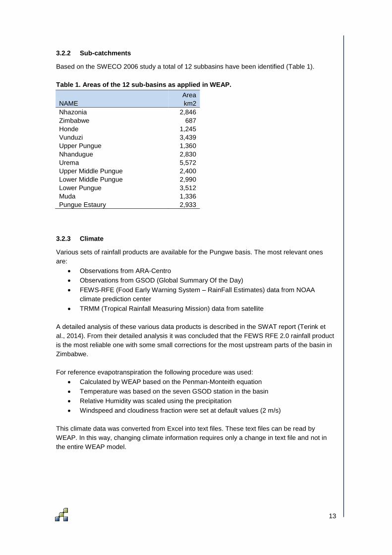
3.2.2 Sub-catchments

Based on the SWECO 2006 study a total of 12 subbasins have been identified (Table 1).

Table 1. Areas of the 12 sub-basins as applied in WEAP.

Area

NAME km2

Nhazonia 2,846

Zimbabwe 687

Honde 1,245

Vunduzi 3,439

Upper Pungue 1,360

Nhandugue 2,830

Urema 5,572

Upper Middle Pungue 2,400

Lower Middle Pungue 2,990

Lower Pungue 3,512

Muda 1,336

Pungue Estaury 2,933

3.2.3 Climate

Various sets of rainfall products are available for the Pungwe basis. The most relevant ones

are:

Observations from ARA-Centro

Observations from GSOD (Global Summary Of the Day)

FEWS-RFE (Food Early Warning System – RainFall Estimates) data from NOAA

climate prediction center

TRMM (Tropical Rainfall Measuring Mission) data from satellite

A detailed analysis of these various data products is described in the SWAT report (Terink et

al., 2014). From their detailed analysis it was concluded that the FEWS RFE 2.0 rainfall product

is the most reliable one with some small corrections for the most upstream parts of the basin in

Zimbabwe.

For reference evapotranspiration the following procedure was used:

Calculated by WEAP based on the Penman-Monteith equation

Temperature was based on the seven GSOD station in the basin

Relative Humidity was scaled using the precipitation

Windspeed and cloudiness fraction were set at default values (2 m/s)

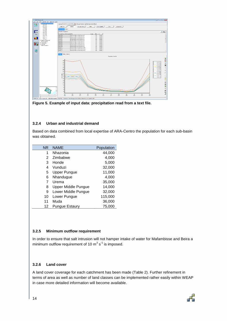
This climate data was converted from Excel into text files. These text files can be read by

WEAP. In this way, changing climate information requires only a change in text file and not in

the entire WEAP model.

14

Figure 5. Example of input data: precipitation read from a text file.

3.2.4 Urban and industrial demand

Based on data combined from local expertise of ARA-Centro the population for each sub-basin

was obtained.

NR NAME Population

1 Nhazonia 44,000

2 Zimbabwe 4,000

3 Honde 5,000

4 Vunduzi 32,000

5 Upper Pungue 11,000

6 Nhandugue 4,000

7 Urema 35,000

8 Upper Middle Pungue 14,000

9 Lower Middle Pungue 32,000

10 Lower Pungue 115,000

11 Muda 36,000

12 Pungue Estaury 75,000

3.2.5 Minimum outflow requirement

In order to ensure that salt intrusion will not hamper intake of water for Mafambisse and Beira a

minimum outflow requirement of 10 m3 s

-1 is imposed.

3.2.6 Land cover

A land cover coverage for each catchment has been made (Table 2). Further refinement in

terms of area as well as number of land classes can be implemented rather easily within WEAP

in case more detailed information will become available.

15

The Kc factor (referred to as crop factor) is used to convert the ETref (reference evapo-

transpiration) to the ETpot (potential evapotranspiration). This ETpot is subsequently used by

WEAP to calculate the ETact (actual evapotranspiration) based on the availability of water. So

as equation:

ETact = Ks ∙ ETpot

ETpot = Kc ∙ ETref

with

ETact : actual evapotranspiration (mm/d)

ETpot : potential evapotranspiration (mm/d)

ETref : reference evapotranspiration (mm/d)

Ks : reduction by water deficit (-)

Kc : crop factor (-)

Table 2. Aggregated land classes of the 12 catchments as applied in WEAP.

Area

(km2) Area (%)

NR NAME

Rainfed Irrigated Plantation Bare Shrubs Forest

1 Nhazonia 2,846 9 1 0 20 20 50

2 Zimbabwe 687 29 1 0 20 20 30

3 Honde 1,245 9 1 0 20 20 50

4 Vunduzi 3,439 9 1 0 20 30 40

5 Upper Pungue 1,360 9 1 0 20 30 40

6 Nhandugue 2,830 10 0 0 20 30 40

7 Urema 5,572 10 0 0 20 50 20

8 Upper Middle Pungue 2,400 19 1 0 20 50 10

9 Lower Middle Pungue 2,990 20 0 5 20 50 5

10 Lower Pungue 3,512 20 2 5 20 50 3

11 Muda 1,336 20 1 5 20 50 4

12 Pungue Estaury 2,933 20 5 5 20 50 0

16

Figure 6. Final WEAP model of Pungwe Basin.

Figure 7. Details of downstream area of the WEAP model for the Pungwe Basin.

17

3.3 Validation and calibration

A full validation and calibration of the hydrological SWAT model is described elsewhere (Terink,

et al., 2014). This validation/calibration of SWAT resulted in the conclusion that the model

performed well when comparing observed and simulated streamflow. To ensure that the WEAP

model, which is based on the data as used in SWAT, is also reliable, a first order validation has

been undertaken. For this the observed outflow data from the most downstream station have

been used. Since WEAP is not a fully distributed hydrological model the WEAP validation is

done on observed and simulated minimum, average and maximum monthly flows.

The overall validation of WEAP is shown in Figure 10. It is clear that WEAP is also able to

simulated observed flows. Since WEAP is a water resources model it would be desirable to

undertake another level of validation comparing observed and simulated demands and water

shortages. For this pilot project limited resources and data were available and it was therefore

not possible to undertake this second order of validation and calibration.

Figure 8. The figure shows the mean annual runoff for the last 50 years (Mm 3 /year). The

red line denotes the average annual river flow. The large inter-annual variation in water

resources in the Pungwe River Basin causes large demands on water management. Dry

spells, e.g. 1991-1995, create large stress on the water users. (Source: GRM, GRZ, 2006).

Table 3. Distribution of surface water availability in Mozambique and Zimbabwe for the

Pungwe River basin based on the hydrological years 1960-80. The long-term available

water resources are judged to be 5-15% lower than the values given in the table. (Source:

SWECO, 2004).

18

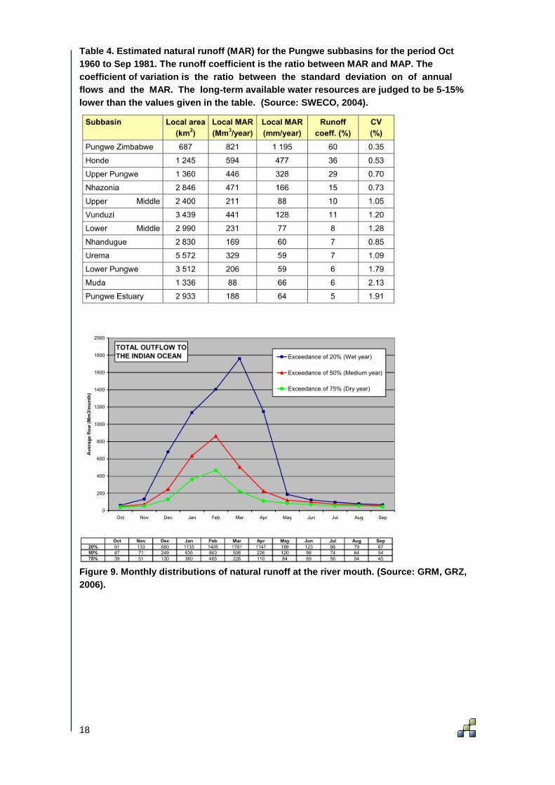
Table 4. Estimated natural runoff (MAR) for the Pungwe subbasins for the period Oct

1960 to Sep 1981. The runoff coefficient is the ratio between MAR and MAP. The

coefficient of variation is the ratio between the standard deviation on of annual

flows and the MAR. The long-term available water resources are judged to be 5-15%

lower than the values given in the table. (Source: SWECO, 2004).

Figure 9. Monthly distributions of natural runoff at the river mouth. (Source: GRM, GRZ,

2006).

19

Figure 10. Validation of the WEAP model: outflow observed and modeled to Indian

Ocean.

20

4 Results

4.1 Current situation

The WEAP model as described in the previous sections is used to assess current water

demands and shortages. As reference the period 2001-2010 was used and analyses were

undertaken at monthly time scales. Industrial and domestic demands were considered to be

constant over each year, while demands for irrigation are scaled towards the actual needs

based on climate data and crop characteristics.

Results of the WEAP runs reflecting the current situation will be mainly presented in figures and

tables. A summary of these outputs is provided here.

Total annual average demand for water withdrawals in the basin is about 550 MCM.

Some year-to-year variation exist and during wet years demand can go down to about

520 MCM, while under dry years this demand can be almost 600 MCM. (Figure 11)

A large monthly variation in water demands exist where during the month April to

November demands are much higher compared to the period December to March.

(Figure 12)

Annual average water shortage (unmet demand) is about 15 MCM. Comparing this to

the total demand means a shortage of only a few percentages. This shortage is not the

same for every year and varies substantially from zero in some years up to about 40

MCM in dry years. Monthly unmet demand is highest for August, September and

October. (Figure 13 and Figure 14)

Outflow from the basin is highly variable. Large variation exists with flows down to 7 m3

s-1

and during some months flow can go up to 1000 m3 s

-1. Note that these numbers are

monthly averages and daily flows can be substantially lower and higher. Recalculating

these cubic meters per second to millimeters shows that average long-term outflow

from the basin is 140 mm per year. (Figure 15)

All Others

Mafambisse

Dom_10

Catch_12

Catch_11

Catch_10

Catch_08

Catch_05

Catch_04

Catch_03

Catch_02

Catch_01

Beira

Water Demand (not including loss, reuse and DSM)

Scenario: Reference, All months (12)

2001 2002 2003 2004 2005 2006 2007 2008 2009 2010

Million C

ubic

Mete

r

600

550

500

450

400

350

300

250

200

150

100

50

0

Figure 11. Annual total water demand.

21

All Others

Mafambisse

Dom_10

Catch_12

Catch_11

Catch_10

Catch_08

Catch_05

Catch_04

Catch_03

Catch_02

Catch_01

Beira

Water Demand (not including loss, reuse and DSM)

Scenario: Reference, Monthly Average

January March April May June July August October December

Million C

ubic

Mete

r

80

75

70

65

60

55

50

45

40

35

30

25

20

15

10

5

0

Figure 12. Monthly average water demand for the period 2001-2010.

All Others

Mafambisse

Dom_12

Dom_10

Dom_04

Dom_01

Catch_12

Catch_10

Catch_08

Catch_05

Catch_04

Catch_03

Catch_01

Unmet Demand

Scenario: Reference, All months (12)

2001 2002 2003 2004 2005 2006 2007 2008 2009 2010

Million C

ubic

Mete

r

42

40

38

36

34

32

30

28

26

24

22

20

18

16

14

12

10

8

6

4

2

0

Figure 13. Annual total unmet demand (water shortage).

22

All Others

Mafambisse

Dom_12

Dom_10

Dom_04

Dom_01

Catch_12

Catch_10

Catch_08

Catch_05

Catch_04

Catch_03

Catch_01

Unmet Demand

Scenario: Reference, Monthly Average

January March April May June July August October December

Million C

ubic

Mete

r

7.5

7.0

6.5

6.0

5.5

5.0

4.5

4.0

3.5

3.0

2.5

2.0

1.5

1.0

0.5

0.0

Figure 14. Monthly average unmet demand (water shortage) for the period 2001-2010.

50 \ Reach

Streamflow (below node or reach listed)

Scenario: Reference, All months (12), River: Pungue

Jan

2001

Jul

2001

Jan

2002

Jul

2002

Jan

2003

Jul

2003

Jan

2004

Jul

2004

Jan

2005

Jul

2005

Jan

2006

Jul

2006

Jan

2007

Jul

2007

Jan

2008

Jul

2008

Jan

2009

Jul

2009

Jan

2010

Jul

2010

Cubic

Mete

rs p

er

Seco

nd

1,100

1,000

900

800

700

600

500

400

300

200

100

0

Figure 15. Monthly outflow of the basin into the ocean.

23

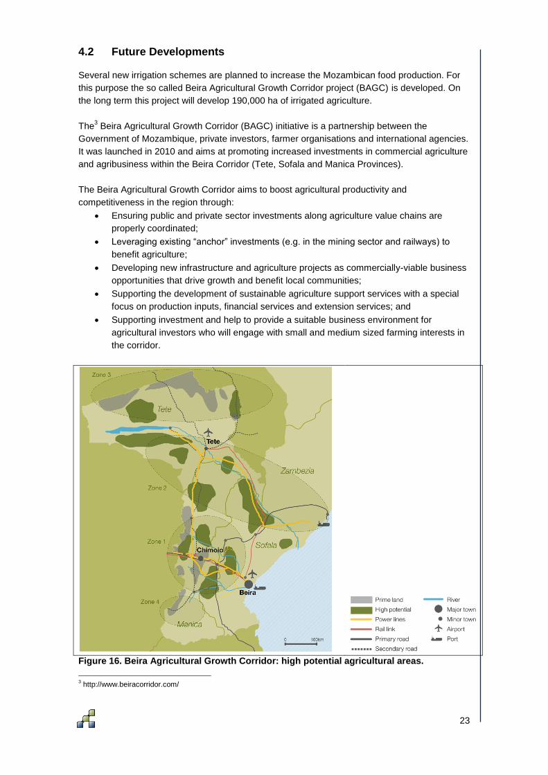
4.2 Future Developments

Several new irrigation schemes are planned to increase the Mozambican food production. For

this purpose the so called Beira Agricultural Growth Corridor project (BAGC) is developed. On

the long term this project will develop 190,000 ha of irrigated agriculture.

The3 Beira Agricultural Growth Corridor (BAGC) initiative is a partnership between the

Government of Mozambique, private investors, farmer organisations and international agencies.

It was launched in 2010 and aims at promoting increased investments in commercial agriculture

and agribusiness within the Beira Corridor (Tete, Sofala and Manica Provinces).

The Beira Agricultural Growth Corridor aims to boost agricultural productivity and

competitiveness in the region through:

Ensuring public and private sector investments along agriculture value chains are

properly coordinated;

Leveraging existing “anchor” investments (e.g. in the mining sector and railways) to

benefit agriculture;

Developing new infrastructure and agriculture projects as commercially-viable business

opportunities that drive growth and benefit local communities;

Supporting the development of sustainable agriculture support services with a special

focus on production inputs, financial services and extension services; and

Supporting investment and help to provide a suitable business environment for

agricultural investors who will engage with small and medium sized farming interests in

the corridor.

Figure 16. Beira Agricultural Growth Corridor: high potential agricultural areas.

3 http://www.beiracorridor.com/

24

In this modeling pilot study a full analysis of water demands, supply and shortages as a result of

the BAGC irrigation component is not foreseen. However, a first order estimate of the potential

water related challenges the BAGC will face, has been made using the WEAP model. For this it

was assumed that irrigated agriculture will be developed around Chimoio. Water for this

irrigation is assumed to originate from both the main Pungwe as well as from the Vunduzi.

Three scenarios are analyzed here to explore the impact of an extension of irrigation:

#1: Extent of 5,000 ha

#2: Extent of 10,000 ha

#3: Extent of 25,000 ha

00_Reference

01_BAGC

02_BAGC

03_BAGC

Water Demand (not including loss, reuse and DSM)

Monthly Average

January March April May June July August October December

Million C

ubic

Mete

r

110

100

90

80

70

60

50

40

30

20

10

0

Figure 17. Monthly average water demand under the three scenarios.

A summary of these findings is presented here, while the various Figures provide more detail:

Total annual average water demand will increase from 550 MCM (currently) to 600

MCM (#1), 650 MCM (#2), and 800 MCM (#3). This increase in water demand is well

distributed over the year. (Figure 17)

The water shortage (unmet demand) used to be small with about 15 MCM/yr currently.

The expansion of irrigation will lead to an average annual water shortage of about 25

MCM (#1), 35 MCM (#2), and 100 MCM (#3). (Figure 18)

Combining this demand with the unmet demand provides the coverage of water.

Focusing on the new BACG irrigated areas this coverage varies per month and for the

driest month (August) this can be as low as 50% for the largest expansion (#3). Figure

19 provides averages over 10 years. Considering the individual 120 months in those ten

years during quite some months even a coverage of 50% cannot be met:

o #1: 9 months (out of 120)

o #2: 16 months (out of 120)

o #3: 23 months (out of 120)

The impact of these new irrigation developments on outflow from Pungwe River into the

Indian Ocean is also analyzed. Especially during the low flow periods (May-Nov) decreases

25

in flows of 10 m3 s

-1 can be expected for the scenario #3. Actual flows will therefore fall

below the critical level of 10 m3 s

-1 frequently. For the other two scenarios decreases in

flows are relatively small.

00_Reference

01_BAGC

02_BAGC

03_BAGC

Unmet Demand

All Demand Sites (27), Monthly Average

January March April May June July August October December

Million C

ubic

Mete

r

24

22

20

18

16

14

12

10

8

6

4

2

0

Figure 18. Monthly average water shortage (unmet demand) under the three scenarios.

00_Reference

01_BAGC

02_BAGC

03_BAGC

Demand Site Coverage (% of requirement met)

Demand Site: BAGC, Monthly Average

January February March April May June July August October December

Perc

ent

100

95

90

85

80

75

70

65

60

55

50

45

40

35

30

25

20

15

10

5

0

Figure 19. Coverage of water demand under the three scenarios.

26

00_Reference

01_BAGC

02_BAGC

03_BAGC

Streamflow (below node or reach listed)

Pungue Nodes and Reaches: Below MinFlowReq, Monthly Average, River: Pungue

January February March April May June July August October December

Cubic

Mete

rs p

er

Seco

nd

0.0

-0.5

-1.0

-1.5

-2.0

-2.5

-3.0

-3.5

-4.0

-4.5

-5.0

-5.5

-6.0

-6.5

-7.0

-7.5

-8.0

-8.5

-9.0

-9.5

Figure 20. Impact of the three BAGC scenarios on outflows of the Pungwe. The Graph

shows the reduction in flows compared to the reference condition.

4.3 Water Infrastructure Developments

It is clear that development of new irrigation schemes without any other developments will

increase water shortages in the basin to undesirable levels. If irrigation expansion is limited to

10,000 ha no severe problems can be expected. Larger expansions can only be justified if

additional measures are taken. Typical examples of measures are: changes in agricultural water

management practices, changes in cropping patters, additional water sources (e.g.

groundwater, interbasin transfer), water savings in other sectors, amongst others. For this pilot

project the option to develop small scale reservoirs have been analyzed.

The effectiveness of these small scale reservoirs is analyzed for the scenario of an extent of

irrigated area by 25,000 ha. Three options of reservoir capacity are explored:

Res_01: storage capacity of 25 Million Cubic Meters

Res_02: storage capacity of 50 Million Cubic Meters

Res_03: storage capacity of 100 Million Cubic Meters

Translating this in practical terms, using the 25 MCM as example, means that for every hectare

irrigation 1000 m3 storage should be created. If a reservoirs is on average 5 m deep, 2% of the

area should be covered by reservoirs (= 200 m2 per hectare). It might be interesting to explore

whether a combination with some medium-scale or large-scale reservoirs is feasible. Also,

combining reservoirs with groundwater storage, by enhancing surface infiltration, might be an

option.

The results of implementing one of these three storage capacities can be summarized as

follows:

27

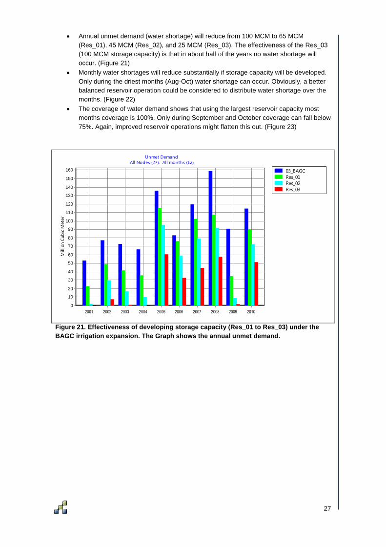
Annual unmet demand (water shortage) will reduce from 100 MCM to 65 MCM

(Res_01), 45 MCM (Res_02), and 25 MCM (Res_03). The effectiveness of the Res_03

(100 MCM storage capacity) is that in about half of the years no water shortage will

occur. (Figure 21)

Monthly water shortages will reduce substantially if storage capacity will be developed.

Only during the driest months (Aug-Oct) water shortage can occur. Obviously, a better

balanced reservoir operation could be considered to distribute water shortage over the

months. (Figure 22)

The coverage of water demand shows that using the largest reservoir capacity most

months coverage is 100%. Only during September and October coverage can fall below

75%. Again, improved reservoir operations might flatten this out. (Figure 23)

03_BAGC

Res_01

Res_02

Res_03

Unmet Demand

All Nodes (27), All months (12)

2001 2002 2003 2004 2005 2006 2007 2008 2009 2010

Million C

ubic

Mete

r

160

150

140

130

120

110

100

90

80

70

60

50

40

30

20

10

0

Figure 21. Effectiveness of developing storage capacity (Res_01 to Res_03) under the

BAGC irrigation expansion. The Graph shows the annual unmet demand.

28

03_BAGC

Res_01

Res_02

Res_03

Unmet Demand

All Nodes (27), Monthly Average

January March April May June July August October December

Million C

ubic

Mete

r

24

22

20

18

16

14

12

10

8

6

4

2

0

Figure 22. Effectiveness of developing storage capacity (Res_01 to Res_03) under the

BAGC irrigation expansion. The Graph shows the average annual unmet demand over a

period of 10 years.

03_BAGC

Res_01

Res_02

Res_03

Demand Site Coverage (% of requirement met)

Demand Site: BAGC, Monthly Average

January February March April May June July August October December

Perc

ent

100

95

90

85

80

75

70

65

60

55

50

45

40

35

30

25

20

15

10

5

0

Figure 23. Effectiveness of developing storage capacity (Res_01 to Res_03) under the

BAGC irrigation expansion. The Graph shows the coverage of water demand.

29

4.4 Daily Reservoir Operations

WEAP was originally developed as a strategic decision support system (S-DSS). Over the last

years, WEAP has been further developed to be used as an operational decision support system

(O-DSS) for water managers. WEAP does not include the full hydraulic processes as other O-

DSS such as SOBEK, HEC-RAS, MIKE-11, amongst others, but has particular strengths in

operational management of water allocation. Since WEAP is based on a simplified hydraulic

representation and not on the full hydraulic processes, data requirements are much lower and

usability is relatively easy.

Within WEAP a diverse set of operational rules for reservoir management exists. WEAP can

therefore function as an operational decision support system (O-DSS) to explore decisions on

the impact on water delivery, shortages and reservoir status. From the existing options the

following two reservoir operational rules were explored here:

Top of Buffer: A reservoir releases water from the conservation pool to fully meet

withdrawal and other downstream requirements, and demand for energy from

hydropower. Once the storage level drops into the buffer pool, the release will be

restricted according to the buffer coefficient, to conserve the reservoir's dwindling

supplies.

Buffer Coefficient: The buffer coefficient is the fraction of the water in the buffer zone

available each day for release. Thus, a coefficient close to 1.0 will cause demands to be

met more fully while rapidly emptying the buffer zone, while a coefficient close to 0 will

leave demands unmet while preserving the storage in the buffer zone.

To demonstrate the use of WEAP in an operational mode, the proposed option to construct a

reservoir about 150 km upstream from Beira, is explored. The existing WEAP model as

described in the previous sections has been changed. The most important changes are:

Streamflow is not assessed using the catchment approach, but observed streamflow

from station E651 has been used

The model was setup at a daily time-step

Only the water demand downstream of the proposed reservoir has been evaluated.

A screenshot of the model developed can be seen in Figure 24. The model was setup using

streamflow data from station E651. In reality observed streamflow data does not exist for the

future, but can be projected using WEAP by including forecasted weather data. At the beginning

of the dry period water managers are then confronted with decisions on when and how much

water from the reservoir should be released on a particular day. This is a repetitive decision

process, either daily or weekly, in which WEAP can play a supportive role.

In this particular example we assume that it is the start of the dry season (July) and water

managers make their first round of decisions on the operation of the reservoir. It is assumed

that water managers consider a set of water conservation operations and would like to know the

impact on releases and reservoir storage over the dry period. In Table 5 a total of five possible

operations are shown, but other ones can be easily evaluated as well.

The resulting reservoir volumes and inflows and outflows are shown in Figure 25 and Figure 26.

It is clear that if no conservation would be applied, the reservoir will be emptied quickly and

during prolonged periods no water can be released. Obviously, this will result in undesirable

situations by leaving the city of Beira without a single drop of water. The conservation options

30

can resolve this problem and for a relatively wet year medium conservation is sufficient, while

for a dry year substantial conservation is needed.

The above example shows that reservoir operations can benefit from using WEAP as an

operational decision support system (O-DSS). Water managers will be able to undertake these

analyses on a regular base (daily and/or weekly) to support their decision making.

Table 5. Reservoir operational rules as explored using WEAP as an O-DSS (Operational

Decision Support System).

Top of Buffer Buffer

Coefficient

Reference: no conservation 0%

A: late and low conservation 50% 0.10

B: late and medium conservation 50% 0.05

C: late and strong conservation 50% 0.01

D: early conservation 80% 0.01

Figure 24. The WEAP model used as an O-DSS (Operational Decision Support System) to

explore operational rules for a proposed reservoir.

31

A_Res

B_Res

C_Res

D_Res

Reference

Reservoir Storage Volume

Reservoir: Reservoir_01, Selected days (124/365)

01-Ju

l-05

08-Ju

l-05

16-Ju

l-05

24-Ju

l-05

01-Au

g-05

09-Au

g-05

17-Au

g-05

25-Au

g-05

02-Se

p-05

10-Se

p-05

18-Se

p-05

26-Se

p-05

05-Oc

t-05

14-Oc

t-05

23-Oc

t-05

01-No

v -05

Million C

ubic

Mete

r24

22

20

18

16

14

12

10

8

6

4

2

0

A_Res

B_Res

C_Res

D_Res

Reference

Reservoir Storage Volume

Reservoir: Reservoir_01, Selected days (124/365)

01-Ju

l-06

08-Ju

l-06

16-Ju

l-06

24-Ju

l-06

01-Au

g-06

09-Au

g-06

17-Au

g-06

25-Au

g-06

02-Se

p-06

10-Se

p-06

18-Se

p-06

26-Se

p-06

05-Oc

t-06

14-Oc

t-06

23-Oc

t-06

01-No

v -06

Million C

ubic

Mete

r

24

22

20

18

16

14

12

10

8

6

4

2

0

Figure 25. Different operations of the reservoir and its impact on reservoir volume as

explored using WEAP as an O-DSS (Operational Decision Support System). Data used

for two historic years 2005 (top) and 2006 (bottom) as demonstration.

32

Decrease in Storage for Reservoir_01

Increase in Storage for Reservoir_01

Inflow from Upstream

Net Evaporation

Outflow to Downstream

Reservoir Inflows and Outflows

Scenario: D_Res, Selected days (124/365), All Reservoirs (1)

01-Ju

l-05

10-Ju

l-05

20-Ju

l-05

30-Ju

l-05

09-Au

g-05

19-Au

g-05

29-Au

g-05

08-Se

p-05

18-Se

p-05

29-Se

p-05

10-Oc

t-05

21-Oc

t-05

01-No

v -05

Million C

ubic

Mete

r6.0

5.0

4.0

3.0

2.0

1.0

0.0

-1.0

-2.0

-3.0

-4.0

-5.0

Figure 26. Reservoir inflows and outflows for the management scenario “early

conservation” as explored using WEAP as an O-DSS (Operational Decision Support

System). Data used from a historic year (2005) as demonstration.

33

5 Conclusions and Recommendations

Mozambique’s development pathways require a proper water governance system. An important

aspect in this regard is knowledge on current and future water challenges. In the pilot study as

described in this report, a water allocation model, based on the WEAP framework, has been

developed. As pilot area the Pungwe River basin in central Mozambique has been used, which

is under management of ARA-Centro.

The most important conclusions from this study can be summarized as:

Current water shortages in the Pungwe Basin are relatively low. The biggest problem is

low flow conditions during the dry period which lead to salt intrusion and therefore

saline water intake by Mafabisse and FIPAG.

An increase in water abstractions can alter the system in a way that water shortage will

become a large problem with negative consequences on people and economy. As long

as development in irrigation is limited to about 10,000 hectare impact will be relatively

modest. A further expansion of water demands, either by irrigation or other sectors, will

lead to severe water shortages if no appropriate actions are taken.

The option to retain water in small-scale reservoirs has been evaluated using the water

allocation model developed during this pilot study. If 25,000 hectare irrigation would be

developed, storage capacity of about 100 million cubic meter of water is needed.

Obviously other water saving options could be considered as well.

The most relevant recommendations for further activities are:

The model as developed in this study can be improved using updated datasets and

information. More extensive use of remote sensing combined with data collected on the

ground will improve model reliability even further.

A further analysis on the impact of the Beira Agricultural Growth Corridor project on

water resources is needed. Focus should be on impact and by a more rigorous analysis

of effectiveness of mitigation measures.

34

6 Selected References

Beira Agricultural Growth Corridor (BAGC). 2014. http://www.beiracorridor.com/

Chamuço, A.L., 1997, Bue Maria dam, Mozambique; multipurpose reservoir operation using

genetic algorithm techniques. MSc Thesis. IHE, Delft

Chamuço, A.L., 1997, Bue Maria dam, Mozambique; multipurpose reservoir operation using

genetic algorithm techniques. MSc Thesis. IHE, Delft

GRM, GRZ. 2007. A monograph of the Pungwe River Basin. Government of the Republic of

Mozambique (GRM) and Government of the Republic of Zimbabwe (GRZ).

Pungwe Project. 2006. http://www.elmed-rostov.ru/Projects/Pungwe%20CD/INDEX.htm

SWECO. 2004. Development of the Pungwe River Basin joint IWRM strategy. Monograph

Report Annex I: Surface Water Resources.

Terink. 2014. Hydrological analysis and modelling of the Pungwe River Basin, Mozambique.

Report FutureWater 126.

Zaag, P van der. 2000. The Pungwe River Basin. UNESCO-IHE, Delft

Zanting, H.A., C. Nacueve & B. Novela, 1994, Salt intrusion in the Pungue estuary. DNA,

Maputo / Companhia de Aguas da Beira E.E., Beira; p.1-3; p.19, p.29-32

Zanting, H.A., C. Nacueve & B. Novela, 1994, Salt intrusion in the Pungue estuary.

DNA,Maputo / Companhia de Aguas da Beira E.E., Beira; p.1-3; p.19, p.29-32