Watch and Learn: Semi-Supervised Learning of Object Detectors from Videos

Ishan Misra Abhinav Shrivastava Martial Hebert

Robotics Institute, Carnegie Mellon University

{imisra,ashrivas,hebert}@cs.cmu.edu

Abstract

We present a semi-supervised approach that localizes

multiple unknown object instances in long videos. We start

with a handful of labeled boxes and iteratively learn and

label hundreds of thousands of object instances. We pro-

pose criteria for reliable object detection and tracking for

constraining the semi-supervised learning process and min-

imizing semantic drift. Our approach does not assume

exhaustive labeling of each object instance in any single

frame, or any explicit annotation of negative data. Working

in such a generic setting allow us to tackle multiple object

instances in video, many of which are static. In contrast,

existing approaches either do not consider multiple object

instances per video, or rely heavily on the motion of the

objects present. The experiments demonstrate the effective-

ness of our approach by evaluating the automatically la-

beled data on a variety of metrics like quality, coverage (re-

call), diversity, and relevance to training an object detector.

1. Introduction

The availability of large labeled image datasets [11, 13]

has been one of the key factors for advances in recog-

nition. These datasets, which have been largely curated

from internet images, have not only helped boost perfor-

mance [14, 19], but have also fostered the development of

new techniques [19, 30]. However, compared to images,

videos seem like a more natural source of training data be-

cause of the additional temporal continuity they offer for

both learning and labeling. So ideally we should have large

labeled internet video datasets. In general, the human effort

required for labeling these vision datasets is huge, e.g., Im-

ageNet [11] required 19 man-years to label bounding boxes

in the 1.2 million images harvested from the internet. Con-

sider the scale of internet videos – YouTube has 100 hours

of video (10 million frames) uploaded every minute. It

seems unlikely that human per-image labeling will scale to

this amount of data. Given this scale of data and the asso-

ciated annotation problems [39, 55], which are more pro-

nounced in videos, it is no surprise that richly annotated

Sparse labeled examples Unlabeled Videos

Learn

Learned Examples Automatically labeled examples

Watch

Label

Figure 1: We present a novel formulation of semi-

supervised learning for automatically learning object de-

tectors from videos. Our method works with long video

to automatically learn bounding box level annotations for

multiple object instances. It does not assume exhaustive la-

beling of every object instance in the input videos, and from

a handful of labeled instances can automatically label hun-

dreds of thousands of instances.

large video recognition datasets are hard to find. In fact, the

available video datasets [28, 29, 37, 39] lack the kind of an-

notations offered by benchmark image datasets [11, 13, 34].

One way to tackle the labeling problem is using semi-

supervised learning (SSL). Starting with only a few anno-

tated examples, the algorithm can label more examples au-

tomatically. However, a major challenge for any kind of

SSL technique is to constrain the learning process to avoid

semantic drift, i.e., added noisy samples cause the learner to

drift away from the true concept. Recent work [7, 8, 12, 46]

has shown ways to constrain this learning process for im-

ages. In this paper, we present an approach to constrain the

semi-supervised learning process [46] in videos. Our tech-

nique constrains the SSL process by using multiple weak

cues - appearance, motion, temporal etc., in video data and

automatically learns diverse new examples.

Intuitively, algorithms dealing with videos should use

appearance and temporal cues using detection and track-

ing, respectively. One would expect a simple combination

of detection and tracking to constitute a semi-supervised

1

framework that would prevent drift since both of these pro-

cesses would ideally cancel each others’ errors. However,

as we show in our experiments (Sec. 5), a naıve combina-

tion of these two techniques performs poorly. In the long

run, the errors in both detection and tracking are ampli-

fied in a coupled system. We can also consider pure detec-

tion approaches or pure tracking approaches for this prob-

lem. However, pure detection ignores temporal information

while pure tracking tends to stray away over a long duration.

We present a scalable framework that discovers objects

in video using SSL (see Figure 1). It tackles the challenging

problem of localizing new object instances in long videos

starting from only a few labeled examples. In addition, we

present our algorithm in a realistic setting of “sparse la-

bels” [39], i.e., in the few initial “labeled” frames, not all

objects are annotated. This setting relaxes the assumption

that in a given frame, all object instances have been exhaus-

tively annotated. It implies that we do not know if any unan-

notated region in the frame belongs to the object category

or the background, and thus cannot use any region from our

input as negative data. While much of the past work has ig-

nored this type of sparse labeling (and lack of explicit neg-

atives), we show ways to overcome this handicap. Figure 2

presents an overview of our algorithm. Our proposed algo-

rithm is different from the rich body of work on tracking-by-

detection. Firstly, we do not attempt to solve the problem

of data association. Our framework does not try to identify

whether it has seen a particular instance before. Secondly,

since it works in the regime of sparse annotations, it does

not assume that negative data can be sampled from around

the current box. Thirdly, we limit expensive computation to

a subset of the input frames to scale to a million frames.

Contributions: We present a semi-supervised learning

framework that localizes multiple unknown objects in

videos. Starting from few sparsely labeled objects, it itera-

tively labels new and useful training examples in the videos.

Our key contributions are: 1) We tackle the SSL problem

for discovering multiple objects in sparsely labeled videos;

2) We present an approach to constrain SSL by combin-

ing multiple weak cues in videos and exploiting decorre-

lated errors by modeling data in multiple feature spaces.

We demonstrate its effectiveness as compared to traditional

tracking-by-detection approaches; 3) Given the redundancy

in video data, we need a method that can automatically de-

termine the relevance of training examples to the target de-

tection task. We present a way to include relevance and

diversity of the training examples in each iteration of the

SSL process, leading to a scalable incremental learning al-

gorithm.

2. Related Work

The availability of web scale image and video data

has made semi-supervised learning more popular in recent

years. In the case of images, many methods [9, 15] rely

on image similarity measures, and try to assign similar la-

bels to close-by unlabeled images. However, in the case

of real-world images, obtaining good image similarity is

hard and hence the simple approaches become less appli-

cable. One major body of work [7, 8, 12, 31, 46] tries to

overcome this difficulty by leveraging the use of a set of

pre-defined attributes for image classes [8, 46] and addition-

ally web-supervision and text [7, 12]. While these methods

have good performance for images, they are not applicable

to videos mainly because they treat each image indepen-

dently and do not use video constraints. One major reason

for the success of attribute based methods for SSL was the

relatively cheap supervision required for attributes (per im-

age level tag). In the same spirit, weakly supervised video

approaches use tags available with internet videos.

Weakly supervised video algorithms have gained popu-

larity largely due to the abundance of video level tags on

the internet. The input is a set of videos with video level

tags (generally a video belongs to an object category), and

the algorithm discovers the object (if present) in the video.

These methods, while effective, assume a maximum of one

dominant object per video [35, 42, 49, 53]. Some of them

additionally assume dominant motion [42] or appearance

saliency [32, 35, 42, 49, 53] for the object of interest. The

methods of video co-segmentation [6, 16, 21, 25] can be

considered a subset of weakly supervised methods. They

make a strong assumption that multiple videos contain the

exact same object in majority of the frames. This assump-

tion of at most one salient object in a video is rarely sat-

isfied by internet or real world videos. When this assump-

tion does not hold, methods cannot strongly rely on mo-

tion based foreground/background clustering or on appear-

ance saliency. Our proposed work deals with multiple ob-

jects and can even discover static object instances without

strongly relying on motion/appearance saliency. However,

we do require richer bounding box annotations by way of

a few sparsely labeled instances. A concurrent work [33]

utilizes weakly labeled video for improving detection.

A relevant thread of work which also uses bounding box

annotations is that of tracking-by-detection. It has a long

and rich history in computer vision and the reader is re-

ferred to [40] for a survey. The tracking-by-detection algo-

rithms start with bounding box annotation(s) of the object(s)

to track the object(s) over a long period of time. The under-

lying assumption is that negative data can be sampled from

around the object [2, 20, 22, 26, 44, 48, 50] to distinguish

between the object and background. This is not valid in the

case of sparsely labeled videos because the unmarked re-

gions may contain more instances of the same object, rather

than background.

Other tracking-by-detection methods [3, 17, 41] do not

sample negative data from the input video. They do so at

the cost of using a detector trained on additional training

Fea

ture

1

Feature 2

(a) Sparse labeled frames

(b) Unlabeled videos (c) Decorrelated Errors

(d) Reliable Tracking (e) New labeled examples (f) Selected Positives

Object

detection Object

Detectors

Figure 2: Our approach selects samples by iteratively discovering new boxes by a careful fusion of detection, robust tracking,

relocalization and multi-view modeling of positive data. It shows how an interplay between these techniques can be used to

learn from large scale unlabeled video corpora.

data, e.g., [41] uses a DPM [14] trained on images from

PASCAL [13]. In contrast, we do not use such additional

training data for our method. This allows us to work on

object categories which are not in standard datasets.

Multi-object tracking-by-detection approaches also fo-

cus on solving the problem of data association - given ob-

ject locations across multiple frames, determine which loca-

tions belong to the same object. Data association is critical

for long term tracking, and is also very challenging [3]. In

contrast, our goal is not to track over long periods, but to

get short and reliable tracking. Moreover, we do not require

these short tracklets to be associated with each other, and

thus have minimal need for data association.

To summarize, our SSL framework operates in a less re-

strictive domain compared to existing work in weakly la-

beled object discovery and tracking-by-detection. The key

differences are: 1) We localize multiple objects in a single

frame as opposed to zero or one objects. 2) We do not as-

sume strong motion or appearance saliency of objects, thus

discovering static object instances as well. 3) We operate in

the regime of sparsely labeled videos. Thus, in any given

frame, all the unmarked region may contain instances of the

object. This does not allow using negative data from the

input frame. 4) We do not need explicit negative data or

any pre-trained object models. 5) Finally, the aim of our

approach is very different from tracking approaches. We

do not want to track objects over a long period of time, but

want short reliable tracklets.

3. Approach OverviewThere are two ways to detect objects in videos – ei-

ther using detection in individual frames or tracking across

frames. In a semi-supervised framework, detection plays

the role of constraining the system by providing an appear-

ance prior for the object, while tracking generalizes by pro-

viding newer views of the object. So one could imagine

a detection and tracking combination, in which one tracks

from confident detections and then updates the detector us-

ing the tracked samples. However, as we show in our exper-

iments (Section 5), such a naıve combination does not im-

Figure 3: Sparsely labeled positives (as shown in the top

row) are used to train Exemplar detectors [36]. Since we do

not assume exhaustive labeling of each instance in the im-

age, we cannot sample negative data from around the input

boxes. When these detectors (trained without domain nega-

tives) are used, they may learn background features (like the

co-occuring yellow stripes or road divider) and give high

confidence false positives (bottom row). We address this

issue by exploiting decorrelated errors (Section 4.1)

pose enough constraints for SSL. In contrast, our approach

builds on top of this basic combination of detection and

tracking to correct their mistakes.

Our algorithm starts with a few sparsely annotated video

frames (L) and iteratively discovers new instances in the

large unlabeled set of videos (U ). Simply put, we first train

detectors on annotated objects, followed by detection on in-

put videos. We determine good detections (removing confi-

dent false positives) which serve as starting points for short-

term tracking. The short-term tracking aims to label new

and unseen examples reliably. Amongst these newly labeled

examples, we identify good and diverse examples which are

used to update the detector without re-training from scratch.

We iteratively repeat this fusion of tracking and detection to

label new examples. We now describe our algorithm (illus-

trated in Figure 2).

Sparse Annotations (lack of explicit negatives): We start

with a few sparsely annotated frames in a random sub-

set of U . Sparse labeling implies that unlike other ap-

proaches [26], we do not assume exhaustively annotated

input, and thus cannot sample negatives from the vicinity

of labeled positives. We use random images from the in-

ternet as negative data for training object detectors on these

sparse labels [45]. We use these detectors to detect objects

on a subset of the video, e.g., every 30 frames. Training on

a few positives without domain negatives can result in high

confidence false positives as shown in Figure 3. Removing

such false positives is important because if we track them,

we will add more bad training examples, thus degrading the

detector’s performance over iterations.

Temporally consistent detections: We first remove detec-

tions that are temporally inconsistent using a smoothness

prior on the motion of detections.

Decorrelated errors: To remove high confidence false pos-

itives (see Figure 3), we rely on the principle of decorre-

lated errors (similar to multi-view SSL [43, 47]). The intu-

ition is that the detector makes mistakes that are related to

its feature representation [52], and a different feature repre-

sentation would lead to different errors. Thus, if the errors

in different feature spaces are decorrelated, one can correct

them and remove false positives. This gives us a filtered set

of detections.

Reliable tracking: We track these filtered detections to la-

bel new examples. Our final goal is not to track the object

over a long period. Instead, our goal is to track reliably and

label new and hopefully diverse examples for the object de-

tector. To get such reliable tracks we design a conservative

short-term tracking algorithm that identifies tracking fail-

ures. Traditional tracking-by-detection approaches [17, 41]

rely heavily on the detection prior to identify tracking fail-

ures. In contrast, the goal of our tracking is to improve

the (weak) detector itself. Thus, heavily relying on input

from the detector defeats the purpose of using tracking in

our case.

Selection of diverse positives for updating the detector:

The reliable tracklets give us a large set of automatically la-

beled boxes which we use to update our detector. Previous

work [42] temporally subsamples boxes from videos, treat-

ing each box with equal importance. However, since these

boxes come from videos, a large number of them are re-

dundant and do not have equal importance for training our

detector. Additionally, the relevance of an example added at

the current iteration i depends on whether similar examples

were added in earlier iterations. One would ideally want to

train (make an incremental update) only on new and diverse

examples, rather than re-train from scratch on thousands of

largely redundant boxes. We address this issue by selec-

tion and show a way of training only on diverse, new boxes.

After training detectors on diverse examples, we repeat the

SSL process to iteratively label more examples.

Stopping criterion of SSL: It is desirable to have SSL al-

gorithms which automatically determine when they should

stop. We stop our SSL once our selection algorithm indi-

cates that it does not have any good candidates to select.

4. Approach DetailsWe start with a small sparsely labeled set L0 of bounding

boxes and unlabeled input videos U . At each iteration i,

using models trained on Li−1, we want to label new boxes

in the input videos U , add them to our labeled set L = L ∪Li, and iteratively repeat this procedure.

4.1. Detections with decorrelated errorsWe train object detectors on our initial set of examples

using random images from Flickr as negatives [45]. We

detect on a uniformly sampled subset of the video frames

and remove the temporally inconsistent detections.

Since the negative data for training the detectors comes

from a different domain than the positives, we still get con-

sistent false positive detections because the detector learns

the wrong concept (see Figures 3 and 5). To remove

such false positives, we perform outlier removal in a fea-

ture space different from that of the detector. The intuition

is that the errors made by learning methods are correlated

with their underlying feature representation, and thus using

decorrelated feature spaces might help correct them.

For outlier removal, we use unconstrained Least Squares

Importance Fitting (uLSIF) [27]. uLSIF uses definite inliers

(our labeled set Li−1) to identify outliers in unknown data.

It scales well with the size of the input and can be com-

puted in closed form. These final filtered detections serve

as starting points for reliable short term tracking.

4.2. Reliable Tracking

We formulate a scalable tracking procedure that ef-

fectively capitalizes on priors available from detection,

color/texture consistency, objectness [1, 51] and optical

flow. More importantly, our tracking procedure is very good

at identifying its own failures. This property is vital in our

semi-supervised framework since any tracking failure will

add wrong examples to the labeled set leading to quick se-

mantic drift (see Figure 5). The short-term tracking pro-

duces a set of labeled examples Li.

Our single object tracking computes sparse optical flow

using Pyramidal Lucas Kanade [5] on Harris feature points.

Since we start with a small set of labeled examples, and do

not perform expensive per-frame detection, our detection

prior is weak. To prevent tracking drift in such cases we

incorporate color/texture consistency by using object pro-

posal bounding boxes [51] obtained from a region around

the tracked box. We address two failure modes of tracking:

Drift due to spurious motion: This occurs while com-

puting optical flow on feature points which are not on the

object, e.g., points on a moving background or occlusion.

To correct this, we first divide each tracked box into four

quadrants and compute the mean flow in each quadrant. We

weigh points in each quadrant by their agreement with the

flow in the other quadrants. The final dominant motion di-

rection for the box is the weighted mean of the flow for

each point. This simple and efficient scheme helps correct

the different motion of feature points not on the object.

Drift due to appearance change: This is incorporated by

object detection boxes and object proposal bounding boxes

in the trellis graph formulation described below.

We formulate the tracking problem as finding the min-

cost path in a graph G. At each frame we incorporate

priors in terms of bounding boxes, i.e., detection bound-

ing boxes, tracked boxes and object proposal bounding

boxes. These boxes are the nodes in our graph and we

connect nodes in consecutive frames with edges forming a

trellis graph. The edge weights are a linear combination

of the difference in dominant motions of the boxes (de-

scribed above), spatial proximity and area change. Track-

ing through this trellis graph G is the equivalent of finding

the single min-cost path, and is efficiently computed using

Dynamic-Programming [3, 41]. As post-processing, we cut

the path as soon as the total cost exceeds a set threshold.

4.3. Selection algorithm:

After we label thousands of boxes Li for the current it-

eration, we use them for improving our object detectors.

Since video data is highly redundant, we label few di-

verse examples and many redundant ones. Training a cate-

gory detector on these thousands of (redundant) boxes, from

scratch, in every iteration is suboptimal. We prefer an incre-

mental training approach that makes incremental updates to

the detector, i.e., trains only on newly added and diverse ex-

amples rather than everything. This is especially important

to prevent drift because even if we label thousands of wrong

but redundant boxes, our method picks only a few of them.

We find the exemplar detectors [23, 36] suitable for incre-

mental learning as they are trained per bounding box.

For each labeled bounding box in Li, we compute a de-

tection signature [24, 38, 54] using our exemplar detectors.

Boxes where our current set of detectors do not give a high

response correspond to examples which are not explained

well by the existing set of detectors. Training on these boxes

increases the coverage of our detectors. Thus, we compute

similarity in this detection signature space to greedily select

a set of boxes that are neither similar to our current detec-

tors, nor amongst themselves.

More formally, let Li = {l1, . . . , lk} be the set of la-

beled boxes at iteration i and E = ∪i−1

j=0Dj the set of boxes

bn associated with the exemplar detectors from all previous

iterations (0 to i−1). We compute the |Li|×|E| detector re-

sponse matrix R. The entry R(m,n) indicates the response

of the detector associated with box bn on box lm (also called

the detection signature [24]). We row-normalize the matrix

R, and denote the detection signature of box lm by its row

R(m). We initialize the set Di ⊂ Li with all the boxes ljwhich have a low response, i.e., none of the detectors from

0 10 20 30 400

0.1

0.2

0.3

0.4

Iterations →

Av

era

ge

Pu

rity

→

ESVM Average Purity across iterations

5 10 15 20 25 30 35 400

0.1

0.2

0.3

0.4

Iterations →

Re

ca

ll →

ESVM Recall across iterations

Boot

Boot+Sel

Det+Track

O w/o Sel

O w/o Outlier

Ours

Figure 4: We measure the detection performance of the ES-

VMs from each ablation method on our test set by comput-

ing (left) Average Purity and (right) Recall.

the previous iterations are confident about detecting these

boxes (ESVM score of < −0.8 and IOU < 0.4).

We iteratively grow the set Di by adding detectors which

minimize the following objective criterion

t∗ = argmaxlt∈Li

∑

bp∈Di,p 6=t

JSD(R(t)||R(p)) (1)

Di = Di ∪ {lt∗}

This objective function favors boxes that are diverse with

respect to the existing detectors using the Jensen-Shannon

Divergence (JSD) of the detection signatures. At each iter-

ation, we limit the number of boxes selected to 10. When

this selection approach is unable to find new boxes, we con-

clude that we have reached the saturation point of our SSL.

This serves as our stopping criterion.

5. Experiments

Our algorithm has a fair number of components inter-

acting with each other across iterations. It is difficult to

characterize the importance of each component by using the

whole system at once. For such component-wise character-

ization, we divide our experiments in two sets. Our first set

of ablative experiments is on a small subset of videos from

VIRAT [39]. In the second set of experiments, we demon-

strate the scalability of our approach to a million frames

from [39]. We also show the generalization of our method

to a different dataset (KITTI [18]). In both these cases we

evaluate the automatically labeled data in terms of qual-

ity, coverage (recall), diversity and relevance to training an

object detector. We now describe the experimental setup

which is common across all our experiments.

Datasets: Due to limited availability of large video datasets

with bounding box annotations, we picked car as our ob-

ject of interest, and two video datasets with a large number

of cars and related objects like trucks, vans etc. We chose

the VIRAT 2.0 Ground [39] dataset for its large number

of frames, and sparsely annotated bounding boxes over all

the frames. This dataset consists of long hours of surveil-

lance videos (static camera) of roads and parking lots. It

has 329 videos (∼1 million frames, and ∼6.5 million anno-

tated bounding boxes (partial ground truth) of cars. We also

evaluate on videos from the KITTI [18] dataset which were

collected by a camera mounted on a moving car. We use the

set 37 videos (∼12,500 frames) which have partial ground

truth boxes (∼41,000 boxes, small cars are not annotated).

Dataset characteristics: We chose these datasets with very

different characteristics (motion, size of object etc.) to test

the generalization of our method. The VIRAT and KITTI

datasets both consist of outdoor scene videos with a static

and moving camera respectively. The VIRAT dataset cap-

tures surveillance videos of multiple cars in parking lots.

The cars in this dataset are small compared to the frame

size, tightly packed together and viewed from a distance

(thus no drastic perspective effects). The KITTI dataset

on the other hand, consists of videos taken by a vehicle

mounted camera. It has high motion, large objects, and per-

spective effects. Figure 3 shows examples from both the

datasets demonstrating their visual differences.

Detectors: We use the Exemplar-SVM (ESVM) [36] detec-

tors with 5000 random images from Flickr as negatives [45].

Since per frame detection is expensive, we detect once ev-

ery 30th frame for VIRAT, and every 10th frame for KITTI.

We threshold detections at SVM score of −0.75.

Multiple feature spaces for false positive removal:

We use the uLSIF [27] algorithm on Pyramidal HOG

(PHOG) [4] and color histogram (LAB color with 32×16×16 bins) features computed on a resized box of 200 × 300px. We set the kernel bandwidth for uLSIF by computing

the 75th percentile distance between random pairs of points.

Object proposal windows: We obtain 2000 windows per

image using selective search [51].

5.1. Ablative Analysis of each constraint

To tease apart the contributions of each component de-

scribed in Section 3, we design a set of algorithms using

only a subset of the components.

Bootstrapping (Boot): In this vanilla form of SSL, we train

object detectors on the initial labeled set and perform detec-

tion. The confident detections are used as training examples

for the next iteration detectors.

Bootstrapping with Selection (Boot+Sel): This algorithm

builds upon the bootstrapping approach described above.

However, diverse examples are selected (Section 4.3) from

confident detections to train new detectors.

Detection, Tracking and Clustering (Det+Track): In this

algorithm, we use a basic combination of detection and

tracking. We start tracking from the confident ESVM de-

tections to label new examples. We then use WHO (or

ELDA) [23] clustering [38] on these boxes to select train-

ing examples for the new detectors. For clustering, we use

WHO features on labeled boxes after resizing, followed by

k-means. We choose the best k in the range (5, 10).Ours without outlier (O w/o Outlier): This setup uses our

entire algorithm except outlier removal (Section 4.1). It can

roughly be thought of as Detection+Tracking+Selection.

Ours without selection (O w/o Sel): This algorithm uses

our algorithm except selection (Section 4.3). It uses WHO

clustering for selection like Det+Track.

Ours: We use our full algorithm as detailed in Sections 3.

Ablation dataset: For these set of experiments we use an

input set of 25 videos (∼170,000 frames) and a separate

test set of 17 videos (∼105,000 frames) which we fully an-

notated. All algorithms start with the same sparse labels

consisting of only 21 boxes spread across different videos.

We run them iteratively till 30 iterations.

5.1.1 Qualitative Results

Figure 5 shows a random set of boxes labeled by each ab-

lation method (and used to train ESVMs for that method),

along with the initial set of 21 positive examples. We no-

tice that as iterations proceed, the labeling quality (espe-

cially “tightness” of the boxes) for all methods degrades.

More importantly, the other methods like Boot, Det+Track

etc. show semantic drift (Figure 5 columns 2-5 at iteration

20). We also notice the importance of selection, as Ours

w/o Selection loses good localization ability fairly quickly

(Figure 5 column 6 at iterations 10-30). We believe methods

like [10] can be used to further improve the labeling quality.

5.1.2 ESVM Detection performance

For the input videos, we cannot measure labeling purity be-

cause of partial ground truth (refer to supplementary mate-

rial for an approximation of purity). Instead, we measure

the relevance of labeled boxes to detection. We consider

detection performance on the test set as a proxy for good

labeling. We test the ESVMs selected and trained by each

method across iterations on the held out test set. A good la-

beling would result in an increased detection performance.

Figure 4 shows Average Purity vs. Recall across iterations

for the various methods on the test set. We use Average Pu-

rity, which is same as Average Precision [13] but does not

penalize double-detections, since we are more interested in

whether the ESVMs are good detectors individually, rather

than as an ensemble.We consider an instance correctly la-

beled (or pure) if its Intersection-Over-Union (IOU) with

any ground-truth instance is greater than 0.3. Our method

shows a higher purity and recall, pointing towards mean-

ingful labeling and selection of the input data. It also shows

that every component of our method is crucial for getting

good performance. We stop our method at iteration 40 be-

cause of our stopping criterion (Section 4.3). We got a 2point drop in purity from iteration 40 to 45, proving the va-

lidity of our stopping criterion. This is important since our

algorithm would rather saturate than label noisy examples.

5.1.3 Training on all the automatically labeled data

In this section, we evaluate the effectiveness of all our la-

beled data. For each algorithm, we train an LSVM [14]

(only root filters, mixtures and positive latent updates of

DPM [14]) on the data it labeled, and test it on the held-

out test set. Since it is computationally expensive to train

Table 1: Comparison of our method with baselines as explained in Section 5.1. We train an LSVM [14] on all the automati-

cally labeled data and compute its detection performance on a held-out, fully annotated test set (AP for IOU 0.5).

Automatic Labeling (LSVM) Ground Truth

Iteration Boot. Boot.+Sel. Det+Track O w/o Sel O w/o Outlier Ours Pascal LSVM Pascal DPM VIRAT LSVM

10 1.32 9.09 9.09 11.21 7.32 15.3920.89 29.56 41.38

30 1.94 3.03 6.59 10.83 1.41 17.68

Iter

ati

on

s Ours Ours w/o Selection Ours w/o Outlier Boot + Selection Detection + Tracking Bootstrapping

1

Initial Labeled Set

10

20

30

Figure 5: (a) We look at a subset of the bounding boxes used to train ESVMs across iteration. Each row corresponds to an

ablation method. The top row shows the randomly chosen initial positive bounding boxes (same for each method). The other

methods diverge quickly across iterations, thus showing that constraints are very important for maintaining purity.

an LSVM on the thousands of boxes, we subsample the

labeled boxes (5000 boxes in total for each method using

k-means on WHO [23] features). We sample more boxes

from the earlier iterations of each method, because their la-

beling purity decreases across iterations (Figure 4). We use

the same domain independent negatives [45] for all these

LSVMs (left side in Table 1). Table 1 shows the detec-

tion AP performance of all LSVMs (measured at IOU of

0.5 [13]) for the data labeled at iteration 10 and 30. We

see that LSVM trained on our labeled data outperforms all

other LSVMs. Our performance is close to that of an LSVM

trained on the PASCAL VOC 2007 dataset [13]. This vali-

dates the high quality of our automatically labeled data.

We also note that the performance of an LSVM trained

on the ground truth boxes (VIRAT-LSVM) (5000 boxes

from ∼1 million ground truth boxes using the same k-

means as above) achieves twice the performance. The fact

that all LSVMs (except the ones from PASCAL) are trained

with the same domain-independent negatives, indicates that

the lack of domain-negatives is not the major cause of this

limitation. This suggests that automatic labeling has limita-

tions compared to human annotations. On further scrutiny

of the LSVM trained on our automatically labeled data, we

found that the recall saturates after iteration 30. However,

the precision was within a few points of VIRAT-LSVM.

Since we work with only the confident detections/tracklets

in the high precision/low recall regime, this behavior is

not unexpected. This is also important since our algorithm

would rather saturate than label noisy positives.

5.2. Large scale experimentsIn this section, we evaluate the scalability of our algo-

rithm to millions of frames and object instances. We also

test its generalization on two datasets with widely different

characteristics - VIRAT (static camera, small cars tightly

packed) and KITTI (moving camera, high motion, large

cars with perspective effects). We use the Boot and Ours

methods described in Section 5.1. As we described in Sec-

tion 2, most of the existing approaches make additional as-

sumptions that are not applicable in our setting, or do not

have publicly available code. To make a fair comparison

against existing methods, we adapt them to our setting.

Baseline - Dense detection and association (Detect +

Track): This algorithm is inspired by Geiger et al. [17]

which has state-of-the-art results on KITTI. The original al-

gorithm uses per-frame detections, followed by a Kalman

filter and data association. We make two changes - 1) To

have a comparable detector across methods, we do not use

a pre-trained DPM on PASCAL VOC 2007. We substitute

it with the ESVMs we have at the current iteration. 2) We

do not use a Kalman filter and use data association over a

short term (maximum 300 frames). We select positives for

the ESVMs by k-means on WHO features [38].

Baseline - Eigen Functions: We modify the Eigen func-

tions [15] method which was originally designed for image

classification. This method uses distances over manifolds to

label unlabeled data. We use basic detection and short term

tracking to get a set of bounding boxes and use eigen func-

tions to classify them as positive or background. The boxes

from previous iterations on which we trained ESVMs are

used as positives and random images from Flickr [45] as

negative data. We use color histogram (32 × 16 × 16 LAB

space) and PHOG [4] features as input to eigen functions.

Datasets: Our input set consists of 312 videos (∼820,000

frames) from VIRAT. We take a held out test set of 17

videos (∼105,000 frames) which we fully annotated. As in-

put, all algorithms start with the same sparse labels consist-

ing of 43 randomly chosen bounding boxes across different

videos. For the KITTI dataset we use 30 videos (∼10,000

frames) as our input and 7 videos (∼2000 frames) for test-

ing. All algorithms start with the same sparse labeled 25

bounding boxes from different videos.

Qualitative Results: We first present qualitative results in

0 10 20 30 400

0.1

0.2

0.3

0.4

Iterations →

Av

era

ge

Pu

rity

→

ESVM Average Purity across iterations

Boot

Eigen Functions

Detect+Track

Ours

(a) Purity on KITTI

0 10 20 30 400

0.1

0.2

0.3

0.4

Iterations →

Re

ca

ll →

ESVM Recall across iterations

Boot

Eigen Functions

Detect+Track

Ours

(b) Recall on KITTI

5 10 15 200

0.1

0.2

0.3

0.4

0.5

Iterations →

Av

era

ge

Pu

rity

→

ESVM Average Purity across iterations

Boot

Eigen Functions

Detect+Track

Ours

(c) Purity on VIRAT

5 10 15 200

0.1

0.2

0.3

0.4

0.5

Iterations →

Re

ca

ll →

ESVM Recall across iterations

Boot

Eigen Functions

Detect+Track

Ours

(d) Recall on VIRAT

Figure 6: We measure the detection performance of the labeled boxes for our large scale experiments. We test the ESVMs

trained at each iteration on the held out test set and compute Average Purity and Recall. Our method outperforms the baselines

by a significant margin. It maintains purity while substantially increasing recall.

1

2

3

4

30

210

60

240

90

270

120

300

150

330

180 0

(a) Initial boxes

10

20

30

40

50

30

210

60

240

90

270

120

300

150

330

180 0

(b) Bootstrapping

50

100

150

30

210

60

240

90

270

120

300

150

330

180 0

(c) Eigen Functions

50

100

150

200

30

210

60

240

90

270

120

300

150

330

180 0

(d) Detect+Track

50

100

150

200

250

30

210

60

240

90

270

120

300

150

330

180 0

(e) Ours

2000

4000

6000

8000

30

210

60

240

90

270

120

300

150

330

180 0

(f) Ground truth

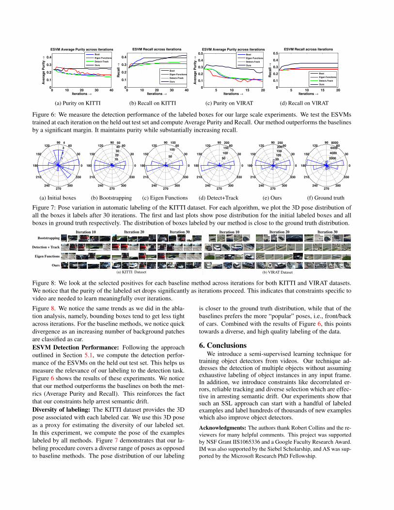
Figure 7: Pose variation in automatic labeling of the KITTI dataset. For each algorithm, we plot the 3D pose distribution of

all the boxes it labels after 30 iterations. The first and last plots show pose distribution for the initial labeled boxes and all

boxes in ground truth respectively. The distribution of boxes labeled by our method is close to the ground truth distribution.

Ours

Bootstrapping

Detection + Track

Eigen Functions

(a) KITTI Dataset (b) VIRAT Dataset

Iteration 20 Iteration 30 Iteration 10 Iteration 10 Iteration 20 Iteration 30

Figure 8: We look at the selected positives for each baseline method across iterations for both KITTI and VIRAT datasets.

We notice that the purity of the labeled set drops significantly as iterations proceed. This indicates that constraints specific to

video are needed to learn meaningfully over iterations.

Figure 8. We notice the same trends as we did in the abla-

tion analysis, namely, bounding boxes tend to get less tight

across iterations. For the baseline methods, we notice quick

divergence as an increasing number of background patches

are classified as car.

ESVM Detection Performance: Following the approach

outlined in Section 5.1, we compute the detection perfor-

mance of the ESVMs on the held out test set. This helps us

measure the relevance of our labeling to the detection task.

Figure 6 shows the results of these experiments. We notice

that our method outperforms the baselines on both the met-

rics (Average Purity and Recall). This reinforces the fact

that our constraints help arrest semantic drift.

Diversity of labeling: The KITTI dataset provides the 3D

pose associated with each labeled car. We use this 3D pose

as a proxy for estimating the diversity of our labeled set.

In this experiment, we compute the pose of the examples

labeled by all methods. Figure 7 demonstrates that our la-

beling procedure covers a diverse range of poses as opposed

to baseline methods. The pose distribution of our labeling

is closer to the ground truth distribution, while that of the

baselines prefers the more “popular” poses, i.e., front/back

of cars. Combined with the results of Figure 6, this points

towards a diverse, and high quality labeling of the data.

6. ConclusionsWe introduce a semi-supervised learning technique for

training object detectors from videos. Our technique ad-dresses the detection of multiple objects without assumingexhaustive labeling of object instances in any input frame.In addition, we introduce constraints like decorrelated er-rors, reliable tracking and diverse selection which are effec-tive in arresting semantic drift. Our experiments show thatsuch an SSL approach can start with a handful of labeledexamples and label hundreds of thousands of new exampleswhich also improve object detectors.

Acknowledgments: The authors thank Robert Collins and the re-

viewers for many helpful comments. This project was supported

by NSF Grant IIS1065336 and a Google Faculty Research Award.

IM was also supported by the Siebel Scholarship, and AS was sup-

ported by the Microsoft Research PhD Fellowship.

References

[1] B. Alexe, T. Deselaers, and V. Ferrari. What is an object? In

CVPR, 2010. 4[2] S. Avidan. Ensemble tracking. In CVPR, 2005. 2[3] J. Berclaz, F. Fleuret, E. Turetken, and P. Fua. Multiple ob-

ject tracking using k-shortest paths optimization. TPAMI,

2011. 2, 3, 5[4] A. Bosch, A. Zisserman, and X. Munoz. Representing shape

with a spatial pyramid kernel. In CVPR, 2007. 6, 7[5] J.-Y. Bouget. Pyramidal implementation of the lucas kanade

feature tracker: Description of the algorithm, 2000. 4[6] D.-J. Chen, H.-T. Chen, and L.-W. Chang. Video object

cosegmentation. In ACM MM, 2012. 2[7] X. Chen, A. Shrivastava, and A. Gupta. NEIL: Extracting

Visual Knowledge from Web Data. In ICCV, 2013. 1, 2[8] J. Choi, M. Rastegari, A. Farhadi, and L. Davis. Adding un-

labeled samples to categories by learned attributes. In CVPR,

2013. 1, 2[9] D. Dai and L. Van Gool. Ensemble projection for semi-

supervised image classification. In ICCV, 2013. 2[10] Q. Dai and D. Hoiem. Learning to localize detected objects.

In CVPR, 2012. 6[11] J. Deng, W. Dong, R. Socher, L. jia Li, K. Li, and L. Fei-

fei. Imagenet: A large-scale hierarchical image database. In

CVPR, 2009. 1[12] S. Divvala, A. Farhadi, and C. Guestrin. Learning everything

about anything: Webly-supervised visual concept learning.

In CVPR, 2014. 1, 2[13] M. Everingham, L. Van Gool, C. K. I. Williams, J. Winn, and

A. Zisserman. The PASCAL Visual Object Classes Chal-

lenge 2007 (VOC2007). 1, 3, 6, 7[14] P. Felzenszwalb, R. Girshick, D. McAllester, and D. Ra-

manan. Object detection with discriminatively trained part-

based models. PAMI, 2010. 1, 3, 6, 7[15] R. Fergus, Y. Weiss, and A. Torralba. Semi-supervised learn-

ing in gigantic image collections. In NIPS, 2009. 2, 7[16] H. Fu, D. Xu, B. Zhang, and S. Lin. Object-based multiple

foreground video co-segmentation. In CVPR, 2014. 2[17] A. Geiger, P. Lenz, C. Stiller, and R. Urtasun. Vision meets

robotics: The kitti dataset. IJRR, 2013. 2, 4, 7[18] A. Geiger, P. Lenz, and R. Urtasun. Are we ready for au-

tonomous driving? the kitti vision benchmark suite. In

CVPR, 2012. 5[19] R. Girshick, J. Donahue, T. Darrell, and J. Malik. Rich fea-

ture hierarchies for accurate object detection and semantic

segmentation. In CVPR, 2014. 1[20] H. Grabner, C. Leistner, and H. Bischof. Semi-supervised

on-line boosting for robust tracking. In ECCV, 2008. 2[21] J. Guo, Z. Li, L.-F. Cheong, and S. Z. Zhou1. Video co-

segmentation for meaningful action extraction. In CVPR,

2013. 2[22] S. Hare, A. Saffari, and P. Torr. Struck: Structured output

tracking with kernels. In ICCV, 2011. 2[23] B. Hariharan, J. Malik, and D. Ramanan. Discriminative

decorrelation for clustering and classification. In ECCV,

2012. 5, 6, 7[24] L. jia Li, H. Su, E. P. Xing, and L. Fei-fei. Object bank:

A high-level image representation for scene classification &

semantic feature sparsification. In NIPS, 2010. 5

[25] A. L. Jose C. Rubio, Joan Serrat. Video cosegmentation. In

ACCV, 2012. 2[26] Z. Kalal, K. Mikolajczyk, and J. Matas. Tracking-learning-

detection. TPAMI, 2012. 2, 3[27] T. Kanamori, S. Hido, and M. Sugiyama. A least-squares

approach to direct importance estimation. JMLR, 2009. 4, 6[28] A. Karpathy, G. Toderici, S. Shetty, T. Leung, R. Sukthankar,

and L. Fei-Fei. Large-scale video classification with convo-

lutional neural networks. In CVPR, 2014. 1[29] A. R. Z. Khurram Soomro and M. Shah. Ucf101: A dataset

of 101 human action classes from videos in the wild. Tech-

nical report, CRCV-TR-12-01, 2012. 1[30] A. Krizhevsky, I. Sutskever, and G. E. Hinton. Imagenet

classification with deep convolutional neural networks. In

NIPS, 2012. 1[31] S. Lad and D. Parikh. Interactively guiding semi-supervised

clustering via attribute-based explanations. In ECCV, 2014.

2[32] Y. J. Lee, J. Ghosh, and K. Grauman. Discovering important

people and objects for egocentric video summarization. In

CVPR, 2012. 2[33] X. Liang, S. Liu, Y. Wei, L. Liu, L. Lin, and S. Yan. Compu-

tational baby learning. arXiv preprint, 2014. 2[34] T.-Y. Lin, M. Maire, S. Belongie, J. Hays, P. Perona, D. Ra-

manan, and C. L. Z. Piotr Dollar. Microsoft coco: Common

objects in context. arXiv, 2014. 1[35] D. Liu, G. Hua, and T. Chen. A hierarchical visual model for

video object summarization. PAMI, 2010. 2[36] T. Malisiewicz, A. Gupta, and A. A. Efros. Ensemble of

exemplar-svms for object detection and beyond. In ICCV,

2011. 3, 5, 6[37] M. Marszałek, I. Laptev, and C. Schmid. Actions in context.

In CVPR, 2009. 1[38] I. Misra, A. Shrivastava, and M. Hebert. Data-driven exem-

plar model selection. In WACV, 2014. 5, 6, 7[39] S. Oh, A. Hoogs, A. Perera, N. Cuntoor, C.-C. Chen, J. T.

Lee, S. Mukherjee, J. K. Aggarwal, H. Lee, L. Davis,

E. Swears, X. Wang, Q. Ji, K. Reddy, M. Shah, C. Vondrick,

H. Pirsiavash, D. Ramanan, J. Yuen, A. Torralba, B. Song,

A. Fong, A. Roy-Chowdhury, and M. Desai. A large-

scale benchmark dataset for event recognition in surveillance

video. In CVPR, 2011. 1, 2, 5[40] Y. Pang and H. Ling. Finding the best from the second bests

- inhibiting subjective bias in evaluation of visual tracking

algorithms. In ICCV, 2013. 2[41] H. Pirsiavash, D. Ramanan, and C. C. Fowlkes. Globally-

optimal greedy algorithms for tracking a variable number of

objects. In CVPR, 2011. 2, 3, 4, 5[42] A. Prest, C. Leistner, J. Civera, C. Schmid, and V. Fer-

rari. Learning object class detectors from weakly annotated

video. In CVPR, 2012. 2, 4[43] C. Rosenberg, M. Hebert, and H. Schneiderman. Semi-

supervised self-training of object detection models. In

WACV, 2005. 4[44] A. Saffari, C. Leistner, M. Godec, and H. Bischof. Robust

multi-view boosting with priors. In ECCV, 2010. 2[45] A. Shrivastava, T. Malisiewicz, A. Gupta, and A. A. Efros.

Data-driven visual similarity for cross-domain image match-

ing. ACM Trans. on Graphics, 2011. 4, 6, 7[46] A. Shrivastava, S. Singh, and A. Gupta. Constrained semi-

supervised learning using attributes and comparative at-

tributes. In ECCV, 2012. 1, 2[47] V. Sindhwani and P. Niyogi. A co-regularized approach

to semi-supervised learning with multiple views. In ICML

Workshop, 2005. 4[48] J. S. Supancic III and D. Ramanan. Self-paced learning for

long-term tracking. In CVPR, 2013. 2[49] K. Tang, R. Sukthankar, J. Yagnik, and L. Fei-Fei. Discrimi-

native segment annotation in weakly labeled video. In CVPR,

2013. 2[50] A. Teichman and S. Thrun. Tracking-based semi-supervised

learning. In RSS, 2011. 2[51] K. E. A. van de Sande, J. R. R. Uijlings, T. Gevers, and

A. W. M. Smeulders. Segmentation as selective search for

object recognition. IJCV, 2011. 4, 6[52] C. Vondrick, A. Khosla, T. Malisiewicz, and A. Torralba.

HOGgles: Visualizing Object Detection Features. ICCV,

2013. 4[53] L. Wang, G. Hua, R. Sukthankar, J. Xue, and N. Zheng.

Video object discovery and co-segmentation with extremely

weak supervision. In ECCV, 2014. 2[54] Y.-X. Wang and M. Hebert. Model recommendation: Gen-

erating object detectors from few samples. In CVPR, 2015.

5[55] J. Yuen, B. C. Russell, C. Liu, and A. Torralba. Labelme

video: Building a video database with human annotations.

In ICCV, 2009. 1