Atmos. Chem. Phys., 16, 15265–15276, 2016www.atmos-chem-phys.net/16/15265/2016/doi:10.5194/acp-16-15265-2016© Author(s) 2016. CC Attribution 3.0 License.

Influence of the Bermuda High on interannual variability ofsummertime ozone in the Houston–Galveston–Brazoria regionYuxuan Wang1,2, Beixi Jia2, Sing-Chun Wang1, Mark Estes3, Lu Shen4, and Yuanyu Xie2

1Department of Earth and Atmospheric Sciences, the University of Houston, Houston, TX, USA2Ministry of Education Key Laboratory for Earth System Modeling, Center for Earth System Science,Tsinghua University, Beijing, China3Texas Commission on Environmental Quality, Austin, TX, USA4School of Engineering and Applied Sciences, Harvard University, Cambridge, MA, USA

Correspondence to: Yuxuan Wang (ywang246@central.uh.edu)

Received: 7 July 2016 – Published in Atmos. Chem. Phys. Discuss.: 12 September 2016Revised: 11 November 2016 – Accepted: 21 November 2016 – Published: 9 December 2016

Abstract. The Bermuda High (BH) quasi-permanent pres-sure system is the key large-scale circulation pattern in-fluencing summertime weather over the eastern and south-ern US. Here we developed a multiple linear regression(MLR) model to characterize the effect of the BH on year-to-year changes in monthly-mean maximum daily 8 h average(MDA8) ozone in the Houston–Galveston–Brazoria (HGB)metropolitan region during June, July, and August (JJA).The BH indicators include the longitude of the BH west-ern edge (BH-Lon) and the BH intensity index (BHI) definedas the pressure gradient along its western edge. Both BH-Lon and BHI are selected by MLR as significant predictors(p < 0.05) of the interannual (1990–2015) variability of theHGB-mean ozone throughout JJA, while local-scale merid-ional wind speed is selected as an additional predictor forAugust only. Local-scale temperature and zonal wind speedare not identified as important factors for any summer month.The best-fit MLR model can explain 61–72 % of the interan-nual variability of the HGB-mean summertime ozone over1990–2015 and shows good performance in cross-validation(R2 higher than 0.48). The BH-Lon is the most importantfactor, which alone explains 38–48 % of such variability. Thelocation and strength of the Bermuda High appears to controlwhether or not low-ozone maritime air from the Gulf of Mex-ico can enter southeastern Texas and affect air quality. Thismechanism also applies to other coastal urban regions alongthe Gulf Coast (e.g., New Orleans, LA, Mobile, AL, and Pen-sacola, FL), suggesting that the BH circulation pattern can

affect surface ozone variability through a large portion of theGulf Coast.

1 Introduction

Surface ozone, as an important air pollutant, has significantadverse impacts on both public health and agriculture. Ozoneis produced in the troposphere by photochemical oxidation ofcarbon monoxide (CO) and volatile organic carbon (VOCs),initiated by reaction with hydroxyl radicals (OH) in the pres-ence of nitrogen oxides (NOx). Surface ozone is influencednot only by emissions of its precursors, but also by meteo-rological conditions (e.g., Jacob and Winner, 2009). Large-scale circulation patterns can lead to local meteorologicalconditions that are favorable for ozone episodes, such ashigh temperatures, low wind speeds, clear skies, and stagna-tion (Nielsen-Gammon et al., 2005a; Ngan and Byun, 2011;Pearce et al., 2011; Psilogloue et al., 2013; Pugliese et al.,2014). Previous studies have demonstrated certain associa-tions between large-scale circulations and surface ozone con-centrations over the US (e.g., Darby, 2005; Rappenglück etal., 2008; Lin et al., 2012, 2015; Zhu and Liang, 2013; Shenet al., 2015). For example, surface ozone in the western USis affected by mid-latitude cyclones that transport Asian pol-lution eastward across the Pacific (Lin et al., 2012) and late-spring stratospheric intrusions occurring more frequently fol-lowing strong La Niña winters (Lin et al., 2015). In the Mid-west and the northeastern US, polar jet frequency is a good

Published by Copernicus Publications on behalf of the European Geosciences Union.

15266 Y. Wang et al.: Influence of the Bermuda High on interannual variability

Figure 1. (a) Locations of the HGB region (blue box). The redboxes show the regions used to define the BH intensity indices BHI;(b) locations of the CAMS sites within the HGB region and thelong-term (1990–2015) mean MDA8 ozone from June to August.

indicator of the interannual variability of surface ozone insummer (Shen et al., 2015).

The Bermuda High (BH), a quasi-permanent system lo-cated over the North Atlantic Ocean (Davis et al., 1997),is the key large-scale circulation pattern that influences theregional climate over the eastern and southern US in sum-mer (Li et al., 2012; Zhu and Liang, 2013; Hegarty et al.,2007; Hogrefe et al., 2004). The BH circulation pattern in-fluences ozone air quality in the US through two mecha-nisms. First, as the BH shifts westward from late spring tosummer, it places the eastern US under high pressures, re-sulting in meteorological conditions favorable for local pro-duction of ozone, such as high temperatures, clear skies, andstagnation. A number of studies have shown that high ozoneconcentrations easily occur over large parts of the northeastunder the BH pressure pattern (Eder et al., 1993; Fiore etal., 2003; Hogrefe et al., 2004). Second, the southerly flowsat the western edge of the BH bring clean marine air fromthe Gulf of Mexico to the southern Great Plains (Higgins etal., 1997). This maritime inflow has lower concentrations ofozone compared with the continental air it replaces, and isthus responsible for low ozone background over much of theGulf States in summer (Langford et al., 2009; Ngan and Byunet al., 2011). These two mechanisms have been illustrated byZhu and Liang (2013). Using observational data, they foundpositive correlations over the northeast between maximumdaily 8 h average (MDA8) surface ozone in summer and theintensity of the BH on the interannual timescale due to thefirst mechanism, but negative correlations over the southern–central US due to the second mechanism. Shen et al. (2015)further suggested that the location of the BH western edgehas an influence on the summer mean MDA8 ozone in thesoutheast.

The Houston–Galveston–Brazoria (HGB) area is a majormetropolitan area on the Gulf Coast located near the west-ern edge of the BH in summer (Fig. 1). The HGB regionwas classified as a “marginal” nonattainment zone for ozone

by the US Environmental Protection Agency (EPA) under the2008 standard (TCEQ, 2012), although mean and peak ozoneof the HGB area has decreased significantly during the pastdecades due to control of anthropogenic emissions (Berlin etal., 2013). A number of studies have demonstrated the im-portance of meteorology and circulation patterns on ozoneover the HGB (Ngan et al., 2011; Rappenglück et al., 2008;Pakalapati et al., 2009; Haman et al., 2014), focusing pre-dominantly on a typical year or episodic high ozone cases,such as those observed during the Texas Air Quality Study-II(Rappenglück et al., 2008; Day et al., 2009). Doppler lidarmeasurements of the strength and direction of the noctur-nal low level jet (LLJ) during the TexAQS 2006 field cam-paign (Tucker et al., 2010) found a relationship between thenocturnal LLJ and ozone concentrations on the next day. Astrong southerly nocturnal LLJ was linked to strong BH con-ditions due to the superposition of the sea breeze cycle on astrong synoptic-scale southerly flow. Given the evidence es-tablished by prior investigations on the overall influence ofthe BH on summertime ozone over the southern US (e.g.,Zhu and Liang, 2013; Shen et al., 2015), we hypothesize thatthe large-scale circulation patterns associated with the BHplay a key role in driving the year-to-year change in surfaceozone over the HGB. In this study we will test this hypothe-sis by examining the statistical relationship between the vari-ability of the BH and MDA8 ozone over the HGB duringJune, July, and August (JJA), a time period when the BH islocated closer to North America and exerts large influenceson circulation patterns over the HGB.

2 Data and methods

2.1 Ozone observations

The HGB region is delineated by longitude from −94.5 to−96.0◦W, and by latitude from 28.5 to 30.5◦ N (blue boxin Fig. 1a). Surface ozone concentrations over the HGBhave been routinely monitored at continuous ambient mon-itoring stations (CAMSs) maintained by the Texas Com-mission on Environmental Quality (TCEQ), the City ofHouston, and Harris County. Observational records of sur-face ozone in JJA from 1990 to 2015 were obtained fromthe EPA AirData website (http://www3.epa.gov/airquality/airdata/ad_data_daily.html). Ozone observations from 28ozone CAMS sites in the HGB region that have data recordslonger than 10 years were used for analysis. Figure 1b dis-plays the site distributions and long-term mean ozone in JJAat each site. The site locations and operation time periodsare provided in Table S1 in the Supplement. The number ofCAMS sites increases to 16 in 1998 and 21 in 2004. Thereare eight sites with continuous observations from 1990 tothe present. The overall data coverage at each selected siteis 99 % during its operation period, except for the HoustonEast site that has ozone observations since 1990 but no data

Atmos. Chem. Phys., 16, 15265–15276, 2016 www.atmos-chem-phys.net/16/15265/2016/

Y. Wang et al.: Influence of the Bermuda High on interannual variability 15267

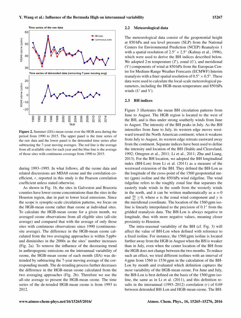
Figure 2. Summer (JJA)-mean ozone over the HGB area during theperiod from 1990 to 2015. The upper panel is the time series ofthe raw data and the lower panel is the detrended time series aftersubtracting the 7-year moving averages. The red line is the averagefrom all available sites for each year and the blue line is the averageof those sites with continuous coverage from 1990 to 2015.

during 1993–1995. In what follows, all the ozone data andrelated discussions are MDA8 ozone and the correlation co-efficient, r , reported in this study is the Pearson correlationcoefficient unless stated otherwise.

As shown in Fig. 1b, the sites in Galveston and Brazoriacounties have lower ozone concentrations than the sites in theHouston region, due in part to lower local emissions. Sincethe scope is synoptic-scale circulation patterns, we focus onthe HGB-mean ozone rather than ozone at individual sites.To calculate the HGB-mean ozone for a given month, weaveraged ozone observations from all eligible sites (all-siteaverage) and compared that with the average of only thosesites with continuous observations since 1990 (continuous-site average). The difference in the HGB-mean ozone cal-culated from the two averaging approaches is within 5 ppbvand diminishes in the 2000s as the sites’ number increases(Fig. 2a). To remove the influence of the decreasing trendin anthropogenic emissions on the interannual variability ofozone, the HGB-mean ozone of each month (JJA) was de-trended by subtracting the 7-year moving average of the cor-responding month. The de-trending process further decreasesthe difference in the HGB-mean ozone calculated from thetwo averaging approaches (Fig. 2b). Therefore we use theall-site average to present the HGB-mean ozone. The timeseries of the de-trended HGB-mean ozone is from 1993 to2012.

2.2 Meteorological data

The meteorological data consist of the geopotential heightat 850 hPa and sea level pressure (SLP) from the NationalCenters for Environmental Prediction (NCEP) Reanalysis 1with a spatial resolution of 2.5◦× 2.5◦ (Kalnay et al., 1996),which were used to derive the BH indices described below.We adopted 2 m temperature (T ), zonal (U ), and meridional(V ) components of wind at 850 hPa from the European Cen-tre for Medium-Range Weather Forecasts (ECMWF) Interimreanalysis with a finer spatial resolution of 0.5◦× 0.5◦. Thesedata were used to calculate the local-scale meteorological pa-rameters, including the HGB-mean temperature and 850 hPawinds (U and V ).

2.3 BH indices

Figure 3 illustrates the mean BH circulation patterns fromJune to August. The HGB region is located to the west ofthe BH, and is thus under strong southerly winds from Juneto August. The intensity of the BH peaks in July. As the BHintensifies from June to July, its western edge moves west-ward toward the North American continent; when it weakensfrom July to August, its western edge retreats eastward awayfrom the continent. Separate indices have been used to definethe intensity and location of the BH (Stahle and Cleaveland,1992; Ortegren et al., 2011; Li et al., 2011; Zhu and Liang,2013). For the BH location, we adopted the BH longitudinalindex (BH-Lon) from Li et al. (2011) as a measure of thewestward extension of the BH. They defined the BH-Lon asthe longitude of the cross-point of the 1560 geopotential me-ter (gpm) isoline and the 850 hPa wind ridgeline. The windridgeline refers to the roughly zonal line that separates theeasterly trade winds in the south from the westerly windsin the north, and it can be written mathematically as u= 0and ∂u

∂y≥ 0, where u is the zonal wind component and y is

the meridional coordinate. The location of the 1560 gpm iso-line is linearly interpolated to the precision of 0.1◦ from thegridded reanalysis data. The BH-Lon is always negative inlongitude, thus with more negative values, meaning closerproximity to Houston.

The intra-seasonal variability of the BH (cf. Fig. 3) willaffect the value of BH-Lon when defined with reference toa fixed isoline. For instance, the 1560 gpm isoline is locatedfurther away from the HGB in August when the BH is weakerthan in July, even when the center location of the BH fromthe HGB does not change between the two months. To reducesuch an effect, we tried different isolines with an interval of4 gpm from 1560 to 1536 gpm in the calculation of the BH-Lon by month and evaluated which definition captures themost variability of the HGB-mean ozone. For June and July,the BH-Lon is best defined on the basis of the 1560 gpm iso-line, the same as in Li et al. (2011), and this definition re-sults in the interannual (1993–2012) correlation (r) of 0.69between detrended BH-Lon and HGB-mean ozone. The BH-

www.atmos-chem-phys.net/16/15265/2016/ Atmos. Chem. Phys., 16, 15265–15276, 2016

15268 Y. Wang et al.: Influence of the Bermuda High on interannual variability

89.8 o W ms-1 ms-1 ms-1 91.9 o W

July

80.0 o W

August June 50º N

40º N

30º N

20º N

120º W 90º W 60º W 30º W

50º N

40º N

30º N

20º N

120º W 90º W 60º W 30º W

50º N

40º N

30º N

20º N

120º W 90º W 60º W 30º W

Figure 3. Distributions of the 1998–2013 mean 850 hPa geopotential height (color contour) and wind fields (arrows; m s−1) in June (left),July (center), and August (right). The thick white dashed line shows the longitude of the BH-Lon (values shown in white).

Figure 4. Time series of the BH-Lon (solid line) in June, July, andAugust from 1990 to 2015. A linear trend (dashed line) is used tofit each time series.

Lon for August is defined using the 1556 gpm and the corre-sponding r is 0.62.

The time series of monthly-mean BH-Lon is shown inFig. 4. In correspondence to the intra-seasonal movement ofthe BH shown in Fig. 3, the mean value of BH-Lon from1990 to 2015 was 80.3◦W in June, 93.1◦W in July, and91.6◦W in August. There were no significant trends in BH-

Lon for the months of June and July. In August, however,BH-Lon exhibited a significant increasing trend (i.e., an east-ward shift) of 0.51◦ a−1 (p < 0.1) over 1990–2015, but thistrend becomes insignificant if the first 4 years (1990–1993)were excluded. Shen et al. (2015) found an increasing trendof 0.35◦ a−1 in the JJA-mean BH-Lon over 1980–2010 us-ing the definition of Li et al. (2011). Rather than a changein the BH circulation patterns, they attributed this trend to aspatially uniform decrease in SLP over the US and the adja-cent Atlantic Ocean in the reanalysis data. Given their workas well as the lack of a consistent trend in the monthly-meanBH-Lon over 1990–2015, we do not consider the trend ofBH-Lon in the present work. To be consistent with the ozonedata, the BH-Lon time series were processed by removingthe 7-year moving averages.

Another type of BH index is defined on the basis ofpressure differences between two representative locations,with their exact locations varying among studies. Zhu andLiang (2013) defined a pressure-based BH index (BHI) as themean SLP difference between a location in the Gulf of Mex-ico and the other in the southern Great Plains where the SLPhas the largest positive and negative correlation with LLJ,respectively. As a result, their BHI exhibits a significant pos-itive association with the strength of LLJ, which determinesthe transport of clean marine air from the Gulf of Mexico.Similar to that study, we defined a pressure-based BHI asthe mean SLP difference along the western edge of the BH,between the same location in the southern Great Plains (35–39◦ N, 105.5–100◦W) as selected by Zhu and Liang (2013)(box 2 in Fig. 1a) and the other in the Gulf of Mexico (25.3–29.3◦ N, 92.5–87.5◦W; box 1 in Fig. 1a) where the SLP ex-hibits the largest correlation with the HGB-mean ozone. OurGulf of Mexico domain is located 2.5◦ east of that defined byZhu and Liang (2013). This BHI shows only weak to mod-erate correlations with BH-Lon, with r being −0.57, −0.26,and −0.39 for JJA, respectively, suggesting the position ofthe BH western edge may not vary coherently with the pres-sure gradient over the western edge. Therefore, both BH-Lonand BHI are used as predictors in the regression model de-scribed below.

Atmos. Chem. Phys., 16, 15265–15276, 2016 www.atmos-chem-phys.net/16/15265/2016/

Y. Wang et al.: Influence of the Bermuda High on interannual variability 15269

Ozo

ne (p

pbv)

Tem

pera

ture

(F)

Figure 5. The 1990–2015 mean monthly MDA8 ozone over theHGB area (black line), overlaid with the average number of ex-ceedance days by month (bars) and the HGB-mean temperature (redline). An exceedance day is defined when MDA8 ozone at one ormore monitors in HGB is higher than 70 ppbv.

2.4 Statistical method

We applied a multiple linear regression (MLR) model, whichhas been commonly used in air quality and meteorologi-cal studies (e.g., Kutner et al., 2004; Tai et al., 2010), toconstruct the statistical relationship between the detrendedHGB-mean ozone and the five meteorological predictors de-scribed above, including BH-Lon, BHI, T , U , and V . Sinceour focus is on variability, all the meteorological predictorswere detrended using the same approach as the ozone data.For ease of comparison, all the meteorological predictorsin the regression analysis were normalized. The regressionwas conducted on the monthly scale from 1993 to 2012. Themodel is of the form

y = β0+∑n

k=1βkχk, (1)

where y is the detrended monthly HGB-mean MDA8 O3, nis the number of predictors, χk represents the kth predictorwhich is detrended and normalized, βk is the correspond-ing regression coefficient for χk , and β0 is the intercept. Thepredictors are separated into two groups. We applied a step-wise regression using the BH indices (BH-Lon, BHI) first,which represent the large-scale effects. The HGB-mean T ,U , and V that characterize local meteorological conditionswere added subsequently only if they result in significant im-provements in model performance. The predictor selection isbased on the Akaike information criterion (AIC) statistics toobtain the best model fit (Venables and Ripley, 2003).

3 Results

3.1 Ozone and the BH relationship

The HGB-mean ozone shows a large intra-seasonal varia-tion during JJA (Fig. 5), with a minimum of monthly-mean

ozone in July. We first examined whether this feature can beexplained by near-surface temperature, which has been sug-gested as an important meteorological factor affecting sur-face ozone in many regions (Fu et al., 2015; Rasmussen et al.,2012; Camalier et al., 2007). As shown in Fig. 5, the HGB-mean temperature is the highest in July when the monthly-mean ozone is lowest, precluding temperature as the driver ofthe intra-summer variability of ozone over the HGB region.This can be explained by the fact that summertime tempera-tures over the HGB region are always high; thus, the temper-ature variation is relatively less significant and the ozone for-mation might not be limited by temperature over this regionin summer. To further support this argument, on the interan-nual timescale (1993–2012) the HGB-mean ozone shows nocorrelation with temperature in June (r =−0.14), althoughthe correlation coefficient between the two increases to 0.29and 0.41 in July and August, respectively.

The BH-Lon reaches its westernmost location in July(Fig. 3), coincident with the ozone minimum (monthly mean)in the same month. This coincidence supports the mechanismthat the more westward shift of the BH (the lower BH-Lon)brings the stronger inflow of cleaner maritime air into theHGB, leading to lower surface ozone. The decrease in back-ground ozone over the HGB region from spring to summeris reported by a number of observational and modeling stud-ies (Nielsen-Gammon et al., 2005a, b; Li et al., 2002; Reid-miller et al., 2009) and can be attributed to strengthening ofthis maritime inflow in summer. Indeed, the BH-Lon shows asignificantly stronger correlation with the HGB-mean ozoneduring JJA (r = 0.64–0.74) than temperature does. However,the BH-Lon does not correlate well with the HGB-mean tem-perature, with r being −0.04, 0.44, and 0.33 for JJA, respec-tively. The BH-Lon has a higher correlation with the HGB-mean meridional wind (V ; r =−0.4—0.7) but does not cor-relate with the zonal wind (U ). This is expected because theBH determines the strength of the meridional flows that bringmaritime air masses from the Gulf of Mexico to southeasternTexas.

Considering the large intra-summer variation in ozone,BH-Lon, and their association, the effects of the BH on theHGB-mean ozone are analyzed month by month in the fol-lowing sections. For comparison, Zhu and Liang (2013) com-bined the intra-seasonal and interannual variations of ozoneand Shen et al. (2015) focused on the variability of the JJA-mean ozone. Both studies investigated the southern US as awhole. We note here that HGB ozone exhibits a bimodal sea-sonality (cf. Fig. 5), with 41 % of exceedance days occurringin JJA, and the rest in the spring and early fall. The meteo-rological features identified here are not expected to predictpeak ozone outside of JJA, which is a limitation of the study.

3.2 Statistical model

Using the stepwise regression (Eq. 1), we obtained the best-fit MLR equations for the interannual variability of the HGB-

www.atmos-chem-phys.net/16/15265/2016/ Atmos. Chem. Phys., 16, 15265–15276, 2016

15270 Y. Wang et al.: Influence of the Bermuda High on interannual variability

Table 1. Regression coefficients and coefficients of determination (R2) of the best-fit MLR models for June, July, and August. The modelcross-validation R2 is shown in the last column.

β0 BH-Lon BHI V R2 Adjusted Cross-validation(intercept) R2 R2

June 0.16 4.52 −3.84 – 0.61 0.56 0.48July −0.26 3.44 −2.98 – 0.72 0.69 0.59August −0.14 3.34 3.21 −5.21 0.70 0.64 0.51

Ozone

Ozone

Ozone

Ozone

Figure 6. The time series of detrended BH-Lon (red line) and MDA8 ozone (black line) during June, July, and August over the HGB region,TX (a), New Orleans, LA (b), Mobile, AL (c), and Pensacola, FL (d). The correlation coefficients between BH-Lon and ozone are shown ineach figure.

mean ozone by month. Table 1 summarizes the regressionresults, including the predictors selected for each month andtheir regression coefficients. Both BH-Lon and BHI are se-lected as significant predictors (p < 0.05) for each month,while V is selected as an additional predictor for Augustonly. Temperature is not selected as a predictor by the MLRfor any month, which is consistent with insignificant corre-lation between ozone and temperature presented above. TheHGB-mean zonal wind (U ) is not selected for any month ei-ther. The coefficients of determination (r2) from the MLRare 0.61 for June, 0.72 for July, and 0.70 for August.

We verified that the MLR model results are not sensitiveto the data de-trending methods (Table S2 in the Supple-

ment). The use of raw ozone data significantly degrades themodel performance because ozone has a significant decreas-ing trend driven by declining emissions, a factor not includedin the MLR. If only raw BH-Lon data are used, R2 valuesdecrease only slightly (< 10 %). If both ozone and meteoro-logical variables are linearly de-trended, R2 values are about20 % lower but are still all higher than 0.5. We further testedthat V is a robust predictor in the MLR model for August(Table S3). The R2 values decrease substantially if V is re-moved from the MLR, and this change is not affected by thede-trending methods.

Figure 7 displays the time series of the observed and MLR-regressed monthly-mean ozone (both detrended) from 1993

Atmos. Chem. Phys., 16, 15265–15276, 2016 www.atmos-chem-phys.net/16/15265/2016/

Y. Wang et al.: Influence of the Bermuda High on interannual variability 15271

Observed MLR

Figure 7. Time series of observed HGB-mean MDA8 ozone (blackline) and MLR-regressed ozone (red line) in June (top), July (mid-dle), and August (bottom). The data presented are detrended.

to 2012. Many of the extremely high and low ozone monthsare reproduced well by the MLR model, for example, thelow ozone month of June 2004 and high ozone month ofAugust 2011. The BH-Lon is the most important predictorthroughout JJA and has the highest regression coefficient (ab-solute values) that is positive throughout JJA (Table 1). Giventhe BH-Lon being negative, this means that as the BermudaHigh extends more westward, ozone over the HGB is low-ered, which supports the hypothesis that the BH brings mar-itime inflow of low ozone background into the HGB region.The MLR relationship indicates that monthly-mean MDA8ozone over the HGB area will decrease by 4.52, 3.44, and3.34 ppbv, respectively, for every degree of westward exten-sion of the BH-Lon in June, July, and August.

While the MLR model developed here captures 61–72 %(based on R2) of the interannual variance of the HGB-meanozone from June to August, the meteorological predictorsmay be correlated with each other, leading to overfitting ofthe data. To examine the multi-collinearity between the me-teorological predictors, the variance inflation factor (VIF), awidely used index of the collinearity in the regression analy-sis, was calculated for each variable. Table 2 summarizes theVIF of each predictor by month. Most of the VIFs are smallerthan 3, much lower than the commonly used VIF thresh-old of 10 in determining significant collinearity (Kutner etal., 2004), indicating that the problem of multi-collinearityamong the predictors is generally unimportant.

3.3 Model cross-validation

The MLR model described above shows good regression per-formance in explaining the interannual variations of the sum-mertime HGB-mean ozone on the monthly scale. To evalu-ate the predictability of this model, a cross-validation (CV)method was implemented. We first isolated one year at atime, performed model fitting with the remaining years, andthen applied the model to predict the monthly-mean ozoneon the isolated year. Figure S1 in the Supplement showsthe CV results by month. The R2 between the observed andCV-predicted ozone is 0.48–0.59, indicating that the MLRmodel is capable of predicting about 50 % interannual (1993–2012) variability of monthly-mean ozone over the HGB areain summer. However, some of the extreme ozone values arenot well predicted, suggesting that other factors are respon-sible for those high ozone events, e.g., emissions and stagna-tion conditions, which are not considered as predictors in theMLR model.

4 Discussion

4.1 Comparison with other studies

To the best of our knowledge, the MLR correlation coef-ficients (r = 0.78–0.84) are significantly higher than thosefrom previously published studies on the regression relation-ship between interannual variability of meteorological fac-tors and surface ozone over a metropolitan region or thesouthern US as a whole. Zhu and Liang (2013) reported anegative correlation of −0.5 to −0.7 between the BHI andsummer-mean MDA8 ozone over the southern Great Plains(including Houston) during 1993–2010. Shen et al. (2015)identified the polar jet, the Great Plains low-level jet, andthe BH as major synoptic-scale patterns influencing sur-face O3 variability in the eastern US in summer, which incombination explain 53 % (r = 0.73) of the interannual vari-ance of summer-mean MDA8 ozone in the southern cen-tral US during 1980–2010. These studies averaged surfaceozone over a large geographical region and onto a seasonalmean and thus smoothed out some variability. By compar-ison, the present study investigates the interannual variabil-ity of monthly-mean ozone over a smaller region (HGB) andextends to more recent time periods (1990–2015). With justthree meteorological predictors (BH-Lon, BHI, and V ), theMLR model developed here captures 61–72 % of the interan-nual variance of the HGB-mean ozone during JJA. The MLRmodel developed here shows a good prediction skill with theCV R2 higher than 0.48 for each month of JJA.

4.2 Mechanism

Among the meteorological predictors examined here, indi-cators of the BH location (BH-Lon) and strength (BHI) ex-plain more interannual variability of the summertime HGB-

www.atmos-chem-phys.net/16/15265/2016/ Atmos. Chem. Phys., 16, 15265–15276, 2016

15272 Y. Wang et al.: Influence of the Bermuda High on interannual variability

Figure 8. (Left) 850 hPa geopotential height (gpm) and wind field (m s−1) for the months July 2000 and July 2001. The black dashed lineshows the longitude of the BH-Lon (values shown in white). (Right) MDA8 ozone concentrations at the CAMS sites in HGB for July 2000and July 2001.

Figure 9. (a) Relationship between daily ozone anomaly (y axis) and daily BH-Lon (y axis) for July 2011. (b–c) Distribution of SLP (colorcontours) and 850 hPa wind fields (arrows) on 3 July (b) and 10 July 2011 (c). The black dashed line shows the longitude of the BH-Lon(values shown in white).

mean ozone than local meteorological factors (i.e., winds andtemperature), indicating the dominant role of large-scale cir-culation patterns controlling ozone variability over this re-gion in summer. The BH-Lon is the most important predic-tor throughout JJA, which alone explains 38–48 % of the ob-served interannual variability of monthly-mean ozone overthe HGB region. As discussed above, the BH circulation pat-

terns in summer are responsible for the inflow of low ozoneair masses from the Gulf of Mexico into the HGB region. TheMLR results suggest that the BH-Lon is a better predictorthan local-scale meridional wind to indicate the variability ofthis maritime inflow and consequently surface ozone.

As a further illustration of this mechanism, Fig. 8 com-pares circulation patterns and associated changes in the

Atmos. Chem. Phys., 16, 15265–15276, 2016 www.atmos-chem-phys.net/16/15265/2016/

Y. Wang et al.: Influence of the Bermuda High on interannual variability 15273

Table 2. Variance inflation factor (VIF) of the predictors selected inthe MLR mode for June, July, and August.

BH-Lon BHI V

June 1.47 1.47 –July 1.07 1.07 –August 1.21 2.21 2.22

HGB-mean ozone between two representative months, July2000 and July 2001. The BH was not only stronger in July2001, but also extended closer to the southeastern US duringthat month than July 2000. The BH-Lon was 88.7◦W in July2001 as compared to that of 78.7◦W in July 2000, indicat-ing stronger maritime influence on HGB during July 2001.Correspondingly, surface ozone concentrations were signif-icantly lower at all the CAMS monitors during July 2001than July 2000 (Fig. 8). The HGB-mean ozone was 38.9 ppbvin July 2001, compared with 49.0 ppbv in July 2000. Thenumber of ozone nonattainment days was also lower in July2001 (2 days) than July 2000 (6 days). Despite different BH-Lon, the HGB-mean V happened to be the same during thetwo months, both −2.1 m s−1. This indicates that local-scalewind alone may not be sufficient to indicate the origin of airmasses because winds are affected by both large-scale andlocal-scale factors.

Given the large-scale influence of the BH, the mechanismunderlying the BH and O3 association over the HGB region,if correct, should apply for other urban regions along the GulfCoast which experience similar onshore maritime flow fromthe Gulf of the Mexico in summer. To test this, we chose NewOrleans in Louisiana (29.8–30.6◦ N, 89.9–90.7◦W), Mobilein Alabama (30.4–30.8◦ N, 88.0–88.2◦W), and Pensacola inFlorida (30.3–30.5◦ N, 87.2–87.3◦W), all of which are atabout 30◦ latitude, similar to HGB. Figure 6b–d present thetime series of surface ozone (detrended and averaged overall the CAMS monitors) at these urban areas during JJAalong with BH-Lon. On interannual timescales (1993–2013),monthly-mean ozone concentrations at the three urban re-gions all exhibit significantly positive correlations with theBH-Lon throughout JJA (r = 0.38–0.64), which is consistentwith the BH–O3 association over HGB and thus confirms thelarge-scale impact of the BH circulation patterns on surfaceozone variability along the Gulf Coast. It is interesting to notethat the BH–O3 correlation coefficients at HGB are highestamong the four urban regions along the Gulf Coast. This canbe partly explained by the fact that HGB has the largest quan-tity of ozone-precursor emissions among the four urban ar-eas, so that the intrusion of clean maritime air masses wouldcause a larger relative reduction of ozone at HGB, and there-fore the BH location and strength could cause more ozonevariability.

4.3 Threshold value of BH-Lon

Shen et al. (2015) identified a threshold value of 85.4◦W forthe JJA-mean BH-Lon that marks two different associationsof the BH-Lon with surface ozone in the eastern US. Whenthe BH-Lon is east of 85.4◦W, westward movement of theBH-Lon leads to a decrease in surface ozone; when it is westof that threshold, its westward movement leads to an increasein ozone. We did not find such a threshold value of BH-Lonfor the monthly scale analysis presented above; the monthly-mean relationship between BH-Lon and HGB-mean ozoneis consistently linear throughout the study period for eachsummer month (cf. Figs. 6 and S1).

On the daily scale, however, we found evidence for athreshold of BH-Lon that tends to create conducive or non-conducive conditions for high ozone days over the HGBregion. Figure 9a shows the variation of HGB-mean dailyozone anomaly as a function of daily BH-Lon during July2011, a high ozone month. The daily ozone anomaly is cal-culated as the difference between daily and 30-day movingaverage of ozone. The daily data shown in Fig. 9a clearlydisplay two populations, warranting a threshold of BH-Lonto separate them. As a simplified attempt, a linear piecewisefitting was applied to the daily data, using different segmen-tation points with varying BH-Lon from 100 to 80◦W atan interval of 0.5◦. The least regression error (sum of thesquared errors) was obtained when the segmentation pointwas set to 90◦W, which represents the threshold of BH-Lonfor July 2011. The resulting regression indicates that whenthe BH-Lon is east of 90◦W, the westward extension of BH-Lon tends to cause a decrease in HGB ozone; the oppositerelationship holds when the BH-Lon is west of that threshold(Fig. 9).

To understand the causes of the two regimes, Fig. 9b–c compare circulation patterns between two representativedays, 3 and 10 July 2011, when the BH-Lon is located to thewest and east of its threshold, respectively. The circulationpatterns on 10 July (9c), when the BH-Lon was located to theeast of 90◦W, are similar to the typical monthly-mean pat-terns described before: clean maritime air masses flow south-easterly to southeastern Texas along the western edge of theBH, leading to lower surface ozone in HGB (26.4 ppbv on 10July 2011). On 3 July (9b), there was a high-pressure systemover the southeastern US, which appears to be separate fromthe BH, and in this case the choice of the 1560 gpm isolinemay not be appropriate for defining the BH western edge on adaily scale. According to the wind fields, however, this high-pressure system over land likely resulted from the westwardextension of the BH to the continental US. The high-pressuresystem typically brings stagnant weather, high temperatures,and clear skies, which are all favorable meteorological con-ditions leading to higher ozone on 3 July (42.2 ppbv).

To predict daily ozone on the basis of its statistical rela-tionships with meteorology alone is a challenging task andbeyond the scope of the present study. The simple daily anal-

www.atmos-chem-phys.net/16/15265/2016/ Atmos. Chem. Phys., 16, 15265–15276, 2016

15274 Y. Wang et al.: Influence of the Bermuda High on interannual variability

ysis presented above for the month of July 2011 was intendedto demonstrate that the linear relationship between the BH-Lon and HGB-mean ozone on a monthly scale is useful forexplaining some portion of HGB ozone variability on a dailyscale, but there are certain degrees of nonlinearity in the dailyrelationship associated with a threshold value of the BH-Lonthat separate different circulation regimes, and that thresholdvalue may not be constant for every month. When the BH-Lon is used to predict the monthly-mean ozone over the HGBarea, however, it is not necessary to consider the thresholdof BH-Lon since the mean variation of the BH-Lon is a lotsmaller on the monthly scale than that on the daily timescale.

5 Conclusions

A more than 2-decade (1990–2015) long observationalrecord of MDA8 ozone and meteorology was analyzed tocharacterize the effects of the BH circulation patterns on in-terannual variations of surface ozone in the HGB region dur-ing the summer months (June to August). The BH indica-tors are the longitude of the BH western edge (BH-Lon) andthe pressure-based BH intensity index (BHI) along its west-ern edge. Statistical relationships between the HGB-meanozone variability and meteorological predictors, includingboth large-scale (BH-Lon, BHI) and local-scale ones (T , U ,V ), were tested and developed through multiple linear re-gression (MLR). The best-fit MLR equations select both BH-Lon and BHI as significant predictors (p < 0.05) of interan-nual variability of the HGB-mean ozone for each month andmeridional wind speed (V ) as a significant predictor for Au-gust only. Temperature or zonal wind speed (U ) is not se-lected as a predictor by the MLR for any of the summermonths. The exclusion of temperature in the MLR modelis supported by the lack of significant correlations betweenozone and temperature over the HGB region on both intra-seasonal and interannual timescales. This suggests tempera-ture is not a key driver of summertime ozone variability inthe HGB region despite its importance for other regions.

With only three meteorological predictors (BH-Lon, BHI,and V ), the MLR model developed here captures 61–72 %(based on R2) of the interannual variance of the HGB-meanozone from June to August. The MLR model developed herealso shows a good prediction skill, with the CV R2 higherthan 0.45. The BH-Lon alone explains 38–48 % (r = 0.62–0.69) of the year-to-year variability in monthly-mean ozoneover HGB during JJA for the period 1990–2015, indicatingthe dominant role of large-scale circulation patterns control-ling ozone variability over this region in summer. Such ahigh correlation is explained by the mechanism that the west-ern extension of the BH determines the strength of the in-flow of maritime air masses with lower ozone backgroundfrom the Gulf of Mexico to the HGB during summer. Thismechanism also applies to other coastal urban regions, suchas New Orleans, LA, Mobile, AL, and Pensacola, FL, con-

firming the large-scale impact of the BH circulation patternson surface ozone variability along the Gulf Coast. The lin-ear relationship between the BH-Lon and HGB-mean ozoneon a monthly scale is useful for explaining some portion ofHGB ozone variability on a daily scale, but there are cer-tain degrees of nonlinearity in the daily relationship asso-ciated with a threshold value of the BH-Lon that separatesdifferent circulation regimes, and that threshold value maynot be constant for every month. The statistical relationshipbetween surface ozone and large-scale circulation patternsderived herein will be useful for distinguishing the role ofmeteorology versus anthropogenic emissions in controllingthe interannual variability of ozone along the Gulf Coast aswell as for serving as a benchmark to test the performanceof air quality models in representing such distinctions, whichwill be investigated in future studies.

6 Data availability

The data used for the MLR model in this study are avail-able online at https://dataverse.harvard.edu/dataset.xhtml?persistentId=doi:10.7910/DVN/WN42JX.

The Supplement related to this article is available onlineat doi:10.5194/acp-16-15265-2016-supplement.

Acknowledgements. This research was supported by the TexasCommission on Environmental Quality (TCEQ; grant no. 582-13-34576) and the Texas Air Quality Program (project 14-010).Beixi Jia acknowledges additional funding from the National KeyBasic Research Program of China (2013CB956603).

Edited by: N. Lee NgReviewed by: two anonymous referees

References

Berlin, S. R., Langford, A. O., Estes, M., Dong, M., and Parrish, D.D.: Magnitude, decadal changes, and impact of regional back-ground ozone transported into the greater Houston, Texas area,Environ. Sci. Technol., 47, 13985–13992, 2013.

Camalier, L., Cox, W., and Dolwick, P.: The effects of meteorologyon ozone in urban areas and their use in assessing ozone trends,Atmos. Environ., 41, 7127–7137, 2007.

Davis, R. E., Hayden, B. P., Gay, D. A., Phillips, W. L., and Jones,G. V.: The North Atlantic subtropical anticyclone, J. Climate, 10,728–744, 1997.

Darby, L. S.: Cluster Analysis of Surface Winds in Houston, Texas,and the Impact of Wind Patterns on Ozone, J. Appl. Meteorol.,44, 1788–1806, 2005.

Atmos. Chem. Phys., 16, 15265–15276, 2016 www.atmos-chem-phys.net/16/15265/2016/

Y. Wang et al.: Influence of the Bermuda High on interannual variability 15275

Day, B. M., Rappenglück, B., Clements, C.B., Tucker, S.C., and Brewer, W. A.: Nocturnal boundary layer charac-teristics and land breeze development in Houston, Texasduring TexAQS II, Atmos. Environ., 44, 4014–4023,doi:10.1016/j.atmosenv.2009.01.031, 2010.

Eder, B. K., Davis, J. M., and Bloomfield, P.: A characterization ofthe spatiotemporal variability of non-urban ozone concentrationsover the eastern United States, Atmos. Environ., 27A, 2645–2668, 1993.

Fiore, A. M., Jacob, D. J., Mathur, R., and Martin, R. V.: Applica-tion of empirical orthogonal functions to evaluate ozone simula-tions for the eastern United States with regional and global mod-els, J. Geophys. Res., 108, 4431, doi:10.1029/2002JD003151,2003.

Fu, T. M., Zheng, Y. Q., Paulot, F., Mao, J. Q., and Yantosca, R.M.: Positive but variable sentisitivity of August surface ozone tolarge-scale warming in the southeast United States, Nature Cli-mate Change, 5, 454–458, doi:10.1038/nclimate2567, 2015.

Haman, C. L., Couzo, E., Flynn, J. H., Vizuete, W., Heffron, B.,and Lefer, B. L.: Relationship between boundary layer heightsand growth rates with ground-level ozone in Houston, Texas, J.Geophys. Res., 119, 6230–6245, 2014.

Hegarty, J., Mao, H., and Talbot, R.: Synoptic controls on summer-time surface ozone in the northeastern United States, J. Geophys.Res., 112, D14306, doi:10.1029/2006JD008170, 2007.

Higgins, R. W., Yao, Y., Yarosh, E. S., Janowiak, J. E., and Mo,K. C.: Influence of the Great Plains low-level jet on summer-time precipitation and moisture transport over the central UnitedStates, J. Climate, 10, 481–507, 1997.

Hogrefe, C., Biswas, J., Lynn, B., Civerolo, K., Ku, J. Y., Rosenthal,J., Rosenzweig, C., Goldberg, R., and Kinney, P. L.: Simulatingregional-scale ozone climatologyover the eastern United States:model evaluation results, Atmos. Environ., 38, 2627–2638, 2004.

Jacob, D. J. and Winner, D. A.: Effect of climate change on air qual-ity, Atmos. Environ., 43, 51–63, 2009.

Kalnay, E., Kanamitsu, M., Kistler, R., Collins, W. M., Deaven, D.,Gandin, L., Saha, S., White, G., Woollen, J., Chelliah, M., Wang,J., Leetmas, A., Reynolds, R., Jrnne, R., Kung, E., and Salstein,D.: The NMC/NCAR CDAS/Reanalysis Project, B. Am. Meteo-rol. Soc., 77, 437–471, 1996.

Kutner, M. H., Nachtsheim, C. J., Neter, J., and Li, W.: AppliedLinear Statistical Models. McGraw-Hill/Irwin, New York, NY,USA, 2004.

Langford, A. O., Senff, C. J., Banta, R. M., Hardesty, R. M.,Alvarez II, R. J., Sandberg, S. P., and Darby, L. S.: Re-gional and local background ozone in Houston during TexasAir Quality Study 2006, J. Geophys. Res., 114, D00F12,doi:10.1029/2008JD011687, 2009.

Li, L., Li, W., and Kushnir, Y.: Variation of North Atlantic Subtrop-ical High western ridge and its implication to the SoutheasternUS summer precipitation, Clim. Dynam., 39, 1401–1412, 2012.

Li, Q., Jacob, D. J., Fairlie, T. D., Liu, H., Yantosca, R. M., andMartin, R. V.: Stratospheric versus pollution influences on ozoneat Bermuda: Reconciling past analyses, J. Geophys. Res., 107,doi:10.1029/2002JD002138, 2002.

Li, W., Li, L., Fu, R., Deng, Y., and Wang, H.: Changes to theNorth Atlantic subtropical high and its role in the intensificationof summer rainfall variability in the southeastern United States,J. Climate, 24, 1499–1506, 2011.

Lin, M., Fiore, A. M., Horowitz, L. W., Cooper, O. R., Naik, V.,Holloway, J., Johnson, B. J., Middlebrook, A. M., Oltmans, S.J., Pollack, I. B., Ryerson, T. B., Warner, J. X., Wiedinmyer, C.,Wilson, J., and Wyman, B.: Transport of Asian ozone pollutioninto surface air over the western United States in spring, J. Geo-phys. Res., 117, doi:10.1029/2002JD002138, 2012.

Lin, M., Fiore, A. M., Horowitz, L. W., Langford, A. O., Oltmans, S.J., Tarasick, D., and Rieder, H. E.: Climate variability modulateswestern US ozone air quality in spring via deep stratospheric in-trusions, doi:10.1038/ncomms8105, Nat. Commun., 2015.

Nielsen-Gammon, J., McNeel, T. A., and Li, G.: A conceptualmodel for eight-hour ozone exceedances in Houston, Texas, PartI: Background ozone levels in eastern Texas, Houston Adv. Res.Cent., Houston, Tex, 2005a.

Nielsen-Gammon, J. W., Tobin, J., and Mcneel, A.: A Concep-tual Model for Eight-Hour Ozone Exceedances in Houston,Texas Part II: Eight-Hour Ozone Exceedances in the Houston-Galveston Metropolitan Area, Houston Adv. Res. Cent., Hous-ton, Tex. Houston, Tex, 2005b.

Ngan, F. and Byun, D.: Classification of Weather Patterns and As-sociated Trajectories of High-Ozone Episodes in the Houston-Galveston-Brazoria Area during the 2005/06 TexAQS-II, J. Appl.Meteorol. Climatol., 50,485–499, 2011.

Ortegren, J. T., Knapp, P. A., Maxwell, J. T., Tyminski, W. P.,and Soule, P. T.: Ocean–atmosphere influences on low frequencywarm-season drought variability in the Gulf Coast and southeast-ern United States, J. Appl. Meteor. Climatol., 50, 1177–1186,2011.

Pakalapati, S., Beaver, S., Romagnoli, J. A., and Palazoglu, A.: Se-quencing diurnal air flow patterns for ozone exposure assessmentaround Houston, Texas, Atmos. Environ., 43, 715–723, 2009.

Pearce J. L., Beringer, J., Nicholls, N., Hyndman, R. J., Tapper, N.J.: Quantifying the influence of local meteorology on air qualityusing generalized additive models, Atmos. Environ., 45, 1328–1336, 2011.

Psiloglou, B., Larissi, I., Petrakis, M., Paliatsos, A., Antoniou, A.,and Viras, L.: Case Studies on Summertime Measurements ofO3, NO2, and SO2 with a DOAS System in an Urban Semi-Industrial Region in Athens, Greece, Environ. Monit. Assess.,185, 7763–7774, 2013.

Pugliese, S. C., Murphy, J. G., Geddes, J. A., and Wang, J. M.:The impacts of precursor reduction and meteorology on ground-level ozone in the Greater Toronto Area, Atmos. Chem. Phys.,14, 8197–8207, doi:10.5194/acp-14-8197-2014, 2014.

Rappenglück, B., Perna, R., Zhong, S., and Morris, G. A.: Ananalysis of the vertical structure of the atmosphere and theupper-level meteorology and their impact on surface ozonelevels in Houston, Texas, J. Geophys. Res., 113, D17315,doi:10.1029/2007JD009745, 2008.

Rasmussen, D. J., Fiore, A. M., Naik, V., Horowitz, L. W., McGin-nis, S. J., and Schultz, M. G.: Surface ozone-temperature rela-tionships in the eastern US: A monthly climatology for evalu-ating chemistry-climate models, Atmos. Environ., 47, 142–153,2012.

Reidmiller, D. R., Fiore, A. M., Jaffe, D. A., Bergmann, D., Cu-velier, C., Dentener, F. J., Duncan, B. N., Folberth, G., Gauss,M., Gong, S., Hess, P., Jonson, J. E., Keating, T., Lupu, A.,Marmer, E., Park, R., Schultz, M. G., Shindell, D. T., Szopa, S.,Vivanco, M. G., Wild, O., and Zuber, A.: The influence of foreign

www.atmos-chem-phys.net/16/15265/2016/ Atmos. Chem. Phys., 16, 15265–15276, 2016

15276 Y. Wang et al.: Influence of the Bermuda High on interannual variability

vs. North American emissions on surface ozone in the US, At-mos. Chem. Phys., 9, 5027–5042, doi:10.5194/acp-9-5027-2009,2009.

Shen, L., Mickley, L. J., and Tai, A. P. K.: Influence of synoptic pat-terns on surface ozone variability over the eastern United Statesfrom 1980 to 2012, Atmos. Chem. Phys., 15, 10925–10938,doi:10.5194/acp-15-10925-2015, 2015.

Stahle, D. W. and Cleaveland, M. K.: Reconstruction and analysis ofspring rainfall over the southeastern US for the past 1000 years,B. Am. Meteorol. Soc., 73, 1947–1961, 1992.

Tai, A. P. K., Mickley, L. J., and Jacob, D. J.: Correlations betweenfine particulate matter (PM2.5) and meteorological variables inthe United States: Implications for the sensitivity of PM2.5 toclimate change, Atmos. Environ., 44, 3976–3984, 2010.

TCEQ: Texas Commission on Environmental Quality, Houston-Galveston-Brazoria: Current attainment status, available at: http://www.tceq.texas.gov/airquality/sip/hgb/hgb-status (last access:16 November 2014), 2012.

Tucker, S. C., Banta, R. M., Langford, A. O., Senff, C. J.,Brewer, W. A., Williams, E. J., Lerner, B. M., Osthoff, H.,and Hardesty, R. M.: Relationships of coastal nocturnal bound-ary layer winds and turbulence to Houston ozone concentra-tions during TexAQS 2006, J. Geophys. Res., 115, D10304,doi:10.1029/2009JD013169, 2010.

Venables, W. N. and Ripley, B. D.: Modern Applied Statistics withS, Springer, New York, NY, USA, 2003.

Zhu, J. and Liang, X.: Impacts of the Bermuda High on RegionalClimate and Ozone over the United States, J. Climate, 26, 1018–1032, 2013.

Atmos. Chem. Phys., 16, 15265–15276, 2016 www.atmos-chem-phys.net/16/15265/2016/