WAN Technologies & Topologies

Lecture 8

October 4, 2000

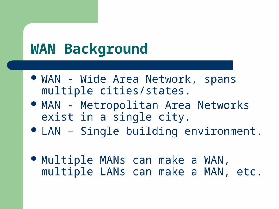
WAN Background

WAN - Wide Area Network, spans multiple cities/states.

MAN - Metropolitan Area Networks exist in a single city.

LAN – Single building environment.

Multiple MANs can make a WAN, multiple LANs can make a MAN, etc.

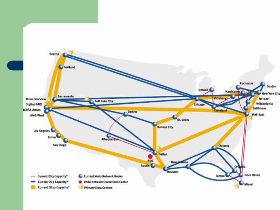
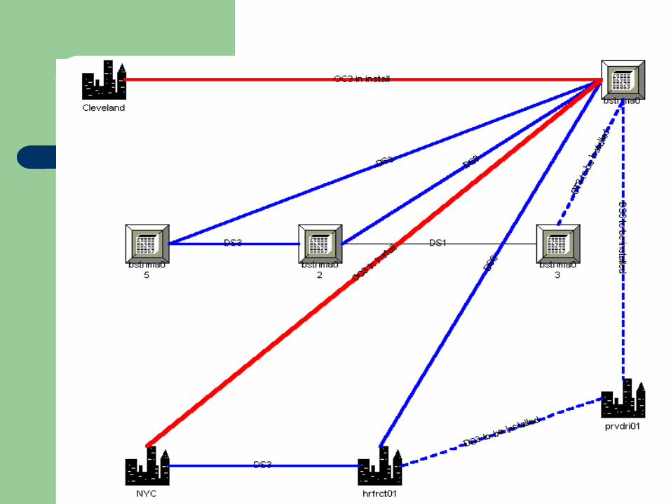
WAN Example

MAN As A Building Block

As I mentioned earlier, multiple MANs usually make up the WAN.

Each MAN has control of its own domain, but it’s uplink to the other MANs is considered the WAN (backbone).

Using Verio Boston’s example…

The Interconnects

MAN & WAN circuits must terminate in some form of a packet switch.

Using the UNet example from the other day, the packet switches were the Cisco Catalyst 6509 switches.

But keep in mind, the telephone company also has some switches in the field that handle even more traffic than what you’re getting!

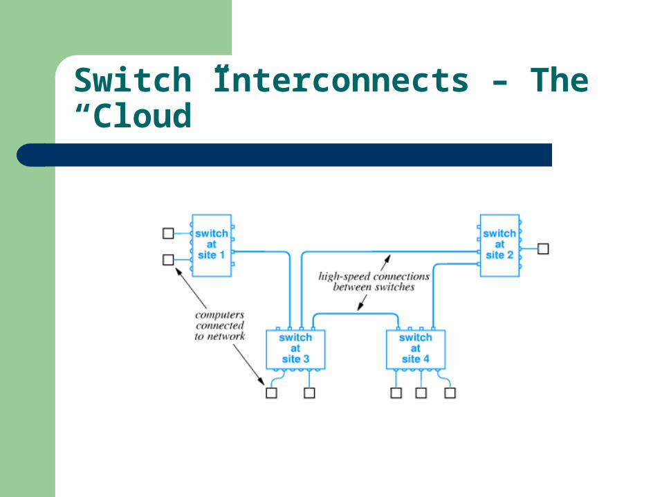
Switch Interconnects – The “Cloud”

WAN Switch Functionality

WAN switches use store and forward technology.

The store operation occurs when the packet arrives: the I/O hardware copies the packet, sticks it in memory, and signals the processor to forward the packet.

The forward operation is the act of removing the packet from memory, and sends it to the appropriate interface.

WAN Switch Functionality (cont.)

Storing the packets also leads to a form of queuing for each interface.

If the destination interface is busy, the packet is queued until the destination interface is idle, then the forward occurs.

The store and forward paradigm allows to handle the maximum bandwidth of the WAN connection, since all data is buffered!

Physical Addressing in the WAN Environment

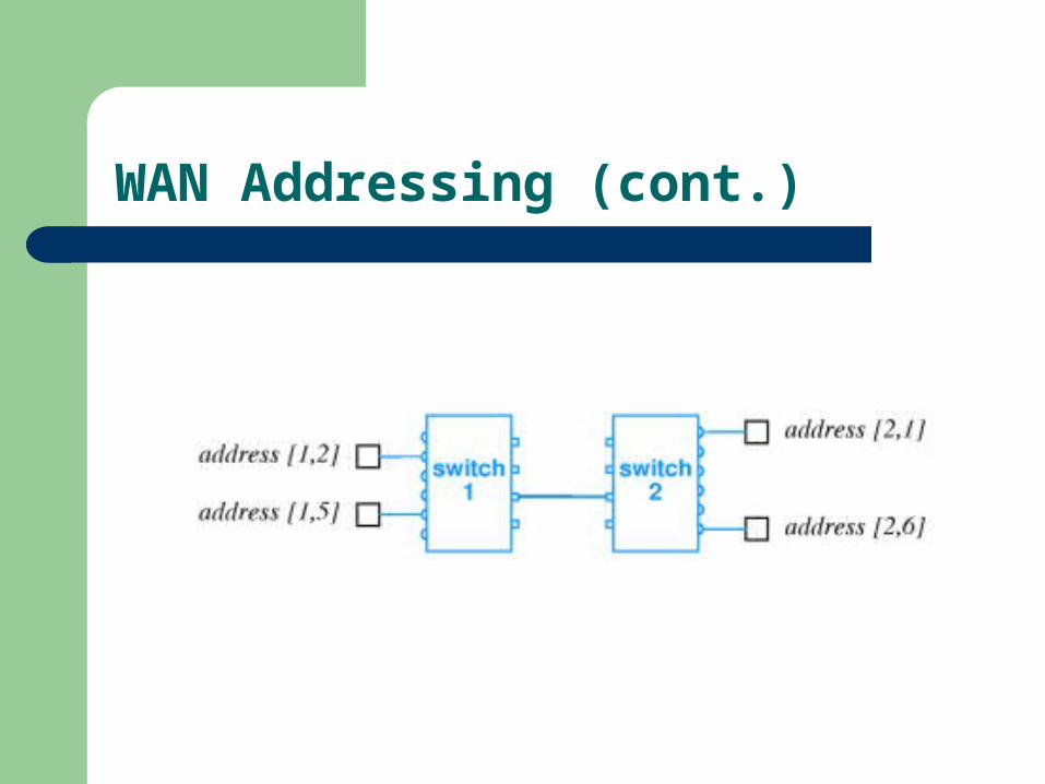
A hierarchical scheme is used with WAN addressing.

The simplest form of this scheme: The first part of the address holds the destination switch, the second part holds the specific machine that the packet is destined for on that switch.

This is scheme is used in many WAN environments.

WAN Addressing (cont.)

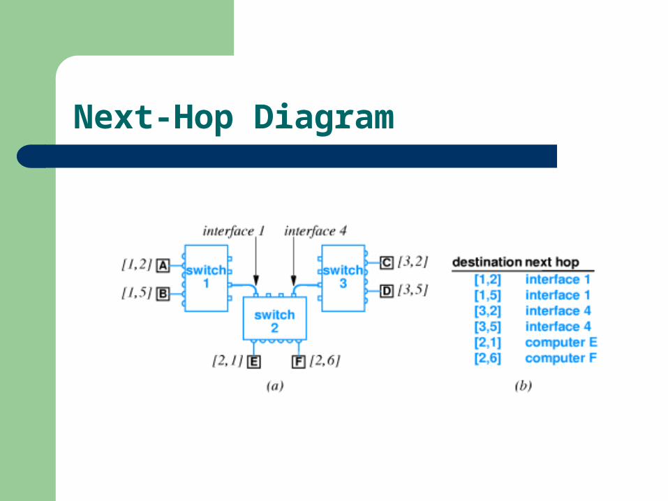
Next-Hop Forwarding

In order for networking to occur, each device must have some knowledge of the devices which it is connected to.

Next-hop forwarding is a scheme where devices know their neighbors, but don’t know the specifics of what is connected to each neighbor.

The Airline Example

– Suppose a passenger is traveling from San Francisco to Miami. Only one flight is listed, with three legs: Dallas, Atlanta, Miami.

– From San Francisco, his next destination is Dallas.– From Dallas, his next destination is Atlanta.– From Atlanta, his last destination is Miami.– But all along, the LAST destination was Miami, even

though the next hop was changing at each leg.

Next-Hop Diagram

Source Independence

The next hop does not depend on the direction that the packet came from.

This is referred to source independence. Source independence is a fundamental

concept in data networks. It allows for low-overhead, efficient networks.

Hierarchical Addressing & Routing

Heirarchical addressing is almost routing… The act of forwarding a packet to the next

address is dubbed routing. Routing uses a table format to determine the

next hop of the communication, and since it only needs to inspect the first part of the address, it is efficient!

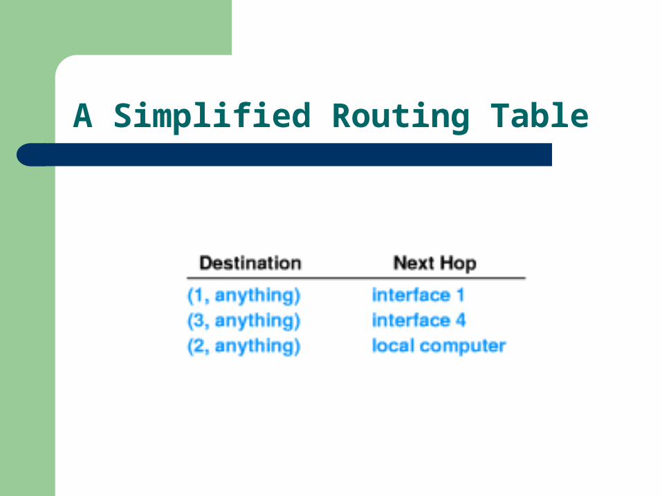
A Simplified Routing Table

Routing (cont.)

The two part addressing scheme provides us with the following:– Switches along the path of the transmission need to

inspect the first part of the hierarchical address.– The last switch in the transmission must inspect the

last part of the address.– Really efficient network transport! Not much

overhead.

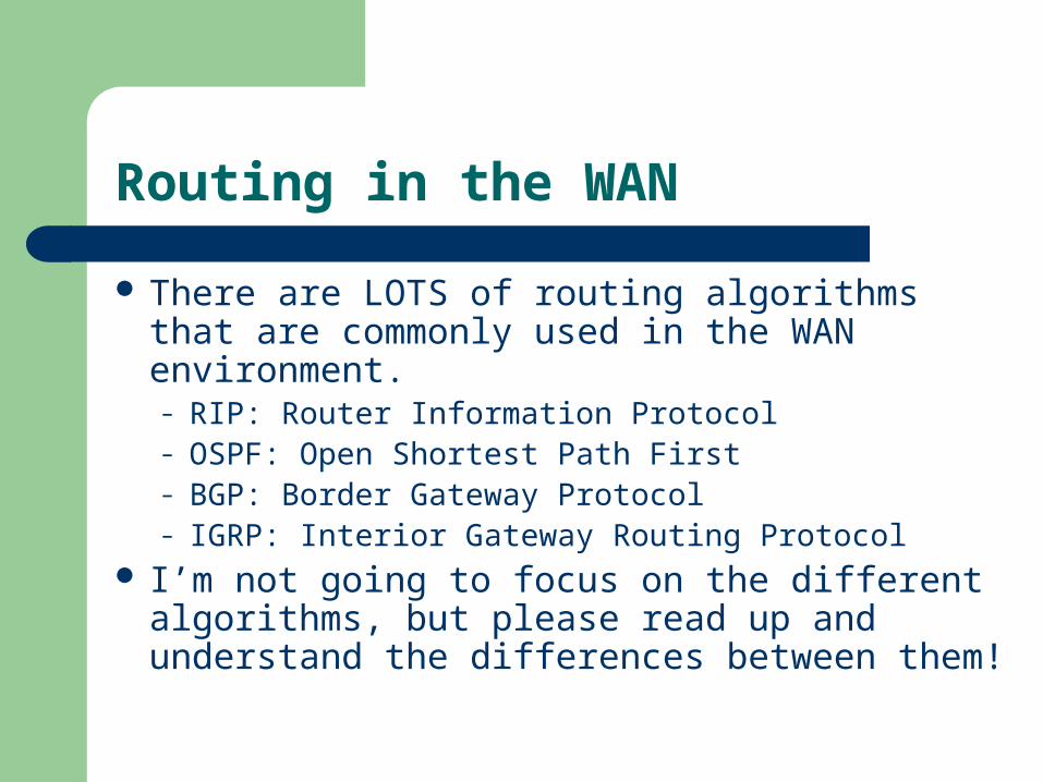
Routing in the WAN

There are LOTS of routing algorithms that are commonly used in the WAN environment.– RIP: Router Information Protocol– OSPF: Open Shortest Path First– BGP: Border Gateway Protocol– IGRP: Interior Gateway Routing Protocol

I’m not going to focus on the different algorithms, but please read up and understand the differences between them!

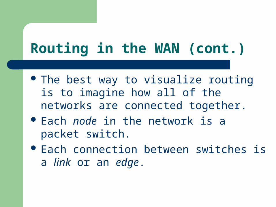
Routing in the WAN (cont.)

The best way to visualize routing is to imagine how all of the networks are connected together.

Each node in the network is a packet switch. Each connection between switches is a link or

an edge.

A Network Diagram

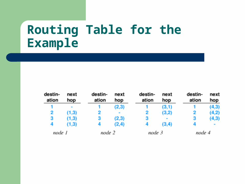
Routing Table for the Example

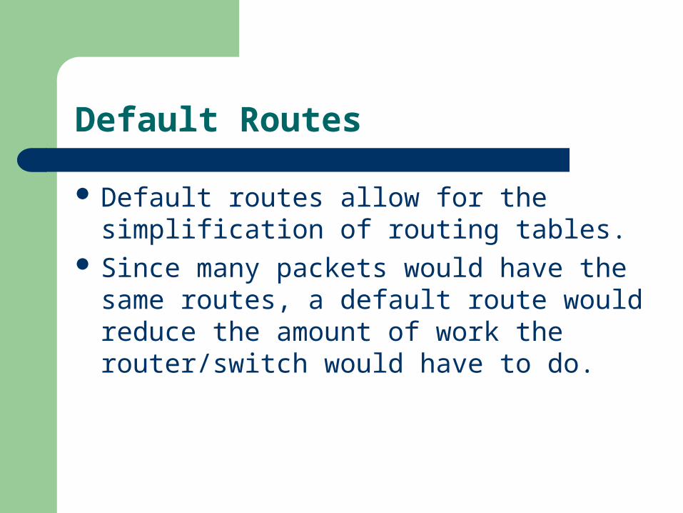
Default Routes

Default routes allow for the simplification of routing tables.

Since many packets would have the same routes, a default route would reduce the amount of work the router/switch would have to do.

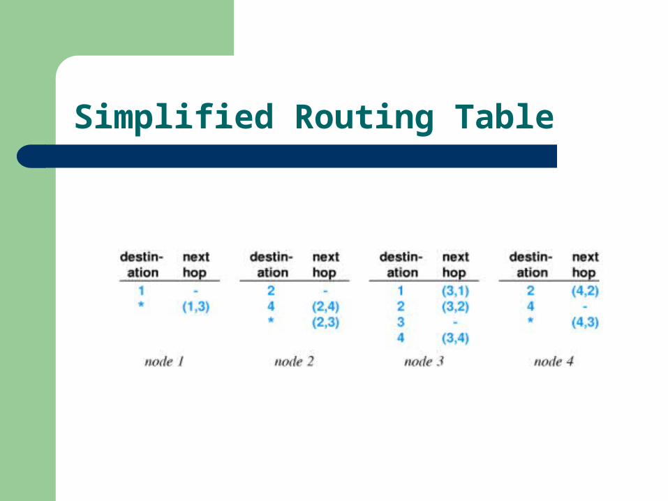
Simplified Routing Table

Default Routing (cont.)

Only one default route per device is allowed. The default route has lower priority to other

entered routes. If a transmission does not find a valid route, it

will send the packet down the default route.

Determination of the Routing Table

Two ways exist for route determination:– Static routing– Dynamic routing

Why have different options?

Static Routing

Static routing is the most straightforward of the two schemes.

Pros:– Simple to visualize– Low overhead on devices which perform routing

Cons:– Static, inflexible

Dynamic Routing

Dynamic routing can be very confusing. Multiple types of dynamic routing exist:

– OSPF– IGRP– BGP– RIP

Main disadvantage of dynamic routing: difficult to understand.

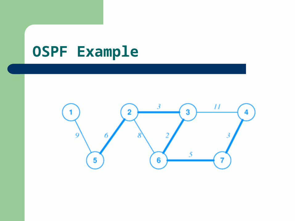
OSPF

OSPF – Open Shortest Path First Uses a system of metrics to determine route

preference. The entire route preference is the sum of the

individual metrics of the links between the computers.

The routers send their routing tables out periodically to their neighbors.

Common WAN Technologies

ATM- Asynchronous Transfer Mode Frame Relay SONET

ATM

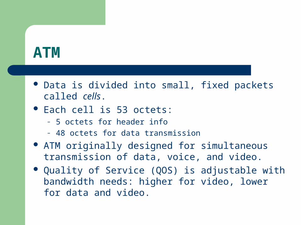
Data is divided into small, fixed packets called cells. Each cell is 53 octets:

– 5 octets for header info– 48 octets for data transmission

ATM originally designed for simultaneous transmission of data, voice, and video.

Quality of Service (QOS) is adjustable with bandwidth needs: higher for video, lower for data and video.

ATM (cont).

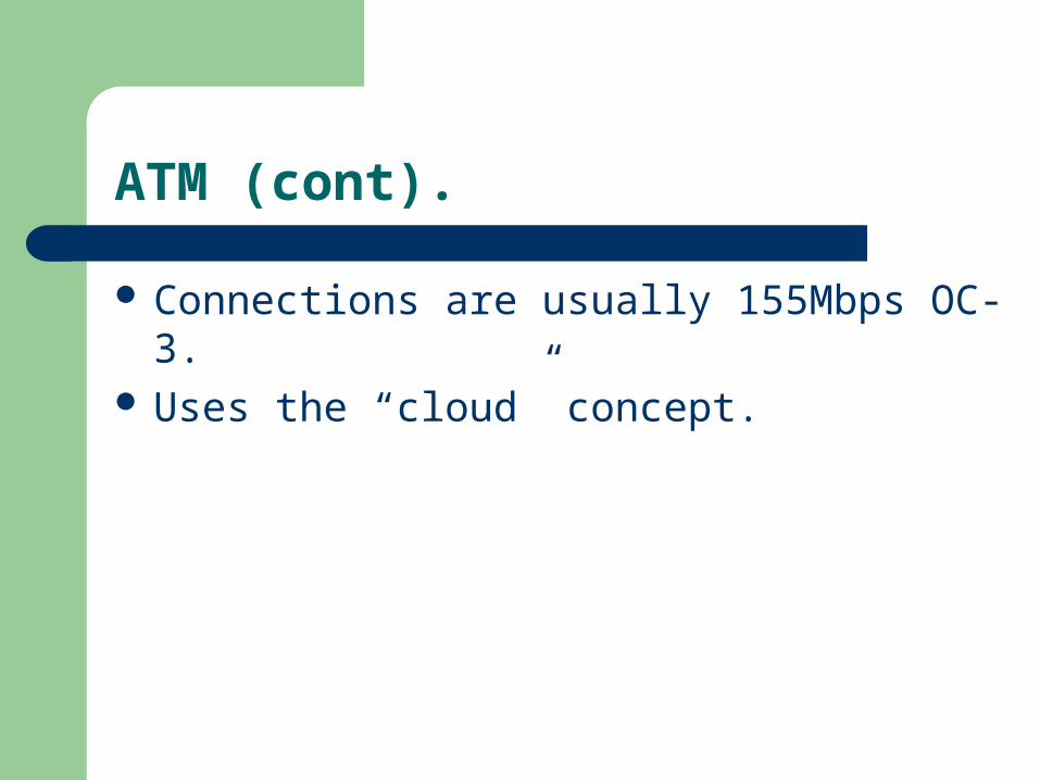
Connections are usually 155Mbps OC-3. Uses the “cloud” concept.

Frame Relay

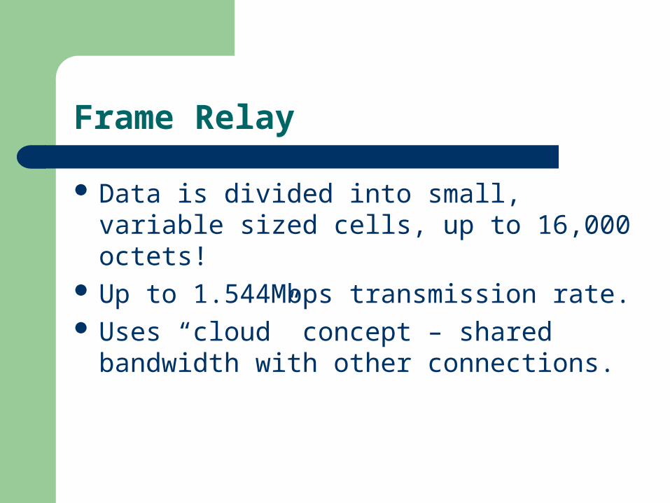
Data is divided into small, variable sized cells, up to 16,000 octets!

Up to 1.544Mbps transmission rate. Uses “cloud” concept – shared bandwidth with

other connections.

OSPF Example