Wall Crossing Invariants:from quantum mechanics to knots

D.Galakhova,b,∗, A. Mironovc,a,d,†and A. Morozova,d,‡

FIAN/TD-14/14ITEP/TH-28/14

a ITEP, Moscow 117218, Russiab NHETC and Department of Physics and Astronomy, Rutgers University, Piscataway, NJ 08855-0849, USA

c Lebedev Physics Institute, Moscow 119991, Russiad National Research Nuclear University MEPhI, Moscow 115409, Russia

Abstract

We offer a pedestrian level review of the wall-crossing invariants. The story begins from the scatteringtheory in quantum mechanics where the spectrum reshuffling can be related to permutations of S-matrices.In non-trivial situations, starting from spin chains and matrix models, the S-matrices are operator-valuedand their algebra is described in terms of R- and mixing (Racah) U-matrices. Then, the Kontsevich-Soibelman (KS) invariants are nothing but the standard knot invariants made out of these data within theReshetikhin-Turaev-Witten approach. The R and Racah matrices acquire a relatively universal form inthe quasiclassical limit, where the basic reshufflings with the change of moduli are those of the Stokes line.Natural from this point of view are matrices provided by the modular transformations of conformal blocks(with the usual identification R = T and U = S), and in the simplest case of the first degenerate field(2, 1), when the conformal blocks satisfy a second order Shrodinger-like equation, the invariants coincidewith the Jones (N = 2) invariants of the associated knots. Another possibility to construct knot invariantsis to realize the cluster coordinates associated with reshufflings of the Stokes lines immediately in terms ofcheck-operators acting on the solutions to the Knizhnik-Zamolodchikov equations. Then, the R-matricesare realized as products of successive mutations in the cluster algebra and are manifestly described in termsof quantum dilogarithms ultimately leading to the Hikami construction of knot invariants.

Contents1 Introduction 2

2 Wall crossing formulas as a piece of the WKB theory 42.1 Asymptotic behavior . . . . . . . . . . . . . . . . . . . . . . . . . . . . . . . . . . . . . . . . . . . 42.2 Jumps of WKB network topology on the curve . . . . . . . . . . . . . . . . . . . . . . . . . . . . 52.3 Non-trivial moduli space invariants: wall-crossing formulae in the moduli space . . . . . . . . . . 6

3 Classical problem of quantum mechanics: double well potential 7

4 Check- = “quantum, refined” 94.1 Intuitive remarks . . . . . . . . . . . . . . . . . . . . . . . . . . . . . . . . . . . . . . . . . . . . . 94.2 Beta-ensemble construction . . . . . . . . . . . . . . . . . . . . . . . . . . . . . . . . . . . . . . . 104.3 Determinant check-operator: quantizing the spectral curve . . . . . . . . . . . . . . . . . . . . . . 114.4 Higher weight operators and spectral covers . . . . . . . . . . . . . . . . . . . . . . . . . . . . . . 13∗galakhov@itep.ru; galakhov@physics.rutgers.edu†mironov@itep.ru; mironov@lpi.ru‡morozov@itep.ru

1

arX

iv:1

410.

8482

v1 [

hep-

th]

30

Oct

201

4

5 Knot invariants from WKB morphisms 155.1 Reidemeister invariants from quantum field theory . . . . . . . . . . . . . . . . . . . . . . . . . . 155.2 Knot invariants from RTW representation via duality kernels . . . . . . . . . . . . . . . . . . . . 17

5.2.1 The basic idea . . . . . . . . . . . . . . . . . . . . . . . . . . . . . . . . . . . . . . . . . . 175.2.2 S in (5.19) as the Racah matrix . . . . . . . . . . . . . . . . . . . . . . . . . . . . . . . . 185.2.3 S and T matrices from conformal theory . . . . . . . . . . . . . . . . . . . . . . . . . . . . 185.2.4 Plat representation of link diagrams (spherical conformal block) . . . . . . . . . . . . . . 20

5.3 Hikami knot invariants from check-operators . . . . . . . . . . . . . . . . . . . . . . . . . . . . . . 245.3.1 Quantum spectral curve in Chern-Simons theory . . . . . . . . . . . . . . . . . . . . . . . 245.3.2 Verlinde operators . . . . . . . . . . . . . . . . . . . . . . . . . . . . . . . . . . . . . . . . 255.3.3 Knots and flips . . . . . . . . . . . . . . . . . . . . . . . . . . . . . . . . . . . . . . . . . . 265.3.4 Hikami invariant as a KS invariant . . . . . . . . . . . . . . . . . . . . . . . . . . . . . . 27

5.4 Stokes phenomenon in conformal blocks . . . . . . . . . . . . . . . . . . . . . . . . . . . . . . . . 275.4.1 WKB approximation . . . . . . . . . . . . . . . . . . . . . . . . . . . . . . . . . . . . . . . 27

6 Conclusion and Discussion 30

1 IntroductionThe string theory approach to any problem is to consider it together with all possible deformations and as a

particular representation of some general structure appearing in many other, seemingly unrelated problems inother fields of science. One of the fresh application of this approach is the study of the wall-crossing phenomena(phase transitions) and associated invariants, which remain the same after the reshuffling. The outcome of thisstudy is that the Kontsevich-Soibelman (KS) invariants [1] found so far on this way, are probably not that new:they belong to an old class of invariants of the Reshetikhin-Turaev-Witten type, of which the most well-knownare knot invariants [2, 3]. At the same time, what naturally arises in wall-crossing problems, are quantumR-matrices in representations less trivial than the Verma modules of SUq(N), and this can further stimulatethe study of knot invariants in non-trivial representations.

An archetypical example of the wall-crossing is the spectrum dependence on the scattering potential inquantum mechanics. Consider a particle in the infinite well with some localized potential, for example:(

− ∂2x + uδ(x)− k2

)ψ(x) = 0, ψ(−L1) = ψ(L2) = 0 (1.1)

The spectrum k(u) is defined by the spectral equation

sin(kL1 + kL2

)− u

ksin(kL1) sin(kL2) = 0 (1.2)

and changes from the set

kn =πn

L1 + L2at u = 0 (1.3)

to a union of two sets1

kIn =πn

L1, kIIn =

πn

L2at u =∞ (1.4)

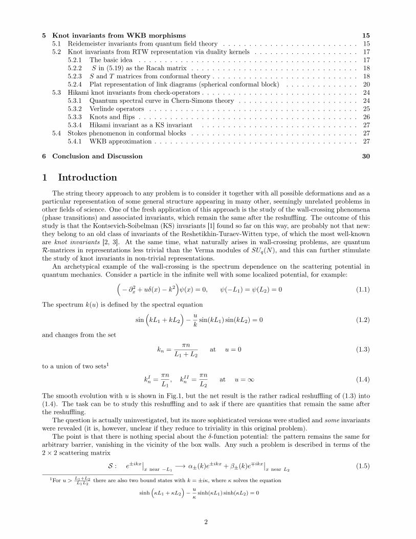
The smooth evolution with u is shown in Fig.1, but the net result is the rather radical reshuffling of (1.3) into(1.4). The task can be to study this reshuffling and to ask if there are quantities that remain the same afterthe reshuffling.

The question is actually uninvestigated, but its more sophisticated versions were studied and some invariantswere revealed (it is, however, unclear if they reduce to triviality in this original problem).

The point is that there is nothing special about the δ-function potential: the pattern remains the same forarbitrary barrier, vanishing in the vicinity of the box walls. Any such a problem is described in terms of the2× 2 scattering matrix

S : e±ikx∣∣x near −L1

−→ α±(k)e±ikx + β±(k)e∓ikx∣∣x near L2

(1.5)

1For u > L1+L2L1L2

there are also two bound states with k = ±iκ, where κ solves the equation

sinh(κL1 + κL2

)−u

κsinh(κL1) sinh(κL2) = 0

2

Figure 1: The picture of energy levels as function of u at L1 = 2L2 := 2L.

The spectral equation states that S converts sin(k(x+L1)

)∼ eik(x+L1)− e−ik(x+L1) into sin

(k(x−L2)

)∼

eik(x−L2) − e−ik(x−L2). For the δ-function potential, the scattering matrix is just

S =

1− u2ik − u

2ik

u2ik 1 + u

2ik

(1.6)

For the two isolated barriers, the scattering matrix is a product

S1 S2 = S1 ·(eikl12 0

0 e−ikl12

)· S2 (1.7)

where l12 is the distance between the two and so on: in general one has a product iSi.Changing the shape of the potential reduces to a composition of reshufflings, when constituents of the

product change order, i.e. to a composition of operations:

Kj : i<jSi Sj Sj+1 i>j+1 Si −→ i<jSi Sj+1 Sj i>j+1 Si (1.8)

This operation is of course very familiar: in the theory of quantum groups, if Si are the group elements [4, 5],this permutation is described by the quantum R-matrix, i.e. one can suspect that actually Kj = Rj and,further, Rj+1 = UjRjU†j , where U is the quantum mixing (Racah) matrix, see [6]. Then from this data it isstraightforward to build invariants: these are the ordinary knot invariants in the Reshetikhin-Turaev-Witten(RTW) formalism (graded traces and certain matrix elements of the ordered products of the R-matrices), whichin the context of wall-crossing theory are known as KS invariants.

To make this story really non-trivial, one needs to promote scattering matrices S to operator-valued quan-tities S. In quantum group theory this is achieved by making the elements of the algebra of functions non-commutative, in quantum mechanics it is enough to introduce internal degrees of freedom like spins or, moregenerally, to consider matrix models (e.g. matrix quantum mechanics). This makes R- and U-matrices differentfrom just ordinary permutation matrices: they start to realize the far less simple braid group structures.

Emergence of braids is, of course, not universal for quantum mechanical problems, they arise only when thespace is 2-dimensional and there are topologically different ways to adiabatically carry one point around another,producing a Berry phase. This is, however, a generic situation for algebraically integrable dynamics, where theseparation of variables reduces the study to a complex curve (sometime called spectral or Seiberg-Witten curve,the Liouville torus being its Jacobian). Though formally integrable systems are pretty rare, there is a growingevidence that typical effective field theory obtained after integration over fast variables is integrable [5, 7], andthis explains the growing interest to this type of theories.

Even in this integrability context, naturally appearing representations of the braid group can be quitesophisticated and difficult to study. Still there are two immediate classes of examples (in addition to theordinary Verma modules of ordinary quantum groups like SUq(N) widely used in conventional knot theory).One of them is provided by the WKB limit of quantum mechanics, where the R-matrices actually describereshufflings of the Stokes lines. Another one is provided by the modular transformations of conformal blocks:the modular kernels Ti and Si provide an interesting set of Ri and Ui matrices, which can be used to constructa priori new families of knot invariants. In the simplest case, however, the family is not new: one gets just the

3

ordinary Jones polynomials (and probably HOMFLY at the next step), but more sophisticated examples seemcapable to provide a long awaited group theory (RTW) interpretation of the Hikami invariants.

The plan of the paper is as follows.We begin in sec.2 from the general review of the WKB approach involving the theory of Stokes lines, their

reshufflings and KS invariants.Then, in sec.3 we consider from this perspective the standard example of the double-well potential.After that, in sec.4 we switch to matrix models and reformulate the problem in terms of the operator-valued

(check) resolvents.In sec.5 we consider KS/RTW invariants, associated with the simplest knots and links and show that the

R-matrices, provided by the modular transformations of conformal blocks, give rise to various types of knotinvariants: the Jones polynomials and the Hikami integrals.

A natural part of this presentation are the distinguished (Fock-Goncharov [8]) coordinates on the modulispace provided by the WKB theory, where the R-matrices act via peculiar rational transformations (known alsoas mutations in cluster algebra [9] and related to discrete change of coordinates in the algebra of functions [10]).

Conclusion in sec.6 describes (incomplete) list of relations between different subjects in theoretical physics,which are brought together by consideration of the wall-crossing phenomena.

2 Wall crossing formulas as a piece of the WKB theory

2.1 Asymptotic behaviorIn Seiberg-Witten (SW) theory describing the low-energy limit of N = 2 supersymmetric gauge theory [11],

the central charge and the mass of an excitation are given by the contour integrals of the SW differential λ:

Zγ =

∮γ

λ, Mγ =

∮γ

|λ| (2.1)

BPS states have M = |Z|, therefore they are associated with the Stokes contours σ(x) ∈ Σ on the spectralsurface Σ, such that the Seiberg-Witten differential λ (which is a meromorphic differential on Σ whose variationswith respect to moduli are holomorphic) along these contours has a definite phase φσ:

Arg(e−iφσλ

[σ(x)

])= 0 (2.2)

so that

Arg

(e−iφσ

∫σ(x)

λ

)= 0 (2.3)

If the gauge theory is described via M-theory [12], then these σ are interpreted as intersections of the main M5-brane with the M2-branes, see [13]. The spectral surface Σ is a ramified covering of the original bare curve Σ0,and λ is the eigenvalue of the Lax 1-form [14]. The mass of the BPS state is given by the absolute value of thesame integral, and the mass is finite when the contour is closed. To make the Stokes contour closed, one shouldadjust the phase φσ, this possibility to adjust the phase of the Planck constant is the main new peculiarityof the BPS state counting as compared to the usual WKB theory. When the moduli of the spectral surfacechange, so do the phase and the shape of the contour, and at some values of moduli the change can be abrupt:discontinuous. Such a jump in the multiplicities of the BPS states takes place along the real-codimension-onesurfaces in the moduli space and is called the wall-crossing phenomenon. What remains invariant are peculiarcombinations of multiplicities, encoded in the form of Kontsevich-Soibelman formula.

Our purpose in this paper is to discuss a pedestrian approach to this kind of problems, relating them to theelementary textbook consideration of Stokes phenomena for the WKB approximation.

For this purpose we consider the Wilson line

WΓ(φ) = P exp

(ieiφ

~

∫Γ

L)

(2.4)

of the N × N -matrix valued Lax form along an open contour Γ ∈ Σ0 on the bare Riemann surface Σ0. TheN eigenvalues of L define the Seiberg-Witten differential λi on the N sheets of the spectral surface Σ which Ntimes covers Σ0, so that one can roughly write WΓ(φ) as

wΓ(φ) = diag

exp

(ieiφ

~

∫γi

λi

)(2.5)

4

where γi are pre-images of Γ on Σ. However, if one wishes to treat wΓ as a quasiclassical approximation to anevolution operator for some quantum-mechanical system, then one should switch between different branches iwhen Γ crosses the Stokes lines. For example, if one has a two-sheet covering with λ± = ±λ, and one considers

Figure 2: Intersecting one Stokes line.

the evolution along the contour, which goes from the point A to B and crosses a Stokes line, originating atramification point P (see Fig.2), then

Ψ(B) =

(ψ(B+)ψ(B−)

)=

exp

(ieiφ

~∫ B+

A+λ)

exp(ieiφ

~

(∫ B+

Pλ−

∫ PA−

λ))

0 exp(− ie

iφ

~∫ B−A−

λ)

( ψ(A+)ψ(A−)

)(2.6)

while for the inverse path from B to A one would rather encounter a low-triangular matrix. Thus, instead of thenaive wΓ one gets for the quasiclassical Abelization of the Wilson operator WAB(φ) a sum of three elementarymatrices

Ψ(B) =(wB+A+

(φ) + wB+PA−(φ) + wB−A−(φ))

Ψ(A) (2.7)

Figure 3: Intersecting two Stokes lines.

2.2 Jumps of WKB network topology on the curveLet us call the set of WKB lines (WKB network) Γ ∈ Σ0 such that its preimages compose the contour σ

satisfying (2.2). The WKB network gives a triangulation of the spectral surface Σ0. This triangulation dependson the phase φ and it can jump at some specific critical values φc making a kind of flips of the triangulation.

When a flip occurs, two different Stokes lines merge into a single line of finite length (we denote its pre-image on Σ as γc) so that the integral (2.1) giving the central charge Zγc =

∮γc

λ becomes convergent. We can

immediately define the value of the critical phase as

φc = ArgZγc (2.8)

Now we observe how the value of the asymptotic expansion of a Wilson operator changes. If two Stokeslines which originate at the ramification points P1 and P2 were crossed on the way from A to B (see Fig.3), wewould obtain a Wilson operator

WAB(φ−) = wB+A+(φ−) + wB−A−(φ−) + wB+P1A−(φ−) + wB−P2A+(φ−) + wB−P2P1A−(φ−) =

= wB+A+(φc) + (1 + wσ)wB−A−(φc) + wB+P1A−(φc) + wB+P2A−(φc)

(2.9)

5

where φ− = φc − 0. For the other value of phase φ+ = φc + 0 configuration of the Stokes lines can be different,and one obtains another decomposition

WAB(φ+) = wB+A+(φ+) + wB+P1A−(φ+) + wB−P2A+(φ+) + wB−P1P2A−(φ+) =

= (1 + wσ)wB+A+(φc) + wB−A−(φc) + wB+P1A−(φc) + wB+P2A−(φc)(2.10)

differing not only by the value of φ but also by reordering of the points P1 and P2. At the critical value φc ofphase, where reshuffling of the Stokes lines occurs and a closed Stokes line σ appears, the two expressions differexactly by wσ, i.e. an abrupt reshuffling takes place

WAB −→ KσWAB (2.11)

where a morphism K acts as

Kσ : wα = (1 + wσ)<σ,α>wα (2.12)

Note that this is not an ordinary operator. This morphism acts as a change of coordinates on the modulispace of flat connections. So we apply it to every term in the sum independently, in detail:

Kσ(WAB(φ−)) = Kσ(wB+A+(φc)) + (1 + Kσ(wσ))Kσ(wB−A−(φc)) + Kσ(wB+P1A−(φc)) + Kσ(wB+P2A−(φc)) =

= (1 + wσ)

〈σ,B+A+〉︸ ︷︷ ︸1 wB+A+(φc) +

1 + (1 + wσ)

〈σ, σ〉︸ ︷︷ ︸0 wσ

(1 + wσ)

〈σ,B−A−〉︸ ︷︷ ︸−1 wB−A−(φc)+

+(1 + wσ)

〈σ,B+P1A−〉︸ ︷︷ ︸0 wB+P1A−(φc) + (1 + wσ)

〈σ,B+P2A−〉︸ ︷︷ ︸0 wB+P2A−(φc) = WAB(φ+)

(2.13)

2.3 Non-trivial moduli space invariants: wall-crossing formulae in the modulispace

As we have seen the asymptotics of Wilson lines is not smooth. The discontinuity is of order wσ(φc), whichis asymptotically small.

Nevertheless, the very value of the observable is expected to be smooth. This fact allows one to constructnon-trivial invariants of the morphisms K on the Coulomb branch, called spectrum generators [53] tightlyrelated to the spectra of BPS states arising in the effective theory.

In general, when one starts increasing the phase φ from 0 to π, a number of reshufflings take place, whenparticular closed Stokes lines σa appear at critical values φa, and disappear with the further increase of φ. Thisprovides a sequence of actions

←−∏a

Kσa (2.14)

The number of factors here is actually the number of BPS states on the given spectral curve, i.e. at the givenpoint of the moduli space. If one now starts changing moduli of the spectral curve this very product can change,reflecting the change of the ordered set A of the BPS states, including their number (the number of factors inthe product), and the order in which they occur with increase of the phase φ. However, at the domain wallin moduli space (at the hypersurface of marginal stability) given by the condition φ = φc the two differentproducts should coincide:

←−−∏a∈A

Kσa =←−∏b∈B

Kσb (2.15)

thus we obtain the Kontsevich-Soibelman (KS) invariant, taking values in functors, acting on the space ofw-variables often called the Fock-Goncharov coordinates of the flat connection moduli space.

Basic example: For two conjugated A and B cycles on a torus with < A,B >= 1 the KS relation states:

KAKB = KBKA+BKA (2.16)

6

where the operator action is defined as

KmA+nBwγ = (1 + wmAwnB)m<A,γ>+n<B,γ>wγ (2.17)

Note that the coordinates wAwB = wBwA commute, and also wA+B = wAwB , while neither of these is true forthe operators K. With these definitions eq.(2.16) is just an identity, indeed, applying both sides to, say wA,one gets

KAKBwA = KA1

1 + wBwA =

1

1 + (1 + wA)wBwA =

wA1 + wB + wAwB

, (2.18)

and

KBKA+BKAwA = KBKA+BwA = KB1

1 + wAwBwA =

1

1 + 11+wB

wAwB· 1

1 + wBwA =

wA1 + wB + wAwB

(2.19)

Similarly, in application to wB :

KAKBwB = (1 + wA)wB , (2.20)

and

KBKA+BKAwB = KBKA+B(1 + wA)wB = KB

(1 +

1

1 + wAwBwA

)(1 + wAwB)wB =

=

(1 +

1

1 + 11+wB

wAwB

1

1 + wBwA

)(1 +

1

1 + wBwAwB

)wB =

1 + wA + wB + wAwB1 + wB

wB = (1 + wA)wB

3 Classical problem of quantum mechanics: double well potentialConsider the Schrodinger equation with the quartic potential[

~2∂2z − (z − x1)(z − x2)(z − x3)(z − x4)

]Ψ(z) = 0 (3.1)

Depending on the choice of zeroes xk, the structure of levels is rather different.At the first glance, this may seem a little bit controversial. According to the well-known theorem in ODE

theory, solutions to the Cauchy problem are continuous functions of parameters if the coefficients of equation arecontinuous. Nevertheless, the problem of finding eigenvalues of self-adjoint operators (Sturm-Liouville problem)is quite different. Once found integrable in the usual Hilbert norm, the eigenfunctions at some chosen values ofparameters are not expected to keep integrability at another choice of the parameters.

The integrability of function depends on its asymptotic behavior. In this particular case there are twoasymptotics e±

z3

~ . Choose two linearly independent solutions Ψ1,2 with the asymptotics behaviour being

Ψ1(z) ∼z→±∞

c1+(±∞)ez3

~ + c1−(±∞)e−z3

~ (3.2)

Ψ2(z) ∼z→±∞

c2+(±∞)ez3

~ + c2−(±∞)e−z3

~ (3.3)

We define an “S-matrix” as

S =

(σ++ σ−+

σ+− σ−−

)=

(c1+(+∞) c1−(+∞)c2+(+∞) c2−(+∞)

)−1(c1+(−∞) c1−(−∞)c2+(−∞) c2−(−∞)

)(3.4)

Note that this matrix is independent of the choice of the basis in solutions. For a generic choice of parametersthis S-matrix is unphysical.

To define an eigenfunction we require it to be integrable for real ~, i.e. to behave as

Ψ(z) ∼z→±∞

e∓z3

~ (3.5)

This imposes a condition on the S-matrix entries

σ−−(x1, x2, x3, x4) = σ++(x1, x2, x3, x4) = 0 (3.6)

The crucial point is that the S-matrix is discontinuous on the moduli space (xk, ~) (see also [15]).To observe this, we consider two well-known physical situations:

7

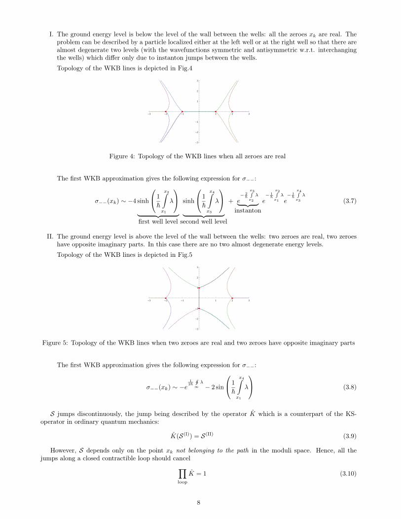
I. The ground energy level is below the level of the wall between the wells: all the zeroes xk are real. Theproblem can be described by a particle localized either at the left well or at the right well so that there arealmost degenerate two levels (with the wavefunctions symmetric and antisymmetric w.r.t. interchangingthe wells) which differ only due to instanton jumps between the wells.

Topology of the WKB lines is depicted in Fig.4

-3 -2 -1 1 2 3

-3

-2

-1

1

2

3

Figure 4: Topology of the WKB lines when all zeroes are real

The first WKB approximation gives the following expression for σ−−:

σ−−(xk) ∼ −4 sinh

1

~

x2∫x1

λ

︸ ︷︷ ︸first well level

sinh

1

~

x4∫x3

λ

︸ ︷︷ ︸second well level

+ e− 2

~

x3∫x2

λ︸ ︷︷ ︸instanton

e− 1

~

x2∫x1

λ

e− 1

~

x4∫x3

λ

(3.7)

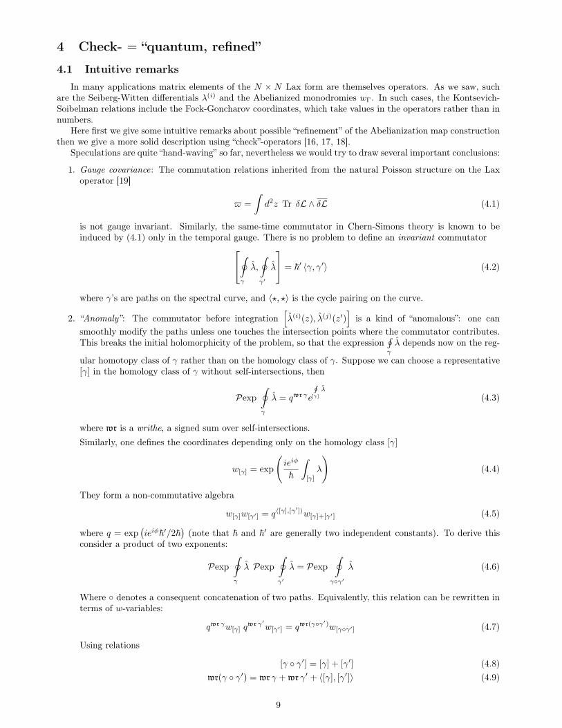
II. The ground energy level is above the level of the wall between the wells: two zeroes are real, two zeroeshave opposite imaginary parts. In this case there are no two almost degenerate energy levels.

Topology of the WKB lines is depicted in Fig.5

-3 -2 -1 1 2 3

-3

-2

-1

1

2

3

Figure 5: Topology of the WKB lines when two zeroes are real and two zeroes have opposite imaginary parts

The first WKB approximation gives the following expression for σ−−:

σ−−(xk) ∼ −e12~∮∞λ− 2 sin

1

~

x4∫x1

λ

(3.8)

S jumps discontinuously, the jump being described by the operator K which is a counterpart of the KS-operator in ordinary quantum mechanics:

K(S(I)) = S(II) (3.9)

However, S depends only on the point xk not belonging to the path in the moduli space. Hence, all thejumps along a closed contractible loop should cancel∏

loop

K = 1 (3.10)

8

4 Check- = “quantum, refined”

4.1 Intuitive remarksIn many applications matrix elements of the N × N Lax form are themselves operators. As we saw, such

are the Seiberg-Witten differentials λ(i) and the Abelianized monodromies wΓ. In such cases, the Kontsevich-Soibelman relations include the Fock-Goncharov coordinates, which take values in the operators rather than innumbers.

Here first we give some intuitive remarks about possible “refinement” of the Abelianization map constructionthen we give a more solid description using “check”-operators [16, 17, 18].

Speculations are quite “hand-waving” so far, nevertheless we would try to draw several important conclusions:

1. Gauge covariance: The commutation relations inherited from the natural Poisson structure on the Laxoperator [19]

$ =

∫d2z Tr δL ∧ δL (4.1)

is not gauge invariant. Similarly, the same-time commutator in Chern-Simons theory is known to beinduced by (4.1) only in the temporal gauge. There is no problem to define an invariant commutator∮

γ

λ,

∮γ′

λ

= ~′ 〈γ, γ′〉 (4.2)

where γ’s are paths on the spectral curve, and 〈?, ?〉 is the cycle pairing on the curve.

2. “Anomaly”: The commutator before integration[λ(i)(z), λ(j)(z′)

]is a kind of “anomalous”: one can

smoothly modify the paths unless one touches the intersection points where the commutator contributes.This breaks the initial holomorphicity of the problem, so that the expression

∮γ

λ depends now on the reg-

ular homotopy class of γ rather than on the homology class of γ. Suppose we can choose a representative[γ] in the homology class of γ without self-intersections, then

Pexp

∮γ

λ = qwr γe

∮[γ]

λ

(4.3)

where wr is a writhe, a signed sum over self-intersections.Similarly, one defines the coordinates depending only on the homology class [γ]

w[γ] = exp

(ieiφ

~

∫[γ]

λ

)(4.4)

They form a non-commutative algebra

w[γ]w[γ′] = q〈[γ],[γ′]〉w[γ]+[γ′] (4.5)

where q = exp(ieiφ~′/2~

)(note that ~ and ~′ are generally two independent constants). To derive this

consider a product of two exponents:

Pexp

∮γ

λ Pexp

∮γ′

λ = Pexp

∮γγ′

λ (4.6)

Where denotes a consequent concatenation of two paths. Equivalently, this relation can be rewritten interms of w-variables:

qwr γw[γ] qwr γ′w[γ′] = qwr(γγ′)w[γγ′] (4.7)

Using relations

[γ γ′] = [γ] + [γ′] (4.8)wr(γ γ′) = wr γ + wr γ′ + 〈[γ], [γ′]〉 (4.9)

9

one reproduces algebraic relation (4.5). The second relation says that the writhe function is a quadraticrefinement of the intersection form, for details see [20, Appendix C].As in the previous section, the Wilson lines are polynomials in w-variables, though now over Z[q, q−1]

Tr Pexp

∮L ∼

∑γ

qwr γw[γ] (4.10)

To conclude this section we mention that this quite heuristic consideration can be applied to physicalproblems [20]. K-jumps of expansion (4.10) similarly to the jumps discussed in the previous section allow oneto calculate characteristics of the BPS spectra in N = 2 SYM theories. These invariants are refined now witha deformation parameter q and take into account the spin of BPS multiplets.

4.2 Beta-ensemble constructionBeta-ensembles naturally extend matrix models and inherit their basic properties. The model is given by

the partition function of 2d Coulomb gas (here we consider an example when the gas is placed on the sphere)

Z =∏i

∮γi

dzi∏i<j

(zi − zj)2βe− 1g

∑iV (T |zi)

(4.11)

where g, β are two parameters similar to ~ and ~′, and the potential V (T |z) determines the moduli space of thepartition function: it is parameterized by the parameters Tk of the potential and by the choice of the integrationcontours. For the sake of definiteness, we choose the potential to be a polynomial and Tk to be coefficients ofthis polynomial:

V (z) =

n∑k=0

Tkzk (4.12)

We consider only closed contours so that changing the variables

zi → zi +ε

ζ − zi(4.13)

does not change the integral, which leads to the following Ward identity in the first order of ε⟨∑i

1

(ζ − zi)2+ β

∑i 6=j

1

(ζ − zi)(ζ − zj)− 1

g

∑i

V ′(zi)

⟩= 0 (4.14)

After some algebra this equation can be represented in the following form

(β − 1)∂ζ

⟨∑i

1

ζ − zi

⟩+ β

⟨(∑i

1

ζ − zi

)2⟩− V ′(ζ)

g

⟨∑i

1

ζ − zi

⟩+

1

g

⟨∑i

V ′(ζ)− V ′(zi)ζ − zi

⟩= 0 (4.15)

Let us define the resolvent as

ρ(ζ) :=1

Z∇(ζ)Z := g

√β

⟨∑i

1

ζ − zi

⟩(4.16)

where the operator ∇(ζ) can be described by the action of g√β∑

1zk+1

∂∂tk

on the partition function with themodified potential V (z)→ V (z)− g

∑k tkz

k, treated as a formal (perturbative) series in the variables tk:

Z =∏i

∮γi

dzi∏i<j

(zi − zj)2βe− 1g

∑iV (T |zi)+

∑i,k tkz

ki

(4.17)

We use Z for the partition function Z restricted to all tk = 0.The last term in (4.15) can be reproduced by the action of the differential operator in Tk’s:

P (ζ) = −g2n∑k=2

kTk

k−2∑n=0

ζn∂Tk−2−n (4.18)

10

We call such operators check-operators since they act on moduli Tk’s (in variance with ∇(ζ)). Note that theMiwa transform of Tk-moduli

Tk =∑j

αjλkj

k(4.19)

transforms the check-operator P (ζ) into

P (ζ) ∼∑j

∂λjζ − λj

(4.20)

One also can introduce the check-operator that generates the resolvents:

∇Z = ∇Z (4.21)

This operator can be constructed recursively from y :=√V ′(T |z)2 − 4βP , its derivatives and V ′(T |z) [17]. The

recursion is provided by the g2-expansion, and, in the leading order, ∇(0) = g√βy.

Then the Ward identity can be rewritten in the form[gQ∂ζ∇(ζ) + :∇(ζ)2:− V ′(ζ)√

β∇(ζ) + P (ζ)

]Z = 0 (4.22)

where Q :=√β − 1√

βand the normal ordering means that the operator ∇(ζ) acts only on Z, but not on itself.

4.3 Determinant check-operator: quantizing the spectral curveIn the leading order of the WKB approximation (i.e. g2 → 0), the Ward identity (4.22) becomes the algebraic

equation for the resolvent (4.16):

ρ(0)(ζ)2 − V ′(ζ)√βρ(0)(ζ) + f(ζ) = 0 (4.23)

where the polynomial f(ζ) := P logZ. This algebraic equation is nothing but the spectral curve. Note thatthe monodromies of these check-operators along A- and B-periods of these spectral curve form the Heisenbergalgebra [17]: [∮

Ai

∇(ζ)dζ,

∮Bj

∇(ζ)dζ

]= δij (4.24)

One may ask what are the ways of quantizing the spectral curve (4.23) (which has to become the Baxterequation after quantization). There are two possibilities. One of the possibilities is to consider the limit of(4.11) when g2/β = ~′2 → 0 with g2β = ~2 kept fixed. In this limit (called Nekrasov-Shatashvili limit [21])the Ward identity (4.22) gets the Ricatti (or Schrodinger) equation equivalent to the Baxter equation [22] andcorresponding to a quantum integrable system [21, 23, 24, 25, 26].

However, this system depends only on one parameter g√β = ~. However, there is a possibility of quantizing

the spectral curve which still preserves the β-ensemble representation for the wavefunction and depends on twoparameters β, g. To this end, in [24] it was suggested to consider the equation for the β-ensemble average ofthe would-be determinant in matrix model: the average Ψ(ζ) = 〈

∏i(ζ − zi)〉. To dealing with this average, one

introduces another check-operator:

1

ZD[1](ζ)Z :=

⟨∏i

(ζ − zi)

⟩(4.25)

In order to understand the meaning of Ψ(ζ) let us rewrite it as (the number of integrations in the β-ensemblepartition function is denoted through N)

Ψ(ζ) = ζN

⟨∏i

(1− zi

ζ

)⟩= ζN

⟨exp

∑i

(1− zi

ζ

)⟩= ζN

⟨exp

(−∑k

∑i zki

kζk

)⟩(4.26)

11

This expression is equal both to

Ψ(ζ) = ζN1

Zexp

(∫ ζ

dz∑k

1

zk+1

∂

∂tk

)Z =

exp(

1~∫ ζdz∇(z)

)Z

Z(4.27)

where N is treated as zero time t0, and to

Ψ(ζ) =Z(tk − 1

kζk

)Z(tk)

(4.28)

Let us consider the case of β = 1 when the β-ensemble reduces to the Hermitean matrix model. Within theAGT, this case corresponds to the conformal field theory with central charge 1 [27, 28]. In this case, Z is aτ -function of the Toda-chain hierarchy [29] in time variables tk, and Ψ(ζ) given by formula (4.28) is the Baker-Akhiezer function. It corresponds to insertion of the fermion ψ(ζ) at the point ζ (and a fermion ψ at infinity).This can be easily understood, since in c = 1 theory (free fields) the fermion is described in terms of the freefield φ(ζ) by the exponential : exp(iφ(ζ)) : which being inserted into the conformal correlator representationof the matrix model [30] gives exactly the determinant [24]. This fermion describes the simplest fundamentalrepresentation of the SL(N) group which can be understood from the realization of its N -plet as [31]

ψi|0 >= T i−1− |0 > (4.29)

where the fermion modes are defined by ψ(ζ) =∑Ni ψiζ

i and T− =∑N−1i T−αi is the sum of all raising

operators associated with the negative simple roots of SL(N). Then all other fundamental representationsare defined as products of fermions. This connection with the fundamental representations can be also mademanifest via the expansion of the determinant into the fundamental representations:∏

i

(1− zi

ζ

)=∑k

χ[1k](zi)

(−1

ζ

)k(4.30)

where χ[1k](zi) is the Schur function, i.e. the characters of group SL(N) associated with the fundamentalrepresentations.

One now can convert the Ward identity (4.22) into the equation for Ψ(ζ). To this end, one needs to rewritethe Ward identity in terms of shifted time-variables and of operators acting on Z:[

gQ∂ζ∇(ζ) + ∇(ζ)2 − 1√β

(V ′(tk −

1

kζk

∣∣∣ζ)∇(ζ)

)−

]Z(tk −

1

kζk

)= 0 (4.31)

where the subscript "-" refers to negative powers of ζ and ∇(ζ) does not need to be normal ordered, since itdoes not act on itself. We will use further(

V ′(tk −

1

kζk

∣∣∣ζ)∇(ζ)

)−

= g√β∑n≥−1

1

ζn+2

∑k≥1

k

(tk −

1

kζk

)∂

∂tk+n=

=(V ′(t|ζ)∇(ζ)

)−− g√β∑k,n

1

ζk+n+2

∂

∂tk+n=(V ′(t|ζ)∇(ζ)

)−− ∂ζ∇(ζ) (4.32)

where at the last step we compared the coefficient k+1 in ∂ζ∇(ζ) = g√β∑m≥0

m+1zm+2

∂∂tm

with∑

k≥1

n≥−1δk+n,m =

m+ 1.Since, for the “non-normalized” Ψ(ζ) := Z

(tk − 1

kζk

), one directly checks that g

√β∂ζΨ(ζ) = ∇(ζ)Ψ(ζ) and

g2β∂2ζ Ψ =

(∇2(ζ) + g

√β∂ζ∇(ζ)

)Ψ(ζ), one finally obtains a differential equation

[g2β∂2

ζ − V ′(ζ)∂ζ + P (ζ, Tk)]

Ψ(ζ) = 0 (4.33)

which is a quantization of the algebraic spectral curve which depends on the both parameters of deformationg and β. With rescaling the wave function Ψ(ζ) = exp

(V (ζ)/(g2β)

)Ψ(ζ), one can recast this equation to the

form [g2β∂2

ζ +1

2

(V ′′(ζ)− V ′2(ζ)

2g2β+

1

g2β

[P (ζ, Tk)V (ζ)

])+ P (ζ, Tk)

]Ψ(ζ) = 0 (4.34)

12

Now one can easily construct action of the determinant check operator on the partition function using (4.27):⟨∏i

(ζ − zi)

⟩Z = e

1~

ζ∫dz∇(z)Z = :e

1~

ζ∫dz∇(z):Z (4.35)

It is certainly clear how to construct the ordinary operator itself in terms of time variables tk [32]:

D[1](ζ) = : exp

ζ∫dzJ(z)

: (4.36)

J(z) =∑k

(1

2ktkz

k−1 +1

zk+1

∂

∂tk

)(4.37)

since this is nothing but the exponential of the free field realized via its action on functions of time variables tkwhich corresponds to the fermion (see above). The normal ordering here means that all the tk-derivatives areput to the right.

The equation for the determinant operator is of the second order in the variable ζ, and as we move alongsome closed contour γ the two solutions might have some monodromy. We define a gauge-invariant operatorO[1] as a trace of this monodromy matrix

O[1](γ) = Tr Mon(γ, ζ)D[1](ζ) (4.38)

If one takes unto account the both branches and corrections from “the measure anomaly”, extra conjugationfactors [38]:

O[1](γ) =∑r=±

Z−1(V → 0, ∇(r))e1

g√β

∮γ

dx∇(r)(x)

Z(V → 0, ∇(r)) (4.39)

Hence we establish the following dictionary between integrable models and beta-ensembles:

λ ! ∇~ ! g

√β

~′ ! g/√β

TrR Pexp∮γL ! OR(γ)

wγ ! exp(

1g√β

∮γ

∇) (4.40)

4.4 Higher weight operators and spectral coversWe denoted the determinant operator by a subscript [1] to stress that the operator defined in this way

represents a Wilson line in the fundamental representation. Hence, one expects a natural generalization

TrR Pexp

∮γ

L! OR(γ) (4.41)

A naive expression for this operator is expected to be the trace of monodromy of the determinant operatorDR(ζ) that inserts something like detR(ζ −M) into the beta-ensemble averaging:

OR(γ) = Tr Mon(γ, ζ)DR(ζ) (4.42)

We expect that these operators should satisfy the Wilson loop OPE algebra

OR ⊗ OR′ =∑

Q`|R|+|R′|

CQR,R′OQ (4.43)

where CQR,R′ are the corresponding Clebsh-Gordon coefficients.In the case of SU(2) these operators are usually associated to degenerate operators in the Liouville conformal

field theory (see s.5.2 below)

D[j](ζ) ∼ Φ(j+1,1)(ζ) (4.44)

13

with the following fusion algebra

Φ(j+1,1) ⊗ Φ(j′+1,1) =

j+j′⊕s=|j−j′|

Φ(s+1,1) (4.45)

Translating this remark back to the beta-ensemble framework we define

D[j](ζ)Z :=

⟨∏i

(ζ − zi)j⟩Z (4.46)

Nevertheless the naive form of R-dependence reveals itself in the form of the spectral curve. One can definea generic spectral cover as

DetR(λ− L(z)) = 0 (4.47)

According to this remark, for a symmetric representation [r] one expects the spectral curve to be a polynomialin λ of degree r + 1, the same is the order of the differential equation.

Here we present an explicit example of the differential equation satisfied by D[2].We are looking for a variation such that the variation of measure in the partition function (4.11) can be

rewritten as a derivative acting on D[2](ζ). Denote variation (4.13) as δ(ζ), we expect some linear combinationof variations δ(ζ)∂ζ and ∂ζδ(ζ) to give a desired result. Indeed,(

1 +2

β

)δ(ζ)∂ζ +

(1− 2

β

)∂ζδ(ζ)

D[2](ζ)Z =

β

2∂3ζ +

1

g2T[2](ζ)

D[2](ζ)Z = 0

(4.48)

Where T[2](ζ) is a contribution from the potential V :

T[2](ζ) =

(1− 2

β

)(−∂ζP (ζ) +

V ′(ζ)

2∂2ζ

)−(

1 +2

β

)P (ζ)∂ζ +

2

βV ′(ζ)

(1 + β

2∂2ζ +

1

g2P (ζ) +

V ′(ζ)

2g2∂ζ

)(4.49)

The operators OR are counterparts of the linear group (Schur) characters for the corresponding representa-tions R.

To clarify this point, first assume that the flat connection A is not quantized, then the naive asymptoticform reads

TrR Pexp1

~

∮γ

A ∼ PR

(e

1~∮γ

λ(i))

(4.50)

where λ(i) are solutions to the equation

detR(λ−A) = 0 (4.51)

and the polynomial PR depends only on the representation R. One can make use of this latter fact and assumethat A is a constant field. Hence, one can substitute the ordered exponential by the ordinary exponential andomit the integral rewriting this equation as

TrReα~A = PR(e

α~ λ

(i)

) (4.52)

where α is a constant, the “length” of the integration contour γ. We notice that this relation is nothing but theWeyl determinant formula relating characters to the Schur polynomials

PR(eα~ λ

(i)

) = χR

(tk =

1

k

∑i

ekα~ λ(i)

)(4.53)

χR(t) = detijsλi−i+j(t), e

∑k

tkzk

=∑k

sk(t)zk (4.54)

14

The integrals over γ ∈ Σ0 of the eigenvalues λ(i) are thought of as integrals over different pre-image contours γon the spectral cover Σ of a SW differential λ∮

γ

λ(i) :=

∮γ(i)

λ, π(γ(i)) = γ (4.55)

And the exponent of the latter expression we define as a Fock-Goncharov coordinate (cluster variable):

wγ := e1~∮γ

λ

(4.56)

Thus by analogy one writes an naive asymptotic form as

TrR Pexp1

~

∮γ

A ∼ χR

tk =1

k

∑γ|π(γ)=γ

wkγ

(4.57)

The basic example is the line in the fundamental representation for SU(2). In this case the cover is 2-fold, andthe contour γ has two pre-images γ1 = γ and γ2 = −γ. The fundamental character reads then:

Tr [1] Pexp1

~

∮γ

A = χ[1](t) = t1 = wγ + w−γ = wγ +1

wγ(4.58)

This expression should be compared to the usual sl2 character

Tr [1]yσ3 = y

12 +

1

y12

(4.59)

Notice that this asymptotic form holds when one considers the quantized connection and the differential onthe spectral curve, though it misses two important effects: the Stokes phenomenon and measure contributionsdescribed in s.2 and s.4.3 respectively.

A similar approach taking into account instanton corrections from the quantum mechanics description ofintegrable systems is developed in [26]. Unfortunately, calculations are made in the Nekrasov-Shatashvili limit(~′ = 0 in our language), though non-perturbative Stokes’ corrections are applied to construct an extra non-perturbative contribution to the prepotential in this limit. It is natural to assume consequent non-perturbativecorrections to the Nekrasov partition function for N = 2 SUSY gauge theory.

A similar deformation of characters can be encountered under similar circumstances in [33] (so called qq-characters).

To consider not only symmetric representations one needs to introduce multiple covers representing higherrank groups or multi-matrix models.

In such models eigenvalues z(j)i acquire an extra “flavour” index (j) running from 1 to n−1 for SU(n). Thus

one expects the following kind of expression for the determinant operator

D[r1,...,rn−1](ζ) ∼

⟨n−1∏j=1

∏i

(ζ − z(j)i )rj

⟩(4.60)

5 Knot invariants from WKB morphisms

5.1 Reidemeister invariants from quantum field theoryLet us consider the Chern-Simons theory with gauge group G [34], and the Wilson averages in this theory,

which is knot polynomial can be associated with conformal blocks of two-dimensional conformal theory withpositions of points changing in time [2]. Since the theory is topological, one can consider just monodromies ofthe conformal blocks. The conformal theory that corresponds to this gauge theory is the Wess-Zumino-Witten-Novikov (WZWN) model [35] so that its correlators satisfy the Knizhnik-Zamolodchikov equation [36], and theycan be considered as a wave function in Chern-Simons theory [58].

These picture of the Wilson averages allows one to connect knots with the Knizhnik-Zamolodchikov equation.Indeed, consider a knot on a 3-manifold M3 = C × [0, 1] in a braid representation. The braid is given by n

15

trajectories γi : zi(t) ∈ C, t ∈ [0, 1]. The wave function on a time slice t depends on the positions of the strandsin the braid zi. Consider a

⊗j Qj

⊗j Qj bundle over the configuration space Cn with connection

Dj = ∂zj −A(zj) (5.1)

If the connection is flat

[Di,Dj ] = 0 (5.2)

one can construct the wave function as its flat section

DiΨ = 0 (5.3)

The evolution operators can be interpreted as open Wilson lines in the ambient 3d theory:

I = Pexp

1∫0

dt⊕j

A (zj(t)) zj(t) (5.4)

They are braid invariants (due to the flatness condition):

δ

δγj(t)I = 0 (5.5)

The Wilson operators have a natural structure of the Hopf algebra. Correspondingly the space of wave functionscan be endowed with the structure of a tensor category:⊗

j

Rj =⊕

Q`∑j|Rj |

MQ ⊗Q (5.6)

The Wilson operators diagonalize under this decomposition:

I(⊗j

Rj) =⊕

Q`∑j|Rj |

I(MQ)⊗ 1(Q) (5.7)

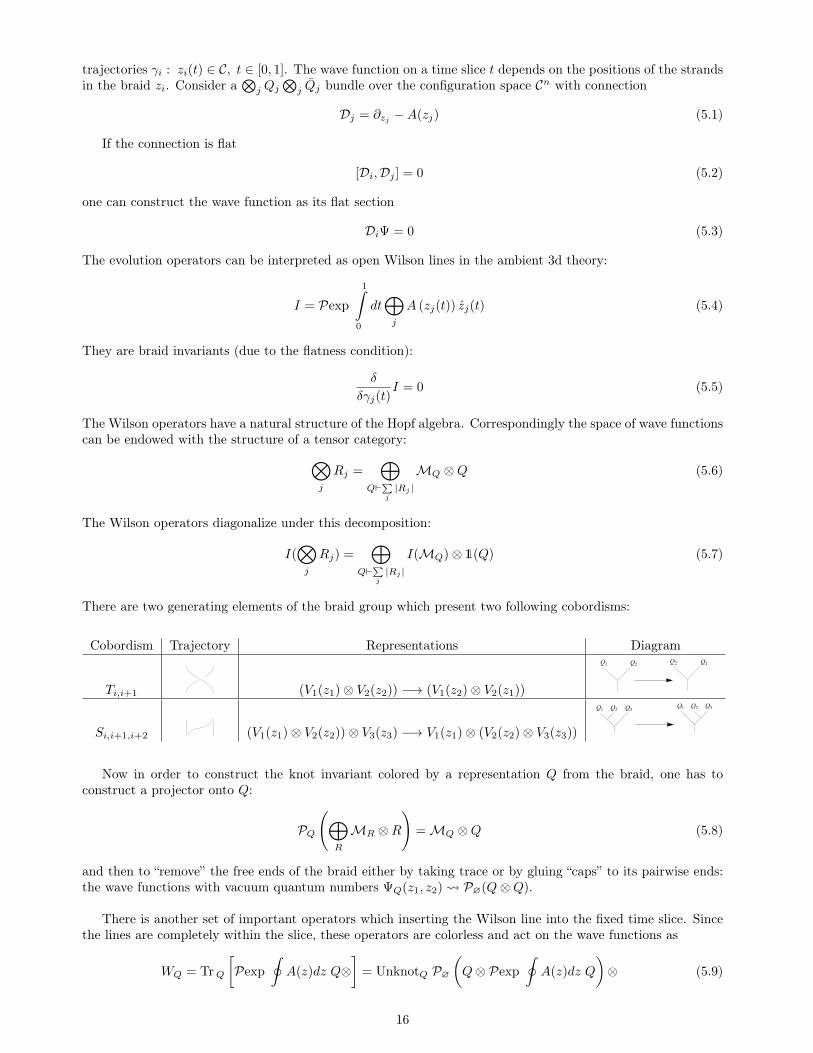
There are two generating elements of the braid group which present two following cobordisms:

Cobordism Trajectory Representations Diagram

Ti,i+1 (V1(z1)⊗ V2(z2)) −→ (V1(z2)⊗ V2(z1))

Q1Q1Q2

Q2

Si,i+1,i+2 (V1(z1)⊗ V2(z2))⊗ V3(z3) −→ V1(z1)⊗ (V2(z2)⊗ V3(z3))

Q1Q1Q2

Q2Q3Q3

Now in order to construct the knot invariant colored by a representation Q from the braid, one has toconstruct a projector onto Q:

PQ

(⊕R

MR ⊗R

)=MQ ⊗Q (5.8)

and then to “remove” the free ends of the braid either by taking trace or by gluing “caps” to its pairwise ends:the wave functions with vacuum quantum numbers ΨQ(z1, z2) P∅(Q⊗Q).

There is another set of important operators which inserting the Wilson line into the fixed time slice. Sincethe lines are completely within the slice, these operators are colorless and act on the wave functions as

WQ = TrQ

[Pexp

∮A(z)dz Q⊗

]= UnknotQ P∅

(Q⊗ Pexp

∮A(z)dz Q

)⊗ (5.9)

16

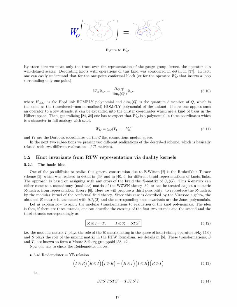
Figure 6: WQ

By trace here we mean only the trace over the representation of the gauge group, hence, the operator is awell-defined scalar. Decorating knots with operations of this kind was considered in detail in [37]. In fact,one can easily understand that for the one-point conformal block (or for the operator WQ that inserts a loopsurrounding only one point)

WQΨQ′ =HQ,Q′

dimq(Q′)ΨQ′ (5.10)

where HQ,Q′ is the Hopf link HOMFLY polynomial and dimq(Q) is the quantum dimension of Q, which isthe same as the (unreduced=non-normalized) HOMFLY polynomial of the unknot. If now one applies suchan operator to a few strands, it can be expanded into the cluster coordinates which are a kind of basis in theHilbert space. Then, generalizing [24, 38] one has to expect that WQ is a polynomial in these coordinates whichis a character in full analogy with s.4.4,

WQ = χQ(Y1, . . . , Yk) (5.11)

and Yk are the Darboux coordinates on the C flat connections moduli space.In the next two subsections we present two different realizations of the described scheme, which is basically

related with two different realizations of R-matrices.

5.2 Knot invariants from RTW representation via duality kernels5.2.1 The basic idea

One of the possibilities to realize this general construction due to E.Witten [2] is the Reshetikhin-Turaevscheme [3], which was realized in detail in [39] and in [40, 6] for different braid representations of knots/links.The approach is based on assigning with any cross of the braid the R-matrix of Uq(G). This R-matrix caneither come as a monodromy (modular) matrix of the WZWN theory [39] or can be treated as just a numericR-matrix from representation theory [6]. Here we will propose a third possibility: to reproduce the R-matrixby the modular kernel of the conformal field theory. Since this case is described by the Virasoro algebra, theobtained R-matrix is associated with SUq(2) and the corresponding knot invariants are the Jones polynomials.

Let us explain how to apply the modular transformations to evaluation of the knot polynomials. The ideais that, if there are three strands, one can describe the crossing of the first two strands and the second and thethird strands correspondingly as

R⊗ I = T, I ⊗R = STS† (5.12)

i.e. the modular matrix T plays the role of the R-matrix acting in the space of intertwining operatorsMQ (5.6)and S plays the role of the mixing matrix in the RTW formalism, see details in [6]. These transformations, Sand T , are known to form a Moore-Seiberg grouppoid [58, 42].

Now one has to check the Reidemeister moves:

• 3-rd Reidemeister = YB relation(I ⊗R

)(R⊗ I

)(I ⊗R

)=(R⊗ I

)(I ⊗R

)(R⊗ I

)(5.13)

i.e.

STS†TSTS† = TSTS†T (5.14)

17

is solved by the anzatz

SS† = 1,

STS†TST = I (5.15)

because it can be rewritten as(STS†TST

)S† = T

(STS†TST

)T−1S−1 (5.16)

In the simplest situation (the four-point spherical conformal block) we additionally have S† = S, andtherefore (5.15) reduce to

S2 = 1 and (ST )3 = 1 (5.17)

• 2-nd Reidemeister: TT−1 = 1

• 1-st Reidemeister:

T ijklPki = P jl (5.18)

where P is the cap projector.

The simplest non-trivial solution to (5.17) is in 2×2 matrices. If T is diagonalized, then S is the elementarymixing matrix of [6]:

T =

q 0

0 − 1q

, S =

1[2]

√[3]

[2]

√[3]

[2] − 1[2]

(5.19)

where quantum numbers [2] = q + q−1 and [3] = q2 + 1 + q−2.

5.2.2 S in (5.19) as the Racah matrix

Consider the representation-product diagrams from [6] for the particular choice of external legs:

@@

@@

@@@

@

@@

[1] [1]

[1] [1] [1] [1] [1] [1]

i J=

∑J SiJ

[1] [1]

[1] [1]

Both sets of intermediate states are 2-dimensional, but different: i = [2], [11] and J = 0, Adj, i.e. J =[0], [21N−1]. Note also that the conjugate fundamental representation [1] = [1N−1]. For N = 2 there arecoincidences: [1] = [1], Adj = [2], [11] = [0], therefore the two diagrams are the same, moreover the matrix SiJcoincides with that for the Racah matrix for [1]⊗3 −→ [1], which is known from ref.[6] to be exactly (5.19).

5.2.3 S and T matrices from conformal theory

Instead of trying to find solutions to eqs.(5.17) within the group theory framework, one can use anotherpossibility: the same equations are solved by the modular kernels that control modular transformations of theconformal blocks. In the generic case, these transformations are given by integral kernels. However, in thecase degenerate fields they become matrices. Since the Virasoro algebra is associated with SU(2), one expectsobtained in this way the S- and T -matrices to generate the colored Jones polynomials, while going furtherto SU(N) with N > 2 would require modular transformations of the conformal blocks of the correspondingWN -algebras.

18

Thus, we are going to consider the conformal blocks with the fields Φ(m,n) degenerate at level m · n whichhave conformal dimensions [41]

∆(m,n) = α(m,n)

(α(m,n) − b+

1

b

), α(m,n) =

1

2

(m− 1

b− (n− 1)b

)(5.20)

and b parameterizes the central charge of conformal theory: c = 1 − 6(b − 1/b)2. At the same time, choosingdifferent n changes the spin of representation (of the colored Jones polynomial).

Now we are going to read off the matrix S from the modular transformation

Bjs

[j2 j3j1 j4

](x) =

∑jt

Sjs jt

[j2 j3j1 j4

]Bjt

[j2 j1j3 j4

](1− x) (5.21)

The fundamental representation. Let us consider the simplest example of the fundamental representationof SU(2). In this case, one may expect that the end of the Wilson line in the fundamental representation [1]behaves as Φ(1,2) in the conformal theory

Φ(1,2) ⊗ Φ(1,2) = Φ(1,3) ⊕ Φ(1,1) (5.22)

Then, one has (where index means a projection in the intermediate channel on the corresponding state)

B[11](x) =⟨Φ(1,2)(0)Φ(1,2)(x)

∣∣(1,1)

Φ(1,2)(1)Φ(1,2)(∞)⟩

= xδ(1− x)δ2F1

[α, βγ

](x), (5.23)

B[2](x) =⟨Φ(1,2)(0)Φ(1,2)(x)

∣∣(1,3)

Φ(1,2)(1)Φ(1,2)(∞)⟩

= xδ(1− x)δ2F1

[α− γ + 1, β − γ + 1

2− γ

](x) (5.24)

where

α =3

2b2+

7

2, β =

1

2b2+

3

2, γ =

1

b2+ 3, δ =

3b2

4+

1

4b2+

3

2, δ =

3b2

4− 3

4b2− 1

2(5.25)

Then, the matrix S reads in this case (S2 = 1)

S =

Γ(2+ 2b2

)Γ(− 2b2−1)

Γ(1+ 1b2

)Γ(− 1b2

)Γ(2+ 2

b2)Γ( 2

b2+1)

Γ(1+ 1b2

)Γ( 3b2

+2)Γ(− 2

b2)Γ(− 2

b2−1)

Γ(− 1b2

)Γ(− 3b2−1)

Γ(− 2b2

)Γ( 2b2

+1)Γ(− 1

b2)Γ( 1

b2+1)

= eiπ

1[2]

√[3]

[2] γ2

√[3]

[2] γ−2 − 1

[2]

= U ·

1[2]

√[3]

[2]√[3]

[2] − 1[2]

· U−1(5.26)

where

γ2 = (2 + b2)[2]√[3]

Γ2(1 + 2

b2

)Γ(

1b2

)Γ(

2 + 3b2

) (5.27)

and

U = eiπ2

(γ 00 γ−1

)(5.28)

while the matrix T is2 ((ST )3 ∼ 1)

T ∼(q 00 − 1

q

)(5.29)

The overall normalization of the matrix T is an inessential overall state space phase, it can be fixed from therequirement (ST )3 = 1. When checking various relations here, we used

Γ(z)Γ(1− z) =π

sinπz, cos(παb−2) =

qα + q−α

2, sin(παb−2) =

qα − q−α

2i(5.30)

Note that this matrix S differs from that in (5.19) by the additional U -conjugation (5.28). However, thisconjugation influences neither on the relation (ST )3 = 1, nor on S2 = 1, and does not change the answers forthe knot polynomials.

2In this section q = eπib−2

.

19

Higher spin representations. So far we considered only the fundamental representation of SU(2). Similarly,one can consider representations of higher spins. To this end, one has to use Φ(1,2)⊗Φ(1,2)⊗Φ(1,s+1)⊗Φ(1,s+1)

with the fusion matrices

S =

Γ(2+ 2b2

)Γ(− s+2

b2+ 1b2−1)

Γ(1+ 1b2

)Γ(− s+2

b2+ 2b2

)Γ(2+ 2

b2)Γ( s+2

b2− 1b2

+1)Γ(1+ 1

b2)Γ( s+2

b2+2)

Γ(− 2b2

)Γ(− s+2

b2+ 1b2−1)

Γ(− 1b2

)Γ(− s+2

b2−1)

Γ(− 2b2

)Γ( s+2

b2− 1b2

+1)Γ(− 1

b2)Γ( s+2

b2− 2b2

+1)

(5.31)

T =

(qs+12 e

iπ2 0

0 q−s+12 e−

iπ2

)(5.32)

These matrices can be obtained either directly from the equations for the degenerate conformal fields, or fromthe general expression for the modular kernel due to B.Ponsot and J.Teschner [42]. This latter procedure isdiscussed in the Appendix.

Using these S and T matrices, one can easily generate the Jones polynomials as it was explained above.Note that one can easily construct the most generic modular kernel S, when the only field is degenerate at thesecond level: the general degenerate conformal block with j2 = 1 is described by the hypergeometric function

B(x) ∼ 2F1

[2 + b−2

2 (3 + j1 + j3 + j4) 1 + b−2

2 (1 + j1 + j3 − j4)2 + b−2(1 + j1)

](x) (5.33)

The corresponding monodromy matrix reads3

S(j1, 1, j3, j4) =

Γ( j1+1

b2+2)Γ

(− b

2+j3+1

b2

)Γ(

2b2+j1−j3+j4+1

2b2

)Γ(− 1−j1+j3+j4

2b2)

Γ( j1+1

b2+2)Γ

(b2+j3+1

b2

)Γ(

2b2+j1+j3−j4+1

2b2

)Γ(

4b2+j1+j3+j4+3

2b2

)Γ(− j1+1

b2)Γ

(− b

2+j3+1

b2

)Γ(− j1+j3−j4+1

2b2)Γ(− 2b2+j1+j3+j4+3

2b2

) Γ(− j1+1

b2)Γ

(b2+j3+1

b2

)Γ(− j1−j3+j4+1

2b2)Γ(

2b2−j1+j3+j4+1

2b2

)

(5.35)

The higher spin matrix is generated from the recursion formula derived [43] from the “cabling” procedure([r]⊗ [1] = [r + 1]⊕ [r − 1]):

Sq,q′

[r + 1 j3j1 j4

]=∑s,p

Sr+1,s

[1 qr j1

]Sq,p

[1 j3s j4

]Ss,q′

[r pj1 j4

]Sp,r+1

[r 1q′ j3

](5.36)

5.2.4 Plat representation of link diagrams (spherical conformal block)

Since operators S and T , satisfying (5.15) naturally arise as modular transformations of conformal blocks,one can associate them with the link diagrams in the plat representation in the following way.

We begin with examples.

1 cap There is nothing to consider in the case of one cap: independently of the number of interweavingsbetween two strands, it is always the unknot:

(Tn)22 = (−q)−n (5.37)

2 caps Our notation should be clear from the picture, where the bottom pictures present the conformalblock one starts with, the middle pictures present the monodromy of points in the conformal block and the toppictures present the resulting conformal block:

3To be precise, this matrix is related to the modular kernel as

Sjs jt

[1 j3j1 j4

]=

∑h,h′=±1

δ(js − j1 − h)δ(jt − j3 − h′)S(j1, 1, j3, j4)h,h′ (5.34)

20

?6

?6

HH

HH

0

HH

HH

0U

?6

?6

HH

HH

0

HH

HH

j

r1 r1 r2 r2

r1

r1 r2

r2

r1 r1 r2 r2

r1

r1 r2

r2

r1

r1 r2

r2

⊕j

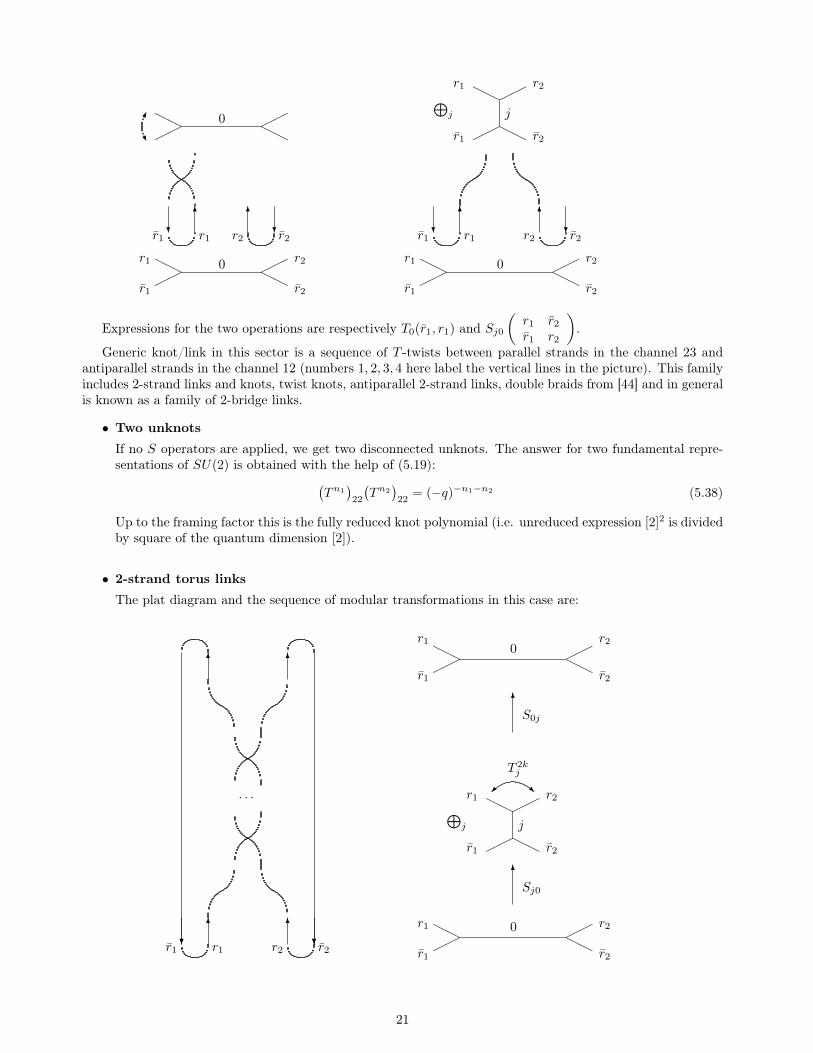
Expressions for the two operations are respectively T0(r1, r1) and Sj0(r1 r2

r1 r2

).

Generic knot/link in this sector is a sequence of T -twists between parallel strands in the channel 23 andantiparallel strands in the channel 12 (numbers 1, 2, 3, 4 here label the vertical lines in the picture). This familyincludes 2-strand links and knots, twist knots, antiparallel 2-strand links, double braids from [44] and in generalis known as a family of 2-bridge links.

• Two unknots

If no S operators are applied, we get two disconnected unknots. The answer for two fundamental repre-sentations of SU(2) is obtained with the help of (5.19):(

Tn1)

22

(Tn2

)22

= (−q)−n1−n2 (5.38)

Up to the framing factor this is the fully reduced knot polynomial (i.e. unreduced expression [2]2 is dividedby square of the quantum dimension [2]).

• 2-strand torus links

The plat diagram and the sequence of modular transformations in this case are:

?6

?6

. . .

?

6

?

6

HH

HH

0

HH

HH

0

HH

HH

j

R

T 2kj

r1 r1 r2 r2 r1

r1 r2

r2

r1

r1 r2

r2

⊕j

r1

r1 r2

r2

6

6

Sj0

S0j

21

The corresponding analytical expression is∑j

S0j

[r1 r2

r1 r2

]Tj[r1, r2

]2kSj0

[r1 r2

r1 r2

](5.39)

In the case of two fundamental representations, r1 = r2 = [1] of SU(2), one can use matrices (5.19) andobtain:

ST 2kS(5.19)

=1

[2]2

q2k + q−2k[3](q2k − q−2k

)√[3](

q2k − q−2k)√

[3] q2k[3] + q−2k

(5.40)

Expression in the right lower corner (the matrix element 22) is exactly the reduced Jones polynomial

J[2,2k][1],[1] =

1

[N ]2

(q2k [N ][N + 1]

[2]+ q−2k [N ][N − 1]

[2]

)∣∣∣∣N=2

=1

[2]2

([3]q2k + q−2k

)(5.41)

for the 2-strand torus links (in the Rosso-Jones framing [45]).

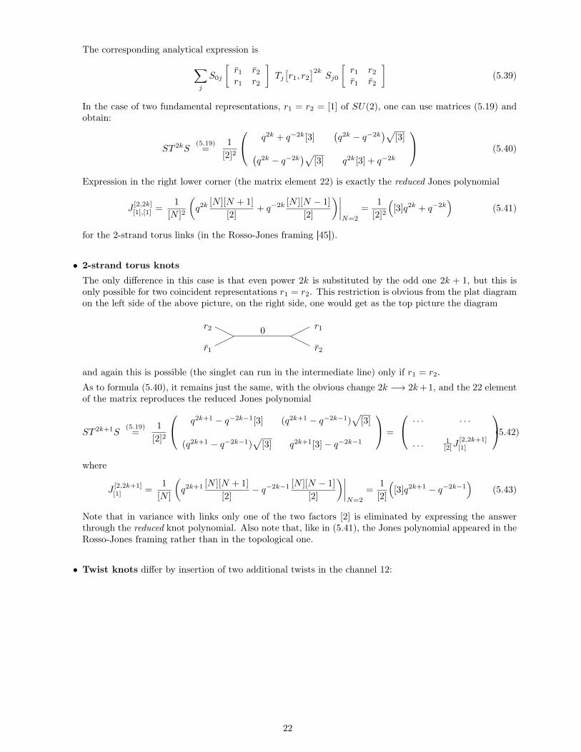
• 2-strand torus knots

The only difference in this case is that even power 2k is substituted by the odd one 2k + 1, but this isonly possible for two coincident representations r1 = r2. This restriction is obvious from the plat diagramon the left side of the above picture, on the right side, one would get as the top picture the diagram

HH

HH

0

r1

r2 r1

r2

and again this is possible (the singlet can run in the intermediate line) only if r1 = r2.

As to formula (5.40), it remains just the same, with the obvious change 2k −→ 2k+ 1, and the 22 elementof the matrix reproduces the reduced Jones polynomial

ST 2k+1S(5.19)

=1

[2]2

q2k+1 − q−2k−1[3] (q2k+1 − q−2k−1)√

[3]

(q2k+1 − q−2k−1)√

[3] q2k+1[3]− q−2k−1

=

. . . . . .

. . . 1[2]J

[2,2k+1][1]

(5.42)where

J[2,2k+1][1] =

1

[N ]

(q2k+1 [N ][N + 1]

[2]− q−2k−1 [N ][N − 1]

[2]

)∣∣∣∣N=2

=1

[2]

([3]q2k+1 − q−2k−1

)(5.43)

Note that in variance with links only one of the two factors [2] is eliminated by expressing the answerthrough the reduced knot polynomial. Also note that, like in (5.41), the Jones polynomial appeared in theRosso-Jones framing rather than in the topological one.

• Twist knots differ by insertion of two additional twists in the channel 12:

22

?6

?6

. . .

?6

?

?HH

HH

0

HH

HH

lU

T 2l

⊕l

HH

HH

j

R

T 2kj

HH

HH

0

r r r r r

r r

r

r

r r

r

⊕j

r

r r

r

r

r r

r

6

6

6

Sj0

Slj

S0l

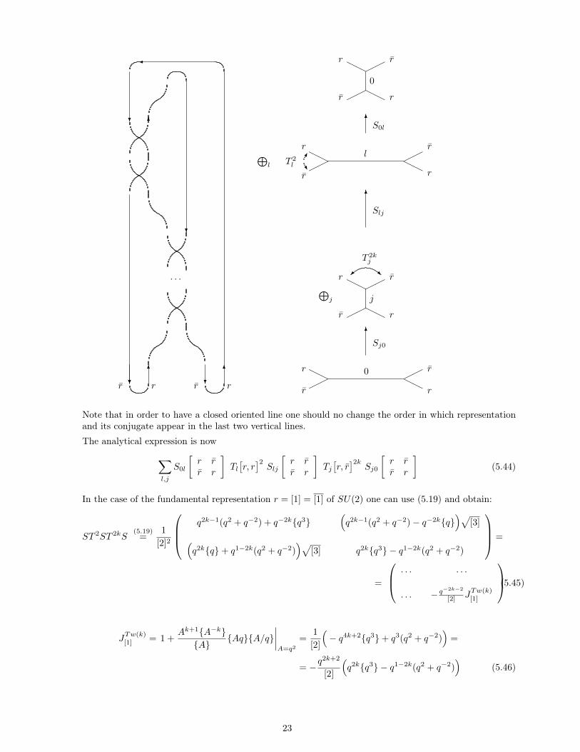
Note that in order to have a closed oriented line one should no change the order in which representationand its conjugate appear in the last two vertical lines.

The analytical expression is now∑l,j

S0l

[r rr r

]Tl[r, r]2Slj

[r rr r

]Tj[r, r]2k

Sj0

[r rr r

](5.44)

In the case of the fundamental representation r = [1] = [1] of SU(2) one can use (5.19) and obtain:

ST 2ST 2kS(5.19)

=1

[2]2

q2k−1(q2 + q−2) + q−2kq3

(q2k−1(q2 + q−2)− q−2kq

)√[3]

(q2kq+ q1−2k(q2 + q−2)

)√[3] q2kq3 − q1−2k(q2 + q−2)

=

=

. . . . . .

. . . − q−2k−2

[2] JTw(k)[1]

(5.45)

JTw(k)[1] = 1 +

Ak+1A−kA

AqA/q∣∣∣∣A=q2

=1

[2]

(− q4k+2q3+ q3(q2 + q−2)

)=

= −q2k+2

[2]

(q2kq3 − q1−2k(q2 + q−2)

)(5.46)

23

3 caps The initial state in this case can be represented as

?6

?6

?6

HH

HH

HH

0 0

0

This picture shows one of the possible mutual orientations of the three lines, which is suitable for thefollowing example. One can now make the chain of modular transformations (from the above 2-cap examplesit should be clear what is the associated link diagram, but analytical expressions can be read from the chain ofmodular transformations):

HH

HH

AA

0 0

0H

H

HHAA

0 0

j

HH

HH

HH

AA

jk l

HHHH

HH

A

A

k l

m

-Sj0

?

Sk0 ⊗ Sl0

Smj

Now one can apply T transformations in any of the channels, moving back and forth along this chain.The typical analytical expression begins from:

. . . Tm[r, r]aSmj

[k lt r

]Tk[r, r]bTl[r, r]cSl0

[r rj r

]Sk0

[r rr j

]Sj0

[r r0 0

](5.47)

As usual, it is read from right to left, and one can add arbitrary many S transforms and their conjugate of thesame type to the left.

Note that the obvious selection rule dictates that j = r, thus actually there is no sum involving arguments(not just indices) of the matrix S. However, such sums can appear after additional applications of S.

5.3 Hikami knot invariants from check-operatorsThere is another, alternative construction of R-matrices, which has a geometric origin and is associated with

tetrahedra volume [46, 47, 48, 49]. It is basically associated with Chern-Simons theory with a complex gaugegroup GC [50].

5.3.1 Quantum spectral curve in Chern-Simons theory

The Chern-Simons theory on a 3d manifold M with a complex gauge group SL(2,C) is defined by thefollowing action [51]

S(A, A) =t+8π

∫M

Tr

(A ∧ dA+

2

3A ∧A ∧A

)+t−8π

∫M

Tr

(A ∧ dA+

2

3A ∧ A ∧ A

)(5.48)

where

t± = k ± is, k ∈ Z, s ∈ R (5.49)

24

and the path integral runs over both A and A:∫DADA eiS(A,A) (5.50)

Here we are going to deal with correlation functions of only fields A. Since we are interested in constructingknot polynomials in this theory, i.e. the Wilson averages, we follow the logic of s.5.1: consider a monodromyof the wave function as a time evolution. We consider the case when C is represented by a sphere and thegauge group is SL(2,C). Fixing the representations along the Wilson lines, one can represent the average ofthe Wilson lines that begin at points vi and finish at points xi as the tensor

ρ

⟨⊗i

Pexp

xi∫vi

A

⟩ =⊗i

ρi(g(xi))⊗j

ρj(g−1(xj))Ψ(x1, . . . , xn, v1, . . . , vn) (5.51)

The tensor-valued wave function Ψ here is a conformal block of the WZWN theory, which satisfies the Knizhnik-Zamolodchikov equation with respect to the both sets of variables vi and xi:

(t+ − 2)∂xiΨ =∑j 6=i

ρi(τa)⊗ ρj(τa)

xi − xjΨ (5.52)

Let one of the representations be fundamental and denote the corresponding end-point as z, while the remainingones are xi. Then,

(t+ − 2)∂zΨ = Φ(z)Ψ, Φ(z) :=∑i

σa ⊗ ρi(τa)

z − xi (5.53)

where σa are the Pauli matrices. The equation for the first component Ψ1 is

~∂2zΨ1 = Φ11∂z log

(Φ11

Φ12

)·Ψ1 + ~∂z log Φ12 · ∂zΨ1 +

1

~

(Φ2)

11·Ψ1 (5.54)

with ~ = t+− 2. In the quasiclassical limit, only the last term at the r.h.s. of this equation survives so that onefinally obtains

~∂2zΨ1 =

∑i

c2(ρi)

(z − xi)2Ψ1 +

∑i

1

z − xi

∑j 6=i

ρi(τa)⊗ ρj(τa)

xi − xj︸ ︷︷ ︸~∂xi

Ψ1 (5.55)

with c2(ρ) being the second Casimir element. This is the spectral curve equation of the form (4.34), with thepotential parameterized by zi and, hence, the check-operator acts on zi. The potential itself can be restored fromcomparing this equation and (4.34). This similarity of (5.55) and (4.34) allows one to make “β-ensemble inter-pretations” in Chern-Simons theory. The derivative ∂z is definitely replaced in the quasiclassical approximationwith the spectral parameter λ.

5.3.2 Verlinde operators

Consider an operator that acts on the Hilbert space in Chern-Simons theory

O(R)γ : HCS → HCS (5.56)

and define from the Knizhnik-Zamolodchikov equation (5.52) an “evolution” operator that moves points of thewave function, or conformal block from their initial positions zi (the initial moment of the evolution, t = 0) tothe final positions after monodromy transformation made vi (the final moment of the evolution, t = T ):

U(Knot) :=⊗i

Pexp

∫ith strand

Aidζi =⊗i

Pexp

∫ vi

zi

dζi1

~∑j 6=i

ρi(τa)⊗ ρj(τa)

ζi − ζj(5.57)

so that one can generate knots invariants evaluating either the trace of this operator in⊗i

Ri or its projection.

In the Heisenberg representation

U(Knot)−1O(R)γ (0) U(Knot) = O(R)

γ (T ) (5.58)

25

and if one knows both O(R)γ (0) and O(R)

γ (T ), it is possible to evaluate U(Knot) from the equation

O(R)γ (0) U(Knot) = U(Knot) O(R)

γ (T ) (5.59)

Let us introduce a set of “Verlinde operators” acting on the space of conformal blocks HCS as the monodromytrace (straight analogs of WR from s.5.1):

O(R)γ := TrR Pexp

∮γ

dζ1

~∑i

~τ ⊗ ~τiζ − zi

(5.60)

They can be rewritten following “the β-ensemble interpretation” in terms of check-operators as the trace ofmonodromy:

O(R)γ = TrRe

1~∮γ

∇(5.61)

while the counterparts of monodromy itself are the (Fock-Goncharov) cluster coordinates

wγ := e1~∮γ

∇(5.62)

which form a Heisenberg algebra:

wγwγ′ = q〈γ,γ′〉wγ+γ′ (5.63)

Then, one can solve equation (5.59) in terms of this algebra:

U(Knot) = f(wγ) (5.64)

This algebra admits a realization in the space of conformal blocks [38] with manifest realization wA =ea, wB = q∂a so that the evolution operator is realized as U(Knot) = f(ea, q∂a) and reduces to a modulartransformation of the conformal block in terms of S- and T -matrices/kernels.

5.3.3 Knots and flips

Quasiclassical limit. As we described, one can associate with eachWZWN conformal block the correspondingKnizhnik-Zamolodchikov equation (and its derivative (5.55)), and with this later a WKB network. When thepoints of the conformal block are subject to monodromy transformations, this Chern-Simons evolution can bedescribed by reconstructions of the WKB network by a series of flips (mutations). In terms of the Heisenbergalgebra (5.63) associated with the Stokes lines γ’s, we reinterpret flips as an action of some evolution operatorsu on wγ , and the discretized smooth evolution is now

U(Knot) ∏

γ∈flips

uγ(X) (5.65)

Therefore, one can consider the spectral curve that emerges in the “quasiclassical” limit ~ → 0, (5.55):∇2(z) − T (z) = 0 and the Stokes lines Im ~−1∇ = 0 (see (2.2)) so that we are able to present quasiclassicalexpressions for the operators:

O(R)γ ∼

∑sheets

e

∮γ

∇+ Stokes detours (5.66)

A single flip along the edge γ is calculated as in s.2.2 and is equal (see eq.(2.12))

Flipγ(wγ′) =

wγ′ , 〈γ, γ′〉 = 0wγ′(1 + wγ), 〈γ, γ′〉 = 1

(5.67)

26

Quantization. Similarly to s.4.1, using technique presented in [20] one can calculate the quantum flip. Theresult is

Flipγ(wγ′) =

wγ′ , 〈γ, γ′〉 = 0

wγ′∏|〈γ,γ′〉|a=1

(1 + q2a−1w

〈γ,γ′〉γ

)〈γ,γ′〉, |〈γ, γ′〉| = 1

(5.68)

This flip is described by the adjoint action of uγ :

wγ′uγ(w) = uγ(w)Flipγ(wγ′) (5.69)

which means that

uγ(w) ∼ Φ(logwγ) (5.70)

where quantum dilogarithm is defined as [52]

Φ(z|τ) = exp

(−1

4

∫R+i0

dw

w

e−2iwz

sinh b−1w · sinh bw

)(5.71)

5.3.4 Hikami invariant as a KS invariant

Thus, one is able to rewrite the evolution operator U(Knot) as a product of R-matrices each of them, in itsterm, being a product of mutations:

R =:∏i

uγi : (5.72)

Having the manifest expression for uγ in terms of quantum dilogarithm (5.71), one can construct a manifestrepresentation for the R-matrix. This can be done either by using our manifest realization of the clustercoordinates (5.62), or in a more formal way [49], the answer for the R-matrix being a product of ratios ofquantum dilogarithms. In order to obtain the knot polynomial one still has to calculate the trace of a productof R-matrices.

Afterwards the R-matrix can be rewritten in terms of tensor categories after substitution of values forcluster coordinates in terms of tensor categories. From this point of view Virc and Uq(sl2) are equivalent tensorcategories [42]4.

Quasiclassical limit [48]. As was demonstrated in [48, 49], the R-matrix can be associated with an idealhyperbolic octahedron. This is not surprising since the quantum dilogarithm (5.71) in the quasiclassical limit(q → 1) is related to the hyperbolic volume of ideal tetrahedron ∆ so that the R-matrix has the asymptoticform

R ∼ e1~2

∑i

∆i

(5.73)

5.4 Stokes phenomenon in conformal blocks5.4.1 WKB approximation

As we have seen the spectral curve for a braid of n strands placed at xi reads (5.55)

λ2 =

n∑i=1

(c2(ρi)

(z − xi)2+

uiz − xi

)dz2 (5.74)

The web of WKB lines is constructed as trajectories of solutions to equation (2.2)

Im ~−1λ = 0 (5.75)

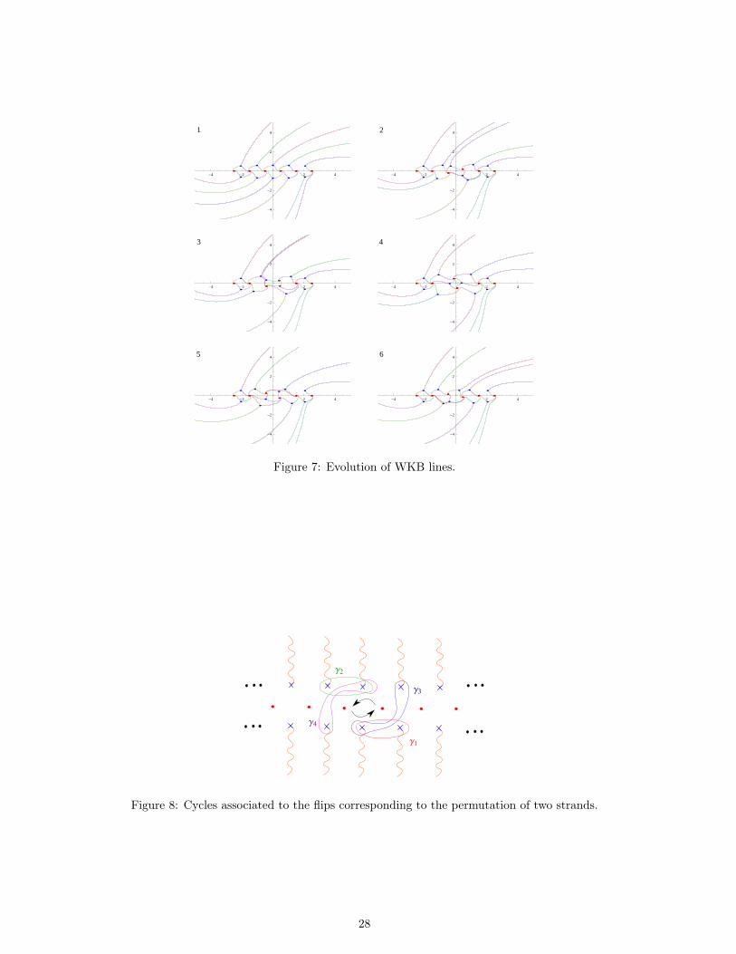
Here we present the evolution of the WKB lines for six strands associated to the premutation of two middlestrands in order to mimic the action of the R-matrix. The blue dots mark positions of zeroes of the discriminant,while the red ones mark positions of the strands (singularities of the curve).

27

1

-4 -2 2 4

-4

-2

2

4 2

-4 -2 2 4

-4

-2

2

4

3

-4 -2 2 4

-4

-2

2

4 4

-4 -2 2 4

-4

-2

2

4

5

-4 -2 2 4

-4

-2

2

4 6

-4 -2 2 4

-4

-2

2

4

Figure 7: Evolution of WKB lines.

Figure 8: Cycles associated to the flips corresponding to the permutation of two strands.

28

It is simple to observe four simple flips associated to cycles γ1, γ2, γ3, γ4 in the order as they are mentionedas it is depicted in Fig.8.

Hence, the action of the R-matrix is mimiced by the following operator (cf. with [49, eq.(3.15)])

R ∼ Φ(wγ4)Φ(wγ3)Φ(wγ2)Φ(wγ1) (5.76)

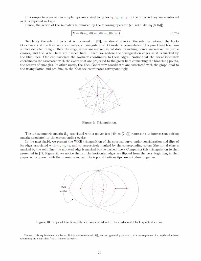
To clarify the relation to what is discussed in [49], we should mention the relation between the Fock-Goncharov and the Kashaev coordinates on triangulations. Consider a triangulation of a punctured Riemannsurface depicted in fig.9. Here the singularities are marked as red dots, branching points are marked as purplecrosses, and the WKB lines are dashed lines. Then, we restore the triangulation edges as it is marked bythe blue lines. One can associate the Kashaev coordinates to these edges. Notice that the Fock-Goncharovcoordinates are associated with the cycles that are projected to the green lines connecting the branching points,the centers of triangles. In other words, the Fock-Goncharov coordinates are associated with the graph dual tothe triangulation and are dual to the Kashaev coordinates correspondingly.

Figure 9: Triangulation.

The antisymmetric matrix Bij associated with a quiver (see [49, eq.(2.1)]) represents an intersection pairingmatrix associated to the corresponding cycles.

In the next fig.10, we present the WKB triangualtion of the spectral curve under consideration and flips ofits edges associated with γ1, γ2, γ3, and γ4 respectively marked by the corresponding colors (the initial edge ismarked by the solid line, the mutated edge is marked by the dashed line.) Comparing this triangulation to thatpresented in [49, Figure 2], we notice that all the horizontal edges are flipped from the very beginning in thatpaper as compared with the present ones, and the top and bottom tips are not glued together.

Figure 10: Flips of the triangulation associated with the conformal block spectral curve.

4Indeed this equivalence can be explicitly demonstrated [38], and on general grounds it is a consequence of a mythical mirrorsymmetry in a mythical Virq,t-tensor category.

29

6 Conclusion and DiscussionIn this short review we tried to give a simple intuitive description for various new interesting phenomena de-

scribed recently in the literature. The story includes such issues as quantum spectral curves, Teichmuller theory,cluster varieties, moduli space of flat connections, different theories produced by M5-brane compactification,etc...

Many of these subjects are related to a 2d Coulomb gas system (β-ensemble), maybe via different chains ofdualities or correspondences. The usual technique to derive correlators in the β-ensemble system, the topologicalrecursion gives rise to an infinite chain of linked equations: the loop equations. We argued that the loopequations arising within this approach are much similar to those arising within the WKB approach to solvingdifferential equations. The major modification is that in β-ensembles there are two deformation coefficients: g,a string coupling constant, and β. This can be reinterpreted in such a way that, to the usual Plank constant~ controlling WKB expansion of, say, Schrodinger equation one should add another deformation parameter~′ that will control commutation relations of eikonals. Thus, the eikonals become non-commutative operatorsacting on some modified Hilbert space, where the β-ensemble partition function behaves as a wave function onthe moduli space.

As we discussed, the main characters of this construction are: the flat connection on Riemann surface, theholonomy of this connection, the spectral parameter or eikonal, the cluster coordinates arising as holonomies ofthis eikonal, and the Hilbert space associated with the partition faction playing a role of the wave function. Aswell, many theories are tightly related to some dualities. Here we present various avatars of the same notionsemerging in different theories. Some of the avatars have been so far not discussed in the literature, hence, weleave the corresponding boxes blank:

Theory Hilbert space Flat connec-tion

holonomy spectral pa-rameter

cluster coor-dinate

duality

2d CFT conf. block T (z) Verlindeoperator[54,43]

chiralcurrent[55]

Y-functions fusion rules

β-ensembles part. func. resolvent S-dualitytop. strings part. func. U(1)-Chern-

SimonsWilson loops

Knizhnik-Zamolodchikov-Bernard

conf. block,CS wavefunction

g-connection Wilson loops Reidemeistermoves

QuantumHitchin

Landau-Ginsburgwave func.

Lax Laxholonomies

spectraldualitiesMMZZ

q-Teichmuhler wave func. spin connec-tion

spin conn.holonomies

geodesics Fock-Goncharov,Kashaev

Moore-Seiberggroupoid

Nekrasov part. func. 2d defect UV 1d defect UV 2d defect IR 1d defect IR S-duality

To complete this table with references we present the following list and web of correspondences betweendifferent theories and references:

1. 2d CFTs: [27, 28]

2. CS/topological strings: [57]

3. CS/KZB-equations: [58]

4. β-ensembles: [59]

5. Quantum integrable systems (q-Hitchin, Painleve): [60, 61]

6. R-twisted tt∗-equations: [57, 53, 19]

7. Quantum Teichmuhler theory: [62]

8. N = 2 4d theory in Ω-background: [27, 28]

30

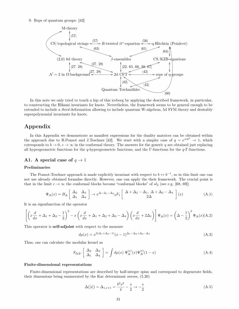
9. Reps of quantum groups: [42]

M-theoryOO

[57]

66

((

CS/topological strings oo[57] //

jj[63]

**

R-twisted tt∗-equation oo[56] // q-Hitchtin (Peinleve)

OO

[64]

RR

[60]

cc

(2,0) 6d theoryjj

[27, 28]

**

OO

[27, 28]

β-ensemblesOO

[22, 65, 66, 38, 67]

tt

[61]44

CS/KZB-equationsOO

N = 2 in Ω-background oo

[27, 28] // 2d CFT oo[42] //

tt

44

OO

[42]

reps of q-groups

Quantum Teichmuhlertt [42]

44

In this note we only tried to touch a hip of this iceberg by applying the described framework, in particular,to constructing the Hikami invariants for knots. Nevertheless, the framework seems to be general enough to beextended to include a third deformation allowing to include quantum W-algebras, 5d SYM theory and desirablysuperpolynomial invariants for knots.

AppendixIn this Appendix we demonstrate as manifest expressions for the duality matrices can be obtained within

the approach due to B.Ponsot and J.Teschner [42]. We start with a simpler case of q = eπib2 → 1, which

corresponds to b→ 0, c→∞ in the conformal theory. The answers for the generic q are obtained just replacingall hypergeometric functions for the q-hypergeometric functions, and the Γ-functions for the q-Γ-functions.

A1. A special case of q → 1

Preliminaries

The Ponsot-Teschner approach is made explicitly invariant with respect to b↔ b−1, so in this limit one cannot use already obtained formulas directly. However, one can apply the their framework. The crucial point isthat in the limit c→∞ the conformal blocks become “conformal blocks” of sl2 (see e.g. [68, 69])

Ψ∆(x) = B∆

[∆2 ∆3

∆1 ∆4

]→ x∆−∆1−∆2

2F1

[∆ + ∆2 −∆1, ∆ + ∆3 −∆4

2∆

](x) (A.1)

It is an eigenfunction of the operator[(xd

dx+ ∆1 + ∆2 −

1

2

)2

− x(xd

dx+ ∆1 + ∆2 + ∆3 −∆4

)(xd

dx+ 2∆1

)]Ψ∆(x) =

(∆− 1

2

)2

Ψ∆(x)(A.2)

This operator is self-adjoint with respect to the measure

dµ(x) = x2(∆1+∆2−1)(x− 1)∆1−∆2+∆3−∆4 (A.3)

Thus, one can calculate the modular kernel as

S∆∆′

[∆2 ∆3

∆1 ∆4

]=

∫dµ(x) Ψ

(s)∆ (x)Ψ

(t)∆′(1− x) (A.4)

Finite-dimensional representations

Finite-dimensional representations are described by half-integer spins and correspond to degenerate fields,their dimensions being enumerated by the Kac determinant zeroes, (5.20)

∆([s]) = ∆1,s+1 =b2s2

4− s

2→ −s

2(A.5)

31

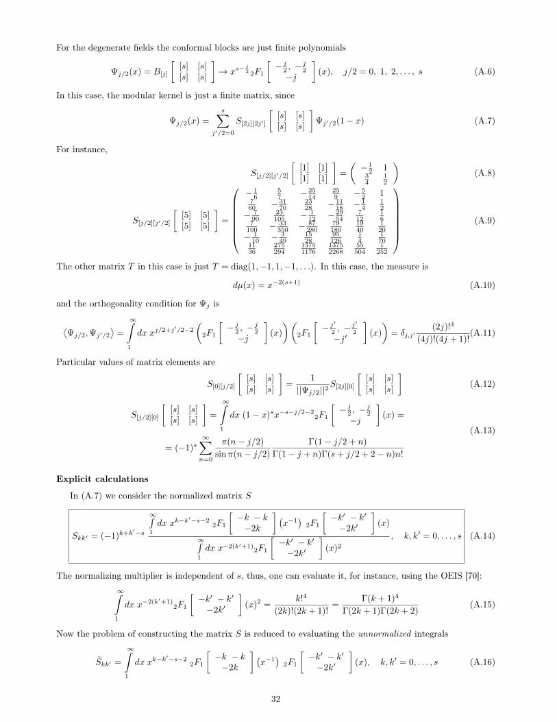
For the degenerate fields the conformal blocks are just finite polynomials

Ψj/2(x) = B[j]

[[s] [s][s] [s]

]→ xs−

j2 2F1

[− j2 , −

j2

−j

](x), j/2 = 0, 1, 2, . . . , s (A.6)

In this case, the modular kernel is just a finite matrix, since

Ψj/2(x) =

s∑j′/2=0

S[2j][2j′]

[[s] [s][s] [s]

]Ψj′/2(1− x) (A.7)

For instance,

S[j/2][j′/2]

[[1] [1][1] [1]

]=

(− 1

2 134

12

)(A.8)

S[j/2][j′/2]

[[5] [5][5] [5]

]=

− 1

657 − 25

14259 − 5

2 1760 − 31

702328 − 11

18 − 14

12

− 790

23105 − 1

12 − 2954

712

16

7100 − 33

350 − 87280

79180

1940

120

− 110 − 3

491528

95126

14

170

1136

275294

13751176

13752268

55504

1252

(A.9)

The other matrix T in this case is just T = diag(1,−1, 1,−1, . . .). In this case, the measure is

dµ(x) = x−2(s+1) (A.10)

and the orthogonality condition for Ψj is

⟨Ψj/2,Ψj′/2

⟩=

∞∫1

dx xj/2+j′/2−2

(2F1

[− j2 , −

j2

−j

](x)

)(2F1

[− j′

2 , −j′

2−j′

](x)

)= δj,j′

(2j)!4

(4j)!(4j + 1)!(A.11)

Particular values of matrix elements are

S[0][j/2]

[[s] [s][s] [s]

]=

1

||Ψj/2||2S[2j][0]

[[s] [s][s] [s]

](A.12)

S[j/2][0]

[[s] [s][s] [s]

]=

∞∫1

dx (1− x)sx−s−j/2−22F1

[− j2 , −

j2

−j

](x) =

= (−1)s∞∑n=0

π(n− j/2)

sinπ(n− j/2)

Γ(1− j/2 + n)

Γ(1− j + n)Γ(s+ j/2 + 2− n)n!

(A.13)

Explicit calculations

In (A.7) we consider the normalized matrix S

Skk′ = (−1)k+k′−s

∞∫1

dx xk−k′−s−2

2F1

[−k − k−2k

] (x−1

)2F1

[−k′ − k′−2k′

](x)

∞∫1

dx x−2(k′+1)2F1

[−k′ − k′−2k′

](x)2

, k, k′ = 0, . . . , s (A.14)

The normalizing multiplier is independent of s, thus, one can evaluate it, for instance, using the OEIS [70]:

∞∫1

dx x−2(k′+1)2F1

[−k′ − k′−2k′

](x)2 =

k!4

(2k)!(2k + 1)!=

Γ(k + 1)4

Γ(2k + 1)Γ(2k + 2)(A.15)

Now the problem of constructing the matrix S is reduced to evaluating the unnormalized integrals

Skk′ =

∞∫1

dx xk−k′−s−2

2F1

[−k − k−2k

] (x−1

)2F1

[−k′ − k′−2k′

](x), k, k′ = 0, . . . , s (A.16)

32

In this case, for instance, at s = 1

S =

1

2

1

12

3

4− 1

24

(A.17)

We use the Barnes’ integral representation for the hypergeometric function

2F1

[α βγ

](z) =

Γ(γ)

Γ(α)Γ(β)

1

2πi

i∞∫−i∞

dsΓ(α+ s)Γ(β + s)Γ(−s)

Γ(γ + s)(−z)s (A.18)

Thus

Skk′ =Γ(−2k)Γ(−2k′)

Γ(−k)2Γ(−k′)2

(1

2πi

)2i∞∫−i∞

dtΓ(t− k)2Γ(−t)

Γ(t− 2k)

i∞∫−i∞

dt′Γ(t′ − k′)2Γ(−t′)

Γ(t′ − 2k′)

∞∫1

dx xk−k′−s−2

(− 1

x

)t(−x)t

′

︸ ︷︷ ︸(−1)t+t

′

k−k′+t′−t−s−1

(A.19)

The last term gives a pole so one of the integrals can be calculated

Skk′ = (−1)k−k′−s+1 Γ(−2k)Γ(−2k′)

Γ(−k)2Γ(−k′)2

i∞∫−i∞

dt

2πi

Γ(t− k′ − s− 1)2Γ(−t− k + k′ + s+ 1)

Γ(t− k − k′ − s− 1)

Γ(t− k′)2 Γ(−t)Γ(t− 2k′)

(A.20)

The boxed term gives the poles contributing to the answer. For example,

S11 =Γ(−2)2

Γ(−1)4

(Γ(−3)2Γ(2)

Γ(−4)

Γ(−1)2

Γ(−2)− Γ(−2)2Γ(1)

Γ(−3)

Γ(0)2

Γ(−1)

)= − 1

24(A.21)

Similarly, one can calculate

Sk0 = (−1)k−sΓ(−2k)

Γ(−k)2

Γ(−s− 1)2Γ(s+ 1− k)

Γ(−s− 1− k)(A.22)

S0k = (−1)k+s+1 Γ(−2k)

Γ(−k)2

Γ(s+ 1)2Γ(−k − s− 1)

Γ(s+ 1− k)(A.23)

A2. Explicit calculations for q 6= 1

Similarly to the previous consideration

Skk′ =

∞∫1

dqx xk−k′−s−2

2φ1

[−k − k−2k

](x−1)2φ1

[−k′ − k′−2k′

](x)

∞∫1

dqx x−2(k′+1)2φ1

[−k′ − k′−2k′

](x)2

(A.24)

where

2φ1

[α βγ

](z) =

∞∑n=0

(−z)n

(n−1∏j=0

[α+ j]q

)(n−1∏j=0

[β + j]q

)(n−1∏j=0

[γ + j]q

)[n]q!

, (A.25)

[n]q =qn − q−n

q − q−1, (A.26)

∞∫1

dqx x−n =

(−1)n

[n− 1]q(A.27)

33

Formulas of the q → 1 case are generalized straightforwardly:

∞∫1

dqx x−2(k′+1)

2φ1

[−k′ − k′−2k′

](x)2 =

([k]q!)4

[2k]q! [2k + 1]q!(A.28)

and

Sk0 = (−1)k−s+1 Γq(−2k)

Γq(−k)2

Γq(−s− 1)2Γq(s+ 1− k)

Γq(−s− 1− k)(A.29)

S0k = (−1)k+s+1 Γq(−2k)

Γq(−k)2

Γq(s+ 1)2Γq(−k − s− 1)

Γq(s+ 1− k)(A.30)

where,

Γq(x+ 1) =qx − q−x

q − q−1Γq(x) (A.31)

AcknowledgementsD.G. would like to thank S.Arthamonov, P.Longhi, G.W.Moore and Sh.Shakirov for valuable and stimulating

discussions. Our work is partly supported by grant NSh-1500.2014.2, by RFBR grants 13-02-00457 (D.G. andA.Mir.), 13-02-00478 (A.Mor.), by joint grants 13-02-91371-ST, 14-01-92691-Ind, by the Brazil National Counselof Scientific and Technological Development (A.Mor.), by the program of UFRN-MCTI, Brazil (A.Mir.). Thework of D.G. is supported by the DOE under grants SC0010008, ARRA-SC0003883, DE-SC0007897.

References[1] M.Kontsevich and Y.Soibelman, arXiv:0811.2435;

See a review and further references in:B. Pioline, 1103.0261

[2] E.Witten, Comm.Math.Phys. 121 (1989) 351

[3] E.Guadagnini, M.Martellini and M.Mintchev, In Clausthal 1989, Proceedings, Quantum groups, 307-317;Phys.Lett. B235 (1990) 275;N.Yu.Reshetikhin and V.G.Turaev, Comm. Math. Phys. 127 (1990) 1-26

[4] A.Morozov and L.Vinet, Int.J.Mod.Phys. A13 (1998) 1651-1708, hep-th/9409093

[5] A.Mironov, hep-th/9409190; Theor.Math.Phys. 114 (1998) 127, q-alg/9711006

[6] A.Mironov, A.Morozov and And.Morozov, JHEP 03 (2012) 034, arXiv:1112.2654

[7] A.Morozov, Phys.Usp.(UFN) 35 (1992) 671-714; 37 (1994) 1, hep-th/9303139; hep-th/9502091; hep-th/0502010A.Mironov, Int.J.Mod.Phys. A9 (1994) 4355, hep-th/9312212; Phys.Part.Nucl. 33 (2002) 537

[8] V.V.Fock and A.B.Goncharov, Publ.Math.Inst.Hautes Etudes Sci. 103 (2006) 1-211, math/0311149

[9] S.Fomin and A.Zelevinsky, A.Amer.Math.Soc. 15 (2002) 497-529, math/0104151; Composito Math. 143(2007) 112-164, math/0602259;S.Fomin, M.Shapiro and D.Thurston, Acta Math. 201 (2008) 83-146, math/0608367;S.Fomin and D.Thurston, arXiv:1210.5569 [math.GT]

[10] A.Popolitov, arXiv:1403.1834

[11] N.Seiberg and E.Witten, Nucl.Phys., B426 (1994) 19-52, hep-th/9408099; Nucl.Phys., B431 (1994) 484-550, hep-th/9407087

[12] E.Witten, Nucl.Phys. B500 (1997) 3-42, arXiv:hep-th/9703166

34

[13] A.Mikhailov, Nucl.Phys. B533 (1998) 243-274, hep-th/9708068

[14] A.Gorsky, I.Krichever, A.Marshakov, A.Mironov and A.Morozov, Phys.Lett. B355 (1995) 466-477, hep-th/9505035;R.Donagi and E.Witten, Nucl.Phys., B460 (1996) 299-334, hep-th/9510101;H.Itoyama and A.Morozov, Nucl.Phys., B477 (1996) 855-877, hep-th/9511125; Nucl.Phys., B491 (1997)529-573, hep-th/9512161;See a review in:A.Gorsky and A.Mironov, hep-th/0011197

[15] G.F.Bonini, A.G.Cohen, C.Rebbi and V.A.Rubakov, Phys.Rev. D60 (1999) 076004, arXiv:hep-ph/9901226

[16] A.Alexandrov, A.Mironov and A.Morozov, Int.J.Mod.Phys. A19 (2004) 4127, hep-th/0310113;Teor.Mat.Fiz. 150 (2007) 179-192, hep-th/0605171

[17] A.Alexandrov, A.Mironov and A.Morozov, Int.J.Mod.Phys. A21 (2006) 2481-2518, hep-th/0412099

[18] A.Alexandrov, A.Mironov and A.Morozov, Fortsch.Phys. 53 (2005) 512-521, hep-th/0412205

[19] D.Gaiotto, G.W.Moore and A.Neitzke, arXiv:0907.3987

[20] D.Galakhov, P.Longhi and G.W.Moore, arXiv:1408.0207

[21] N.Nekrasov and S.Shatashvili, arXiv:0908.4052

[22] A.Mironov, A.Morozov, Sh.Shakirov, JHEP 02 (2010) 030, arXiv:0911.5721

[23] A.Mironov and A.Morozov, JHEP 04 (2010) 040, arXiv:0910.5670; J.Phys. A43 (2010) 195401,arXiv:0911.2396

[24] A.Marshakov, A.Mironov and A.Morozov, J.Geom.Phys. 61 (2011) 1203-1222, arXiv:1011.4491

[25] N.Nekrasov, A.Rosly and S.Shatashvili, Nucl.Phys. (Suppl.) B216 (2011) 69-93, arXiv:1103.3919

[26] D.Krefl, arXiv:1311.0584; arXiv:1410.7116

[27] L.Alday, D.Gaiotto and Y.Tachikawa, Lett.Math.Phys. 91 (2010) 167-197, arXiv:0906.3219

[28] N.Wyllard, JHEP 0911 (2009) 002, arXiv:0907.2189;A.Mironov and A.Morozov, Phys.Lett. B680 (2009) 188-194, arXiv:0908.2190; Nucl.Phys. B825 (2009)1-37, arXiv:0908.2569

[29] A. Gerasimov, A. Marshakov, A. Mironov, A. Morozov, and A. Orlov, Nucl. Phys. B357 (1991) 565-618;S.Kharchev, A.Marshakov, A.Mironov, A.Orlov and A.Zabrodin, Nucl.Phys., B366 (1991) 569-601

[30] A.Marshakov, A.Mironov, and A.Morozov, Phys.Lett. B265 (1991) 99S.Kharchev, A.Marshakov, A.Mironov, A.Morozov and S.Pakuliak, Nucl.Phys. B404 (1993) 17-750,arXiv:hep-th/9208044

[31] A.Gerasimov, S.Khoroshkin, D.Lebedev, A.Mironov, and A.Morozov, Int.J.Mod.Phys. A10 (1995) 2589-2614, hep-th/9405011

[32] A.Alexandrov, A.Mironov and A.Morozov, PhysicaD235 (2007) 126-167, hep-th/0608228; JHEP 12 (2009)053, arXiv:0906.3305

[33] N.Nekrasov, V.Pestun and S.Shatashvili, arXiv:1312.6689

[34] S.-S.Chern and J.Simons, Ann.Math. 99 (1974) 48-69

[35] J.Wess and B.Zumino, Phys.Lett. B37 (1971) 95;S.Novikov, UMN, 37 (1982) 37;E.Witten, Comm.Math.Phys. 92 (1984) 455;A.Gerasimov, A.Marshakov, A.Morozov, M.Olshanetsky, S. Shatashvili, Int.J.Mod.Phys. A5 (1990) 2495-2589

[36] V.Knizhnik and A.Zamolodchikov, Nucl.Phys. B247 (1984) 83-103

35

[37] H.Morton and S.Lukac, J. Knot Theory and Its Ramifications, 12 (2003) 395, math.GT/0108011

[38] D.Galakhov, A.Mironov and A.Morozov, JHEP 06 (2014) 050, arXiv:1311.7069

[39] R.K.Kaul and T.R.Govindarajan, Nucl.Phys. B380 (1992) 293-336, hep-th/9111063;P.Ramadevi, T.R.Govindarajan and R.K.Kaul, Nucl.Phys. B402 (1993) 548-566, hep-th/9212110;Nucl.Phys. B422 (1994) 291-306, hep-th/9312215;P.Ramadevi and T.Sarkar, Nucl.Phys. B600 (2001) 487-511, hep-th/0009188;Zodinmawia and P.Ramadevi, arXiv:1107.3918; arXiv:1209.1346

[40] A.Mironov, A.Morozov and An.Morozov, Strings, Gauge Fields, and the Geometry Behind: The Legacy ofMaximilian Kreuzer, World Scietific Publishins Co.Pte.Ltd. 2013, pp.101-118, arXiv:1112.5754;H.Itoyama, A.Mironov, A.Morozov, And.Morozov, Int.J.Mod.Phys. A27 (2012) 1250099, arXiv:1204.4785;A.Anokhina, A.Mironov, A.Morozov and And.Morozov, Nucl.Phys. B868 (2013) 271-313, arXiv:1207.0279;H.Itoyama, A.Mironov, A.Morozov, And.Morozov, Int.J.Mod.Phys. A28 (2013) 1340009, arXiv:1209.6304;A.Anokhina, A.Mironov, A.Morozov and And.Morozov, arXiv:1304.1486;A.Anokhina and An.Morozov, arXiv:1307.2216

[41] A.Belavin, A.Polyakov, A.Zamolodchikov, Nucl.Phys. B241 (1984) 333-380

[42] B.Ponsot and J.Teschner, arXiv:hep-th/9911110;B.Ponsot and J.Teschner, Commun.Math.Phys. 224 (2001) 613-655, arXiv:math/0007097

[43] N.Drukker, J.Gomis, T.Okuda and J.Teschner, JHEP 1002 (2010) 057, arXiv:0909.1105

[44] A.Mironov, A.Morozov and An.Morozov, AIP Conf. Proc. 1562 (2013) 123, arXiv:1306.3197

[45] M. Rosso and V. F. R. Jones, J. Knot Theory Ramifications, 2 (1993) 97-112;X.-S.Lin and H.Zheng, Trans. Amer. Math. Soc. 362 (2010) 1-18 math/0601267;S.Stevan, Annales Henri Poincare, 11 (2010) 1201-1224, arXiv: 1003.2861

[46] R.Kashaev, Mod.Phys.Lett. A39 (1997) 269-275

[47] K.Hikami, Int.J.Mod.Phys. A16 (2001) 3309-3333, math-ph/0105039; J.Geom.Phys. 57 (2007) 1895-1940,math/0604094

[48] K.Hikami and R.Inoue, arXiv:1212.6042, arXiv:1304.4776

[49] K.Hikami and R.Inoue, arXiv:1404.2009

[50] T.Dimofte, S.Gukov, J.Lenells and D.Zagier, Commun.Num.Theor.Phys. 3 (2009) 363-443, arXiv:0903.2472

[51] E.Witten, arXiv:1001.2933

[52] L.Faddeev and R.Kashaev, Mod.Phys.Lett. 9 (1994), 265-282, hep-th/9310070;L.Faddeev, Lett.Math.Phys. 34 (1995) 249-254, hep-th/9504111

[53] D.Gaiotto, G.W.Moore and A.Neitzke, arXiv:0807.4723, arXiv:1006.0146, arXiv:1103.2598,arXiv:1204.4824

[54] L.F.Alday, D.Gaiotto, S.Gukov, Y.Tachikawa and H.Verlinde, JHEP 1001 (2010) 113, arXiv:0909.0945;D.Gaiotto, arXiv:1404.0332

[55] L.Chekhov, B.Eynard and S.Ribault, J. Math. Phys. 54 (2013) 022306, arXiv:1209.3984

[56] S.Cecotti, D.Gaiotto and C.Vafa, arXiv:1312.1008

[57] S.Cecotti, A.Neitzke and C.Vafa, arXiv:1006.3435

[58] G.W.Moore and N.Seiberg, Lectures on RCFT, Strings’89, http://www.physics.rutgers.edu/~gmoore/LecturesRCFT.pdf

36

[59] P.Di Francesco, M.Gaudin, C.Itzykson and F.Lesage, Int.J.Mod.Phys. A9 (1994) 4257-4352, hep-th/9401163;A.Zabrodin, arXiv:0907.4929;A.Morozov and Sh.Shakirov, arXiv:1004.2917;A.Mironov, A.Morozov, A.Popolitov and Sh.Shakirov, Theor.Math.Phys. 171 (2012) 505-522,arXiv:1103.5470;A.Morozov, arXiv:1201.459;A.Mironov, A.Morozov and Z.Zakirova, Phys.Lett. B711 (2012) 332-335, arXiv:1202.6029

[60] N.Iorgov, O.Lisovyy and Yu.Tykhyy, JHEP 12 (2013) 029, arXiv:1308.4092;N.Iorgov, O.Lisovyy and J.Teschner, arXiv:1401.6104

[61] A.Mironov, A.Morozov, Y.Zenkevich, and A.Zotov, JETP Letters, 97 (2013) 45Џ51, arXiv:1204.0913;A.Mironov, A.Morozov, B.Runov, Y.Zenkevich, and A.Zotov, Letters in Mathematical Physics, 103 (2013)299Џ329, arXiv:1206.6349; JHEP 2013 (2013) 34, arXiv:1307.1502

[62] R.Kashaev,Lett.Math.Phys. 43 (1998) 105Џ115, q-alg/9705021;V.Fock and L.Chekhov,Theor.Math.Phys. 120 (1999) 1245-1259, math/9908165;J.Teschner, math/0510174;J.Andersen and R.Kashaev, arXiv:1305.4291

[63] A.Brini, B.Eynard and M.Marino, arXiv:1105.2012;M.Aganagic, N.Haouzi and S.Shakirov, arXiv:1403.3657;A.Alexandrov, A.Mironov, A.Morozov and An.Morozov, JETP Letters, 100 (2014) 271-278,arXiv:1407.3754

[64] M.Olshanetsky, Lett.Math.Phys. 42 (1997) 59-71, arXiv:hep-th/9510143

[65] Vl.Dotsenko and V.Fateev, Nucl.Phys. B240 (1984) 312-348;R.Dijkgraaf and C.Vafa, arXiv:0909.2453;H.Itoyama, K.Maruyoshi and T.Oota, Prog.Theor.Phys. 123 (2010) 957-987, arXiv:0911.4244;T.Eguchi and K.Maruyoshi, arXiv:0911.4797; arXiv:1006.0828;R.Schiappa and N.Wyllard, arXiv:0911.5337;A.Mironov, A.Morozov, Sh.Shakirov, Int.J.Mod.Phys.A25 (2010) 3173-3207, arXiv:1001.0563; JHEP 1102(2011) 067, arXiv:1012.3137;A.Mironov, A.Morozov and And.Morozov, Nucl.Phys. B843 (2011) 534-557, arXiv:1003.5752

[66] D.Galakhov, A.Mironov and A.Morozov, JHEP 2012 (2012) 67, arXiv:1205.4998

[67] N.Nemkov, J.Phys. A: Math. Theor. 47 (2014) 105401, arXiv:1307.0773; arXiv:1409.3537

[68] A.Zamolodchikov and Al.Zamolodchikov, Conformal field theory and critical phenomena in 2d systems,2009 (in Russian)

[69] A.Mironov and A.Morozov, Phys.Lett. B682 (2009) 118-124, arXiv:0909.3531

[70] The On-Line Encyclopedia of Integer Sequences at http://oeis.org/

37