Wall-bounded turbulent flows at high Reynolds numbers: Recent advances and … · 2012-10-23 ·...

Wall-bounded turbulent flows at high Reynolds numbers: Recent advancesand key issuesI. Marusic, B. J. McKeon, P. A. Monkewitz, H. M. Nagib, A. J. Smits et al. Citation: Phys. Fluids 22, 065103 (2010); doi: 10.1063/1.3453711 View online: http://dx.doi.org/10.1063/1.3453711 View Table of Contents: http://pof.aip.org/resource/1/PHFLE6/v22/i6 Published by the American Institute of Physics. Related ArticlesLagrangian evolution of the invariants of the velocity gradient tensor in a turbulent boundary layer Phys. Fluids 24, 105104 (2012) Effects of moderate Reynolds numbers on subsonic round jets with highly disturbed nozzle-exit boundary layers Phys. Fluids 24, 105107 (2012) Particle transport in a turbulent boundary layer: Non-local closures for particle dispersion tensors accounting forparticle-wall interactions Phys. Fluids 24, 103304 (2012) Convection and reaction in a diffusive boundary layer in a porous medium: Nonlinear dynamics Chaos 22, 037113 (2012) Symmetry analysis and self-similar forms of fluid flow and heat-mass transfer in turbulent boundary layer flow ofa nanofluid Phys. Fluids 24, 092003 (2012) Additional information on Phys. FluidsJournal Homepage: http://pof.aip.org/ Journal Information: http://pof.aip.org/about/about_the_journal Top downloads: http://pof.aip.org/features/most_downloaded Information for Authors: http://pof.aip.org/authors

Downloaded 22 Oct 2012 to 128.250.144.147. Redistribution subject to AIP license or copyright; see http://pof.aip.org/about/rights_and_permissions

http://pof.aip.org/?ver=pdfcov

http://careers.physicstoday.org/post.cfm?ver=pdfcov

http://pof.aip.org/search?sortby=newestdate&q=&searchzone=2&searchtype=searchin&faceted=faceted&key=AIP_ALL&possible1=I. Marusic&possible1zone=author&alias=&displayid=AIP&ver=pdfcov

http://pof.aip.org/search?sortby=newestdate&q=&searchzone=2&searchtype=searchin&faceted=faceted&key=AIP_ALL&possible1=B. J. McKeon&possible1zone=author&alias=&displayid=AIP&ver=pdfcov

http://pof.aip.org/search?sortby=newestdate&q=&searchzone=2&searchtype=searchin&faceted=faceted&key=AIP_ALL&possible1=P. A. Monkewitz&possible1zone=author&alias=&displayid=AIP&ver=pdfcov

http://pof.aip.org/search?sortby=newestdate&q=&searchzone=2&searchtype=searchin&faceted=faceted&key=AIP_ALL&possible1=H. M. Nagib&possible1zone=author&alias=&displayid=AIP&ver=pdfcov

http://pof.aip.org/search?sortby=newestdate&q=&searchzone=2&searchtype=searchin&faceted=faceted&key=AIP_ALL&possible1=A. J. Smits&possible1zone=author&alias=&displayid=AIP&ver=pdfcov


http://link.aip.org/link/doi/10.1063/1.3453711?ver=pdfcov

http://pof.aip.org/resource/1/PHFLE6/v22/i6?ver=pdfcov

http://www.aip.org/?ver=pdfcov







http://pof.aip.org/about/about_the_journal?ver=pdfcov

http://pof.aip.org/features/most_downloaded?ver=pdfcov

http://pof.aip.org/authors?ver=pdfcov

Wall-bounded turbulent flows at high Reynolds numbers:Recent advances and key issues

I. Marusic,1 B. J. McKeon,2 P. A. Monkewitz,3 H. M. Nagib,4,a� A. J. Smits,5

and K. R. Sreenivasan6

1University of Melbourne, Victoria 3010, Australia2California Institute of Technology, Pasadena, California 91125, USA3Swiss Federal Institute of Technology Lausanne (EPFL), CH-1015 Lausanne, Switzerland4Illinois Institute of Technology, Chicago, Illinois 60616, USA5Princeton University, Princeton, New Jersey 08540, USA6New York University, New York, New York 10012, USA

�Received 17 February 2010; accepted 14 May 2010; published online 29 June 2010�

Wall-bounded turbulent flows at high Reynolds numbers have become an increasingly active area ofresearch in recent years. Many challenges remain in theory, scaling, physical understanding,experimental techniques, and numerical simulations. In this paper we distill the salient advances ofrecent origin, particularly those that challenge textbook orthodoxy. Some of the outstandingquestions, such as the extent of the logarithmic overlap layer, the universality or otherwise of theprincipal model parameters such as the von Kármán “constant,” the parametrization of roughnesseffects, and the scaling of mean flow and Reynolds stresses, are highlighted. Research avenues thatmay provide answers to these questions, notably the improvement of measuring techniques and theconstruction of new facilities, are identified. We also highlight aspects where differences of opinionpersist, with the expectation that this discussion might mark the beginning of their resolution.© 2010 American Institute of Physics. �doi:10.1063/1.3453711�

I. INTRODUCTION

We discuss aspects of our knowledge of incompressible,wall-bounded turbulent flows in an attempt to identify thekey issues and challenges. The emphasis is on the behaviorat high Reynolds numbers, and the discussion is directed toconstant-pressure boundary layers as well as to pipe andchannel flows. Recent advances, spurred by a series of inter-national workshops and experimental studies, challenge cur-rent textbook orthodoxy and it therefore appeared useful topresent them in this form. We have included alternative per-spectives where appropriate. Our account focuses on themean velocity distribution, fluctuations, as well as a hierar-chy of turbulence structures. Beyond posing the questionsbelieved to be important, we also identify avenues of re-search that may provide answers to these questions. We be-lieve that these views will contribute to the improved under-standing of wall-bounded turbulence based on firstprinciples, and thus advance our ability to model, compute,and predict its behavior.

Given its practical importance, the topic of wall-boundedturbulent flows has received continuous attention since theformulation of the boundary layer concept. Almost from thestart one important focus of research has been on the struc-ture and scaling of wall turbulence at high Reynolds num-bers. Clauser1 and Coles and Hirst2 presented comprehensivereviews of what is now commonly referred to as “classical”scaling. A relatively recent review of scaling issues is givenby Gad-el-Hak and Bandyopadhyay.3 In this view, which islargely related to the mean velocity behavior, the boundary

layer is held to be composed of two principal regions thatfollow distinct scalings: a near-wall region where viscosity isimportant, and the outer region where it is not. On the basisof the mean momentum equation, the velocity and lengthscales in the near-wall region are taken to be U�=��w /� and� /U�, respectively, where �w is the wall stress, � is the fluiddensity, and � is the fluid kinematic viscosity. In the outerregion, it is assumed that the appropriate length scale is theboundary layer thickness �, or a scale related to �, and thevelocity scale continues to be U�, since U� sets up the innerboundary condition for the outer flow. In Townsend’sapproach,4,5 for example, U� is regarded as a “slip” velocityseen by the outer scale motions and hence the appropriatescale for the deviation of the mean velocity from the freestream value of U�.

Hence, for zero-pressure-gradient �ZPG� turbulentboundary layers and flows in fully developed pipes and chan-nels, the mean velocity profile is expressed6 in the form of alaw of the wall/law of the wake,

U+ = f�y+� + �g�y/�� . �1�

Here, U is the mean velocity at a distance y from the walland the superscript + indicates nondimensionalization usingthe friction velocity U� and the viscous length � /U�. Theparameter � is referred to as the Coles wake factor. For pipeand channel flows, the same scaling is used by replacing � bythe radius of the pipe R or the half-channel height h. Close tothe wall, the inner function f�y+� dominates: for y+→0 thetotal shear stress is all viscous and f�y+��y+ �with g�0�=0�.Further away from the wall the influence of viscosity dimin-ishes, and if one assumes the existence of a region wherea�Electronic mail: [email protected].

PHYSICS OF FLUIDS 22, 065103 �2010�

1070-6631/2010/22�6�/065103/24/$30.00 © 2010 American Institute of Physics22, 065103-1


http://dx.doi.org/10.1063/1.3453711

http://dx.doi.org/10.1063/1.3453711

http://dx.doi.org/10.1063/1.3453711

viscosity does not affect the mean-relative motions �andhence �U+ /�y+�, for smooth walls, the standard logarithmicprofile is obtained from dimensional analysis and theReynolds number invariance principle,4,7

U+ =1

�ln�y+� + B . �2�

Alternatively, the classical log law is obtained from an over-lap argument following Millikan,8 and the von Kármán con-stant �, is regarded as universal, with the additive constantdepending on the geometry �pipe, channel, or boundarylayer� and the wall roughness.

We will momentarily discuss alternatives to the log law,but the beauty of this classical result is its simplicity, particu-larly given the complexity of the multiscale nonlinear prob-lem at hand. The underlying assumption is that the inner andouter regions connect only through the common velocityscale U�, and the mean velocity data confirm, at some level,the accuracy of this simple notion.

A second important focus of research on wall-boundedturbulence was inspired by the observation of coherent struc-tures in turbulent boundary layers, starting with the horse-shoe eddies identified by Theodorsen,9 subsequently coupledwith the discovery by Hama et al.10 and Kline et al.11 of thenear-wall streaks and their role in the turbulence productioncycle. Townsend4,5 was among the first to couple scalingtheories with the notion of coherent organized motions,which were significantly advanced by Head andBandyopadhyay12 and Perry and Chong.13 Major reviews onthe topic of coherent structures have been presented byCantwell,14 Sreenivasan15 and Robinson,16 and more recentlyby Panton17 and Adrian.18 The study of coherent structuresrevealed that the turbulent motions in the near-wall regioninteract with motions in the outer region, sometimes quiteviolently, as in sudden eruptions of near-wall fluid into theouter region �bursting� and the apparent modulation of near-wall motions by the passage of outer layer structures. Theconcept of “active” and “inactive” motions was advanced byTownsend4,5 and Bradshaw19 to distinguish the motions thatcontribute to wall-normal velocity fluctuations v and the mo-mentum transport �thought to scale with the wall distance yperhaps coupled to the heads of the horseshoe eddies�, fromthe motions that contribute primarily to the wall-parallel ve-locity fluctuations u and w �“sloshing” motions induced on ascale commensurate with y and ��.

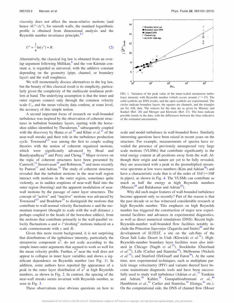
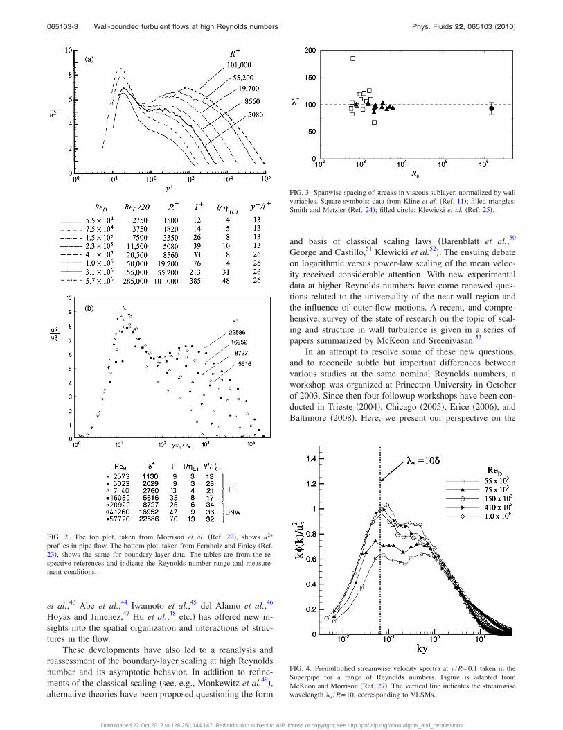
Given this more recent background, it is not surprisingthat distributions of the turbulence intensity, particularly thestreamwise component u2, do not scale according to thesimple inner-outer arguments that seemed to work so well forthe mean velocity profile. Further, u2 near the wall does notappear to collapse in inner layer variables and shows a sig-nificant dependence on Reynolds number �see Fig. 1�. Inaddition, some authors have reported the appearance of apeak in the outer layer distribution of u2 at high Reynoldsnumbers, as shown in Fig. 2. In contrast, the spacing of thenear-wall streaks seems invariant with Reynolds number, asseen in Fig. 3.

These observations raise obvious questions on how to

scale and model turbulence in wall-bounded flows. Similarlyinteresting questions have been raised in recent years on thestructure. For example, measurements of spectra have re-vealed the presence of previously unsuspected very largescale motions �VLSMs� that contribute significantly to thetotal energy content at all positions away from the wall. Al-though their origin and nature are yet to be fully revealed,they are associated with a peak in the premultiplied stream-wise spectrum at low wave numbers �Kim and Adrian26� andhave a characteristic scale that is of the order of 10� ��10Rin pipes�, as shown in Fig. 4. The VLSMs can contribute asmuch as half the energy at high Reynolds numbers�Marusic28 and Balakumar and Adrian29�.

Why did such major features of wall-bounded turbulencebecome apparent only so recently? Part of the reason is thatthe past decade or so has witnessed considerable research athigh Reynolds number. This emphasis on high Reynoldsnumber has triggered the construction of major new experi-mental facilities and advances in experimental diagnostics,as well as direct numerical simulations �DNS�. Recent high-Reynolds-number wall-bounded flow facilities notably in-clude the Princeton Superpipe �Zagarola and Smits�30 and thedevelopment of SLTEST, a site on the salt-flats of theGreat Salt Lake Desert in Utah �Klewicki et al.31�. High-Reynolds-number boundary layer facilities were also initi-ated in Chicago �Nagib et al.32�, Stockholm �Österlundet al.33�, Lille �Carlier and Stanislas34�, Melbourne �Nickelset al.35�, and Stanford �DeGraaff and Eaton36�. At the sametime, new experimental techniques, such as multiplane par-ticle image velocimetry �PIV� and variants thereof have be-come mainstream diagnostic tools and have been success-fully used to study wall turbulence �Adrian et al.,37 Tomkinsand Adrian,38 Kahler,39 Ganapathisubramani et al.,40

Hambleton et al.,41 Carlier and Stanislas,34 Elsinga,42 etc.�.On the computational side, the DNS of channel flow �Moser

FIG. 1. Variation of the peak value of the inner-scaled streamwise turbu-lence intensity with Reynolds number �which occurs around y+�15�. Thesolid symbols are DNS results, and the open symbols are experimental. Thecircles indicate boundary layers, the squares are channels, and the trianglesare for ASL data. The sources for the data are as given by Marusic andKunkel �Ref. 20� and Metzger and Klewicki �Ref. 21�. The lines indicatepossible trends in the data, with the differences between the lines indicativeof the estimated uncertainties.

065103-2 Marusic et al. Phys. Fluids 22, 065103 �2010�


et al.,43 Abe et al.,44 Iwamoto et al.,45 del Alamo et al.,46

Hoyas and Jimenez,47 Hu et al.,48 etc.� has offered new in-sights into the spatial organization and interactions of struc-tures in the flow.

These developments have also led to a reanalysis andreassessment of the boundary-layer scaling at high Reynoldsnumber and its asymptotic behavior. In addition to refine-ments of the classical scaling �see, e.g., Monkewitz et al.49�,alternative theories have been proposed questioning the form

and basis of classical scaling laws �Barenblatt et al.,50

George and Castillo,51 Klewicki et al.52�. The ensuing debateon logarithmic versus power-law scaling of the mean veloc-ity received considerable attention. With new experimentaldata at higher Reynolds numbers have come renewed ques-tions related to the universality of the near-wall region andthe influence of outer-flow motions. A recent, and compre-hensive, survey of the state of research on the topic of scal-ing and structure in wall turbulence is given in a series ofpapers summarized by McKeon and Sreenivasan.53

In an attempt to resolve some of these new questions,and to reconcile subtle but important differences betweenvarious studies at the same nominal Reynolds numbers, aworkshop was organized at Princeton University in Octoberof 2003. Since then four followup workshops have been con-ducted in Trieste �2004�, Chicago �2005�, Erice �2006�, andBaltimore �2008�. Here, we present our perspective on the

FIG. 2. The top plot, taken from Morrison et al. �Ref. 22�, shows u2+

profiles in pipe flow. The bottom plot, taken from Fernholz and Finley �Ref.23�, shows the same for boundary layer data. The tables are from the re-spective references and indicate the Reynolds number range and measure-ment conditions.

FIG. 3. Spanwise spacing of streaks in viscous sublayer, normalized by wallvariables. Square symbols: data from Kline et al. �Ref. 11�; filled triangles:Smith and Metzler �Ref. 24�; filled circle: Klewicki et al. �Ref. 25�.

FIG. 4. Premultiplied streamwise velocity spectra at y /R=0.1 taken in theSuperpipe for a range of Reynolds numbers. Figure is adapted fromMcKeon and Morrison �Ref. 27�. The vertical line indicates the streamwisewavelength �x /R=10, corresponding to VLSMs.

065103-3 Wall-bounded turbulent flows at high Reynolds numbers Phys. Fluids 22, 065103 �2010�


new insights gained from these workshops. We aim to syn-thesize the main points and highlight the issues that need tobe resolved, without presenting a comprehensive review ofall the topics. We also consider other recent advances andpoint out where important differences of opinion persist, soas to mark the beginning of their resolution.

II. HIGH-REYNOLDS-NUMBER EXPERIMENTS

The Reynolds number dependence of turbulence quanti-ties, whenever observed, is generally weak, scaling withsomething like the log of the Reynolds number. Therefore, itis essential to have access to high-Reynolds-number flows or,even more invaluably, facilities that can achieve a largerange of Reynolds numbers. Table I summarizes the principalsources of data with Re�4000 that have been consideredduring the workshops, where Re� is the friction Reynoldsnumber, also called the Kármán number, defined as the ratioof the boundary layer thickness � or pipe radius or channelhalf-height to the friction length scale � /U�. Many of thesesites have only come online in the past decade and, in addi-tion, large facilities are at various stages of planning now.These include the CICLoPE pipe described by Talamelliet al.59 and the New Hampshire wind tunnel.60

In addition to the access to the necessary facilities, ac-curate measurements are required to identify the often subtlescaling trends in wall-bounded flows. This may seem like anelementary statement to make, but since the largest scale ofthe flow ��, R, or h� is fixed by the size of the facility, theviscous scale becomes small at high Reynolds number, and amajor challenge to the experimentalist is to maintain a suffi-ciently small measurement volume to avoid spatially averag-ing the smallest scales. Accurate measurements also requireparticular attention to the details of calibration and the re-sponse of the instrumentation. Both of these issues will beconsidered in more detail when discussing the available ex-perimental data. We first consider some specific aspects ofthe experimental facilities themselves.

A. Atmospheric surface layer data

The near-neutral atmospheric surface layer �ASL� hasbeen a historic source of very high Reynolds numbers, andthe establishment of the Surface Layer Turbulence and En-vironmental Science Test �SLTEST� site on the salt playa ofUtah’s Western desert by Metzger and Klewicki21 andMetzger61 has been very influential. The strategic importanceof the near-neutral ASL is clear: it represents some of the

TABLE I. Compilation of experiments considered extensively in the Workshops. OFI indicates oil-film inter-ferometry, HW hot wires, P pressure drop, � is the von Kármán constant, and U� is the friction velocity.

ReferenceFlowtype

HighestRe� �

y+: startof log law

No. of decadesof log law

U�

methodU

meas. tech.

McKeon et al.a Pipe 300 000 0.421 600 1.8 P Pitot/HW

Morrison et al.b

Princeton Superpipe

Montyc Pipe 4000 0.384 100 0.8 P Pitot/HW

Melbourne

Montyc Channel 4000 0.389 100 0.8 P Pitot/HW

Melbourne

Zanoun et al.d Channel 4800 0.37 150 0.8 P HW

Erlangen

Nagib et al.e BL 22 000 0.384 200 1.4 OFI HW

NDF, Chicago

Österlund et al.f BL 14 000 0.38 200 1.0 OFI HW

KTH, Stockholm

Nickels et al.g �2007� BL 23 000 0.39 200 1.5 OFI Pitot/HW

ICET �Duncan et al.h�Melbourne

Metzger & Klewicki BL O�106� ¯ ¯ �3 ¯ HW

SLTEST, Utah

aReference 54.bReference 22.

cReference 55.dReference 56.

eReference 32.fReference 33.

gReference 57.hReference 58.



highest Reynolds number conditions that can be achievedterrestrially �and without the stringent constraints on proberesolution imposed by smaller-scale boundary layers�. Thereis evidence that the ASL near-wall turbulence �Metzger andKlewicki,21 Marusic and Hutchins,62 etc.� and pressure field�Klewicki et al.63� scale in a manner similar to the canonicalturbulent boundary layer. At the least, the ASL anchors Rey-nolds number trends in ways that would not be possibleotherwise.

It should be noted, however, that the experimental chal-lenges of obtaining high quality ASL data are severe, andconsiderable effort has been spent assessing the suitability ofthe ASL as a model for the canonical boundary layer. Ofmajor importance is the issue of statistical convergence aris-ing from the nonstationarity of the ASL, specifically due to alimited period of near neutrality, wind speed, and direction.Other questions are the importance of thermal effects asso-ciated with the passage through near neutrality, fetchconditions �that is, topological and surface roughness varia-tions�, the upstream and “free stream” boundary conditions,and so on.

B. Wall shear stress data

For boundary layer flows, a major limitation is that thereis still no sufficiently accurate way to measure the wall shearstress �and hence U�� for all surface conditions. One ideallyneeds an accuracy of perhaps �0.5% or better �see Nagibet al.32� to draw definitive conclusions. Clearly, a Clauserchart approach cannot be used to test the validity of the loglaw as it assumes it a priori. Oil-film interferometry is per-haps the best direct measurement method but its accuracy isstill limited to no better than �1% to 2% �e.g., Ruedi et al.,64

Fernholz et al.,65 and Monkewitz et al.49�. It is also limited togas flows and nonrough surface conditions. For pipes andchannels, the situation is more straightforward as the wall-shear stress is known for fully developed flows from thepressure drop along the length of the pipe or channel. How-ever, channel facilities must have aspect ratios much largerthan 10 to minimize side wall effects on the wall shear stressand on the flow field, in general. The experiments listed inTable I use an independent measure of wall-shear stress. Thetable shows the reported value of the von Kármán constant �,the length of the documented log region, and where the loglaw is reported to begin. These issues will be discussed laterin Sec. III B. Note that for historical reasons we refer to � asa constant while it may indeed be a variable coefficient asdiscussed later.

C. Evolution from initial conditions

An important issue with respect to the experimental fa-cilities is the evolution from initial conditions: the develop-ment length in pipes and channels and the effects of up-stream history on the development of boundary layers. Thefact that in many experiments these effects are not, or onlyincompletely, documented is one of the principal causes ofpast and present disagreements between different experi-ments and their interpretations.

1. Pipe and channel flows

An issue raised in connection with the design of theCICLoPE pipe by Talamelli et al.59 was the minimum devel-opment length for a pipe or channel flow to be regarded asfully developed. The definition of fully developed requiresthat all mean flow quantities �that is, velocity field and pres-sure gradient� and all turbulence quantities �i.e., u2, spectra,skewness, flatness, etc.� should become independent ofstreamwise location. A survey of the existing literature onpipe flows reveals considerable variation in what is consid-ered a sufficient development length, where many workershave chosen to go longer as a precaution �which is perhaps awise decision if the option is available�. For example, whileNikuradse66 used 40D, where D is the pipe diameter, Perryet al.67 used 398D, and Zagarola and Smits30 used 164Dbased on an assessment of the Reynolds number dependenceof the transition length, the development of the turbulentwall boundary layers and a large-eddy development length.

In response to this practical query, Doherty et al.68 con-ducted a series of detailed experiments in the Melbournepipe, the same facility originally used by Perry et al.67 Hot-wire velocity profile measurements were made at streamwiseintervals of 2.5D starting from the pipe entrance to a lengthof 228D for bulk Reynolds numbers of 105 and 2.0�105.They concluded that the mean velocity invariance wasachieved at approximately 50D, while higher order statistics�up to flatness� required 80D of development length. It ispossible that longer development lengths will be required athigher Reynolds numbers, but the Melbourne experimentsprovide important guidance for large projects such asCICLoPE where the large pipe diameter �D�0.9 m� wouldentail substantial costs for any extra length of pipe.

Similar experiments were also carried out by Monty55

and Lien et al.69 in the Melbourne channel flow facility toinvestigate the required development length for turbulentchannel flow. Here only mean velocity profiles were mea-sured and it was concluded that 130 channel heights of de-velopment distance were required for invariance of the meanvelocity field for bulk Reynolds numbers ranging from4.0�104 to 1.85�105. We do not fully understand the dif-ference from the pipes. The challenge of a longer develop-ment length in channel flows, exacerbated by the require-ments on the aspect ratio and the larger flow rate required toreach the same Reynolds number as in a pipe, makes theconstruction of truly high-Reynolds-number channel facili-ties exceedingly difficult; see Zanoun et al.70 This is unfor-tunate in view of the emphasis given to this flow field inDNS of wall-bounded turbulence. As an outcome of thiswork, the DNS of pipe flows is being encouraged, and a fewdata sets are now becoming available �for example, Wu andMoin71�.

2. Boundary layers

For ZPG boundary layers, issues related to streamwiseevolution are considerably more complex. Discussions at theworkshops, and a survey of existing literature, revealed thatsome confusion and disagreement still exists concerning theuse of the term equilibrium, or what constitutes a well-



behaved flow. A strict definition of equilibrium according toTownsend4 and Rotta7 requires all mean-relative motions andenergy-containing components of turbulence �for example,Reynolds shear stress and the turbulence intensities� to havedistributions that become invariant with streamwise develop-ment when scaled with local length and velocity scales �see,especially, Narasimha and Prabhu72�. Rotta7 demonstratedthat the only wall-bounded flow for which this can occur ona hydrodynamically smooth surface is the sink flow, and thiscondition was experimentally validated by Jones et al.73

In boundary layers other than the sink flow, not even themean velocity can be described from the wall to the freestream by a function of a single similarity variable. At leasttwo similarity variables, y+=yU� /� and y /� are required.Therefore, the above strict definition of equilibrium needs tobe relaxed: In the boundary layer one might speak of equi-librium when the mean velocity deficit U�−U in the outerpart exhibits self-similarity, since this region dominates atlarge Reynolds numbers.

The commonly held view is that the mean-velocity pro-file in all ZPG boundary layers would be self-similar accord-ing to the above definition when the Reynolds number issufficiently high. This stems largely from the interpretationof data correlations with Reynolds number, such as the oneby Coles74 for the wake factor �, which becomes nominallyconstant for Re �8000, Re being the Reynolds numberbased on momentum thickness. Significant scatter in the datahas led to questions about the validity of the experimentsused in the correlation. It has also motivated new theories byCastillo and Johansson75 and others to introduce additionalparameters to explain the deviation of some data sets fromclassical scaling. Another possible explanation for the scatteris the rather strong dependence of � on the method by whichit is extracted from the data and, more generally, on howsensitive � and � are to the particular fit used for the outerpart of the mean velocity profile �see Monkewitz et al.,76 fora detailed discussion�.

It is also important to keep in mind that each experimen-tal �and computed� boundary layer must develop from aunique set of upstream boundary conditions. Here we arereferring to inflow conditions and tripping/transition devices,and not to poorly designed experiments affected by highfree-stream turbulence, three dimensionality, or spuriouspressure gradients. For example, a boundary layer develop-ing on a short plate at high speed may have the same Re asa boundary layer developing on a long plate at low speed,but not necessarily the same value of the shape factorH=�� / and/or of �, unless the development length of bothlayers has been sufficient; see the recent discussions byChauhan and Nagib77 and Castillo and Walker.78 What is thesufficient development length for a ZPG boundary layer tobecome independent of initial conditions? In general, thisquestion is still open, but the answer must depend on thespecific initial conditions, on the quantity being considered,and on the desired degree of independence, which needs tobe quantified. In other words, a flow is not fully character-ized by its Reynolds number alone.

Recent progress on the easier problem of quantifying thedeviation from the canonical equilibrium state has been en-

couraging, largely because many of the new experiments ob-tained the wall stress by independent means, and have care-fully documented the evolution of the boundary layer withdownstream distance. However, additional data from differ-ent facilities are required before many of the questions canbe answered satisfactorily, and this has become a focusfor ongoing collaborative efforts. Significant advanceshave been made by Nagib et al.,32 Chauhan et al.,79 andMonkewitz et al.,49 who have proposed criteria to quantifywhen ZPG boundary layers are well behaved. Their criteriaare based on the assumption that the canonical asymptoticstate is attained when � reaches a constant value and/or thevalues of skin friction and shape factor are consistent witheach other in the framework of classical theory. They arguethat, once the asymptotic state is reached, the influence ofinitial conditions should appear only in a virtual origin,which is a correction of the nominal streamwise position xalong the plate. Figure 5 shows how a large collection ofexisting data compares, with and without the virtual origincorrection. The uncorrected data illustrate the high degree ofvariability among different experiments, as discussed above.The globally successful correction is based on the asymptoticboundary layer growth �� /x��2 / ln2�Rex� derived byMonkewitz et al.49 from the log law without arbitrary datafitting.

The more difficult problem of how the canonicalasymptotic state evolves from an arbitrary initial conditionwas first tackled by Perry et al.80,81 who computed the devel-opment of the ZPG boundary layer from a specified set ofinitial conditions using the momentum and continuity equa-tions in simplified form. This involves the hypotheses thatthe total shear stress field is uniquely described by a two-

FIG. 5. Variation of normalized boundary layer development without �x /��,top part, and with correction �x /�� for virtual origin �bottom�. Taken fromChauhan et al. �Ref. 79�. Here a total of 471 data points are shown, wherethe different symbols represents results that satisfy different levels of criteriaaccording to Chauhan et al. �Ref. 79�. “�” indicate where the criteria fail.The solid line is the theoretical result from Monkewitz et al. �Ref. 49� inconjunction with numerical integration of a composite profile fit to the meanvelocity profile.



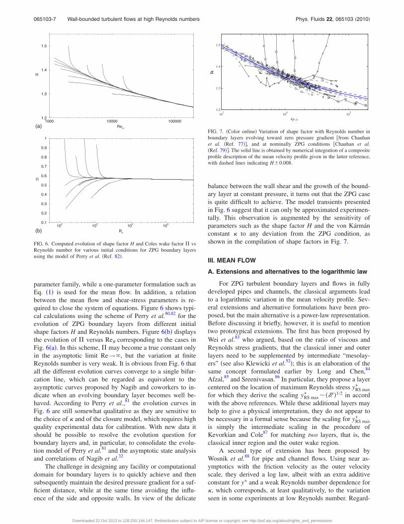
parameter family, while a one-parameter formulation such asEq. �1� is used for the mean flow. In addition, a relationbetween the mean flow and shear-stress parameters is re-quired to close the system of equations. Figure 6 shows typi-cal calculations using the scheme of Perry et al.80,82 for theevolution of ZPG boundary layers from different initialshape factors H and Reynolds numbers. Figure 6�b� displaysthe evolution of � versus Re corresponding to the cases inFig. 6�a�. In this scheme, � may become a true constant onlyin the asymptotic limit Re→�, but the variation at finiteReynolds number is very weak. It is obvious from Fig. 6 thatall the different evolution curves converge to a single bifur-cation line, which can be regarded as equivalent to theasymptotic curves proposed by Nagib and coworkers to in-dicate when an evolving boundary layer becomes well be-haved. According to Perry et al.,81 the evolution curves inFig. 6 are still somewhat qualitative as they are sensitive tothe choice of � and of the closure model, which requires highquality experimental data for calibration. With new data itshould be possible to resolve the evolution question forboundary layers and, in particular, to consolidate the evolu-tion model of Perry et al.81 and the asymptotic state analysisand correlations of Nagib et al.32

The challenge in designing any facility or computationaldomain for boundary layers is to quickly achieve and thensubsequently maintain the desired pressure gradient for a suf-ficient distance, while at the same time avoiding the influ-ence of the side and opposite walls. In view of the delicate

balance between the wall shear and the growth of the bound-ary layer at constant pressure, it turns out that the ZPG caseis quite difficult to achieve. The model transients presentedin Fig. 6 suggest that it can only be approximated experimen-tally. This observation is augmented by the sensitivity ofparameters such as the shape factor H and the von Kármánconstant � to any deviation from the ZPG condition, asshown in the compilation of shape factors in Fig. 7.

III. MEAN FLOW

A. Extensions and alternatives to the logarithmic law

For ZPG turbulent boundary layers and flows in fullydeveloped pipes and channels, the classical arguments leadto a logarithmic variation in the mean velocity profile. Sev-eral extensions and alternative formulations have been pro-posed, but the main alternative is a power-law representation.Before discussing it briefly, however, it is useful to mentiontwo prototypical extensions. The first has been proposed byWei et al.83 who argued, based on the ratio of viscous andReynolds stress gradients, that the classical inner and outerlayers need to be supplemented by intermediate “mesolay-ers” �see also Klewicki et al.52�; this is an elaboration of thesame concept formulated earlier by Long and Chen,84

Afzal,85 and Sreenivasan.86 In particular, they propose a layercentered on the location of maximum Reynolds stress yRS max

+

for which they derive the scaling yRS max+ ��+�1/2 in accord

with the above references. While these additional layers mayhelp to give a physical interpretation, they do not appear tobe necessary in a formal sense because the scaling for yRS max

+

is simply the intermediate scaling in the procedure ofKevorkian and Cole87 for matching two layers, that is, theclassical inner region and the outer wake region.

A second type of extension has been proposed byWosnik et al.88 for pipe and channel flows. Using near as-ymptotics with the friction velocity as the outer velocityscale, they derived a log law, albeit with an extra additiveconstant for y+ and a weak Reynolds number dependence for�, which corresponds, at least qualitatively, to the variationseen in some experiments at low Reynolds number. Regard-

1000 10000 100000Re��

1.2

1.3

1.4

1.5

H

(a)

103 104 105 106R�

0.1

0.2

0.3

0.4

0.5

0.6

0.7

0.8

0.9

1

�

(b)

FIG. 6. Computed evolution of shape factor H and Coles wake factor � vsReynolds number for various initial conditions for ZPG boundary layersusing the model of Perry et al. �Ref. 82�.

103 104 1051.2

1.3

1.4

1.5

� � � �

FIG. 7. �Color online� Variation of shape factor with Reynolds number inboundary layers evolving toward zero pressure gradient �from Chauhanet al. �Ref. 77��, and at nominally ZPG conditions �Chauhan et al.�Ref. 79��. The solid line is obtained by numerical integration of a compositeprofile description of the mean velocity profile given in the latter reference,with dashed lines indicating H�0.008.



ing the additive constant in the logarithmic profile, B, it mustbe considered as a higher order correction integrated into theleading order logarithmic profile. Since the logarithmic partof the velocity profile is centered on y+ of order Re��

1/2�1

�see above�, ln�y++a+� can be expanded as ln�y+�+ �a+ /y+�+O�1 /y+�2. In other words, while such a shift of origin mayimprove the fit at low Reynolds numbers, it most likely rep-resents only part of the complete higher order correction.Other studies have also noted the possibility of a log lawwith a shifted origin, including Oberlack,89 Lindgren et al.,90

and Spalart et al.91

Returning to the power-law alternatives, Barenblatt92

showed that if Reynolds number effects persist at all Rey-nolds numbers the similarity is incomplete and, as a conse-quence, the mean velocity follows power laws withReynolds-number-dependent exponents for pipes and chan-nels, and �with further attributes� also in boundary layers. Healso remarked on physical mechanisms that could bringabout this persistent dependence on viscosity even in theouter layer. These studies have been discussed at somelength, and we will not directly add much to that discussion.George and Castillo51 and George93,94 argued that the scalingbehavior in boundary layers is different from that in pipesand channels since the boundary layer is not homogeneous inthe streamwise direction with the consequence, among oth-ers, that there is no justification for using the friction velocityas the velocity scale for both the inner and outer regions. Indeveloping an alternative scaling, George and Castillo51 sug-gested the asymptotic invariance principle that requires aconsistent scaling of the equations at all Reynolds numbers.Therefore, based on the asymptotic behavior of the meanmomentum equation and requiring a similarity solution forRe�=�+→�, they conclude that U�, the freestream velocity,is the only theoretically acceptable velocity scale for theouter region. This leads to a power-law representation for themean flow. Recently Jones et al.95 have challenged the asser-tion that U� is the only acceptable velocity scale using the-oretical arguments and show that U� is equally acceptable inthe asymptotic limit. Also, arguing along the lines ofPanton,96 the outer expansion of the mean velocity Uouter

�U�+O�U�� should be made nondimensional with U� toyield U /U�=1+O�1 /U�

+�. While this is so far equivalent tothe classical formulation, it may be helpful for future theo-retical developments.

The debate over power law versus log law may continueuntil very clear differences can be shown in high-fidelityexperimental data at high Reynolds numbers. The real diffi-culty is that experiments are unlikely to ever revealasymptotic conditions for a boundary layer. Indeed, one canevaluate the viability of an asymptotic theory only in thecontext of finite-Reynolds-number corrections, which notheory has satisfactorily produced thus far. For example, theasymptotic limit corresponds to U�

+ →�, while for the ASLtypical values are U�

+ =40 �and for a boundary layer that ismarginally past transition U�

+ �18�. Hence, for incompress-ible flows U�

+ →� quickly requires a boundary layer of in-tergalactic reach, and the limit is practically irrelevant. Nev-ertheless, a mathematically sound description of the

turbulent boundary layer should be well behaved in theasymptotic limit. Recent efforts by Monkewitz et al.49 tacklethis problem by considering the self-consistency of leadingorder terms in asymptotic expansions and finding clear sup-port for the classical scaling and the log law. Monkewitzet al.76 also compared a multitude of high-Reynolds-numberexperimental data to the classical scaling and the two mainpower-law theories and conclude that the log law is empiri-cally superior.

B. Asymptotic regime

The issue considered here is the minimum separation ofscales required in practice for the mean flow to reach a ca-nonical asymptotic state. It is clear that there is strictly nothreshold value, but that the problem needs to be posed asfollows: for the asymptotic state to be approached within apreset allowable accuracy, the scale ratio has to be above acertain number. Within the classical framework, this questionhas become almost synonymous with determining the mini-mum Reynolds number required to observe a clear logarith-mic variation in the profile, which in turn is closely related tothe question of the extent of the logarithmic layer. Given Eq.�1�, the log law should begin at a fixed value of y+, while theexperiments in Table I give estimates between 100 and 600.In ZPG boundary layers, the extent of a clear log law esti-mated by Nagib et al.32 from recent experimental data isy+�200 and y /��0.12. Recent analyses have suggested thatthe start of the log law may depend on Reynolds number orflow conditions, as discussed below. Wosnik et al.88 con-cluded that a mesolayer exists in the range 30�y+�300where there cannot be sufficient scale separation to reachhigh-Reynolds-number characteristics. Lindgren et al.,90 fol-lowing the Lie group analysis of Oberlack,89 proposed thatno log law exists for y+�200 owing to an offset in y.

A rather different estimate has been extracted byZagarola and Smits30 and McKeon et al.54 from the veryhigh-Reynolds-number experiments in the Princeton Super-pipe. They suggested that a self-similar log region was ob-served only for y+600 and y /R�0.12 �with a power-lawregion for y+�600�, corresponding to a minimum Reynoldsnumber Re��5000. This Reynolds number signaled a suffi-cient scale separation for a consistent scaling of the pipefriction factor, collapse of the streamwise fluctuations inouter scaling, and the attainment of a constant ratio of theso-called Zagarola and Smits outer velocity scale to the fric-

tion velocity, �= �UCL− U� /u� �see Fig. 8�. However, itshould be noted that the distinct transitions in behavior ob-served in the Superpipe have not been replicated in otherflows �which, however, do not span the same Reynolds num-ber range�. Thus, some questions as to the nature of thesechanges still remain unanswered, and for this the plannedCICLoPE experiments will be very valuable.

An alternative place to search for log laws is in the DNSdata. Recent advances have seen channel simulations exceedRe�=2000 �Hoyas and Jimenez47� for large box domains�8�� in the streamwise direction�. Jimenez and Moser98 con-sidered the mean velocity scaling for a range of Reynoldsnumbers and concluded that no clear log law exists at these



Reynolds numbers. However, by comparing their data to thelog law including finite Reynolds number corrections basedon a matched asymptotic analysis �such as those described inAfzal99 and Panton96�, they concluded that an overlap regionmay exist for y /��0.45 and y+�300. This discussion em-phasizes that a lower boundary y+ for the log law �or itsalternatives� is to be regarded only in an asymptotic contextas a large number whose numerical value depends amongother things on the desired accuracy.

These numerical simulations and recent experimentshave shown that it is essential to have sufficiently highReynolds number before one can actually see a log region orany other asymptotic behavior of boundary layer parameters.It is still not entirely clear how high it must be, or whetherthe answers depend on development length or evolution his-tory. Based on a survey of the available data for differentflows, a reasonable estimate seems to be a nominal Re� inexcess of 4000–5000, although to see a decade of logarith-mic variation may require Re� in excess of 40 000–50 000.

There remains the issue of how to compare turbulentboundary layers with pipe and channel flows. Most oftencomparisons are made on the basis of Re�=�+=R+, where Ris the pipe radius or the channel half-height. However, in theboundary layer the flow is essentially nonturbulent fory��, while it is turbulent for y�R in the pipe and channel.Therefore, one would expect that the centerline of a pipe orchannel y+=R+ corresponds to a location y+��+ well withinthe flat-plate boundary layer. To make progress, one mayconsider the location of the maximum Reynolds shear stressin pipes and channels, yRS max

+ �2�Re��1/2 �Sreenivasan86 andSreenivasan and Sahay100� to the one in ZPG boundary lay-ers, yRS max

+ �2�Re��1/2 �Monkewitz and Nagib101�. This sug-gests that R+�Re� in pipes and channels should possibly becompared to Re�� and not �+ in ZPG boundary layers. This isequivalent to saying that the physically appropriate outerscale in the boundary layer is the Rotta–Clauser scale=��U�

+ and not the nominal boundary layer thickness �,even though the two are asymptotically proportional in theframework of the classical theory � /��3.5 according toChauhan et al.102�. Hence, the “closeness” to asymptotic con-ditions in boundary layers and pipes and channels is charac-terized by Re�� and Re�, respectively. Some support comes

from the estimates of Reynolds number for the mean velocityprofile to reach its final self-similar shape: while Monkewitzet al.49 have suggested Re��104 �corresponding to�+�2500� for the ZPG boundary layer, Nagib andChauhan103 proposed Re��8000 for channels and pipes.However, it is unclear at this point whether comparisons ofboundary layers with pipes and channels are limited in prin-ciple.

As has become clear from the above discussions, to re-solve questions regarding the extent of the logarithmic layer,it is useful to examine the problem in the framework ofmatched asymptotic expansions �MAEs�, although it is con-ceded that one needs to assume beforehand the inner andouter scales, and that a choice needs to be made of the gaugefunctions for the series expansion. The most recent studies ofasymptotic expansions are by Panton,96,104 who examined themean flow and the Reynolds stresses in wall turbulence. Withsome assumptions, this analysis gives insights into the innerand outer region interactions. In a MAE approach to themean flow, the logarithmic profile is the leading order com-mon part of inner and outer expansions. Therefore, at anyfinite scale separation or Reynolds number, this leading ordercommon part will always be contaminated from both sides:from the wall by higher order terms of the asymptotic expan-sion of the inner mean velocity fit and from the free streamby higher order terms of the expansion of the outer fit. Thismeans that the question of the boundaries of the logarithmicregion is ill posed as long as one does not specify whatdeviation from the exact log law one wants to tolerate. In thissense, if one accepts that the log law is the asymptotic ve-locity profile in the overlap region, one might state some-what tautologically that the log law is always present even ifit is completely overwhelmed by the inner and outer expan-sions. The DNS of Jimenez and Moser98 appears to be a casein point.

1. Universality of �?

The variation of the � values shown in Table I highlightsanother unsettled issue that is closely related to the abovediscussion. Without the results of the Superpipe experimentsat the higher Reynolds numbers, and those from wall-bounded flows under a wide range of pressure gradients assummarized by Nagib and Chauhan,102,103 one may concludethat � is constant within the uncertainty of measuring wall-shear stress. Such a view is supported by the pipe and chan-nel flow results of Monty,55 which yielded a von Kármánconstant that is identical �within error bars� to the ones ex-tracted from the KTH and NDF ZPG boundary layers �seeTable I�. Figure 9 shows the hot-wire mean-velocity profilesfrom Monty55 on which this conclusion is based. However,we have the view that � is indeed not a universal constantand is measurably different for different flows.

The view that the von Kármán constant may not be uni-versal emerged from the studies of flat-plate boundary layerswith pressure gradient by Nagib et al.106 and Chauhanet al.102 and has been supported by the recent work ofDixit and Ramesh107 and Bourassa and Thomas.108 Nagibet al.102,106 advocated that � is a function of pressure gradi-

FIG. 8. Variation of the ratio of the Zagarola and Smits outer velocity scale

to the friction velocity, �= �UCL− U� /u�, with Reynolds number in pipe flow,from McKeon �Ref. 97�.



ent, noting that this conclusion requires an independentmethod of determining U�. The evidence for this was re-vealed when equilibrium boundary layers under various pres-sure gradients were investigated with oil film interferometryand hot-wire measurements at high Reynolds numbers. Fig-ure 10 reproduces some of their results and depicts the varia-tion of skin friction as a function of momentum-thicknessReynolds number for adverse and favorable pressure gradi-ents �FPGs�, contrasted with the ZPG case we have focusedon here. The trends of the curves in Fig. 10 demonstrate thatthe von Kármán constant must be different between the threecases with its value largest for the FPG case. Nagib andChauhan103 also suggested that � is different for ZPG bound-ary layers, pipes and channels. This is based on estimates of� using composite profiles, and a compilation of data fromNagib and Chauhan103 is shown in Fig. 11. Since the sameasymptotic composite profile without low-Reynolds-numbercorrections is fitted at all Reynolds numbers, a variation ofthe fitted � emerges, as seen on the figure. The idea is that at

large enough Reynolds number this fitted � reaches aconstant “asymptotic” � which is then identified with the“true” �.

The Melbourne pipe and channel experiments55 involvedmeasurements with hot wires and total-head probes, whichwere in good agreement after the total-head probe resultswere corrected for shear effects using the MacMillan109 cor-rection and for turbulence effects. However, the � valuesfrom the Melbourne pipe and channel are at odds with thevalues of 0.421 obtained in the Superpipe by McKeon et al.54

and 0.37 in the channel obtained by Zanoun et al.56 In thecase of channels, the differences may be due to the role ofthe aspect ratio of the experimental facilities in the develop-ment of the flow and other aspects of determining �. For thepipe flows, it remains uncertain whether the Reynolds num-bers of the Melbourne facility are still too low to exhibitasymptotic behavior. Recall that the Superpipe results sug-gest a lower end of the log law at y+=600, which corre-sponds to the outer end of the log layer reported by Monty.55

The exact asymptotic value of � extracted by the approach ofNagib and Chauhan103 for different flows also plays an im-portant role in this discussion of the Superpipe data. As dem-onstrated in Fig. 11, Monty’s results �filled circles� are con-sistent with �’s extracted from other experiments and DNS;see e.g., the Superpipe values at lower Reynolds numbers. Inthis regard, one puzzling observation is the trend of the fitted� with Reynolds number: most of the data appear to ap-proach the asymptotic value from above for boundary layersand channels and from below for pipes.

Further work is needed to explain the above trends anddifferences, and new collaborative measurement initiativesare underway to address these issues. Since the Superpipe isunique and has produced results at Reynolds numbers farexceeding any previous studies, they have become perhapsthe most scrutinized set of experimental data since those ofNikuradse in the 1930s. However, probe corrections pose achallenge. At the higher Superpipe Reynolds numbers thesmallest physically practical total head probe has a diameterof several hundred viscous units, which is well outside therange in which the probe corrections have been empiricallydetermined. Also, effects of surface roughness may comeinto play at Reynolds numbers exceeding 24�106. McKeonet al.110 and McKeon and Smits111 have proposed new, high-

FIG. 9. Pipe and channel flow hot-wire mean velocity profiles of Monty�Ref. 55�. Top profiles show pipe flow results: “�” Re=40 000; “�”Re=54 000; “�” Re=69 000; “�” Re=89 000; “�” Re=133 000. Bottomprofiles show channel flow results: “�” Re=40 000; “�” Re=60 000; “�”Re=73 000; “�” Re=108 000; “�” Re=141 000; “�” Re=182 000. Dot-ted lines are the DNS data of Spalart �Ref. 105� for the near-wall regiononly.

0.0014

0.0018

0.0022

0.0026

0.0030

0.0034

0 10,000 20,000 30,000 40,000 50,000 60,000Re �

Cf

ZPG

FPG

APG

FIG. 10. �Color� Variation of skin friction with pressure gradient for equi-librium boundary layers under favorable �FPG�, zero �ZPG�, and adverse�APG� pressure gradients; from data of Chauhan and Nagib �Ref. 102�.

FIG. 11. Nagib and Chauhan �Ref. 103� estimated variation of the � for inpipes, channels, and ZPG boundary layers obtained using composite pro-files. The symbols are as given in by Nagib and Chauhan �Ref. 103� formultiple datasets, including their evaluation of Monty’s results �shown with“�” for pipe and channel�, together with Superpipe data: “�,” Superpipe,static+probe corrected; “�,” Superpipe, static corrected; “�,” Superpipe,uncorrected. “——,” �P=0.41; “–·–·–,” �C=0.37; “- - -,” �BL=0.384.



Reynolds-number corrections for both total head probes andthe wall pressure tappings that supersede previous methodsof measuring the static pressure when probe size becomes aconcern. The resolution of the issue of probe corrections isbeing actively pursued by a multinational measurement col-laboration, which includes a comparison between measuringdevices with different measuring volumes. Furthermore, anindependent confirmation of the Superpipe results is plannedin the CICLoPE facility under construction in Italy, whichinvolves fully developed flow in a 0.9 m diameter pipe. Thebulk Reynolds number will be nominally limited to 2�106,considerably smaller than the 30�106 achieved in the Su-perpipe. Even so, in the CICLoPE pipe the probe size effectswill be reduced because of the larger pipe diameter and thereis expected to be sufficient overlap with the Superpipe datato allow for rigorous comparisons.

Definitively resolving the issue of whether � is a univer-sal constant or not requires higher accuracy measurementsfor both the mean flow and the wall shear stress, coupledwith theory-based consistency checks between these two in-dependent measurements. At this point we are leaning to-ward a flow-dependent � and note that while some may notconsider such detailed arguments about � very significant,they are crucial to modeling and to numerical simulations ofwall-bounded flows. Fundamentally, if � is indeed variableand depends on the flow and the Reynolds number, it ishardly consistent with a universal logarithmic law.

C. Beyond the mean flow

To close this section, we reiterate that the required accu-racy for skin friction and velocity measurements is unrealis-tically high to fully resolve all the above questions about theform of the mean velocity profile. While further high-Reynolds-number experiments are clearly needed, we con-sider it more promising to move toward theories that incor-porate fluctuation statistics rather than dealing merely withthe mean velocity, which may well be the least sensitive toReynolds number variation. Some efforts in this directionalready exist, such as the attached eddy hypothesis �Perryet al.67 and Perry and Marusic112� and the studies of thestreamwise velocity spectra at high Reynolds numbers byMcKeon and Morrison27 and Hutchins and Marusic.113,114

The latter authors proposed that the appearance of two dis-tinct energy peaks in the premultiplied streamwise velocityspectra, scaling with inner and outer scales, respectively, is anecessary feature of high-Reynolds-number wall turbulence.This spectral peak separation starts to appear for Re��1700,but these authors proposed a higher limit of Re��4000 toensure a sufficient scale separation indicative of high-Reynolds-number turbulence. McKeon and Morrison27 ar-gued that a similar Reynolds number, Re��5000, is requiredto obtain the scale separation necessary for the existence ofboth an inertial sublayer in physical space and a spectralinertial subrange, indicative of a fully developed spectrum atsmall scales, or a decoupling of viscous and energetic scales.It is interesting that these arguments, addressing oppositeends of the scale range, yield a similar estimate for a “high”Reynolds number. It should also be noted that this estimate

excludes a large majority of existing studies on wall turbu-lence from the high-Reynolds-number category.

IV. TURBULENCE INTENSITIES

A. Basic scaling results and spatial resolution effects

While the mean flow field has received the most atten-tion in the past decade, substantial efforts have also gone intounderstanding the high-Reynolds-number scaling behavior ofthe streamwise turbulence intensities �u2�, the correspondingu-spectra, and, to a lesser extent, the other components ofturbulence intensity �v2 ,w2� and Reynolds shear stress�−uv�. This immediately highlights the challenges facing ex-periments at high Reynolds number: maintaining adequatespatial and temporal resolution of the probe. Figure 12, takenfrom Hutchins et al.,115 shows the influence of increasing the

sensor length of a hot wire on the measured value of u2 and

U. Hutchins et al.115 considered a large number of prior stud-ies and concluded that the attenuation due to finite spatialaveraging depends on both the viscous-scaled sensor lengthl+ and the flow Reynolds number. For most flows, keepingl+�20 is considered sufficient to resolve most of the kineticenergy in wall-bounded flows �at least for u2�, but doubtspersist below y+ of 10–20 where the inner maximum of u2 is

FIG. 12. Streamwise turbulence intensity and mean velocity profiles ofHutchins et al. �Ref. 115� measured in the Melbourne wind tunnel atRe�=14 000 using different hot-wire sensor lengths: l+=22 ��, 80 ��, and140 ��.



located. Further work is required to firmly establish a guide-lines for the maximum allowable l+ as a function ofReynolds number and wall-normal distance. As yet, no suchguidelines are available, and well-established schemes basedon assumptions of small-scale isotropy �Wyngaard116� arepoorly suited to account for the important effect of small-scale anisotropy in near-wall turbulence on spatial averaging.

This issue of spatial resolution has clouded several im-portant trends in the scaling of turbulence intensities, whichwere referred to in Sec. I �see Figs. 1 and 2�. The first is thepeak in u2+ that is observed near y+�15 �as seen in Fig. 12�.Surveys of experiments by Mochizuki and Nieuwstadt117 andearlier studies concluded that this peak in u2+ does not varywith Reynolds number in accord with pure wall scaling,while more recent studies have shown convincingly that thenear-wall peak exhibits a weak Re dependence when scaledon U� �Klewicki and Falco,118 Degraaff and Eaton,36 Metzgeret al.,119 Marusic and Kunkel,20 Hoyas and Jimenez,47 andHutchins and Marusic114�. These later studies �most of whichare represented in Fig. 1� took special care to ensure thatspatial resolution issues did not influence the results. Thesecond aspect related to spatial resolution has to do with Fig.2, and with the appearance of a second outer peak or plateauin the u2+ profile at high Reynolds numbers at a wall normallocation corresponding to the overlap layer, as reported byFernholz et al.120 and Morrison et al.22 The prospect of asecond outer peak appearing at high Reynolds number wouldbe significant as it may signal the presence of new outerphenomena. However, recent examination of spatial reso-lution effects suggests that this observation may be affectedby spatial attenuation of the hot-wire signal, at distancesmuch further from the wall than previously thought possible�Hutchins et al.115�, at least for the Reynolds numbers con-sidered in those studies. Figure 12 gives an example of howthe plateau can become a second peak due to insufficientspatial resolution. At this point the highest Reynolds numberat which reliable u2+ profiles are available is not high enoughto decide whether these profiles will develop a second outermaximum or only a “shoulder.”

Another issue requiring clarification, likely related tospatial resolution effects, has to do with the kx

−1 law for theu-wavenumber spectrum in the log region �Perry andChong,13 Marusic and Perry,121 and Hunt et al.122�. Whilethis scaling is predicted from dimensional analysis and theattached eddy hypothesis �among other theories�, its experi-mental validation has been elusive. Morrison123 andMorrison et al.22 question whether complete similarity, re-quired for the dimensional analysis arguments to hold, canever be obtained. Alternatively, Nickels et al.35 have reportedexperimental evidence for a modest kx

−1 range, provided thaty+�2 Re� /105 and Re��5250. This requires one to be quiteclose to the wall in units of the boundary layer thickness andat a sufficiently high Reynolds number to ensure that themeasurement location is still in the log region. These condi-tions are particularly difficult to realize, making a kx

−1 regionof even one decade hard to attain. While the shape of thespectrum dictates that there will always be a tangent with akx

−1 slope, the evidence suggests that the increasing influenceof the large scale motions �LSMs� confines self-similar,

Reynolds-number-independent kx−1 scaling to limited ranges

in physical and spectral space. Note, however, the suggestionof Davidson et al.124 that a relatively extended log variationof the streamwise longitudinal structure function, the spatialequivalent of the spectral kx

−1, can be observed due to theinsensitivity of this measure to finite Reynolds number.125

The issue is further complicated by potential spatial averag-ing of hot-wire probes: Hutchins et al.115 found that spatialaveraging can take place even in the kx

−1 region. For example,a 1/3 decade of kx

−1 at Re�=14 000 with a hot wire of l+

=22 is found to disappear if a hot wire of l+=79 is used.Such restrictions at very high Reynolds number remain asignificant challenge for future experiments. An additionalcomplication for inferring scaling laws in spectra, such askx

−1, is the uncertainty related to using Taylor’s hypothesis toconvert frequency to wave number spectra. Subtle, but clear,differences are noted between experimental data and thosefrom DNS �Jimenez and Hoyas,126 Monty and Chong,127 andSpalart105�, and further work is needed to resolve theseissues.

The scaling of the turbulence intensity profile in theouter region �y /R�0.1� has received less attention andshould be less contentious since resolution effects are mini-mized far from the wall. For this region, McKeon andMorrison27 have reported that u2+ profiles as functions ofy /R collapse in pipe flow, but differently for high and lowReynolds numbers. They related this phenomenon to therelatively slow development of self-similarity of the spec-trum. The latter is characterized by approximate Reynoldsnumber independence of the large scales and the emergenceof a kx

−5/3 scaling region at high kxy, both of which occur onlyfor Re��5000 in the Superpipe data. The authors furtherspeculate about parallels to the “mixing transition” seen infree-shear and other flows for Re��104 �Dimotakis128�.This transition has, however, not been observed in other wallturbulence studies, but McKeon and Morrison27 noted thecorrespondence with the Re�� necessary to reach a fully self-similar asymptotic mean velocity profile in the boundarylayer, and the similarity with the arguments of Maratiet al.129

For the resolution of many of the above open questionswith experimental studies, spatial averaging due to finiteprobe size has emerged as a major limiting factor, but there ishope on two fronts. Several of the newer experimentalfacilities are of sufficiently large scale for traditional probesto remain small in nondimensional terms for fully resolvedmeasurements. In addition, microfabrication techniquesoffer the opportunity for increasingly small measuring ele-ments �Kunkel et al.130�, such as the Nano-Scale ThermalAnemometry Probe �NSTAP� at Princeton currently underdevelopment.

B. The challenge to wall scaling

It is appropriate to comment on the status of “wall scal-ing,” which continues to be widely used in practical compu-tation schemes. Wall scaling assumes that the turbulence sec-ond order moments and spectra scale only with wall units inthe near-wall region �for say, y /��0.15�, just like the mean



flow. The attached eddy hypothesis suggests otherwise andpredicts that while the wall-normal turbulence intensity andReynolds shear stress �v2 and −uv� will follow wall scaling,the streamwise and spanwise components �u2 and w2� willnot, and depend also on Re�. Support for this was given bySpalart105 based on his DNS results, and also by the experi-mental studies of Perry et al.67 and Perry and Li.131 Theexperimental results presented earlier, on the rise in the near-wall peak of u2+ with Reynolds number, also clearly suggesta failure of straightforward wall scaling in the near-wall re-gion. Jimenez and Moser98 considered these issues usingDNS and experimental data and concluded that u2 and w2 donot follow wall scaling; the same has been found for the wallpressure �as also discussed by Morrison123� and for the localstatic pressure �as recently measured for the first time byTsuji et al.132�. Such results, particularly those for the pres-sure, remain to be incorporated in turbulence models forwall-bounded flows.

On the other hand, most studies support pure wall scal-ing for the Reynolds shear stress and v2 �Kunkel andMarusic133 and Jimenez and Moser98�, but the data are lim-ited. Kunkel and Marusic133 showed collapse of the v-spectrawith inner �wall� scaling over three orders of magnitude inRe� by making measurements in the log region of laboratorywind tunnel flows and of the ASL. However, Zhao andSmits134 made similar two component hot-wire measure-ments in the Superpipe and suggested that v2+ and thev-spectra in the log region depend weakly on Reynolds num-ber. Further experimental study is clearly needed to resolvethis issue, which is, in particular, relevant to several compu-tational schemes �Durbin and Pettersson-Reif135�.

The least amount of experimental data exists for w2+,although its importance should not be underestimated �see,e.g., Lighthill136�. Jimenez and Hoyas126 reviewed most ofthe existing experimental studies and showed detailed com-parisons of all components of spectra and cospectra for DNSof channel flows studies up to Re�=2000. They find that thelarge outer motions of the spanwise and wall-normal veloci-ties in boundary layers are stronger than those found in chan-nel flows, but conclude that qualitatively similar outer-layerstructures seem to exist in channels, pipes, and boundarylayers at high Reynolds numbers. Recently, the available datawere also surveyed by Buschmann et al.137 who concludedthat clear quantitative differences of w2+ and v2+ profilesexist between boundary layers, pipes, and channels.

V. STRUCTURE OF THE TURBULENCE

Alongside the studies of the scaling of turbulent statis-tics, significant effort has been invested in unraveling thenature of organized motions in instantaneous velocity fields.Our current understanding of coherent structures will be ex-plored first before discussing the VLSM mentioned earlier.

A. Coherent structures

Despite the consensus that coherent structures provideimportant clues to understanding wall turbulence, consider-able controversy remains as to what the coherent structuresare, and what specific roles they play. In general terms, we

may regard coherent structures as organized motions that arepersistent in time and space and contribute significantly tothe transport of heat, mass, and momentum. The mechanismsfor the sustenance of wall turbulence need to be related tothese structures, and a large number of scenarios have beenproposed to describe these time-dependent interactions�Panton17�. The views on these interactions may be looselyclassified into two broad classes. One view is based on in-stability and transient growth mechanisms principally in theinner region, and the other on vortex-structure regenerationmechanisms. An example of the latter is described byAdrian,18 where hairpin-type vortices are regarded as thefundamental building blocks for describing the physics. Anexample of the first line of thinking is the view of Schoppaand Hussain138 that complete hairpin vortices do not exist inwall turbulence.

This dichotomy is likely to persist for several reasons,one of which is that there is at present no universal definitionfor what constitutes a coherent structure and, in particular, avortex, thus making meaningful comparisons difficult �al-though with the work of Chakraborty et al.,139 a consensusmay be emerging�. Furthermore, even if such a definition isagreed upon, detailed information is required on the time-evolution of vortex structures, and this has not yet becomeavailable. DNS would seem the ideal tool to obtain this in-formation, but even here considerable differences are noted.For example, Schoppa and Hussain’s DNS data show nohairpin vortices, while in recent DNS of a spatially evolvingboundary layer, Wu and Moin140 found a striking predomi-nance of clearly defined hairpin vortex structures. As dis-cussed by Marusic,141 it is not clear what role the specificdetails of the numerical schemes and specification of inletboundary conditions play in the appearance of the vorticalstructures. Detailed comparisons between recent DNS resultsfor comparable Reynolds numbers, such as those of Wu andMoin,140 Schlatter et al.,142 Ferrante and Elgobashi,143,144 andothers, should be able to shed light on this difference. TheDNS results of Schlatter et al.142 have recently been ex-tended to momentum Reynolds numbers slightly above4000, demonstrating that as the flow develops further awayfrom the transition region, considerable randomness evolvesresulting in a flow which is better represented by the muchearlier descriptions of Robinson.16

Another issue that confuses the discussion on coherentstructures is their relationship to the mean flow �and otherstatistics�. Many studies refer to coherent structures thatdraw energy from the mean flow, while in the attached eddymodeling work of Townsend5 and Perry and Marusic,112 theattached eddies account for the mean flow and the turbulencefields. Furthermore, the eddies in these latter models are sta-tistically representative structures, whose shape does not nec-essarily correspond to any instantaneous realization.

Notwithstanding the variety of definitions of coherentmotions, the study of coherent structures has advanced con-siderably in recent years. This is largely due to advances inPIV and DNS that have brought increasing insight into thedevelopment of spatially coherent, stress-bearing structuresthat play an important role in transport problems in turbulentboundary layers, particularly in the near-wall region. We



shall classify the main coherent structures into three catego-ries: �1� the inner streaks associated with the near-wall cyclewith a spanwise scale of O�100� /U��; �2� LSMs of scaleO��; and �3� VLSMs �termed VLSMs by Adrian and co-workers� or “superstructures” �Marusic and coworkers� withstreamwise length scales of O�10��.

The near-wall cycle has been extensively explored �forsome recent work, see the PIV studies by Kahler39 andStanislas et al.145�. The interpretation of LSMs in most stud-ies agrees with Theodorsen’s hairpin vortex paradigm. Assummarized by Adrian,18 packets of individual eddies�whose representative form is well described by the hairpinmodel� that are aligned in the streamwise direction are ob-served with a packet length scale of the order of �.The packets appear to be capable of self-regeneration �Zhouet al.146 and Kim et al.147� and explain the long streamwisecorrelations and other trends observed in the data�Marusic28�. Flow visualization and PIV experiments revealspanwise vortices associated with the hairpin heads, and theso-called retrograde vortices with the opposite sense of rota-tion �Falco,148 Smith et al.,149 Wu and Christensen,150

Natrajan et al.,151 and others�. The spanwise growth and ex-tent of the packets have been measured by Tomkins andAdrian,38 Ganapathisubramani et al.,152 Hutchins et al.,153

and Hambleton et al.41 Associated with the passage of a hair-pin packet are wall-normal zones of approximately uniformmomentum that persist for a finite time and can be clearlyseen in the streamwise velocity signal. However, the obser-vations of hairpins have been confined to low-Reynolds-number flows and their signature was noticeably absent inthe surface layer PIV of Morris et al.,154 although spatialresolution may have played a role in that study. There is aquestion of the robustness of such structures in higherReynolds number boundary layers with physically largerlogarithmic regions, as articulated by Adrian.18 While theevidence for hairpin packets has come mostly from flow vi-sualizations and spatial PIV images, there is also good evi-dence of coherence in temporal streamwise velocity signalson the scale of � and larger.

B. VLSMs

Recent work concerning the VLSMs deserves particularattention as many key questions await answers. It remains, inparticular, unclear how similar VLSMs and superstructuresare in pipes, channels, and boundary layers. Monty et al.155

compared a channel, pipe, and boundary layer at the sameReynolds number of Re�=3000 and found the VLSM energyin pipes and channels agrees well, but resides in larger wave-lengths and at greater distances from the wall than those inboundary layers. Furthermore, for y�0.5�, while the turbu-lence intensities are equal, the distributions of energy amongthe scales are different. This suggests that the VLSMs in allthree flows might be similar and only have longer scales forpipe and channel flows. The quantitative differences arelikely due to the interaction with the opposite wall in internalflows and the intermittency of the outer region in boundarylayers, but remain a matter of speculation. Despite the uncer-tainty about the origin and scaling of VSLMs and superstruc-

tures with streamwise coherence of O�10�� and more, wefeel that their physical origin is the same and we will treatthem here as the same phenomenon.

Figure 4 showed the development of the premultiplied kx

spectrum in pipe flow at the outer edge of the overlap layer,y /R=0.1, with increasing Reynolds number. The influence ofmotions of scale O�10�� are seen to increase with Reynoldsnumber and, at this location, the VLSMs contain significantenergy—more than half the total for ReD=O�105�. By use ofa spanwise array of single hot wires and Taylor’s hypothesis,Hutchins and Marusic114 proposed that the true extent ofthese correlated regions for a boundary layer may be as highas 20�, but that spanwise meandering or variations in thestreamwise/spanwise plane reduce the extent recorded by apoint measurement technique. Monty et al.156 performedsimilar measurements in pipe and channel flows and con-cluded that the VLSMs in both flows have a similar length,O�25R� or �25h�, respectively, and that their width wasfound to be about 1.6 times that of similar structures in theZPG boundary layer. Bailey et al.157 confirmed these conclu-sions by using temporal correlation data measured in thePrinceton Superpipe. This may mean that the largest struc-tures in boundary layers are different in detail from those inchannels and pipes �or that � is not equivalent to R and h asdiscussed in Sec. III B�. That the VLSMs in internal flowsmay be longer than in boundary layers helps to explain theincreased energy at large scales in internal flows �see alsoMonty et al.155�. Geometrical confinement must play somerole in the amplitude of the meander and hence the apparentlength of the coherent regions. The implications of these dif-ferences for modeling have not been appreciated.

In the DNS of channel flow, Jimenez et al.158 andJimenez and Moser98 described the presence of “global”structures that appear to be quasihomogeneous in the stream-wise direction and coexist with the so-called autonomouscycle of near-wall turbulence. At the Reynolds numbers typi-cal of DNS, Jimenez and coworkers indicate that the stream-wise quasi-independent nature of the large modes means thatthey can be well modeled in a box size of order 2� in thestreamwise direction, that is, without capturing the full ex-tent of the global structures. There is also some evidence forlarge roll modes in Couette-flow DNS, although there hasbeen much discussion as to whether these may be a conse-quence of periodic boundary conditions. Furthermore, theextension of these observations to higher Reynolds numberflows is still an open issue.

As VLSMs have come into view only recently, manyquestions remain open at this time. An obvious first set ofquestions concerns possible problems with the identificationof VLSMs. At these length scales, for example, low fre-quency fluctuations associated with the facility itself mayhave an important influence. Estimates of streamwise lengthsof VLSM/superstructures is complicated by the fact that theirtransverse scale is of the order of the thickness of the turbu-lent layer and their close lateral packing can lead to overes-timates in length if neighboring lateral structures are groupedtogether and interpreted as one �Schlatter et al.142�. More-over, a considerable amount of quantitative data on VLSM isobtained by using Taylor’s hypothesis and from temporal



streamwise spectra. However, the validity of Taylor’s hy-pothesis to convert temporal to spatial data remains a causefor concern, particularly since the length of VLSMs typicallyexceeds the length of the field of view that can be achievedwith current experimental diagnostics. Spatiotemporal corre-lation measurements in boundary layers by Volino et al.159

and Dennis and Nickels160 indicate the decreasing accuracyof Taylor’s hypothesis as the apparent structure size in-creases. In addition, the channel flow DNS of del Alamoet al.46 has demonstrated that the convection velocity of thelongest structures scales with the centerline velocity ratherthan the local mean. Due to the increasing influence of theVLSMs across the wall layer with increasing Reynolds num-ber and the corresponding increase in velocity differenceacross a single structure, it is clear that Taylor’s hypothesisbecomes progressively worse toward the wall. Near-wallASL measurements by Metzger et al.161 have reinforced thisobservation.

C. Influence of the superstructureson the near-wall region

At low Reynolds number, the spectral content of the su-perstructures overlaps with motions corresponding to thenear-wall cycle, that is, 10�=O�1000� /u��. While there hasbeen speculation about this phenomenon since the 1960s, itwas documented most clearly by Hites.162 As the Reynoldsnumber increases, double spectral peaks in the buffer layerand log region emerge, as shown in Fig. 13. Several studies,including Hutchins and Marusic,114 Jimenez et al.,158 and delAlamo and Jimenez163 have shown that outer-scale influenceon the near-wall region becomes increasingly noticeable withReynolds number, and this likely leads to the increase in u2+

with increasing Re�. Degraaff and Eaton36 proposed a mixedscaling with U�U� instead of U�

2 scaling, and this seemed toproduce a good empirical collapse of their u2 results.Marusic and Kunkel20 used an outer forcing on the near-wall

0

5

10

15

20

25

30

101

102

103104

0

1

012345678910

y+

U+

u2+

10�2

100

102

10�310�2

10�1

100

0

0.5

1

1.5

2

2.5

λ1 ≈ 6δ

y ≈ 0.06δ

y+ ≈ 15

λ+1 ≈ 1000

k1φ+uu

λ1/δ

y/δ

outerpeak

innerpeak

FIG. 13. Inner and outer peaks in spectrograms of fluctuating streamwise velocity in a boundary layer at Re�=7300 from Hutchins and Marusic �Ref. 113�.The lower plot shows the corresponding mean velocity �open small circles� and broadband turbulence intensity profiles �filled circles� where the dotted lineshows linear behavior in the viscous sublayer U+=y+ and the solid line shows the log law �where �=0.41 and B=5.0�. For all plots, the dashed lines denotelocations of inner and outer spectral peaks.



region based on the attached eddy hypothesis of Townsend5

and predicted that the peak value of u2+ should scale effec-tively with log Re�. Asymptotically this leads to a form closeto mixed scaling. However, they emphasized that this shouldnot be interpreted as an outer region scaling on U�. Theattached eddies all scale with U� and it is the distribution oftheir length scales, and their collective contributions to thenear-wall region, that give the Re� dependence.

The log Re� scaling of the peak value of u2+ is borne outby the results from the smooth-wall ASL results of Metzgerand Klewicki,21 within the estimated experimental error, asshown in Fig. 1. Large uncertainty is associated with thetrends reflected in this figure because of the many reasonsdiscussed in Sec. II A, including spatial resolution of probesin the laboratory and the correspondence of the ASL to labo-ratory boundary layers. What we are confident about is anincreasing trend with Reynolds number reminiscent of theslow �but decreasing� trend of the shape factor discussed byNagib et al.32 While two decades or more of DNS of channelflows did not reveal this important trend, recent computa-tions and asymptotic analysis support it. The impact of suchnew understanding on the various commonly used turbulencemodels has not been fully appreciated.

The interdependence of the near-wall production cycleand large scale structures is not a new finding as it wasdiscussed and documented decades ago by Rao et al.164 andWark and Nagib;165 the former were interested in Reynoldsnumber scaling issues and the latter in quantitative descrip-tion of the large structures through careful experiments. DNSstudies by Spalart,105 Abe et al.,44 Toh and Itano,166 Iwamotoet al.,45 and Hoyas and Jimenez47 have also noted the influ-ence of LSMs at the wall. A schematic interpretation of Tohand Itano is shown in Fig. 14. Although their simulationswere done at very low Reynolds number and with shortstreamwise boxes, the cartoon in Fig. 14 gives a good repre-sentation of the nature of the interaction supported by otherstudies. Hutchins and Marusic113,114 showed clear evidenceof the “footprint” of the superstructures on the near-wall flowin instantaneous time series and spatial data. Moreover, byexamining low-pass filtered, fluctuating streamwise velocitytime series, they reveal that the interaction strongly re-sembles an amplitude modulation of the small scales by thelarge scales. Near the wall, small-scale turbulent activity inall components of the Reynolds stress is seen to be relatively

suppressed during a large-scale negative velocity excursion�with the opposite being true during large-scale positive ve-locity excursions�, while further from the wall the relation-ship reverses. The increasing importance of this nonlinearinteraction, across very large to small scales, poses severaldifficulties for the interpretation of the harmonic spectral de-composition of temporal signals. As such, alternative meth-ods of analysis, including the Hilbert transform, have beenexplored recently �Tardu167 and Mathis et al.168�. Synchro-nous measurements across the wall region indicate a largewall-normal extent of the footprint, extending from the logregion to the wall, thus influencing the fluctuating compo-nent of the wall shear stress. Recent DNS results by Schlatteret al.142 show strong evidence of this feature �see also Abeet al.44 and Hu et al.48�, and the outer influence is seen toincrease in strength as the Reynolds number increases�Hutchins and Marusic114�. An example of this influence atvery high Reynolds number is shown in Fig. 15, taken fromMarusic and Heuer.169 The velocity signatures shown in thefigure are all from the log region and significant coherence isnoted between the velocity signals and the wall-shear stresssignal.

In the final analysis, the origin and wall-normal extent ofthe VLSMs at high Reynolds number and the locus of thedistinct outer peak that emerges in the logarithmic regionremain to be determined. The linear stability analysis about aturbulent mean profile constructed using an eddy viscosityby del Alamo and Jimenez170 reveals clear evidence of twohighly amplified spanwise wavelengths for long streamwisestructures, one scaling on inner variables and one on outervariables, perhaps providing a clue to the origin of theVLSMs. Recently, Mathis et al.168 investigated the locationof the outer spectral peak and found that it nominally followsthe geometric center of the logarithmic region, coincidingwith the reversal of the phase relationship between large-

FIG. 14. Schematic taken from Toh and Itano �Ref. 166�, showing theirinterpretation of how the large-scale structures interact with the near-walleddies in their low-Reynolds-number channel flow.

0 5 10 15 20 25t (s)

τ

u1

u2

u3

u4

u5

FIG. 15. �Color online� Time traces from Marusic and Heuer �Ref. 169�measured in the ASL at Re��O�106�. Fluctuating velocities at five wall-normal positions in the log layer are simultaneously shown with the fluctu-ating wall-shear stress. Significant coherence is noted between the wallshear stress and the velocity signals at this high Reynolds number.



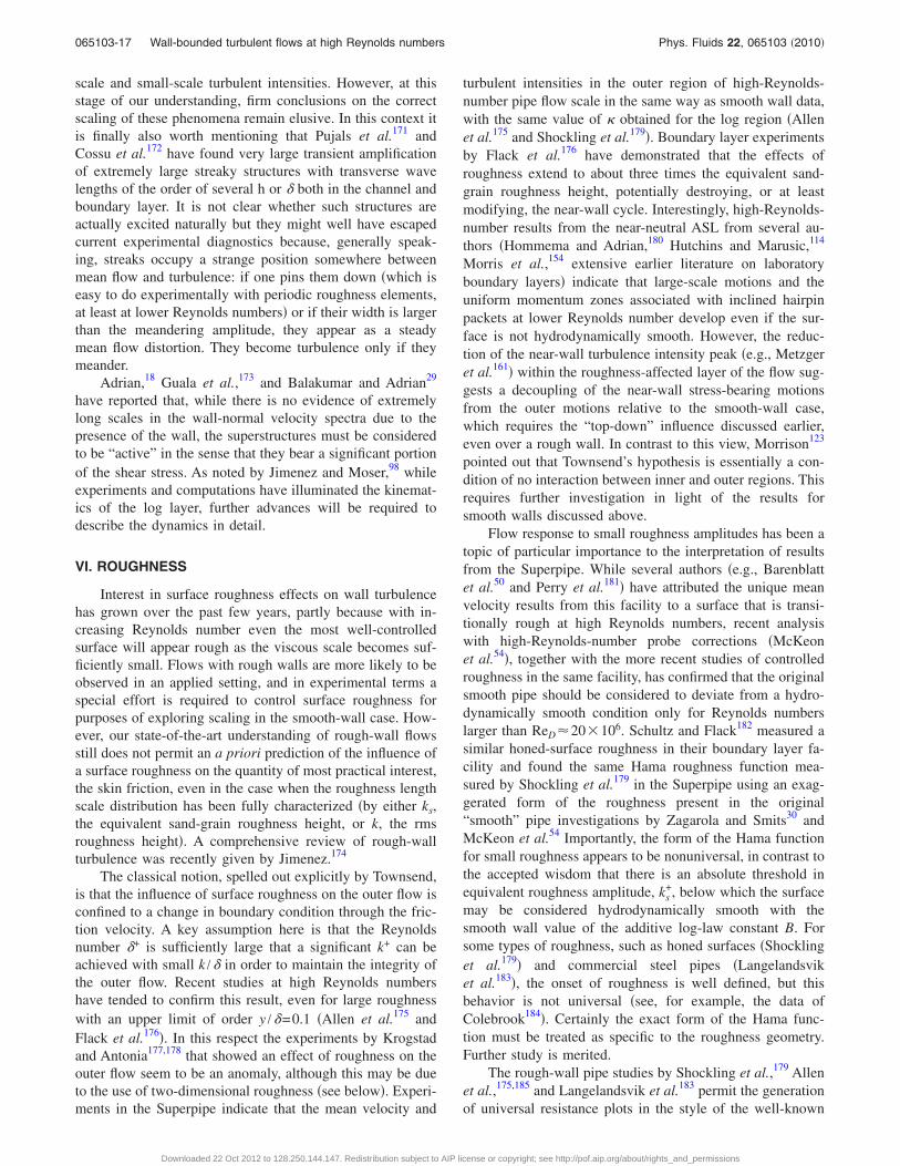
scale and small-scale turbulent intensities. However, at thisstage of our understanding, firm conclusions on the correctscaling of these phenomena remain elusive. In this context itis finally also worth mentioning that Pujals et al.171 andCossu et al.172 have found very large transient amplificationof extremely large streaky structures with transverse wavelengths of the order of several h or � both in the channel andboundary layer. It is not clear whether such structures areactually excited naturally but they might well have escapedcurrent experimental diagnostics because, generally speak-ing, streaks occupy a strange position somewhere betweenmean flow and turbulence: if one pins them down �which iseasy to do experimentally with periodic roughness elements,at least at lower Reynolds numbers� or if their width is largerthan the meandering amplitude, they appear as a steadymean flow distortion. They become turbulence only if theymeander.

Adrian,18 Guala et al.,173 and Balakumar and Adrian29

have reported that, while there is no evidence of extremelylong scales in the wall-normal velocity spectra due to thepresence of the wall, the superstructures must be consideredto be “active” in the sense that they bear a significant portionof the shear stress. As noted by Jimenez and Moser,98 whileexperiments and computations have illuminated the kinemat-ics of the log layer, further advances will be required todescribe the dynamics in detail.

VI. ROUGHNESS

Interest in surface roughness effects on wall turbulencehas grown over the past few years, partly because with in-creasing Reynolds number even the most well-controlledsurface will appear rough as the viscous scale becomes suf-ficiently small. Flows with rough walls are more likely to beobserved in an applied setting, and in experimental terms aspecial effort is required to control surface roughness forpurposes of exploring scaling in the smooth-wall case. How-ever, our state-of-the-art understanding of rough-wall flowsstill does not permit an a priori prediction of the influence ofa surface roughness on the quantity of most practical interest,the skin friction, even in the case when the roughness lengthscale distribution has been fully characterized �by either ks,the equivalent sand-grain roughness height, or k, the rmsroughness height�. A comprehensive review of rough-wallturbulence was recently given by Jimenez.174

The classical notion, spelled out explicitly by Townsend,is that the influence of surface roughness on the outer flow isconfined to a change in boundary condition through the fric-tion velocity. A key assumption here is that the Reynoldsnumber �+ is sufficiently large that a significant k+ can beachieved with small k /� in order to maintain the integrity ofthe outer flow. Recent studies at high Reynolds numbershave tended to confirm this result, even for large roughnesswith an upper limit of order y /�=0.1 �Allen et al.175 andFlack et al.176�. In this respect the experiments by Krogstadand Antonia177,178 that showed an effect of roughness on theouter flow seem to be an anomaly, although this may be dueto the use of two-dimensional roughness �see below�. Experi-ments in the Superpipe indicate that the mean velocity and

turbulent intensities in the outer region of high-Reynolds-number pipe flow scale in the same way as smooth wall data,with the same value of � obtained for the log region �Allenet al.175 and Shockling et al.179�. Boundary layer experimentsby Flack et al.176 have demonstrated that the effects ofroughness extend to about three times the equivalent sand-grain roughness height, potentially destroying, or at leastmodifying, the near-wall cycle. Interestingly, high-Reynolds-number results from the near-neutral ASL from several au-thors �Hommema and Adrian,180 Hutchins and Marusic,114

Morris et al.,154 extensive earlier literature on laboratoryboundary layers� indicate that large-scale motions and theuniform momentum zones associated with inclined hairpinpackets at lower Reynolds number develop even if the sur-face is not hydrodynamically smooth. However, the reduc-tion of the near-wall turbulence intensity peak �e.g., Metzgeret al.161� within the roughness-affected layer of the flow sug-gests a decoupling of the near-wall stress-bearing motionsfrom the outer motions relative to the smooth-wall case,which requires the “top-down” influence discussed earlier,even over a rough wall. In contrast to this view, Morrison123

pointed out that Townsend’s hypothesis is essentially a con-dition of no interaction between inner and outer regions. Thisrequires further investigation in light of the results forsmooth walls discussed above.

Flow response to small roughness amplitudes has been atopic of particular importance to the interpretation of resultsfrom the Superpipe. While several authors �e.g., Barenblattet al.50 and Perry et al.181� have attributed the unique meanvelocity results from this facility to a surface that is transi-tionally rough at high Reynolds numbers, recent analysiswith high-Reynolds-number probe corrections �McKeonet al.54�, together with the more recent studies of controlledroughness in the same facility, has confirmed that the originalsmooth pipe should be considered to deviate from a hydro-dynamically smooth condition only for Reynolds numberslarger than ReD�20�106. Schultz and Flack182 measured asimilar honed-surface roughness in their boundary layer fa-cility and found the same Hama roughness function mea-sured by Shockling et al.179 in the Superpipe using an exag-gerated form of the roughness present in the original“smooth” pipe investigations by Zagarola and Smits30 andMcKeon et al.54 Importantly, the form of the Hama functionfor small roughness appears to be nonuniversal, in contrast tothe accepted wisdom that there is an absolute threshold inequivalent roughness amplitude, ks

+, below which the surfacemay be considered hydrodynamically smooth with thesmooth wall value of the additive log-law constant B. Forsome types of roughness, such as honed surfaces �Shocklinget al.179� and commercial steel pipes �Langelandsviket al.183�, the onset of roughness is well defined, but thisbehavior is not universal �see, for example, the data ofColebrook184�. Certainly the exact form of the Hama func-tion must be treated as specific to the roughness geometry.Further study is merited.

The rough-wall pipe studies by Shockling et al.,179 Allenet al.,175,185 and Langelandsvik et al.183 permit the generationof universal resistance plots in the style of the well-known



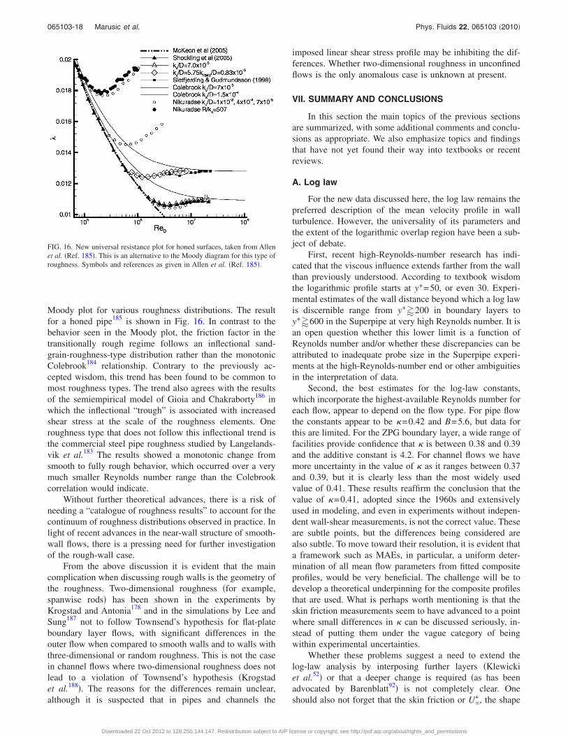
Moody plot for various roughness distributions. The resultfor a honed pipe185 is shown in Fig. 16. In contrast to thebehavior seen in the Moody plot, the friction factor in thetransitionally rough regime follows an inflectional sand-grain-roughness-type distribution rather than the monotonicColebrook184 relationship. Contrary to the previously ac-cepted wisdom, this trend has been found to be common tomost roughness types. The trend also agrees with the resultsof the semiempirical model of Gioia and Chakraborty186 inwhich the inflectional “trough” is associated with increasedshear stress at the scale of the roughness elements. Oneroughness type that does not follow this inflectional trend isthe commercial steel pipe roughness studied by Langelands-vik et al.183 The results showed a monotonic change fromsmooth to fully rough behavior, which occurred over a verymuch smaller Reynolds number range than the Colebrookcorrelation would indicate.

Without further theoretical advances, there is a risk ofneeding a “catalogue of roughness results” to account for thecontinuum of roughness distributions observed in practice. Inlight of recent advances in the near-wall structure of smooth-wall flows, there is a pressing need for further investigationof the rough-wall case.

From the above discussion it is evident that the maincomplication when discussing rough walls is the geometry ofthe roughness. Two-dimensional roughness �for example,spanwise rods� has been shown in the experiments byKrogstad and Antonia178 and in the simulations by Lee andSung187 not to follow Townsend’s hypothesis for flat-plateboundary layer flows, with significant differences in theouter flow when compared to smooth walls and to walls withthree-dimensional or random roughness. This is not the casein channel flows where two-dimensional roughness does notlead to a violation of Townsend’s hypothesis �Krogstadet al.188�. The reasons for the differences remain unclear,although it is suspected that in pipes and channels the

imposed linear shear stress profile may be inhibiting the dif-ferences. Whether two-dimensional roughness in unconfinedflows is the only anomalous case is unknown at present.

VII. SUMMARY AND CONCLUSIONS

In this section the main topics of the previous sectionsare summarized, with some additional comments and conclu-sions as appropriate. We also emphasize topics and findingsthat have not yet found their way into textbooks or recentreviews.

A. Log law

For the new data discussed here, the log law remains thepreferred description of the mean velocity profile in wallturbulence. However, the universality of its parameters andthe extent of the logarithmic overlap region have been a sub-ject of debate.

First, recent high-Reynolds-number research has indi-cated that the viscous influence extends farther from the wallthan previously understood. According to textbook wisdomthe logarithmic profile starts at y+=50, or even 30. Experi-mental estimates of the wall distance beyond which a log lawis discernible range from y+�200 in boundary layers toy+�600 in the Superpipe at very high Reynolds number. It isan open question whether this lower limit is a function ofReynolds number and/or whether these discrepancies can beattributed to inadequate probe size in the Superpipe experi-ments at the high-Reynolds-number end or other ambiguitiesin the interpretation of data.

Second, the best estimates for the log-law constants,which incorporate the highest-available Reynolds number foreach flow, appear to depend on the flow type. For pipe flowthe constants appear to be �=0.42 and B=5.6, but data forthis are limited. For the ZPG boundary layer, a wide range offacilities provide confidence that � is between 0.38 and 0.39and the additive constant is 4.2. For channel flows we havemore uncertainty in the value of � as it ranges between 0.37and 0.39, but it is clearly less than the most widely usedvalue of 0.41. These results reaffirm the conclusion that thevalue of �=0.41, adopted since the 1960s and extensivelyused in modeling, and even in experiments without indepen-dent wall-shear measurements, is not the correct value. Theseare subtle points, but the differences being considered arealso subtle. To move toward their resolution, it is evident thata framework such as MAEs, in particular, a uniform deter-mination of all mean flow parameters from fitted compositeprofiles, would be very beneficial. The challenge will be todevelop a theoretical underpinning for the composite profilesthat are used. What is perhaps worth mentioning is that theskin friction measurements seem to have advanced to a pointwhere small differences in � can be discussed seriously, in-stead of putting them under the vague category of beingwithin experimental uncertainties.

Whether these problems suggest a need to extend thelog-law analysis by interposing further layers �Klewickiet al.52� or that a deeper change is required �as has beenadvocated by Barenblatt92� is not completely clear. Oneshould also not forget that the skin friction or U�

+, the shape

FIG. 16. New universal resistance plot for honed surfaces, taken from Allenet al. �Ref. 185�. This is an alternative to the Moody diagram for this type ofroughness. Symbols and references as given in Allen et al. �Ref. 185�.



factor H, and the streamwise boundary layer growth ��x�are intimately tied to the parameters of the mean flow profile�Monkewitz et al.49� and therefore provide useful cross-checks on consistency. Similarly, in internal flows, consis-tency is required between the mean flow parameters and theprofiles in inner and outer scaling, the centerline velocity, thefriction factor, etc. �McKeon et al.54�. Additional high-Reynolds-number experiments, and even more accurate skinfriction data, would be valuable in these regards. If the loglaw is indeed the proper asymptotic solution, determining thevon Kármán “constant” from first principles represents agrand challenge for our field. Having different values of �for ZPG boundary layers, pipe, and channel flows presents asignificant challenge for turbulence models, as well astheory.

B. Relation between inner and outer scaling

Evidence of outer-scale contributions to the near-wallregion has been noted since the study of Rao et al.,164 whodocumented that large outer-scaled structures were active inrearranging and interacting with near-wall structure, and con-sequently influencing the “bursting” frequency. Recent stud-ies show that such inner-outer interactions become more evi-dent with increasing Reynolds number, particularly for thestreamwise component of turbulence intensity. This contra-dicts wall-scaling approaches that assume all inner regionstatistics to scale exclusively on inner variables. While thelocation of the near-wall peak of u2+ scales with inner vari-ables, in boundary layers there is a clear trend of increasingmagnitude with Reynolds number. On the other hand, thespacing of near-wall streaks is found to be independent ofReynolds number over a very wide range when scaled oninner variables. Mixed scaling �a geometric mean of innerand outer scales� does not seem to provide a physicallymeaningful scaling parameter given the complexity of theinteractions. Present data also suggest that the peaks in w2+,and possibly in v2+, change with Reynolds number in loca-tion and value �as previously reported by Sreenivasan15�. De-spite the uncertainties of present data, it is difficult to escapethe conclusion that different components of the Reynoldsstress tensor scale differently. This poses a problem of math-ematical consistency as one expects a tensor to scale as awhole. A “way out” may be the concept of block matching�Crighton and Leppington189� in MAE in which all the termswith the same power of the small parameter � multiplied byany power of ln�� are considered to be of the same order.Applied to the Reynolds stress tensor, a slow growth of someof its components as lnn�R� would be mathematically de-scribable. It is increasingly likely that for each inner �outer�quantity there exists an essentially inner �outer� scalingmodulated by some weak function of Reynolds number, andthe extent of this modulation will depend on the quantity thatis being considered. Again, these issues will remain openuntil detailed measurements are carried out over a range ofReynolds numbers up to some very high value and/or a co-herent theoretical framework is put forward.

C. Turbulence structure

We noted three basic eddy motions: near-wall streaks,which have been shown to follow inner scaling, the LSMs,which are related to outer layer bulges and the vortex packetsas discussed by Head and Bandyophadyay12 and Adrian,18

and the VLSMs interpreted by Adrian and coworkers interms of concatenated packets of vortices and by Marusicand coworkers in terms of the meandering superstructures.Separation of the latter two structure types is nontrivial sincetheir very nature dictates that Taylor’s hypothesis cannot beappropriate as a diagnostic tool. Although this conclusion hasbeen widely accepted in the past, recent measurements in thenear-wall region have added significance to this observation.An important consequence of the interaction between thesestructures is observed via the Reynolds-number-dependentpeak of the streamwise intensity in the inner layer �neary+=12–15�.

While large streamwise structures in wall turbulencehave been documented for many decades �Townsend4 andKovazsnay et al.190�, the dynamical importance of the largeststructures �VLSM� had not been appreciated until recently.For example, the low wavenumber VLSMs appear to con-tribute about half of the total energy of the streamwise tur-bulence component at high Reynolds number. Also, they donot appear to scale with outer layer variables as assumed inthe Perry–Townsend attached eddy model. What is clear isthat differing views exist and many open questions remainregarding the VLSM/superstructures. One key question con-cerns their scaling. If they depend on the scale of the appa-ratus, it suggests the disturbing and profound possibility thatit is not possible to realize a facility-independent asymptoticstate of turbulence �even for fully developed internal flows,such as pipes and channels�.

The role of the turbulence structure relates directly to thespectral scaling laws. While kx

−5/3 scaling in the spectrum ofthe streamwise component is well established, experimentsnow indicate that the kx

−1 region is only evident at very highReynolds numbers over a very limited wave-number range.Although the interactions between outer layer motions andinner layer motions have become much clearer in recentyears, the simple division between inner and outer layer scal-ing that leads to the kx

−1 region fails to capture those interac-tions. Specifically, the region where we might expect kx

−1

scaling corresponds to the wave numbers occupied by theLSMs, and experiments have shown that although the LSMsappear to behave as attached motions, they do not scale sim-ply on wall variables.

D. Boundary layers versus pipes/channels

We mentioned the puzzle as to whether the von Kármánconstant � is different in pipes, channels, and boundary lay-ers. Other differences have also been highlighted betweenboundary layer flows and the confined flows of pipes andchannels. This extends beyond the well-documented and ob-vious differences in the outermost region and includes theinner-scaled streamwise turbulence intensity and the othercomponents of Reynolds stress, which may be subtly differ-ent between these flows even in the viscous buffer region.



Recent studies �Jimenez and Hoyas126 and Buschmannet al.137� report significant differences for the available w2+

and v2+ profiles between boundary layers and internal flowsin the logarithmic region. These measurements are sparse�and difficult to obtain� at high Reynolds numbers, and fur-ther work is warranted. Note, however, that all these findingsare consistent with the inner region being influenced byouter-scale motions, which have been shown to depend onthe outer geometry.

It has become clear that the relative importance of LSMsand VLSMs depends on the nature of the flow: they appearto behave differently in pipes, channels, and boundary layers�Hutchins and Marusic,114 Bailey et al.,157 and Montyet al.155�. Monty et al.155 concluded that superstructures asreported by Hutchins and Marusic114 in boundary layers aredifferent from the VSLMs reported by Kim and Adrian26 inpipe and channel flows. Whether the quantitative differencesobserved are due to the interaction with the opposite wall inpipe and channel flows or the intermittency of the outer re-gion in boundary layers remains uncertain. Another issuewhich complicates comparisons is the appropriate Reynoldsnumber for comparison.

E. Roughness

Recent high-Reynolds-number experiments have broadlyupheld Townsend’s hypothesis that the influence of rough-ness on the outer region is restricted solely to changing theboundary condition, U�. This is found to be so even for largeroughness elements, despite their influence extending toabout three times their height from the wall. However,anomalous experiments do exist, particularly with two-dimensional roughness in boundary layers, and these willneed to be explained.

New roughness experiments have shown that most �butnot all� roughness types produce an inflectional �Nikuradse-like� transitional resistance relationship. While Nikuradse’sresults in rough-wall flows are for the specific sand-grainroughness, they are far more representative of the practicalconditions than any of the Colebrook correlations, which aresmoothed curves through a variety of practical conditions,but not accurately representative of any of them. This impliesthat schemes based on Colebrook’s interpolation �such as theMoody diagram� have to be phased out gracefully.

F. Experimental methods

The past couple of decades have seen a number of high-Reynolds-number facilities come on line �including all thefacilities cited in Table I�, with others on the way �CICLoPEand the New Hampshire tunnel�. We now recognize that in-dependent measurements of the wall shear stress in allboundary layers �and most channel flows� are essential, withthe fully developed pipe flow being the exception. The valueof any data is greatly diminished without such independentaccompanying measurements. Existing facilities �particularlythe channel and pipe flows at Melbourne� have helped toimprove our understanding of flow development in fully de-veloped flows.

We also now have a much better appreciation of the

effects of initial conditions on boundary layers �from experi-ments and from DNS�. Because boundary layers are gener-ated in flow facilities in many different ways, for instance, onwalls of test sections or on suspended plates, with differentstarting conditions and different devices to achieve the fullyturbulent state, the virtual origin of the turbulent boundarylayer can vary a great deal. While it is most convenient inpractice to correlate the local skin friction with a Reynoldsnumber based on x, such correlations are of very limited useor general validity. The new derivation of streamwise bound-ary layer growth from the log law and the basic equationshas brought about a significant improvement as the virtualorigin of ZPG TBLs can now be determined from localintegral parameters without the need for additional fittingparameters.

The ASL has proven to be an invaluable and single re-source for extremely high-Reynolds-number data, while atthe same time we recognize clearly its limitations for provid-ing high quality data and continue to debate its suitability asa model for the canonical case.

We have highlighted the effects of spatial resolution onhot-wire response, which is much more pervasive than pre-viously thought. The development of very small probes tosolve this problem for existing facilities is under way andfuture facilities are generally being designed to overcome thespatial resolution problem by building them on a largeenough scale. We have also seen the development of newinstrumentation to measure pressure fluctuations within a tur-bulent flow with good spatial resolution.

G. Modeling and prediction

Nearly all turbulence models, and their computationalimplementations for the prediction of wall-bounded flows,depend explicitly or implicitly on the overlap region param-eters. Therefore, all of the issues raised above have a sub-stantial impact on our ability to predict such flows, in par-ticular, for complex flow fields or geometries. For example,the sensitivity of the results to the von Kármán constantalone can lead to unacceptable errors in predictions. Simplyrelying on calibration of the many coefficients used in thesemodels, which are specific to particular flow geometriesover limited ranges of Reynolds number, is not a prudentapproach.

VIII. CLOSING REMARKS

Significant work has been carried out over the past de-cade on wall-bounded turbulence, and this has largely beendriven by the desire to generate data at high Reynolds num-bers; DNSs have proceeded in a similar way. Even so, manyof the outstanding issues listed by Sreenivasan15 20 yearsago remain open, and, indeed, new experiments have led tonew questions related to scaling laws and the role of thelargest scale motions. At the moment, extracting a theory bysifting through the data more carefully is the missing ele-ment. A positive development is that, perhaps more than everbefore, we are starting to develop extensive collaborations,sharing facilities, instrumentation, and ideas. These effortsare likely to be increasingly international and cooperative.



One project, inspired by the workshops and already underway, called ICET �International Collaboration on Experi-ments in Turbulence� is an attempt to explore the limits ofturbulent flow facilities and their instrumentation by a groupof scientists drawn from Australia, Italy, Japan, Sweden,Switzerland, and the United States, with experiments carriedout jointly in wind tunnels at Stockholm, Melbourne, andChicago, listed in Table I. Such efforts, and others in thefuture, are indeed required for a better understanding of high-Reynolds-number turbulence.

ACKNOWLEDGMENTS

We wish to thank all of our colleagues who have con-tributed to the International Workshop series with their par-ticipation and various communications. The InternationalCenter for Theoretical Physics, Trieste, and the EttoreMajorano Foundation and Center for Scientific Culture,Erice, are gratefully acknowledged for their financial andmanagerial support of the 2004 and 2006 workshops, respec-tively. The financial support of the Australian ResearchCouncil �I.M.�, the National Science Foundation �B.J.M. andA.J.S.�, and the Office of Naval Research �A.J.S.� is alsogratefully acknowledged.

1F. H. Clauser, “The turbulent boundary layer,” Adv. Mech. 4, 1 �1956�.2D. E. Coles and E. A. Hirst, Proceedings of the Computation of TurbulentBoundary Layers, AFOSR-IFP-Stanford Conference 1968 �Stanford Uni-versity, Stanford, 1969�, Vol. II.

3M. Gad-el-Hak and P. Bandyopadhyay, “Reynolds number effects in wall-bounded turbulent flows,” Appl. Mech. Rev. 47, 307 �1994�.

4A. A. Townsend, The Structure of Turbulent Shear Flow �Cambridge Uni-versity Press, Cambridge, 1956�.

5A. A. Townsend, The Structure of Turbulent Shear Flow, 2nd ed. �Cam-bridge University Press, Cambridge, 1976�.

6D. E. Coles, “The law of the wake in the turbulent boundary layer,” J.Fluid Mech. 1, 191 �1956�.

7J. C. Rotta, “Turbulent boundary layers in incompressible flow,” Prog.Aerosp. Sci. 2, 1 �1962�.

8C. M. Millikan, Proceedings of the Fifth International Congress On Ap-plied Mechanics �Wiley, New York, 1938�.

9T. Theodorsen, Proceedings of the Second Midwestern Conference onFluid Mechanics, 17–19 March �Ohio State University, Columbus, OH,1952�.

10F. R. Hama, J. D. Long, and J. C. Hegarty, “On transition from laminar toturbulent flow,” J. Appl. Phys. 28, 388 �1957�.

11S. J. Kline, W. C. Reynolds, F. A. Schraub, and P. W. Rundstadler, “Thestructure of turbulent boundary layers,” J. Fluid Mech. 30, 741 �1967�.

12M. R. Head and P. R. Bandyopadhyay, “New aspects of turbulent struc-ture,” J. Fluid Mech. 107, 297 �1981�.

13A. E. Perry and M. S. Chong, “On the mechanism of wall turbulence,” J.Fluid Mech. 119, 173 �1982�.

14B. J. Cantwell, “Organised motion in turbulent flow,” Annu. Rev. FluidMech. 13, 457 �1981�.

15K. R. Sreenivasan, in Frontiers in Experimental Fluid Mechanics, editedby M. Gad el Hak �Springer-Verlag, New York, 1989�.

16S. K. Robinson, “Coherent motions in turbulent boundary layers,” Annu.Rev. Fluid Mech. 23, 601 �1991�.

17R. L. Panton, “Overview of the self-sustaining mechanisms of wall turbu-lence,” Prog. Aerosp. Sci. 37, 341 �2001�.

18R. J. Adrian, “Hairpin vortex organization in wall turbulence,” Phys. Flu-ids 19, 041301 �2007�.

19P. Bradshaw, “The turbulence structure of equilibrium boundary layers,” J.Fluid Mech. 29, 625 �1967�.

20I. Marusic and G. J. Kunkel, “Streamwise turbulence intensity formulationfor flat-plate boundary layers,” Phys. Fluids 15, 2461 �2003�.

21M. M. Metzger and J. C. Klewicki, “A comparative study of near-wallturbulence in high and low Reynolds number boundary layers,” Phys.Fluids 13, 692 �2001�.

22J. F. Morrison, B. J. McKeon, W. Jiang, and A. J. Smits, “Scaling of thestreamwise velocity component in turbulent pipe flow,” J. Fluid Mech.508, 99 �1999�.

23H. H. Fernholz and P. J. Finley, “The incompressible zero-pressure-gradient turbulent boundary layer: An assessment of the data,” Prog.Aerosp. Sci. 32, 245 �1996�.

24C. R. Smith and S. P. Metzler, “The characteristics of low-speed streaks inthe near-wall region of a turbulent boundary layer,” J. Fluid Mech. 129,27 �1983�.

25J. C. Klewicki, M. M. Metzger, E. Kelner, and E. M. Thurlow, “Viscoussublayer flow visualizations at R �1500000,” Phys. Fluids 7, 857 �1995�.

26K. C. Kim and R. J. Adrian, “Very large-scale motion in the outer layer,”Phys. Fluids 11, 417 �1999�.

27B. J. McKeon and J. F. Morrison, “Asymptotic scaling in turbulent pipeflow,” Philos. Trans. R. Soc. London, Ser. A 365, 771 �2007�.

28I. Marusic, “On the role of large-scale structures in wall turbulence,” Phys.Fluids 13, 735 �2001�.

29B. J. Balakumar and R. J. Adrian, “Large- and very-large scale motions inchannel and boundary-layer flows,” Proc. R. Soc. London, Ser. A 365,665 �2007�.

30M. V. Zagarola and A. J. Smits, “Mean-flow scaling of turbulent pipeflow,” J. Fluid Mech. 373, 33 �1998�.

31J. C. Klewicki, J. F. Foss, and J. M. Wallace, in Flow at Ultra-HighReynolds and Rayleigh Numbers, edited by R. J. Donnelly and K. R.Sreenivasan �Springer, New York, 1998�.

32H. M. Nagib, K. A. Chauhan, and P. A. Monkewitz, “Approach to anasymptotic state for zero pressure gradient turbulent boundary layers,”Philos. Trans. R. Soc. London, Ser. A 365, 755 �2007�.

33J. M. Österlund, A. V. Johansson, H. M. Nagib, and M. H. Hites, “A noteon the overlap region in turbulent boundary layers,” Phys. Fluids 12, 1�2000�.

34J. Carlier and M. Stanislas, “Experimental study of eddy structures in aturbulent boundary layer using particle image velocimetry,” J. Fluid Mech.535, 143 �2005�.

35T. B. Nickels, I. Marusic, S. M. Hafez, and M. S. Chong, “Evidence of thek−1 law in a high-Reynolds-number turbulent boundary layer,” Phys. Rev.Lett. 95, 074501 �2005�.

36D. B. De Graaff and J. K. Eaton, “Reynolds-number scaling of the flat-plate turbulent boundary layer,” J. Fluid Mech. 422, 319 �2000�.

37R. J. Adrian, C. D. Meinhart, and C. D. Tomkins, “Vortex organization inthe outer region of the turbulent boundary layer,” J. Fluid Mech. 422, 1�2000�.

38C. D. Tomkins and R. J. Adrian, “Spanwise structure and scale growth inturbulent boundary layers,” J. Fluid Mech. 490, 37 �2003�.

39C. J. Kähler, “Investigation of the spatio-temporal flow structure in thebuffer region of a turbulent boundary layer by means of multiple planestereo PIV,” Exp. Fluids 36, 114 �2004�.

40B. Ganapathisubramani, E. K. Longmire, and I. Marusic, “Characteristicsof vortex packets in turbulent boundary layers,” J. Fluid Mech. 478, 35�2003�.

41W. T. Hambleton, N. Hutchins, and I. Marusic, “Simultaneous orthogonal-plane particle image velocimetry measurements in a turbulent boundarylayer,” J. Fluid Mech. 560, 53 �2006�.

42G. E. Elsinga, R. J. Adrian, B. W. van Oudheusden, and F. Scarano,Seventh International Symposium on Particle Image Velocimetry, Rome,Italy, 2007 �Sapienza University of Rome, Rome, 2007�.

43R. D. Moser, J. Kim, and N. N. Mansour, “Direct numerical simulation ofturbulent channel flow up to R�=590,” Phys. Fluids 11, 943 �1999�.

44H. Abe, H. Kawamura, and H. Choi, “Very large-scale structures and theireffects on the wall shear-stress fluctuations in a turbulent channel flow upto Re�=640,” J. Fluids Eng. 126, 835 �2004�.

45K. Iwamoto, T. Tsukahara, H. Nakano, and H. Kawamura, in IUTAMSymposium on Computational Physics and New Perspectives in Turbu-lence, edited by Y. Kaneda �Springer, New York, 2006�, pp. 53–58.

46J. C. del Álamo, J. Jiménez, P. Zandonade, and R. D. Moser, “Self-similarvortex clusters in the turbulent logarithmic region,” J. Fluid Mech. 561,329 �2006�.

47S. Hoyas and J. Jiménez, “Scaling of the velocity fluctuations in turbulentchannels up to Re�=2003,” Phys. Fluids 18, 011702 �2006�.



http://dx.doi.org/10.1016/S0065-2156(08)70370-3

http://dx.doi.org/10.1115/1.3111083

http://dx.doi.org/10.1017/S0022112056000135

http://dx.doi.org/10.1017/S0022112056000135

http://dx.doi.org/10.1016/0376-0421(62)90014-3

http://dx.doi.org/10.1016/0376-0421(62)90014-3

http://dx.doi.org/10.1063/1.1722760

http://dx.doi.org/10.1017/S0022112067001740

http://dx.doi.org/10.1017/S0022112081001791

http://dx.doi.org/10.1017/S0022112082001311

http://dx.doi.org/10.1017/S0022112082001311

http://dx.doi.org/10.1146/annurev.fl.13.010181.002325




http://dx.doi.org/10.1016/S0376-0421(01)00009-4

http://dx.doi.org/10.1063/1.2717527

http://dx.doi.org/10.1063/1.2717527

http://dx.doi.org/10.1017/S0022112067001089

http://dx.doi.org/10.1017/S0022112067001089

http://dx.doi.org/10.1063/1.1589014

http://dx.doi.org/10.1063/1.1344894

http://dx.doi.org/10.1063/1.1344894

http://dx.doi.org/10.1017/S0022112004008985

http://dx.doi.org/10.1016/0376-0421(95)00007-0

http://dx.doi.org/10.1016/0376-0421(95)00007-0

http://dx.doi.org/10.1017/S0022112083000634

http://dx.doi.org/10.1063/1.868763

http://dx.doi.org/10.1063/1.869889

http://dx.doi.org/10.1098/rsta.2006.1945

http://dx.doi.org/10.1063/1.1343480

http://dx.doi.org/10.1063/1.1343480

http://dx.doi.org/10.1017/S0022112098002419


http://dx.doi.org/10.1063/1.870250

http://dx.doi.org/10.1017/S0022112005004751

http://dx.doi.org/10.1103/PhysRevLett.95.074501


http://dx.doi.org/10.1017/S0022112000001713

http://dx.doi.org/10.1017/S0022112000001580

http://dx.doi.org/10.1017/S0022112003005251

http://dx.doi.org/10.1007/s00348-003-0680-3

http://dx.doi.org/10.1017/S0022112002003270

http://dx.doi.org/10.1017/S0022112006000292

http://dx.doi.org/10.1063/1.869966

http://dx.doi.org/10.1115/1.1789528

http://dx.doi.org/10.1017/S0022112006000814

http://dx.doi.org/10.1063/1.2162185

48Z. Hu, C. Morley, and N. Sandman, “Wall pressure and shear stress spec-tra from direct simulations of channel flow,” AIAA J. 44, 1541 �2006�.

49P. A. Monkewitz, K. A. Chauhan, and H. M. Nagib, “Self-contained high-Reynolds-number asymptotics for zero-pressure-gradient turbulent bound-ary layers,” Phys. Fluids 19, 115101 �2007�.

50G. I. Barenblatt, A. J. Chorin, O. H. Hald, and V. M. Prostokishin, “Struc-ture of the zero-pressure-gradient turbulent boundary layer,” Proc. Natl.Acad. Sci. U.S.A. 94, 7817 �1997�.

51W. K. George and L. Castillo, “Zero-pressure-gradient turbulent boundarylayer,” Appl. Mech. Rev. 50, 689 �1997�.

52J. C. Klewicki, P. Fife, T. Wei, and P. McMurtry, “A physical model of theturbulent boundary layer consonant with mean momentum balance struc-ture,” Philos. Trans. R. Soc. London, Ser. A 365, 823 �2007�.

53B. J. McKeon and K. R. Sreenivasan, “Introduction: Scaling and structurein high Reynolds number wall-bounded flows,” Philos. Trans. R. Soc.London, Ser. A 365, 635 �2007�.

54B. J. McKeon, J. Li, W. Jiang, J. F. Morrison, and A. J. Smits, “Furtherobservations on the mean velocity distribution in fully developed pipeflow,” J. Fluid Mech. 501, 135 �1999�.

55J. P. Monty, “Developments in smooth wall turbulent duct flows,” Ph.D.thesis, University of Melbourne, 2005.

56E.-S. Zanoun, F. Durst, and H. Nagib, “Evaluating the law of the wall intwo-dimensional fully developed turbulent channel flows,” Phys. Fluids10, 1 �2003�.

57T. B. Nickels, I. Marusic, S. M. Hafez, N. Hutchins, and M. S. Chong,“Some predictions of the attached eddy model for a high Reynolds numberboundary layer,” Philos. Trans. R. Soc. London, Ser. A 365, 807 �2007�.

58R. Duncan, N. Hutchins, J. Monty, and A. Segalini, APS/DFD Meeting,2009 �University of Minnesota, Minneapolis, 2009�.

59A. Talamelli, F. Persiani, J. H. M. Fransson, H. Alfredsson, A. V.Johansson, H. M. Nagib, J. D. Ruedi, K. R. Sreenivasan, and P. A.Monkewitz, “CICLoPE—A response to the need for high Reynolds num-ber experiments,” Fluid Dyn. Res. 41, 021407 �2009�.

60J. C. Klewicki, private communication.61M. Metzger, “Scalar dispersion in high Reynolds number turbulent bound-

ary layers,” Ph.D. thesis, University of Utah, 2002.62I. Marusic and N. Hutchins, “Study of the log-layer structure in wall

turbulence over a very large range of Reynolds number,” Flow, Turbul.Combust. 81, 115 �2008�.

63J. C. Klewicki, P. J. A. Priyadarshana, and M. M. Metzger, “Statisticalstructure of the fluctuating wall pressure and its in-plane gradients at highReynolds number,” J. Fluid Mech. 609, 195 �2008�.

64J. D. Ruedi, H. M. Nagib, J. Osterlund, and P. A. Monkewitz, “Evaluationof three techniques for wall-shear measurements in three-dimensionalflows,” Exp. Fluids 35, 389 �2003�.

65H. H. Fernholz, G. Janke, M. Schober, P. M. Wagner, and D. Warnack,“New developments and applications of skin-friction measuring tech-niques,” Meas. Sci. Technol. 7, 1396 �1996�.

66J. Nikuradse, “Gesetzimassen der turbuleuten Stromung in glattenRohren,” VDI-Forschungsh. 356, 289 �1932�.

67A. E. Perry, S. M. Henbest, and M. S. Chong, “A theoretical and experi-mental study of wall turbulence,” J. Fluid Mech. 165, 163 �1986�.

68J. Doherty, P. Ngan, J. P. Monty, and M. S. Chong, in Proceedings of the16th Australasian Fluid Mechanics Conference, edited by P. A. Jacobs, T.J. McIntyre, M. J. Cleary, D. Buttsworth, D. J. Mee, R. Clements, R. G.Morgan, and C. Lemckert, University of Queensland, 2007 �The Univer-sity of Queensland, Brisbane, 2007�, pp. 266–270.

69K. Lien, J. P. Monty, M. S. Chong, and A. Ooi, Proceedings of the 15thAustralasian Fluid Mechanics Conference, 2004 �The University of Syd-ney, Sydney, 2004�.

70E.-S. Zanoun, H. M. Nagib, and F. Durst, “Refined Cf relation for turbu-lent channels and consequences for high Re experiments,” Fluid Dyn. Res.41, 021405 �2009�.

71X. Wu and P. Moin, “A direct numerical simulation study on the meanvelocity characteristics in turbulent pipe flow,” J. Fluid Mech. 608, 81�2008�.

72R. Narasimha and A. Prabhu, “Equlibrium and relaxation in turbulentwakes,” J. Fluid Mech. 54, 1 �1972�.

73M. B. Jones, I. Marusic, and A. E. Perry, “Evolution and structure of sinkflow turbulent boundary layers,” J. Fluid Mech. 428, 1 �2001�.

74D. E. Coles, “The turbulent boundary layer in a compressible field,”USAF The Rand Cooperation Technical Report No. R-403-PR, 1962.

75L. Castillo and T. G. Johansson, “The effects of the upstream conditions

on a low Reynolds number turbulent boundary layer with zero pressuregradient,” J. Turbul. 3, 031 �2002�.

76P. A. Monkewitz, K. A. Chauhan, and H. M. Nagib, “Comparison of meanflow similarity laws in zero pressure gradient turbulent boundary layers,”Phys. Fluids 20, 105102 �2008�.

77K. A. Chauhan and H. M. Nagib, in IUTAM Symposium on ComputationalPhysics and New Perspectives in Turbulence, edited by Y. Kaneda�Springer, New York, 2006�, pp. 177–182.

78L. Castillo and D. J. Walker, “Effect of upstream conditions on the outerflow of turbulent boundary layers,” AIAA J. 40, 1292 �2002�.

79K. A. Chauhan, P. A. Monkewitz, and H. M. Nagib, “Criteria for assessingexperiments in zero pressure gradient boundary layers,” Fluid Dyn. Res.41, 021404 �2009�.

80A. E. Perry, I. Marusic, and J. D. Li, “Wall turbulence closure based onclassical similarity laws and the attached eddy hypothesis,” Phys. Fluids6, 1024 �1994�.

81A. E. Perry, I. Marusic, and M. B. Jones, “On the streamwise evolution ofturbulent boundary layers in arbitrary pressure gradients,” J. Fluid Mech.461, 61 �2002�.

82A. E. Perry, I. Marusic, and M. B. Jones, “New evolution equations forturbulent boundary layers in arbitrary pressure gradients,” Sadhana: Proc.,Indian Acad. Sci. 23, 443 �1998�.

83T. Wei, P. Fife, J. C. Klewicki, and P. McMurtry, “Properties of the meanmomentum balance in turbulent boundary layer, pipe and channel flows,”J. Fluid Mech. 522, 303 �1999�.

84R. R. Long and T. C. Chen, “Experimental evidence for the existence ofthe ‘mesolayer’ in turbulent systems,” J. Fluid Mech. 105, 19 �1981�.

85N. Afzal, “Fully turbulent flow in a pipe-an intermediate layer,” Ing.-Arch.52, 355 �1982�.

86K. R. Sreenivasan, in Turbulence Management and Relaminarization, ed-ited by H. W. Liepmann and R. Narasimha �Springer-Verlag, New York,1987�.

87J. Kevorkian and J. D. Cole, Perturbation Methods in Applied Mathemat-ics �Springer, New York, 1985�.

88M. Wosnik, L. Castillo, and W. K. George, “A theory for turbulent pipeand channel flows,” J. Fluid Mech. 421, 115 �2000�.

89M. Oberlack, “A unified approach for symmetries in plane parallel turbu-lent shear flows,” J. Fluid Mech. 427, 299 �2001�.

90B. Lindgren, J. M. Osterlund, and A. V. Johansson, “Evaluation of scalinglaws derived from Lie group symmetry methods in zero-pressure-gradientturbulent boundary layers,” J. Fluid Mech. 502, 127 �1999�.

91P. R. Spalart, G. R. Coleman, and R. Johnstone, “Direct numerical simu-lation of the Ekman layer: A step in Reynolds number, and cautious sup-port for a log law with a shifted origin,” Phys. Fluids 20, 101507 �2008�.

92G. I. Barenblatt, “Scaling laws for fully developed turbulent shear flows.Part 1. Basic hypotheses and analysis,” J. Fluid Mech. 248, 513 �1993�.

93W. K. George, “Recent advancements toward the understanding of turbu-lent boundary layers,” AIAA J. 44, 2435 �2006�.

94W. K. George, “Is there a universal log law for turbulent wall-boundedflows?” Philos. Trans. R. Soc. London, Ser. A 365, 789 �2007�.

95M. B. Jones, T. B. Nickels, and I. Marusic, “On the asymptotic similarityof the zero pressure-gradient turbulent boundary layer,” J. Fluid Mech.616, 195 �2008�.

96R. L. Panton, “Composite asymptotic expansions and scaling wall turbu-lence,” Philos. Trans. R. Soc. London, Ser. A 365, 733 �2007�.

97B. J. McKeon, “High Reynolds number turbulent pipe flow,” Ph.D. thesis,Princeton University, 2003.

98J. Jiménez and R. D. Moser, “What are we learning from simulating wallturbulence?” Philos. Trans. R. Soc. London, Ser. A 365, 715 �2007�.

99N. Afzal, “Millikan’s argument at moderately large Reynolds number,”Phys. Fluids 19, 600 �1976�.

100K. R. Sreenivasan and A. Sahay, in Self-Sustaining Mechanisms of WallTurbulence, edited by R. Panton �WIT Press, Southampton, 1997�, pp.253–272.

101P. A. Monkewitz and H. M. Nagib, “The Reynolds shear stress in zeropressure gradient turbulent boundary layers derived from log-law asymp-totics,” Bull. Am. Phys. Soc. 53, 97 �2008�.

102K. A. Chauhan, H. M. Nagib, and P. A. Monkewitz, in Progress in Tur-bulence 2. Proceedings of iTi Conference in Turbulence, edited by M.Oberlack, G. Khujadze, S. Guenther, T. Weller, M. Frewer, J. Peinke, andS. Barth �Springer, New York, 2007�, pp. 159–163.

103H. M. Nagib and K. A. Chauhan, “Variations of von Kármán coefficientin canonical flows,” Phys. Fluids 20, 101518 �2008�.



http://dx.doi.org/10.2514/1.17638

http://dx.doi.org/10.1063/1.2780196

http://dx.doi.org/10.1073/pnas.94.15.7817

http://dx.doi.org/10.1073/pnas.94.15.7817

http://dx.doi.org/10.1115/1.3101858




http://dx.doi.org/10.1017/S0022112003007304


http://dx.doi.org/10.1088/0169-5983/41/2/021407

http://dx.doi.org/10.1007/s10494-007-9116-0

http://dx.doi.org/10.1007/s10494-007-9116-0

http://dx.doi.org/10.1017/S0022112008002541

http://dx.doi.org/10.1007/s00348-003-0650-9

http://dx.doi.org/10.1088/0957-0233/7/10/010

http://dx.doi.org/10.1017/S002211208600304X

http://dx.doi.org/10.1088/0169-5983/41/2/021405

http://dx.doi.org/10.1017/S0022112008002085

http://dx.doi.org/10.1017/S0022112072000497

http://dx.doi.org/10.1017/S0022112000002597

http://dx.doi.org/10.1088/1468-5248/3/1/031

http://dx.doi.org/10.1063/1.2972935

http://dx.doi.org/10.2514/2.1818

http://dx.doi.org/10.1088/0169-5983/41/2/021404

http://dx.doi.org/10.1063/1.868336

http://dx.doi.org/10.1017/S002211200200825X

http://dx.doi.org/10.1007/BF02744574

http://dx.doi.org/10.1007/BF02744574

http://dx.doi.org/10.1017/S0022112004001958

http://dx.doi.org/10.1017/S0022112081003108

http://dx.doi.org/10.1007/BF00536208

http://dx.doi.org/10.1017/S0022112000001385

http://dx.doi.org/10.1017/S0022112000002408

http://dx.doi.org/10.1017/S0022112003007675

http://dx.doi.org/10.1063/1.3005858

http://dx.doi.org/10.1017/S0022112093000874

http://dx.doi.org/10.2514/1.19951


http://dx.doi.org/10.1017/S0022112008004205



http://dx.doi.org/10.1063/1.861498

http://dx.doi.org/10.1063/1.3006423

104R. L. Panton, “Review of wall turbulence as described by compositeexpansions,” Appl. Mech. Rev. 58, 1 �2005�.

105P. R. Spalart, “Direct simulation of turbulent boundary layer up toR =1410,” J. Fluid Mech. 187, 61 �1988�.

106H. M. Nagib, C. Christophorou, and P. A. Monkewitz, “High Reynoldsnumber turbulent boundary layers subjected to various pressure-gradientconditions,” in IUTAM Symposium on One Hundred Years of BoundaryLayer Research, DLR Göttingen, Germany, 12–14 August 2004, editedby G. E. A. Meier and K. R. Sreenivasan �Springer, Berlin, 2004�, pp.383–394.

107S. A. Dixit and O. N. Ramesh, “Pressure-gradient-dependent logarithmiclaws in sink flow turbulent boundary layers,” J. Fluid Mech. 615, 445�2008�.

108C. Bourassa and F. O. Thomas, “An experimental investigation of ahighly accelerated turbulent boundary layer,” J. Fluid Mech. 634, 359�2009�.

109F. A. MacMillan, “Experiments on Pitot-tubes in shear flow,” Ministry ofSupply, Aeronautical Research Council Technical Report No. R&M 3028,1956.

110B. J. McKeon, J. D. Li, W. Jiang, J. F. Morrison, and A. J. Smits, “Pitotprobe corrections in fully-developed turbulent pipe flow,” Meas. Sci.Technol. 14, 1449 �2003�.

111B. J. McKeon and A. J. Smits, “Static pressure correction in high Rey-nolds number fully developed turbulent pipe flow,” Meas. Sci. Technol.13, 1608 �2002�.

112A. E. Perry and I. Marusic, “A wall-wake model for the turbulence struc-ture of boundary layers. Part 1. Extension of the attached eddy hypoth-esis,” J. Fluid Mech. 298, 361 �1995�.

113N. Hutchins and I. Marusic, “Large-scale influences in near-wall turbu-lence,” Philos. Trans. R. Soc. London, Ser. A 365, 647 �2007�.

114N. Hutchins and I. Marusic, “Evidence of very long meandering stream-wise structures in the logarithmic region of turbulent boundary layers,” J.Fluid Mech. 579, 1 �2007�.

115N. Hutchins, T. B. Nickels, I. Marusic, and M. S. Chong, “Hot-wirespatial resolution issues in wall-bounded turbulence,” J. Fluid Mech. 635,103 �2009�.

116J. C. Wyngaard, “Measurements of small scale turbulence structure withhot-wires,” J. Sci. Instrum. 1, 1105 �1968�.

117S. Mochizuki and F. T. M. Nieuwstadt, “Reynolds-number-dependence ofthe maximum in the streamwise velocity fluctuations in wall turbulence,”Exp. Fluids 21, 218 �1996�.

118J. C. Klewicki and R. E. Falco, “On accurately measuring statistics asso-ciated with small-scale structure in turbulent boundary layers using hot-wire probes,” J. Fluid Mech. 219, 119 �1990�.

119M. M. Metzger, J. C. Klewicki, K. L. Bradshaw, and R. Sadr, “Scalingthe near-wall axial turbulent stress in the zero pressure gradient boundarylayer,” Phys. Fluids 13, 1819 �2001�.

120H. H. Fernholz, E. Krause, M. Nockemann, and M. Schober, “Compara-tive measurements in the canonical boundary layer at Re �6�104 onthe wall of the DNW,” Phys. Fluids 7, 1275 �1995�.

121I. Marušic and A. E. Perry, “A wall wake model for the turbulent struc-ture of boundary layers. Part 2. Further experimental support,” J. FluidMech. 298, 389 �1995�.

122J. C. R. Hunt, N. D. Sandham, J. C. Vassilicos, B. E. Launder, P. A.Monkewitz, and G. F. Hewitt, “Developments in turbulence research: Areview based on the 1999 programme of the Isaac Newton Institute, Cam-bridge,” J. Fluid Mech. 436, 353 �2001�.

123J. F. Morrison, “The interaction between inner and outer regions of tur-bulent wall-bounded flow,” Philos. Trans. R. Soc. London, Ser. A 365,683 �2007�.

124P. A. Davidson, T. B. Nickels, and P. A. Krogstad, “The logarithmicstructure function law in wall-layer turbulence,” J. Fluid Mech. 550, 51�2006�.

125J. C. R. Hunt and J. F. Morrison, “Eddy structure in turbulent boundarylayers,” Eur. J. Mech. B/Fluids 19, 673 �2000�.

126J. Jiménez and S. Hoyas, “Turbulent fluctuations above the buffer layer ofwall-bounded flows,” J. Fluid Mech. 611, 215 �2008�.

127J. P. Monty and M. S. Chong, “Turbulent channel flow: comparison ofstreamwise velocity data from experiments and direct numerical simula-tion,” J. Fluid Mech. 633, 461 �2009�.

128P. E. Dimotakis, “The mixing transition in turbulent flows,” J. FluidMech. 409, 69 �2000�.

129N. Marati, C. M. Casciola, and R. Piva, “Energy cascade and spatialfluxes in wall turbulence,” J. Fluid Mech. 521, 191 �1999�.

130G. J. Kunkel, C. B. Arnold, and A. J. Smits, Proceedings of the 36thAIAA Fluid Dynamics Conference, 2006 �American Institute of Aeronau-tics and Astronautics, San Francisco, 2006�.

131A. E. Perry and J. D. Li, “Experimental support for the attached eddyhypothesis in zero-pressure-gradient turbulent boundary layers,” J. FluidMech. 218, 405 �1990�.

132Y. Tsuji, J. H. M. Fransson, P. H. Alfredsson, and A. V. Johansson, “Pres-sure statistics and their scaling in high-Reynolds-number turbulentboundary layers,” J. Fluid Mech. 585, 1 �2007�.

133G. J. Kunkel and I. Marusic, “Study of the near-wall-turbulent region ofthe high-Reynolds-number boundary layer using an atmospheric flow,” J.Fluid Mech. 548, 375 �2006�.

134R. Zhao and A. J. Smits, “Scaling of the wall-normal turbulence compo-nent in high-Reynolds-number pipe flow,” J. Fluid Mech. 576, 457�2007�.

135P. A. Durbin and B. A. Pettersson-Reif, Statistical Theory and Modelingfor Turbulent Flows �Wiley, New York, 2001�.

136M. J. Lighthill, in Laminar Boundary Layers, edited by L. Rosenhead�Clarendon, Oxford, 1963�.

137M. H. Buschmann, T. Kempe, T. Indinger, and M. Gad-el-Hak, in Turbu-lence, Heat and Mass Transfer, edited by Y. Nagano, K. Hanjalic, and S.Jakirlic �Begell House, New York, 2009�, Vol. 6.

138W. Schoppa and F. Hussain, “Coherent structure generation in near-wallturbulence,” J. Fluid Mech. 453, 57 �2002�.

139P. Chakraborty, S. Balachandar, and R. J. Adrian, “On the relationshipsbetween local vortex identification schemes,” J. Fluid Mech. 535, 189�2005�.

140X. Wu and P. Moin, “Direct numerical simulation of turbulence in anominally-zero-pressure-gradient flat-plate boundary layer,” J. FluidMech. 630, 5 �2009�.

141I. Marusic, “Unravelling near walls turbulence,” J. Fluid Mech. 630, 1�2009�.

142P. Schlatter, R. Orlu, Q. Li, G. Brethouwer, J. H. M. Fransson, A. V.Johansson, P. H. Alfredsson, and D. S. Hennningson, “Turbulent bound-ary layers up to Re =2500 studied through simulation and experiment,”Phys. Fluids 21, 051702 �2009�.

143A. Ferrante and S. Elghobashi, “On the physical mechanisms of dragreduction in a spatially developing turbulent boundary layer laden withmicrobubbles,” J. Fluid Mech. 503, 345 �1999�.

144A. Ferrante and S. Elghobashi, “Reynolds number effect on drag reduc-tion in a microbubble-laden spatially developing turbulent boundarylayer,” J. Fluid Mech. 543, 93 �2005�.

145M. Stanislas, L. Perret, and J.-M. Foucaut, “Vortical structures in theturbulent boundary layer: A possible route to a universal representation,”J. Fluid Mech. 602, 327 �2008�.

146J. Zhou, R. J. Adrian, S. Balachandar, and T. M. Kendall, “Mechanismsfor generating coherent packets of hairpin vortices in channel flow,” J.Fluid Mech. 387, 353 �1999�.

147K. Kim, H. J. Sung, and R. J. Adrian, “Effects of background noise ongenerating coherent packets of hairpin vortices,” Phys. Fluids 20, 105107�2008�.

148R. E. Falco, “Coherent motions in the outer region of turbulent boundarylayers,” Phys. Fluids 20, S124 �1977�.

149C. R. Smith, J. D. A. Walker, A. H. Haidari, and U. Soburn, “On thedynamics of near-wall turbulence,” Philos. Trans. R. Soc. London, Ser. A336, 131 �1991�.

150Y. Wu and K. T. Christensen, “Population trends of spanwise vortices inwall turbulence,” J. Fluid Mech. 568, 55 �2006�.

151V. K. Natrajan, Y. Wu, and K. T. Christensen, “Spatial signatures ofretrograde spanwise vortices in wall turbulence,” J. Fluid Mech. 574, 155�2007�.

152B. Ganapathisubramani, N. Hutchins, W. T. Hambleton, E. K. Longmire,and I. Marusic, “Investigation of large-scale coherence in a turbulentboundary layer using two-point correlations,” J. Fluid Mech. 524, 57�1999�.

153N. Hutchins, B. Ganapathisubramani, and I. Marusic, “Inclined cross-stream stereo particale image velocimetry measurements in turbulentboundary layers,” J. Fluid Mech. 541, 21 �2005�.

154S. C. Morris, S. R. Stolpa, P. E. Slaboch, and J. C. Klewicki, “Nearsurface particle image velocimetry measurements in a transitionallyrough-wall atmospheric surface layer,” J. Fluid Mech. 580, 319 �2007�.

155J. P. Monty, N. Hutchins, H. C. H. Ng, I. Marusic, and M. S. Chong, “Acomparison of turbulent pipe, channel and boundary layer flows,” J. FluidMech. 632, 431 �2009�.



http://dx.doi.org/10.1115/1.1840903

http://dx.doi.org/10.1017/S0022112088000345

http://dx.doi.org/10.1017/S0022112008004047

http://dx.doi.org/10.1017/S0022112009007289

http://dx.doi.org/10.1088/0957-0233/14/8/334

http://dx.doi.org/10.1088/0957-0233/14/8/334

http://dx.doi.org/10.1088/0957-0233/13/10/314

http://dx.doi.org/10.1017/S0022112095003351


http://dx.doi.org/10.1017/S0022112006003946

http://dx.doi.org/10.1017/S0022112006003946

http://dx.doi.org/10.1017/S0022112009007721

http://dx.doi.org/10.1088/0022-3735/1/11/310

http://dx.doi.org/10.1007/BF00191694

http://dx.doi.org/10.1017/S0022112090002889

http://dx.doi.org/10.1063/1.1368852

http://dx.doi.org/10.1063/1.868516

http://dx.doi.org/10.1017/S0022112095003363

http://dx.doi.org/10.1017/S0022112095003363

http://dx.doi.org/10.1017/S002211200100430X


http://dx.doi.org/10.1017/S0022112005008001

http://dx.doi.org/10.1016/S0997-7546(00)00129-1

http://dx.doi.org/10.1017/S0022112008002747

http://dx.doi.org/10.1017/S0022112009007769

http://dx.doi.org/10.1017/S0022112099007946

http://dx.doi.org/10.1017/S0022112099007946

http://dx.doi.org/10.1017/S0022112004001818

http://dx.doi.org/10.1017/S0022112090001057

http://dx.doi.org/10.1017/S0022112090001057

http://dx.doi.org/10.1017/S0022112007006076

http://dx.doi.org/10.1017/S0022112005007780

http://dx.doi.org/10.1017/S0022112005007780

http://dx.doi.org/10.1017/S0022112006004526

http://dx.doi.org/10.1017/S002211200100667X

http://dx.doi.org/10.1017/S0022112005004726

http://dx.doi.org/10.1017/S0022112009006624

http://dx.doi.org/10.1017/S0022112009006624

http://dx.doi.org/10.1017/S0022112009007708

http://dx.doi.org/10.1063/1.3139294

http://dx.doi.org/10.1017/S0022112004007943

http://dx.doi.org/10.1017/S0022112005006440

http://dx.doi.org/10.1017/S0022112008000803

http://dx.doi.org/10.1017/S002211209900467X

http://dx.doi.org/10.1017/S002211209900467X

http://dx.doi.org/10.1063/1.3001797

http://dx.doi.org/10.1063/1.861721


http://dx.doi.org/10.1017/S002211200600259X

http://dx.doi.org/10.1017/S0022112006003788

http://dx.doi.org/10.1017/S0022112004002277

http://dx.doi.org/10.1017/S0022112005005872

http://dx.doi.org/10.1017/S0022112007005435

http://dx.doi.org/10.1017/S0022112009007423

http://dx.doi.org/10.1017/S0022112009007423

156J. P. Monty, J. A. Stewart, R. C. Williams, and M. S. Chong, “Large-scalefeatures in turbulent pipe and channel flows,” J. Fluid Mech. 589, 147�2007�.

157S. C. C. Bailey, M. N. Hultmark, A. J. Smits, and M. P. Schultz, “Two-point velocity measurements in turbulent pipe flow,” J. Fluid Mech. 615,121 �2008�.

158J. Jiménez, J. C. del Álamo, and O. Flores, “The large-scale dynamics ofnear-wall turbulence,” J. Fluid Mech. 505, 179 �1999�.

159R. J. Volino, M. P. Schultz, and K. A. Flack, “Turbulence structure inrough- and smooth-wall boundary layers,” J. Fluid Mech. 592, 263�2007�.

160D. J. C. Dennis and T. B. Nickels, “On the limitations of taylor’s hypoth-esis in constructing long structures in a turbulent boundary layer,” J.Fluid Mech. 614, 197 �2008�.

161M. Metzger, B. J. McKeon, and H. Holmes, “The near-neutral atmo-spheric surface layer: Turbulence and non-stationarity,” Philos. Trans. R.Soc. London, Ser. A 365, 859 �2007�.

162M. H. Hites, “Scaling of high-Reynolds number turbulent boundary lay-ers in the National Diagnostic Facility,” Ph.D. thesis, Illinois Institute ofTechnology, 1997.

163J. C. del Álamo and J. Jiménez, “Spectra of the very large anisotropicscales in turbulent channels,” Phys. Fluids 15, L41 �2003�.

164K. N. Rao, R. Narasimha, and M. A. Badri Narayanan, “The ‘bursting’phenomena in a turbulent boundary layer,” J. Fluid Mech. 48, 339�1971�.

165C. E. Wark and H. M. Nagib, “Experimental investigation of coherentstructures in turbulent boundary layers,” J. Fluid Mech. 230, 183�1991�.

166S. Toh and T. Itano, “Interaction between a large-scale structure andnear-wall structures in channel flow,” J. Fluid Mech. 524, 249 �1999�.

167S. F. Tardu, “Stochastic synchronization of the near wall turbulence,”Phys. Fluids 20, 045105 �2008�.

168R. Mathis, N. Hutchins, and I. Marusic, “Large-scale amplitude modula-tion of the small-scale structures in turbulent boundary layers,” J. FluidMech. 628, 311 �2009�.

169I. Marusic and W. D. C. Heuer, “Reynolds number invariance of thestructure inclination angle in wall turbulence,” Phys. Rev. Lett. 99,114504 �2007�.

170J. C. del Álamo and J. Jiménez, “Linear energy amplification in turbulentchannels,” J. Fluid Mech. 559, 205 �2006�.

171G. Pujals, M. Garcia-Villalba, C. Cossu, and S. Depardon, “A note onoptimal transient growth in turbulent channel flows,” Phys. Fluids 21,015109 �2009�.

172C. Cossu, G. Pujals, and S. Depardon, “Optimal transient growth andvery large–scale structures in turbulent boundary layers,” J. Fluid Mech.619, 79 �2009�.

173M. Guala, S. E. Hommema, and R. J. Adrian, “Large-scale and very-

large-scale motions in turbulent pipe flow,” J. Fluid Mech. 554, 521�2006�.

174J. Jiménez, “Turbulent flows over rough walls,” Annu. Rev. Fluid Mech.36, 173 �2004�.

175J. J. Allen, M. A. Shockling, G. J. Kunkel, and A. J. Smits, “Turbulentflow in smooth and rough pipes,” Philos. Trans. R. Soc. London, Ser. A365, 699 �2007�.

176K. A. Flack, M. P. Schultz, and T. A. Shapiro, “Experimental support forTownsend’s Reynolds number similarity hypothesis on rough walls,”Phys. Fluids 17, 035102 �2005�.

177P.-A. Krogstad and R. A. Antonia, “Structure of turbulent boundary lay-ers on smooth and rough walls,” J. Fluid Mech. 277, 1 �1994�.

178P.-A. Krogstadt and R. A. Antonia, “Surface roughness effects in turbu-lent boundary layers,” Exp. Fluids 27, 450 �1999�.

179M. A. Shockling, J. J. Allen, and A. J. Smits, “Roughness effects inturbulent pipe flow,” J. Fluid Mech. 564, 267 �2006�.

180S. E. Hommema and R. J. Adrian, “Packet structure of surface eddies inthe atmospheric boundary layer,” Boundary-Layer Meteorol. 106, 147�2003�.

181A. E. Perry, S. Hafez, and M. S. Chong, “A possible reinterpretation ofthe Princeton superpipe data,” J. Fluid Mech. 439, 395 �2001�.

182M. P. Schultz and K. A. Flack, “The rough-wall turbulent boundary layerfrom the hydraulically smooth to the fully rough regime,” J. Fluid Mech.580, 381 �2007�.

183L. I. Langelandsvik, G. J. Kunkel, and A. J. Smits, “Flow in a commercialsteel pipe,” J. Fluid Mech. 595, 323 �2007�.

184C. F. Colebrook, “Turbulent flow in pipes, with particular reference to thetransitional region between smooth and rough wall laws,” J. Inst. Chem.Eng. 11, 133 �1939�.

185J. J. Allen, M. A. Shockling, and A. J. Smits, “Evaluation of a universaltransitional resistance diagram for pipes with honed surfaces,” Phys. Flu-ids 17, 121702 �2005�.

186G. Gioia and P. Chakraborty, “Turbulent friction in rough pipes and theenergy spectrum of the phenomenological theory,” Phys. Rev. Lett. 96,044502 �2006�.

187S. H. Lee and H. J. Sung, “Direct numerical simulation of the turbulentboundary layer over a rod-roughened wall,” J. Fluid Mech. 584, 125�2007�.

188P.-Å. Krogstad, H. I. Andersson, O. M. Bakken, and A. Ashrafian, “Anexperimental and numerical study of channel flow with rough walls,” J.Fluid Mech. 530, 327 �1999�.

189D. G. Crighton and F. G. Leppington, “Singular perturbation methods inacoustics—diffraction by a plate of finite thickness,” Philos. Trans. R.Soc. London, Ser. A 335, 313 �1973�.

190L. S. G. Kovasznay, V. Kibens, and R. F. Blackwelder, “Large-scalemotion in the intermittent region of a turbulent boundary layer,” J. FluidMech. 41, 283 �1970�.



http://dx.doi.org/10.1017/S002211200700777X

http://dx.doi.org/10.1017/S0022112008003492

http://dx.doi.org/10.1017/S0022112004008389

http://dx.doi.org/10.1017/S0022112007008518

http://dx.doi.org/10.1017/S0022112008003352

http://dx.doi.org/10.1017/S0022112008003352



http://dx.doi.org/10.1063/1.1570830

http://dx.doi.org/10.1017/S0022112071001605

http://dx.doi.org/10.1017/S0022112091000757

http://dx.doi.org/10.1017/S002211200400237X

http://dx.doi.org/10.1063/1.2907217

http://dx.doi.org/10.1017/S0022112009006946

http://dx.doi.org/10.1017/S0022112009006946


http://dx.doi.org/10.1017/S0022112006000607

http://dx.doi.org/10.1063/1.3068760

http://dx.doi.org/10.1017/S0022112008004370

http://dx.doi.org/10.1017/S0022112006008871

http://dx.doi.org/10.1146/annurev.fluid.36.050802.122103


http://dx.doi.org/10.1063/1.1843135

http://dx.doi.org/10.1017/S0022112094002661

http://dx.doi.org/10.1007/s003480050370

http://dx.doi.org/10.1017/S0022112006001467

http://dx.doi.org/10.1023/A:1020868132429

http://dx.doi.org/10.1017/S0022112001004840

http://dx.doi.org/10.1017/S0022112007005502

http://dx.doi.org/10.1063/1.2145753

http://dx.doi.org/10.1063/1.2145753


http://dx.doi.org/10.1017/S0022112007006465

http://dx.doi.org/10.1017/S0022112005003824

http://dx.doi.org/10.1017/S0022112005003824

http://dx.doi.org/10.1017/S0022112070000629

http://dx.doi.org/10.1017/S0022112070000629

Wall-bounded turbulent flows at high Reynolds numbers: Recent advances and … · 2012-10-23 ·...

Documents

Transcript of Wall-bounded turbulent flows at high Reynolds numbers: Recent advances and … · 2012-10-23 ·...