WALCH EDUCATION - Classroom Blogplanemath.weebly.com/uploads/1/3/5/1/13515714/ccgps_advanced... ·...
176
Transcript of WALCH EDUCATION - Classroom Blogplanemath.weebly.com/uploads/1/3/5/1/13515714/ccgps_advanced... ·...


1 2 3 4 5 6 7 8 9 10
ISBN 978-0-8251-7379-0
Copyright © 2014
J. Weston Walch, Publisher
Portland, ME 04103
www.walch.com
Printed in the United States of America
EDUCATIONWALCH
These materials may not be reproduced for any purpose.The reproduction of any part for an entire school or school system is strictly prohibited.
No part of this publication may be transmitted, stored, or recorded in any formwithout written permission from the publisher.
iiiTable of Contents
Introduction . . . . . . . . . . . . . . . . . . . . . . . . . . . . . . . . . . . . . . . . . . . . . . . . . . . . . . . . . . . . . . v
Unit 2: Polynomial FunctionsLesson 1: Polynomial Structures and Operating with Polynomials . . . . . . . . . . . . U2-1Lesson 2: Proving Identities . . . . . . . . . . . . . . . . . . . . . . . . . . . . . . . . . . . . . . . . . . . . U2-20Lesson 3: Graphing Polynomial Functions . . . . . . . . . . . . . . . . . . . . . . . . . . . . . . . . U2-47Lesson 4: Solving Systems of Equations with Polynomials . . . . . . . . . . . . . . . . . . U2-95Lesson 5: Geometric Series . . . . . . . . . . . . . . . . . . . . . . . . . . . . . . . . . . . . . . . . . . . . U2-116
Answer Key . . . . . . . . . . . . . . . . . . . . . . . . . . . . . . . . . . . . . . . . . . . . . . . . . . . . . . . . . . . . . AK-1
Table of Contents


vIntroduction
Welcome to the CCGPS Advanced Algebra Student Resource Book. This book will help you learn how to use algebra, geometry, data analysis, and probability to solve problems. Each lesson builds on what you have already learned. As you participate in classroom activities and use this book, you will master important concepts that will help to prepare you for the EOCT and for other mathematics assessments and courses.
This book is your resource as you work your way through the Advanced Algebra course. It includes explanations of the concepts you will learn in class; math vocabulary and definitions; formulas and rules; and exercises so you can practice the math you are learning. Most of your assignments will come from your teacher, but this book will allow you to review what was covered in class, including terms, formulas, and procedures.
• In Unit 1: Inferences and Conclusions from Data, you will learn about summarizing and interpreting data and using the normal curve. You will explore populations, random samples, and sampling methods, as well as surveys, experiments, and observational studies. Finally, you will compare treatments and read reports.
• In Unit 2: Polynomial Functions, you will begin by exploring polynomial structures and operations with polynomials. Then you will go on to prove identities, graph polynomial functions, solve systems of equations with polynomials, and work with geometric series.
• In Unit 3: Rational and Radical Relationships, you will be introduced to operating with rational expressions. Then you will learn about solving rational and radical equations and graphing rational functions. You will solve and graph radical functions. Finally, you will compare properties of functions.
• In Unit 4: Exponential and Logarithmic Functions, you will start working with exponential functions and begin exploring logarithmic functions. Then you will solve exponential equations using logarithms.
• In Unit 5: Trigonometric Functions, you will begin by exploring radians and the unit circle. You will graph trigonometric functions, including sine and cosine functions, and use them to model periodic phenomena. Finally, you will learn about the Pythagorean Identity.
Introduction

Introductionvi
• In Unit 6: Mathematical Modeling, you will use mathematics to model equations and piecewise, step, and absolute value functions. Then, you will explore constraint equations and inequalities. You will go on to model transformations of graphs and compare properties within and between functions. You will model operating on functions and the inverses of functions. Finally, you will learn about geometric modeling.
Each lesson is made up of short sections that explain important concepts, including some completed examples. Each of these sections is followed by a few problems to help you practice what you have learned. The “Words to Know” section at the beginning of each lesson includes important terms introduced in that lesson.
As you move through your Advanced Algebra course, you will become a more confident and skilled mathematician. We hope this book will serve as a useful resource as you learn.
U2-1
Lesson 1: Polynomial Structures and Operating with Polynomials
UNIT 2 • POLYNOMIAL FUNCTIONS
Lesson 1: Polynomial Structures and Operating with Polynomials
Essential Questions
1. How are terms arranged in a polynomial expression?
2. How can you determine which terms can be combined when simplifying polynomial expressions?
3. What does it mean for an operation to be closed in a system?
Common Core Georgia Performance Standards
MCC9–12.A.SSE.1a★
MCC9–12.A.APR.1
WORDS TO KNOW
closure a system is closed, or shows closure, under an operation if the result of the operation is within the system
coefficient the number multiplied by a variable in an algebraic expression
constant term a term whose value does not change
degree of a one-variable polynomial
the greatest exponent of the variable in a polynomial
descending order polynomials ordered by the power of the variables, with the largest power listed first and the constant last
exponential expression an expression that contains a base raised to a power/exponent
factor one of two or more numbers or expressions that when multiplied produce a given product

U2-2Unit 2: Polynomial Functions
leading coefficient the coefficient of the term with the highest power
like terms terms that contain the same variables raised to the same power
polynomial an expression that contains variables, numeric quantities, or both, where variables are raised to integer powers greater than or equal to 0
polynomial function a function of the general form f(x) = anx n + a
n – 1x n – 1 + … +
a2x2 + a
1x + a
0, where a
1 is a rational number, a
n ≠ 0, and
n is a nonnegative integer and the highest degree of the polynomial
term a number, a variable, or the product of a number and variable(s)
Recommended Resources• Khan Academy. “Multiplying polynomials.”
http://www.walch.com/rr/00158
Users can practice multiplying polynomials at this site. Four possible answers are given as well as options to show hints. If a question is answered incorrectly, users can click “Show solution” to be guided through the steps to find the answer before moving on to the next problem.
• Math Warehouse. “Polynomial Equations.”
http://www.walch.com/rr/00159
This site defines polynomials and their components, with examples and non-examples.
• Quia. “Battleship for Polynomials—Adding and Subtracting.”
http://www.walch.com/rr/00160
This site uses the classic game of Battleship to help players practice adding and subtracting polynomials. Competing against the computer, players must answer the problems correctly in order to “hit” a battleship and ultimately sink it. Users may set the computer’s skill level to easy, medium, or hard.
U2-3Lesson 1: Polynomial Structures and Operating with Polynomials
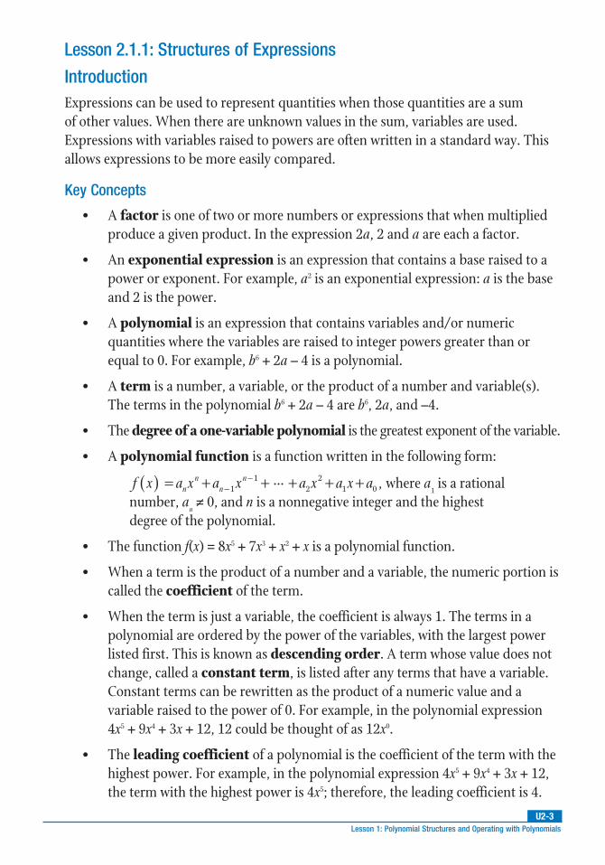
IntroductionExpressions can be used to represent quantities when those quantities are a sum of other values. When there are unknown values in the sum, variables are used. Expressions with variables raised to powers are often written in a standard way. This allows expressions to be more easily compared.
Key Concepts
• A factor is one of two or more numbers or expressions that when multiplied produce a given product. In the expression 2a, 2 and a are each a factor.
• An exponential expression is an expression that contains a base raised to a power or exponent. For example, a2 is an exponential expression: a is the base and 2 is the power.
• A polynomial is an expression that contains variables and/or numeric quantities where the variables are raised to integer powers greater than or equal to 0. For example, b6 + 2a – 4 is a polynomial.
• A term is a number, a variable, or the product of a number and variable(s). The terms in the polynomial b6 + 2a – 4 are b6, 2a, and –4.
• The degree of a one-variable polynomial is the greatest exponent of the variable.
• A polynomial function is a function written in the following form:
f x a x a x a x a x ann
nn ,1
12
21 0( ) = + + … + + +−
− ... f x a x a x a x a x ann
nn ,1
12
21 0( ) = + + … + + +−
− where a1 is a rational
number, an ≠ 0, and n is a nonnegative integer and the highest
degree of the polynomial.
• The function f(x) = 8x5 + 7x3 + x2 + x is a polynomial function.
• When a term is the product of a number and a variable, the numeric portion is called the coefficient of the term.
• When the term is just a variable, the coefficient is always 1. The terms in a polynomial are ordered by the power of the variables, with the largest power listed first. This is known as descending order. A term whose value does not change, called a constant term, is listed after any terms that have a variable. Constant terms can be rewritten as the product of a numeric value and a variable raised to the power of 0. For example, in the polynomial expression 4x5 + 9x4 + 3x + 12, 12 could be thought of as 12x0.
• The leading coefficient of a polynomial is the coefficient of the term with the highest power. For example, in the polynomial expression 4x5 + 9x4 + 3x + 12, the term with the highest power is 4x5; therefore, the leading coefficient is 4.
Lesson 2.1.1: Structures of Expressions
U2-4Unit 2: Polynomial Functions
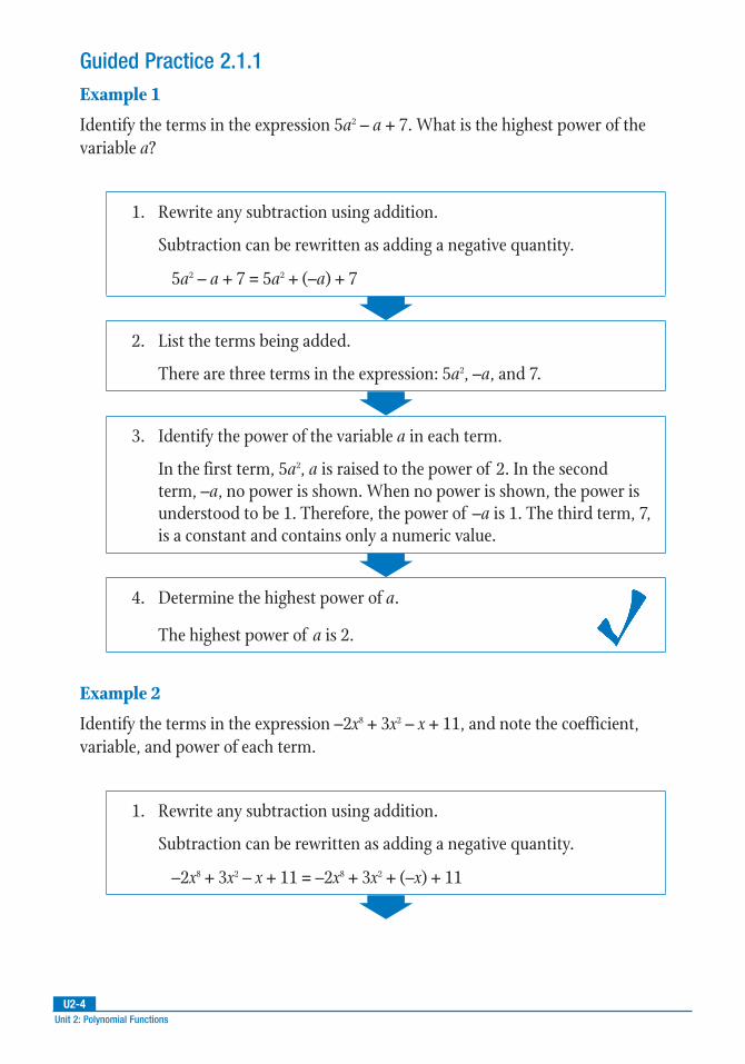
Example 2
Identify the terms in the expression –2x8 + 3x2 – x + 11, and note the coefficient, variable, and power of each term.
1. Rewrite any subtraction using addition.
Subtraction can be rewritten as adding a negative quantity.
–2x8 + 3x2 – x + 11 = –2x8 + 3x2 + (–x) + 11
Example 1
Identify the terms in the expression 5a2 – a + 7. What is the highest power of the variable a?
1. Rewrite any subtraction using addition.
Subtraction can be rewritten as adding a negative quantity.
5a2 – a + 7 = 5a2 + (–a) + 7
2. List the terms being added.
There are three terms in the expression: 5a2, –a, and 7.
3. Identify the power of the variable a in each term.
In the first term, 5a2, a is raised to the power of 2. In the second term, –a, no power is shown. When no power is shown, the power is understood to be 1. Therefore, the power of –a is 1. The third term, 7, is a constant and contains only a numeric value.
4. Determine the highest power of a.
The highest power of a is 2.
Guided Practice 2.1.1

U2-5Lesson 1: Polynomial Structures and Operating with Polynomials
2. List the terms being added.
There are four terms in the expression: –2x8, 3x2, –x, and 11.
3. Identify the coefficient, variable, and power of each term.
The coefficient is the number being multiplied by the variable. The variable is the quantity represented by a letter. The power is the value of the exponent of the variable.
The term –2x8 has a coefficient of –2, a variable of x, and a power of 8.
The term 3x2 has a coefficient of 3, a variable of x, and a power of 2.
The term –x has a coefficient of –1, a variable of x, and a power of 1.
The term 11 is a constant; it contains only a numeric value.
Example 3
Write a polynomial function in descending order that contains the terms –x, 10x5, 4x3, and x2. Determine the degree of the polynomial function.
1. Identify the power of the variable of each term.
The power of the variable is the value of the exponent of the variable.
When no power is shown, the power is 1. Therefore, the power of the term –x is 1.
The power of the term 10x5 is 5.
The power of the term 4x3 is 3.
The power of the term x2 is 2.
2. Order the terms in descending order using the powers of the exponents.
The term with the highest power is listed first, then the term with the next highest power, and so on, with a constant listed last.
10x5, 4x3, x2, –x

U2-6Unit 2: Polynomial Functions
3. Sum the terms to write the polynomial function of the given variable.
The variable in each term is x, so the function will be a function of x, written f(x). Write f(x) as the sum of the terms in descending order, with the term that has the highest power listed first.
f(x) = 10x5 + 4x3 + x2 + (–x)
f(x) = 10x5 + 4x3 + x2 – x
4. Determine the degree of the polynomial.
The degree of a polynomial is the highest power of the variable.
The term with the highest power is listed first in the function, 10x5, and x has a power of 5.
The degree of the polynomial function f(x) is 5.
UNIT 2 • POLYNOMIAL FUNCTIONSLesson 1: Polynomial Structures and Operating with Polynomials
PRACTICE
U2-7Lesson 1: Polynomial Structures and Operating with Polynomials
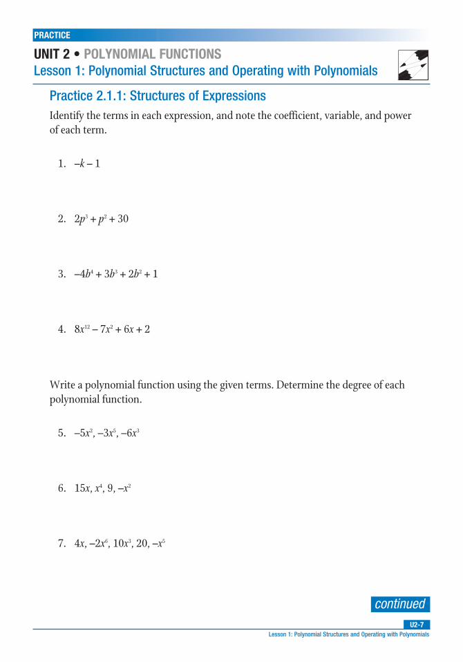
Identify the terms in each expression, and note the coefficient, variable, and power of each term.
1. –k – 1
2. 2p3 + p2 + 30
3. –4b4 + 3b3 + 2b2 + 1
4. 8x12 – 7x2 + 6x + 2
Write a polynomial function using the given terms. Determine the degree of each polynomial function.
5. –5x2, –3x5, –6x3
6. 15x, x4, 9, –x2
7. 4x, –2x6, 10x3, 20, –x5
continued
Practice 2.1.1: Structures of Expressions

UNIT 2 • POLYNOMIAL FUNCTIONSLesson 1: Polynomial Structures and Operating with Polynomials
PRACTICE
U2-8Unit 2: Polynomial Functions
Each of the figures below is divided into separate parts with each area written within that part. Find the total area of each figure. All units are in square inches.
8.
10x13
9.
30
5x2
14x
10.
50
25x2
12x
2x3
U2-9Lesson 1: Polynomial Structures and Operating with Polynomials
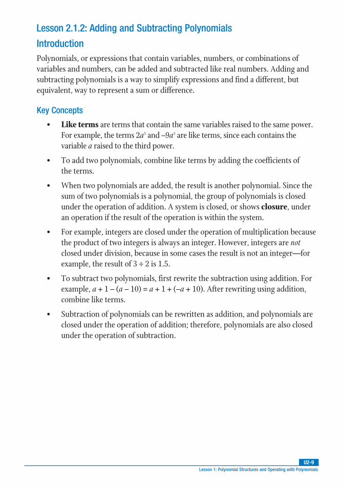
Lesson 2.1.2: Adding and Subtracting Polynomials
IntroductionPolynomials, or expressions that contain variables, numbers, or combinations of variables and numbers, can be added and subtracted like real numbers. Adding and subtracting polynomials is a way to simplify expressions and find a different, but equivalent, way to represent a sum or difference.
Key Concepts
• Like terms are terms that contain the same variables raised to the same power. For example, the terms 2a3 and –9a3 are like terms, since each contains the variable a raised to the third power.
• To add two polynomials, combine like terms by adding the coefficients of the terms.
• When two polynomials are added, the result is another polynomial. Since the sum of two polynomials is a polynomial, the group of polynomials is closed under the operation of addition. A system is closed, or shows closure, under an operation if the result of the operation is within the system.
• For example, integers are closed under the operation of multiplication because the product of two integers is always an integer. However, integers are not closed under division, because in some cases the result is not an integer—for example, the result of 3 ÷ 2 is 1.5.
• To subtract two polynomials, first rewrite the subtraction using addition. For example, a + 1 – (a – 10) = a + 1 + (–a + 10). After rewriting using addition, combine like terms.
• Subtraction of polynomials can be rewritten as addition, and polynomials are closed under the operation of addition; therefore, polynomials are also closed under the operation of subtraction.

U2-10Unit 2: Polynomial Functions
Example 1
Simplify (2x2 + x + 10) + (7x2 + 14).
1. Rewrite the sum so that any like terms are together.
The first polynomial, 2x2 + x + 10, has a term with a power of 2, a term with a power of 1, and a constant term. The second polynomial, 7x2 + 14, has a term with a power of 2 and a constant term. The terms with the same powers and variables are like terms, as are the constants.
(2x2 + x + 10) + (7x2 + 14)
= 2x2 + 7x2 + x + 10 + 14
2. Find the sum of any constants.
The previous expression contains two constants: 10 and 14.
2x2 + 7x2 + x + 10 + 14
= 2x2 + 7x2 + x + 24
3. Find the sum of any terms with the same variable raised to the same power by adding the coefficients of the terms.
2x2 + 7x2 + x + 24
= (2 + 7)x2 + x + 24
= 9x2 + x + 24
(2x2 + x + 10) + (7x2 + 14) is equivalent to 9x2 + x + 24.
Guided Practice 2.1.2

U2-11Lesson 1: Polynomial Structures and Operating with Polynomials
Example 2
Simplify (6x4 – x3 – 3x2 + 20) + (10x3 – 4x2 + 9).
1. Rewrite any subtraction using addition.
Subtraction can be rewritten as adding a negative.
(6x4 – x3 – 3x2 + 20) + (10x3 – 4x2 + 9)
= [6x4 + (–x3) + (–3x2) + 20] + [10x3 + (–4x2) + 9]
2. Rewrite the sum so that any like terms are together.
Be sure to keep any negatives with the terms.
[6x4 + (–x3) + (–3x2) + 20] + [10x3 + (–4x2) + 9]
= 6x4 + (–x3) + 10x3 + (–3x2) + (–4x2) + 20 + 9
3. Find the sum of any constants.
The previous expression contains two constants: 20 and 9.
6x4 + (–x3) + 10x3 + (–3x2) + (–4x2) + 20 + 9
= 6x4 + (–x3) + 10x3 + (–3x2) + (–4x2) + 29
4. Find the sum of any terms with the same variable raised to the same power.
The previous expression contains the following like terms: (–x3) and 10x3; (–3x2) and (–4x2).
Add the coefficients of any like terms, being sure to keep any negatives with the coefficients.
6x4 + (–x3) + 10x3 + (–3x2) + (–4x2) + 29
= 6x4 + (–1 + 10)x3 + [–3 + (–4)]x2 + 29
= 6x4 + 9x3 – 7x2 + 29
(6x4 – x3 – 3x2 + 20) + (10x3 – 4x2 + 9) is equivalent to 6x4 + 9x3 – 7x2 + 29.

U2-12Unit 2: Polynomial Functions
Example 3
Simplify (–x6 + 7x2 + 11) – (12x6 + 4x5 – 2x + 1).
1. Rewrite the difference as a sum.
A difference can be written as the sum of a negative quantity.
Distribute the negative in the second polynomial.
(–x6 + 7x2 + 11) – (12x6 + 4x5 – 2x + 1)
= (–x6 + 7x2 + 11) + [–(12x6 + 4x5 – 2x + 1)]
= (–x6 + 7x2 + 11) + (–12x6) + (–4x5) + 2x + (–1)
2. Rewrite the sum so that any like terms are together.
Be sure to keep any negatives with the coefficients.
(–x6 + 7x2 + 11) + (–12x6) + (–4x5) + 2x + (–1)
= –x6 + (–12x6) + (–4x5) + 7x2 + 2x + 11 + (–1)
3. Find the sum of any constants.
The previous expression contains two constants: 11 and (–1).
–x6 + (–12x6) + (–4x5) + 7x2 + 2x + 11 + (–1)
= –x6 + (–12x6) + (–4x5) + 7x2 + 2x + 10
4. Find the sum of any terms with the same variable raised to the same power.
The previous expression contains the following like terms: –x6 and (–12x6).
–x6 + (–12x6) + (–4x5) + 7x2 + 2x + 10
= [(–1) + (–12)]x6 + (–4x5) + 7x2 + 2x + 10
= –13x6 + (–4x5) + 7x2 + 2x + 10
= –13x6 – 4x5 + 7x2 + 2x + 10
(–x6 + 7x2 + 11) – (12x6 + 4x5 – 2x + 1) is equivalent to –13x6 – 4x5 + 7x2 + 2x + 10.
UNIT 2 • POLYNOMIAL FUNCTIONSLesson 1: Polynomial Structures and Operating with Polynomials
PRACTICE
U2-13Lesson 1: Polynomial Structures and Operating with Polynomials
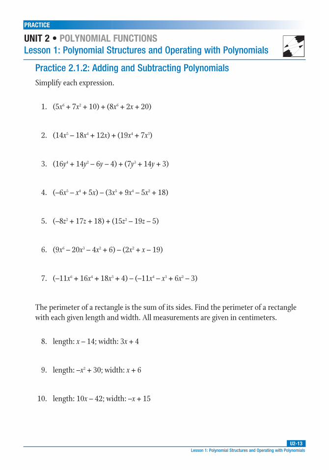
Simplify each expression.
1. (5x6 + 7x2 + 10) + (8x6 + 2x + 20)
2. (14x5 – 18x4 + 12x) + (19x4 + 7x3)
3. (16y4 + 14y2 – 6y – 4) + (7y3 + 14y + 3)
4. (–6x5 – x4 + 5x) – (3x5 + 9x4 – 5x2 + 18)
5. (–8z2 + 17z + 18) + (15z2 – 19z – 5)
6. (9x6 – 20x3 – 4x2 + 6) – (2x2 + x – 19)
7. (–11x6 + 16x4 + 18x3 + 4) – (–11x4 – x3 + 6x2 – 3)
The perimeter of a rectangle is the sum of its sides. Find the perimeter of a rectangle with each given length and width. All measurements are given in centimeters.
8. length: x – 14; width: 3x + 4
9. length: –x2 + 30; width: x + 6
10. length: 10x – 42; width: –x + 15
Practice 2.1.2: Adding and Subtracting Polynomials

U2-14Unit 2: Polynomial Functions
Lesson 2.1.3: Multiplying Polynomials
IntroductionTo simplify an expression, such as (a + bx)(c + dx), polynomials can be multiplied. Unlike addition and subtraction of polynomial terms, any two terms can be multiplied, even if the variables or powers are different. Using properties of exponents and combining like terms can allow you to simplify products of polynomials.
Key Concepts
• To multiply two polynomials, multiply each term in the first polynomial by each term in the second polynomial.
• The Distributive Property can be used to simplify the product of two polynomials, each with two terms: (a + b) • (c + d) = (a + b) • c + (a + b) • d = ac + bc + ad + bd.
• To find the product of two variables raised to a power, use the properties of exponents: x n • x m = x n + m; x n • ym = x nym.
• To find the product of a variable with a coefficient and a numeric quantity, multiply the coefficient by the numeric quantity; for real numbers a and b, ax • b = abx.
• After multiplying all terms, simplify the expression by combining like terms.
• The product of two polynomials is a polynomial, so the system of polynomials is closed under multiplication.

U2-15Lesson 1: Polynomial Structures and Operating with Polynomials
Example 1
Simplify the expression (x2 + 3)(x + 6).
1. Rewrite the product using the Distributive Property.
Multiply each term in the first polynomial by each term in the second polynomial.
(x2 + 3)(x + 6) = (x2 • x) + (3 • x) + (x2 • 6) + (3 • 6)
2. Use properties of exponents to simplify the expression.
x is x raised to the first power, or x1.
(x2 • x) + (3 • x) + (x2 • 6) + (3 • 6) Distributed expression
= (x2 • x1) + (3 • x) + (x2 • 6) + (3 • 6) Substitute x1 for x when multiplying terms that both have variables.
= (x2 + 1) + (3 • x) + (x2 • 6) + (3 • 6) Since x n • xm = x n + m, add the exponents.
= x3 + (3 • x) + (x2 • 6) + (3 • 6) Simplify.
3. Simplify any remaining products.
The product of a number and a variable is written with the number first, as the coefficient of the variable.
x3 + (3 • x) + (x2 • 6) + (3 • 6) Expression from the previous step
= x3 + 3x + 6x2 + 18 Simplify.
= x3 + 6x2 + 3x + 18 Rewrite in descending order.
The expression (x2 + 3)(x + 6) is equivalent to x3 + 6x2 + 3x + 18.
Guided Practice 2.1.3
U2-16Unit 2: Polynomial Functions
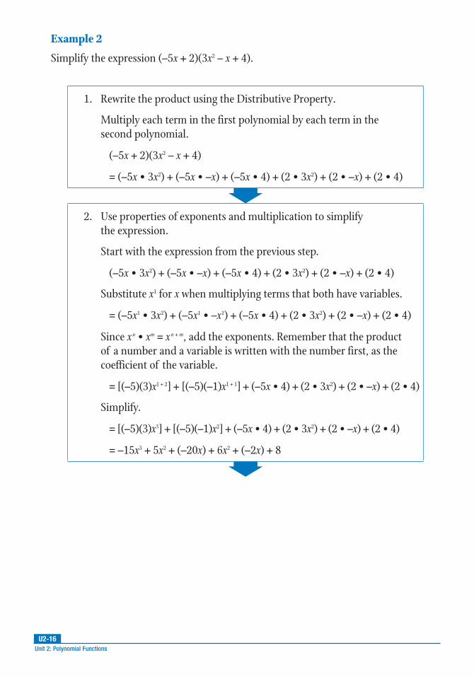
Example 2
Simplify the expression (–5x + 2)(3x2 – x + 4).
1. Rewrite the product using the Distributive Property.
Multiply each term in the first polynomial by each term in the second polynomial.
(–5x + 2)(3x2 – x + 4)
= (–5x • 3x2) + (–5x • –x) + (–5x • 4) + (2 • 3x2) + (2 • –x) + (2 • 4)
2. Use properties of exponents and multiplication to simplify the expression.
Start with the expression from the previous step.
(–5x • 3x2) + (–5x • –x) + (–5x • 4) + (2 • 3x2) + (2 • –x) + (2 • 4)
Substitute x1 for x when multiplying terms that both have variables.
= (–5x1 • 3x2) + (–5x1 • –x1) + (–5x • 4) + (2 • 3x2) + (2 • –x) + (2 • 4)
Since x n • xm = x n + m, add the exponents. Remember that the product of a number and a variable is written with the number first, as the coefficient of the variable.
= [(–5)(3)x1 + 2] + [(–5)(–1)x1 + 1] + (–5x • 4) + (2 • 3x2) + (2 • –x) + (2 • 4)
Simplify.
= [(–5)(3)x3] + [(–5)(–1)x2] + (–5x • 4) + (2 • 3x2) + (2 • –x) + (2 • 4)
= –15x3 + 5x2 + (–20x) + 6x2 + (–2x) + 8
U2-17Lesson 1: Polynomial Structures and Operating with Polynomials
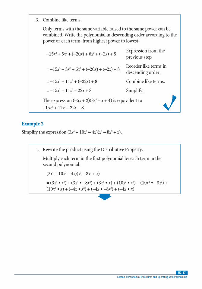
3. Combine like terms.
Only terms with the same variable raised to the same power can be combined. Write the polynomial in descending order according to the power of each term, from highest power to lowest.
–15x3 + 5x2 + (–20x) + 6x2 + (–2x) + 8Expression from the previous step
= –15x3 + 5x2 + 6x2 + (–20x) + (–2x) + 8Reorder like terms in descending order.
= –15x3 + 11x2 + (–22x) + 8 Combine like terms.
= –15x3 + 11x2 – 22x + 8 Simplify.
The expression (–5x + 2)(3x2 – x + 4) is equivalent to –15x3 + 11x2 – 22x + 8.
Example 3
Simplify the expression (3x4 + 10x2 – 4x)(x3 – 8x2 + x).
1. Rewrite the product using the Distributive Property.
Multiply each term in the first polynomial by each term in the second polynomial.
(3x4 + 10x2 – 4x)(x3 – 8x2 + x)
= (3x4 • x3) + (3x4 • –8x2) + (3x4 • x) + (10x2 • x3) + (10x2 • –8x2) + (10x2 • x) + (–4x • x3) + (–4x • –8x2) + (–4x • x)

U2-18Unit 2: Polynomial Functions
2. Use properties of exponents and multiplication to simplify any expressions.
Start with the expression from the previous step.
(3x4 • x3) + (3x4 • –8x2) + (3x4 • x) + (10x2 • x3) + (10x2 • –8x2) + (10x2 • x) + (–4x • x3) + (–4x • –8x2) + (–4x • x)
Substitute x1 for x when multiplying terms that both have variables.
= (3x4 • x3) + (3x4 • –8x2) + [3x4 • (x1)] + (10x2 • x3) + (10x2 • –8x2) + [10x2 • (x1)] + [–4(x1) • x3] + [–4(x1) • –8x2] + [–4(x1) • (x1)]
Since x n • xm = x n + m, add the exponents. Remember that the product of a number and a variable is written with the number first, as the coefficient of the variable.
= [(3)(1)x 4 + 3] + [(3)(–8)x 4 + 2] + [(3)(1)x 4 + 1] + [(10)(1)x2 + 3] + [(10)(–8)x2 + 2] + [(10)(1)x2 + 1] + [(–4)(1)x1 + 3] + [(–4)(–8)x1 + 2] + [(–4)(1)x1 + 1]
Simplify.
= [(3)(1)x7] + [(3)(–8)x6] + [(3)(1)x5] + [(10)(1)x5] + [(10)(–8)x4] + [(10)(1)x3] + [(–4)(1)x4] + [(–4)(–8)x3] + [(–4)(1)x2]
= 3x7 + (–24x6) + 3x5 + 10x5 + (–80x4) + 10x3 + (–4x4) + 32x3 + (–4x2)
3. Combine like terms.
Only terms with the same variable raised to the same power can be combined.
Write the polynomial in descending order according to the power of each term with a variable, from highest power to lowest.
3x7 + (–24x6) + 3x5 + 10x5 + (–80x4) + 10x3 + (–4x4) + 32x3 + (–4x2)
Expression from the previous step
= 3x7 + (–24x6) + 3x5 + 10x5 + (–80x4) + (–4x4) + 10x3 + 32x3 + (–4x2)
Reorder like terms in descending order.
= 3x7 + (–24x6) + 13x5 + (–84x4) + 42x3 + (–4x2)
Combine like terms.
= 3x7 – 24x6 + 13x5 – 84x4 + 42x3 – 4x2 Simplify.
The expression (3x4 + 10x2 – 4x)(x3 – 8x2 + x) is equivalent to 3x7 – 24x6 + 13x5 – 84x4 + 42x3 – 4x2.

UNIT 2 • POLYNOMIAL FUNCTIONSLesson 1: Polynomial Structures and Operating with Polynomials
PRACTICE
U2-19Lesson 1: Polynomial Structures and Operating with Polynomials
Simplify each expression.
1. (5x2 – 2)(x3 + 4)
2. (3y4 + y2)(–y3 + 10)
3. (–6z3 – 3z + 1)(4z2 – 2z)
4. (–x4 + 5x3)(7x2 – 2x + 8)
5. (y5 – 4y2 + 3)(y5 – 1)
6. (2x3 + x + 1)(3x2 – 6x + 5)
7. (–8x3 + 3x2 + 4)(–x4 – x – 6)
The area of a rectangle is found using the formula length • width. Find the area of a rectangle with the given length and width. All measurements are given in meters.
8. length: x + 14; width: x – 4
9. length: 4x – 2; width: x2 + 1
10. length: 8x + 7; width: 3x2 – 10
Practice 2.1.3: Multiplying Polynomials

Unit 2: Polynomial FunctionsU2-20
Lesson 2: Proving IdentitiesUNIT 2 • POLYNOMIAL FUNCTIONS
Common Core Georgia Performance Standards
MCC9–12.N.CN.8 (+)
MCC9–12.A.SSE.1a★
MCC9–12.A.SSE.1b★
MCC9–12.A.SSE.2
MCC9–12.A.APR.4
MCC9–12.A.APR.5 (+)
Essential Questions
1. How do polynomial identities help when expanding or factoring polynomials?
2. How can multiplication of binomials be used to find products of complex numbers?
3. What patterns are used to find powers of binomials?
WORDS TO KNOW
Binomial Theorem a theorem stating that a binomial (a + b)n
can be expanded using the formula
∑( )−• = + • +
−•
• +− −• •
• + +−
=
− − −n
n k ka b a b
na b
n na b
n n na b a bn k k
k
nn n n n n
!
! !1
1
( 1)
1 2
( 1)( 2)
1 2 31
0
0 1 1 2 2 3 3 0
∑( )−• = + • +
−•
• +− −• •
• + +−
=
− − −n
n k ka b a b
na b
n na b
n n na b a bn k k
k
nn n n n n
!
! !1
1
( 1)
1 2
( 1)( 2)
1 2 31
0
0 1 1 2 2 3 3 0
complex conjugate the complex number that when multiplied by another complex number produces a value that is wholly real; the complex conjugate of a + bi is a – bi
complex number a number of the form a + bi, where a and b are real numbers and i is the imaginary unit
factorial the product of an integer and all preceding positive integers, represented using a ! symbol; n! = n • (n – 1) • (n – 2) • … • 1. For example, 5! = 5 • 4 • 3 • 2 • 1. By definition, 0! = 1.
U2-21Lesson 2: Proving Identities
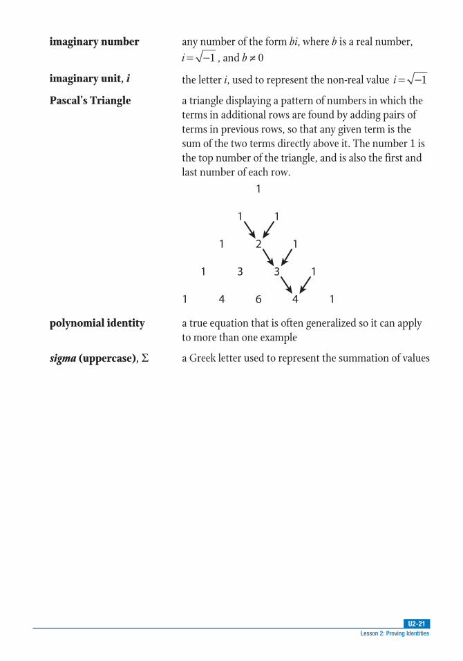
imaginary number any number of the form bi, where b is a real number, 1= −i , and b ≠ 0
imaginary unit, i the letter i, used to represent the non-real value 1= −i
Pascal’s Triangle a triangle displaying a pattern of numbers in which the terms in additional rows are found by adding pairs of terms in previous rows, so that any given term is the sum of the two terms directly above it. The number 1 is the top number of the triangle, and is also the first and last number of each row.
1
1
1
1
1
1
21
331
4641
polynomial identity a true equation that is often generalized so it can apply to more than one example
sigma (uppercase), Σ a Greek letter used to represent the summation of values

U2-22Unit 2: Polynomial Functions
Recommended Resources• Interactive Mathematics. “The Binomial Theorem.”
http://www.walch.com/rr/00161
This site includes a review of binomials, several examples showing binomial expansion, and a summary of Pascal’s Triangle. Users can enter values into the interactive applets to find factorials of positive integers up to 30, and expand binomials up to powers of 6.
• MathIsFun.com. “Binomial Theorem.”
http://www.walch.com/rr/00162
This site offers a simple yet effective review of binomials that leads into an explanation of the Binomial Theorem for (a + b)n. The review covers exponents, polynomials, and Pascal’s Triangle. Links are provided to sample questions that generate immediate feedback, along with explanations of answers.
• MathIsFun.com. “Factoring in Algebra.”
http://www.walch.com/rr/00163
This resource offers instruction on factoring polynomials, including how to apply polynomial identities to factors. The site also includes links to 10 multiple-choice practice questions, with immediate feedback and explanations.
• Virtual Nerd. “What’s the Formula for the Square of a Sum?”
http://www.walch.com/rr/00164
This brief video tutorial illuminates each step in deriving the formula for the square of a sum.
U2-23Lesson 2: Proving Identities
Lesson 2.2.1: Polynomial Identities
IntroductionPolynomials are often added, subtracted, and even multiplied. Doing so results in certain sums, differences, or products of polynomials appearing more commonly. Becoming familiar with certain polynomial identities can make the processes of expanding and factoring polynomials easier.
Key Concepts
• Identities can be used to expand or factor polynomial expressions.
• A polynomial identity is a true equation that is often generalized so it can apply to more than one example.
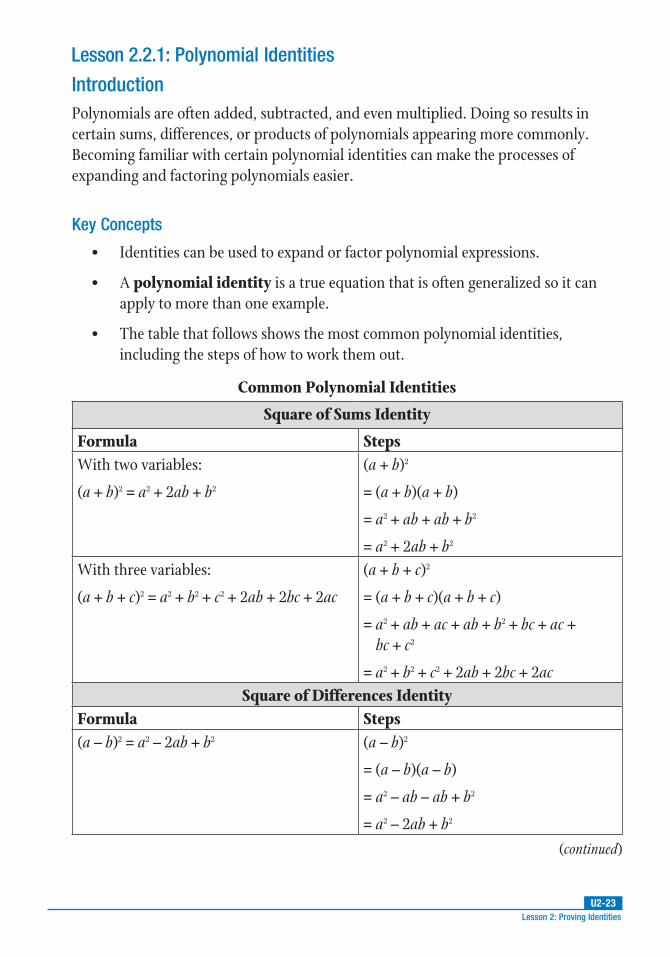
• The table that follows shows the most common polynomial identities, including the steps of how to work them out.
Common Polynomial Identities
Square of Sums Identity
Formula StepsWith two variables:
(a + b)2 = a2 + 2ab + b2
(a + b)2
= (a + b)(a + b)
= a2 + ab + ab + b2
= a2 + 2ab + b2
With three variables:
(a + b + c)2 = a2 + b2 + c2 + 2ab + 2bc + 2ac
(a + b + c)2
= (a + b + c)(a + b + c)
= a2 + ab + ac + ab + b2 + bc + ac + bc + c2
= a2 + b2 + c2 + 2ab + 2bc + 2acSquare of Differences Identity
Formula Steps(a – b)2 = a2 – 2ab + b2 (a – b)2
= (a – b)(a – b)
= a2 – ab – ab + b2
= a2 – 2ab + b2
(continued)
U2-24Unit 2: Polynomial Functions
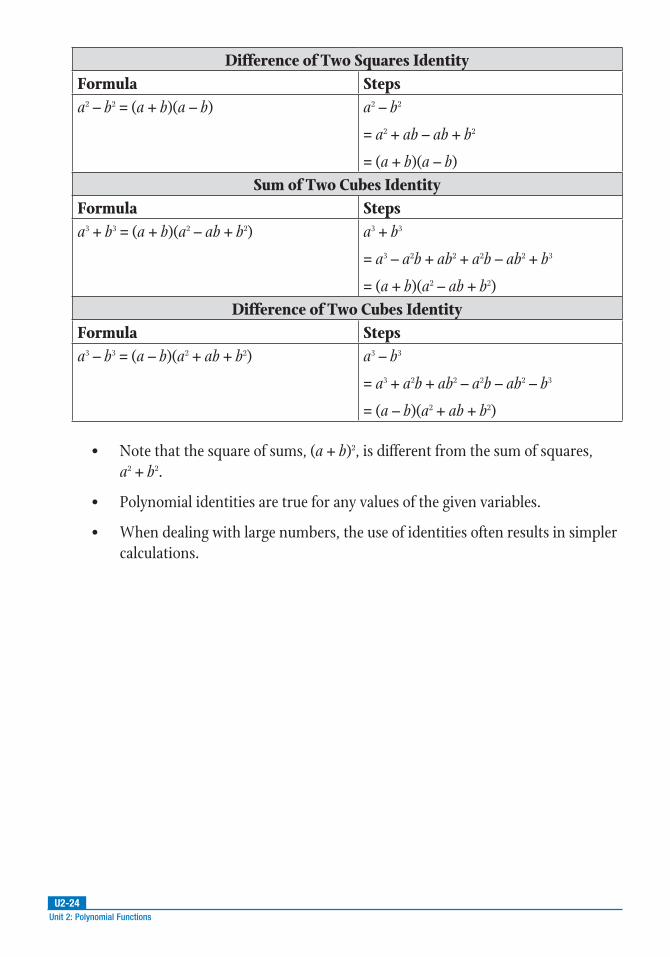
Difference of Two Squares IdentityFormula Stepsa2 – b2 = (a + b)(a – b) a2 – b2
= a2 + ab – ab + b2
= (a + b)(a – b)Sum of Two Cubes Identity
Formula Stepsa3 + b3 = (a + b)(a2 – ab + b2) a3 + b3
= a3 – a2b + ab2 + a2b – ab2 + b3
= (a + b)(a2 – ab + b2)Difference of Two Cubes Identity
Formula Stepsa3 – b3 = (a – b)(a2 + ab + b2) a3 – b3
= a3 + a2b + ab2 – a2b – ab2 – b3
= (a – b)(a2 + ab + b2)
• Note that the square of sums, (a + b)2, is different from the sum of squares, a2 + b2.
• Polynomial identities are true for any values of the given variables.
• When dealing with large numbers, the use of identities often results in simpler calculations.

U2-25Lesson 2: Proving Identities
Guided Practice 2.2.1Example 1
Use a polynomial identity to expand the expression (x – 14)2.
1. Determine which identity is written in the same form as the given expression.
The expression (x – 14)2 is written in the same form as the left side of the Square of Differences Identity: (a – b)2 = a2 – 2ab + b2.
Therefore, we can substitute the values from the expression (x – 14)2 into the Square of Differences Identity.
2. Replace a and b in the identity with the terms in the given expression.
For the given expression (x – 14)2, let x = a and 14 = b in the Square of Differences Identity.
(x – 14)2 Original expression
(a – b)2 = a2 – 2ab + b2 Square of Differences Identity
[(x) – (14)]2 = (x)2 – 2(x)(14) + (14)2 Substitute x for a and 14 for b in the Square of Differences Identity.
The rewritten identity is (x – 14)2 = x2 – 2(x)(14) + 142.
3. Simplify the expression by finding any products and evaluating any exponents.
The first term, x2, cannot be simplified further, but the other terms can.
(x – 14)2 = x2 – 2(x)(14) + 142 Equation from the previous step
= x2 – 28x + 142 Simplify 2(x)(14).
= x2 – 28x + 196 Square 14.
When expanded, the expression (x – 14)2 can be written as x2 – 28x + 196.
U2-26Unit 2: Polynomial Functions
Example 2
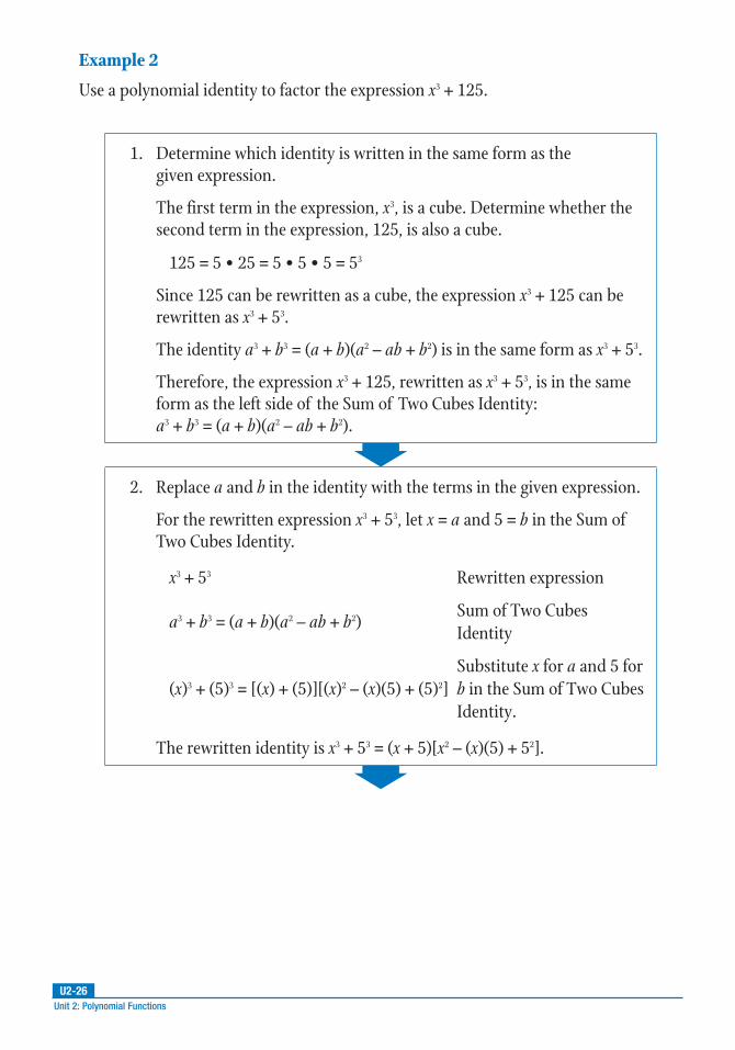
Use a polynomial identity to factor the expression x3 + 125.
1. Determine which identity is written in the same form as the given expression.
The first term in the expression, x3, is a cube. Determine whether the second term in the expression, 125, is also a cube.
125 = 5 • 25 = 5 • 5 • 5 = 53
Since 125 can be rewritten as a cube, the expression x3 + 125 can be rewritten as x3 + 53.
The identity a3 + b3 = (a + b)(a2 – ab + b2) is in the same form as x3 + 53.
Therefore, the expression x3 + 125, rewritten as x3 + 53, is in the same form as the left side of the Sum of Two Cubes Identity: a3 + b3 = (a + b)(a2 – ab + b2).
2. Replace a and b in the identity with the terms in the given expression.
For the rewritten expression x3 + 53, let x = a and 5 = b in the Sum of Two Cubes Identity.
x3 + 53 Rewritten expression
a3 + b3 = (a + b)(a2 – ab + b2) Sum of Two Cubes Identity
(x)3 + (5)3 = [(x) + (5)][(x)2 – (x)(5) + (5)2]Substitute x for a and 5 for b in the Sum of Two Cubes Identity.
The rewritten identity is x3 + 53 = (x + 5)[x2 – (x)(5) + 52].
U2-27Lesson 2: Proving Identities
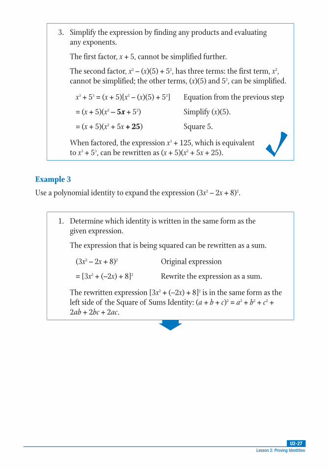
3. Simplify the expression by finding any products and evaluating any exponents.
The first factor, x + 5, cannot be simplified further.
The second factor, x2 – (x)(5) + 52, has three terms: the first term, x2, cannot be simplified; the other terms, (x)(5) and 52, can be simplified.
x3 + 53 = (x + 5)[x2 – (x)(5) + 52] Equation from the previous step
= (x + 5)(x2 – 5x + 52) Simplify (x)(5).
= (x + 5)(x2 + 5x + 25) Square 5.
When factored, the expression x3 + 125, which is equivalent to x3 + 53, can be rewritten as (x + 5)(x2 + 5x + 25).
Example 3
Use a polynomial identity to expand the expression (3x2 – 2x + 8)2.
1. Determine which identity is written in the same form as the given expression.
The expression that is being squared can be rewritten as a sum.
(3x2 – 2x + 8)2 Original expression
= [3x2 + (–2x) + 8]2 Rewrite the expression as a sum.
The rewritten expression [3x2 + (–2x) + 8]2 is in the same form as the left side of the Square of Sums Identity: (a + b + c)2 = a2 + b2 + c2 + 2ab + 2bc + 2ac.

U2-28Unit 2: Polynomial Functions
2. Replace a and b in the identity with the terms in the given expression.
For the expression [3x2 + (–2x) + 8]2, let 3x2 = a, –2x = b, and 8 = c in the Square of Sums Identity.
[3x2 + (–2x) + 8]2 Rewritten expression
(a + b + c)2 = a2 + b2 + c2 + 2ab + 2bc + 2ac Square of Sums Identity
[(3x2) + (–2x) + (8)]2 = (3x2)2 + (–2x)2 + (8)2 + 2(3x2)(–2x) + 2(–2x)(8) + 2(3x2)(8)
Substitute 3x2 for a, –2x for b, and 8 for c in the Square of Sums Identity.
The rewritten identity is [3x2 + (–2x) + 8]2 = (3x2)2 + (–2x)2 + 82 + 2(3x2)(–2x) + 2(–2x)(8) + 2(3x2)(8).
3. Simplify each term in the expression by finding any products and evaluating any exponents.
[3x2 + (–2x) + 8]2 = (3x2)2 + (–2x)2 + 82 + 2(3x2)(–2x) + 2(–2x)(8) + 2(3x2)(8)
Equation from the previous step
= 9x4 + (–2x)2 + 82 + 2(3x2)(–2x) + 2(–2x)(8) + 2(3x2)(8)
Simplify (3x2)2.
= 9x4 + 4x2 + 82 + 2(3x2)(–2x) + 2(–2x)(8) + 2(3x2)(8)
Simplify (–2x)2.
= 9x4 + 4x2 + 64 + 2(3x2)(–2x) + 2(–2x)(8) + 2(3x2)(8)
Square 8.
= 9x4 + 4x2 + 64 – 12x3 + 2(–2x)(8) + 2(3x2)(8)
Simplify 2(3x2)(–2x).
= 9x4 + 4x2 + 64 – 12x3 – 32x + 2(3x2)(8) Multiply 2(–2x)(8).
= 9x4 + 4x2 + 64 – 12x3 – 32x + 48x2 Multiply 2(3x2)(8).
U2-29Lesson 2: Proving Identities
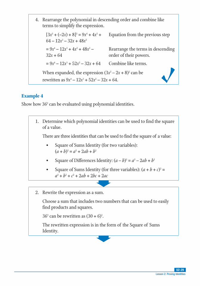
4. Rearrange the polynomial in descending order and combine like terms to simplify the expression.
[3x2 + (–2x) + 8]2 = 9x4 + 4x2 + 64 – 12x3 – 32x + 48x2
Equation from the previous step
= 9x4 – 12x3 + 4x2 + 48x2 – 32x + 64
Rearrange the terms in descending order of their powers.
= 9x4 – 12x3 + 52x2 – 32x + 64 Combine like terms.
When expanded, the expression (3x2 – 2x + 8)2 can be rewritten as 9x4 – 12x3 + 52x2 – 32x + 64.
Example 4
Show how 362 can be evaluated using polynomial identities.
1. Determine which polynomial identities can be used to find the square of a value.
There are three identities that can be used to find the square of a value:
• Square of Sums Identity (for two variables): (a + b)2 = a2 + 2ab + b2
• Square of Differences Identity: (a – b)2 = a2 – 2ab + b2
• Square of Sums Identity (for three variables): (a + b + c)2 = a2 + b2 + c2 + 2ab + 2bc + 2ac
2. Rewrite the expression as a sum.
Choose a sum that includes two numbers that can be used to easily find products and squares.
362 can be rewritten as (30 + 6)2.
The rewritten expression is in the form of the Square of Sums Identity.

U2-30Unit 2: Polynomial Functions
3. Use the sum and a polynomial identity to rewrite the expression.
For the expression (30 + 6)2, let 30 = a and 6 = b in the Square of Sums Identity.
(30 + 6)2 Rewritten expression
(a + b)2 = a2 + 2ab + b2 Square of Sums Identity
[(30) + (6)]2 = (30)2 + 2(30)(6) + (6)2 Substitute 30 for a and 6 for b in the Square of Sums Identity.
(30 + 6)2 = 900 + 360 + 36 Simplify each term.
(30 + 6)2 = 1296 Sum the terms.
The expression 362 is equal to 1,296.
UNIT 2 • POLYNOMIAL FUNCTIONSLesson 2: Proving Identities
PRACTICE
U2-31Lesson 2: Proving Identities
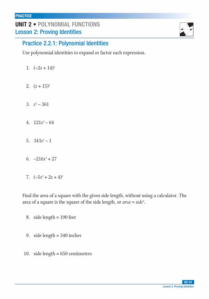
Use polynomial identities to expand or factor each expression.
1. (–2x + 14)2
2. (x + 15)2
3. x2 – 361
4. 121x2 – 64
5. 343x3 – 1
6. –216x3 + 27
7. (–5x2 + 2x + 4)2
Find the area of a square with the given side length, without using a calculator. The area of a square is the square of the side length, or area = side2.
8. side length = 190 feet
9. side length = 340 inches
10. side length = 650 centimeters
Practice 2.2.1: Polynomial Identities

U2-32Unit 2: Polynomial Functions
Lesson 2.2.2: Complex Polynomial Identities
IntroductionPolynomial identities can be used to find the product of complex numbers. A complex number is a number of the form a + bi, where a and b are real numbers and i is the imaginary unit. An expression that cannot be written using an identity with real numbers can be factored using the imaginary unit i.
Key Concepts
• An imaginary number is any number of the form bi, where b is a real number, 1= −i , and b ≠ 0. The imaginary unit i is used to represent the non-real
value 1= −i .
• Recall that i2 = –1.
• Polynomial identities and properties of the imaginary unit i can be used to expand or factor expressions with complex numbers.
• Complex conjugates are two complex numbers of the form a + bi and a – bi. Both numbers contain an imaginary part, but multiplying them produces a value that is wholly real. Therefore, the complex conjugate of a + bi is a – bi, and vice versa.
• The sum of two squares can be rewritten as the product of complex conjugates: a2 + b2 = (a + bi)(a – bi), where a and b are real numbers and i is the imaginary unit.
• Rewriting the sum of two squares in this way can allow you to either factor the sum of two squares or to find the product of complex conjugates.
• To prove this, find the product of the conjugates and simplify the expression.
(a + bi)(a – bi) = a • a + a • bi + a(–bi) + bi(–bi) = a2 + abi – abi – b2i2 = a2 – b2(–1) = a2 + b2
• This factored form of the sum of two squares can also include variables, such as a2x2 + b2 = (ax + bi)(ax – bi), where x is a variable, a and b are real numbers, and i is the imaginary unit.
U2-33Lesson 2: Proving Identities
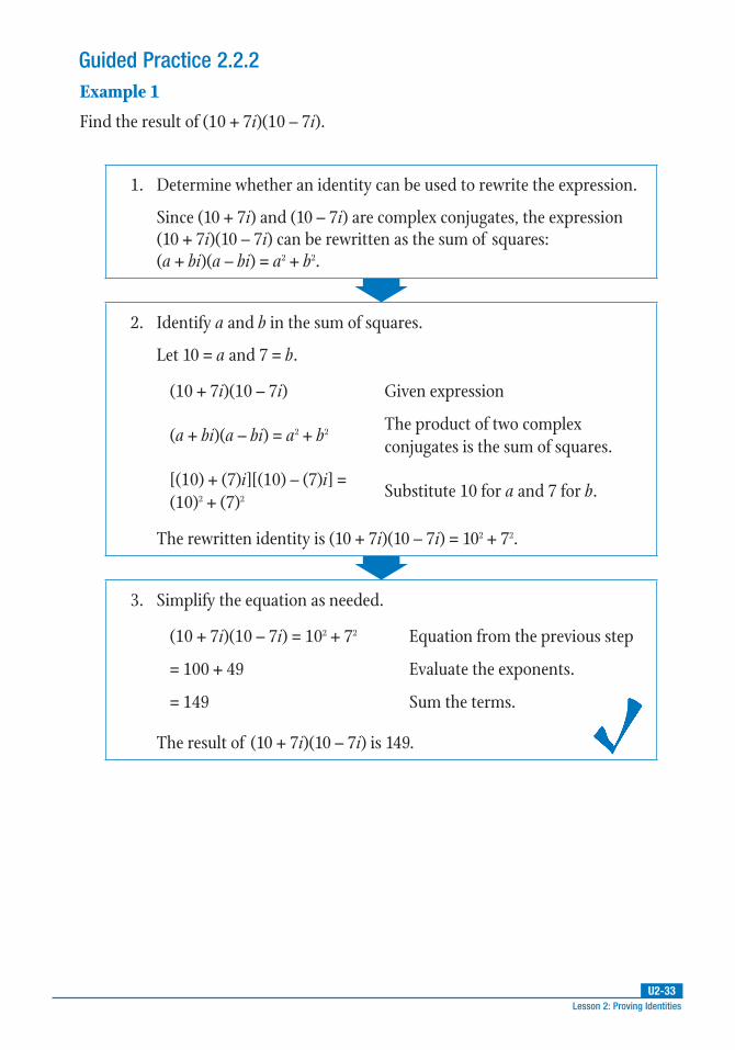
Guided Practice 2.2.2Example 1
Find the result of (10 + 7i)(10 – 7i).
1. Determine whether an identity can be used to rewrite the expression.
Since (10 + 7i) and (10 – 7i) are complex conjugates, the expression (10 + 7i)(10 – 7i) can be rewritten as the sum of squares: (a + bi)(a – bi) = a2 + b2.
2. Identify a and b in the sum of squares.
Let 10 = a and 7 = b.
(10 + 7i)(10 – 7i) Given expression
(a + bi)(a – bi) = a2 + b2 The product of two complex conjugates is the sum of squares.
[(10) + (7)i][(10) – (7)i] = (10)2 + (7)2 Substitute 10 for a and 7 for b.
The rewritten identity is (10 + 7i)(10 – 7i) = 102 + 72.
3. Simplify the equation as needed.
(10 + 7i)(10 – 7i) = 102 + 72 Equation from the previous step
= 100 + 49 Evaluate the exponents.
= 149 Sum the terms.
The result of (10 + 7i)(10 – 7i) is 149.

U2-34Unit 2: Polynomial Functions
Example 2
Factor the expression 9x2 + 169.
1. Determine whether an identity can be used to rewrite the expression.
Both 9 and 169 are perfect squares; therefore, 9x2 + 169 is a sum of squares.
The original expression can be rewritten using exponents.
9x2 + 169 Original expression
= (3x)2 + (13)2 Rewrite each term using exponents.
= 32x2 + 132 Rewrite (3x)2 as the product of two squares.
2. Identify a and b in the sum of squares.
The expression 32x2 + 132 is in the form a2x2 + b2, which can be rewritten using the factored form of the sum of squares: a2x2 + b2 = (ax + bi)(ax – bi).
In the rewritten expression 32x2 + 132, let 3 = a and 13 = b.
3. Factor the sum of squares.
a2x2 + b2 = (ax + bi)(ax – bi)The sum of squares is the product of complex conjugates.
(3)2x2 + (13)2 = [(3)x + (13)i][(3)x – (13)i]Substitute 3 for a and 13 for b.
9x2 + 169 = (3x + 13i)(3x – 13i) Evaluate the exponents.
When factored, the expression 9x2 + 169 is written as (3x + 13i)(3x – 13i).

U2-35Lesson 2: Proving Identities
Example 3
Find the result of (8x + 15i)(8x – 15i).
1. Determine whether an identity can be used to rewrite the expression.
Since (8x + 15i) and (8x – 15i) are complex conjugates, the expression can be rewritten as the sum of squares: (ax + bi)(ax – bi) = a2x2 + b2.
2. Identify a and b in the sum of squares.
Let 8 = a and 15 = b in the expression.
3. Use the factored form to determine the sum of squares.
(8x + 15i)(8x – 15i) Original expression
(ax + bi)(ax – bi) = a2x2 + b2 The product of complex conjugates is the sum of squares.
[(8)x + (15)i][(8)x – (15)i] = (8)2x2 + (15)2
Substitute 8 for a and 15 for b.
(8x + 15i)(8x – 15i) = 64x2 + 225 Evaluate the exponents.
The result of (8x + 15i)(8x – 15i) is 64x2 + 225.
UNIT 2 • POLYNOMIAL FUNCTIONSLesson 2: Proving Identities
PRACTICE
U2-36Unit 2: Polynomial Functions
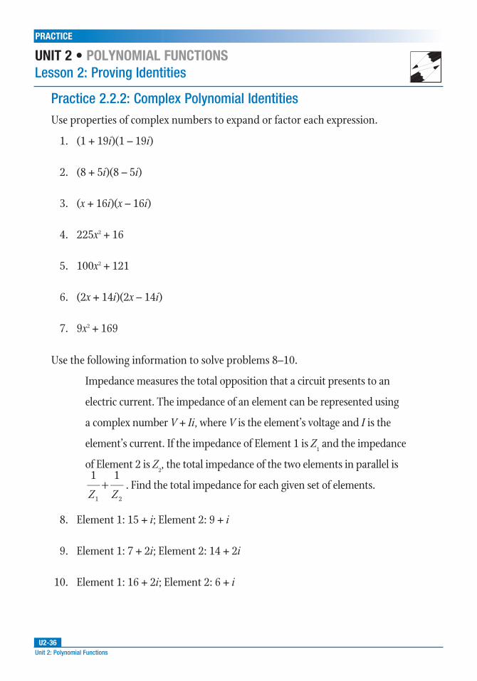
Use properties of complex numbers to expand or factor each expression.
1. (1 + 19i)(1 – 19i)
2. (8 + 5i)(8 – 5i)
3. (x + 16i)(x – 16i)
4. 225x2 + 16
5. 100x2 + 121
6. (2x + 14i)(2x – 14i)
7. 9x2 + 169
Use the following information to solve problems 8–10.
Impedance measures the total opposition that a circuit presents to an
electric current. The impedance of an element can be represented using
a complex number V + Ii, where V is the element’s voltage and I is the
element’s current. If the impedance of Element 1 is Z1 and the impedance
of Element 2 is Z2, the total impedance of the two elements in parallel is
1 1
1 2
+Z Z
. Find the total impedance for each given set of elements.
8. Element 1: 15 + i; Element 2: 9 + i
9. Element 1: 7 + 2i; Element 2: 14 + 2i
10. Element 1: 16 + 2i; Element 2: 6 + i
Practice 2.2.2: Complex Polynomial Identities

U2-37
Lesson 2.2.3:
Lesson 2: Proving Identities
IntroductionExpanding binomial expressions can sometimes be tedious and time-consuming, but the expansion of binomials raised to a power follows patterns. Understanding these patterns not only helps with determining the binomial expansion, but also with finding single terms in a binomial.
Key Concepts
• When a binomial is raised to a power, (a + b)n, there is a pattern in both the powers of the terms and the coefficients of the terms; a and b can be numbers, variables, or a combination of numbers and variables.
• The powers of the terms of the expanded form of (a + b)n follow the pattern anb0, an – 1b1, an – 2b2, … , a2bn – 2, a1bn – 1, a0bn.
• The power of a is n – k, where k is the term number. Note that the first term is term number 0, or k = 0. The power of b is k.
• For example, if n = 1, (a + b)1, the powers of the terms are a1 and b1. If n = 2, (a + b)2, the powers of the terms are a2, a1b1, and b2. If n = 3, (a + b)3, the powers of the terms are a3, a2b1, a1b2, and b3.
• Pascal’s Triangle is a triangle displaying a pattern of numbers in which the terms in additional rows are found by adding pairs of terms in the previous rows, so that any given term is the sum of the two terms directly above it.
1Row 0
Row 1
Row 2
Row 3
Row 4
1
1
1
1
1
21
331
4641
The sum of two terms is directly below them.
• Notice that the number 1 is the top number of the triangle, and is also the first and last number of each row.
Lesson 2.2.3: The Binomial Theorem
U2-38Unit 2: Polynomial Functions
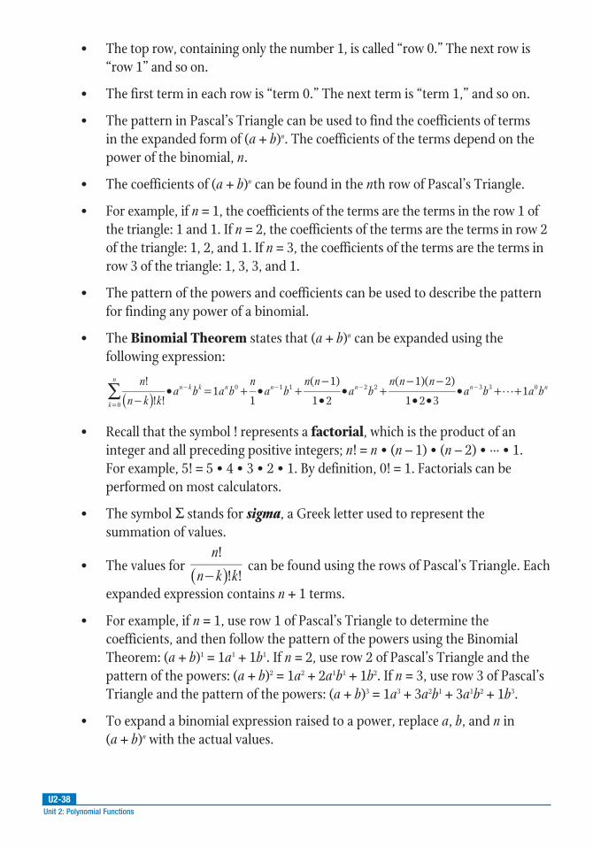
• The top row, containing only the number 1, is called “row 0.” The next row is “row 1” and so on.
• The first term in each row is “term 0.” The next term is “term 1,” and so on.
• The pattern in Pascal’s Triangle can be used to find the coefficients of terms in the expanded form of (a + b)n. The coefficients of the terms depend on the power of the binomial, n.
• The coefficients of (a + b)n can be found in the nth row of Pascal’s Triangle.
• For example, if n = 1, the coefficients of the terms are the terms in the row 1 of the triangle: 1 and 1. If n = 2, the coefficients of the terms are the terms in row 2 of the triangle: 1, 2, and 1. If n = 3, the coefficients of the terms are the terms in row 3 of the triangle: 1, 3, 3, and 1.
• The pattern of the powers and coefficients can be used to describe the pattern for finding any power of a binomial.
• The Binomial Theorem states that (a + b)n can be expanded using the following expression:
∑( )−• = + • +
−•
• +− −• •
• + +−
=
− − −n
n k ka b a b
na b
n na b
n n na b a bn k k
k
nn n n n n
!
! !1
1
( 1)
1 2
( 1)( 2)
1 2 31
0
0 1 1 2 2 3 3 0
• Recall that the symbol ! represents a factorial, which is the product of an integer and all preceding positive integers; n! = n • (n – 1) • (n – 2) • … • 1. For example, 5! = 5 • 4 • 3 • 2 • 1. By definition, 0! = 1. Factorials can be performed on most calculators.
• The symbol Σ stands for sigma, a Greek letter used to represent the summation of values.
• The values for !
! !( )−n
n k k can be found using the rows of Pascal’s Triangle. Each
expanded expression contains n + 1 terms.
• For example, if n = 1, use row 1 of Pascal’s Triangle to determine the coefficients, and then follow the pattern of the powers using the Binomial Theorem: (a + b)1 = 1a1 + 1b1. If n = 2, use row 2 of Pascal’s Triangle and the pattern of the powers: (a + b)2 = 1a2 + 2a1b1 + 1b2. If n = 3, use row 3 of Pascal’s Triangle and the pattern of the powers: (a + b)3 = 1a3 + 3a2b1 + 3a1b2 + 1b3.
• To expand a binomial expression raised to a power, replace a, b, and n in (a + b)n with the actual values.
U2-39Lesson 2: Proving Identities
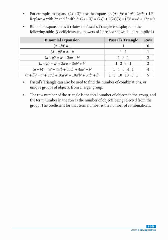
• For example, to expand (2x + 3)2, use the expansion (a + b)2 = 1a2 + 2a1b1 + 1b2. Replace a with 2x and b with 3: (2x + 3)2 = (2x)2 + 2(2x)(3) + (3)2 = 4x2 + 12x + 9.
• Binomial expansion as it relates to Pascal’s Triangle is displayed in the following table. (Coefficients and powers of 1 are not shown, but are implied.)
Binomial expansion Pascal’s Triangle Row(a + b)0 = 1 1 0
(a + b)1 = a + b 1 1 1(a + b)2 = a2 + 2ab + b2 1 2 1 2
(a + b)3 = a3 + 3a2b + 3ab2 + b3 1 3 3 1 3(a + b)4 = a4 + 4a3b + 6a2b2 + 4ab3 + b4 1 4 6 4 1 4
(a + b)5 = a5 + 5a4b + 10a3b2 + 10a2b3 + 5ab4 + b5 1 5 10 10 5 1 5
• Pascal’s Triangle can also be used to find the number of combinations, or unique groups of objects, from a larger group.
• The row number of the triangle is the total number of objects in the group, and the term number in the row is the number of objects being selected from the group. The coefficient for that term number is the number of combinations.

U2-40Unit 2: Polynomial Functions
Example 1
Use the Binomial Theorem to expand (6x + 2y)3.
1. Create Pascal’s Triangle to the appropriate row.
Note that the first line of the triangle is “row 0.” The expression (6x + 2y) is raised to the third power, so the first four rows of the triangle are needed; that is, rows 0–3.
Find the terms for each new row by adding pairs of terms in the row above.
1Row 0
Row 1
Row 2
Row 3
1
1
1
1
21
331
2. Identify the row of Pascal’s Triangle with the coefficients of the expanded expression.
The power of the binomial is 3, so the coefficients will come from row 3 of Pascal’s Triangle.
1Row 0
Row 1
Row 2
Row 3
1
1
1
1
21
331
The coefficients of the terms in row 3 are 1, 3, 3, and 1.
Guided Practice 2.2.3

U2-41Lesson 2: Proving Identities
3. Write the expanded expression with the coefficients and powers of each term.
The powers of the terms will follow the pattern a3, a2b1, a1b2, b3.
Replace a with 6x and b with 2y.
The coefficients of the terms are from row 3 of Pascal’s Triangle.
(6x)3 + 3(6x)2(2y) + 3(6x)(2y)2 + (2y)3
4. Evaluate each term.
Use the order of operations to evaluate each term, first evaluating any exponents, then finding the products.
(6x)3 + 3(6x)2(2y) + 3(6x)(2y)2 + (2y)3 Expression from the previous step
= 216x3 + 3(36x2)(2y) + 3(6x)(4y2) + 8y3 Evaluate the exponents.
= 216x3 + 216x2y + 72xy2 + 8y3 Find the products.
The expression (6x + 2y)3, when expanded, is 216x3 + 216x2y + 72xy2 + 8y3.

U2-42Unit 2: Polynomial Functions
Example 2
Find term 4 from row 6 of Pascal’s Triangle.
1. Create Pascal’s Triangle to the appropriate row.
Note that the first line of the triangle is “row 0.”
To include row 6, seven lines of Pascal’s Triangle need to be created.
Find the terms for each new row by adding pairs of terms in the row above.
1Row 0
Row 1
Row 2
Row 3
Row 4
Row 5
Row 6
1
1
1
1
1
1
1
21
331
4641
5101051
615201561
2. Find term 4 in the row.
Recall that the first term in each row is named “term 0,” so term 4 is actually the fifth term in the row.
1Row 0
Row 1
Row 2
Row 3
Row 4
Row 5
Row 6
1
1
1
1
1
1
1
21
331
4641
5101051
615201561
Term 4 from row 6 of Pascal’s Triangle is 15.

U2-43Lesson 2: Proving Identities
Example 3
Find term 4 in the expanded expression of (4x – 9y)7.
1. Identify the row of Pascal’s Triangle with the coefficients of the expanded expression.
The power of the binomial is 7, so the coefficients will come from row 7 of Pascal’s Triangle.
1Row 0
Row 1
Row 2
Row 3
Row 4
Row 5
Row 6
Row 7
1
1
1
1
1
1
1
1
21
331
4641
5101051
615201561
72135352171
The coefficients of the terms are 1, 7, 21, 35, 35, 21, 7, and 1.
2. Identify the powers of the binomial terms in term 4.
In the expression (4x – 9y)7, n = 7.
The term number, k, is 4.
The power of 4x is n – k = 7 – 4 = 3.
The power of –9y is k = 4.
U2-44Unit 2: Polynomial Functions
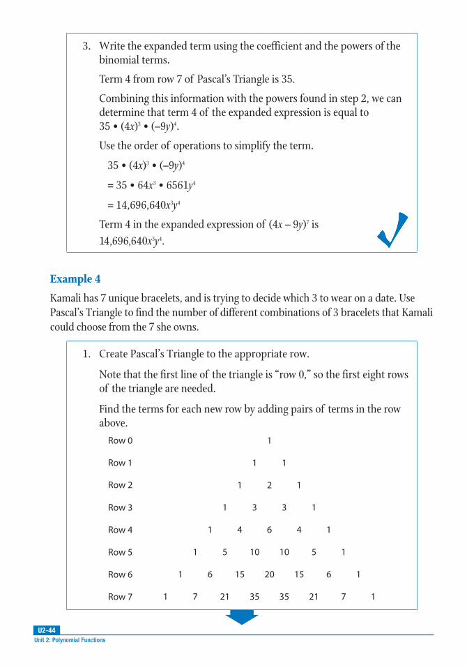
3. Write the expanded term using the coefficient and the powers of the binomial terms.
Term 4 from row 7 of Pascal’s Triangle is 35.
Combining this information with the powers found in step 2, we can determine that term 4 of the expanded expression is equal to 35 • (4x)3 • (–9y)4.
Use the order of operations to simplify the term.
35 • (4x)3 • (–9y)4
= 35 • 64x3 • 6561y4
= 14,696,640x3y4
Term 4 in the expanded expression of (4x – 9y)7 is 14,696,640x3y4.
Example 4
Kamali has 7 unique bracelets, and is trying to decide which 3 to wear on a date. Use Pascal’s Triangle to find the number of different combinations of 3 bracelets that Kamali could choose from the 7 she owns.
1. Create Pascal’s Triangle to the appropriate row.
Note that the first line of the triangle is “row 0,” so the first eight rows of the triangle are needed.
Find the terms for each new row by adding pairs of terms in the row above.
1Row 0
Row 1
Row 2
Row 3
Row 4
Row 5
Row 6
Row 7
1
1
1
1
1
1
1
1
21
331
4641
5101051
615201561
72135352171

U2-45Lesson 2: Proving Identities
2. Find term 3 in the row.
The first term in each row is named “term 0,” so term 3 is actually the fourth term in the row.
1Row 0
Row 1
Row 2
Row 3
Row 4
Row 5
Row 6
Row 7
1
1
1
1
1
1
1
1
21
331
4641
5101051
615201561
72135352171
Term 3 from row 7 of Pascal’s Triangle is 35.
There are 35 different combinations of 3 bracelets that Kamali could choose to wear out of the 7 bracelets she owns.
UNIT 2 • POLYNOMIAL FUNCTIONSLesson 2: Proving Identities
PRACTICE
U2-46Unit 2: Polynomial Functions
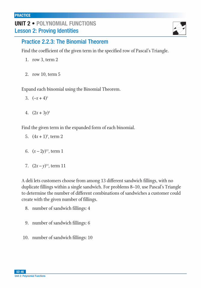
Find the coefficient of the given term in the specified row of Pascal’s Triangle.
1. row 3, term 2
2. row 10, term 5
Expand each binomial using the Binomial Theorem.
3. (–x + 4)3
4. (2x + 3y)4
Find the given term in the expanded form of each binomial.
5. (4x + 1)9, term 2
6. (x – 2y)12, term 1
7. (2x – y)14, term 11
A deli lets customers choose from among 13 different sandwich fillings, with no duplicate fillings within a single sandwich. For problems 8–10, use Pascal’s Triangle to determine the number of different combinations of sandwiches a customer could create with the given number of fillings.
8. number of sandwich fillings: 4
9. number of sandwich fillings: 6
10. number of sandwich fillings: 10
Practice 2.2.3: The Binomial Theorem

U2-47
Lesson 3: Graphing Polynomial Functions
UNIT 2 • POLYNOMIAL FUNCTIONS
Lesson 3: Graphing Polynomial Functions
Essential Questions
1. How can the degree and sign of the leading coefficient of a polynomial function be used to determine the end behavior of that function?
2. How can the degree and sign of the leading coefficient of a polynomial function be used to determine the number of turns of that function?
3. How can you use the number of sign changes in a function to determine the number and type of real zeros of that function?
4. How can synthetic substitution be used to find the value of a function?
5. How are factors, zeros, and x-intercepts of a polynomial function related?
Common Core Georgia Performance Standards
MCC9–12.N.CN.9 (+)
MCC9–12.A.APR.2
MCC9–12.A.APR.3
MCC9–12.F.IF.7c★
WORDS TO KNOW
complex conjugate the complex number that when multiplied by another complex number produces a value that is wholly real; the complex conjugate of a + bi is a – bi
Complex Conjugate Theorem
Let p(x) be a polynomial with real coefficients. If a + bi is a root of the equation p(x) = 0, where a and b are real and b ≠ 0, then a – bi is also a root of the equation.
depressed polynomial the result of dividing a polynomial by one of its binomial factors
end behavior the behavior of the graph as x approaches positive or negative infinity
U2-48Unit 2: Polynomial Functions
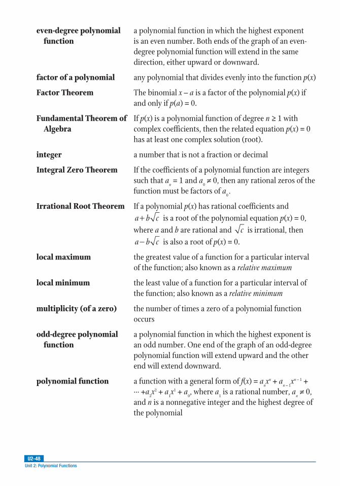
even-degree polynomial function
a polynomial function in which the highest exponent is an even number. Both ends of the graph of an even-degree polynomial function will extend in the same direction, either upward or downward.
factor of a polynomial any polynomial that divides evenly into the function p(x)
Factor Theorem The binomial x – a is a factor of the polynomial p(x) if and only if p(a) = 0.
Fundamental Theorem of Algebra
If p(x) is a polynomial function of degree n ≥ 1 with complex coefficients, then the related equation p(x) = 0 has at least one complex solution (root).
integer a number that is not a fraction or decimal
Integral Zero Theorem If the coefficients of a polynomial function are integers such that a
n = 1 and a
0 ≠ 0, then any rational zeros of the
function must be factors of a0 .
Irrational Root Theorem If a polynomial p(x) has rational coefficients and a b c+ is a root of the polynomial equation p(x) = 0, where a and b are rational and c is irrational, then a b c− is also a root of p(x) = 0.
local maximum the greatest value of a function for a particular interval of the function; also known as a relative maximum
local minimum the least value of a function for a particular interval of the function; also known as a relative minimum
multiplicity (of a zero) the number of times a zero of a polynomial function occurs
odd-degree polynomial function
a polynomial function in which the highest exponent is an odd number. One end of the graph of an odd-degree polynomial function will extend upward and the other end will extend downward.
polynomial function a function with a general form of f(x) = anxn + a
n – 1xn – 1 +
… +a2x2 + a
1x1 + a
0, where a
1 is a rational number, a
n ≠ 0,
and n is a nonnegative integer and the highest degree of the polynomial

U2-49Lesson 3: Graphing Polynomial Functions
Rational Root Theorem If the polynomial p(x) has integer coefficients, then every
rational root of the polynomial equation p(x) = 0 can be
written in the form p
q, where p is a factor of the constant
term p(x) and q is a factor of the leading coefficient of p(x).
relative maximum the greatest value of a function for a particular interval of the function; also known as a local maximum
relative minimum the least value of a function for a particular interval of the function; also known as a local minimum
Remainder Theorem For a polynomial p(x) and a number a, dividing p(x) by x – a results in a remainder of p(a), so p(a) = 0 if and only if (x – a) is a factor of p(x).
repeated root a polynomial function with a root that occurs more than once
root the x-intercept of a function; also known as zero
synthetic division a shorthand way of dividing a polynomial by a linear binomial
synthetic substitution the process of using synthetic division to evaluate a function by using only the coefficients
turning point a point where the graph of the function changes direction, from sloping upward to sloping downward or vice versa
zero the x-intercept of a function; also known as root

U2-50Unit 2: Polynomial Functions
Recommended Resources• Hotmath.com. “Rational Zeros and the Fundamental Theorem of Algebra.”
http://www.walch.com/rr/00165
This site provides numerous practice problems centering on determining the zeros of a function using the Fundamental Theorem of Algebra. Users may click to show hints and step-by-step guidance toward solutions.
• Illuminations. “Function Matching.”
http://www.walch.com/rr/00166
Given a graphed function, users manipulate this interactive applet to recreate the graph of the identical function. Users can choose the type of function to match, or match a random function generated by the site.
• MathIsFun.com. “Remainder Theorem and Factor Theorem.”
http://www.walch.com/rr/00167
This site summarizes both the Remainder Theorem and the Factor Theorem, and features examples as well as practice problems with worked solutions.
• Purplemath.com. “Solving Polynomials.”
http://www.walch.com/rr/00168
This site offers a summary of solving large polynomials in addition to information on factoring and graphing polynomial functions.

U2-51Lesson 3: Graphing Polynomial Functions
IntroductionBy this point in your mathematics experience, you have worked extensively with functions: determining the slopes of linear functions, identifying the vertices of quadratic functions as maxima or minima, determining the end behavior of exponential functions, and identifying intercepts of many types of functions. You can extend the skills you have used to analyze functions you have previously studied in order to understand the graphs of other polynomial functions.
Key Concepts
• Recall that a polynomial function is a function with a general form of f(x) = anxn
+ an – 1
xn – 1 + … + a2x2 + a
1x1 + a
0, where a
1 is a rational number, a
n ≠ 0, and n
is the
highest degree of the polynomial.
• Polynomial functions are defined for any function that contains positive integer exponents.
• Recall that integers are numbers that are not fractions or decimals.
• The degree of a polynomial function is the highest exponent to which the dependent variable is raised.
• For example, the equation y = 3x7 + 9x3 – x + 4 is a seventh-degree polynomial function because its highest exponent is 7 and all other exponents are positive whole numbers.
• 4 6 33
5y x x= + − is not a polynomial function because the exponent is not
a whole number. 3 4y x=− + is also not a polynomial function since the
square root of a number can be written as a power of 1
2, which is not a whole
number either. And 5 2 63 4y x x= + +− is not a polynomial function because
not all exponents are non-negative integers.
End Behavior
• To determine the end behavior of a polynomial function, or the behavior of the graph as x approaches positive or negative infinity, consider the highest degree of the polynomial and its coefficient, axn.
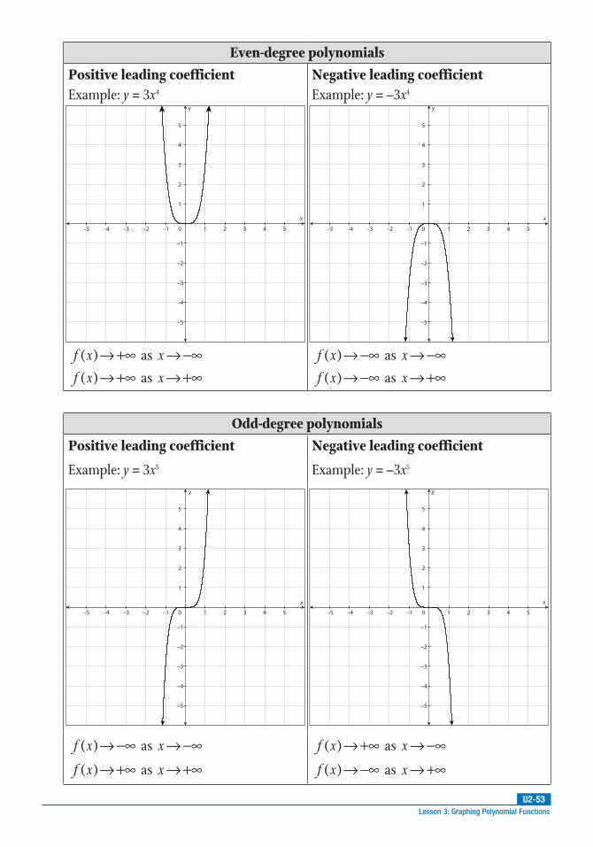
• If n is even, the polynomial function is considered an even-degree polynomial function.
Lesson 2.3.1: Describing End Behavior and Turns
U2-52Unit 2: Polynomial Functions
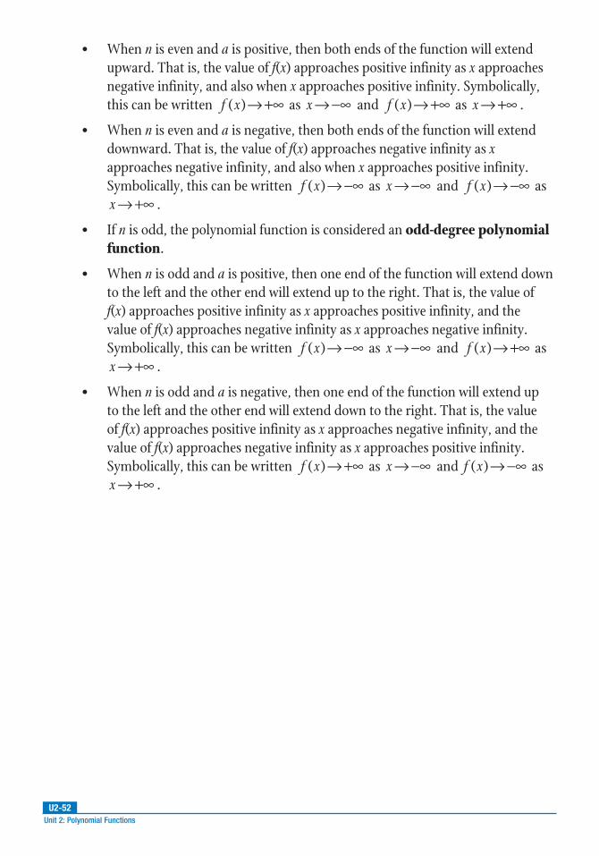
• When n is even and a is positive, then both ends of the function will extend upward. That is, the value of f(x) approaches positive infinity as x approaches negative infinity, and also when x approaches positive infinity. Symbolically, this can be written ( )f x →+∞ as x→−∞ and ( )f x →+∞ as x→+∞ .
• When n is even and a is negative, then both ends of the function will extend downward. That is, the value of f(x) approaches negative infinity as x approaches negative infinity, and also when x approaches positive infinity. Symbolically, this can be written ( )f x →−∞ as x→−∞ and ( )f x →−∞ as x→+∞ .
• If n is odd, the polynomial function is considered an odd-degree polynomial function.
• When n is odd and a is positive, then one end of the function will extend down to the left and the other end will extend up to the right. That is, the value of f(x) approaches positive infinity as x approaches positive infinity, and the value of f(x) approaches negative infinity as x approaches negative infinity. Symbolically, this can be written ( )f x →−∞ as x→−∞ and ( )f x →+∞ as x→+∞ .
• When n is odd and a is negative, then one end of the function will extend up to the left and the other end will extend down to the right. That is, the value of f(x) approaches positive infinity as x approaches negative infinity, and the value of f(x) approaches negative infinity as x approaches positive infinity. Symbolically, this can be written ( )f x →+∞ as x→−∞ and ( )f x →−∞ as x→+∞ .
U2-53Lesson 3: Graphing Polynomial Functions
Even-degree polynomialsPositive leading coefficientExample: y = 3x4
Negative leading coefficientExample: y = –3x4
–5 –4 –3 –2 –1 0 1 2 3 4 5
–5
–4
–3
–2
–1
1
2
3
4
5
–5 –4 –3 –2 –1 0 1 2 3 4 5
–5
–4
–3
–2
–1
1
2
3
4
5
( )f x →+∞ as x→−∞( )f x →+∞ as x→+∞
( )f x →−∞ as x→−∞( )f x →−∞ as x→+∞
Odd-degree polynomialsPositive leading coefficient
Example: y = 3x5
Negative leading coefficient
Example: y = –3x5
–5 –4 –3 –2 –1 0 1 2 3 4 5
–5
–4
–3
–2
–1
1
2
3
4
5
–5 –4 –3 –2 –1 0 1 2 3 4 5
–5
–4
–3
–2
–1
1
2
3
4
5
( )f x →−∞ as x→−∞
( )f x →+∞ as x→+∞( )f x →+∞ as x→−∞
( )f x →−∞ as x→+∞
U2-54Unit 2: Polynomial Functions
Turning Points
• A turning point of a function is a point where the graph of the function changes from sloping upward to sloping downward or, alternatively, from sloping downward to sloping upward.
• To determine the maximum number of turning points of a function, subtract 1 from the highest degree of the polynomial. In other words, find n – 1.
• For instance, the polynomial function y = 3x7 + 9x3 – x + 4 can have no more than 7 – 1, or 6, turning points.
• The maximum number of turning points does not necessarily indicate the actual number of turning points of a function, just that it can have no more than that number. Some functions may have fewer turning points than the number calculated.
• A turning point corresponds to a local maximum, the greatest value of a function for a particular interval of the function, or a local minimum, the least value of a function for a particular interval of the function. A local maximum may also be referred to as a relative maximum and a local minimum may also be referred to as a relative minimum.
Roots of a Polynomial Function
• The highest degree of the polynomial determines the maximum number of roots, or x-intercepts of a function.
• A polynomial function with a degree of 10 could have up to 10 roots, but could also have 0 to 9 roots, depending on the specific equation.
• Recall that real numbers include all rational and irrational numbers, but do not include imaginary and complex numbers.
Sketching a Polynomial Function
• Being able to identify the general end behavior, the possible number of turning points, and the maximum number of roots of a polynomial function can be helpful in creating a rough sketch of the function.
• Start by choosing at least six x-values that are both positive and negative. It is also useful to choose the value of 0.
• As you’ve done in previous courses, substitute each chosen x-value into the given function and evaluate to determine the corresponding y-value. Then, plot the points on a graph.

U2-55Lesson 3: Graphing Polynomial Functions
• Be sure to smoothly connect all chosen points to illustrate the graph of the function.
• Graphing calculators are especially helpful when sketching a complicated function.

U2-56Unit 2: Polynomial Functions
Guided Practice 2.3.1
Example 1
Determine the end behavior, maximum number of turning points, and maximum number of real roots of the function f(x) = 6x5 – 3x4 + 2x + 7.
1. Identify the leading coefficient and degree of the polynomial function.
The function f(x) = 6x5 – 3x4 + 2x + 7 is a fifth-degree polynomial function because the highest exponent is 5.
The coefficient of the term containing the highest exponent is 6; therefore, 6 is the leading coefficient.
2. Determine the end behavior of the function.
The leading coefficient, 6, is positive and the degree of the function, 5, is odd; therefore, the graph of the function will extend down to the left and up to the right.
Symbolically, ( )f x →−∞ as x→−∞ and ( )f x →+∞ as x→+∞ .
3. Determine the maximum number of turning points of the polynomial function.
To determine the maximum number of turning points, subtract 1 from the degree of the polynomial; that is, find n – 1.
The degree of the polynomial is 5, and 5 – 1 = 4.
The maximum number of turning points in the graph is 4.
4. Determine the maximum number of real roots of the polynomial function.
The maximum number of real roots is equal to the degree of the polynomial; therefore, the maximum number of roots of the function f(x) = 6x5 – 3x4 + 2x + 7 is 5.
U2-57Lesson 3: Graphing Polynomial Functions
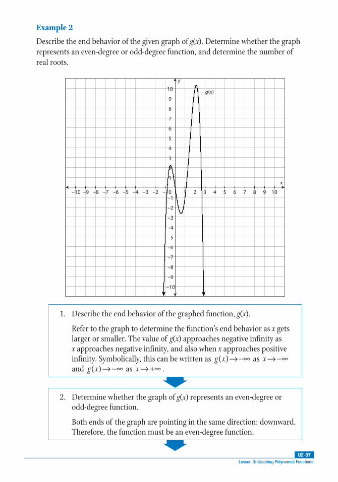
Example 2
Describe the end behavior of the given graph of g(x). Determine whether the graph represents an even-degree or odd-degree function, and determine the number of real roots.
–10 –9 –8 –7 –6 –5 –4 –3 –2 –10 1 2 3 4 5 6 7 8 9 10
–10
–9
–8
–7
–6
–5
–4
–3
–2
–1
1
2
3
4
5
6
7
8
9
10 g(x)
1. Describe the end behavior of the graphed function, g(x).
Refer to the graph to determine the function’s end behavior as x gets larger or smaller. The value of g(x) approaches negative infinity as x approaches negative infinity, and also when x approaches positive infinity. Symbolically, this can be written as ( )g x →−∞ as x→−∞ and ( )g x →−∞ as x→+∞ .
2. Determine whether the graph of g(x) represents an even-degree or odd-degree function.
Both ends of the graph are pointing in the same direction: downward. Therefore, the function must be an even-degree function.

U2-58Unit 2: Polynomial Functions
3. Determine the number of real roots.
Real roots are the points at which the graphed function intersects the x-axis. Because the x-axis contains only real numbers, only the real roots can be graphed. Determine the number of times the graph intersects the x-axis.
–10 –9 –8 –7 –6 –5 –4 –3 –2 –10 1 2 3 4 5 6 7 8 9 10
–10
–9
–8
–7
–6
–5
–4
–3
–2
–1
1
2
3
4
5
6
7
8
9
10 g(x)
The graph intersects the x-axis at four points, so there are four real roots.
U2-59Lesson 3: Graphing Polynomial Functions
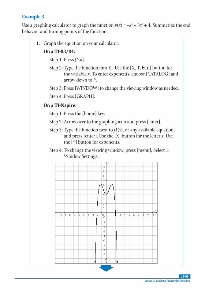
Example 3
Use a graphing calculator to graph the function p(x) = –x4 + 3x2 + 4. Summarize the end behavior and turning points of the function.
1. Graph the equation on your calculator.
On a TI-83/84:
Step 1: Press [Y=].
Step 2: Type the function into Y1. Use the [X, T, θ, n] button for
the variable x. To enter exponents, choose [CATALOG] and arrow down to ^.
Step 3: Press [WINDOW] to change the viewing window as needed.
Step 4: Press [GRAPH].
On a TI-Nspire:
Step 1: Press the [home] key.
Step 2: Arrow over to the graphing icon and press [enter].
Step 3: Type the function next to f1(x), or any available equation, and press [enter]. Use the [X] button for the letter x. Use the [^] button for exponents.
Step 4: To change the viewing window, press [menu]. Select 1: Window Settings.
–10 –9 –8 –7 –6 –5 –4 –3 –2 –10 1 2 3 4 5 6 7 8 9 10
–10
–9
–8
–7
–6
–5
–4
–3
–2
–1
1
2
3
4
5
6
7
8
9
10

U2-60Unit 2: Polynomial Functions
2. Analyze the table of values.
Refer to the table of values for the function.
On a TI-83/84:
Step 1: Choose [TABLE]. Scroll up and down the table to view various points on the graph.
On a TI-Nspire:
Step 1: Choose [menu]. Navigate to 7: Table, 1: Split-Screen Table. Arrow up and down the table to view various points on the graph.
Points include:
x y–3 –50–2 0–1 60 41 62 03 –50
Both ends of the graph extend in the same direction, and the graph opens downward. Therefore, we know that this is an even-degree polynomial with a negative leading coefficient, so ( )p x →−∞ as x→−∞ , and ( )p x →−∞ as x→+∞ .
We can see from the graph that this function has three turning points. It can be seen from the graph and the table of values that one turning point is at (0, 4). x = 0 is less than the surrounding points, so it is a local (or relative) minimum. Two other approximate turning points are (–1, 6) and (1, 6). x = –1 and 1 are greater than the surrounding points, so they are both local (or relative) maximums.
The graph intersects the x-axis at two points, indicating that there are two real roots of this function.
U2-61Lesson 3: Graphing Polynomial Functions
Example 4
Create a rough sketch of the graph of a sixth-degree polynomial function with a positive leading coefficient.
1. Determine the end behavior of the possible function.
The function is a sixth-degree polynomial; therefore, it is an even-degree polynomial. Both ends of the graphed function will extend in the same direction. Because the leading coefficient is positive, both ends of the graphed function will extend upward. Symbolically,
( )f x →+∞ as x→−∞ and ( )f x →+∞ as x→+∞ .
2. Determine the maximum number of turns.
The maximum number of turns is defined by the degree of the polynomial minus 1.
maximum number of turns = n – 1
= 6 – 1
= 5
A sixth-degree polynomial will have no more than 5 turning points.
3. Determine the maximum number of real roots.
The maximum number of real roots, or x-intercepts, is equal to the degree of the polynomial. This particular function will have no more than 6 real roots.
U2-62Unit 2: Polynomial Functions
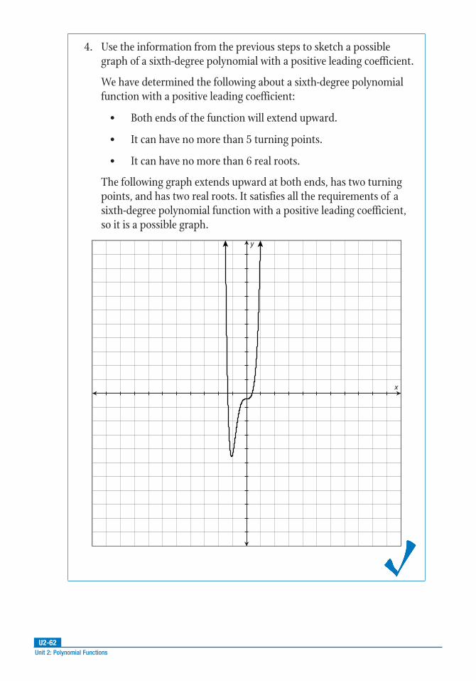
4. Use the information from the previous steps to sketch a possible graph of a sixth-degree polynomial with a positive leading coefficient.
We have determined the following about a sixth-degree polynomial function with a positive leading coefficient:
• Both ends of the function will extend upward.
• It can have no more than 5 turning points.
• It can have no more than 6 real roots.
The following graph extends upward at both ends, has two turning points, and has two real roots. It satisfies all the requirements of a sixth-degree polynomial function with a positive leading coefficient, so it is a possible graph.

UNIT 2 • POLYNOMIAL FUNCTIONSLesson 3: Graphing Polynomial Functions
PRACTICE
U2-63Lesson 3: Graphing Polynomial Functions
Practice 2.3.1: Describing End Behavior and TurnsFor problems 1 and 2, determine the end behavior, the maximum number of turning points, and the maximum number of real roots of each function.
1. ( ) 5 3 2 67 4g x x x x=− + − +
2. ( ) 7 2 5 88 3f x x x x= + − −
For problems 3 and 4, describe the end behavior of each graph. Determine whether the graph represents an even-degree or odd-degree function, and determine the number of real roots.
3. f(x)
4.
f(x)
For problems 5 and 6, create a rough sketch of a possible graph of the function described.
5. a ninth-degree polynomial with a positive leading coefficient
6. an eighth-degree polynomial with a negative leading coefficient
continued

UNIT 2 • POLYNOMIAL FUNCTIONSLesson 3: Graphing Polynomial Functions
PRACTICE
U2-64Unit 2: Polynomial Functions
The following graph models the volume of water in a water reservoir each year since 1900. Use this graph to complete problems 7–10.
10 20 30 40 50 60 70 80 90 100
25
50
75
100
125
150
175
200
225
250
275
300
325
350
375
400
S(t)
Years since 1900
Volu
me
(gal
lons
)
7. Estimate the turning points of the graph of this function.
8. What do the turning points mean in terms of the volume of the reservoir?
9. Describe the end behavior of this graph.
10. If this graph were modeled by a polynomial function, what is the least degree the equation could have? Explain your answer.

U2-65Lesson 3: Graphing Polynomial Functions
Lesson 2.3.2:
IntroductionIn mathematics, the word “remainder” is often used in relation to the process of long division. You are probably familiar with dividing whole numbers. For example, the result (or quotient) of 8 divided by 4 is 2; that is, 8 ÷ 4 = 2. In other words, if the dividend of 8 units were divided by a divisor of 4, each group would have 2 units.
The process of division does not always result in a whole number. For instance, the
result of 14 divided by 5, or 14 ÷ 5, is 2 with a remainder of 4. Recall that this means
that if a dividend of 14 units were divided by a divisor of 5, then each group would have
2 units and there would be 4 units left over. 4 is referred to as the remainder. In earlier
grades, you often wrote the quotient and its remainder as 2R4 or 24
5. The idea of
having remainders also extends to dividing polynomials. Sometimes when polynomials
are divided, the result is a polynomial; other times there is a remainder.
Key Concepts
• Long division, used to divide whole numbers, can also be used to divide polynomials. Recall that the dividend is the quantity being divided, and the divisor is the quantity by which it is being divided: dividend ÷ divisor = quotient.
• Long division with polynomials can sometimes be long and tedious; fortunately, there is another way to divide polynomials.
• The process of synthetic division, a shorthand way of dividing a polynomial by a linear binomial by using only the coefficients, is often used instead.
• In order to use synthetic division, the dividend must be a polynomial written in standard form, ordered by the power of the variables, with the largest power listed first. If a term is missing, 0 must be used in its place.
• For example, compare 4x2 + 16 to the standard form of a polynomial, a
nxn + a
n – 1xn – 1 + … + a
2x2 + a
1x1 + a
0. Notice that 4x2 + 16 does not have a value for
an – 1
xn – 1, or in this case, ax. To prepare this polynomial for synthetic division, substitute 0 as the coefficient (a) in the ax term: 4x2 + 0x + 16. Now you can use the coefficients 4, 0, and 16 to perform the synthetic division.
• For synthetic division, the divisor must be of the form (x – a), where a is a real number.
Lesson 2.3.2: The Remainder Theorem

U2-66Unit 2: Polynomial Functions
• Use the following steps to divide polynomials using synthetic division. An example has been provided for clarity.
Synthetic Division of Polynomials
Example: (3x2 – 20x + 12) ÷ (x – 3)1. Write the coefficients of the dividend,
3x2 – 20x + 12: 3, –20, and 12. 3 20 12−
2. Identify the value of a in the divisor, (x – a). Write this value, 3, in the upper left corner.
3 3 20 12−
3. Create a horizontal line below the coefficients, allowing for space to write above and below the line.
3 3 20 12−
4. Write the first coefficient in the dividend below the horizontal line.
3 3 20 12
3
−
5. Multiply the number below the horizontal line by the value of a and write the product under the next coefficient and above the horizontal line.
3 3 20 12
9
3
−
6. Add the numbers in the new column. Write the result below the horizontal line in that column.
3 3 20 12
9
3 11
−
−7. Repeat steps 5 and 6 until addition has been
completed for all columns.3 3 20 12
9 33
3 11 21
−−
− −8. Draw a box around the far right sum. 3 3 20 12
9 33
3 11 21
−−
− −9. The numbers below the horizontal line represent
the quotient. These numbers are the coefficients of the polynomial quotient in the order of decreasing degree. The boxed number is the remainder. Place the remainder over the divisor to express the final term of the polynomial.
3 1121
3x
x= − −
−

U2-67Lesson 3: Graphing Polynomial Functions
• If you are dividing by a linear function, (x – a), the order of the quotient is 1 less than the dividend. The remainder, if any, is a constant.
• If the remainder is 0, then the divisor is a factor of the polynomial.
• Synthetic division can also be used to find the value of a function. This is known as synthetic substitution.
• To evaluate a polynomial using synthetic substitution, follow the same process described for synthetic division. For example, given the function 3x2 – 20x + 12, if you must determine the value of the function at x = 3, use 3 as the a value in the divisor of the synthetic division. The resulting remainder gives the value of the polynomial when evaluated at x = 3.
• If a polynomial p(x) is divided by (x – a), then the remainder, r, is equal to p(a).
• This process leads to the Remainder Theorem.
Remainder TheoremFor a polynomial p(x) and a number a, dividing p(x) by x – a results in a remainder of p(a), so p(a) = 0 if and only if (x – a) is a factor of p(x).
• To take a closer look at the Remainder Theorem, let’s work with the same polynomial we used to demonstrate synthetic division of polynomials: 3x2 – 20x + 12.
• Let p(x) = 3x2 – 20x + 12. We can use synthetic substitution (by following the process of synthetic division), to evaluate this function for x = 3. The result is the remainder, or –21. Because this result is a number other than 0, the Remainder Theorem allows us to conclude that (x – 3) is not a factor of p(x). Only when the remainder is 0 will (x – a) be a factor of the polynomial. A remainder of any number other than 0 indicates that (x – a) is not a factor of the given polynomial.
• If we evaluate the same function, p(x) = 3x2 – 20x + 12, for x = 6, the remainder is 0. By the Remainder Theorem, (x – 6) is a factor of the given polynomial.
• Dividing a polynomial by one of its binomial factors results in a depressed polynomial. When 3x2 – 20x + 12 is divided by 6, the depressed polynomial is 3x – 2.

U2-68Unit 2: Polynomial Functions
• It is sometimes easier to evaluate a function for a given value by using direct substitution. For instance, when evaluating the expression 3x2 + 2 when x = 4, directly substitute 4 into the polynomial and follow the order of operations: 3(4)2 + 2 = 3(16) + 2 = 48 + 2 = 50. Other times, when the polynomials are more complicated, synthetic substitution is more efficient. Both methods are helpful when working with polynomials.
• As you will see in this lesson, synthetic division and substitution can also be applied to real-world problems.

U2-69Lesson 3: Graphing Polynomial Functions
Example 1
Find the quotient of (x2 – 5x – 20) ÷ (x – 4) using polynomial long division.
1. Set up the division.
The dividend is x2 – 5x – 20 and the divisor is x – 4.
)4 5 202x x x− − −
2. Divide the leading term of the dividend by the leading term of the divisor.
The leading term of the dividend is x2. The leading term of the divisor is x.
The result of x2 divided by x is x.
Record the result in a manner similar to long division of whole numbers.
)4 5 202x x xx
− − −
Multiply the result, x, by the divisor, x – 4.
x(x – 4) = x2 – 4x
Write the result under the dividend, lining up the terms of equal degree.
)4 5 20
4
2
2
x x xx
x x
− − −
−
Subtract the last line from the line above it.
(x2 – 5x – 20) – (x2 – 4x) = –x – 20
Record the result in the division.
)4 5 20
4
20
2
2
x x xx
x x
x
− − −
−− − (continued)
Guided Practice 2.3.2
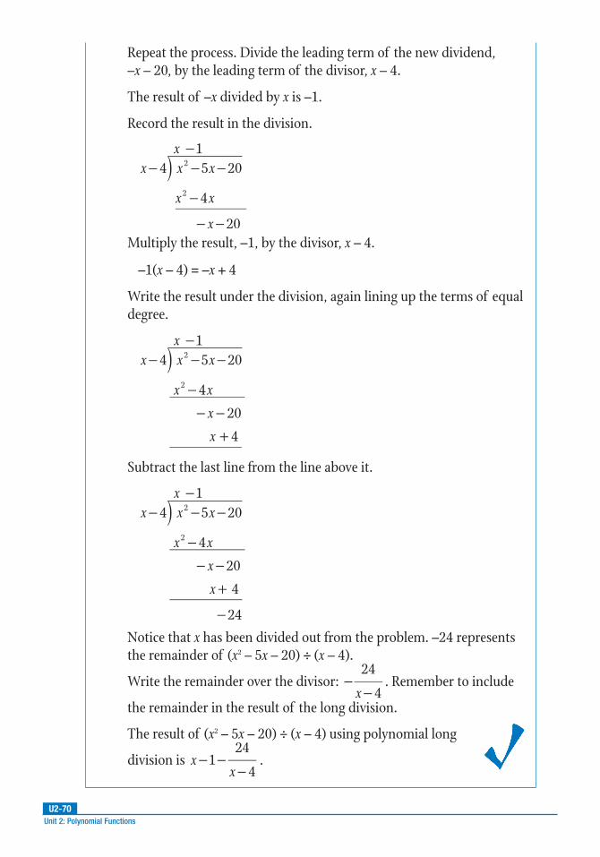
U2-70Unit 2: Polynomial Functions
Repeat the process. Divide the leading term of the new dividend, –x – 20, by the leading term of the divisor, x – 4.
The result of –x divided by x is –1.
Record the result in the division.
)4 5 201
4
20
2
2
x x xx
x x
x
− − −−
−
− −Multiply the result, –1, by the divisor, x – 4.
–1(x – 4) = –x + 4
Write the result under the division, again lining up the terms of equal degree.
)4 5 201
4
20
4
2
2
x x xx
x x
x
x
− − −−
−− −
+
Subtract the last line from the line above it.
)4 5 201
4
20
4
24
2
2
x x xx
x x
x
x
− − −−
−− −
+
−Notice that x has been divided out from the problem. –24 represents the remainder of (x2 – 5x – 20) ÷ (x – 4).
Write the remainder over the divisor: 24
4x−
−. Remember to include
the remainder in the result of the long division.
The result of (x2 – 5x – 20) ÷ (x – 4) using polynomial long
division is 124
4x
x− −
−.
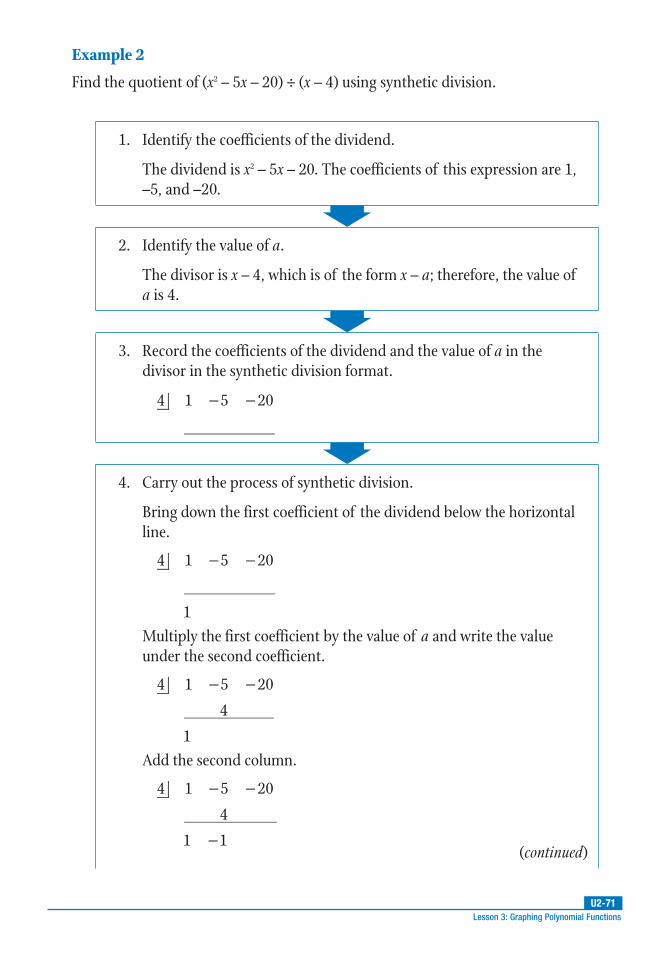
U2-71Lesson 3: Graphing Polynomial Functions
Example 2
Find the quotient of (x2 – 5x – 20) ÷ (x – 4) using synthetic division.
1. Identify the coefficients of the dividend.
The dividend is x2 – 5x – 20. The coefficients of this expression are 1, –5, and –20.
2. Identify the value of a.
The divisor is x – 4, which is of the form x – a; therefore, the value of a is 4.
3. Record the coefficients of the dividend and the value of a in the divisor in the synthetic division format.
4 1 5 20− −
4. Carry out the process of synthetic division.
Bring down the first coefficient of the dividend below the horizontal line.
4 1 5 20
1
− −
Multiply the first coefficient by the value of a and write the value under the second coefficient.
4 1 5 20
4
1
− −
Add the second column.
4 1 5 20
4
1 1
− −
−(continued)

U2-72Unit 2: Polynomial Functions
Continue multiplying and adding for the remaining column.
4 1 5 20
4 4
1 1 24
− −−
− −Draw a box around the remainder.
4 1 5 20
4 4
1 1 24
− −−
− −
5. Write the quotient.
Each sum represents the coefficient of the quotient.
Recall that the order of the quotient is 1 less than the dividend, x2.
Write the remainder over the divisor.
The result of (x2 – 5x – 20) ÷ (x – 4) using synthetic division is
124
4x
x− −
−.
Example 3
Find the quotient of (3x3 + 16x2 + 18x + 8) ÷ (x + 4) using synthetic division.
1. Identify the coefficients of the dividend.
The dividend is 3x3 + 16x2 + 18x + 8. The coefficients of this expression are 3, 16, 18, and 8.
2. Identify the value of a.
Recall that, in general, the divisor is written in the form (x – a). Here, the divisor is written as (x + 4) or [x – (– 4)]; therefore, the value of a is –4.
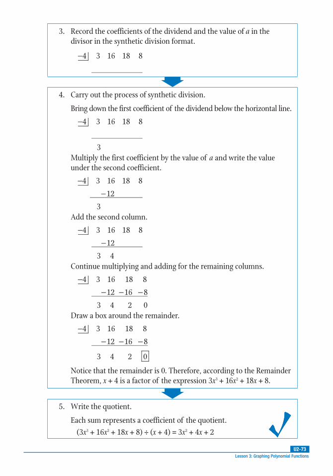
U2-73Lesson 3: Graphing Polynomial Functions
3. Record the coefficients of the dividend and the value of a in the divisor in the synthetic division format.
4 3 16 18 8−
4. Carry out the process of synthetic division.
Bring down the first coefficient of the dividend below the horizontal line.
4 3 16 18 8
3
−
Multiply the first coefficient by the value of a and write the value under the second coefficient.
4 3 16 18 8
12
3
−−
Add the second column.
4 3 16 18 8
12
3 4
−−
Continue multiplying and adding for the remaining columns.
4 3 16 18 8
12 16 8
3 4 2 0
−− − −
Draw a box around the remainder.
4 3 16 18 8
12 16 8
3 4 2 0
−− − −
Notice that the remainder is 0. Therefore, according to the Remainder Theorem, x + 4 is a factor of the expression 3x3 + 16x2 + 18x + 8.
5. Write the quotient.
Each sum represents a coefficient of the quotient. (3x3 + 16x2 + 18x + 8) ÷ (x + 4) = 3x2 + 4x + 2

U2-74Unit 2: Polynomial Functions
Example 4
Use synthetic substitution to evaluate p(x) = x2 – 32 for x = –7.
1. Identify the coefficients of the polynomial function.
The polynomial function is p(x) = x2 – 32. The coefficients of this function are 1 and –32.
2. Use synthetic division to evaluate the function for x = –7.
Write the divisor in the form x – a.
The value of x is –7; therefore, it is written as (x – a) = [x – (– 7)] or x + 7.
Determine the coefficients of the dividend.
Compare x2 – 32 to the standard form of a polynomial, anxn + a
n – 1xn – 1 +
… + a2x2 + a
1x1 + a
0. Notice that x2 – 32 does not have a value for
an – 1
xn – 1, or in this case, ax. Therefore, be sure to include 0 in the setup of the synthetic division to represent the missing coefficient.
The other coefficients are 1 and –32.
Record the coefficients of the dividend and the value of a in the divisor in the synthetic division format.
7 1 0 32− −
Work through the process of synthetic division.
7 1 0 32
7 49
1 7 17
− −−−
Draw a box around the remainder.
7 1 0 32
7 49
1 7 17
− −−
−

U2-75Lesson 3: Graphing Polynomial Functions
3. Identify the value of p(x) when x = –7.
The remainder of the synthetic division is the value of p(x) for the given value of x.
The value of p(–7) is equal to 17, the remainder found using synthetic division.
4. Verify your answer by substituting –7 for x in the polynomial function p(x) = x2 – 32.
p(x) = x2 – 32 Original function
p(–7) = (–7)2 – 32 Substitute –7 for x.
p(–7) = 49 – 32 Simplify.
p(–7) = 17
The process of synthetic substitution reveals the same answer as direct substitution.
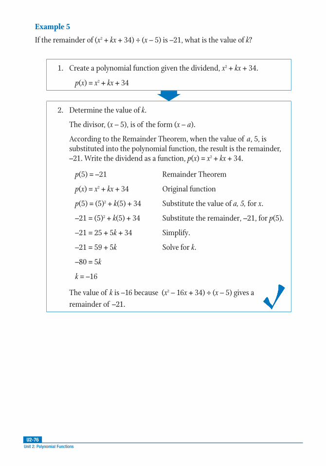
U2-76Unit 2: Polynomial Functions
Example 5
If the remainder of (x2 + kx + 34) ÷ (x – 5) is –21, what is the value of k?
1. Create a polynomial function given the dividend, x2 + kx + 34.
p(x) = x2 + kx + 34
2. Determine the value of k.
The divisor, (x – 5), is of the form (x – a).
According to the Remainder Theorem, when the value of a, 5, is substituted into the polynomial function, the result is the remainder, –21. Write the dividend as a function, p(x) = x2 + kx + 34.
p(5) = –21 Remainder Theorem
p(x) = x2 + kx + 34 Original function
p(5) = (5)2 + k(5) + 34 Substitute the value of a, 5, for x.
–21 = (5)2 + k(5) + 34 Substitute the remainder, –21, for p(5).
–21 = 25 + 5k + 34 Simplify.
–21 = 59 + 5k Solve for k.
–80 = 5k
k = –16
The value of k is –16 because (x2 – 16x + 34) ÷ (x – 5) gives a remainder of –21.
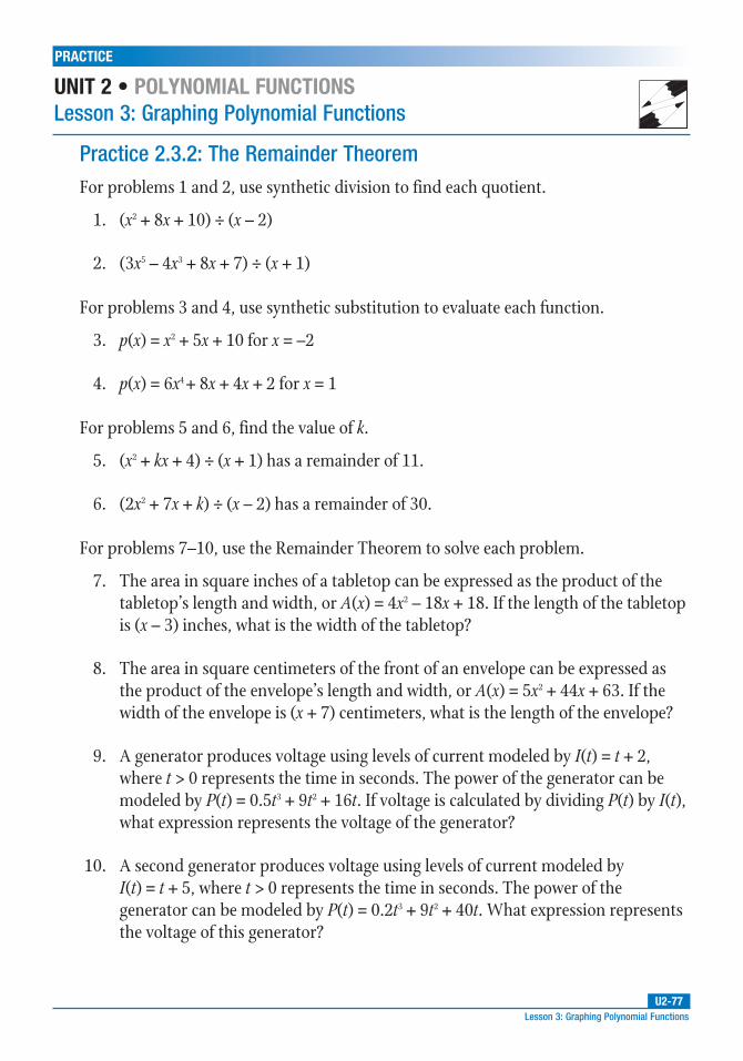
UNIT 2 • POLYNOMIAL FUNCTIONSLesson 3: Graphing Polynomial Functions
PRACTICE
U2-77Lesson 3: Graphing Polynomial Functions
For problems 1 and 2, use synthetic division to find each quotient.
1. (x2 + 8x + 10) ÷ (x – 2)
2. (3x5 – 4x3 + 8x + 7) ÷ (x + 1)
For problems 3 and 4, use synthetic substitution to evaluate each function.
3. p(x) = x2 + 5x + 10 for x = –2
4. p(x) = 6x4 + 8x + 4x + 2 for x = 1
For problems 5 and 6, find the value of k.
5. (x2 + kx + 4) ÷ (x + 1) has a remainder of 11.
6. (2x2 + 7x + k) ÷ (x – 2) has a remainder of 30.
For problems 7–10, use the Remainder Theorem to solve each problem.
7. The area in square inches of a tabletop can be expressed as the product of the tabletop’s length and width, or A(x) = 4x2 – 18x + 18. If the length of the tabletop is (x – 3) inches, what is the width of the tabletop?
8. The area in square centimeters of the front of an envelope can be expressed as the product of the envelope’s length and width, or A(x) = 5x2 + 44x + 63. If the width of the envelope is (x + 7) centimeters, what is the length of the envelope?
9. A generator produces voltage using levels of current modeled by I(t) = t + 2, where t > 0 represents the time in seconds. The power of the generator can be modeled by P(t) = 0.5t3 + 9t2 + 16t. If voltage is calculated by dividing P(t) by I(t), what expression represents the voltage of the generator?
10. A second generator produces voltage using levels of current modeled by I(t) = t + 5, where t > 0 represents the time in seconds. The power of the generator can be modeled by P(t) = 0.2t3 + 9t2 + 40t. What expression represents the voltage of this generator?
Practice 2.3.2: The Remainder Theorem

U2-78Unit 2: Polynomial Functions
IntroductionSynthetic division, along with your knowledge of end behavior and turning points, can be used to identify the x-intercepts of a polynomial function. This information allows for more accurate sketches of functions.
Key Concepts
• Recall that roots are the x-intercepts of a function. In other words, these are the x-values for which a function equals 0. These zeros are another way of referring to the roots of a function.
• When a polynomial equation with a degree greater than 0 is solved, it may have one or more real solutions, or it may have no real solutions (in which case it would have complex solutions).
• Recall that both real and imaginary numbers belong to the set of complex numbers; therefore, all polynomial functions with a degree greater than 0 will have at least one root in the set of complex numbers. This is referred to as the Fundamental Theorem of Algebra.
Fundamental Theorem of AlgebraIf p(x) is a polynomial function of degree n ≥ 1 with complex coefficients, then the related equation p(x) = 0 has at least one complex solution (root).
• A repeated root is a root that occurs more than once in a polynomial function.
• Recall that the solutions to a quadratic equation that contains imaginary numbers come in pairs. These are called complex conjugates, the complex number that when multiplied by another complex number produces a value that is wholly real; the complex conjugate of a + bi is a – bi.
• If an imaginary number is a zero of a function, its conjugate is also a zero of that function. This is true for all polynomial functions, and is known as the Complex Conjugate Theorem.
Complex Conjugate TheoremLet p(x) be a polynomial with real coefficients. If a + bi is a root of the equation p(x) = 0, where a and b are real and b ≠ 0, then a – bi is also a root of the equation.
Lesson 2.3.3: Finding Zeros

U2-79Lesson 3: Graphing Polynomial Functions
• For a polynomial function p(x), the factor of a polynomial is any polynomial that divides evenly into that function. Recall that when a polynomial is divided by one of its factors, there is a remainder of 0 and the result is a depressed polynomial. This is an illustration of the Factor Theorem.
Factor TheoremThe binomial x – a is a factor of the polynomial p(x) if and only if p(a) = 0, where a is a real number.
• The Factor Theorem can help to find all the factors of a polynomial.
• To do this, first show that the binomial in question is a factor of the polynomial. If the remainder is 0, then the binomial is a factor.
• Then, determine if the resulting depressed polynomial can be factored.
• The identified factors indicate where the function crosses the x-axis.
• The zeros of a function are related to the factors of the polynomial. The graph of a polynomial function shows the zeros of the function, which are the x-intercepts of the graph.
• It is often helpful to know which integer values of a to try when determining p(a) = 0.
• Use the Integral Zero Theorem to determine the zeros of a polynomial function.
• Identify the factors of the constant term of a polynomial function and use substitution to determine if each number results in a zero.
• Use synthetic division to determine the remaining factors.
Integral Zero Theorem If the coefficients of a polynomial function are integers such that a
n = 1
and a0 ≠ 0, then any rational zeros of the function must be factors of a
0.
• For example, consider the equation p(x) = x2 + 10x + 25. an = 1 and a
0 = 25. A
possible zero of this function is –5 because –5 is a factor of 25.
• The zeros of any polynomial function correspond to the x-intercepts of the graph and to the roots of the corresponding equation.
• If a polynomial has a factor x – a that is repeated n times, then the root is called a repeated root and x = a is a zero of multiplicity. Multiplicity refers to the number of times a zero of a polynomial function occurs.

U2-80Unit 2: Polynomial Functions
• If the multiplicity is odd, then the graph intersects the x-axis at the point (x, 0). If the multiplicity is even, then the graph just touches the axis at the point (x, 0).
• If p(x) is a polynomial with real coefficients whose terms are arranged in descending powers of the variable, then the number of positive zeros of y = p(x) is the same as the number of sign changes of the coefficients of the terms, or is less than this by an even number. Recall that when solving a quadratic function, we used the quadratic formula, which generated pairs of roots. Often, these roots were complex and the x-intercepts could not be graphed on the coordinate plane. For this reason, we must count down from our maximum number of zeros by twos to determine the number of real zeros. For example, for a polynomial with 3 sign changes, the number of positive zeros may be 3 or 1, since 3 – 2 = 1.
• Also, the number of negative zeros of y = p(x) is the same as the number of sign changes of the coefficients of the terms of p(–x), or is less than this number by an even number.
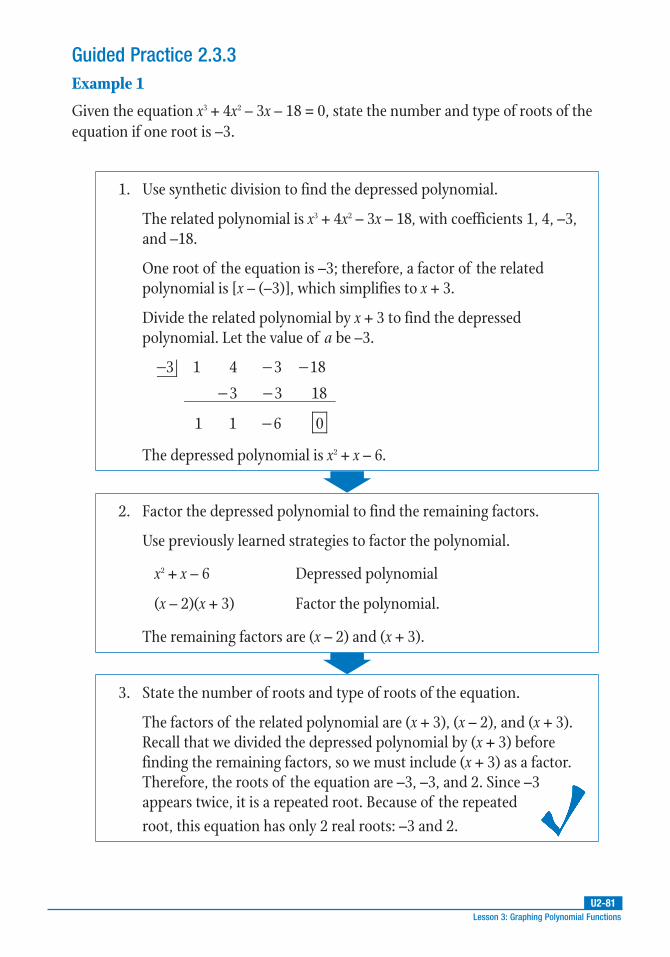
U2-81Lesson 3: Graphing Polynomial Functions
Guided Practice 2.3.3Example 1
Given the equation x3 + 4x2 – 3x – 18 = 0, state the number and type of roots of the equation if one root is –3.
1. Use synthetic division to find the depressed polynomial.
The related polynomial is x3 + 4x2 – 3x – 18, with coefficients 1, 4, –3, and –18.
One root of the equation is –3; therefore, a factor of the related polynomial is [x – (–3)], which simplifies to x + 3.
Divide the related polynomial by x + 3 to find the depressed polynomial. Let the value of a be –3.
3 1 4 3 18
3 3 18
1 1 6 0
− − −− −
−
The depressed polynomial is x2 + x – 6.
2. Factor the depressed polynomial to find the remaining factors.
Use previously learned strategies to factor the polynomial.
x2 + x – 6 Depressed polynomial
(x – 2)(x + 3) Factor the polynomial.
The remaining factors are (x – 2) and (x + 3).
3. State the number of roots and type of roots of the equation.
The factors of the related polynomial are (x + 3), (x – 2), and (x + 3). Recall that we divided the depressed polynomial by (x + 3) before finding the remaining factors, so we must include (x + 3) as a factor. Therefore, the roots of the equation are –3, –3, and 2. Since –3 appears twice, it is a repeated root. Because of the repeated root, this equation has only 2 real roots: –3 and 2.

U2-82Unit 2: Polynomial Functions
Example 2
Find all the zeros of the function f(x) = x3 + x2 + 11x + 51. Verify the zeros by creating a graph.
1. Determine the possible number of zeros.
The term with the highest power is x3, so f(x) has a degree of 3; therefore, it has 3 zeros.
2. Determine the type of zeros.
Identify the signs for each term of the function f(x) = x3 + x2 + 11x + 51.
Notice that there are no sign changes between each term; therefore, the function f(x) has no positive real zeros.
Find f(–x) to determine the number of negative real zeros.
f(x) = x3 + x2 + 11x + 51 Original function
f(–x) = (–x)3 + (–x)2 + 11(–x) + 51 Substitute –x for x.
f(–x) = –x3 + x2 – 11x + 51 Simplify.
Identify the signs for each term of the function f(–x), and count the number of sign changes.
f(–x) = –x3 + x2 – 11x + 51
There are a total of three sign changes, so the function could have 3 negative real zeros.
However, recall that the number of negative zeros is either the number of sign changes of f(–x), or the number of sign changes less an even number. In this case, 3 – 2 = 1, so the function could have 1 negative real zero.
The function f(x) has either 3 real zeros, or 1 real zero and 2 imaginary zeros.

U2-83Lesson 3: Graphing Polynomial Functions
3. Find the possible zeros of the function.
We have already determined that none of the zeros are positive.
We can determine from the equation that f(0) = 51, since f(0) = (0)3 + (0)2 + 11(0) + 51 = 51.
Evaluate f(x) for negative integral values from –4 to –1 using synthetic substitution. Record each value of x, the coefficients of the depressed polynomial, and the remainder in a table.
x 1 1 11 51–4 1 –3 23 –92–3 1 –2 17 0–2 1 –1 13 25–1 1 0 11 40
Notice that one zero occurs at x = –3.
From the coefficients in the table, we can determine that the depressed polynomial of this zero is x2 – 2x + 17.
The depressed polynomial is already written in standard form, ax2 + bx + c.
Use the quadratic formula to find the zeros of the related equation, x2 – 2x + 17 = 0.
Let a = 1, b = –2, and c = 17.
4
2
2
xb b ac
a=− ± −
Quadratic formula
( 2) ( 2) 4(1)(17)
2(1)
2
x =− − ± − − Substitute 1 for a, –2 for b, and
17 for c.
2 64
2x =
± −Simplify.
2 8
2x
i=
±
x = 1 ± 4i
The function f(x) = x3 + x2 + 11x + 51 has one real zero at x = –3 and two imaginary zeros at x = 1 + 4i and x = 1 – 4i.
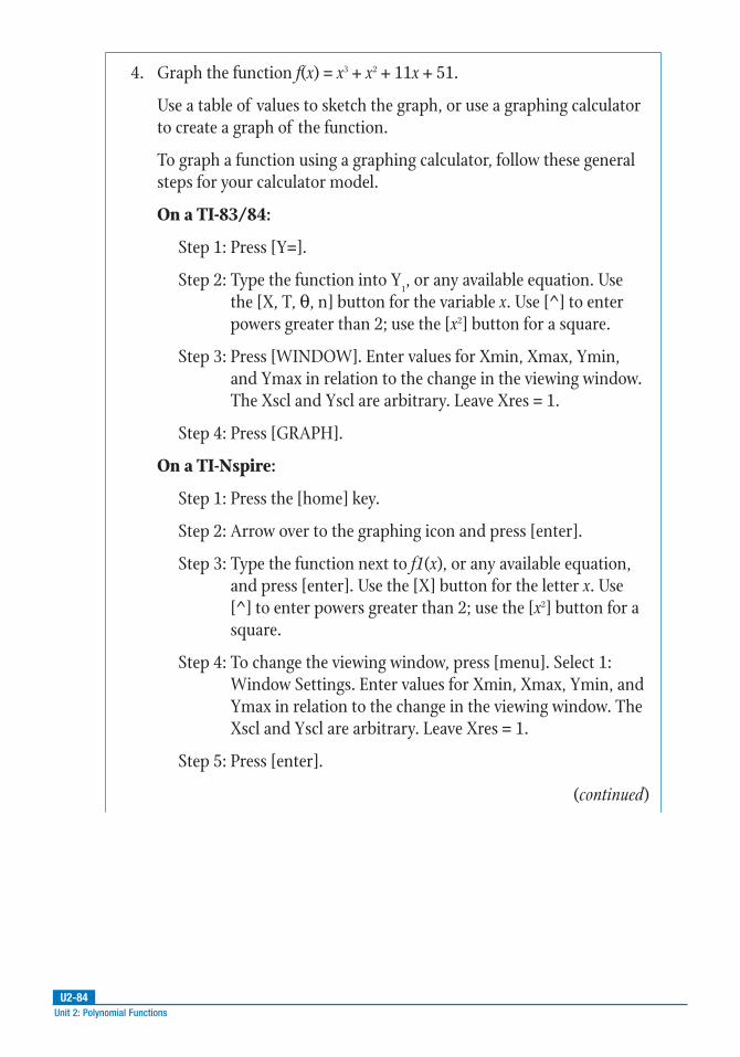
U2-84Unit 2: Polynomial Functions
4. Graph the function f(x) = x3 + x2 + 11x + 51.
Use a table of values to sketch the graph, or use a graphing calculator to create a graph of the function.
To graph a function using a graphing calculator, follow these general steps for your calculator model.
On a TI-83/84:
Step 1: Press [Y=].
Step 2: Type the function into Y1, or any available equation. Use
the [X, T, θ, n] button for the variable x. Use [^] to enter powers greater than 2; use the [x2] button for a square.
Step 3: Press [WINDOW]. Enter values for Xmin, Xmax, Ymin, and Ymax in relation to the change in the viewing window. The Xscl and Yscl are arbitrary. Leave Xres = 1.
Step 4: Press [GRAPH].
On a TI-Nspire:
Step 1: Press the [home] key.
Step 2: Arrow over to the graphing icon and press [enter].
Step 3: Type the function next to f1(x), or any available equation, and press [enter]. Use the [X] button for the letter x. Use [^] to enter powers greater than 2; use the [x2] button for a square.
Step 4: To change the viewing window, press [menu]. Select 1: Window Settings. Enter values for Xmin, Xmax, Ymin, and Ymax in relation to the change in the viewing window. The Xscl and Yscl are arbitrary. Leave Xres = 1.
Step 5: Press [enter].
(continued)

U2-85Lesson 3: Graphing Polynomial Functions
–5 –4 –3 –2 –1 0 1 2 3 4 5
–100
–75
–50
–25
25
50
75
100
125
150
175
200
225
250f(x)
Notice that the graph of the function crosses the x-axis at only one point, (–3, 0). This verifies there is only 1 real root.
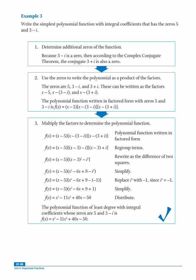
U2-86Unit 2: Polynomial Functions
Example 3
Write the simplest polynomial function with integral coefficients that has the zeros 5 and 3 – i.
1. Determine additional zeros of the function.
Because 3 – i is a zero, then according to the Complex Conjugate Theorem, the conjugate 3 + i is also a zero.
2. Use the zeros to write the polynomial as a product of the factors.
The zeros are 5, 3 – i, and 3 + i. These can be written as the factors x – 5, x – (3 – i), and x – (3 + i).
The polynomial function written in factored form with zeros 5 and 3 – i is f(x) = (x – 5)[x – (3 – i)][x – (3 + i)].
3. Multiply the factors to determine the polynomial function.
f(x) = (x – 5)[x – (3 – i)][x – (3 + i)]Polynomial function written in factored form
f(x) = (x – 5)[(x – 3) – i][(x – 3) + i] Regroup terms.
f(x) = (x – 5)[(x – 3)2 – i2]Rewrite as the difference of two squares.
f(x) = (x – 5)(x2 – 6x + 9 – i2) Simplify.
f(x) = (x – 5)[x2 – 6x + 9 – (–1)] Replace i2 with –1, since i2 = –1.
f(x) = (x – 5)(x2 – 6x + 9 + 1) Simplify.
f(x) = x3 – 11x2 + 40x – 50 Distribute.
The polynomial function of least degree with integral coefficients whose zeros are 5 and 3 – i is f(x) = x3 – 11x2 + 40x – 50.

UNIT 2 • POLYNOMIAL FUNCTIONSLesson 3: Graphing Polynomial Functions
PRACTICE
U2-87Lesson 3: Graphing Polynomial Functions
For problems 1–3, determine the number and type of roots for each equation using one of the given roots. Then find each root.
1. x3 + 4x2 – 4x – 16 = 0; –2
2. x3 – x2 – 5x – 3 = 0; 3
3. x3 – 4x2 + 9x – 10 = 0; 2
For problems 4–6, find all the zeros of each function. Then graph each function to verify your answers.
4. f(x) = x2 + x – 12
5. f(x) = x3 – 13x – 12
6. f(x) = x3 – 8x2 + 22x – 20
For problems 7 and 8, write the simplest polynomial function with integral coefficients that has the given zeros.
7. –3, –2, 1, 5
8. –2, 5 – 2i
Use the following information to solve problems 9 and 10.
An aquarium is in the shape of a rectangular prism. The width of the tank is 4 feet less than its height and its length is 8 feet longer than its height. The volume of the tank is 4,608 cubic inches.
9. What equation represents the volume of the aquarium?
10. Find all the solutions of the polynomial equation. What are the dimensions of the aquarium?
Practice 2.3.3: Finding Zeros

U2-88Unit 2: Polynomial Functions
Lesson 2.3.4:
IntroductionYou have learned several methods for solving polynomial equations by determining the factors, but not all equations are factorable. In this lesson, you will learn how to find the roots of a polynomial equation with integer coefficients that is not factorable.
Key Concepts
• You can find the possible rational roots of a polynomial equation with integer coefficients using the Rational Root Theorem. This theorem states that if a polynomial has rational roots, then those roots will be the ratio of the factors of the constant term to the factors of the leading coefficient written in lowest terms.
• Be sure to include all factors of both the constant term and the leading coefficient, including both the positive and negative factors. It is not necessary to repeat duplicate ratios.
Rational Root TheoremIf the polynomial p(x) has integer coefficients, then every rational root of
the polynomial equation p(x) = 0 can be written in the form p
q, where
p is a factor of the constant term of p(x) and q is a factor of the leading
coefficient of p(x).
• It is possible for polynomial equations to have no rational roots; polynomial equations could also have irrational roots as stated in the Irrational Root Theorem.
Irrational Root Theorem
If a polynomial p(x) has rational coefficients and a b c+ is a root of the polynomial equation p(x) = 0, where a and b are rational and c is irrational, then a b c− is also a root of p(x) = 0.
• Recall that it is also possible for an equation to have imaginary roots in the form a + bi and a – bi, referred to as complex conjugates. If the imaginary number a + bi is a root of a polynomial equation with real coefficients, then the conjugate a – bi is also a root.
Lesson 2.3.4: The Rational Root Theorem

U2-89Lesson 3: Graphing Polynomial Functions
Guided Practice 2.3.4Example 1
Use the Rational Root Theorem to list all the possible rational roots of the polynomial equation 2x4 – 3x3 + 4x2 – 9x + 6 = 0.
1. Identify the constant term and the leading coefficient of the polynomial equation.
The constant term of the polynomial equation is 6.
The polynomial equation is written in descending order; therefore, the leading coefficient comes from the term 2x4. The leading coefficient is 2.
2. Identify the factors of the constant term and the leading coefficient.
The constant, 6, has the factors ±1, ±2, ±3, and ±6.
The leading coefficient, 2, has the factors ±1 and ±2.
3. Identify the possible rational roots of the polynomial equation.
The possible rational roots of the polynomial equation are made up of the ratios of the factors of the constant term and the factors of the leading coefficient.
Use the factors determined in step 2 to set up the ratios.
1, 2, 3, 6
1, 2
± ± ± ±± ±
Ratio of the factors of the constant term and the factors of the leading coefficient
1
1,
1
2,
2
1,
2
2,
3
1,
3
2,
6
1,
6
2
±±
±±
±±
±±
±±
±±
±±
±±
Write a separate ratio for each of the factors.
1,1
2, 2, 1, 3,
3
2, 6, 3± ± ± ± ± ± ± ± Simplify each ratio.
1,1
2, 2, 3,
3
2, 6± ± ± ± ± ± Remove any repeated ratios.
The possible rational roots of the polynomial equation
2x4 – 3x3 + 4x2 – 9x + 6 = 0 are 1,1
2, 2, 3,
3
2, and 6.± ± ± ± ± ±

U2-90Unit 2: Polynomial Functions
Example 2
Find all of the roots to the polynomial equation 4x3 – x2 + 36x – 9 = 0.
1. List all the possible rational roots.
The Rational Root Theorem states that the only possible rational roots of the equation must be ratios of the factors of the constant term and the factors of the leading coefficient.
The constant term is –9 and the leading coefficient is 4.
The factors of the constant term, –9, are ±1, ±3, and ±9.
The factors of the leading coefficient, 4, are ±1, ±2, and ±4.
Use these factors to set up the ratios.
1, 3 9
1, 2, 4
± ± ±± ± ±
Ratio of the factors of the constant term and the factors of the leading coefficient
1
1,
1
2,
1
4,
3
1,
3
2,
3
4,
9
1,
9
2,
9
4
±±
±±
±±
±±
±±
±±
±±
±±
±±
Write a separate ratio for each of the factors.
1,1
2,
1
4, 3,
3
2,
3
4, 9,
9
2,
9
4± ± ± ± ± ± ± ± ± Simplify each ratio.
2. Determine the number of possible roots of the polynomial equation.
4x3 – x2 + 36x – 9 = 0 is a third-degree polynomial.
Therefore, this equation will have either 3 real roots or 1 real root and 2 complex roots.
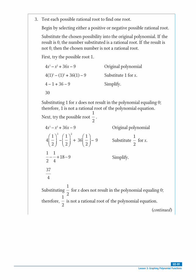
U2-91Lesson 3: Graphing Polynomial Functions
3. Test each possible rational root to find one root.
Begin by selecting either a positive or negative possible rational root.
Substitute the chosen possibility into the original polynomial. If the result is 0, the number substituted is a rational root. If the result is not 0, then the chosen number is not a rational root.
First, try the possible root 1.
4x3 – x2 + 36x – 9 Original polynomial
4(1)3 – (1)2 + 36(1) – 9 Substitute 1 for x.
4 – 1 + 36 – 9 Simplify.
30
Substituting 1 for x does not result in the polynomial equaling 0; therefore, 1 is not a rational root of the polynomial equation.
Next, try the possible root 1
2.
4x3 – x2 + 36x – 9 Original polynomial
41
2–
1
236
1
2– 9
3 2
+
Substitute 1
2 for x.
1
2
1
418 9− + − Simplify.
37
4
Substituting 1
2 for x does not result in the polynomial equaling 0;
therefore, 1
2 is not a rational root of the polynomial equation.
(continued)

U2-92Unit 2: Polynomial Functions
Next, try the possible root 1
4.
4x3 – x2 + 36x – 9 Original polynomial
41
4–
1
436
1
4– 9
3 2
+
Substitute 1
4 for x.
1
16
1
169 9− + − Simplify.
0
Substituting 1
4 for x does result in the polynomial equaling 0;
therefore, 1
4 is a rational root of the polynomial equation.
4. Use synthetic division to find the roots of the depressed polynomial equation.
The divisor is 1
4.
1
44 1 36 9
1 0 9
4 0 36 0
− −
The depressed polynomial is 4x2 + 36.
Find the roots of 4x2 + 36 = 0.
4x2 + 36 = 0 Depressed polynomial
4(x2 + 9) = 0 Factor out the greatest common factor, 4.
x2 + 9 = 0 Divide both sides by 4.
x2 = –9 Subtract 9 from both sides.
9x = − Take the square root of both sides.
9x i= Simplify.
x = ±3i
The roots of the depressed polynomial equation 4x2 + 36 = 0 are ±3i.
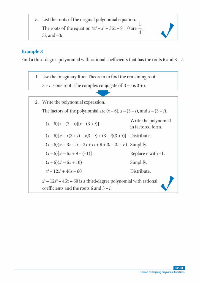
U2-93Lesson 3: Graphing Polynomial Functions
5. List the roots of the original polynomial equation.
The roots of the equation 4x3 – x2 + 36x – 9 = 0 are 1
4,
3i, and –3i.
Example 3
Find a third-degree polynomial with rational coefficients that has the roots 6 and 3 – i.
1. Use the Imaginary Root Theorem to find the remaining root.
3 – i is one root. The complex conjugate of 3 – i is 3 + i.
2. Write the polynomial expression.
The factors of the polynomial are (x – 6), x – (3 – i), and x – (3 + i).
(x – 6)[x – (3 – i)][x – (3 + i)]Write the polynomial in factored form.
(x – 6)[x2 – x(3 + i) – x(3 – i) + (3 – i)(3 + i)] Distribute.
(x – 6)(x2 – 3x – ix – 3x + ix + 9 + 3i – 3i – i2) Simplify.
(x – 6)[x2 – 6x + 9 – (–1)] Replace i2 with –1.
(x – 6)(x2 – 6x + 10) Simplify.
x3 – 12x2 + 46x – 60 Distribute.
x3 – 12x2 + 46x – 60 is a third-degree polynomial with rational coefficients and the roots 6 and 3 – i.
UNIT 2 • POLYNOMIAL FUNCTIONSLesson 3: Graphing Polynomial Functions
PRACTICE
U2-94Unit 2: Polynomial Functions
For problems 1–4, use the Rational Root Theorem to list all of the possible rational roots for each polynomial equation.
1. x3 + 5x2 – 3x + 7 = 0
2. x3 + 3x2 – 8 = 0
3. 6x3 + x2 + 2x + 1 = 0
4. 3x3 + 4x2 – 2x – 18 = 0
For problems 5–8, find all of the roots of each polynomial equation.
5. 2x3 + x2 – 11x – 10 = 0
6. x3 – 3x2 + 2x – 6 = 0
7. x3 – 5x2 + 4x + 6 = 0
8. 4x4 – 13x2 + 7x + 2 = 0
For problems 9 and 10, find a third-degree polynomial with rational coefficients that has the given numbers as roots.
9. 5 and 3
10. –2 and 4 + i
Practice 2.3.4: The Rational Root Theorem

U2-95
Lesson 4: Solving Systems of Equations with Polynomials
UNIT 2 • POLYNOMIAL FUNCTIONS
Lesson 4: Solving Systems of Equations with Polynomials
WORDS TO KNOW
dependent system a system of equations that intersect at every point
empty set a set that has no elements, denoted by ∅; the solution to a system of equations with no intersection points, denoted by { }
independent system a system of equations that have a finite number of points of intersection
linear equation an equation that can be written in the form y = mx + b, in which m is the slope, b is the y-intercept, and the graph is a straight line. The solutions to the linear equation are the infinite set of points on the line.
point(s) of intersection the ordered pair(s) where graphed functions intersect on a coordinate plane; these are also the solutions to systems of equations
polynomial equation an equation of the general form y = anx
n + a
n – 1xn – 1 + …
+ a2x2 + a
1x + a
0, where a
1 is a rational number, a
n ≠ 0,
and n is a nonnegative integer and the highest degree of the polynomial
Essential Questions
1. What is a point of intersection?
2. Can two functions have more than one point of intersection?
3. Do all systems of equations have solutions that are real numbers?
4. How can systems of equations be used to model real-world situations?
Common Core Georgia Performance Standards
MCC9–12.A.REI.7
MCC9–12.A.REI.11★

U2-96Unit 2: Polynomial Functions
quadratic equation an equation that can be written in the form y = ax2 + bx + c, where x is the variable, a, b, and c are constants, and a ≠ 0
quadratic formula a formula that states the solutions of a quadratic
equation of the form ax2 + bx + c = 0 are given by
xb b ac
a
4
2
2
=− ± −
. A quadratic equation in this form
can have no real solutions, one real solution, or two
real solutions.
system of equations a set of equations with the same unknowns
Recommended Resources• MathIsFun.com. “Function Grapher and Calculator.”
http://www.walch.com/rr/00169
This site provides an online graphing utility. Users can enter values to create their own system and then zoom in on the functions to determine approximate intersection points.
• Purplemath.com. “Systems of Non-Linear Equations.”
http://www.walch.com/rr/00170
This site provides a summary of nonlinear systems as well as worked examples.
• Virtual Math Lab. “Solving Systems of Nonlinear Equations in Two Variables.”
http://www.walch.com/rr/00171
This site reviews possible solutions to systems of nonlinear equations. Methods to solve these systems are not limited to graphing.

U2-97Lesson 4: Solving Systems of Equations with Polynomials
Lesson 2.4.1: Solving a Linear-Polynomial System of Equations
IntroductionA system of equations is a set of equations with the same unknowns. It is likely that you have solved a system of equations or a quadratic-linear system in the past. In this lesson, we will learn to solve systems that include at least one polynomial by graphing.
Key Concepts
• The real solutions of a system of equations can often be found by graphing. Recall that the graph of an equation is the set of all the solutions of the equation plotted on a coordinate plane.
• The points of intersection of the graphed system of equations are the ordered pairs where graphed functions intersect on a coordinate plane. These are also the solutions to the system. The solution or solutions to a system of equations with f(x) and g(x) occurs where f(x) = g(x) and the difference between these two values is 0. Also recall that the solutions to a system of equations are written using braces: {}.
• A system may have an infinite number of solutions, a finite number of solutions, or no real solutions.
• A system with a finite number of points of intersection is called an independent system.
• It is possible that a system of equations does not intersect. The solution to such a system of equations is the empty set, denoted by { }.
• A system of equations could also intersect at every point. This type of system is known as a dependent system.

U2-98Unit 2: Polynomial Functions
Solutions to Systems of Equations with Polynomials
–10 –9 –8 –7 –6 –5 –4 –3 –2 –1 0 1 2 3 4 5 6 7 8 9 10
–10
–9
–8
–7
–6
–5
–4
–3
–2
–1
1
2
3
4
5
6
7
8
9
10
f(x) = g(x)
• If the equations overlap, they have an infinite number of solutions.
• This is an example of a dependent system.
–10 –9 –8 –7 –6 –5 –4 –3 –2 –1 0 1 2 3 4 5 6 7 8 9 10
–10
–9
–8
–7
–6
–5
–4
–3
–2
–1
1
2
3
4
5
6
7
8
9
10
g(x)
f(x)
• If the equations intersect, they have a finite number of solutions.
• This is an example of an independent system.
–10 –9 –8 –7 –6 –5 –4 –3 –2 –1 0 1 2 3 4 5 6 7 8 9 10
–10
–9
–8
–7
–6
–5
–4
–3
–2
–1
1
2
3
4
5
6
7
8
9
10
g(x)
f(x)• If the equations do not intersect, they
have no solutions.
• The solution to this system is the empty set.

U2-99Lesson 4: Solving Systems of Equations with Polynomials
• When graphing a system of equations with polynomials, it is helpful to recall various forms of equations and their general shapes.
Graphs of General Equations
Type of equation General equation Graph
Linear equation
m is the slope and b is the y-intercept
y = mx + b
–10 –9 –8 –7 –6 –5 –4 –3 –2 –1 0 1 2 3 4 5 6 7 8 9 10
–10
–9
–8
–7
–6
–5
–4
–3
–2
–1
1
2
3
4
5
6
7
8
9
10
Polynomial equation
a1 is a rational number,
an ≠ 0, and n is a
nonnegative integer and the highest degree of the polynomial
y = anxn + a
n – 1xn – 1 +
… + a2x2 + a
1x + a
0
–10 –9 –8 –7 –6 –5 –4 –3 –2 –1 0 1 2 3 4 5 6 7 8 9 10
–10
–9
–8
–7
–6
–5
–4
–3
–2
–1
1
2
3
4
5
6
7
8
9
10
Quadratic equation
x is the variable, a, b, and c are constants, and a ≠ 0
y = ax2 + bx + c
–10 –9 –8 –7 –6 –5 –4 –3 –2 –1 0 1 2 3 4 5 6 7 8 9 10
–10
–9
–8
–7
–6
–5
–4
–3
–2
–1
1
2
3
4
5
6
7
8
9
10

U2-100Unit 2: Polynomial Functions
• To graph a system of equations, create a table of values and plot each coordinate on the same coordinate plane. It may be necessary to find additional points to determine where the point(s) of intersection may occur. Each point of intersection represents a solution to the system.
• Solutions to a system of equations can also be identified in a table by finding points such that the y-value of each function is the same for a particular x-value.
• Using a graphing calculator to graph both equations is often helpful. Most calculators have a trace feature to approximate where the equations intersect, or can display a table of values for each equation so you can analyze the values. Some calculators will find intersection points for you.
• To confirm a solution to a system, substitute the coordinates for x and y in both of the original equations. If the intersection point is approximated, the results will be nearly equal.
Solving Systems of Equations Algebraically
• When solving a quadratic-linear system, if both functions are written in the form of a function (such as “y =” or “f(x) =”), set the equations equal to each other.
• When you set the equations equal to each other, you are replacing y in each equation with an equivalent expression, thus using the substitution method to find a solution.
• Recall that you can then solve by factoring the equation or by using the
quadratic formula. The quadratic formula states that the solutions of a
quadratic equation of the form ax2 + bx + c = 0 are given by xb b ac
a
4
2
2
=− ± −
.
A quadratic equation in this form can have no real solutions, one real solution, or
two real solutions.

U2-101Lesson 4: Solving Systems of Equations with Polynomials
Example 1
Use the graph to estimate the solution(s), if any, to the system of equations.
–7 –6 –5 –4 –3 –2 –1 0 1 2 3 4 5 6 7
–80
–70
–60
–50
–40
–30
–20
–10
10
20
30
40
50
60
f(x)
g(x)
1. Determine the number of times the graphs of f(x) and g(x) intersect.
The graphs of f(x) and g(x) appear to intersect at three points.
2. Estimate the points of intersection.
The scale of the graph provided determines how accurately the solution can be approximated. It appears as though the graphs intersect at approximately (–3, –70), (0.4, –4), and (3, 50). It is not possible to more accurately approximate this solution, as the original equations are not provided.
The approximate solution to this system of equations is {(–3, –70), (0.4, –4), (3, 50)}.
Guided Practice 2.4.1

U2-102Unit 2: Polynomial Functions
Example 2Use a graph to estimate the real solution(s), if any, to the system of equations
( ) 4 1
( ) 13
= +
= +
f x x
g x x. Verify that any identified coordinate pairs are solutions.
1. Create a graph of the two functions, f(x) and g(x).
You can use what you have learned about graphing equations to graph each equation on the same coordinate plane, or you can use a graphing calculator.
To graph the system on your graphing calculator, follow the directions appropriate to your calculator model.
On a TI-83/84:
Step 1: Press the [Y=] button.
Step 2: Type the first function into Y1, using the [X, T, θ, n] button
for the variable x. Press [ENTER].
Step 3: Type the second function into Y2, using the [^] button for
powers. Press [ENTER].
Step 4: Press [ZOOM]. Arrow down to 6: ZStandard. Press [ENTER].
On a TI-Nspire:
Step 1: Press the [home] key.
Step 2: Arrow over to the graphing icon and press [enter].
Step 3: Type the first function next to f1(x), using the [X] button for the letter x or the [x2] button for a square. Press [enter].
Step 4: To graph the second function, press [menu] and arrow down to 3: Graph Type. Arrow right to bring up the sub-menu, then select 1: Function. Press [enter].
Step 5: At f2(x), type the second function and press [enter].
Step 6: To change the viewing window, press [menu]. Select 4: Window/Zoom and select A: Zoom – Fit.
(continued)
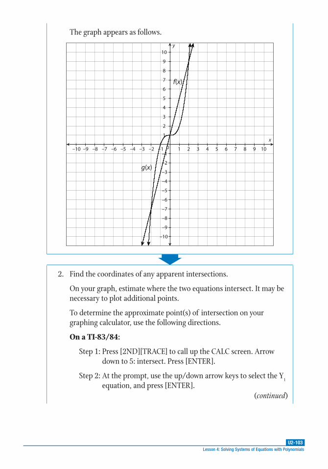
U2-103Lesson 4: Solving Systems of Equations with Polynomials
The graph appears as follows.
–10 –9 –8 –7 –6 –5 –4 –3 –2 –1 0 1 2 3 4 5 6 7 8 9 10
–10
–9
–8
–7
–6
–5
–4
–3
–2
–1
1
2
3
4
5
6
7
8
9
10
f(x)
g(x)
2. Find the coordinates of any apparent intersections.
On your graph, estimate where the two equations intersect. It may be necessary to plot additional points.
To determine the approximate point(s) of intersection on your graphing calculator, use the following directions.
On a TI-83/84:
Step 1: Press [2ND][TRACE] to call up the CALC screen. Arrow down to 5: intersect. Press [ENTER].
Step 2: At the prompt, use the up/down arrow keys to select the Y1
equation, and press [ENTER].(continued)
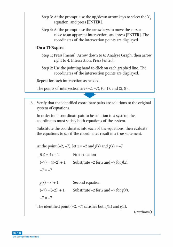
U2-104Unit 2: Polynomial Functions
Step 3: At the prompt, use the up/down arrow keys to select the Y2
equation, and press [ENTER].
Step 4: At the prompt, use the arrow keys to move the cursor close to an apparent intersection, and press [ENTER]. The coordinates of the intersection points are displayed.
On a TI-Nspire:
Step 1: Press [menu]. Arrow down to 6: Analyze Graph, then arrow right to 4: Intersection. Press [enter].
Step 2: Use the pointing hand to click on each graphed line. The coordinates of the intersection points are displayed.
Repeat for each intersection as needed.
The points of intersection are (–2, –7), (0, 1), and (2, 9).
3. Verify that the identified coordinate pairs are solutions to the original system of equations.
In order for a coordinate pair to be solution to a system, the coordinates must satisfy both equations of the system.
Substitute the coordinates into each of the equations, then evaluate the equations to see if the coordinates result in a true statement.
At the point (–2, –7), let x = –2 and f(x) and g(x) = –7.
f(x) = 4x + 1 First equation
(–7) = 4(–2) + 1 Substitute –2 for x and –7 for f(x).
–7 = –7
g(x) = x3 + 1 Second equation
(–7) = (–2)3 + 1 Substitute –2 for x and –7 for g(x).
–7 = –7
The identified point (–2, –7) satisfies both f(x) and g(x).(continued)

U2-105Lesson 4: Solving Systems of Equations with Polynomials
At the point (0, 1), let x = 0 and f(x) and g(x) = 1.
f(x) = 4x + 1 First equation
(1) = 4(0) + 1 Substitute 0 for x and 1 for f(x).
1 = 1
g(x) = x3 + 1 Second equation
(1) = (0)3 + 1 Substitute 0 for x and 1 for g(x).
1 = 1
The identified point (0, 1) satisfies both f(x) and g(x).
At the point (2, 9), let x = 2 and f(x) and g(x) = 9.
f(x) = 4x + 1 First equation
(9) = 4(2) + 1 Substitute 2 for x and 9 for f(x).
9 = 9
g(x) = x3 + 1 Second equation
(9) = (2)3 + 1 Substitute 2 for x and 9 for g(x).
9 = 9
The identified point (2, 9) satisfies both f(x) and g(x).
The solution set to the system of equations ( ) 4 1
( ) 13
= +
= +
f x x
g x x
is {(–2, –7), (0, 1), (2, 9)}, as identified on the graph as the
intersections of the lines f(x) and g(x).

U2-106Unit 2: Polynomial Functions
Example 3Create a table to approximate the real solution(s), if any, to the system
f x x
g x x x
( )1
2
3
2( ) 3 14 3
=− −
= + +
.
1. Create a table of values for the two functions f(x) and g(x).
You can create a table of values by hand similarly to how you have created them in the past, or you can use your graphing calculator.
To create a table of values using your graphing calculator, follow the directions appropriate to your calculator model.
On a TI-83/84:
Step 1: Press the [Y=] button. Clear any equations from previous calculations.
Step 2: Type the first function into Y1, using the [X, T, θ, n] button
for the variable x. Press [ENTER].
Step 3: Type the second function into Y2. Use the [^] button for
powers. After entering a power, press the right arrow button to get out of exponent mode. Press [ENTER].
Step 4: Press [2ND][WINDOW] to call up the TABLE SETUP screen. Set TblStart to –5 by clearing out any current values and typing [(–)][5][ENTER]. Set ∆Tbl to 1, then press [2ND][GRAPH] to call up the TABLE screen. A table of values for both equations will be displayed.
On a TI-Nspire:
Step 1: Press the [home] key.
Step 2: Arrow over to the calculator page, the first icon over, and press [enter].
Step 3: Define f(x) by entering “define” and then the function using the buttons on your keypad. Remember to enter a space after “define”. Press [enter].
(continued)

U2-107Lesson 4: Solving Systems of Equations with Polynomials
Step 4: Define g(x) by entering “define” and then the function using the buttons on your keypad. Remember to press the right arrow key after entering an exponent. Press [enter].
Step 5: Press the [home] key. Arrow over to the spreadsheets page, the fourth icon over, and press [enter].
Step 6: Press [ctrl][T] to switch to a table window. From the list of defined functions that appears, select f(x)f1, and press [enter].
Step 7: Press the right arrow key. From the list of defined functions that appears, select f(x)g1, and press [enter]. A table of values for both equations will be displayed.
Both calculators should yield a table that resembles the following.
x –5 –4 –3 –2 –1 0 1 2 3f(x) 1 0.5 0 –0.5 –1 –1.5 –2 –2.5 –3g(x) 251 65 1 –7 –1 1 5 41 163
2. Estimate the points of intersection.
Compare the y-values for the same x-value in your completed table.
Look for places where the difference between the values for g(x) and f(x) is decreasing. If the difference between g(x) and f(x) is increasing, then any intersection occurs in the other direction. The point of intersection occurs when f(x) is equal to g(x) or the difference is 0.
x –5 –4 –3 –2 –1 0 1 2 3f(x) 1 0.5 0 –0.5 –1 –1.5 –2 –2.5 –3g(x) 251 65 1 –7 –1 1 5 41 163g(x) – f(x) +250 +64.5 +1 –6.5 0 +2.5 +7 +43.5 +166
Notice that in the table, f(x) equals g(x) when x = –1. Also notice that there appears to be a second intersection point close to the x-values of –3 and –2.
To better approximate the second point of intersection, you must find additional values.
Use the following directions to determine additional values on your graphing calculator.
(continued)

U2-108Unit 2: Polynomial Functions
On a TI-83/84:
Step 1: Press [2ND][WINDOW] to call up the TABLE SETUP screen. Set the TblStart to –3 and ∆Tbl to 0.01, clearing out any previous values. Press [ENTER], then press [2ND][GRAPH] to call up the TABLE screen. A table of values for both equations will be displayed.
Step 2: Scroll through the table of values to determine the approximate solutions.
On a TI-Nspire:
Step 1: Press [menu]. Use the arrow keys to select 5: Table, then 5: Edit Table Settings. Set the Table Start to –3 and Table Step to 0.01. Arrow down to OK and press [enter]. You may need to readjust the Table Step setting to get a better approximation of when f(x) = g(x).
The following table displays information for values of x close to the point we’re interested in: x = –3.
x –3.00 –2.99 –2.98 –2.97 –2.96 –2.95 –2.94 –2.93
f(x) 0 –0.005 –0.010 –0.015 –0.020 –0.025 –0.030 –0.035
g(x) 1 0.7327 0.4707 0.2141 –0.0374 –0.2836 –0.5247 –0.7608
g(x) – f(x) +1 +0.7377 +0.4807 +0.2291 –0.0174 –0.2586 –0.4947 –0.7258
Since we know that the difference between g(x) and f(x) is smallest for values of x close to –3, review the table near this value. Determine where the values of g(x) and f(x) have the smallest difference.
According to the generated table of additional values, the value of x with the smallest difference between g(x) and f(x) is –2.96. Because the difference in values is so small and because the coordinates are approximate, it is appropriate to use either the f(x) value or the g(x) value when stating the solution.
It can be seen from the tables that –1 and the approximate value of –2.96 are the x-coordinates at which f(x) and g(x) intersect; therefore, the approximate solutions to the system are (–2.96, –0.02) and (–1, –1).

U2-109Lesson 4: Solving Systems of Equations with Polynomials
3. Verify that the identified coordinates are solutions to the original system of equations.
In order for a coordinate to be a solution to a system, the coordinate must satisfy both equations of the system. Because our coordinates are estimated, it is quite possible that our results will be nearly equal, but not exactly equal.
Substitute the coordinates into each of the equations, then evaluate the equations to see if the coordinates result in a true statement.
At the point (–2.96, –0.02), let x = –2.96 and f(x) and g(x) = –0.02.
f x x( )1
2
3
2=− − First equation
( 0.02)1
2( 2.96)
3
2− =− − − Substitute –2.96 for x and –0.02
for f(x).
–0.02 = –0.02
g(x) = x4 + 3x3 + 1 Second equation
(–0.02) = (–2.96)4 + 3(–2.96)3 + 1 Substitute –2.96 for x and –0.02 for g(x).
–0.02 ≈ –0.04
The identified point (–2.96, –0.02) nearly satisfies both f(x) and g(x), and can be considered an approximate solution to the system of equations.
At the point (–1, –1), let x = –1 and f(x) and g(x) = –1.
f x x( )1
2
3
2=− − First equation
( 1)1
2( 1)
3
2− =− − − Substitute –1 for x and –1 for f(x).
–1 = –1(continued)

U2-110Unit 2: Polynomial Functions
g(x) = x4 + 3x3 + 1 Second equation
(–1) = (–1)4 + 3(–1)3 + 1 Substitute –1 for x and –1 for g(x).
–1 = –1
The identified point (–1, –1) satisfies both f(x) and g(x), and is a solution to the system of equations.
The approximate solution set to the system f x x
g x x x
( )1
2
3
2( ) 3 14 3
=− −
= + +
is
{(–2.96, –0.02), (–1, –1)}, as identified in the tables as the intersection
of the equations f(x) and g(x).
Graphing the system shows that our approximated solution set is valid.
–10 –9 –8 –7 –6 –5 –4 –3 –2 –1 0 1 2 3 4 5 6 7 8 9 10
–10
–9
–8
–7
–6
–5
–4
–3
–2
–1
1
2
3
4
5
6
7
8
9
10
g(x)
f(x)
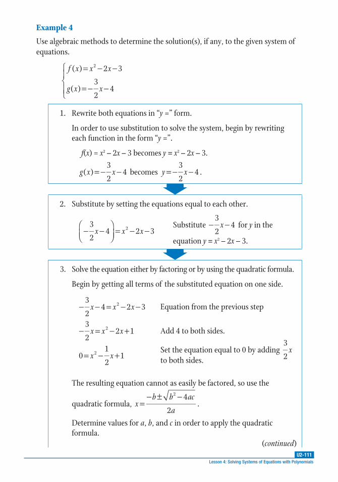
U2-111Lesson 4: Solving Systems of Equations with Polynomials
Example 4
Use algebraic methods to determine the solution(s), if any, to the given system of equations.
f x x x
g x x
( ) 2 3
( )3
24
2= − −
=− −
1. Rewrite both equations in “y =” form.
In order to use substitution to solve the system, begin by rewriting each function in the form “y =”.
f(x) = x2 – 2x – 3 becomes y = x2 – 2x – 3.
g x x( )3
24=− − becomes y x
3
24=− − .
2. Substitute by setting the equations equal to each other.
x x x− −
= − −
3
24 2 32 Substitute x
3
24− − for y in the
equation y = x2 – 2x – 3.
3. Solve the equation either by factoring or by using the quadratic formula.
Begin by getting all terms of the substituted equation on one side.
x x x3
24 2 32− − = − − Equation from the previous step
x x x3
22 12− = − + Add 4 to both sides.
x x01
212= − +
Set the equation equal to 0 by adding x3
2
to both sides.
The resulting equation cannot as easily be factored, so use the
quadratic formula, xb b ac
a
4
2
2
=− ± −
.
Determine values for a, b, and c in order to apply the quadratic formula.
(continued)

U2-112Unit 2: Polynomial Functions
For the equation x x01
212= − + , a = 1, b =
1
2− , and c = 1.
x x01
212= − + Equation set equal to 0
x
1
2
1
24 1 1
2 1
2
( )( )
( )=− −
± −
− Substitute values for a, b, and c
into the quadratic formula.
x
1
2
1
44
2=
± −
Simplify.
x
1
2
15
42
=± −
Since the value under the square root is negative, there are no real solutions to the quadratic. Simplify to find the complex solutions. Remember that i 1= − .
x
1
2
15
42
=± − Previous equation
x1
2
15
4
1
2= ± −
• Rewrite the fraction as a product of
two fractions.
x1
2
1
2
15
4
1
2=
± −
Distribute.
x1
4
15
4
1
2=
±
−
Simplify the first product and rewrite the fraction under the square root as a fraction of two square roots.
x1
4
15
2
1
2=
±
−
Simplify the square root in the denominator.
x1
4
15
4=
±
−
Simplify the second product.
xi1 15
4=
±Simplify.

U2-113Lesson 4: Solving Systems of Equations with Polynomials
4. Check your results by graphing.
Graph by hand, or follow the graphing calculator steps outlined in Example 2.
–10 –9 –8 –7 –6 –5 –4 –3 –2 –1 0 1 2 3 4 5 6 7 8 9 10
–10
–9
–8
–7
–6
–5
–4
–3
–2
–1
1
2
3
4
5
6
7
8
9
10
f(x)
g(x)
The graph confirms our algebraically determined conclusion that the system has no solutions.
The system f x x x
g x x
( ) 2 3
( )3
24
2= − −
=− −
has no real solutions, but the
complex solutions are when xi1 15
4=
±.
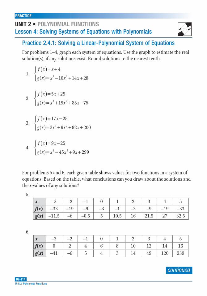
UNIT 2 • POLYNOMIAL FUNCTIONSLesson 4: Solving Systems of Equations with Polynomials
PRACTICE
U2-114Unit 2: Polynomial Functions
For problems 1–4, graph each system of equations. Use the graph to estimate the real solution(s), if any solutions exist. Round solutions to the nearest tenth.
1. f x x
g x x x x
4
( ) 10 14 283 2
( )= +
= − + +
2. f x x
g x x x x
5 25
( ) 19 85 753 2
( )= +
= + + −
3. f x x
g x x x x
17 25
( ) 3 9 92 2003 2
( )= −
= + + +
4. f x x
g x x x x
9 25
( ) 45 9 2994 2
( )= −
= − + +
For problems 5 and 6, each given table shows values for two functions in a system of equations. Based on the table, what conclusions can you draw about the solutions and the x-values of any solutions?
5. x –3 –2 –1 0 1 2 3 4 5f(x) –33 –19 –9 –3 –1 –3 –9 –19 –33g(x) –11.5 –6 –0.5 5 10.5 16 21.5 27 32.5
6. x –3 –2 –1 0 1 2 3 4 5f(x) 0 2 4 6 8 10 12 14 16g(x) –41 –6 5 4 3 14 49 120 239
Practice 2.4.1: Solving a Linear-Polynomial System of Equations
continued
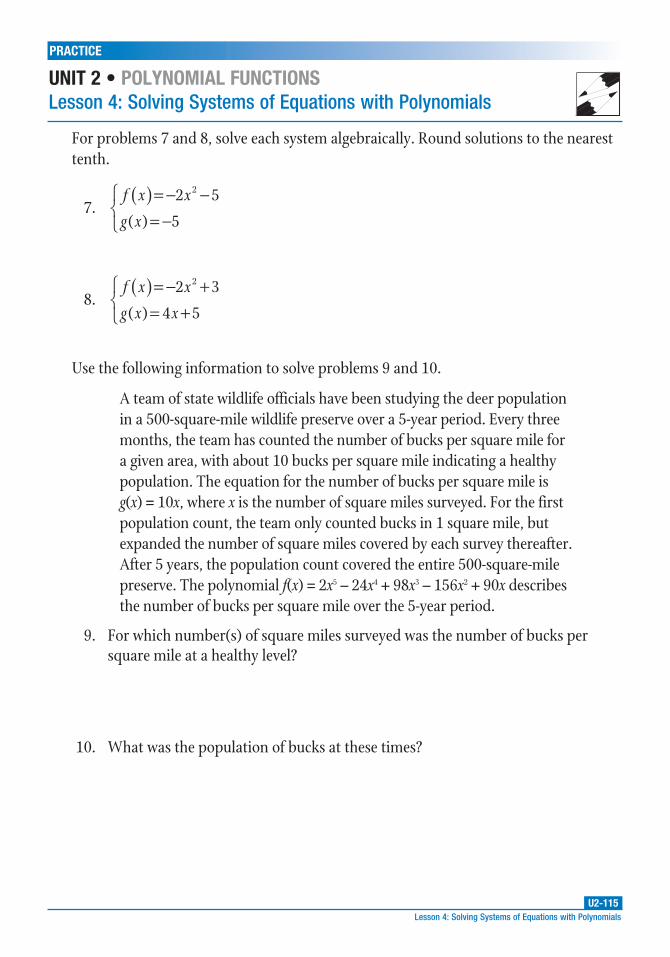
UNIT 2 • POLYNOMIAL FUNCTIONSLesson 4: Solving Systems of Equations with Polynomials
PRACTICE
U2-115Lesson 4: Solving Systems of Equations with Polynomials
For problems 7 and 8, solve each system algebraically. Round solutions to the nearest tenth.
7. f x x
g x
2 5
( ) 5
2( )= − −=−
8. f x x
g x x
2 3
( ) 4 5
2( )= − += +
Use the following information to solve problems 9 and 10.
A team of state wildlife officials have been studying the deer population in a 500-square-mile wildlife preserve over a 5-year period. Every three months, the team has counted the number of bucks per square mile for a given area, with about 10 bucks per square mile indicating a healthy population. The equation for the number of bucks per square mile is g(x) = 10x, where x is the number of square miles surveyed. For the first population count, the team only counted bucks in 1 square mile, but expanded the number of square miles covered by each survey thereafter. After 5 years, the population count covered the entire 500-square-mile preserve. The polynomial f(x) = 2x5 – 24x4 + 98x3 – 156x2 + 90x describes the number of bucks per square mile over the 5-year period.
9. For which number(s) of square miles surveyed was the number of bucks per square mile at a healthy level?
10. What was the population of bucks at these times?
U2-116
Lesson 5: Geometric SeriesUNIT 2 • POLYNOMIAL FUNCTIONS
Unit 2: Polynomial Functions
Common Core Georgia Performance Standard
MCC9–12.A.SSE.4★
Essential Questions
1. What is a geometric sequence?
2. How are geometric sequences related to geometric series?
3. How are geometric series used in the real world?
WORDS TO KNOW
common ratio the ratio of a term in a geometric sequence to the
previous term in that sequence; indicated by the
variable r and given by the formula 1
ra
an
n
=−
converge to approach a finite limit. If the sequence of the partial sums of a series approaches the value of a given number (the limit), then the entire series converges to that limit; that is, the series has a sum. An infinite series converges when the absolute value of the common ratio r is less than 1 1r( )< .
discrete function a function in which every element of the domain is individually separate and distinct; a geometric sequence is a discrete function
diverge to not approach a finite limit. If a series does not have a sum (that is, the sequence of its partial sums does not approach a given number), then the series diverges. An infinite series diverges when the absolute value of the common ratio r is greater than 1 1r( )> .
U2-117Lesson 5: Geometric Series
explicit formula for a geometric sequence
a formula used to find any term in a sequence. The formula is a
n = a
1 • r n – 1, where n is a positive integer
that represents the number of terms in the sequence, r is the common ratio, a
1 is the value of the first term
in the sequence, and an is the value of the nth term of
the sequence.
finite limited in number
finite geometric series a series that has a limited or definite number of terms;
can be written as 11
1
a r k
k
n
∑ −
=
, where n is a positive
integer that represents the number of terms in the
series, a1 is the first term, r is the common ratio, and k
is the number of the term
geometric sequence an ordered list of terms in which each new term is the product of the preceding term and a common ratio, r. For a sequence to be geometric, r cannot be equal to 1 (r ≠ 1).
geometric series the sum of a specified number of terms from a geometric sequence
infinite having no limit; represented by the infinity symbol, ∞
infinite geometric series a series that has an unlimited number of terms n( )=∞ ;
can be written as 11
1
a r k
k∑ −
=
∞
, where a1 is the first term, r is
the common ratio, and k is the number of the term
partial sum the sum of part of a series
recursive formula for a geometric sequence
a formula used to find the next term in a sequence. The formula is a
n = a
n – 1 • r, where n is a positive integer that
represents the number of terms in the sequence and r is the common ratio.
sequence an ordered list of numbers or elements
series the sum of the terms of a sequence
sigma (uppercase), ∑ a Greek letter used to represent the summation of values

U2-118Unit 2: Polynomial Functions
sum formula for a finite geometric series
(1 )
11S
a r
rn
n
=−−
, where Sn is the sum, a
1 is the first term,
r is the common ratio, and n is the number of terms
sum formula for an infinite geometric series 1
1Sa
rn = −, where S
n is the sum, a
1 is the first term, and r
is the common ratio
summation notation a symbolic way to represent a series (the sum of a sequence) using the uppercase Greek letter sigma, ∑
term an element in a sequence. In the sequence {a
1, a
2, a
3, …, a
n}, a
1 is the first term, a
2 is the second
term, a3 is the third term, and a
n is the nth term.
Recommended Resources• Amortization-Calc.com. “Amortization Schedule Calculator.”
http://www.walch.com/rr/00172
This site shows a real-world example of sums of finite series. Users can see exactly how much they can expect to pay for a home when taking out a mortgage. Enter values for the loan amount, number of years, interest rate, ZIP code, and the starting month of the loan, then click “Calculate.” The next screen reveals the monthly payment, the total amount paid over the life of the loan, the total amount of interest paid, and the pay-off date.
• Gries, Dan. “Fractal Maker.”
http://www.walch.com/rr/00173
Users of this applet can draw fractals by choosing a number of line segments and manipulating the points on the line. Clicking the “go” button shows the result of the fractal generated following four steps of the self-similar shape the user creates. The applet also allows users to see the progression by choosing which steps will display on the canvas.
U2-119Lesson 5: Geometric Series
• Interactivate. “Sequencer.”
http://www.walch.com/rr/00174
This site allows the user to generate a sequence and graph. Users enter a starting value, a multiplier, and a number of steps for the sequence. Clicking “Calculate Sequence” reveals the numbers in the sequence, along with a graph displaying the value of each term at each numbered step in the sequence.
• NRICH: Enriching Mathematics. “Proof Sorter—Geometric Series.”
http://www.walch.com/rr/00175
On this site, users are shown the steps of the proof for the sum formula for a geometric series, but out of order. Users must rearrange the steps in the correct order; drag a step to the “Spare” space to free up some room before starting. The graphic on the left-hand side of the page moves with each rearrangement of the steps. Each correctly placed step moves the graphic toward 1; incorrectly placed steps move the graphic toward –1.
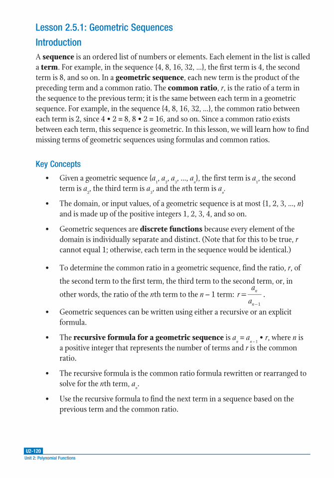
U2-120Unit 2: Polynomial Functions
IntroductionA sequence is an ordered list of numbers or elements. Each element in the list is called a term. For example, in the sequence {4, 8, 16, 32, …}, the first term is 4, the second term is 8, and so on. In a geometric sequence, each new term is the product of the preceding term and a common ratio. The common ratio, r, is the ratio of a term in the sequence to the previous term; it is the same between each term in a geometric sequence. For example, in the sequence {4, 8, 16, 32, …}, the common ratio between each term is 2, since 4 • 2 = 8, 8 • 2 = 16, and so on. Since a common ratio exists between each term, this sequence is geometric. In this lesson, we will learn how to find missing terms of geometric sequences using formulas and common ratios.
Key Concepts
• Given a geometric sequence {a1, a
2, a
3, …, a
n}, the first term is a
1, the second
term is a2, the third term is a
3, and the nth term is a
n.
• The domain, or input values, of a geometric sequence is at most {1, 2, 3, …, n} and is made up of the positive integers 1, 2, 3, 4, and so on.
• Geometric sequences are discrete functions because every element of the domain is individually separate and distinct. (Note that for this to be true, r cannot equal 1; otherwise, each term in the sequence would be identical.)
• To determine the common ratio in a geometric sequence, find the ratio, r, of
the second term to the first term, the third term to the second term, or, in
other words, the ratio of the nth term to the n – 1 term: 1
ra
an
n
=−
.
• Geometric sequences can be written using either a recursive or an explicit formula.
• The recursive formula for a geometric sequence is an = a
n – 1 • r, where n is
a positive integer that represents the number of terms and r is the common ratio.
• The recursive formula is the common ratio formula rewritten or rearranged to solve for the nth term, a
n.
• Use the recursive formula to find the next term in a sequence based on the previous term and the common ratio.
Lesson 2.5.1: Geometric Sequences

U2-121Lesson 5: Geometric Series
• The explicit formula for a geometric sequence is an = a
1 • r n – 1, where n is a
positive integer that represents the number of terms, r is the common ratio, a1
is the value of the first term in the sequence, and an is the value of the nth term
of the sequence.
• Use the explicit formula to find the nth term of a sequence when the first term and common ratio are known.
• The table that follows compares the terms in these two formulas.
Recursive Formula Versus Explicit Formula
Term number (n) 1 2 3 4 … n
Recursive term a1
a1 • r a
2 • r a
3 • r … a
n – 1 • r
Explicit term a1 • r0 a
1 • r1 a
1 • r2 a
1 • r3 … a
1 • r n – 1

U2-122Unit 2: Polynomial Functions
Example 1
Find the missing terms in the sequence that follows.
{1.2, 3.6, 10.8, 32.4, a5, a
6, a
7, …}
1. Determine whether there exists in the sequence a common ratio, r.
The common ratio is determined using the formula 1
ra
an
n
=−
.
Start by labeling each known term of the sequence in the format an
(a1 = 1.2, etc.). Then substitute pairs of terms into the common ratio
formula to determine whether a common ratio exists among the pairs.
a1 = 1.2, a
2 = 3.6, a
3 = 10.8, a
4 = 32.4 Label the known terms as a
1, etc.
Determine the ratio between the first pair of numbers in the sequence.
3.6
1.231
2
1
ra
a
( )( )= = =
Let the numerator be a2 and the
denominator be a1. Substitute
values, then evaluate.Determine the ratio between the second pair of numbers in the sequence.
10.8
3.632
3
2
ra
a
( )( )= = =
Let the numerator be a3 and the
denominator be a2. Substitute
values, then evaluate.Determine the ratio between the third pair of numbers in the sequence.
32.4
10.833
4
3
ra
a
( )( )= = =
Let the numerator be a4 and the
denominator be a3. Substitute
values, then evaluate.Compare the ratios.
Since 32
1
3
2
4
3
a
a
a
a
a
a= = = , the ratios are common and the common ratio,
r, is 3. A common ratio exists, so the sequence is geometric.
Guided Practice 2.5.1

U2-123Lesson 5: Geometric Series
2. Use the common ratio and the fourth term to find the next term in the sequence.
The term we need to find is the fifth term, a5.
Since this is a geometric sequence, the recursive formula can be used to calculate the fifth term. That is, the previous term can be multiplied by the common ratio to calculate the next term. Therefore, multiply a
4
by the common ratio to obtain the fifth term, a5.
We are given that a4 = 32.4.
We have already determined the common ratio, r = 3.
Set up the equation and evaluate.
a5 = a
4 • r Recursive formula to find the fifth term
a5 = (32.4) • (3) Substitute known values.
a5 = 97.2 Multiply to obtain the next term in the sequence.
The fifth term, a5, is 97.2.
3. Use the common ratio and the fifth term to find the next term in the sequence.
The next term we need to find is the sixth term, a6.
Use the recursive formula to multiply a5 by the common ratio to
obtain the sixth term, a6.
From the previous step, we know that a5 = 97.2.
We have already determined the common ratio, r = 3.
Set up the equation and evaluate.
a6 = a
5 • r Recursive formula to find the sixth term
a6 = (97.2) • (3) Substitute known values.
a6 = 291.6 Multiply to obtain the next term in the sequence.
The sixth term, a6, is 291.6.

U2-124Unit 2: Polynomial Functions
4. Use the common ratio and the sixth term to find the next term in the sequence.
The next term we need to find is the seventh term, a7.
Use the recursive formula to multiply a6 by the common ratio to
obtain the seventh term, a7.
From the previous step, we know that a6 = 291.6.
We have already determined the common ratio, r = 3.
Set up the equation and evaluate.
a7 = a
6 • r Recursive formula to find the seventh term
a7 = (291.6) • (3) Substitute known values.
a7
= 874.8 Multiply to obtain the next term in the sequence.
The seventh term, a7, is 874.8.
5. Summarize your results.
Write the first seven terms of the sequence.
Terms of a sequence are written inside a set of braces {}, separated by commas and followed by an ellipsis (…) to show that the sequence continues.
{1.2, 3.6, 10.8, 32.4, 97.2, 291.6, 874.8, …}

U2-125Lesson 5: Geometric Series
Example 2
Find the specified term, an, given the first term and the common ratio.
a1 = 128,
1
2r = , n = 8
1. Determine which geometric sequence formula to use: the recursive formula or the explicit formula.
Since we are given the first term, use the explicit formula.
an = a
1 • r n – 1
2. Use this formula and the given information to find the value of the given term.
We are given that a1 = 128 and
1
2r = .
an = a
1 • r n – 1 Explicit formula
a ( )= •
−
1281
2(8)
(8) 1
Substitute 128 for a1,
1
2 for r, and 8 for n.
1281
28
7
a = •
Simplify the exponent.
a8 = 128 • 0.0078125 Apply the exponent.
a8 = 1 Multiply.
The eighth term of the sequence, a8, is 1.

U2-126Unit 2: Polynomial Functions
Example 3
Write the recursive formula for the geometric sequence that follows, then determine the missing terms in the sequence.
{0.32, 0.48, 0.72, 1.08, a5, a
6, a
7, …}
1. Determine the common ratio, r.
The common ratio is determined using the formula 1
ra
an
n
=−
.
Label the known terms of the sequence in the format an.
a1 = 0.32, a
2 = 0.48, a
3 = 0.72, a
4 = 1.08
Substitute pairs of known terms into the common ratio formula, then evaluate to find the ratio for each pair.
0.48
0.321.51
2
1
ra
a
( )( )= = =
0.72
0.481.52
3
2
ra
a
( )( )= = =
1.08
0.721.53
4
3
ra
a
( )( )= = =
Compare the ratios.
Since 1.52
1
3
2
4
3
a
a
a
a
a
a= = = , the ratios are common and the common
ratio, r, is 1.5.

U2-127Lesson 5: Geometric Series
2. Write the recursive formula for the nth term.
Since the previous terms are known and we are extending the sequence, determine the recursive formula for the sequence.
The recursive formula is the ratio formula, 1
ra
an
n
=−
, rewritten to solve for a
n.
Rewrite the common ratio formula, then substitute known information to find the recursive formula for this sequence.
1
ra
an
n
=−
Common ratio formula
r • an – 1
= an
Multiply both sides by an – 1
.
an = r • a
n – 1
Use the symmetric property of equality to rearrange the equation so that a
n is on the left side.
an = (1.5) • a
n – 1Substitute 1.5 for r.
The recursive formula for the nth term of this sequence is a
n = 1.5 • a
n – 1.
3. Use the recursive formula and the known information to calculate the missing terms in the sequence.
The first four terms are given:
a1 = 0.32, a
2 = 0.48, a
3 = 0.72, a
4 = 1.08
To determine the next term in the sequence, use the fourth term, a4,
to find the fifth term, a5.
We are given that a4 = 1.08.
an = 1.5 • a
n – 1Recursive formula for the given sequence
a(5)
= 1.5 • a(5) – 1
Substitute 5 for n.
a5 = 1.5 • a
4Simplify.
a5 = 1.5 • (1.08) Substitute 1.08 for a
4.
a5 = 1.62 Simplify.
The fifth term, a5, is 1.62.
(continued)

U2-128Unit 2: Polynomial Functions
Since we now know a5 = 1.62, use this information to find the sixth
term, a6.
an = 1.5 • a
n – 1Recursive formula for the given sequence
a(6)
= 1.5 • a(6) – 1
Substitute 6 for n.
a6 = 1.5 • a
5Simplify.
a6 = 1.5 • (1.62) Substitute 1.62 for a
5.
a6 = 2.43 Simplify.
The sixth term, a6, is 2.43.
Since we now know a6 = 2.43, use this information to find the seventh
term, a7.
an = 1.5 • a
n – 1Recursive formula for the given sequence
a(7)
= 1.5 • a(7) – 1
Substitute 7 for n.
a7 = 1.5 • a
6Simplify.
a7 = 1.5 • (2.43) Substitute 2.43 for a
6.
a7 = 3.645 Simplify.
The seventh term, a7, is 3.645.
4. Summarize your results.
The missing terms of the sequence are 1.62, 2.43, and 3.645.
The sequence can be written as {0.32, 0.48, 0.72, 1.08, 1.62, 2.43, 3.645, …}.

U2-129Lesson 5: Geometric Series
Example 4
Given the geometric sequence that follows, write the explicit formula and find the ninth term.
{32,768, 8192, 2048, 512, …, a9, …}
1. Determine the common ratio.
The common ratio is determined using the formula 1
ra
an
n
=−
.
Label the known terms of the sequence in the format an.
a1 = 32,768, a
2 = 8192, a
3 = 2048, a
4 = 512
Substitute pairs of known terms into the common ratio formula, then evaluate to find the ratio for each pair.
8192
32,7680.251
2
1
ra
a
( )( )= = =
( )( )= = =r
a
a
2048
81920.252
3
2
( )( )= = =r
a
a
512
20480.253
4
3
Compare the ratios.
Since 0.252
1
3
2
4
3
a
a
a
a
a
a= = = , the ratios are common and the common
ratio, r, is 0.25.
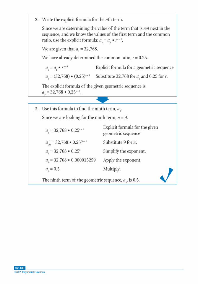
U2-130Unit 2: Polynomial Functions
2. Write the explicit formula for the nth term.
Since we are determining the value of the term that is not next in the sequence, and we know the values of the first term and the common ratio, use the explicit formula: a
n = a
1 • r n – 1.
We are given that a1 = 32,768.
We have already determined the common ratio, r = 0.25.
an = a
1 • r n – 1 Explicit formula for a geometric sequence
an = (32,768) • (0.25)n – 1 Substitute 32,768 for a
1 and 0.25 for r.
The explicit formula of the given geometric sequence is a
n = 32,768 • 0.25n – 1.
3. Use this formula to find the ninth term, a9.
Since we are looking for the ninth term, n = 9.
an = 32,768 • 0.25n – 1 Explicit formula for the given
geometric sequence
a(9)
= 32,768 • 0.25(9) – 1 Substitute 9 for n.
a9 = 32,768 • 0.258 Simplify the exponent.
a9 = 32,768 • 0.000015259 Apply the exponent.
a9 = 0.5 Multiply.
The ninth term of the geometric sequence, a9, is 0.5.

U2-131Lesson 5: Geometric Series
Example 5
You’re planning to experiment on a certain bacteria strain. It takes 1 hour for a cell of this strain to double. If you begin the experiment with 64 cells, how many cells will the experiment have exactly 1 day later?
1. Determine the common ratio.
The cells are doubling, which means that the common ratio, r, is 2.
2. Determine the value of a1.
The experiment begins with 64 bacteria cells, so a1 = 64.
3. Determine which geometric sequence formula to use: the recursive formula or the explicit formula.
We know the first term and the common ratio, so use the explicit formula.
4. Substitute values for the first term and the common ratio into the explicit formula to find the equation for the nth term.
The explicit formula for any geometric sequence is given by the equation a
n = a
1 • r n – 1.
We have already determined that r = 2 and a1 = 64. Use these values to
find the specific explicit formula for this sequence.
an = a
1 • r n – 1 Explicit equation for any geometric sequence
an = (64) • (2)n – 1 Substitute 2 for r and 64 for a
1.
The explicit equation for the nth term of the given geometric sequence is a
n = 64 • 2n – 1.
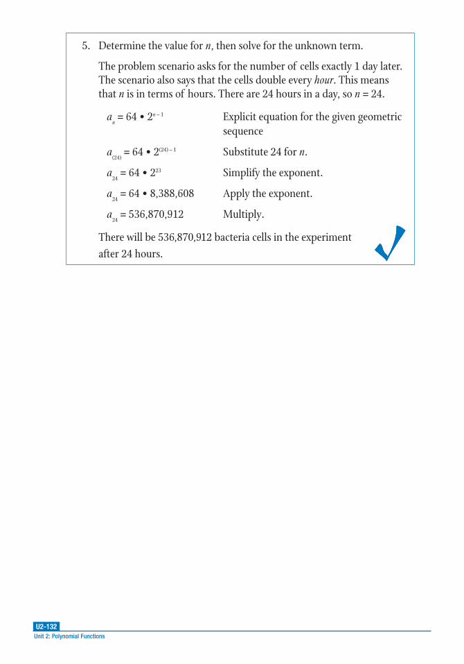
U2-132Unit 2: Polynomial Functions
5. Determine the value for n, then solve for the unknown term.
The problem scenario asks for the number of cells exactly 1 day later. The scenario also says that the cells double every hour. This means that n is in terms of hours. There are 24 hours in a day, so n = 24.
an = 64 • 2n – 1 Explicit equation for the given geometric
sequence
a(24)
= 64 • 2(24) – 1 Substitute 24 for n.
a24
= 64 • 223 Simplify the exponent.
a24
= 64 • 8,388,608 Apply the exponent.
a24
= 536,870,912 Multiply.
There will be 536,870,912 bacteria cells in the experiment after 24 hours.

UNIT 2 • POLYNOMIAL FUNCTIONSLesson 5: Geometric Series
PRACTICE
U2-133Lesson 5: Geometric Series
Find the missing terms in each sequence and state the common ratio, r.
1. {352, 176, 88, 44, a5, a
6, a
7, …}
2.
7
3,7, 21,63, , , ,5 6 7a a a
Find the specified term, an, using the given information.
3. a1 = 0.14, r = 2, n = 9
4. a1 = 64,
1
4r = , n = 6
5. 20
33a = , 5
3r = , n = 5
Write the explicit formula for the given sequence and find the specified term.
6.
10
9,
2
3,
2
5,
6
25, , ,6a
7. 6,9,27
2,
81
4, , ,7a
continued
Practice 2.5.1: Geometric Sequences

UNIT 2 • POLYNOMIAL FUNCTIONSLesson 5: Geometric Series
PRACTICE
U2-134Unit 2: Polynomial Functions
For problems 8–10, read each scenario and use the geometric sequence it describes to answer the questions.
8. A type of bacteria doubles in number every day. If you started with a culture of 50 cells, how many cells would you have after 8 days? What is the formula to determine how many cells you would have after n days?
9. A certain radioactive material has a half-life of 6 hours. If you have a sample of 120 mg of this material, how much of the material is left after 2 days of decay? What is the formula to determine how much material is left after n days?
10. Each swing of a particular pendulum is about 95% of the height of the previous swing. If the pendulum starts swinging from a height of 6 inches, after how many swings will the pendulum fall below a height of 3 inches?

U2-135Lesson 5: Geometric Series
IntroductionTerms of geometric sequences can be added together if needed, such as when calculating the total amount of money you will pay over the life of a loan that charges interest. When a group of some number of terms from a geometric sequence are added together, that group is called a geometric series. The number of terms in that group could go on forever, or the terms could be finite—that is, limited to a certain number. A finite geometric series is the sum of a specified number of terms of a geometric sequence. In this lesson, we will learn different ways to write and evaluate a finite geometric series.
Key Concepts
• A geometric series is the sum of some number of terms from a geometric sequence.
• Geometric sequences and series are related:
• Both have a common ratio.
• A sequence is a listing of the terms in a geometric progression.
• A series is the sum of part of that list.
• A finite series finds the sum of a specified number of the terms from the sequence.
• Compare the first five terms of the geometric sequence {1, 2, 4, 8, 16, …} with the same terms written as a geometric series:
Sequence: 1, 2, 4, 8, 16
Series: 1 + 2 + 4 + 8 + 16
• Summation notation is a symbolic way to represent the sum of a sequence.
• A common way to write summation notation for a geometric series is 11
1
a r k
k
n
∑ −
=
,
where n is a positive integer that represents the number of terms in the series, a1
is the first term, r is the common ratio, and k is the number of the term.
• This notation is read as “take the sum from 1 to n of the series a1 times r to the
k – 1.”
• The symbol ∑ is the uppercase Greek letter sigma. In this context, it means “to take the sum.”
Lesson 2.5.2: Sum of a Finite Geometric Series

U2-136Unit 2: Polynomial Functions
• The n represents the number of iterations to complete in the sum, or the final term in the sum. For example, if n = 3, you will add 3 of the terms in the series.
• k = 1 shows the starting value of the iterations, or the number of the term to start with in the sum.
• The diagram that follows illustrates the parts of this summation notation formula.
1
1
ar kk
n
∑ −
=
Number of terms
Starting term
Geometric sequenceTake the sum of
• Finite series have a definite ending term—they do not go on forever.
• Infinite series go to infinity. These will be explored later.
• Summing terms can be tedious. To make this process easier, mathematicians developed a formula for finding the sum of terms in a series; you will see the steps of how this formula is derived in Guided Practice Example 3.
• The sum formula for a finite geometric series from 1 to n is (1 )
11S
a r
rn
n
=−−
,
where Sn is the sum, a
1 is the first term, r is the common ratio, and n is the
number of terms.
• Notice that the right side of the formula is a fraction. The denominator of a fraction cannot equal 0. Therefore, in this formula, r ≠ 1.
Loan Payments and Sums of Finite Geometric Series
• The sum formula of a finite geometric series affects everyone who makes payments on a loan, whether they know it or not.
• When you take out a loan for a home or car, and pay interest on that loan, the total amount you will have paid by the time you make your last payment is actually the sum of a finite geometric series.
• Let’s say you take out a loan for a home. You will take out a loan for the price of the home, and make monthly payments to the lender. The bank that loaned you the money will charge interest each month until the loan is paid off. At the beginning of your loan, most of your payment goes to interest, because your
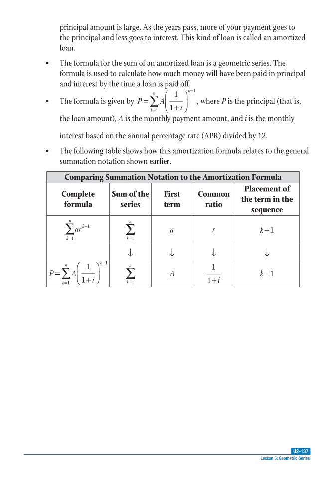
U2-137Lesson 5: Geometric Series
principal amount is large. As the years pass, more of your payment goes to the principal and less goes to interest. This kind of loan is called an amortized loan.
• The formula for the sum of an amortized loan is a geometric series. The formula is used to calculate how much money will have been paid in principal and interest by the time a loan is paid off.
• The formula is given by 1
11
1
P Aik
n k
∑= +
=
−
, where P is the principal (that is,
the loan amount), A is the monthly payment amount, and i is the monthly
interest based on the annual percentage rate (APR) divided by 12.
• The following table shows how this amortization formula relates to the general summation notation shown earlier.
Comparing Summation Notation to the Amortization Formula
Complete formula
Sum of the series
First term
Common ratio
Placement of the term in the
sequence
1
1
1
1
1
1
ar
P Ai
k
k
n
k
n k
∑
∑= +
−
=
=
−
1
1
k
n
k
n
Σ
Σ↓=
=
a
A
↓1
1
r
i
↓
+
1
1
k
k
−
↓−
1
1
k
n
k
n
Σ
Σ↓=
=
a
A
↓1
1
r
i
↓
+
1
1
k
k
−
↓−1
1
1
1
1
1
ar
P Ai
k
k
n
k
n k
∑
∑= +
−
=
=
−
1
1
k
n
k
n
Σ
Σ↓=
=
a
A
↓1
1
r
i
↓
+
1
1
k
k
−
↓−
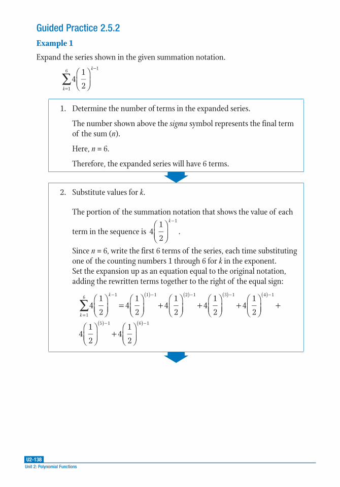
U2-138Unit 2: Polynomial Functions
Example 1
Expand the series shown in the given summation notation.
41
21
6 1
k
k
∑
=
−
1. Determine the number of terms in the expanded series.
The number shown above the sigma symbol represents the final term of the sum (n).
Here, n = 6.
Therefore, the expanded series will have 6 terms.
2. Substitute values for k.
The portion of the summation notation that shows the value of each
term in the sequence is 41
2
1k
−
.
Since n = 6, write the first 6 terms of the series, each time substituting one of the counting numbers 1 through 6 for k in the exponent. Set the expansion up as an equation equal to the original notation, adding the rewritten terms together to the right of the equal sign:
41
24
1
24
1
24
1
24
1
24
1
24
1
21
6 1 1 1 2 1 3 1 4 1 5 1 6 1
k
k
∑
=
+
+
+
+
+
( ) ( ) ( ) ( ) ( ) ( )
=
− − − − − − −
41
24
1
24
1
24
1
24
1
24
1
24
1
21
6 1 1 1 2 1 3 1 4 1 5 1 6 1
k
k
∑
=
+
+
+
+
+
( ) ( ) ( ) ( ) ( ) ( )
=
− − − − − − −
Guided Practice 2.5.2
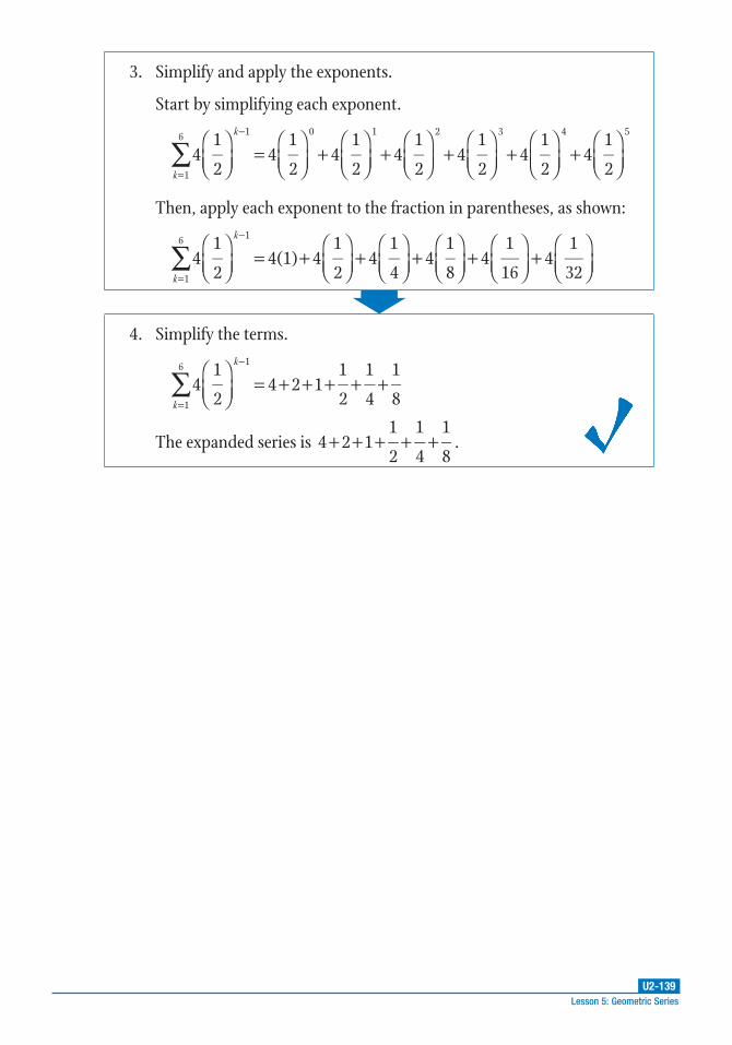
U2-139Lesson 5: Geometric Series
3. Simplify and apply the exponents.
Start by simplifying each exponent.
41
24
1
24
1
24
1
24
1
24
1
24
1
21
6 1 0 1 2 3 4 5
k
k
∑
=
+
+
+
+
+
=
−
Then, apply each exponent to the fraction in parentheses, as shown:
41
24(1) 4
1
24
1
44
1
84
1
164
1
321
6 1
k
k
∑
= +
+
+
+
+
=
−
4. Simplify the terms.
41
24 2 1
1
2
1
4
1
81
6 1
k
k
∑
= + + + + +=
−
The expanded series is 4 2 11
2
1
4
1
8+ + + + + .

U2-140Unit 2: Polynomial Functions
Example 2
Sum the series by expansion.
2(3) 1
1
5k
k∑ −
=
1. Expand the series.
k = 1 and n = 5; therefore, the series starts with the first term of the sequence and ends with the fifth term.
Write the first 5 terms of the series, each time substituting one of the counting numbers 1 through 5 for k in the exponent as shown:
∑ = + + + +−
=
− − − − −k
k
2(3) 2(3) 2(3) 2(3) 2(3) 2(3)1
1
5(1) 1 ( 2) 1 (3) 1 ( 4) 1 (5) 1
Simplify and apply the exponents to each term.
2(3) 2(3) 2(3) 2(3) 2(3) 2(3)1
1
50 1 2 3 4k
k∑ = + + + +−
=
Simplify the exponents.
2(3) 2(1) 2(3) 2(9) 2(27) 2(81)1
1
5k
k∑ = + + + +−
=
Apply the exponents.
Notice that each term has a factor of 2.
2. Factor the expression and simplify.
2(3) 2(1) 2(3) 2(9) 2(27) 2(81)1
1
5k
k∑ = + + + +−
=
Series with exponents applied
2(3) 2 1 3 9 27 811
1
5k
k∑ ( )= + + + +−
=
Factor out 2 from the terms in the series.
2(3) 2 1211
1
5k
k∑ ( )=−
=Sum the terms.
2(3) 2421
1
5k
k∑ =−
=Multiply.
The sum of the series containing the first 5 terms of the sequence is 242.
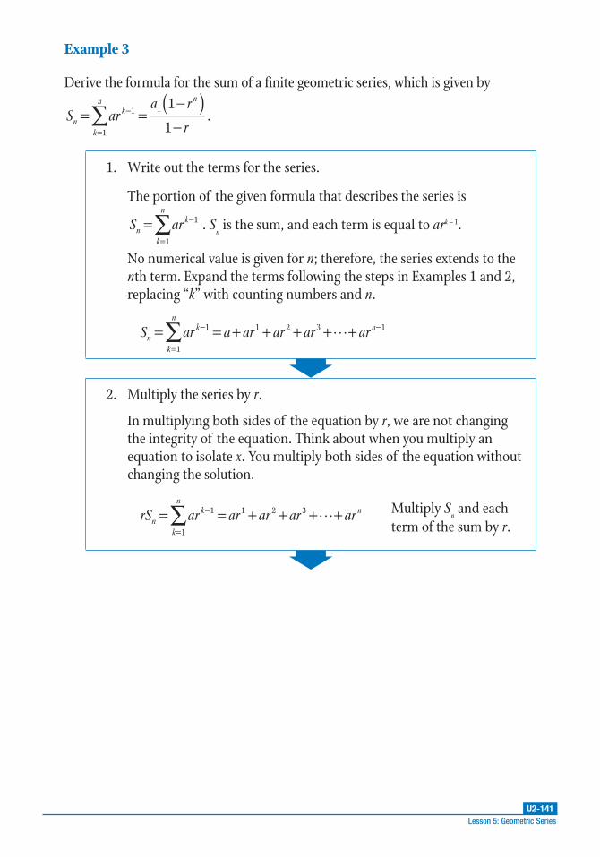
U2-141Lesson 5: Geometric Series
Example 3
Derive the formula for the sum of a finite geometric series, which is given by 1
11 1
1
S ara r
rnk
n
k
n
∑ ( )= =
−−
−
=
.
1. Write out the terms for the series.
The portion of the given formula that describes the series is 1
1
S arnk
k
n
∑= −
=
. Sn is the sum, and each term is equal to ark – 1.
No numerical value is given for n; therefore, the series extends to the nth term. Expand the terms following the steps in Examples 1 and 2, replacing “k” with counting numbers and n.
∑= = + + + + +−
=
−S ar a ar ar ar arnk
k
nn1
1
1 2 3 1
2. Multiply the series by r.
In multiplying both sides of the equation by r, we are not changing the integrity of the equation. Think about when you multiply an equation to isolate x. You multiply both sides of the equation without changing the solution.
∑= = + + + +−
=
rS ar ar ar ar arnk
k
nn1
1
1 2 3
Multiply Sn and each
term of the sum by r.
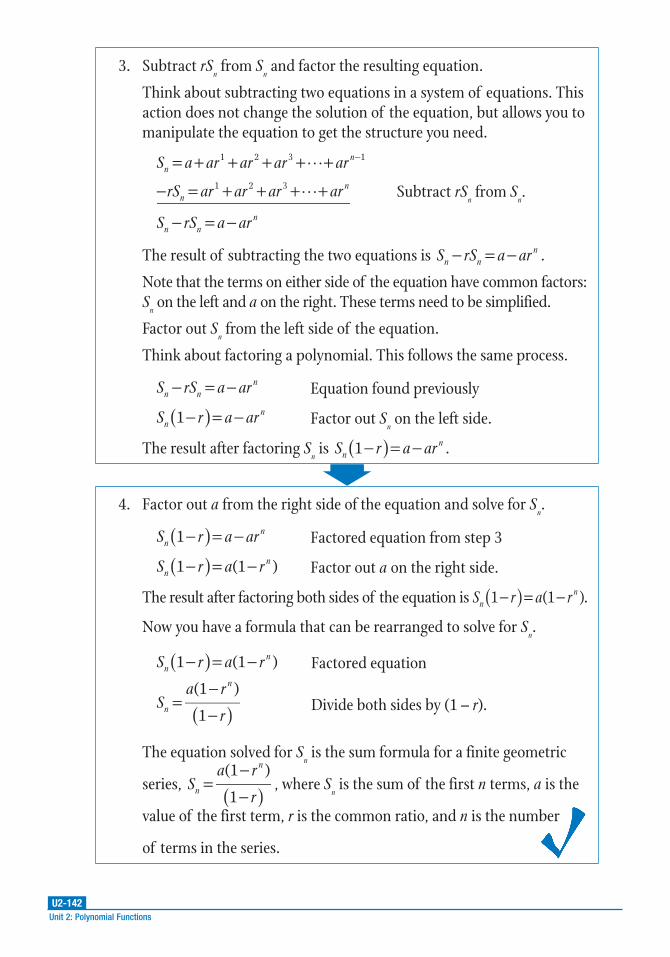
U2-142Unit 2: Polynomial Functions
3. Subtract rSn from S
n and factor the resulting equation.
Think about subtracting two equations in a system of equations. This action does not change the solution of the equation, but allows you to manipulate the equation to get the structure you need.
= + + + + +
− = + + + +
− = −
−S a ar ar ar ar
rS ar ar ar ar
S rS a ar
nn
nn
n nn
1 2 3 1
1 2 3
Subtract rSn from S
n.
The result of subtracting the two equations is S rS a arn nn− = − .
Note that the terms on either side of the equation have common factors: S
n on the left and a on the right. These terms need to be simplified.
Factor out Sn from the left side of the equation.
Think about factoring a polynomial. This follows the same process.
S rS a arn nn− = − Equation found previously
1S r a arnn( )− = − Factor out S
n on the left side.
The result after factoring Sn is 1S r a arn
n( )− = − .
4. Factor out a from the right side of the equation and solve for Sn.
1S r a arnn( )− = − Factored equation from step 3
1 (1 )S r a rnn( )− = − Factor out a on the right side.
The result after factoring both sides of the equation is 1 (1 )S r a rnn( )− = − .
Now you have a formula that can be rearranged to solve for Sn.
1 (1 )S r a rnn( )− = − Factored equation
(1 )
1S
a r
rn
n
( )=−− Divide both sides by (1 – r).
The equation solved for Sn is the sum formula for a finite geometric
series, (1 )
1S
a r
rn
n
( )=−−
, where Sn is the sum of the first n terms, a is the
value of the first term, r is the common ratio, and n is the number
of terms in the series.

U2-143Lesson 5: Geometric Series
Example 4
Sum the given series using the sum formula for a finite geometric series.
3(2)1
61
k
k∑=
−
1. Write the sum formula and identify the variables that need to be substituted.
(1 )
11S
a r
rn
n
( )=−−
The following variables need to be substituted:
• a1 (the first term in the series)
• r (the common ratio)
• n (the number of terms in the series)
Examine the summation notation to determine values for a1, r, and n.
2. Calculate the value of the first term, a1.
In the given series 3(2)1
61
k
k∑=
− , substitute the counting number 1 for k
and evaluate to find the value of the first term.
a1 = 3(2)k – 1 = 3(2)(1) – 1 = 3(2)0 = 3(1) = 3
The value of the first term, a1, is 3.
3. Determine the common ratio, r.
Remember the formula for a geometric sequence, an = a • r n – 1, where
r is the common ratio. Each term in this series is equal to 3(2)k – 1. Therefore, the common ratio is 2.
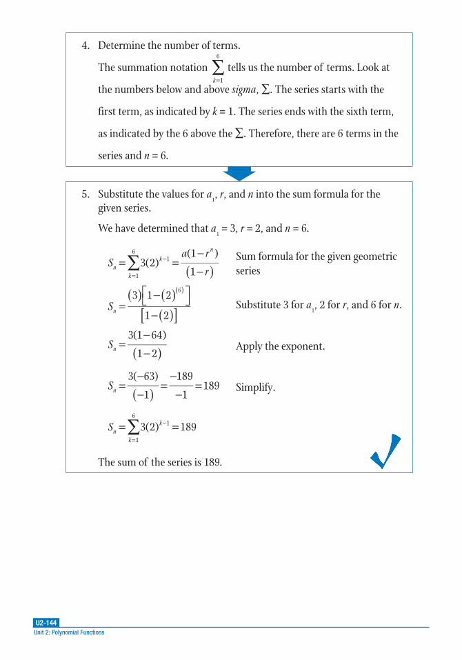
U2-144Unit 2: Polynomial Functions
4. Determine the number of terms.
The summation notation 1
6
k∑=
tells us the number of terms. Look at
the numbers below and above sigma, ∑. The series starts with the
first term, as indicated by k = 1. The series ends with the sixth term,
as indicated by the 6 above the ∑. Therefore, there are 6 terms in the
series and n = 6.
5. Substitute the values for a1, r, and n into the sum formula for the
given series.
We have determined that a1 = 3, r = 2, and n = 6.
3(2)(1 )
11
1
6
Sa r
rnk
k
n
∑ ( )= =−−
−
=
Sum formula for the given geometric series
3 1 2
1 2
6
Sn [ ]( ) ( )
( )=− −
( )
Substitute 3 for a1, 2 for r, and 6 for n.
3(1 64)
1 2Sn ( )=
−−
Apply the exponent.
3( 63)
1
189
1189Sn ( )=
−−
=−−
= Simplify.
3(2) 1891
61Sn
k
k∑= ==
−
The sum of the series is 189.

U2-145Lesson 5: Geometric Series
Example 5
Seline is applying for a $10,000 college loan to be repaid over 10 years. The annual
percentage rate (APR) on the loan is 3%. However, the interest on the loan is
compounded monthly. The amount Seline will owe can be found using the formula for
the sum of an amortized loan, 1
11
1
P Aik
n k
∑= +
=
−
, where:
P = loan amount (principal)
A = monthly payment amount
i = monthly interest rate of the loan
n = number of monthly payments
Use the formula to determine Seline’s monthly payment amount, A.
1. Use the given information to determine values for P, i, and n.
The problem statement tells us that the loan is for $10,000, so P = 10,000.
The yearly interest rate is 3%, compounded monthly. Divide 3% (0.03) by 12 to find the monthly interest rate, i.
0.03
120.0025i = =
Seline will make 12 payments each year for 10 years. Multiply 12 by 10 to determine the total number of monthly payments, n.
10 years12 months
1 year120 monthsn= • =

U2-146Unit 2: Polynomial Functions
2. Apply the sum formula for a finite geometric series.
The formula for the sum of a finite geometric series is (1 )
11S
a r
rn
n
=−−
.
Set the amortization formula, 1
11
1
P Aik
n k
∑= +
=
−
, equal to the sum formula.
1
1
(1 )
11
11P A
i
a r
rk
n k n
∑ ( )=+
=−−=
−
This formula simplifies to (1 )
11P
a r
r
n
( )=−−
.
In this formula, we know the following variables:
P = 10,000
n = 120
We also know that 1
1 i+ in the amortization formula corresponds to r
in summation notation, so 1
1r
i=
+.
We don’t know the value of the first term, a1.
Recall that the variable a in summation notation, 1
1
ar k
k
n
∑ −
=
,
corresponds to A in the amortization formula, 1
11
1
P Aik
n k
∑= +
=
−
.
To find A, we must first solve the formula for the sum of this loan, (1 )
11P
a r
r
n
( )=−−
, for a1.

U2-147Lesson 5: Geometric Series
3. Rearrange the sum formula to solve for a1.
(1 )
11P
a r
r
n
( )=−−
Formula for the sum of the loan
1
(1 )
(1 )
1
1
(1 )1Pr
ra
r
r
r
rn
n
n
( )( )
( )•
−−
=−−
•−−
Multiply both sides by the reciprocal of the fraction.
1
(1 ) 1Pr
ran
( )−−
= Simplify.
1
(1 )1a Pr
r n
( )=
−−
Use the symmetric property of equality to switch sides.
The formula is now solved for the value of the first term, a1.
4. Calculate r.
From step 2, we know that 1
1r
i=
+. From step 1, we know that
i = 0.0025.
Substitute this value for i and solve.
1
1
1
1 0.0025
1
1.00250.998r
i=
+=
+= ≈
Now we have the values we need to determine Seline’s monthly payment:
a1 = A = monthly payment amount
P = 10,000
r = 0.998
n = 120

U2-148Unit 2: Polynomial Functions
5. Substitute the values into the formula 1
(1 )1a Pr
r n
( )=
−−
.
1
(1 )1a Pr
r n
( )=
−−
Formula
10,0001 0.998
(1 0.998 )120A( )
=−−
Substitute A for a
1, 10,000 for P,
0.998 for r, and 120 for n.
10,0000.002
(1 0.786)A
( )=
− Simplify.
10,0000.002
0.214=
A Continue to simplify.
A ≈ 10,000(0.00935)
A ≈ 93.458
Seline’s monthly payment will be about $93.46.

UNIT 2 • POLYNOMIAL FUNCTIONSLesson 5: Geometric Series
PRACTICE
U2-149Lesson 5: Geometric Series
Expand the series.
1. 481
2
1
1
7 k
k∑
−
=
Evaluate the series using expansion.
2. 94
3
1
1
5 k
k∑
−
=
Evaluate the series using the sum formula.
3. 21
6
1
1
5 k
k∑
−
=
Find the first term of the series given the sum, the common ratio, and the number of terms.
4. Sn = 30,000, r = 0.993, n = 36
Read each scenario and use the given information to answer the questions.
5. A laboratory keeps a supply of a certain radioactive material that has a half-life of 1 month. If after 1 month only 160 mg of the material remain in stock, how much will have decayed after the eighth month?
6. Hassan has become a renowned accordionist. He realizes that in his 10-year career, his income has steadily increased by 15% each year. If his income the first year was $12,000, how much has he earned over the past 10 years playing the accordion? Round to the nearest cent.
continued
Practice 2.5.2: Sum of a Finite Geometric Series
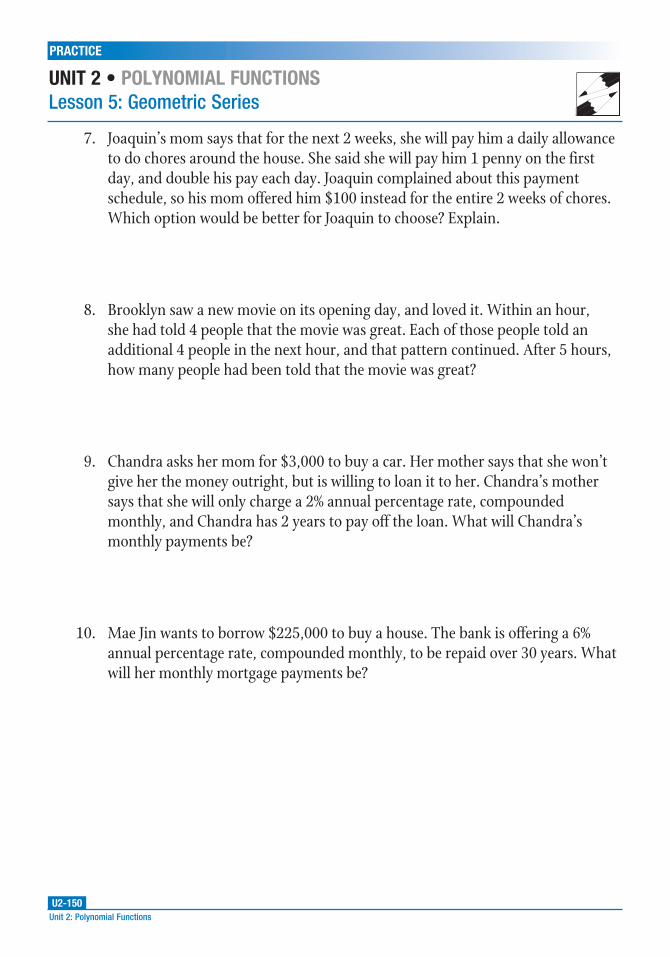
UNIT 2 • POLYNOMIAL FUNCTIONSLesson 5: Geometric Series
PRACTICE
U2-150Unit 2: Polynomial Functions
7. Joaquin’s mom says that for the next 2 weeks, she will pay him a daily allowance to do chores around the house. She said she will pay him 1 penny on the first day, and double his pay each day. Joaquin complained about this payment schedule, so his mom offered him $100 instead for the entire 2 weeks of chores. Which option would be better for Joaquin to choose? Explain.
8. Brooklyn saw a new movie on its opening day, and loved it. Within an hour, she had told 4 people that the movie was great. Each of those people told an additional 4 people in the next hour, and that pattern continued. After 5 hours, how many people had been told that the movie was great?
9. Chandra asks her mom for $3,000 to buy a car. Her mother says that she won’t give her the money outright, but is willing to loan it to her. Chandra’s mother says that she will only charge a 2% annual percentage rate, compounded monthly, and Chandra has 2 years to pay off the loan. What will Chandra’s monthly payments be?
10. Mae Jin wants to borrow $225,000 to buy a house. The bank is offering a 6% annual percentage rate, compounded monthly, to be repaid over 30 years. What will her monthly mortgage payments be?

U2-151Lesson 5: Geometric Series
IntroductionWe have seen series that are finite, meaning they have a limited number of terms, but what happens to a series that has infinite terms? A geometric series that has infinite terms (that is, where n=∞ ), is called an infinite geometric series. In an infinite geometric series, summing all the terms in the series is not an easy task, because the series starts with n = 1 and goes on until infinity. Do such sums exist? As you will see in this lesson, for infinite geometric series with certain values of the common ratio r, a sum does exist.
Key Concepts
• Whether an infinite geometric series has a sum depends on whether the absolute value of its common ratio, r, is greater or less than 1, and on the behavior of the partial sums of the series.
• Partial sums are the sums of part of a series. They are the result of adding pairs of terms. Partial sums are used to determine if a series converges or diverges.
• In a series, to converge means to approach a finite limit. If the sequence of the partial sums of a series approaches the value of a given number (the limit), then the entire series converges to that limit. In other words, the series has a sum.
• An infinite series converges when the absolute value of the common ratio r is less than 1 1r( )< .
• If the series does not have a sum—that is, the sequence of its partial sums does not approach a finite limit—then the series is said to diverge.
• In a series that diverges, the absolute value of the common ratio, r, is greater than 1 1r( )> .
• Recall that a series cannot have an r value equal to 1 (r ≠ 1), because this would result in a 0 in the denominator of the sum formula. Fractions with a denominator of 0 are undefined.
• Consider the sequence 1
3
1
3
1
an
n
= •
−
. The terms and the partial sums of the
series from n = 1 to n = 8 are calculated in the table that follows.
Lesson 2.5.3: Sum of an Infinite Geometric Series
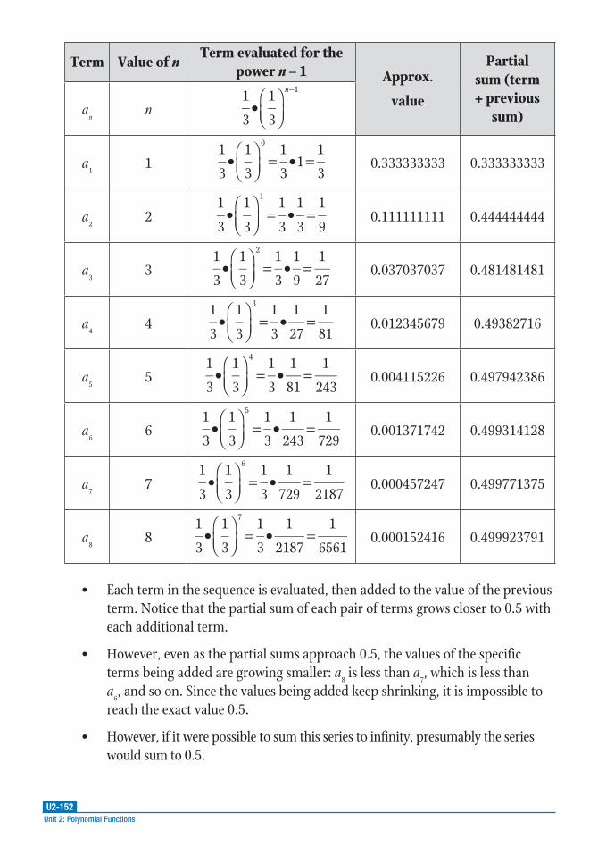
U2-152Unit 2: Polynomial Functions
Term Value of nTerm evaluated for the
power n – 1 Approx.
value
Partial sum (term + previous
sum)an
n1
3
1
3
1
•
−n
a1
11
3
1
3
1
31
1
3
0
•
= • = 0.333333333 0.333333333
a2
21
3
1
3
1
3
1
3
1
9
1
•
= • = 0.111111111 0.444444444
a3
31
3
1
3
1
3
1
9
1
27
2
•
= • = 0.037037037 0.481481481
a4
41
3
1
3
1
3
1
27
1
81
3
•
= • = 0.012345679 0.49382716
a5
51
3
1
3
1
3
1
81
1
243
4
•
= • = 0.004115226 0.497942386
a6
61
3
1
3
1
3
1
243
1
729
5
•
= • = 0.001371742 0.499314128
a7
71
3
1
3
1
3
1
729
1
2187
6
•
= • = 0.000457247 0.499771375
a8
81
3
1
3
1
3
1
2187
1
6561
7
•
= • = 0.000152416 0.499923791
• Each term in the sequence is evaluated, then added to the value of the previous term. Notice that the partial sum of each pair of terms grows closer to 0.5 with each additional term.
• However, even as the partial sums approach 0.5, the values of the specific terms being added are growing smaller: a
8 is less than a
7, which is less than
a6, and so on. Since the values being added keep shrinking, it is impossible to
reach the exact value 0.5.
• However, if it were possible to sum this series to infinity, presumably the series would sum to 0.5.
U2-153Lesson 5: Geometric Series
• The sum formula for an infinite geometric series, if the sum exists, is given
by 1
1Sa
rn = −, where S
n is the sum, a
1 is the first term, and r is the common
ratio. Guided Practice Example 1 shows how this formula is derived from the
sum formula for a finite geometric series.
• If the series converges—that is, if 1r < —then the sum exists and this formula can be used to find it.
• Recall that the summation notation for a finite geometric series is 1
1
ar k
k
n
∑ −
=
,
where n is the number of terms in the sequence.
• An infinite series in summation notation has an infinity symbol ( )∞ above the sigma instead of n to indicate an unlimited number of terms:
1
1
ar k
k∑ −
=
∞

U2-154Unit 2: Polynomial Functions
Example 1
Derive the formula for the sum of infinite series, 1
1Sa
rn = −, if 1r < . Base the
derivation on the sum formula for a finite series.
1. Write the formula for the sum of a finite series.
(1 )
11S
a r
rn
n
=−−
Here, Sn is the sum, a
1 is the first term of the series, r is the common
ratio, and n is the number of terms.
2. Distribute the first term in the numerator.
11 1S
a a r
rn
n
=−−
3. Rewrite the fraction as the difference of two fractions.
1 11 1S
a
r
a r
rn
n
=−
−−
4. Substitute an infinity symbol for the exponent, n.
The infinity symbol, ∞ , indicates an unlimited number of terms.
1 11 1S
a
r
a r
rn = −−
−
∞
Guided Practice 2.5.3

U2-155Lesson 5: Geometric Series
5. Analyze the effect of raising a value of 1r < to an infinite power.
Recall the table of partial sums of the sequence 1
3
1
3
1
an
n
= •
−
shown
in the Key Concepts. In that sequence, 1
3r = , the absolute value of
which is less than 1. The table showed that the value of each new term
in the series was smaller than the last, approaching 0. This is true for
any value of r when the absolute value of r is less than 1.
Therefore, as the power applied to r approaches infinity, r approaches 0.
6. Simplify the formula using the process of raising r, where 1r < , to a power of ∞ .
1 11 1S
a
r
a r
rn = −−
−
∞
Sum formula from step 4
1
(0)
11 1S
a
r
a
rn = −−
− Substitute 0 for r∞ .
1
0
11S
a
r rn = −−
− Simplify by subtracting the numerators.
11S
a
rn = −
The formula for the sum of infinite geometric series, where
1r < , is 1
1Sa
rn = −.
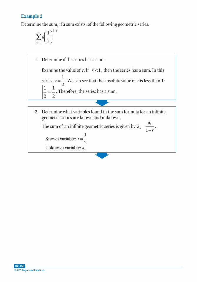
U2-156Unit 2: Polynomial Functions
Example 2
Determine the sum, if a sum exists, of the following geometric series.
41
21
1
k
k
∑
=
∞ −
1. Determine if the series has a sum.
Examine the value of r. If 1r < , then the series has a sum. In this
series, 1
2r = . We can see that the absolute value of r is less than 1:
1
2
1
2= . Therefore, the series has a sum.
2. Determine what variables found in the sum formula for an infinite geometric series are known and unknown.
The sum of an infinite geometric series is given by 1
1Sa
rn = −.
Known variable: 1
2r =
Unknown variable: a1

U2-157Lesson 5: Geometric Series
3. Determine the value of a1 in the series.
41
21
1
k
k
∑
=
∞ −
Given series
41
24
1
21
1 1 0
k∑
=
+
=
∞ −Write out the first term and substitute 1 for k.
41
24(1) 4
0
= = Simplify.
The first term of the series is 4.
The geometric series is given by a • r n – 1. The first term has an n value of 1, which makes the power 0. Anything raised to a power of 0 is 1. This means that you will be multiplying the value of a by 1, which just results in a.
4. Substitute the variables into the sum formula for an infinite geometric series.
Known values: r1
2= , a
1 = 4
11S
a
rn = −Sum formula for an infinite geometric series
4
11
2
=−
Sn Substitute 1
2 for r.
41
2
4•2 8Sn = = = Simplify.
The infinite series 41
21
1
k
k
∑
=
∞ −
sums to 8.
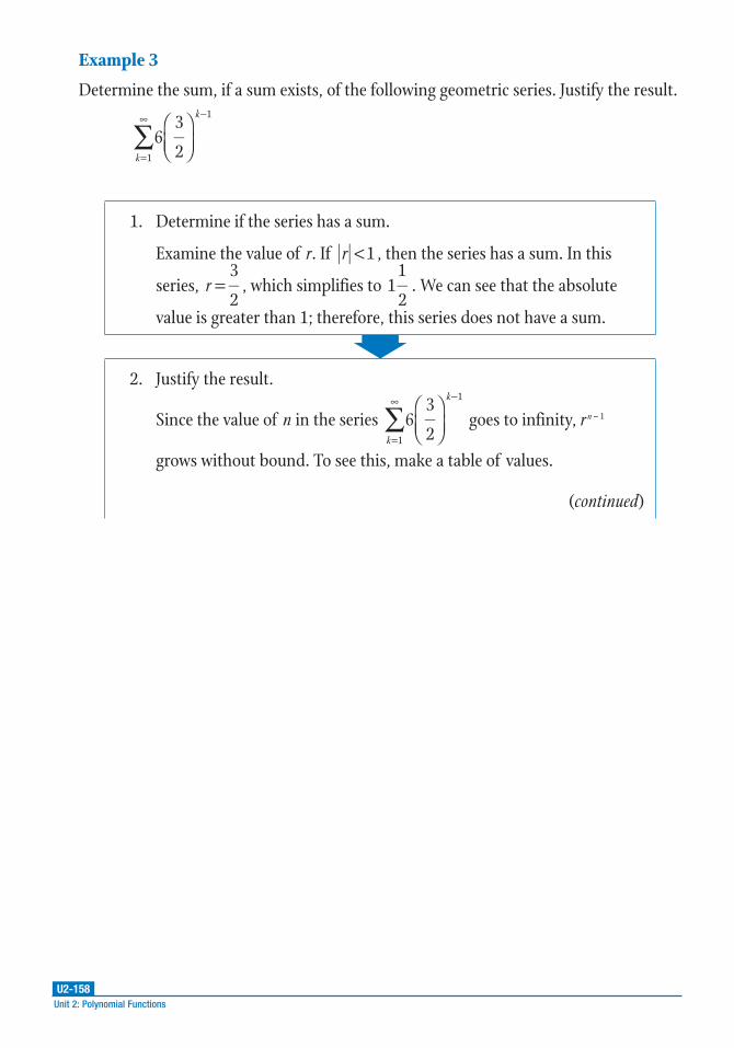
U2-158Unit 2: Polynomial Functions
Example 3
Determine the sum, if a sum exists, of the following geometric series. Justify the result.
63
21
1
k
k
∑
=
∞ −
1. Determine if the series has a sum.
Examine the value of r. If 1r < , then the series has a sum. In this
series, 3
2r = , which simplifies to 1
1
2. We can see that the absolute
value is greater than 1; therefore, this series does not have a sum.
2. Justify the result.
Since the value of n in the series 63
21
1
k
k
∑
=
∞ −
goes to infinity, r n – 1
grows without bound. To see this, make a table of values.
(continued)

U2-159Lesson 5: Geometric Series
TermValue of n
Term evaluated for the power n – 1 Approx.
value
Partial sum (term + previous
sum)an
n 63
2
1n
−
a1
1 63
26(1)
0
= 6 6
a2
2 63
26
3
2
18
29
1
=
= = 9 15
a3
3 63
26
9
4
54
413.5
2
=
= = 13.5 28.5
a4
4 63
26
27
8
162
820.25
3
=
= = 20.25 48.75
a5
5 63
26
81
16
486
1630.375
4
=
= = 30.375 79.125
a6
6 63
26
243
32
1458
3245.5625
5
=
= = 45.5625 124.6875
a7
7 63
26
729
64
4374
6468.34375
6
=
= = 68.34375 193.03125
a8
8 63
26
2187
128
13,122
128102.515625
8
=
= = 102.515625 295.546875
We can see that the partial sums do not converge to a limit; they increase in value infinitely. Since the partial sums do not converge, this series is diverging and has no sum. The result found in step 1 is justified.

U2-160Unit 2: Polynomial Functions
Example 4
Use the formula for an infinite geometric series to rewrite 0.6 as a fraction.
1. Write the repeating decimal as a sum.
0.6 = 0.6 + 0.06 + 0.006 + …
Notice that this is a geometric sequence because there is a common ratio r between each term and the next.
2. Determine the value of r.
Substitute the values for a2 and a
1 into the formula for the common
ratio r.
0.06
0.60.1
1
101
ra
an
n
( )( )= = = =
−
The value of r is 1
10.
3. Write the sum of the series using summation notation.
Known values: a1 = 0.6,
1
10r =
1
1
ar k
k∑ −
=
∞ General summation notation for an infinite geometric series
0.61
10
1
1
k
k∑( )
−
=
∞
Substitute 0.6 for a1
and 1
10 for r.
The repeating decimal 0.6 written using summation notation is
0.61
10
1
1
k
k∑
−
=
∞.

U2-161Lesson 5: Geometric Series
4. Evaluate the series using the sum formula.
11S
a
rn = −Sum formula for an infinite geometric series
0.6
11
10
=−
Sn
Substitute 0.6 for a1
and 1
10 for r.
0.69
10
6
109
10
Sn = = Write 0.6 as a fraction in the numerator.
6
109
10
6
10
10
9
6
9
2
3Sn = = • = = Simplify.
0.6 written as a fraction is 2
3.

UNIT 2 • POLYNOMIAL FUNCTIONSLesson 5: Geometric Series
PRACTICE
U2-162Unit 2: Polynomial Functions
Determine the sum of each series, if a sum exists. If no sum exists, write “No sum exists.”
1. 1
4
1
31
1
k
k
∑
=
∞ −
2. 51
41
1
k
k
∑
=
∞ −
3. 75
41
1
k
k
∑
=
∞ −
4. 0.39 0.21
1
k
k∑ ( )=
∞−
5. 9 + 6 + 4 + …
6.
7
4
21
8
63
16+ + +
Read the scenario below and use it to solve problems 7 and 8.
Randall is setting up a large tent for his son’s graduation party. The directions for the tent recommend that the stakes be driven into the ground at least 6 inches. The first time Randall strikes a stake with his mallet, he drives the stake into the ground 4 inches. On each of his subsequent strikes, he is only able to drive the stake into the ground 32% of the distance of the previous strike.
7. Write an infinite geometric series that represents how far Randall can drive the stake into the ground.
8. Can Randall drive the stake into the ground the recommended 6 inches? Explain.
Practice 2.5.3: Sum of an Infinite Geometric Series
continued

UNIT 2 • POLYNOMIAL FUNCTIONSLesson 5: Geometric Series
PRACTICE
U2-163Lesson 5: Geometric Series
Read the scenario below and use it to solve problems 9 and 10.
The midsegment of a triangle connects the two midpoints of two sides of a triangle and is equal to half the distance of the third side. Abbie uses illustration software to draw an equilateral triangle with side lengths of 9 cm each, then draws a smaller triangle inside it by connecting the midpoints of the triangle. Using the software, she can repeat this pattern indefinitely.
9 cm9 cm
9 cm
9. Write an infinite geometric series that describes the area of all the triangles that
Abbie can draw by repeatedly joining the midsegments of a triangle. (Hint: Use
the formula for the area of an equilateral triangle: 3
4
2
As
= .)
10. Evaluate the series from problem 9.

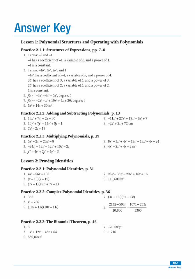
AK-1Answer Key
Answer KeyLesson 1: Polynomial Structures and Operating with Polynomials
Practice 2.1.1: Structures of Expressions, pp. 7–81. Terms: –k and –1.
–k has a coefficient of –1, a variable of k, and a power of 1. –1 is a constant.2.
3. Terms: –4b4, 3b3, 2b2, and 1. –4b4 has a coefficient of –4, a variable of b, and a power of 4. 3b3 has a coefficient of 3, a variable of b, and a power of 3. 2b2 has a coefficient of 2, a variable of b, and a power of 2. 1 is a constant.4.
5. f(x) = –3x5 – 6x3 – 5x2; degree: 56.
7. f(x) = –2x6 – x5 + 10x3 + 4x + 20; degree: 68.
9. 5x2 + 14x + 30 in2
Practice 2.1.2: Adding and Subtracting Polynomials, p. 131. 13x6 + 7x2 + 2x + 302.
3. 16y4 + 7y3 + 14y2 + 8y – 14.
5. 7z2 – 2z + 136.
7. –11x6 + 27x4 + 19x3 – 6x2 + 78.
9. –2x2 + 2x + 72 cm
Practice 2.1.3: Multiplying Polynomials, p. 191. 5x5 – 2x3 + 20x2 – 82.
3. –24z5 + 12z4 – 12z3 + 10z2 – 2z4.
5. y10 – 4y7 + 2y5 + 4y2 – 36.
7. 8x7 – 3x6 + 4x4 – 45x3 – 18x2 – 4x – 248.
9. 4x3 – 2x2 + 4x – 2 m2
Lesson 2: Proving Identities
Practice 2.2.1: Polynomial Identities, p. 311. 4x2 – 56x + 1962.
3. (x – 19)(x + 19)4.
5. (7x – 1)(49x2 + 7x + 1)6.
7. 25x4 – 36x2 – 20x3 + 16x + 168.
9. 115,600 in2
Practice 2.2.2: Complex Polynomial Identities, p. 361. 3622.
3. x2 + 2564.
5. (10x + 11i)(10x – 11i)6.
7. (3x + 13i)(3x – 13i)8.
9. i i2142 506
10,600
1071 253
5300
−=
−
Practice 2.2.3: The Binomial Theorem, p. 461. 32.
3. –x3 + 12x2 – 48x + 644.
5. 589,824x76.
7. –2912x3y118.
9. 1,716
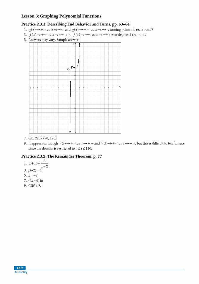
AK-2Answer Key
Lesson 3: Graphing Polynomial Functions
Practice 2.3.1: Describing End Behavior and Turns, pp. 63–641. ( )g x →+∞ as x→−∞ and g x( )→−∞ as x→+∞ ; turning points: 6; real roots: 72.
3. ( )f x →+∞ as x→−∞ and ( )f x →+∞ as x→+∞ ; even-degree; 2 real roots4.
5. Answers may vary. Sample answer:
f(x)
6.
7. (50, 220), (70, 125)8.
9. It appears as though →+∞V t( ) as t→+∞ and →+∞V t( ) as t→−∞ , but this is difficult to tell for sure since the domain is restricted to 0 ≤ t ≤ 110.
Practice 2.3.2: The Remainder Theorem, p. 77
1. 1030
2x
x+ +
−2.
3. p(–2) = 44.
5. k = –66.
7. (4x – 6) in8.
9. 0.5t2 + 8t

AK-3Answer Key
Practice 2.3.3: Finding Zeros, p. 871. 3 real roots; –4, –2, 2 2.
3. 1 real root, 2 imaginary roots; 2, 1 – 2i, 1 + 2i4.
5. x = –3, x = –1, x = 4
–10 –9 –8 –7 –6 –5 –4 –3 –2 –1 0 1 2 3 4 5 6 7 8 9 10
–30
–28
–26
–24
–22
–20
–18
–16
–14
–12
–10
–8
–6
–4
–2
2
4
6
8
10
f(x)
6.
7. f(x) = (x + 3)(x + 2)(x – 1)(x – 5) = x4 – x3 – 19x2 – 11x + 308.
9. f(x) = (x + 8)(x – 4)x = 4608 or f(x) = x3 + 4x2 – 32x = 4608
Practice 2.3.4: The Rational Root Theorem, p. 941. ±1, ±7
2.
3. 1
6,
1
3,
1
2, 1± ± ± ±
4.
5. 2, 1,5
2− −
6.
7. 3, 1 3, 1 3− +8.
9. x3 – 5x2 – 3x + 15

AK-4Answer Key
Lesson 4: Solving Systems of Equations with Polynomials
Practice 2.4.1: Solving a Linear-Polynomial System of Equations, pp. 114–1151. {(–1, 3), (3, 7), (8, 12)}
–5 –4 –3 –2 –1 0 1 2 3 4 5 6 7 8 9 10
–45
–40
–35
–30
–25
–20
–15
–10
–5
5
10
15
20
25
30
35
40
45
f(x)
g(x)
2.
3. {(–3, –76)}
–5 –4 –3 –2 –1 0 1 2 3 4 5
–300
–250
–200
–150
–100
–50
50
100
150
200
250
300
f(x)
g(x)
4.
5. It appears as though there are no real solutions to this system of equations because the differences in values for f(x) and g(x) do not approach 0. In other words, the graphs of these two values, f(x) and g(x), never get close enough to each other to intersect.6.
7. {(0, –5)}8.
9. The deer population was at a healthy level of 10 bucks per square mile for the surveys that covered 1, 2, 4, and 5 square miles of the wildlife preserve.

AK-5Answer Key
Lesson 5: Geometric Series
Practice 2.5.1: Geometric Sequences, pp. 133–1341. 22, 11, 5.5; r = 0.52.
3. a9 = 35.844.
5. a5 = 500/276.
7. an = 6 • (3/2)n – 1; a
6 = 68.343758.
9. 0.9375 mg; an = 120 • (1/2)n – 1
Practice 2.5.2: Sum of a Finite Geometric Series, pp. 149–1501. 48 + 24 + 12 + 6 + 4 + 1.5 + 0.752.
3. 2.399691364.
5. 318.75 mg6.
7. It would be better for Joaquin to take the first payment option his mother offered, because that option would pay out $163.83, which is more than a flat fee of $100.8.
9. about $127.90
Practice 2.5.3: Sum of an Infinite Geometric Series, pp. 162–1631. 3/82.
3. No sum exists.4.
5. 276.
7. 432
1001
1
k
k
∑
=
∞ −
8.
9.
91
23
4
1 2
1
n
k∑
−
=
∞