Wage returns to interregional mobility among Ph.Dgraduates. Do occupations matter?

Barbara Ermini⇤a, Luca Papib, and Francesca Scaturroc

aDepartment of Economics and Social Sciences (DiSES), Universita Politecnica delle MarchePiazzale Martelli, 8 - 60121 Ancona, Italy; email: b.ermini@univpm.it

bDepartment of Economics and Social Sciences (DiSES) and MOFIR, Universita Politecnica delle Marche;Piazzale Martelli, 8 - 60121 Ancona, Italy; email: l.papi@univpm.it

cDepartment of Economics and Social Sciences (DiSES), Universita Politecnica delle Marche;Piazzale Martelli, 8 - 60121 Ancona, Italy; email: f.scaturro@univpm.it

22nd August 2017

AbstractThis paper addresses the wage returns to interregional mobility among Italian Ph.D

workers. We control for selection bias in both migration and occupation choice by es-timating a double sample selection model. While OLS estimates indicate a positive wagepremium of mobility across all types of occupations examined, wage equations estimatedby correcting for double sample selection evidence a wage penalty for movers within aca-demia, no effects for movers carrying out R&D activities but positive returns if they workwithin the industry sector. The selection process appears to be stronger when mobilitychoice is considered in comparison to choice of occupation.

Keywords: wages, mobility, occupational choice, Ph.D graduates, double simultaneous se-lection model

JEL Classification: C31, I23, I26, J24, J61, 015, R23.

1 Introduction

Interregional migration is a frequent outcome of a job search process. Worker mobility isgenerally conceived as a human capital investment and positive returns on wage are expected(Sjaastad, 1962). However, some authors have addressed the imperfect portability of humancapital and costs of moving, also with regard to interregional mobility, which dampen the expec-ted return on investment in migration (Friedberg, 2000; Chiswick and Miller, 2009; Devillanova,2013; Azoulay et al., 2017).

Interregional mobility is higher among high skilled and more educated workers because theyattempt to locate in those regions that either offer high rewards to their skills or are endowed with

⇤Corresponding author. Tel.: +39 071 220 7096; fax: +39 071 220 7102.

1

attractiveness, also in terms of better quality of life and amenities (Borjas et al., 1992; Green-wood, 1997; Detang-Dessendre et al., 2004; Gottlieb and Joseph, 2006; Coniglio and Prota,2008).

In addition, expanding the job search outside the local labour market increases the likelihoodof not only obtaining higher wages but also of achieving job matching. This is of particular im-portance for high skilled workers because their matched jobs are usually located in few highlyspecialized areas (Buchel and Van Ham, 2003; Hensen et al., 2009; Jauhiainen, 2011; Devil-lanova, 2013; Iammarino and Marinelli, 2015). Thus, being a mobile worker may likely bethe result of a self-selection mechanism of individuals that are seeking the most suitable jobgiven their education level. This calls for the adoption of appropriate methods for the empiricalanalysis to produce consistent estimates of the wage effect of interregional mobility. Previousliterature has adopted, almost exclusively, a single selection framework to address the issue ofself-selection into migration admitting that unobserved individual heterogeneity, based on innateability or risk attitude, can affect the propensity to move which, in turn, introduces a bias in theearning estimates (Nakosteen and Zimmer, 1980; Borjas et al., 1992; Pekkala, 2002; Nakosteenand Westerlund, 2004; Detang-Dessendre et al., 2004, among others). Concurrent sources ofself-selection, such as the choice of a matched occupation in addition to sorting out into mobil-ity, have received less attention.1

Overall, the effect of migration on earnings seems to be unclear depending on the cost ofmoving and the level of education, as well as the empirical approach. Consequently, furtherempirical evidence is needed to ascertain the sign and magnitude of the wage effect.

In light of the above arguments, our paper adds to the empirical literature by investigatingthe return of interregional mobility on wages in the early stage of Ph.D recipients’ careers con-trolling for potential sample selection into both migration and occupation choice. We focus ourattention on a wide dataset of Ph.D workers. Data are taken from four cohorts of Ph.D recipi-ents surveyed from 2004 to 2010 by the Italian National Institute of Statistics (hereafter ISTAT).The mobility pattern we consider is that between the region of the university which awarded thePh.D title and the region where the job is located. As to the choice of occupation, we assess theinvolvement in R&D activities, both within academia or in other sectors of the economy.

The paper contributes to the understanding of the nexus mobility-wages in three main re-spects. First, it deals with multiple sources of mis-specification which may affect the basicrelationship between migration and wages whereas the existing literature has usually assumedthe single selection framework into mobility. Consequently, mobility and occupation choice arehere treated as two simultaneous and interrelated decisions and the estimates of earnings arecorrected for this double sample selection mechanism (Tunali, 1986). This strategy allows us tobetter assess the causal effect of migration on wages.

As a second contribution, we focus on Ph.D holders, the most educated segment of workersbut the least analyzed group in the existing literature. The earnings of graduates or lesser edu-cated workers have been largely investigated while lesser evidence is available on Ph.D holders(Bender and Heywood, 2009, 2006; Di Cintio and Grassi, 2016; Pedersen, 2016; Di Paolo and

1Notable exceptions are Nakosteen and Zimmer (1982) and Abreu et al. (2015) who examine, in addition tomigration, self-selection into industry change. Moreover, in Tunali (1986) and Nakosteen et al. (2008) sorting outinto migration is interacted, respectively, with re-migration and earnings in periods before migration.

2

Mane, 2016). Our study devotes attention to specific research-intensive occupations. Ph.D hold-ers are in fact characterized by a strong “taste for science”(Roach and Sauermann, 2010) andtheir most preferred employment options include pursuing academic careers or holding positionsin R&D-intensive firms (Conti and Visentin, 2015; Gaeta, 2015a; Di Paolo, 2016). Self-selectioninto industrial or academic careers is formed on the basis of both pecuniary and non-pecuniarycompensation offers (Stern, 2004; Gottlieb and Joseph, 2006; Agarwal and Ohyama, 2013). Ifthe latter are the main drivers of the professional choice, we may even not observe a wage effectof a Ph.D worker’s decision.

Third, we provide up-to-date evidence on the Italian labour market. To the best of ourknowledge, this is the first paper that analyzes doctoral graduates’ earnings at individual levelusing jointly the two surveys on the professional outcomes of Italian Ph.D holders released byISTAT in 2009 and 2014 to investigate the wage effect of interregional mobility among Ph.Dholders.2

Our investigation provides evidence that the decisions about migration and occupation arejointly correlated and they both affect earnings. Moreover, our results show that, after controllingfor self-selection mechanisms, the mobility effect changes substantially across occupations. Mo-bility is always associated with a wage premium when movers carry out jobs not related to R&Dactivities or academic research, that is jobs that do not match with the usual skills and aspirationsof Ph.Ds. Indeed, the return to mobility is not significantly different from zero when jobs relatedto R&D in any sector of the whole economy are examined. Differently, it is negative for workersin academia but, notably, carrying out R&D in the industry sector brings out a wage premium tomovers.

The remainder of the paper is organized as follows. Section 2 conducts a brief review ofthe relevant literature. Section 3 outlines the econometric strategy. Section 4 describes dataand variables used in the empirical analysis. Section 5 discusses the results of the econometricinvestigation while Section 6 offers some concluding remarks.

2 Literature review

Standard models of migration (Sjaastad, 1962; Borjas et al., 1992) view migration as an in-vestment in human capital. A potential migrant weighs up the gain in earnings from migratingwith the costs of doing so and, eventually, the region where net benefits are expected to be max-imized will be selected. According to the empirical literature, results on the existence of mobilitywage premium are mixed (Di Cintio and Grassi, 2013). Returns to interregional migration appearto be heterogeneous as they vary according to group-specific characteristics (Detang-Dessendreet al., 2004), pre-migration labour force status (Nakosteen and Westerlund, 2004), timing ofpecuniary rewards (Yankow, 2003) and differences across regions in place-based endowments(Lehmer and Ludsteck, 2011) or economic conditions (Pekkala, 2002; Nakosteen et al., 2008).

2It is worth mentioning that the same dataset was adopted in Ermini et al. (2017) for a study on Ph.Ds’ overedu-cation. Interesting papers that however use only the first ISTAT survey are Gaeta (2015b) and Di Cintio and Grassi(2016) that examine overeducation and the wage effect of international migration respectively. A few other contribu-tions have investigated employment outcomes of Italian Ph.D graduates but they refer to narrowly defined fields ofstudy, smaller databases or case studies (Ballarino and Colombo, 2010; Campostrini, 2011; Fasola et al., 2016).

3

For the purposes of the present paper, it can be also highlighted that higher average earnings areassociated with better educated migrants compared to stayers or less educated migrants (Lehmerand Moller, 2008; Rodrıguez-Pose and Tselios, 2010; Ham et al., 2011; Lkhagvasuren, 2014).Focusing on graduates, Abreu et al. (2015) indicate that movers attain a wage premium com-pared to stayers, but these advantages are lost if a concurrent change of industry takes place.The assessment of the wage effect of interregional mobility is a topic that has received renewedinterest also in Italy. Di Cintio and Grassi (2013) investigated different migration patterns ofItalian university graduates. They found that migration for work is the most relevant driver ofwage premium; considerably smaller is the contribution of migration for study and even negativethe effect on wages of the “go back home”pattern of mobility following an initial mobility forstudy. Also Cutillo and Ceccarelli (2012) analyzed the wage returns from internal migration fora sample of graduates. They detected self-selection into migration and found that wage penaltiesaccrue to movers as they basically do not have a good knowledge of the local market. However,due to larger returns to their characteristics, migrants finally obtain higher wages than stayers.To our knowledge, no paper has focused on Ph.D interregional movers exclusively.

From a methodological point of view, self-selection of movers is a well acknowledged is-sue in the estimation of the wage effect of mobility (Nakosteen and Zimmer, 1980; Greenwood,1997). Individuals with greater innate abilities and thus higher expected benefits are those whochoose to migrate. These unobservables also impact on earnings and may bias the estimateof the wage effect of mobility. Accordingly, several authors control for the potential effect ofsorting out of workers and they have found that it affects individuals’ earnings (Nakosteen andZimmer, 1980; Borjas et al., 1992; Axelsson and Westerlund, 1998; Nakosteen and Westerlund,2004; Nakosteen et al., 2008; Abreu et al., 2015). Moreover, it has been suggested that mobil-ity patterns may be influenced by occupation choices as workers choose to migrate in order toincrease the likelihood of a matched job, trying to avoid overeducation (Buchel and Van Ham,2003; Hensen et al., 2009; Jauhiainen, 2011; Devillanova, 2013). This is a particularly relevantissue when high skill workers are examined. High skill individuals are able to fully reap re-turns from their investment in education only by achieving an adequate job matching. However,Hensen et al. (2009) observe that jobs for the highly educated are often available only in specificareas, whereas jobs for the lower educated exist almost everywhere, so that higher educated in-dividuals have to be more geographically mobile than the lower educated to find matched jobs.Thus, mobility may play an important role in determining the type of occupation that workerscan enter. More mobile workers are more likely to be self-selected into matched jobs. As aconsequence, the earnings return to mobility may be only indirect given that this non randomassignment of workers across occupations, which is affected also by mobility, can bias the mainestimates. In this paper we control for these double, and potentially simultaneous, self-selectionmechanism of the non random decisions to migrate and to be employed or not in a matched job.Unbiased estimates of the wage effect of mobility are obtained by adopting a double sampleselection model as the econometric strategy.

The double selection framework has been applied as estimation strategy in few notable pa-pers, often in contexts different from the one explored in the current contribution. Tunali (1986)first applied this estimation strategy to the analysis of wage and geographical mobility, assumingthe remigration propensity as the second sample selection rule. He finds support for the intro-

4

duction of selectivity correction terms in the main wage equation of movers and stayers. After-wards, several authors have shown the importance of correcting the selectivity bias in a doubleselection framework. Mohanty (2001) adopts this methodology to jointly estimate participation,hiring and gender wage differentials demonstrating that the unexplained wage differential risessignificantly when the simultaneity is accounted for. Returns to firm-provided training are estim-ated by Goux and Maurin (2000), who control for the simultaneity of the employers’ decision onproviding training and post-training mobility. More recently, in Heitmueller (2006) the doublesample selection model is adopted to compute the public-private sector wage gap taking intoaccount the simultaneous selectivity of participation in the labour market and sector choice. Theevidence showed a selectivity bias in the estimate of male wage gap by OLS. With Nakosteenet al. (2008) the double selection framework was applied to self-selection on migration and onearnings in the period preceding migration. These authors recommended increased research inthe area of multiple sources of selectivity as endogenous self-selection proved to strongly affectthe final wage estimates. In the notable contribution of Aldashev et al. (2009), language abilitydid not impact on earnings once the selectivity bias due to the simultaneous self-selection ofindividual into economic sector and occupation according to language fluency was taken intoaccount. Finally, a recent work by Di Paolo (2011) showed that the language earnings premiumwas attributable in its totality to occupational selection; also in this case, the estimation was car-ried out by a double sample selection model. As this brief survey states clearly, this estimationprocedure proved to be efficient to correct estimates in several contexts.

A final group of empirical studies relevant to our investigation is related to the incentivesand preferences of Ph.Ds with regard to career alternatives and the earning trajectories associ-ated with each career option. This recent strand of the literature has emphasized scientists’ “tastefor science”since the majority of Ph.Ds are trained within the academic tradition (Stern, 2004;Roach and Sauermann, 2010; Sauermann and Roach, 2012). These workers attach high value tothe independence to choose or continue research projects, the permission (or incentives) of pub-lishing, peer recognition, and the interest in basic research. This “taste for science”drives selfselection of workers into academic careers or R&D-intensive companies (Mangematin, 2000;Aghion et al., 2008; Roach and Sauermann, 2010; Conti and Visentin, 2015); these occupationsrepresent the most preferred and matched job opportunities and they are more likely to preventskill underutilization (Gottlieb and Joseph, 2006; Gaeta, 2015b). However, Stern (2004) ob-served that scientists pay a compensating differential to participate in science-oriented firms ashe documented a trade-off between offered wages and the scientific orientation of R&D organ-izations. Actually, given that taste for science and financial motive can conflict, Stern (2004)finds a negative relation between wages and science. Thus, these studies raise the issue that self-selection of workers in academia or science-oriented jobs may result in lower mean wages forthose Ph.Ds most endowed with a “taste for science” as opposed to “taste for commercialization”and financial motives. Admitting that occupation choice and mobility can be simultaneously cor-related and that earnings may not be the drivers of Ph.Ds’ occupation preferences, it cannot betaken for granted to observe wage premia for movers into matched jobs as job characteristics andnon monetary incentives act as compensations for higher wages. Eventually, the existence of awage effect of mobility across occupations is a matter of empirical analysis when Ph.D workersare examined.

5

3 Econometric strategy

We specify and estimate the effect of mobility on earnings by means of a double sampleselection model. This is a two-stage strategy that allows us to estimate the earnings equationcontrolling for self-selection by modeling mobility and occupation choices simultaneously. Thisapproach builds on the Heckman-Lee two-step method (Heckman, 1979; Lee, 1978) which cor-rects for a single source of self-selection. Specifically, in the first step we estimate the parametersthat jointly depict the propensity Mi to migrate or not and the choice Ji between matched andnot matched jobs using a bivariate probit model. In the second step, we estimate the wage equa-tion including the above parameters as supplementary independent variables in order to controlfor the selectivity of mobility and sector choice; the wage equation is finally estimated by OLS.3

To outline this procedure, we follow the notation proposed by Di Paolo (2011). Assuminga standard Becker-Mincer equation for earnings augmented to estimate returns of mobility (M )across occupations (J) that are matched (J = 1) or not (J = 0), we can write:

lnwJ0 = X�J0 +M0�J0 + �J0 ifJ = 0 (1)

lnwJ1 = X�J1 +M0�J1 + �J1 ifJ = 1

where w is wage, X is a matrix of exogenous variables, M is the vector of the dummy formobility, � is a coefficient vector, � is the coefficient of the wage effect of mobility varyingacross matched occupations (J = 1) or non-matched ones (J = 0) and � denotes the error termnormally distributed with mean zero. However, the expected value of the disturbance term isnot necessarily zero if there is a selectivity bias due to omitted variables or due to individualself-selection; i.e. individuals are not randomly assigned among the four groups (M = 0, J =0;M = 0, J = 1;M = 1, J = 0;M = 1, J = 1). This makes the earning estimates biased andwe need to compute correction terms for the set of equations (1) to get consistent coefficients ofthe mobility effect.

Adopting the procedure proposed by Tunali (1986) and followed by Mohanty (2001), Di Paolo(2011) and Aldashev et al. (2009) among others, we model the mobility equation as follows:

M⇤ = ZM�M + ✏M (2)

where ZM is a matrix of exogenous variables, �M is a coefficient vector, and ✏M is the usualerror term. M⇤ is an unobserved latent variable. However, we observe the dichotomous variableM indicating whether the individual is a mover M = 1 or not M = 0. Similarly, the jobpreference function is:

J⇤ = ZJ�J + ✏J (3)

where ZJ is a matrix of exogenous variables, �J is a coefficient vector, and ✏J is the error term.J⇤ is an unobserved latent variable, instead we observe J = 1 if the individual enters a matchedjob and J = 0 otherwise. Allowing for simultaneous double selection process, it holds that

3Consequently, the correction terms added to wage equations involve bivariate normal densities, computed fromthe first step maximum likelihood estimates of the simultaneous model for the two sources of self-selection decisionswhich can be correlated.

6

var(✏M ) = var(✏J) = 1 and Cov(✏M , ✏J) = ⇢.4 Since we observe all the outcomes of thesimultaneous decisions about mobility and occupation, the estimation framework is one withfull information on the outcomes of the selection regimes leading to four distinct subsamples ofall combinations (Tunali, 1986).

In this setting, the expectations of the earnings equations in (1) are:

E[lnwJ0|X, J = 0,M ] = X�J0 +M0�J0 + E[�J0|X, J = 0,M ] (4)

E[lnwJ1|X, J = 1,M ] = X�J1 +M0�J1 + E[�J1|X, J = 1,M ]

Applying the computation procedure illustrated in Tunali (1986) and reported in Appendix,we are able to compute the correction terms, �M and �J , for the two selection rules characteriz-ing the possible selection regimes for mobility and occupation, respectively. Thus, the unbiasedestimates of earnings in presence of double simultaneous self-selection can be obtained by com-puting the expected value of the error terms as follows:

E[�|X, J,M ] = ��✏M�M + ��✏J�J (5)

Estimating this two step model requires some identification assumptions to be met, beyondrelying on distributional assumptions given that �’s are nonlinear function of the unknown para-meters in the selection equations. Given our double sample selection setting, final identificationis achieved by adopting exclusion restrictions such that at least one variable that enters as pre-dictor each of the two selection equations can be reasonably assumed to be excludable fromthe earnings equations estimated at the second stage and, at the same time, it should not affectthe other selection equation (see Tunali (1986)). In the next section the chosen instruments areillustrated.

Finally, Tunali (1986) observes that the estimated covariance matrices for the parameters inthe selection-corrected earnings equations are incorrect. In this paper, we rely on the bootstrap-ping method to calculate correct standard errors for the selection-corrected earning equations(Heitmueller, 2006; Di Paolo, 2011).5

4 Data and model specification

4.1 Data and sample

This study empirically investigates the wage effect of mobility assuming joint self-selectionon migration and skill-matched occupations. The analysis is based on two cross-sectional sur-veys on the professional outcomes of Italian Ph.D graduates carried out by ISTAT in 2009 and2014. Data have been collected by interviews administered with individuals who had obtained adoctoral degree in Italy in 2004 and 2006 (first survey) and in 2008 and 2010 (second survey),for a total of 41,037 graduates with an average response rate of approximately 70%. The surveys

4It is clear that if ⇢ is statistically equal to zero, then the two selection rules are independent. Thus, following Lee(1978) and Heckman (1979), the computed �1,2 are the inverse Mill’s ratios in a standard two-stage Heckit model.

5Standard errors have been computed through the bootstrap method with replacement and 1000 bootstrap replic-ations.

7

reported information on four main issues: personal details and education; job and job search;mobility; family-related characteristics. Wages and employment conditions of Ph.D holderswere assessed some years after graduation (that is, in the years when the surveys were conduc-ted), thus they refer to the short and medium-term. Unemployment is negligible among Ph.Dsin the years investigated, given that almost 93% of the respondents were employed at the timeof the survey.

From the original data set we extract all the employed individuals who report information onwages.6 As in Di Cintio and Grassi (2013), we have excluded self-employed from our analysisbecause their reported working hours and income may be misleading and not comparable withworkers as employees. Individuals for whom we do not have information to retrieve their migra-tion status or to outline the occupational choice cannot be examined into our empirical analysis.Finally, because we focus on internal migration, we exclude those who moved to work abroad inorder to maintain comparable institutional settings of the wage structure within the investigatedsample. Hence, the final sample consists of 18640 individuals.

4.2 Empirical specification

According to our empirical strategy, we have three outcome variables to estimate: wages,whic enter the main equation of earnings (equations 5), and mobility and occupation choice asselection equations to correct for potential sample selection (equations 2 and 3 respectively).The latter are estimated in the first step; wage equations follow in the second step. Below, wedescribe the set of dependent and independent variables and excluding restrictions that enter theequations of the double sample selection estimation approach. All the variables adopted in ourempirical analysis are briefly defined in Table A1 of Appendix 2, which also reports the relevantsummary statistics.

Migration

The ISTAT surveys provide detailed information on the mobility pattern of Ph.Ds. For thepurpose of this study, we focus on job related migration of Ph.D holders within national borders.For the definition of the mobility indicator, we adopt the 20 Italian regions as spatial unities.7

The mobility pattern we consider is that between the region of the university which awarded thePh.D title and the regionwhere the job is located.

As excluding restrictions to predict migration, we have elaborated proxies to capture thepositive propensity to move assuming that those who already experienced migration are morelikely to be movers compared to those who did not (DaVanzo, 1983; Tunali, 1986; Di Cintioand Grassi, 2016). We control for the mobility pattern occurring during the study period, beforecompletion of the Ph.D. Indeed, previous studies find only a moderate impact on wages of a kindof mobility different from job motivations (Di Cintio and Grassi, 2013); however, such a mobil-ity reveals an attitude to move that has to be considered when modelling the propensity to jobmigration. We compute the dummy mobstudy, which assumes value one if the individual has

6We do not pursue self-selection analysis into employment as unemployment is very low within this sample ofPh.D workers.

7They correspond to the European Union NUTS2 (Nomenclature of Territorial Units for Statistics).

8

already experienced at least one of the following forms of mobility before obtaining the Ph.Dtitle: a) leaving the region of residence to enroll at university to obtain the first degree, b) obtain-ing the Ph.D at a university located in a different region with respect to that of the university thathas awarded the first degree or c) both of the previous mobility patterns. Otherwise, the dummymobstudy is equal to zero if no mobility took place. As an additional instrumental variable wecompute the dummy visiting, which takes value one if the individual has undertaken mobilityas a visiting scholar during the Ph.D course; it is zero otherwise.

We include a set of socio demographic variables as controls in the migration equation. Thedummy female captures the gender bias in mobility with male workers generally showing ahigher propensity to move (Nakosteen et al., 2008; Lemistre and Moreau, 2009); this trend,however, is less marked for higher level of education and within the service sector (Abreu et al.,2015). A number of life-cycle considerations such as marital status and the presence of childrenare critical in an individual’s or a family’s decision to migrate (Greenwood, 1997; Azoulay et al.,2017). We include the dummies married and children with children also interacted with thegender variable to take into account constraints related to family care activities that male andfemale workers may carry on with different involvment in Italy (Naldini and Jurado, 2013). Ascommon in migration studies, we consider the impact of race assuming that foreign-born gradu-ates are more likely than native counterparts to stay in the area where they earned their mostrecent degree (Gottlieb and Joseph, 2006). In addition, ethnic minorities may face higher costsof moving (risk of discrimination, more difficulties to access information on the new labourmarket) so that we expect foreign born immigrants to be less prone to migrate (Abreu et al.,2015). Accordingly, we control for the nationality of the Ph.D holder by means of the dummyitalian citiz to identify Italian workers. As in Lemistre and Moreau (2009), we also assumethat mobility is affected by the socio-economic family background via the impact on educationand the overall costs of migration. The two categorical variables adopted are parents edu andparents class, whose definitions are briefly illustrated in Table A1. Specifically, the latter vari-able is a good proxy for the availability of financial resources but its expected sign is ambiguous.One the one hand, low financial assets may encourage migration as a result of job seeking anda lower attachment to the local labor market (Haapanen and Tervo, 2012). On the other hand,better endowed individuals are more able to finance their relocation efforts, so that migrationwill be positively associated with higher financial resources (Nakosteen et al., 2008).

As additional individual characteristics, we consider that personal unemployment is assumedto be positively correlated with migration propensity (Herzog et al., 1993; Nakosteen and West-erlund, 2004) and, similarly, long lasting jobs make migration less likely. We compute thedummy empl after to denote if the actual job has been obtained after the Ph.D degree; weexpect this variable to be negatively correlated with migration.

Turning to pull and push regional factors for migration, human capital theory and job searchtheory suggest that poor local economic conditions should encourage out-migration and triggerin-migration (Sjaastad, 1962; DaVanzo, 1983; Herzog et al., 1993); more generally, the struc-tural and economic characteristics of origin and destination regions affect the migratory moves(Greenwood, 1997; Pekkala, 2002). These propensities are examined by adding as regressor inthe selection equation a control for the region of origin, that is, the region where the Ph.D titlehas been obtained. Characteristics of the place of destination are finally examined by means

9

of the variables HSempl share, that is, the percentage of qualified occupations (graduates orabove) on total regional employment and density, which reports the population density recor-ded at the level of the province where the job is located. Respectively, they describe the relevantlocal labour market and the general attractiveness and agglomeration effects of the job territory.

Occupational choice

To disentangle matched and not matched occupations with regard to our Ph.D graduates, weelaborate several dummy variables according to occupational preference of this sample of highskill workers. Firstly, we examine the broader category of R&D related occupations by meansof the dummy R&D, that takes value one if individuals carry out a research intensive job inany of the of the productive sectors of the economy and zero otherwise. Indeed, we take intoaccount that the job prospects of Ph.D holders in industry, public administration and governmentinstitutions are becoming more and more common over time (Di Paolo, 2016; Bloch et al., 2015)even if working in academia is demonstrated to be their most preferred matched occupation(Conti and Visentin, 2015). Thus, we also compute the dummy academic, which takes valueone if the respondent works in the academic sector, and zero otherwise. Finally, we examinethe sub group of Ph.D workers involved in R&D within the industry sector (R&D ind), giventhat the business private sector may entail different recruiting and remunerating settings fromthe other governmental organizations and research-oriented institutions.

To model the job choice into academia and the other R&D positions, we employ as exclud-ing restrictions to achieve identification a set of variables pertaining to the academic or R&Dproductivity: paper, monograph and patent denote, respectively, the number of publications,monographs and patents produced by the worker. These are categorical variables briefly illus-trated in Table A1. We assume that paper and monograph is positively correlated with thepropensity for both the academic and the R&D orientation. On the contrary, patenting reflectsmore the attitude toward research activity that can be exploited outside academia. Thus we ex-pect that patent is a better predictor of the likelihood toward R&D positions other than academiccareer (Bonnard, 2012).

The set of excluding restrictions is completed by inserting the variable R&D GDP as aproxy for the research oriented job opportunities that a Ph.D holder can accrue from the originarea, admitting that the occupational choice may be affected by the economic specialization ofthe origin area that, in turn, could affect the types of majors and courses offered by the universitylocated in the area.

As explanatory variables, among the set of individual controls that may affect occupationalchoice we consider gender and the socio-economic parental background. The latter is oftenassumed to be a strong predictor in Italy of professional outcomes as a large intergenerationalsocial immobility is often detected (Checchi, 2010; Causa and Johansson, 2011).

Ph.D-related features are undeniable drivers of occupational choice. We examine the impactof the field of study as it provides information on competences and academic background (Blochet al., 2015) and it also controls that some subjects offer wider opportunities of employmentoutside the traditional academic sectors (Di Paolo, 2016) or unique career paths (Abreu et al.,2015). The dummy Ph.D end, which records if the Ph.D student has completed the coursein the (fixed) due time, depicts the commitment and the motivation that may act as a positive

10

signal to get matched jobs (Di Cintio and Grassi, 2016). A similar effect is exerted by thedummy scholarship, which captures if the Ph.D worker has received a scholarship to attend thePh.D. Moreover, it can be assumed that recipients of financial support enhance their individualchance of ending up working in matched activities, both academic or R&D jobs, because theycan afford a longer job search process (Herzog et al., 1993). We also add a broad control foruniversity effects aimed at capturing the quality, prestige and profile of research-intensity of theuniversity of origin (Bonnard, 2012). As the surveys do not allow identification of universitiesfor privacy preserving purposes, we adopt dummies identifying the province where the Ph.D.course was attended (Gaeta, 2015b).

Potential network effects are tracked by the inclusion of the variable informalaccess,which describes whether family connection or other informal channels helped in getting thejob.

Finally, the dummy crisis tags the Ph.D holders that graduated after 2008. They had to facemore difficulties in obtaining a job because of the international financial and economic crisisand the effects of the university reform, which makes it more difficult to enter academia (Erminiet al., 2017). Thus, crisis control for the effect of shrinking academia career prospects andgeneral negative effects on employment that may affect the choice of occupation.

Wages

As to the definition of earnings, the surveys report monthly wages net of taxes. We correctthis information for inflation using the Italian Consumer Price Index released by ISTAT. In theestimates, the dependent variable is the natural logarithm of real monthly wage.

The theoretical framework adopted to estimate the wage effect of mobility is the Mincerianhuman capital model. It is empirically modelled by including the socio-demographic variablesdefined above: gender, citizenship, parents’ educational level, parents’ social class, children andmarital status, the latter two variables interacted with gender. We proxy the broad job experienceby means of the dummy empl after. Dummies to represent fields of study are included asthere may be different labor market opportunities and financial rewards across fields (Pedersen,2016). As common in the empirical literature, we include job related variables to track weeklyworking hours (work hour) and sector of activity (sector), which are categorical variableswhose modalities are briefly reported in Table A1. We add also informalaccess to describe thepresence of network effect to access job. Controls for the local labour market (HSempl share)and for agglomeration effect (density) are also included. The dummy crisis, to capture effectsof economic fluctuations and university reform, completes the list of control variables.

More important to the purpose of the present paper, the wage function includes the migrationdummy mobjob to estimate the wage effect of migration. In addition, when the un-biased OLSare estimated, we include the selectivity correction terms lambda mob and lambda occ forselection into mobility and occupation, respectively, computed in the first stage of the estimationapproach.

11

Table 1: Workers and mobility across occupations

All sample R&D=1 R&D=0 academic=1 academic=0 R&D ind=1 R&D ind=0Workers (%) 100.0 46.3 53.7 38.7 61.3 3.0 97.0Movers (%) 28.2 24.8 31.2 22.7 31.7 28.5 28.2Observations 18640 8629 10011 7216 11424 551 18089

Table 2: Monthly earnings (euro) by occupation

All sample R&D=1 R&D=0 academic=1 academic=0 R&D ind=1 R&D ind=0Mean 1552.4 1536.4 1566.2 1440.1 1623.3 1747.8 1546.5Median 1450.0 1500.0 1400.0 1450.0 1500.0 1700.0 1450.0Observations 18640 8629 10011 7216 11424 551 18089

4.3 Descriptive statistics

According to the ISTAT surveys, the share of our sample of Italian doctoral graduates whomoved for professional reasons to a different region after Ph.D completion is about 28% (seeTable 1). As far as the inter-regional mobility is concerned, the propensity to move is higherthan the average for those graduates who obtained a Ph.D in the South of Italy, while the lowestshare of movers pertains to North-West regions.8 In general, the main direction of mobility turnsout to be from Southern to Northern regions. Interestingly, the main destination of graduates whogot their Ph.D in the South and then moved for professional reasons is the Center of Italy, whereRome represents the main center in terms of occupational attractiveness.

As for the occupation, slightly more than 46% of the doctoral workers of our sample hold ajob for which R&D activity is prevalent, while slightly less than 39% of them work in academia,as shown in Table 1. Finally, 3% of the employed doctorates of the sample hold a job in themanufacturing sector for which R&D activity is prevalent. Considering the incidence of movers,almost 25% among those who hold an R&D-based occupation moved to another region afterPh.D completion. Mobility is lower for those who work in academia (22.7%) while it is higherfor doctoral graduates carrying out research in the manufacturing sector (28.5%). Differentlyfrom counterparts, the latter group of graduates shows an higher mobility when employed in thematched occupation.

Concerning the earnings (Table 2), the average monthly wage of Ph.D workers includedin our sample amounts to 1552.4 euros, which is very close to the average earnings of Ph.Dgraduates who hold a R&D-based occupation (1536.4 euros). Monthly earnings are lower forthose who work in academia (with an average of 1440.1 euros) while they are considerablehigher for those carrying out R&D activities in the manufacturing sector (earning on average amonthly wage of 1747.8 euros).

8Data are available upon request.

12

5 Results

To answer the main research question, i.e. whether there is a wage effect of job migrationof PhD workers across national regions, we first estimate the impact of mobility on earningswithout accounting for any source of selection. Then, we apply the double sample selectionstrategy to evaluate the wage effect of mobility in the presence of simultaneous sorting out intomigration and matched occupations.

In both cases, results are reported distinguishing whether the doctoral graduates: a) holda R&D-oriented occupation in any sector of the economy (R&D=1) or not (R&D=0); b) workinside (academic=1) or outside academia (academic=0); c) carry out R&D as a prevalent activityinside the industry sector (R&D ind=1) or not (R&D ind=0).

5.1 Mobility-earning equations without sample selection

For brevity, Table 3 reports the estimated coefficients of the dummy mobjob, which is ourkey variable of interest, assuming no source of sample selection; the estimates of the model withthe whole set of controls are instead presented in Table A2.

Column 1 refers to the whole sample of the employed Ph.D workers, while columns 2-7present the results for the examined subsamples. As a general finding, the estimated coefficienton the dummy variable indicating migration to work in a region different from the one wherethe Ph.D university was located (mobjob) indicates positive effects of mobility on wages. Thereturn from mobility amounts to an about 5.5% increase in earnings. As a notable exception,mobility is associated with a significant increase of earnings (7.9%) for workers in the industrysector who perform R&D activities, while a considerably smaller effect (2.2%) is detected whenthe subsample of academic workers is assessed.

Concerning the other regressors (Table A2), almost all the control variables which are stat-istically significant present the expected sign across all subsamples. The earnings are decreasingwith female gender, parents’ social class different from bourgeoisie and the majority of the fieldsof study compared to Economics. As an exception, doctoral graduates in Medicine turn out tobenefit from a wage premium compared to their pairs in Economics, but only when they do notperform research as their prevalent activity. In addition, working outside the industry sector,obtaining the job via informal channels and starting to work after the attainment of the doctoraltitle (compared to those employed before the Ph.D) show a negative association with earnings.Moreover, the crisis has generally an adverse effect on earnings. However, given the results forPh.D graduates holding research-based occupations or working inside academia, we observe thatR&D activities protect workers from wage penalties during downturns. Additionally, earningsare generally increasing with the number of hours worked, with marriage and higher levels ofparents’ education. Finally, while having children positively affects earnings, for female workersit exerts a penalizing effect.

5.2 Mobility-earning equations with double sample selection

In what follows, we apply the two step-double sample selection model to correct for possiblebias in the OLS estimates of Ph.Ds’ earnings reported in Table 3 as concurrent self-selection into

13

Table 3: Mobility-earning equation across occupations - OLS

All sample R&D=1 R&D=0 academic=1 academic=0 R&D ind=1 R&D ind=0(1) (2) (3) (4) (5) (6) (7)

mobjob 0.057*** 0.052*** 0.054*** 0.022*** 0.055*** 0.079*** 0.056***(0.005) (0.007) (0.007) (0.008) (0.006) (0.022) (0.005)

Observations 18,639 8,629 10,010 7,215 11,424 551 18,088R-squared 0.282 0.154 0.385 0.173 0.371 0.332 0.280

Legend: all regressions include socio-demographic variables, Ph.D-related variables, job-related variables, Ph.Duniversity provincial dummies, Ph.D university regional dummies and constant. Standard errors in paren-theses. Significance is indicated as follows: *** denoting the 1%, ** the 5% and * the 10% level.

migration and occupation choice can be at work.Estimates of the bivariate probit model for mobility and occupation choice (first step) and of

the unbiased earning equations (second step) of the double sample selection model are reportedin Table 4 for all the considered subsamples. For the sake of brevity, this table reports estimatesabout the wage effect, the selectivity variables and the exclusion restrictions; results for thewhole set of control variables are presented in Table A3.

Migration and R&D occupations in any sector of the economy

This section discusses the estimates of the mobility wage effect when the simultaneous self-selection into migration and R&D occupations in any sector of the economy is controlled for.

Columns 1 and 2 of Table 4 show estimates of the bivariate probit model. Concerningthe migration decision (column 1), first we note that the exclusion restrictions mobstudy andvisiting present the expected sign and are highly significant. Those workers who already exper-ienced mobility before or during attendance on the Ph.D program are more likely to migrate foroccupational reasons. Focusing on statistically significant controls (see Table A3), Italian-bornworkers turn out to be less geographically tied to their Ph.D university’s network and more proneto move compared to foreigners. On the contrary, having children represents an obstacle to mi-gration if the worker is female; also being married is negatively correlated with the propensityto move. To start working after the attainment of the doctoral title may act as a push factor. Sim-ilarly, areas where the share of high-skilled occupations is higher seem to attract Ph.D migrants;the opposite occurs when the density of the job province is considered. Decision of migration isnot affected by the socio-economic background of Ph.D workers.

As to the estimation of the choice of either carrying out R&D intensive occupations or not,column 2 of Table 4 shows that all the variables assumed as exclusion restrictions present theexpected sign and are statistically significant. Doctoral graduates who publish papers or booksare more willing to hold occupations in the R&D sector. A similar finding concerns the vari-able patent. In addition, graduating in regions where investment in R&D as a GDP share ishigher proves to favor the allocation into R&D-intensive jobs, supporting the idea of connectionbetween the economic orientation of the university’s area and the subject and courses’ special-ization of the university. As to the remaining controls (Table A3), male Ph.D workers are more

14

likely to sort-out in R&D occupations. A negligible effect is exerted by socio-economic back-ground, while a negative impact of informalaccess is detected in obtaining a matched job.Among Ph.D related characteristics, those who attained a Ph.D in Medicine, Law and otherSocio-Political fields of study are less prone to end up working in the R&D sector compared tograduates in Economics. Scholarship and Ph.Dend return a positive correlation with R&Doccupations. Finally, the coefficient of the variable crisis is negative and statistically signific-ant, pointing out that those awarded the doctoral title from 2008 onwards are more likely to facedifficulties in obtaining a matched job due to the deteriorating labor market conditions.

The correlation coefficient ⇢ between the disturbances of migration and R&D choice is sig-nificantly different from zero, supporting the bivariate probit model estimation procedure toavoid selection bias. Workers are not randomly allocated into R&D occupations and they sortout into migration. Moreover, since the simultaneous correlation between these two decisions isnegative, we derive that unobservable factors that drive individuals to migrate make the choiceof entering research-based occupations less likely. According to these results, previous earningestimates reported in Table 3 are biased.

Based on the above double selection probit estimates, selectivity factors are computed andincluded as regressors in the wage regressions. The unbiased wage effects of mobility for doc-toral graduates across types of R&D occupations are reported in columns 3 and 4 of Table 4.After controlling for self-selection, movers not involved in R&D activities prove to accrue asignificant wage premium, while no significant mobility effect is detected for the group of Ph.Dgraduates working in the research field. This result differs from the evidence of positive return tomobility, regardless of the R&D type of occupation held, obtained via OLS estimation withoutcorrecting for self-selection. Moreover, the wage premium estimated for non-R&D occupationsis lower than the corresponding biased one (3.6% vs 5.4%, respectively).

Considering the selectivity terms, we observe that lambda mob is positive and significantfor the group of graduates holding R&D based occupations. This result suggests that individualswho self-select for mobility would perform better than a random worker; that is, unobservableheterogeneity that increases probability of migration is associated with higher increases in earn-ings. The estimated effect of migration on earnings would be biased upwards if the selectivitywas not accounted for. On the contrary, the selectivity mechanism is not at work when occupa-tions do not concern R&D as neither of the lambda coefficients is statistically significant.

Findings on the control variables are in line with the expectations and they do not substan-tially differ from the results shown in Table A2.

15

Table 4: Mobility-earning equation across occupations - Double sample selection model

R&D-based occupations academic R&D-based occupations in manufacturingBivariate Probit Earning equations Bivariate Probit Earning equations Bivariate Probit Earning equations

Variables mobjob R&D lny lny mobjob academic lny lny mobjob R&D ind lny lny

(R&D=1) (R&D=0) (academic=1) (academic=0) (R&D ind=1) (R&D ind=0)

(1) (2) (3) (4) (5) (6) (7) (8) (9) (10) (11) (12)

mobjob 0.004 0.036*** -0.056* 0.033*** 0.121* 0.026***(0.024) (0.014) (0.030) (0.012) (0.063) (0.010)

lambda mob 0.020** 0.013 0.029** 0.020*** -0.075 0.023***(0.009) (0.009) (0.011) (0.008) (0.056) (0.006)

lambda occ 0.016 0.010 0.030** -0.019** -0.008 -0.013(0.011) (0.009) (0.012) (0.009) (0.016) (0.032)

visiting abroad 0.100*** 0.109*** 0.096***(0.023) (0.023) (0.023)

mobstudy 1.468*** 1.460*** 1.471***(0.023) (0.023) (0.023)

paper 2 0.606*** 0.611*** -0.053(0.035) (0.038) (0.062)

paper 3 1.357*** 1.346*** -0.354***(0.032) (0.035) (0.058)

monograph 2 0.170*** 0.279*** -0.315***(0.026) (0.025) (0.071)

monograph 3 0.161*** 0.348*** -0.231*(0.050) (0.049) (0.136)

patent 2 0.492*** 0.034 0.656***(0.048) (0.046) (0.063)

patent 3 0.565*** -0.266** 1.236***(0.126) (0.114) (0.132)

R&D GDP 43.342*** 2.848 134.706***(15.394) (15.520) (34.856)

Observations 18,640 18,640 8,629 10,010 18,640 18,640 7,215 11,424 18,640 18,640 551 18,088R-squared 0.155 0.385 0.174 0.371 0.334 0.280⇢ -0.077 -0.212 0.082LR test of ⇢ = 0: chi2 (p-value) 26.597 (0.000) 188.922 (0.000) 6.878 (0.009)

Legend: all regressions include socio-demographic variables, Ph.D-related variables, job-related variables, Ph.D university provincial dummies, Ph.D universityregional dummies and constant. Standard errors (columns 1, 2, 5, 6, 9 and10)/Bootstrapped standard errors (columns 3, 4, 7, 8, 11 and 12) in parentheses. Signi-ficance is indicated as follows: *** denoting the 1%, ** the 5% and * the 10% level.

16

5.2.1 Migration and peculiar matched occupations: academia and R&D in the industrysector

To extend the analysis of the wage effect of mobility, we consider two other types of highlymatched occupations: that is, working in academia and doing research in the manufacturingsector, often mentioned by Ph.Ds as preferred occupations.

Focusing first on the mobility equation of the bivariate probit model, columns 5 and 9 showthat the variables assumed as exclusion restrictions are statistically significant and present the ex-pected sign when both the two matched occupations, academia and R&D in the industry sector,are investigated. Specifically, having spent a visiting period abroad during the Ph.D (visiting)and having experienced previous mobility for study (mobstudy) both increase the likelihood ofmigrating for professional reasons after the doctoral course.

Instead, more heterogeneous results emerge across the examined subsamples in the estima-tion of the choice of occupation. Interestingly, publishing papers (paper) or books (monograph)is positively associated with the probability of working in academia, while it reduces the likeli-hood of entering R&D activities in the manufacturing sector. By contrast, having been grantedone or more patents (patent) significantly increases the probability of holding R&D positionsin the industry sector, but it is not significant in influencing the choice of entering academia.These results are in line with expectations, confirming that applied and technical research ismore valued in the industry sector compared to intellectual research, the latter being insteadmore rewarded in academia. We also detect a differentiated impact of the variable R&D GDP ,which turns out to be significant only with regard to the decision to work in R&D firms.

The differentiated selection mechanism that drives the occupation choice in academia andin industry also affects the sign of the correlation coefficient ⇢ between the disturbances ofmigration and job decision. The latter is negative for the joint decision on migration-academiawhile it is positive with regard to the nexus migration-R&D in industry; they are both statisticallydifferent from zero. This again suggests that academia and private sector may be regulatedby different workers’ attitudes and private recruitment practices that affect the outcome of thejob search process. Overall, results for ⇢ suggest the adoption of a self-selection correctingprocedure to obtain unbiased earning estimates for all the examined subsamples.

As to the unbiased wage effect of mobility, focusing first on the evidence emerging withreference to Ph.D graduates working inside academia, we detect a negative and statistically sig-nificant return to mobility. The penalization amounts to more than 5% for those who migrateafter the Ph.D for professional reasons. On the contrary, a positive effect of mobility is detec-ted outside the academic sector. This result is in striking contrast with the evidence reported inTable 3, where the wage effect of mobility is always positive whatever subsample is considered.We also observe that selection mechanisms are at work, as all the lambda coefficients are stat-istically different from zero. As for the group of Ph.D holders working inside academia, boththe selection terms are positive. Differently, for those who work outside academia, we detect apositive selection effect solely for the mobility propensity.

Moving to R&D intensive or not occupations in the manufacturing sector, the return to mo-bility turns out to be positive and significant for both groups of workers. In this case, how-ever, the evidence on the selection terms is less robust compared to the results observed insideand outside academia because only the selectivity term lambda mob for those who carry out

17

research-based activities is statistically significant and it assumes a positive value.As to the remaining control variables, we do not observe remarkable differences with the

results already discussed in Table A2.

5.3 Sensitivity analysis

In this section we carry out a sensitivity check of our baseline analysis by re-running ourregressions for different sub-samples of the population. Firstly, we restrict the sample to all theemployed PhD holders that work more than 26 hours a week, assuming this threshold as a cut-offfor principal and prevalent occupations, also in the case of part-time jobs. Secondly, we examineexclusively workers whose job at the time of the survey started after the completion of the Ph.D.We assume that these workers have less constraints to move and are more willing to choosea matched job. Finally, we focus on the sample of STEM (Science, Technology, Engineeringand Mathematics) Ph.D graduates as these categories of technology-oriented workers may enjoygreater work opportunities outside academia and different career options compared with theircounterparts; moreover, also the migration behavior of technology and non-technology workersmay differ (Herzog et al., 1986; Gottlieb and Joseph, 2006).

Tables A4-A6 report results for the parameters of interest of the estimates of the doublesimultaneous selection process for the three outlined estimation samples. Results on return tomobility are qualitatively confirmed across all sample restrictions: wage return to mobility isnegative for academics, positive for those involved in R&D occupations within manufacturing,while the effect of mobility on earnings is statistically null when R&D occupations as a whole areexamined; in addition, wage premia are associated with mobility when the latter takes place innot-matched occupations. However, penalties in the case of academics who started working afterthe doctoral degree or, even more, have attended a STEM field of study are considerably higherthan they are in the baseline estimations (-8.5% and -14,4% instead of -5.6%, respectively); to alesser extent, for these same groups of sub-sample restrictions we observe that the wage effectof mobility increases, compared to the baseline, when Ph.D holders carry on R&D occupationsin manufacturing (more than 14% instead of the baseline 12%).

As to the impact of mobility and occupation selectivity terms, no substantial differencesemerge in terms of statistical significance with results obtained for the baseline equations but,also in this case, the intensity of the effect is stronger when the subsamples of those who startedworking after the doctoral degree or who obtained a Ph.D in a STEM field of study is considered.In addition, on looking at the lambda occ coefficients, we also detect a positive and significantcorrelation between the errors in the occupation function and the income function in the caseof R&D occupations in general for all the subsamples examined; these selectivity terms are notsignificant in the baseline results.

All things considered, we can conclude that the results for the wage effects of mobility andfor the double self-selection on mobility and occupation shown in Table 4 are corroborated byour sensitivity analysis.

18

6 Concluding remarks

In this paper we have investigated the return of interregional mobility on wages assumingthat workers self-select into mobility and occupation; this sorting-out has been assumed to bea simultaneous selection process. We have focused on Ph.Ds’ mobility decisions because theyare more prone to search for jobs on a larger geographical scale in order to enter matched jobs.Working in academia and carrying out R&D activities, both within any firm and institution ofthe whole economy and in the manufacturing sector, were examined as types of matched occu-pations. As estimation strategy, we have adopted a double sample selection model to account forthe joint migration and occupation selection, and selectivity-correction terms have been includedin the wage equations estimated across job occupations.

The results confirm that the decision to migrate and the choice of the job are jointly correl-ated and they both affect earnings. When this source of bias is not accounted for, OLS estimatesreturn a positive mobility wage effect across any examined occupation. On the contrary, the cor-rect double sample selection estimation procedure returns that mobility is always associated witha wage premium when movers carry out jobs not related to R&D activities or academic research:that is, jobs that do not match with the usual skills and aspirations of Ph.Ds. Indeed, movers ofthe academic sector incur wage penalties while no significant returns to mobility are detectedfor those Ph.D graduates who held R&D positions in any sector of the whole economy. As anexception, interregional mobility and earnings are positively correlated when R&D activity iscarried out within the manufacturing sector.

On the one hand, it appears that mobility represents an advantage if movers belong to lesslikely matched jobs where mobility requirements may be less frequent. Instead, it is almosttaken for granted when working in higher R&D demanding jobs.

On the other hand, this scenario does not contrast with the popular view that workers inindustry are more motivated by pecuniary considerations when choosing their job. By contrast,academics, and workers in R&D in other institutions of the economy appear to be willing topay to accomplish their taste for science, also with regard to the decision to move. At the sametime, it suggests that recruitment criteria and remunerating settings may differ from those fol-lowed in other governmental organizations and research-oriented agencies of the economy. Theavailability of skilled and educated human capital is perceived as a factor vital for competingin globalised knowledge sectors. Mobility may represent an answer to the demand for labourmarket flexibility and adaptability (Faggian and McCann, 2009) and it is promptly remuner-ated. However, it cannot be excluded that returns to mobility outside the manufacturing industryemerge later on during the career path compared to those other sectors of the economy wherethey are contemporaneous. This is an interesting issue to investigate and we assume it as an areaof future research. Indeed, it requires tracking the career paths of Ph.D workers on a longer timehorizon not available by using the database adopted in this study.

It can be noted that R&D is a crucial driver of sustainable development and continued eco-nomic growth in the knowledge economy. Thus, it is reasonable to expect policies to makemobility profitable in any sector of the economy that ensures job matching and allows reapingthe benefits from the highest educated human resources. Overall, since the spatial distributionof human capital affects future productivity and economic growth of both origin and destination

19

regions, studies evaluating the presence of private incentives to mobility are important to supportpolicies designed to guide the Ph.D migration flow.

Appendix 1

Given the model described in equations 1-5, we start by assuming joint normal distributionof the error terms �, ✏M , ✏J with zero mean and variance-covariance:

⌃s =

2

64�2�s ��s✏M ��s✏J

�2✏M

�✏M ✏J

�2✏J

3

75 , s = J0, J1 (6)

Accordingly, the selection terms can be computed as follows:

�M =

8>>><

>>>:

�(ZM�M ) ⇤ �(A) ⇤ F (ZM�M ,ZJ�J ; ⇢)�1 if M=1 & J=1

�(ZM�M ) ⇤ �(�A) ⇤ F (ZM�M ,�ZJ�J ;�⇢)�1 if M=1 & J=0��(ZM�M ) ⇤ �(A) ⇤ F (�ZM�M ,ZJ�J ;�⇢)�1 if M=0 & J=1

��(ZM�M ) ⇤ �(�A) ⇤ F (�ZM�M ,�ZJ�J ; ⇢)�1 if M=0 & J=0

�J =

8>>><

>>>:

�(ZJ�J) ⇤ �(B) ⇤ F (ZM�M ,ZJ�J ; ⇢)�1 if M=1 & J=1

��(ZJ�J) ⇤ �(B) ⇤ F (ZM�M ,�ZJ�J ;�⇢)�1 if M=1 & J=0�(ZJ�J) ⇤ �(�B) ⇤ F (�ZM�M ,ZJ�J ;�⇢)�1 if M=0 & J=1

��(ZJ�J) ⇤ �(�B) ⇤ F (�ZM�M ,�ZJ�J ; ⇢)�1 if M=0 & J=0

where:

A =(ZJ�J � ⇢ZM�M )

(1� ⇢2)(1/2)(7)

B =(ZM�M � ⇢ZJ�J)

(1� ⇢2)(1/2)

and �(·) is the univariate standard normal density function, �(·) the univariate standardnormal distribution function and F (·) the bivariate standard normal distribution function.

Appendix 2

20

Table A1: Variables and summary statistics

Variable (label) Description Obs Mean Std. Dev. Min Max

DEPENDENT VARIABLESearnings (lny) monthly earnings 18640 2.654 0.353 1.538 3.928mobility (mobjob) mobility from Ph.D prov. to job prov. 18640 0.282 0.450 0 1R&D (R&D) dummy=1 if R&D prevalent in job 18640 0.463 0.499 0 1Academic (academic) dummy=1 if academic sector 18640 0.387 0.487 0 1R&D industry (R&D ind) dummy=1 if R&D in the industry sector 18640 0.030 0.169 0 1

SOCIO-DEMOGRAPHIC VARIABLESCitizenship (IT citiz) dummy=1 if Italian 18640 0.991 0.093 0 1Gender (female) dummy=1 if female 18640 0.533 0.499 0 1Marital status (married) dummy=1 if married or living together 18640 0.552 0.497 0 1Children (children) dummy=1 if having at least one child 18640 0.391 0.488 0 1Parents education (parents edu i) Parents’ highest educational level:

1: junior high school diploma or lower* 18640 0.265 0.441 0 12: high school or post-high school dipl. 18640 0.379 0.485 0 13: degree or post-graduate 18640 0.356 0.479 0 1

Parents class (parents class i) Parents’ highest social class:1: bourgeoisie* 18640 0.285 0.451 0 12: middle class 18640 0.409 0.492 0 13: petite bourgeoisie 18640 0.176 0.381 0 14: working class 18640 0.107 0.309 0 15: other 18640 0.023 0.150 0 1

Ph.D-RELATED VARIABLESStudy field (study field i) Ph.D scientific field of study:

1 : Hard sciences 18640 0.269 0.444 0 12 : Medicine 18640 0.150 0.357 0 13 : Agriculture and Veterinary sciences 18640 0.067 0.251 0 14 : Technical Sciences 18640 0.184 0.388 0 1

continue to the next page

21

Table A1: continued from the previous pageVariable (label) Description Obs Mean Std. Dev. Min Max

5 : Economics and Statistics* 18640 0.061 0.239 0 16 : Law 18640 0.053 0.225 0 17 : Socio-political sciences and humanities 18640 0.215 0.411 0 1

Study mobility (mobstudy) dummy=1 if mobility before Ph.D 18640 0.328 0.469 0 1Visiting abroad (visiting abroad) dummy=1 if visiting abroad for at least 1 month 18640 0.339 0.473 0 1Scholarship (scholarship) dummy=1 if scholarship during Ph.D 18640 0.734 0.442 0 1Ph.D end (Ph.D end) dummy=1 if regular duration of Ph.D (3 years) 18640 0.871 0.335 0 1Province of Ph.D University (Ph.D prov) categorical variable, province of Ph.D Univ. 18640 - - 0 1

JOB-RELATED VARIABLESCrisis (crisis) dummy=1 if Ph.D title in 2008 or 2010 18640 0.492 0.500 0 1Sector (sector) Employment sector:

Industry* 18640 0.087 0.281 0 1Service 18640 0.899 0.301 0 1Agriculture 18640 0.014 0.119 0 1

Week hours (work hour i) Number of hours worked per week1 : 0-13 hours per week* 18639 0.049 0.215 0 12 : 14-26 hours per week 18639 0.125 0.330 0 13 : 27-39 hours per week 18639 0.233 0.423 0 14 : 40-49 hours per week 18639 0.439 0.496 0 15 : 50-55 hours per week 18639 0.113 0.317 0 16 : 56 or more hours per week 18639 0.042 0.200 0 1

Employment start (empl after) dummy=1 if job started after Ph.D completion 18640 0.701 0.458 0 1Informal access (informalaccess) dummy=1 if informal channels to find job 18640 0.077 0.267 0 1Density (density) Population density at the job province 18640 0.623 0.716 0.031 2.670High-skill employment (HSempl share) Qualified occupation (% of total regional employment) 18640 76.553 5.993 61.190 83.570R&D expenditure (R&D GDP ) R&D expenditure as a GDP share 18640 0.011 0.003 0.004 0.018Papers (paper) Published papers after Ph.D

1 : none 18640 0.177 0.382 0 12 : up to 3 18640 0.241 0.427 0 13 : more than 3 18640 0.582 0.493 0 1

Monograph (monograph) Published books after Ph.Dcontinue to the next page

22

Table A1: continued from the previous pageVariable (label) Description Obs Mean Std. Dev. Min Max

1 : none 18640 0.722 0.448 0 12 : up to 3 18640 0.235 0.424 0 13 : more than 3 18640 0.043 0.203 0 1

Patents (patent) Granted patents after Ph.D1 : none 18640 0.943 0.232 0 12 : up to 3 18640 0.050 0.218 0 13 : more than 3 18640 0.007 0.085 0 1

* denotes the reference category in the estimation.

23

Table A2: Mobility-earning equation across occupations - OLS

(1) (2) (3) (4) (5) (6) (7)All R&D=1 R&D=0 academic=1 academic=0 R&D ind=1 R&D ind=0

mobjob 0.057*** 0.052*** 0.054*** 0.022*** 0.055*** 0.079*** 0.056***(0.005) (0.007) (0.007) (0.008) (0.006) (0.022) (0.005)

parents edu 2 0.006 0.007 0.007 0.003 0.010 -0.006 0.006(0.006) (0.008) (0.010) (0.009) (0.009) (0.027) (0.007)

parents edu 3 0.020*** 0.016* 0.021* 0.015 0.019* -0.005 0.021***(0.007) (0.009) (0.011) (0.010) (0.010) (0.034) (0.008)

parents class 2 -0.023*** -0.013* -0.030*** -0.007 -0.040*** 0.000 -0.023***(0.006) (0.007) (0.009) (0.008) (0.008) (0.026) (0.006)

parents class 3 -0.016** -0.009 -0.021* -0.001 -0.035*** -0.033 -0.015*(0.008) (0.010) (0.012) (0.011) (0.011) (0.035) (0.008)

parents class 4 -0.038*** -0.020* -0.047*** -0.028** -0.051*** -0.025 -0.036***(0.009) (0.012) (0.014) (0.013) (0.012) (0.042) (0.010)

parents class 5 -0.026* -0.012 -0.028 -0.034 -0.027 0.010 -0.026(0.016) (0.021) (0.021) (0.021) (0.021) (0.119) (0.016)

female -0.053*** -0.034*** -0.063*** -0.035*** -0.068*** -0.049 -0.053***(0.007) (0.008) (0.010) (0.009) (0.009) (0.030) (0.007)

children 0.085*** 0.046*** 0.107*** 0.046*** 0.100*** 0.051 0.087***(0.008) (0.010) (0.012) (0.011) (0.011) (0.032) (0.008)

female⇥children -0.049*** -0.023* -0.058*** -0.028* -0.052*** -0.017 -0.051***(0.011) (0.013) (0.016) (0.015) (0.014) (0.050) (0.011)

married 0.038*** 0.033*** 0.046*** 0.037*** 0.035*** 0.043 0.037***(0.008) (0.009) (0.012) (0.010) (0.011) (0.030) (0.008)

female⇥married -0.041*** -0.042*** -0.046*** -0.025* -0.049*** -0.073* -0.039***(0.010) (0.012) (0.016) (0.014) (0.014) (0.043) (0.011)

IT citiz 0.021 0.004 0.021 0.019 0.032 -0.302 0.026(0.025) (0.030) (0.042) (0.031) (0.037) (0.189) (0.025)

work hour 2 0.084*** -0.147*** 0.198*** -0.042 0.124*** -0.686*** 0.089***(0.018) (0.030) (0.022) (0.033) (0.022) (0.150) (0.018)

work hour 3 0.287*** 0.068*** 0.397*** 0.180*** 0.335*** -0.161 0.291***(0.017) (0.021) (0.021) (0.026) (0.021) (0.112) (0.017)

work hour 4 0.356*** 0.112*** 0.501*** 0.244*** 0.433*** -0.041 0.359***(0.016) (0.021) (0.022) (0.025) (0.021) (0.108) (0.016)

work hour 5 0.405*** 0.141*** 0.590*** 0.273*** 0.521*** 0.019 0.408***(0.017) (0.021) (0.024) (0.026) (0.023) (0.110) (0.017)

work hour 6 0.416*** 0.156*** 0.589*** 0.287*** 0.561*** 0.066 0.419***(0.020) (0.024) (0.030) (0.028) (0.029) (0.172) (0.020)

Service -0.090*** -0.113*** -0.070*** -0.033*** -0.084***(0.008) (0.011) (0.011) (0.009) (0.009)

Agriculture -0.118*** -0.148*** -0.091*** -0.085*** -0.111***(0.021) (0.030) (0.029) (0.022) (0.022)

study field 1 -0.077*** -0.067*** -0.094*** -0.054*** -0.124*** 0.018 -0.077***(0.010) (0.012) (0.016) (0.011) (0.016) (0.060) (0.010)

study field 2 0.105*** -0.035** 0.173*** -0.000 0.089*** 0.053 0.107***(0.011) (0.014) (0.017) (0.014) (0.017) (0.070) (0.012)

study field 3 -0.096*** -0.079*** -0.104*** -0.047*** -0.151*** 0.076 -0.097***(0.012) (0.014) (0.020) (0.014) (0.019) (0.087) (0.012)

study field 4 -0.045*** -0.034*** -0.060*** -0.033*** -0.078*** 0.124** -0.049***(0.011) (0.012) (0.017) (0.012) (0.016) (0.062) (0.011)

study field 6 0.008 -0.031* 0.048** -0.019 0.038 0.312*** 0.007(0.015) (0.016) (0.023) (0.015) (0.023) (0.073) (0.015)

study field 7 -0.163*** -0.147*** -0.165*** -0.119*** -0.216*** -0.062 -0.163***continue to the next page

24

Table A2: continued from the previous page(1) (2) (3) (4) (5) (6) (7)All R&D=1 R&D=0 academic=1 academic=0 R&D ind=1 R&D ind=0(0.011) (0.014) (0.016) (0.013) (0.017) (0.137) (0.011)

empl after -0.096*** -0.054*** -0.117*** -0.014* -0.112*** -0.082*** -0.096***(0.005) (0.007) (0.007) (0.008) (0.006) (0.023) (0.005)

density 0.011*** 0.009** 0.013*** -0.005 0.014*** 0.015 0.011***(0.003) (0.004) (0.005) (0.004) (0.004) (0.013) (0.003)

HSempl share 0.003*** 0.003*** 0.003*** 0.003*** 0.003*** 0.007*** 0.003***(0.000) (0.000) (0.001) (0.001) (0.001) (0.002) (0.000)

crisis -0.040*** 0.019*** -0.104*** 0.024*** -0.103*** -0.032* -0.040***(0.005) (0.006) (0.007) (0.006) (0.006) (0.019) (0.005)

informalaccess -0.070*** -0.023* -0.094*** -0.127*** -0.077*** 0.006 -0.076***(0.009) (0.013) (0.012) (0.021) (0.010) (0.021) (0.010)

Constant 2.342*** 2.525*** 2.258*** 2.191*** 2.362*** 2.596*** 2.332***(0.047) (0.056) (0.071) (0.060) (0.065) (0.285) (0.047)

Observations 18,639 8,629 10,010 7,215 11,424 551 18,088R-squared 0.282 0.154 0.385 0.173 0.371 0.332 0.280

Legend: all regressions include socio-demographic variables, Ph.D-related variables, job-related variables, Ph.D uni-versity provincial dummies, Ph.D university regional dummies and constant. Standard errors in parentheses. Signi-ficance is indicated as follows: *** denoting the 1%, ** the 5% and * the 10% level.

25

Table A3: Mobility-earning equation across occupations - double sample selection

R&D-based occupations academic R&D-based occupations in manufacturingBivariate Probit Earning equations Bivariate Probit Earning equations Bivariate Probit Earning equations

Variables mobjob R&D lny lny mobjob academia lny lny mobjob R&D ind lny lny

(R&D=1) (R&D=0) (acad=1) (acad=0) (R&D ind=1) (R&D ind=0)

(1) (2) (3) (4) (5) (6) (7) (8) (9) (10) (11) (12)mobjob 0.004 0.036*** -0.056* 0.033*** 0.121* 0.026***

(0.024) (0.014) (0.030) (0.012) (0.063) (0.010)lambda mob 0.020** 0.013 0.029** 0.020*** -0.075 0.023***

(0.009) (0.009) (0.011) (0.008) (0.056) (0.006)lambda occ 0.016 0.010 0.030** -0.019** -0.008 -0.013

(0.011) (0.009) (0.012) (0.009) (0.016) (0.032)female -0.033 -0.035* -0.033*** -0.064*** -0.035 -0.020 -0.034*** -0.067*** -0.033 -0.136*** -0.049 -0.052***

(0.028) (0.021) (0.008) (0.010) (0.028) (0.021) (0.009) (0.009) (0.028) (0.045) (0.030) (0.007)children -0.043 0.045*** 0.107*** -0.044 0.045*** 0.100*** -0.037 0.050 0.087***

(0.037) (0.010) (0.012) (0.037) (0.010) (0.011) (0.037) (0.032) (0.008)female⇥children -0.110** -0.024* -0.059*** -0.103** -0.029** -0.052*** -0.109** -0.019 -0.053***

(0.046) (0.013) (0.016) (0.045) (0.014) (0.014) (0.046) (0.051) (0.011)IT citiz 0.830*** 0.003 0.022 0.812*** 0.015 0.033 0.831*** -0.302 0.028

(0.113) (0.030) (0.043) (0.113) (0.030) (0.036) (0.113) (0.216) (0.025)married -0.062** 0.033*** 0.046*** -0.070*** 0.037*** 0.035*** -0.064** 0.045 0.036***

(0.026) (0.009) (0.012) (0.026) (0.009) (0.011) (0.026) (0.031) (0.008)female⇥married -0.043*** -0.046*** -0.026* -0.049*** -0.073 -0.039***

(0.012) (0.017) (0.014) (0.014) (0.045) (0.011)parents edu 2 0.007 0.040 0.007 0.007 0.006 -0.004 0.003 0.009 0.007 0.004 -0.008 0.006

(0.034) (0.030) (0.008) (0.010) (0.034) (0.031) (0.009) (0.009) (0.034) (0.063) (0.027) (0.006)parents edu 3 0.022 0.006 0.016* 0.021* 0.020 -0.003 0.016 0.020** 0.023 -0.092 -0.006 0.022***

(0.038) (0.034) (0.009) (0.011) (0.038) (0.035) (0.010) (0.010) (0.038) (0.073) (0.036) (0.007)parents class 2 -0.036 -0.029 -0.013* -0.030*** -0.038 -0.091*** -0.006 -0.040*** -0.036 -0.003 -0.001 -0.023***

(0.028) (0.025) (0.007) (0.009) (0.028) (0.026) (0.008) (0.008) (0.028) (0.055) (0.025) (0.006)parents class 3 -0.095** -0.047 -0.009 -0.022* -0.097** -0.115*** -0.000 -0.035*** -0.095** -0.054 -0.031 -0.015*

(0.040) (0.036) (0.010) (0.012) (0.040) (0.037) (0.011) (0.011) (0.040) (0.075) (0.037) (0.008)parents class 4 0.007 -0.028 -0.020* -0.048*** 0.007 -0.054 -0.027** -0.050*** 0.009 -0.109 -0.027 -0.036***

(0.048) (0.044) (0.012) (0.014) (0.048) (0.044) (0.014) (0.012) (0.048) (0.093) (0.044) (0.009)parents class 5 0.018 -0.080 -0.011 -0.029 0.021 -0.033 -0.033 -0.026 0.017 -0.186 0.004 -0.025*

(0.077) (0.072) (0.021) (0.022) (0.076) (0.072) (0.021) (0.021) (0.077) (0.185) (0.128) (0.015)visiting abroad 0.100*** 0.109*** 0.096***

continue to the next page

26

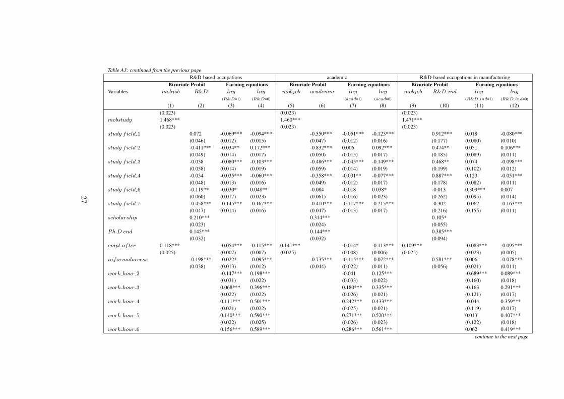
Table A3: continued from the previous pageR&D-based occupations academic R&D-based occupations in manufacturing

Bivariate Probit Earning equations Bivariate Probit Earning equations Bivariate Probit Earning equationsVariables mobjob R&D lny lny mobjob academia lny lny mobjob R&D ind lny lny

(R&D=1) (R&D=0) (acad=1) (acad=0) (R&D ind=1) (R&D ind=0)

(1) (2) (3) (4) (5) (6) (7) (8) (9) (10) (11) (12)(0.023) (0.023) (0.023)

mobstudy 1.468*** 1.460*** 1.471***(0.023) (0.023) (0.023)

study field 1 0.072 -0.069*** -0.094*** -0.550*** -0.051*** -0.123*** 0.912*** 0.018 -0.080***(0.046) (0.012) (0.015) (0.047) (0.012) (0.016) (0.177) (0.080) (0.010)

study field 2 -0.411*** -0.034** 0.172*** -0.832*** 0.006 0.092*** 0.474** 0.051 0.106***(0.049) (0.014) (0.017) (0.050) (0.015) (0.017) (0.185) (0.089) (0.011)

study field 3 -0.038 -0.080*** -0.103*** -0.486*** -0.045*** -0.149*** 0.468** 0.074 -0.098***(0.058) (0.014) (0.019) (0.059) (0.014) (0.019) (0.199) (0.102) (0.012)

study field 4 -0.034 -0.035*** -0.060*** -0.358*** -0.031** -0.077*** 0.887*** 0.123 -0.051***(0.048) (0.013) (0.016) (0.049) (0.012) (0.017) (0.178) (0.082) (0.011)

study field 6 -0.119** -0.030* 0.048** -0.084 -0.018 0.038* -0.013 0.309*** 0.007(0.060) (0.017) (0.023) (0.061) (0.016) (0.023) (0.262) (0.095) (0.014)

study field 7 -0.458*** -0.145*** -0.167*** -0.410*** -0.117*** -0.215*** -0.302 -0.062 -0.163***(0.047) (0.014) (0.016) (0.047) (0.013) (0.017) (0.216) (0.155) (0.011)

scholarship 0.210*** 0.314*** 0.105*(0.023) (0.024) (0.055)

Ph.D end 0.145*** 0.144*** 0.385***(0.032) (0.032) (0.094)

empl after 0.118*** -0.054*** -0.115*** 0.141*** -0.014* -0.113*** 0.109*** -0.083*** -0.095***(0.025) (0.007) (0.007) (0.025) (0.008) (0.006) (0.025) (0.023) (0.005)

informalaccess -0.198*** -0.022* -0.095*** -0.735*** -0.115*** -0.072*** 0.581*** 0.006 -0.078***(0.038) (0.013) (0.012) (0.044) (0.022) (0.011) (0.056) (0.021) (0.011)

work hour 2 -0.147*** 0.198*** -0.041 0.125*** -0.689*** 0.089***(0.031) (0.022) (0.033) (0.022) (0.160) (0.018)

work hour 3 0.068*** 0.396*** 0.180*** 0.335*** -0.163 0.291***(0.022) (0.022) (0.026) (0.021) (0.121) (0.017)

work hour 4 0.111*** 0.501*** 0.242*** 0.433*** -0.044 0.359***(0.021) (0.022) (0.025) (0.021) (0.119) (0.017)

work hour 5 0.140*** 0.590*** 0.271*** 0.520*** 0.013 0.407***(0.022) (0.025) (0.026) (0.023) (0.122) (0.018)

work hour 6 0.156*** 0.589*** 0.286*** 0.561*** 0.062 0.419***continue to the next page

27

Table A3: continued from the previous pageR&D-based occupations academic R&D-based occupations in manufacturing

Bivariate Probit Earning equations Bivariate Probit Earning equations Bivariate Probit Earning equationsVariables mobjob R&D lny lny mobjob academia lny lny mobjob R&D ind lny lny

(R&D=1) (R&D=0) (acad=1) (acad=0) (R&D ind=1) (R&D ind=0)

(1) (2) (3) (4) (5) (6) (7) (8) (9) (10) (11) (12)(0.024) (0.031) (0.028) (0.029) (0.186) (0.020)

Service -0.116*** -0.068*** -0.034*** -0.083***(0.011) (0.011) (0.009) (0.009)

Agriculture -0.149*** -0.089*** -0.087*** -0.109***(0.029) (0.029) (0.022) (0.023)

paper 2 0.606*** 0.611*** -0.053(0.035) (0.038) (0.062)

paper 3 1.357*** 1.346*** -0.354***(0.032) (0.035) (0.058)

monograph 2 0.170*** 0.279*** -0.315***(0.026) (0.025) (0.071)

monograph 3 0.161*** 0.348*** -0.231*(0.050) (0.049) (0.136)

patent 2 0.492*** 0.034 0.656***(0.048) (0.046) (0.063)

patent 3 0.565*** -0.266** 1.236***(0.126) (0.114) (0.132)

R&D GDP 43.342*** 2.848 134.706***(15.394) (15.520) (34.856)

crisis -0.240*** 0.020*** -0.106*** -0.093*** 0.025*** -0.101*** -0.538*** -0.032 -0.040***(0.028) (0.006) (0.007) (0.028) (0.006) (0.006) (0.068) (0.020) (0.005)

HSempl share 0.051*** 0.003*** 0.003*** 0.049*** 0.003*** 0.003*** 0.051*** 0.007*** 0.003***(0.002) (0.000) (0.001) (0.002) (0.001) (0.001) (0.002) (0.002) (0.000)

density -0.036** 0.008** 0.013*** -0.042** -0.006 0.014*** -0.039** 0.016 0.010***(0.018) (0.004) (0.005) (0.018) (0.004) (0.004) (0.018) (0.013) (0.003)

Constant -6.251*** -1.700*** 2.551*** 2.259*** -6.058*** -0.999*** 2.235*** 2.352*** -6.269*** -4.757*** 2.579*** 2.328***(0.234) (0.271) (0.058) (0.074) (0.233) (0.273) (0.064) (0.065) (0.234) (0.625) (0.310) (0.048)

Observations 18,640 18,640 8,629 10,010 18,640 18,640 7,215 11,424 18,640 18,640 551 18,088R-squared 0.155 0.385 0.174 0.371 0.334 0.280

⇢ -0.077 -0.212 0.082continue to the next page

28

Table A3: continued from the previous pageR&D-based occupations academic R&D-based occupations in manufacturing

Bivariate Probit Earning equations Bivariate Probit Earning equations Bivariate Probit Earning equationsVariables mobjob R&D lny lny mobjob academia lny lny mobjob R&D ind lny lny

(R&D=1) (R&D=0) (acad=1) (acad=0) (R&D ind=1) (R&D ind=0)

(1) (2) (3) (4) (5) (6) (7) (8) (9) (10) (11) (12)LR test of ⇢ = 0:chi2 (p-value) 26.597 (0.000) 188.922 (0.000) 6.878 (0.009)

Legend: all regressions include socio-demographic variables, Ph.D-related variables, job-related variables, Ph.D university provincial dummies, Ph.D university regional dummiesand constant. Standard errors (columns 1, 2, 5, 6, 9 and10)/Bootstrapped standard errors (columns 3, 4, 7, 8, 11 and 12) in parentheses. Significance is indicated as follows: ***denoting the 1%, ** the 5% and * the 10% level.

29

Table A4: Mobility-earning equation - double sample selection model. Only workers who work more than 26 hours per week

R&D-based occupations academic R&D-based occupations in manufacturingBivariate Probit Earning equations Bivariate Probit Earning equations Bivariate Probit Earning equations

Variables mobjob R&D lny lny mobjob academic lny lny mobjob R&D ind lny lny

(R&D=1) (R&D=0) (academic=1) (academic=0) (R&D ind=1) (R&D ind=0)(1) (2) (3) (4) (5) (6) (7) (8) (9) (10) (11) (12)

mobjob 0.011 0.039*** -0.047* 0.037*** 0.138** 0.031***(0.023) (0.014) (0.025) (0.013) (0.060) (0.011)

lambda mob 0.016* 0.014 0.024** 0.017** -0.070 0.022***(0.009) (0.009) (0.010) (0.008) (0.056) (0.007)

lambda occ 0.017* 0.015* 0.031*** -0.008 -0.012 0.000(0.010) (0.009) (0.011) (0.009) (0.015) (0.029)

visiting abroad 0.092*** 0.104*** 0.088***(0.025) (0.025) (0.025)

study mobility 1.422*** 1.411*** 1.425***(0.026) (0.025) (0.026)

papers 2 0.637*** 0.648*** -0.059(0.039) (0.042) (0.064)

papers 3 1.388*** 1.392*** -0.401***(0.035) (0.039) (0.060)

monograph 2 0.174*** 0.284*** -0.314***(0.029) (0.028) (0.073)

monograph 3 0.171*** 0.319*** -0.322**(0.056) (0.055) (0.150)

patent 2 0.457*** -0.000 0.643***(0.050) (0.048) (0.065)

patent 3 0.561*** -0.351*** 1.265***(0.136) (0.121) (0.135)

R&D GDP 50.760*** 8.367 128.674***(16.809) (16.920) (36.136)

Observations 15,412 15,412 7,968 7,443 15,412 15,412 6,484 8,927 15,412 15,412 533 14,878R-squared 0.119 0.314 0.092 0.292 0.260 0.200LR test of ⇢ = 0 (p-value)

Legend: all regressions include socio-demographic variables, Ph.D-related variables, job-related variables, Ph.D university provincial dummies,Ph.D university regional dummies and constant. Standard errors (columns 1, 2, 5, 6, 9 and10)/Bootstrapped standard errors (columns 3,4, 7, 8, 11 and 12) in parentheses. Significance is indicated as follows: *** denoting the 1%, ** the 5% and * the 10% level.

30

Table A5: Mobility-earning equation - double sample selection model. Only Ph.D holders who started working after doctoral degree

R&D-based occupations academic R&D-based occupations in manufacturingBivariate Probit Earning equations Bivariate Probit Earning equations Bivariate Probit Earning equations

Variables mobjob R&D lny lny mobjob academic lny lny mobjob R&D ind lny lny

(R&D=1) (R&D=0) (academic=1) (academic=0) (R&D ind=1) (R&D ind=0)(1) (2) (3) (4) (5) (6) (7) (8) (9) (10) (11) (12)

mobjob -0.034 0.044*** -0.085** 0.033** 0.144* 0.028**(0.026) (0.016) (0.033) (0.014) (0.084) (0.012)

lambda mob 0.030*** 0.013 0.039*** 0.027*** -0.086 0.021***(0.009) (0.011) (0.012) (0.009) (0.103) (0.007)

lambda occ 0.032*** 0.005 0.044*** -0.028*** -0.011 -0.010(0.012) (0.011) (0.014) (0.011) (0.021) (0.035)

visiting abroad 0.104*** 0.115*** 0.100***(0.027) (0.027) (0.027)

study mobility 1.408*** 1.399*** 1.411***(0.028) (0.028) (0.028)

papers 2 0.636*** 0.698*** -0.059(0.042) (0.046) (0.072)

papers 3 1.354*** 1.416*** -0.361***(0.039) (0.043) (0.067)

monograph 2 0.184*** 0.308*** -0.346***(0.031) (0.030) (0.084)

monograph 3 0.151** 0.372*** -0.106(0.061) (0.061) (0.150)

patent 2 0.379*** 0.008 0.591***(0.056) (0.053) (0.074)

patent 3 0.489*** -0.169 0.974***(0.156) (0.140) (0.174)

R&D GDP 36.313** -0.423 157.667***(18.014) (18.144) (39.868)

Observations 13,062 13,062 6,671 6,390 13,062 13,062 5,711 7,350 13,062 13,062 419 12,642R-squared 0.144 0.354 0.166 0.350 0.316 0.253LR test of ⇢ = 0 (p-value)

Legend: all regressions include socio-demographic variables, Ph.D-related variables, job-related variables, Ph.D university provincial dummies,Ph.D university regional dummies and constant. Standard errors (columns 1, 2, 5, 6, 9 and10)/Bootstrapped standard errors (columns 3,4, 7, 8, 11 and 12) in parentheses. Significance is indicated as follows: *** denoting the 1%, ** the 5% and * the 10% level.

31

Table A6: Mobility-earning equation - double sample selection model. Only STEM (Science, Technology, Engineering and Mathemat-ics) fields of study

R&D-based occupations academic R&D-based occupations in manufacturingBivariate Probit Earning equations Bivariate Probit Earning equations Bivariate Probit Earning equations

Variables mobjob R&D lny lny mobjob academic lny lny mobjob R&D ind lny lny

(R&D=1) (R&D=0) (academic=1) (academic=0) (R&D ind=1) (R&D ind=0)(1) (2) (3) (4) (5) (6) (7) (8) (9) (10) (11) (12)

mobjob -0.018 0.067*** -0.144*** 0.042*** 0.149* 0.034***(0.024) (0.018) (0.036) (0.015) (0.078) (0.013)

lambda mob 0.034*** 0.001 0.054*** 0.029*** -0.058 0.019**(0.009) (0.012) (0.015) (0.009) (0.060) (0.008)

lambda occ 0.027** -0.019 0.065*** -0.063*** -0.019 0.009(0.012) (0.012) (0.014) (0.012) (0.021) (0.030)

visiting abroad 0.059* 0.064** 0.052(0.032) (0.032) (0.032)

study mobility 1.316*** 1.298*** 1.322***(0.034) (0.033) (0.034)

paper 2 0.555*** 0.587*** -0.059(0.047) (0.054) (0.068)

paper 3 1.392*** 1.370*** -0.387***(0.042) (0.049) (0.063)

monograph 2 0.135*** 0.221*** -0.336***(0.040) (0.039) (0.082)

monograph 3 0.102 0.271*** -0.302*(0.083) (0.078) (0.167)

patent 2 0.420*** 0.005 0.656***(0.054) (0.052) (0.068)

patent 3 0.729*** -0.333*** 1.313***(0.153) (0.128) (0.138)

R&D GDP 22.260 -10.732 131.292***(20.992) (21.114) (37.795)

Observations 9,715 9,715 5,185 4,530 9,715 9,715 3,760 5,955 9,715 9,715 486 9,229R-squared 0.159 0.329 0.136 0.326 0.338 0.234LR test of ⇢ = 0 (p-value)

Legend: all regressions include socio-demographic variables, Ph.D-related variables, job-related variables, Ph.D university provincial dummies,Ph.D university regional dummies and constant. Standard errors (columns 1, 2, 5, 6, 9 and 10)/Bootstrapped standard errors (columns 3,4, 7, 8, 11 and 12) in parentheses. Significance is indicated as follows: *** denoting the 1%, ** the 5% and * the 10% level.

32

References

Abreu, M., A. Faggian, and P. McCann (2015). Migration and inter-industry mobility of ukgraduates. Journal of Economic Geography 15(2), 353–385.

Agarwal, R. and A. Ohyama (2013). Industry or academia, basic or applied? career choices andearnings trajectories of scientists. Management Science 59(4), 950–970.

Aghion, P., M. Dewatripont, and J. C. Stein (2008). Academic freedom, private-sector focus,and the process of innovation. The RAND Journal of Economics 39(3), 617–635.

Aldashev, A., J. Gernandt, and S. L. Thomsen (2009). Language usage, participation, em-ployment and earnings: Evidence for foreigners in west germany with multiple sources ofselection. Labour Economics 16(3), 330–341.

Axelsson, R. and O. Westerlund (1998). A panel study of migration, self-selection and householdreal income. Journal of Population Economics 11(1), 113–126.

Azoulay, P., I. Ganguli, and J. Graff Zivin (2017). The mobility of elite life scientists: Profes-sional and personaldeterminants. Research Policy, 573–590.

Ballarino, G. and S. Colombo (2010). Occupational outcomes of phd graduates in northern italy.Italian Journal of Sociology of Education 2(2).

Bender, K. A. and J. S. Heywood (2006). Job satisfaction of the highly educated: The role ofgender, academic tenure, and earnings. Scottish Journal of Political Economy 53(2), 253–279.

Bender, K. A. and J. S. Heywood (2009). Educational mismatch among ph. ds: determinantsand consequences. In Science and engineering careers in the United States: An analysis ofmarkets and employment, pp. 229–255. University of Chicago Press.

Bloch, C., E. K. Graversen, and H. S. Pedersen (2015). Researcher mobility and sector careerchoices among doctorate holders. Research Evaluation 24(2), 171–180.

Bonnard, C. (2012). The access of the young graduates in sciences into r&d profession: Aswitching model treatment for the french case. Labour 26(1), 46–65.

Borjas, G. J., S. G. Bronars, and S. J. Trejo (1992). Self-selection and internal migration in theunited states. Journal of Urban Economics 32(2), 159–185.

Buchel, F. and M. Van Ham (2003). Overeducation, regional labor markets, and spatial flexibil-ity. Journal of Urban Economics 53(3), 482–493.

Campostrini, S. (2011). After the phd: A study of career paths, job and training satisfactionamong phd graduates from an italian university. In Statistical Methods for the Evaluation ofUniversity Systems, pp. 209–222. Springer.

Causa, O. and A. Johansson (2011). Intergenerational social mobility in oecd countries. OECDJournal: Economic Studies 2010/1(6), 1–44.

33

Checchi, D. (2010). Immobilita diffusa. Perche la mobilita intergenerazionale e cosı bassa inItalia. Il Mulino.

Chiswick, B. R. and P. W. Miller (2009). The international transferability of immigrants’ humancapital. Economics of Education Review 28(2), 162–169.

Coniglio, N. D. and F. Prota (2008). Human capital accumulation and migration in a peripheraleu region: the case of basilicata. Papers in Regional Science 87(1), 77–95.

Conti, A. and F. Visentin (2015). A revealed preference analysis of phd students? choices overemployment outcomes. Research Policy 44(10), 1931–1947.

Cutillo, A. and C. Ceccarelli (2012). The internal relocation premium: are migrants positivelyor negatively selected? evidence from italy. Journal of Applied Statistics 39(6), 1263–1278.

DaVanzo, J. (1983). Repeat migration in the united states: who moves back and who moves on?The Review of Economics and Statistics, 552–559.

Detang-Dessendre, C., C. Drapier, and H. Jayet (2004). The impact of migration on wages:empirical evidence from french youth. Journal of Regional Science 44(4), 661–691.

Devillanova, C. (2013). Over-education and spatial flexibility: New evidence from italian surveydata. Papers in Regional Science 92(3), 445–464.

Di Cintio, M. and E. Grassi (2013). Internal migration and wages of italian university graduates.Papers in Regional Science 92(1), 119–140.

Di Cintio, M. and E. Grassi (2016). International mobility and wages: An analysis of ItalianPh.D. graduates. The Annals of Regional Science, 1–33.

Di Paolo, A. (2011). Knowledge of catalan, public/private sector choice and earnings: Evidencefrom a double sample selection model. Hacienda Publica Espanola /Revista de economiapublica 197(2), 9–35.

Di Paolo, A. (2016). (endogenous) occupational choices and job satisfaction among recentspanish phd recipients. International Journal of Manpower 37(3), 511–535.

Di Paolo, A. and F. Mane (2016). Misusing our talent? overeducation, overskilling and skillunderutilisation among spanish phd graduates. The Economic and Labour Relations Re-view 27(4), 432–452.

Ermini, B., L. Papi, and F. Scaturro (2017). An analysis of the determinants of over-educationamong italian ph.d graduates. Italian Economic Journal, forthcoming, 1–41.

Faggian, A. and P. McCann (2009). Universities, agglomerations and graduate human capitalmobility. Tijdschrift voor economische en sociale geografie 100(2), 210–223.

Fasola, S., O. Giambalvo, and C. Romano (2016). Flexible latent trait aggregation to analyzeemployability after the ph. d. in italy. Journal of Applied Statistics 43(1), 180–194.

34

Friedberg, R. M. (2000). You can’t take it with you? immigrant assimilation and the portabilityof human capital. Journal of labor economics 18(2), 221–251.

Gaeta, G. L. (2015a). Was it worth it? an empirical analysis of over-education among ph.d.recipients in italy. International Journal of Social Economics 42(3).

Gaeta, G. L. (2015b). Was it worth it? An empirical analysis of over-education among Ph.D.recipients in Italy. International Journal of Social Economics 42(3).

Gottlieb, P. D. and G. Joseph (2006). College-to-work migration of technology graduates andholders of doctorates within the united states. Journal of Regional Science 46(4), 627–659.

Goux, D. and E. Maurin (2000). Returns to firm-provided training: evidence from frenchworker–firm matched data. Labour economics 7(1), 1–19.

Greenwood, M. J. (1997). Internal migration in developed countries. Handbook of populationand family economics 1, 647–720.

Haapanen, M. and H. Tervo (2012). Migration of the highly educated: Evidence from residencespells of university graduates. Journal of Regional Science 52(4), 587–605.

Ham, J. C., X. Li, and P. B. Reagan (2011). Matching and semi-parametric iv estimation, adistance-based measure of migration, and the wages of young men. Journal of Economet-rics 161(2), 208–227.

Heckman, J. (1979). Sample selection bias as a specification error. Econometrica, 153–161.

Heitmueller, A. (2006). Public-private sector pay differentials in a devolved scotland. Journalof Applied Economics 9(2), 295.

Hensen, M. M., M. R. De Vries, and F. Corvers (2009). The role of geographic mobility inreducing education-job mismatches in the netherlands. Papers in Regional Science 88(3),667–682.

Herzog, H. W., A. M. Schlottmann, and T. P. Boehm (1993). Migration as spatial job–search: asurvey of empirical findings. Regional Studies 27(4), 327–340.

Herzog, H. W., A. M. Schlottmann, and D. L. Johnson (1986). High-technology jobs and workermobility. Journal of Regional Science 26(3), 445–459.

Iammarino, S. and E. Marinelli (2015). Education–job (mis) match and interregional migration:Italian university graduates’ transition to work. Regional Studies 49(5), 866–882.

Jauhiainen, S. (2011). Overeducation in the finnish regional labour markets. Papers in RegionalScience 90(3), 573–588.

Lee, L.-F. (1978). Unionism and wage rates: A simultaneous equations model with qualitativeand limited dependent variables. International economic review, 415–433.

35

Lehmer, F. and J. Ludsteck (2011). The returns to job mobility and inter-regional migration:Evidence from germany. Papers in Regional Science 90(3), 549–571.

Lehmer, F. and J. Moller (2008). Group-specific effects of inter-regional mobility on earnings–amicrodata analysis for germany. Regional Studies 42(5), 657–674.

Lemistre, P. and N. Moreau (2009). Spatial mobility and returns to education: some evidencefrom a sample of french youth. Journal of Regional Science 49(1), 149–176.

Lkhagvasuren, D. (2014). Education, mobility and the college wage premium. European Eco-nomic Review 67, 159–173.

Mangematin, V. (2000). Phd job market: professional trajectories and incentives during the phd.Research policy 29(6), 741–756.

Mohanty, M. S. (2001). Determination of participation decision, hiring decision, and wages in adouble selection framework: Male-female wage differential in the us labor market revisited.Contemporary Economic Policy 19(2), 197.

Nakosteen, R. A. and O. Westerlund (2004). The effects of regional migration on gross incomeof labour in sweden. Papers in Regional Science 83(3), 581–595.

Nakosteen, R. A., O. Westerlund, and M. Zimmer (2008). Migration and self-selection: Meas-ured earnings and latent characteristics. Journal of Regional Science 48(4), 769–788.

Nakosteen, R. A. and M. Zimmer (1980). Migration and income: the question of self-selection.Southern Economic Journal, 840–851.

Nakosteen, R. A. and M. Zimmer (1982). The effects on earnings of interregional and interin-dustry migration. Journal of Regional Science 22(3), 325–341.

Naldini, M. and T. Jurado (2013). Family and welfare state reorientation in spain and inertia initaly from a european perspective. Population Review 52(1).

Pedersen, H. S. (2016). Are phds winners or losers? wage premiums for doctoral degrees inprivate sector employment. Higher Education 71(2), 269–287.

Pekkala, S. (2002). Migration and individual earnings in finland: a regional perspective. Re-gional Studies 36(1), 13–24.

Roach, M. and H. Sauermann (2010). A taste for science? phd scientists’ academic orientationand self-selection into research careers in industry. Research Policy 39(3), 422–434.

Rodrıguez-Pose, A. and V. Tselios (2010). Returns to migration, education and externalities inthe european union. Papers in Regional Science 89(2), 411–434.

Sauermann, H. and M. Roach (2012). Taste for science, taste for commercialization, and hybridscientists. Organisation, Economics and Policy of Scientific Research, Torino, Italy.

36

Sjaastad, L. A. (1962). The costs and returns of human migration. Journal of political Eco-nomy 70(5, Part 2), 80–93.

Stern, S. (2004). Do scientists pay to be scientists? Management science 50(6), 835–853.

Tunali, I. (1986). A general structure for models of double-selection and an application to ajoint migration/earnings process with remigration. Research in labor Economics 8(Part B),235–282.

Yankow, J. J. (2003). Migration, job change, and wage growth: a new perspective on the pecu-niary return to geographic mobility. Journal of Regional Science 43(3), 483–516.

37