1

Wage differentials and gender discrimination –changes in Sweden 1981-1998

Mats Johansson*Katarina Katz **Håkan Nyman***

AbstractThe purpose of this paper is to follow the development of the Swedish gender earnings gapthrough the 1980s and 1990s. We follow the changes in the wage gap and in factors to whichit can be related, step-by-step, and year-by-year. This is done by analysing cross sectionaldata from statistics Sweden (HINK) for the years 1981, 1983-1991 and 1993-1998. Thepreliminary results show that the unadjusted wage gap varied between 15-20 percent up to1989 when the differentials began to increase. During the 90s the size of the gap was around25 percent. There is an increase in the wage differentials between the 1980s and late 1990s. Ina decomposition analysis we find that the measured differences in jobs and qualificationsbetween women and men can account only for between two and three fifths of the genderwage gap, if they are assumed to be rewarded according to the wage function for men. If thefemale wage function is applied, considerably less of the differentials are explained.Differences in the educational requirements for jobs have contributed considerably to genderearnings inequality. The impact has, however, decreased over the period studied and is abouthalf as large in the 1990s as it was in the 1980s.

JEL Classification: J16, J31, J71Keywords: Gender differentials, wage differentiation, Swedish labour market, discrimination

* Institute for Futures Studies, Stockholm, mats.johansson@framtidsstudier.se** Department of Economics, Stockholm University, kk@ne.su.se*** National Insurance Board, Stockholm, hakan.nyman@rfv.se

2

1. IntroductionThe purpose of this paper is to follow the development of the Swedish gender earnings gap

through the 1980s and 1990s. In the course of these two decades, very significant changes

with strong impact on the wage setting process took place in Sweden. The most conspicuous

alteration is the increase in overall income and earnings differentiation in a country, which for

a long time was know as one of the least unegalitarian in this respect. It has been forcefully

argued, in international comparisons, that the greater the total spread in earnings, the larger

the gender gap (Blau and Kahn 1992). It may therefore be more than a coincidence that an

increase in earnings differentiation and a halt in the trend towards gender earnings equality

have occurred simultaneously in Sweden.

Behind, or concomitant with, the increase in differentiation are a whole series of institutional

and economic changes, such as the disintegration of the system of centralised wage

bargaining, the income tax reform of the early 90s, the boom of the 1980s, which was

followed in 1992-97 by a downturn with levels of unemployment unseen since the Great

Depression, Swedish entry into the European Union, the currency crises of 1992 and strong

fiscal pressure against public sector activities.

In this context of manifold events, we want to not just compare a certain point in time at the

beginning of this period with another at the end of it. We want to follow the changes in the

wage gap, and in factors to which it can be related, step-by-step, and year-by-year. We do this

by analysing data from repeated cross section surveys from Statistics Sweden (the HINK-

database) for the years 1981, 1983-1991 and 1993-1998. This data set will be discussed in

more detail below (section 4), but it can be said at the outset that we consider the quality of

sampling and interviewing etceteras, to be good. The problems with the data set are due, first,

to the fact that it was not created for the purpose of wage-analysis and, second, that some

questions and, thus, some variables have changed over the almost twenty years that the survey

has been conducted. Therefore we have had to use proxies for, or approximations of, some

important variables, because this was the best that the data permitted or to ensure

commensurability over time. To some extent, this is always the case in empirical analysis

covering a long time span. Any data including different points in time would have to take into

account, and make imputations to correct for, institutional changes, which necessitate changes

in definition and interpretation of variables.

3

We consider, however, that to have this rich time-series, enables us to make a unique

contribution which should be seen as a complement, not an alternative, to studies based on

data sets which include other variables but not such a continuous development over time.

2. Theories

Attempts at explanation of inequality in earnings between women and men have traditionally

emphasised a number of interrelated explanatory mechanisms. Some of these mechanisms are

briefly described below. (For a more extensive discussion, see Katz, 1994, 2001.)

Economists distinguish two main types of explanation: “Pure” wage discrimination, which

means that women are paid less than equally productive men are. In neo-classical theory, this

discrimination is explained by “preferences for discrimination” on the part of employers, co-

workers or customers. If these preferences are not equally strong everywhere, in the long run,

discrimination would tend to be replaced by segregation (Becker, 1971, Cain, 1986).

The second line of argument is that women are paid less by profit-maximising employers

because they are less productive. Obviously, both things could be true, simultaneously and

explain parts of the gender gap in wages. Also, the reasons for the assumed lower productivity

of women include other forms of discrimination, both inside the labour market (in hiring, on-

the-job-training and promotion) and outside it (in households or education). The argument

may be made both in terms of the individual woman’s productivity and corresponding wage

and of employers paying all women according to the average productivity of female workers

(statistical discrimination).

According to some economists, because of the division of labour (specialisation) in the

household women have weaker labour market attachment and less incentive to invest time

and effort on education and careers. Since women often take more responsibility for family

and household work, women’s labour force participation is often interrupted and women more

often work part time (Mincer and Polachek 1974; Polachek 1981; Becker 1985). This would

imply that women generally accumulate less education; job training and work experience

compared to men and are hence, less productive and less paid. In particular, if women expect

to make career breaks, they may prefer occupations with higher starting wages but lower

4

returns to experience (wage growth) in order to minimise the loss from temporary absence

(Polachek, 1981, Kim and Polachek, 1994). This hypothesis is, however, disputed. England et

al. (1988) estimate an earnings model with fixed (time- and individual-) effects on US panel

data to investigate the relationship between earnings and sex composition of occupations, for

black and white men and women. They find significant negative effects of percentage female

in the occupation on starting wages, for full-time workers in all four race/gender groups.

Thus, women do not appear to choose job with higher starting wages. England (1982) tests for

a relationship between sex composition, on the one hand, and rewards to experience or

"penalties" for post-school years spent out of the labour force, on the other and finds that

women do not maximise lifetime earnings by working in traditionally female occupations.

The theory of compensating differentials predicts that wages will be lower in jobs with more

desirable working conditions1. It is feasible that men receive a higher wage as a compensation

for more unattractive working conditions. According to Filer (1985), because of different

tastes, men and women on the average choose occupations with different characteristics.

Daymont and Andrisani (1984) found that the values and preferences expressed by young

men were conducive to higher wages than those more common among young women. In this

case, there appears to be a “compensation” also for attractive features of male dominated jobs.

Sociologists often emphasise the effects of job segregation. According to this explanation

women tend to hold less advantageous work positions and to be employed within less

favourable work structures than men, regardless of intrinsic or potential productivity. Thus,

job segregation by sex is, in this sense, the main source of gender differences in labour market

out-comes. In the terminology of economic theory, job rationing allows discriminatory sorting

of women and men into branches and firms with different levels of productivity. Historical

and sociological studies find underestimation of the value and skill content of occupations

perceived as “female” (Walby, 1988, Phillips & Taylor, 1980).

Both the returns to skills and the size of the premium for employment in particular industries

have a potentially important role in the determination of the gender pay gap. (See e.g. Blau

and Kahn, 1999.) All else equal, the larger the returns to skills and the larger the rents

received by individuals in favoured industries, the larger the gender gap will be. Similarly,

1 See Rosen (1986).

5

labour market discrimination and/or actual female deficits in unmeasured skills result in

employers treating women as if they had lower unmeasured as well as measured skills. Thus,

the higher the rewards to unmeasured skills, the larger the gender gap, after controlling for

measured characteristics

The distinction between wage differences due to (different kinds of) discrimination and

productivity related differentials is complicated by endogeneity or feedback effects. For

instance, if women expect not to be paid according to their “human capital” they may choose

to acquire less than they would have in the absence of discrimination.

3. Background and Previous Studies

The Swedish labour market is characterised by a high level of unionisation. Both the strong

legal standing of the collective bargain and the strength of Swedish trade unions (including

white-collared) and employer organisations make collective bargaining a central instrument

for labour market regulation. Since the eighties there has been a general tendency to

decentralise wage bargaining and contracts to the branch, and even to the firm, level. This

tendency to decentralisation of the bargaining process has not been limited to wage

bargaining but also concerned working time arrangements. Trade union membership in

Sweden has risen constantly since the mid-1960s even though the union density experienced a

weak decline in connection with the sharp increase of unemployment in the early 1990:s.

3.1 Women’s position in the labour market

The Swedish gender earnings gap was significantly reduced between the 60’s and the early

80’s. However, since the mid 80’s the reduction in wage inequality has been halted. One

explanation for the improved situation of Swedish women is the compression of the overall

wage structure. This particularly favoured women who often had wages in the lower deciles

of the distribution. Another explanation behind the increasing relative wages for women prior

to the early 1980’s was the interplay of wage policy and demand/supply factors, which raised

the price of unskilled work, a large proportion of which was performed by women. A number

of political reforms strengthened women’s labour market attachment. Concerning direct legal

regulation of equal pay, Sweden as late as 1980 enforced an anti discrimination law.

6

However, such regulation had in practice been enforced in the early 70’s through collective

bargaining.

The expansion of the educational system seems to have improved women’s position in the

labour market. Since, the mid 70’s the rate of enrolment in education of young women (20-24

years of age) has exceeded that of men, and it has increased over time. Separate taxation of

spouse was introduced in 1971 and, in conjunction with the progressive rates of taxation in

force until 1991, had a strong effect on the labour force participation of married women

(Gustafsson and Bruyn-Hundt, 1991). Subsidised child-care and a generous parental leave

system, relative to most countries, are important means for young women to retain their

labour force attachment and human capital accumulation, compared to leaving employment in

order to care for young children Gustafsson and Stafford, 1992). The work experience

foregone, as well as perceived depreciation of skills, during parental leave does, however,

have a considerable negative impact on wages (Albrecht et. al., 1997). A hypothetical

situation without employment breaks or with parental leave equally shared between parents

would result in a smaller gender wage gap.

3.2 Previous studies

Most studies of the Swedish gender wage gap focus on the 80:s and early 90:s. The most

frequently used data source is the Level of Living Survey (LNU), which covers the years

1968, 1981, 1991 and 2000. Another is the HUS panel. The 1984, 1986, 1993 waves of HUS

have been used for such studies.

A study by Löfström (1989) – using HUS 1984 - finds that the female/male wage ratio would

have been 15-25 percentage points higher in the absence of gender wage discrimination.

Among other thing she finds that returns of education and to work experience are lower for

women than for men. Andersson (1995) analyses HUS data for the years 1984, 1986 and

1993. He finds that the wage offer gap2 increased over the years, and so did the amount which

can be ascribed to discrimination3, but not to the same extent. In 1984 the male-female log

wage gap was 21 percentage points of which market discrimination accounted for 13

2 The wage gap corrected for selectivity, see section 4 below.3 The method of decomposing wage differentials into one part attributable to characteristics and one ascribable todiscrimination is described in section 4, below.

7

percentage points (or 60 % of the gap). In other words, according to his wage-model,

women’s wages would have been on average 13 percentage points higher on average in the

absence of discrimination. In 1986 this had increased slightly, while in 1993 the log wage gap

had increased to 23 percentage points, discrimination to 19 percentage points (81 % of the

gap). In separate analysis of wages in the public and private sectors, Andersson finds that the

log wage offer gap was 27 percentage points (19 % of which was discrimination) in the

private and 20 percentage points (15 % discrimination) in the public sector. In a further

decomposition of the productivity differentials, human capital variables turned out to be the

most important. Trying to trace compensating wage differentials, he finds that most of the

estimated parameters for undesirable job characteristics had negative signs, except for "shift

work".

Studying LNU data for 1981, le Grand (1991) finds that human capital and family obligation

explanations for the gender pay gap account for about 30 percent of the total gap. According

to his calculations, human capital variables explain approximately one-fifth of the gender pay

gap. However, job segregation seems to be the most important explanatory factor in the

model. Compensating wage differentials cannot be shown to make any significant

contribution to the gender pay gap. In a cross section analysis on LNU -81, -91 Le Grand

(1997) shows that the correlation between occupational segregation and wage does not

depend on female occupations being more compatible with housework and family obligation.

However, employees in male dominated occupations receive on average more on the job

training. According to le Grand the correlation between the gender composition in the

occupation and the wage can be explained by skill requirements, on the job training,

management responsibility, social class and sector.

Taking into account the explanations mentioned above there remains a wage effect due to the

proportion of women in the occupation, which cannot be explained by other variables. This

net wage effect -- which le Grand interprets as the lowest possible level for the valuation of

wage discrimination -- implies that women employed in a male dominated occupation (at

least 90 per cent men) receive at least 9 per cent more per hour compared to women in female

dominated occupations (90 per cent women). The corresponding difference for men is 6 per

cent. With a model that does not control for social class and occupational segregation, the

wage difference between male and female dominated occupations is 14 per cent for women

and 10 per cent for men.

8

Palme and Wright (1992) test the hypothesis that there is a compensating wage differential

associated with undesirable job characteristics, using LNU 1981. Generally, they find no

evidence that the unexplained gender wage differences are associated with undesirable job

attributes.

Edin and Richardsson (1999) investigate the role of wage compression for the gender gap in

Sweden during the period 1968-1991 (using LNU data) and find that the effects of change in

the wage structure on women’s wages have varied over time and have partly counteracting

effects. According to Edin and Richardsson, changes in the wage structure were particularly

important up to the mid 70’s, but in 1981 the wage compression effect accounted only for a

minor proportion of women’s relative wage gains, compared to the mid 70’s. The small

increase in the gender wage gap between 1981 and 1991 seemed according to Edin and

Richardsson be driven by changed inter-industry wage differentials.

Arai and Thoursie (1997) finds that there are systematic, gender specific wage differentials,

i.e. women earn less than men both across and - even more so - within occupations, and that

these wage differentials cannot be explained by observed personal background characteristics,

or by individual productivity-related or job-related characteristics. If women were distributed

over occupational groups in the same way as men are, their share would fall noticeably in

"health and social work", "financial and office-technical work" and "services". On the other

hand, the female share would increase considerably in "manufacturing" and in "technical and

medical work, etc. "

According to Arai and Thoursie, if women chose or were selected into occupational groups in

the same way as men, the female share would increase considerably in the category "blue-

collar, skilled". The female share would also increase in the category "white-collar high level"

but would fall in "blue-collar, unskilled" and in "white-collar, unqualified". According to the

segregation indices, the differences in men and women's occupational choices cannot be

explained to any great extent by level of education.

Using register data from employers, Meyerson and Petersen (1997) study the gender wage

gap for women and men at the same work establishment and with similar duties and level of

position. They show that the total gender pay gap in 1990 was on average 12.8 percent for

9

blue-collar workers and 27.8 for white-collar workers. According to their analysis the total

gender wage gap increased by 1.5 per cent between 1970 and 1990, while the gap for white-

collar workers declined during the period.

le Grand, Szulkin and Thålin (2001) follow changes in the Swedish wage structure through

the LNU. As Edin and Richardsson (ibid.), they find that the gender wage gap, both

unadjusted and adjusted for education and experience, decreased in the periods 1968-74 and

1974-81, particularly in the former, while it remained virtually constant 1981-91. The latest

wave of LNU, indicates that from 1991 to 2000 there was a slight decrease in the unadjusted

gap and a slight increase in the adjusted. le Grand, Szulkin and Thålin conclude that the most

important factors behind the decrease in the gender gap 1968-81 were an improvement in the

relative position of women compared to men in the same education and experience-categories

and, particularly during the first period, decreased wage differentiation within these

categories. Conversely, the convergence between men and women in terms of education and

experience after 1981 has not resulted in a commensurate convergence in wages, mainly

because wage differentiation, given education and experience, has grown.

le Grand, Szulkin and Thålin note that the adjusted gender wage gap was larger in the private

than in the public sector. In the first three waves of LNU women earned more in the public

than in the private sector, given education and experience. In 1991 and 2000 they earned more

in the private sector.

4. Empirical model

In order to examine determinants of female and male wages, cross-sectional wage equations

are estimated for the years 1981-1991 and 1993-1998. The first step is to estimate wage

equations separately for women and men. The hourly wage of individual i may be written as

iMii eXW += βln [1]

if i is male and as

iFii eXW += βln [2]

10

if i is female. The subscripts M and F indicate that the parameter refers to male and female,

respectively. lnWi is the natural logarithm of the hourly wage, Xi is a vector of variables

believed to determine earnings and e is an error term with zero mean and normal distribution.

It is common to refine the wage equation by using Heckman’s (1979) correction for sample

selection bias. In this case, a reduced-form probit equation of the probability of having any

observed wage (i.e. of Wi being greater than zero) is estimated and used for the construction

of the so-called Mills ratio, the inverse of which ("Heckman's lambda") is introduced into the

wage equation. The reason for the correction is that if the probability of being employed is

correlated with unobserved capacity to earn, the error term in the wage equation will be

correlated with wages. The distribution of observed wages will differ from the distribution of

"offered wages", which also include the potential wages of those who are not employed and

parameter estimates will be biased.

A correction was done in the present study, with a selection equation including dummies for

age categories, citizenship, marital status, presence of children in different age intervals,

regional (county level) unemployment rate and a variable indicating whether the individual is

entitled to disability benefits. The inverse of the Mill's ratio was significant in the wage

equation for women in six years out of 16, but only in two years for men. In addition, the

parameter for lambda in the male equations was negative in all but two cases (and in these it

was not significant). Because of this, and of the well-known difficulty of specifying the

selection equation correctly, we concluded that with the restrictive filters we had applied,

selectivity in employment did not significantly affect our results and that it was better to omit

the attempt at correction.

In this paper we will decompose the gender wage differential, following the standard method

of Oaxaca (1973). Since residuals are assumed to have zero mean, the difference between the

average log wages for men and women is:

)ˆˆ()ln(ln FFMMFM XXWW ββ −=− [3]

11

where hats (^) denote parameter estimates (estimated by OLS) and bars (-) indicate mean

values.

Assuming that a non-discriminatory wage structure, β*, is known it is possible to rewrite [3]

as:

*)()ˆ*(*)ˆ()ln(ln βββββ FMFFMMFM XXXXWW −+−+−=− [4]

The terms *)ˆ( ββ −MMX and )ˆ*( FFX ββ − on the right hand side in [4] may be interpreted

as possible discrimination. These terms represent the amount by which men’s and women’s

pay, respectively, differ from the assumed non-discriminatory wage. The third term,

*)( βFM XX − , represents difference in average characteristics between men and women

weighted by the non-discriminatory rate of return.

There are several ways of constructing the assumed non-discriminatory wage structure, β*. It

may be defined by a weighting matrix, as:

FM I βββ ˆ)(ˆ* Ω−+Ω= [5]

where Ω is a weighting matrix and I is the identity matrix.

Setting Ω=I implies that β*= Mβ and equation [4] becomes

MFMFMFFM XXXWW βββ ˆ)()ˆˆ()ln(ln −+−=−

With the opposite assumption, Ω=0, and β*= Fβ . Equation [4] becomes

FFMFMMFM XXXWW βββ ˆ)()ˆˆ()ln(ln −+−=− [7]

In [6] the male wage function is treated as the true representation of the relationship between

characteristics and productivity, while the female function is assumed true in [7]. The last

12

term in each of equations [4], [6] and [7] are called “the endowment term” or “the explained

part” because they indicate the part of the wage gap which can be attributed to measured

differences in characteristics (endowments). The remainder represents the part, which cannot

be explained by the variables included in the wage model, and is sometimes referred to as

“the discrimination term”,

Another possibility, as in Oaxaca and Ransom (1994) is to use Ω= )'()'( 1MM XXXX − . This

produces a β* equal to the OLS-estimate that would be obtained from estimating the wage-

equation on the pooled sample of men and women.

5. Data and definitions

5.1 Data

The Swedish Household Income Survey (HINK) is a survey tailored to the study of income

distribution in Sweden, and has been conducted annually since the mid 70s. The reference

population consists of all persons living in Sweden at least half of the calendar year. Survey

data is collected through telephone interviews, but also from administrative registers and tax

return forms. Both the selected respondent (“the sampling person”), who has to be of age 18

or older, and his/her household, are included in the survey. HINK includes 10 000 – 18 000

households annually.

The survey is rich in variables concerning income, transfers and taxes. There are many

background-variables as well as, for example, the industry a person is working in, occupation,

region of residence and marital status. These characteristics, i.e. a relatively large sample, the

richness of variables and the fact that the survey is conducted annually, make it suitable to use

HINK to investigate the male-female wage gap in Sweden.

From HINK, we have drawn a sub-sample, consisting of respondents (“the sampling

persons”, not the other members of their households) 20-64 years of age, reporting any labour

related income. We have excluded self-employed, farmers and full-time students as well as

agricultural workers and persons working in forestry and fishing. In addition, observations

13

with missing values for any variables used in the models are deleted. This has left us with data

sets including between 3400 and 5600 individuals each year.4

5.2 Choice of model

The variables used in the wage equations are: age, age squared, dummy variables for level of

education, for being a blue- or white-collar worker, industry, region, for being employed in

central government, local government or in the private sector, citizenship, share women in

occupation. (For exact definitions, see Table A1.) As HINK is a stratified data set, where the

stratification has been changed several times during the period of study, we have used weights

when estimating mean values and in regressions. The weights are the inverse of the

probability of being included in the sample. 6

As may be seen in Table A2, the classification of industry7 and, more important, the variable

for wage per hour are defined somewhat differently in the period 1981 to 1991 compared to

the period 1993 to 1998.8 In the period 1981 to 1991 it is not possible to measure the exact

working time, as respondents were asked about their normal, not actual, working time. This

means that absence due to sickness, parental leave or holidays are included in the working

time. For this reason, the calculation of hourly wages during the first period includes time as

well as pay both for working time, sick leave, parental leave and holidays.9 During the period

1993 and onward, respondents are asked about their actual working time, not including time

of absence. For this period, hourly wage is, therefore, estimated from hours actually worked

and pay for this work.

4 The reason for excluding the two latter groups is that they are very small and in some survey waves there areno female respondents working there. Also, we did not find any “natural” other group to include them in

6 The weights used in this study are not identical to those provided by Statistics Sweden for HINK, but based onthe same information. The original weights were constructed for the sample of all household members and had tobe adjusted to take into account that we only included the ”sampling persons”.7 1981 to 1991 employed were classified according to SNI69, while from 1993 and onward they were classifiedaccording to SNI92. At the relatively aggregated level used in this study discrepancies are not too large.8 Also, the 1990-1991 tax-reform changed the definition of taxable income. This makes it difficult to comparethe wage gap before and after the tax reform.9 As sickness benefits and pay for parental leave did not amount to 100% of wage during the period, these sumsare adjusted up to full payment. If we had not made this adjustment, there would have been larger downwardbias in the measurement of women’s wages than in that of men’s, since women use parental leave more oftenthan men. The initiation of the "employer-period" (arbetsgivarperiod) in the sickness benefits in 1992 makes it

14

Also, it is not possible to determine the level of education of the individuals before 1988. To

take education into account, we have instead used the normal educational requirement for

positions, from the socio-economic classification of the population.10 Thus, the variable does

not directly reflect education of the individual, but the educational requirement of the

occupation in which the individual is employed. This is not standard in wage-models but has

advantages as well as disadvantages. The standard education variables (years or highest level

of schooling) are included in wage equations as a measure of human capital, which is

assumed to be a determinant of the productivity of individuals. The human capital represented

by an education that is not utilised in the actual work of the respondent does not necessarily

increase productivity whereas knowledge and skills acquired in non-standard ways may be as

productivity enhancing as formal schooling. This is a rationale for including variables

indicating educational requirements for a position into the wage-equation. This rationale is

stronger the more education is seen as skill enhancing and weaker the more it is taken as just

signalling general ability.

This reasoning is in line with that behind the ORU models, which include either years of

Over-, Required and Under-education as three separate variables or years or level of required

education as well as dummies for being over- or undereducated. Hartog (2000) discusses

different measures of required education and specification of ORU-models. According to his

survey of studies from different countries, the results are very similar in three respects:

Returns to required schooling are higher than the returns to actual education. Years of over-

education are rewarded, but less than years of required education. Undereducated workers

earn less than workers in similar jobs who have the required level of education, but more than

workers with same level of education but in jobs where the required level is lower. Tests of

the ORU-model against the standard Mincer equation indicate that the ORU specification is

superior (see Hartog op. cit. and references therein). The Mincer model includes actual

education but omits required. Our model does the reverse. Thus, both approaches can be seen

impossible to construct the hourly wage rate used between 1981-1991, therefore this year is excluded from theanalysis.10 The classification is made as follows: unskilled blue-collar workers and some lower level white-collar workers(where normal educational demands after primary education is less than two years) are being categorised ashaving the lowest level of education. The second level includes those in jobs which require at least two but lessthan three years of schooling beyond primary education, such as skilled blue-collar workers and some lowerlevel white-collar workers.. The third level of educational requirements is defined as at least three but less thansix years beyond primary education. This includes middle level white-collar workers. Last, higher white-collarworkers and staff in leading positions normally need the highest level of education, at least six years of educationafter primary school.

15

as faulty relative to a desirable ORU-model. The relationship of the ORU-model to economic

theory, in particular human capital theory, is complex. Since space does not permit an

extended discussion, the reader is referred to Hartog (op. cit.).

In the HINK-samples from 1988 onwards both actual and required education are available. 11

Men are more likely than women and older respondents more likely than younger to have jobs

corresponding to a higher level of education than their formal schooling while women are

more likely to have higher education than the job requires. This agrees with the results of

Oscarsson (2001) and Böhlmark (2001) as well as with studies from other countries (for

references, see Böhlmark, 2001)

Oscarsson (2001) finds that the share of under-educated workers in the Swedish private sector

in 1999 was about 35 percent while 9 percent were over-educated. The probability of being

under-educated is larger for men, increases with age and decreases with experience. The

largest group of under-educated is men with lower secondary education working in jobs that

require upper secondary education.

According to Oscarsson, the probability of under-education is highest in knowledge-intensive

industries. When an industry goes through rapid expansion and technological change, formal

training for jobs may not be available or not able to keep pace with demand. This may create

openings for "self-taught" workers or on-the-job learning as a substitute for formal education.

Examples are engineering industries and some services 30-40 years ago and the young IT-

industries today. We consider under-education partly to reflect periods when the rate of

structural change and social mobility in the Swedish economy were higher than the rate of

expansion or adjustment of the education system. The fact that more men than women in the

11Our proxy for education is correlated with the actual level. From 1988 onward, we have information about theeducational attainment of individuals. Of respondents in our lowest education category, 31-34 percent have onlyprimary education (the range is over the years of observation), 48-62 percent have secondary education (mostlyshort secondary education), and 2-7 percent have university education. In the second category, 18-32 percenthave primary education, 59-71 percent secondary (mostly short), and 5-11 percent university education. In thethird educational category, 8-15 percent have primary education, 32-40 percent secondary education and 45-56percent university education (mostly shorter than three years). Finally, in the highest category of education, 3-8percent have only primary education, 18-24 percent have secondary education and 68-77 percent have universityeducation (mostly longer than three years). Conversely, of those with primary education (förgymnasialutbildning), 36-49 percent are being categorised in the lowest category of educational requirements, 18-27 in thesecond category, 8-10 in the third, and last, only 2-3 percent in the highest category of education. 29-39 percentof respondents with secondary education (gymnasial utbildning) fall in the lowest category, 29-38 percent in thesecond category, 13-19 percent in the third and 4-6 percent in the highest. Of those who have university

16

sample have lower education than is usually required for their jobs, indicates that the

possibility of advancement without the formal qualifications was greater for men.

According to both Oscarsson and Böhlmark (ops. cit.) women and immigrants are more likely

than men to be over-educated which may indicate discrimination, and the likelihood decreases

with experience, which could reflect that search time is necessary for job-education matching.

The share of women in occupation was measured at the two-digit level of classification. Some

occupations in some years included few observations. To increase precision and stability in

estimates the average share for the whole period was used instead of the share for each year.

The model was also estimated with variables for occupation at the one-digit level of

classification added. Including occupation, industry and share female in occupation created

problems of collinearity and the parameter estimates became quite volatile. Therefore

occupational categories were omitted from the final model. We can note, however, that the

sample shows a high degree of occupational segregation by gender. The three most common

occupations for women are health care-, service- and accounting and clerical work. While

these categories together include 55-60 percent of the women, only about 10-15 percent of the

men belong to them. For men, mining- and manufacturing and scientific and technical

occupations make up about 60-65 percent of the male workforce, but only about 20 percent of

the female. During the period, most occupations have maintained their share of population at

a relatively stable level.

Another aspect of segregation is the predominance of women in the local government sector.

While most studies only control for public versus private sector employment, the HINK data

allow us to distinguish also between central and local government.

The earlier waves of HINK do not include information about country of birth, only about

citizenship. (In a more detailed study of the 1990's we have access to information about

country of birth.). We included dummies for Swedish, Nordic and non-Nordic citizenship. A

more detailed division was not meaningful due to the limited number of observations.

education, 3-7 percent are included in the lowest category of educational requirements, 7-10 percent in thesecond category , 38-53 percent in the third and 29-41 percent in the highest.

17

Descriptive statistics of the data are found in Tables A2-A3 in the appendix.

6. Results

6.1 Average wage differentials

TABLE 1A AND 1B ABOUT HERE

Table 1A shows observed arithmetic mean differentials and geometric mean differentials of

hourly wages expressed in percent of the female wage. The table shows that the wage gap was

between 15-20 percent up until 1989, when there was a relatively sharp increase in the gender

wage gap.12 In the 90s the observed differentials are between 20-25 percent. There is no

marked trend either during the 1980s or the 1990s, but two different levels. Both measures

indicate an increase in the wage differentials between 1981 and 1998.

Some increase in the gender gap in 1990 could be an artefact due to the tax reform 1990-

1991. By decreasing marginal tax rates in higher income brackets and widening the tax base,

the reform encouraged a shift from non-monetary fringe benefits to salaries. A more detailed

look at wage growth 1989/90 and 1990/91 for different gender and socio-economic categories

in the private and public sector led us to the conclusion that this was not an important reason

for the observed increase in the gender gap.13

12 It is worth noting that the increase in the gender wage gap occurs before both the tax-reform of 1991 and thechanged income-definition in the HINK-data from 1993 onwards, which indicates that the increase is not due tochanges of definition of income.13 If men are more likely to have enjoyed fringe benefits than women, a shift from beneftis to money wouldmake an existing but hidden gap visible in the wage data. Therefore we have looked at the year-to-yeardevelopment of nominal wages for 12 subsamples - male and female higher level and middle/lower level whitecollar staff and blue collar workers in the private and public sectors, respectively. It seems reasonable to assumethat higher level white collar staff in the private sector are likely to have most fringe benefits. There could alsobe a bias towards men, within categories. What we find is that the gender gap increases in all categories in 1990,but more in the public than in the private sector, if the average is taken across socio-economic categories. Thegrowth 1989/90 is highest for female higher level employees in the public sector. It is also high for male higherand lower white collar workers in the public sector and female higher level employees in the private, but not formale. Whatever drives the increase in the gender gap that particular year, it does not seem to be high increase inmonetary rewards to male managerial staff in the private sector which would be the main expected "tax reformeffect". The following year, 1991, higher level male employees in the private sector do have higher wage growth

18

Table 1B shows the unadjusted geometric mean differentials (same as in Table 1A) as well as

the differentials adjusted for the wage structure. We find that both the adjusted and the

unadjusted gender wage gaps increase over time. This agrees with Holmlund (2001) who

finds a slightly lower gender wage ratio in 1998 than in 1992 and a slightly larger adjusted

wage gap. le Grand et. al. (2001) find that the unadjusted gender differential increased from

1981 to 1991 and decreased from 1991 to 2000. (The total increase is three percentage

points.) The gender differential adjusted for human capital variables and for working in the

private sector is practically constant. This differs from our results, both as regards the size of

the increase in the observed gap and in that we find an increase also in the adjusted gap. (The

results need not be incompatible since we control for more variables.)

In both studies decompositions of the Juhn-Murphy-Pierce type are performed and indicate

that while ceteris paribus the convergence in qualifications between employed women and

men should have caused a convergence also in wages, changes in the wage structure, which

were unfavourable to women, resulted in a net increase in the gender gap. This is very much

consistent with our finding of an increased difference between adjusted and unadjusted wage

gaps. (See table 2.)

TABLE 2 ABOUT HERE

In Table 2 our results are compared to those of other studies estimating gender wage

differentials on Swedish data. The differences between estimates made within a short time

period and between different studies using the same data indicate that results of this kind of

estimates are sensitive to changes in sampling, sample inclusion and definitions.

6.2 Mean values

The variable means as well as sample sizes for women and men, respectively, are reported in

Table A2 and Table A3. In this section we will summarise the main changes in labour force

characteristics for women and men over the period of observations.

than other groups, which may have something to do with the tax reform. But in 1991 there is little change in thegender gap.

19

Mean age was fairly constant over time, for both women and men, approximately 39 years,

until the beginning of the 1990s. At this point mean age began to increase, faster for women

than for men. In 1998, mean age was about 42 years for women and 41 for men, mainly

because the number of employed women aged 45-54 grew faster than that of men of that age

during this period.

Men had a higher average level of education, or rather jobs with a higher level of educational

requirements, than women during the whole period under study but, although the level

increased for both sexes, the increase was larger for women. Thus the education gap was

reduced over this period. As was explained in the previous section, "educational

requirements", is divided into four categories. For women, the share in the lowest category of

education decreased from over 50 percent to about 35 percent, the share in the second

category was roughly constant with 24-27 percent of the population. The shares of the

population belonging to the two highest categories of education increased during the period.

For women, the third category increased from 15-20 percent in the beginning of the period to

just over 25 percent at the end of it, while the share of the highest category increased from

about 6 to 15 percent. For men, the lowest category of education decreases from about 30

percent to 25 percent. Also, the share in the second category of education decreases from

about 35 percent to about 30 percent. The two highest levels of education increased their

share of the male population also, from about 20 percent to about 25 percent and from 13

percent to 20 percent, respectively.

There are also large differences between the distributions of male and female employees over

the nine main industries Just over a half of the women work in the social and related

community services industry (including education and health care), while this is true for only

12-14 percent of male workers. About one third of the men are working in the mining and

manufacturing industry. Of the women, 11-14 percent are working here. These shares are also

relatively stable over time. The share of the employed14 working in mining- and

manufacturing industry decreases somewhat, while the share working in financial institutions,

insurance, real estate and business service industry and social and related community service

industry increases slightly.

14 For simplicity, ”employed” is used for working respondents even though we have excluded the self-employed.

20

Of employed men, 71-83 percent work in the private sector, while this is the case for 38-46

percent of employed women. Both shares increase over time. About half of the women work

in local government, but only 11-17 percent of the men. The shares working in central

government are rather similar: 5-11 percent of the women and 6-16 percent of the men. The

total share working in central government has decreased from over 20 percent in the early

1980s to 13 percent in 1998. One reason is the transfer of schools from central to local

government authority. Despite this, there is nevertheless a decrease in local government

employment in the 1990s.

6.3 Regression results

This section mainly reports the development of the parameter estimates. In Table A4 and

Table A5, we report the results for the years 1981, 1986, 1991, 1995 and 1998 for women and

men, respectively. (Estimates for the remaining years are available from the authors on

request.)

Starting with parameter estimates for educational requirement, estimates are relatively stable

over time. There are no large differences between estimates for women and men either during

the 1980s or the 1990s. However, during the 1990s, the earnings premium for being in the

highest educational category falls slightly.

If education requirements for a job always matched the actual education of the incumbent, the

estimated premium for a given education-level would be the same irrespective of whether

required or actual education was used. If the mismatches were all due to under-education, it

follows from the argument in section 5.2, that the premium for "university education" would

be lower if this means "university education required" than if it meant "respondent has

university education".

Conversely, if all mismatches were due to over-education, the "university premium" would be

higher if it referred to "required university education" than if it meant "actual university

education".

21

le Grand et al. (2001), Oscarsson (2001) and Böhlmark (2001) all find that over-education is

relatively more common among Swedish women than among men, while under-education is

more common among men. If this is true also for the HINK sample and if the effects of over-

and under-education were the same for men and women, the estimated difference between

male and female premia for higher education, would come out smaller in the equations using

required education than if we had used actual education15. The last "if" is, of course, a big

one, and impossible to prove. It seems, however, a plausible hypothesis to say that a reason

why while the premia for higher education for men is clearly higher than that for women

according to the studies of Holmlund (2001) and le Grand et. al (2001), this is not the case

with our "required-education"-estimates. At least, the results are not incompatible.

The dummy variable for being a white-collar worker has a positive effect on male wages,

while there is no visible effect on female wages. This may indicate that the difference in pay

between female dominated and male dominated occupations is larger for white-collar work

than for blue-collar work.

Effects on earnings of living in different regions are all relatively small and insignificant. The

exception is living in the Stockholm region, which entails significantly higher pay throughout

the period. At the end of the period, there is also a significant wage premium for living in the

Göteborg or Malmö regions.

Working in central government, local government or in private sector does not seem to have

much effect on wage rates, for either women or men, when industry is controlled for. Yet, in

some years we find a significant positive wage premium for men working in central

government, compared to the private sector.

15 To make the argument clearer: Assume that a wage equation is estimated with a variable for "a job whichrequires higher education" for men and women. respectively. Call the parameter for this variable α A secondequation is estimated with a variable for actual university education, instead- Call the parameter β. Our argumentimplies that for each sex i, the difference δi= αi - βi is smaller, the greater the proportion of undereducated, andgreater the proportion of overeducated individuals.

To conclude from this that δf > δm we would need to know not only that the level of actual education relative torequired education is higher for women, we would need to know that the impact of "non-matching" education isthe same for men and women. If and only if the latter is true, it follows logically that (αm - αf) - (βm - βf) = (αm -βm) - (αf - βf) = δm - δf < 0

and, thus, (αm - αf) < (βm - βf), i.e. that our specification produces a small gender difference in education premiathan a standard Mincer specification.

22

Also, having a foreign citizenship does not seem to affect wages much, in either direction

although the parameter for being born in other countries than the Nordic is significant in some

wage-regressions. However, it may be the case that the disadvantages for immigrants

consisted more of being excluded from the labour market than in wage discrimination (see le

Grand and Szulkin, 2000). Given the relative small number of non-Swedish nationals in our

sample, conclusions from it must, however, be only tentative.

The share of women in an occupation has no significant effect on wages for women, but for

most years there is a significant negative effect on wages for men. It appears that women

would not gain much in terms of wages by switching to traditionally male-dominated jobs but

men are penalised if they choose to work in a female dominated occupation.

Finally, the parameters for sector as well as for industry fluctuate heavily. There are two

possible explanations for this – first, the numbers of observations in some of these categories

are very small for either of the sexes and second, sector, share of women and industry of

occupation are all correlated which makes the estimates makes the estimates unstable, even

though we have omitted the occupation dummies (see above).

.

6.4 Decomposition results

Tables 3 and 4 show the decomposition of the endowment term into parts attributable to

different variables or groups of variables, (in percent of the total log differential), weighted

according to the female and male equations respectively, as described in section 4 above.

TABLES 3 AND 4 ABOUT HERE

A positive number may be interpreted as the percentage by which the gender wage gap would

be reduced if men and women were equal in respect to this characteristic assuming that the

characteristic is rewarded according to the estimated wage function for women/men. If a term

is negative it means that if women were more like men in this respect but wage functions

remained the same, the gender gap would actually increase. As an illustrative example, the

variables for region tend to produce a negative contribution to the wage gap of 1-2 percent.

23

Both men and women have somewhat higher wages in the Stockholm region (all else equal).

Therefore the slightly higher share of the female workforce living in Stockholm raises

women’s average wage relative to that of men. If as few women as men lived there, the

gender gap would increase.

The first column in Table 4 shows that if the male wage equation is used as a benchmark the

variables included in our wage equation explain a part of the gender wage gap. The results

indicate that if we evaluate jobs and qualifications as is done in the male wage equation, then

differences in terms of these account for between 45 and 60 percent (with the exception of

1985 and 1987) of the gender wage gap. The rest remains unexplained by the variables in this

model.

Table 3, however, indicates that if male and female endowments had been similar, the wage

gap would have been reduced also if they were rewarded according to the female wage

function, but by much less than according to the male function.

The education (or, to be precise, educational requirement) term has had a considerable impact

on gender earnings differences, irrespective of which wage function we use. The impact has,

however, decreased over the period studied and is about half as big in the 1990s as it was in

the 1980s. Most of the share attributable to education is due to the premium for the highest

education category. Most of the decrease over time is explained by a decreasing difference

between the proportions of women and men whose jobs require this level of education.

During the first part of the period of observation, the average age of male and female

respondents is almost the same. In the second half of the 1990s, the average age of female

respondents is about a year higher than that of male. Since there is a positive age premium,

this reduces the gender gap, although by a very small amount.

Neither gender differences in region of residence or in country of birth have any impact on the

wage gap. In the regressions, only “living in Stockholm” was significant among the regional

dummies but the differences in proportions between men and women are small. Being a

citizen of a Nordic country other than Sweden cannot be shown to have any importance for

the overall gender wage gap – since only 2-4 percent of the samples are foreign citizens it

24

would have taken a very large difference in degree of discrimination of male and female

immigrants to contribute significantly to the endowment term.

Concerning the endowment term attributable to sector of occupation, i.e. central and local

government in relation to private sector, it is interesting to note that the main impact is found

for employment in local government irrespective of which wage function we use. However,

the term is volatile and we find no clear trend over time but on average it tends to reduce the

gender pay gap.

The term attributable to the proportion of women in occupation indicates a strong positive

impact on the gender wage gap using the male equation. When using the female equation the

term is negative in the majority of years. In the cases when it is positive, it is small. This may

indicate that women, given their wage structure, do not choose jobs that are badly paid.

However, because of the quality of the variable we are cautious in drawing further

conclusions from this term in the decomposition analysis. Generally, we find very little

impact of the term attributable to white-collar worker.

7. Summary and Conclusions

In this paper we have analysed the development of the Swedish gender earnings gap through

the 1980s and the 1990s. We followed changes in the wage gap and in factors to which it can

be related and focused on trends and patterns rather than individual years.

One such pattern was the variation in the observed wage differentials, which varied between

15-18 percent of the average female wage up to 1989 when the differentials increased. During

the 1990s the differential varied between 20-25 percent. Since the data allows us to study each

year we can see that the shift is attributable to a change in the level rather than a continuous

increasing trend.

In the first stage of the empirical analysis separate wage equations were estimated for women

and men. We find small differences between women’s and men’s earnings premium in the

highest category, a difference that has decreased over the period observed. Thus, while the

premium for higher education for men is clearly higher than that for women according to the

25

studies of Holmlund (2001) and le Grand et. al (2001), this is not the case with our estimates.

A plausible reason for this is that in our specification "university education" means that this is

required for the job, in theirs it stands for acquired education. Due to gender differences in

incidence and wage-impact of over- and under-education, the choice of variables is likely to

affect results.

The proportion of women in occupation generally had a negative effect on men’s wages,

while the parameter estimates were not conclusive for women. Thus, it appears to be the case

that men working in female dominated occupations are being penalised in terms of pay, but

there is not conclusive evidence of a corresponding reward for women entering male

dominated jobs. Among men, white-collar workers generally gain compared to blue-collar

workers, while, again, the results are inconclusive for women. We found no clear evidence

that work in central government, local government or private sector affect wages much.

Industry parameters fluctuate heavily and we found no clear effects on either women’s or

men’s wages. One reason for this could be that the numbers of observations in some of these

categories are very small with respect to gender and second, industry, public/private

employment and share of women in occupation all are correlated which makes the estimates

volatile.

As expected living in the Stockholm region entails significantly higher pay throughout the

period and is also true for the larger cities (Göteborg and Malmö) during the economic upturn

in the late 1990’s. There was, however, no evidence that foreign citizenship affected wages

negatively, which is almost certainly caused by the small numbers of immigrants in the

sample.

When differences in observed characteristics between male and female employees were

evaluated according to the wage function for men, they accounted for almost exactly one half

of the gender wage gap. This is taking averages of the "endowment share" over the years. For

all but two years, the share is within the range 46-54 percent. When the differences in

endowments are priced according to the female wage function the percentage accounted is

considerably smaller but also fluctuates more - from -4 to +25 percent (even when one

"outlier" year is excluded). When using the female wage function we see a tendency for the

endowment share to increase over time, but not when using the male. (If anything, there is a

26

very slightly tendency for it to increase.) The difference between the endowment shares when

using male or female parameters indicates a large "chilling effect" in Sweden (Daymont and

Andrisani, 1984). In other words, men loose much and women gain relatively little by

acquiring untypical labour market characteristics

Instead of shares of a varying gender wage gap we can look at the percentage point-difference

between male and female wages that cannot be accounted for by the model. This amount turns

out to be more stable over time. When endowments are evaluated according to the male wage

function, a gender gap of 6-9 percentage points is unexplained in 1981-91 (with one

exception) and of 10-11 percent in 1993-1998. When the female wage function is used, the

"discrimination term" corresponds to a gender gap of 11-15 percent in 1981-91 and of 15-19

percent in 1993-98. Thus, in these terms we see an increase in the gender wage gap over time,

despite some convergence in observed characteristics which, all else equal, would have

decreased it. This agrees with other studies of the 1980s and 1990s.

Although our analysis confirms the results of previous studies concerning human capital

factors and the development of the gender wage gap over time it is difficult to disentangle

some driving forces behind this trend. The distinct shift in the observed wage differentials

between 1989 and 1990 is clearly an interesting new feature. As mentioned above, our results

indicate that the difference between adjusted and unadjusted wage gap has increased over the

period. In the light of our results, as well as of other studies cited above, we believe this to be

mainly attributable changes in the wage structure, which are not well captured by standard

human capital and job-characteristics. Further analysis should concentrate therefore on

structures, on wage setting, employment and promotion procedures as well as other

institutional factors.

27

References

Albrecht, J. Edin, P-A., Sundström, M. and S. Vroman (1997) ""Kvinnors och mäns löner -förvärvsavbrottens betydelse" in Persson and Wadensjö (1997a)

Andersson, P. (1995) Two Essays in Labour Economics: on Labour-MarketDiscrimination and on the Quality of Data. Memorandum No. 216, department ofeconomics, Göteborg University.

Arai, M. and A. Thoursie, (1997) "Individ- och yrkesskillnader mellan kvinnor och män: Hurpåverkar de lönen?" In Persson and Wadensjö (1997a) Stockholm: Fritzes.

Becker, G. (1971) The Economics of Discrimination, Chicago

Blau, F.D., and L.M. Kahn (1992) The Gender Earnings Gap: Learning from InternationalComparisons, American Economic Review, May, pp 533-538.

Böhlmark, A. (2001) "Överutbildning och underutbildning på den svenska arbetsmarknaden,en empirisk studie av matchningen mellan utbildning och jobb, och avkastningen påutbildning", Magisteruppsats. mimeo, Department of Economics, Stockholm University

Cain, G. C. (1986) "The Economic Analysis of Labor Market Discrimination", in Ashenfelter,O and Layard, R. (eds) Handbook of Labor Economics (Vol.1). Elsevier, Amsterdam.

Daymont, T. N. and P. J. Andrisani (1984): Job Preferences, College Major And the GenderGap in Earnings, Journal of Human Resources, 19:3, pp. 408-428

Edin, P-A. and K. Richardsson (1999) Swimming with the tide: solidarity wage policy andthe gender earnings gap, Working paper 1999:3 IFAU

England, P. (1982): The Failure of Human Capital Theory to Explain OccupationalSegregation by Sex, Journal of Human Resources, 17:3, pp 358-370

England, P., Farkas, G., Kilbourne, B. and T. Dou (1988): Explaining occupational sexsegregation and wages: Findings from a model with fixed effects, American SociologicalReview, vol 53, no 4, pp 544-558

Filer, R. K. (1985) Male-Female Wage Differences: The Importance of CompensatingDifferentials, Industrial and Labor Relations Review, 38:3, pp. 426-437

Gustafsson, S., and P. Lantz (1985) Arbete och Löner. Ekonomiska teorier och fakta kringskillnader mellan kvinnor och män, IUI, Stockholm.

Gustafsson, S., and M. Bruyn-Hundt (1991) Incentives for Women to Work: A Comparisonbetween the Netherlands, Sweden and West Germany, Journal of Economic Studies, vol.18, no. 5-6, 1991, pp. 30-65

Gustafsson, S.; and F. Stafford (1992) Child Care Subsidies and Labor Supply inSweden,,Journal of Human Resources, vol. 27, no. 1, Winter 1992, pp. 204-30

28

Hartog, J. (2000) Over-education and earnings: where are we, where should we go?,Economics of Edcuation Review, vol. 19, pp. 131-47

Heckman, J. (1979) Sample Selection Bias as a Specification Error, Econometrica 47, 153-161.

Holmlund, H. (2001) "Falling Behind - the Wage Structure and the Gender Wage Gap in the1990s", Masters Thesis, mimeo, Department of Economics, Stockholm University

Katz, K. (1994) Gender Differentiation and Discrimination. A Study of Soviet Wages,Department of Economics, Göteborg University

Katz, K. (2001) Gender, Work and Wages in the Soviet Union. A Legacy ofDiscrimination, Palgrave

Kim, M. K. and S. W. Polachek, (1994): Panel estimates of the gender earnings gap.

Individual-specific intercept and individual-specific slope models, Journal of Econometrics

61:1, pp. 23-42

le Grand, C., (1991) Explaining the Male-Female Wage Gap: Job Segregation and SolidarityWage Bargaining in Sweden, Acta Sociologica, Journal of the Scandinavian SociologicalAssociation, Vol. 34, No 4, 1991.

le Grand, C., (1994) "Löneskillnaderna i Sverige: Förändring och nuvarande struktur", inFritzell, J. and Lundberg, O. (eds.).Vardagens villkor. Levnadsförhållanden i Sverigeunder tre decennier, Stockholm:Brombergs.

le Grand, C., 1997: Kön, lön och yrke -Yrkessegregering och lönediskriminering mot kvinnori Sverige. In Persson and Wadensjö (1997a)

le Grand, C and R. Szulkin (1999) "Invandrarnas löner i Sverige", Arbetsmarknad ochArbetsliv, vol. 5:2, Summer 1999 pp. 89-110

le Grand, C., Szulkin, R. and M. Tåhlin (2001) Lönestrukturens förändring i Sverige, in J.Fritzell, M. Gähler and O. Lundberg (eds.) Välfärd och arbete i arbetslöshetens årtionde(SOU 2001:53), Stockholm, Fritzes

Löfström, Å. (1989) Diskriminering på svensk arbetsmarknad: En analys avlöneskillnader mellan kvinnor och män, University of Umeå.

Meyerson, E. and T. Petersen (1997) "Lika lön för lika arbete: En studie av svenskaförhållanden i internationell belysning" in Persson and Wadensjö (1997a)

Mincer, J. and S. Polachek (1974) Family Investment in Human Capital: Earnings of Women,Journal of Political Economy 82, S76-S108.

29

Oaxaca, R.L. (1973) Male-female wage differentials in urban labour markets, InternationalEconomic Review 14, 693-704.

Oaxaca, R.L. and M.R. Ransom, (1994) On discrimination and the decomposition of wagedifferentials, Journal of Econometrics 61:1, 5-21.

Oscarsson, E. (2001) "Human Capital and Jobs - Over- and Under-Education on the SwedishLabour Market", mimeo, Department of Economics, Stockholm University

Palme, M.O. and R.E. Wright, (1992) Gender Discrimination and Compensating Differentialsin Sweden, Applied Economics 24, 751-759

Persson, I and E. Wadensjö, (1997a) Kvinnor och mäns löner – varför så olika? SOU

1997:136. Stockholm, Fritzes.

Phillips, A. and B. Taylor (1980): "Sex and skill: notes towards a feminist economics",Feminist Review, 6/1980, pp. 79-88

Polachek, S. (1981) Occupational Self-Selection: A Human Capital Approach to SexDifferences in Occupational Structure. Review of Economics and Statistics 58, 60-69.

Rosen, S. (1986) The theory of equalizing differences, in Ashenfelter, O and Layard, R. (eds)

Handbook of Labor Economics (Vol.1). Elsevier, Amsterdam.

Walby, S. (ed), (1988): Gender segregation at work, Open University Press, Milton Keynes

30

Table 1A. Male-female wage differentials (percent)

Observed arithmetic meandifferentials

aObserved geometric meandifferentials or log differentials

b

HINK1981 18.7 18.319821983 16.4 14.41984 15.4 15.01985 16.5 17.01986 14.7 15.01987 15.9 15.61988 17.3 18.01989 16.6 16.4990 22.0 21.1

1991 20.9 19.219921993 23.0 23.01994 22.8 21.91995 25.0 24.51996 25.2 23.51997 23.7 21.81998 23.7 22.8

a 1001 xW

W

F

M

−

b [ ] 1001)lnlnexp( xWW FM −−

31

Table 1B. Unadjusted and adjusted arithmetic wage differentials

Unadjustedwage

differential a

Adjustedwage

differential b

Unadjustedfemale/malewage ratio

c

Adjustedfemale/malewage ratio

c

Unadjusted-adjusted wage

differential

1981 18.3 9.5 0.85 0.91 8.819821983 14.4 6.7 0.87 0.94 7.81984 15.0 7.7 0.87 0.93 7.31985 17.0 11.1 0.85 0.90 5.81986 15.0 6.5 0.87 0.94 8.51987 15.6 2.9 0.86 0.97 12.71988 18.0 9.3 0.85 0.92 8.71989 16.4 6.6 0.86 0.94 9.81990 21.1 9.7 0.83 0.91 11.41991 19.2 9.4 0.84 0.91 9.819921993 23.0 12.1 0.81 0.89 10.91994 21.9 11.0 0.82 0.90 10.81995 24.5 12.9 0.80 0.89 11.61996 23.5 12.0 0.81 0.89 11.51997 21.8 11.5 0.82 0.90 10.41998 22.8 11.5 0.81 0.90 11.41998 22.8 11.5 0.81 0.90 11.4

a [ ] 1001)lnlnexp( xWW FM −−b [ ] 1001))(lnlnexp( xXW MFM −− βc Average female wage in percent of male

32

Table 2. Comparison with previous findings from Swedish data*

Observed arithmetic meandifferentials

Observed geometric meandifferentials

LNU1981

a 27.4 (18.7) 21.3 (18.3)1981

b 19.7 (18.3)1981

c 24 (18.7)1981

d 20.5 (18.7) 20.6 (18.3)1981

e 20.6 (18.3)1991

c 22 (20.9)1991

f 21 (19.2)1991

e 21.5 (19.2)

HUS1984

g 23.1 (16.4) 21.0 (15.0)1986

g 13.4 (14.7) 18.5 (15.0)1993

g 17.5 (23.0) 19.5 (23.0)*Corresponding HINK-results in brackets

a Palme and Wright (1992)

b le Grand (1991)

c Arai and Thoursie (1997)

d Gustafsson and Lantz (1985)

e Edin and Richardsson (1999)

f le Grand (1994)

g Andersson (1995)

33

Table 3. Decomposition of the gender gap in log wages using women’s parameter estimate in

percent

FEND EDUC SEITJM AGE INDUST REG CITIZEN STATE MUNICIP PR W1981 8 29 0 0 20 0 0 2 -12 -3019821983 12 18 -1 1 27 0 0 4 -19 -191984 -4 13 0 0 -6 -1 1 -1 6 -151985 47 24 2 -1 12 0 0 -1 8 41986 -4 14 0 -1 15 -1 0 -1 2 -321987 2 17 0 0 -2 -2 0 -1 3 -141988 2 9 -1 0 5 -1 0 0 -3 -81989 12 10 0 -2 -11 0 0 0 13 31990 16 22 0 0 -3 -1 0 0 7 -91991 15 16 1 -1 4 0 0 0 8 -1219921993 20 9 0 -1 14 0 0 0 2 -41994 4 14 0 1 -5 0 0 0 8 -131995 9 6 0 -2 9 1 0 0 -5 11996 16 7 -1 -1 3 0 0 0 11 -31997 21 6 -1 -8 18 -2 0 0 2 51998 26 10 0 -3 23 -1 0 0 -4 0

FEND total endowment term in percent of total wage gap, weighted by parameters in the

wage equation for women.

EDUC; Seiutb1-Seiutb4

AGE ; Age, Age2

INDUST; Ngr23-Ngr93

REG; RegSth-RegN2790

CITIZEN ; FSverige, FNorden, FOvarlden

STATE; Yrkst1

MUNIC; Yrkst2

PR W; Andkvin

34

Table 4. Decomposition of the gender gap in log wages using men’s parameter estimate in

percent

MEND EDUC SEITJM AGE INDUST REG CITIZEN STATE MUNIC PR W1981 46 25 1 0 3 0 0 1 -3 1919821983 52 18 -6 2 29 0 0 0 -19 221984 47 7 -7 0 32 -1 0 1 -16 241985 33 11 -4 -2 -1 -1 0 -1 3 231986 55 14 -4 -1 15 -1 0 1 -1 281987 80 20 -3 0 33 -1 0 1 -7 361988 46 20 -1 0 23 -1 0 0 2 31989 58 10 -2 -3 24 0 0 0 9 171990 52 19 -2 -1 16 0 -1 1 -6 231991 49 13 -2 0 23 0 0 1 -6 1919921993 45 9 -2 -1 7 -1 0 0 2 291994 47 11 -3 1 13 0 0 1 5 171995 45 2 -4 -2 17 1 0 0 14 121996 46 8 -2 -1 17 -1 -1 0 15 101997 45 0 -8 -6 44 -3 0 1 -20 291998 48 6 -3 -3 25 -1 0 0 0 20

MEND total endowment term in percent of total wage gap, weighted by parameters in the

wage equation for men.

EDUC; Seiutb1-Seiutb4

AGE ; Age, Age2

INDUSTRY;Ngr23-Ngr93

REG; RegSth-RegN2790

CITIZEN; FSverige, FNorden, FOvarlden

STATE; Yrkst1

MUNIC; Yrkst2

PR W; Andkvin

35

Appendix

Table A1. Definitions of variables

Variable Definition of variableLnWH Natural logarithm of wage per hour

-1981 to 1991 the working time is defined as the number of hours a person usually is gainfully employed including holidays, sickness periods, and periods of parental leave. The wage includes pay for work as well as holiday pay, benefits for sickness absenteeism and parental leave. -From 1993 and onwards, the working time is defined as the number of hours a person actually is gainfully employed, not including holidays, sickness periods, and periods of parental leave. The wage includes pay for work.

Age AgeAge2 Age squaredSeiUtb1 Division of educational variables is based on socio-economic classification

standards. Normal educational demands after primary education less than twoyears.

SeiUtb2 Division of educational variables is based on socio-economic classificationstandards. Normal educational demands after primary education at least two butless than three years.

SeiUtb3 Division of educational variables is based on socio-economic classificationstandards. Normal educational demands after primary education at least threebut less than six years.

SeiUtb4 Division of educational variables is based on socio-economic classificationstandards. Normal educational demands after primary education at least sixyears.

SeiArb Blue-collar workSeiTjm White-collar workNgr23 Mining- and manufacturing branch (1981-1991 according to SNI69, 1993 and

onwards according to SNI92)Ngr4 Electricity and gas branch (1981-1991 according to SNI69, 1993 and onwards

according to SNI92)Ngr5 Construction branch (1981-1991 according to SNI69, 1993 and onwards

according to SNI92)Ngr6 Retail trade, restaurants and hotel branch (1981-1991 according to SNI69, 1993

and onwards according to SNI92)Ngr7 Transport and communication branch (1981-1991 according to SNI69, 1993 and

onwards according to SNI92)Ngr8 Financial institutions, insurance, real estate and business service branch (1981-

1991 according to SNI69, 1993 and onwards according to SNI92)Ngr9 Public administration and defence branch (1981-1991 according to SNI69, 1993

and onwards according to SNI92)Ngr93 Social and related community services (1981-1991 according to SNI69, 1993

and onwards according to SNI92)RegSth Stockholm (H-region 1)RegGbgMa Göteborg or Malmö (H-region 2)Reg90 Medium-sized cities (H-region 3)RegS2790 Southern Sweden (H-region 4)

36

RegN2790 Densely populated northern Sweden (H-region 5)RegNGl Sparsely populated northern Sweden (H-region 6)Yrkst1 Employed by central governmentYrkst2 Employed by local governmentYrkst3 Employed by private companyFSverige Swedish citizenFNorden Nordic citizenFOvarld Non-nordic citizenAndkvin Percentage of female in occupation (estimated from HINK-data on two-digit

level)

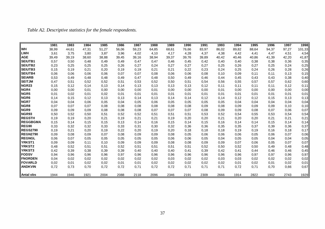
37

Table A2. Descriptive statistics for the female respondents.

1981 1983 1984 1985 1986 1987 1988 1989 1990 1991 1993 1994 1995 1996 1997 1998WH 38,99 44,61 47,31 51,27 56,06 59,23 64,85 68,61 76,66 83,97 86,02 89,82 88,64 94,37 97,27 101,33LWH 3,61 3,75 3,80 3,87 3,96 4,02 4,10 4,17 4,28 4,37 4,38 4,42 4,41 4,47 4,51 4,54AGE 39,49 39,19 38,60 38,88 39,45 39,16 38,94 39,37 39,76 39,89 40,42 40,46 40,86 41,39 42,20 41,87SEIUTB1 0,57 0,50 0,48 0,49 0,49 0,47 0,47 0,46 0,45 0,42 0,40 0,40 0,38 0,38 0,36 0,35SEIUTB2 0,23 0,25 0,25 0,25 0,26 0,27 0,24 0,27 0,27 0,27 0,25 0,26 0,27 0,25 0,24 0,25SEIUTB3 0,15 0,19 0,21 0,20 0,19 0,19 0,21 0,21 0,22 0,23 0,24 0,25 0,24 0,26 0,28 0,26SEIUTB4 0,06 0,06 0,06 0,06 0,07 0,07 0,08 0,06 0,06 0,08 0,10 0,09 0,11 0,11 0,13 0,15SEIARB 0,53 0,49 0,48 0,48 0,49 0,47 0,48 0,50 0,49 0,46 0,44 0,45 0,43 0,43 0,38 0,40SEITJM 0,47 0,51 0,52 0,52 0,51 0,53 0,52 0,50 0,51 0,54 0,56 0,55 0,57 0,57 0,62 0,60NGR23 0,15 0,12 0,14 0,13 0,14 0,13 0,13 0,13 0,13 0,12 0,11 0,11 0,11 0,11 0,12 0,11NGR4 0,00 0,00 0,01 0,00 0,00 0,00 0,01 0,00 0,00 0,00 0,01 0,00 0,00 0,00 0,00 0,00NGR5 0,01 0,02 0,01 0,02 0,01 0,01 0,01 0,01 0,01 0,01 0,01 0,01 0,01 0,01 0,01 0,01NGR6 0,14 0,15 0,12 0,13 0,13 0,14 0,13 0,14 0,14 0,12 0,14 0,12 0,12 0,15 0,13 0,13NGR7 0,04 0,04 0,06 0,05 0,04 0,05 0,06 0,05 0,05 0,05 0,05 0,04 0,04 0,04 0,04 0,04NGR8 0,07 0,07 0,07 0,08 0,08 0,08 0,08 0,08 0,08 0,09 0,08 0,09 0,09 0,09 0,10 0,10NGR9 0,09 0,09 0,09 0,08 0,08 0,08 0,07 0,07 0,07 0,08 0,09 0,09 0,08 0,07 0,06 0,07NGR93 0,50 0,52 0,50 0,51 0,52 0,52 0,51 0,51 0,51 0,53 0,52 0,54 0,55 0,53 0,54 0,54REGSTH 0,19 0,19 0,20 0,21 0,19 0,21 0,21 0,19 0,20 0,20 0,21 0,20 0,20 0,21 0,21 0,21REGGBGMA 0,15 0,14 0,15 0,15 0,13 0,14 0,16 0,15 0,14 0,15 0,16 0,14 0,14 0,15 0,14 0,14REG90 0,33 0,32 0,32 0,33 0,33 0,31 0,30 0,32 0,36 0,36 0,35 0,35 0,37 0,39 0,36 0,37REGS2790 0,19 0,21 0,20 0,19 0,22 0,20 0,19 0,20 0,18 0,18 0,18 0,19 0,19 0,16 0,18 0,17REGN2790 0,09 0,08 0,09 0,07 0,08 0,09 0,09 0,08 0,05 0,06 0,06 0,06 0,05 0,06 0,07 0,06REGNGL 0,06 0,07 0,05 0,05 0,05 0,05 0,05 0,06 0,06 0,05 0,04 0,05 0,05 0,04 0,04 0,05YRKST1 0,09 0,09 0,11 0,10 0,09 0,09 0,09 0,08 0,08 0,09 0,09 0,07 0,06 0,05 0,07 0,07YRKST2 0,48 0,52 0,51 0,51 0,52 0,51 0,51 0,51 0,51 0,52 0,50 0,52 0,50 0,49 0,48 0,48YRKST3 0,42 0,39 0,38 0,39 0,39 0,40 0,40 0,40 0,41 0,39 0,42 0,41 0,44 0,46 0,46 0,45FODSV 0,94 0,96 0,96 0,96 0,97 0,96 0,96 0,96 0,96 0,96 0,96 0,96 0,97 0,97 0,96 0,97FNORDEN 0,04 0,02 0,02 0,02 0,02 0,02 0,02 0,03 0,02 0,02 0,03 0,03 0,02 0,02 0,02 0,02FOVARLD 0,02 0,01 0,02 0,02 0,01 0,01 0,02 0,02 0,02 0,02 0,02 0,01 0,02 0,01 0,02 0,01ANDKVIN 0,72 0,73 0,70 0,72 0,72 0,71 0,72 0,72 0,71 0,71 0,71 0,72 0,71 0,70 0,66 0,67

Antal obs 1944 1946 1921 2004 2088 2118 2096 2346 2191 2309 2666 1914 2822 1902 2743 1929

38

Table A3. Descriptive statistics for the male respondents.

1981 1983 1984 1985 1986 1987 1988 1989 1990 1991 1993 1994 1995 1996 1997 1998WH 46,29 51,92 54,59 59,72 64,31 68,65 76,07 79,97 93,55 101,53 105,79 110,31 110,77 118,17 120,37 125,36LWH 3,78 3,88 3,94 4,03 4,10 4,17 4,27 4,33 4,47 4,55 4,58 4,62 4,63 4,68 4,71 4,75AGE 39,18 39,52 39,15 38,88 39,43 39,38 38,94 38,92 39,70 39,67 40,08 40,82 40,13 40,62 40,65 41,06SEIUTB1 0,31 0,30 0,31 0,32 0,33 0,31 0,30 0,31 0,28 0,29 0,26 0,27 0,28 0,28 0,27 0,25SEIUTB2 0,35 0,37 0,37 0,34 0,33 0,33 0,34 0,36 0,34 0,32 0,32 0,31 0,32 0,31 0,30 0,30SEIUTB3 0,22 0,20 0,19 0,21 0,21 0,21 0,22 0,22 0,22 0,26 0,26 0,25 0,25 0,25 0,26 0,26SEIUTB4 0,13 0,12 0,13 0,13 0,13 0,14 0,14 0,11 0,16 0,13 0,16 0,17 0,15 0,16 0,17 0,20SEIARB 0,52 0,55 0,57 0,53 0,54 0,53 0,53 0,57 0,52 0,50 0,48 0,49 0,49 0,47 0,47 0,45SEITJM 0,48 0,45 0,43 0,47 0,46 0,47 0,47 0,43 0,48 0,50 0,52 0,51 0,51 0,53 0,53 0,55NGR23 0,37 0,35 0,38 0,39 0,37 0,35 0,34 0,35 0,33 0,32 0,31 0,32 0,33 0,31 0,33 0,32NGR4 0,02 0,02 0,01 0,01 0,02 0,02 0,02 0,01 0,02 0,02 0,01 0,01 0,01 0,01 0,01 0,01NGR5 0,10 0,12 0,11 0,10 0,10 0,11 0,12 0,12 0,12 0,12 0,12 0,12 0,10 0,12 0,10 0,10NGR6 0,11 0,13 0,11 0,10 0,11 0,11 0,12 0,12 0,12 0,11 0,14 0,12 0,14 0,13 0,14 0,15NGR7 0,12 0,10 0,10 0,09 0,12 0,12 0,11 0,10 0,10 0,11 0,09 0,09 0,08 0,10 0,09 0,10NGR8 0,07 0,06 0,07 0,07 0,07 0,09 0,08 0,07 0,09 0,09 0,11 0,11 0,13 0,12 0,12 0,13NGR9 0,09 0,10 0,10 0,09 0,09 0,09 0,10 0,09 0,08 0,09 0,09 0,09 0,07 0,07 0,07 0,06NGR93 0,12 0,12 0,12 0,14 0,11 0,11 0,13 0,12 0,13 0,13 0,13 0,14 0,14 0,14 0,14 0,14REGSTH 0,19 0,18 0,19 0,19 0,17 0,18 0,18 0,18 0,19 0,19 0,21 0,19 0,21 0,20 0,16 0,19REGGBGM 0,16 0,14 0,15 0,14 0,17 0,16 0,16 0,16 0,15 0,15 0,14 0,14 0,15 0,14 0,14 0,15REG90 0,33 0,31 0,32 0,31 0,32 0,32 0,34 0,32 0,36 0,37 0,36 0,37 0,37 0,37 0,41 0,39REGS2790 0,20 0,22 0,22 0,22 0,21 0,20 0,20 0,21 0,19 0,18 0,19 0,19 0,18 0,20 0,19 0,17REGN2790 0,07 0,08 0,07 0,08 0,08 0,07 0,08 0,08 0,05 0,06 0,06 0,06 0,05 0,05 0,06 0,06REGNGL 0,05 0,07 0,05 0,06 0,06 0,05 0,05 0,05 0,05 0,05 0,04 0,05 0,04 0,04 0,05 0,05YRKST1 0,13 0,16 0,14 0,13 0,13 0,13 0,11 0,09 0,10 0,12 0,11 0,08 0,07 0,07 0,08 0,06YRKST2 0,13 0,13 0,15 0,17 0,15 0,14 0,15 0,14 0,14 0,14 0,12 0,14 0,12 0,13 0,12 0,11YRKST3 0,74 0,71 0,72 0,71 0,73 0,73 0,73 0,76 0,76 0,74 0,77 0,78 0,82 0,80 0,81 0,83FODSV 0,95 0,95 0,96 0,96 0,97 0,96 0,96 0,95 0,95 0,96 0,97 0,97 0,97 0,97 0,97 0,97FNORDEN 0,03 0,03 0,03 0,02 0,02 0,02 0,02 0,02 0,02 0,02 0,02 0,01 0,02 0,01 0,01 0,01FOVARLD 0,02 0,01 0,02 0,01 0,01 0,02 0,02 0,02 0,03 0,02 0,02 0,01 0,02 0,02 0,02 0,01ANDKVIN 0,28 0,27 0,27 0,29 0,27 0,29 0,28 0,28 0,29 0,29 0,30 0,31 0,31 0,30 0,29 0,29

Antal obs 1551 1588 1478 1491 1795 2159 2089 2598 2199 2246 2827 1816 2744 1892 2781 1912

39

Table A4. Regression results, women, some selected years.

1981 1986 1991 1995 1998

Variables Par. Est st-error Par. Est st-error Par. Est st-error Par. Est st-error Par. est st-errorINTERCEPT 3.300** 0.106 3.568** 0.105 4.290** 0.079 3.732** 0.098 3.993** 0.117

AGE 0.012* 0.005 0.015** 0.005 0.000 0.004 0.026** 0.005 0.021** 0.005

AGE2 * 1000 0.102 0.066 -0.153** 0.059 0.050 0.047 -0.229** 0.056 -0.160* 0.064

SEIUTB1 -0.081** 0.026 -0.024 0.020 -0.074** 0.017 -0.013 0.020 -0.084** 0.022

SEIUTB3 0.067 0.036 0.066** 0.024 0.117** 0.018 0.080** 0.021 0.082** 0.025

SEIUTB4 0.325** 0.049 0.222** 0.030 0.274** 0.030 0.275** 0.030 0.237** 0.032

SEITJM -0.021 0.025 -0.010 0.022 -0.039* 0.017 0.006 0.021 0.013 0.023

NGR4 0.028 0.081 -0.266 0.160 -0.029 0.087 0.101 0.072 -0.165 0.105

NGR5 0.017 0.105 -0.013 0.074 -0.021 0.040 -0.095 0.128 -0.146 0.114

NGR6 -0.052 0.037 -0.096** 0.036 -0.058* 0.025 0.016 0.036 -0.076* 0.034

NGR7 -0.008 0.070 0.059 0.036 0.000 0.039 0.007 0.047 -0.014 0.043

NGR8 -0.037 0.039 0.002 0.037 0.007 0.031 0.000 0.036 -0.039 0.040

NGR9 -0.086 0.049 -0.001 0.043 -0.078* 0.035 -0.012 0.041 -0.096 0.050

NGR93 -0.082 0.048 -0.052 0.038 -0.025 0.032 -0.063 0.036 -0.161** 0.041

REGSTH 0.011 0.029 0.019 0.025 0.078** 0.021 0.062* 0.025 0.092** 0.028

REGGBGMA -0.015 0.038 -0.013 0.028 0.026 0.022 0.074** 0.027 0.098** 0.028

REG90 -0.010 0.027 -0.005 0.022 0.022 0.017 0.019 0.023 0.011 0.023

REGN2790 -0.016 0.037 0.108** 0.039 0.005 0.027 0.006 0.035 0.030 0.035

REGNGL -0.008 0.038 0.006 0.040 0.029 0.028 -0.008 0.032 -0.036 0.040

YRKST1 0.068 0.041 -0.052 0.029 0.000 0.029 -0.033 0.041 -0.066 0.048

YRKST2 0.057 0.037 -0.007 0.031 -0.036 0.026 0.030 0.026 0.019 0.033

FNORDEN 0.109 0.063 0.067 0.058 -0.032 0.048 -0.064 0.049 -0.085 0.054

FOVARLD 0.025 0.058 0.041 0.062 -0.108* 0.048 -0.118* 0.053 -0.071 0.052

ANDKVIN 0.113* 0.051 0.100** 0.036 0.053 0.030 -0.006 0.044 0.000 0.041

N 1944 2088 2309 2822 1929Adj-R2 0.1161 0.07522 0.1272 0.1320 0.1772

** Significant at 1%-level. * Significant at 5%-level

40

Table A5. Regression results, men, some selected years.

1981 1986 1991 1995 1998

Variables Par. Est st-error Par. Est st-error Par. Est st-error Par. Est st-error Par. est st-errorINTERCEPT 3.237** 0.151 3.519** 0.097 3.914** 0.085 3.865** 0.111 4.050** 0.105

AGE 0.017* 0.007 0.021** 0.005 0.025** 0.004 0.030** 0.005 0.025** 0.005

AGE2 * 1000 -0.142 0.084 -0.201** 0.055 -0.251** 0.053 -0.296** 0.064 -0.226** 0.063

SEIUTB1 -0.046 0.024 -0.033 0.020 -0.068** 0.017 -0.028 0.019 -0.072** 0.021

SEIUTB3 0.064 0.033 0.064* 0.030 0.040 0.028 -0.011 0.028 -0.031 0.032

SEIUTB4 0.351* 0.040 0.314** 0.035 0.311** 0.032 0.253** 0.030 0.228** 0.034

SEITJM 0.113** 0.033 0.104** 0.028 0.082** 0.026 0.147** 0.027 0.138** 0.030

NGR4 0.080 0.066 0.025 0.052 0.058 0.034 0.061 0.037 0.086 0.052

NGR5 0.013 0.036 -0.041 0.026 0.022 0.022 -0.067* 0.027 -0.166** 0.029

NGR6 -0.004 0.028 -0.107** 0.029 -0.037 0.026 -0.051* 0.026 -0.104** 0.026

NGR7 -0.029 0.036 -0.018 0.027 -0.042 0.026 -0.119** 0.027 0.003 0.027

NGR8 0.127** 0.044 0.007 0.033 0.038 0.031 -0.050 0.027 0.024 0.032

NGR9 -0.050 0.041 -0.088** 0.027 -0.063* 0.029 -0.106** 0.034 -0.077 0.050

NGR93 -0.011 0.060 -0.060 0.042 -0.102** 0.031 -0.122** 0.036 -0.167** 0.046

REGSTH 0.089** 0.032 0.142** 0.024 0.088** 0.024 0.091** 0.024 0.125** 0.029

REGGBGMA 0.022 0.029 0.075** 0.023 0.038 0.023 0.064* 0.026 0.114** 0.028

REG90 0.049 0.027 0.064** 0.021 0.017 0.017 0.040 0.021 0.051* 0.021

REGN2790 0.019 0.043 0.078** 0.028 0.035 0.031 0.010 0.040 0.033 0.039

REGNGL -0.004 0.048 -0.014 0.030 -0.005 0.038 0.008 0.033 -0.012 0.039

YRKST1 0.057 0.038 0.019 0.024 0.036 0.022 0.035 0.035 0.057 0.041

YRKST2 0.014 0.054 0.003 0.032 0.030 0.027 -0.080** 0.031 0.000 0.043

FNORDEN 0.005 0.045 0.022 0.073 0.081 0.077 0.019 0.053 -0.118** 0.041

FOVARLD 0.059 0.044 -0.139** 0.042 -0.116 0.059 -0.071 0.080 -0.221** 0.076

ANDKVIN -0.075 0.044 -0.089* 0.037 -0.079* 0.034 -0.065 0.033 -0.112* 0.046

N 1551 1795 2246 2744 1912Adj-R2 0.3562 0.3167 0.2446 0.2384 0.2765

** Significant at 1%-level. * Significant at 5%-level