W LWD, S NMR€¦ · has higher sensitivity and uses less power. A side-looking NMR tool usually is...
74
In: Advances in Engineering Research ISBN: 978-1-53613-842-9 Editor: Victoria M. Petrova © 2018 Nova Science Publishers, Inc. Chapter 1 WIRELINE, LWD, AND SURFACE NMR INSTRUMENTS AND APPLICATIONS FOR PETROLEUM RESERVOIR FORMATION EVALUATION Songhua Chen * and Lilong Li Halliburton, Houston, Texas, US ABSTRACT Downhole Nuclear Magnetic Resonance (NMR) logging tools use inside-out sensor configurations that are significantly different from laboratory NMR instruments. The inside-out design resulted in grossly inhomogeneous static and radio-frequency (RF) magnetic fields in the sensitive volume of the logging tool. Consequently, the spin evolution in off-resonance condition becomes important. The first part of the chapter describes the unique challenges of the logging tool hardware, measurements, and the spin-dynamics modeling, as well as data processing. The second part of the chapter describes typical NMR pulse sequences that are used for logging measurements, NMR responses for fluids in rock pore systems, and the petrophysical interpretation models and methodologies for petroleum reservoir formation evaluation. * Corresponding Author Email: [email protected]. No part of this digital document may be reproduced, stored in a retrieval system or transmitted commercially in any form or by any means. The publisher has taken reasonable care in the preparation of this digital document, but makes no expressed or implied warranty of any kind and assumes no responsibility for any errors or omissions. No liability is assumed for incidental or consequential damages in connection with or arising out of information contained herein. This digital document is sold with the clear understanding that the publisher is not engaged in rendering legal, medical or any other professional services.
Transcript of W LWD, S NMR€¦ · has higher sensitivity and uses less power. A side-looking NMR tool usually is...
In: Advances in Engineering Research ISBN: 978-1-53613-842-9
Editor: Victoria M. Petrova © 2018 Nova Science Publishers, Inc.
Chapter 1
WIRELINE, LWD, AND SURFACE
NMR INSTRUMENTS AND APPLICATIONS
FOR PETROLEUM RESERVOIR
FORMATION EVALUATION
Songhua Chen* and Lilong Li Halliburton, Houston, Texas, US
ABSTRACT
Downhole Nuclear Magnetic Resonance (NMR) logging tools use
inside-out sensor configurations that are significantly different from
laboratory NMR instruments. The inside-out design resulted in grossly
inhomogeneous static and radio-frequency (RF) magnetic fields in the
sensitive volume of the logging tool. Consequently, the spin evolution in
off-resonance condition becomes important. The first part of the chapter
describes the unique challenges of the logging tool hardware,
measurements, and the spin-dynamics modeling, as well as data
processing. The second part of the chapter describes typical NMR pulse
sequences that are used for logging measurements, NMR responses for
fluids in rock pore systems, and the petrophysical interpretation models
and methodologies for petroleum reservoir formation evaluation.
* Corresponding Author Email: [email protected].
No part of this digital document may be reproduced, stored in a retrieval system or transmitted commercially in any form or by any means. The publisher has taken reasonable care in the preparation of this digital document, but makes no expressed or implied warranty of any kind and assumes no responsibility for any errors or omissions. No liability is assumed for incidental or consequential damages in connection with or arising out of information contained herein. This digital document is sold with the clear understanding that the publisher is not engaged in rendering legal, medical or any other professional services.

Songhua Chen and Lilong Li 2
INTRODUCTION
Understanding petroleum reservoir formation texture, pore size
distribution, pore connectivity, fluid saturation, and mobility is
overwhelmingly important for assessing the value of oil and gas reservoirs
and designing petroleum well completion and production operations.
Various sensor types have been developed for downhole well logging. The
measurement techniques used in well logging instruments are generally
from these broad categories: electrical (primarily resistivity and induction),
nuclear (primarily natural gamma, density, and neutron detection),
acoustic, optical, and nuclear magnetic resonance (NMR) (primarily proton
density, relaxation times, and diffusivity). Among those, electrical
measurements dominantly respond to fluid conductivity in reservoir
formation rock; optical techniques detect the fluid properties, such as fluid
types and compositions, while nuclear and acoustic techniques are more
sensitive to the rock matrix properties, such as mineralogy and lithology.
Compared to the non-NMR techniques, only proton NMR spin density
measurement directly measures the number of protons in the fluids in pore
space; thus, it is the only direct porosity measurement technique available
in downhole measurements. The relaxation and diffusion measurements
can be used for both rock texture assessment and fluid typing and
quantification, as well as to characterize fluid properties, such as viscosity
and gas-to-oil ratio (GOR). The versatility of NMR measurement
techniques enables various applications for formation evaluation, rock-
fluid interaction, multiphase fluid discrimination inside pore space, for
both in-situ downhole logging and laboratory rock, drill cutting, and fluid
characterization.
The physics of all NMR applications for petroleum reservoir rock and
fluid properties are based on (1) spin-density measurements for fluid in
pore space, which provides quantification of porosity and fluid content, (2)
molecular interactions of protons in pore fluid with minerals at the
surrounding pore wall, which is the origin for rock texture and wettability
estimation, (3) Stokes-Einstein equation governing the diffusivity and fluid
viscosity and either direct dipolar-dipolar interaction or spin-rotation

Wireline, LWD, and Surface NMR Instruments and Applications … 3
governing the bulk fluid relaxation time including both hydrocarbon
liquids and gases, as well as water.
NMR spectroscopy techniques are used for petroleum chemistry
applications to analyze molecular compositions of raw hydrocarbon fluids
and other related products. Real-time monitoring of the feed-forward and
feedback control in petroleum refinery is a niche application of NMR, such
as for detecting sulfur content, API gravity, viscosity, and Reid vapor
pressure (RVP) for volatility in raw petroleum feedstock or in refined
products. Edwards (2011) provides the most recent summary of the
petrochemical applications. Here, we do not intend to discuss such
downstream applications. Instead, we will focus on the upstream
applications related to the exploration of reservoir formation and fluid
using primarily low-field NMR instruments.
OVERVIEW OF CHALLENGES OF DOWNHOLE
NMR TOOLS
Wireline logging and logging while drilling (LWD) are two common
modes of openhole well logging operations. During wireline logging, one
or more logging tools are suspended by a coaxial cable and lowered into a
wellbore (e.g., borehole). The cable provides the mechanical strength and
the means for power and data transmission. Because the cable tension is
provided by the gravitational force on the sensors, wireline NMR logging
tools can only operate in vertical wells or low-angle deviated wellbores;
they cannot be used in horizontal wellbores. Petrophysical properties of the
rock formation and the fluid contained therein are measured and recorded
as a function of depth. During LWD, the logging tools are conveyed
downhole as part of the drilling assembly, and well logging is performed at
the same time as the drilling operation. LWD sensors are attached to the
drilling tool assembly; therefore, they can be operated in vertical,
horizontal, or any degree of deviated wells.

Songhua Chen and Lilong Li 4
In either mode, the logging tool resides in the borehole and faces
outside, into the formation. This “inside-out” constraint on NMR logging
stands in contrast to common laboratory NMR instrument configurations
where the sample is surrounded by magnets inside an NMR coil. This leads
to several consequences. First, the NMR coil placed far away from the
sensitive volume has low sensitivity. Thus, in NMR tool design, achieving
adequate signal-to-noise ratio (SNR) is always challenging. Another
consequence is that with the exception of early Earth’s field NMR logging
attempts, both the static (B0) and radio frequency (RF) magnetic field (B1)
are grossly inhomogeneous. Any chemical shift information is drowned by
the B0 field inhomogeneity. Therefore, normal NMR spectroscopic
techniques are inapplicable and only relaxation and diffusion
measurements are possible during NMR logging. A third consequence is
that the off-resonance effect becomes an integral part of the NMR spin
dynamics, which leads to, for example, the stimulated echo effect, an
enhanced diffusion sensitivity, and the mixing of T1 and T2 relaxation
during a Carr-Purcell-Meiboom-Gill (CPMG) sequence. The most
significant effects will be further discussed in this chapter.
Another feature of the logging operation is motion. Except on rare
occasions in which station measurements are performed to improve SNR
and gain a better understanding of the formation properties at these specific
locations, the NMR logging tool is constantly in motion. The
characteristics of the motion, however, are different for wireline logging
and LWD. During wireline logging, motion is minimal in the transversal
dimensions but is fast in the longitudinal direction. During LWD, the
longitudinal motion depends on the rate of penetration (ROP) of the
logging operation and is usually not as fast. Drilling, however, induces fast
rotation, vibration, and bouncing, often in the sub-audible to low-audible
frequency range, and all movements occur primarily in the transversal
plane except some longitudinal bouncing. The nature of such motion can
be regular or irregular because of the constant variation of drilling speed,
drilling mud flow dynamics, and/or hardness of the formation rock during
drilling operations. These different types of motion pose different sets of

Wireline, LWD, and Surface NMR Instruments and Applications … 5
challenges. For example, for wireline tools, the requirement of the
magnetic field uniformity along the longitudinal direction can be stringent.
In addition, care should be taken to design magnets situated away from the
main measurement window to maintain proper prepolarization at different
logging speeds. For LWD tools, resilience against lateral motion is
required. To that end, a stabilizer is usually employed to reduce lateral
motion, and a “fat” sensitive region should be part of the design
requirement so that the NMR signal is less sensitive to tool lateral motion.
Figure 1. Examples of two different sensor designs for LWD NMR logging tools.

Songhua Chen and Lilong Li 6
Figure 2. Examples of wireline NMR logging instruments. MRIL®-Prime™ is a
centralized tool. MRIL-XL and XMR™ are side-looking tools.
Because of the need to accommodate rotational drilling operations,
NMR LWD tools always work in a centric mode: the tool remains in the
center of the borehole, and the drilling mud occupies the space between the
tool and the formation (Figure 1). The wireline tool has a “choice:” it can
either work in a centric fashion (Figure 2, left) or in an eccentric (“side-
looking” or pad) fashion (Figure 2, middle and right). In the side-looking
design, the tool is pressed against the formation, and the antenna is usually

Wireline, LWD, and Surface NMR Instruments and Applications … 7
placed as close to the formation as possible to minimize power
requirements and maximize reception sensitivity. Both design types have
advantages and disadvantages. A centric NMR tool has better B1
uniformity across all azimuthal directions and can better match B1 and B0
across an entire sensitive region (e.g., B1 and B0 are perpendicular to each
other, and a similar rotation angle is maintained). A centric tool also has a
larger sensitive volume all around the borehole. However, a side-looking
NMR tool, because of the closeness of the sensor to the volume of interest,
has higher sensitivity and uses less power. A side-looking NMR tool
usually is less prone to borehole rugosity and reading sodium signals from
the borehole. Its operation is also less influenced by mud conductivity.
The property of the permanent magnet and core material employed in
the logging tool design varies with temperature. Consequently, the
sensitive region with respect to a certain frequency might shift during the
logging operation because the wellbore and formation temperature is a
function of depth. Such a shift might be small for a gradient tool but not so
for a saddle point tool (see next section). Thus, for a saddle point sensitive
volume design, the temperature variation can potentially cause significant
uncertainty in quantifying the porosity of the formation. Therefore, a
saddle point tool should be meticulously calibrated and temperature
carefully monitored during logging operations.
HISTORY OF NMR LOGGING
The history of NMR logging up to 2000 is well described in literature
(Jackson, 2001). Only a brief overview from the perspective of logging
tool design is presented here.
Early NMR logging attempts (1950s to 1980s) at Chevron and
Schlumberger focused on Earth’s field NMR logging. A strong magnetic
field is produced at an angle to the Earth’s field by a coil that passes direct
current (DC). After a few seconds (several times T1), the current is abruptly
switched off. The resulting polarization precesses around the Earth’s field
and generates a free induction decay (FID) signal, which is recorded. There

Songhua Chen and Lilong Li 8
are some inherent shortcomings with this type of design. First, the current
switch cannot be instantaneous and the ringdown can be on the order of
tens of milliseconds. Thus, NMR logging can only detect “effective
porosity” or “free fluid volume,” not the total porosity. Secondly, to kill
the borehole signal, the mud has to be doped with magnetic particles or
paramagnetic ions. This complicates the drilling process and adds to the
costs. Another shortcoming is mud containing paramagnetic ions can
invade the formation and kill or distort the signal in the formation, thus
creating uncertainties in porosity interpretation. If the mud contains
magnetic particles that cannot invade the formation, it might distort the
Earth’s field near the borehole and distort the porosity characterization as
well. Finally, the amplitude of the Earth’s field changes from location to
location, and the orientation with respect to the borehole might change as
well, which creates further complexities during data acquisition and
interpretation. Because of these and other shortcomings, the early Earth’s
field NMR logging technique was not commercially successful.
Jasper A. Jackson, of Los Alamos National Libraries, developed an
NMR logging sensor design in the early 1980s. Jackson realized that by
placing two opposing magnetic poles from two cylindrical magnets
together, a donut-shaped region surrounding the poles will have close to
zero magnetic field gradient (Jackson & Cooper, 1980) (Figure 3). Because
of the low magnetic field gradient, a sufficiently large sensitive volume
might produce an adequate NMR signal. This design represents the first
attempt to utilize permanent magnets and pulsed RF to perform NMR
logging. Obviously, the design concept was not incorporated into wireline
logging because longitudinally the sensitive volume is too short for fast
wireline motion. More than two decades later, Jackson’s design concept
was incorporated into LWD NMR logging with great success.
In the 1980s, NUMAR Corporation began optimizing the Jackson
design, but ultimately abandoned it in favor of a design that employs a
transversal static field dipole and a transversal RF dipole. In this design,
the sensitive volume is the shape of a thin cylindrical shell. Although the

Wireline, LWD, and Surface NMR Instruments and Applications … 9
shell is thin (on the order of 1 mm), it can be made significantly long to
dramatically increase the sensitive volume, thereby improving SNR. In
addition, multi-frequency acquisition becomes possible because the
frequency is no longer tied to a single saddle point. Because of other
available frequencies, time spent waiting for the recovery in one frequency
band is not wasted but used for data acquisition in other frequency bands.
Furthermore, such a design with high gradient enables the extraction of
diffusion information, which leads to significant advancements in NMR
fluid typing. The departure from the Jackson design was a bold move
because at the time it was hard to predict whether such a thin volume could
survive motion on the order of 1 second long and produce sustained CPMG
echoes.
Later in the 1990s, Schlumberger developed a design that can be
viewed as a modified Jackson design (MacInnis et al., 1995). Instead of
having two poles longitudinally opposed, they are placed on the same side
in the transversal plane, and the saddle point is formed in front of the two
poles. The magnet can be made much longer longitudinally to allow for
continuous logging, thus overcoming a significant issue in the Jackson
design. The operation mode of this design is also unique because the tool is
eccentric and pressed against the borehole on the antenna side. Because of
the proximity of the antenna to the sensitive volume and high frequency,
this design provides good SNR. However, because of the low gradient,
fluid typing becomes difficult. The saddle point design allows a single
frequency operation only.
From late 1990 to the early 2000s, Halliburton (who acquired Numar),
Baker Hughes, and Schlumberger all introduced commercial NMR
wireline logging products that employ transversal dipole for both the static
and RF field but work in the side-looking fashion. A side-looking NMR
tool generally uses less power, is less sensitive to mud and borehole
condition, can be used in a wider range of borehole sizes, and is easier to
position in the borehole. Later, Weatherford commercialized a centralized
single frequency NMR logging tool (NMRT™ sensor). With the exception

Songhua Chen and Lilong Li 10
of Weatherford, major NMR logging service providers all gravitated
toward multi-frequency side-looking designs for their wireline tools. Such
a design is particularly suitable for fluid typing because (1) the dynamic
range of the magnet field gradient, which determines how sensitive the tool
can be in characterizing diffusivity of the fluids, is far larger in a side-
looking multi-frequency design; (2) the time spent waiting for recovery in
one frequency can be utilized for data acquisition in another frequency,
particularly for formations containing signals with long relaxation times.
For the same reasons, these tools generally have longer antenna aperture,
allowing minimal variation of sensitive volume coverage for data acquired
in different frequencies.
On the LWD side, Halliburton pioneered LWD NMR logging in the
early 2000s with a design similar to the earlier NUMAR wireline design
using centralized transversal dipole magnets and transversal dipole
antenna. The thin sensitive volume in a rough drilling environment limits
the acquisition to T1 mode only because a long T2 CPMG train becomes
infeasible. Subsequently, other major LWD NMR service providers
designed LWD NMR instruments substantially similar to or a modification
of Jackson’s originally patented design.
Figure 3. Illustration of the Jackson magnet design [reproduced from (Jackson &
Cooper, 1980)]. Two opposing magnetic poles create a ring-shaped low-gradient
region (saddle point) around the magnets out in the formation.

Wireline, LWD, and Surface NMR Instruments and Applications … 11
SENSOR CONFIGURATIONS FOR DOWNHOLE LOGGING
Figure 4 illustrates some of the possible combinations of magnet and
antenna configurations. Magnet configurations (from left to right) can be
described as “longitudinal dipole,” “transversal dipole,” and “monopole”
and likewise for the antenna configurations (from top to bottom). Because
the static and RF magnetic fields need to be substantially perpendicular to
each other, some of the combinations are infeasible and therefore crossed
out.
Figure 4. Possible combinations of magnet and antenna configurations.

Songhua Chen and Lilong Li 12
Features of the magnet field can make a configuration more suitable
for a particular type of logging operation. For example, a transversal dipole
magnet can be made sufficiently long to offer practical translational
symmetry and thus is suitable for wireline logging where the logging tool
moves fast longitudinally but does not rotate. A longitudinal dipole or a
monopole magnet can be easily made rotationally symmetric and is
suitable for LWD where drilling causes fast rotation but the longitudinal
movement is slow.
The monopole magnet (i.e., Jackson design) has a ring-shaped area
around the magnet where the magnetic field gradient is near zero. This area
is called the saddle point and is usually the targeted area where the NMR
signal originates. A saddle point configuration is usually “fat” because of
the low gradient; therefore, the configuration is particularly robust against
the harsh rattling and vibrational motion during a drilling operation. On the
other hand, a transversal dipole magnet generally has a strong magnetic
field gradient in the targeted area and is designed as a multiple depths of
investigation (DOI) gradient-type tool. Exceptions to this general rule
exist. For example, combinable magnetic resonance (CMR) (Flaum, 2000)
can be categorized as a transversal dipole design but utilizes the cross-
sectional area instead of the longitudinal plane to place two separate
magnet pieces and form a saddle point in front of the tool.
The saddle point design targets a region near the zero magnetic field
gradient and thus covers a relatively large space and is less sensitive to
vibrational motion. However, complications can arise from the low
gradient because of the temperature dependence of the magnetization. As
the downhole temperature changes, the magnetic field strength varies
linearly with the temperature. If the RF remains the same, the sensitive
region distorts in shape and shift in depth. Consequently, an elaborate
scheme of calibration and possibly frequency control is required if porosity
values from the CPMG data are to be trusted. For a gradient design, such
concern is secondary because the sensitive region shift with respect to
temperature change is much smaller.

Wireline, LWD, and Surface NMR Instruments and Applications … 13
Of the three possible antenna configurations, the longitudinal dipole
and monopole magnets are more sensitive to mud conductivity because in
these two configurations the eddy current can easily circle around the tool
in the borehole. In a water-based mud (WBM) environment, particularly
when salt concentration is high, resistive loss during RF excitation can be
significant, which results in high power demand. High resistive loss also
corresponds to high noise, resulting in poor SNR. In contrast, the
transversal dipole antenna configuration is less sensitive to borehole mud
conductivity, particularly when the tool is designed to operate in a side-
looking mode where the antenna is positioned near the formation.
Longitudinal dipole configuration for the static field (Reiderman &
Chen, 2015; 2016), similar to the monopole configuration, can have
inherent rotational symmetry that makes it suitable for LWD operations.
Relative to the transversal dipole configuration, the magnetic poles are
farther away from the sensitive region; thus, the magnetic field gradient
can be lower. Through careful design (Jachmann et al., 2017), this
configuration can have a field gradient slightly larger than that of the
monopole configuration, with a much longer sensitive region. Combining
the longitudinal dipole magnet with the transversal dipole antenna, which
generally has greater sensitivity than the longitudinal dipole antenna,
particularly when the tool diameter is larger, is anticipated to further
improve the SNR of LWD NMR logging. Because of the concentric
operation of the LWD tool, two transversal dipole antennae can be placed
orthogonal to each other, without mutual interference. A circular polarized
NMR sensor can therefore be achieved in this design type. Circular
polarized excitation reduces the power consumption by a factor of 2, and
orthogonal reception increases the SNR by a factor of √2. One can take
advantage of the increased efficiency in excitation by reducing the pulse
width, therefore increasing the excitation bandwidth, which increases the
sensitive volume and further improves the robustness of the tool against
drilling motion. Another advantage of the transversal antenna is that the
eddy current cannot easily close in the borehole; therefore, this design
combination has even better SNR and power requirement attributes in a

Songhua Chen and Lilong Li 14
WBM environment. Conceivably, this design can incorporate multi-
frequency operation, which will improve SNR per unit time.
During NMR logging tool design, a figure of merit that is often
considered is SNR/√P (signal noise ratio over square root of power).
However, this figure of merit is more useful when SNR is power-limited.
Such is the case for a centralized tool with a long aperture. When sufficient
power can always be delivered, the tool becomes bandwidth-limited, and
the total SNR is a more important figure of merit. To convert the available
power to SNR, one can expand (1) in the transversal direction by utilizing
multiple frequencies; (2) in the longitudinal direction with a longer
antenna; (3) in the longitudinal direction using multiple antennae. The
antenna length should be balanced with the vertical resolution of the log.
Therefore, the appropriate course of action is to select the proper antenna
length and expand transversally to a larger DOI and lower frequencies to
achieve higher SNR. At some point, the SNR of the lower frequencies
becomes so poor that it does not add much to the total SNR. If sufficient
power remains available at this point, a longer antenna or an additional
antenna can be considered. For some antenna designs, a longer length will
make the antenna more efficient (B1 per unit current is larger) and thus is
preferred. For other antenna designs, a longer length will make the antenna
less efficient; thus, multiple short antennae are more preferred.
FINITE ELEMENT MODELING AND SPIN
DYNAMICS SIMULATION
Modern finite element (FE) modeling packages make accurate
modeling of the static and RF fields (B0 and B1) possible. Combining FE
modeling with spin dynamics simulation enables accurate prediction of the
behavior of the spin system and the echo signal generated in the receiver.
Actual pulse shape and the receiving circuit can also be part of the
simulation. Therefore, the integration of FE modeling and spin dynamics
simulation is essential to modern NMR logging tool design. The simulated
NMR echoes prove to be highly accurate (Figure 5). Using simulated NMR

Wireline, LWD, and Surface NMR Instruments and Applications … 15
echoes, we can study spin physics, the diffusion effect, and the motion
effect.
Stimulated Echo
For a CPMG echo train in a grossly inhomogeneous field, only the first
echo is a direct echo; from the second echo, the contribution of indirect or
stimulated echo becomes increasingly important (Goelman & Prammer,
1995). Despite the increasing contribution of indirect echoes, the echo
amplitude follows an exponential relaxation behavior, except for the first
few echoes (Goelman & Prammer, 1995; Hürlimann & Griffin, 2000).
Thus, the stimulated echo correction is only necessary for the first few
echoes. This stimulated echo correction, however, is closely related to the
exact distribution of the B0 and B1 fields, the actual shape and amplitude of
the RF pulses, the filtering effect of the receiving circuit, and the digital
filter applied. With these elements all included in a combined FE modeling
and spin dynamics simulation package, we can simulate the stimulated
echo effect accurately.
Figure 5. The shape of an echo in a CPMG echo train, experimental vs. simulation,
with real and imaginary components.

Songhua Chen and Lilong Li 16
Figure 6 shows simulation results of the stimulated echo correction
factors for the Halliburton XMR™ tool compared to the experimental
results. The experimental and simulation results agree remarkably well
over a range of frequency bands and B1 amplitudes. It is worth mentioning
that usually the second echo goes above the exponential fitting of the echo
train, and the correction factor is less than 1. Because of the specific
distribution of the B0 and B1 of this tool, the correction factor for the
second echo is larger than 1. The simulation correctly predicts this fact.
Diffusion
In a weakly inhomogeneous field, it is well known that the additional
attenuation caused by molecular diffusion to CPMG amplitude can be
written as a diffusion relaxation term with the relaxation constant T2d
described by
Figure 6. Stimulated echo correction factors from simulation and experiments at
different B1 amplitudes. Here, B1 is normalized so that B1 = 1corresponds to maximum
signal amplitude. The stimulated echo correction factors include the porosity deficit
factor when B1 is not optimum.

Wireline, LWD, and Surface NMR Instruments and Applications … 17
1
𝑇2𝑑=
𝐷(𝛾∗𝐺∗𝑇𝐸)2
12, (1)
where D is the diffusion coefficient, γ is the gyromagnetic ratio, G is the
static field gradient, and TE is the inter-echo spacing of the CPMG
sequence. If the field gradient is strong, the off-resonance effect becomes
dominant, and diffusion relaxation begins to deviate from such behavior.
Through spin dynamics simulation (Figure 7), we can observe the
following (Hürlimann, 2001):
The first few echoes have a different relaxation behavior, while in
the remaining echoes (from the fourth echo on), the diffusion
relaxation becomes the same and can be described as a function of
𝐷(𝛾∗𝐺∗𝑇𝐸)2𝑡
12.
Because of the difference in relaxation for the first few echoes, the
apparent stimulated echo correction changes as a function of
𝐷𝛾2𝐺2𝑇𝐸3, and the apparent porosity deviates from the actual
porosity as a function of 𝐷𝛾2𝐺2𝑇𝐸3 as well. During NMR data
interpretation, because the diffusivity is unknown, it is best to
account for such deviations in the data inversion process.
Amplitude of Partially Recovered CPMG
During NMR logging, the SNR calculation is always challenging
compared to laboratory conditions. Additionally, logging operations need
to be performed as quickly as possible. As a result, for shorter wait times
(TWs) that do not reach full polarization of the spins, the CPMG train is
often performed after whatever the spin state the system is left with before
the wait time, and it inevitably introduces some error. A saturation pulse(s)
might not help much in such case when both B0 and B1 fields are grossly
inhomogeneous.

Songhua Chen and Lilong Li 18
Figure 7. The effect of diffusion on stimulated echo correction. Blue curve: data from
simulation; green curve: exponential fit of simulated data from the fourth to 20th
echo. Except for diffusion-caused relaxation, T1 and T2 are assumed to be infinite
in simulation.
An example of such partially recovered sequence is a trainlet sequence
wherein short CPMG echo trains with a limited number of echoes (NE) and
usually short TWs are applied repeatedly (Sezginer & Straley, 1995; Chen
& Edwards, 2002). This trainlet sequence is performed frequently during
NMR logging operations. If the trainlets are applied in exactly the same
manner, they will suffer steady-state buildup that will gravely distort the
signal amplitude (Freed et al., 2001). To minimize this steady-state
buildup, immediate phase alternated pairs (PAPs) are commonly used
(Sezginer & Straley, 1995). Such immediate PAPs cannot completely
remove extra amplitude buildup. In the absence of diffusion, it is even
more obvious (Figure 8). Figure 8 illustrates that without diffusion, the
amplitude settles at approximately 0.15 instead of the theoretical 0.1—an
error of more than 50%. With a longer TW, spins have more time to relax,
and the relative error is smaller. To reduce the overall relative error, one
can interleave different TWs. Figure 9 illustrates the advantage of
interleaving, wherein the actual amplitude of the partially recovered

Wireline, LWD, and Surface NMR Instruments and Applications … 19
Figure 8. Spin dynamics simulation of trainlets. Simulation parameters are as follows:
T1 = T2 = 100 ms, TE = 0.3 ms; NE = 20; TW = 10.5 ms. Spins are saturated before
application of the trainlet sequence. The amplitude of a fully polarized spin echo train
is normalized to 1. The sharp abnormality at the end of the trainlets is caused by
previous excitations with the same NE and will diminish with the presence of
diffusion.
Figure 9. Trainlets with different TWs before repeating. Parameters used here are the
same except the TWs are 10.5, 22.3, and 35.7 ms. The corresponding echo amplitudes
should be 0.1, 0.2, and 0.3, assuming the amplitude of the fully polarized echo train
is 1.

Songhua Chen and Lilong Li 20
trainlets follows the theoretical values more closely. In the presence of
diffusion and static field gradient, the error observed in Figure 8 is reduced
but will not be eliminated with a combination of water diffusivity and a
field gradient of 0 to 40 G/cm in a logging tool. The interleaving scheme
becomes even more effective when diffusion and static field gradient are
both present.
Figure 10. Top: simulated echo trains; bottom: the echo train amplitude (blue)
compared to theoretical values (green). T1 and T2 of 100 ms are used. TWs are 230.3,
120.4, 69.3, 35.7, and 10.5 ms, respectively. NEs are 200, 50, 50, 20, 20, respectively.
TE is 0.3 ms for all echo trains.

Wireline, LWD, and Surface NMR Instruments and Applications … 21
TW interleaving works not only in trainlet sequences but also in T1
sequences in which different TWs are required to obtain the T1 recovery
curve. Figure 10 shows a particular scheme of acquisition where
immediate PAPs are acquired and TW decreases in descending order. In
this sequence, no additional waiting or saturation pulses are necessary. The
simulation is performed without diffusion effects. With diffusion effects,
the simulated amplitude is even closer to the theoretical values because of
the additional dephasing.
Such interleaving can be used in unexpected ways. After a long CPMG
echo train, because of steady-state buildup or incomplete dephasing, the
remaining spin order can distort the following CPMG echo trains if the TW
is not sufficiently long and spins are not completely recovered. It is also
difficult to completely saturate the spins with pulses when a wide
distribution of B0 and B1 as well as T1 and T2 are present. However, two
PAP short trainlets can be used as “sacrificial” trainlets, preferably with
smaller TE and NE, and achieve far smaller amplitude error for subsequent
partially recovered echo trains.
Longitudinal Motion
The artifacts resulting from longitudinal motion, if not meticulously
prevented, can originate from unexpected sources, one of which is the
longitudinal field gradient and the offset frequency shift during
longitudinal motion.
To understand this motional effect, we begin with the frequency
components of a CPMG echo. Figure 11 shows the Fourier transform of
the echo shape or the amplitude contribution from spins at different
frequency offsets (only half of the offset frequencies are plotted). During
the spin dynamics simulation that generated the result, we used Hanning
shaped pulses of 28 and 56 µs as excitation and refocusing pulses. TE is
0.5 ms.
We observe that the amplitude contribution from different offset
frequencies is not a smooth curve. Rather, it has fine structures and a

Songhua Chen and Lilong Li 22
periodicity of 1/TE (in this case 200 Hz). Now imagine a spin moves
slowly from one offset frequency to the other while a CPMG pulse
sequence is applied. The amplitude contribution from that spin will
fluctuate with a periodicity of 1/TE. Similarly, when a tool moves
longitudinally with a longitudinal B0 field gradient present, all of the spins
in different offset frequencies experience a shift in offset frequency during
a CPMG pulse sequence. If the fluctuations do not cancel each other, an
overall oscillation in echo amplitudes will occur, which is exactly what
occurs using spin dynamics simulation of an ideal case where B1 is
constant, and B0 has a singular gradient in the longitudinal direction
(Figure 12).
Figure 11. Signal amplitude as a function of frequency offset in a grossly
inhomogeneous field. The 180 pulse bandwidth is 35.7 kHz. TE = 0.5 ms. The bottom
plot is a zoom-in view of the top plot.

Wireline, LWD, and Surface NMR Instruments and Applications … 23
Figure 12. Amplitude oscillation of CPMG echoes in an ideal case where B1 is
constant, and B0 has a constant gradient of 0.0656 G/cm. Longitudinal speed is 10
ft/min (0.0508 m/s), and TE is 2 ms. The noise spike at approximately 0.7 s is a
numerical artifact when isochromats (spins at a particular frequency offset) are equally
spaced and all have the same gradient. The artifact does not influence the accuracy of
the overall simulation.
Figure 13. Amplitude decay of CPMG echoes in an ideal case where B1 is constant,
and B0 has a random gradient in the range of [-0.1312, 0.1312] G/cm. Longitudinal
speed is 10 ft/min (0.0508 m/s), and TE is 2 ms.

Songhua Chen and Lilong Li 24
In the actual tool, the longitudinal field gradients might not be all the
same but have a distribution—positive in some parts and negative in other
parts. Figure 13 shows a simulated case in which the B0 longitudinal
gradient is random with a uniform distribution in the range of [-0.1312,
0.1312] G/cm. The actual gradient controls the oscillation frequency in
Figure 12. The summation of different oscillations results in a sharp decay
at the beginning of the echo train. If the longitudinal gradient is sufficiently
large, the decay will be fast and might cause errors in the NMR logging
interpretation. Thus, care should be taken to ensure that the longitudinal
gradient falls within strict requirements. If the requirement cannot be met,
the actual field variation can be measured and simulation used to correct
for the actual signal amplitude at different logging speeds. The correction
should be perfomed on a tool-by-tool basis and therefore is not ideal.
Apart from the initial decline shown in Figure 13, the amplitude also
slowly decays because the region excited by the first 90° pulse gradually
moves out of the sensitive window of the antenna. In addition to causing
faster echo decay, longitudinal motion can also cause the initial amplitude
to deviate during a T1 recovery experiment (Jachmann et al., 2013). This is
because after the saturation pulse, and a certain wait time, the tool has
already moved to a new location where a portion of the spins did not
experience full saturation. The subsequent CPMG sequence will then
record an incorrect porosity. This effect, however, can be mitigated with
simulation and correct inversion (Jachmann et al., 2013).
LOW-FIELD NMR FLUID, CORE, AND MUD
LOGGING MEASUREMENTS
NMR fluid, core, and drill cutting analyzers are primarily surface
NMR instruments except for Halliburton’s MRILab® service, which is an
inline fluid NMR measurement device integrated in a downhole fluid
sampling tool. Because of its unique application, in this section, we first
discuss MRILab; the remainder of the section focuses on surface NMR
measurements.

Wireline, LWD, and Surface NMR Instruments and Applications … 25
Figure 14. MRILab® module on an RDT™ reservoir description tool for inline
fluid analysis.
Figure 14 shows an illustration of an MRILab tool section as an add-on
device to a Halliburton RDT™ reservoir description tool. The device
includes a long and strong magnetic field section for rapid proton
polarization before the RF coil section to allow adequate polarization of
protons in the inflow fluid. The inflow fluid is directly extracted from the
formation of reservoir depth. The RF transmitter coil is longer than the

Songhua Chen and Lilong Li 26
receiver coil in the RF coil section. The idea is that by exciting a larger
volume but receiving the NMR signal only from the bottom of the large
excitation volume, the relaxation time measurements are independent of
the incoming fluid flow rate (Prammer et al., 2007).
Figure 15. The ECOTEK Corporation automatic sample-loading system attached to a
low-field NMR apparatus (Courtesy of Arcady Reiderman, president of ECOTEK).
MRILab service is primarily used to obtain quantitative information
about mud filtrate contamination during the pump-out phase, before the
high-quality fluid samples are collected for pressure/volume/temperature
(PVT) analysis (Akkurt et al., 2004). This is particularly useful for
estimating contamination of oil-based mud filtrate (OBMF). During the
drilling process, OBMF invades the pore space in the near-wellbore region.
OBMF and the native reservoir oil are generally miscible macroscopically;
however, at the molecular level, the difference in intermolecular and
intramolecular dipole-dipole interaction appears maintaining bimodal T1
Wireline, LWD, and Surface NMR Instruments and Applications … 27
distribution between the OBMF and native oil T1 responses (Akkurt et al.,
2004). By observing the relative amplitude of the two peaks, or the overall
T1GM shift, the amount of OBMF that remains in the extracting samples can
be estimated. Such real-time mud-filtrate estimation is economically
important because the time necessary to collect samples downhole
translates to high rig time costs, and the quality of the samples is essential
to evaluate the reservoirs.
Mud logging usually involves large quantities of samples and requires
rapid throughput because the information is usually used while drilling.
Although traditional NMR desktop systems can be used to analyze drill
cuttings, they cannot provide fast-turnaround, low-cost measurements if
each sample needs to be prepared, loaded, system tuned, measured, and
unloaded one at a time. The labor costs make such operations prohibitive.
More recently, ECOTEK Corporation manufactured an automatic sample-
loading system attached to a low-field NMR instrument (Figure 15) as a
node of its advanced mud logging system. All sample sizes, system-tuning
procedures, and NMR pulse sequences are standardized and automatized.
This system minimizes the need for human interactions to run multiple
samples, making it particularly useful for high throughput of drill cutting
sample analysis at the wellsite or in the laboratory. It is also suitable for
core NMR measurements.
Most of the NMR fluid, core, and cutting analyses are conducted in a
surface laboratory or at the wellsite, primarily in an ambient environment.
Low-field NMR instruments are normally used for two reasons. First, the
majority of the interest in NMR core analysis is to provide calibration to
the NMR logging responses or develop petrophysical interpretation
models. Therefore, it is desirable to conduct laboratory NMR
measurements at a field strength close to that used in logging tools to
minimize any potential discrepancies. Secondly, most low-field NMR
devices are made with permanent magnets; thus, the cost of the instruments
and long-term maintenance are minimal. Because core NMR
measurements are similar to logging, we will not particularly separate core
measurements from logging in the remainder of this chapter.

Songhua Chen and Lilong Li 28
NMR LOGGING DATA ACQUISITION AND PROCESSING
One-Dimensional T1 and T2 Measurements
The most basic wireline NMR logging involves the T2 total porosity
sequence aiming to deliver total porosity and T2 distribution. This sequence
involves a fully polarized CPMG sequence with a sufficiently long echo
train (FP) capable of detecting the longest relaxation time components plus
one or more partially polarized short trainlets (PPTs) described in the
“Amplitude of Partially Recovered CPMG” section that emphasizes
obtaining high-SNR fast-decay components. Such combination of
1FP+nPPTs can also be duplicated with multi-frequency operations.
Figure 16 illustrates a data acquisition sequence with four frequencies.
Figure 16. A typical pulse sequence implemented in NMR logging for T2 total porosity
data acquisition.
The FP echo trains are normally acquired with 500 ms - 1 s of data; a
typical TW1 PPT acquires 6 ms of data, and a typical TW2 PPT acquires
20 ms of data, respectively. The number of echoes, number of repeats, and
the number echoes in a burst is typically designed to follow
[𝑛𝑒𝑐ℎ𝑜𝑒𝑠 × 𝑇𝐸 + 𝑇𝑊] × 𝑛𝑟𝑒𝑝𝑒𝑎𝑡 ≈ 𝑐𝑜𝑛𝑠𝑡. (2)
across all frequencies so that the FP echo train corresponding to each
frequency has substantially the same TW.

Wireline, LWD, and Surface NMR Instruments and Applications … 29
The TW corresponding to FP requires the protons be fully polarized
before FP echoes are acquired. A short antenna, single-frequency NMR
logging tool typically operates in a so-called non-overlapping mode,
meaning the TW only needs to be sufficiently long to satisfy
𝑇𝑊𝑚𝑖𝑛 = antenna aperture logging speed + 𝛿𝑡⁄ , (3)
assuming the tool has an adequately long pre-polarization magnet. In the
equation, 𝛿𝑡 is the time required for residual saturation from the previous
FP or PPTs to be re-polarized. If the formation and environment requires
substantial signal averaging, the non-overlapping model could potentially
result in poor vertical resolution.
For a multi-frequency operation, the number of frequencies, 𝑛𝑓𝑟𝑒𝑞, is
selected such that the TW for FP is sufficiently long to ensure the fastest
relaxing component of the fluids in the formation are fully polarized, or the
antenna aperture during TW has already moved out of the overlapping
window of the previous operation, whichever occurs first. Beyond that,
adding more frequencies does not achieve additional benefits from multi-
frequency operations. Multi-frequency operation is most suitable for low-
porosity reservoirs and high-salinity wells that require substantial signal
averaging.
The T2 of formation fluids usually varies between sub-milliseconds to a
few seconds. To recover the fast-decay components, the shortest possible
TE in the PPTs part of the pulse sequence is required. This requires high-
pulse RF power, which potentially causes significant acoustic ringing. To
eliminate the ringing induced by the refocusing (π) pulses, PAP data
acquisition is always used. However, the PAP method cannot reduce the
ringing of the excitation (π⁄2) pulse. To cancel the excitation pulse ringing,
a frequency dithering method (Beard, 2007) where the number of
frequency (𝑁𝑓) and the frequency difference (∆𝑓) satisfies
𝑁𝑓 ∙ ∆𝑓 = 𝑚 𝑇𝐸⁄ (4)
Songhua Chen and Lilong Li 30
where 𝑚 is an integer that can be chosen as 1. Note ∆𝑓 in the equation is
usually in the order of 1 kHz. For instance, 𝑁𝑓 = 4 and 𝑇𝐸 = 0.2 𝑚𝑠,
∆𝑓 = 1.25𝑘𝐻𝑧, which is within the bandwidth of the RF circuit and is
significantly different from the multi-frequency mode illustrated in Figure
16.
Although several LWD instruments also prefer to use single-frequency
T2 total-porosity logging mode, T1 total-porosity logging is the preferred
logging mode for a type of LWD NMR tool that operates in a gradient
field. Because the thickness of the sensitive volume of an NMR logging
instrument is proportional to the gradient strength,
∆𝑟 ∝1
𝐺∙𝑇𝐸, (5)
a high-gradient logging tool has a narrower sensitive volume thickness
than a low-gradient tool. LWD operates in a highly vibrational
environment; therefore, T2 logging that acquires substantially longer echo
trains would require that the majority of protons remain in the same
sensitive volume of the excitation pulse as that in the subsequent all-
refocusing pulses—an assumption that is too difficult to be practical for a
gradient LWD NMR tool. However, by applying a broadband chirp pulse
for the saturation pulse in a saturation recovery T1 logging mode and
narrow band short trainlets of excitation-refocusing pulses, the motion
problem during LWD NMR data acquisition can be bypassed. Figure 17
illustrates the difference.
Figure 17 (left) shows the LWD T1 mode. The yellow ring represents
the sensitive volume of the broadband chirp pulse, and the purple ring
represents the sensitive volume by the short excitation-refocusing trainlets.
Because the trainlets only take a few milliseconds to acquire; within
this time window, no significant lateral motion is expected to cumulate
because the drilling-induced motion has a frequency in the order of hertz.

Wireline, LWD, and Surface NMR Instruments and Applications … 31
Figure 17. Illustration of the motion sensitivity of T1 and T2 logging experiments. Left:
the yellow ring represents a wide sensitive volume (sv) defined by a broadband chirp
pulse acting as a saturation pulse. The purple ring represents the sensitive volume
defined by the recovery pulses of the saturation recovery pulse sequence for T1
measurement. Right: all excitation and refocusing pulses are narrow band pulses, thus
T2 is more sensitive to lateral motion while drilling.
In contrast, T2 logging mode usually acquires 500 ms of data, within which
the cumulative vibrational motion effect could be significant for a gradient
tool. Therefore, T2 logging is usually only preferred to a low-gradient tool,
which has a wider sensitive volume (Figure 17, right).
Two-Dimensional and Three-Dimensional NMR Measurements
Two-dimensional (2D) and three-dimensional (3D) NMR
measurements usually are used for fluid typing in conventional and
unconventional reservoirs. The most commonly used 2D sequences include
T1 − T2 sequence and T2 − D sequence, which involves many echo trains
with different TW, different TE, or a combination of both. In general, a 3D
sequence is simply a comprehensive sequence with more TE or TW
involved. We can symbolically write each echo train or PPT in a 3D
sequence as
𝐸𝑘(𝑓𝑘, 𝐺𝑘 ∙ 𝑇𝐸𝑘 , 𝑇𝑊𝑘 , 𝑁𝐸𝑘 , 𝑁𝑟𝑒𝑝𝑒𝑎𝑡,𝑘). (6)

Songhua Chen and Lilong Li 32
Two other approaches to generate NMR logging data suitable for 2D
or 3D NMR have also been reported. One approach is often referred to as
diffusion-editing sequence (Hürlimann et al., 2002) (Figure 18) in which
the first few echoes (usually two echoes) are acquired at a long TE (TEL),
followed by refocusing the remaining echoes at a substantially short TE
(TES). The TEL echoes obtain the most decay information because of
diffusion in a gradient field, while the TES echoes decay much slower
because the G∙TES factor is much smaller. It is possible to use different TEL
values for multiple diffusion-editing sequence elements or combining a
diffusion-editing sequence with traditional multi-TE, multi-TW sequences
described in Eq. (6).
Figure 18. Diffusion-editing sequence illustration (Hürlimann et al., 2002).
Figure 19. Illustration of an echo-decay-acceleration pulse sequence.
The second variation to Eq. (6) also uses two TE values. However, the
order of long and short TEs is simply reversed from the diffusion-editing
sequence. Figure 19 illustrates a version of such sequence where ns number
of echoes with short TES is acquired first, followed by the acquisition of nL

Wireline, LWD, and Surface NMR Instruments and Applications … 33
number of echoes with long TEL. The echo decay is accelerated for the TEL
echoes compared to the decay rate when a shorter TES is used. For this
reason, it is referred to as the echo-decay-acceleration sequence (Chen,
2010). The echo-decay-acceleration sequence is proposed for a reservoir
having fast relaxation components and is required for diffusion-based fluid
discrimination. The short TES echoes have high data density to recover all
porosity components accurately, while the TEL echoes are sensitive to the
decay of diffusion in the gradient associated with relatively slow relaxation
time components. If multiples of such sequences with different TEL are
used, the combination can yield similar sensitivity to multiple TEs for
diffusion-based fluid typing while improving the total porosity
determination.
A practical advantage of using the echo-decay-acceleration sequence
exists in multi-frequency operation mode. To process multi-frequency data
together, it is important to verify that individual frequencies are calibrated
and acquired consistently. With the same TES, echoes are acquired first in
the echo-decay-acceleration sequence for all frequencies and provide a
check point to compare porosity values from each frequency’s data. This is
not possible if either conventional CPMG sequence with different TEs or
the diffusion-editing approach is used for multi-frequency operations.
INVERSION
Petrophysical and reservoir characterization parameters are more
straightforwardly related to the T1-T2-D parameter than the time-domain
echo train data. Thus, inversion processing is usually applied to the NMR
logging measurements to transform the time-domain data to the parameter
domain information. Many inversion methods have been discussed in
literature. The inversion methods described in this section represent some
of the approaches currently used for commercial NMR logging operations.

Songhua Chen and Lilong Li 34
T2 Only Inversion
T2 Inversion Using Only One Fully Polarized Echo Train
The input echo trains are the time-based) data. When a single FP echo
train is acquired, the ith echo in the echo train is represented by
𝐸𝐹𝑃(𝑖, 𝑡𝐸𝐹𝑅) = ∑ 𝐸0,𝑚𝑀𝑚=1 exp (−
𝑖∗𝑡𝐸𝐹𝑃
𝑇2,𝑚). (7)
In matrix form, E=Ax, where A is the inversion matrix with element of
exp (−𝑖∗𝑡𝐸𝐹𝑃
𝑇2,𝑚) and x is the solution vector in the form of
𝑥 = [𝐸01
⋮𝐸0𝑀
]. (8)
The solution is obtained by the minimization
𝑚𝑖𝑛[(𝐴𝑥 − 𝑏)2 + 𝛼‖𝑊 ∙ 𝑥‖2],with 𝑥 ≥ 0, (9)
where W is the regularization matrix and α is the regularization parameter.
The solution of the Eq. (9) minimization without non-negative
constraints is
𝑥 = (𝐴′ ∗ 𝐴 + 𝛼𝑊′ ∗ 𝑊)−1𝐴′ ∗ 𝑏. (10)
T2 Inversion Involving FP and Multiple PPTs
A method is developed to correct the polarization effect on the PPTs
echoes. First, the n number of repeats in each of the PPTs echo trains are
stacked to obtain an averaged PPT, which is subsequently processed using
the T2 inversion method described in the previous section. The shortest T2
components from the T2 inversion can be considered fully polarized. For
example, components with a short T2 of less than 3 ms can be treated as
fully polarized for the PPTs echo trains with TW of only 10 ms. These

Wireline, LWD, and Surface NMR Instruments and Applications … 35
shortest T2 components are forward modeled to create fully polarized echo
trains and noted as polarization-corrected echo trains. The polarization-
corrected echo trains are processed with the acquired FP echo trains using
the T2 inversion described in the previous section. The matrix A can be
described as the following:
𝐴 =
[
𝑒−𝑇𝐸 𝑇21⁄ 𝑒−𝑇𝐸 𝑇22⁄ ⋯ 𝑒−𝑇𝐸 𝑇2𝜇⁄ 0 ⋯ ⋯ ⋯ 0⋮ ⋮ ⋮ ⋮ ⋮ ⋯ ⋮ ⋮ ⋮
𝑒−𝑁1𝑇𝐸 𝑇21⁄ 𝑒−𝑁1𝑡𝐸 𝑇22⁄ ⋯ 𝑒−𝑁1𝑇𝐸 𝑇2𝜇⁄ 0 ⋯ ⋯ ⋯ 0𝑒−𝑇𝐸 𝑇21⁄ 𝑒−𝑇𝐸 𝑇22⁄ ⋯ ⋯ ⋯ 𝑒−𝑇𝐸 𝑇2𝜐⁄ 0 ⋯ 0
⋮ ⋮ ⋮ ⋮ ⋮ ⋮ ⋮ ⋮ ⋮𝑒−𝑁2𝑇𝐸 𝑇21⁄ 𝑒−𝑁2𝑇𝐸 𝑇22⁄ ⋯ ⋯ ⋯ 𝑒−𝑁2𝑇𝐸 𝑇2𝜐⁄ 0 ⋯ 0𝑒−𝑇𝐸 𝑇21⁄ 𝑒−𝑇𝐸 𝑇22⁄ ⋯ ⋯ ⋯ ⋯ ⋯ ⋯ 𝑒−𝑇𝐸 𝑇2𝑀⁄
⋮ ⋮ ⋮ ⋮ ⋮ ⋮ ⋮ ⋮ ⋮𝑒−𝑁𝑇𝐸 𝑇21⁄ 𝑒−𝑁𝑇𝐸 𝑇22⁄ ⋯ ⋯ ⋯ ⋯ ⋯ ⋯ 𝑒−𝑁𝑇𝐸 𝑇2𝑀⁄ ]
(11)
Multi-Dimensional NMR Inversion
In the most general form of 3D inversion of multiple echo trains, an
individual echo in any of these multiple echo trains is described by
𝐸(𝑖, 𝑗, 𝑘, 𝑙) = ∑ ∑ ∑ 𝐸0,𝑚𝑛𝑝[1 − exp(− 𝑇𝑊𝑘 𝑇1,𝑚⁄ )]𝑃𝑝=1
𝑁𝑛=1
𝑀𝑚=1
exp(− 𝑖 ∙ 𝑇𝐸𝑗 𝑇2,𝑛⁄ ) exp(−𝛾2𝐺𝑙2 𝑖 ∙ 𝑇𝐸𝑗
3𝐷𝑝 12⁄ ) + noise, (12)
where E(i,j,k,l) is the ith echo in an echo train acquired with the jth inter-
echo time TEj and the kth wait time TWk, and the echo signals are
contributed from the lth sensitive volume in which the field gradient
strength the spins experience is Gl.
The solution E0,mnp is obtained by solving the linear equation sets in the
form of Eq. (12). Similar to the 1D inversion described in the previous
section, a non-negative constraint of
𝐸0,𝑚𝑛𝑝 ≥ 0 (13)
is imposed.

Songhua Chen and Lilong Li 36
Eq. (12) with Constraint Eq. (13) can be summarized as the following
linear system with non-negative constraint AX = b, X ≥ 0, where A is a
matrix with the size of L × M × N × P, and L is the number of echoes
and the number of rows of the matrix A. The number of unknowns is M ×
N × P.
For logging data involving a large number of echo trains, the size of M
× N × P can exceed the number of acquired echoes, resulting in an
underdetermined inversion problem. For example, the 3D NMR inversion
with the size of 30 × 30 × 30 has 27,000 unknowns, which exceed the
number of data acquired by any current NMR logging tools per data
acquisition cycle. Furthermore, the linear system described by Eq. (12) is
often solved by the least squares method. It involves the matrix
multiplication A’ × A and its inverse. The computation complexity of
matrix multiplication and inverse is O(M × N × P). For a 3D inversion with
a size of 20T2 × 20D × 20T1, the spectral resolution of T2 and T1 might be
insufficient for interpretation. Assuming the total number of acquired
echoes is 4,000, the matrix multiplication A’ × A in the MATLAB®
platform will take nearly 16 seconds even with the limited spectral
resolution; therefore, 3D NMR inversion is usually too time-consuming to
be used for field data interpretation. To overcome such cumbersome
numerical issues, often some simplification and reduction of dimensions
with valid physical constraints are used. A commonly used two-and-a-half-
dimensional (2.5D) inversion, described in the following section, becomes
a practical solution.
2.5D Inversion for D − T2 and D − T1 Map
In 2.5D inversion, a useful physical constraint is applied based on the
intrinsic T2 and T1 relationship of fluids in porous media. In general, the
ratio of bulk T1 to intrinsic bulk T2 of liquid-phase water, light or medium
viscous oils, and hydrocarbon gases are substantially close to unity. When
affected by pore surface, the ratio R = T1/T2int can increase somewhat, but

Wireline, LWD, and Surface NMR Instruments and Applications … 37
in general, is confined in the range of 1 to 5. Heavy oil and tar, however, is
also expected to have a higher T1/T2int ratio, but for the viscosity range
generally observable by the NMR logging instruments, the upper limit of
the ratio value is also limited to a single digit. A more generous constraint
1 ≤ (𝑅 ≡ 𝑇1 𝑇2⁄ ) ≤ 10 (14)
covers all conceivable ranges of R. In the inversion when this constraint is
applied, R is discretized with only two or three grid points. With the
constraint of Eq. (14), the 3D inversion problem matrix size is significantly
reduced to what often is called the 2.5D inversion
𝐸(𝑖, 𝑗, 𝑘, 𝑙) = ∑ ∑ ∑ 𝐸0,𝑚𝑛𝑝[1 − exp(− 𝑇𝑊𝑘 𝑅𝑚𝑇2,𝑛⁄ )]𝑃𝑝=1
𝑁𝑛=1
𝑀′𝑚=1 ,
exp(− 𝑖 ∙ 𝑇𝐸𝑗 𝑇2,𝑛⁄ ) exp(−𝛾2𝐺𝑙2 𝑖 ∙ 𝑇𝐸𝑗
3𝐷𝑝 12⁄ ) (15)
where M ′ is often a much smaller number than M, which significantly
reduces the matrix size. The solution of the inversion of Eq. (15) with
Constraint Eq. (13) is often presented in the form of M ′ number of T2 − D
maps, each associated with a distinctive R. Often, a single, combined T2 −
D map is computed by co-adding, pixel-by-pixel, the intensity of the
individual T2 − D maps:
∑ 𝐸0,𝑚𝑛𝑝𝑀′𝑚=1 = 𝐸0,𝑛𝑝. (16)
The D − T2 map from 2.5D NMR inversion has a desirable resolution
for interpretations while the resolution and accuracy for T1 is
compromised.
The D − T2 map is the most commonly used tool in the logging and
core analysis industry for NMR fluid typing, particularly the detected
fluids with T1/T2 ratio in the proximity of unity. However, there are
situations for which adding a D – T1 map in addition to a D – T2 map can
further improve quantitative fluid typing interpretation. Heavy oils intrinsic
T2 values are only a fraction of T1, and their relaxation times often overlap
with bound water. Having both D – T1 and D – T2 maps makes it easier to
Songhua Chen and Lilong Li 38
discern a heavy oil signal from a bound water signal. The dual D – T1 and
D – T2 maps can reduce the potential intrinsic T2 uncertainty in formations
where the derived intrinsic T2 value is affected by the presence of a strong
internal magnetic field gradient in the rock, in which case D – T1 provides
more reliable interpretation.
If T2,n in Eq. (15) is replaced with Rm/T1,n, the same 2.5D inversion
method can be applied to
𝐸(𝑖, 𝑗, 𝑘, 𝑙) = ∑ ∑ ∑ 𝐸0,𝑚𝑛𝑝[1 − exp(−𝑇𝑊𝑘 𝑇1,𝑛⁄ )]𝑃𝑝=1
𝑁𝑛=1
𝑀”𝑚=1
exp(−𝑖 ∙ 𝑇𝐸𝑗 ∙ 𝑅𝑚 𝑇1,𝑛⁄ ) exp(−𝛾2𝐺𝑙2 𝑖 ∙ 𝑇𝐸𝑗
3𝐷𝑝 12⁄ ) (17)
to obtain the D – T1 maps.
The dual-step, independent inversion of D – T1 and D – T2 provides
adequate resolution of all three parameter dimensions—T1, T2, and D
distributions. For convenience, this dual-step inversion method is
sometimes referred as the DSI method.
Inversion-Forward-Modeling-Inversion Method for T1 − T2int or
T1 − T2app Maps
In addition to D – T1 and D – T2int maps, the third projection of 3D
parameters to the 2D map is the T1 – T2int or T1 – T2app maps. The current
generation multi-frequency NMR logging tools acquire data at multiple
DOIs with different magnetic field gradient values, and the TE of each
echo train can be different. Thus, without clearly defining the gradient G
and inter-echo time TE values, the T2app is not unique. The proposed
forward-modeling step eliminates the ambiguity.
Figure 20 illustrates a four-DOI excitation by a side-looking NMR
logging instrument. Each sensitive volume at a given DOI corresponds to a
distinct B0 and gradient G. Thus, if each DOI is processed separately, we
would expect they land on a different location on a T1 – T2app map, and if
these data are processed together, significant smearing likely occurs, such
as that illustrated in Figure 21 (left). A more desirable approach is to obtain

Wireline, LWD, and Surface NMR Instruments and Applications … 39
the T1 – T2int (i.e., T2 corresponding to G = 0) and a T1 – T2app map
corresponding to a well-defined gradient value, as illustrated in Figure 21
(right).
Figure 20. Illustration of multiple sensitive volumes excited by a side-looking, gradient
NMR logging tool. Each sensitive volume experiences a different magnetic gradient.
Figure 21. Left: illustration of the signal location on a T1 − T2app map of individual
sensitive volumes shown in Figure 20. When the echo trains from these four sensitive
volumes are stacked, the resulting signal location on the map might be a smeared
response. Right: illustration of the desired NMR signal responses, which can be
obtained using the inversion-forward-modeling-inversion (IFMI) method.

Songhua Chen and Lilong Li 40
Chen et al. (2016) present a detailed description of the IFMI method.
Here, we present a brief outline of the method, which involves three steps.
The first step is to obtain D − T2int and D − T1 maps using the 2.5D
inversion method described in DSI. Next, using the inversion results
obtained in Step 1, forward model the echo trains with the same or
different data acquisition parameters. To obtain the T1 − T2int map, set G =
0; thus, the exponential decay factor resulting from diffusion in a gradient
field is eliminated so that
exp (−𝛾2𝐺𝑙2 𝑖 ∙ 𝑡𝐸𝑗
3 𝐷𝑝 12⁄ ) = exp(0) = 1. (18)
Thus, the forward-modeled echo trains are described by the following
equation:
𝐸𝑟𝑐𝑜𝑛(𝑖, 𝑗, 𝑘) =
∑ ∑ 𝐸0,𝑚𝑛𝑁𝑛=1
𝑀𝑚=1 [1 − exp (– 𝑇𝑊𝑘 𝑇1,𝑚⁄ )]exp(− 𝑖 ∙ 𝑇𝐸𝑗 𝑇2𝑖𝑛𝑡,𝑛⁄ ). (19)
To obtain the T1 − T2app map, one models the echo trains with a non-
zero G and forces all modeled echo trains to have the same non-zero G∙TE
value. In general, one can choose a G∙TE value sufficiently large to allow
the corresponding T2app and T1 contrast to be duly prominent but without
selecting an overly large number to risk any potential error amplification.
Practically, the G∙TE value should be selected in the range or close to the
actual tool and acquisition parameters. Once this value is set, it is applied
to all forward-modeled echo trains,
𝐸𝑟𝑐𝑜𝑛@𝐺𝑇𝐸(𝑖, 𝑗, 𝑘) =
∑ ∑ 𝐸0,𝑚𝑛@𝐺𝑇𝐸𝑁𝑛=1
𝑀𝑚=1 [1 − exp (– 𝑇𝑊𝑘 𝑇1,𝑚⁄ )]exp(− 𝑖𝑇𝐸 𝑇2𝑎𝑝𝑝,𝑛⁄ (𝐺 ∙ 𝑇𝐸)), (20)
which are used for T1 − T2app inversion. Thus, the third step is basically
inverting the echo trains either represented by Eq. (19) or Eq. (20).
Although for any desired G∙TE value, one can choose to increase or
decrease either G or TE or both during the forward modeling process,

Wireline, LWD, and Surface NMR Instruments and Applications … 41
practically one should not increase TE substantially because it results in
insensitivity of the fast-relaxing components.
NMR PETROPHYSICS
By definition, petrophysics is the study of the physical and chemical
properties of rocks and their interaction with the fluids contained in the
rock. Table 1 shows a comparison of NMR with other major downhole
logging sensing techniques. We observe that the NMR advantage in direct
detecting fluids and probing the interfacial interactions between the fluid
and rock matrix are unrivaled with other logging sensing techniques.
However, NMR is not ideal for directional measurement, although with
more advanced sensor design and data processing, such as that described
by Reiderman & Chen (2016), it is possible to achieve directional
measurements without sacrificing SNR.
Porosities
The most basic application of NMR logging is the total and effective
porosity estimation. NMR logging directly measures the protons in the
pore space and it is generally unable to detect the protons in the matrix of
minerals in the rock. This is because even for the shortest possible TE (0.2
ms) the current NMR logging tools can use, it is not short enough to sense
the protons in solid-state materials. This actually is one of the unique
features of NMR logging for porosities, which is lithology and mineralogy
independent. Other popular porosity logging tools, such as those based on
neutron and density measurements, cannot distinguish the signal
contribution from the rock matrix (solid) and pore fluids and thus require
knowledge of rock mineralogy to apply the correct matrix parameter to the
corresponding interpretation model.

Songhua Chen and Lilong Li 42
Table 1. Comparing the value of major downhole logging sensing
techniques for petrophysics
NMR Nuclear Induction/Resistivity Acoustic
Fluids Primarily and
direct
Primarily/
Secondary
Yes,
but indirect
Secondary
Rock Indirectly Primarily Yes, but indirect Primarily
Interfaces Strongly
affected
No Partially Somewhat
Volumetric Yes Yes Partially Partially
Directional No Partially Yes Yes
Porosity from NMR logging can be obtained by the integration of the
area below a T1 or T2 distribution after inverting time-domain data to
obtain the relaxation time distribution. Figure 22 illustrates an example
from echo trains to T2 distribution. The data acquisition usually includes an
FP echo train, which is noisy, and one or more partially polarized PPTs,
shown in blue and black, respectively, that are repeated several times on a
depth to obtain more accurate fast-decay component information without
needing substantial data acquisition time. Inversion is applied to these FP
and PPT time-domain data to obtain a discrete T2 distribution curve,
represented by a number of “bin” porosities (Figure 22, blue dots, bottom
plot). The summation of these bin porosities is the apparent total porosity
𝜙 𝑎𝑝𝑝
= ∑ 𝜙𝑖𝑛𝑏𝑖𝑛𝑖=1 , (21)
which is the same value by extrapolating the echo train to t = 0. However,
deriving from the relaxation domain distribution rather than time-domain
extrapolation is always preferred because most logging measurements
include more than a single echo train in a data acquisition cycle. Obtaining
the relaxation time distribution from these multiple echo trains
significantly improves statistics of porosity estimation.

Wireline, LWD, and Surface NMR Instruments and Applications … 43
Figure 22. NMR logging data are acquired in a time domain, such as one ot more
CPMG echo train(s) (upper plot). Petrophysical information is usually more
conveniently interpreted in the relaxation time parameter domain, such as a T2
distribution (bottom plot). Different parts of the T2 distribution can represent different
fluid types or pore sizes where the corresponding fluid resides.
Note that we have called the total porosity obtained by Eq. (21) the
apparent porosity, 𝜙 𝑎𝑝𝑝
because each fluid type (oil, brine, filtrate, etc.)
can contain different proton density or hydrogen index (HI). The correct
porosity can be obtained by applying the HI bin by bin, if a multi-fluid-
bearing section is the depth of interest. Thus,

Songhua Chen and Lilong Li 44
𝜙 𝑡𝑜𝑡𝑎𝑙
= ∑ 𝜙𝑖 𝐻𝐼𝑖⁄𝑛𝑏𝑖𝑛𝑖=1 (22)
To apply correct HIi, one should first know which bin porosity
represents brine, oil, or gas. Therefore, strictly speaking, fluid typing is
required before the HI correction is applied. Fortunately, fresh water, low-
salinity brine, and some reservoir oils have an HI substantially close to
unity. Therefore, it is often acceptable that 𝜙 𝑎𝑝𝑝
≈ 𝜙 𝑡𝑜𝑡𝑎𝑙
for oil-bearing
and water-bearing reservoirs, which is often sufficiently accurate compared
to other porosity logging measurements. The exceptions include gas-
bearing reservoirs and heavy-oil-bearing reservoirs. The HI of gas is
significantly lower than its liquid counterparts, even at reservoir pressures.
For heavy oil reservoirs, part of the heavy oil is solid-like, even at (often
low) reservoir temperatures, causing NMR logging instrument insensitivity
to part of the heavy oil signal. In both cases, 𝜙 𝑎𝑝𝑝
< 𝜙 𝑡𝑜𝑡𝑎𝑙
. The
undercalling porosity effect sometimes can be used in advantage for
identifying gas-bearing or heavy-oil-bearing reservoirs, if NMR porosity is
compared with another porosity that does not involve HI in porosity
interpretation, such as density porosity logs.
T1 and T2 Distributions for Porosity Partition
Rich rock texture and permeability is embedded in T1 and T2
distribution patterns. A simplified model for conventional light-oil-bearing
reservoirs can be represented by Figure 24, where the partitioning of clay-
bound water (CBW) in shaly/silty/sandstone formations or microporosity
(ϕmicro) in carbonate formations includes the shortest relaxation time
components that can be measured by NMR logging based on the current
commercial NMR logging instruments’ shortest possible minimal TE.
Excluding CBW or ϕmicro, the remaining part of the logging-measurable
relaxation time distribution yields effective porosity, ϕeff, which can be
further partitioned to capillary-bound water, movable water, and light

Wireline, LWD, and Surface NMR Instruments and Applications … 45
hydrocarbon, if proper cutoff values are defined and insignificant overlap
occurs among the different fluid types.
The physics behind the porosity partition from the relaxation time
distribution is based on the following well-known equations in which the
relaxation time of the wetting-phase fluid in an isolated pore is described
by
1
𝑇1=
1
𝑇1𝑏+ 𝜌1
𝑺
𝑽, (23)
and
1
𝑇2𝑎𝑝𝑝=
1
𝑇2𝑖𝑛𝑡+
(𝛾∙𝐺∙𝑇𝐸)2𝐷𝑎
12=
1
𝑇2𝑏+ 𝜌2
𝑺
𝑽+
(𝛾∙𝐺∙𝑇𝐸)2𝐷𝑎
12, (24)
where T2app and T2int in Eq. (24) are apparent and intrinsic T2, respectively.
The T2int is an intrinsic fluid property independent of the NMR logging tool
gradient, while the T2app value is tool gradient dependent. The 𝜌𝑺
𝑽 in both
equations are pore surface, S, to pore volume, V, ratio dependent and are
often referred to as the surface relaxation rate term.
V/S is related to the pore sizes and the surface relaxivity, ρ1 and ρ2, and
the latter is affected by the molecular interactions between the pore fluid
and the minerals on the pore wall. For most rocks, the bulk relaxation rates
[the first term on the right side of Eqs. (23) and (24)] are much smaller
than the surface relaxation rates [the second term on the right side of Eqs.
(23) and (24)]. Therefore, the relaxation times are approximately
proportional to T1, which is also true for T2 when the diffusion in the
gradient field results in insignificant decay compared to the surface
relaxation rate.
The pore sizes in actual rocks are usually not uniform. Figure 23 shows
scanning electron microscope (SEM) images of sections of a carbonate
rock in two different image resolutions (Toumelin et al., 2003). Assuming
the fast-diffusion regime is valid, individual pore size can be represented
by either Eq. (23) or Eq. (24), and because NMR signal intensity is a

Songhua Chen and Lilong Li 46
volumetric-based quantity, the measured T1 and T2 decay curves represent
the volume-weighted distribution of pore sizes. The mineral distribution in
a rock is almost never uniform; thus, a non-uniform surface relaxivity is
expected across the porous rock system. For practical purposes, usually
one surface relaxivity value is assumed for an entire reservoir for a
relatively clean sandstone or calcite carbonate. However, for more
heterogeneous reservoirs, different surface relaxivity can be used for
different reservoir depths.
Figure 23. Two SEM images from a section of a carbonate core plug. The images are
shown at two different resolutions.

Wireline, LWD, and Surface NMR Instruments and Applications … 47
Translating the V/S to the pore “radius” for a well-defined pore shape
with relatively smooth surface can usually be defined analytically. For
instance, for a spherical surface, r = 3 V/S. In actual rocks, the pore surface
is rarely smooth; therefore translating V/S to characteristic pore length
usually requires knowledge of surface roughness, which is also a difficult
parameter to quantify. In common practice, the surface roughness factor is
not specifically determined. Instead, experimentally an effective surface
relaxivity is determined that includes both the surface roughness effect and
the surface relaxivity. This is a convenient and ad-hoc solution that serves
practical purpose. However, in theory, surface relaxivity is primarily
controlled by chemistry (rock mineral, fluid), and surface roughness is a
geometry factor. Thus, it is desirable to separate these two effects. If the
surface roughness is measured, it can be used to estimate the increase of
apparent (or effective) surface relaxivity because of roughness factor
(Nordin & Knight, 2016). In common practice, roughness factor is not
measured, and the surface relaxivity is calibrated using an NMR and a non-
NMR pore size technique, such as mercury-injection capillary pressure
(MICP).
Figure 24. Illustration of the relaxation time distributions for various fluid types in a
porous rock. Left: rock matrix and dry clay volumes, which are not sensed by an NMR
logging tool. The illustration assumes the porous media in the rock contains water and
light hydrocarbon only.

Songhua Chen and Lilong Li 48
Permeability
Rock permeability is a dynamic, experimentally determined quantity,
which is of great importance to reservoir quality and producibility
assessment. In general, NMR logging at any Earth formation depth is a
static measurement; therefore, NMR-based permeability estimation is an
indirect assessment of permeability.
Permeability is strongly dependent on pore texture, which is the basis
that justifies using NMR-based pore size distributions for permeability
estimation.
Two of the most commonly used NMR permeability equations are the
Coates permeability model (Ahmed et al., 1991) and the T2,GM model [also
known as the Schlumberger-Doll-research (SDR) model] (Kenyon et al.,
1986).
The Coates permeability is expressed by Eq. (25):
𝑘 = (𝜙𝑒𝑓𝑓
𝐶)
𝐴
(𝐹𝐹𝐼
𝐵𝑉𝐼)𝐵
, (25)
where the free-fluid index (FFI) and bulk volume irreducible (BVI) are
defined by a capillary-bound water T2cutoff.
SDR permeability (Kenyon et al., 1986) is expressed by Eq. (26):
𝑘 = 𝑐𝜙𝑎𝑇2,𝐺𝑀𝑏 . (26)
Both of these equations have three fitting parameters, which are
usually “calibrated” by core analysis.
Although both equations are T1 or T2-based models, the Coates
equation emphasizes the ratio between the irreducible fluid volume (BVI)
and movable (free-fluid) volume (FFI); therefore, the accuracy of the T1 or
T2 distribution is not critical. This is also important considering the light
hydrocarbon fluid T1 or T2 is dependent on its viscosity and temperature,
rather than pore size. In the Coates equation, as long as the T1 or T2 of the
hydrocarbon is on the right side of the BVI cutoff, it is accurately included

Wireline, LWD, and Surface NMR Instruments and Applications … 49
in the FFI volume. Therefore, it does not require prior knowledge
regarding the hydrocarbon volume and viscosity in the formation.
The SDR equation, however, reduces the entire T1 or T2 distribution to
their corresponding geometric mean values. Thus, the value could be
affected by the hydrocarbon viscosity and volume in the rock. This
equation was originally developed based on laboratory wetting-phase fluid-
saturated rocks. It is still a useful equation for interpreting NMR logging
data in WBM drilled wells because the NMR logging tool sensitive volume
is shallow; at maximum, it only penetrates 4 in. into the formation
laterally. Thus, the NMR logging sensitive volume is usually in a so-called
flushed zone—meaning the drilling mud filtrate has heavily invaded the
sensitive volume. The WBM filtrate contains largely brine, and the filtrate
displaces most hydrocarbons in the sensitive volume. Therefore, the T1GM
or T2GM logs from a WBM drilled well is considered substantially close to
that from 100% wetting-phase fluid-saturated rocks.
Both the Coates and SDR models are pore body size based models,
which are less sensitive to pore connectivity. Most of these uncertainties
are engineered into the calibration parameters, which work to the extent
that NMR-based permeability, or permeability index, can provide useful
information about the reservoir quality. However, in more complicated
reservoir rock types, such simplified models are insufficient even after
calibration. Vuggy carbonates and carbonates with a binary pore-scale
system are good examples.
Figure 25. Example of a Middle East carbonate with distinctively different pore scales
(Chen et al., 2008).

Songhua Chen and Lilong Li 50
Figure 25 shows an example of a Middle East carbonate in which the
pore system exhibits distinctly different pore size length scales (not
counting microporosity on the top). The permeability of the rock system is
more affected by pore throat (pore connection channel) rather than pore
body.
Large vugs in carbonates are often caused by dissolution during
diagenesis. NMR responses of fluids in these vugs are characterized by
lengthy relaxation times, approaching bulk relaxation time for large vugs
because the surface relaxation rate
1
𝑇2𝑠𝑢𝑟𝑓=
𝜌
𝑙𝑣𝑢𝑔, (27)
where lvug is the characteristic length of the vug or, in short, the vug size.
As lvug increases, the surface relaxation rate term becomes negligible.
Because neither the Coates nor the SDR model has a mechanism that
distinguishes the isolated pores from the connected pores, the long
relaxation times associated with these vugs are indiscriminately attributed
to permeability increases, resulting in an overestimation of permeability.
To amend the permeability equation by removing the isolated vug
effect, Chang et al. (1997) modified Eq. (26) by introducing an empirical
vug cutoff value such that any porosity corresponding to T2 ≥ 750ms is
considered isolated vugs and thus is excluded:
𝑘𝑣𝑢𝑔 = 𝑐𝜙<750𝑚𝑠4 𝑇𝐺𝑀,<750𝑚𝑠
2 (28)
In other words, for the purpose of permeability calculation, Eq. (28)
treats vugs the same as “rock matrix.” In many carbonate rocks, however,
vugs are not completely isolated; rather, the hydraulic connectivity is
significantly reduced. Two disjointly located vugs do not necessarily mean
they cannot be networked through the rock matrix. For that reason, various
other models have been introduced to address the non-isolated but poorly
connected vugular pore systems. For instance, Hidajat et al. (2004)

Wireline, LWD, and Surface NMR Instruments and Applications … 51
modified the Chang et al. (1997) model based on a laboratory core NMR
and computed tomography (CT) scanning image study of carbonates with
connected vugs. They introduced a tortuosity parameter to account for the
vug connectivity. However, because tortuosity itself is a difficult quantity
to measure, the practicality of applying it to log interpretation is limited.
Furthermore, Chen et al. (2008) introduce a connectivity factor to modify
the Coates equation,
𝑘𝑐𝑚 = (𝜙𝑒𝑓𝑓
𝐶)
𝐴
(𝑝∙𝐹𝐹𝐼
𝐵𝑉𝐼𝐴+(1−𝑝)∙𝐹𝐹𝐼)𝐵
, (29)
where p (0 ≤ p ≤ 1) is the connectivity factor that can be either determined
based on the carbonate texture type or as a field-specific calibration factor,
and BVIA is the bound fluid volume calculated in the same manner as
Coates’ original equation. Figure 26 illustrates this model. The bound fluid
volume determined by the conventional cutoff is not affected. The vugs,
which can be of varying sizes, are not fully participating in hydraulic
connectivity. Thus, that part of the porosity is divided to (1−p)FFI, which
adds to BVIA, and pFFI, the fraction of the original free-fluid volume. For p
= 0, Eq. (29) reverts to the original Coates equation.
All of these empirical amendments expose one important limitation of
using pore-body-based models for permeability estimation because
permeability is largely controlled by pore-throat connectivity and thus the
pore throat size. The transformation from T1 or T2 distribution to pore-body
size distribution and subsequently to pore-throat size distribution is not
always straightforward. Figure 27 illustrates the controlling factors that
affect the transformation of T2 distribution to pore-throat size distribution.
For a well-sorted, well-connected pore system, such as high-permeability
sandstone, a quasilinear transformation might exist. For more complex
lithology rocks, linear correlation between T2 and pore-throat size, rthroat,
might not exist. More recent attempts using different approaches have been
published.
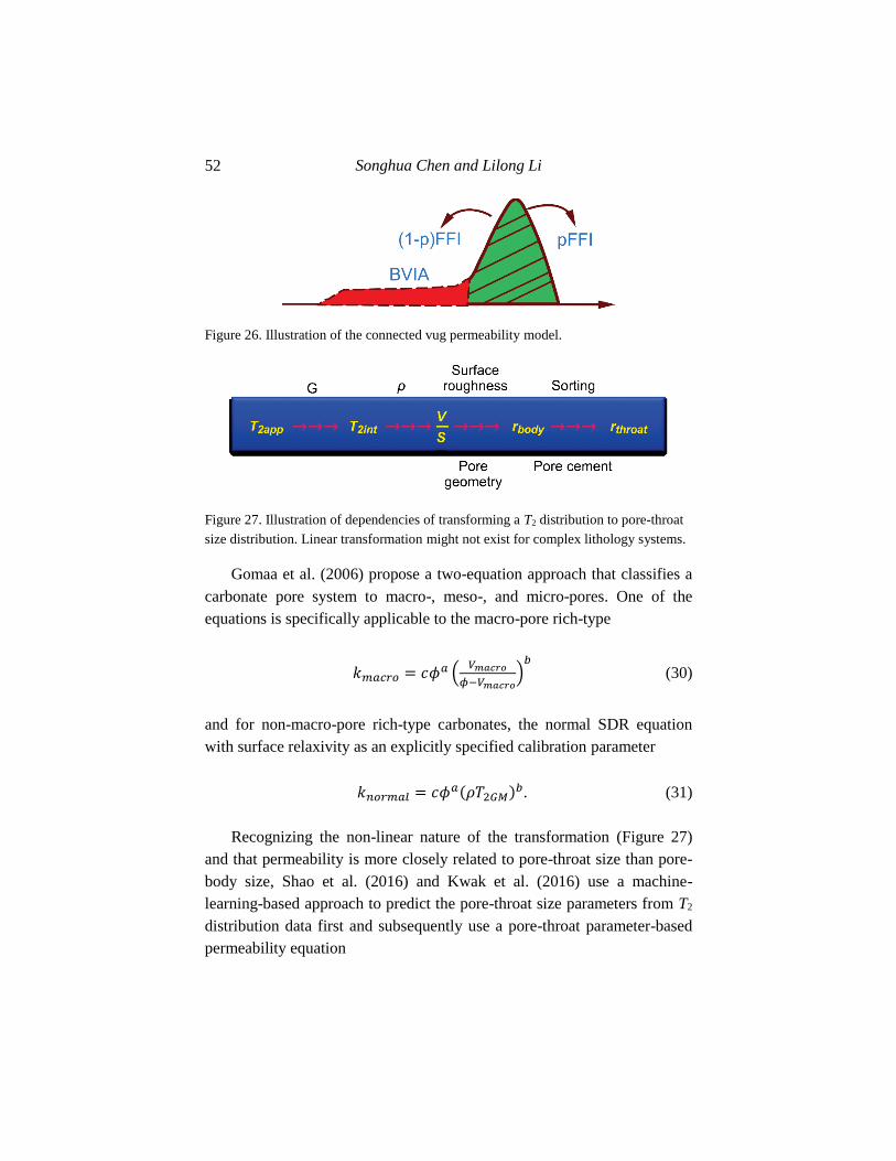
Songhua Chen and Lilong Li 52
Figure 26. Illustration of the connected vug permeability model.
Figure 27. Illustration of dependencies of transforming a T2 distribution to pore-throat
size distribution. Linear transformation might not exist for complex lithology systems.
Gomaa et al. (2006) propose a two-equation approach that classifies a
carbonate pore system to macro-, meso-, and micro-pores. One of the
equations is specifically applicable to the macro-pore rich-type
𝑘𝑚𝑎𝑐𝑟𝑜 = 𝑐𝜙𝑎 (𝑉𝑚𝑎𝑐𝑟𝑜
𝜙−𝑉𝑚𝑎𝑐𝑟𝑜)𝑏 (30)
and for non-macro-pore rich-type carbonates, the normal SDR equation
with surface relaxivity as an explicitly specified calibration parameter
𝑘𝑛𝑜𝑟𝑚𝑎𝑙 = 𝑐𝜙𝑎(𝜌𝑇2𝐺𝑀)𝑏. (31)
Recognizing the non-linear nature of the transformation (Figure 27)
and that permeability is more closely related to pore-throat size than pore-
body size, Shao et al. (2016) and Kwak et al. (2016) use a machine-
learning-based approach to predict the pore-throat size parameters from T2
distribution data first and subsequently use a pore-throat parameter-based
permeability equation

Wireline, LWD, and Surface NMR Instruments and Applications … 53
Figure 28. Crossplots of measured permeability vs. the calculated permeability using
Eq. (32) for several Middle East carbonate wells. Upper plot: the predicted
permeability using the measured MICP data-derived pore-throat size parameters. This
plot shows that the permeability is well correlated to these pore-throat size parameters;
subsequently, the optimal pore-throat-based permeability equation [Eq. (32)] is
derived. Lower plot: the measured NMR T2 distribution data are used to predict the
pore-throat size parameters using a machine-learning method. Then, the predicted
pore-throat size parameters are used in Eq. (32) to obtain the predicted permeability.

Songhua Chen and Lilong Li 54
𝑘 = 10−1.35(𝑟𝑡,𝑚𝑎𝑥)0.83
(𝑟𝑡,𝑔𝑚)0.99
𝜙1.75 (32)
to estimate permeability of Middle East carbonates. Figure 28 shows the
crossplots of measured permeability vs. the calculated permeability using
Eq. (32). The upper plot of Figure 28 shows the measured MICP data-
derived pore-throat size parameters. The plot shows that permeability is
well correlated to these pore-throat size parameters. The lower plot of
Figure 28 shows the measured NMR T2 distribution data to predict the
pore-throat size parameters using a machine-learning method. For
carbonate permeability estimations, the model performance is considered
quite good.
Because few other logging techniques can provide permeability or
permeability variation in situ, continued efforts from industry and
academia to improve permeability interpretation models are ongoing for
complex lithology wells, such as carbonates and unconventional reservoirs.
NMR FLUID CHARACTERIZATION
The volume, type, constituents, and producibility of hydrocarbon fluids
in rocks are of the ultimate interest to reservoir engineers. NMR logging
can address some of these fluid characterization issues, but others have
limitations. As discussed in previous sections, the sensitive volumes of
NMR logging are shallow and in the mud-filtrate flushed zone; therefore,
multiphase saturation determined from NMR logging is flushed-zone
saturation, which is not the same as virgin-zone saturation. This limitation,
however, does not render NMR logging useless for fluid characterization
because NMR logging can be used to detect the presence of oil, water,
and/or gas, as well as the viscosity, GOR, and other important petroleum
reservoir fluid properties.

Wireline, LWD, and Surface NMR Instruments and Applications … 55
Bulk Fluid NMR Responses
Bulk fluid (i.e., without considering surface influence on fluid
relaxation time) NMR response can be described by the mechanism of
intra-molecular, inter-molecular, and spin rotation interactions:
1
𝑇1,2𝑏=
1
𝑇1,2𝑏, 𝑖𝑛𝑡𝑟𝑎
+1
𝑇1,2𝑏𝑖𝑛𝑡𝑒𝑟+
1
𝑇1,2𝑏𝑠𝑟. (33)
Liquid hydrocarbons are dominated by the first two terms and for
simple molecules can be expressed by
1
𝑇1𝑏=
1
𝑇2𝑏= 𝐾
𝑘𝑇, (34)
where K differs by molecules, and the diffusivity of liquids also have a
similar dependency
𝐷 =𝑘𝑇
8𝜋𝑟3 (35)
for simplified molecule models. Viscosity and temperature dependencies
are interesting characteristics of fluid-typing applications. The spin rotation
mechanism dominates smaller molecules, particularly gas:
𝐷 =𝑘𝑇
6𝜋𝑟 (36)
1
𝑇1𝑏=
1
𝑇2𝑏= 𝐾′
𝑘𝑇 (37)
Note that the temperature and viscosity dependencies of the spin
rotation are the opposite of the inter- and intra-molecular interactions.

Songhua Chen and Lilong Li 56
Experimental data of more than 500 dead oil samples collected from
different fields worldwide (Chen et al, 2004) indicates that even though
crude petroleum oils vary by their molecular compositions, the geometric
mean T2 of all crude oils are quite close to the theoretical dependency of
temperature and viscosity (Figure 29)
𝑇2𝐺𝑀 = 4.97𝑇, (38)
except for highly viscous oils.
Oils with extremely high viscosity exhibit a broad distribution of T2;
the fastest-decay components of the T2 distribution might not be sensed by
NMR logging tools because of the limitation of minimal TE. Therefore, the
apparent T2 appears higher, which requires correction for viscosity
estimation. Often, an empirical, field-specific correlation is used, which
accounts for the apparent T2GM, TE, and temperature, such as that reported
by Sandor et al. (2016)
휂 =1.31𝑇𝐾
𝑇2𝐺𝑀,𝑎𝑝𝑝−1.14𝑇𝐸−0.57 (39)
for Middle East heavy oil fields.
The HI of dead oil can be calculated using (Gaymard & Poupon, 1968)
𝐻𝐼𝑜𝑖𝑙 = 9𝜌𝑜𝑖𝑙[0.15 + 0.2(0.9 − 𝜌𝑜𝑖𝑙)2], (40)
and the HI of hydrocarbon gas is (Hirasaki et al., 2003)
𝐻𝐼𝑔𝑎𝑠 =𝜌𝑔𝑎𝑠,𝑚𝑜𝑙
0.111(𝑅 (12.011 + 1.008𝑅)⁄ ), (41)
where R is the hydrogen-to-carbon ratio and ρgas,mol is the molar density of
the hydrocarbon gas. Because HIgas is significantly lower than HIoil or
HIwater even at reservoir pressure, gas is readily identified by NMR logging

Wireline, LWD, and Surface NMR Instruments and Applications … 57
with the obvious deficit in porosity, compared to other porosity logging
methods.
While laboratory measurements of oil samples are usually conducted
on dead oil samples (i.e., any gaseous components in petroleum crude oil
has been evaporated when pressure is lowered from reservoir pressure to
ambient), NMR logging is an in-situ measurement; thus, it responds to live
oil (i.e., gaseous components in the crude oil are retained). Viscosity
correlation between live oil and dead oil samples depends on whether the
live oil is in an undersaturated or saturated state. Bergman & Sutton (2007)
correlations on both saturated and undersaturated live oils are useful.
Figure 29. T2 and viscosity correlation derived from more than 500 crude oil samples
collected from petroleum-producing fields in different areas of the world (Chen
et al., 2004).

Songhua Chen and Lilong Li 58
Lo et al. (2000) derived correlations of T1,η/TK and GOR if the GOR of
a live oil is known. In their model, the measured T1 of live oil can be
expressed in terms of the linear η/TK dependence multiplied by a factor that
is a function of GOR:
𝑇1(in sec) =0.009558
𝑇𝐾𝜂
𝑓(𝐺𝑂𝑅) (42)
The HI of live oil can also be estimated based on GOR, gas and oil
densities, and viscosity.
We have discussed the NMR bulk oil responses at length because T1,
T2, and diffusivity contrasts between different fluids are the foundation for
NMR-based fluid typing, and the HI of gas and oil are important to the
accuracy of porosity estimation. In addition, HIgas is of particular
importance for discriminating gas reservoirs from liquid-filled reservoirs.
Simple Fluid Typing
Free Gas Detection
NMR-based in-situ fluid typing is generally based on T1, T2, and
diffusivity responses of hydrocarbon and water fluids or a combination of
these parameters. For NMR logging instruments that generate a significant
magnetic field gradient in the sensitive volume, comparison of T1 and T2app
contrast is an effective method of identifying gas-bearing formations
because of the order of magnitude diffusivity contrast between the
hydrocarbon gas and liquid phase.
Figure 30 shows an example comparison of T1 and T2app logs to
identify the existence of free gas in a formation. Figure 30 shows two plots
from two different shale gas plays—the gas-producing Eagle Ford shale
(left) and the Haynesville shale (right). In each plot, T1 and T2app are shown
in two tracks. Intergranular water and organic matter pore signals are
expected to have short relaxation times. However, free gas, if present, has a
long T1 and T2int, but the T2app can be significantly reduced resulting from

Wireline, LWD, and Surface NMR Instruments and Applications … 59
decay induced by diffusion in the gradient field because the free gas
diffusivity is usually an order of magnetic higher than that of the liquid-
phase fluids at the reservoir temperature. In the example shown, the
logging tool generates approximately 17 G/cm gradient strength in the
sensitive volume. With a TE of 0.9 ms, a substantial contrast between gas
T2app and T1 is expected. The long T1 relaxation time is shaded in both
tracks. The shaded T1 region for the Eagle Ford well shows a weak signal,
indicating minimal free gas. In contrast, a clear signal is observed in the
shaded T1 region of the Haynesville well, indicating free gas exists at
several depths. Neither example shows a significant signal in the long T2app
region, which further confirms the long T1 signal observed in the
Haynesville well indeed indicates free gas.
Figure 30. T1 and T2app log comparison for detecting the presence or absence of free gas
in a formation. Shown are two examples from the gas-producing Eagle Ford shale
(left) and Haynesville shale (right). Weak signal is observed in the shaded T1 region of
the Eagle Ford well, indicating minimal free gas. In contrast, a strong signal is
observed in the shaded T1 region of the Haynesville well, indicating free gas exists at
several depths. Neither example shows a significant signal in the long T2app region,
which further confirms the gas signal.
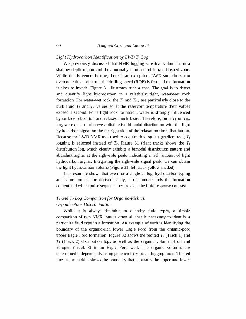
Songhua Chen and Lilong Li 60
Light Hydrocarbon Identification by LWD T1 Log
We previously discussed that NMR logging sensitive volume is in a
shallow-depth region and thus normally is in a mud-filtrate flushed zone.
While this is generally true, there is an exception. LWD sometimes can
overcome this problem if the drilling speed (ROP) is fast and the formation
is slow to invade. Figure 31 illustrates such a case. The goal is to detect
and quantify light hydrocarbon in a relatively tight, water-wet rock
formation. For water-wet rock, the T1 and T2int are particularly close to the
bulk fluid T1 and T2 values so at the reservoir temperature their values
exceed 1 second. For a tight rock formation, water is strongly influenced
by surface relaxation and relaxes much faster. Therefore, on a T1 or T2int
log, we expect to observe a distinctive bimodal distribution with the light
hydrocarbon signal on the far-right side of the relaxation time distribution.
Because the LWD NMR tool used to acquire this log is a gradient tool, T1
logging is selected instead of T2. Figure 31 (right track) shows the T1
distribution log, which clearly exhibits a bimodal distribution pattern and
abundant signal at the right-side peak, indicating a rich amount of light
hydrocarbon signal. Integrating the right-side signal peak, we can obtain
the light hydrocarbon volume (Figure 31, left track yellow shaded).
This example shows that even for a single T1 log, hydrocarbon typing
and saturation can be derived easily, if one understands the formation
content and which pulse sequence best reveals the fluid response contrast.
T1 and T2 Log Comparison for Organic-Rich vs.
Organic-Poor Discrimination
While it is always desirable to quantify fluid types, a simple
comparison of two NMR logs is often all that is necessary to identify a
particular fluid type in a formation. An example of such is identifying the
boundary of the organic-rich lower Eagle Ford from the organic-poor
upper Eagle Ford formation. Figure 32 shows the plotted T2 (Track 1) and
T1 (Track 2) distribution logs as well as the organic volume of oil and
kerogen (Track 3) in an Eagle Ford well. The organic volumes are
determined independently using geochemistry-based logging tools. The red
line in the middle shows the boundary that separates the upper and lower

Wireline, LWD, and Surface NMR Instruments and Applications … 61
Eagle Ford formation. It is observed that the T1 and T2 distributions of the
organic-poor upper Eagle Ford exhibits much more irregular patterns from
depth to depth. The wider distributions indicate it is more affected by
surface relaxation and pore sizes, which indicates an insignificant influence
by organic matter. In contrast, the T1 and T2 distributions of the organic-
rich lower Eagle Ford depths show much more regular, narrow distribution
patterns, indicating the signal is not much affected by pore sizes but rather
reflects the relatively consistent organic content influence in the relaxation
time response.
Figure 31. Example of using LWD T1 logging to identify and quantify light oil volume
in a tight rock formation.

Songhua Chen and Lilong Li 62
Such pattern is repeatable from well to well in the Eagle Ford
formation. While distribution patterns require experienced log analysts to
identify, the next example shows thatone can simply compare the T1GM,
T2GM, or T1GM/T2GM (Figure 33) with logging data acquired from a different
Eagle Ford well. By examining a sudden shift of T1GM, T2GM, or T1GM/T2GM,
one can readily identify the boundary between the organic-poor upper
Eagle Ford and the organic-rich lower Eagle Ford.
It is important to mention that the NMR T1 and T2 response to organic-
rich pore fluids depends on the resonance frequency, minimal TE (TEmin)
used to acquire logs, and possibly the maturity of organic matter in the
reservoir. Therefore, field and tool-based interpretation models are
essential. A model developed in one shale play with one logging
instrument operating in certain frequency range might not be applicable to
a different formation and different logging tool that operates at different
resonance frequency and TEmin.
Figure 32. Upper and lower Eagle Ford T1 and T2 distribution patterns indicate the
difference between the organic-rich lower Eagle Ford and the organic-poor upper
Eagle Ford.

Wireline, LWD, and Surface NMR Instruments and Applications … 63
Figure 33. By examining the T1GM, T2GM, or T1GM/T2GM shift, one can readily identify the
boundary between the organic-rich lower Eagle Ford and the organic-poor upper
Eagle Ford.
Multi-Dimensional Fluid Typing
In the previous section, we presented examples that illustrate that
simple 1D NMR logs can satisfactorily obtain fluid-typing information.
For more complicated cases, 1D logging might be insufficient to non-
ambiguously identify fluid types, particularly if significant overlapping and
blurring of different fluids in NMR responses occur. In such case, 2D and
3D logs might provide additional contrasts to reduce uncertainties.
2D T1 − T2app Map
Simple application of a T1 − T2app map can identify gas in a reservoir.
This is similar to the separate 1D T1 and T2app logs (Figure 30) but in the

Songhua Chen and Lilong Li 64
form of cross plotting T1 and T2app (Figure 34). The upper plot is acquired
at a gas-bearing depth in the Haynesville formation and shows a free-gas
signal (circled) that corresponds to long T1 but short T2app. The bottom plot
is acquired at a gas-producing depth in an Eagle Ford well. Although
production data prove it is a gas-bearing formation, no free-gas signal is
detected on the NMR 2D map, such as that observed in the Haynesville
reservoir. Therefore, the produced gas is likely from the organic pores and
in adsorption state.
Figure 34. Free-gas detection from T1 − T2app map. The upper plot is from a gas-
producing depth in a Haynesville well, and the lower plot is from a gas-producing
depth in an Eagle Ford well. The former shows the presence of free gas (circled) in
intergranular space, as evidenced by the large T1/T2app because the high diffusivity of
free gas causes faster T2app decay in a magnetic field gradient. The lower plot shows
zero free gas. Thus, the produced gas is mostly from the nanopores in organic matter.

Wireline, LWD, and Surface NMR Instruments and Applications … 65
2D D − T2int Map
Figure 35 shows an example of a 2D D − T2int map for oil and water
discernment. The NMR log is acquired in a carbonate reef formation. The
well is drilled with WBM. The two plots in Figure 35 correspond to two
different depths.
To help interpret the data, three lines are displayed on the map. The red
dashed line represents free gas at the reservoir temperature, the light-blue
dashed line represents water, and the green slanted line represents the oil
line, where the location of the oil line is determined by the oil viscosity.
In this case, the strong, bright signal at the rightmost side of the 2D
map display represents the water signal in large pores, which is likely from
the invaded WBM filtrate. The green oval closure on the left side
highlights the oil signal located on the oil line, which indicates the
presence of oil in the formation rock at this depth. However, the oil signal
is absent near the other depth (right-side plot), indicating it is not oil-
bearing. Although these two signals appear separable from T2 distribution
alone, showing it in a 2D D − T2int map helps increase confidence in the oil
signal interpretation because of the additional contrast in diffusivity.
Figure 35. 2D D − T2int map for oil and water discrimination. The green circled region
represents oil in the formation, and the white circled region represents water in the
large pores of this carbonate reef formation. The water likely originates from the
invaded WBM filtrate. The left plot indicates oil is present at this depth of the
formation while oil is absent from the depth corresponding to the right plot.

Songhua Chen and Lilong Li 66
2D D − T1 Map
A D − T2int map is a useful tool for fluid typing. However, T2 is
sensitive to secondary effects, such as the geometric restriction of diffusion
in confined pores, as well as the internal field gradient that originates from
the variation of magnetic minerals in the rock matrices. Because these
effects are not always quantifiable and thus might not have been accounted
for in the NMR data inversion, the results can have some shift of the
relative positions of oil and water, causing difficulties during fluid-typing
interpretation. Figure 36 shows a tight oil well example. The left plot
shows a D − T2int map, where the oil and water signals are slightly
Figure 36. Illustration of the D – T1 map value. Because T2 might be subject to
unknown internal gradient and restricted diffusion, which could distort the D − T2int
map (left), an additional D – T1 map (right) sometimes helps simplify interpretation
because T1 is not subject to the internal (and external) field gradient. In this case, the
oil and water are much more clearly separated on the D – T1 map.

Wireline, LWD, and Surface NMR Instruments and Applications … 67
distorted, causing difficulty in interpretation. The right plot shows the D –
T1 map of the same depth. In the absence of the internal field gradient
effect, the water and oil signals are much more clearly separated.
Figure 37. Illustration of a 3D map used to reduce the uncertainty of identifying heavy
oil in a reservoir formation. Because heavy oil generally has a T1/T2int ratio larger than
unity, observing a shift of signal position between D − T1 and D − T2int maps helps
reduce the ambiguity between heavy oil and bound water. The high T1/T2int (>3) of the
heavy oil signal is also confirmed by the T1 − T2int map.
3D Map Applications
Because of the finite gradient strength, which is determined by the
logging tool design, the sensitivity of diffusivity is limited, particularly if

Songhua Chen and Lilong Li 68
the relaxation time is fast. This causes difficulty in discerning heavy oil
from water on a single D − T2int or D – T1 plot. However, as discussed in
the NMR Fluid Characterization section, heavy oil corresponds to a higher
T1/T2int than unity; thus, a 3D display can be helpful. Figure 37 shows a
shift between T1 and T2int on the D − T2int and D – T1 plots from a heavy oil
well. The plot of T1 − T2int (bottom) further confirms that the signal in
question has T1/T2int centered around 3, which is higher than that expected
for bound water. For comparison, Figure 38 shows a similar 3D map from
a nearby water-bearing depth in the same well, where the bound water
shows no signal shift between T1 and T2int on the D − T2int and D – T1 plots
(upper two plots), and T1 − T2int plots (bottom) show the T1/T2int is centered
quite close to the unity line.
Figure 38. As a comparison to the heavy oil-bearing formation, a water-bearing, clay,
and silt-rich formation depth is shown. No shift of signal position between D − T1 and
D − T2int maps is observed, and T1/T2int is approximately 1 on the T1 − T2int map, which
is also much smaller than that of the heavy oil signature.

Wireline, LWD, and Surface NMR Instruments and Applications … 69
Figure 39. D − T2int and D − T1 maps of a complex mineralogy well containing a
heterogeneous amount of iron-rich minerals. Analyzing these 2D maps alone, one
might conclude that a represents oil and b represents water. Figure 40 shows that
further analysis provides a different interpretation.
Figure 40. D − T2 submaps of the same well shown in Figure 39. The three submaps
correspond to R (≡ T1/T2int) of 1, 3, and 5, respectively. Clearly, the majority of signals
are shown only on R = 1 and R = 5 but not R = 3 submaps. The reservoir formation
contains iron-rich minerals that could induce high internal gradient, which affects the
wetting-phase fluid (water) more significantly than the non-wetting-phase fluid.
Therefore, the signal corresponding to R = 1 is interpreted as oil, and the signal
corresponding to R = 5 is water.
The next example emphasizes the importance of examining the maps
from various angles. Figure 39 shows the D − T2int and D – T1 maps of a
complex minerology well, where an unspecified, varying amount of
magnetic minerals are present from depth to depth. From these two maps,
one might conclude signal a likely indicates oil, and signal b likely
indicates water, even though they are slightly off their ideal lines.
Songhua Chen and Lilong Li 70
After further plotting the D − T2int map in sets of three submaps
corresponding to R = T1/T2int of 1, 3, and 5, respectively (Figure 40), we
determined that a portion of signal a in Figure 37 corresponds to R = 1,
while the entire signal b and part of signal a in Figure 39 corresponds to R
= 5, and negligible signal corresponds to R = 3. This fact, when interpreted
with iron-rich minerals at the depth, leads to the conclusion that the signal
corresponding to R = 5 is water, which as a wetting-phase fluid is strongly
affected by the internal field gradient caused by the iron-rich minerals.
Thereby, the apparent R increases. However, oil as a non-wetting-phase
fluid is much less affected by the internal field gradient.
This section discussed several examples of the usefulness of 2D and
3D maps for fluid typing. As the formations of petroleum-producing
reservoirs become increasingly complicated, particularly with many
unconventional reservoirs, tight rock formations, and carbonate formations
becoming increasingly important for oil production, it is expected that the
use of 2D and 3D maps for formation evaluation interpretation will
increase in the future.
ACKNOWLEDGMENTS
The authors thank their colleagues, Wei Shao, Ron Balliet, Arcady
Reiderman, and many others for providing several figures and for the
stimulating discussions that contributed to this work. We also thank
Halliburton management for their support of publishing this chapter.
REFERENCES
Ahmed, U., Crary, S. F. & Coates, G. R. (1991). Permeability Estimation:
The Various Sources and Their Interrelationships. J Pet Technol, 43
(05), 578-587.
Akkurt, R., Fransson, C. M., Witkowsky, J. M., Langley, W. M., Sun, B. &
McCarty, A. (2004). Fluid Sampling and Interpretation with the

Wireline, LWD, and Surface NMR Instruments and Applications … 71
Downhole NMR Fluid Analyzer. Paper presented at the SPE Annual
Technical Conference and Exhibition, Houston, Texas, September 26-
29. SPE-90971-MS.
Beard, D. (2007). Frequency dithering to avoid excitation pulse ringing.
Patent No. US7301337.
Bergman, D. F. & Sutton, R. P. (2007). An Update to Viscosity
Correlations for Gas-Saturated Crude Oils. Paper presented at the SPE
Annual Technical Conference and Exhibition, Anaheim, California,
November 11-14. SPE-110195-MS.
Chang, D., Vinegar, H. J., Morriss, C. E. & Straley, C. (1997). Effective
Porosity, Producible Fluid, and Permeability in Carbonates From NMR
Logging. The Log Analyst, 38 (2), 60-72.
Chen, S. (2010). Echo-decay-acceleration data acquisition method for gas
identification using a low-field gradient. Patent No. US7808238.
Chen, S. & Edwards, C. M. (2002). Objective oriented methods for NMR
log acquisitions for estimating earth formation and fluid properties.
Patent No. US6972564.
Chen, S., Jacobi, D., Kwak, H., Altunbay, M. & Kloos, J. (2008). Pore-
Connectivity Based Permeability Model For Complex Carbonate
Formations. Paper presented at the SPWLA 49th Annual Logging
Symposium, Austin, Texas, May 25-28. SPWLA-2008-E.
Chen, S., Shao, W. & Balliet, R. (2016). New, Robust Multidimensional
NMR Inversion Methods for Improving Fluid Typing and Rock
Characterization. Paper presented at the SPWLA 57th Annual
Logging Symposium, Reykjavik, Iceland, June 25-29. SPWLA-2016-
GG.
Chen, S., Zhang, G., Kwak, H., Edwards, C. M., Ren, J. & Chen, J. (2004).
Laboratory Investigation of NMR Crude Oils and Mud Filtrates
Properties in Ambient and Reservoir Conditions. Paper presented at
the SPE Annual Technical Conference and Exhibition, Houston,
Texas, September 26-29. SPE-90553-MS.
Edwards, J. C. (2011). A Review of Applications of NMR Spectroscopy in
Petroleum Chemistry. In R. A. Kishore Nadkarni (Ed.), Spectroscopic

Songhua Chen and Lilong Li 72
Analysis of Petroleum Products and Lubricants, (pp. 423-473). West
Conshohocken, Pennsylvania: ASTM International.
Flaum, C. (2000). Nuclear magnetic resonance well logging to determine
gas-filled porosity and oil-filled porosity of earth formations without a
constant static magnetic field gradient. Patent No. US6097184.
Freed, D., Hürlimann, M. D. & Scheven, U. (2001). Nuclear magnetic
resonance logging based on steady-state free precession. Patent No.
US6580272.
Gaymard, R. & Poupon, A. (1968). Response Of Neutron And Formation
Density Logs In Hydrocarbon Bearing Formations. The Log Analyst, 9
(05), 3-20.
Goelman, G. & Prammer, M. G. (1995). The CPMG Pulse Sequence in
Strong Magnetic Field Gradients with Applications to Oil-Well
Logging. J. Magn. Reson., Ser A, 113 (1), 11-18.
Gomaa, N. M., Azer, S. R., Ouzzane, D. E., Saif, O., Okuyiga, M. O.,
Allen, D. F., Rose, D., Ramamoorthy, R. & Bize, E. (2006). Case
Study of Permeability, Vug Quantification, and Rock Typing in a
Complex Carbonate. Paper presented at the SPE Annual Technical
Conference and Exhibition, San Antonio, Texas, September 24-27.
SPE-102888-MS.
Hidajat, I., Mohanty, K. K., Flaum, M. & Hirasaki, G. (2004). Study of
Vuggy Carbonates Using NMR and X-Ray CT Scanning. SPE Res
Eval & Eng, 7 (05), 365-377.
Hirasaki, G. J., Lo, S. W. & Zhang, Y. (2003). NMR properties of
petroleum reservoir fluids. Magnetic Resonance Imaging, 21 (3-4),
269-277.
Hürlimann, M. D. (2001). Diffusion and Relaxation Effects in General
Stray Field NMR Experiments. J. Magn. Reson., 148 (2), 367-378.
Hürlimann, M. D. & Griffin, D. D. (2000). Spin Dynamics of Carr-Purcell-
Meiboom-Gill-like Sequences in Grossly Inhomogeneous B0 and B1
Fields and Application to NMR Well Logging. J. Magn. Reson., 143
(1), 120-135.
Hürlimann, M. D., Venkataramanan, L., Flaum, C., Speier, P., Karmonik,
C., Freedman, R. & Heaton, N. (2002). Diffusion-Editing: New Nmr

Wireline, LWD, and Surface NMR Instruments and Applications … 73
Measurement Of Saturation And Pore Geometry. Paper presented at
the SPWLA 43rd Annual Logging Symposium, Oiso, Japan, June 2-5.
SPWLA-2002-FFF.
Jachmann, R. C., Li, L. & Reiderman, A. (2017). Nuclear magnetic
resonance apparatus, systems, and methods. Patent No. US9784881.
Jachmann, R., Yang, J. & Chen, S. (2013). New Data Processing with new
Generation Magnetic Resonance While Drilling Tool. Paper presented
at the SPWLA 54th Annual Logging Symposium, New Orleans,
Louisiana, June 22-26. SPWLA-2013-UU.
Jackson, J. A. (2001). The History of NMR Well Logging. Concepts
Magn. Reson., 13 (6), 340-411.
Jackson, J. A. & Cooper, R. K. (1982). Magnetic resonance apparatus.
Patent No. US4350955.
Kenyon, W. E., Day, P. I., Straley, C. & Willemsen, J. F. (1986). Compact
and Consistent Representation of Rock NMR Data for Permeability
Estimation. Paper presented at the SPE Annual Technical Conference
and Exhibition, New Orleans, Louisiana, October 5-8.
Kwak, H., Hursan, G., Shao, W., Chen, S., Balliet, R., Eid, M. &
Guergueb, N. (2016). Predicting Carbonate Rock Properties Using
NMR Data and Generalized Interpolation-Based Techniques.
Petrophysics, 57 (4), 351-368.
Lo, S. W., Hirasaki, G. J., House, W. V. & Kobayashi, R. (2000). Mixing
Rules and Correlations of NMR Relaxation Time With Viscosity,
Diffusivity, and Gas/Oil Ratio of Methane/Hydrocarbon Mixtures. SPE
J., 7 (01), 24-34.
MacInnis, J. P., Macune, D. T., Morriss, C. E., Oldigs, R. W., Smaardyk, J.
E. & Steiner, Jr. J. M. (1995). Borehole measurement of NMR
characteristics of earth formation. Patent No. US5432446.
Nordin, M. & Knight, R. (2016). The effect of surface roughness on
Nuclear Magnetic Resonance relaxation. diffusion-fundamentals.org,
26 (3), 1-11.
Prammer, M. G., Bouton, J. C., Masak, P. & Drack, E. D. (2007).
Magnetic resonance fluid analysis apparatus and method. Patent No.
US7164267.

Songhua Chen and Lilong Li 74
Reiderman, A. & Chen, S. (2015). Downhole Nuclear Magnetic Resonance
(NMR) Tool with Transversal-Dipole Antenna Configuration. Patent
No. US20150061664.
Reiderman, A. & Chen, S. (2016). Azimuthally-selective downhole nuclear
magnetic resonance (NMR) tool. Patent No. US 9377557.
Sandor, M., Cheng, Y. & Chen, S. (2016). Improved Correlations for
Heavy-Oil Viscosity Prediction with NMR. J. Petrol. Sci. Eng., 147,
416-426.
Sezginer, A. & Straley, C. (1995). Nuclear magnetic resonance pulse
sequences for determining bound fluid volume. Patent No. US5389877.
Shao, W., Chen, S., Cheng, Y., Eid, M. & Hursan, G. (2016). Improved
RBF-Based NMR Pore-Throat Size, Pore Typing, and Permeability
Models for Middle East Carbonates. Paper presented at the SPE
Annual Technical Conference and Exhibition, Dubai, UAE, September
26-28. SPE-181448-MS.
Toumelin, E., Torres-Verdin, C. & Chen, S. (2003). Modeling of Multiple
Echo-Time NMR Measurements for Complex Pore Geometries and
Multiphase Saturations. SPE Res Eval & Eng, 6 (04), 234-243.


![Deep Borehole Field Test Laboratory and Borehole Testing ... · The characterization borehole (CB) is the smaller-diameter borehole (i.e., 21.6 cm [8.5”] diameter at total depth),](https://static.fdocuments.net/doc/165x107/5ebe68817151f10bcd35645a/deep-borehole-field-test-laboratory-and-borehole-testing-the-characterization.jpg)